

Page 1

Guide to Using
@RISK for Six
Sigma
Version 5.5
May, 2009
Palisade Corporation
798 Cascadilla St.
Ithaca, NY USA 14850
(607) 277-8000
(607) 277-8001 (fax)
http://www.palisade.com (website)
sales@palisade.com (e-mail)
Page 2

Copyright Notice
Copyright © 2009, Palisade Corporation.
Trademark Acknowledgments
Microsoft, Excel and Windows are registered trademarks of Microsoft, Inc.
IBM is a registered trademark of International Business Machines, Inc.
Palisade, TopRank, BestFit and RISKview are registered trademarks of Palisade
Corporation.
RISK is a trademark of Parker Brothers, Division of Tonka Corporation and is used under
license.
Page 3

Welcome
Welcome to @RISK, the world’s most powerful risk analysis tool!
@RISK has long been used to analyze risk and uncertainty in any
industry. With applications in finance, oil and gas, insurance,
manufacturing, healthcare, pharmaceuticals, science and other fields,
@RISK is as flexible as Excel itself. Every day tens of thousands of
professionals use @RISK to estimate costs, analyze NPV and IRR,
study real options, determine pricing, explore for oil and resources,
and much more.
A key application of @RISK is Six Sigma and quality analysis.
Whether it’s in DMAIC, Design for Six Sigma (DFSS), Lean projects,
Design of Experiments (DOE), or other areas, uncertainty and variable
lies at the core of any Six Sigma analysis. @RISK uses Monte Carlo
simulation to identify, measure, and root out the causes of variability
in your production and service processes. A full suite of capability
metrics gives you the calculations you need to step through any Six
Sigma method quickly and accurately. Charts and tables clearly show
Six Sigma statistics, making it easy and effective to illustrate this
powerful technique to management. The Industrial edition of @RISK
adds RISKOptimizer to your Six Sigma analyses for optimization of
project selection, resource allocation, and more.
Industries ranging from engine manufacturing to precious metals to
airlines and consumer goods are using @RISK every day to improve
their processes, enhance the quality of their products and services,
and save millions. This guide will walk you through the @RISK Six
Sigma functions, statistics, charts and reports to show you how
@RISK can be put to work at any stage of a Six Sigma project.
Example case studies round out the guide, giving you pre-built
models you can adapt to your own analyses.
The standard features of @RISK, such as entering distribution
functions, fitting distributions to data, running simulations and
performing sensitivity analyses, are also applicable to Six Sigma
models. When using @RISK for Six Sigma modeling you should also
familiarize yourself with these features by reviewing the @RISK for
Excel Users Guide and on-line training materials.
Page 4

Page 5

Table of Contents
Chapter 1: Overview of @RISK and Six Sigma Methodologies 1
Introduction.........................................................................................3
Six Sigma Methodologies..................................................................7
@RISK and Six Sigma........................................................................9
Chapter 2: Using @RISK for Six Sigma 13
Introduction.......................................................................................15
RiskSixSigma Property Function....................................................17
Six Sigma Statistics Functions .......................................................21
Six Sigma and the Results Summary Window ..............................35
Six Sigma Markers on Graphs.........................................................37
Case Studies 39
Example 1 – Design of Experiments: Catapult..............................41
Example 2 – Design of Experiments: Welding...............................47
Example 3 – Design of Experiments with Optimization................53
Example 4 – DFSS: Electrical Design.............................................61
Example 5 – Lean Six Sigma: Analysis of Current State – Quotation
Process...........................................................................................63
Example 6 – DMAIC: Roll Through Yield Analysis........................73
Example 7 – Vendor Selection ........................................................77
Table of Contents v
Page 6

Example 8 – Six Sigma DMAIC Failure Rate..................................81
Example 9 – Six Sigma DMAIC Failure Rate using RiskTheo......85
vi Introduction
Page 7

Chapter 1: Overview of @RISK and Six Sigma Methodologies
Introduction.........................................................................................3
What is Six Sigma?...................................................................................3
The Importance of Variation..................................................................5
Six Sigma Methodologies..................................................................7
Six Sigma / DMAIC .................................................................................7
Design for Six Sigma (DFSS).................................................................7
Lean or Lean Six Sigma...........................................................................8
@RISK and Six Sigma........................................................................9
@RISK and DMAIC.................................................................................9
@RISK and Design for Six Sigma (DFSS) .........................................10
@RISK and Lean Six Sigma..................................................................11
@RISK 5.0 Help System © Palisade Corporation, 1999
Chapter 1: Overview of @RISK and Six Sigma Methodologies 1
Page 8

2 Introduction
Page 9

Introduction
In today’s competitive business environment, quality is more
important than ever. Enter @RISK, the perfect companion for any Six
Sigma or quality professional. This powerful solution allows you to
quickly analyze the effect of variation within processes and designs.
In addition to Six Sigma and quality analysis, @RISK can be used to
analyze any situation in which there is uncertainty. Applications
include analysis of NPV, IRR, and real options, cost estimation,
portfolio analysis, oil and gas exploration, insurance reserves, pricing,
and much more. To learn more about @RISK in other applications,
and the use of @RISK in general, refer to the @RISK User’s Guide
included with your software.
What is Six Sigma?
Six Sigma is a set of practices to systematically improve processes by
reducing process variation and thereby eliminating defects. A defect
is defined as nonconformity of a product or service to its
specifications. While the particulars of the methodology were
originally formulated by Motorola in the mid-1980s, Six Sigma was
heavily inspired by six preceding decades of quality improvement
methodologies such as quality control, TQM, and Zero Defects. Like
its predecessors, Six Sigma asserts the following:
• Continuous efforts to reduce variation in process outputs is key
to business success
• Manufacturing and business processes can be measured,
analyzed, improved and controlled
• Succeeding at achieving sustained quality improvement
requires commitment from the entire organization, particularly
from top-level management
Six Sigma is driven by data, and frequently refers to “X” and “Y”
variables. X variables are simply independent input variables that
affect the dependent output variables, Y. Six Sigma focuses on
identifying and controlling variation in X variables to maximize
quality and minimize variation in Y variables.
Chapter 1: Overview of @RISK and Six Sigma Methodologies 3
Page 10
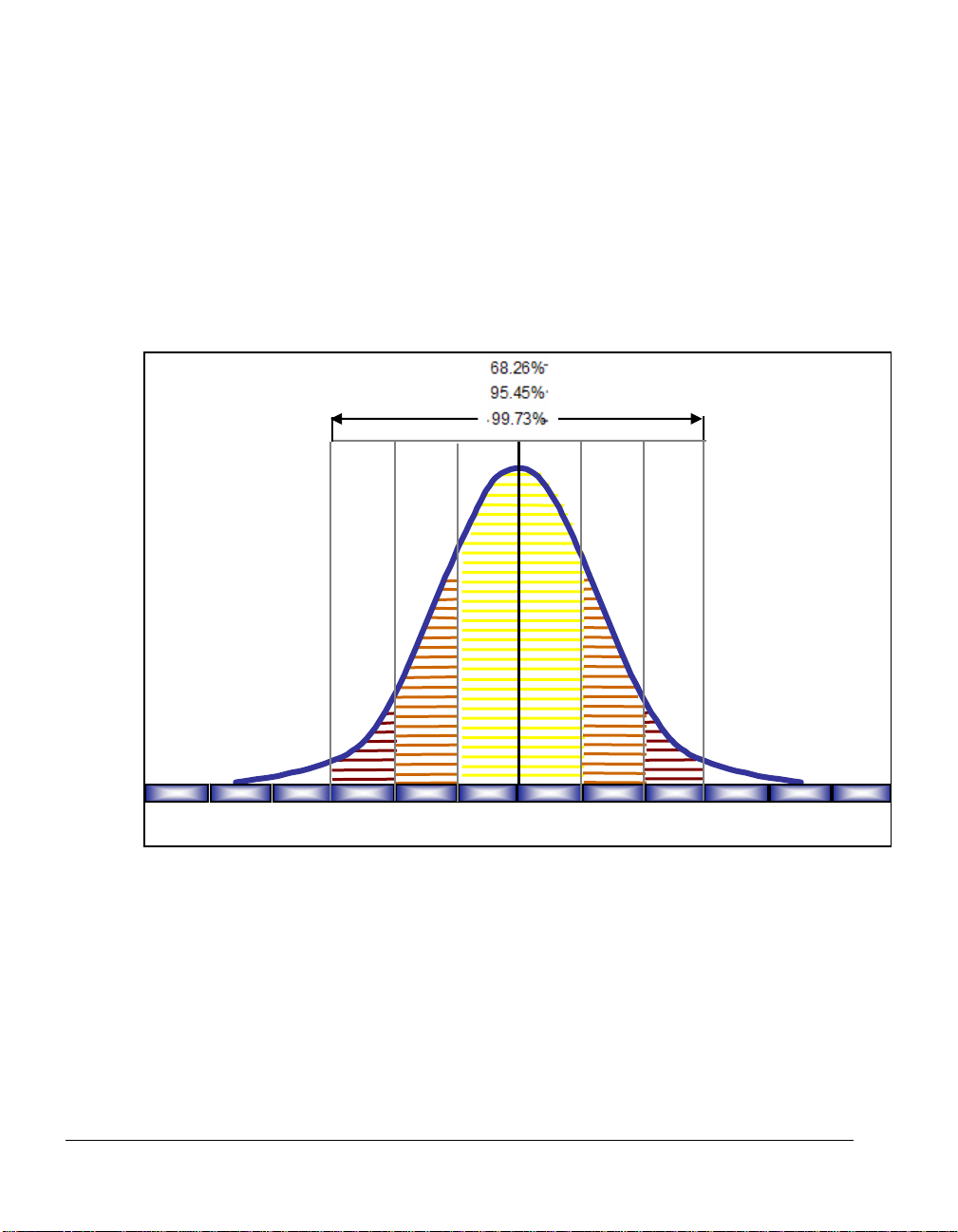
The term Six Sigma or 6σ is very descriptive. The Greek letter sigma
(σ) signifies standard deviation, an important measure of variation.
The variation of a process refers to how tightly all outcomes are
clustered around the mean. The probability of creating a defect can
be estimated and translated into a “Sigma level.” The higher the
Sigma level, the better the performance. Six Sigma refers to having
six standard deviations between the average of the process center
and the closest specification limit or service level. That translates to
fewer than 3.4 defects per one million opportunities (DPMO). The
chart below illustrates Six Sigma graphically.
-6
-3 -4 -5
-2
-1
+1
+4 +3 +2
+5
Six sigmas – or standard deviations – from the mean.
The cost savings and quality improvements that have resulted from
Six Sigma corporate implementations are significant. Motorola has
reported $17 billion in savings since implementation in the mid 1980s.
Lockheed Martin, GE, Honeywell, and many others have experienced
tremendous benefits from Six Sigma.
4 Introduction
+6
Page 11

The Importance of Variation
Too many Six Sigma practitioners rely on static models that don’t
account for inherent uncertainty and variability in their processes or
designs. In the quest to maximize quality, it’s vital to consider as
many scenarios as possible.
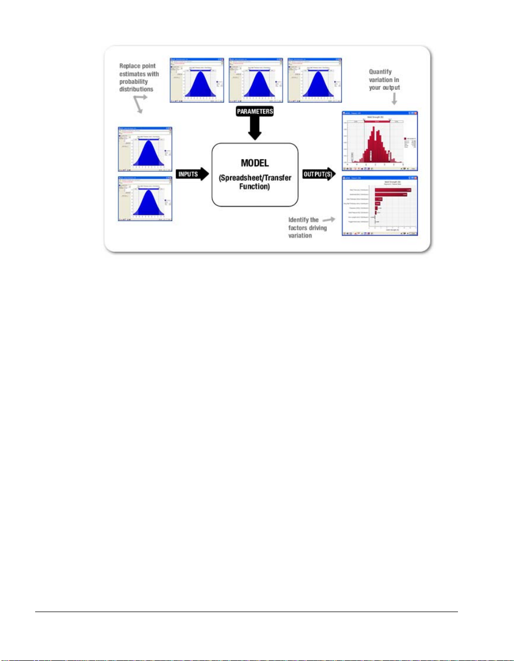
That’s where @RISK comes in. @RISK uses Monte Carlo simulation to
analyze thousands of different possible outcomes, showing you the
likelihood of each occurring. Uncertain factors are defined using over
35 probability distribution functions, which accurately describe the
possible range of values your inputs could take. What’s more, @RISK
allows you to define Upper and Lower Specification Limits and
Target values for each output, and comes complete with a wide range
of Six Sigma statistics and capability metrics on those outputs.
@RISK Industrial edition also includes RISKOptimizer, which
combine the power of Monte Carlo simulation with genetic algorithmbased optimization. This gives you the ability to tackle optimization
problems like that have inherent uncertainty, such as:
• resource allocation to minimize cost
• project selection to maximize profit
• optimize process settings to maximize yield or minimize cost
• optimize tolerance allocation to maximize quality
• optimize staffing schedules to maximize service
The figure here illustrates how @RISK helps to identify, quantify, and
hone in on variation in your processes.
Chapter 1: Overview of @RISK and Six Sigma Methodologies 5
Page 12
6 Introduction
Page 13

Six Sigma Methodologies
@RISK can be used in a variety of Six Sigma and related analyses. The
three principal areas of analysis are:
• Six Sigma / DMAIC / DOE
• Design for Six Sigma (DFSS)
• Lean or Lean Six Sigma
Six Sigma / DMAIC
When most people refer to Six Sigma, they are in fact referring to the
DMAIC methodology. The DMAIC methodology should be used
when a product or process is in existence but is not meeting customer
specification or is not performing adequately.
DMAIC focuses on evolutionary and continuous improvement in
manufacturing and services processes, and is almost universally
defined as comprising of the following five phases: Define, Measure,
Analyze, Improve and Control:
1) Define the project goals and customer (internal and external
Voice of Customer or VOC) requirements
2) Measure the process to determine current performance
3) Analyze and determine the root cause(s) of the defects
4) Improve the process by eliminating defect root causes
5) Control future process performance
Design for Six Sigma (DFSS)
DFSS is used to design or re-design a product or service from the
ground up. The expected process Sigma level for a DFSS product or
service is at least 4.5 (no more than approximately 1 defect per
thousand opportunities), but can be 6 Sigma or higher depending on
the product. Producing such a low defect level from product or
service launch means that customer expectations and needs (CriticalTo-Qualities or CTQs) must be completely understood before a design
can be completed and implemented. Successful DFSS programs can
reduce unnecessary waste at the planning stage and bring products to
market more quickly.
Chapter 1: Overview of @RISK and Six Sigma Methodologies 7
Page 14

Unlike the DMAIC methodology, the phases or steps of DFSS are not
universally recognized or defined -- almost every company or
training organization will define DFSS differently. One popular
Design for Six Sigma methodology is called DMADV, and retains the
same number of letters, number of phases, and general feel as the
DMAIC acronym. The five phases of DMADV are defined as: Define,
Measure, Analyze, Design and Verify:
1) Define the project goals and customer (internal and external
VOC) requirements
2) Measure and determine customer needs and specifications;
benchmark competitors and industry
3) Analyze the process options to meet the customer needs
4) Design (detailed) the process to meet the customer needs
5) Verify the design performance and ability to meet customer
needs
Lean or Lean Six Sigma
“Lean Six Sigma” is the combination of Lean manufacturing
(originally developed by Toyota) and Six Sigma statistical
methodologies in a synergistic tool. Lean deals with improving the
speed of a process by reducing waste and eliminating non-value
added steps. Lean focuses on a customer “pull” strategy, producing
only those products demanded with “just in time” delivery. Six
Sigma improves performance by focusing on those aspects of a
process that are critical to quality from the customer perspective and
eliminating variation in that process. Many service organizations, for
example, have already begun to blend the higher quality of Six Sigma
with the efficiency of Lean into Lean Six Sigma.
Lean utilizes “Kaizen events” -- intensive, typically week-long
improvement sessions -- to quickly identify improvement
opportunities and goes one step further than a tradition process map
in its use of value stream mapping. Six Sigma uses the formal DMAIC
methodology to bring measurable and repeatable results.
Both Lean and Six Sigma are built around the view that businesses are
composed of processes that start with customer needs and should end
with satisfied customers using your product or service.
8 Six Sigma Methodologies
Page 15

@RISK and Six Sigma
Whether it’s in DMIAC, Design of Experiments or Lean Six Sigma,
uncertainty and variability lie at the core of any Six Sigma analysis.
@RISK uses Monte Carlo simulation to identify, measure, and root out
the causes of variability in your production and service processes.
Each of the Six Sigma methodologies can benefit from @RISK
throughout the stages of analysis.
@RISK and DMAIC
@RISK is useful at each stage of the DMAIC process to account for
variation and hone in on problem areas in existing products.
1) Define. Define your process improvement goals,
incorporating customer demand and business strategy.
Value-stream mapping, cost estimation, and identification of
CTQs (Critical-To-Qualities) are all areas where @RISK can
help narrow the focus and set goals. Sensitivity analysis in
@RISK zooms in on CTQs that affect your bottom-line
profitability.
2) Measure. Measure current performance levels and their
variations. Distribution fitting and over 35 probability
distributions make defining performance variation accurate.
Statistics from @RISK simulations can provide data for
comparison against requirements in the Analyze phase.
3) Analyze. Analyze to verify relationship and cause of
defects, and attempt to ensure that all factors have been
considered. Through @RISK simulation, you can be sure all
input factors have been considered and all outcomes
presented. You can pinpoint the causes of variability and risk
with sensitivity and scenario analysis, and analyze tolerance.
Use @RISK’s Six Sigma statistics functions to calculate
capability metrics which identify gaps between
measurements and requirements. Here we see how often
products or processes fail and get a sense of reliability.
Chapter 1: Overview of @RISK and Six Sigma Methodologies 9
Page 16

4) Improve. Improve or optimize the process based upon the
analysis using techniques like Design of Experiments.
Design of Experiments includes the design of all informationgathering exercises where variation is present, whether under
the full control of the experimenter or not. Using @RISK
simulation, you can test different alternative designs and
process changes. @RISK is also used for reliability analysis
and – using RISKOptimizer - resource optimization at this
stage.
5) Control. Control to ensure that any variances are corrected
before they result in defects. In the Control stage, you can
set up pilot runs to establish process capability, transition to
production and thereafter continuously measure the process
and institute control mechanisms. @RISK automatically
calculates process capability and validates models to make
sure that quality standards and customer demands are met.
@RISK and Design for Six Sigma (DFSS)
One of @RISK’s main uses in Six Sigma is with DFSS at the planning
stage of a new project. Testing different processes on physical
manufacturing or service models or prototypes can be cost
prohibitive. @RISK allows engineers to simulate thousands of
different outcomes on models without the cost and time associated
with physical simulation. @RISK is helpful at each stage of a DFSS
implementation in the same way as the DMAIC steps. Using @RISK
for DFSS gives engineers the following benefits:
• Experiment with different designs / Design of Experiments
• Identify CTQs
• Predict process capability
• Reveal product design constraints
• Cost estimation
• Project selection – using RISKOptimizer to find the optimal
portfolio
• Statistical tolerance analysis
• Resource allocation – using RISKOptimizer to maximize
efficiency
10 @RISK and Six Sigma
Page 17

@RISK and Lean Six Sigma
@RISK is the perfect companion for the synergy of Lean
manufacturing and Six Sigma. “Quality only” Six Sigma models may
fail when applied to reducing variation in a single process step, or to
processes which do not add value to the customer. For example, an
extra inspection during the manufacturing process to catch defective
units may be recommended by a Six Sigma analysis. The waste of
processing defective units is eliminated, but at the expense of adding
inspection which is in itself waste. In a Lean Six Sigma analysis,
@RISK identifies the causes of these failures. Furthermore, @RISK can
account for uncertainty in both quality (ppm) and speed (cycle time)
metrics.
@RISK provides the following benefits in Lean Six Sigma analysis:
• Project selection – using RISKOptimizer to find the optimal
portfolio
• Value stream mapping
• Identification of CTQs that drive variation
• Process optimization
• Uncover and reduce wasteful process steps
• Inventory optimization – using RISKOptimizer to minimize
costs
• Resource allocation – using RISKOptimizer to maximize
efficiency
Chapter 1: Overview of @RISK and Six Sigma Methodologies 11
Page 18

12 @RISK and Six Sigma
Page 19

Chapter 2: Using @RISK for Six Sigma
Introduction.......................................................................................15
RiskSixSigma Property Function....................................................17
Entering a RiskSixSigma Property Function ....................................18
Six Sigma Statistics Functions .......................................................21
RiskCp......................................................................................................23
RiskCpm ..................................................................................................23
RiskCpk ...................................................................................................24
RiskCpkLower........................................................................................25
RiskCpkUpper........................................................................................25
RiskDPM .................................................................................................26
RiskK........................................................................................................26
RiskLowerXBound.................................................................................27
RiskPNC ..................................................................................................27
RiskPNCLower.......................................................................................28
RiskPNCUpper.......................................................................................28
RiskPPMLower.......................................................................................29
RiskPPMUpper.......................................................................................29
RiskSigmalLevel ....................................................................................30
RiskUpperXBound.................................................................................31
RiskYV .....................................................................................................31
RiskZlower..............................................................................................32
RiskZMin.................................................................................................33
RiskZUpper.............................................................................................33
Six Sigma and the Results Summary Window ..............................35
Six Sigma Markers on Graphs.........................................................37
Chapter 2: Using @RISK for Six Sigma 13
Page 20

14
Page 21

Introduction
@RISK’s standard simulation capabilities have been enhanced for use
in Six Sigma modeling through the addition of four key features.
These are:
The standard features of @RISK, such as entering distribution
functions, fitting distributions to data, running simulations and
performing sensitivity analyses, are also applicable to Six Sigma
models. When using @RISK for Six Sigma modeling you should also
familiarize yourself with these features by reviewing the @RISK for
Excel Users Guide and on-line training materials.
1) The RiskSixSigma property function for entering
specification limits and target values for simulation outputs
2) Six Sigma statistics functions, including process capability
indices such as RiskCpk, RiskCpm and others which return
Six Sigma statistics on simulation results directly in
spreadsheet cells
3) New columns in the Results Summary window which give
Six Sigma statistics on simulation results in table form
4) Markers on graphs of simulation results which display
specification limits and the target value
Chapter 2: Using @RISK for Six Sigma 15
Page 22

16 Introduction
Page 23

RiskSixSigma Property Function
In an @RISK simulation the RiskOutput function identifies a cell in a
spreadsheet as a simulation output. A distribution of possible
outcomes is generated for every output cell selected. These
probability distributions are created by collecting the values
calculated for a cell for each iteration of a simulation.
When Six Sigma statistics are to be calculated for an output, the
RiskSixSigma property function is entered as an argument to the
RiskOutput function. This property function specifies the lower
specification limit, upper specification limit, target value, long term
shift, and the number of standard deviations for the six sigma
calculations for an output. These values are used in calculating six
sigma statistics displayed in the Results window and on graphs for
the output. For example:
RiskOutput(“Part Height”,,RiskSixSigma(.88,.95,.915,1.5,6))
specifies an LSL of .88, a USL of .95, target value of .915, long term
shift of 1.5, and a number of standard deviations of 6 for the output
Part Height. You can also use cell referencing in the RiskSixSigma
property function.
These values are used in calculating Six Sigma statistics displayed in
the Results window and as markers on graphs for the output.
When @RISK detects a RiskSixSigma property function in an output,
it automatically displays the available Six Sigma statistics on the
simulation results for the output in the Results Summary window and
adds markers for the entered LSL, USL and Target values to graphs of
simulation results for the output.
Chapter 2: Using @RISK for Six Sigma 17
Page 24
Entering a RiskSixSigma Property Function
The RiskSixSigma property function can be typed directly into a cell’s
formula as an argument to a RiskOutput function. Alternatively the
Excel Function Wizard can be used to assist in entering the function
directly in a cell formula.
@RISK’s Insert Function command allows you to quickly insert a
RiskOutput function with an added RiskSixSigma property function.
Simply select the Output menu RiskOutput (Six Sigma Format)
command from @RISK’s Insert Function menu and the appropriate
function will be added to the formula in the active cell.
18 RiskSixSigma Property Function
Page 25

Output Properties – Six Sigma Tab
@RISK also provides a Function Properties window which can be
used to enter a RiskSixSigma property function into a RiskOutput
function. This window has a tab titled Six Sigma that has entries for
the arguments to the RiskSixSigma function. Access the RiskOutput
Function Properties window by clicking on the properties button in
the @RISK Add Output window.
Chapter 2: Using @RISK for Six Sigma 19
Page 26

The default settings for an output to be used in Six Sigma calculations
are set on the Six Sigma tab. These properties include:
• Calculate Capability Metrics for This Output. Specifies that
capability metrics will be displayed in reports and graphs for
the output. These metrics will use the entered LSL, USL and
Target values.
• LSL, USL and Target. Sets the LSL (Lower Specification
Limit), USL (Upper Specification Limit) and Target values for
the output.
• Use Long Term Shift and Shift. Specifies an optional shift
for calculation of long-term capability metrics.
• Upper/Lower X Bound. The number of standard deviations
to the right or the left of the mean for calculating the upper or
lower X-axis values.
Entered Six Sigma settings result in a RiskSixSigma property
function being added to the RiskOutput function. Only outputs
which contain a RiskSixSigma property function will display Six
Sigma markers and statistics in graphs and reports. @RISK Six Sigma
statistics functions in Excel worksheets can reference any output cell
that contains a RiskSixSigma property function.
Note: All graphs and reports in @RISK use the LSL, USL, Target,
Long Term Shift and the Number of Standard Deviations values from
RiskSixSigma property functions that existed at the start of a
simulation. If you change the specification limits for an output (and
its associated RiskSixSigma property function), you need to re-run
the simulation to view changed graphs and reports.
20 RiskSixSigma Property Function
Page 27

Six Sigma Statistics Functions
A set of @RISK statistics functions return a desired Six Sigma statistic
on a simulation output. For example, the function RiskCPK(A10)
returns the CPK value for the simulation output in Cell A10. These
functions are updated real-time as a simulation is running. These
functions are similar to the standard @RISK statistics functions (such
as RiskMean) in that they calculate statistics on simulation results;
however, these functions calculate statistics commonly required in Six
Sigma models. These functions can be used anywhere in spreadsheet
cells and formulas in your model.
Some important items to note about @RISK’s Six Sigma statistics
functions are as follows:
• If a cell reference is entered as the first argument to the statistics
function and that cell has a RiskOutput function with a
RiskSixSigma property function, @RISK will use the LSL, USL,
Target, Long Term Shift and Number of Standard Deviation
values from that output when calculating the desired statistic.
• If a cell reference is entered as the first argument, the cell does not
have to be a simulation output identified with a RiskOutput
function. However, if it is not an output, an optional
RiskSixSigma property function needs to be added to the
statistic function itself so @RISK will have the necessary settings
for calculating the desired statistic.
• Entering an optional RiskSixSigma property function directly in a
statistics function causes @RISK to override any Six Sigma
settings specified in the RiskSixSigma property function in a
referenced simulation output. This allows you to calculate Six
Sigma statistics at differing LSL, USL, Target, Long Term Shift
and Number of Standard Deviation values for the same output.
• If a name is entered instead of cellref, @RISK first checks for an
output with the entered name, and the reads its RiskSixSigma
property function settings. It is up to the user to ensure that
unique names are given to outputs referenced in statistics
functions.
• The Sim# argument entered selects the simulation for which a
statistic will be returned when multiple simulations are run. This
argument is optional and can be omitted for single simulation
runs.
Chapter 2: Using @RISK for Six Sigma 21
Page 28
• When an optional RiskSixSigma property function is entered
directly in a Six Sigma statistics function, different arguments
from the property function are used depending on the calculation
being performed.
• Statistics functions located in template sheets used for creating
custom reports on simulation results are only updated when a
simulation is completed.
Entering Six Sigma Statistics Functions
@RISK’s Insert Function command allows you to quickly insert a Six
Sigma Statistics Function. Simply select the Six Sigma command in
the Statistics function category on the @RISK’s Insert Function menu,
then select the desired function. The selected function will be added
to the formula in the active cell.
22 Six Sigma Statistics Functions
Page 29

RiskCp
RiskCpm
Description
Examples
Guidelines
Description
Examples
Guidelines
RiskCp(cellref or output name, Sim#, RiskSixSigma(LSL,USL,
Target,LongTerm Shift,Number of Standard Deviations)) calculates
the Process Capability for cellref or output name in Sim#, optionally
using the LSL and USL in the included RiskSixSigma property
function. This function will calculate the quality level of the
specified output and what it is potentially capable of producing.
RiskCP(A10) returns the Process Capability for the output cell
A10. A RiskSixSigma property function needs to be entered in the
RiskOutput function in Cell A10.
RiskCP(A10, ,RiskSixSigma(100,120,110,1.5,6)) returns the
Process Capability for the output cell A10, using an LSL of 100 and
a USL of 120.
A RiskSixSigma property function needs to be entered for cellref
or output name, or a RiskSixSigma property function needs to be
included
RiskCpm(cellref or output name, Sim#, RiskSixSigma(LSL,USL,
Target,LongTerm Shift,Number of Standard Deviations)) returns
the Taguchi capability index for cellref or output name in Sim #,
optionally using the USL, LSL, and the Target in the RiskSixSigma
property function. This function is essentially the same as the Cpk
but incorporates the target value which in some cases may or may
not be within the specification limits.
RiskCpm(A10) returns the Taguchi capability index for cell A10 .
RiskCpm(A10,, RiskSixSigma(100, 120, 110, 0, 6)) returns the
Taguchi capability index for cell A10, using an USL of 120, LSL of
100, and a Target of 110.
A RiskSixSigma property function needs to be entered for cellref
or output name, or a RiskSixSigma property function needs to be
included
Chapter 2: Using @RISK for Six Sigma 23
Page 30

RiskCpk
Description
Examples
Guidelines
RiskCpk(cellref or output name, Sim#, RiskSixSigma(LSL,USL,
Target,LongTerm Shift,Number of Standard Deviations)) calculates
the Process Capability Index for cellref or output name in Sim#
optionally using the LSL and USL in the included RiskSixSigma
property function. This function is similar to the Cp but takes into
account an adjustment of the Cp for the effect of an off-centered
distribution. As a formula, Cpk = either (USL-Mean) / (3 x sigma) or
(Mean-LSL) / (3 x sigma) whichever is the smaller.
RiskCpk(A10) returns the Process Capability Index for the output
cell A10. A RiskSixSigma property function needs to be entered in
the RiskOutput function in Cell A10.
RiskCpk(A10, ,RiskSixSigma(100,120,110,1.5,6)) returns the
Process Capability Index for the output cell A10, using an LSL of
100 and a USL of 120.
A RiskSixSigma property function needs to be entered for cellref
or output name, or a RiskSixSigma property function needs to be
included
24 Six Sigma Statistics Functions
Page 31

RiskCpkLower
Description
Examples
Guidelines
RiskCpkUpper
Description
Examples
Guidelines
RiskCpkLower(cellref or output name, Sim#,
RiskSixSigma(LSL,USL, Target,LongTerm Shift,Number of
Standard Deviations)) calculates the one-sided capability index
based on the Lower Specification limit for cellref or output name in
Sim# optionally using the LSL in the RiskSixSigma property
function.
RiskCpkLower(A10) returns the one-sided capability index based
on the Lower Specification limit for the output cell A10. A
RiskSixSigma property function needs to be entered in the
RiskOutput function in Cell A10.
RiskCpkLower(A10, ,RiskSixSigma(100,120,110,1.5,6)) returns
the one-sided capability index for the output cell A10, using an LSL
of 100.
A RiskSixSigma property function needs to be entered for cellref
or output name, or a RiskSixSigma property function needs to be
included
RiskCpkUpper(cellref or output name, Sim#,
RiskSixSigma(LSL,USL, Target,LongTerm Shift,Number of
Standard Deviations)) calculates the one-sided capability index
based on the Upper Specification limit for cellref or output name in
Sim# optionally using the USL in the included RiskSixSigma
property function.
RiskCpkUpper(A10) returns the one-sided capability index based
on the Upper Specification limit for the output cell A10. A
RiskSixSigma property function needs to be entered in the
RiskOutput function in Cell A10.
RiskCpkUpper(A10, ,RiskSixSigma(100,120,110,1.5,6)) returns
the Process Capability Index for the output cell A10, using an LSL
of 100.
A RiskSixSigma property function needs to be entered for cellref
or output name, or a RiskSixSigma property function needs to be
included
Chapter 2: Using @RISK for Six Sigma 25
Page 32

RiskDPM
RiskK
Description
Examples
Guidelines
Description
Examples
Guidelines
RiskDPM(cellref or output name, Sim#, RiskSixSigma(LSL,USL,
Target,LongTerm Shift,Number of Standard Deviations)) calculates
the defective parts per million for cellref or output name in Sim#
optionally using the LSL and USL in the included RiskSixSigma
property function.
RiskDPM(A10) returns the defective parts per million for the output
cell A10. A RiskSixSigma property function needs to be entered in
the RiskOutput function in Cell A10.
RiskDPM(A10, ,RiskSixSigma(100,120,110,1.5,6)) returns the
defective parts per million for the output cell A10, using an LSL of
100 and USL of 120.
A RiskSixSigma property function needs to be entered for cellref
or output name, or a RiskSixSigma property function needs to be
included
RiskK(cellref or output name, Sim#, RiskSixSigma(LSL,USL,
Target,LongTerm Shift,Number of Standard Deviations)) calculates
a measure of process center for cellref or output name in Sim#
optionally using the LSL and USL in the included RiskSixSigma
property function.
RiskK(A10) returns a measure of process center for the output cell
A10. A RiskSixSigma property function needs to be entered in the
RiskOutput function in Cell A10.
RiskK(A10, ,RiskSixSigma(100,120,110,1.5,6)) returns a
measure of process center for the output cell A10, using an LSL of
100 and USL of 120.
A RiskSixSigma property function needs to be entered for cellref
or output name, or a RiskSixSigma property function needs to be
included
26 Six Sigma Statistics Functions
Page 33

RiskLowerXBound
RiskPNC
Description
Examples
Guidelines
Description
Examples
Guidelines
RiskLowerXBound(cellref or output name, Sim#,
RiskSixSigma(LSL, USL, Target, Long Term Shift, Number of
Standard Deviations)) returns the lower X-value for a specified
number of standard deviations from the mean for cellref or output
name in Sim #, optionally using the Number of Standard Deviations
in the RiskSixSigma property function.
RiskLowerXBound(A10) returns the lower X-value for a specified
number of standard deviations from the mean for cell A10.
RiskLowerXBound(A10,, RiskSixSigma(100, 120, 110, 1.5, 6))
returns the lower X-value for -6 standard deviations from the mean
for cell A10, using a Number of Standard Deviations of 6.
A RiskSixSigma property function needs to be entered for cellref
or output name, or a RiskSixSigma property function needs to be
included
RiskPNC(cellref or output name, Sim#, RiskSixSigma(LSL,USL,
Target, Long Term Shift, Number of Standard Deviations))
calculates the total probability of defect outside the lower and
upper specification limits for cellref or output name in Sim#
optionally using the LSL, USL and Long Term Shift in the included
RiskSixSigma property function.
RiskPNC(A10) returns the probability of defect outside the lower
and upper specification limits for the output cell A10. A
RiskSixSigma property function needs to be entered in the
RiskOutput function in Cell A10.
RiskPNC(A10, ,RiskSixSigma(100,120,110,1.5,6)) returns the
probability of defect outside the lower and upper specification limits
for the output cell A10, using an LSL of 100, USL of 120 and
LongTerm shift of 1.5.
A RiskSixSigma property function needs to be entered for cellref
or output name, or a RiskSixSigma property function needs to be
included
Chapter 2: Using @RISK for Six Sigma 27
Page 34

RiskPNCLower
Description
Examples
Guidelines
RiskPNCUpper
Description
Examples
Guidelines
RiskPNCLower(cellref or output name, Sim#,
RiskSixSigma(LSL,USL, Target,LongTerm Shift,Number of
Standard Deviations)) calculates the probability of defect outside
the lower specification limits for cellref or output name in Sim#
optionally using the LSL, USL and LongTerm Shift in the included
RiskSixSigma property function.
RiskPNCLower (A10) returns the probability of defect outside the
lower specification limits for the output cell A10. A RiskSixSigma
property function needs to be entered in the RiskOutput function in
Cell A10.
RiskPNCLower(A10, ,RiskSixSigma(100,120,110,1.5,6)) returns
the probability of defect outside the lower specification limits for the
output cell A10, using an LSL of 100, USL of 120 and LongTerm
shift of 1.5.
A RiskSixSigma property function needs to be entered for cellref
or output name, or a RiskSixSigma property function needs to be
included
RiskPNCUpper(cellref or output name, Sim#,
RiskSixSigma(LSL,USL, Target,LongTerm Shift,Number of
Standard Deviations)) calculates the probability of defect outside
the upper specification limits for cellref or output name in Sim#
optionally using the LSL, USL and LongTerm Shift in the included
RiskSixSigma property function.
RiskPNCUpper(A10) returns the probability of defect outside the
upper specification limits for the output cell A10. A RiskSixSigma
property function needs to be entered in the RiskOutput function in
Cell A10.
RiskPNCUpper(A10, ,RiskSixSigma(100,120,110,1.5,6)) returns
the probability of defect outside the upper specification limits for
the output cell A10, using an LSL of 100, USL of 120 and
LongTerm shift of 1.5.
A RiskSixSigma property function needs to be entered for cellref
or output name, or a RiskSixSigma property function needs to be
included
28 Six Sigma Statistics Functions
Page 35

RiskPPMLower
Description
Examples
Guidelines
RiskPPMUpper
Description
Examples
Guidelines
RiskPPMLower(cellref or output name, Sim#,
RiskSixSigma(LSL,USL, Target,LongTerm Shift,Number of
Standard Deviations)) calculates the number of defects below the
lower specification limit for cellref or output name in Sim# optionally
using the LSL and LongTerm Shift in the included RiskSixSigma
property function.
RiskPPMLower(A10) returns the number of defects below the
lower specification limit for the output cell A10. A RiskSixSigma
property function needs to be entered in the RiskOutput function in
Cell A10.
RiskPPMLower(A10, ,RiskSixSigma(100,120,110,1.5,6)) returns
the number of defects below the lower specification limit for the
output cell A10, using an LSL of 100 and LongTerm shift of 1.5.
A RiskSixSigma property function needs to be entered for cellref
or output name, or a RiskSixSigma property function needs to be
included
RiskPPMUpper(cellref or output name, Sim#,
RiskSixSigma(LSL,USL, Target,LongTerm Shift,Number of
Standard Deviations)) calculates the number of defects above the
upper specification limit for cellref or output name in Sim#
optionally using the USL and LongTerm Shift in the included
RiskSixSigma property function.
RiskPPMUpper(A10) returns the number of defects above the
upper specification limit for the output cell A10. A RiskSixSigma
property function needs to be entered in the RiskOutput function in
Cell A10.
RiskPPMUpper(A10, ,RiskSixSigma(100,120,110,1.5,6)) returns
the number of defects above the upper specification limit for the
output cell A10, using an USL of 120 and LongTerm shift of 1.5.
A RiskSixSigma property function needs to be entered for cellref
or output name, or a RiskSixSigma property function needs to be
included
Chapter 2: Using @RISK for Six Sigma 29
Page 36

RiskSigmalLevel
Description
Examples
Guidelines
RiskSigmaLevel(cellref or output name, Sim#,
RiskSixSigma(LSL,USL, Target,LongTerm Shift,Number of
Standard Deviations)) calculates the Process Sigma level for
cellref or output name in Sim# optionally using the USL and LSL
and Long Term Shift in the included RiskSixSigma property
function. (Note: This function assumes that the output is normally
distributed and centered within the specification limits.)
RiskSigmaLevel(A10) returns the Process Sigma level for the
output cell A10. A RiskSixSigma property function needs to be
entered in the RiskOutput function in Cell A10.
RiskSigmaLevel(A10, ,RiskSixSigma(100,120,110,1.5,6)) returns
the Process Sigma level for the output cell A10, using an USL of
120, LSL of 100, and a Long Term Shift of 1.5.
A RiskSixSigma property function needs to be entered for cellref
or output name, or a RiskSixSigma property function needs to be
included
30 Six Sigma Statistics Functions
Page 37

RiskUpperXBound
RiskYV
Description
Examples
Guidelines
Description
Examples
Guidelines
RiskUpperXBound(cellref or output name, Sim#,
RiskSixSigma(LSL, USL, Target, Long Term Shift, Number of
Standard Deviations)) returns the upper X-value for a specified
number of standard deviations from the mean for cellref or output
name in Sim #, optionally using the Number of Standard Deviations
in the RiskSixSigma property function.
RiskUpperXBound(A10) returns the upper X-value for a specified
number of standard deviations from the mean for cell A10.
RiskUpperXBound(A10,, RiskSixSigma(100, 120, 110, 1.5, 6))
returns the upper X-value for -6 standard deviations from the mean
for cell A10, using a Number of Standard Deviations of 6.
A RiskSixSigma property function needs to be entered for cellref
or output name, or a RiskSixSigma property function needs to be
included
RiskYV(cellref or output name, Sim#, RiskSixSigma(LSL,USL,
Target,LongTerm Shift,Number of Standard Deviations)) calculates
the yield or the percentage of percentage of the process that is free
of defects for cellref or output name in Sim# optionally using the
LSL, USL and LongTerm Shift in the included RiskSixSigma
property function.
RiskYV(A10) returns the yield or the percentage of the process
that is free of defects for the output cell A10. A RiskSixSigma
property function needs to be entered in the RiskOutput function in
Cell A10.
RiskYV(A10, ,RiskSixSigma(100,120,110,1.5,6)) returns the yield
or the percentage of the process that is free of defects for the
output cell A10, using an LSL of 100, USL of 120 and LongTerm
shift of 1.5.
A RiskSixSigma property function needs to be entered for cellref
or output name, or a RiskSixSigma property function needs to be
included
Chapter 2: Using @RISK for Six Sigma 31
Page 38

RiskZlower
Description
Examples
Guidelines
RiskZlower(cellref or output name, Sim#, RiskSixSigma(LSL,USL,
Target,LongTerm Shift,Number of Standard Deviations)) calculates
how many standard deviations the Lower Specification Limit is
from the mean for cellref or output name in Sim# optionally using
the LSL in the included RiskSixSigma property function.
RiskZlower(A10) returns how many standard deviations the Lower
Specification Limit is from the mean for the output cell A10. A
RiskSixSigma property function needs to be entered in the
RiskOutput function in Cell A10.
RiskZlower(A10, ,RiskSixSigma(100,120,110,1.5,6)) returns how
many standard deviations the Lower Specification Limit is from the
mean for the output cell A10, using an LSL of 100.
A RiskSixSigma property function needs to be entered for cellref
or output name, or a RiskSixSigma property function needs to be
included
32 Six Sigma Statistics Functions
Page 39

RiskZMin
Description
Examples
Guidelines
RiskZUpper
Description
Examples
Guidelines
RiskZMin(cellref or output name, Sim#, RiskSixSigma(LSL, USL,
Target, LongTerm Shift, Number of Standard Deviations)
calculates the minimum of Z-Lower and Z-Upper for cellref or
output name in Sim# optionally using the USL and LSL in the
included RiskSixSigma property function.
RiskZMin(A10) returns the minimum of Z-Lower and Z-Upper for
the output cell A10. A RiskSixSigma property function needs to be
entered in the RiskOutput function in Cell A10.
RiskZMin(A10, ,RiskSixSigma(100,120,110,1.5,6)) returns the
minimum of Z-Lower and Z-Upper for the output cell A10, using a
USL of 120 and LSL of 100.
A RiskSixSigma property function needs to be entered for cellref
or output name, or a RiskSixSigma property function needs to be
included
RiskZUpper(cellref or output name, Sim#,
RiskSixSigma(LSL,USL, Target,LongTerm Shift,Number of
Standard Deviations)) calculates how many standard deviations
the Upper Specification Limit is from the mean for cellref or output
name in Sim# optionally using the USL in the included
RiskSixSigma property function.
RiskZUpper(A10) returns how many standard deviations the
Upper Specification Limit is from the mean for the output cell A10.
A RiskSixSigma property function needs to be entered in the
RiskOutput function in Cell A10.
RiskZUpper(A10, ,RiskSixSigma(100,120,110,1.5,6)) returns
how many standard deviations the Upper Specification Limit is
from the mean for the output cell A10, using a USL of 120.
A RiskSixSigma property function needs to be entered for cellref
or output name, or a RiskSixSigma property function needs to be
included
Chapter 2: Using @RISK for Six Sigma 33
Page 40

34
Page 41

Six Sigma and the Results Summary Window
The @RISK Results Summary window summarizes the results of
your model and displays thumbnail graphs and summary statistics
for your simulated output cells and input distributions.
When @RISK detects a RiskSixSigma property function in an output,
it automatically displays the available Six Sigma statistics on the
simulation results for the output in the table. These columns may be
hidden or displayed as desired.
Customizing the Displayed Statistics
The Results Summary window columns can be customized to select
which statistics you want to display on your results. The Columns
icon, at the bottom of the window, displays the Columns for Table
dialog.
Chapter 2: Using @RISK for Six Sigma 35
Page 42

Generating a Report in Excel
If you select to show Percentile values in the table, the actual
percentile is entered in the rows Value at Entered Percentile.
The Results Summary window can be exported to Excel to get a
report containing the displayed statistics and graphs. To do this, click
the Copy and Export icon at the bottom of the window and select
Report in Excel.
36 Six Sigma and the Results Summary Window
Page 43

Six Sigma Markers on Graphs
When @RISK detects a RiskSixSigma property function in an output,
it automatically adds markers for the entered LSL, USL and Target
values to graphs of simulation results for the output.
These markers can be removed if desired using the Markers tab of the
Graph Options dialog. Additional markers may also be added. The
Graph Options dialog is displayed by right-clicking on the graph or
by clicking the Graph Options icon (the second icon from the left on
the bottom of the graph window).
Chapter 2: Using @RISK for Six Sigma 37
Page 44

38 Six Sigma Markers on Graphs
Page 45

Case Studies
Example 1 – Design of Experiments: Catapult..............................41
Example 2 – Design of Experiments: Welding...............................47
Example 3 – Design of Experiments with Optimization................53
Example 4 – DFSS: Electrical Design.............................................61
Example 5 – Lean Six Sigma: Analysis of Current State –
Quotation Process.........................................................................63
Example 6 – DMAIC: Roll Through Yield Analysis........................73
Example 7 – Vendor Selection ........................................................77
Example 8 – Six Sigma DMAIC Failure Rate..................................81
Example 9 – Six Sigma DMAIC Failure Rate using RiskTheo......85
Case Studies 39
Page 46

40
Page 47

Example 1 – Design of Experiments: Catapult
Example Model: Six Sigma DOE Catapult.xls
The catapult or trebuchet model is a classic example used to teach
Design of Experiments. It illustrates Monte Carlo simulation and
tolerance analysis.
Suppose you are manufacturing catapults and customers demand the
distance the catapult throws a standard ball is 25 meters, plus or
minus 1 meter. There are many design specifications involved in
producing your catapults, such as:
• Angle of Launch
• Mass of the Ball
• Distance Pulled
• Spring Constant
Case Studies 41
Page 48

Entering a Distribution
Each of the design factors contains an @RISK probability distribution
to represent different possible values each factor could take. @RISK
probability distributions can be entered directly as formulas, using
@RISK’s Insert Function command or by using the Define
Distribution icon on the @RISK toolbar. For example, a Uniform
distribution represents the possible values for Distance Pulled.
42 Example 1 – Design of Experiments: Catapult
Page 49

Entering RiskSixSigma Properties
The output is Distance Thrown, and contains a RiskSixSigma
property function defining Lower Specification Limit, Upper
Specification Limit, and Target for Distance Thrown. Like inputs, an
@RISK output can be typed into the formula bar or defined via dialog
box using the Add Output button on the @RISK toolbar.
Capability metrics Cpk, Cpk Upper, Cpk Lower, Sigma Level, and
DPM are calculated for the catapult, enabling you to determine
whether it is ready for production.
Case Studies 43
Page 50

Graphing the Results
The resulting distribution of Distance Thrown shows that about 60%
of the time the distance is outside of specification limits.
Sensitivity analysis identifies the most important design factors
affecting Distance Thrown as the Distance Pulled, followed by the
Mass of the Ball.
This model can help explore the theory of Taguchi or Robust
Parameter Design. Taguchi theory states that there are two types of
variables which define a system – those whose levels affect the
process variation, and those whose levels do not. The idea behind
Taguchi Design is to set variables of the first type at a level which
44 Example 1 – Design of Experiments: Catapult
Page 51

minimizes total process variation. Variables which don’t affect
process variation are used to control and/or adjust the process.
In the catapult model, you can adjust various design parameters –
such as Pull Distance and Mass of Ball – to try to minimize the
variation in the output Distance Thrown. Considering that 60% of
the time the Distance Thrown is outside the specification limits of 24
to 26 meters, there is room for improvement.
Case Studies 45
Page 52

46 Example 1 – Design of Experiments: Catapult
Page 53

Example 2 – Design of Experiments: Welding
Example Model: Six Sigma DOE.xls
Suppose you are analyzing a metallic burst cup manufactured by
welding a disk onto a ring (see below). The product functions as a
seal and a safety device, so it must hold pressure in normal use, and it
must separate if the internal pressure exceeds the safety limit.
Disk
Ring
Welding
Horn
Disk
Ring
Fixture Base
The model relates the weld strength to process and design factors,
models the variation for each factor, and forecasts the product
performance in relation to the engineering specifications. Modeling a
response based on multiple factors can often be accomplished by
generating a statistically significant function through experimental
design or multiple regression analysis.
Case Studies 47
Page 54

Design Factors
Weld Pressure
Weld Time
Trigger Point
Amplitude
Frequency
Process Factors
Disk
Thickness
Ring Wall
Thickness
Horn
Length
Experimental
Design Matrix
Transfer Function
Response(s)
In this example, @RISK simulates the variation using Normal
distributions for each factor. @RISK distributions support cell
referencing so that you can easily set-up a tabular model that can
be updated throughout a product and process development
lifecycle.
The uncertain factors are:
Design Variables
• Disk thickness
• Horn wall thickness
• Horn length
Process Variables
• Weld pressure
• Weld time
• Trigger point
• Amplitude
• Frequency
48 Example 2 – Design of Experiments: Welding
Page 55

Adding Distributions
Adding a distribution to each factor is as easy as clicking on the
Define Distribution icon on the @RISK toolbar. From there you
can select a Normal distribution and input its parameters or cell
references, as shown below. You could also type the formula
directly into Excel’s formula bar for each input. For example, the
cell for Well Pressure contains the formula
=RiskNormal(D73,E73)
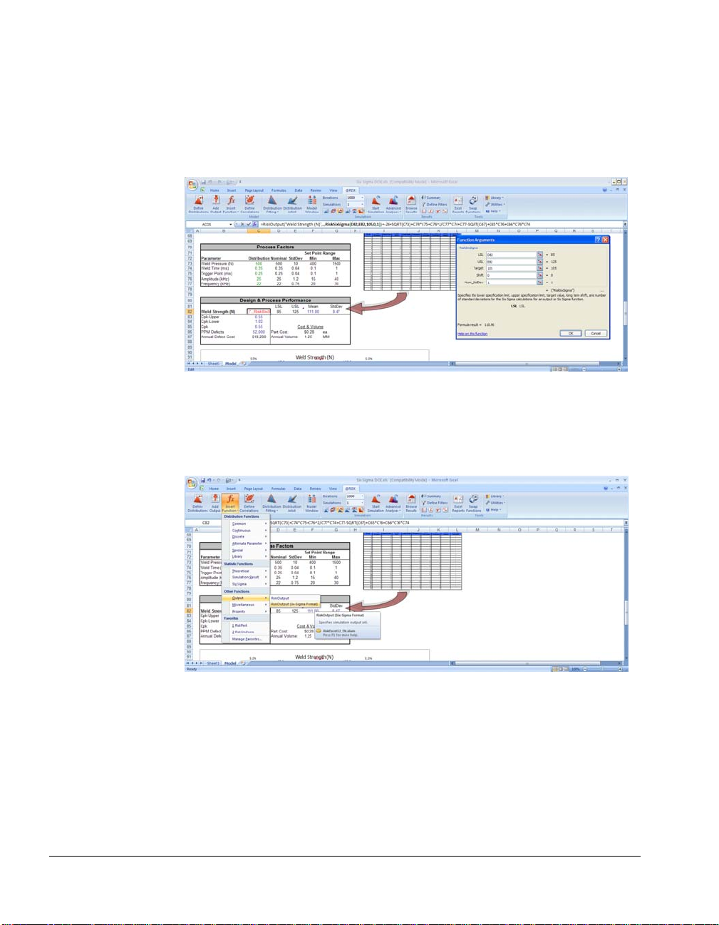
The Six Sigma Output
The output is Weld Strength (N) in the Design & Process
Performance section, and contains a RiskSixSigma property
function that includes the Lower Specification Limit (LSL), Upper
Specification Limit (USL), and Target value specified. As with
defining input distributions, you can type the output formula
directly in the output cell or use the Add Output dialog. The
formula would be:
=RiskOutput("Weld Strength (N)",,,RiskSixSigma(D82,E82,105,0,1))+
[the mathematical calculation]
Case Studies 49
Page 56

The Add Output dialog appears below:
Clicking on the properties button (fx) brings up the Output
Properties dialog with the Six Sigma tab. Here you can enter
LSL, USL, Target value, and other Six Sigma properties for
your output. These are used to calculate Six Sigma statistics.
50 Example 2 – Design of Experiments: Welding
Page 57

Simulation Results
After you run the simulation, Six Sigma statistics were generated
using @RISK Six Sigma functions for Cpk-Upper, Cpk-Lower,
Cpk, and PPM Defects (or DPM). Standard @RISK statistics
functions (like RiskMean) were also used.
The @RISK output distribution displays the expected
performance based on the design and process input variation and
shows LSL, USL, and Target value with markers. You can easily
access the output statistics using the reporting features or through
@RISK functions.
Case Studies 51
Page 58

The @RISK Sensitivity Analysis clearly shows that the Weld Time
and Amplitude parameters are driving the Weld Strength
variation.
The next steps for this problem could include two options: The
engineer can attempt to reduce or better control the variation
within the Weld Time and Amplitude, or use RISKOptimizer to
find the optimal process and design targets to maximize yield or
reduce scrap cost.
52 Example 2 – Design of Experiments: Welding
Page 59

Example 3 – Design of Experiments with Optimization
Example Model: Six Sigma DOE Opt.xls
This model demonstrates the use of RISKOptimizer in experimental
design. RISKOptimizer combines Monte Carlo simulation with
genetic algorithm-based optimization. Using these two techniques,
RISKOptimizer is uniquely capable of solving complex optimization
problems that involve uncertainty.
With RISKOptimizer, you can choose to maximize, minimize, or
approach a target value for any given output in your model.
RISKOptimizer tries many different combinations of controllable
inputs that you specify in an effort to reach its goal. Each
combination is called a “solution,” and the total group of solutions
tried is called the “population.” “Mutation” refers to the process of
randomly trying new solutions unrelated to previous trials. You can
also set constraints that RISKOptimizer must abide by during the
optimization.
For uncertain, uncontrollable factors in your model, you define
@RISK probability distribution functions. For each trial combination
of inputs, RISKOptimizer also runs a Monte Carlo simulation,
sampling from those @RISK functions and recording the output for
that particular trial. RISKOptimizer can run thousands of trials to get
you the best possible answer. By accounting for uncertainty,
RISKOptimizer is far more accurate than standard optimization
programs.
In this example, as above, the part under investigation is a metallic
burst cup manufactured by welding a disk onto a ring. The product
functions as a seal and a safety device, so it must hold pressure in
normal use, and it must separate if the internal pressure exceeds the
safety limit.
The model relates the weld strength to process and design factors,
models the variation for each factor, and forecasts the product
performance. RISKOptimizer was used to search for the optimal
combination of process settings and nominal design values to
minimize scrap cost, called Annual Defect Cost in the model. This is
the same as maximizing yield.
Case Studies 53
Page 60

The process and design variables RISKOptimizer will adjust are:
Design Variables
• Disk thickness
• Horn wall thickness
• Horn length
Process Variables
• Weld pressure
• Weld time
• Trigger point
• Amplitude
• Frequency
All in an effort to minimize the output Annual Defect Cost.
54 Example 3 – Design of Experiments with Optimization
Page 61

RISKOptimizer Toolbar
The RISKOptimizer toolbar added to Excel 2000-2003 appears below:
Model RISKOptimizer Start Reports Utilities
Settings Optimization
The RISKOptimizer toolbar in Excel 2007 appears as follows:
Case Studies 55
Page 62

The Optimization Model
Clicking on the Model Definition icon brings up the following
dialog where you define which cells to adjust, what your output
is, and what constraints to use. In addition to the inputs and
outputs described above, we will also define a constraint where
the Trigger Point must always be less than or equal to Weld Time.
56 Example 3 – Design of Experiments with Optimization
Page 63

Optimization Settings
Clicking on Optimization Settings icon brings up the following
dialog where you can set a variety of conditions for how the
optimization and simulations will run.
Case Studies 57
Page 64

Running the Optimization
When you click Start Optimization, the RISKOptimizer Progress
window appears, showing you a summary status of the analysis.
The magnifying glass button opens the RISKOptimizer Watcher
dialog, which displays more detailed information about the
optimization and simulations being run. Below you can see a
chart of simulations run and best values obtained.
58 Example 3 – Design of Experiments with Optimization
Page 65

The Summary tab displays Best, Original, and Last values calculated,
as well as parameters for the optimization like Crossover and
Mutation Rates.
The Diversity tab visually shows the different cells being calculated
and the various possible solutions.
After simulation and optimization, RISKOptimizer efficiently
found a solution that reduced the Annual Defect Cost to under
$8,000.
Using RISKOptimizer can save time and resources in a quality
improvement and cost reduction effort. The next steps for this
problem would be to validate the model and optimized solution
through experimentation.
Case Studies 59
Page 66

60 Example 3 – Design of Experiments with Optimization
Page 67

Example 4 – DFSS: Electrical Design
Example Model: Six Sigma Electrical Design.xls
This simple DC circuit consists of two voltage sources - one independent
and one dependent - and two resistors. The independent source specified
by the design engineer has an operational power range of 5,550 W + 300
W. If the power draw on the independent voltage source is outside of the
specification, the circuit will be defective. The design performance results
clearly indicate that the design is not capable of performance with a
percentage of the circuits failing on both the high and low end of the
limits. The PNC values identify the Percent of Nonconforming units
expected on the upper and lower ends of the specification.
The basic model logic follows:
Inputs
VI
VD
R1
R2
Power Supply
(Independent)
Outputs
Transfer Function
(V=IR, P=VI)
PI
Resistors
Power Supply
(Dependent)
Vs
+
R1
R2
XiVs = i
Case Studies 61
Page 68

The model calculates the standard deviation for each component
based on known information and the following assumptions within
this model:
1) The mean of the component values are centered within the
tolerance limits.
2) The component values are normally distributed. Note that
@RISK can be used to fit a probability distribution to a data
set or to model other types of probability distributions, if
needed.
A RiskSixSigma property function in the Output cell PowerDEP
defines Upper Limit, Lower Limit, and Target that are used for Six
Sigma results calculations. @RISK Six Sigma functions are used to
calculate Cpk Lower, Cpk Upper, Cpk, Cp, DPM, PNC Upper and
PNC Lower.
Sensitivity Analysis
The @RISK Sensitivity Analysis identifies the input variables driving
variation in the output. The sensitivity shows that the two voltage
sources are the main contributors to the variation in power
consumption. Armed this information, the engineering team can
focus their improvement efforts on the voltage sources instead of the
resistors.
The model can be used to test different components and tolerances,
performances and yields can be compared, and the optimal solution
can be selected to maximize yield and reduce cost.
62 Example 4 – DFSS: Electrical Design
Page 69

Example 5 – Lean Six Sigma:
Analysis of Current State –
Quotation Process
Example Model: Six Sigma Quotation Process.xls
In both Lean and Six Sigma approaches to continuous improvement,
one of the key requirements is to understand the current state of the
process under review. This is initially done in the Value Stream
Mapping phase of a Lean Implementation or in the Define and
Measure phases of the DMAIC Six Sigma process. Most practitioners
put the process together in one or more sessions and, after a cursory
review, the team moves on to generating solutions. There is
significant benefit, however to taking the time to model the process
and prove that the data and assumptions that were made are accurate.
This becomes vitally important when one or more of the following are
true:
• The process is critical to the success of the enterprise (Mission
Critical)
• There is significant denial that the process needs improvement
• Improvement costs will be significant
• The results of the continuous improvement effort may come
under significant scrutiny at a later date
• The process is subject to the Hawthorne Effect – the more we
study it, the better it gets
Simulation has the ability to prove the initial analysis of the current
state and show the true situation that the analysis team encountered.
There are three often very different processes at work in every area:
the process that we think exists; the process we have documented;
and the process that really is being carried out on a daily basis. A
carefully constructed @RISK simulation can document the actual
process and model the impact of improvements later in the
Continuous Improvement cycle. And the model is straightforward to
construct.
Case Studies 63
Page 70

Developing the Model and Collecting Data
This example focuses on the process flow of an organization’s
internal sales quotation process, and was taken from an actual
company. There are many tools used to graphically show the
process. The one we will use here is a Swimlane Chart.
The entire quotation process had over 36 individual steps and
was impacted by ten individuals or departments. Cursory data
indicated that it took up to four weeks to get the quote through
the system, yet for critical issues, quotes could be expedited
through the system in less than one week. Long quote cycletimes
prevented the company from effective bidding in often lucrative
emergency orders for their products and services. Because of the
fact that expedited quotes could be done in one quarter of the
time, management thought that the issue resided in the personnel,
not the process. The analysis team needed a tool to prove the
process was at fault.
After developing the chart, the team had a question: How long
does it take to process a quotation from the receipt of the request
to the release of the quote package to the Engineering
department? This is the first part of the process and had data that
was relatively easy to acquire, and findings here could be applied
throughout the process.
64 Example 5 – Lean Six Sigma: Analysis of Current State – Quotation Process
Page 71

This portion of the quotation process has four steps. First, the data is
collected and entered (Step A). Next, it goes into a queue for
Customer Service review (Step B). Here, corrections and additional
data are entered onto the form and tracking number assigned (Step
C). Finally the packet is put into a queue for the Engineering
department to perform the quotation activity (Step D).
The team developed a simple time sheet that captured the times that
the paperwork went from area to area, and how long it was worked
on in each step of the process. From this data, the team performed
some initial analysis of the four steps in this portion of the process.
Case Studies 65
Page 72

Building the Distributions and Defining the Output
A simple distribution of the data, for our purposes, means that
the data follows a single curve. Complex distributions are made
up of several separate distributions and are typically more
difficult to define. The data that the team gathered has both
types.
@RISK can find the distribution behind the data through the Fit
Distributions button on the toolbar. A fitted distribution can
then be entered as a distribution function in the spreadsheet.
With your data in Excel, select the Fit Distributions button and
follow the prompts. @RISK will analyze the data and check its fit
to a series of distribution functions.
For the team’s data on Step C (Review), the result from @RISK’s
distribution fitting is shown below. The resulting distribution
was then placed directly into the spreadsheet cell below the “CReview” heading using the Write to Cell button. (The team
selected the Normal distribution over the slightly better fitting
Weibull because, with a small dataset, the difference between the
two curves was acceptable.)
66 Example 5 – Lean Six Sigma: Analysis of Current State – Quotation Process
Page 73

The team continued to do this for all the distributions for each of the
four steps. Finally they set the Total Time for the four Steps A-D as
the @RISK output and ran the simulation.
The results of the simulation were revealing. The mean Total Time to
process a quote was about 1700 minutes, which is over one calendar
day. It could take anywhere from 350 minutes (almost 6 hours) to
well over 2 calendar days.
The only value-added portion of the time is the Review step. This
step took an average of 35 minutes to complete, with a range of from 6
to 64 minutes. This was reviewed with the area affected and
management, though surprised, agreed with the findings.
Statistics on Simulation Results
@RISK also allowed the team to generate basic statistics that interact
with the output cell. As an example, the team wanted to add the
mean, maximum, minimum and standard deviation of the Total Time
output cell to a table in the spreadsheet. From @RISK’s Insert
Function menu, the team selected Simulation Result in the Statistics
section. From this set, the RiskMean function was chosen. Finally the
output cell “Total Time” was selected as the argument. Now every
time the simulation is run, this cell is updated with the mean of the
Total Time.
The team repeated this for the maximum, minimum, and standard
deviation selections.
Case Studies 67
Page 74

Entering Six Sigma Functions
Next the team wanted to add the Cpk analysis of the output cell
using the @RISK Six Sigma functions. In the output cell Total
Time, they entered a RiskSixSigma function, where:
• a cell reference identified the the header cell where the name
of the output was taken
• a cell reference identified the Lower Specification Limit for
the expected result
• a cell reference identified the Upper Specification Limit for
the expected result
• a cell reference identified the Target value for the expected
result
The RiskSixSigma function was easily set up using the Output
Properties dialog (accessed by clicking the Function Properties fx
icon in @RISK’s Add/Edit Output dialog).
68 Example 5 – Lean Six Sigma: Analysis of Current State – Quotation Process
Page 75

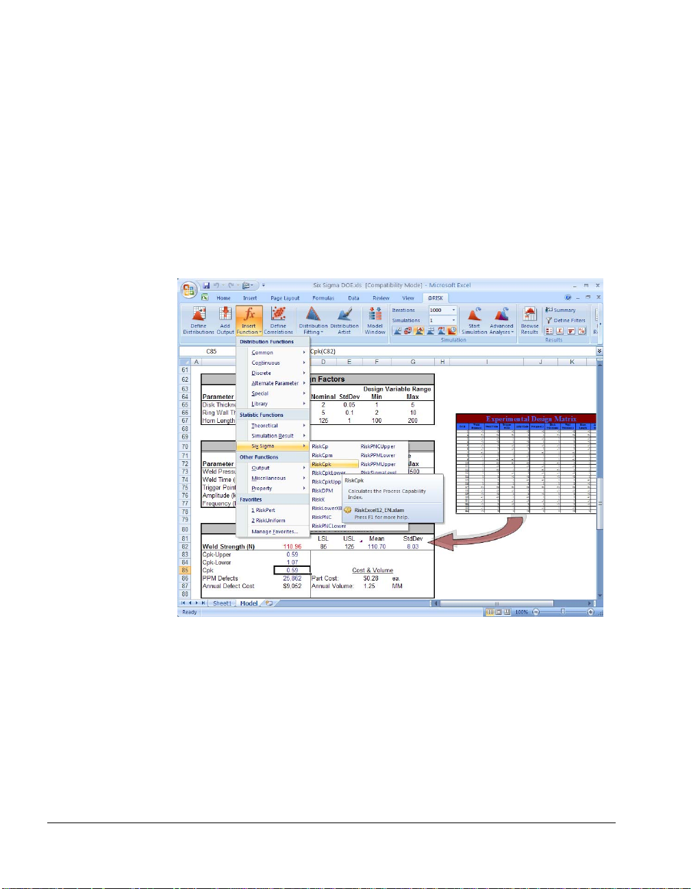
With the output now configured, the team wanted the simulation to
calculate the @RISK Six Sigma functions of Cp, CpkUpper,
CpkLower and Cpk. This is done by inserting the correct function
(such as RiskCp, RiskCpkUpper, etc) from Six Sigma in the Statistics
section of @RISK’s Insert Function menu or by typing them into the
formula bar. These will be recalculated for every simulation.
Case Studies 69
Page 76

Graphing the Simulation Output
Through @RISK’s results graphs and Six Sigma markers showing
LSL, USL, and Target values directly on the graph, management
was surprised to see that it took, on average, over a full day to
complete 35 minutes of work. The simulation results for the Total
Time output, and for the values sampled from the input
distribution fo Step C – Review are shown below.
70 Example 5 – Lean Six Sigma: Analysis of Current State – Quotation Process
Page 77

The team could, based on the simulation, document the actual
flows and detail what happens when the quotes are not
expedited. Management saw the potential improvement if the
entire process were tracked and improved. This management
buy-in at the project onset proved to be key to the long term
success of the project.
From this initial model, the team constructed the full model for
the entire process. With this model in hand, the team was able to
model improvement efforts at various stages of the project and
verify that the improvements were making positive gains. The
total time to generate the initial simulation and results using
@RISK was less than one hour after the original data was entered
into Excel.
Case Studies 71
Page 78

72 Example 5 – Lean Six Sigma: Analysis of Current State – Quotation Process
Page 79

Example 6 – DMAIC: Roll Through Yield Analysis
Example Model: Six Sigma DMAIC RTY.xls
DMAIC - or Define, Measure, Analyze, Improve, and Control - is
used to improve existing products or processes. Imagine you are a
costume jewelry manufacturer, coating inexpensive silver with thin
layers of gold. You import materials and components from China. A
small number of components are always defective, but you don't
know how many or how much it is costing.
You've gathered data on the number of components that are defective
or become defective at various points in the manufacturing process.
On the surface, it seems like defective parts are not a major problem.
Upwards of 99% of components are acceptable at each stage of the
process. However, the combined effect of the defective parts leads to
15-20% waste of final products, which can translate into 200,000
defective units per million produced. If materials are $.50 per unit,
that is $100,000 in waste before counting labor, machine time, and
other expenses.
Case Studies 73
Page 80

You need to reduce the number of defective units produced.
However, the process is long and complicated, and you don't know
which stage to begin with. Using @RISK, you can simulate many
different outcomes and pinpoint the manufacturing stage that is the
worst offender. You can also get key process capability metrics for
each stage as well as the entire process that will help you improve
quality and reduce waste. In this way, @RISK is being used in the
Measure and Analyze phases of the DMAIC method. @RISK is used
to measure the existing state of the process (with capability metrics)
and analyze how it might be improved (with sensitivity analysis).
Distribution Fitting
Using the data gathered from the manufacturing process, @RISK's
distribution fitting feature was used to define distribution functions
describing the number of defective parts at each stage of the process Unpackaging/Inspection, Cutting, Cleaning, and Electroplating.
The distribution fit for the Electroplating phase – Weibull distribution
- is shown below.
74 Example 6 – DMAIC: Roll Through Yield Analysis
Page 81

Simulation Results
These fitted distributions were added directly to the model. The
Electroplating distribution is shown below.
The Defective Parts per Million (DPPM) for each stage, and the
process as a whole, were defined as @RISK outputs with Six Sigma
specifications for Upper Specification Limit, Lower Specification
Limit, and Target values. After the simulation run, a variety of Six
Sigma metrics were calculated for each stage and the process as a
whole.
Case Studies 75
Page 82

The distribution of outcomes for DPPM is shown below.
Finally, sensitivity analysis and a Tornado graph revealed that the
Cutting stage was the most to blame for overall product defects,
despite the fact that another stage - Cleaning - had a lower First Time
Yield (fewer defects). Even though the FTY of Cutting was higher, the
Cutting process itself is less consistent and has more variation than
the other processes.
76 Example 6 – DMAIC: Roll Through Yield Analysis
Page 83

Example 7 – Vendor Selection
Example Model: Six Sigma Vendor Selection.xls
Imagine you are launching a new product. During the
implementation phase of product launch your company predicts
selling 25,000 units per month. A critical component of your product
is outsourced for precision machining. That is, this component must
meet very specific requirements in order to be used in your product.
In particular, the length of this component must be 66.6 mm, with a
tolerance of only +/- 1 mm.
Three vendors currently supply the critical component. You have
negotiated a different unit price for the component with each vendor.
However, the quality of the component varies with each vendor.
Some of the supplied components are not within the specified length.
With two of the vendors, you must inspect all incoming components
to verify they are within specification. This adds labor and scrap cost
to the process. The third vendor is certified, and guarantees 100% of
the components will be within specification, eliminating the need for
inspection and scrap. However, the unit price from this vendor is
highest of the three.
You will always need multiple vendors in case one goes down.
However, you want to know which vendor has the highest real cost
per unit so that you can develop a more efficient strategy for sourcing
your components.
Case Studies 77
Page 84

Modeling Component Length
Component length for each vendor is described by @RISK
distribution functions. These cells are also defined as @RISK outputs
with RiskSixSigma functions to enable us to calculate Cpm for each
vendor as well as generate distribution graphs of the component
lengths with specification markers. The RiskSixSigma functions
contain the USL, LSL, and Target value of 66.6 mm, with a tolerance
of only +/- 1 mm.
Component Specifications (mm)
LSL Target USL
66.5 66.6 66.7
For example, the component length for Vendor 1 is described by a
Pert distribution, and contains RiskSixSigma properties:
= RiskOutput(,,,RiskSixSigma(B30,D30,C30,0,6))+RiskPert(66.4,66.6,66.7)
78 Example 7 – Vendor Selection
Page 85

Simulation Results
After simulating, you see that Vendor 1 has the lowest real unit cost.
The simulated mean of each vendor's unit cost is displayed as well, by
using a RiskMean function. Finally, the Cpm is calculated for the
component length of each vendor.
Real Total Cost
of Good
Components
(per unit)
Cpm Length
Mean of Real Total Cost
per unit
Vendor 1 $6.13 0.553 $6.16
Vendor 2 $6.75 0.472 $7.03
Vendor 3
(certified)
$6.40 0.686 $6.40
The variation around the quality of Vendor 1 is illustrated in the
graph below.
You now have information on cost and quality to form a more
efficient ordering strategy. A next step might be to analyze how to
further reduce costs, for example using a Kaizen event to reduce
internal inspection time.
Case Studies 79
Page 86

80 Example 7 – Vendor Selection
Page 87

Example 8 – Six Sigma DMAIC Failure Rate
Example Model: Six Sigma DMAIC Failure.xls
This is a failure rate model for use in quality control and planning.
You are a manufacturer and need to calculate the likely % of defective
products. In the DMAIC method - Define Measure, Analyze,
Improve, Control - this is the Measure and Analyze phases, where
you wish to measure the current state of quality and analyze the
causes of problems or defects.
A product is defective when any one of its components does not meet
its required tolerance level. Each component is deemed to be
satisfactory if some property of its finished state (e.g. its width) lies
within the defined tolerance bands.
Case Studies 81
Page 88

Modeling Component Width
This property of each finished component (e.g. its width) is modeled
with a Normal distribution in the Sample column.
Sample
10.00
5.00
8.00
12.00
6.00
Those cells have also been added as @RISK outputs with
RiskSixSigma property functions defining LSL, USL, and Target
values for each component. The formula for Component1 appears
below:
=RiskOutput(,,,RiskSixSigma(F26,G26,C26,0,0))+RiskNormal(C26,D26)
In this way we'll be able to see graphs of the components’ quality, and
calculate Six Sigma statistics on each component.
82 Example 8 – Six Sigma DMAIC Failure Rate
Page 89

Using the RiskMean Function to Get Failure Rate
The component and aggregate Failure Rate is calculated from the
RiskMean function, which is an @RISK Statistics function, and
therefore applicable only after the simulation has been run. After
simulation we can also see component and aggregate Six Sigma
statistics Z score and DPM.
Z Min Failure frequency DPM
2.999060375 One in 334 will fail 3000
2.99523275 One in 334 will fail 3000
2.990852805 One in 334 will fail 3000
3.492267357 One in 1000 will fail 1000
3.002125568 One in 1000 will fail 1000
2.945880756 One in 91 will fail 11000
The graph for the samples of Component1 appears below, with
markers for USL, LSL, and Target.
Case Studies 83
Page 90

84 Example 8 – Six Sigma DMAIC Failure Rate
Page 91

Example 9 – Six Sigma DMAIC Failure Rate using RiskTheo
Example Model: Six Sigma DMAIC Failure RiskTheo.xls
This is an extension of the DMAIC Failure model for use in quality
control and planning. It includes the use of RiskTheo functions (in this
case RiskTheoXtoP) for determining failure rate without actually
running a simulation. RiskTheo functions return theoretical statistics
on input distributions or formulas rather than returning the statistics
on the data from a simulation run.
You are a manufacturer and need to calculate the likely % of defective
products. In the DMAIC method - Define Measure, Analyze,
Improve, Control - this is the Measure and Analyze phases, where
you wish to measure the current state of quality and analyze the
causes of problems or defects.
A product is defective when any one of its components does not meet
its required tolerance level. Each component is deemed to be
satisfactory if some property of its finished state (e.g. its width) lies
within the defined tolerance bands.
Case Studies 85
Page 92

Modeling Component Width
This property of each finished component (e.g. its width) is modeled
with a Normal distribution in the Sample column.
Sample
10.00
5.00
8.00
12.00
6.00
Those cells have also been added as @RISK outputs with
RiskSixSigma property functions defining LSL, USL, and Target
values for each component. The formula for Component1 appears
below:
=RiskOutput(,,,RiskSixSigma(F26,G26,C26,0,0))+RiskNormal(C26,D26)
In this way we'll be able to see graphs of the components' quality and
calculate Six Sigma statistics on each component if we choose to run a
simulation.
86 Example 9 – Six Sigma DMAIC Failure Rate using RiskTheo
Page 93

Using the RiskTheoXtoP Function to Get Failure Rate
The component and aggregate Failure Rate is calculated from the
RiskTheoXtoP, which draws on the Normal distributions in the
Sample column. The Failure Rate from simulation is also calculated
using the RiskMean function if you choose to run a simulation. In this
way you can compare simulated Failure Rate with RiskTheo Failure
Rate.
Failure rate
(%) from sim
(%)
Failure rate from
RiskTheo (%)
0.30% 0.270%
0.20% 0.158%
0.20% 0.138%
0.00% 0.047%
0.10% 0.135%
1%
After simulation we can also see component and aggregate Six Sigma
statistics Z score and DPM.
Z Min from sim
DPM from
sim
2.998616548 3000
2.997415317 2000
2.997730848 2000
3.49840855 0
3.004560454 1000
3.146403741 8000
Case Studies 87
Page 94

88 Example 9 – Six Sigma DMAIC Failure Rate using RiskTheo
 Loading...