Palisade RISK 4.5 User Manual

Guide to Using

@RISK

Risk Analysis and Simulation

®

Add-In for Microsoft

Version 4.5

June, 2005

Excel

Palisade Corporation
798 Cascadilla St.
Ithaca, NY USA 14850
[phone]
[phone] (fax)
http://www.palisade.com (website)
[e-mail] (e-mail)

Copyright Notice

Copyright © 2005, Palisade Corporation.

Trademark Acknowledgments

Microsoft, Excel and Windows are registered trademarks of Microsoft, Inc.
IBM is a registered trademark of International Business Machines, Inc.
Palisade, TopRank, BestFit and RISKview are registered trademarks of Palisade
Corporation.
RISK is a trademark of Parker Brothers, Division of Tonka Corporation and is used under
license.

Welcome

@RISK for Microsoft Excel

Welcome to @RISK, the revolutionary software system for the
analysis of business and technical situations impacted by risk! The
techniques of Risk Analysis have long been recognized as powerful
tools to help decision-makers successfully manage situations subject
to uncertainty. Their use has been limited because they have been
expensive, cumbersome to use, and have substantial computational
requirements. However, the growing use of computers in business
and science has offered the promise that these techniques can be
commonly available to all decision-makers.

That promise has been finally realized with @RISK (pronounced "at
risk") — a system which brings these techniques to the industry
standard spreadsheet package, Microsoft Excel. With @RISK and
Excel any risky situation can be modeled, from business to science
and engineering. You are the best judge of what your analysis needs
require, and @RISK, combined with the modeling capabilities of
Excel, allows you to design a model which best satisfies those needs.
Anytime you face a decision or analysis under uncertainty, you can
use @RISK to improve your picture of what the future could hold.

Why You Need Risk Analysis and @RISK

Traditionally, analyses combine single "point" estimates of a model's
variables to predict a single result. This is the standard Excel model
— a spreadsheet with a single estimate of results. Estimates of model
variables must be used because the values which actually will occur
are not known with certainty. In reality, however, many things just
don't turn out the way that you have planned. Maybe you were too
conservative with some estimates and too optimistic with others. The
combined errors in each estimate often lead to a real-life result that is
significantly different from the estimated result. The decision you
made based on your "expected" result might be the wrong decision,
and a decision you never would have made if you had a more
complete picture of all possible outcomes. Business decisions,
technical decisions, scientific decisions ... all use estimates and
assumptions. With @RISK, you can explicitly include the uncertainty
present in your estimates to generate results that show all possible
outcomes.

Welcome i

@RISK uses a technique called "simulation" to combine all the
uncertainties you identify in your modeling situation. You no longer
are forced to reduce what you know about a variable to a single
number. Instead, you include all you know about the variable,
including its full range of possible values and some measure of
likelihood of occurrence for each possible value. @RISK uses all this
information, along with your Excel model, to analyze every possible
outcome. It's just as if you ran hundreds or thousands of "what-if"
scenarios all at once! In effect, @RISK lets you see the full range of
what could happen in your situation. It's as if you could "live"
through your situation over and over again, each time under a
different set of conditions, with a different set of results occurring.

All this added information sounds like it might complicate your
decisions, but in fact, one of simulation's greatest strengths is its
power of communication. @RISK gives you results that graphically
illustrate the risks you face. This graphical presentation is easily
understood by you, and easily explained to others.

So when should you use @RISK? Anytime you make an analysis in
Excel that could be affected by uncertainty, you can and should use
@RISK. The applications in business, science and engineering are
practically unlimited and you can use your existing base of Excel
models. An @RISK analysis can stand alone, or be used to supply
results to other analyses. Consider the decisions and analyses you
make every day! If you've ever been concerned with the impact of
risk in these situations, you've just found a good use for @RISK!

Modeling Features

As an "add-in" to Microsoft Excel, @RISK "links" directly to Excel to
add Risk Analysis capabilities. The @RISK system provides all the
necessary tools for setting up, executing and viewing the results of
Risk Analyses. And @RISK works in a style you are familiar with —
Excel style menus and functions.

@RISK Functions

ii Welcome

@RISK allows you to define uncertain cell values in Excel as
probability distributions using functions. @RISK adds a set of new
functions to the Excel function set, each of which allows you to
specify a different distribution type for cell values. Distribution
functions can be added to any number of cells and formulas
throughout your worksheets and can include arguments which are
cell references and expressions — allowing extremely sophisticated
specification of uncertainty. To help you assign distributions to
uncertain values, @RISK includes a graphical pop-up window where
distributions can be previewed and added to formulas.

Available Distribution Types

The probability distributions provided by @RISK allow the
specification of nearly any type of uncertainty in cell values in your
spreadsheet. A cell containing the distribution function
NORMAL(10,10), for example, would return samples during a
simulation drawn from a normal distribution (mean = 10, standard
deviation = 10). Distribution functions are only invoked during a
simulation — in normal Excel operations, they show a single cell
value — just the same as Excel before @RISK. Available distribution
types include:

Beta BetaGeneral Beta-Subjective
Binomial Chi-Square Cumulative
Discrete Discrete Uniform Error Function
Erlang Exponential Extreme Value
Gamma General Geometric
Histogram Hypergeometric Inverse Gaussian
IntUniform Logistic Log-Logistic
Lognormal Lognormal2 Negative Binomial
Normal Pareto Pareto2
Pearson V Pearson VI PERT
Poisson Rayleigh Student's t
Triangular Trigen Uniform
Weibull

All distributions may be truncated to allow only samples within a
given ranges of values within the distribution. Also, many
distributions can also use alternate percentile parameters. This allows
you to specify values for specific percentile locations of an input
distribution as opposed to the traditional arguments used by the
distribution.

@RISK Simulation Analysis

@RISK has sophisticated capabilities for specifying and executing
simulations of Excel models. Both Monte Carlo and Latin Hypercube
sampling techniques are supported, and distributions of possible
results may be generated for any cell or range of cells in your
spreadsheet model. Both simulation options and the selection of
model outputs are entered with Windows style menus, dialog boxes
and use of the mouse.

Graphics

High resolution graphics are used to present the output distributions
from your @RISK simulations. Histograms, cumulative curves and
summary graphs for cell ranges all lead to a powerful presentation of
results. And all graphs may be displayed in Excel for further
enhancement and hard copy. An essentially unlimited number of
output distributions may be generated from a single simulation —
allowing for the analysis of even the largest and most complex
spreadsheets!

Welcome iii

Advanced Simulation Capabilities

The options available for controlling and executing a simulation in
@RISK are among the most powerful ever available. They include:

• Latin Hypercube or Monte Carlo sampling

• Any number of iterations per simulation

• Any number of simulations in a single analysis

• Animation of sampling and recalculation of the spreadsheet

• Seeding the random number generator

• Real time results and statistics during a simulation

High Resolution Graphic Displays

Product Execution Speed

@RISK graphs a probability distribution of possible results for each
output cell selected in @RISK. @RISK graphics include:

• Relative frequency distributions and cumulative probability

curves

• Summary graphs for multiple distributions across cell ranges

(for example, a worksheet row or column)

• Statistical reports on generated distributions

• Probability of occurrence for target values in a distribution

• Export of graphics as Windows metafiles for further

enhancement

Execution time is of critical importance because simulation is
extremely calculation intensive. @RISK is designed for the fastest
possible simulations through the use of advanced sampling
techniques.

iv Welcome

Table of Contents

Chapter 1: Getting Started 1

Introduction.........................................................................................3

Installation Instructions.....................................................................7

Quick Start.........................................................................................11

Chapter 2: An Overview to Risk Analysis 15

Introduction.......................................................................................17

What Is Risk? ....................................................................................19

What Is Risk Analysis? ....................................................................23

Developing an @RISK Model...........................................................25

Analyzing a Model with Simulation.................................................27

Making a Decision: Interpreting the Results.................................29

What Risk Analysis Can (Cannot) Do.............................................33

Chapter 3: Upgrade Guide 35

Introduction.......................................................................................37

New @RISK Model Window.............................................................39

New @RISK Add-in Features...........................................................43

New @RISK Results Window ..........................................................45

New Features in @RISK 4.5 vs @RISK 4.0.....................................49

Table of Contents v

Chapter 4: Getting to Know @RISK 57

A Quick Overview to @RISK...........................................................59

Setting Up and Simulating an @RISK Model.................................69

Chapter 5: @RISK Modeling Techniques 91

Introduction ...................................................................................... 93

Modeling Interest Rates and Other Trends ...................................95

Projecting Known Values into the Future...................................... 97

Modeling Uncertain or "Chance" Events.......................................99

Oil Wells and Insurance Claims....................................................101

Adding Uncertainty Around a Fixed Trend..................................103

Dependency Relationships ...........................................................105

Sensitivity Simulation....................................................................107

Simulating a New Product: The Hippo Example.........................109

Finding Value at Risk (VAR) of a Portfolio .................................. 119

Simulating the NCAA Tournament...............................................123

Chapter 6: Distribution Fitting 127

Overview ......................................................................................... 129

Define Input Data............................................................................131

Select Distributions To Fit............................................................. 135

Run The Fit......................................................................................139

Interpret the Results ......................................................................143

Using the Results of a Fit..............................................................151

vi Table of Contents

Chapter 7: @RISK Reference Guide 153

Introduction.....................................................................................161

Reference: @RISK Icons................................................................163

Reference: @RISK Add-In Menu Commands 173

File Menu .........................................................................................175

Model Menu.....................................................................................177

Simulate Menu ................................................................................189

Results Menu ..................................................................................203

Options Menu..................................................................................207

Advanced Analyses Menu .............................................................209

Goal Seek.........................................................................................211

Stress Analysis...............................................................................217

Advanced Sensitivity Analysis......................................................229

Reference: @RISK Model Window Commands 247

File Menu .........................................................................................249

Edit Menu.........................................................................................251

View Menu .......................................................................................253

Insert Menu......................................................................................255

Simulation Menu.............................................................................263

Model Menu.....................................................................................265

Correlation Menu............................................................................275

Fitting Menu.....................................................................................283

Graph Menu.....................................................................................309

Table of Contents vii

Artist Menu......................................................................................317

Window Menu .................................................................................323

Help Menu.......................................................................................325

Reference: @RISK Results Window Commands 327

File Menu.........................................................................................329

Edit Menu ........................................................................................331

View Menu.......................................................................................335

Insert Menu.....................................................................................337

Simulation Menu.............................................................................353

Results Menu.................................................................................. 355

Graph Menu .................................................................................... 361

Window Menu .................................................................................379

Help Menu.......................................................................................381

Reference: @RISK Functions 383

Introduction .................................................................................... 383

Reference: Distribution Functions...............................................401

Reference: Distribution Property Functions...............................429

Reference: Output Functions........................................................439

Reference: Statistics Functions ...................................................441

Reference: Supplemental Functions............................................ 447

Reference: Graphing Function ..................................................... 449

Reference: @RISK Macros 451

Overview ......................................................................................... 451

viii Table of Contents

Using VBA to Modify @RISK Settings and Enter Outputs.........453

Using VBA to Run Simulations, Get Results and Generate

Reports.........................................................................................455

Using VBA to Run Advanced Analyses........................................457

Appendix A: Sampling Methods 459

What is Sampling?..........................................................................459

Appendix B: Using @RISK With Other DecisionTools® 465

The DecisionTools Suite................................................................465

Palisade’s DecisionTools Case Study..........................................467

Introduction to TopRank®..............................................................471

Using @RISK with TopRank..........................................................475

Introduction to PrecisionTree™.....................................................479

Using @RISK with PrecisionTree..................................................483

Appendix C: Glossary 487

Appendix D: Recommended Readings 493

Readings by Category....................................................................493

Table of Contents ix

x Table of Contents

Chapter 1: Getting Started

Introduction.........................................................................................3

Checking Your Package ..........................................................................3

About This Version .................................................................................3

Working with your Operating Environment ......................................4

If You Need Help .....................................................................................4

@RISK System Requirements................................................................6

Installation Instructions.....................................................................7

General Installation Instructions..........................................................7

The DecisionTools Suite.........................................................................8

Setting Up the @RISK Icons or Shortcuts............................................9

Macro Security Warning Message on Startup ....................................9

Quick Start.........................................................................................11

On-line Tutorial......................................................................................11

Starting On Your Own ..........................................................................11

Quick Start with Your Own Spreadsheets ........................................12

Using @RISK 4.5 Spreadsheets in @RISK 3.5 or earlier..................13

Using @RISK 4.5 Spreadsheets in @RISK 4.0...................................13

@RISK 4.5 Help System © Palisade Corporation, 1999

Chapter 1: Getting Started 1

2 @RISK for Microsoft Excel

Introduction

This introduction describes the contents of your @RISK package and
shows you how to install @RISK and attach it to your copy of Microsoft
Excel 97 for Windows or higher.

Checking Your Package

Your @RISK package should contain:

The @RISK User’s Guide (this book) with:

• Getting Started

• Overview to Risk Analysis and @RISK

• Upgrade Guide

• Getting to Know @RISK

• @RISK Modeling Techniques

• Distribution Fitting

• @RISK Reference Guide

• Technical Appendices

The @RISK CD-ROM including:

• @RISK Program

• @RISK Tutorial

The @RISK Licensing Agreement

A complete listing of all files contained on the @RISK CD is contained in
the file INSTALL.LOG found in the PROGRAM FILES\PALISADE
\RISK45 directory on your hard disk.

If your package is not complete, please call your @RISK dealer or supplier
or contact Palisade Corporation directly at [phone]. If you want to
install @RISK from diskettes, please contact Palisade Corporation.

About This Version

This version of @RISK can be installed as a 32-bit program for Microsoft
Excel 97 or higher.

Chapter 1: Getting Started 3

Working with your Operating Environment

This User’s Guide assumes that you have a general knowledge of the
Windows operating system and Excel. In particular:

• You are familiar with your computer and using the mouse.

• You are familiar with terms such as icons, click, double-click, menu, window,

command and object.

• You understand basic concepts such as directory structures and file naming.

If You Need Help

Technical support is provided free of charge for all registered users of
@RISK with a current maintenance plan, or is available on a per incident
charge. To ensure that you are a registered user of @RISK, please register
online at www.palisade.com/html/register.html.

If you contact us by telephone, please have your serial number and User’s
Guide ready. We can offer better technical support if you are in front of
your computer and ready to work.

Before Calling

Before contacting technical support, please review the following checklist:

• Have you referred to the on-line help?

• Have you checked this User's Guide and reviewed the on-line multimedia

tutorial?

• Have you read the README.WRI file? It contains current information on

@RISK that may not be included in the manual.

• Can you duplicate the problem consistently? Can you duplicate the problem

on a different computer or with a different model?

• Have you looked at our site on the World Wide Web? It can be found at

http://www.palisade.com. Our Web site also contains the latest FAQ (a
searchable database of tech support questions and answers) and @RISK
patches in our Technical Support section. We recommend visiting our Web
site regularly for all the latest information on @RISK and other Palisade
software.

4 Introduction

Contacting Palisade

Palisade Corporation welcomes your questions, comments or suggestions
regarding @RISK. Contact our technical support staff using any of the
following methods:

• E-mail us at [e-mail].

• Telephone us at [phone] any weekday from 9:00 AM to 5:00 PM,

EST. Press 2 on a touch-tone phone to reach technical support.

• Fax us at [phone].

• Mail us a letter at:

Technical Support
Palisade Corporation
798 Cascadilla St
Ithaca, NY 14850 USA

If you want to contact Palisade Europe:

• E-mail us at [e-mail].

• Telephone us at +44 (0)2074269950 (UK).

• Fax us at +44(0)2073751229 (UK).

• Mail us a letter at:

Palisade Europe
Technical Support
The Blue House, Unit 1
30 Calvin Street
London E1 6NW UK

If you want to contact Palisade Asia-Pacific:

• E-mail us at [e-mail]

• Telephone us at +61299299799 (AU).

• Fax us at +61299543882(AU).

• Mail us a letter at:

Palisade Asia-Pacific Pty Limited
Suite 101, Level 1
8 Cliff Street
Milsons Point NSW 2061
AUSTRALIA

Regardless of how you contact us, please include the product name, exact
version and serial number. The exact version can be found by by selecting
the Help About command on the @RISK menu in Excel.

Chapter 1: Getting Started 5

Student Versions

Telephone support is not available with the student version of @RISK. If
you need help, we recommend the following alternatives:

• Consult with your professor or teaching assistant.

• Log-on to our site on the World Wide Web for answers to frequently asked

questions.

• Contact our technical support department via e-mail or fax.

@RISK System Requirements

System requirements for @RISK 4.5 for Microsoft Excel for Windows
include:

• Pentium PC or faster with a hard disk.

• Microsoft Windows 98 or higher or Windows NT 4.0 or higher.

• Microsoft Excel Version 97 or higher.

6 Introduction

Installation Instructions

General Installation Instructions

The Setup program copies the @RISK system files into a directory you
specify on your hard disk. Setup asks you for the location of the Excel
directory on your hard disk, so please note this information before
running Setup. Setup and @RISK require Microsoft Windows to run, so
be sure to start Windows before running these programs.

To run the Setup program in Windows 98 or higher:

1) Insert the @RISK CD-ROM in your CD-ROM drive

2) Click the Start button, click Settings and then click Control Panel

3) Double-click the Add/Remove Programs icon

4) On the Install/Uninstall tab, click the Install button

5) Follow the Setup instructions on the screen

If you encounter problems while installing @RISK, verify that there is
adequate space on the drive to which you’re trying to install. After
you’ve freed up adequate space, try rerunning the installation.

Authorizing Your Copy of @RISK

Chapter 1: Getting Started 7

Within 30 days of installing @RISK you need to authorize your copy of
@RISK.

Authorization can be done over the Internet by clicking the Authorize
Now button and following the prompts on the screen. Alternatively, you
can contact Palisade or Palisade Europe during normal business hours
and authorize your copy of @RISK over the phone.

An authorized copy of @RISK is licensed for use on a single computer
only. If you wish to move your copy of @RISK to a different computer,
please contact Palisade for instructions.

Removing @RISK from Your Computer

The DecisionTools Toolbar

Setup creates the file INSTALL.LOG in your @RISK directory. This file
lists the names and locations of all installed files. If you wish to remove
@RISK from your computer, use the Control Panel’s Add/Remove
Programs utility and select the entry for @RISK.

The DecisionTools Suite

@RISK for Excel is a member of the DecisionTools Suite, a set of products
for risk and decision analysis described in Appendix D: Using @RISK
With Other DecisionTools. The default installation procedure of @RISK
puts @RISK in a subdirectory of a main “Program Files\Palisade”
directory. This is quite similar to how Excel is often installed into a
subdirectory of a “Microsoft Office” directory.

One subdirectory of the Program Files\Palisade directory will be the
@RISK directory (by default called RISK45). This directory contains the
@RISK program files (RSKMODEL.EXE and RSKRSLTS.EXE) plus
example models and other files necessary for @RISK to run. Another
subdirectory of Program Files\Palisade is the SYSTEM directory which
contains files which are needed by every program in the DecisionTools
Suite, including common help files and program libraries.

When you launch one of the elements of the Suite (such as @RISK) from
its desktop icon, Excel will load a “DecisionTools Suite” toolbar which
contains one icon for each program of the Suite. This allows you to
launch any of the other products in the suite directly from Excel.

Note: In order for TopRank, the what-if analysis program in the
DecisionTools Suite, to work properly with @RISK, you must have
release TopRank 1.5e or higher.

8 Installation Instructions

Setting Up the @RISK Icons or Shortcuts

Creating the Shortcut in the Windows Taskbar

In Windows, setup automatically creates an @RISK command in the
Programs menu of the Taskbar. However, if problems are encountered
during Setup, or if you wish to do this manually another time, follow the
following directions.

1) Click the Start button, and then point to Settings.

2) Click Taskbar, and then click the Start Menu Programs tab.

3) Click Add, and then click Browse.

4) Locate the file RISK.EXE and double click it.

5) Click Next, and then double-click the menu on which you want the

program to appear.

6) Type the name “@RISK”, and then click Finish.

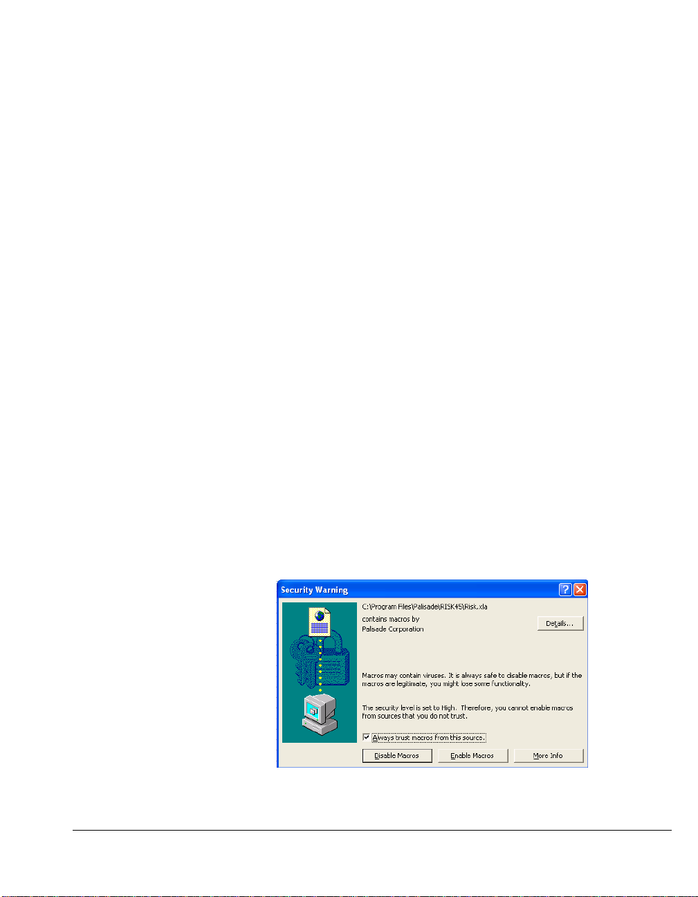
Macro Security Warning Message on Startup

Microsoft Office provides several security settings (under
Tools>Macro>Security) to keep unwanted or malicious macros from
being run in Office applications. A warning message appears each time
you attempt to load a file with macros, unless you use the lowest security
setting. To keep this message from appearing every time you run a
Palisade add-in, Palisade digitally signs their add-in files. Thus, once you
have specified Palisade Corporation as a trusted source, you can open
any Palisade add-in without warning messages. To do this:

• Click Always trust macros from this source when a Security

Warning dialog (such as the one below) is displayed when
starting @RISK.

Chapter 1: Getting Started 9

10 Installation Instructions

Quick Start

On-line Tutorial

In the on-line tutorial, @RISK experts guide you through sample models
in

streaming .WMV movie format. This tutorial is a multi-media

presentation on the main features of @RISK.

The system requirements for the tutorial are:

• Windows Media Player plug-in

• A computer with audio capability

The tutorial can be run by selecting the Start Menu/ Programs/ Palisade
DecisionTools/ Tutorials/ @RISK Tutorial and clicking on the file
RISK45.html.

Starting On Your Own

If you're in a hurry, or just want to explore @RISK on your own, here's a
quick way to get started.

After attaching @RISK according to the Installation instructions outlined
previously in this section:

1) Click the @RISK icon in the Windows Start Programs Palisade

DecisionTools group. If the Security Warning dialog is displayed, follow
the instructions in the section "Setting Palisade as a Trusted Source" in
this chapter.

2) Use the Excel Open command to open the example spreadsheet

FINANCE.XLS. The default location for the examples is
C:\PROGRAM FILES\PALISADE\RISK45\EXAMPLES.

3) Click the List icon on the @RISK Toolbar — the one on the Toolbar with

the red and blue arrow. The Outputs and Inputs list, listing the
distribution functions in the FINANCE worksheet along with your
output cell C10, NPV at 10%, is displayed.

4) Click the "Simulate" icon — the one with the red distribution curve.

You've just started a risk analysis on NPV for the FINANCE
worksheet. The Simulation analysis is underway. When it is complete,
your risk analysis results will be displayed.

Chapter 1: Getting Started 11

To make graphs for Risk Analysis results:

1) When results are shown, right click on the name of an output or input in

the Explorer list and select Histogram. A graph of simulation results for
the highlighted output or input cell will be displayed.

2) To modify a graph, click the right mouse button when the cursor is

located over the graph window. Select Graph Format from the pop-up
menu.

For all analyses, if you want to see @RISK "animate" its operation during
the simulation, turn the Simulation Settings dialog box Update Display
check box on or press the <Num Lock> key during the simulation. @RISK
then will show you how it changes your spreadsheet iteration by iteration
and generates results.

Quick Start with Your Own Spreadsheets

Working through the @RISK On-Line Tutorial and reading the @RISK
Reference Guide is the best method for preparing to use @RISK on your
own spreadsheets. However, if you're in a hurry, or just don't want to
work through the Tutorial, here is a quick step-by-step guide to using
@RISK with your own spreadsheets:

1) Click the @RISK icon in the Windows Start Programs Palisade

DecisionTools group.

2) If necessary, use the Excel Open command to open your spreadsheet

3) Examine your spreadsheet and locate those cells where uncertain

assumptions or inputs are located. You will substitute @RISK
distribution functions for these values.

4) Enter distribution functions for the uncertain inputs which reflect the

range of possible values and their likelihood of occurrence. Start with
the simple distribution types — such as UNIFORM, which just requires
a minimum and maximum possible value, or TRIANG which just
requires a minimum, most likely and maximum possible value.

5) Once you've entered your distributions, select the spreadsheet cell or

cells for which you wish to get simulation results and click the "Add
Output" icon — the one with the single red arrow — on the @RISK
Toolbar.

To run a simulation:

1) Click the "Simulate" icon — the one with the red distribution curve —

on the @RISK Toolbar. A simulation of your spreadsheet will be
executed and results displayed.

12 Quick Start

Using @RISK 4.5 Spreadsheets in @RISK 3.5 or earlier

@RISK 4.5 spreadsheets can only be used in @RISK 3.5 or earlier when the
simple forms of distribution functions are used. In the simple distribution
function format only required distribution parameters can be used. No
new @RISK 4.5 distribution property functions can be added. In addition,
RiskOutput functions must be removed and outputs reselected when
simulating in @RISK 3.5.

Using @RISK 4.5 Spreadsheets in @RISK 4.0

@RISK 4.5 spreadsheets can be used directly in @RISK 4.0 with the
following exceptions:

 Alternate Parameter functions, such as RiskNormalAlt, will not

work and will return an error.

 Cumulative Descending functions, such as RiskCumulD, will

not work and will return an error.

Chapter 1: Getting Started 13

14 Quick Start

Chapter 2: An Overview to Risk Analysis

Introduction.......................................................................................17

What Is Risk? ....................................................................................19

Characteristics of Risk...........................................................................19

The Need for Risk Analysis.................................................................20

Assessing and Quantifying Risk.........................................................21

Describing Risk with a Probability Distribution ............................22

What Is Risk Analysis? ....................................................................23

Developing an @RISK Model...........................................................25

Variables..................................................................................................25

Output Variables....................................................................................26

Analyzing a Model with Simulation.................................................27

Simulation ...............................................................................................27

How Simulation Works ........................................................................28

The Alternative to Simulation.............................................................28

Making a Decision: Interpreting the Results.................................29

Interpreting a Traditional Analysis....................................................29

Interpreting an @RISK Analysis.........................................................29

Individual Preference............................................................................30

The Distribution "Spread"....................................................................30

Skewness .................................................................................................32

What Risk Analysis Can (Cannot) Do.............................................33

Chapter 2: An Overview to Risk Analysis 15

16 Quick Start

Introduction

@RISK brings advanced modeling and Risk Analysis to Microsoft Excel.
You might wonder if what you do qualifies as modeling and/or would be
suitable for Risk Analysis. If you use data to solve problems, make
forecasts, develop strategies, or make decisions, then you definitely
should consider doing Risk Analysis.

Modeling is a catch-all phrase that usually means any type of activity
where you are trying to create a representation of a real life situation so
you can analyze it. Your representation, or model, can be used to examine
the situation, and hopefully help you understand what the future might
bring. If you've ever played "what-if" games with your project by
changing the values of various entries, you are well on your way to
understanding the importance of uncertainty in a modeling situation.

Okay, so you do analyses and make models — what is involved in
making these analyses and models explicitly incorporate risk? The
following discussion will try to answer this question. But don't worry,
you don't have to be an expert in statistics or decision theory to analyze
situations under risk, and you certainly don't have to be an expert to use
@RISK. We can't teach you everything in a few pages, but we'll get you
started. Once you begin using @RISK you'll automatically begin picking
up the type of expertise that can't be learned from a book.

Another purpose of this chapter is to give you an overview of how @RISK
works with your spreadsheet to perform analyses. You don't have to
know how @RISK works to use it successfully, but you might find some
explanations useful and interesting. This chapter discusses:

• What risk is and how it can be quantitatively assessed.

• The nature of Risk Analysis and the techniques used in @RISK.

• Running a simulation.

• Interpreting @RISK results.

• What Risk Analysis can and cannot do.

Chapter 2: An Overview to Risk Analysis 17

18 Introduction

What Is Risk?

Everyone knows that "risk" affects the gambler about to roll the dice, the
wildcatter about to drill an oil well, or the tightrope walker taking that
first big step. But these simple illustrations aside, the concept of risk
comes about due to our recognition of future uncertainty — our inability
to know what the future will bring in response to a given action today.
Risk implies that a given action has more than one possible outcome.

In this simple sense, every action is "risky", from crossing the street to
building a dam. The term is usually reserved, however, for situations
where the range of possible outcomes to a given action is in some way
significant. Common actions like crossing the street usually aren't risky
while building a dam can involve significant risk. Somewhere in
between, actions pass from being nonrisky to risky. This distinction,
although vague, is important — if you judge that a situation is risky, risk
becomes one criterion for deciding what course of action you should
pursue. At that point, some form of Risk Analysis becomes viable.

Characteristics of Risk

Risk derives from our inability to see into the future, and indicates a
degree of uncertainty that is significant enough to make us notice it. This
somewhat vague definition takes more shape by mentioning several
important characteristics of risk.

First, risk can be either objective or subjective. Flipping a coin is an
objective risk because the odds are well known. Even though the
outcome is uncertain, an objective risk can be described precisely based
on theory, experiment, or common sense. Everyone agrees with the
description of an objective risk. Describing the odds for rain next
Thursday is not so clear cut, and represents a subjective risk. Given the
same information, theory, computers, etc., weatherman A may think the
odds of rain are 30% while weatherman B may think the odds are 65%.
Neither is wrong. Describing a subjective risk is open-ended in the sense
that you could always refine your assessment with new information,
further study, or by giving weight to the opinion of others. Most risks are
subjective, and this has important implications for anyone analyzing risk
or making decisions based on a Risk Analysis.

Chapter 2: An Overview to Risk Analysis 19

Second, deciding that something is risky requires personal judgment,
even for objective risks. For example, imagine flipping a coin where you
win $1 for a heads and lose $1 for a tails. The range between $1 and -$1
would not be overly significant to most people. If the stakes were
$100,000 and -$100,000 respectively, most people would find the situation
to be quite risky. There would be a wealthy few, however, who would
not find this range of outcomes to be significant.

Third, risky actions and therefore risk are things that we often can choose
or avoid. Individuals differ in the amount of risk they willingly accept.
For example, two individuals of equal net worth may react quite
differently to the $100,000 coin flip bet described above — one may accept
it while the other refuses it. Their personal preference for risk differs.

The Need for Risk Analysis

The first step in Risk Analysis and modeling is recognizing a need for it.
Is there significant risk involved in the situation you are interested in?
Here are a few examples that might help you evaluate your own
situations for the presence of significant risk:

• Risks for New Product Development and Marketing — Will the

R&D department solve the technical problems involved? Will a competitor
get to market first, or with a better product? Will government regulations
and approvals delay product introduction? How much impact will the
proposed advertising campaign have on sales levels? Will production costs
be as forecast? Will the proposed sales price have to be changed to reflect
unanticipated demand levels for the product?

• Risks for Securities Analysis and Asset Management — How will a

tentative purchase affect portfolio value? Will a new management team
affect market price? Will an acquired firm add earnings as forecast? How
will a market correction impact a given industry sector?

• Risks for Operations Management and Planning — Will a given

inventory level suffice for unpredictable demand levels? Will labor costs rise
significantly with upcoming union contract negotiations? How will pending
environmental legislation impact production costs? How will political and
market events affect overseas suppliers in terms of exchange rates, trade
barriers, and delivery schedules?

• Risks for Design and Construction of a Structure (building, bridge,

dam,...) — Will the cost of construction materials and labor be as forecast?

Will a labor strike affect the construction schedule? Will the levels of stress
placed on the structure by peak load crowds and nature be as forecast? Will
the structure ever be stressed to the point of failure?

20 What Is Risk?

• Risks for Investment in Exploration for Oil and Minerals — Will

anything be found? If a deposit is found, will it be uneconomical, or a
bonanza? Will the costs of developing the deposit be as forecast? Will some
political event like an embargo, tax reform, or new environmental regulations
drastically alter the economic viability of the project?

• Risks for Policy Planning — If the policy is subject to legislative

approval, will it be approved? Will the level of compliance with any policy
directives be complete or partial? Will the costs of implementation be as
forecast? Will the level of benefits be what you projected?

Assessing and Quantifying Risk

The first step in Risk Analysis and modeling is recognizing a need for it.
Is there significant risk involved in the situation you are interested in?
Here are a few examples that might help you evaluate your own
situations for the presence of significant risk.

Realizing that you have a risky situation is only the first step. How do
you quantify the risk you have identified for a given uncertain situation?
"Quantifying risk" means determining all the possible values a risky
variable could take and determining the relative likelihood of each value.
Suppose your uncertain situation is the outcome from the flip of a coin.
You could repeat the flip a large number of times until you had
established the fact that half of the times it comes up tails and half of the
times heads. Alternatively, you could mathematically calculate this result
from a basic understanding of probability and statistics.

In most real life situations, you can't perform an "experiment" to calculate
your risk the way you can for the flip of a coin. How could you calculate
the probable learning curve associated with introducing new equipment?
You may be able to reflect on past experiences, but once you have
introduced the equipment, the uncertainty is gone. There is no
mathematical formula that you can solve to get the risk associated with
the possible outcomes. You have to estimate the risk using the best
information you have available.

If you can calculate the risks of your situation the way you would for a
coin flip, the risk is objective. This means that everyone would agree that
you quantified the risk correctly. Most risk quantification, however,
involves your best judgment.

Chapter 2: An Overview to Risk Analysis 21

There may not be complete information available about the situation, the
situation may not be repeatable like a coin flip, or it just may be too
complex to come up with an unequivocal answer. Such risk
quantification is subjective, which means that someone might disagree
with your evaluation.

Your subjective assessments of risk are likely to change when you get
more information on the situation. If you have subjectively derived a risk
assessment, you must always ask yourself whether additional information
is available that would help you make a better assessment. If it is
available, how hard and how expensive would it be to obtain? How
much would it cause you to change the assessment you already have
made? How much would these changes affect the final results of any
model you are analyzing?

Describing Risk with a Probability Distribution

If you have quantified risk — determined outcomes and probabilities of
occurrence — you can summarize this risk using a probability
distribution. A probability distribution is a device for presenting the
quantified risk for a variable. @RISK uses probability distributions to
describe uncertain values in your Excel worksheets and to present results.
There are many forms and types of probability distributions, each of
which describes a range of possible values and their likelihood of
occurrence. Most people have heard of a normal distribution — the
traditional "bell curve". But there is a wide variety of distribution types
ranging from uniform and triangular distributions to more complex forms
such as gamma and weibull.

All distribution types use a set of arguments to specify a range of actual
values and distribution of probabilities. The normal distribution, for
example, uses a mean and standard deviation as its arguments. The mean
defines the value around which the bell curve will be centered and the
standard deviation defines the range of values around the mean. Over
thirty types of distributions are available to you in @RISK for describing
distributions for uncertain values in your Excel worksheets.

The @RISK Define Distribution window allows you to graphically
preview distributions and assign them to uncertain values. Using its
graphs, you can quickly see the range of possible values your distribution
describes.

22 What Is Risk?

What Is Risk Analysis?

In a broad sense, Risk Analysis is any method — qualitative and/or
quantitative — for assessing the impacts of risk on decision situations.
Myriad techniques are used that blend both qualitative and quantitative
techniques. The goal of any of these methods is to help the decision­maker choose a course of action, given a better understanding of the
possible outcomes that could occur.

Risk Analysis in @RISK is a quantitative method that seeks to determine
the outcomes of a decision situation as a probability distribution. In
general, the techniques in an @RISK Risk Analysis encompass four steps:

• Developing a Model — by defining your problem or situation in Excel

worksheet format

• Identifying Uncertainty — in variables in your Excel worksheet and

specifying their possible values with probability distributions, and
identifying the uncertain worksheet results you want analyzed

• Analyzing the Model with Simulation — to determine the range and

probabilities of all possible outcomes for the results of your worksheet

• Making a Decision — based on the results provided and personal

preferences

@RISK helps with the first three steps, by providing a powerful and
flexible tool that works with Excel to facilitate model building and Risk
Analysis. The results that @RISK generates can then be used by the
decision-maker to help choose a course of action.

Fortunately, the techniques @RISK employs in a Risk Analysis are very
intuitive. As a result, you won't have to accept our methodology on faith.
And you won't have to shrug your shoulders and resort to calling @RISK
a "black box" when your colleagues and superiors query you as to the
nature of your Risk Analysis. The discussion to follow will give you a
firm understanding of just what @RISK needs from you in the way of a
model, and how an @RISK Risk Analysis proceeds.

Chapter 2: An Overview to Risk Analysis 23

24 What Is Risk Analysis?

Developing an @RISK Model

You are the "expert" at understanding the problems and situations that
you would like to analyze. If you have a problem that is subject to risk,
then @RISK and Excel can help you construct a complete and logical
model.

A major strength of @RISK is that it allows you to work in a familiar and
standard model building environment — Microsoft Excel. @RISK works
with your Excel model, allowing you to conduct a Risk Analysis, but still
preserves the familiar spreadsheet capabilities. You presumably know
how to build spreadsheet models in Excel — @RISK now gives you the
ability to easily modify these models for Risk Analysis.

Variables

Variables are the basic elements in your Excel worksheets that you have
identified as being important ingredients to your analysis. If you are
modeling a financial situation, your variables might be things like Sales,
Costs, Revenues or Profits whereas if you are modeling a geologic
situation, your variables might be things like Depth to Deposit, Thickness
of Coal Seam or Porosity. Each situation has its own variables, identified
by you. In a typical worksheet, a variable labels a worksheet row or
column, for example:

Certain or Uncertain

Chapter 2: An Overview to Risk Analysis 25

You may know the values your variables will take in the time frame of
your model — they are certain, or what statisticians call "deterministic".
Conversely, you may not know the values they will take — they are
uncertain, or "stochastic". If your variables are uncertain you will need to
describe the nature of their uncertainty. This is done with probability
distributions, which give both the range of values that the variable could
take (minimum to maximum), and the likelihood of occurrence of each
value within the range. In @RISK, uncertain variables and cell values are
entered as probability distribution functions, for example:

RiskNormal(100,10)

RiskUniform(20,30)

RiskExpon(A1+A2)

RiskTriang(A3/2.01,A4,A5)

These "distribution" functions can be placed in your worksheet cells and
formulas just like any other Excel function.

Independent or Dependent

In addition to being certain or uncertain, variables in a Risk Analysis
model can be either "independent" or "dependent". An independent
variable is totally unaffected by any other variable within your model.
For example, if you had a financial model evaluating the profitability of
an agricultural crop, you might include an uncertain variable called
Amount of Rainfall. It is reasonable to assume that other variables in your
model such as Crop Price and Fertilizer Cost would have no effect on the
amount of rain — Amount of Rainfall is an independent variable.

A dependent variable, in contrast, is determined in full or in part by one
or more other variables in your model. For example, a variable called
Crop Yield in the above model should be expected to depend on the
independent variable Amount of Rainfall. If there's too little or too much
rain, then the crop yield is low. If there's an amount of rain that is about
normal, then the crop yield would be anywhere from below average to
well above average. Maybe there are other variables that affect Crop
Yield such as Temperature, Loss to Insects, etc.

When identifying the uncertain values in your Excel worksheet, you have
to decide whether your variables are correlated. These variables would
all be “correlated” with each other. The Corrmat function in @RISK is
used to identify correlated variables. It is extremely important to correctly
recognize correlations between variables or your model might generate
nonsensical results. For example, if you ignored the relationship between
Amount of Rainfall and Crop Yield, @RISK might choose a low value for
the rainfall at the same time it picked a high value for the crop yield —
clearly something nature wouldn't allow.

Output Variables

Any model needs both input values and output results, and a Risk
Analysis model is no different. An @RISK Risk Analysis generates results
on cells in your Excel worksheet. Results are probability distributions of
the possible values which could occur. These results are usually the same
worksheet cells that give you the results of a regular Excel analysis —
Profit, the "bottom line" or other such worksheet entries.

26 Developing an @RISK Model

Analyzing a Model with Simulation

Once you have placed uncertain values in your worksheet cells and have
identified the outputs of your analysis, you have an Excel worksheet that
@RISK can analyze.

Simulation

@RISK uses simulation, sometimes called Monte Carlo simulation, to do a
Risk Analysis. Simulation in this sense refers to a method whereby the
distribution of possible outcomes is generated by letting a computer
recalculate your worksheet over and over again, each time using different
randomly selected sets of values for the probability distributions in your
cell values and formulas. In effect, the computer is trying all valid
combinations of the values of input variables to simulate all possible
outcomes. This is just as if you ran hundreds or thousands of "what-if"
analyses on your worksheet, all in one sitting.

What is meant by saying that simulation "tries all valid combinations of
the values of input variables"? Suppose you have a model with only two
input variables. If there is no uncertainty in these variables, you can
identify a single possible value for each variable. These two single values
can be combined by your worksheet formulas to calculate the results of
interest — also a certain or deterministic value. For example, if the certain
input variables are:

Revenues = 100
Costs = 90

then the result

Profits = 10

would be calculated by Excel from

Profits = 100 - 90

There is only one combination of the input variable values, because there
is only one value possible for each variable.

Now consider a situation where there is uncertainty in both input
variables. For example,

Revenues = 100 or 120
Costs = 90 or 80

gives two values for each input variable. In a simulation, @RISK would
consider all possible combinations of these variable values to calculate
possible values for the result, Profits.

Chapter 2: An Overview to Risk Analysis 27

There are four combinations:

Profits = Revenues - Costs
10 = 100 - 90
20 = 100 - 80
30 = 120 - 90
40 = 120 - 80

Profits also is an uncertain variable because it is calculated from uncertain
variables.

How Simulation Works

In @RISK, simulation uses two distinct operations:

• Selecting sets of values for the probability distribution functions contained in the

cells and formulas of your worksheet

• Recalculating the Excel worksheet using the new values

The selection of values from probability distributions is called sampling and each
calculation of the worksheet is called an iteration.

The following diagrams show how each iteration uses a set of single values
sampled from distribution functions to calculate single-valued results. @RISK
generates output distributions by consolidating single-valued results from all the
iterations.

The Alternative to Simulation

There are two basic approaches to quantitative Risk Analysis. Both have the
same goal — to derive a probability distribution that describes the possible
outcomes of an uncertain situation — and both generate valid results. The first
approach is the one just described for @RISK, namely, simulation. This approach
relies on the ability of the computer to do a great deal of work very quickly —
solving your worksheet repeatedly using a large number of possible
combinations of input variable values.

The second approach to Risk Analysis is an analytical approach. Analytical
methods require that the distributions for all uncertain variables in a model be
described mathematically. Then the equations for these distributions are
combined mathematically to derive another equation, which describes the
distribution of possible outcomes. This approach is not practical for most uses
and users. It is not a simple task to describe distributions as equations, and it is
even more difficult to combine distributions analytically given even moderate
complexity in your model. Furthermore, the mathematical skills necessary to
implement the analytical techniques are significant.

28 Analyzing a Model with Simulation

Making a Decision: Interpreting the Results

@RISK analysis results are presented in the form of probability
distributions. The decision-maker must interpret these probability
distributions, and make a decision based on the interpretation. How do
you interpret a probability distribution?

Interpreting a Traditional Analysis

Let's start by looking at how a decision-maker would interpret a single­valued result from a traditional analysis — an "expected" value. Most
decision-makers compare the expected result to some standard or
minimum acceptable value. If it's at least as good as the standard, they
find the result acceptable. But, most decision-makers recognize that the
expected result doesn't show the impacts of uncertainty. They have to
somehow manipulate the expected result to make some allowance for
risk. They might arbitrarily raise the minimum acceptable result, or they
might non rigorously weigh the chances that the actual result could
exceed or fall short of the expected result. At best, the analysis might be
extended to include several other results — such as "worst case" and "best
case" — in addition to the expected value. The decision-maker then
decides if the expected and "best case" values are good enough to
outweigh the "worst case" value.

Interpreting an @RISK Analysis

In an @RISK Risk Analysis, the output probability distributions give the
decision-maker a complete picture of all the possible outcomes. This is a
tremendous elaboration on the "worst-expected-best" case approach
mentioned above. But the probability distribution does a lot more than
just fill in the gaps between these three values:

• Determines a "Correct" Range — Because you have more rigorously

defined the uncertainty associated with every input variable, the possible
range of outcomes may be quite different from a "worst case-best case" range
— different, and more correct.

• Shows Probability of Occurrence — A probability distribution shows

the relative likelihood of occurrence for each possible outcome.

As a result, you no longer just compare desirable outcomes with undesirable
outcomes. Instead, you can recognize that some outcomes are more likely to
occur than others, and should be given more weight in your evaluation. This
process also is a lot easier to understand than the traditional analysis because
a probability distribution is a graph — you can see the probabilities and get a
feel for the risks involved.

Chapter 2: An Overview to Risk Analysis 29

Individual Preference

The results provided by an @RISK analysis must be interpreted by you as
an individual. The same results given to different individuals may be
interpreted differently, and lead to different courses of action. This is not
a weakness in the technique, but a direct result of the fact that different
individuals have different preferences with regard to possible choices,
time, and risk. You might feel that the shape of the output distribution
shows that the chances of an undesirable outcome far outweigh the
chances of a desirable outcome. A colleague who is less risk averse might
come to the opposite conclusion.

The Distribution "Spread"

Range and likelihood of occurrence are directly related to the level of risk
associated with a particular event. By looking at the spread and
likelihood of possible results, you can make an informed decision based
on the level of risk you are willing to take. Risk averse decision-makers
prefer a small spread in possible results, with most of the probability
associated with desirable results. But if you are a risk-taker, then you will
accept a greater spread or possible variation in your outcome distribution.
Furthermore, a risk-taker will be influenced by "bonanza" outcomes even
if their likelihood of occurrence is small.

Regardless of your personal risk preferences, there are some general
conclusions about riskiness that apply to all decision-makers. The
following probability distributions illustrate these conclusions:

Probability distribution A represents greater risk than B despite identical shapes
because the range of A includes less desirable results — the spread relative to the
mean is greater in A than B.

A

-10 0 10

30 Making a Decision: Interpreting the Results

B

90 100 110

Probability distribution C represents greater risk than D because the probability
of occurrence is uniform across the range for C whereas it is concentrated around
98 for D.

C

90 100 110

D

90 100 110

Probability distribution F represents greater risk than E because the range is
larger and the probability of occurrence is more spread out than for E.

E

F

90 100 110

90 100 110

Chapter 2: An Overview to Risk Analysis 31

Skewness

A simulation output distribution also can show skewness — how much
the distribution of possible results deviates from being symmetrical.
Suppose your distribution had a large positive 'tail'. If you saw only a
single number for the expected result, you might not realize the
possibility of a highly positive outcome that could occur in the tail.
Skewness such as this can be very important to decision makers. By
presenting all the information, @RISK "opens up" a decision by showing
you all possible outcomes.

32 Making a Decision: Interpreting the Results

What Risk Analysis Can (Cannot) Do

Quantitative analysis techniques have gained a great deal of popularity
with decision-makers and analysts in recent years. Unfortunately, many
people have mistakenly assumed that these techniques are magic "black
boxes" that unequivocally arrive at the correct answer or decision. No
technique, including those used by @RISK, can make that claim. These
techniques are tools that can be used to help make decisions and arrive at
solutions. Like any tools, they can be used to good advantage by skilled
practitioners, or they can be used to create havoc in the hands of the
unskilled. In the context of Risk Analysis, quantitative tools should never
be used as a replacement for personal judgment.

Finally, you should recognize that Risk Analysis cannot guarantee that the
action you choose to follow — even if skillfully chosen to suit your
personal preferences — is the best action viewed from the perspective of
hindsight. Hindsight implies perfect information, which you never have
at the time the decision is made. You can be guaranteed, however, that
you have chosen the best personal strategy given the information that is
available to you. That's not a bad guarantee!

Chapter 2: An Overview to Risk Analysis 33

34 What Risk Analysis Can (Cannot) Do

Chapter 3: Upgrade Guide

Introduction.......................................................................................37

Key Features............................................................................................37

New @RISK Model Window.............................................................39

Defining Probability Distributions in your Spreadsheet...............40

Review Distributions in the @RISK Model Window .....................41

Using Data to Define Probability Distributions..............................42

New @RISK Add-in Features...........................................................43

New Menus, Icons and Commands....................................................43

New and Enhanced @RISK Functions in Excel................................43

New @RISK Results Window ..........................................................45

New Results Window Options............................................................45

Other Enhancements .............................................................................47

New Features in @RISK 4.5 vs @RISK 4.0.....................................49

Advanced Analyses................................................................................50

Alternate Parameters for Probability Distributions........................52

Cumulative Descending Percentiles...................................................53

Quick Reports.........................................................................................54

Enhanced Define Distribution Window............................................55

Improved Error Reporting....................................................................56

Chapter 3: Upgrade Guide 35

36 What Risk Analysis Can (Cannot) Do

Introduction

@RISK 4.5 and its predecessor, @RISK 4.0, are major upgrades to earlier
versions of @RISK. @RISK 4.5 brings together features of its companion
programs BestFit and RISKview to provide a fully functional risk analysis
environment, while maintaining compatibility with earlier versions of
@RISK. It also offers enhanced integration with Microsoft Excel to give
easier access to simulation results directly in your spreadsheet. @RISK 4.5
is available in three versions – Standard, Professional and Industrial – to
allow you to select the feature set you need.

Key Features

Key features of @RISK 4.5 include:

•

Fully integrated RISKview (for distribution viewing) in all the

•

Fully integrated BestFit (for distribution fitting) in the Professional

•

Fully integrated RISKOptimizer (for Simulation Optimization) in the

Note: RISKview, BestFit and RISKOptimizer are also available as stand­alone programs.

versions.

and Industrial versions.

Industrial version.

• New toolbars, graphs and “Explorer” interface

•

Improved integration with Excel with new functions and new

reporting in Excel

Improved performance with faster loading and simulation

•

•

Full compatibility with existing @RISK models and functions

Key enhancements of @RISK 4.5 vs. @RISK 4.0 include:

•

Three new analyses – Goal Seek, Stress Analysis and Advanced

Sensitivity Analysis – for advanced investigations on @RISK models

(Professional and Industrial versions only)

•

Alternate parameters (such as percentiles) can be used for defining

many distribution types, and the distribution functions in Excel have
been added that support alternate parameters

•

Quick reports, designed for printing, for quick, single page reports on

simulation results

•

Integrated support for multiple CPUs in a single PC for high-speed

simulations through parallel processing (Industrial version only)

Chapter 3: Upgrade Guide 37

• Enhanced Define Distribution window, including pop-up

distribution pallette, intelligent default parameters, easy entry of
Excel cell references and more

•

Other enhancements, including improved filtering, report formatting

and more

Note: The information provided in this chapter is designed for users
familiar with earlier versions of @RISK. New users should skip this
chapter and continue with Chapter 4: Getting to Know @RISK to gain a
full understanding of the operation and features of @RISK 4.5.

Three Main Components of @RISK 4.5

@RISK 4.5 is comprised of three main components:

1)

@RISK Model window for listing inputs and outputs, viewing input

distributions, fitting distributions, and defining correlations. @RISK
Model also allows the pop-up graphical definition of distributions for
components of cell formulas.

2)

@RISK add-in to Excel, including new menus and icons, new

distribution functions, new statistics functions, new output functions,
and new simulation reports in Excel.

3)

@RISK Results window for interactive graphs of simulation results,

statistics, data, sensitivity and scenario reports.

Each of the three components share a common user interface including an
“Explorer-style” listing of simulation inputs and outputs and
customizable toolbars and icons.

38 Introduction

New @RISK Model Window

A new @RISK Model Window provides an entire set of options for
assigning and viewing probability distributions used in your spreadsheet
model, correlating them, and fitting distributions to data. This window
allows you to handle all the tasks necessary for setting up your @RISK
model prior to simulating it.

Chapter 3: Upgrade Guide 39

Pop-Up Window for Assigning Distributions

Defining Probability Distributions in your Spreadsheet

With @RISK 4.5 you can easily assign probability distributions to
uncertain values in your spreadsheet model using a “pop-up” window.
This capability will be familiar to users of Palisade’s RISKview program.

Using this pop-up, you can:

•

Preview and assign probabilities to values in Excel cells and

formulas. This allows the quick, graphical assignment of
distributions to any number or entry in an Excel cell formula, plus
editing of previously entered distribution functions.

•

Automatically enter distribution functions to formulas. All edits

made via RISKview pop-up are added directly to the cell formula in
Excel.

•

Fit probability distributions to data in Excel and use the results of

the fit as a probability distribution in a formula.

•

The pop-up window also allows you to edit multiple distributions

in a single cell.

40 New @RISK Model Window

Graphical Assessment of Probabilities

Correlation Matrix and Distribution Graphs in the Model Window

With @RISK 4.5’s pop-up Define Distribution window, you can
interactively switch between available probability distributions and
preview the probabilities they describe. While previewing distributions,
you can:

•

Interactively set and compare probabilities using sliding delimiters.

•

Overlay multiple distributions to make comparisons.

•

Change graph type and scaling using toolbars and the mouse.

Review Distributions in the @RISK Model Window

The @RISK Model window provides a complete “Explorer-style” list of all
input probability distributions and simulation outputs described in your
model. This replaces the Outputs and Inputs list found in @RISK version

3.5 and earlier. From this list, you can:

•

Edit any input distribution or output by simply clicking on output

or input in Explorer.

Quickly graph and display all defined inputs.

•

•

Edit and preview correlation matrices.

Chapter 3: Upgrade Guide 41

Using Data to Define Probability Distributions

The @RISK Model window fully integrates a new and enhanced version
of Palisade’s BestFit program to allow you to fit probability distributions
to your data (Professional and Industrial versions only). The distributions
which result from a fit are then automatically added to the input
distribution list in the @RISK Model window and added to your
spreadsheet model.

The distribution fitting features of the @RISK Model window include:

Distribution Fitting in @RISK Model Window

42 New @RISK Model Window

•

The fitting of sample data (continuous or discrete) and data from a

density or cumulative curve.

Convenient result display that shows all relevant information about

•

a single fit.

Ranking of fits based on Chi-Squared, Kolmogorov-Smirnov, or

•

Anderson-Darling statistics.

Comparison graphs, difference graphs and P-P and Q-Q plots.

•

•

Statistics and Goodness-of-fit tests.

•

A summary window with results of all fits in a single report.

•

Advanced fitting control, including the ability to control exactly

how the Chi-Squared statistic is calculated using equal interval
binning, equal probability binning or custom binning.

Ability to define a custom list of predefined distributions for

•

fitting.

Ability to define multiple fits in a single project using a tabbed

•

format similar to Microsoft Excel.

New @RISK Add-in Features

@RISK 4.5 includes a variety of new functions, menus and commands that
make it easy to define your simulation model directly in your
spreadsheet. This new functionality is provided in a new add-in program
RISK.XLA that is installed with @RISK.

New Menus, Icons and Commands

The @RISK 4.5 add-in program in Excel includes the following new
menus and commands:

•

An @RISK menu is added to the Excel menubar. This contains all

commands necessary for setting up and running a simulation of your
spreadsheet model.

•

An @RISK “pop-up” menu is displayed on a right mouse click on a

spreadsheet cell. This menu allows you to define probability
distributions for values in a cell formula and define simulation
outputs.

•

Reports icon for selecting reports on simulation results to be

generated in Excel.

New and Enhanced @RISK Functions in Excel

@RISK 4.5 includes both new and enhanced custom functions that can be
included in Excel cells and formulas. These functions include the
RiskOutput function, @RISK statistics functions, enhanced @RISK
distribution functions and @RISK reporting functions.

RiskOutput Functions

Output cells are defined using new RiskOutput functions. These
functions allow easy copying, pasting and moving of output cells.
RiskOutput functions are automatically added when the standard @RISK
Add Output icon is pressed. RiskOutput functions optionally allow you to
name your simulation outputs and add individual output cells to output
ranges. A typical RiskOutput function might be:

=RiskOutput(“Profit”)+NPV(.1,H1…H10)

where the cell, prior to its selection as a simulation output, simply
contained the formula

= NPV(.1,H1…H10)

The added RiskOutput function here selects the cell as a simulation
output and gives the output the name “Profit”.

Chapter 3: Upgrade Guide 43

Statistics Functions

Graphing Function

Enhanced Distribution Functions

New @RISK statistics functions return a desired statistic on simulation
results. For example, the function RiskMean(A10) returns the mean of the
simulated distribution for the cell A10. These functions are updated real­time as a simulation is running.

@RISK statistics functions include all standard statistics plus percentiles
and targets (for example, =RiskPercentile(A10,.99) ) returns the 99

th

percentile of the simulated distribution). @RISK statistics functions can
include cell references for arguments just as standard Excel functions.

A special @RISK function RiskResultsGraph will automatically place a
graph of simulation results wherever it is used in a spreadsheet. For
example, =RiskResultsGraph (A10) would place a graph of the simulated
distribution for A10 directly in your spreadsheet at the function's location
at the end of a simulation. Additional optional arguments to
RiskResultsGraph allow you to select the type of graph you want to create,
its format, scaling and other options.

Additional options for @RISK probability distribution functions can be
used to name input probability distributions, truncate their sampling,
correlate them, and temporarily block sampling. These options are
invoked through

additional optional arguments to distribution functions.

For example, the distribution function:

=RiskNormal(10,5,”Price”,RiskTruncate(0,15))

would specify a normal distribution named Price with a mean of 10, a
standard deviation of 5, a minimum possible value of 0, and a maximum
of 15.

All new arguments to @RISK probability distribution functions are
optional as all functions can be used as they were in earlier versions of
@RISK.

Reporting in Excel

Any standard simulation report can be placed directly in Excel at the end
of a simulation. You can select to place pre-formatted simulation reports
and graphs directly in Excel, without going through the @RISK Results
program. You can also create custom templates which allow you to
generate a standard report in Excel after each simulation.

Note: In @RISK 4.5, a simulation model is defined by the @RISK entries
in cell formulas (distribution functions, outputs) and can run entirely
within Excel, without accessing @RISK Model for model definition or
@RISK Results for viewing results.

44 New @RISK Add-in Features

New @RISK Results Window

The @RISK Results window familiar to users of earlier versions of @RISK
has been enhanced to provide more interactive reporting and graphing of
simulation results.

New Results Window Options

New features in the @RISK Results window include:

• “Explorer” style list of outputs and inputs for which simulation

results were collected.

•

Graphing of simulated distributions by simply clicking on output

or input in Explorer.

•

Graphs include tabbed reports on statistics, data, sensitivities, and

scenarios for graphed results, and any overlays.

•

Most graph changes can be made using toolbars and mouse,

including rescaling by dragging axes and setting the graph type
using toolbar icons.

•

Probabilities can be set and compared using sliding delimiters.

•

Full report windows each provide a standard @RISK report

(statistics, data, sensitivities, scenarios).

The placement of related reports and graphs on separate tabs.

•

Chapter 3: Upgrade Guide 45

Reports in Results Window and Excel

Graphs in Excel Format

Reporting in @RISK 4.5 is not only available in the @RISK Results
window. In addition to the interactive graphs and reports of simulation
results available in the @RISK Results window, you can use statistics and
graphing functions and add-in reports to place your simulation results
directly in Excel.

All @RISK graphs may be created as standard Excel format graphs to
allow easy editing and customization in your spreadsheet. All standard
Excel editing options are available for these improved @RISK 4.5 Excel
format graphs.

46 New @RISK Results Window

Other Enhancements

@RISK 4.5 includes other enhancements to improve the usability of
simulations and spreadsheet models created with @RISK, including:

•

Real time updating of simulation results

•

A single results datafile with the .RSK extension to ease the transfer

of simulation models among users.

All simulation settings (outputs, # of iterations, etc.) stored in the

•

workbook being simulated so a model may be used and simulated
without a saved .RSK file

Command/Icon in Excel to select all cells containing @RISK

•

distribution functions or outputs

Chapter 3: Upgrade Guide 47

48 New @RISK Results Window

New Features in @RISK 4.5 vs @RISK 4.0

@RISK 4.5 brings a set of new analyses and new options to allow easier
modeling and more in-depth studies on @RISK 4.0 models. New
enhancements include:

•

Three New Advanced Analyses - Advanced Sensitivity Analysis,

Stress Analysis, and Goal Seek (@RISK Professional and Industrial

only)

•

Alternate Parameters for Probability Distributions, allowing the

entry of percentile parameters as arguments to many input
probability distributions. These alternate parameters are available in
both the pop-up Define Distribution window or in distribution
functions in Excel.

•

Cumulative Descending Percentiles, where percentile probabilities

can be optionally reported as cumulative descending values as well as
cumulative ascending values. Alternate percentile parameters for
probability distributions can also be entered as cumulative
descending percentiles.

•

Quick Reports - single one page reports in Excel containing statistics

and graphs for a simulation result, formatted for printing.

•

Enhanced Define Distribution window, with point and click

selection of references from Excel, a pop-up distribution palette for
selecting distributions, a new right-click menu and other
enhancements.

•

Improved Error Reporting during simulation, where the Pause On

Error option now identifies the output(s) with errors and the cells in
your model that caused the error for each.

The RISK45 directory on your system contains multi-media tutorials that
illustrate the new capabilities of @RISK 4.5. These tutorials require a
media player capable of running .WMV files and a PC with audio.

Chapter 3: Upgrade Guide 49

Advanced Analyses

The Advanced Analyses include Advanced Sensitivity Analysis, Stress
Analysis, and Goal Seek. Each of these uses @RISK's multiple simulation

capability to analyze a simulation model.

•

Goal Seek allows you to find a specific simulated statistic for a

cell (for example, the mean or standard deviation) by adjusting
the value of another cell.

•

Stress Analysis allows you to analyze the effects of stressing

@RISK distributions. Stressing a distribution restricts samples
drawn from the distribution to values between a specified pair of
percentiles or samples a new “stress” distribution instead of the
original distribution in your model.

•

Advanced Sensitivity Analysis allows you to determine the

effects of inputs on @RISK outputs. An input can be either an
@RISK distribution or a cell in your Excel workbook. Advanced
Sensitivity Analysis runs a full simulation at each of a set of
possible values for an input, tracking the simulation results at
each value.

Each of these analyses has its own dialogs and generates a set of pre­formatted reports and graphs in Excel.

50 New Features in @RISK 4.5 vs @RISK 4.0

Advanced Analysis Report in Excel

Chapter 3: Upgrade Guide 51

Alternate Parameters for Probability Distributions

@RISK 4.5 allows the entry of percentile parameters as arguments to
many input probability distributions. This allows you to specify values
for specific percentile locations of an input distribution as opposed to the
traditional arguments used by the distribution. For example, the
distribution:

RiskNormal(100,20) – specifying a normal distribution with a mean of 100
and a standard deviation of 20

could also be entered as:

RiskNormalAlt(5%, 67.10, 95%, 132.89) - specifying a normal distribution
with the 5

th

percentile at the value of 67.10 and the 95th percentile at the

value of 132.89.

Percentiles may also be mixed with the standard distribution arguments,
such as:

RiskNormalAlt("mu", 100, 95%, 132.89) - specifying a normal distribution
with a mean of 100 and the 95

th

percentile at the value of 132.89.

These alternate parameter functions may be entered directly in your
spreadsheet as with other @RISK distribution functions, or in the Define
Distribution window:

52 New Features in @RISK 4.5 vs @RISK 4.0

The ALT icon

Clicking the ALT icon allows you to switch from standard distribution
arguments to alternate percentile arguments:

A set of percentile arguments may be set as the default for a given
distribution type, so that every lognormal distribution, for example, will
be entered using a 10

th

and 90th percentile value.

Sampling Distributions with Alternate Parameters

During a simulation @RISK calculates the appropriate distribution whose
percentile values equal those alternate parameter values entered and then
samples that distribution. Just like all @RISK functions, the entered
arguments may be references to other cells or formulas, and argument
values may change iteration to iteration during a simulation.

For more information on the @RISK distributions that are available using
alternate parameters, see the Reference: @RISK Functions chapter of this
manual, or check the list shown when the class of functions titled @RISK
Distrib (Alt Params) is shown in the Function Wizard in Excel.

Cumulative Descending Percentiles

@RISK 4.5 can report percentile probabilities as cumulative descending
values as well as cumulative ascending values. This option causes reports
to display percentiles as the probability of obtaining a value above a given
threshold. The display of cumulative descending percentiles is selected
on the @RISK add-in menu Options command.

Cumulative descending percentiles may also be used in specifying
alternate percentile parameters for probability distributions. In addition,
arguments to the RiskCumul probability distribution may be entered
using descending probabilities. A new set of @RISK functions allow the
entry of these cumulative descending values. Each of these functions has
a "D" after the function name, such as RiskCumulD, RiskNormalAltD,
etc. For more information on using these functions, see the Reference:
@RISK Functions chapter of this manual.

Chapter 3: Upgrade Guide 53

Quick Reports

Quick Reports are single one page reports in Excel containing statistics
and graphs for a simulation result.

Quick reports can be generated by simply right clicking on a graph in the
@RISK Results Window and selecting Quick Report, or through the
@RISK Report Settings dialog. Using the Settings dialog, you may also
choose to automatically generate Quick Reports for each output in your
model at the end of a simulation.

54 New Features in @RISK 4.5 vs @RISK 4.0

Enhanced Define Distribution Window

The pop-up Define Distribution window includes several new
enhancements designed to make the graphical definition of probability
distributions easier. These include:

•

A new Enter Excel Reference icon allows the point and click selection

of cell references for distribution arguments

•

A pop-up distribution palete (displayed when the Dist.. button is

clicked) makes the selection of a distribution type easier

A new right-click menu for easy selection of Define Distribution

•

window options

Chapter 3: Upgrade Guide 55

Improved Error Reporting

The Pause on Error in Outputs option in the Simulation Settings dialog
now provides a detailed listing of the outputs for which errors were
generated during a simulation and the cells in your spreadsheet that
caused the error.

When an error is generated for a simulation output in an iteration of a
simulation, the Pause on Error in Outputs dialog shows each output for
which an error was generated and the cell whose formula caused the
output's error value. You can also review the formulas and values for cells
which are precedents to the "error causing" cell, in order to examine
values which feed into the problem formula.

56 New Features in @RISK 4.5 vs @RISK 4.0

Chapter 4: Getting to Know @RISK

A Quick Overview to @RISK............................................................59

@RISK Toolbars .....................................................................................59

How Does Risk Analysis Work?.........................................................60

Distribution Functions..........................................................................60

Simulation Outputs ...............................................................................62

Listing all Outputs and Distribution Functions...............................62

Using Data to Define Probability Distributions..............................63

Running a Simulation...........................................................................63

Simulation Results.................................................................................64

Advanced Analytical Capabilities ......................................................66

Setting Up and Simulating an @RISK Model.................................69

Probability Distributions in Your Worksheet ..................................69

Fitting Distributions To Data ..............................................................71

Fitting Data to Define a Distribution.................................................73

Correlating Input Variables.................................................................75

Simulation Settings ...............................................................................76

Running a Simulation...........................................................................78

Simulation Status...................................................................................80

Results Window .....................................................................................81

Graphing Results ...................................................................................84

Sensitivity Analysis Results ................................................................87

Scenario Analysis Results ....................................................................88

Reporting in Excel..................................................................................90

Chapter 4: Getting to Know @RISK 57

58 New Features in @RISK 4.5 vs @RISK 4.0

A Quick Overview to @RISK

@RISK extends the analytical capabilities of Microsoft Excel to include risk
analysis and simulation. These techniques allow you to analyze your
spreadsheets for risk. Risk Analysis identifies the range of possible
outcomes you can expect for a spreadsheet result and their relative
likelihood of occurrence.

To add risk analysis capabilities to your spreadsheet @RISK uses 1)

menus, Toolbar and custom functions in your spreadsheet, 2) a Model
window for defining model inputs and 3) a Results window for

reviewing simulation results.

@RISK Toolbars

The Toolbars are used to make selections from @RISK or your spreadsheet
in "add-in" style. In addition, the DecisionTools toolbar is used to access
the other programs in the DecisionTools Suite. See Appendix B: Using

@RISK with Other DecisionTools for more information on the Suite.

Note: The @RISK add-in in Excel has two available toolbars – the
standard toolbar and an expanded version that contains tools for the

Advanced Analyses available in @RISK Professional and Industrial.
Clicking the "expansion" icon at the end of the toolbar changes the toolbar
from standard to expanded and back.

Chapter 4: Getting to Know @RISK 59

Using the On­line Tutorial

The material in this chapter is presented on-line in the @RISK tutorial.
This can be run by selecting the Start Menu/ Programs/ Palisade

DecisionTools/ Tutorials/ @RISK Tutorial and clicking on the file
RISK45.html.

How Does Risk Analysis Work?

@RISK uses the technique of Monte Carlo simulation for risk analysis.
With this technique, uncertain input values in your spreadsheet are
specified as probability distributions. An input value is a value in a
spreadsheet cell or formula which is used to generate results in your
spreadsheet. In @RISK, a probability distribution which describes the
range of possible values for the input is substituted for its original single
fixed value. To find out more about inputs and probability distributions,
see Chapter 2 of this User’s Guide, An Overview to Risk Analysis.

Distribution Functions

In @RISK, probability distributions are entered directly into your
worksheet formulas using custom distribution functions. These new
functions, each of which represents a type of probability distribution
(such as NORMAL or BETA), are added to your spreadsheets' functions
set by @RISK. When entering a distribution function you enter both the
function name, such as RiskTriang — a triangular distribution — and the
arguments which describe the shape and range of the distribution, such as
RiskTriang (10,20,30), where 10 is the minimum value, 20 the most likely
value and 30 the maximum value.

Distribution functions may be used anywhere in your spreadsheet that
there is uncertainty about the value which is used. @RISK's functions
may be used just as you would use any normal spreadsheet functions —
include them in mathematical expressions and have cell references or
formulas as arguments.

60 A Quick Overview to @RISK

Define Distribution Window

@RISK includes a pop-up Define Distribution window that allows you to
easily add probability distribution functions to spreadsheet formulas. By
right-clicking on a cell in your spreadsheet (or by clicking the Define
Distribution icon) you can display this window.

The @RISK Define Distribution window graphically displays probability
distributions which can be substituted for values in a spreadsheet
formula. By changing the displayed distribution you can see how various
distributions would describe the range of possible values for an uncertain
input in your model. The displayed statistics further show how a
distribution defines an uncertain input.

The graphical display of an uncertain input is useful in showing your
definition of an uncertain input to others. It clearly displays the range of
possible values for an input and the relative probability of any value in
the range occurring. Working with distribution graphs you can easily
incorporate assessments of uncertainty from experts into your risk
analysis models.

Chapter 4: Getting to Know @RISK 61

Simulation Outputs

Once distribution functions have been entered into your spreadsheet, you
need to identify those cells (or ranges of cells) that you are interested in
seeing simulation results for. Typically, these output cells contain the
results of your spreadsheet model (such as "profit") but they can be any
cells, anywhere in your spreadsheet. To select outputs, simply highlight
the cell or range of cells you want as outputs in your worksheet and then
click the Add Output icon — the one with the red down arrow.

Listing all Outputs and Distribution Functions

The Model window displays all selected outputs and distribution
functions in your spreadsheet model.

This “Explorer-style” list on the left of the Model window allows you to:

•

Edit any input distribution or output by simply clicking on output

or input in Explorer.

Quickly graph and display all defined inputs.

•

•

Enter correlations between input distributions.

62 A Quick Overview to @RISK

Distribution Fitting Window

Using Data to Define Probability Distributions

The @RISK Model window (Professional and Industrial versions only)
also allows you to fit probability distributions to your data. Fitting is
done when you have a set of collected data that you want to use as the
basis for an input distribution in your spreadsheet. For example, you may
have collected historical data on a product price and you might want to
create a distribution of possible future prices that is based on this data.
Fitting is done using the integrated capabilities of BestFit, a distribution
fitting product also available from Palisade.

If desired, the distributions which result from a fit can be assigned to an
uncertain value in your spreadsheet model. In addition, if data in Excel is
used in a fit, it can be "hot-linked" so that the fit will automatically update
whenever your data changes.

Running a Simulation

When a risk analysis is run, your spreadsheet is calculated over and over
again — where each recalculation is a "iteration" — with a set of new
possible values sampled from each input distribution each iteration. Each
iteration the spreadsheet is recalculated with the new set of sampled
values and a new possible result is generated for your output cells.

As a simulation progresses, new possible outcomes are generated each
iteration. @RISK keeps track of these output values. A distribution of
possible outcomes is created by taking all the possible output values
generated, analyzing them and calculating statistics on how they are
distributed across their minimum-maximum range.

Chapter 4: Getting to Know @RISK 63

Graphs and Reports Generated by an @RISK Simulation in the Results Window

Simulation Results

@RISK simulation results include distributions of possible results for your
outputs. In addition, @RISK generates sensitivity and scenario analysis
reports which identify the input distributions most critical to your results.
These results are best presented graphically. Available graphs include
frequency distributions of possible output variable values, cumulative
probability curves and summary graphs which summarize changing risk
across a range of output cells.

Simulation reports and graphs generated in the Results window are
interactive, so you can easily manipulate graphs and reports to assess
probabilities of different outcomes occurring. You can also easily change
graph types, overlay graphs on each other for comparison and perform
other interactive reviews of simulation results.

Reporting in the Results window vs. in Excel

64 A Quick Overview to @RISK

@RISK graphs and reports can be displayed either directly in your
spreadsheet or in the Results window as shown above. If you select to get
simulation reports directly in Excel, a new workbook can be generated
containing the reports you select.

Reports Generated in Excel by an @RISK Simulation

Simulation reports and graphs generated in the Excel window are less
interactive than those displayed in the Results window, but you have
access to all Excel’s capabilities for formatting the graphs and reports. In
addition, @RISK reports generated in Excel can use pre-built template
sheets that contain custom formatting, titles, logos and more.

Chapter 4: Getting to Know @RISK 65

Sensitivity Analysis

Advanced Analytical Capabilities

Advanced capabilities are present in @RISK that allow sophisticated
analysis of simulation data. @RISK collects simulation data by iteration
for both input distributions and output variables. After completion of the
simulation, it analyzes this data set to determine:

•

Sensitivities, identifying the input distributions which are 'significant' in

determining output variable value, and

Scenarios, or the combinations of input distributions which generate output

•

target values.

The Sensitivity analysis — which identifies significant inputs — is carried
out with two different analytical techniques. The first technique used is a
form of regression analysis. With this analysis, sampled input variable
values are regressed against output values, leading to a measurement of
sensitivity by input variable. The second technique used is a rank
correlation calculation. With this analysis, correlation coefficients are
calculated between the output values and each set of sampled input
values. The results of each form of sensitivity analysis can be displayed as
a "tornado" type chart, with longer bars at the top representing the most
significant input variables.

66 A Quick Overview to @RISK

Scenario Analysis

The Scenario analysis identifies combinations of inputs which lead to
output target values. Scenario analysis attempts to identify groupings of
inputs which cause certain output values. This allows simulation results
to be characterized by statements such as "when Profit is 'high', significant
inputs are low Operating Cost, very high Sales Price, high Sales Volume,
etc."

Chapter 4: Getting to Know @RISK 67

68 A Quick Overview to @RISK

Setting Up and Simulating an @RISK Model

Now that you have a quick overview as to how @RISK works, let's step
through the process of setting up an @RISK model in your spreadsheet
and running a simulation on it. We'll touch briefly on:

•

Probability Distributions in Your Worksheet
Correlations Between Distributions

•

Running a Simulation

•

Simulation Results

•

Graphs of Simulation Results

•

Probability Distributions in Your Worksheet

As previously mentioned, uncertainty in an @RISK model is entered with
distribution functions. You can choose from over thirty different
functions when entering uncertainty in your spreadsheet. Each function
describes a different type of probability distribution. The simplest
functions are those such as TRIANG(min,most likely,max) or
UNIFORM(min,max) which take arguments specifying the minimum,
most likely or maximum possible value for the uncertain input. More
complex functions take arguments specific to the distribution — such as
BETA(alpha,beta).

For more sophisticated models, @RISK allows you to set up distribution
functions which use cell references and spreadsheet formulas for function
arguments. Many powerful modeling features can be created by using
these types of functions. For example, you can set up a group of
distribution functions across a spreadsheet row, with the mean of each
function determined by the value sampled for the prior function.
Mathematical expressions can also be used as arguments for distribution
functions.

Chapter 4: Getting to Know @RISK 69

Distributions in the Pop-Up Window

All distribution functions can be defined and edited using the pop-up
Define Distribution window. The Define Distribution window can also be
used to enter multiple distribution functions in a cell’s formula, enter
names that will be used to identify an input distribution, truncate a
distribution, fit distributions to data and use a fit result as a distribution in
a cell and more. Multiple distribution functions in a cell formula can be
assigned and edited using the Define Distribution window.

Define
Distribution
Window and
Resulting

All entries made in the Define Distribution Window are converted to
distribution functions that are placed in your spreadsheet. For example,
the distribution function created by the entries in the window displayed
here would be:

Functions in
Excel

=RiskNormal(3000,1000,RiskTruncate(1000,5000))

Thus, all the distribution arguments that are assigned through the Define
Distribution window can also be entered directly in the distribution itself.
In addition, all arguments can be entered as cell references or as formulas,
just as are standard Excel functions.

It often helps to first use the Define Distribution window to enter your
distribution functions to better understand how to assign values to
function arguments. Then, once you better understand the syntax of
distribution function arguments, you can enter the arguments yourself
directly in Excel, bypassing the Define Distribution window.

70 Setting Up and Simulating an @RISK Model

Distribution Fitting Window

Note: @RISK distribution functions have both required and optional
arguments. The only required arguments are the numeric values which
define the range and shape of the distribution. All other arguments, such
as name, truncation, correlation and others, are optional and can be
entered only when needed.

Fitting Distributions To Data

The @RISK Model window also allows you to fit probability distributions
to your data (Professional and Industrial versions only). Fitting is done
when you have a set of collected data that you want to use as the basis for
an input distribution in your spreadsheet. For example, you may have
collected historical data on a product price and you might want to create a
distribution of possible future prices that is based on this data. You can
also quickly fit data and assign a fit result to a distribution in your model
by clicking the New Fit button in the Define Distribution window.

The distributions which result from a fit are listed in the Fit Result
window and the comparison of each fitted distribution with the
underlying data can be displayed by clicking through the list.

Chapter 4: Getting to Know @RISK 71

Fitting Options

Fit Reports

A variety of options are available for controlling the fitting process.
Specific distributions can be selected to be fit. In addition, input data can
be in the form of sample, density or cumulative data. You can also filter
your data prior to fitting.

Comparison, Difference, P-P and Q-Q plots are available to help you
examine the results of your fits. Delimiters on graphs allow you to
quickly calculate probabilities associated with values in fitted
distributions.

72 Setting Up and Simulating an @RISK Model

Fitting Data to Define a Distribution

The Define Distribution window allows you to quickly fit distributions to
data in Excel and use the distributions from the fit in your model.
Clicking New Fit from the pop-up window allows you to quickly identify
data in Excel, run a fit and then assign a resulting distribution to an
uncertain value in your model.

Data in Excel can then be "linked" to your fit. If the data changes, your fit
will automatically update and the distribution function from the new fit
result will be placed in your model!

Chapter 4: Getting to Know @RISK 73

List Icon

Input Distribution Functions in Worksheet FINANCE

To help you view your model, @RISK detects all distribution functions
entered in your worksheet and places them the Explorer list in the @RISK
Model window. This list summarizes all the distribution functions you
have entered, with their location and "name", so you can clearly see how
you have defined the uncertainty in your model. Clicking the List icon in
the @RISK Toolbar in Excel — the one with a red and blue arrow —
displays the Model Window with the Outputs and Inputs list, along with
a window that summarizes all input distributions and outputs that have
been selected.

Using the Explorer style Outputs and Inputs list in the Model window,
you can review and edit all the distribution functions you have entered. It
is easy to graph all your input distributions at once for comparison or
presentation purposes.

In the Model window all distribution functions can be edited just as if
they were displayed in the Define Distribution pop-up window. Changes
made to distributions are automatically written to your spreadsheet
formulas.

74 Setting Up and Simulating an @RISK Model

Correlation Matrix

Correlating Input Variables

During a simulation analysis it is important to account for correlation
between input variables. Correlation occurs when the sampling of two or
more input distributions are related — for example, when the sampling of
one input distribution returns a relatively "high" value, it may be that
sampling a second input should also return a relatively high value. A
good example is the case of one input named "Interest Rate" and a second
input called "Housing Starts". There may be a distribution for each of
these input variables, but the sampling of them should be related to avoid
nonsensical results. For example, when a high Interest Rate is sampled,
Housing Starts should be sampled as relatively low. Conversely, you
would expect that when Interest Rates are low, Housing Starts should be
relatively high.

Correlations in the Model Window

Chapter 4: Getting to Know @RISK 75

The Model window allows you to specify correlations between your
inputs through correlation matrices. The Explorer list has a heading
Correlations (along with Outputs and Inputs) that expands to show all
correlation matrices you have defined.

Matrices are defined in the Model window by selecting input
distributions in the inputs list and selecting the Model menu Correlate
Inputs command. Inputs may also be dragged from the Explorer list onto
a pre-existing matrix. Then, you can assign the correlation coefficients
between these inputs in the displayed matrix. Correlation coefficients can
be between -1 and 1, with –1 specifying complete negative correlation of
the sampling of two inputs and 1 specifying complete positive correlation
of the sampling of two inputs.

Available Simulation Settings

As with the Define Distribution window, correlation matrices entered in
the Model window cause @RISK functions to be entered in your
spreadsheet model. A sheet named @RISK Correlations is also created in
Excel that displays your entered matrix. RiskCorrmat functions are added
that contain all the correlation information that was entered in your
matrix. Once you see the RiskCorrmat entries that are created by the
Model window and are comfortable with their syntax, you can enter these
functions yourself directly in your spreadsheet, bypassing the Model
window.

Simulation Settings

A variety of settings may be used to control the type of simulation @RISK
performs. A simulation in @RISK supports unlimited iterations and
multiple simulations. Multiple simulations allow you to run one
simulation after another on the same model. In each simulation you can
change values in your spreadsheet so you can compare simulation results
under different assumptions.

In addition, simulation settings allow you to select either Latin Hypercube
or Monte Carlo sampling types. The update of the spreadsheet display
may be turned on or off as desired.

In the Macros tab, you can specify Excel spreadsheet macros to run 1)
before a simulation, 2) after a simulation, 3) before each iteration's
sampling and recalc and 4) after each iteration's sampling and recalc. This
allows custom applications created with the spreadsheet macro language
to be integrated with @RISK.

76 Setting Up and Simulating an @RISK Model

Reporting

Simulation results may be reported in the interactive @RISK Results
window or directly in Microsoft Excel. The Reports icon on the @RISK
toolbar in Excel allows you to select the type of reporting you want.

When reports are placed directly in Microsoft Excel, you can select to use
templates for each report that is generated. These templates can contain
custom formatting and titles.

Chapter 4: Getting to Know @RISK 77

Running a Simulation

A simulation in @RISK involves repetitive recalculations of your
worksheet. Each recalculation is called an "iteration". Each iteration:

•

All distribution functions are sampled.
Sampled values are returned to the cells and formulas of the worksheet.

•

The worksheet is recalculated.

•

Values calculated for output cells are collected from the worksheet and stored.

•

This repetitive recalculation process can run hundreds or thousands of
iterations if necessary.

Simulate Icon

Convergence

Monitoring Options

Clicking the Simulate icon or selecting the Simulation menu Start
command starts a simulation. When a simulation is running you can

watch Excel recalculate over and over using different sampled values
from distribution functions, monitor the convergence of your output
distributions and watch graphs of distributions of simulation results
update real-time.

@RISK includes a convergence monitoring capability to help evaluate the
stability of the output distributions during a simulation. As more
iterations are run, output distributions become more "stable" as the
statistics describing each distribution change less and less with additional
iterations. It is important to run enough iterations so that the statistics
generated on your outputs are reliable. However, there comes a point
when the time spent for additional iterations is essentially wasted because
the statistics generated are not changing significantly.

78 Setting Up and Simulating an @RISK Model

@RISK monitors a set of convergence statistics on each output distribution
during a simulation. During monitoring, @RISK calculates these statistics
for each output at selected intervals (such as every 100 iterations)
throughout the simulation. These statistics are then compared with the
same statistics calculated at the prior interval during the simulation. The
amount of change in statistics due to the additional iterations is then
calculated.

As more iterations are run, the amount of change in the statistics becomes
less and less until they "converge" or change less than a threshold percent
you set. The statistics monitored on each output distribution are 1) the

average percent change in percentile values (0% to 100% in 5% steps), 2)
the mean and 3) the standard deviation.

If desired, @RISK can run in Auto-Stop mode. In this case @RISK will
continue to run iterations until all outputs have converged. The number
of iterations required for output distributions to converge is dependent on
the model being simulated and distribution functions included in the
model. More complex models with highly skewed distributions will
require more iterations than simpler models.

Real-Time Graphs of Results During a Simulation

Real Time Results Toolbar

@RISK also allows you to preview your simulation results as a simulation
is running. Selecting the option Real Time Update of @RISK Results
Window in the Settings dialog causes @RISK to begin updating
simulation reports and graphs as the simulation runs. By right-clicking
on an output or an input in the Explorer list in the Results window, a real­time graph of simulation results can be displayed. These graphs show
how the range and shape of the probability distribution of simulation
results for the selected input or output changes as the run proceeds.

Options for controlling Real Time Results are shown on a toolbar in the
Results window. Using this toolbar you can change the frequency (in
iterations) with which reports and graphs are updated, turn updating on
and off, and pause or stop a simulation.

If you select Real Time Results and re-simulate a model, @RISK will
update any reports or graphs displayed in the Results window. These
windows from the prior simulation will not be closed when a new run
starts. This allows you to keep graph formatting and reports consistent
run to run.

Chapter 4: Getting to Know @RISK 79

An Executing Simulation with Convergence Monitoring and Status Display

Simulation Status

@RISK provides on-going monitoring of the progress of a simulation. A
counter displays the current iteration# and simulation# and convergence
statistics are continuously updated.

80 Setting Up and Simulating an @RISK Model

Results Window

Simulation Statistics

The interactive Results window can be used to display your simulation
results. It will be displayed after the run is complete. As with the @RISK
Model window, the @RISK Results window has an Explorer list showing
all outputs and inputs for which simulation results were collected.

Simulation results generated by @RISK include statistics and data reports
for both input and output variables. Statistics generated include
minimum and maximum calculated values, mean, standard deviation and
percentiles. Simulation data can also be displayed by iteration, with all
sampled input values and calculated output values shown.

Results Window Toolbars

The Results window toolbar allows you to quickly display simulation
reports on screen. The Summary Statistics icon displays summary
statistics by output and input variable. The Detailed Statistics icon
displays detailed statistics for each variable. The Data icon shows
calculated output values and sampled input values by iteration. The
Sensitivities icon displays sensitivity analysis results for each output. The
Scenario Analysis icon displays scenario analysis results for each output.

Chapter 4: Getting to Know @RISK 81

Statistics Display

Targets

Target values can be calculated on simulation results. A target shows the
probability of achieving a specific outcome or the value associated with
any probability level. Using targets you can answer questions such as
"What is the chance of a result greater than one million?" or "What is the
chance of a negative outcome?". Targets can be entered in the Summary
Statistics window, the Detailed Statistics window, and can be set directly
using delimiters on graphs of simulation results.

By entering a desired target – such as 99% - for an output in the Summary
Statistics window and copying it across all outputs, you can quickly see
the same target calculated for all simulation results.

82 Setting Up and Simulating an @RISK Model

Filters

Filters can be used to remove unwanted values from statistics calculations
and graphs. You would use a filter, for example, if you wanted to see
statistics on only the positive outcomes in a model. Filters can be entered
using the Filter dialog or in the Simulation Statistics window.

Chapter 4: Getting to Know @RISK 83

Simulation Results in Histogram and Cumulative Format

Graphing Results

Simulation results are easily expressed with graphs. Right-clicking any
output or input in the Explorer list in the Results window allows you to
graph the simulation results for the selected output or input.

A graph of the results for an output shows the range of possible outcomes
and their relative likelihood of occurrence. This type of graph may be
displayed in standard histogram or frequency distribution form.
Distributions of possible outcomes may also be displayed in cumulative
form.

Each graph created by @RISK is displayed in conjunction with the
statistics, data, sensitivity and scenario results for the output or input that
is graphed. The type of graph displayed may be changed using the icons
in the Graph toolbar. In addition, by clicking the right mouse button on a
graph window, a pop-up menu is displayed with commands that allow
the changing of a graph’s format, scaling, colors, titles and other
characteristics. Each graph may be copied to the clipboard and pasted
into your spreadsheet. As graphs are transferred as Windows metafiles,
they may be resized and annotated once pasted into a spreadsheet.

Using the Graph in Excel command, graphs can be drawn in Excel's
native graph format. These graphs can be changed or customized just as
with any Excel graph.

84 Setting Up and Simulating an @RISK Model

Delimiters

Overlaying Graphs for Comparison

By dragging the delimiters displayed on a histogram or cumulative graph,
target probabilities may be calculated. When delimiters are moved,
calculated probabilities are shown both in the delimiter bar beneath the
graph and in the displayed statistics report. This is useful for graphically
displaying answers to questions such as “What is the probability of a
result between 1 million and 2 million occurring?” and “What is the
probability of a negative result occurring?”.

Many times it is useful to compare several simulated distributions
graphically. This can be done using overlay graphs.

Overlays are added by using the Overlay on Active Graph command on
the Explorer right-click popup menu. Once overlays are added, delimiter
statistics display probabilities for all distributions included in the overlay
graph. Data, sensitivities and scenarios are also displayed for all overlays.

Formatting Graphs

Each distribution in an overlay graph can be formatted independently. By
using the Style tab options in the Graph Format dialog box, the color,
style and pattern of each curve in the overlay graph may be set.

Chapter 4: Getting to Know @RISK 85

Summary Graphs

Where output variables have been selected as a "range" of cells — that is,
you select a range of spreadsheet cells and click the "Add Output" button
— summary graphs of risk are created following a simulation. A
Summary graph displays how risk changes across a range of output cells.

A Summary graph is especially useful in displaying trends such as how
risk changes across time. If, for example, a range of 10 output cells
contained Profit in years 1 through 10 of a project, the Summary graph for
this range shows how your risk changed across the 10 year period. The
narrower the band, the less the uncertainty about your Profit estimates.
Conversely, the wider the band the greater the possible variance in Profit
and the greater the risk.

The center line of the Summary graph represents the trend in mean value
across the range. The two outer bands above the mean are 1 standard
deviation above the mean and the 95th percentile. The two outer bands
below the mean are one standard deviation below the mean and the 5th
percentile. The definition of these bands can be changed using the Type
tab in the Graph Format dialog box.

86 Setting Up and Simulating an @RISK Model

Sensitivity Analysis Results

Sensitivity analysis results are displayed by clicking the Insert New
Sensitivity Window icon. These results show the sensitivity of each

output variable to the input distributions in your worksheet. This
identifies the most "critical" inputs in your model. These are the inputs
you should concentrate on most when making plans based on your
model.

The data displayed in the Sensitivity window is ranked for the output
selected in the Rank Inputs for Output: entry window. The sensitivity of
all other outputs to the ranked inputs is also shown.

Sensitivity analyses performed on the output variables and their
associated inputs use either multivariate stepwise regression or a rank
order correlation. The type of analysis desired is set using the Display
Significant Inputs Using: entry in the Sensitivity Window.

In the regression analysis, the coefficients calculated for each input
variable measure the sensitivity of the output to that particular input
distribution. The overall fit of the regression analysis is measured by the
reported fit or R-squared of the model. The lower the fit the less stable the
reported sensitivity statistics. If the fit is too low — beneath .5 — a similar
simulation with the same model could give a different ordering of input
sensitivities.

The sensitivity analysis using rank correlations is based on the Spearman
rank correlation coefficient calculations. With this analysis, the rank
correlation coefficient is calculated between the selected output variable
and the samples for each of the input distributions. The higher the
correlation between the input and the output, the more significant the
input is in determining the output's value.

Chapter 4: Getting to Know @RISK 87

Tornado Graph

Sensitivity results are graphically displayed in tornado graphs. A tornado
graph can be generated by right-clicking any output in the Explorer list or
selecting the Tornado Graph tab in a displayed graph window.

Scenario Analysis Results

The Scenarios Window icon displays the Scenario analysis results for your
output variables. Up to three scenario targets may be entered for each
output variable.

88 Setting Up and Simulating an @RISK Model