

Page 1

Guide to Using
Evolver
The Genetic Algorithm Solver
for Microsoft Excel
Version 5.5
March, 2009
Palisade Corporation
798 Cascadilla St.
Ithaca, NY USA 14850
(607) 277-8000
(607) 277-8001 (fax)
http://www.palisade.com (website)
sales@palisade.com (e-mail)
Page 2

Copyright Notice
Copyright © 2009, Palisade Corporation.
Trademark Acknowledgments
Microsoft, Excel and Windows are registered trademarks of Microsoft,
Inc.
IBM is a registered trademark of International Business Machines, Inc.
Palisade, Evolver, TopRank, BestFit and RISKview are registered
trademarks of Palisade Corporation.
RISK is a trademark of Parker Brothers, Division of Tonka
Corporation and is used under license.
Page 3

Table of Contents
Chapter 1: Introduction 1
Introduction.........................................................................................3
Installation Instructions.....................................................................7
Chapter 2: Background 11
What Is Evolver?...............................................................................13
Chapter 3: Evolver: Step-by-Step 19
Introduction.......................................................................................21
The Evolver Tour ..............................................................................23
Chapter 4: Example Applications 41
Introduction.......................................................................................43
Advertising Selection.......................................................................45
Alphabetize........................................................................................47
Assignment of Tasks........................................................................49
Bakery................................................................................................51
Budget Allocation.............................................................................53
Chemical Equilibrium.......................................................................55
Class Scheduler................................................................................57
Code Segmenter...............................................................................59
Dakota: Routing With Constraints..................................................63
Chapter 1: Introduction i
Page 4

Job Shop Scheduling.......................................................................65
Radio Tower Location...................................................................... 67
Portfolio Balancing .......................................................................... 69
Portfolio Mix......................................................................................71
Power Stations .................................................................................73
Purchasing........................................................................................75
Salesman Problem...........................................................................77
Space Navigator............................................................................... 79
Trader ................................................................................................ 81
Transformer......................................................................................83
Transportation..................................................................................85
Chapter 5: Evolver Reference Guide 87
Model Definition Command............................................................. 89
Optimization Settings Command..................................................113
Start Optimization Command........................................................121
Utilities Commands........................................................................ 123
Evolver Watcher............................................................................. 127
Chapter 6: Optimization 137
Optimization Methods.................................................................... 139
Excel Solver....................................................................................145
Types of Problems......................................................................... 149
Chapter 7: Genetic Algorithms 153
Introduction ....................................................................................155
ii
Page 5

History..............................................................................................155
A Biological Example.....................................................................158
A Digital Example ...........................................................................159
Chapter 8: Evolver Extras 163
Adding Constraints ........................................................................165
Improving Speed.............................................................................175
How Evolver's Optimization is Implemented...............................177
Appendix A: Automating Evolver 181
Appendix B: Troubleshooting / Q&A 183
Troubleshooting / Q&A ..................................................................185
Appendix C: Additional Resources 187
Glossary 195
Index 205
Chapter 1: Introduction iii
Page 6

iv
Page 7

Chapter 1: Introduction
Introduction.........................................................................................3
Before You Begin......................................................................................3
What the Package Includes.....................................................................3
About This Version .................................................................................3
Working with your Operating Environment ......................................4
If You Need Help .....................................................................................4
Before Calling .............................................................................4
Contacting Palisade....................................................................5
Student Versions ........................................................................6
Evolver System Requirements...............................................................6
Installation Instructions.....................................................................7
General Installation Instructions..........................................................7
Removing Evolver from Your Computer ...............................7
The DecisionTools Suite.........................................................................8
Setting Up the Evolver Icons or Shortcuts...........................................9
Macro Security Warning Message on Startup ....................................9
Other Evolver Information...................................................................10
Evolver Readme ........................................................................10
Evolver Tutorial ........................................................................10
Learning Evolver ....................................................................................10
Chapter 1: Introduction 1
Page 8

Chapter 1: Introduction 2
Page 9

Introduction
Evolver represents the fastest, most advanced commercial genetic
algorithm-based optimizer ever available. Evolver, through the
application of powerful genetic algorithm-based optimization
techniques, can find optimal solutions to problems which are
"unsolvable" for standard linear and non-linear optimizers. Evolver
is offered in two versions - professional and industrial - to allow you
to select the optimizer with the capacity you need
The Evolver User’s Guide
introduction to Evolver and the principles behind it, then goes on to
show several example applications of Evolver’s unique genetic
algorithm technology. This complete manual may also be used as a
fully-indexed reference guide, with a description and illustration of
each Evolver feature.
, which you are reading now, offers an
Before You Begin
Before you install and begin working with Evolver, make sure that
your Evolver package contains all the required items, and check that
your computer meets the minimum requirements for proper use.
What the Package Includes|contextid=9000
Evolver may be purchased on its own and also ships with the
DecisionTools Suite Professional and Industrial versions. The Evolver
CD-ROM contains the Evolver Excel add-in, several Evolver
examples, and a fully-indexed Evolver on-line help system. The
DecisionTools Suite Professional and Industrial versions contain all of
the above plus additional applications.
About This Version
This version of Evolver can be installed as a 32-bit program for
Microsoft Excel 2000 or higher.
Chapter 1: Introduction 3
Page 10

Working with your Operating Environment
This User’s Guide assumes that you have a general knowledge of the
Windows operating system and Excel. In particular:
♦ You are familiar with your computer and using the mouse.
♦ You are familiar with terms such as icons, click, double-click, menu,
window, command and object.
♦ You understand basic concepts such as directory structures and file
naming.
If You Need Help
Technical support is provided free of charge for all registered users of
Evolver with a current maintenance plan, or is available on a per
incident charge. To ensure that you are a registered user of Evolver,
please register online at
http://www.palisade.com/support/register.asp.
If you contact us by telephone, please have your serial number and
User’s Guide ready. We can offer better technical support if you are
in front of your computer and ready to work.
Before Calling
4 Introduction
Before contacting technical support, please review the following
checklist:
• Have you referred to the on-line help?
• Have you checked this User's Guide and reviewed the on-line
multimedia tutorial?
• Have you read the README.WRI file? It contains current information
on Evolver that may not be included in the manual.
• Can you duplicate the problem consistently? Can you duplicate the
problem on a different computer or with a different model?
• Have you looked at our site on the World Wide Web? It can be found at
http://www.palisade.com. Our Web site also contains the latest FAQ
(a searchable database of tech support questions and answers) and
Evolver patches in our Technical Support section. We recommend
visiting our Web site regularly for all the latest information on Evolver
and other Palisade software.
Page 11

Contacting Palisade
Palisade Corporation welcomes your questions, comments or
suggestions regarding Evolver. Contact our technical support staff
using any of the following methods:
• Email us at support@palisade.com.
• Telephone us at (607) 277-8000 any weekday from 9:00 AM to 5:00 PM,
EST. Follow the prompt to reach technical support.
• Fax us at (607) 277-8001.
• Mail us a letter at:
Technical Support
Palisade Corporation
798 Cascadilla St.
Ithaca, NY 14850 USA
If you want to contact Palisade Europe:
• Email us at support@palisade-europe.com.
• Telephone us at +44 1895425050 (UK).
• Fax us at +441895425051 (UK).
• Mail us a letter at:
Palisade Europe
31 The Green
West Drayton
Middlesex
UB7 7PN
United Kingdom
If you want to contact Palisade Asia-Pacific:
• Email us at support@palisade.com.au.
• Telephone us at +61 2 9929 9799 (AU).
• Fax us at +61 2 9954 3882 (AU).
• Mail us a letter at:
Palisade Asia-Pacific Pty Limited
Suite 101, Level 1
8 Cliff Street
Milsons Point NSW 2061
Australia
Regardless of how you contact us, please include the product name,
version and serial number. The exact version can be found by
selecting the Help About command on the Evolver menu in Excel.
Chapter 1: Introduction 5
Page 12

Student Versions
Telephone support is not available with the student version of
Evolver. If you need help, we recommend the following alternatives:
♦ Consult with your professor or teaching assistant.
♦ Log on to http://www.palisade.com for answers to frequently asked
questions.
♦ Contact our technical support department via e-mail or fax.
Evolver System Requirements
System requirements for Evolver include:
• Pentium PC or faster with a hard disk.
• Microsoft Windows 2000 SP4 or higher.
• Microsoft Excel Version 2000 or higher.
6 Introduction
Page 13

Installation Instructions
Evolver is an add-in program to Microsoft Excel. By adding
additional commands to the Excel menu bars, Evolver enhances the
functionality of the spreadsheet program.
General Installation Instructions
The Setup program copies the Evolver system files into a directory
you specify on your hard disk. To run the Setup program in
Windows 2000 or higher:
1) Insert the Evolver or DecisionTools Suite Professional or Industrial
version CD-ROM in your CD-ROM drive
2) Click the Start button, click Settings and then click Control Panel
3) Double-click the Add/Remove Programs icon
4) On the Install/Uninstall tab, click the Install button
5) Follow the Setup instructions on the screen
If you encounter problems while installing Evolver, verify that there
is adequate space on the drive to which you’re trying to install. After
you’ve freed up adequate space, try rerunning the installation.
Removing Evolver from Your Computer
Chapter 1: Introduction 7
If you wish to remove Evolver (along with Evolver or the
DecisionTools Suite Professional or Industrial versions) from your
computer, use the Control Panel’s Add/Remove Programs utility and
select the entry for @RISK or the DecisionTools Suite.
Page 14

The DecisionTools Suite
Evolver can be used with the DecisionTools Suite, a set of products for
risk and decision analysis available from Palisade Corporation. The
default installation procedure of Evolver puts Evolver in a
subdirectory of a main “Program Files\Palisade” directory. This is
quite similar to how Excel is often installed into a subdirectory of a
“Microsoft Office” directory.
One subdirectory of the Program Files\Palisade directory will be the
Evolver directory (by default called Evolver5). This directory
contains the Evolver add-in program file (EVOLVER.XLA) plus
example models and other files necessary for Evolver to run. Another
subdirectory of Program Files\Palisade is the SYSTEM directory
which contains files needed by every program in the DecisionTools
Suite, including common help files and program libraries.
8 Installation Instructions
Page 15
Setting Up the Evolver Icons or Shortcuts
In Windows, setup automatically creates a Evolver command in the
Programs menu of the Taskbar. However, if problems are
encountered during Setup, or if you wish to do this manually another
time, follow these directions:
1) Click the Start button, and then point to Settings.
2) Click Taskbar, and then click the Start Menu Programs tab.
3) Click Add, and then click Browse.
4) Locate the file EVOLVER.EXE and double click it.
5) Click Next, and then double-click the menu on which you want the
program to appear.
6) Type the name “Evolver”, and then click Finish.
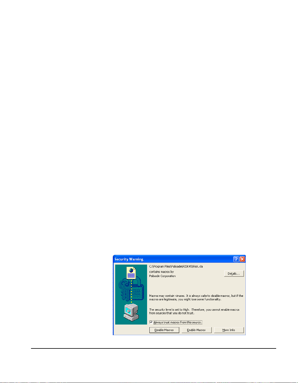
Macro Security Warning Message on Startup
Microsoft Office provides several security settings (under
Tools>Macro>Security) to keep unwanted or malicious macros from
being run in Office applications. A warning message appears each
time you attempt to load a file with macros, unless you use the lowest
security setting. To keep this message from appearing every time you
run a Palisade add-in, Palisade digitally signs their add-in files. Thus,
once you have specified Palisade Corporation as a trusted source,
you can open any Palisade add-in without warning messages. To do
this:
• Click Always trust macros from this source when a Security
Warning dialog (such as the one below) is displayed when
starting Evolver.
Chapter 1: Introduction 9
Page 16

Other Evolver Information
Additional information on Evolver can be found in the following
sources:
Evolver Readme
Evolver Tutorial
This file contains a quick summary of Evolver, as well as any latebreaking news or information on the latest version of your software.
View the Readme file by selecting the Windows Start Menu/
Programs/ Palisade DecisionTools/ Readmes and clicking on Evolver
5.0 – Readme. It is a good idea to read this file before using Evolver.
The Evolver on-line tutorial provides first-time users with a quick
introduction of Evolver and genetic algorithms. The presentation
takes only a few minutes to view. See the Learning Evolver section
below for information on how to access the tutorial.
Learning Evolver
The quickest way to become familiar with Evolver is by using the online Evolver Tutorial, where experts guide you through sample
models in movie format. This tutorial is a multi-media presentation
on the main features of Evolver.
The tutorial can be run by selecting the Evolver Help menu Getting
Started Tutorial command.
10 Installation Instructions
Page 17

Chapter 2: Background
What Is Evolver?...............................................................................13
How does Evolver work?......................................................................14
Genetic Algorithms..................................................................14
What Is Optimization? ..........................................................................15
Why Build Excel Models?.....................................................................16
Why Use Evolver? ..................................................................................16
No More Guessing ...................................................................16
More Accurate, More Meaningful.........................................17
More Flexible.............................................................................17
More Powerful ..........................................................................17
Easier to Use ..............................................................................18
Cost Effective.............................................................................18
Chapter 2: Background 11
Page 18

Chapter 2: Background 12
Page 19
What Is Evolver?
The Evolver software package provides users with an easy way to
find optimal solutions to virtually any type of problem. Simply put,
Evolver finds the best inputs that produce a desired output. You can
use Evolver to find the right mix, order, or grouping of variables that
produces the highest profits, the lowest risk, or the most goods from
the least amount of materials. Evolver is most often used as an add-in
to the Microsoft Excel spreadsheet program; users set up a model of
their problem in Excel, then call up Evolver to solve it.
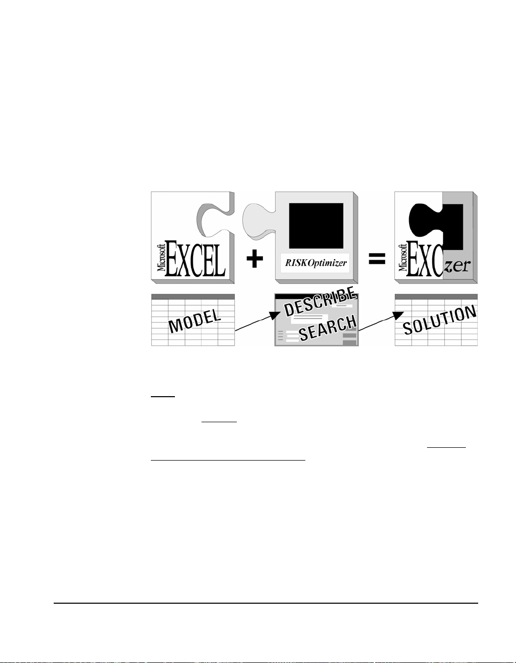
You must first model your problem in Excel, then describe it to the Evolver add-in.
Excel provides all of the formulas, functions, graphs, and macro
capabilities that most users need to create realistic models of their
problems. Evolver
in your model and what you are looking for, and provides the engines
that will find it. Together, they can find optimal solutions to virtually
any problem that can be modeled.
Chapter 2: Background 13
provides the interface to describe the uncertainty
Page 20

How does Evolver work?
Evolver uses a proprietary set of genetic algorithms to search for
optimum solutions to a problem, along with probability distributions
and simulation to handle the uncertainty present in your model.
Genetic Algorithms
Genetic algorithms are used in Evolver to find the best solution for
your model. Genetic algorithms mimic Darwinian principles of
natural selection by creating an environment where hundreds of
possible solutions to a problem can compete with one another, and
only the “fittest” survive. Just as in biological evolution, each solution
can pass along its good “genes” through “offspring” solutions so that
the entire population of solutions will continue to evolve better
solutions.
As you may already realize, the terminology used when working with
genetic algorithms is often similar to that of its inspiration. We talk
about how “crossover” functions help focus the search for solutions,
“mutation” rates help diversify the “gene pool”, and we evaluate the
entire “population” of solutions or “organisms”. To learn more about
how Evolver’s genetic algorithm works, see Chapter 7 - Genetic
Algorithms.
14 What Is Evolver?
Page 21
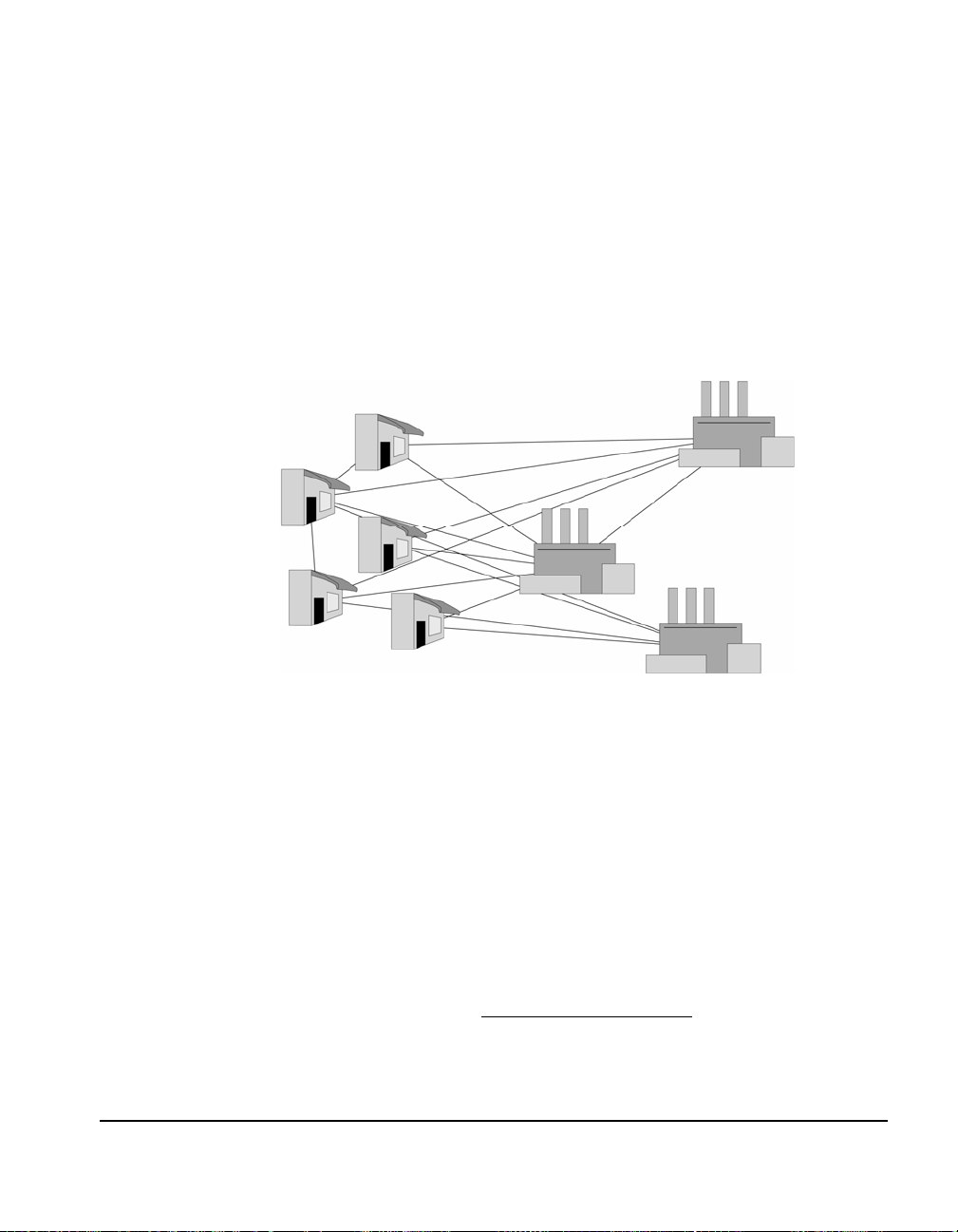
What Is Optimization?
Optimization is the process of trying to find the best solution to a
problem that may have many possible solutions. Most problems
involve many variables that interact based on given formulas and
constraints. For example, a company may have three manufacturing
plants, each manufacturing different quantities of different goods.
Given the cost for each plant to produce each good, the costs for each
plant to ship to each store, and the limitations of each plant, what is
the optimal way to adequately meet the demand of local retail stores
while minimizing the transportation costs? This is the sort of question
that optimization tools are designed to answer.
Optimization often deals with searching for the
combination that yields the most from given resources.
In the example above, each proposed solution would consist of a
complete list of what goods made by what manufacturing plant get
shipped in what truck to what retail store. Other examples of
optimization problems include finding out how to produce the
highest profit, the lowest cost, the most lives saved, the least noise in a
circuit, the shortest route between a set of cities, or the most effective
mix of advertising media purchases. An important subset of
optimization problems involves scheduling, where the goals may
include maximizing efficiency during a work shift or minimizing
schedule conflicts of groups meeting at different times. To learn more
about optimization, see Chapter 6 - Optimization
Chapter 2: Background 15
.
Page 22

Why Build Excel Models?
To increase the efficiency of any system, we must first understand
how it behaves. This is why we construct a working model of the
system. Models are necessary abstractions when studying complex
systems, yet in order for the results to be applicable to the “realworld,” the model must not oversimplify the cause-and-effect
relationships between variables. Better software and increasingly
powerful computers allow economists to build more realistic models
of the economy, scientists to improve predictions of chemical
reactions, and business people to increase the sensitivity of their
corporate models.
In the last few years computer hardware and software programs such
as Microsoft Excel, have advanced so dramatically that virtually
anyone with a personal computer can create realistic models of
complex systems. Excel’s built-in functions, macro capabilities and
clean, intuitive interface allow beginners to model and analyze
sophisticated problems. To learn more about building a model, see
Chapter 9 - Evolver Extras
.
Why Use Evolver?
Evolver’s unique technology allows anyone with a PC and Excel for
Windows to enjoy the benefits of optimization. Before Evolver, those
who wished to increase efficiency or search for optimum solutions
had three choices: guess, use low-powered problem-solving software,
or hire experts in the optimization consulting field to design and
build customized software. Here are a few of the most important
advantages to using Evolver:
No More Guessing
16 What Is Evolver?
When you are dealing with large numbers of interacting variables,
and you are trying to find the best mix, the right order, the optimum
grouping of those variables, you may be tempted to just take an
“educated guess”. A surprising number of people assume that any
kind of modeling and analysis beyond guessing will require
complicated programming, or confusing statistical or mathematical
algorithms. A good optimized solution might save millions of
dollars, thousands of gallons of scarce fuel, months of wasted time,
etc. Now that powerful desktop computers are increasingly
affordable, and software like Excel and Evolver are readily available,
there is little reason to guess at solutions, or waste valuable time
trying out many scenarios by hand.
Page 23

More Accurate, More Meaningful
More Flexible
Evolver allows you to use the entire range of Excel formulas and even
macros to build more realistic models of any system. When you use
Evolver, you do not have to “compromise” the accuracy of your
model because the algorithm you are using can not handle real world
complexities. Traditional “baby” solvers (statistical and linear
programming tools) force the user to make assumptions about the
way the variables in their problem interact, thereby forcing users to
build over-simplified, unrealistic models of their problem. By the
time the user has simplified a system enough that these solvers can be
used, the resulting solution is often too abstract to be practical. Any
problems involving large amounts of variables, non-linear functions,
lookup tables, if-then statements, database queries, or stochastic
(random) elements cannot be solved by these methods, no matter how
simply you try to design your model.
There are many solving algorithms which do a good job at solving
small, simple linear and non-linear types of problems, including hillclimbing, baby-solvers, and other mathematical methods. Even when
offered as spreadsheet add-ins, these general-purpose optimization
tools can only perform numerical optimization. For larger or more
complex problems, you may be able to write specific, customized
algorithms to get good results, but this may require a lot of research
and development. Even then, the resulting program would require
modification each time your model changed.
Not only can Evolver handle numerical problems, it is the only
commercial program in the world that can solve most combinatorial
problems. These are problems where the variables must be shuffled
around (permuted) or combined with each other. For example,
choosing the batting order for a baseball team is a combinatorial
problem; it is a question of swapping players’ positions in the lineup.
Complex scheduling problems are also combinatorial. The same
Evolver can solve all these types of problems, and many more that
nothing else can solve. Evolver’s unique genetic algorithm technology
allows it to optimize virtually any type of model; any size and any
complexity.
More Powerful
Evolver finds better solutions. Most software derives optimum
solutions mathematically and systematically. Too often these
methods are limited to taking an existing solution and searching for
the closest answer that is better. This “local” solution may be far from
the optimal solution. Evolver intelligently samples the entire realm of
possibilities, resulting in a much better “global” solution.
Chapter 2: Background 17
Page 24

Easier to Use
Cost Effective
In spite of its obvious power and flexibility advantages, Evolver
remains easy to use because an understanding of the complex genetic
algorithm techniques it uses is completely unnecessary. Evolver
doesn’t care about the “nuts and bolts” of your problem; it just needs
a spreadsheet model that can evaluate how good different scenarios
are. Just select the spreadsheet cells that contain the variables and tell
Evolver what you are looking for. Evolver intelligently hides the
difficult technology, automating the “what-if” process of analyzing a
problem.
Although there have been many commercial programs developed for
mathematical programming and model-building, spreadsheets are by
far the most popular, with literally millions being sold each month.
With their intuitive row and column format, spreadsheets are easier
to set up and maintain than other dedicated packages. They are also
more compatible with other programs such as word processors and
databases, and offer more built-in formulas, formatting options,
graphing, and macro capabilities than any of the stand-alone
packages. Because Evolver is an add-in to Microsoft Excel, users have
access to the entire range of functions and development tools to easily
build more realistic models of their system.
Many companies have hired trained consultants to provide
customized optimization systems. Such systems will often perform
quite well, but may require many months and a large investment to
develop and implement. These systems are also difficult to learn, and
therefore require costly training and constant maintenance. If your
system must be altered, you may need to develop a whole new
algorithm to find optimal solutions. For a considerably smaller
investment, Evolver supplies the most powerful genetic algorithms
available and allows for quick and accurate solutions to a wide
variety of problems. Because it works in an intuitive and familiar
environment, there is virtually no costly training and maintenance.
You may even wish to add Evolver’s optimization power to your own
custom programs. In just a few days, you could use Visual Basic to
develop your own scheduling, distribution, manufacturing or
financial management system. See the Evolver Developer Kit for
details on developing an Evolver-based application.
18 What Is Evolver?
Page 25

Chapter 3: Evolver: Step-by-Step
Introduction.......................................................................................21
The Evolver Tour ..............................................................................23
Starting Evolver......................................................................................23
The Evolver Toolbar.................................................................23
Opening an Example Model...................................................23
The Evolver Model Dialog ...................................................................24
Selecting the Target Cell.......................................................................25
Adding Adjustable Cell Ranges..........................................................25
Selecting a Solving Method....................................................27
Constraints ..............................................................................................28
Adding a Constraint.................................................................29
Simple Range of Values and Formula Constraints............29
Other Evolver Options ..........................................................................32
Stopping Conditions................................................................32
View Options ............................................................................34
Running the Optimization...................................................................35
The Evolver Watcher................................................................36
Stopping the Optimization.....................................................37
Summary Report.......................................................................38
Placing the Results in Your Model........................................39
Chapter 3: Evolver: Step-by-Step 19
Page 26

20
Page 27

Introduction
In this chapter, we will take you through an entire Evolver
optimization one step at a time. If you do not have Evolver installed
on your hard drive, please refer to the installation section of Chapter
1: Introduction and install Evolver before you begin this tutorial.
We will start by opening a pre-made spreadsheet model, and then we
will define the problem to Evolver using probability distributions and
the Evolver dialogs. Finally we will oversee Evolver’s progress as it is
searching for solutions, and explore some of the many options in the
Evolver Watcher. For additional information about any specific topic,
see the index at the back of this manual, or refer to Chapter 5: Evolver
Reference.
NOTE: The screens shown below are from Excel 2007. If you are using
other versions of Excel, your windows may appear slightly different
from the pictures.
The problem-solving process begins with a model that accurately
represents your problem. Your model must be able to evaluate a
given set of input values (adjustable cells) and produce a numerical
rating of how well those inputs solve the problem (the evaluation or
“fitness” function). As Evolver searches for solutions, this fitness
function provides feedback, telling Evolver how good or bad each
guess is, thereby allowing Evolver to breed increasingly better
guesses. When you create a model of your problem you must pay
close attention to the fitness function, because Evolver will be doing
everything it can to maximize (or minimize) this cell.
Chapter 3: Evolver: Step-by-Step 21
Page 28

22 Introduction
Page 29
The Evolver Tour
Starting Evolver
To start Evolver, either: 1) click the Evolver icon in your Windows
desktop, or 2) select Palisade DecisionTools then Evolver 5.0 in the
Windows Start menu Programs entries. Each of these methods starts
both Microsoft Excel and Evolver.
The Evolver Toolbar
Opening an Example Model
When Evolver is loaded, a new Evolver ribbon or toolbar is visible in
Excel. This toolbar contains buttons which can be used to specify
Evolver settings and start, pause, and stop optimizations.
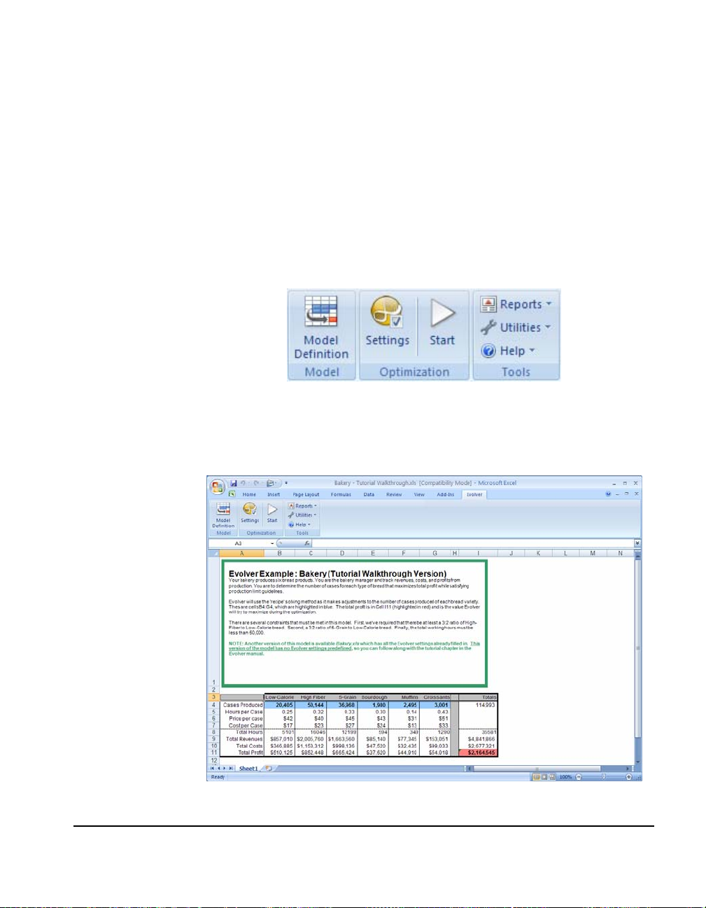
To review the features of Evolver, you'll examine an example model
that was installed when you installed Evolver. To do this:
1) Open the Bakery–TutorialWalkthrough.XLS worksheet using
the Help menu Example Spreadsheets command.
Chapter 3: Evolver: Step-by-Step 23
Page 30
This example sheet contains a simple profit maximization problem for
a bakery business. Your bakery produces 6 bread products. You are
the bakery manager and track revenues, costs, and profits from
production. You are to determine the number of cases for each type
of bread that maximizes total profit while satisfying production limit
guidelines. The guidelines you face include 1) meeting the production
quota for low calorie bread, 2) maintaining an acceptable ratio of high fiber
to low calorie, 3) maintaining an acceptable ratio of 5 grain to low calorie,
and 4) keeping production time within limits for person hours used.
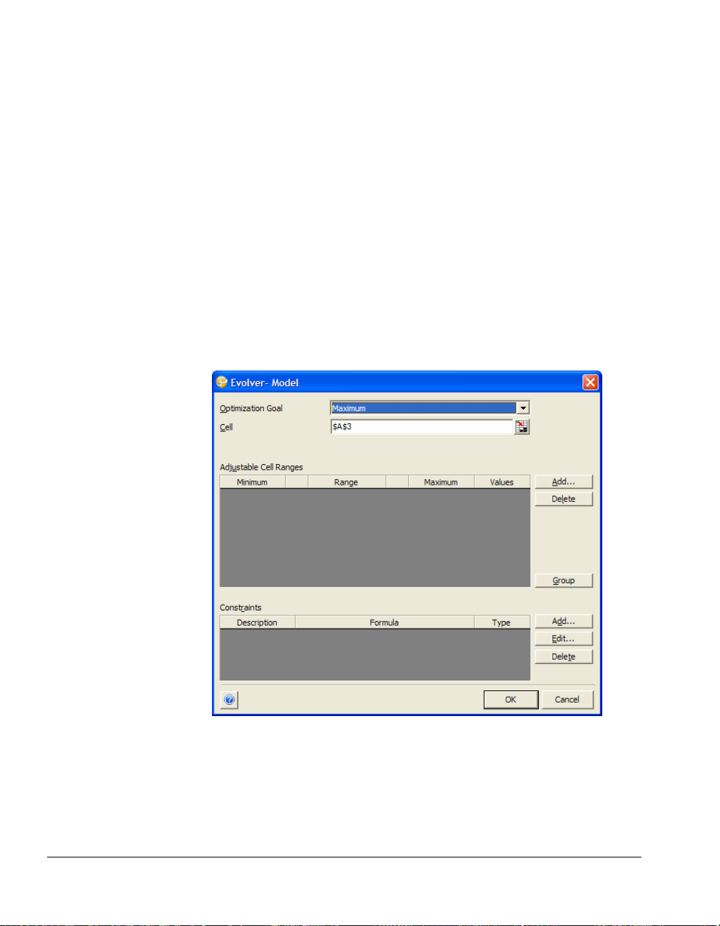
The Evolver Model Dialog
To set the Evolver options for this worksheet:
1) Click the Evolver Model icon on the Evolver toolbar (the one on
the far left).
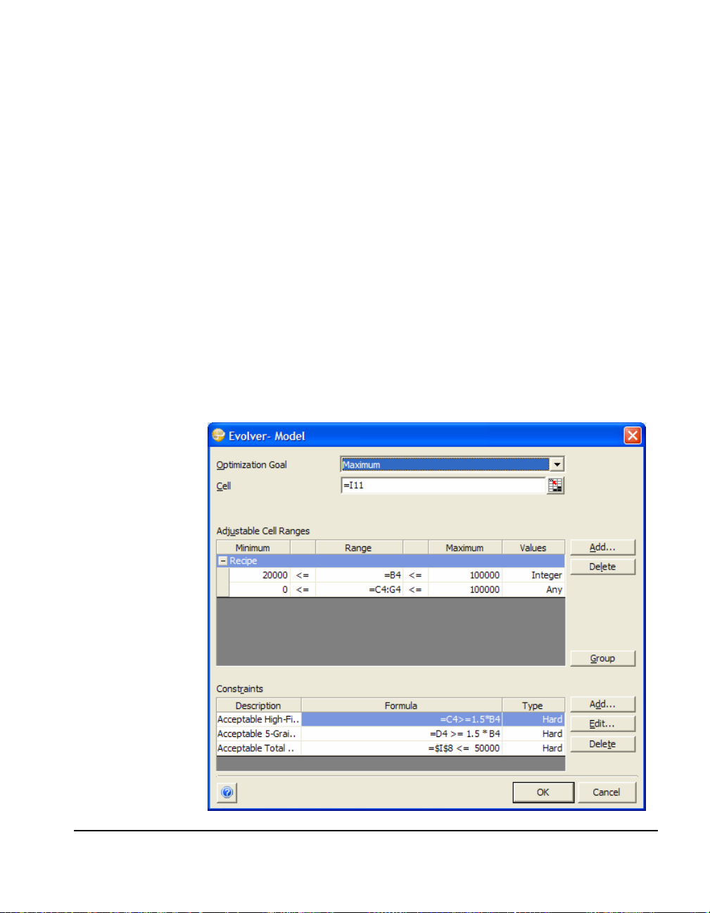
This displays the following Evolver Model dialog box:
The Evolver Model Dialog is designed so users can describe their
problem in a simple, straightforward way. In our tutorial example, we
are trying to find the number of cases to produce for the different
bread products in order to maximize overall total profit.
24 The Evolver Tour
Page 31

Selecting the Target Cell
The "total profit" in the example model is what's known as the target
cell. This is the cell whose value you are trying to minimize or
maximize, or the cell whose value you are trying to make as close as
possible to a pre-set value. To specify the target cell:
1) Set the “Optimization Goal” option to “Maximum.”
2) Enter the target cell, $I$11, in the “Cell” field.
Cell references can be entered in Evolver dialog fields two ways: 1)
You may click in the field with your cursor, and type the reference
directly into the field, or 2) with your cursor in the selected field, you
may click on Reference Entry icon to select the worksheet cell(s)
directly with the mouse.
Adding Adjustable Cell Ranges
Now you must specify the location of the cells that contain values
which Evolver can adjust to search for solutions. These variables are
added and edited one block at a time through the Adjustable Cells
Ranges section of the Model Dialog. The number of cells you can enter
in Adjustable Cells Ranges depends on the version of Evolver you are
using.
1) Click the “Add” button in the "Adjustable Cell Ranges" section.
2) Select $C$4:$G$4 as the cells in Excel you want to add as an
adjustable cell range.
Entering the
Min-Max Range
for Adjustable
Cells
Chapter 3: Evolver: Step-by-Step 25
Most of the time you'll want to restrict the possible values for an
adjustable cell range to a specific minimum-maximum range. In
Evolver this is known as a "range" constraint. You can quickly enter
this min-max range when you select the set of cells to be adjusted.
For the Bakery example, the minimum possible value for cases
produced for each of the bread products in this range is 0 and the
maximum is 100,000. To enter this range constraint:
1) Enter 0 in the Minimum cell and 100,000 in the Maximum cell.
2) In the Values cell, select Integer from the drop-down list
Page 32

Now, enter a second cell range to be adjusted:
1) Click Add to enter a second adjustable cell.
2) Select cell B4.
3) Enter 20,000 as the Minimum and 100,000 as the Maximum.
26 The Evolver Tour
Page 33
This specifies the last adjustable cell, B4, representing the production
level for low calorie bread.
If there were additional variables in this problem, we would continue
to add sets of adjustable cells. In Evolver, you may create an
unlimited number of groups of adjustable cells. To add more cells,
click the “Add” button once again.
Later, you may want to check the adjustable cells or change some of
their settings. To do this, simply edit the min-max range in the table.
You may also select a set of cells and delete it by clicking the “Delete”
button.
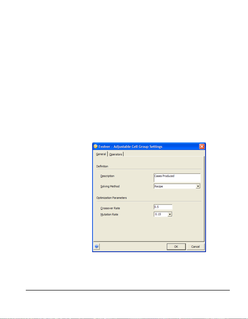
Selecting a Solving Method
When defining adjustable cells, you can specify a solving method to be
used. Different types of adjustable cells are handled by different
solving methods. Solving methods are set for a Group of adjustable
cells and are changed by clicking the “Group” button and displaying
the Adjustable Cell Group Settings dialog box. Often you'll use the
default “recipe” solving method where each cell’s value can be
changed independently of the others. Since this is selected as the
default method, you don't have to change it.
The “recipe” and “order” solving methods are the most popular and
they can be used together to solve complex combinatorial problems.
Specifically, the “recipe” solving method treats each variable as an
ingredient in a recipe, trying to find the “best mix” by changing each
variable’s value independently. In contrast, the “order” solving
Chapter 3: Evolver: Step-by-Step 27
Page 34

method swaps values between variables, shuffling the original values
to find the “best order.”
For this model, leave the Solving Method as Recipe and simply:
♦ Enter the label "Cases Produced" in the Description field.
Constraints
Evolver allows you to enter constraints which are conditions that
must be met for a solution to be valid. In this example model there
are three additional constraints that must be met for a possible set of
production levels for each of the bread products to be valid. These
are in addition to the range constraints we already entered for the
adjustable cells. They are:
1) Maintaining an acceptable ratio of high fiber to low calorie
bread (high fiber cases produced >= 1.5 * low calorie cases
produced)
2) Maintaining an acceptable ratio of 5 grain to low calorie bread
(5 grain cases produced >= 1.5 * low calorie cases produced)
3) Keeping production time within limits for person hours used
(total person hours used < 50,000)
Each time Evolver generates a possible solution to your model it
checks that the constraints you have entered are valid.
Constraints are displayed in the bottom Constraints section of the
Evolver Model dialog box. Two types of constraints can be specified
in Evolver:
♦ Hard. These are conditions that must be met for a solution to be
valid (i.e., a hard iteration constraint could be C10<=A4; in this
case, if a solution generates a value for C10 that is greater than the
value of cell A4, the solution will be thrown out)
♦ Soft. These are conditions which we would like to be met as
much as possible, but which we may be willing to compromise
for a big improvement in fitness or target cell result. (i.e., a soft
constraint could be C10<100. In this case, C10 could go over 100,
but when that happens the calculated value for the target cell
would be decreased according to the penalty function you have
entered).
28 The Evolver Tour
Page 35
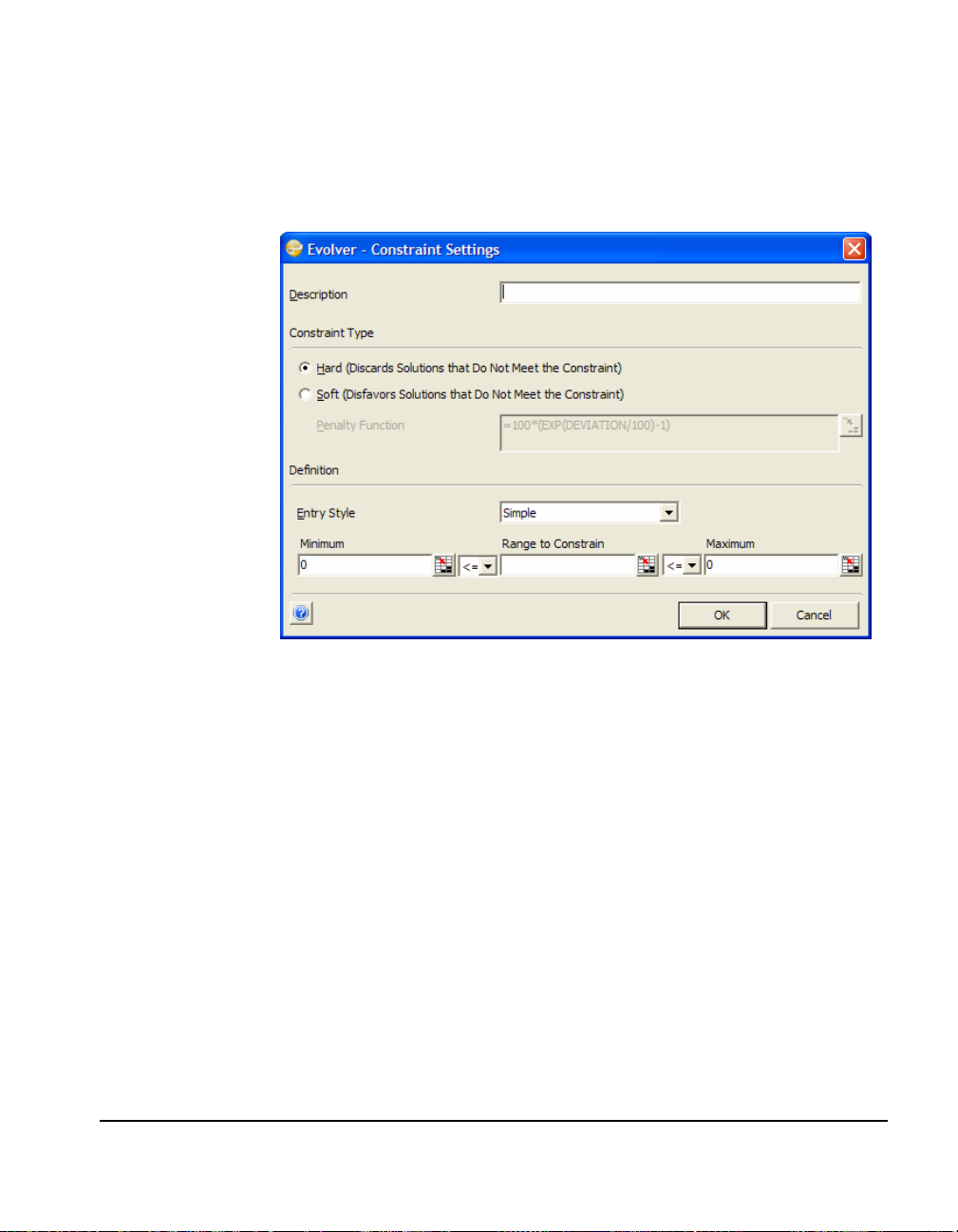
Adding a Constraint
To add a constraint:
1) Click the Add button in the Constraints section of the main
Evolver dialog.
This displays the Constraint Settings dialog box, where you enter the
constraints for your model.
Simple Range of Values and Formula Constraints
Two formats – Simple and Formula – can be used for entering
constraints. The Simple Range of Values format allows constraints to
be entered using simple <,<=, >, >= or = relations. A typical Simple
Range of Values constraint would be 0<Value of A1<10, where A1 is
entered in the Cell Range box, 0 is entered in the Min box and 10 is
entered in the Max box. The operator desired is selected from the
drop down list boxes. With a Simple Range of Values format
constraint, you can enter just a Min value, just a Max or both.
A formula constraint, on the other hand, allows you to enter any valid
Excel formula as a constraint, such as A19<(1.2*E7)+E8. For each
possible solution Evolver will check whether the entered formula
evaluates to TRUE or FALSE to see if the constraint has been met. If
you want to use a boolean formula in a worksheet cell as a constraint,
simply reference that cell in the Formula field of the Constraint
Settings dialog box.
Chapter 3: Evolver: Step-by-Step 29
Page 36
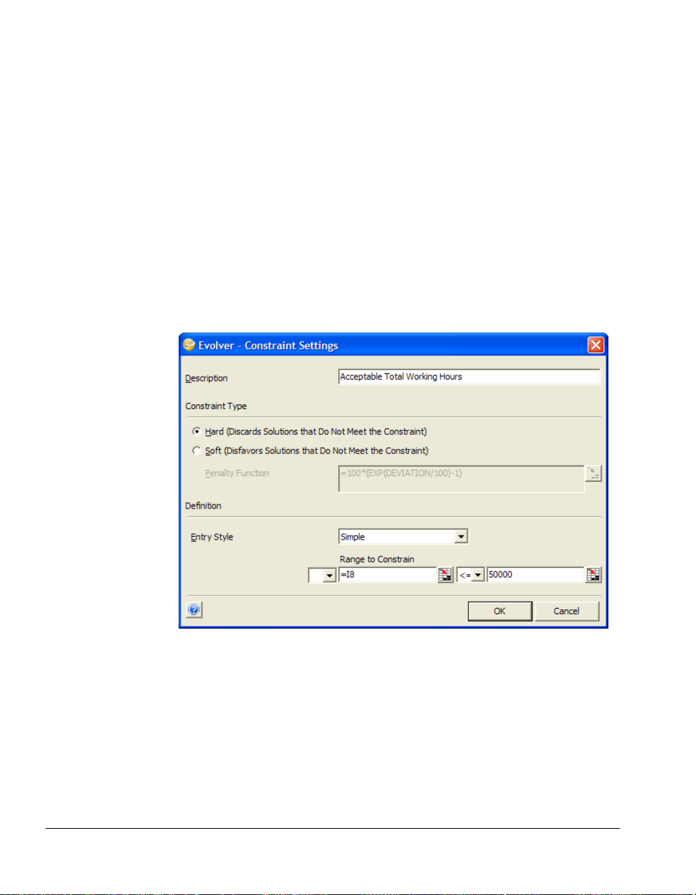
To enter the constraints for the Bakery model you'll specify three new
hard constraints. These are hard constraints as the entered conditions
must be met or the possible solution will be discarded by Evolver.
First, enter the Simple Range of Values format hard constraints:
1) Enter " Acceptable Total Working Hours" in the description box.
2) In the Range to Constrain box, enter I8.
3) Select the <= operator to the right of the Range to Constrain.
4) Enter 50,000 in the Maximum box.
5) Clear the default value of 0 in the Minimum box.
6) To the left of Range to Constrain, clear the operator by selecting
a blank from the drop down list
7) Click OK to enter this constraint.
30 The Evolver Tour
Page 37
Now, enter the formula format hard constraints:
1) Click Add to display the Constraint Settings dialog box again.
2) Enter "Acceptable ratio of high fiber to low calorie" in the
description box.
3) In the Entry Style box, select Formula.
4) In the Constraint Formula box, enter C4>= 1.5*B4.
5) Click OK.
6) Click Add to display the Constraint Settings dialog box again.
7) Enter "Acceptable ratio of 5-grain to low calorie" in the
description box.
8) In the Entry Style box, select Formula.
9) In the Constraint Formula box, enter D4>= 1.5*B4.
10) Click OK
Your Model dialog with the completed constraints section should
look like this.
Chapter 3: Evolver: Step-by-Step 31
Page 38
Other Evolver Options
Options such as Update the Display, Random Number Seed and Stopping
Conditions are available to control how Evolver operates during an
optimization. Let's specify some stopping conditions and display
update settings.
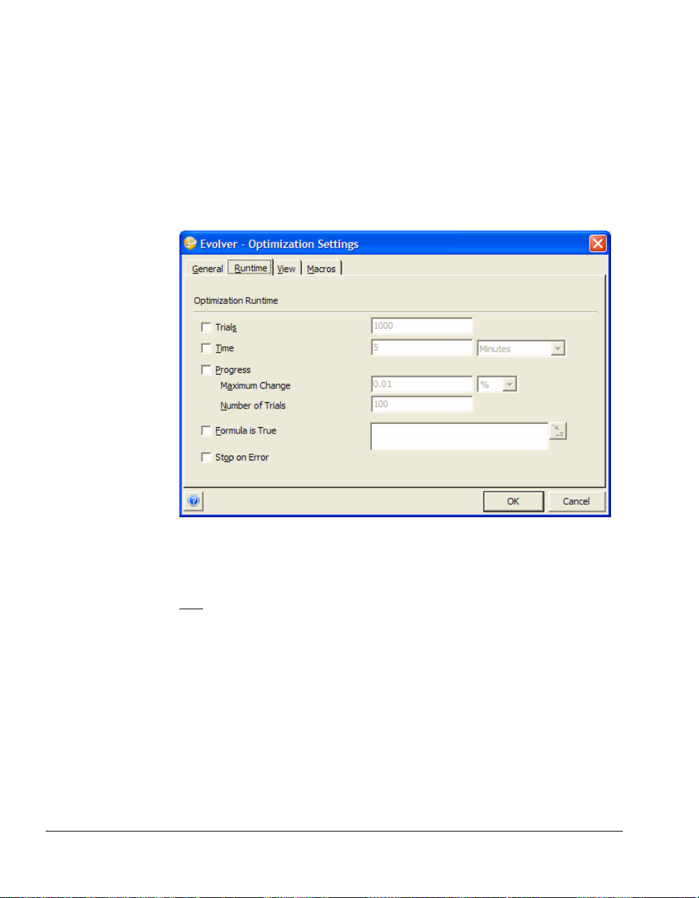
Stopping Conditions
Evolver will run as long as you wish. The stopping conditions allow
Evolver to automatically stop when either: a) a certain number of
scenarios or “trials” have been examined, b) a certain amount of time has
elapsed, c) no improvement has been found in the last
entered Excel formula evaluates to TRUE. To view and edit the stopping
conditions:
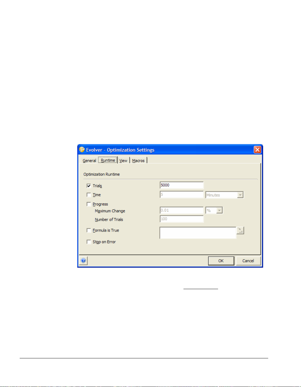
1) Click the Optimization Settings icon on the Evolver toolbar.
2) Select the Runtime tab.
n scenarios or d) the
In the Optimization Settings dialog you can select any combination of
these optimization stopping conditions, or none at all
more than one stopping condition, Evolver will stop when any one of
the selected conditions are met. If you do not select any stopping
conditions, Evolver will run forever, until you stop it manually by
pressing the “stop” button in the Evolver toolbar.
32 The Evolver Tour
. If you select
Page 39

Trials
This option sets the
number of “trials”
that you would like
Evolver to run. In
each trial, Evolver
evaluates one
complete set of
variables or one
possible solution to
the problem.
Evolver will stop
after the specified
amount of time has
elapsed. This
number can be a
fraction (4.25).
Minutes
Change in last
This stopping
condition is the
most popular
because it keeps
track of the
improvement and
allows Evolver to
run until the rate of
improvement has
decreased. For
example, Evolver
could stop if 100
trials have passed
and we still haven’t
had any change in
the best scenario
found so far.
Formula is True
Evolver will stop if
the entered Excel
formula evaluates to
TRUE in a model
recalculation.
♦ Turn off all stopping conditions to let Evolver run freely.
Chapter 3: Evolver: Step-by-Step 33
Page 40
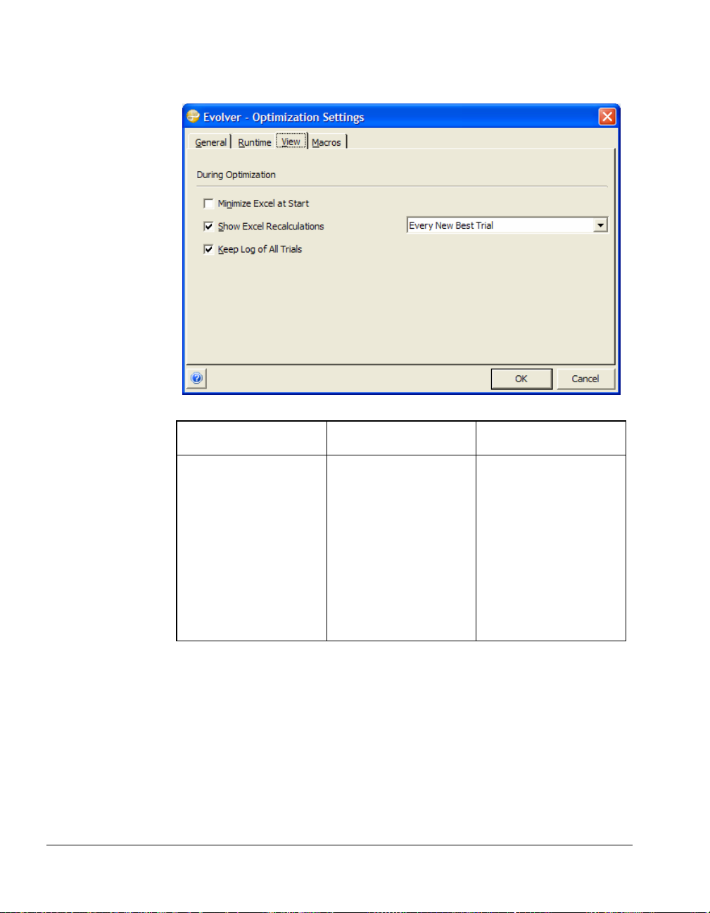
View Options
While Evolver runs, a set of options are available on the View Tab to
determine what you will see on-screen.
The During Optimization options include:
Every Trial
This option redraws the
screen after each
calculation, allowing you to
see Evolver adjusting the
variables and calculating
the output. We suggest
this option be turned on
while you are learning
Evolver, and also each time
you use Evolver on a new
model, to verify that your
model is calculating
correctly.
Every New Best Trial
This option redraws the
screen each time Evolver
generates a new best
answer, allowing you to
see the current optimal
solution at any time during
the optimization.
This option never redraws
the screen during the
optimization. This results
in the fastest possible
optimizations but provides
little feedback on
calculated results during
the run.
Never
♦ Turn on the “Every Trial”
34 The Evolver Tour
Page 41

Running the Optimization
Now, all that remains is to optimize this model to maximize total
profit while satisfying production limit guidelines. To do this:
1) Click OK to exit the Optimization Settings dialog.
2) Click the Start Optimization icon
As Evolver begins working on your problem, you will see the current
best values for your adjustable cells – Cases Produced - in your
spreadsheet. The best value for Total Profit is shown in the
highlighted cell.
During the run, the Progress window displays: 1) the best solution
found so far, 2) the original value for the target cell when the Evolver
optimization began, 3) the number of trials of your model that have
been executed and number of those trials which were valid; i.e., all
constraints were met and 4) the time that has elapsed in the
optimization.
Any time during the run you can click the Excel Updating Options
icon to see a live updating of the screen each trial.
Chapter 3: Evolver: Step-by-Step 35
Page 42

The Evolver Watcher
Evolver can also display a running log of the simulations performed
for each trial solution. This is displayed in the Evolver Watcher while
Evolver is running. The Evolver Watcher allows you to explore and
modify many aspects of your problem as it runs. To view a running
log of the simulations performed:
1) Click the Watcher (magnifying glass) icon in the Progress
window to display the Evolver Watcher
2) Click the Log tab.
In this report the results of the simulation run for each trial solution is
shown. The column for Result shows by trial the value of the target
cell that you are trying to maximize or minimize - in this case, the
Total Profit in $I$11. The columns for C4 through G4 identify the
values used for your adjustable cells.
36 The Evolver Tour
Page 43

Stopping the Optimization
After five minutes, Evolver will stop the optimization. You can also
stop the optimization by:
1) Clicking the Stop icon in the Evolver Watcher or Progress
windows.
When the Evolver process stops, Evolver displays the Stopping
Options tab which offers the following choices:
These same options will automatically appear when any of the
stopping conditions that were set in the Evolver Optimization
Settings dialog are met.
Chapter 3: Evolver: Step-by-Step 37
Page 44

Summary Report
Evolver can create an optimization summary report that contains
information such as date and time of the run, the optimization
settings used, the value calculated for the target cell and the value for
each of the adjustable cells.
This report is useful for comparing the results of successive
optimizations.
38 The Evolver Tour
Page 45

Placing the Results in Your Model
To place the new, optimized mix of production levels for the bakery
to each of the six types of bread in your worksheet:
1) Click on the “Stop” button.
2) Make sure the "Update Adjustable Cell Values Shown in
Workbook to" option is set to “Best”
You will be returned to the BAKERY – TUTORIAL
WALKTHROUGH.XLS spreadsheet, with all of the new variable
values that created the best solution.
IMPORTANT NOTE: Although in our example you can see that
Evolver found a solution which yielded a total profit of 3,940,486,
your result may be higher or lower than this. These differences are
due to an important distinction between Evolver and all other
problem-solving algorithms: it is the random nature of Evolver’s
genetic algorithm engine that enables it to solve a wider variety of
problems, and find better solutions.
Chapter 3: Evolver: Step-by-Step 39
Page 46

When you save any sheet after Evolver has run on it (even if you
“restore” the original values of your sheet after running Evolver), all
of the Evolver settings in the Evolver dialogs will be saved along with
that sheet. The next time that sheet is opened, all of the most recent
Evolver settings load up automatically. All of the other example
worksheets have the Evolver settings pre-filled out and ready to be
optimized.
NOTE: If you want to take a look at the Bakery model with all
optimization settings pre-filled out, open the example model
Bakery.XLS
40 The Evolver Tour
Page 47

Chapter 4: Example Applications
Introduction.......................................................................................43
Advertising Selection.......................................................................45
Alphabetize........................................................................................47
Assignment of Tasks........................................................................49
Bakery................................................................................................51
Budget Allocation.............................................................................53
Chemical Equilibrium.......................................................................55
Class Scheduler................................................................................57
Code Segmenter...............................................................................59
Dakota: Routing With Constraints..................................................63
Job Shop Scheduling.......................................................................65
Radio Tower Location......................................................................67
Portfolio Balancing...........................................................................69
Portfolio Mix......................................................................................71
Power Stations..................................................................................73
Purchasing ........................................................................................75
Chapter 4: Example Applications 41
Page 48

Salesman Problem...........................................................................77
Space Navigator............................................................................... 79
Trader ................................................................................................ 81
Transformer......................................................................................83
Transportation..................................................................................85
42
Page 49

Introduction
This chapter explains how Evolver can be used in a variety of
applications. These example applications may not include all of the
features you would want in your own models, and are most effective
as idea generators and templates. All examples illustrate how
Evolver finds solutions by relying on the relationships that already
exist in your worksheet, so it is important that your worksheet model
accurately portray the problem you are trying to solve.
All Excel worksheet examples can be found within your EVOLVE32
directory, in a sub-directory called “EXAMPLES". They are listed
alphabetically in this chapter. Examples use the following colorcoding conventions:
♦
blue outlined cells. . . . . . adjustable cells that Evolver will
be adjusting.
♦
red outlined cells .. . . . . . the target or goal cell.
Each example comes with all Evolver settings pre-selected, including
the target cell, adjustable cells, solving methods and constraints. You
are encouraged to examine these dialog settings before optimizing.
By studying the formulas and experimenting with different Evolver
settings, you can get a better understanding of how Evolver is used.
The models also let you replace the sample data with your own
“user” data. If you decide to modify or adapt these example sheets,
you may wish to save them with a new name to preserve the original
examples for reference.
Chapter 4: Example Applications 43
Page 50

44 Introduction
Page 51
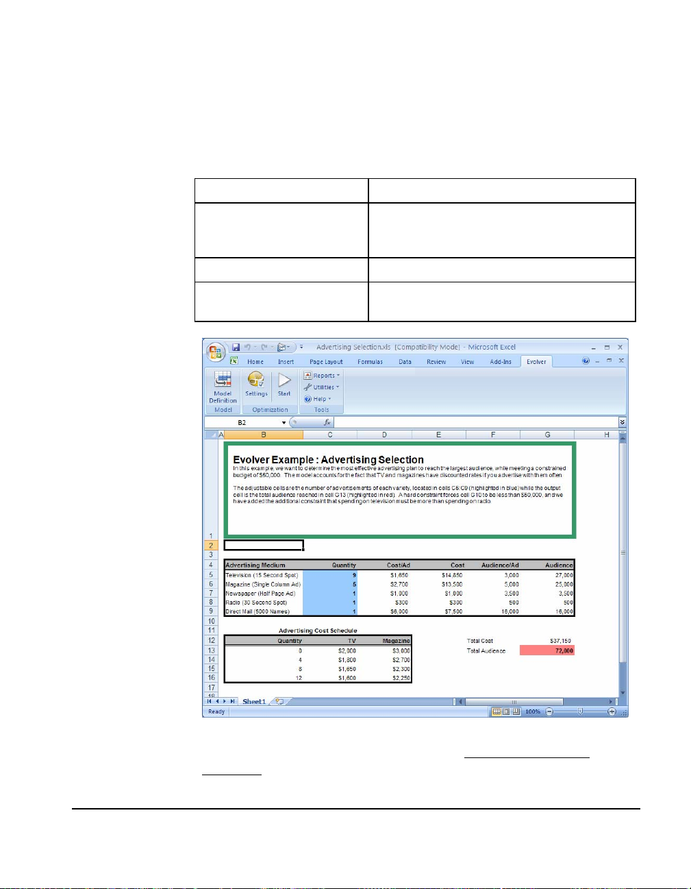
Advertising Selection
An ad agency must figure out the most efficient way to spend its
advertising dollars to maximize the coverage for its target audience.
It must not spend over its budget, and the amount spent on TV must
be more than the amount spent on radio.
Example file:
Goal:
Solving method:
Similar problems:
Advertising Selection.xls
Allocate advertising purchases, within your
budget, among media which have various
price breaks. Maximize people reached.
budget
budget-type problems with additional
constraints.
How The Model
Works
The first thing we need to do is choose a solving method that tells
Evolver what to do with the variables. See Chapter 5: Complete
Reference for descriptions of the different solving methods.
Chapter 4: Example Applications 45
Page 52

This is basically a budget-type problem with the additional constraint
that TV spending must be more than radio spending.
How To Solve It
The variables to be adjusted by Evolver are in cells C5:C9. We will
ask Evolver to juggle them using the “budget” method, to allow each
variable to be an independent value. The total audience is calculated
with the SUM function in cell G13; this is the cell we will ask Evolver
to maximize. The hard constraints specify that TV spending must be
more than radio spending.
46 Advertising Selection
Page 53
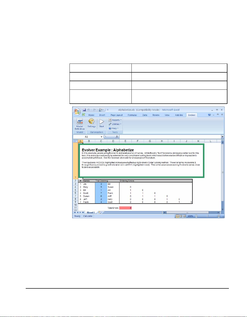
Alphabetize
This is a list of seven names which we would like Evolver to
alphabetize. Although this example is simple, Evolver could handle
complex sorts where data was interdependent, or names were
weighted more heavily based upon other information in the model.
Example file:
Goal:
Solving method:
Similar problems:
Alphabetize.xls
Alphabetize the list of names.
order
Any sorting problem that is beyond the
capability of Excel.
How The Model
Works
The “Alphabetize.xls” file is a very simple model which illustrates
Evolver’s sorting possibilities. Column B contains the first names of
seven people, and column A contains the corresponding “ID””
number for each person. Column D uses the VLOOKUP function in
Excel to translate whatever number is chosen in Column C into its
corresponding name. Cells E4:E9 use a simple penalty function which
assigns a value of 1 each time an earlier name gets listed after a later
name. The sum of all these errors is in cell E11, our target cell.
Chapter 4: Example Applications 47
Page 54
How To Solve It
In this model, the variables to be adjusted are located in column C
(C3:C9). We will ask Evolver to juggle cells C3:C9 using the “order”
solving method. The “order” solving method tells Evolver to
rearrange the order of the selected values, trying different
permutations of those variables rather than trying out new values.
We will ask Evolver to find the value closest to 0 for the total error in
cell E11, because when this target cell hits 0, that means that all the
names are in the correct order.
By not selecting any stopping criteria in the Evolver Options dialog,
you are telling Evolver to keep working forever until it is manually
stopped by clicking the “stop” button on the Evolver toolbar. But in
this model we have selected the “value closest to” option, so Evolver
will
automatically stop if it finds a solution that meets your “value
closest to” value of 0.
We are using a smaller population size because although there are no
fast rules about choosing an optimal population size, generally, we
can select a smaller population size when working with problems that
have a smaller number of total possible solutions, so we focus more
quickly on breeding the top performing solutions. In this problem,
there are only 5040 possible orders of the 7 names.
48 Alphabetize
Page 55

Assignment of Tasks
This example models a common problem involving resource
allocation. In this problem, a manager has 16 workers to perform 16
tasks. Each worker's ability to perform each task has been rated on a
scale of 1 to 10 (1= cannot do the task, 10= perfect at the task). The
challenge here is to match each worker to a task so that the overall
productivity of the workers is maximized.
Example file:
Goal:
Solving method:
Similar problems:
Assignment of Tasks.xls
Assign 16 workers to 16 tasks so the overall
efficiency is maximized.
order
assignment problems, scheduling meetings at
times when the most workers would be
happiest to meet, finding the best machines
for a series of jobs.
Chapter 4: Example Applications 49
Page 56

The model provides a 16 by 16 grid in cells B4:Q19 where each worker
has been rated for each task. The "chosen task" column (column S) to
the right of the grid arbitrarily assigns each worker to one task. The
next column over (column U) checks what task was assigned, and
enters each worker's rating for that task. Finally, the total score of the
entire solution (in cell U21) is the sum of adding up all the individual
ratings.
How The Model
Works
How To Solve It
There is only one person for each task, so no numbers can be
duplicates, and each number must be used once. Each worker’s
rating at that task is recorded in column U using the INDEX()
function. These scores are summed in cell U21 to figure out the total
score for that set of assignments.
Evolver is asked to juggle the “chosen task” variables, located in
column S (S4:S19). We will ask Evolver to juggle these cells using the
“order” solving method. This method will shuffle the existing values
in those cells around, so be sure that there is only one of each value
represented before you begin the optimization. We will ask Evolver
to find the maximum value for cell U21, the target cell, because the
higher this cell gets, the better the overall assignment.
50 Assignment of Tasks
Page 57
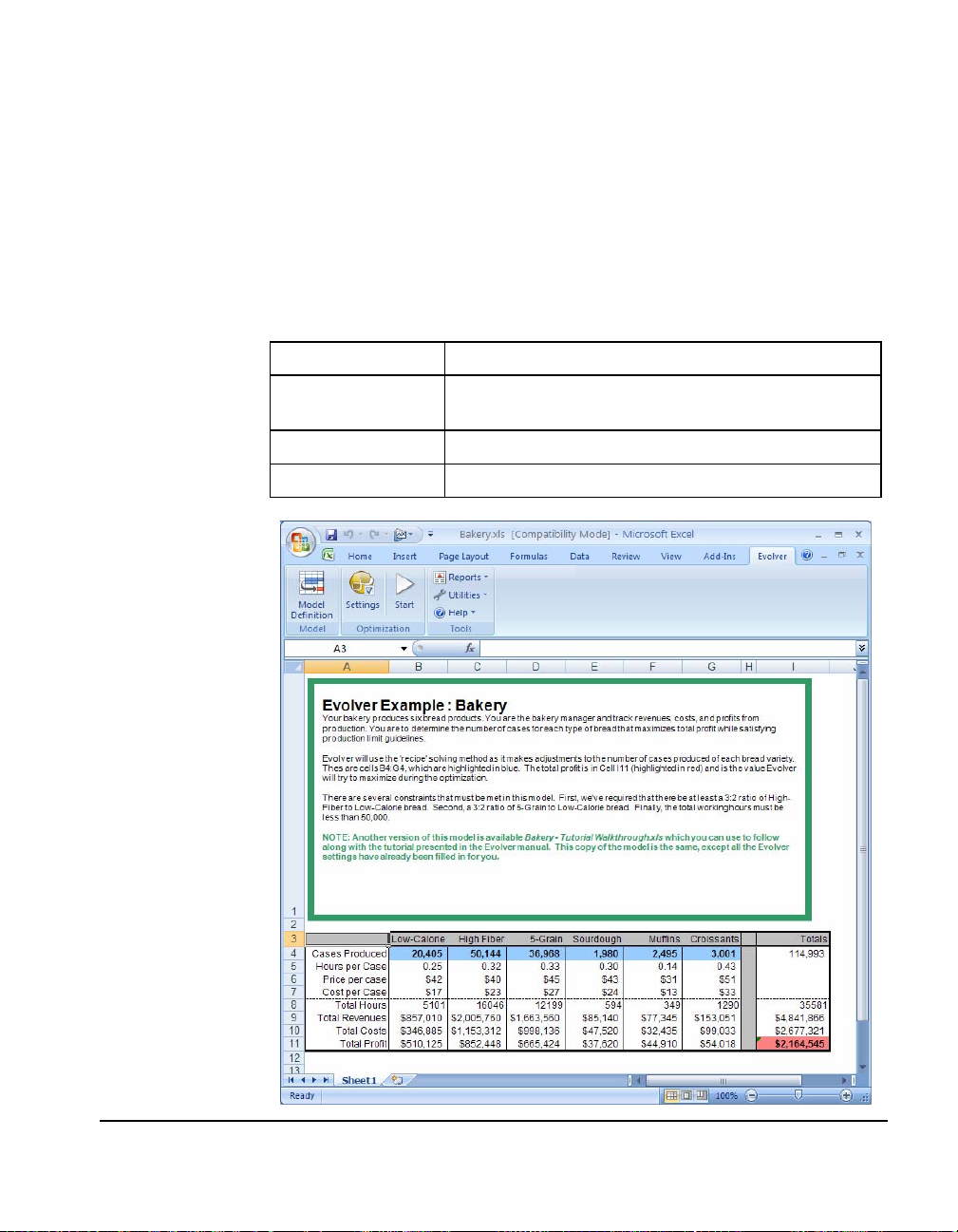
Bakery
This example illustrates a common problem in production decision
problems, where finding the right amount of each product to produce
becomes very difficult... even with only a few items. A bakery owner
must determine the number of cases to produce for each kind of
bread, in order to maximize the total profit of the bakery. Be sure to
also observe the limitations outlined, such as the total number of
employee hours, and the correct ratios of products to be produced.
(Note: this model is covered in detail in Chapter 3: Evolver Step-by-Step)
Example file:
Goal:
Solving method:
Similar problems:
Bakery.xls
Find the optimal amount of each kind of bread to bake
to satisfy all quotas and maximize profits.
recipe
developing portfolios, manufacturing planning
Chapter 4: Example Applications 51
Page 58

How The Model
Works
This problem lists the amount of each bread product to be produced
across the top of the chart in row 4. When we adjust these quantity
variables (B4:G4), the model computes the hours and costs it would
take, as well as the profit that would be generated from baking that
amount. The profit (in cells B11:G11) are added together in cell I11,
which becomes the target cell to maximize.
The model also has three constraints. Each constraint listed is a hard
constraint. One is a Simple Range of Values format constraint and
two are constraints entered as Excel formulas.
How To Solve It
Evolver is asked to find the values for cells B4:G4 (the amounts to
make) that will maximize the value in cell I11 (the total profit). Since
each value it finds can be independent of the others, we will use the
“recipe” solving method. We will also ask Evolver to observe the
constraints for cells C4, D4 and I8.
52 Bakery
Page 59

Budget Allocation
A senior executive wants to find the most effective way to distribute
funds among the various departments of the company to maximize
profit. Below is a model of a business and its projected profit for the
next year. The model estimates next year’s profit by examining the
annual budget and making assumptions about, for example, how
advertising affects sales. This is a simple model, but it illustrates how
you can set up any model and use Evolver to feed inputs into it to
find the best output.
Example file:
Goal:
Solving method:
Similar problems:
Budget Allocation.xls
Allocate the annual budget among five
departments to maximize next year’s profits.
budget
Allocate any scarce resource (such as labor,
money, gas, time) to entities that can use them
in different ways or with different efficiencies.
Chapter 4: Example Applications 53
Page 60

How The Model
Works
The file “Budget Allocation.xls” models the effects of a company’s
budget on its future sales and profit. Cells C4:C8 (the variables)
contain the amounts to be spent on each of the five departments.
These values total the amount in cell C10, the total annual budget for
the company. This budget is set by the company and is
unchangeable.
Cells F6:F10 compute an estimate of the demand for the company’s
product next year, based on the advertising and marketing budgets.
The amount of actual sales is the minimum of the calculated demand
and the supply. The supply is dependent upon the money allocated
to the production and operations departments.
How To Solve It
Maximize the profit in cell I16 by using the “budget” solving method
to adjust the values in cells C4:C8. Set the independent ranges for
each of the adjustable cells for the budget for each department, to
keep Evolver from trying negative numbers, or numbers which would
not make suitable solutions (e.g., all advertising and no production)
for the departmental budget.
The “budget” solving method works like the “recipe” solving
method, in that it is trying to find the right “mix” of the chosen
variables. When you use the budget method, however, you add the
constraint that all variables must sum up to the same number as they
did before Evolver started optimizing.
54 Budget Allocation
Page 61

Chemical Equilibrium
Any process which can be modeled to produce a result given some
initial conditions can be optimized by Evolver. This example shows
how Evolver can find levels of different chemicals (products and
reactants) that minimizes the free energy after a reaction has reached
equilibrium. In complicated chemical processes the ingredients
(reagents) and the products continually re-form into one another until
the concentration of the compounds becomes constant; when
“equilibrium” is reached. At any time after equilibrium is reached, a
steady percentage of the equilibrium chemicals might be reagents
(e.g. 5%), and a steady percentage would be products (95%).
Example file:
Goal:
Solving method:
Similar problems:
Chemical Equilibrium.xls
Compute the free energy of the reaction environment
and find the levels for the chemicals, subject to the soft
constraints (some chemical levels are proportional to
others).
recipe
determining conditions of the most stable market
equilibrium.
Chapter 4: Example Applications 55
Page 62

How The Model
Works
The variables of this problem in cells B4:B13 are the chemical levels to
be mixed. Cell B15 calculates the total amount, which must be kept
within a given range, according to the penalties.
Constraints in F20:F22 are soft constraints
, meaning that we will not
force Evolver to only accept valid solutions, but instead we will
calculate penalties
if certain chemicals are out of the desired
proportion to other chemicals. These soft constraints use penalty
functions built directly in the worksheet model. The penalties are
added to the total free energy cell in F17, so when Evolver is
minimizing the target, it will be looking for solutions that do not
produce the penalties.
How To Solve It
56 Chemical Equilibrium
Use the recipe solving method for cells B4:B13. Minimize cell F17.
Page 63

Class Scheduler
A university must assign 25 different classes to 6 pre-defined time
blocks. Each class lasts exactly one time block. Normally, this would
allow us to treat the problem with the “grouping” solving method.
However, there are a number of constraints that must be met while
the classes are being scheduled. For example, biology and chemistry
should not occur at the same time so that pre-medical students can
take both classes in the same semester. To meet such constraints, we
use the “schedule” solving method instead. The “schedule” solving
method is like the “grouping” method, only with the constraint that
certain tasks must (or must not) occur before (or after or during) other
tasks.
Example file:
Goal:
Solving method:
Similar problems:
Class Scheduler.xls
Assign 25 classes to 6 time periods to minimize the
number of students who get squeezed out of their
classes. Meet a number of constraints regarding which
classes can meet when.
schedule
Any scheduling problem where all tasks are the same
length and can be assigned to any of a number of
discrete time blocks. Also, any grouping problem
where constraints exist as to which groups certain
items can be assigned.
Chapter 4: Example Applications 57
Page 64

How The Model
Works
The “Class Scheduler.xls” file contains a model of a typical scheduling
problem where many constraints must be met. Cells C5:C29 assign
the 25 classes to the 6 time blocks. There are only five classrooms
available, so assigning more than five classes to one time block means
that at least one of the classes cannot meet.
Cells K17:M25 contain the constraints; to the left of the constraints are
English descriptions of the constraints. You can use either the
number code or the english description as the constraint. The list of
constraint codes for scheduling problems can be found in more detail
in the “Solving Methods” section of Chapter 5: Complete Reference
.
Each possible schedule is evaluated by calculating both a) the number
of classes which cannot meet, and b) the number of students who
cannot sit at their classes because the capacity of the classrooms is full.
This last constraint keeps Evolver from scheduling all the large classes
at the same time. If only one or two large classes meet during a time
block, the larger classrooms can be used for them.
Cells I8:N8 uses the DCOUNT Excel function to count up how many
classes are assigned to each time block. Right below cells I9:N9 then
compute how many classes did not get assigned a room for that time
block. All the classes that are without rooms are totaled in cell K10.
If the number of seats required by a given class exceeds the number of
seats available, cells I12:N12 calculate by how much, and the total
number of students without seats is calculated in cell K13. In cell F6,
this total number of students without seats is added to the average
class size, and multiplied by the number of classes without rooms.
This way, we have one cell which combines all penalties such that a
lower number in this cell always indicates a better schedule.
How To Solve It
Minimize the value of the penalties in F6 by changing cells C5:C29.
Use the “schedule” solving method. When this solving method is
chosen, you will see a number of related options appear in the lower
“options” section of the dialog box. Set the number of time blocks to
6, and set the constraints cells to K17:M25.
58 Class Scheduler
Page 65

Code Segmenter
A Windows programmer wants to break a program up into several
code segments, so that Windows can use memory more efficiently by
only keeping in memory the code segments currently being used.
This is an example of collecting similar items into groups. The items
can interact efficiently with others in the same group, but it is difficult
for items in different groups to interact. When there are natural
barriers to letting every item interact directly with every other (say all
computer users wanted to be directly connected to one printer), it is
necessary to break the items up into groups. An efficient grouping
can have a significant effect on the overall productivity of the system.
Example file:
Goal:
Solving method:
Similar problems:
Code Segmenter.xls
Group program routines into eight different code
segments so that the program executes as quickly as
possible.
grouping
Collect workstations into LAN clusters, or circuits into
areas on microchips, so the cost of the communication
between groups is minimized.
How The Model
Works
Windows programmers often break programs up in this way to
increase program efficiency. When a routine in another segment
needs to run, Windows will throw out the calling segment and read in
the called segment from the disk. If a 2 Mb program is broken up into
Chapter 4: Example Applications 59
Page 66

80 segments of 20 Kb each, the program can run if only 20 Kb of
memory is available. In order to run with acceptable performance,
however, the code segments must be carefully organized. Calling a
function in another segment takes more time than calling one in the
same segment as the caller. Minimizing the number of cross-segment
calls is referred to as the code segmentation problem.
Since it is possible to optimize some parts of an application at the
expense of the whole application, we will use Evolver to perform a
global optimization.
The “Code Segmenter.xls” example file assumes that an application
has been compiled with a certain segmentation. The application was
run just like a user would run it, while a performance tracing routine
kept track of the number of times each function called every other
function. These results thus represent the nature of calls in the typical
usage of the application. From them we can make predictions about
the speed of the application with different segmentation strategies.
This worksheet uses the custom “SegCost” function. SegCost
computes the time it would take the user to run the program the same
way as when the typical usage statistics were acquired. It does this by
counting the number of inter- and intra-segment calls, and
multiplying each by the cost of each kind of call. Here we assume an
inter-segment call (or near call) takes seven clock cycles, and an intrasegment call (or far call) takes 34 cycles, which is the case for any 386
computer.
The SegCost function is written as an Excel VBA macro, as shown
here:
Function segCost(segs, calls, inP, outP) As Double
Dim inCost#, outCost#, total#, temp#, tempPtr#
Dim i%, j%, wide%, funcNumber%, ThisSeg%, OtherSeg%
Dim NumCalls%, NumInCall%, NumOutCall%,
SegOrder$, CallOrder$
SegOrder = Application.Names("segs").RefersTo
CallOrder = Application.Names("calls").RefersTo
NumInCall = 0
NumOutCall = 0
inCost = Range("k2")
outCost = Range("k3")
total = 0
wide = Range(CallOrder).Columns.Count
For i = 1 To Range(SegOrder).Rows.Count
ThisSeg = Range(SegOrder).Rows(i)
For j = 1 To wide
temp = Range(CallOrder).Rows(i).Columns(j)
60 Code Segmenter
Page 67

If temp <> 0 Then
funcNumber = Int(temp)
OtherSeg = Range(SegOrder).Rows(funcNumber + 1)
NumCalls = 10000 * (temp - funcNumber)
If ThisSeg = OtherSeg Then
temp = NumCalls * inCost
NumInCall = NumInCall + 1
Else
temp = NumCalls * outCost
NumOutCall = NumOutCall + 1
End If
total = total + temp
End If
Next
Next
segCost = total
End Function
The sample application has 80 functions. The number of times each
function calls each other is stored in the “calls” range (C5:I104). We
could create a 80 by 80 matrix to represent the calling pattern, but this
n by n approach would become unusable after about 250 functions,
because Excel has a limit of 256 columns (and because the approach
would need an exponential amount of memory).
Instead, we use a condensed notation to represent the calling pattern.
We first assume that no function calls more than a certain number of
other functions. In the example file, we assume seven is the upper
limit; that is why the calls range is seven columns wide, but this limit
is arbitrary. We also assume that no function is called by any other
function more than 9999 times.
Let us look at function 1, starting at cell C5. Function 1 calls four
functions: 3, 9, 81, and 41. C5:I5, the first row in calls, contains one
real number for each function called (e.g. 3.0023). The integer portion
(e.g. 3) represents the function that is called, and the fraction
multiplied by 10,000 (e.g. .0023 x 10,000 = 23) represents the number
of times function 1 called function 3 in the typical usage of the
application. Thus, 9.1117 means that the function called function #9
1,117 times, and so on. This concise format lets us save memory and
make the best use of the limited number of columns available in
Excel.
Cell A5:A104 (the “segs” range) contains the number of the segment
each function is assigned to. Cell K4 calls “SegCost” to compute the
overall performance of the current segmentation strategy.
Chapter 4: Example Applications 61
Page 68

How To Solve It
Minimize the value in cell K4 by adjusting the cells in A5:A104. Use
the “grouping” method. The “grouping” solving method tells
Evolver to arrange variables into x groups, where x is the number of
different values in the adjustable cells at the start of an optimization.
62 Code Segmenter
Page 69
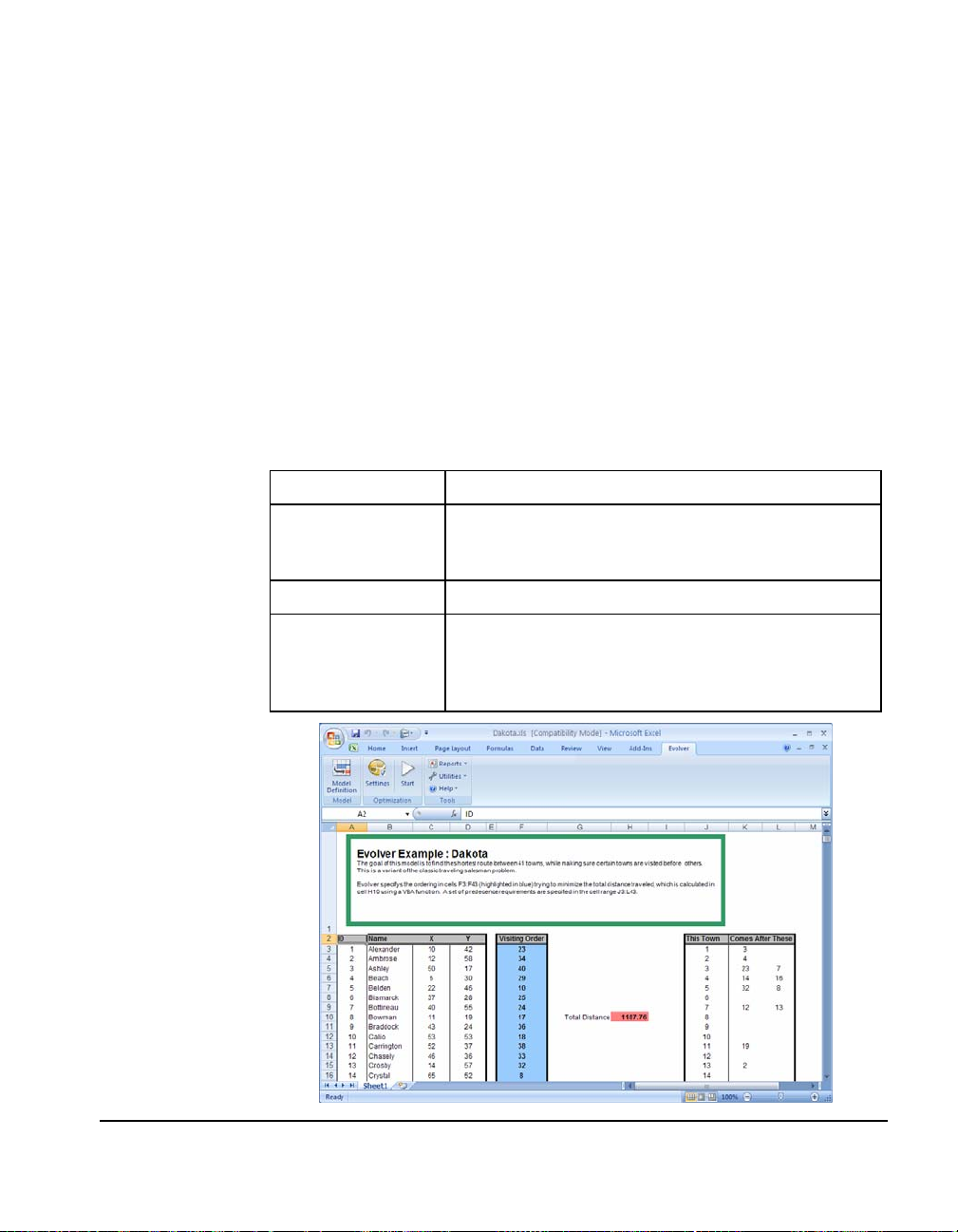
Dakota: Routing With Constraints
A real-estate firm needs to assess each of its properties throughout
North Dakota in a certain order, so that certain properties are visited
before others. Similar to the classic traveling salesman problem, the
goal of this problem is to find the shortest route among a set of cities
that ensures that each city is visited once. However, here we add the
constraint that certain cities must be visited before certain other cities
(such as town #2 coming after town #4). This means that instead of
the “order” solving method we will use the “project” solving method.
A project is an ordering for a set of tasks where certain tasks must
precede other tasks. You could use the “project” solving method, in
conjunction with your own custom functions, to find the best timing
for a project (based on a combination of any number of criteria, such
as time to finish, resource utilization, etc.).
Example file:
Goal:
Solving method:
Similar problems:
Dakota.xls
Plan a route among 41 towns in North Dakota which
finds the shortest route between all cities while
making sure some cities are visited before others.
project
Re-schedule a project to balance resource utilization.
Schedule the flow of jobs in a machine shop to reduce
total time while ensuring that some jobs are done
before others.
Chapter 4: Example Applications 63
Page 70
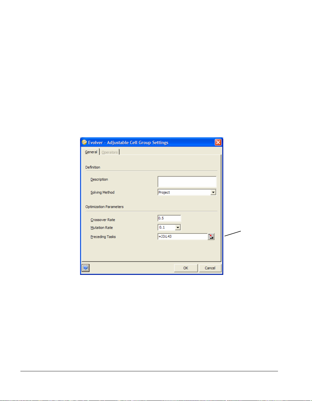
How The Model
Works
Cells F3:F43 contain the order in which the cities will be visited. Cell
H10 calculates the total length of the route, based on the order and the
x,y locations of the cities (in C3:D43). Cell H10 uses the custom
function “BigRouteLength” to speed up the computation of the total
route length.
Cells J3:L43 contain the precedence tasks. This is a table showing
which cities (tasks) must be preceded by other cities. Eight cities
(1,2,3,4,5,7, 11 and 13) must have certain cities that are visited before
them.
How To Solve It
Minimize the route length in H10 by changing the cells F3:F43. Use
the “project” solving method and set the precedence tasks to J3:L43.
These precedents are set in the Preceding Tasks field of the Adjustable
Cell Group Settings Dialog:
Precedent
Tasks
64 Dakota: Routing With Constraints
Page 71
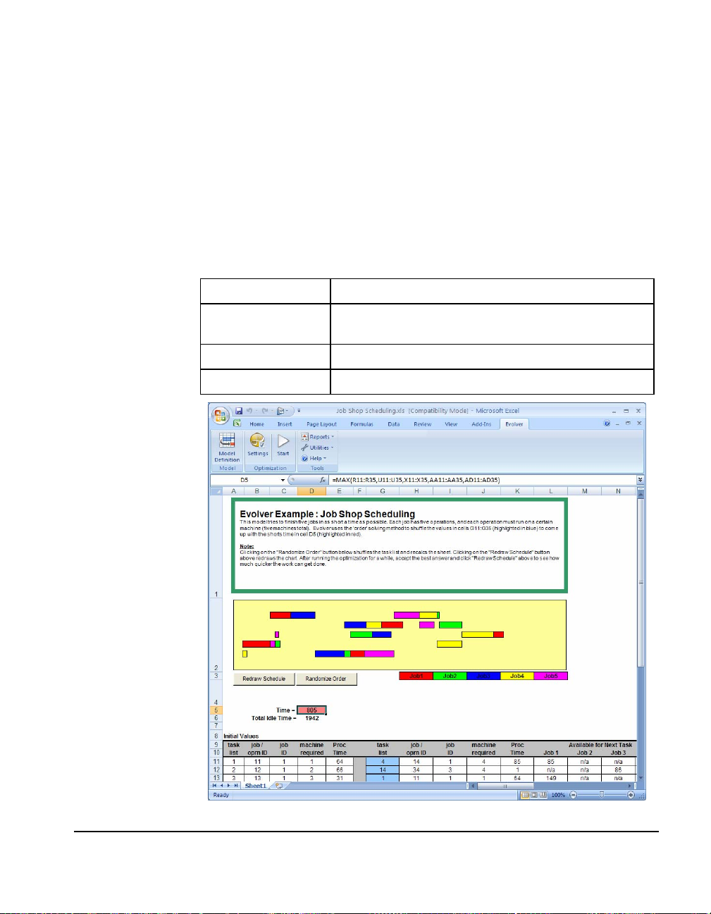
Job Shop Scheduling
A metalworking shop needs to find the best way to schedule a set of
jobs that can be broken down into steps that can be run on different
machines. Each job is composed of five tasks, and the tasks must be
completed in order. Each task must be done on a specific machine,
and takes a specific amount of time to complete. There are five jobs
and five machines.
Clicking the Draw Schedule button at the top of the sheet will redraw
the bar chart to show when each of the job tasks is scheduled to run.
Example file:
Goal:
Solving method:
Similar problems:
Job Shop Scheduling.xls
Assign job pieces (tasks) to machines so total time for
all jobs to finish is minimized.
order
Scheduling or project-management problems
Chapter 4: Example Applications 65
Page 72

How The Model
Works
Cell D5 computes the makespan, or how much time elapses between
the start of the first scheduled task and the end of the last scheduled
task. This total time is what we wish to minimize. Cells G11:G35
hold the variables (the tasks) to be shuffled to find the best
assignment order. The equations on the sheet figure out how soon
each task can run on the machine that it needs.
How To Solve It
Select a set of adjustable cells G11:G35 and select the order solving
method. Minimize cell D5.
66 Job Shop Scheduling
Page 73
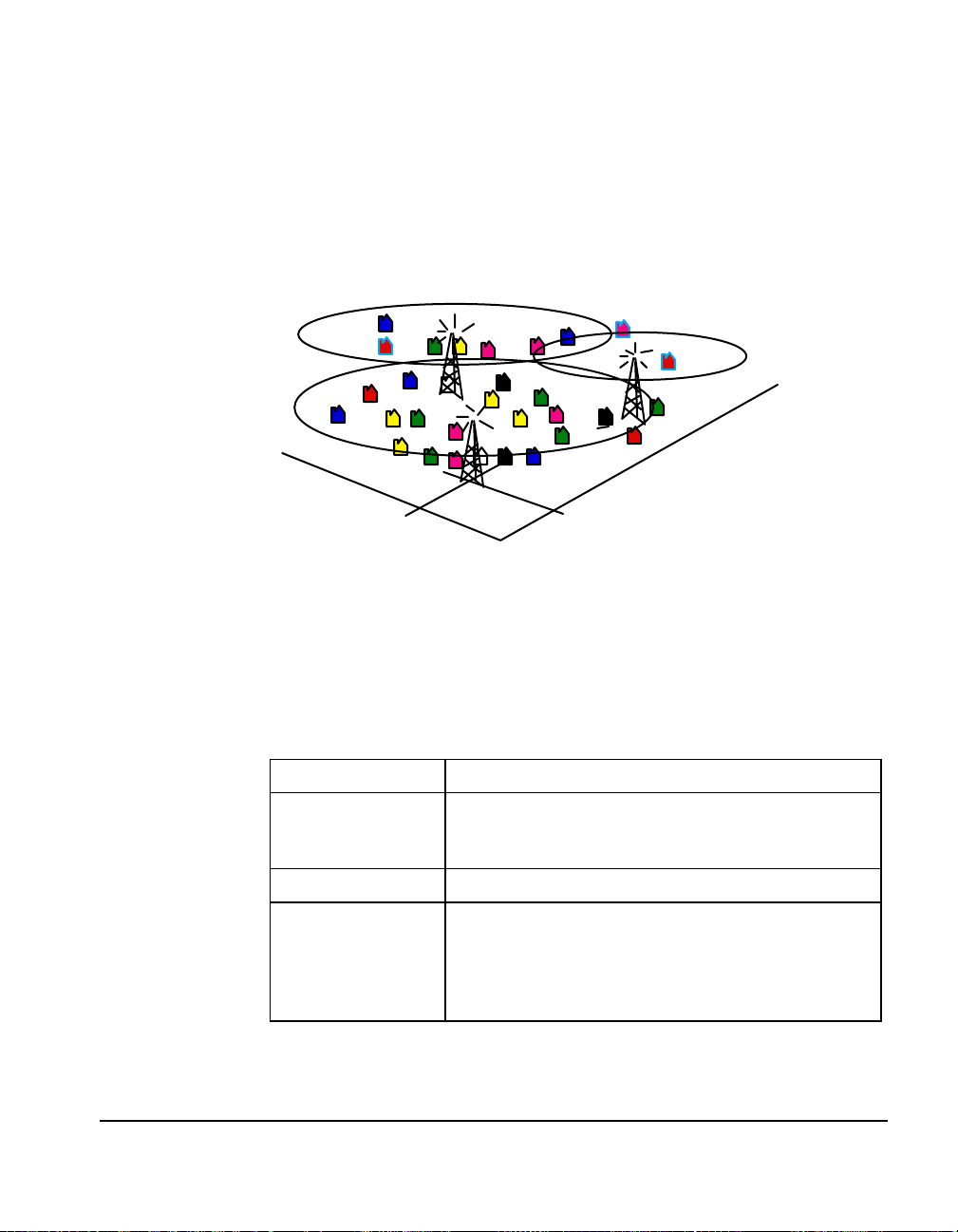
Radio Tower Location
A radio network wants to build three radio towers in a region that has
twelve major communities. Each community has a different
population size, and each radio tower has a different strength
broadcast range. The goal is to place the towers so that the maximum
number of potential listeners fall inside the broadcast radii of the
towers.
11
xy
A more complicated example of a location problem might be to locate
several factories so that they are a) in the vicinity of both vendors and
customers, b) in affordable, open land, and c) near a large, technically
trained work force. Any number of additional influences on the best
locations, such as tax incentives, can also be added to such a model.
Evolver can then find the best locations in x,y or even x,y,z coordinate
space.
Example file:
The Goal:
Solving method:
Similar problems:
Radio Tower Location.xls
Find the best x,y coordinates for three radio towers so
that the maximum potential listening population falls
inside their broadcasting range.
recipe
Find sites for warehouses that minimize the shipping
necessary between warehouses and stores. Locate fire
stations so that populations are best covered with a
limited number of stations, including factors such as
housing density.
Chapter 4: Example Applications 67
Page 74

How The Model
Works
The file “Radio Tower Location.xls” models a two-dimensional
landscape where the placement of five radio towers determines how
many listeners are reached. Cells C6:D8 contain the x,y coordinates
for the three towers. The illustration in the model consists of two
elements: one is a bitmap picture of the population densities (in
green) pasted from the Windows Paintbrush program; the other is an
Excel scatter graph that re-calculates automatically to show the
locations of the towers.
Ten communities are represented as single-point locations. The Excel
model computes the distance between the communities and the
towers in K4:M15 to determine if each community is covered (yes) or
not covered (no). The total population of all the covered communities
(the number we want to maximize) is calculated in cell O17.
How To Solve It
Maximize the population reached in cell O17 by adjusting the tower
location cells C6:D8. Use the “recipe” solving method and set the
ranges for the variables from 0 to 50 (the limits of our location area).
The “recipe” solving method tells Evolver to adjust the variables
chosen in any way it sees fit. As is the case with a recipe for baking,
we are trying to find the right mix of “ingredients” (x,y coordinates)
to produce the optimum solution.
68 Radio Tower Location
Page 75

Portfolio Balancing
A broker has a list of 80 securities, each worth a different amount of
money. The broker wants to group these securities into five packages
(portfolios) that are as close to each other in total value as possible.
This is an example of a general class of problems called bin packing
problems. Packing the holds of a cargo ship, so that each hold weighs
as much as the others is another example. If there are millions of
small items to be packaged into a few groups, such as grains of wheat
into ship holds, a roughly equal distribution can be guessed at
without a big difference in weight. However, several dozen packages
of different weights and/or sizes can be packed in very different
ways, and efficient packing can improve the balance that would be
found manually.
Example file:
Goal:
Solving method:
Similar problems:
Portfolio Balancing.xls
Break a list of securities up into five different
portfolios whose total values are as close as possible to
each other.
grouping
Create teams that have roughly equivalent collective
skills. Pack containers into holds of a ship so that the
weight is evenly distributed.
Chapter 4: Example Applications 69
Page 76

How The Model
Works
The “Portfolio Balancing.xls” file models a typical grouping
assignment. Column A contains identification numbers to specific
securities, and column B contains the dollar value of each security.
Column C assigns each security to one of the five portfolios. When
setting a grouping or bin packing type of problem and using the
grouping solving method, you must be sure that before you start
Evolver each group (1-5) is represented in the current scenario at least
once.
Cells F6:F10 calculate the total value of each of the five portfolios.
This is done with database criteria offscreen (in column I) and
“DSUM()” formulas in cells F6:F10. Thus, cell F6, for example,
calculates DSUM of all the values in column B that have been
assigned to group
5 (in column C).
Cell F12 computes the standard deviation among the total portfolio
values using the “STDEV()” function. This provides a measure of
how close in total value to each other the portfolios are. The graph
shows the total value of each portfolio, with a reference line drawn at
the goal number where each portfolio would be if they were all even.
How To Solve It
Minimize the value in cell F12 by adjusting the cells in C5:C104. Use
the “grouping” method and make sure the values 1, 2, 3, 4, and 5 each
appear at least once in column C.
The “grouping” solving method tells Evolver to arrange variables into
x groups, where x is the number of different values in the adjustable
cells at the start of an optimization.
70 Portfolio Balancing
Page 77

Portfolio Mix
A young couple has assets in many different types of investments,
each with its own yield, potential growth, and risk. By combining
several formulas which multiply various weights, they have
customized a sort of “score” which shows how well any particular
mix of investments satisfies their needs.
Example file:
The Goal:
Solving method:
Portfolio Mix.xls
Find the optimal mix of investments to maximize your
profit, given your current risk/return needs.
budget
How The Model
Works
This is a classic financial model which attempts to balance the risk of
loss against the return on investment. Each asset listed in column A is
assigned some weight in column C. The model multiplies the return
Chapter 4: Example Applications 71
Page 78

percentages by the weight each asset carries in the portfolio to yield a
total return in cell C18. We also calculate a total risk number in cell
C19, which should not be higher than the acceptable risk listed in cell
D19.
How To Solve It
The total “score” in cell C22 reflects the total return minus a penalty
for any risk above the acceptable percentage. We maximize this score.
72 Portfolio Mix
Page 79

Power Stations
A radio network buys three abandoned, non-working radio towers in
a region that has ten major communities. The network wants to
purchase brand new broadcast transmitters and install them in the
towers to get them broadcasting again.
Because there is a limited budget, the goal is to spend the least
amount of money on transmitters that will still cover all 9
surrounding communities. We assume a linear pricing model where
the cost of a transmitter is directly related to its power, so we’ll be
looking for the lowest amount of power to purchase, but it would be
just as easy to create a lookup chart of actual transmitter types and
prices.
Example file:
The Goal:
Solving method:
Similar problems:
Power Stations.xls
Find the smallest (cheapest) transmitter for each of the
old towers that will still cover the entire ten
surrounding communities.
recipe
set-covering problems, where a bunch of elements
need to be described by a small number of welldefined sets.
Chapter 4: Example Applications 73
Page 80
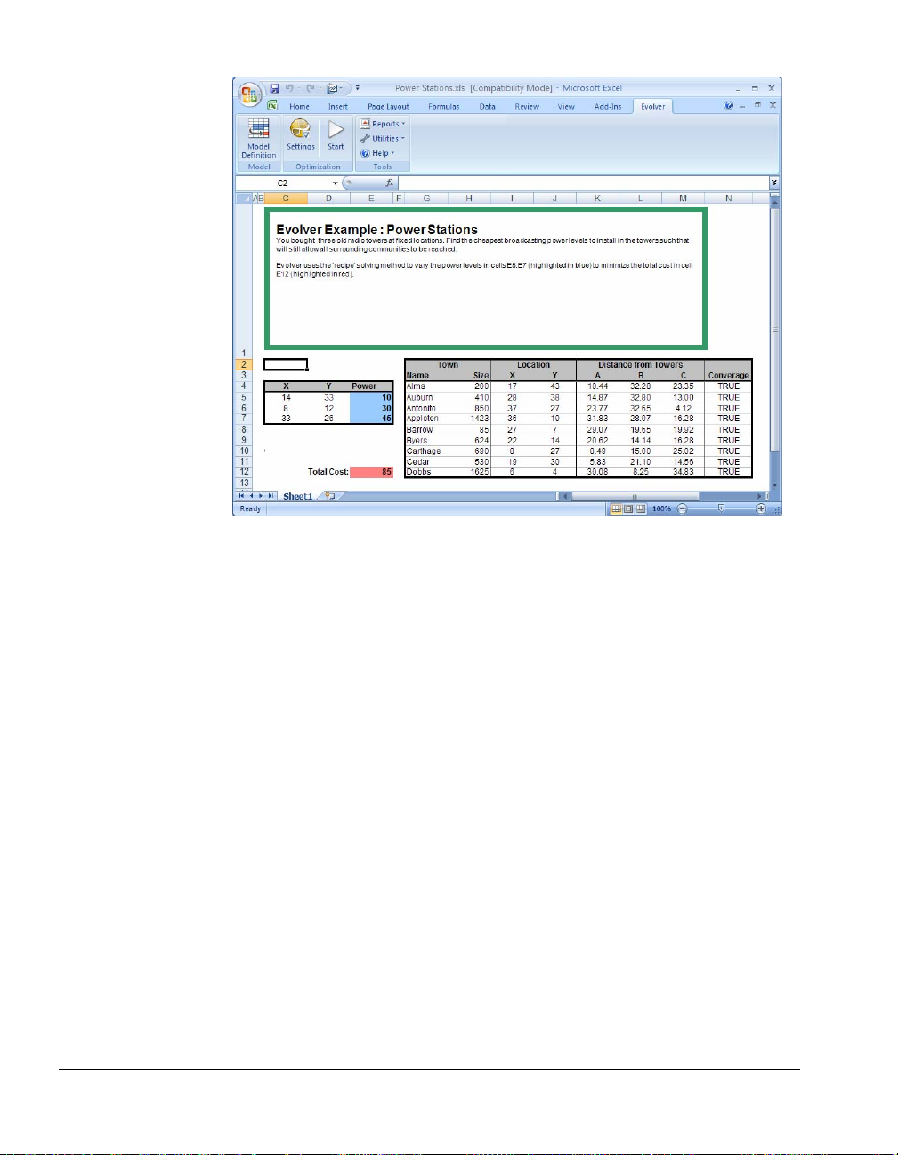
How The Model
Works
This is very similar to the radio tower location example (Radio Tower
Location.xls), except that here the locations are frozen, and it is the
tower’s power ranges in cells E5:E7 that are the variables to be
adjusted. We add up the power cost of the three towers in cell E12,
the target cell to be minimized.
Cells K4:M12 calculate how far away each community is from a
tower, and column N returns a TRUE if a community is near enough
to one of the transmitters to be covered. All of these constraints are
checked in a single hard constraint named All Areas Covered?. This
constraint has the formula AND($N$4:$N$12) which returns TRUE
only if all values in column N are TRUE.
How To Solve It
Minimize the power required in cell E12 by adjusting the radii of the
towers in cells E5:E7. Use the "recipe" solving method and set the
ranges for the variables from 0 to 100. The single hard constraint,
entered using the Excel formula format, is described above.
74 Power Stations
Page 81

Purchasing
Any time you have many possible ways to order items the quantity
discounts make it difficult to determine the most cost effective way to
buy the items. This model contains a simple price table, listing
quantity discount prices for a special solvent. You must buy at least
155 liters of this solvent, which comes in small, medium, large and
extra-large barrels.
Try to purchase the right number of each barrel size to minimize your
cost.
Example file:
The Goal:
Solving method:
Similar problems:
Purchasing.xls
Spend the least amount of money buying 155 liters of
solvent.
recipe
The opposite: create a pricing table that most
consistently and fairly rewards higher quantity orders.
Chapter 4: Example Applications 75
Page 82

How The Model
Works
This solvent comes in 3, 6, 10 and 14-liter barrels. The table of prices
for each size is listed in cells D6:H9. Cells H13:H16 contain the
amounts to buy of each size. Column K calculates the cost for each
purchase, and cell K18 is the total cost. This model allows you to
change the required amount to be purchased (cell I19) from 155 to
whatever you wish. Cell I18 contains the total liters that were
purchased, and so this cell must be at least the required number in
cell I19 (155). The single hard constraint is that the amount purchased
exceeds the amount required.
Since we need 155 liters, we might just think of buying 11 extra-large
barrels (154 liters), plus one small barrel (3 liters) for a total of 157
liters. According to the price table, that would cost $1,200 total. But
running the optimization will give you an even more cost-effective
combination.
How To Solve It
Minimize the cost in cell K18 by adjusting the quantities to buy in cell
H13:H16. Use the recipe solving method to adjust values, and set the
ranges of these variables to be between 1 and 20. You can not buy just
a part of one barrel, so we will ask Evolver to try only integers by
checking the “integers” option in the Adjustable Cells Dialog. Since
we cannot purchase less than 155 liters, enter a single hard constraint
specifying that I18>155.
76 Purchasing
Page 83
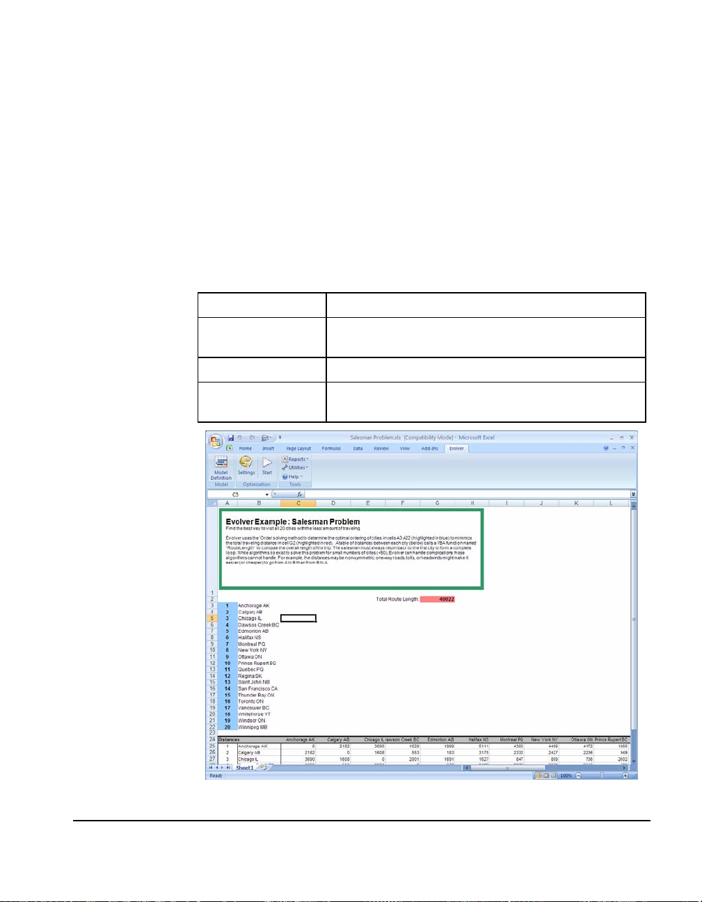
Salesman Problem
A salesman is required to visit every city in the assigned territory
once. What is the shortest route possible that visits every city? This is
a classic optimization problem and one that is extremely difficult for
conventional techniques to solve if there are a large (>50) number of
cities involved.
A similar problem might be finding the best order to perform tasks in
a factory. For example, it might be much easier to apply black paint
after applying white paint than the other way around. In Evolver,
these types of problems can be best solved by the order solving
method.
Example file:
Goal:
Solving method:
Similar problems:
Salesman Problem.xls
Find the shortest route among n cities that visits each
city once.
order
Plan the drilling of circuit board holes in the fastest
way.
Chapter 4: Example Applications 77
Page 84

How The Model
Works
The file “Salesman Problem.xls” calculates the route length of a trip to
various cities by looking up the distances in a table. Column A
contains identifying numbers for specific cities. Column B contains
the names that those numbers represent (with a lookup function).
The order in which the cities (and their numbers) appear from top to
bottom represents the order in which the cities are visited. For
example, if you entered a “9” into cell A3, then Ottawa would be the
first city visited. If A4 contained “6” (Halifax), then Halifax would be
the second city visited.
The distances between cities are represented in the table beginning at
C25. The distances in the table are symmetric (distance from A to B is
the same as from B to A). However, more realistic models may
include non-symmetric distances to represent greater difficulty of
traveling in one direction (because of tolls, available transportation,
headwinds, slope, etc.).
A function now must be used to calculate the length of the route
between these cities. The total route length will be stored in cell G2,
the cell we wish to optimize. To do this, we use the “RouteLength”
function. This is a custom VBA function in Salesman Problem.xls.
How To Solve It
Minimize the value in cell G2 by adjusting the cells in A3:A22. Use
the “order” method and make sure the values 1 through 20 exist in
the adjustable cells (A3:A22) before you start optimizing.
The “order” solving method tells Evolver to rearrange the chosen
variables, trying different permutations of existing variables.
78 Salesman Problem
Page 85
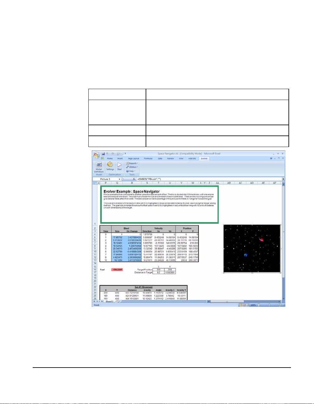
Space Navigator
As the launching crew of the space shuttle “Evolver III”, you must
figure out the amount and direction of each rocket thrust to reach
your destination using the least amount of fuel. The better solutions
will probably exploit the gravitational “whip” effect of nearby suns to
conserve fuel.
Example file:
Goal:
Solving method:
Similar problems:
Space Navigator.xls
Get a spaceship to its destination using as little fuel as
possible. Take advantage of the gravity of stars
moving through your neighborhood.
recipe
process control problems
How The Model
Works
Cells Q5:R15 hold the blast size and direction values for each of ten
time steps. Cell Q16, which we want to minimize, is simply the sum
of all the fuel burned in the ten time steps (Q4:Q13).
The hard constraints are: a) that the ship's final position be within 10
horizontal units of its destination, and b) that it be within 10 vertical
units.
Chapter 4: Example Applications 79
Page 86

How To Solve It
Minimize cell Q16. Create an adjustable cells group that uses the
recipe solving method using cells Q5:R13. The Blast cells (Q5:Q13)
should range between 0 and 300 and the Direction cells (R5:R13)
should range between -3 and 3, since it uses Radians to represent the
direction of the blasts. One Radian is about 57 degrees.
80 Space Navigator
Page 87
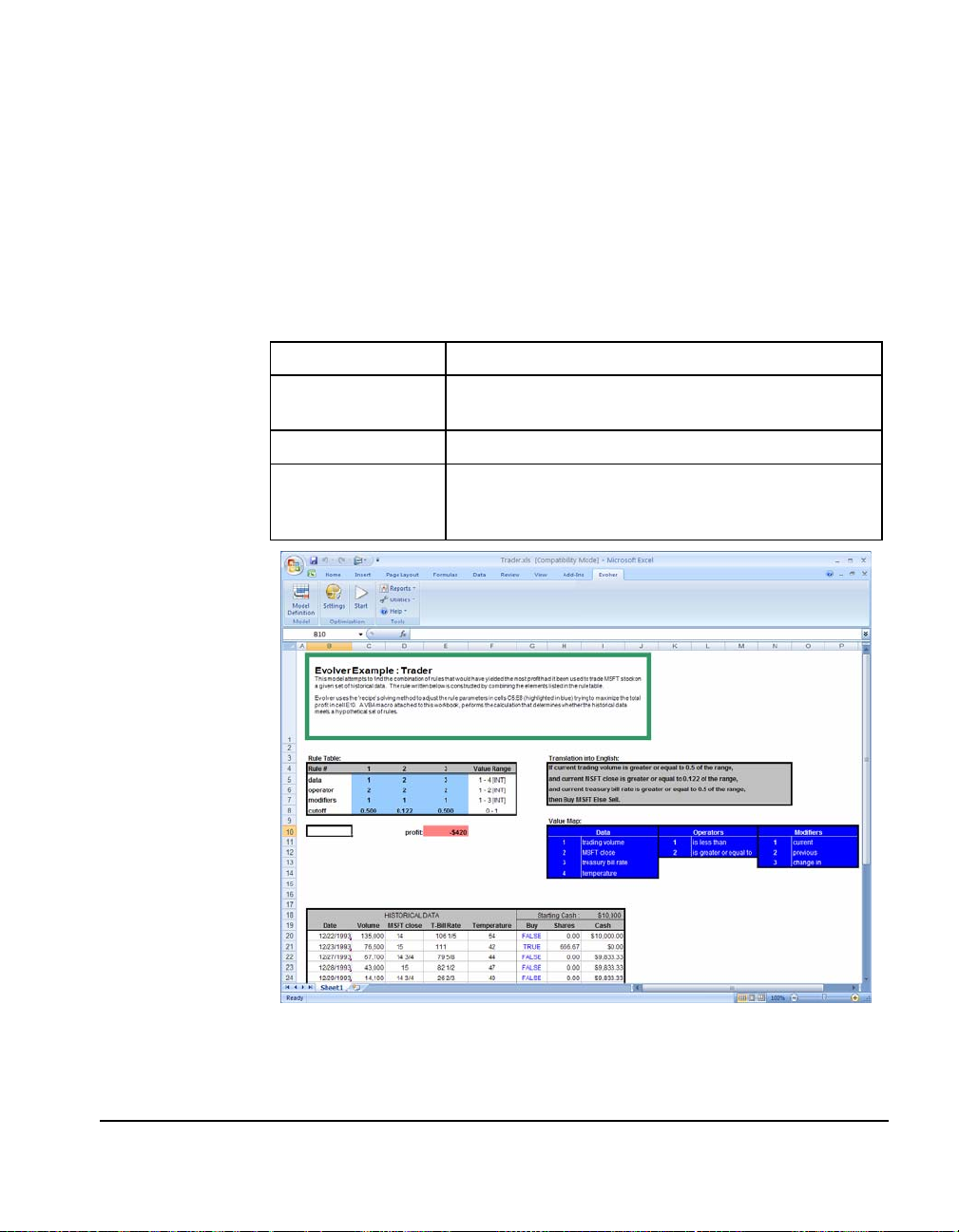
Trader
You are trading on the S&P 500, and you have determined that
technical analysis provides more accurate forecasting of stocks than
traditional fundamental analysis, and can save you time once you
build a system. It seems there are an infinite number of possible rules
by which you could trade, but only a few of them would have made
you a tidy profit if you had been following them. An intelligent
computer search could help you determine what rules would have
made the most money over a certain historical period.
Example file:
Goal:
Solving method:
Similar problems:
Trader.xls
Find a set of three rules which would have yielded the
highest return over a certain time period.
recipe
find optimal moving averages that would have
yielded the best result; any rule-finding or criteriafinding problems
Chapter 4: Example Applications 81
Page 88

How The Model
Works
This model uses several adjustable cell groups to solve the overall
problem. There are three rules that are evaluated for each trading
day. If the conditions of all three rules are true, then the computer
will buy on that day, otherwise it will sell. (A more realistic trading
system would not just buy or sell, but also sometimes hold onto what
it has.)
Each rule is described by a set of four numbers in cells C5:E8 which
indicate several things: 1) which data source the rule refers to, 2)
whether the data value should be above or below a cutoff value, 3) the
cutoff value that determines if the rule is true, and 4.) a modifier value
that determines if the value itself should be examined, or if the last
day's value or the change since the last day should be examined.
The cutoff values range from 0 to 1, and represent the percentage of
the data source's range. For example, if volume ranges from 5,000 to
10,000, then a cutoff value of 0.0 would match a volume of 5,000, a
cutoff value of 1.0 would match a volume of 10,000, and a cutoff value
of 0.5 would match a volume of 7,500. This system allows the rules to
refer to any data source, regardless of the values it takes on.
How To Solve It
Create adjustable cell groups, all using the “recipe” solving method.
Each row in C5:E5, C6:E6, C7:E7, and C8:E8 should be created
separately, so that each group can easily be assigned its own options
such as integer and ranges. The settings for each set of variables are
listed in F5:F8. Maximize on cell E10, which calls a macro to simulate
trading with those rules. The total profit made after simulating
trading on each day in the historical database is returned in cell E10.
82 Trader
Page 89
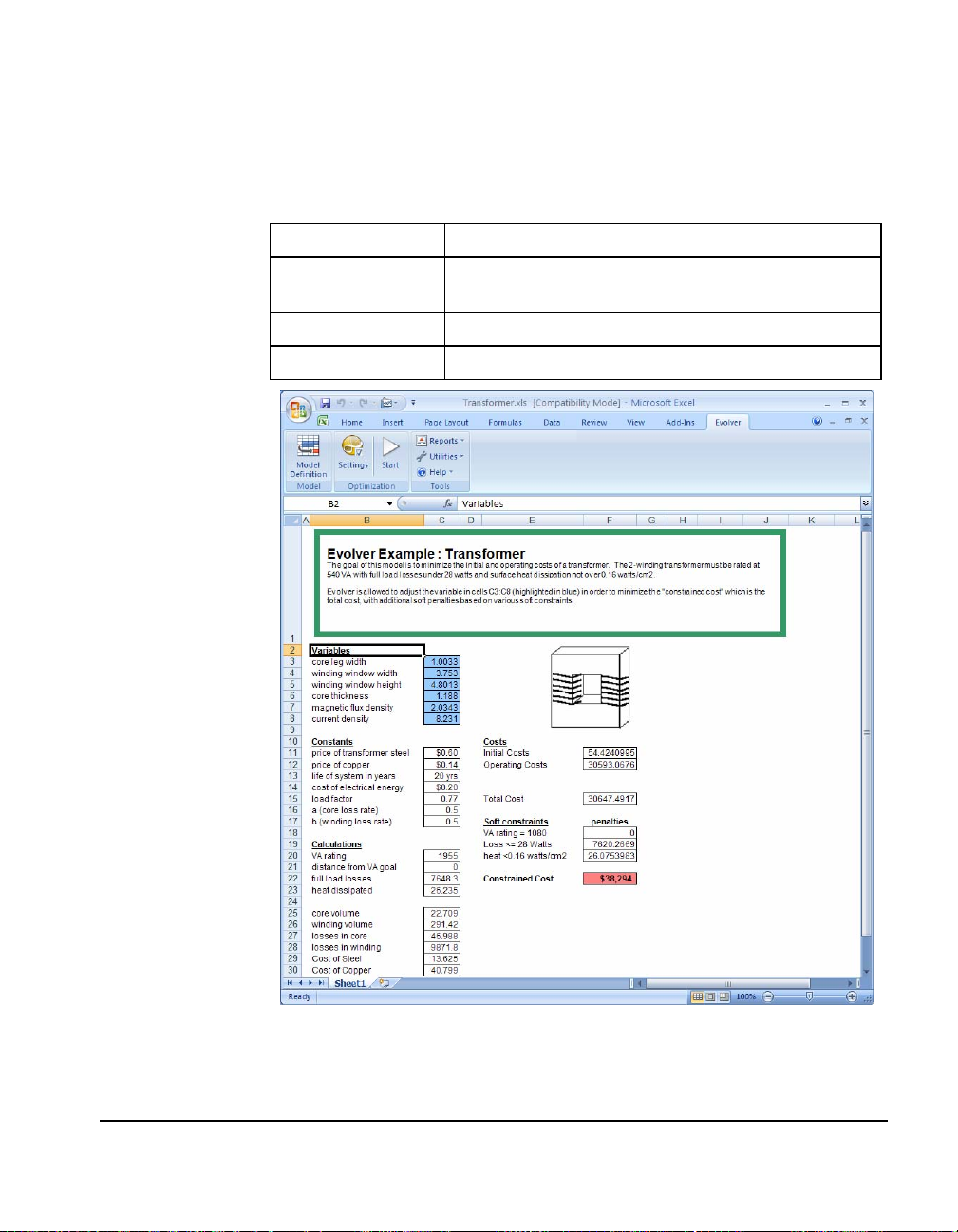
Transformer
The 2-winding transformer must be rated at 1080 VA with full load
losses under 28 watts and surface heat dissipation not over 0.16
watts/cm2. Minimize costs while observing the performance criteria.
Example file:
Goal:
Solving method:
Similar problems:
Transformer.xls
Minimize the initial and operating cost of a
transformer.
recipe
circuit design, bridge design
How The Model
Works
The rating, load loss, and heat dissipation constraints are coded as
soft constraints. We create a soft constraint by penalizing those
solutions which do not meet our requirements, and are invalid.
Unlike a hard constraint which must be met, Evolver is allowed to try
Chapter 4: Example Applications 83
Page 90

out some invalid solutions, but because these invalid solutions are
penalized by a function in your model which checks for violations,
they will produce poor results in your target cell. Thus, over time,
these invalid solutions will be discarded from the evolving
population of possible solutions.
A soft-constraint model may work better than a hard-constraint, if the
problem is less heavily constrained. It also allows Evolver to accept a
really great solution even if it may fall a little short of the constraints,
which could be more valuable than a not-so-great solution that meets
all the constraints.
How To Solve It
Compute material cost (initial cost) and operating costs (cost of
electricity * electricity wasted) in cells F11 and F12. Combine these
with penalty functions set in F18:F20 to form a final constrained cost
in cell F22. Minimize this target cell using the recipe solving method.
84 Transformer
Page 91

Transportation
How cheaply can we truck objects around the country? This standard
problem was expanded from an older Microsoft Solver example.
“Minimize the costs of shipping goods from production plants to
warehouses near metropolitan demand centers, while not exceeding
the supply available from each plant and meeting the demand from
each metropolitan area.”
To make the problem more realistic, the shipping costs were changed
so they are no longer linear, but depend on how many trucks are
needed. A truck can carry up to 6 objects, so shipping 14 objects
requires 3 trucks (carrying 6 + 6 + 2 objects).
Example file:
Goal:
Solving method:
Similar problems:
Transportation.xls
Truck objects from three plants to five warehouses in
the cheapest way possible.
recipe
design communications networks
Chapter 4: Example Applications 85
Page 92

How The Model
Works
Cells C5:G7 contain the number of objects shipped from each plant to
each warehouse. C13:G13 compute the number of trucks that would
be needed to ship those objects. The hard constraints are: 1) that the
total shipped from each plant is less than or equal to the supply on
hand at the plant, and 2) that the total shipped from all plants to each
warehouse is greater than or equal the amount that warehouse
requires. This ensures that every warehouse will get what it needs,
and no plant is overtaxed.
How To Solve It
Use the recipe solving method on cells C5:G7, using integers between
0 and 500. A set of hard constraints are entered for each plant
specifying that plant shipments<=plant supply. A second set of hard
constraints are entered for each warehouse specifying that total
shipments to warehouse>=warehouse demands. Minimize the
shipping cost in cell B22.
86 Transportation
Page 93

Chapter 5: Evolver Reference Guide
Model Definition Command.............................................................89
Adjustable Cell Ranges.........................................................................91
Adjustable Cell Groups ........................................................................93
Recipe Solving Method...........................................................95
Order Solving Method.............................................................96
Grouping Solving Method......................................................96
Budget Solving Method ..........................................................98
Project Solving Method...........................................................99
Schedule Solving Method.....................................................100
Crossover and Mutation Rate...............................................103
Number of Time Blocks and Constraint Cells..................104
Preceding Tasks ......................................................................104
Operators..................................................................................105
Constraints ............................................................................................107
Add - Adding Constraints.....................................................107
Simple and Formula Constraints.........................................108
Soft Constraints ......................................................................109
Optimization Settings Command..................................................113
Optimization Settings Command – General Tab...........................113
Optimization Settings Command – Runtime Tab .........................115
Optimization Runtime Options...........................................116
Optimization Settings Command – View Tab ...............................118
Optimization Settings Command – Macros Tab............................119
Start Optimization Command........................................................121
Utilities Commands........................................................................123
Application Settings Command........................................................123
Constraint Solver Command..............................................................124
Evolver Watcher..............................................................................127
Evolver Watcher – Progress Tab........................................................128
Evolver Watcher – Summary Tab......................................................130
Evolver Watcher – Log Tab.................................................................131
Chapter 5: Evolver Reference Guide 87
Page 94

Evolver Watcher – Population Tab................................................... 132
Evolver Watcher – Diversity Tab...................................................... 133
Evolver Watcher – Stopping Options Tab...................................... 134
88 Transportation
Page 95

Model Definition Command
Defines the goal, adjustable cells and constraints for a model
Selecting the Evolver Model Definition command (or clicking the
Model icon on the Evolver toolbar) displays the Model Dialog.
The Evolver Model Dialog is used to specify or describe an
optimization problem to Evolver. This dialog starts empty with each
new Excel workbook, but saves its information with each workbook.
That means that when the sheet is opened again, it will be filled out
the same way. Each component of the dialog is described in this
section.
Chapter 5: Evolver Reference Guide 89
The Evolver Model Dialog.
Page 96

Options in the Model dialog include:
• Optimization Goal. The Optimization Goal option determines
what kind of answer Evolver is to search for. If Minimum is
selected, Evolver will look for variable values that produce the
smallest possible value for the target cell (all the way down to 1e300). If Maximum is selected, Evolver will search for the
variable values that result in the largest possible value for the
target cell (up to +1e300).
If Target Value is selected, Evolver will search for variable values
that produce a value for the target cell as close as possible to the
value you specify. When Evolver finds a solution which produces
this result, it will automatically stop. For example, if you specify
that Evolver should find the result that is closest to 14, Evolver
might find scenarios that result in a value such as 13.7 or 14.5.
Note that 13.7 is closer to 14 than 14.5; Evolver does not care
whether the value is greater or less than the value you specify, it
only looks at how close the value is.
• Cell. The cell or target cell contains the output of your model. A
value for this target cell will be generated for each "trial solution"
that Evolver generates (i.e., each combination of possible
adjustable cell values). The target cell should contain a formula
which depends (either directly or through a series of calculations)
on the adjustable cells. This formula can be made with standard
Excel formulas such as SUM() or user-defined VBA macro
functions. By using VBA macro functions you can have Evolver
evaluate models that are very complex.
As Evolver searches for a solution it uses value of the target cell as
a rating or “fitness function” to evaluate how good each possible
scenario is, and to determine which variable values should
continue cross-breeding, and which should die. In biological
evolution, death is the “fitness function” that determines what
genes continue to flourish throughout the population. When you
build your model, your target cell must reflect the fitness or
“goodness” of any given scenario, so as Evolver calculates the
possibilities, it can accurately measure its progress.
90 Model Definition Command
Page 97
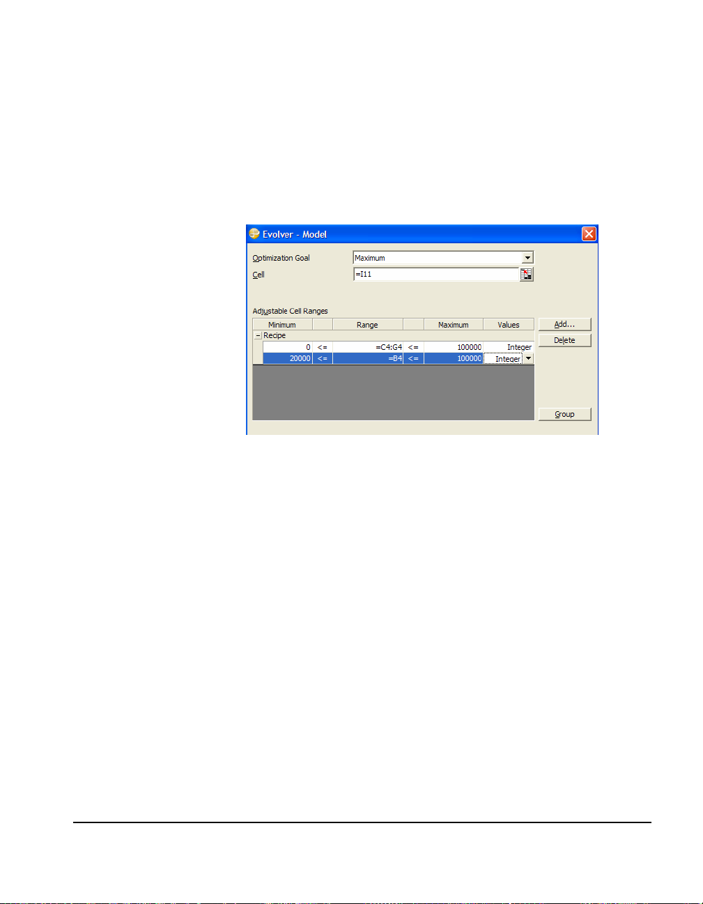
Adjustable Cell Ranges
The Adjustable Cell Ranges table displays each range which contains
the cells or values that Evolver can adjust, along with the description
entered for those cells. Each set of adjustable cells is listed in a
horizontal row. One or more adjustable cell ranges can be included in
an Adjustable Cell Group. All cell ranges in an Adjustable Cell
Group share a common solving method, crossover rate, mutation rate
and operators.
Because the adjustable cells contain the variables of the problem, you
must define at least one group of adjustable cells to use Evolver. Most
problems will be described with only one group of adjustable cells,
but more complex problems may require different blocks of variables
to be solved with different solving methods simultaneously. This
unique architecture allows for highly complex problems to be easily
built up from many groups of adjustable cells.
The following options are available for entering Adjustable Cell
Ranges:
• Add. You can add new adjustable cells by clicking on the “Add”
button next to the Adjustable Cells list box. Select the cell or cell
range to be added, and a new row will appear in the Adjustable
Cell Ranges table. In the table, you can enter a Minimum and
Maximum value for the cells in the range, along with the type of
Values to test – Integer values across the range, or Any values.
• Minimum and Maximum. After you have specified the location
of the adjustable cells, the Minimum and Maximum entries set the
range of acceptable values for each adjustable cell. By default,
each adjustable cell takes on a real-number (double-precision
floating point) value between -infinity and +infinity.
Chapter 5: Evolver Reference Guide 91
Page 98

Range settings are constraints that are strictly enforced. Evolver
will not allow any variable to take on a value outside the set
ranges. You are encouraged to set more specific ranges for your
variables whenever possible to improve Evolver’s performance.
For example, you may know that the number cannot be a
negative, or that Evolver should only try values between 50 and
70 for a given variable.
• Range. The reference for the cell(s) to be adjusted is entered in
the Range field. This reference can be entered by selecting the
region in the spreadsheet with the mouse, entering a range name
or typing in a valid Excel reference such as Sheet1!A1:B8. The
Range field is available for all solving methods. For recipe and
budget methods, however, Minimum, Maximum and Values
options can be added to allow the entry of a range for the
adjustable cells.
NOTE: By assigning tight ranges to your variables, you can limit
the scope of the search, and speed up Evolver’s convergence on a
solution. But be careful not to limit the ranges of your variables
too tightly; this may prevent Evolver from finding optimal
solutions.
• Values. The Values entry allows you to specify that Evolver
should treat all of the variables in the specified range as integers
(e.g., 22), rather than as real numbers (e.g., 22.395). This option is
only available when using the “recipe” and “budget” solving
methods. The default is to treat the variables as real numbers.
Be sure to turn on the Integers setting if your model uses variables to
lookup items from tables (HLOOKUP(), VLOOKUP(), INDEX(),
OFFSET(), etc.). Note that the Integers setting affects all
of the
variables in the selected range. If you want to treat some of your
variables as reals and some as integers, you can create two groups of
adjustable cells instead of one, and treat one block as integers and the
other block as reals. Simply “Add” a recipe group of adjustable cells,
and leave the Values entry as Any. Next, “Add” another cell range,
this time selecting the Integers setting and selecting only the integer
adjustable cells.
92 Model Definition Command
Page 99
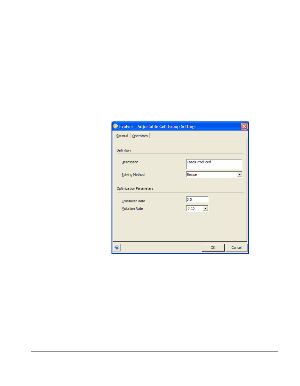
Adjustable Cell Groups
Each group of adjustable cells can contain multiple cell ranges. This
allows you to build a "hierarchy" of groups of cell ranges that are
related. Within each group, each cell range can have its own Min-Max
range constraint.
All cell ranges in an Adjustable Cell Group share a common solving
method, crossover rate, mutation rate and operators. These are
specified in the Adjustable Cell Group Settings dialog. This dialog
is accessed by clicking the Group button next to the Adjustable Cell
Ranges table. You may create a new Group to which you can add
adjustable cell ranges or edit the settings for an existing group.
Chapter 5: Evolver Reference Guide 93
Page 100

Options on the General tab in the Adjustable Cell Group Settings
dialog include:
• Description. Describes the group of adjustable cell ranges in
dialogs and reports.
• Solving Method. Selects the Solving Method to be used for each
of the adjustable cell ranges in the group.
When you select a range of cells to be adjusted by Evolver, you also
are specifying a “solving method” you wish to apply when adjusting
those adjustable cells. Each solving method is, in essence, a
completely different genetic algorithm, with its own optimized
selection, crossover and mutation routines. Each solving method
juggles the values of your variables a different way.
The “recipe” solving method, for example, treats each variable
selected as an ingredient in a recipe; each variable’s value can be
changed independently of the others’. In contrast, the “order” solving
method swaps values between the adjustable cells, reordering the
values that were originally there.
There are six solving methods that come with Evolver. Three of the
solving methods (recipe, order, and grouping) use entirely different
algorithms. The other three are descendants of the first three, adding
additional constraints.
The following section describes the function of each solving method.
To get a better understanding of how each solving method is used,
you are also encouraged to explore the example files included with
the software (see Chapter 4: Example Applications
94 Model Definition Command
).
 Loading...