OpenOffice 3.3 Calc Guide

OpenOffice.org 3.3

Calc Guide

Using Spreadsheets in OpenOffice.org 3.3

Copyright

This document is Copyright © 2005–2011 by its contributors as listed below. You may distribute it and/or modify it under the terms of either the GNU General Public License (http://www.gnu.org/licenses/gpl.html), version 3 or later, or the Creative Commons Attribution License (http://creativecommons.org/licenses/by/3.0/), version

3.0 or later. Note that Chapter 8, Using the DataPilot, is licensed under the Creative

Commons Attribution-Share Alike License, version 3.0.

Contributors

Rick Barnes Peter Kupfer Martin Fox James Andrew Krishna Aradhi Andy Brown Stephen Buck Bruce Byfield Nicole Cairns T. J. Frazier Stigant Fyrwitful Ingrid Halama Spencer E. Harpe Regina Henschel Peter Hillier-Brook John Kane Kirk Abbott Emma Kirsopp Jared Kobos Sigrid Kronenberger Shelagh Manton Alexandre Martins Kashmira Patel Anthony Petrillo Andrew Pitonyak Iain Roberts Hazel Russman Gary Schnabl Rob Scott Jacob Starr Sowbhagya Sundaresan Nikita Telang Barbara M Tobias John Viestenz Jean Hollis Weber Stefan Weigel Sharon Whiston Claire Wood Linda Worthington Michele Zarri Magnus Adielsson Sandeep Samuel Medikonda

Feedback

Please direct any comments or suggestions about this document to:

authors@documentation.openoffice.org

Publication date and software version

Published 18 April 2011. Based on OpenOffice.org 3.3.

You can download

an editable version of this document from

http://wiki.services.openoffice.org/wiki/Documentation/

Contents

Copyright................................................................................................................... 2

Note for Mac users.................................................................................................... 8

Chapter 1

Introducing Calc.......................................................................................................... 9

What is Calc?........................................................................................................... 10

Spreadsheets, sheets, and cells...............................................................................10

Parts of the main Calc window................................................................................10

Starting new spreadsheets...................................................................................... 18

Opening existing spreadsheets................................................................................20

Opening CSV files.................................................................................................... 21

Saving spreadsheets................................................................................................ 22

Password protection.................................................................................................24

Navigating within spreadsheets.............................................................................. 26

Selecting items in a sheet or spreadsheet...............................................................29

Working with columns and rows.............................................................................. 32

Working with sheets.................................................................................................33

Viewing Calc............................................................................................................ 34

Using the Navigator................................................................................................. 38

Using document properties......................................................................................40

Chapter 2

Entering, Editing, and Formatting Data....................................................................43

Introduction............................................................................................................. 44

Entering data using the keyboard...........................................................................44

Speeding up data entry............................................................................................46

Sharing content between sheets.............................................................................. 49

Validating cell contents............................................................................................ 50

Editing data.............................................................................................................. 52

Formatting data....................................................................................................... 53

Autoformatting cells and sheets..............................................................................59

Formatting spreadsheets using themes...................................................................60

Using conditional formatting...................................................................................60

Hiding and showing data.........................................................................................61

Sorting records........................................................................................................ 63

Finding and replacing in Calc.................................................................................. 65

Chapter 3

Creating Charts and Graphs......................................................................................69

Introduction............................................................................................................. 70

Creating a chart....................................................................................................... 70

Editing charts...........................................................................................................74

Formatting charts.................................................................................................... 79

Formatting 3D charts............................................................................................... 82

Formatting the chart elements................................................................................85

OpenOffice.org 3.3 Calc Guide 3

Adding drawing objects to charts............................................................................87

Resizing and moving the chart................................................................................ 88

Gallery of chart types............................................................................................... 89

Chapter 4

Using Styles and Templates in Calc...........................................................................98

What is a template?................................................................................................. 99

What are styles?....................................................................................................... 99

Types of styles in Calc..............................................................................................99

Accessing styles..................................................................................................... 100

Applying cell styles................................................................................................ 101

Applying page styles.............................................................................................. 102

Modifying styles..................................................................................................... 103

Creating new (custom) styles.................................................................................106

Copying and moving styles....................................................................................107

Deleting styles....................................................................................................... 109

Creating a spreadsheet from a template...............................................................109

Creating a template............................................................................................... 110

Editing a template.................................................................................................. 111

Adding templates using the Extension Manager...................................................113

Setting a default template..................................................................................... 113

Associating a spreadsheet with a different template.............................................114

Organizing templates.............................................................................................115

Chapter 5

Using Graphics in Calc.............................................................................................117

Graphics in Calc..................................................................................................... 118

Adding graphics (images)...................................................................................... 118

Modifying images...................................................................................................123

Using the picture context menu.............................................................................128

Using Calc’s drawing tools.................................................................................... 130

Positioning graphics...............................................................................................133

Creating an image map.......................................................................................... 136

Chapter 6

Printing, Exporting, and E-mailing..........................................................................138

Quick printing........................................................................................................ 139

Controlling printing............................................................................................... 139

Using print ranges................................................................................................. 142

Page breaks............................................................................................................ 145

Printing options setup in page styles..................................................................... 146

Headers and footers............................................................................................... 148

Exporting to PDF................................................................................................... 151

Exporting to XHTML.............................................................................................. 157

Saving as Web pages (HTML)................................................................................157

E-mailing spreadsheets.......................................................................................... 157

Digital signing of documents.................................................................................157

4 OpenOffice.org 3.3 Calc Guide

Removing personal data........................................................................................ 158

Chapter 7

Using Formulas and Functions................................................................................159

Introduction........................................................................................................... 160

Setting up a spreadsheet....................................................................................... 160

Creating formulas.................................................................................................. 161

Understanding functions........................................................................................175

Strategies for creating formulas and functions.....................................................180

Finding and fixing errors.......................................................................................182

Examples of functions............................................................................................187

Using regular expressions in functions..................................................................191

Advanced functions................................................................................................ 192

Chapter 8

Using the DataPilot.................................................................................................. 193

Introduction........................................................................................................... 194

Examples with step by step descriptions...............................................................194

DataPilot functions in detail...................................................................................214

Function GETPIVOTDATA...................................................................................... 236

Chapter 9

Data Analysis........................................................................................................... 240

Introduction........................................................................................................... 241

Consolidating data................................................................................................. 241

Creating subtotals.................................................................................................. 243

Using “what if” scenarios...................................................................................... 245

Using other “what if” tools.................................................................................... 249

Working backwards using Goal Seek.....................................................................254

Using the Solver.....................................................................................................256

Chapter 10

Linking Calc Data...................................................................................................... 259

Why use multiple sheets?.......................................................................................260

Setting up multiple sheets.....................................................................................260

Referencing other sheets in the spreadsheet........................................................ 263

Referencing other documents: links to sheets in other spreadsheets...................266

Hyperlinks and URLs............................................................................................. 267

Linking to external data.........................................................................................270

Linking to registered data sources........................................................................274

Embedding spreadsheets....................................................................................... 278

Chapter 11

Sharing and Reviewing Documents..........................................................................283

Introduction........................................................................................................... 284

Sharing documents (collaboration)........................................................................ 284

Recording changes.................................................................................................286

Adding comments to changes................................................................................288

Adding other comments......................................................................................... 290

OpenOffice.org 3.3 Calc Guide 5

Reviewing changes................................................................................................ 291

Merging documents............................................................................................... 294

Comparing documents........................................................................................... 295

Saving versions...................................................................................................... 295

Chapter 12

Calc Macros............................................................................................................ 298

Introduction........................................................................................................... 299

Using the macro recorder...................................................................................... 299

Write your own functions.......................................................................................303

Accessing cells directly.......................................................................................... 310

Sorting................................................................................................................... 311

Conclusion..............................................................................................................312

Chapter 13

Calc as a Simple Database.......................................................................................313

Introduction........................................................................................................... 314

Associating a range with a name........................................................................... 315

Sorting................................................................................................................... 320

Filters..................................................................................................................... 322

Calc functions similar to database functions.........................................................330

Database-specific functions................................................................................... 339

Conclusion..............................................................................................................340

Chapter 14

Setting up and Customizing Calc.............................................................................341

Introduction........................................................................................................... 342

Choosing options that affect all of OOo.................................................................342

Choosing options for loading and saving documents.............................................347

Choosing options for Calc...................................................................................... 350

Controlling Calc’s AutoCorrect functions.............................................................. 358

Customizing the user interface.............................................................................. 358

Adding functionality with extensions..................................................................... 366

Appendix A

Keyboard Shortcuts..................................................................................................369

Introduction........................................................................................................... 370

Navigation and selection shortcuts........................................................................370

Function and arrow key shortcuts.........................................................................371

Cell formatting shortcuts.......................................................................................373

DataPilot shortcuts................................................................................................ 374

Appendix B

Description of Functions..........................................................................................375

Functions available in Calc.................................................................................... 376

Mathematical functions......................................................................................... 376

Financial analysis functions................................................................................... 381

Statistical analysis functions..................................................................................393

Date and time functions......................................................................................... 401

6 OpenOffice.org 3.3 Calc Guide

Logical functions.................................................................................................... 404

Informational functions.......................................................................................... 405

Database functions................................................................................................ 407

Array functions...................................................................................................... 408

Spreadsheet functions...........................................................................................410

Text functions......................................................................................................... 414

Add-in functions..................................................................................................... 417

Appendix C

Calc Error Codes...................................................................................................... 421

Introduction to Calc error codes............................................................................ 422

Error codes displayed within cells.........................................................................423

General error codes...............................................................................................424

Index.......................................................................................................................... 427

OpenOffice.org 3.3 Calc Guide 7

Note for Mac users

Some keystrokes and menu items are different on a Mac from those used in Windows and Linux. The table below gives some common substitutions for the instructions in this chapter. For a more detailed list, see the application Help.

Windows/Linux Mac equivalent Effect

Tools > Options

menu selection

OpenOffice.org > Preferences

Access setup options

Right-click Control+click Open context menu

Ctrl (Control) z (Command) Used with other keys

F5 Shift+z+F5 Open the Navigator

F11 z+T Open Styles & Formatting window

8 OpenOffice.org 3.3 Calc Guide

Chapter 1

Introducing Calc

What is Calc?

Calc is the spreadsheet component of OpenOffice.org (OOo). You can enter data (usually numerical) in a spreadsheet and then manipulate this data to produce certain results.

Alternatively, you can enter data and then use Calc in a ‘What if...’ manner by changing some of the data and observing the results without having to retype the entire spreadsheet or sheet.

Other features provided by Calc include:

• Functions, which can be used to create formulas to perform complex

calculations on data

• Database functions, to arrange, store, and filter data

• Dynamic charts; a wide range of 2D and 3D charts

• Macros, for recording and executing repetitive tasks; scripting languages

supported include OpenOffice.org Basic, Python, BeanShell, and JavaScript

• Ability to open, edit, and save Microsoft Excel spreadsheets

• Import and export of spreadsheets in multiple formats, including HTML, CSV,

PDF, and PostScript

Note

If you want to use macros written in Microsoft Excel using the VBA macro code in OOo, you must first edit the code in the OOo Basic IDE editor. See Chapter 12 (Calc Macros).

Spreadsheets, sheets, and cells

Calc works with elements called spreadsheets. Spreadsheets consist of a number of individual sheets, each sheet containing cells arranged in rows and columns. A particular cell is identified by its row number and column letter.

Cells hold the individual elements—text, numbers, formulas, and so on—that make up the data to display and manipulate.

Each spreadsheet can have many sheets, and each sheet can have many individual cells. In Calc 3.3, each sheet can have a maximum of 1,048,576 (65,536 rows in Calc

3.2 and earlier) and a maximum of 1024 columns

Parts of the main Calc window

When Calc is started, the main window looks similar to Figure 1.

Note

If any part of the Calc window in Figure 1 is not shown, you can display it using the View menu. For example, View > Status Bar will toggle (show or hide) the Status Bar. It is not always necessary to display all the parts, as shown; show or hide any of them, as desired.

10 OpenOffice.org 3.3 Calc Guide

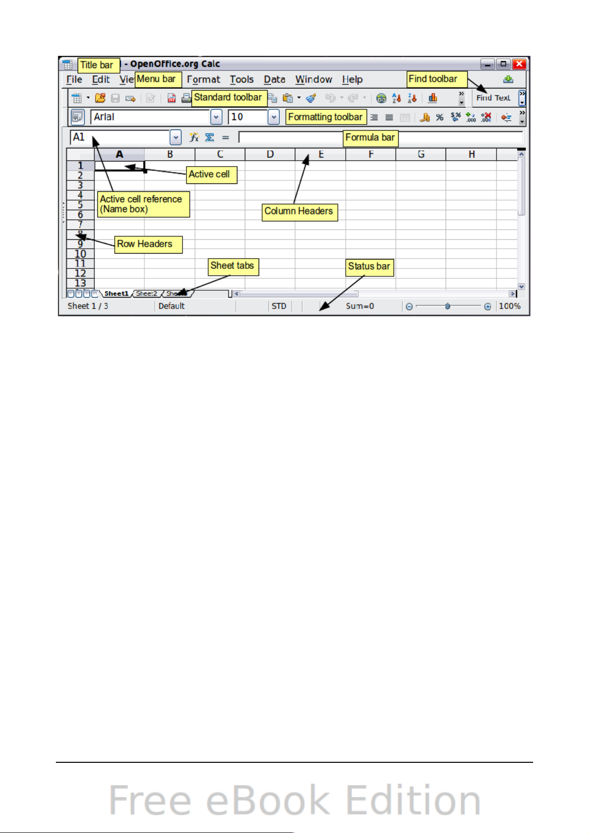
Figure 1: Parts of the Calc window

Title bar

The Title bar, located at the top, shows the name of the current spreadsheet. When the spreadsheet is newly created, its name is Untitled X, where X is a number. When you save a spreadsheet for the first time, you are prompted to enter a name of your choice.

Menu bar

Under the Title bar is the Menu bar. When you choose one of the menus, a submenu appears with other options. You can modify the Menu bar, as discussed in Chapter 14 (Setting Up and Customizing Calc).

• File contains commands that apply to the entire document such as Open,

Save, Wizards, Export as PDF, and Digital Signatures.

• Edit contains commands for editing the document such as Undo, Changes,

Compare Document, and Find and Replace.

• View contains commands for modifying how the Calc user interface looks such

as Toolbars, Full Screen, and Zoom.

• Insert contains commands for inserting elements such as cells, rows,

columns, sheets, and pictures into a spreadsheet.

• Format contains commands for modifying the layout of a spreadsheet such as

Styles and Formatting, Paragraph, and Merge Cells.

• Tools contains functions such as Spelling, Share Document, Cell Contents,

Gallery, and Macros.

• Data contains commands for manipulating data in your spreadsheet such as

Define Range, Sort, Filter, and DataPilot.

Chapter 1 Introducing Calc 11

• Window contains commands for the display window such as New Window,

Split, and Freeze.

• Help contains links to the Help file bundled with the software, What's This?,

Support, Registration, and Check for Updates.

Toolbars

Calc has several types of toolbars: docked (fixed in place), floating, and tear-off. Docked toolbars can be moved to different locations or made to float, and floating toolbars can be docked.

Four toolbars are located under the Menu bar by default: the Standard toolbar, the Find toolbar, the Formatting toolbar, and the Formula Bar.

The icons (buttons) on these toolbars provide a wide range of common commands and functions. You can also modify these toolbars, as discussed in Chapter 14 (Setting Up and Customizing Calc).

Placing the mouse pointer over any of the icons displays a small box, called a tooltip. It gives a brief explanation of the icon’s function. For a more detailed explanation, choose Help > What’s This? and hover the mouse pointer over the icon. To turn this feature off again, click once or press the Esc key twice. Tips and extended tips can be turned on or off from Tools > Options > OpenOffice.org > General.

Displaying or hiding toolbars

To display or hide toolbars, choose View > Toolbars, then click on the name of a toolbar in the list. An active toolbar shows a check mark beside its name. Tear-off toolbars are not listed in the View menu.

Palettes and tear-off toolbars

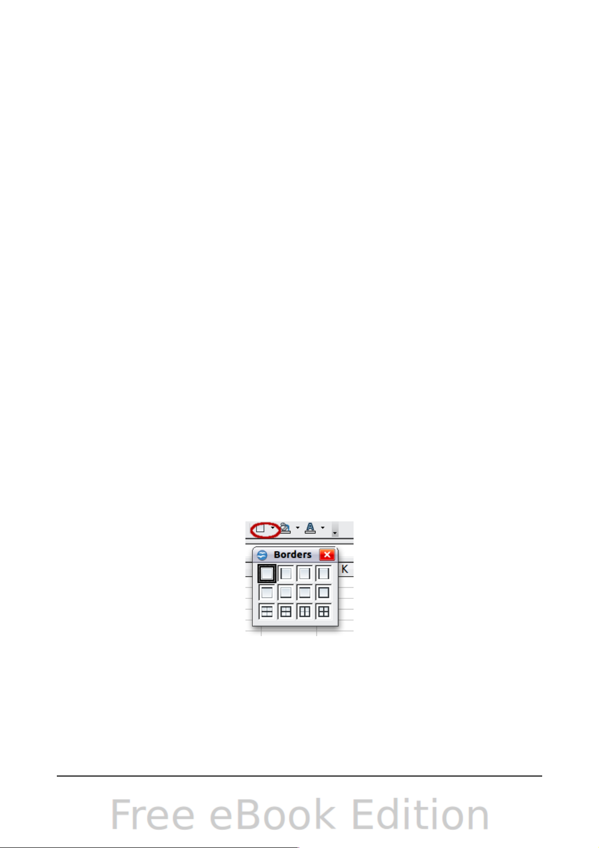
Toolbar icons with a small triangle to the right will display palettes, tear-off toolbars, and other ways of selecting things, depending on the icon.

An example of a palette is shown in Figure 2. It is displayed by clicking the small triangle to the right of the Borders toolbar icon.

An example of a tear-off toolbar is shown in Figure 3. Tear-off toolbars can be floating or docked along an edge of the screen or in one of the existing toolbar areas. To move a floating tear-off toolbar, drag it by the title bar.

12 OpenOffice.org 3.3 Calc Guide

Figure 2: Toolbar palette

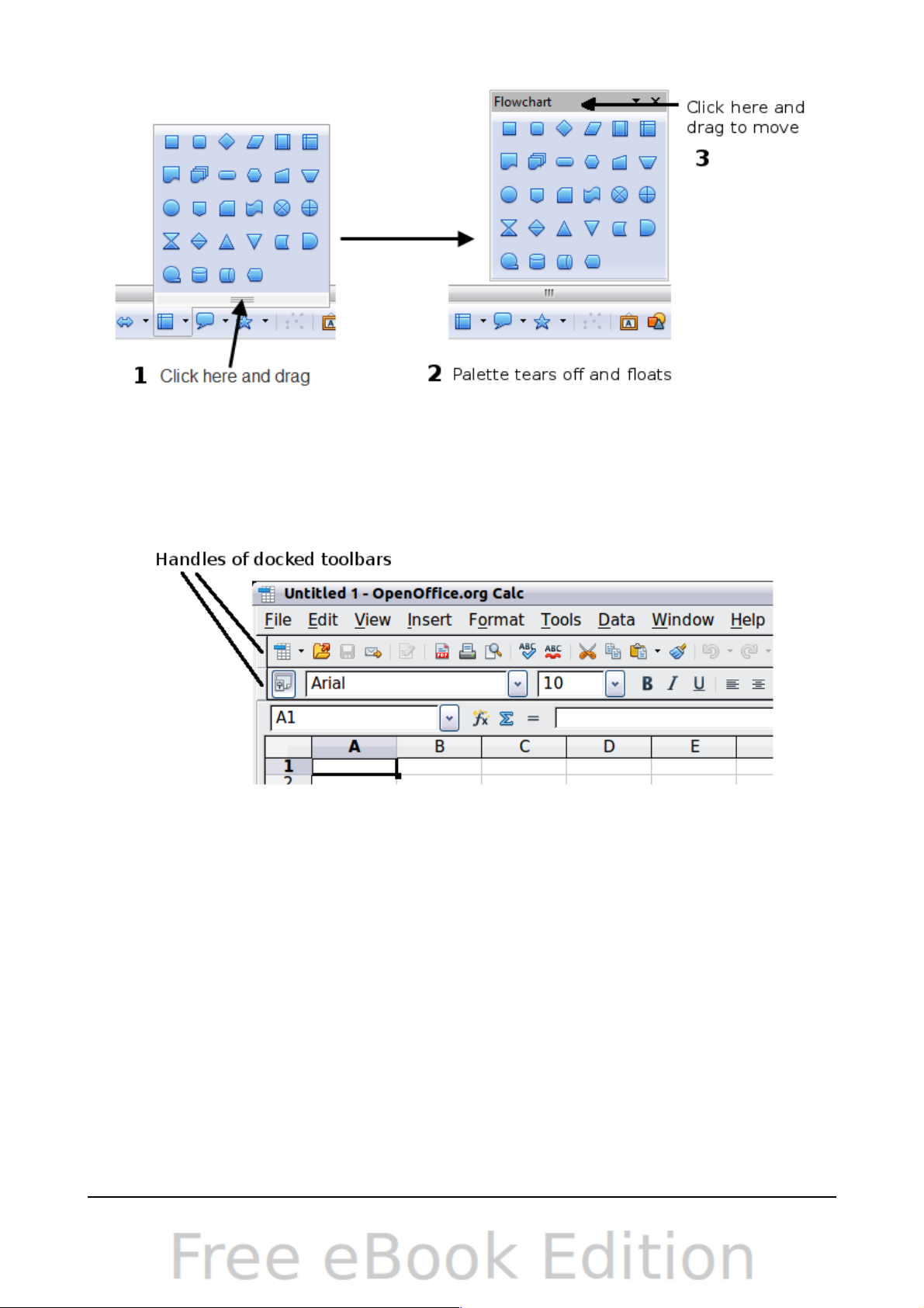
Figure 3: Example of a tear-off toolbar

Moving toolbars

To move a docked toolbar, place the mouse pointer over the toolbar handle, hold down the left mouse button, drag the toolbar to the new location, and then release the mouse button.

To move a floating toolbar, click on its title bar and drag it to a new location, as shown in Figure 3.

Docking/floating windows and toolbars

Toolbars and some windows, such as the Navigator and the Styles and Formatting window, are dockable. You can move, resize, or dock them to an edge.

To dock a window or toolbar, hold down the Control key and double-click on the frame of the floating window (or in a vacant area near the icons at the top of the floating window) to dock it in its last position.

To undock a window, hold down the Control key and double-click on the frame (or a vacant area near the icons at the top) of the docked window.

Chapter 1 Introducing Calc 13

Figure 4: Moving a docked toolbar

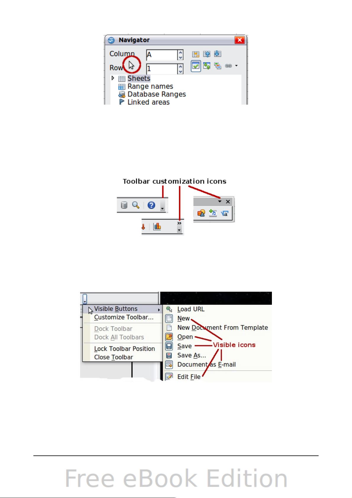
Figure 5: Control+double-click to dock or undock

Customizing toolbars

You can customize toolbars in several ways, including choosing which icons are visible and locking the position of a docked toolbar.

To access a toolbar’s customization options, use the down-arrow at the end of the toolbar or on its title bar (Figure 6).

To show or hide icons defined for the selected toolbar, choose Visible Buttons from the drop-down menu. Visible icons are indicated by a border around the icon (Figure

7). Click on icons to hide or show them on the toolbar.

You can also add icons and create new toolbars, as described in Chapter 16.

Formatting toolbar

In the Formatting toolbar, the three boxes on the left are the Apply Style, Font Name, and Font Size lists (see Figure 8). They show the current settings for the

selected cell or area. (The Apply Style list may not be visible by default.) Click the down-arrow to the right of each box to open the list.

14 OpenOffice.org 3.3 Calc Guide

Figure 6: Customizing toolbars

Figure 7: Selection of visible toolbar icons

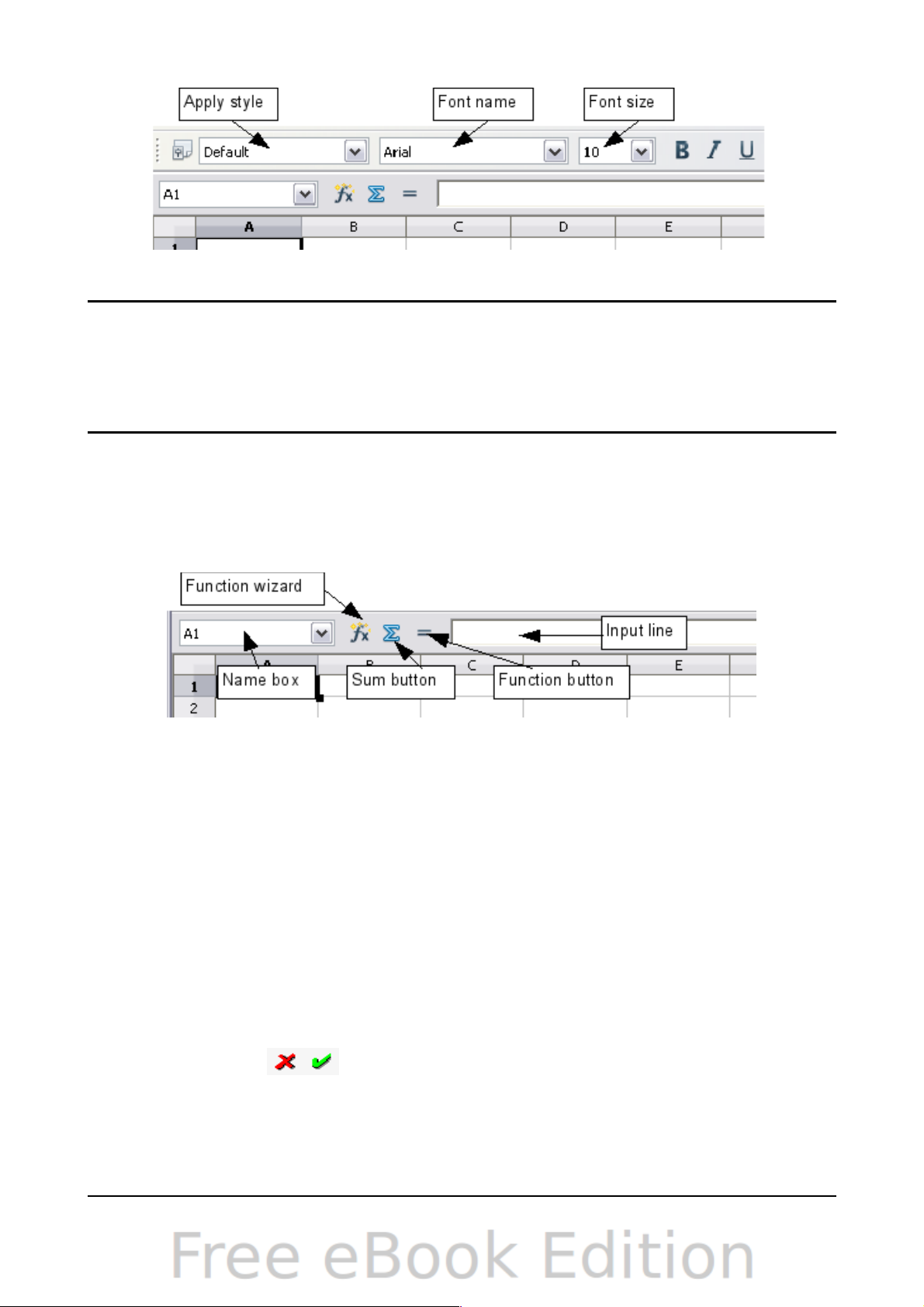
Figure 8: Apply Style, Font Name and Font Size lists

Note

If any of the icons (buttons) in Figure 8 is not shown, you can display it by clicking the small triangle at the right end of the Formatting toolbar, selecting Visible Buttons in the drop-down menu, and selecting the desired icon (for example, Apply Style) in the drop-down list. It is not always necessary to display all the toolbar buttons, as shown; show or hide any of them, as desired.

Formula Bar

On the left hand side of the Formula Bar is a small text box, called the Name Box, with a letter and number combination in it, such as D7. This combination, called the cell reference, is the column letter and row number of the selected cell.

To the right of the Name Box are the Function Wizard, Sum, and Function buttons.

Clicking the Function Wizard button opens a dialog from which you can search through a list of available functions. This can be very useful because it also shows how the functions are formatted.

In a spreadsheet the term function covers much more than just mathematical functions. See Chapter 7 (Using Formulas and Functions) for more details.

Clicking the Sum button inserts a formula into the current cell that totals the numbers in the cells above the current cell. If there are no numbers above the current cell, then the cells to the left are placed in the Sum formula.

Clicking the Function button inserts an equals (=) sign into the selected cell and the Input line, thereby enabling the cell to accept a formula.

When you enter new data into a cell, the Sum and Equals buttons change to Cancel and Accept buttons .

The contents of the current cell (data, formula, or function) are displayed in the Input line, which is the remainder of the Formula Bar. You can either edit the cell contents of the current cell there, or you can do that in the current cell. To edit inside

Chapter 1 Introducing Calc 15

Figure 9: Formula Bar

the Input line area, click in the area, then type your changes. To edit within the current cell, just double-click the cell.

Right-click (context) menus

Right-click on a cell, graphic, or other object to open a context menu. Often the context menu is the fastest and easiest way to reach a function. If you’re not sure where in the menus or toolbars a function is located, you may be able to find it by right-clicking.

Individual cells

The main section of the screen displays the cells in the form of a grid, with each cell being at the intersection of a column and a row.

At the top of the columns and at the left end of the rows are a series of gray boxes containing letters and numbers. These are the column and row headers. The columns start at A and go on to the right, and the rows start at 1 and go down.

These column and row headers form the cell references that appear in the Name Box on the Formula Bar (see Figure 9). You can turn these headers off by selecting View > Column & Row Headers.

Sheet tabs

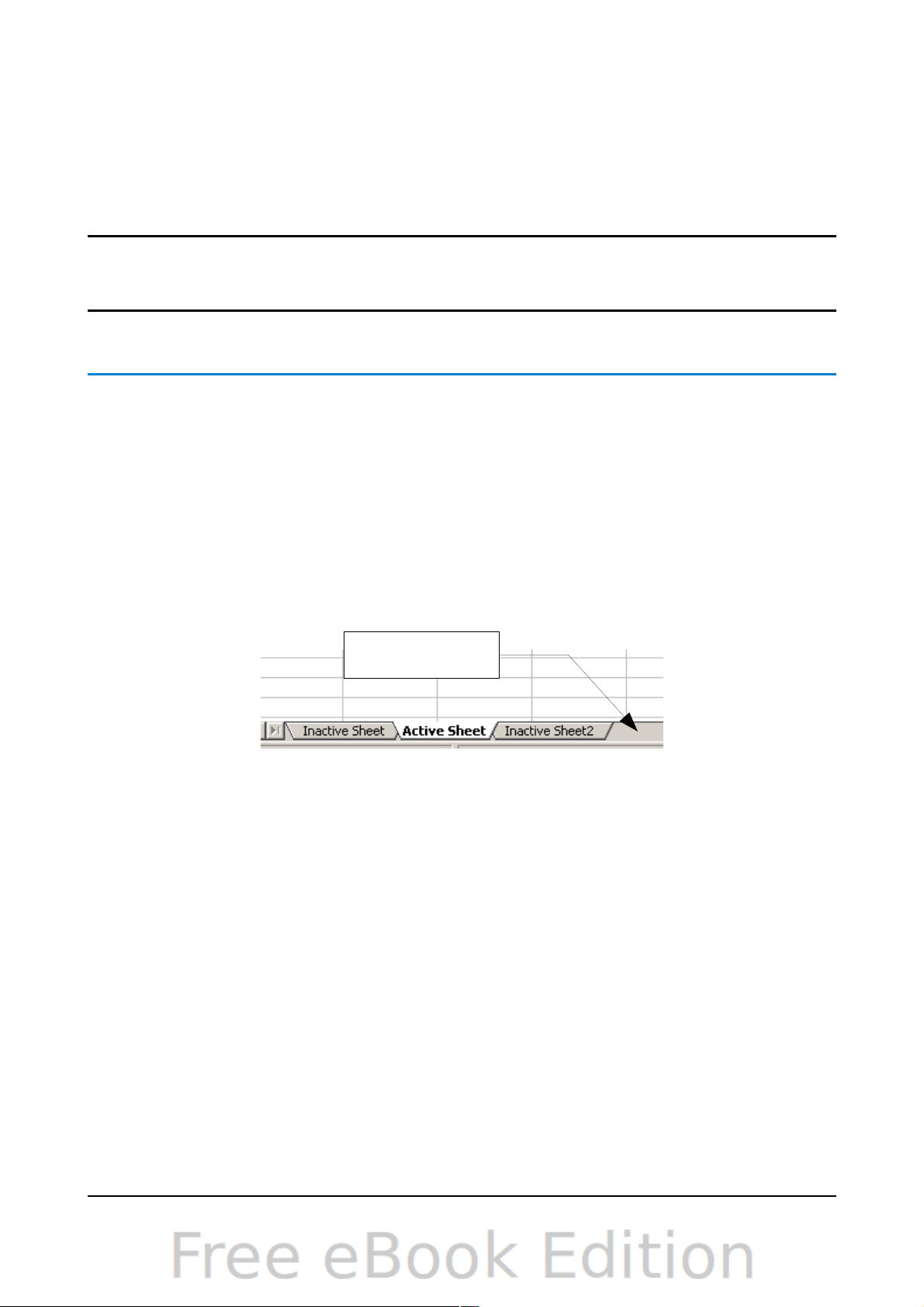
At the bottom of the grid of cells are the sheet tabs. These tabs enable access to each individual sheet, with the visible (active) sheet having a white tab. Clicking on another sheet tab displays that sheet, and its tab turns white. You can also select multiple sheet tabs at once by holding down the Control key while you click the names.

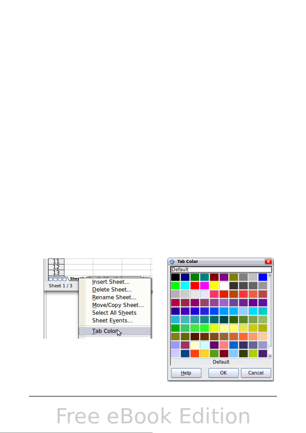
From Calc 3.3, you can choose colors for the different sheet tabs. Right-click on a tab and choose Tab Color from the pop-up menu to open a palette of colors. To add new colors to the palette, see “Color options” in Chapter 14 (Setting up and Customizing Calc).

16 OpenOffice.org 3.3 Calc Guide

Figure 10: Choose tab color

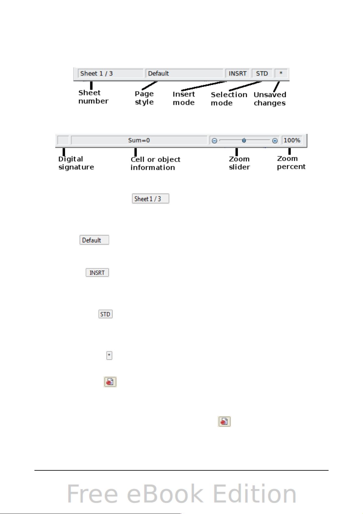
Status bar

The Calc status bar provides information about the spreadsheet and convenient ways to quickly change some of its features.

Sheet sequence number ( )

Shows the sequence number of the current sheet and the total number of sheets in the spreadsheet. The sequence number may not correspond with the name on the sheet tab.

Page style ( )

Shows the page style of the current sheet. To edit the page style, double-click on this field. The Page Style dialog opens.

Insert mode ( )

Click to toggle between INSRT (Insert) and OVER (Overwrite) modes when typing. This field is blank when the spreadsheet is not in a typing mode (for example, when selecting cells).

Selection mode ( )

Click to toggle between STD (Standard), EXT (Extend), and ADD (Add) selection. EXT is an alternative to Shift+click when selecting cells. See page 29 for more information.

Unsaved changes ( )

An asterisk (*) appears here if changes to the spreadsheet have not been saved.

Digital signature ( )

If the document has not been digitally signed, double-clicking in this area opens the Digital Signatures dialog, where you can sign the document. See Chapter 6 (Printing, Exporting, and E-mailing) for more about digital signatures.

If the document has been digitally signed, an icon shows in this area. You can double-click the icon to view the certificate. A document can be digitally signed only after it has been saved.

Chapter 1 Introducing Calc 17

Figure 11: Left end of Calc status bar

Figure 12: Right end of Calc status bar

Cell or object information ( )

Displays information about the selected items. When a group of cells is selected, the sum of the contents is displayed by default; you can right-click on this field and select other functions, such as the average value, maximum value, minimum value, or count (number of items selected).

When the cursor is on an object such as a picture or chart, the information shown includes the size of the object and its location.

Zoom ( )

To change the view magnification, drag the Zoom slider or click on the + and – signs. You can also right-click on the zoom level percentage to select a magnification value or double-click to open the Zoom & View Layout dialog.

Starting new spreadsheets

You can start a new, blank document in Calc in several ways.

• From the operating system menu, in the same way that you start other

programs. When OOo was installed on your computer, in most cases a menu entry for each component was added to your system menu. If you are using a Mac, you should see the OpenOffice.org icon in the Applications folder. When you double-click this icon, OOo opens at the Start Center (Figure 14).

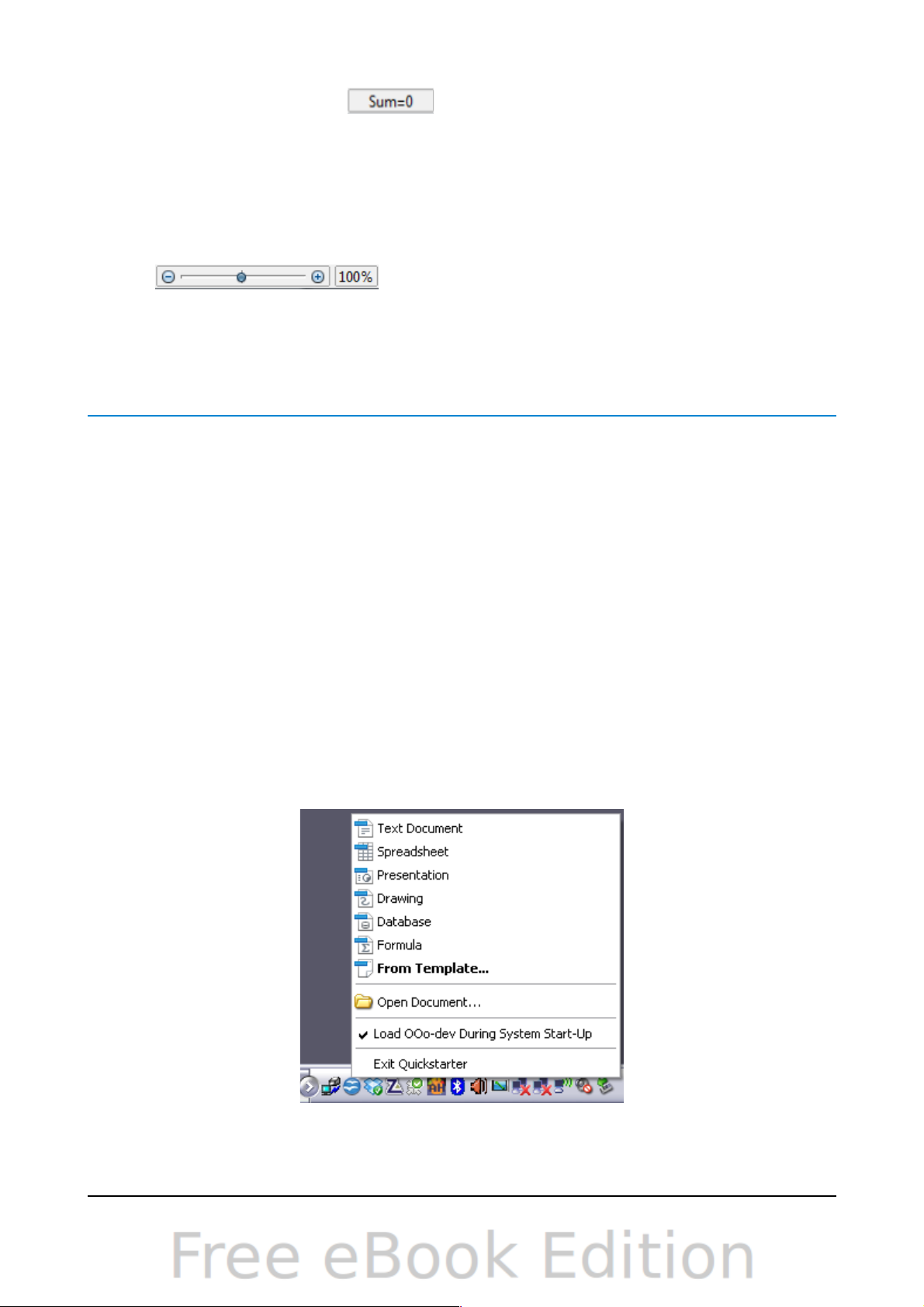
• From the Quickstarter, which is found in Windows, some Linux distributions,

and (in a slightly different form) in Mac OS X. The Quickstarter is an icon that is placed in the system tray or the dock during system startup. It indicates that OpenOffice.org has been loaded and is ready to use.

Right-click the Quickstarter icon (Figure 13) in the system tray to open a popup menu from which you can open a new document, open the Templates and Documents dialog box, or choose an existing document to open. You can also double-click the Quickstarter icon to display the Templates and Documents dialog box.

See Chapter 1 (Introducing OpenOffice.org) in the Getting Started guide for more information about using the Quickstarter.

18 OpenOffice.org 3.3 Calc Guide

Figure 13: Quickstarter pop-up menu on Windows XP

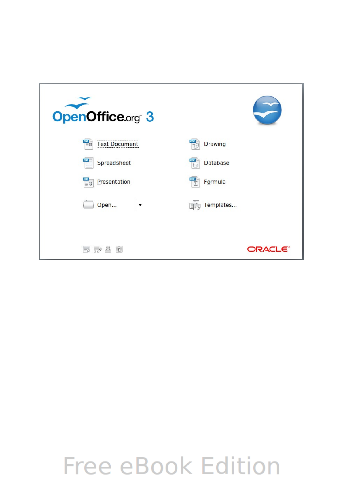
• From the Start Center. When OOo is open but no document is open (for

example, if you close all the open documents but leave the program running), the Start Center is shown. Click one of the icons to open a new document of that type, or click the Templates icon to start a new document using a template. If a document is already open in OOo, the new document opens in a new window.

When OOo is open, you can also start a new document in one of the following ways.

• Press the Control+N keys.

• Use File > New > Spreadsheet.

• Click the New button on the main toolbar.

Starting a new document from a template

Calc documents can also be created from templates. Follow the above procedures, but instead of choosing Spreadsheet, choose the Templates icon from the Start Center or File > New >Templates and Documents from the Menu bar or toolbar.

On the Templates and Documents window (Figure 15), navigate to the appropriate folder and double-click on the required template. A new spreadsheet, based on the selected template, opens.

A new OpenOffice.org installation does not contain many templates, but you can add more by downloading them from http://extensions.services.openoffice.org/ and installing them as described in Chapter 14 (Setting Up and Customizing Calc).

Chapter 1 Introducing Calc 19

Figure 14: OpenOffice.org Start Center

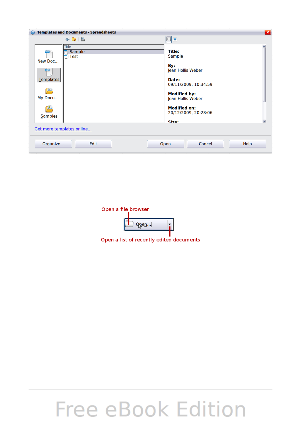
Figure 15: Starting a new spreadsheet from a template

Opening existing spreadsheets

When no document is open, the Start Center (Figure 14) provides an icon for opening an existing document or choosing from a list of recently-edited documents.

You can also open an existing document in one of the following ways. If a document is already open in OOo, the second document opens in a new window.

• Choose File > Open....

• Click the Open button on the main toolbar.

• Press Control+O on the keyboard.

• Use File > Recent Documents to display the last 10 files that were opened in

any of the OOo components.

• Use the Open Document or Recent Documents selections on the

Quickstarter.

In each case, the Open dialog box appears. Select the file you want, and then click Open. If a document is already open in OOo, the second document opens in a new window.

If you have associated Microsoft Office file formats with OpenOffice.org, you can also open these files by double-clicking on them.

20 OpenOffice.org 3.3 Calc Guide

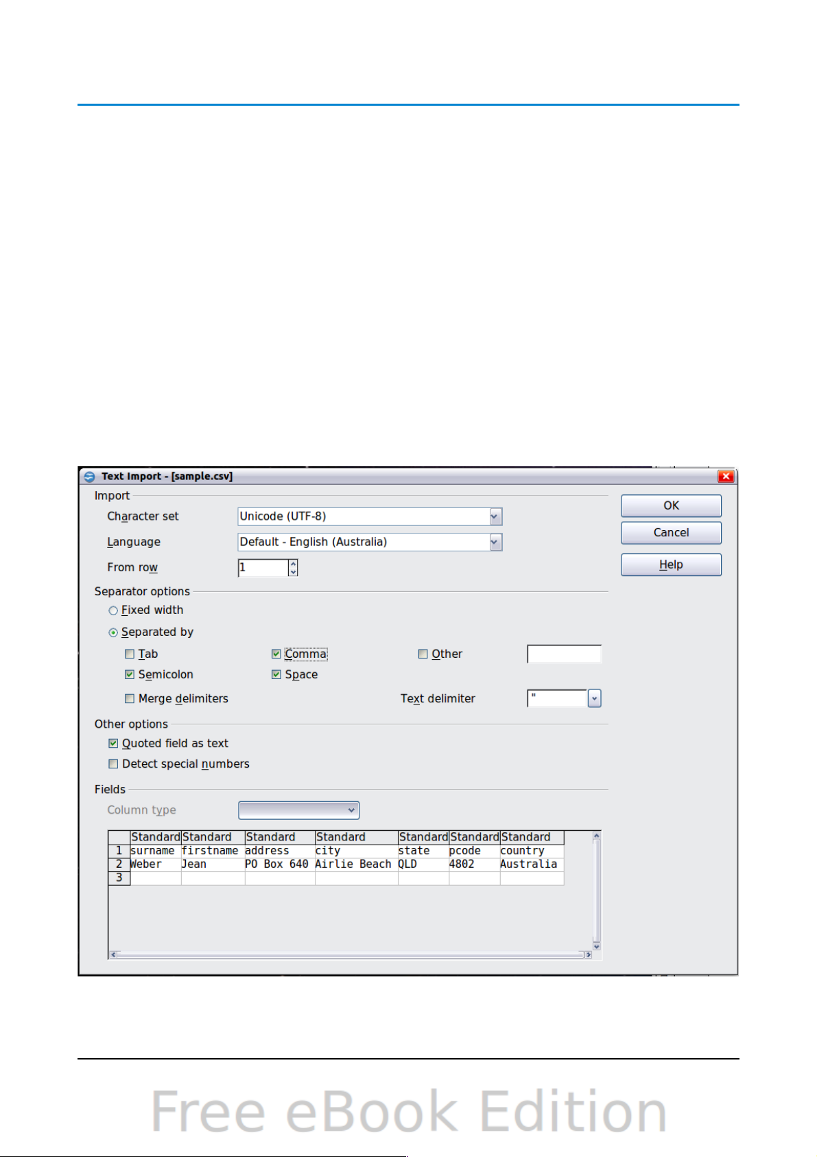
Opening CSV files

Comma-separated-values (CSV) files are text files that contain the cell contents of a single sheet. Each line in a CSV file represents a row in a spreadsheet. Commas, semicolons, or other characters are used to separate the cells. Text is entered in quotation marks; numbers are entered without quotation marks.

To open a CSV file in Calc:

1) Choose File > Open.

2) Locate the CSV file that you want to open.

3) If the file has a *.csv extension, select the file and click Open.

4) If the file has another extension (for example, *.txt), select the file, select Text CSV (*csv;*txt;*xls) in the File type box (scroll down into the spreadsheet section to find it) and then click Open.

5) On the Text Import dialog (Figure 16), select the Separator options to divide the text in the file into columns.

You can preview the layout of the imported data at the bottom of the dialog. Right-click a column in the preview to set the format or to hide the column.

If the CSV file uses a text delimiter character that is not in the Text delimiter list, click in the box, and type the character.

Chapter 1 Introducing Calc 21

Figure 16: Text Import dialog, with Comma (,) selected as the separator and double quotation mark (“) as the text delimiter.

6) In OOo 3.3, two new options are available when importing CSV files that contain data separated by specific characters.

These options determine whether quoted data will always be imported as text, and whether Calc will automatically detect all number formats, including special number formats such as dates, time, and scientific notation. The detection depends on the language settings.

7) Click OK to open the file.

Caution

If you do not select Text CSV (*csv;*txt;*xls) as the file type when opening the file, the document opens in Writer, not Calc.

Saving spreadsheets

Spreadsheets can be saved in three ways.

• Press Control+S.

• Choose File > Save (or Save All or Save As).

• Click the Save button on the main toolbar.

If the spreadsheet has not been saved previously, then each of these actions will open the Save As dialog. There you can specify the spreadsheet name and the location in which to save it.

Note

If the spreadsheet has been previously saved, then saving it using the Save (or Save All) command will overwrite an existing copy. However, you can save the spreadsheet in a different location or with a different name by selecting File > Save As.

Saving a document automatically

You can choose to have Calc save your spreadsheet automatically at regular intervals. Automatic saving, like manual saving, overwrites the last saved state of the file. To set up automatic file saving:

1) Choose Tools > Options > Load/Save > General.

2) Click on Save AutoRecovery information every and set the time interval. The default value is 15 minutes. Enter the value you want by typing it or by pressing the up or down arrow keys.

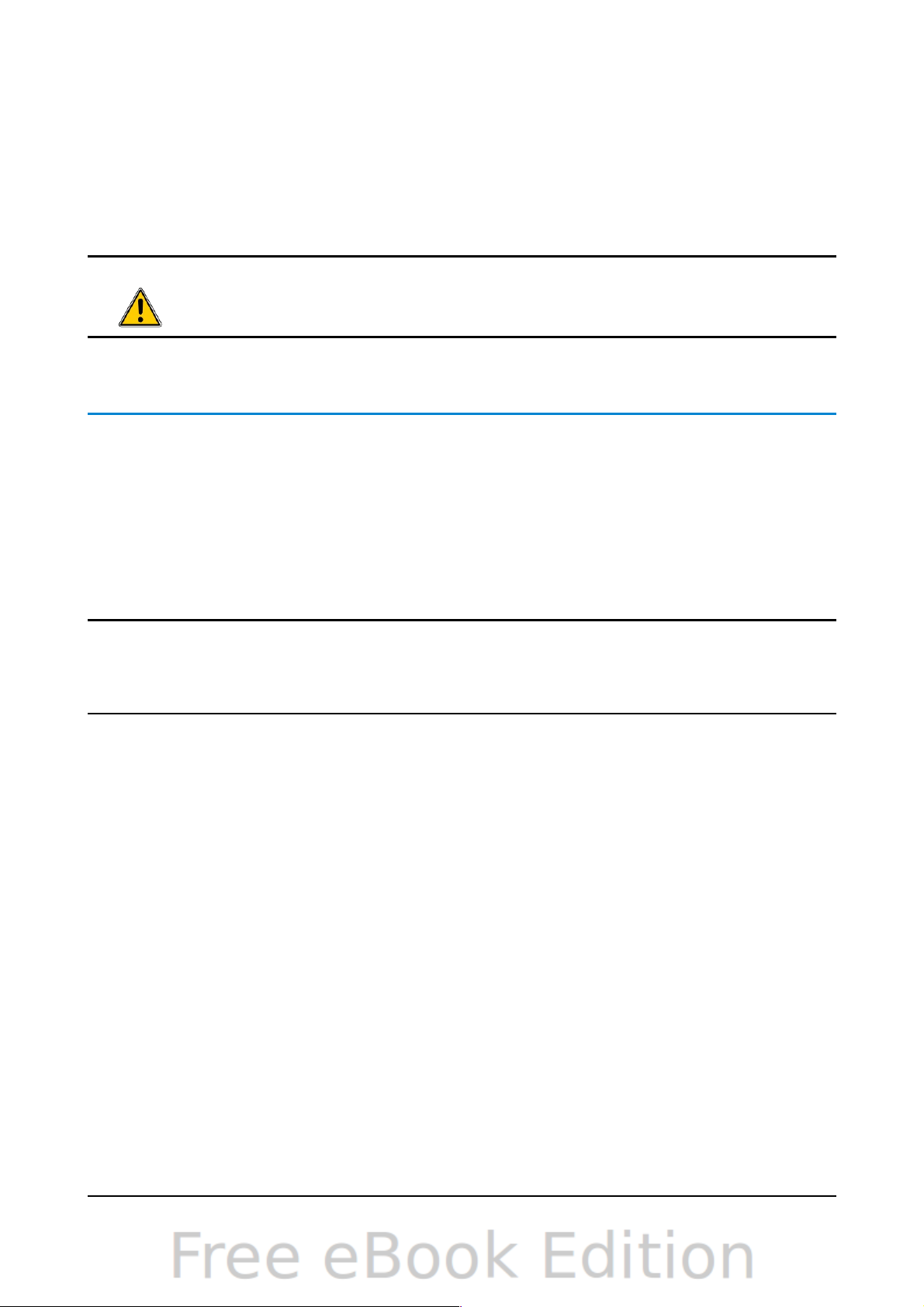
Saving as a Microsoft Excel document

If you need to exchange files with users of Microsoft Excel, they may not know how to open and save *.ods files. Only Microsoft Excel 2007 with Service Pack 2 (SP2) can do this. Users of Microsoft Excel 2007, 2003, XP, and 2000 can also download and install a free OpenDocument Format (ODF) plugin from Sun Microsystems, available from Softpedia, http://www.softpedia.com/get/Office-tools/Other-Office-Tools/Sun-ODF-

Plugin-for-Microsoft-Office.shtml.

22 OpenOffice.org 3.3 Calc Guide

Some users of Microsoft Excel may be unwilling or unable to receive *.ods files. (Perhaps their employer does not allow them to install the plug-in.) In this case, you can save a document as a Excel file (*.xls or *.xlsx).

1) Important—First save your spreadsheet in the file format used by OpenOffice.org, *.ods. If you do not, any changes you may have made since the last time you saved it will only appear in the Microsoft Excel version of the document.

2) Then choose File > Save As.

3) On the Save As dialog (Figure 17), in the File type (or Save as type) dropdown menu, select the type of Excel format you need. Click Save.

Caution

From this point on, all changes you make to the spreadsheet will occur only in the Microsoft Excel document. You have changed the name and

file type of your document. If you want to go back to working with the *.ods version of your spreadsheet, you must open it again.

Tip

To have Calc save documents by default in a Microsoft Excel file format, go to Tools > Options > Load/Save > General. In the section named Default file format and ODF settings, under Document type, select Spreadsheet, then under Always save as, select your preferred file format.

Chapter 1 Introducing Calc 23

Figure 17. Saving a spreadsheet in Microsoft Excel format

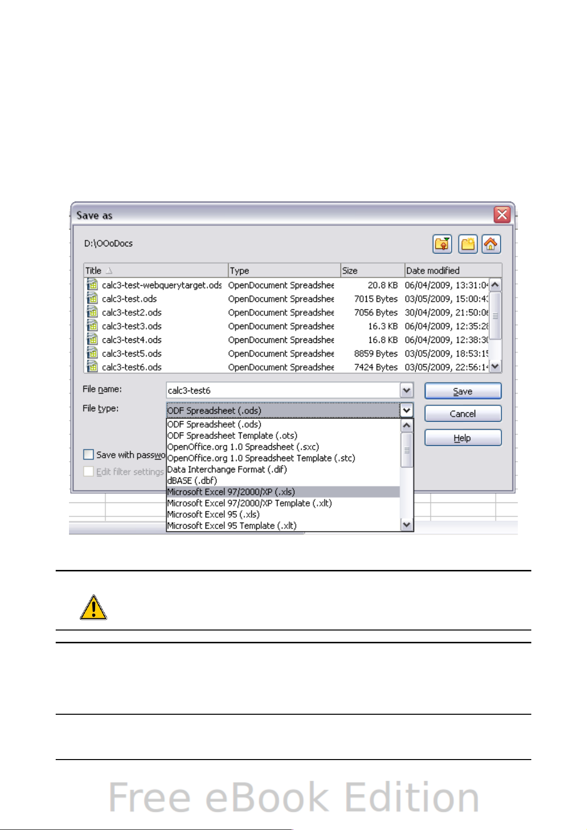
Saving as a CSV file

To save a spreadsheet as a comma separated value (CSV) file:

1) Choose File > Save As.

2) In the File name box, type a name for the file.

3) In the File type list, select Text CSV (*.csv;*.txt;*.xls) and click Save.

You may see the message box shown below. Click Keep Current Format.

4) In the Export of text files dialog, select the options you want and then click OK.

Saving in other formats

Calc can save spreadsheets in a range of formats, including HTML (Web pages), through the Save As dialog. Calc can also export spreadsheets to the PDF and XHTML file formats. See Chapter 6 (Printing, Exporting, and E-mailing) for more information.

Password protection

Calc provides two levels of document protection: read-protect (file cannot be viewed without a password) and write-protect (file can be viewed in read-only mode but cannot be changed without a password). Thus you can make the content available for reading by a selected group of people and for reading and editing by a different group. This behavior is compatible with Microsoft Excel file protection.

24 OpenOffice.org 3.3 Calc Guide

Figure 18: Choosing options when exporting to Text CSV

1) Use File > Save As when saving the document. (You can also use File > Save the first time you save a new document.)

2) On the Save As dialog, type the file name, select the Save with password option, and then click Save.

3) The Set Password dialog opens.

Here you have several choices:

• To read-protect the document, type a password in the two fields at the top

of the dialog box.

• To write-protect the document, click the More Options button and select

the Open file read-only checkbox.

Chapter 1 Introducing Calc 25

Figure 19: Two levels of password protection

• To write-protect the document but allow selected people to edit it, select

the Open file read-only checkbox and type a password in the two boxes at the bottom of the dialog box.

4) Click OK to save the file. If either pair of passwords do not match, you receive an error message. Close the message box to return to the Set Password dialog box and enter the password again.

Caution

OOo uses a very strong encryption mechanism that makes it almost impossible to recover the contents of a document if you lose the password.

Navigating within spreadsheets

Calc provides many ways to navigate within a spreadsheet from cell to cell and sheet to sheet. You can generally use whatever method you prefer.

Going to a particular cell

Using the mouse

Place the mouse pointer over the cell and click.

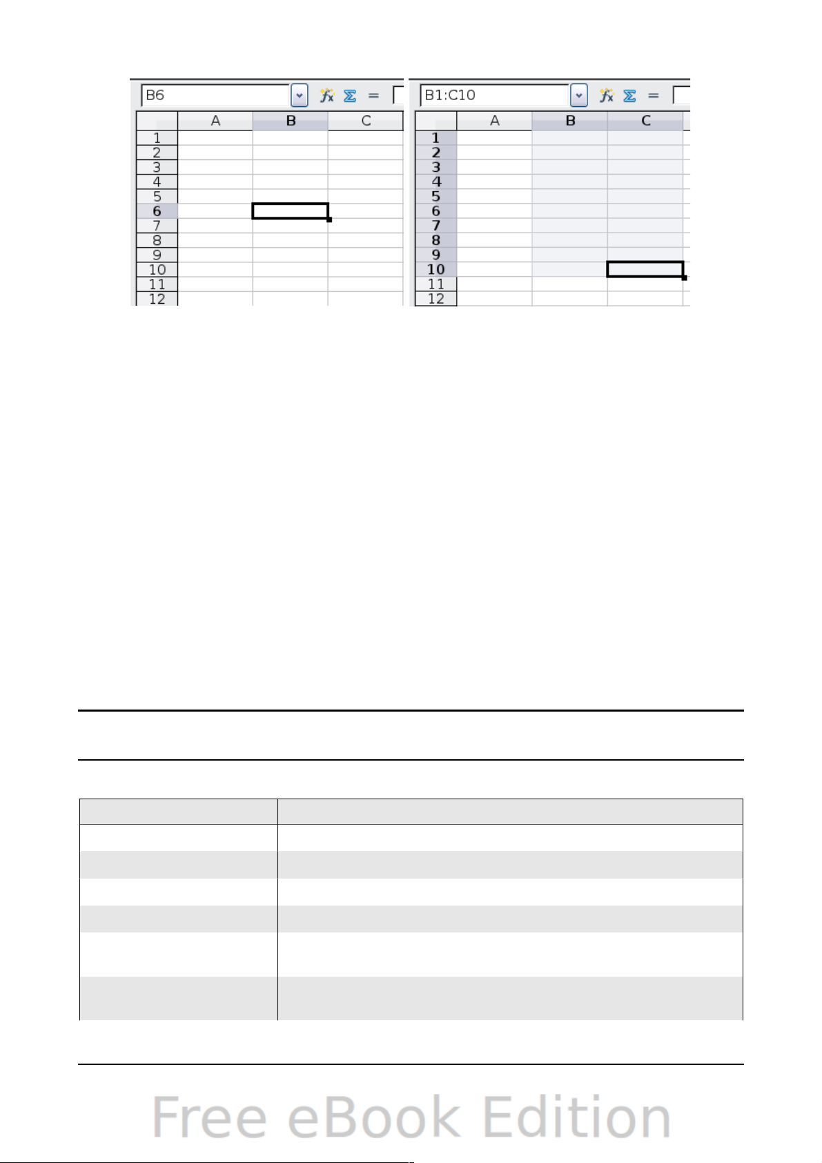
Using a cell reference

Click on the little inverted black triangle just to the right of the Name Box (Figure

9). The existing cell reference will be highlighted. Type the cell reference of the

cell you want to go to and press Enter. Cell references are case insensitive: a3 or A3, for example, are the same. Or just click into the Name Box, backspace over

the existing cell reference, and type in the cell reference you want and press Enter.

Using the Navigator

Click on the Navigator button in the Standard toolbar (or press F5) to display the Navigator. Type the cell reference into the top two fields, labeled Column and

Row, and press Enter. In Figure 32 on page 39, the Navigator would select cell A7. For more about using the Navigator, see page 38.

Moving from cell to cell

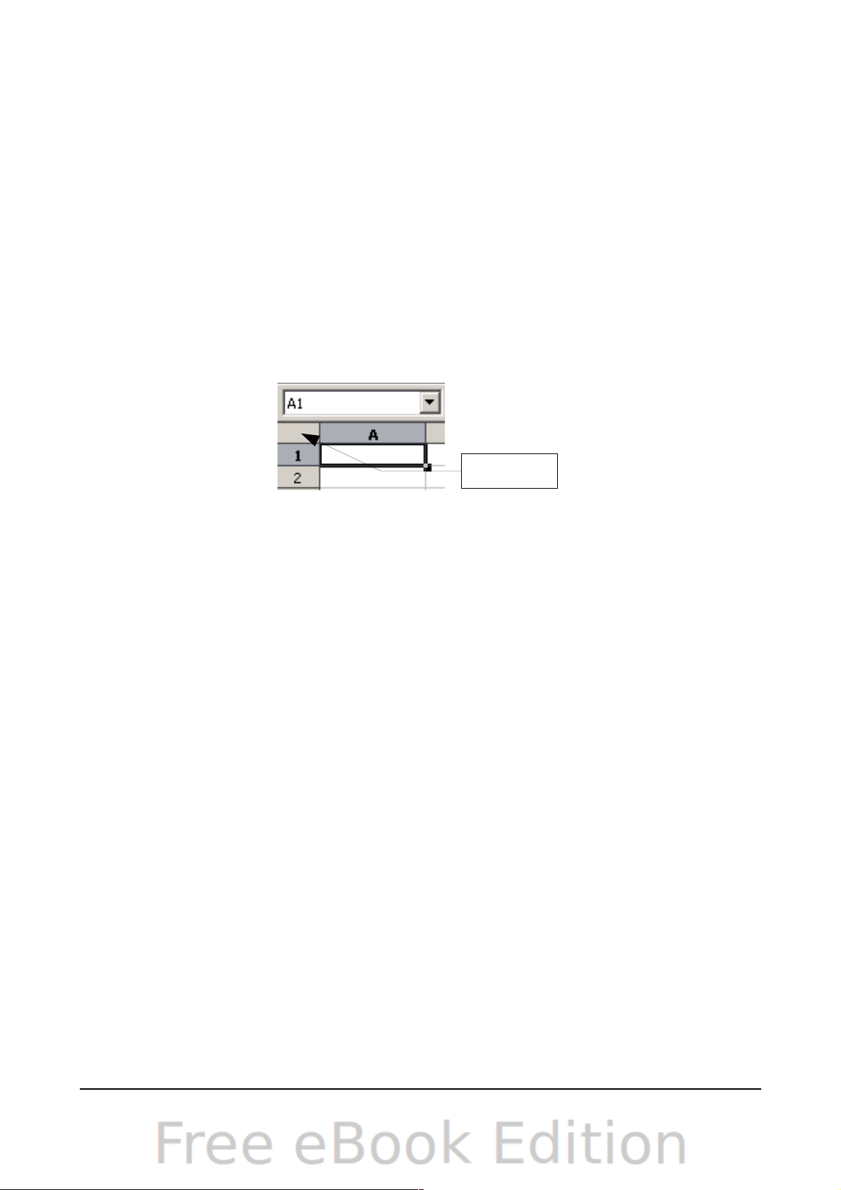
In the spreadsheet, one cell normally has a darker black border. This black border indicates where the focus is (see Figure 20). The focus indicates which cell is enabled to receive input. If a group of cells is selected, they have a highlight color (usually gray), with the focus cell having a dark border.

Using the mouse

To move the focus using the mouse, simply move the mouse pointer to the cell where you want the focus to be and click the left mouse button. This action changes the focus to the new cell. This method is most useful when the two cells are a large distance apart.

26 OpenOffice.org 3.3 Calc Guide

Using the Tab and Enter keys

• Pressing Enter or Shift+Enter moves the focus down or up, respectively.

• Pressing Tab or Shift+Tab moves the focus to the right or to the left,

respectively.

Using the arrow keys

Pressing the arrow keys on the keyboard moves the focus in the direction of the arrows.

Using Home, End, Page Up and Page Down

• Home moves the focus to the start of a row.

• End moves the focus to the column furthest to the right that contains data.

• Page Down moves the display down one complete screen and Page Up moves

the display up one complete screen.

• Combinations of Control (often represented on keyboards as Ctrl) and Alt with

Home, End, Page Down (PgDn), Page Up (PgUp), and the arrow keys move the focus of the current cell in other ways. Table 1 describes the keyboard

shortcuts for moving about a spreadsheet.

Tip

Use one of the four Alt+Arrow key combinations to resize the height or width of a cell. (For example: Alt+↓ increases the height of a cell.)

Table 1. Moving from cell to cell using the keyboard

Key Combination Movement

→

Right one cell

←

Left one cell

↑

Up one cell

↓

Down one cell

Control+→

To the next column to the right containing data in that row or to Column AMJ

Control+←

To the next column to the left containing data in that row or to Column A

Chapter 1 Introducing Calc 27

Figure 20. (left) One selected cell and (right) a group of selected cells

Key Combination Movement

Control+↑

To the next row above containing data in that column or to Row 1

Control+↓

To the next row below containing data in that column or to Row 65536

Control+Home To Cell A1

Control+End To lower right-hand corner of the rectangular area

containing data

Alt+Page Downn One screen to the right (if possible)

Alt+Page Up One screen to the left (if possible)

Control+Page Down One sheet to the right (in sheet tabs)

Control+Page Up One sheet to the left (in sheet tabs)

Tab To the next cell on the right

Shift+Tab To the next cell on the left

Enter Down one cell (unless changed by user)

Shift+Enter Up one cell (unless changed by user)

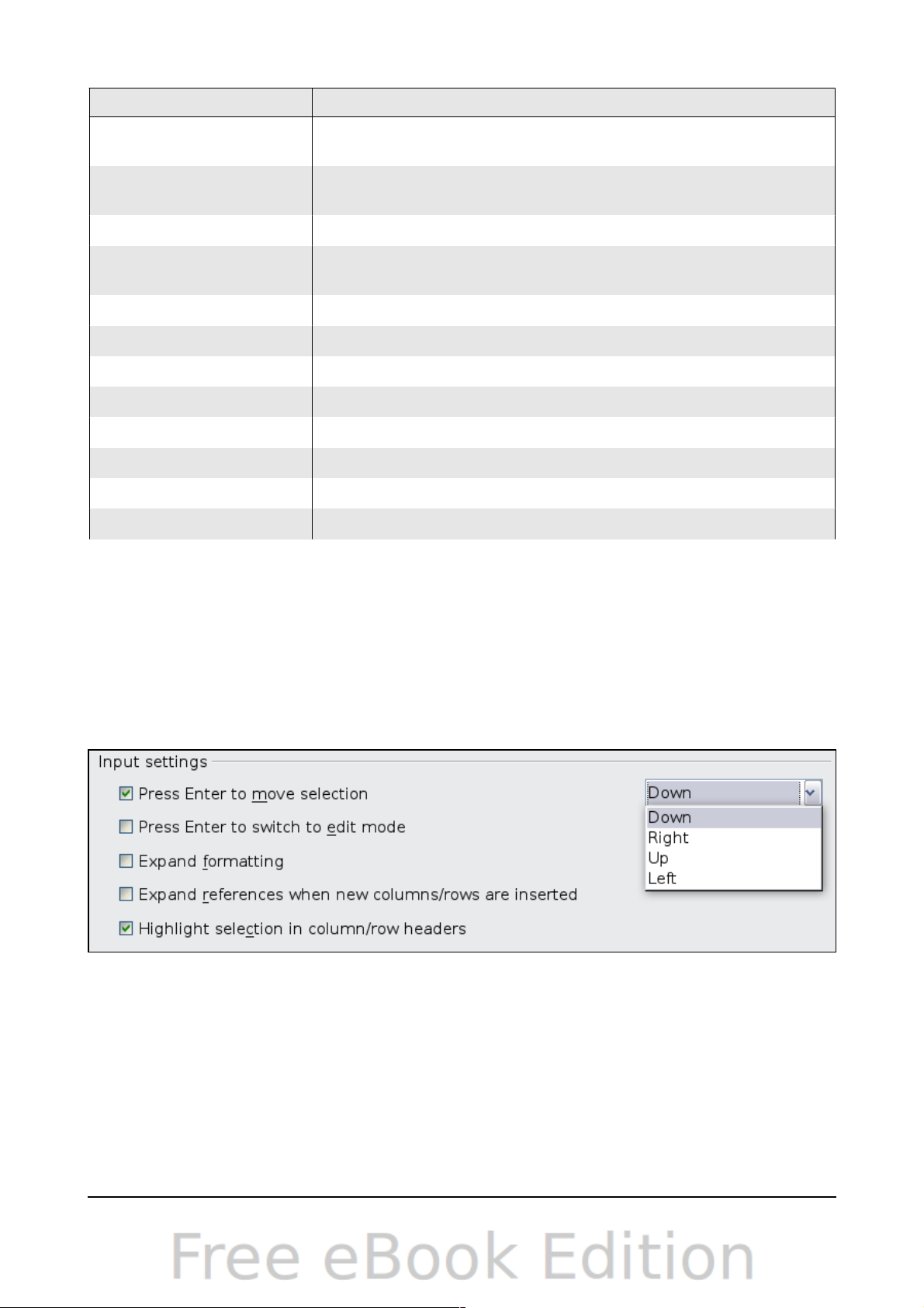
Customizing the effects of the Enter key

You can customize the direction in which the Enter key moves the focus, by selecting Tools > Options > OpenOffice.org Calc > General.

The four choices for the direction of the Enter key are shown on the right hand side of Figure 21. It can move the focus down, right, up, or left. Depending on the file being used or on the type of data being entered, setting a different direction can be useful.

The Enter key can also be used to switch into and out of the editing mode. Use the first two options under Input settings in Figure 21 to change the Enter key settings.

Moving from sheet to sheet

Each sheet in a spreadsheet is independent of the others, though they can be linked with references from one sheet to another. There are three ways to navigate between different sheets in a spreadsheet.

28 OpenOffice.org 3.3 Calc Guide

Figure 21: Customizing the effect of the Enter key

Using the keyboard

Pressing Control+Page Down moves one sheet to the right and pressing Control+Page Up moves one sheet to the left.

Using the mouse

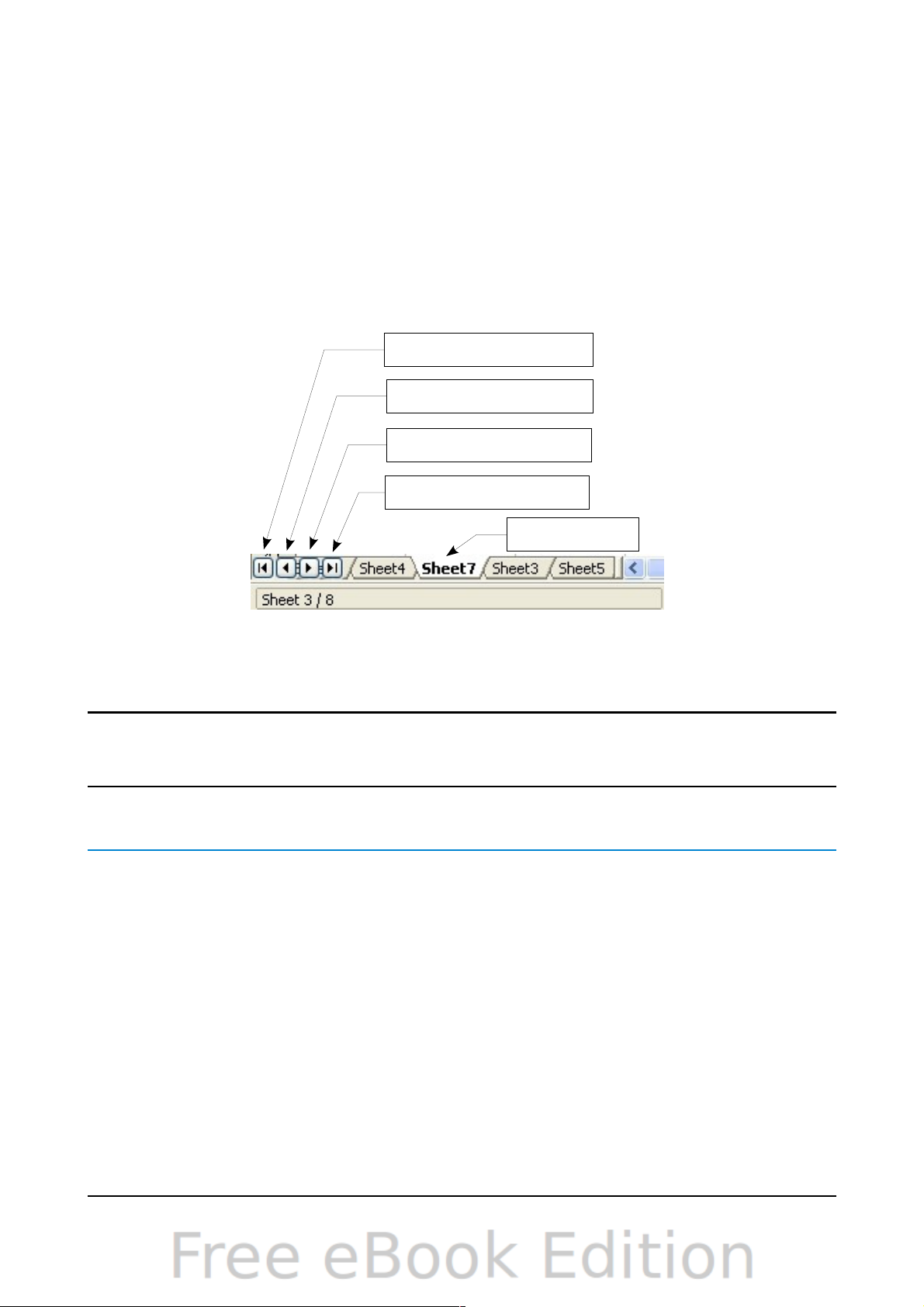
Clicking on one of the sheet tabs at the bottom of the spreadsheet selects that sheet.

If you have a lot of sheets, then some of the sheet tabs may be hidden behind the horizontal scroll bar at the bottom of the screen. If this is the case, then the four buttons at the left of the sheet tabs can move the tabs into view. Figure 22 shows how to do this.

Notice that the sheets here are not numbered in order. Sheet numbering is arbitrary; you can name a sheet as you wish.

Note

The sheet tab arrows that appear in Figure 22 only appear if you have some sheet tabs that can not be seen. Otherwise, they appear faded as in Figure 1.

Selecting items in a sheet or spreadsheet

Selecting cells

Cells can be selected in a variety of combinations and quantities.

Single cell

Left-click in the cell. The result will look like the left side of Figure 20. You can verify your selection by looking in the Name Box.

Range of contiguous cells

A range of cells can be selected using the keyboard or the mouse.

To select a range of cells by dragging the mouse:

1) Click in a cell.

2) Press and hold down the left mouse button.

Chapter 1 Introducing Calc 29

Move to the first sheet

Move left one sheet

Move right one sheet

Move to the last sheet

Sheet tabs

Figure 22. Sheet tab arrows

3) Move the mouse around the screen.

4) Once the desired block of cells is highlighted, release the left mouse button.

To select a range of cells without dragging the mouse:

1) Click in the cell which is to be one corner of the range of cells.

2) Move the mouse to the opposite corner of the range of cells.

3) Hold down the Shift key and click.

Tip

You can also select a contiguous range of cells by first clicking in the STD field on the status bar and changing it to EXT, before clicking in the opposite corner of the range of cells in step 3 above. If you use this method, be sure to change EXT back to STD or you may find yourself extending the selection unintentionally.

To select a range of cells without using the mouse:

1) Select the cell that will be one of the corners in the range of cells.

2) While holding down the Shift key, use the cursor arrows to select the rest of the range.

The result of any of these methods looks like the right side of Figure 20.

Tip

You can also directly select a range of cells using the Name Box. Click into the Name Box as described in “Using a cell reference” on page 26. To select a range of cells, enter the cell reference for the upper lefthand cell, followed by a colon (:), and then the lower right-hand cell reference. For example, to select the range that would go from A3 to C6, you would enter A3:C6.

Range of noncontiguous cells

1) Select the cell or range of cells using one of the methods above.

2) Move the mouse pointer to the start of the next range or single cell.

3) Hold down the Control key and click or click-and-drag to select another range of cells to add to the first range.

4) Repeat as necessary.

Tip

You can also select a noncontiguous range of cells by first clicking twice in the STD field on the status bar to change it to ADD, before clicking on a cell that you want to add to the range of cells in step 3 above. This method works best when adding single cells to a range. If you use this method, be sure to change ADD back to STD or you may find yourself adding more selections unintentionally.

Selecting columns and rows

Entire columns and rows can be selected very quickly in OOo.

Single column or row

To select a single column, click on the column identifier letter (see Figure 1).

To select a single row, click on the row identifier number.

30 OpenOffice.org 3.3 Calc Guide

Multiple columns or rows

To select multiple columns or rows that are contiguous:

1) Click on the first column or row in the group.

2) Hold down the Shift key.

3) Click the last column or row in the group.

To select multiple columns or rows that are not contiguous:

1) Click on the first column or row in the group.

2) Hold down the Control key.

3) Click on all of the subsequent columns or rows while holding down the Control key.

Entire sheet

To select the entire sheet, click on the small box between the A column header and the 1 row header.

You can also press Control+A to select the entire sheet.

Selecting sheets

You can select either one or multiple sheets. It can be advantageous to select multiple sheets at times when you want to make changes to many sheets at once.

Single sheet

Click on the sheet tab for the sheet you want to select. The active sheet becomes white (see Figure 22).

Multiple contiguous sheets

To select multiple contiguous sheets:

1) Click on the sheet tab for the first desired sheet.

2) Move the mouse pointer over the sheet tab for the last desired sheet.

3) Hold down the Shift key and click on the sheet tab.

All the tabs between these two sheets will turn white. Any actions that you perform will now affect all highlighted sheets.

Multiple noncontiguous sheets

To select multiple noncontiguous sheets:

1) Click on the sheet tab for the first desired sheet.

2) Move the mouse pointer over the sheet tab for the second desired sheet.

3) Hold down the Control key and click on the sheet tab.

4) Repeat as necessary.

The selected tabs will turn white. Any actions that you perform will now affect all highlighted sheets.

Chapter 1 Introducing Calc 31

Select All

Figure 23. Select All box

All sheets

Right-click any one of the sheet tabs and choose Select All Sheets from the pop-up menu.

Working with columns and rows

Inserting columns and rows

Columns and rows can be inserted individually or in groups.

Note

When you insert a single new column, it is inserted to the left of the highlighted column. When you insert a single new row, it is inserted above the highlighted row.

Cells in the new columns or rows are formatted like the corresponding cells in the column or row before (or to the left of) which the new column or row is inserted.

Single column or row

Using the Insert menu:

1) Select the cell, column, or row where you want the new column or row inserted.

2) Choose either Insert > Columns or Insert > Rows.

Using the mouse:

1) Select the cell, column, or row where you want the new column or row inserted.

2) Right-click the header of the column or row.

3) Choose Insert Rows or Insert Columns.

Multiple columns or rows

Multiple columns or rows can be inserted at once rather than inserting them one at a time.

1) Highlight the required number of columns or rows by holding down the left mouse button on the first one and then dragging across the required number of identifiers.

2) Proceed as for inserting a single column or row above.

Deleting columns and rows

Columns and rows can be deleted individually or in groups.

Single column or row

A single column or row can be deleted by using the mouse:

1) Select the column or row to be deleted.

2) Choose Edit > Delete Cells from the menu bar.

Or,

1) Right-click on the column or row header.

2) Choose Delete Columns or Delete Rows from the pop-up menu.

32 OpenOffice.org 3.3 Calc Guide

Multiple columns or rows

Multiple columns or rows can be deleted at once rather than deleting them one at a time.

1) Highlight the required columns or rows by holding down the left mouse button on the first one and then dragging across the required number of identifiers.

2) Proceed as for deleting a single column or row above.

Tip

Instead of deleting a row or column, you may wish to delete the contents of the cells but keep the empty row or column. See Chapter 2 (Entering, Editing, and Formatting Data) for instructions.

Working with sheets

Like any other Calc element, sheets can be inserted, deleted, and renamed.

Inserting new sheets

There are several ways to insert a new sheet. The first step for all of the methods is to select the sheets that the new sheet will be inserted next to. Then any of the following options can be used.

• Choose Insert > Sheet from the menu bar.

• Right-click on the sheet tab and choose Insert Sheet.

• Click in an empty space at the end of the line of sheet tabs.

Each method will open the Insert Sheet dialog (Figure 25). Here you can select whether the new sheet is to go before or after the selected sheet and how many sheets you want to insert. If you are inserting only one sheet, there is the opportunity to give the sheet a name.

Deleting sheets

Sheets can be deleted individually or in groups.

Single sheet

Right-click on the tab of the sheet you want to delete and choose Delete Sheet from the pop-up menu, or choose Edit > Sheet > Delete from the Menu bar. Either way, an alert will ask if you want to delete the sheet permanently. Click Yes.

Multiple sheets

To delete multiple sheets, select them as described earlier, then either right-click over one of the tabs and choose Delete Sheet from the pop-up menu, or choose Edit > Sheet > Delete from the Menu bar.

Chapter 1 Introducing Calc 33

Click here to insert a new sheet

Figure 24. Creating a new sheet

Figure 25: Insert Sheet dialog

Renaming sheets

The default name for the a new sheet is SheetX, where X is a number. While this works for a small spreadsheet with only a few sheets, it becomes awkward when there are many sheets.

To give a sheet a more meaningful name, you can:

• Enter the name in the Name box when you create the sheet, or

• Right-click on a sheet tab and choose Rename Sheet from the pop-up menu;

replace the existing name with a different one.

• (New in OOo3.1) Double-click on a sheet tab to pop up the Rename Sheet

dialog.

Note

Sheet names must start with either a letter or a number; other characters including spaces are not allowed. Apart from the first character of the sheet name, allowed characters are letters, numbers, spaces, and the underscore character. Attempting to rename a sheet with an invalid name will produce an error message.

Viewing Calc

Using Zoom

Use the zoom function to change the view to show more or fewer cells in the window.

In addition to using the Zoom slider (new in OOo 3.1) on the Status bar (see page 18), you can open the Zoom dialog and make a selection on the left-hand side.

• Choose View > Zoom from the Menu bar, or

• Double-click on the percentage figure in the Status bar at the bottom of the

window.

34 OpenOffice.org 3.3 Calc Guide

Figure 26. Zoom dialog

Optimal

Resizes the display to fit the width of the selected cells. To use this option, you must first highlight a range of cells.

Fit Width and Height

Displays the entire page on your screen.

Fit Width

Displays the complete width of the document page. The top and bottom edges of the page may not be visible.

100%

Displays the document at its actual size.

Variable

Enter a zoom percentage of your choice.

Freezing rows and columns

Freezing locks a number of rows at the top of a spreadsheet or a number of columns on the left of a spreadsheet or both. Then when scrolling around within the sheet, any

frozen columns and rows remain in view.

Figure 27 shows some frozen rows and columns. The heavier horizontal line between rows 3 and 14 and the heavier vertical line between columns C and H denote the

frozen areas. Rows 4 through 13 and columns D through G have been scrolled off the page. The first three rows and columns remained because they are frozen into place.

You can set the freeze point at one row, one column, or both a row and a column as in Figure 27.

Freezing single rows or columns

1) Click on the header for the row below where you want the freeze or for the column to the right of where you want the freeze.

2) Choose Window > Freeze. A dark line appears, indicating where the freeze is put.

Chapter 1 Introducing Calc 35

Figure 27. Frozen rows and columns

Freezing a row and a column

1) Click into the cell that is immediately below the row you want frozen and immediately to the right of the column you want frozen.

2) Choose Window > Freeze. Two lines appear on the screen, a horizontal line above this cell and a vertical

line to the left of this cell. Now as you scroll around the screen, everything above and to the left of these lines will remain in view.

Unfreezing

To unfreeze rows or columns, choose Window > Freeze. The check mark by Freeze will vanish.

Splitting the screen

Another way to change the view is by splitting the window, also known as splitting the screen. The

screen can be split horizontally, vertically, or both. You can therefore have up to four portions of the spreadsheet in view at any one time.

Why would you want to do this? An example would be a large spreadsheet in which one of the cells has a number in it that is used by three formulas in other cells. Using the split-screen technique, you can position the cell containing the number in one section and each of the cells with formulas in the other sections. Then you can change the number in the cell and watch how it affects each of the formulas.

36 OpenOffice.org 3.3 Calc Guide

Figure 28. Split screen example

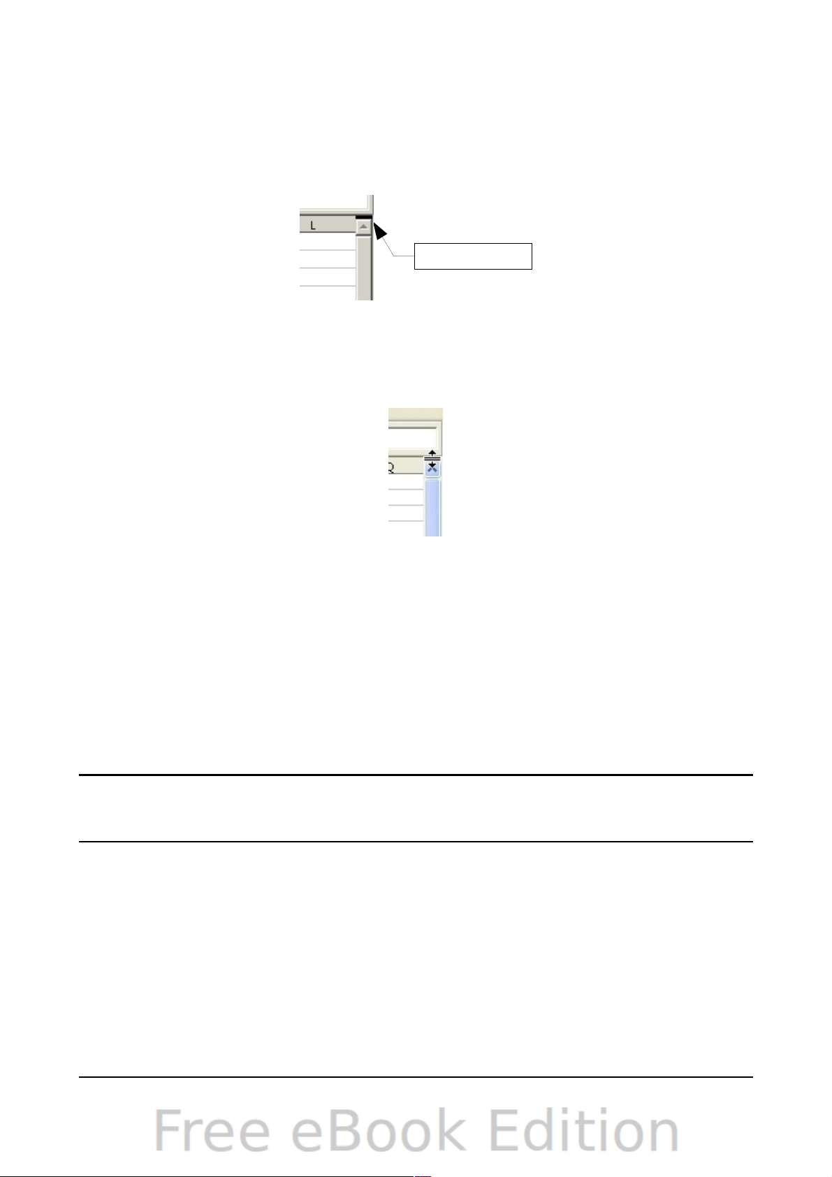
Splitting the screen horizontally

To split the screen horizontally:

1) Move the mouse pointer into the vertical scroll bar, on the right-hand side of the screen, and place it over the small button at the top with the black triangle.

2) Immediately above this button, you will see a thick black line (Figure 29). Move the mouse pointer over this line, and it turns into a line with two arrows (Figure 30).

3) Hold down the left mouse button. A gray line appears, running across the page. Drag the mouse downwards and this line follows.

4) Release the mouse button and the screen splits into two views, each with its own vertical scroll bar. You can scroll the upper and lower parts independently.

Notice in Figure 28, the Beta and the A0 values are in the upper part of the window and other calculations are in the lower part. Thus, you can make changes to the Beta

and A0 values and watch their effects on the calculations in the lower half of the window.

Tip

You can also split the screen using a menu command. Click in a cell immediately below and to the right of where you wish the screen to be split, and choose Window > Split.

Splitting the screen vertically

To split the screen vertically:

1) Move the mouse pointer into the horizontal scroll bar at the bottom of the screen and place it over the small button on the right with the black triangle.

Chapter 1 Introducing Calc 37

Split screen bar

Figure 29. Split screen bar on vertical scroll bar

Figure 30. Split-screen bar on vertical scroll bar with cursor

2) Immediately to the right of this button is a thick black line (Figure 31). Move the mouse pointer over this line and it turns into a line with two arrows.

3) Hold down the left mouse button, and a gray line appears, running up the page. Drag the mouse to the left and this line follows.

4) Release the mouse button, and the screen is split into two views, each with its own horizontal scroll bar. You can scroll the left and right parts of the window independently.

Removing split views

To remove a split view, do any of the following:

• Double-click on each split line.

• Click on and drag the split lines back to their places at the ends of the scroll

bars.

• Choose Window > Split to remove all split lines at the same time.

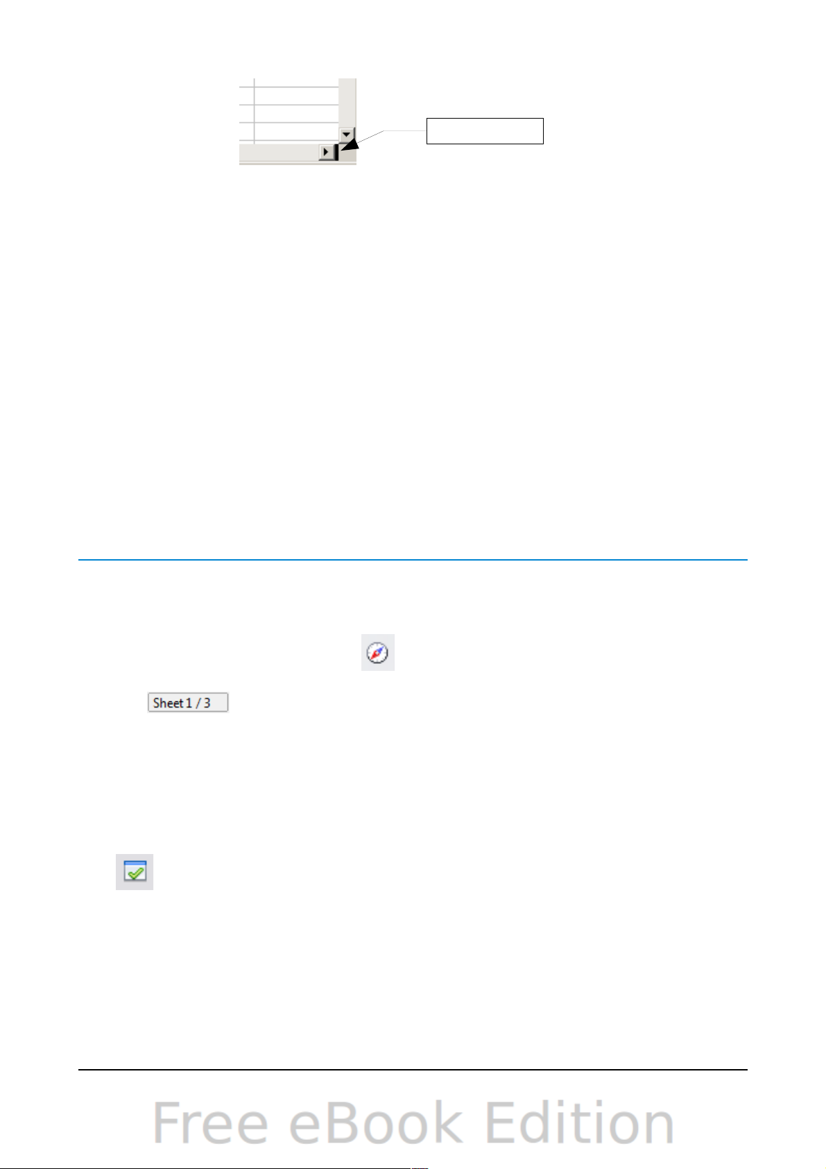
Using the Navigator

In addition to the cell reference boxes (labeled Column and Row), the Navigator provides several other ways to move quickly through a spreadsheet and find specific items.

To open the Navigator, click its icon on the Standard toolbar, or press F5, or choose View > Navigator on the Menu bar, or double-click on the Sheet Sequence

Number in the Status Bar. You can dock the Navigator to either side of the main Calc window or leave it floating. (To dock or float the Navigator, hold down the Control key and double-click in an empty area near the icons at the top.)

The Navigator displays lists of all the objects in a spreadsheet document, grouped into categories. If an indicator (plus sign or arrow) appears next to a category, at least one object of this kind exists. To open a category and see the list of items, click on the indicator.

To hide the list of categories and show only the icons at the top, click the Contents

icon . Click this icon again to show the list.

Table 2 summarizes the functions of the icons at the top of the Navigator.

38 OpenOffice.org 3.3 Calc Guide

Split screen bar

Figure 31: Split bar on horizontal scroll bar

Figure 32: The Navigator in Calc

Table 2: Function of icons in the Navigator

Icon Action

Data Range. Specifies the current data range denoted by the position of the cell cursor.

Start/End. Moves to the cell at the beginning or end of the current data range, which you can highlight using the Data Range button.

Contents. Shows or hides the list of categories.

Toggle. Switches between showing all categories and showing only the selected category.

Displays all available scenarios. Double-click a name to apply that scenario. See Chapter 9 (Data Analysis) for more information.

Drag Mode. Choose hyperlink, link, or copy. See “Choosing a drag mode” for details.

Moving quickly through a document

The Navigator provides several convenient ways to move around a document and find items in it:

• To jump to a specific cell in the current sheet, type its cell reference in the

Column and Row boxes at the top of the Navigator and press the Enter key; for example, in Figure 32 the cell reference is A7.

• When a category is showing the list of objects in it, double-click on an object to

jump directly to that object’s location in the document.

• To see the content in only one category, highlight that category and click the

Toggle icon. Click the icon again to display all the categories.

Chapter 1 Introducing Calc 39

• Use the Start and End icons to jump to the first or last cell in the selected

data range.

Tip

Ranges, scenarios, pictures, and other objects are much easier to find if you have given them informative names when creating them, instead of keeping Calc’s default Graphics 1, Graphics 2, Object 1, and so on, which may not correspond to the position of the object in the document.

Choosing a drag mode

Sets the drag and drop options for inserting items into a document using the Navigator.

Insert as Hyperlink

Creates a hyperlink when you drag and drop an item into the current document.

Insert as Link

Inserts the selected item as a link where you drag and drop an object into the current document.

Insert as Copy

Inserts a copy of the selected item where you drag and drop in the current document. You cannot drag and drop copies of graphics, OLE objects, or indexes.

Using document properties

To open the Properties dialog for a document, choose File > Properties.

The Properties dialog has six tabs. The information on the General page and the Statistics page is generated by the program. Other information (the name of the person on the Created and Modified lines of the General page) is derived from the User Data page in Tools > Options.

The Internet page is relevant only to HTML documents. The file sharing options on the Security page are discussed elsewhere in this book.

Use the Description and Custom Properties pages to hold:

• Metadata to assist in classifying, sorting, storing, and retrieving documents.

Some of this metadata is exported to the closest equivalent in HTML and PDF; some fields have no equivalent and are not exported.

• Information that changes. You can store data for use in fields in your

document; for example, the title of the document, contact information for a project participant, or the name of a product might change during the course of a project.

This dialog can be used in a template, where the field names can serve as reminders to users of information they need to include.

You can return to this dialog at any time and change the information you entered. When you do so, all of the references to that information will change wherever they appear in the document. For example, on the Description page (Figure 33) you might need to change the contents of the Title field from the draft title to the final title.

40 OpenOffice.org 3.3 Calc Guide

Figure 33: The Description page of the document’s Properties dialog

Use the Custom Properties page (Figure 34) to store information that does not fit into the fields supplied on the other pages of this dialog box.

When the Custom Properties page is first opened in a new document, it may be blank. However, if the new document is based on a template, this page may contain fields.

Click Add to insert a row of boxes into which you can enter your custom properties.

• The Name box includes a drop-down list of typical choices; scroll down to see

all the choices. If none of the choices meet your needs, you can type a new name into the box.

• In the Type column, you can choose from text, date+time, date, number,

duration, or yes/no for each field. You cannot create new types.

Chapter 1 Introducing Calc 41

Figure 34: Custom Properties page, showing drop-down lists of names and types

• In the Value column, type or select what you want to appear in the document

where this field is used. Choices may be limited to specific data types depending on the selection in the Type column; for example, if the Type selection is Date, the Value for that property is limited to a date.

To remove a custom property, click the button at the end of the row.

Tip

To change the format of the Date value, go to Tools > Options > Languages and change the Locale setting. Be careful! This change

affects all open documents, not just the current one.

42 OpenOffice.org 3.3 Calc Guide

Chapter 2

Entering, Editing, and

Formatting Data

Introduction

You can enter data into Calc in several ways: using the keyboard, the mouse (dragging and dropping), the Fill tool, and selection lists. Calc also provides the ability to enter information into multiple sheets of the same document at the same time.

After entering data, you can format and display it in various ways.

Entering data using the keyboard

Most data entry in Calc can be accomplished using the keyboard.

Entering numbers

Click in the cell and type in the number using the number keys on either the main keyboard or the numeric keypad.

To enter a negative number, either type a minus (–) sign in front of it or enclose it in parentheses (brackets), like this: (1234).

By default, numbers are right-aligned and negative numbers have a leading minus symbol.

Entering text

Click in the cell and type the text. Text is left-aligned by default.

Entering numbers as text

If a number is entered in the format 01481, Calc will drop the leading 0. (Exception: see Tip below.) To preserve the leading zero, for example for telephone area codes, type an apostrophe before the number, like this: '01481.

The data is now treated as text and displayed exactly as entered. Typically, formulas will treat the entry as a zero and functions will ignore it.

Tip

Numbers can have leading zeros and still be regarded as numbers (as opposed to text) if the cell is formatted appropriately. Right-click on the cell and chose Format Cells > Numbers. Adjust the Leading zeros setting to add leading zeros to numbers.

Note

When a plain apostrophe is used to allow a leading 0 to be displayed, it is not visible in the cell after the Enter key is pressed. If “smart quotes” are used for apostrophes, the apostrophe remains visible in the cell.

To choose this type of apostrophe, use Tools > AutoCorrect Options > Localized Options. Select the Replace option for apostrophes to activate this function. The selection of the apostrophe type affects both Calc and Writer.

44 OpenOffice.org 3.3 Calc Guide

Caution

When a number is formatted as text, take care that the cell containing the number is not used in a formula because Calc will ignore the value.

Entering dates and times

Select the cell and type the date or time. You can separate the date elements with a slash (/) or a hyphen (–) or use text such as 10 Oct 03. Calc recognizes a variety of

date formats. You can separate time elements with colons such as 10:43:45.

Entering special characters

A “special” character is one not found on a standard English keyboard. For example, © ¾ æ ç ñ ö ø ¢ are all special characters. To insert a special character:

1) Place the cursor in your document where you want the character to appear.

2) Click Insert > Special Character to open the Special Characters dialog (Figure 35).

3) Select the characters (from any font or mixture of fonts) you wish to insert, in order; then click OK. The selected characters are shown in the bottom left of the dialog. As you select each character, it is shown alone at the bottom right, along with the numerical code for that character.

Note

Different fonts include different special characters. If you do not find a particular special character you want, try changing the Font selection.

Inserting dashes

To enter en and em dashes, you can use the Replace dashes option under Tools > AutoCorrect Options > Options tab. This option replaces two hyphens, under

certain conditions, with the corresponding dash.

In the following table, the A and B represent text consisting of letters A to z or digits 0 to 9.

Chapter 2 Entering, Editing, and Formatting Data 45

Figure 35: The Special Characters dialog

Text that you type: Result

A - B (A, space, minus, space, B) A – B (A, space, en-dash, space, B)

A -- B (A, space, minus, minus, space, B) A – B (A, space, en-dash, space, B)

A--B (A, minus, minus, B) A—B (A, em-dash, B)

A-B (A, minus, B) A-B (unchanged)

A -B (A, space, minus, B) A -B (unchanged)

A --B (A, space, minus, minus, B) A –B (A, space, en-dash, B)

Deactivating automatic changes

Calc automatically applies many changes during data input, unless you deactivate those changes. You can also immediately undo any automatic changes with Ctrl+Z.

AutoCorrect changes

Automatic correction of typing errors, replacement of straight quotation marks by curly (custom) quotes, and starting cell content with an uppercase (capital) letter are controlled by Tools > AutoCorrect Options. Go to the Options or Replace tabs to deactivate any of the features that you do not want. On the Replace tab, you can also delete unwanted word pairs and add new ones as required.

AutoInput

When you are typing in a cell, Calc automatically suggests matching input found in the same column. To turn the AutoInput on and off, set or remove the check mark in front of Tools > Cell Contents > AutoInput.

Automatic date conversion

Calc automatically converts certain entries to dates. To ensure that an entry that looks like a date is interpreted as text, type an apostrophe at the beginning of the entry. The apostrophe is not displayed in the cell.

Speeding up data entry

Entering data into a spreadsheet can be very labor-intensive, but Calc provides several tools for removing some of the drudgery from input.

The most basic ability is to drop and drag the contents of one cell to another with a mouse. Many people also find AutoInput helpful. Calc also includes several other tools for automating input, especially of repetitive material. They include the Fill tool, selection lists, and the ability to input information into multiple sheets of the same document.

Using the Fill tool on cells

At its simplest, the Fill tool is a way to duplicate existing content. Start by selecting the cell to copy, then drag the mouse in any direction (or hold down the Shift key and click in the last cell you want to fill), and then choose Edit > Fill and the direction in which you want to copy: Up, Down, Left or Right.

46 OpenOffice.org 3.3 Calc Guide

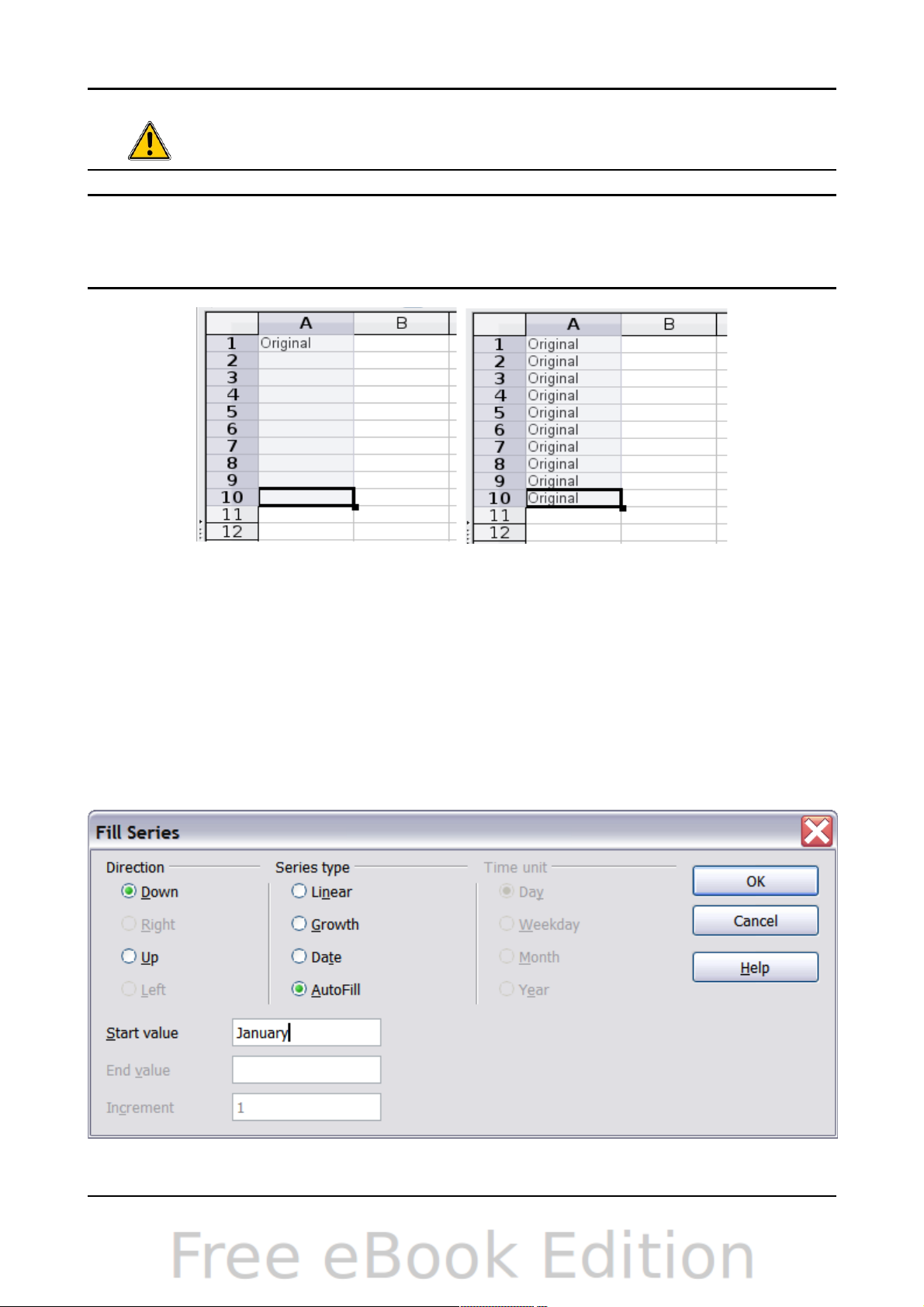
Caution

Choices that are not available are grayed out, but you can still choose the opposite direction from what you intend, which could cause you to overwrite cells accidentally.

Tip

A shortcut way to fill cells is to grab the “handle” in the lower righthand corner of the cell and drag it in the direction you want to fill. If the cell contains a number, the number will fill in series. If the cell contains text, the same text will fill in the direction you chose.

Using a fill series

A more complex use of the Fill tool is to use a fill series. The default lists are for the full and abbreviated days of the week and the months of the year, but you can create your own lists as well.

To add a fill series to a spreadsheet, select the cells to fill, choose Edit > Fill >

Series. In the Fill Series dialog, select AutoFill as the Series type, and enter as the Start value an item from any defined series. The selected cells then fill in the other

items on the list sequentially, repeating from the top of the list when they reach the end of the list.

Chapter 2 Entering, Editing, and Formatting Data 47

Figure 36: Using the Fill tool

Figure 37: Specifying the start of a fill series (result is in Figure 38)

Figure 38: Result of fill series

You can also use Edit > Fill > Series to create a one-time fill series for numbers by entering the start and end values and the increment. For example, if you entered start and end values of 1 and 7 with an increment of 2, you would get the sequence of 1, 3, 5, 7.

In all these cases, the Fill tool creates only a momentary connection between the cells. Once they are filled, the cells have no further connection with one another.

Defining a fill series

To define your own fill series, go to Tools > Options > OpenOffice.org Calc > Sort Lists. This dialog shows the previously-defined series in the Lists box on the left, and

the contents of the highlighted list in the Entries box.

Click New. The Entries box is cleared. Type the series for the new list in the Entries box (one entry per line), and then click Add.

48 OpenOffice.org 3.3 Calc Guide

selection shown in Figure 37

Figure 39: Predefined fill series

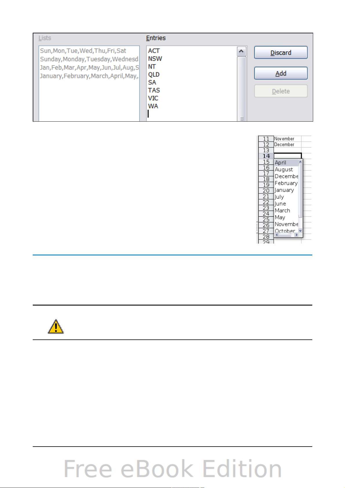
Figure 40: Defining a new fill series

Using selection lists

Selection lists are available only for text, and are limited to using only text that has already been entered in the same column.

To use a selection list, select a blank cell and press Ctrl+D. A drop-down list appears on any cell in the same column that either has at least one text character or whose format is defined as text. Click on the entry you require.

Sharing content between sheets

You might want to enter the same information in the same cell on multiple sheets, for example to set up standard listings for a group of individuals or organizations. Instead of entering the list on each sheet individually, you can enter it in all the sheets at once. To do this, select all the sheets (Edit > Sheet > Select), then enter the information in the current one.

Caution

This technique overwrites any information that is already in the cells on the other sheets—without any warning. For this reason, when you are finished, be sure to deselect all the sheets except the one you want to edit. (Ctrl+click on a sheet tab to select or deselect the sheet.)

Chapter 2 Entering, Editing, and Formatting Data 49

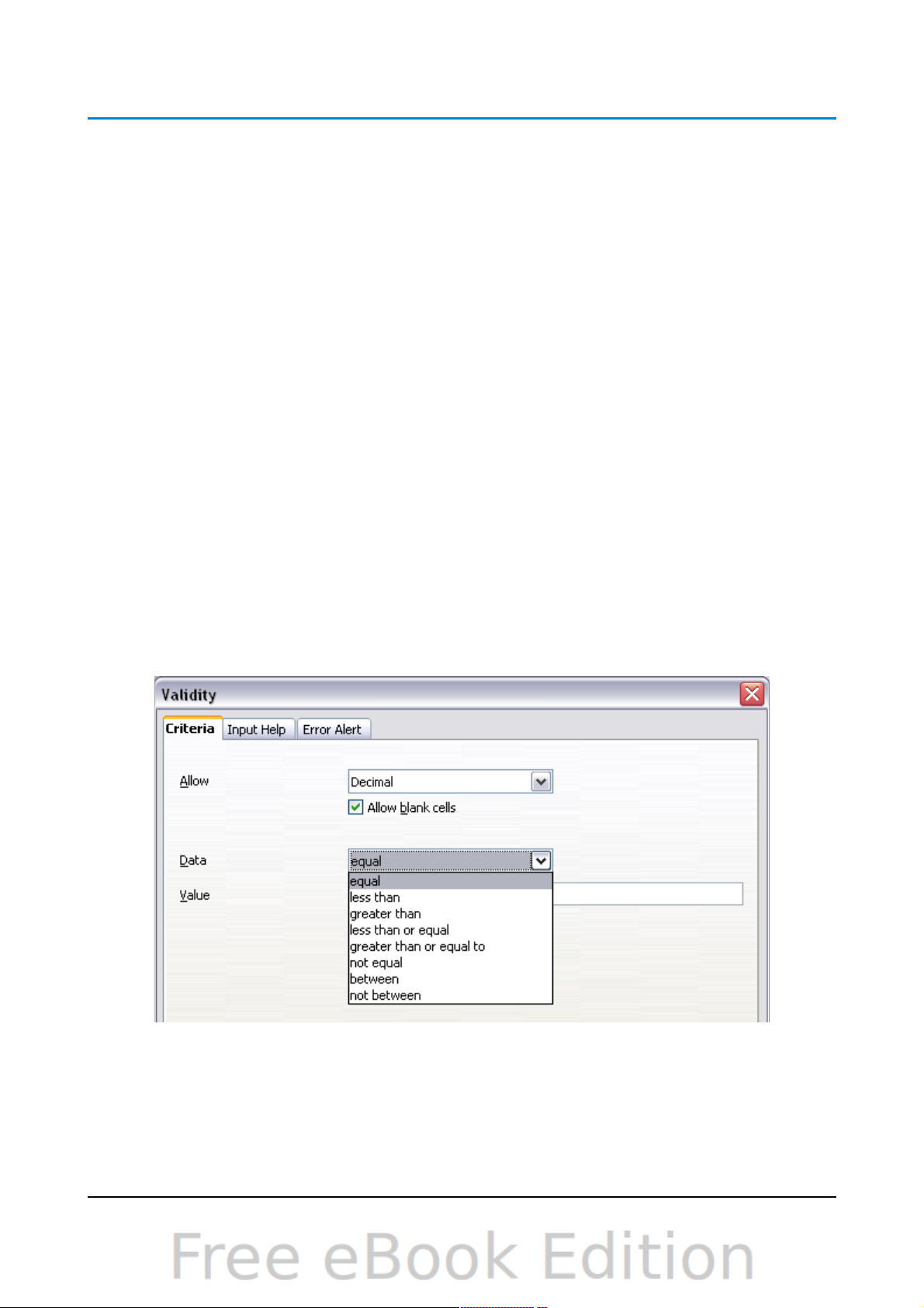
Validating cell contents

When creating spreadsheets for other people to use, you may want to make sure they enter data that is valid or appropriate for the cell. You can also use validation in your own work as a guide to entering data that is either complex or rarely used.

Fill series and selection lists can handle some types of data, but they are limited to predefined information. To validate new data entered by a user, select a cell and use Data > Validity to define the type of contents that can be entered in that cell. For example, a cell might require a date or a whole number, with no alphabetic characters or decimal points; or a cell may not be left empty.

Depending on how validation is set up, the tool can also define the range of values that can be entered and provide help messages that explain the content rules you have set up for the cell and what users should do when they enter invalid content. You can also set the cell to refuse invalid content, accept it with a warning, or—if you are especially well-organized—start a macro when an error is entered.

Validation is most useful for cells containing functions. If cells are set to accept invalid content with a warning, rather than refusing it, you can use Tools > Detective > Mark Invalid Data to find the cells with invalid data. The Detective function marks any cells containing invalid data with a circle.

Note that a validity rule is considered part of a cell’s format. If you select Format or Delete All from the Delete Contents window, then it is removed. (Repeating the Detective’s Mark Invalid Data command removes the invalid data circle, because the data is no longer invalid.) If you want to copy a validity rule with the rest of the cell, use Edit > Paste Special > Paste Formats or Paste All.

Figure 41 shows the choices for a typical validity test. Note the Allow blank cells option under the Allow list.

The validity test options vary with the type of data selected from the Allow list. For example, Figure 42 shows the choices when a cell must contain a cell range.

50 OpenOffice.org 3.3 Calc Guide

Figure 41: Typical validity test choices

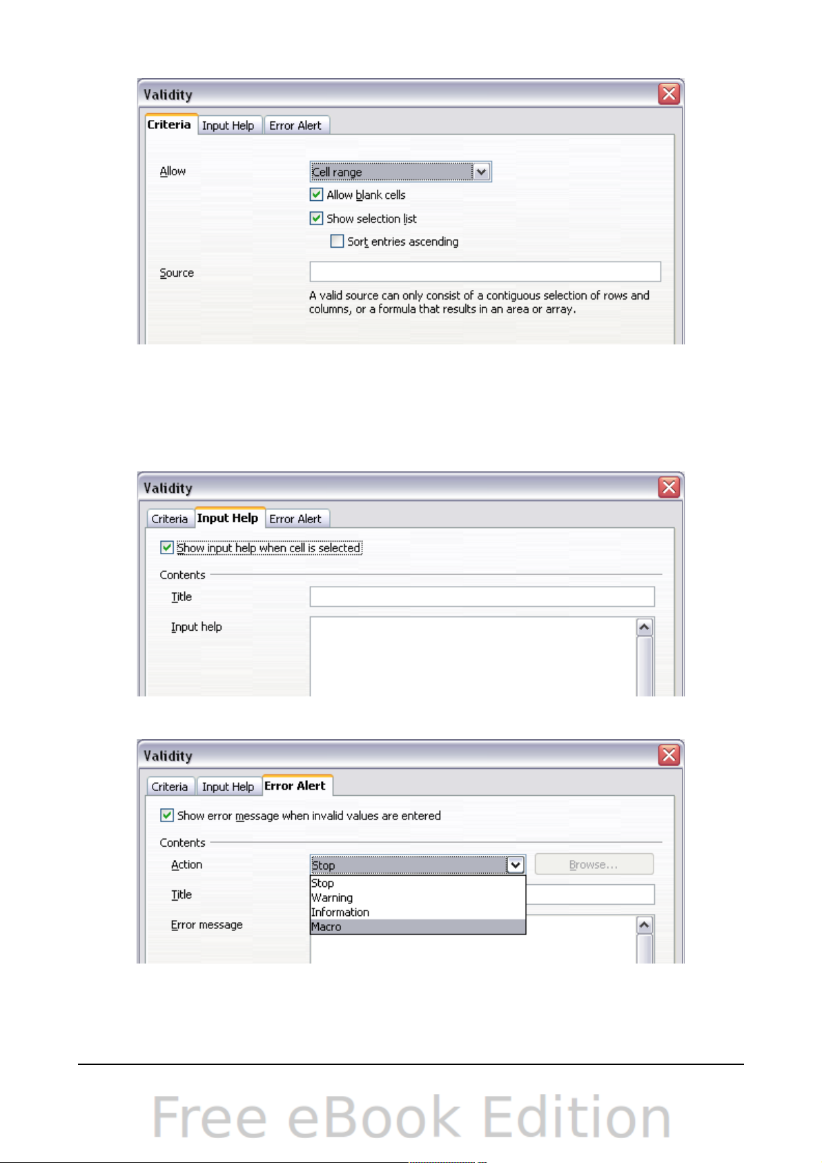
Figure 42: Validity choices for a cell range

To provide input help for a cell, use the Input Help page of the Validity dialog (Figure

43). To show an error message when an invalid value is entered, use the Error Alert page (Figure 44). Be sure to write something helpful, explaining what a valid entry should contain—not just “Invalid data—try again” or something similar.

Chapter 2 Entering, Editing, and Formatting Data 51

Figure 43: Defining input help for a cell

Figure 44: Defining an error message for a cell with invalid data

Editing data

Editing data is done is in much the same way as entering it. The first step is to select the cell containing the data to be edited.

Removing data from a cell

Data can be removed (deleted) from a cell in several ways.

Removing data only

The data alone can be removed from a cell without removing any of the formatting of the cell. Click in the cell to select it, and then press the Backspace key.

Removing data and formatting

The data and the formatting can be removed from a cell at the same time. Press the Delete key (or right-click and choose Delete Contents, or use Edit > Delete Contents) to open the Delete Contents dialog (Figure 45). From this dialog, different aspects of the cell can be deleted. To delete everything in a cell (contents and format), check Delete all.

Replacing all the data in a cell

To remove data and insert new data, simply type over the old data. The new data will retain the original formatting.

Changing part of the data in a cell

Sometimes it is necessary to change the contents of a cell without removing all of the contents, for example when the phrase “See Dick run” is in a cell and it needs to be changed to “See Dick run fast.” It is often useful to do this without deleting the old cell contents first.

The process is the similar to the one described above, but you need to place the cursor inside the cell. You can do this in two ways.

52 OpenOffice.org 3.3 Calc Guide

Figure 45: Delete Contents dialog

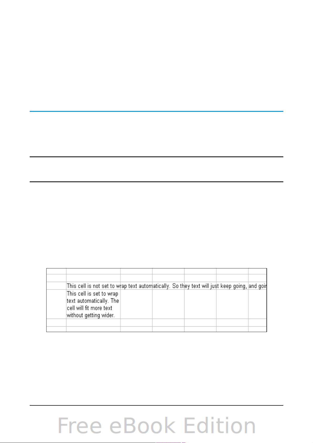
Using the keyboard

After selecting the appropriate cell, press the F2 key and the cursor is placed at the end of the cell. Then use the keyboard arrow keys to move the cursor through the text in the cell.

Using the mouse

Using the mouse, either double-click on the appropriate cell (to select it and place the cursor in it for editing), or single-click to select the cell and then move the mouse pointer up to the input line and click into it to place the cursor for editing.

Formatting data

The data in Calc can be formatted in several ways. It can either be edited as part of a cell style so that it is automatically applied, or it can be applied manually to the cell. Some manual formatting can be applied using toolbar icons. For more control and extra options, select the appropriate cell or cells range, right-click on it, and select Format Cells. All of the format options are discussed below.

Note

All the settings discussed in this section can also be set as a part of the cell style. See Chapter 4 (Using Styles and Templates) for more information.

Formatting multiple lines of text

Multiple lines of text can be entered into a single cell using automatic wrapping or manual line breaks. Each method is useful for different situations.

Using automatic wrapping

To set text to wrap at the end of the cell, right-click on the cell and select Format Cells (or choose Format > Cells from the menu bar, or press Ctrl+1). On the

Alignment tab (Figure 47), under Properties, select Wrap text automatically. The results are shown below (Figure 46).

Chapter 2 Entering, Editing, and Formatting Data 53

Figure 46: Automatic text wrap

Figure 47: Format Cells > Alignment dialog

Using manual line breaks

To insert a manual line break while typing in a cell, press Ctrl+Enter. This method does not work with the cursor in the input line. When editing text, first double-click the cell, then single-click at the position where you want the line break.

When a manual line break is entered, the cell width does not change. Figure 48 shows the results of using two manual line breaks after the first line of text.

Shrinking text to fit the cell

The font size of the data in a cell can automatically adjust to fit in a cell. To do this, select the Shrink to fit cell option in the Format Cells dialog (Figure 47). Figure 49 shows the results.

54 OpenOffice.org 3.3 Calc Guide

Figure 48: Cell with manual line breaks

Figure 49: Shrinking font size to fit cells

Formatting numbers

Several different number formats can be applied to cells by using icons on the Formatting toolbar. Select the cell, then click the relevant icon. Some icons may not be visible in a default setup; click the down-arrow at the end of the Formatting bar and select other icons to display.

In OOo 3.3, numbers formatted with the General number format will display as many decimal digits as required. In former versions of OOo, a maximum of 2 decimal digits were displayed with the General number format.

For more control or to select other number formats, use the Numbers tab (Figure 51) of the Format Cells dialog.

• Apply any of the data types in the Category list to the data.

• Control the number of decimal places and leading zeros.

• Enter a custom format code.

The Language setting controls the local settings for the different formats such as the date order and the currency marker.

Chapter 2 Entering, Editing, and Formatting Data 55

Figure 50: Number format icons. Left to right: currency, percentage, date, exponential, standard, add decimal place, delete decimal place.

Figure 51: Format Cells > Numbers

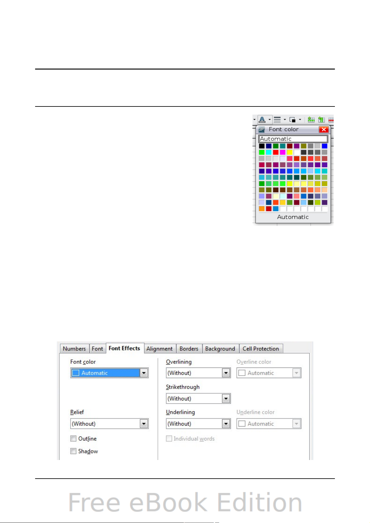
Formatting the font

To quickly choose the font used in a cell, select the cell, then click the arrow next to the Font Name box on the Formatting toolbar and choose a font from the list.

Tip

To choose whether to show the font names in their font or in plain text, go to Tools > Options > OpenOffice.org > View and select or deselect the Show preview of fonts option in the Font Lists section. For more information, see Chapter 14 (Setting Up and Customizing Calc).

To choose the size of the font, click the arrow next to the Font Size box on the Formatting toolbar. For other formatting, you can use the Bold, Italic, or Underline icons.

To choose a font color, click the arrow next to the Font Color icon to display a color palette. Click on the required color.

(To define custom colors, use Tools > Options > OpenOffice.org > Colors. See Chapter 14 for more information.)

To specify the language of the cell (useful because it allows different languages to exist in the same document and be spell checked correctly), use the Font tab of the Format Cells dialog. See Chapter 4 for more information.

Choosing font effects

The Font Effects tab (Figure 52) of the Format Cells dialog offers more font options.

Overlining and underlining

You can choose from a variety of overlining and underlining options (solid lines, dots, short and long dashes, in various combinations) and the color of the line.

Strikethrough

The strikethrough options include lines, slashes, and Xs.

Relief

The relief options are embossed (raised text), engraved (sunken text), outline, and shadow.

56 OpenOffice.org 3.3 Calc Guide

Figure 52: Format Cells > Font Effects

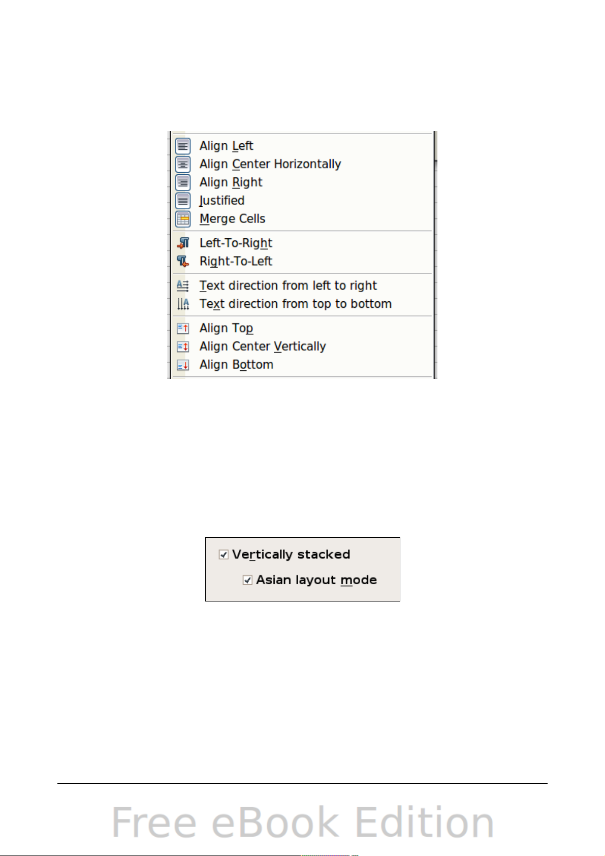
Setting cell alignment and orientation

Some of the cell alignment and orientation icons are not shown by default on the Formatting toolbar. To show them, click on the small arrow at the right-hand end of the toolbar and select them from the list of icons.

Some of the alignment and orientation icons are available only if you have Asian or CTL (Complex Text Layout) languages enabled (in Tools > Options > Language Settings > Languages). If you choose an unavailable icon from the list, it does not appear on the toolbar.

For more control and other choices, use the Alignment tab (Figure 47) of the Format Cells dialog to set the horizontal and vertical alignment and rotate the text. If you have Asian languages enabled, then the Text orientation section shows an extra option (labeled Asian layout mode) under the Vertically stacked option, as shown in Figure 54.

The difference in results between having Asian layout mode on or off is shown in Figure 55.

Chapter 2 Entering, Editing, and Formatting Data 57

Figure 53: Cell alignment and orientation

Figure 54: Asian layout mode option

Figure 55: Types of vertical stacking

Formatting the cell borders

To quickly choose a line style and color for the borders of a cell, click the small arrows next to the Line Style and Line Color icons on the Formatting toolbar. If the Line Style and Line Color icons are not displayed in the formatting toolbar, select

the down arrow on the right side of the bar, then select Visible Buttons. In each case, a palette of choices is displayed.

For more control, including the spacing between the cell borders and the text, use the Borders tab of the Format Cells dialog. There you can also define a shadow. See Chapter 4 for details.

Note

The cell border properties apply to a cell, and can only be changed if you are editing that cell. For example, if cell C3 has a top border (which would be equivalent visually to a bottom border on C2), that border can only be removed by selecting C3. It cannot be removed in C2.

Formatting the cell background

To quickly choose a background color for a cell, click the small arrow next to the Background Color icon on the Formatting toolbar. A palette of color choices, similar to the Font Color palette, is displayed.

(To define custom colors, use Tools > Options > OpenOffice.org > Colors. See Chapter 14 for more information.)

You can also use the Background tab of the Format Cells dialog. See Chapter 4 for details.

58 OpenOffice.org 3.3 Calc Guide

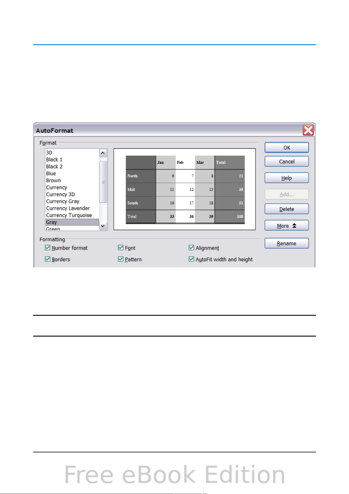
Autoformatting cells and sheets

You can use the AutoFormat feature to quickly apply a set of cell formats to a sheet or a selected cell range.

1) Select the cells that you want to format, including the column and row headers.

2) Choose Format > AutoFormat.

3) To select which properties (number format, font, alignment, borders, pattern, autofit width and height) to include in an AutoFormat, click More. Select or deselect the required options. Click OK.

If you do not see any change in color of the cell contents, choose View > Value Highlighting from the menu bar. This function only affects cells with numerical data.

Note

If the selected cell range does not have column and row headers, AutoFormat is not available.

Defining a new AutoFormat

You can define a new AutoFormat that is available to all spreadsheets.

1) Format a sheet.

2) Choose Edit > Select All.

3) Choose Format > AutoFormat. The Add button is now active.

4) Click Add.

5) In the Name box of the Add AutoFormat dialog, type a meaningful name for the new format.

6) Click OK to save. The new format is now available in the Format list in the AutoFormat dialog.

Chapter 2 Entering, Editing, and Formatting Data 59

Figure 56: Choosing an AutoFormat

Formatting spreadsheets using themes

Calc comes with a predefined set of formatting themes that you can apply to your spreadsheets.

It is not possible to add themes to Calc, and they cannot be modified. However, you can modify their styles after you apply them to a spreadsheet.

To apply a theme to a spreadsheet:

1) Click the Choose Themes icon in the Tools toolbar. If this toolbar is not visible, you can show it using View > Toolbars > Tools. The Theme Selection dialog appears. This dialog lists the available themes for the whole spreadsheet.

2) In the Theme Selection dialog, select the theme that you want to apply to the spreadsheet. As soon as you select a theme, some of the properties of the custom styles are applied to the open spreadsheet and are immediately visible.

3) Click OK. If you wish, you can now go to the Styles and Formatting window to modify specific styles. These modifications do not change the theme; they only change the appearance of this specific spreadsheet document.

Using conditional formatting

You can set up cell formats to change depending on conditions that you specify. For example, in a table of numbers, you can show all the values above the average in green and all those below the average in red.

Note

To apply conditional formatting, AutoCalculate must be enabled. Choose Tools > Cell Contents > AutoCalculate.

Conditional formatting depends upon the use of styles. If you are not familiar with styles, please refer to Chapter 4. An easy way to set up the required styles is to format a cell the way you want it and click the New Style from Selection icon in the Styles and Formatting window.

After the styles are set up, here is how to use them.

1) In your spreadsheet, select the cells to which you want to apply conditional formatting.

2) Choose Format > Conditional Formatting from the menu bar.

3) On the Conditional Formatting dialog (Figure 57), enter the conditions. Click OK to save. The selected cells are now formatted in the relevant style.

Cell value is / Formula is

Specifies whether conditional formatting is dependent on a cell value or on a formula. If you select cell value is, the Cell Value Condition box is displayed, as shown in the example. Here you can choose from conditions including less than, greater than, between, and others.

60 OpenOffice.org 3.3 Calc Guide

Parameter field

Enter a reference, value, or formula in the parameter field, or in both parameter fields if you have selected a condition that requires two parameters. You can also enter formulas containing relative references.

Cell style

Choose the cell style to be applied if the specified condition matches. The style must have been defined previously.

See the Help for more information and examples of use.

To apply the same conditional formatting later to other cells:

1) Select one of the cells that has been assigned conditional formatting.

2) Copy the cell to the clipboard.

3) Select the cells that are to receive this same formatting.

4) Choose Edit > Paste Special.

5) On the Paste Special dialog, in the Selection area, select only the Formats option. Make sure all other options are not selected. Click OK.

Hiding and showing data

When elements are hidden, they are neither visible nor printed, but can still be selected for copying if you select the elements around them. For example, if column B is hidden, it is copied when you select columns A and C. When you need a hidden element again, you can reverse the process, and show the element.

Chapter 2 Entering, Editing, and Formatting Data 61

Figure 57: Conditional formatting dialog

To hide or show sheets, rows, and columns, use the options on the Format menu or the right-click (context) menu. For example, to hide a row, first select the row, and then choose Format > Row > Hide (or right-click and choose Hide).

To hide or show selected cells, choose Format > Cells from the menu bar (or rightclick and choose Format Cells). On the Format Cells dialog, go to the Cell Protection tab.

Outline group controls

If you are continually hiding and showing the same cells, you can simplify the process by creating outline groups, which add a set of controls for hiding and showing the cells in the group that are quick to use and always available.

If the contents of cells fall into a regular pattern, such as four cells followed by a total, then you can use Data > Group and Outline > AutoOutline to have Calc add outline controls based on the pattern. Otherwise, you can set outline groups manually by selecting the cells for grouping, then choosing Data > Group and Outline > Group. On the Group dialog, you can choose whether to group the selected cells by rows or columns.

When you close the dialog, the outline group controls are visible between either the row or column headers and the edges of the editing window. The controls resemble the tree-structure of a file-manager in appearance, and can be hidden by selecting Data > Group and Outline > Hide Details. They are strictly for online use, and do not print.

The basic outline controls have plus or minus signs at the start of the group to show or hide hidden cells. However, if outline groups are nested, the controls have numbered buttons for hiding the different levels.

If you no longer need a group, place the mouse cursor in any cell in it and select

Data > Group and Outline > Ungroup. To remove all groups on a sheet, select Data > Group and Outline > Remove.

62 OpenOffice.org 3.3 Calc Guide

Figure 58: Hiding or showing cells

Figure 59: Outline group controls

Filtering which cells are visible

A filter is a list of conditions that each entry has to meet in order to be displayed. You can set three types of filters from the Data > Filter sub-menu.

Automatic filters add a drop-down list to the top row of a column that contains commonly used filters. They are quick and convenient and almost as useful with text as with numbers, because the list includes every unique entry in the selected cells.

In addition to these unique entries, automatic filters include the option to display all entries, the ten highest numerical values, and all cells that are empty or not empty, as well as a standard filter that you can customize (see below). However, they are somewhat limited. In particular, they do not allow regular expressions, so you cannot use them to display cell contents that are similar but not identical.

Standard filters are more complex than automatic filters. You can set as many as three conditions as a filter, combining them with the operators AND and OR. Standard filters are mostly useful for numbers, although a few of the conditional operators, such as = and < > can also be used for text.

Other conditional operators for standard filters include options to display the largest or smallest values, or a percentage of them. Useful in themselves, standard filters take on added value when they are used to further refine automatic filters.

Advanced filters are structured similarly to standard filters. The differences are that advanced filters are not limited to three conditions, and their criteria are not entered in a dialog. Instead, advanced filters are entered in a blank area of a sheet, then referenced by the advanced filter tool in order to apply them.

Sorting records

Sorting rearranges the visible cells on the sheet. In Calc, you can sort by up to three criteria, which are applied one after another. Sorts are handy when you are searching for a particular item, and become even more powerful after you have filtered data.

In addition, sorting is often useful when you add new information. When a list is long, it is usually easier to add new information at the bottom of the sheet, rather than inserting rows in the proper places. After you have added the information, you can sort it to update the sheet.

Highlight the cells to be sorted, then select Data > Sort to open the Sort dialog (Figure 60) or click the Sort Ascending or Sort Descending

Chapter 2 Entering, Editing, and Formatting Data 63

toolbar buttons. Using the dialog, you can sort the selected cells using up to three columns, in either ascending (A-Z, 1-9) or descending (Z-A, 9-1) order.

Tip

You can define a custom sort order if the supplied alphanumeric ones do not fit your requirements. See “Defining a fill series” on page 48 for instructions.

On the Options tab of the Sort dialog (Figure 61), you can choose the following options.

64 OpenOffice.org 3.3 Calc Guide

Figure 60: Choosing the criteria and order of sorting

Figure 61: Options for sorting

Case sensitive

If two entries are otherwise identical, one with an upper case letter is placed before one with a lower case letter in the same position if the sort is descending; if the sort is ascending, then the entry with an upper case letter is placed after one with a lower case letter in the same position.

Range contains column labels

Does not include the column heading in the sort.

Include formats

A cell's formatting is moved with its contents. If formatting is used to distinguish different types of cells, then use this option.

Copy sort results to

Sets a spreadsheet address to which to copy the sort results. If a range is specified that does not have the necessary number of cells, then cells are added. If a range contains cells that already have content, then the sort fails.

Custom sort order

Select the box, then choose from the drop-down list one of the sort orders defined in Tools > Options > OpenOffice.org Calc > Sort Lists.

Direction

Sets whether rows or columns are sorted. The default is to sort by columns unless the selected cells are in a single column.

Finding and replacing in Calc

Calc has two ways to find text within a document: the Find toolbar for fast text searching and the Find & Replace dialog.

Using the Find toolbar

The Find toolbar is located by default on the right-hand end of the Standard toolbar. You can hide or show the Find toolbar using View > Toolbars > Find.

Type a search term in the Find box, and then click the Find Next (down-arrow) or Find Previous (up-arrow) button. To find other occurrences of the same term, continue clicking the button.

Using the Find & Replace dialog

To display the Find & Replace dialog (Figure 62), use the keyboard shortcut Control+F or choose Edit > Find & Replace from the menu bar.

In spreadsheet documents you can search for text, formulas, and styles. You can navigate from one occurrence to the next using Find, or you can highlight all matching cells at once using Find All, then apply another format or replace the cell contents by other content.

Chapter 2 Entering, Editing, and Formatting Data 65

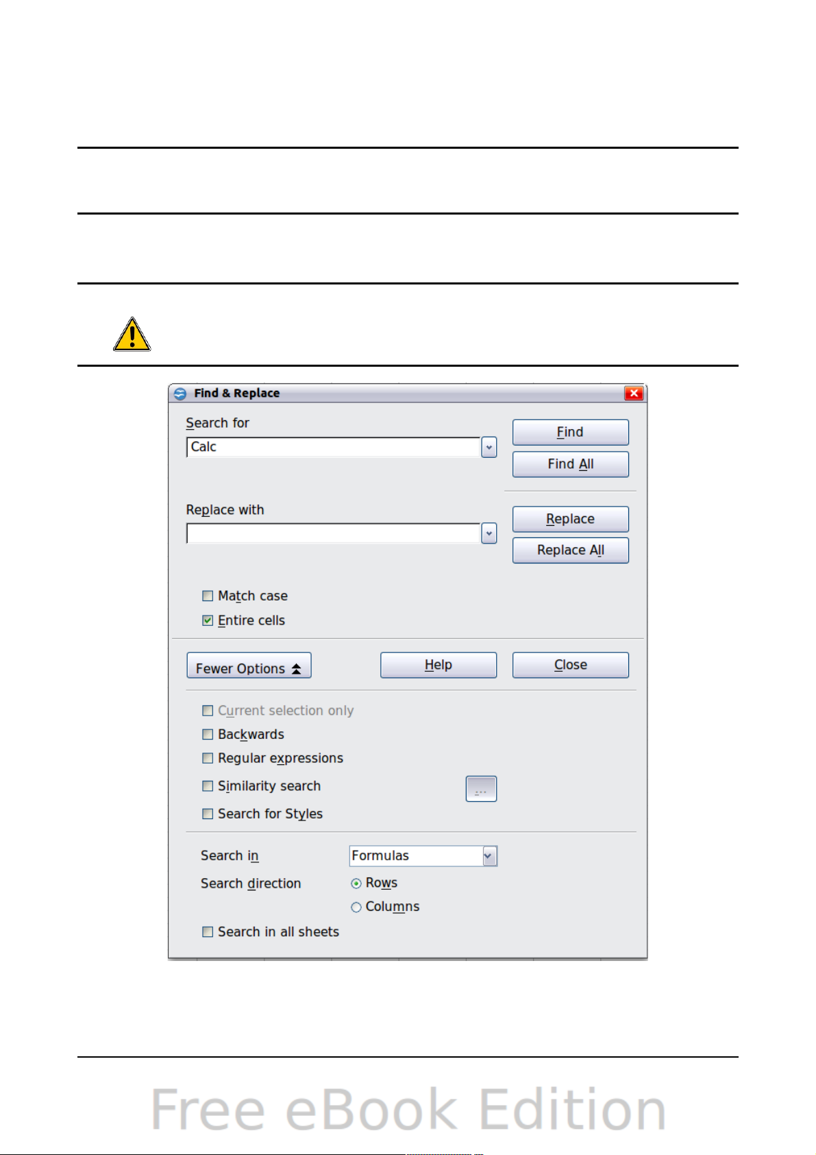
Text and numbers in cells may have been entered directly or may be the result of a calculation. The search method you use depends on the type of data you are searching for.

Tip

Cell contents can be formatted in different ways. For example, a number can be formatted as a currency, to be displayed with a currency symbol. You see the currency symbol in the cell, but you cannot search for it.

By default, Calc searches the current sheet. To search through all sheets of the document, click More Options, then select Search in all sheets option.

Caution

Use Replace All with caution; otherwise, you may end up with some highly embarrassing mistakes. A mistake with Replace All might require a manual, word-by-word search to fix, if it is not discovered in time to undo it.

66 OpenOffice.org 3.3 Calc Guide

Figure 62: Expanded Find & Replace dialog

Finding and replacing formulas or values

You can use the Find & Replace dialog to search in formulas or in the displayed values that result from a calculation.

1) To open the Find & Replace dialog, use the keyboard shortcut Control+F or select Edit > Find & Replace.

2) Click More Options to expand the dialog.

3) Select Formulas or Values in the Search in drop-down list.

• Formulas finds parts of the formulas.

• Values finds the results of the calculations.

4) Type the text you want to find in the Search for box.

5) To replace the text with different text, type the new text in the Replace with box.

6) When you have set up your search, click Find. To replace text, click Replace instead.

Finding and replacing text

1) Open the Find & Replace dialog, click More Options to expand the dialog, and select Values or Notes in the Search in drop-down list.

2) Type the text you want to find in the Search for box.

3) To replace the text with different text, type the new text in the Replace with box.

4) Click Find, Find All, Replace, or Replace All.

When you click Find, Calc selects the next cell that contains your text. You can edit the text, then click Find again to advance to the next found cell. If you closed the dialog, you can press Ctrl+Shift+F to find the next cell without opening the dialog.

When you click Find All, Calc selects all cells that contain your entry. Now you can, for example, apply a cell style to all of them at once.

Finding and replacing cell styles

To quickly change all the paragraphs of one (unwanted) style to another (preferred) style:

1) On the expanded Find & Replace dialog, select Search for Styles. The Search for and Replace with boxes now contain a list of styles.

2) Select the styles you want to search for and replace.

3) Click Find, Find All, Replace, or Replace All.

Using wildcards (regular expressions)

Wildcards (also known as regular expressions) are combinations of characters that instruct OOo how to search for something. Regular expressions are very powerful but not very intuitive. They can save time and effort by combining multiple finds into one.

To use wildcards and regular expressions when searching and replacing:

1) On the Find & Replace dialog, click More Options to see more choices. On this expanded dialog, select the Regular expressions option.

2) Type the search text, including the wildcards, in the Search for box and the replacement text (if any) in the Replace with box.

Chapter 2 Entering, Editing, and Formatting Data 67

3) Click Find, Find All, Replace, or Replace All (not recommended).

Tip

The online help describes many of the regular expressions and their uses.

The following points may be of interest to Calc users:

• In Calc, regular expressions are applied separately to each cell. This means

that a search for r.d will match red in cell A1 but will not match r in cell A2 and d (or ed) in cell A3. (The regular expression r.d means the system will try to match r followed by any other character followed by d.)

• When a match is found, the entire cell is highlighted but only the text found

will be replaced. For example, searching for brown will result in highlighting a cell containing redbrown clay, and choosing nothing in the Replace with box leaves the cell containing red clay.

• If Find is used twice in a row, and the second time the Current selection only

box is activated, then the second search will evaluate the whole of each selected cell, not just the strings that caused the cells to be selected in the first search. For example, searching for joh?n, then activating Current selection

only and searching for sm.th will find cells containing Jon Smith and Smythers, Johnathon.

• If a cell contains a hard line break (entered by Ctrl+Enter), it may be found by

using the regular expression \n. For example, if a cell contains red [hard line break] clay then searching for d\nc and entering nothing in the Replace with box leaves the cell containing relay.

• The hard line break acts to mark “end of text” (similar to “end of paragraph” in

Writer), found by the regular expression special character $, in addition to the end of text in the cell. For example, if a cell contains red [hard line break]

clay then a search for d$ replacing with al leaves the cell with real [hard line break] clay. Note that with this syntax the hard line break is not replaced.

• Using \n in the Replace with box will replace with the literal characters \n, not

a hard line break.

• The Find & Replace dialog has an option to search within formulas, values, or

notes. This option applies to any search, not just one using regular expressions. Searching with the Formulas option for SUM would find a cell containing the formula =SUM(A1:A6) as well as a cell containing the simple text SUMMARY.

• Searching for the regular expression ^$ will not find empty cells. This is

intentional, to avoid performance issues when selecting a huge number of cells. Note that empty cells will not be found even if you are only searching a selection.

• Finding cell contents using the regular expression .+ (or similar) and replacing

them with & effectively re-enters the cell contents without any formatting. This technique can be used to remove formatting automatically applied by Calc when importing data from the clipboard or from badly formatted files. For example, to convert text strings consisting of digits into actual numbers, first format the cells as numbers and then perform the search and replace.

See Chapter 7 (Using Formulas and Functions) for the use of regular expressions within formulas.

68 OpenOffice.org 3.3 Calc Guide

Chapter 3

Creating Charts and

Graphs

Presenting information visually

Introduction

Charts and graphs are often powerful ways to convey information to the reader. OpenOffice.org Calc offers a variety of chart and graph formats for your data.

Using Calc, you can customize charts and graphs to a considerable extent. Many of these options enable you to present your information in the best and clearest manner.

For readers who are interested in effective ways to present information graphically, two excellent introductions to the topic are William S. Cleveland’s The elements of

graphing data, 2nd edition, Hobart Press (1994) and Edward R. Tufte’s The Visual Display of Quantitative Information, 2nd edition, Graphics Press (2001).

Creating a chart

To demonstrate the process of making charts and graphs in Calc, we will use the small table of data in Figure 63.

To create a chart, first highlight (select) the data to be included in the chart. The selection does not need to be in a single block, as shown in Figure 64; you can also choose individual cells or groups of cells (columns or rows). See Chapter 1 (Introducing Calc) for more about selecting cells and ranges of cells.

70 OpenOffice.org 3.3 Calc Guide

Figure 63: Table of data for charting examples

Figure 64: Selecting data for plotting

Next, open the Chart Wizard dialog using one of two methods.

• Choose Insert > Chart from the menu bar.

• Or, click the Chart icon on the main toolbar.

Either method inserts a sample chart on the worksheet, opens the Formatting toolbar, and opens the Chart Wizard, as shown in Figure 66.

Tip

Before choosing the Chart Wizard, place the cursor anywhere in the area of the data. The Chart Wizard will then do a fairly good job of guessing the range of the data. Just be careful that you have not included the title of your chart.

Chapter 3 Creating Charts and Graphs 71

Figure 65: Insert chart from main toolbar

Figure 66: Chart Wizard, Step 1—Choose a chart type

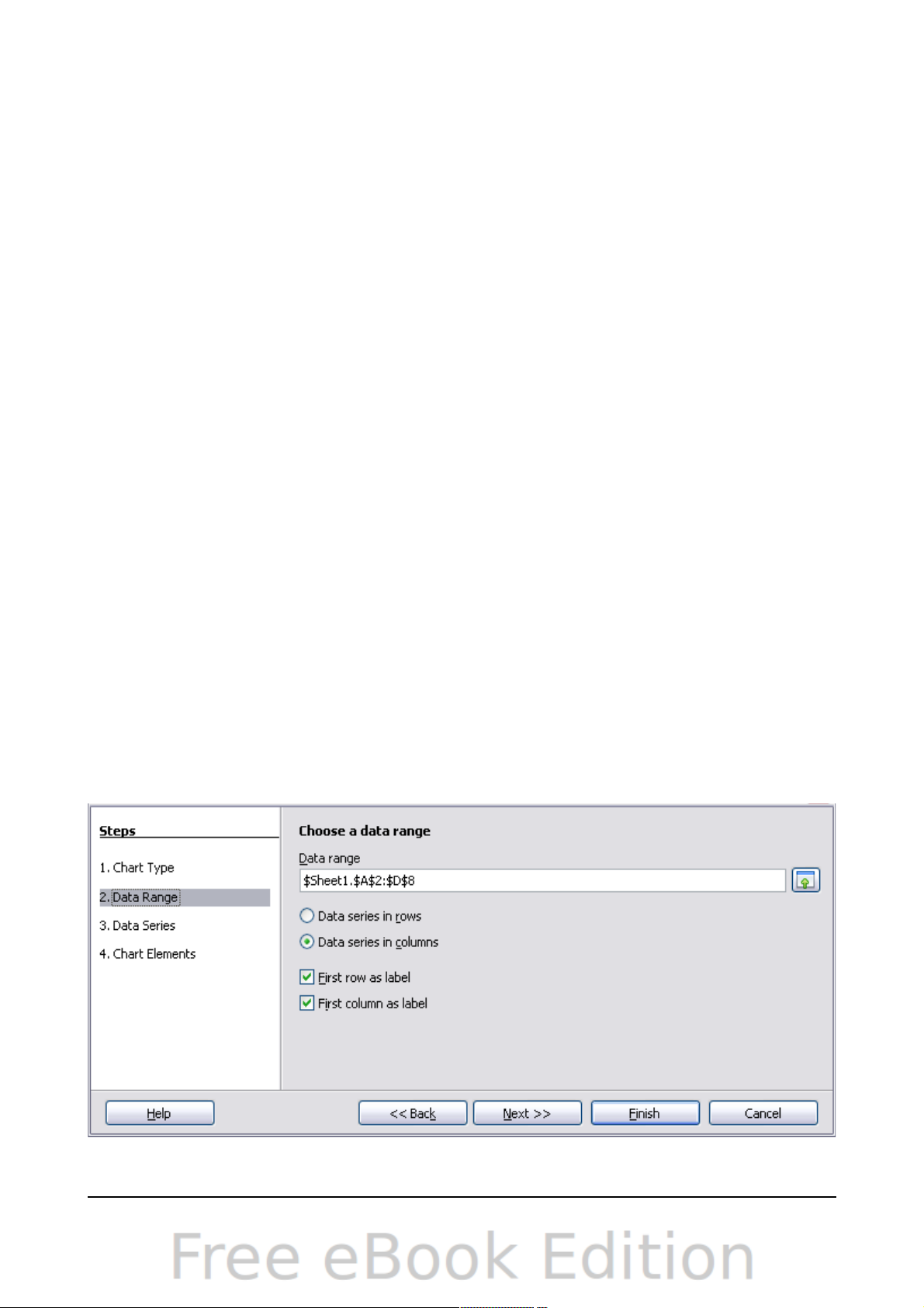
Choosing a chart type

The Chart Wizard includes a sample chart with your data. This sample chart updates to reflect the changes you make in the Chart Wizard.

The Chart Wizard has three main parts: a list of steps involved in setting up the chart, a list of chart types, and the options for each chart type. At any time you can go back to a previous step and change selections.

Calc offers a choice of 10 basic chart types, with a few options for each type of chart. The options vary according to the type of chart you pick.

The first tier of choice is for two-dimensional (2D) charts. Only those types which are suitable for 3D (Column, Bar, Pie, and Area) give you an option to select a 3D look.

On the Choose a chart type page (Figure 66), select a type by clicking on its icon. The preview updates every time you select a different type of chart, and provides a good idea of what the finished chart will look like.

The current selection is highlighted (shown with a surrounding box) on the Choose a chart type page. The chart’s name is shown just below the icons. For the moment, we will stick to the Column chart and click on Next again.

Changing data ranges and axes labels

In Step 2, Data Range, you can manually correct any mistakes you have made in selecting the data.

On this page you can also change the way you are plotting the data by using the rows —rather than the columns—as data series. This is useful if you use a style of chart such as Donut or Pie to display your data.

Lastly, you can choose whether to use the first row or first column, or both, as labels on the axes of the chart.

You can confirm what you have done so far by clicking the Finish button, or click Next to change some more details of the chart.

We will click Next to see what we can do to our chart using the other pages of the Wizard.

72 OpenOffice.org 3.3 Calc Guide

Figure 67: Changing data ranges and axes labels

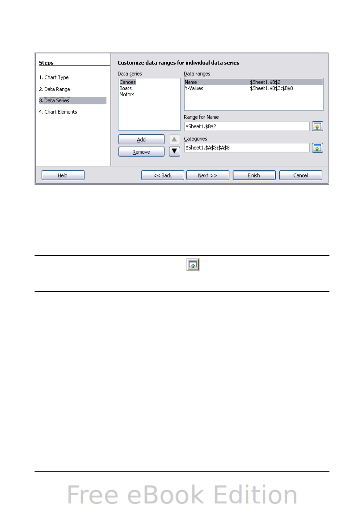
Selecting data series

On the Data Series page, you can fine tune the data that you want to include in the chart. Perhaps you have decided that you do not want to include the data for canoes. If so, highlight Canoes in the Data series box and click on Remove. Each named data series has its ranges and its individual Y-values listed. This is useful if you have very specific requirements for data in your chart, as you can include or leave out these ranges.

Tip

You can click the Shrink button next to the Range for Name box to work on the spreadsheet itself. This is handy if your data ranges are larger than ours and the Chart Wizard is in the way.

Another way to plot any unconnected columns of data is to select the first data series and then select the next series while holding down the Ctrl key. Or you can type the columns in the text boxes. The columns must be separated by semi-colons. Thus, to plot B3:B11 against G3:G11, type the selection range as B3:B11;G3:G11.

The two data series you are selecting must be in separate columns or rows. Otherwise Calc will assume that you are adding to the same data series.

Click Next to deal with titles, legend and grids.

Adding or changing titles, legend, and grids

On the Chart Elements page (Figure 69), you can give your chart a title and, if desired, a subtitle. Use a title that draws the viewers’ attention to the purpose of the chart: what you want them to see. For example, a better title for this chart might be The Performance of Motor and Other Rental Boats.

It may be of benefit to have labels for the x-axis or the y-axis. This is where you give viewers an idea as to the proportion of your data. For example, if we put Thousands in the y-axis label of our graph, it changes the scope of the chart entirely. For ease of estimating data you can also display the x- or y- axis grids by selecting the Display

grids options.

Chapter 3 Creating Charts and Graphs 73

Figure 68: Amending data series and ranges

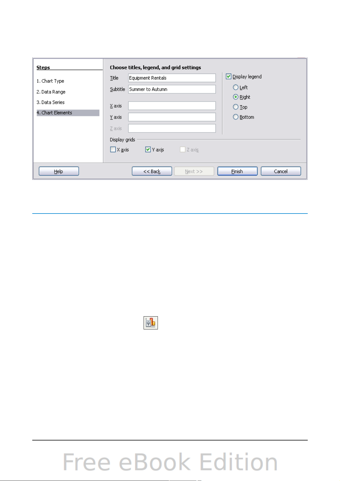
You can leave out the legend or include it and place it to the left, right, top or bottom.

To confirm your selections and complete the chart, click Finish.

Editing charts

After you have created a chart, you may find things you would like to change. Calc provides tools for changing the chart type, chart elements, data ranges, fonts, colors and many other options, through the Insert and Format menus, the right-click (context) menu and the Chart toolbar.

Changing the chart type

You can change the chart type at any time. To do so:

1) First select the chart by double-clicking on it. The chart should now be surrounded by a gray border.

2) Then do one of the following:

• Choose Format > Chart Type from the menu bar.

• Click the chart type icon on the Formatting toolbar.

• Right-click on the chart and choose Chart Type.

In each case, a dialog similar to the one in Figure 66 opens. See page 72 for more information.

Adding or removing chart elements

Figures 70 and 71 show the elements of 2D and 3D charts.

The default 2D chart includes only two of those elements:

• Chart wall contains the graphic of the chart displaying the data.

• Chart area is the area surrounding the chart graphic. The (optional) chart title

and the legend (key) are in the chart area.

74 OpenOffice.org 3.3 Calc Guide

Figure 69: Titles, legend and grids

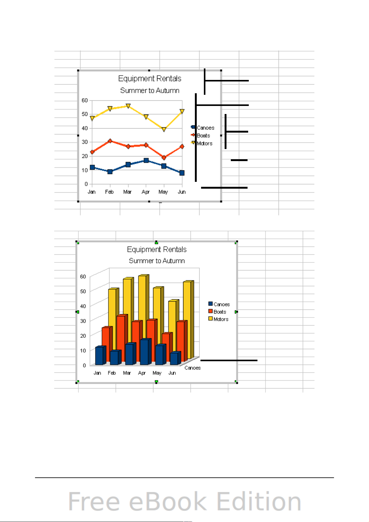
The default 3D chart also has the chart floor, which is not available in 2D charts.

You can add other elements using the commands on the Insert menu. The various choices open dialogs in which you can specify details.

First select the chart so the green sizing handles are visible. This is done with a single click on the chart.

The dialogs for Titles, Legend, Axes and Grids are self-explanatory. The others are a bit more complicated, so we’ll take a look at them here.

Chapter 3 Creating Charts and Graphs 75

Chart area

Chart wall

Chart title

Legend

Axis labels

Chart floor

Figure 70: Elements of 2D chart

Figure 71: Elements of 3D chart

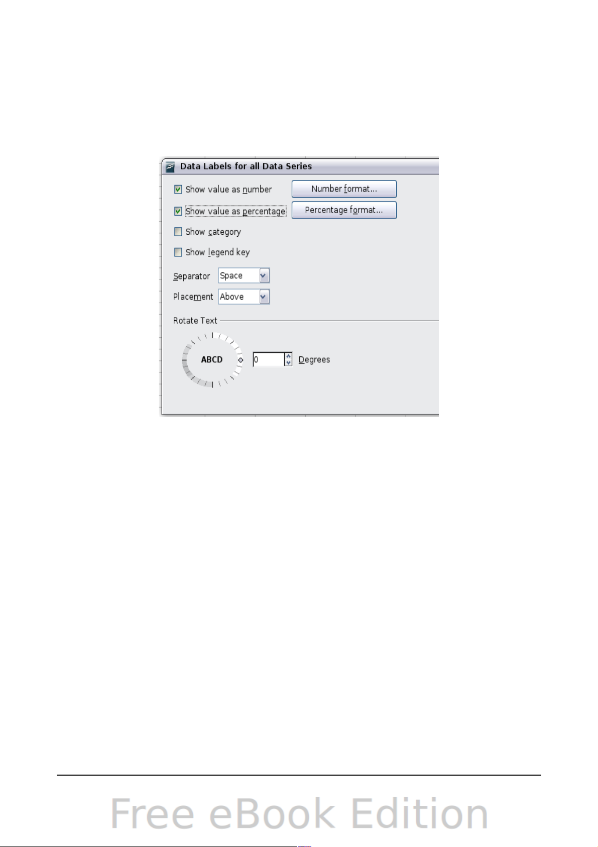
Data labels

Data labels put information about each data point on the chart. They can be very useful for presenting detailed information, but you need to be careful to not create a chart that is too cluttered to read.

Select the graph as described above and choose Insert > Data Labels. The options are as follows.

Show value as number

Displays the numeric values of the data points. When selected, this option activates the Number format... button.

Number format...

Opens the Number Format dialog, where you can select the number format. This dialog is very similar to the one for formatting numbers in cells, described in Chapter 2 (Entering, Editing, and Formatting Data).

Show value as percentage

Displays the percentage value of the data points in each column. When selected, this option activates the Percentage format... button.

Percentage format...

Opens the Number Format dialog, where you can select the percentage format.

Show category

Shows the data point text labels.

Show legend key

Displays the legend icons next to each data point label.

Separator

Selects the separator between multiple text strings for the same object.

76 OpenOffice.org 3.3 Calc Guide

Figure 72: Data Labels dialog

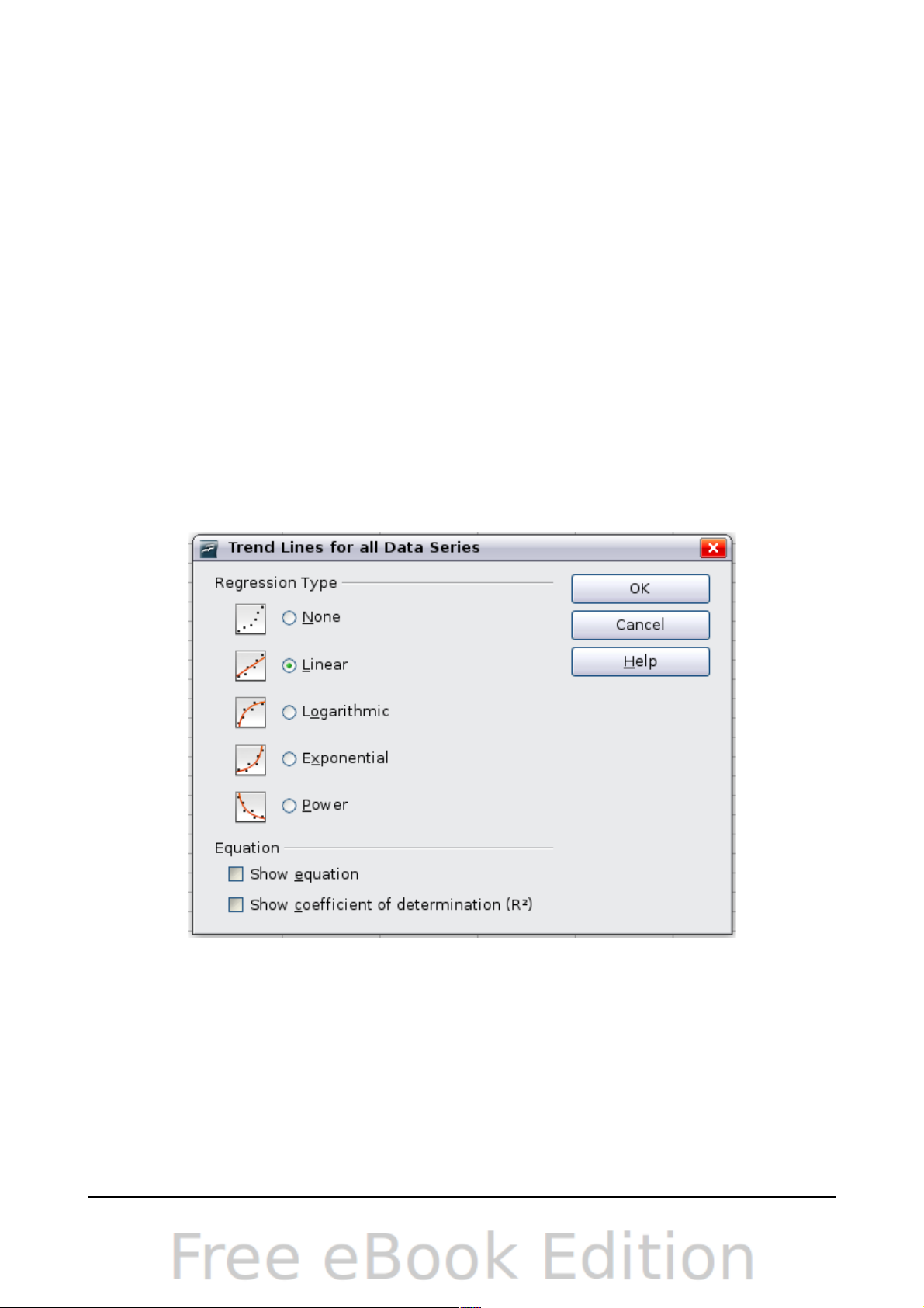
Placement

Selects the placement of data labels relative to the objects.

Figure 77 on page 83 shows examples of values as text (neither Show value as number nor Show value as percentage selected) and values as percentages, as well as when data values are used as substitutes for legends or in conjunction with them.

Trend lines

When you have a scattered grouping of points in a graph, you may want to show the relationship of the points. A trend line is what you need. Calc has a good selection of regression types you can use for trend lines: linear, logarithm, exponential, and power. Choose the type that comes closest to passing through all of the points.

To insert trend lines for all data series, double-click the chart to enter edit mode. Choose Insert > Trend Lines, then select the type of trend line from None, Linear, Logarithmic, Exponential, or Power. You can also choose whether to show the equation for the trend line and the coefficient of determination (R2).

To insert a trend line for a single data series, first select the data series in the chart, and then right-click and choose Insert > Trend Line from the context menu. The dialog for a single trend line is similar to the one below but has a second tab (Line), where you can choose attributes (style, color, width, and transparency) of the line.

To delete a single trend line or mean value line, click the line, then press the Del key.

To delete all trend lines, choose Insert > Trend Lines, then select None.

A trend line is shown in the legend automatically.

If you insert a trend line on a chart type that uses categories, such as Line or Column, then the numbers 1, 2, 3, … are used as x-values to calculate the trend line.

Chapter 3 Creating Charts and Graphs 77

Figure 73: Trend Lines dialog

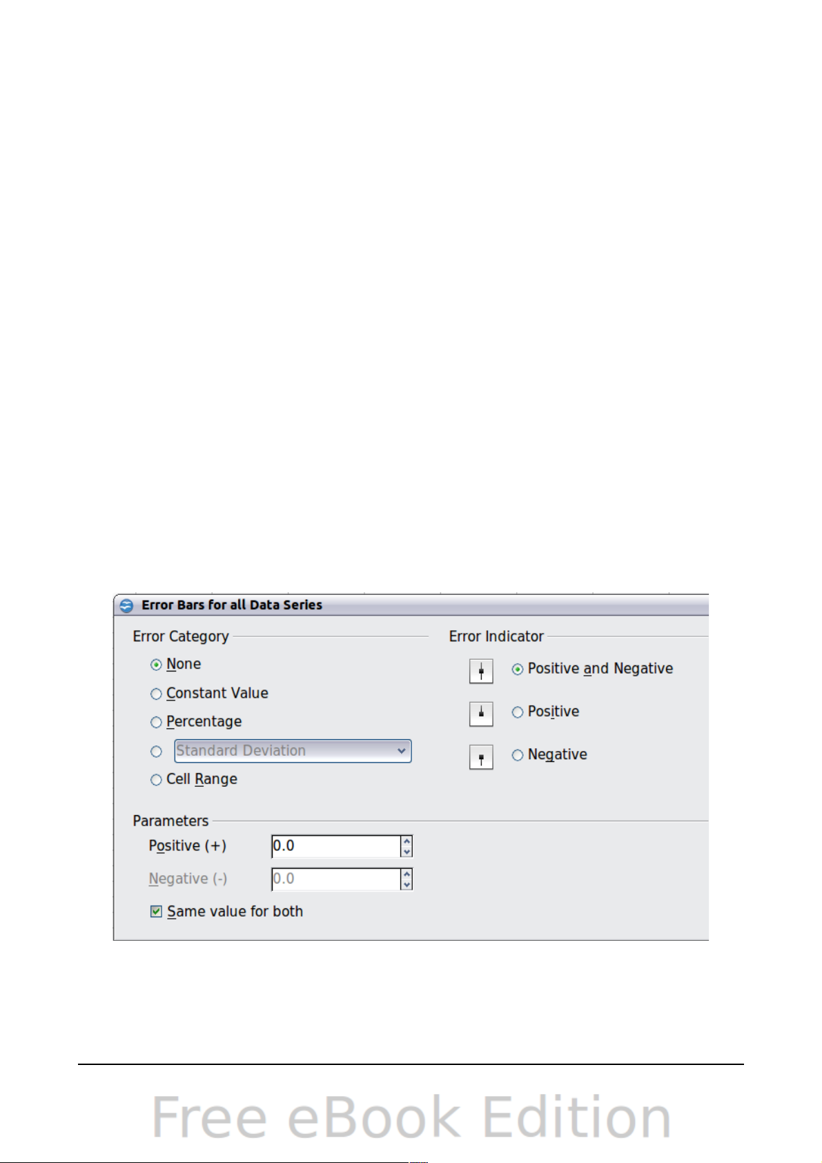
The trend line has the same color as the corresponding data series. To change the line properties, select the trend line and choose Format Trend Line. This opens the Line tab of the Trend Lines dialog.

To show the trend line equation, select the trend line in the chart, right-click to open the context menu, and choose Insert Trend Line Equation.

When the chart is in edit mode, OpenOffice.org gives you the equation of the trend line and the correlation coefficient. Click on the trend line to see the information in the status bar. To show the equation and the correlation coefficient, select the line and choose Insert R2 and Trend Line Equation.

For more details on the regression equations, see the topic Trend lines in charts in the Help.

Mean value lines

If you select the Mean Value Lines dialog from the Insert menu, Calc calculates the average of each selected data series and places a colored line at the correct level in the chart.

Y error bars

If you are presenting data that has a known possibility of error, such as social surveys using a particular sampling method, or you want to show the measuring accuracy of the tool you used, you may wish to show error bars on the chart. Select the chart and choose Insert > Y Error Bars.

Several options are provided on the Error Bars dialog. You can only choose one option at a time. You can also choose whether the error indicator shows both positive and negative errors, or only positive or only negative.

• Constant Value – you can have separate positive and negative values.

• Percentage – choose the error as a percentage of the data points.

78 OpenOffice.org 3.3 Calc Guide

Figure 74: Specifying the parameters of error bars

• In the drop-down list: – Standard Error – calculates the error based on the numerical data you

provide in the chart

– Variance – shows error calculated on the size of the biggest and smallest

data points

– Standard Deviation – shows error calculated on standard deviation – Error Margin – you designate the error

• Cell Range – calculates the error based on cell ranges you select. The

Parameters section at the bottom of the dialog changes to allow selection of the cell ranges.

Formatting charts

The Format menu has many options for formatting and fine-tuning the appearance of your charts.

Double-click the chart so that it is enclosed by a gray border indicating edit mode; then, select the chart element that you want to format. Choose Format from the menu bar, or right-click to display a context menu relevant to the selected element. The formatting choices are as follows.

Format Selection

Opens a dialog in which you can specify the area fill, borders, transparency, characters, font effects, and other attributes of the selected element of the chart (see page 85).

Position and Size

Opens a dialog (see page 88).

Arrangement

Provides two choices: Bring Forward and Send Backward, of which only one may be active for some items. Use these choices to arrange overlapping data series.

Title

Formats the titles of the chart and its axes.

Legend

Formats the location, borders, background, and type of the legend.

Axis

Formats the lines that create the chart as well as the font of the text that appears on both the X and Y axes.

Grid

Formats the lines that create a grid for the chart.

Chart Wall, Chart Floor, Chart Area

These functions are described in the following sections.

Chart Type

Changes what kind of chart is displayed and whether it is two- or threedimensional.

Chapter 3 Creating Charts and Graphs 79

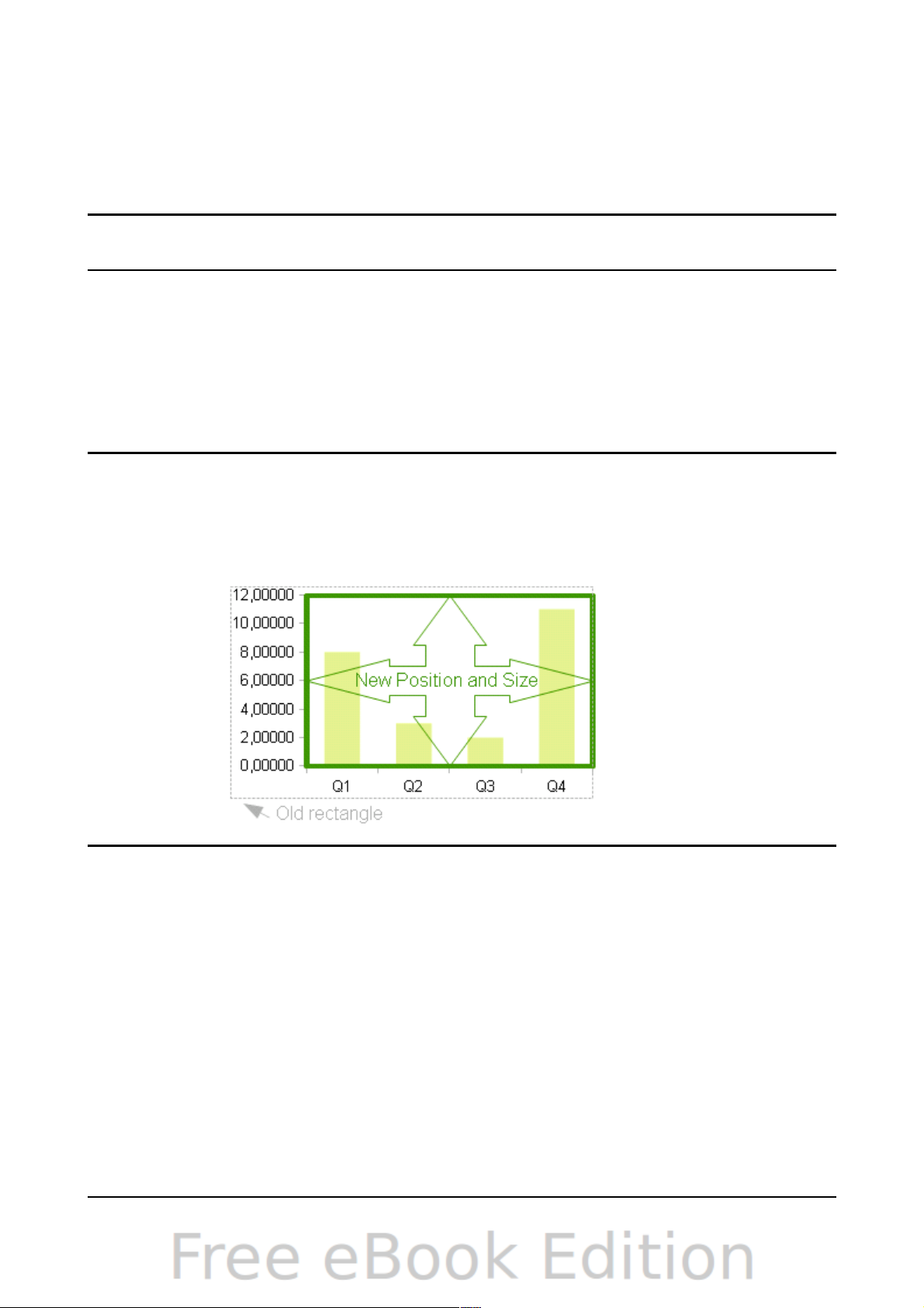
Data Ranges

Explained on page 72 (Figure 67 and Figure 68).

3D View

Formats 3D charts (see page 82).

Note

Chart Floor and 3D View are only available for a 3D chart. These options are unavailable (grayed out) if a 2D chart is selected.

In most cases you need to select the exact element you want to format. Sometimes this can be tricky to do with the mouse, if the chart has many elements, especially if some of them are small or overlapping. If you have Tooltips turned on (in Tools > Options > OpenOffice.org > General > Help, select Tips), then as you move the mouse over each element, its name appears in the Tooltip. Once you have selected one element, you can press Tab to move through the other elements until you find the one you want. The name of the selected element appears in the Status Bar.

Note

Until OOo 3.2.1, axis labels and axis titles were included in the positioning rectangle of the chart. The space required for those labels depends on many factors like scaling, font, font size, and so on. To prevent the data plot itself from changing size and position, the labels are no longer included in the diagram size, so you can set the position and size of the plot area directly.

Moving chart elements

You may wish to move or resize individual elements of a chart, independent of other chart elements. For example, you may wish to move the legend to a different place. Pie charts allow moving of individual wedges of the pie (in addition to the choice of “exploding” the entire pie).

1) Double-click the chart so that it is enclosed by a gray border.

2) Double-click any of the elements—the title, the legend, or the chart graphic. Click and drag to move the element. If the element is already selected, then move the pointer over the element to get the move icon (small hand), then click, drag and move the element.

3) Release the mouse button when the element is in the desired position.

80 OpenOffice.org 3.3 Calc Guide

Note

If your chart graphic is 3D, round red handles appear which control the three-dimensional angle of the graphic. You cannot resize or reposition the graphic while the round red handles are showing. With the round red handles showing, Shift+Click to get the green resizing handles. You can now resize and reposition your 3D chart graphic. See the following tip.

Tip

You can resize the chart graphic using its green resizing handles (Shift+Click, then drag a corner handle to maintain the proportions). However, you cannot resize the title or the key.

Changing the chart area background

The chart area is the area surrounding the chart graphic, including the (optional) main title and key.

1) Double-click the chart so that it is enclosed by a gray border.

2) Choose Format > Chart Area or right-click on the chart area and choose Format Chart Area.

3) On the Chart Area dialog, choose the desired format settings.

On the Area tab, you can change the color, or choose a hatch pattern, bitmap or some preset gradients. Click on the drop-down box to see the options. Patterns are probably more useful than color if you have to print out your chart in black and white.

You can also use the Transparency tab to change the area’s transparency. If you used a preset gradient from the Area tab, you can see the different parameters of which it is composed.

Chapter 3 Creating Charts and Graphs 81

Figure 75: Chart Area dialog

Changing the chart graphic background

The chart wall is the area that contains the chart graphic.

1) Double-click the chart so that it is enclosed by a gray border.

2) Choose Format > Chart Wall. The Chart Wall dialog has the same formatting options as described in “Changing the chart area background” above.

3) Choose your settings and click OK.

Changing colors

If you need a different color scheme from the default for the charts in all your documents, go to Tools > Options > Charts > Default Colors, which has a much wider range of colors to choose from. Changes made in this dialog affect the default chart colors for any chart you make in future.

Formatting 3D charts

Use Format > 3D View to fine tune 3D charts. The 3D View dialog has three pages, where you can change the perspective of the chart, determine whether the chart uses the simple or realistic schemes or your own custom scheme, and the illumination that controls where the shadows will fall.

Rotation and perspective

To rotate a 3D chart or view it in perspective, enter the required values on the Perspective tab of the 3D View dialog. You can also rotate 3D charts interactively; see page 84.

Here are some hints for using the Perspective tab:

• Set all angles to 0 for a front view of the chart. Pie charts and donut charts are

shown as circles.

• With Right-angled axes enabled, you can rotate the chart contents only in the X

and Y direction; that is, parallel to the chart borders.

82 OpenOffice.org 3.3 Calc Guide

Figure 76: Rotating a chart

• An x value of 90, with y and z set to 0, provides a view from the top of the

chart. With x set to –90, the view is from the bottom of the chart.

• The rotations are applied in the following order: x first, then y, and z last.

• When shading is enabled and you rotate a chart, the lights are rotated as if

they are fixed to the chart.

• The rotation axes always relate to the page, not to the chart’s axes. This is

different from some other chart programs.

• Select the Perspective option to view the chart in central perspective as

through a camera lens instead of using a parallel projection.

• Set the focus length in the box next to the Perspective option (it becomes

active when you select the option). 100% gives a perspective view where a far edge in the chart looks approximately half as big as a near edge.

Appearance

Use the Appearance page to modify some aspects of a 3D chart’s appearance.

Select a scheme from the list box. When you select a scheme, the options and the light sources are set accordingly. If you select or deselect a combination of options that is not given by the Realistic or Simple schemes, you can create a Custom scheme.

Select Shading to use the Gouraud method for rendering the surface, which applies gradients for a smoother, more realistic look. Otherwise, a flat method is used. The flat method sets a single color and brightness for each polygon. The edges are visible, soft gradients and spot lights are not possible. Refer to the Draw Guide for more details on shading.

Select Object Borders to draw lines along the edges.

Select Rounded Edges to smooth the edges of box shapes. In some cases this option is not available.

Chapter 3 Creating Charts and Graphs 83

Figure 77: Modifying appearance of 3D chart

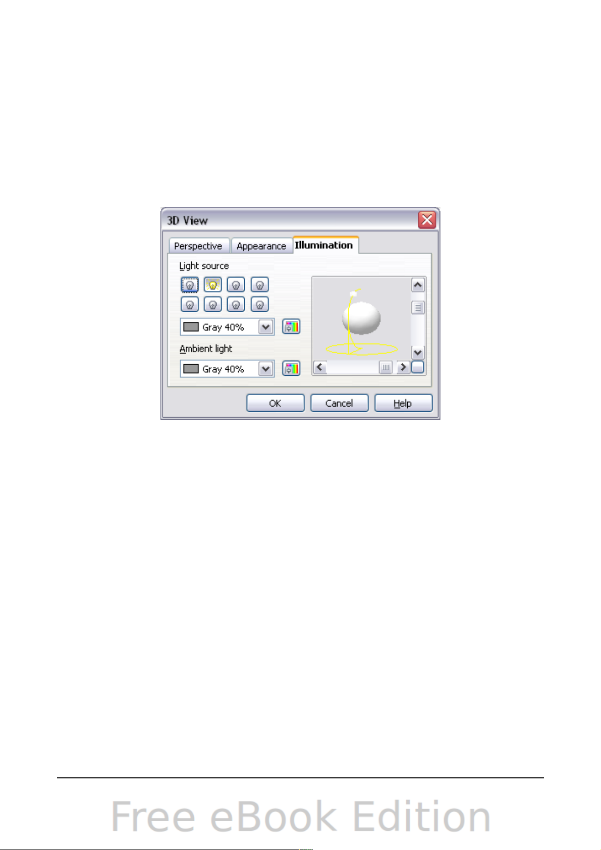
Illumination

Use the Illumination page (Figure 78) to set the light sources for the 3D view. Refer to the Draw Guide for more details on setting the illumination.

Click any of the eight buttons to switch a directed light source on or off. By default, the second light source is switched on. It is the first of seven normal, uniform light sources. The first light source projects a specular light with highlights.

For the selected light source, you can then choose a color and intensity in the list just below the eight buttons. The brightness values of all lights are added, so use dark colors when you enable multiple lights.

Each light source always points at the middle of the object initially. To change the position of the light source, use the small preview inside this page. It has two sliders to set the vertical and horizontal position of the selected light source.

The button in the corner of the small preview switches the internal illumination model between a sphere and a cube.

Use the Ambient light list to define the ambient light which shines with a uniform intensity from all directions.

Rotating 3D charts interactively

In addition to using the Perspective page of the 3D View dialog to rotate 3D charts, you can also rotate them interactively.

Select the Chart Wall, then hover the mouse pointer over a corner handle or the rotation symbol found in the middle of the chart’s information grid. The cursor changes to a rotation icon.

Press and hold the left mouse button and drag the corner in the direction you wish. A dashed outline of the chart is visible while you drag, to help you see how the result will look.

84 OpenOffice.org 3.3 Calc Guide

Figure 78: Setting the illumination

Formatting the chart elements

Depending on the purpose of your document, for example a screen presentation or a printed document for a black and white publication, you might wish to use more detailed control over the different chart elements to give you what you need.

To format an element, left-click on the element that you wish to change, for example one of the axes. The element will be highlighted with green squares. Then, right-click and choose an item from the context menu. Each chart element has its own selection of items. In the next few sections, we explore some of those options.

Formatting axes and inserting grids

Sometimes you need to have a special scale for one of the axes of your chart, or you need smaller grid intervals, or you want to change the formating of the labels on the axis. After highlighting the axis you wish to change, right-click and choose one of the items from the pop-up menu.

Choosing Format > Axis > X Axis or Format > Axis > Y Axis opens the dialog shown in Figure 79, which in this case is the Scale tab. The fields available on this dialog depend on the type of chart and whether it is 2D or 3D.

On the Scale tab, you can choose a logarithmic or linear scale (default), how many marks you need on the line, where the marks are to appear and the increments (intervals) of the scale. You must first deselect the Automatic option in order to modify the value for any scale. Selecting the Reverse direction radial creates a backwards representation of the chart.

On the Label tab (Figure 80), you can choose whether to show or hide the labels and how to handle them when they won’t all fit neatly into one row (for example, if the words are too long).

Not shown here are the tabs with options for choosing a font and specific font effects, formatting the lines, positioning the elements of the line and interval marks, and selecting effects relating to Asian Typography if this function has been activated in Tools > Options > Languages.

Chapter 3 Creating Charts and Graphs 85

Figure 79: Formatting axis scales

Figure 80: Formatting axis labels

Formating data labels

You can choose properties for the labels of the data series. Carefully click on the chart element, then right-click and choose the property you want to change. Choosing the command Format Data Labels opens a dialog with several tabs where you can change the color of the label text, the size of the font, and other attributes. The Data Label tab is shown in Figure 72.

On the Data Label tab, you can choose whether to:

• Show the labels as text

• Show numeric values as a percentage or a number

• Include the legend box as part of the label

The text for labels is taken from the column labels and it cannot be changed here. If the text needs to be abbreviated, or if it did not label your graph as you were expecting, you need to change it in the original data table.

Hierarchical axis labels

Multiple columns of categories are now displayed in a hierarchical manner at the axis as shown. To get that automatically while creating a chart, make sure that all the first columns (or rows) contain text and not only numbers. You can also choose to set the ranges for categories to multiple columns on the Data Series page in the Wizard or the Data Ranges dialog.

86 OpenOffice.org 3.3 Calc Guide

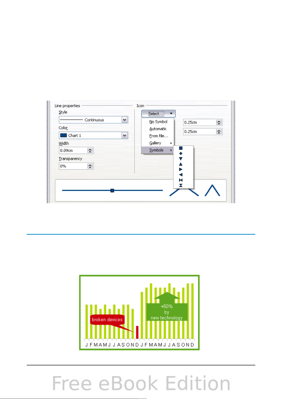
Choosing and formatting symbols

In line and scatter charts the symbols representing the points can be changed to a different symbol shape or color through the object properties dialog. Select the data series you wish to change, right-click, and choose Format Data Series from the context menu. You can reach this dialog by double-clicking the area of data you would like to change.

On the Line tab of the Data Series dialog, in the Icon section, choose from the dropdown list Select > Symbols. Here you can choose no symbol, a symbol from an inbuilt selection, a more exciting range from the gallery, or if you have pictures you need to use instead, you can insert them using Select > From file.

Adding drawing objects to charts

(New in OOo 3.3) As in the other OOo components, you can use the drawing toolbar to add simple shapes such as lines, rectangles, and text objects, or more complex shapes such as symbols or block arrows. This toolbar is located at the bottom of the screen and automatically appears when a chart is generated. Use these additional shapes to add explanatory notes to your chart as demonstrated in the figure below.

Chapter 3 Creating Charts and Graphs 87

Figure 81: Symbol selection

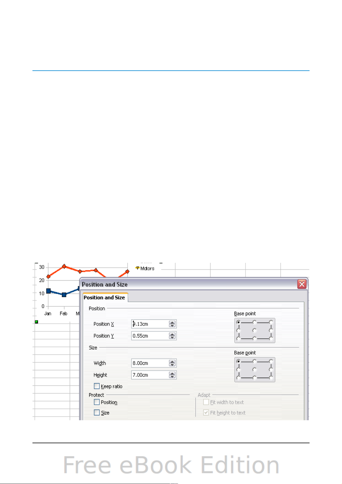
To format the drawing objects, right-click and choose your changes from the context menu.

Resizing and moving the chart

You can resize or move all elements of a chart at the same time, in two ways: interactively or by using the Position and Size dialog. You may wish to use a combination of both methods: interactive for quick and easy changes, then the dialog for precise sizing and positioning.

To resize a chart interactively:

1) Click once on the chart to select it. Green sizing handles appear around the chart.

2) To increase or decrease the size of the chart, click and drag one of the markers in one of the four corners of the chart. To maintain the correct ratio of the sides, hold the Shift key down while you click and drag.

To move a chart interactively:

1) Click on the chart to select it. Green sizing handles appear around the chart.

2) Hover the mouse pointer anywhere over the chart. When it changes to the move icon, click and drag the chart to its new location.

3) Release the mouse button when the element is in the desired position.

Using the Position and Size dialog

To resize or move a chart using the Position and Size dialog:

1) Click on the chart to select it. Green sizing handles appear around the chart.

2) Right-click and choose Position and Size from the pop-up menu.

3) Make your choices on this dialog.

88 OpenOffice.org 3.3 Calc Guide

Figure 82: Defining the position and size of an object

Position is defined as a X,Y coordinate relative to a fixed point (the base point), typically located at the upper left of the document. You can temporarily change this base point to make positioning or dimensioning simpler (click on the spot corresponding to the location of the base point in either of the two selection windows on the right side of the dialog—upper for positioning or lower for dimensioning).

The possible base point positions correspond to the handles on the selection frame plus a central point. The change in position lasts only as long as you have the dialog open; when you close this dialog, Calc resets the base point to the standard position.

Tip

The Keep ratio option is very useful. Select it to keep the ratio of width to height fixed while you change the size of an object.

Either or both the size and position can be protected so that they cannot be accidentally changed. Select the appropriate options.

Tip

If you cannot move an object, check to see if its position is protected.

Gallery of chart types

Its important to remember that while your data can be presented with a number of different charts, the message you want to convey to your audience dictates the chart you ultimately use. The following sections present examples of the types of charts that Calc provides, with some of the tweaks that each sort can have and some notes as to what purpose you might have for that chart type. For further details, see the OpenOffice.org Help index.

Column charts

Column charts are commonly used for data that shows trends over time. They are best for charts that have a relatively small number of data points. (For a larger time series, a line chart would be better.) It is the default chart type, as it is one of the most useful charts and the easiest to understand.

Bar charts

Chapter 3 Creating Charts and Graphs 89

Figure 83: Three bar graph treatments.

Bar charts are excellent for giving an immediate visual impact for data comparison in

cases when time is not an important factor, for example when comparing the popularity of a few products in a marketplace.

• The first chart in Figure 83 is achieved quite simply by using the chart wizard

with Insert > Grids, deselecting y-axis, and using Insert > Mean Value

Lines.

• The second chart in the figure is the 3D option in the chart wizard with a

simple border and the 3D chart area twisted around.

• The third chart in the figure is an attempt to get rid of the legend and put

labels showing the names of the companies on the axis instead. We also changed the colors to a hatch pattern.

Pie charts

Pie charts are excellent when you need to compare proportions. For example, a pie chart would be ideal if you needed to figure out comparisons of departmental spending, what the department spent on different items or what different departments spent. These charts work best with smaller numbers of values, no more than about half a dozen. Any more than this and the visual impact starts to fade.

As the Chart Wizard guesses the series that you wish to include in your pie chart, you might need to adjust this initially on the Wizard’s Data Ranges page if you know you want a pie chart or by using the Format > Data Ranges > Data Series dialog.

You can do some interesting things with a pie chart, especially if you make it into a 3D chart. It can then be tilted, given shadows, and generally turned into a work of art.

You can choose an option in the Chart Wizard to explode the pie chart, but this is an all-or-nothing option. If your aim is to accentuate one piece of the pie, you can separate out one piece by carefully highlighting it after you have finished with the Chart Wizard, and dragging it out of the group. When you do this, you might need to enlarge the chart area again to regain the original size of the pieces.

The effects achieved in Figure 84 are explained below.

• The first example is a 2D pie chart with one part of the pie exploded. To produce

this type of chart, first choose Insert > Legend and deselect Display legend. Choose Insert > Data Labels and choose Show value as number. Then carefully select the piece you wish to highlight, move the cursor to the edge of the piece and click (the piece will have nine green highlight squares to mark it), and then drag it

90 OpenOffice.org 3.3 Calc Guide

Figure 84: Pie charts

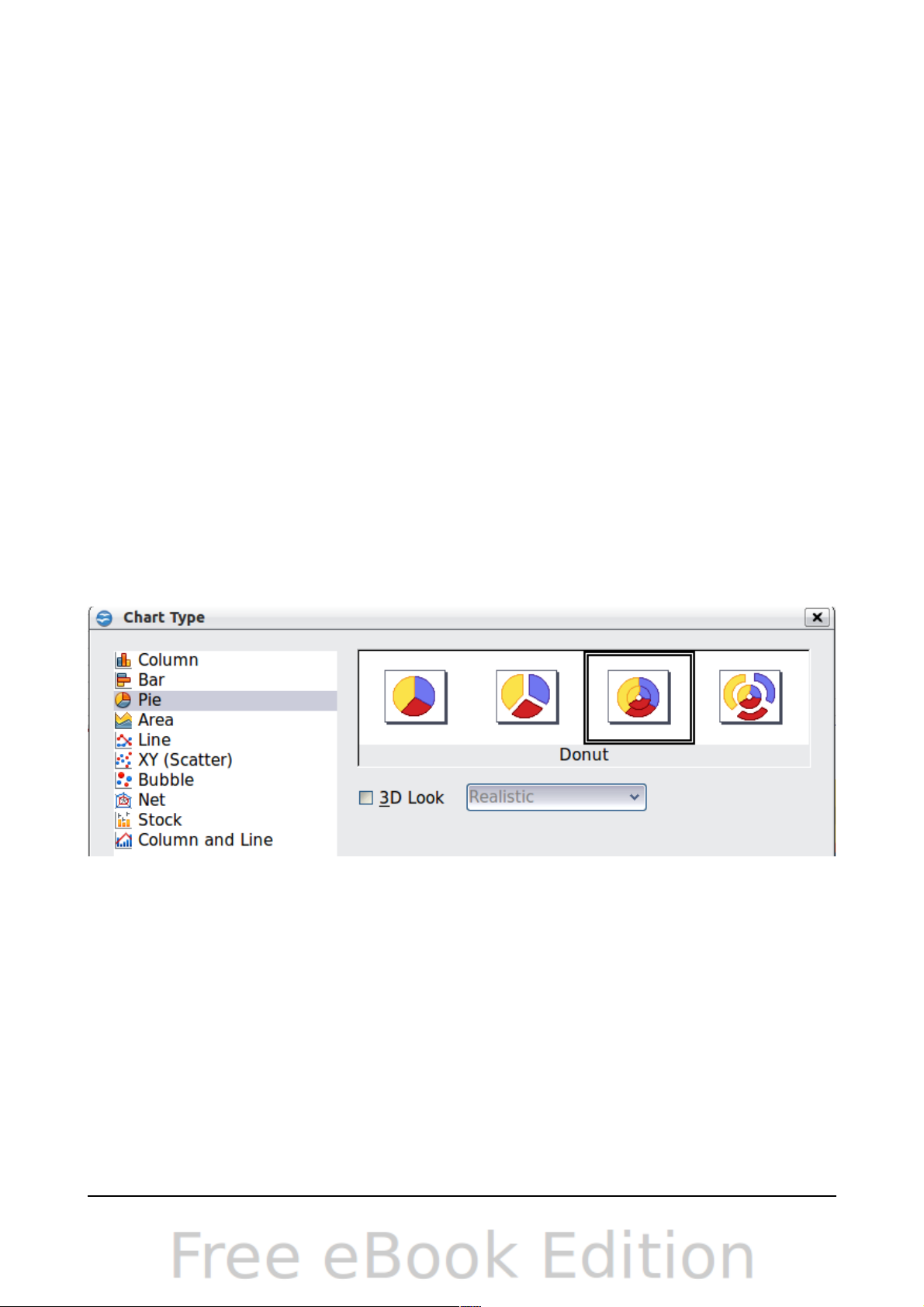
out from the rest of the pieces. The pieces will decrease in size, so you need to highlight the chart wall and drag it at a corner to increase the size.

• The second example is a 3D pie chart with realistic schema and illumination. With

a completed 2D pie chart, choose Format > 3D view > Illumination where you can change the direction of the light, the color of the ambient light, and the depth of the shade. We also adjusted the 3D angle of the disc in the Perspective dialog on the same set of tabs.

The chart updates as you make changes, so you can immediately see the effects.

If you want to separate out one of the pieces, click on it carefully; you should see a wire frame highlight. Drag it out with the mouse and then, if necessary, increase the size of the chart wall.

• The third example is a 3D pie chart with different fill effects in each portion of the

pie. Choose Insert > Data labels and select Show value as percentage. Carefully select each of the pieces so that it has a wire frame, then highlight and right-click to get the object properties dialog. Choose the Area tab. For one of the pieces we chose a bitmap effect, for another we selected a gradient feature and for the third we used the Transparency tab and adjusted the transparency to 50%.

Donut charts

Donut charts are a variation on the pie chart. To create one, choose Pie in the Chart Type dialog, and choose the third or fourth type of pie chart. For more variety, consider selecting 3D Look.

Chapter 3 Creating Charts and Graphs 91

Figure 85: Choosing a donut chart

Figure 86: Examples of donut charts

Area charts

An area chart is a version of a line or column graph. It may be useful where you wish to emphasize volume of change. Area charts have a greater visual impact than a line chart, but the data you use will make a difference.

As shown in Figure 87, an area chart is sometimes tricky to use. This may be one good reason to use transparency values in an area chart. After setting up the basic chart using the Chart Wizard, do the following:

• Right-click on the y-axis and choose Delete Major Grid. As the data overlaps,

some of it is is lost behind the first data series. This is not what you want. A better solution is shown in the highlighted chart below and is explained in the next point.

• After deselecting the y-axis grid, right-click on each data series in turn and

choose Format Data Series. On the Transparency tab, set Transparency to 50%. The transparency makes it easy to see the data hidden behind the first data series. Now, right-click on the x-axis and choose Format Axis. On the Label tab, choose Tile in the Order section and set the Text orientation to 55 degrees. This places the long labels at an angle.

• To create the third variation, after doing the steps above, right-click and

choose Chart Type. Choose the 3D Look option and select Realistic from the drop-down list. We also twisted the chart area around and gave the chart wall

92 OpenOffice.org 3.3 Calc Guide

Figure 87: Area charts—the good, the bad, and the ugly

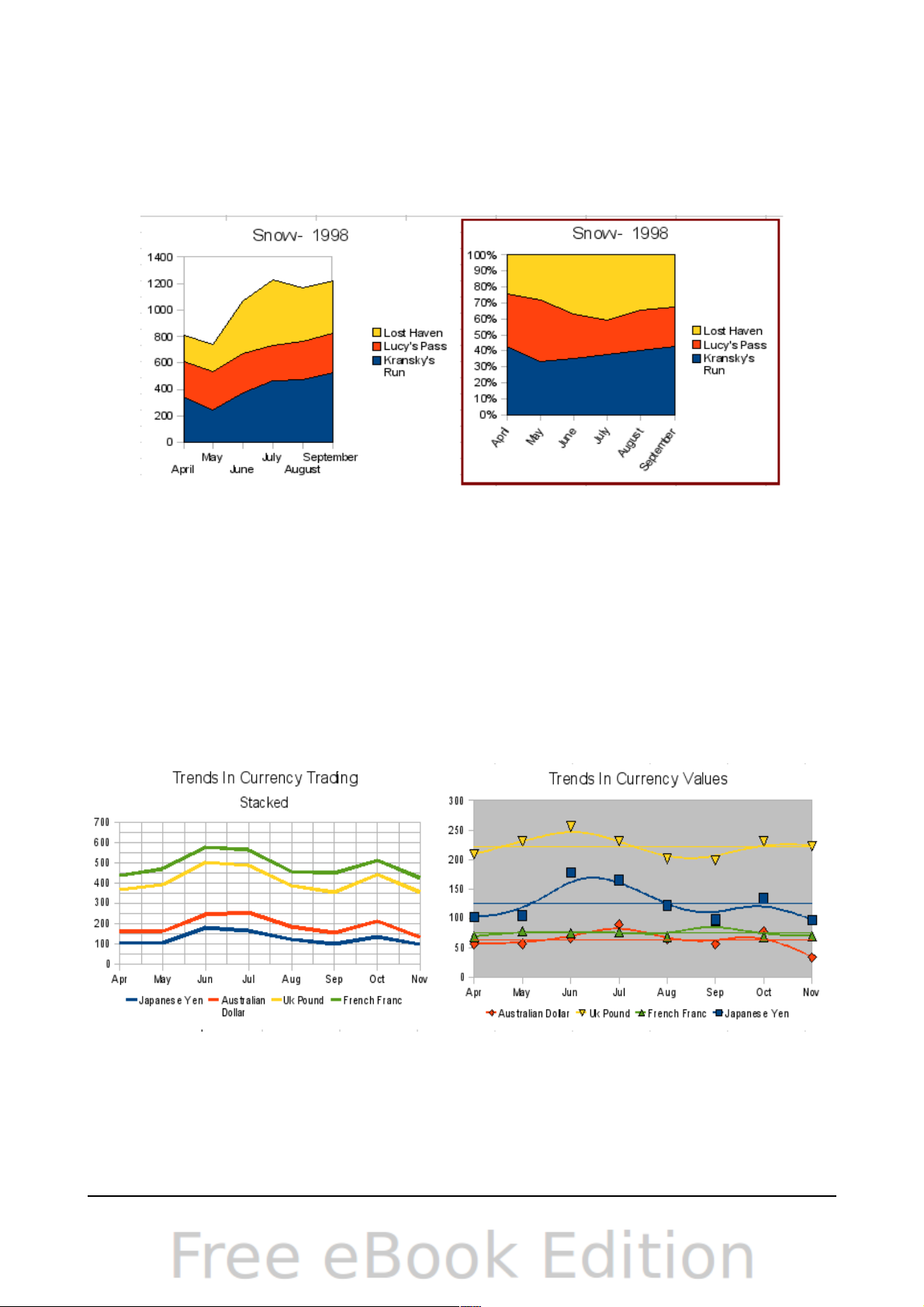
a picture of the sky. As you can see, the legend turns into labels on the z-axis. But overall, though it is visually more appealing, it is more difficult to see the point you are trying to make with the data.

Other ways of visualizing the same data series are represented by the stacked area chart or the percentage stacked area chart.

The first does what it says: each number of each series is added to the others so that it shows an overall volume but not a comparison of the data. The percentage stacked chart shows each value in the series as a part of the whole. For example in June all three values are added together and that number represents 100%. The individual values are a percentage of that. Many charts have varieties which have this option.

Line charts

A line chart is a time series with a progression. It is ideal for raw data, and useful for charts with plentiful data that show trends or changes over time where you want to emphasize continuity. On line charts, the x-axis is ideal to represent time series data.

Scatter or XY charts

Scatter charts are great for visualizing data that you have not had time to analyze, and they may be the best for data when you have a constant value against which to

Chapter 3 Creating Charts and Graphs 93

Figure 88: Stacked and percentage stacked area charts

Figure 89: Line charts

compare other data. Examples of good scatter charts might include weather data, reactions under different acidity levels, conditions at altitude or any data which matches two series of numeric data. In contrast to line charts, the x-axis is to the left of the right labels, which usually indicates a time series.

Scatter charts may surprise those unfamiliar with how they work. While constructing the chart, if you choose Data Range > Data series in rows, the first row of data represents the x-axis. The rest of the rows of data are then compared against the first row data. Figure 90 shows a comparison of three currencies with the Japanese Yen. Even though the table presents the monthly series, the chart does not. In fact the Japanese Yen does not appear; it is merely used as the constant series that all the other data series are compared against.

Bubble charts

A bubble chart is a variation of a scatter chart in which the data points are replaced with bubbles. It shows the relations of three variables in two dimensions. Two variables are used for the position on the X-axis and Y-axis, while the third is shown as the relative size of each bubble. One or more data series can be included in a single chart.

Bubble charts are often used to present financial data. The data series dialog for a bubble chart has an entry to define the data range for the bubbles and their sizes.

94 OpenOffice.org 3.3 Calc Guide

Figure 90: A particularly volatile time in the world currency market.

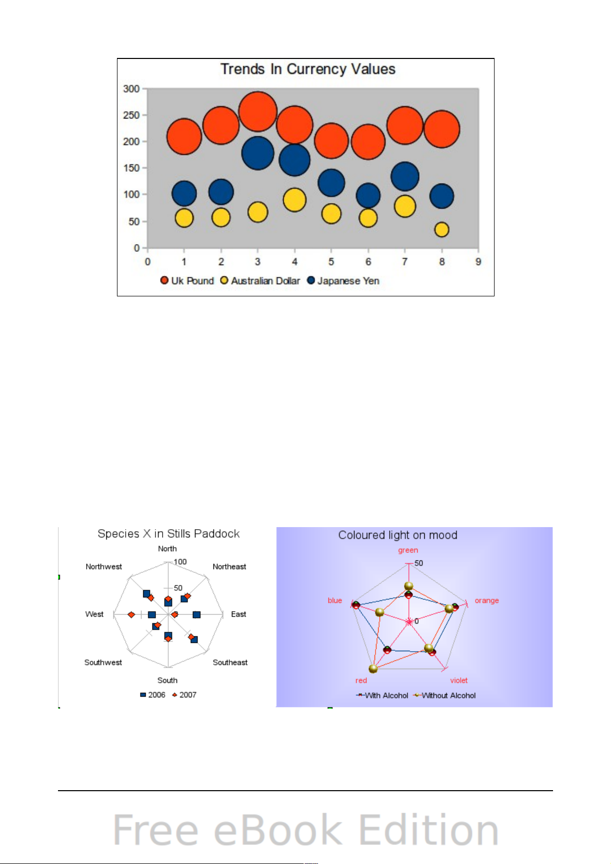
Figure 91: Bubble chart showing three data series

Net charts

A net chart is similar to a polar or radar chart. It is useful for comparing data that is not a time series but shows different circumstances, such as variables in a scientific experiment or direction. The poles of the net chart are equivalent to the y-axes of other charts. Generally, between three and eight axes are best; any more and this type of chart becomes confusing. Before and after values can be plotted on the same chart, or perhaps expected and real results, so that differences can be compared.

Figure 92 shows two types of net charts:

• (Left): A plain net chart without grids or lines, only points.

• (Right): A net chart with lines, points and a grid. Axes colors and labels have

been changed. The chart area color has been changed with a gradient effect. The points on this graph have been changed to fancy 3D spheres.

Chapter 3 Creating Charts and Graphs 95

Figure 92: Two net diagrams showing totally fabricated data from totally fictional experiments.

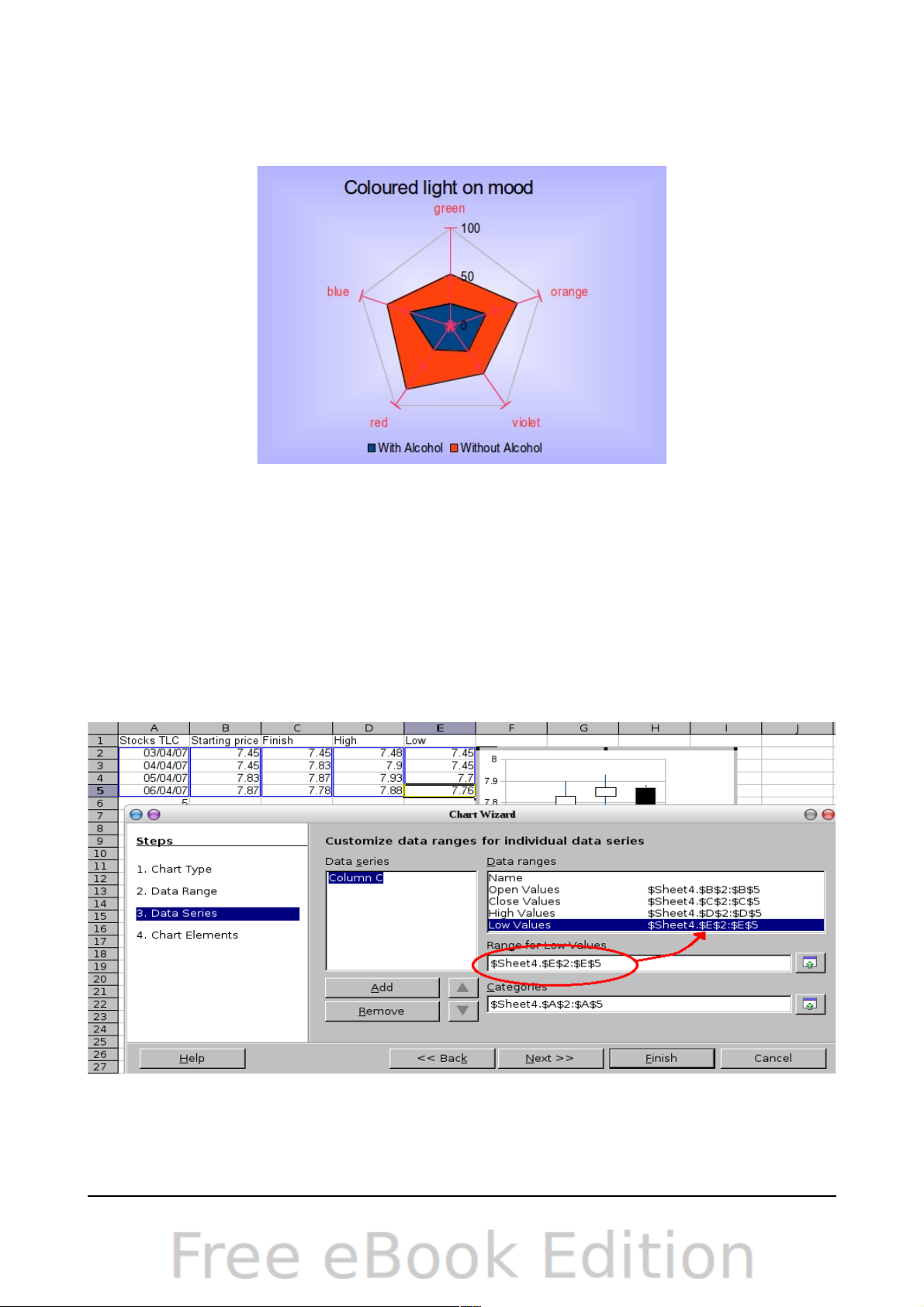
Other varieties of a net chart can be made to show the data series as stacked numbers or stacked percentages. The series can also be filled with a color (Figure

93). Partial transparency is often best for showing all the series all at once.

Stock charts

A stock chart is a specialized column graph specifically for stocks and shares. You can choose traditional lines, candlestick, and two-column type charts. The data required for these charts is quite specialized, with series for opening price, closing price and high and low prices. In this type of chart, the x-axis represents a time series.

When you set up a stock chart in the Chart Wizard, the Data Series dialog is very important. You need to tell it which series represents the opening price, the closing price, the high and low price of the stock, and so on.

A nice touch is that OpenOffice.org stock charts color-code the rising and falling shares: white for rising and black for falling in the candlestick chart and red and blue in the traditional line chart.

96 OpenOffice.org 3.3 Calc Guide

Figure 93: Filled net or radar chart

Figure 94: Adjusting data series for stock charts.

Column and line charts

A column and line chart is a combination of two other chart types. It is useful for combining two distinct but related data series like sales over time (column) with a profit margin trends (line).

You can choose the number of columns and lines in the Chart Wizard. So for example you might have two columns with two lines to represent two product lines with the sales figures and profit margins of both.

The chart in Figure 95 has manufacturing cost and profit data for two products, over a period of time (six months in 2007). To create this chart, first highlight the table and start the Chart Wizard. Choose the Column and Line chart type with two lines and the data series in rows. Then give it a title to highlight the aspect you want to show. The lines are different colors at this stage and don’t reflect the product relationships. When you finish with the Chart Wizard, highlight the chart, click on the line, right-click and chose Format Data Series.

On this tab there are a few things to change: The colors should match the products so both Ark Manufacturing and its profit line are blue and Prall Manufacturing is red. The lines need to be more noticeable so make the lines thicker by increasing the width to 0.08.

For the background, highlight the chart wall, right-click and choose Format Wall. On the Area tab, change the drop-down box to show Gradient. Choose one of the preset gradient patterns and make it lighter by going to the Transparency tab and making the gradient 50% transparent.

To make the chart look cleaner without the grid, go to Insert > Grids and deselect the X-axis option.

Chapter 3 Creating Charts and Graphs 97

Figure 95: Column and line chart

Chapter 4

Using Styles and

Templates in Calc

Bringing uniformity to your spreadsheets

What is a template?

A template is a model that you use to create other documents. For example, you can create a template for invoices that has your company’s logo and address at the top of the page. New spreadsheets created from this template will all have your company’s logo and address on the first page.

Templates can contain anything that regular documents can contain, such as text, graphics, styles, and user-specific setup information such as measurement units, language, the default printer, and toolbar and menu customization.

All documents in OpenOffice.org are based on templates. You can create, or download and install, as many templates as you wish. If you do not specify a template when you start a new a new spreadsheet, the new spreadsheet is based on the default template for spreadsheets. If you have not specified a default template, OOo uses the blank spreadsheet template that is installed with OOo. See “Setting a default template” on page 113.

What are styles?

A style is a set of formats that you can apply to selected elements in a document to quickly change their appearance. When you apply a style, you apply a whole group of formats at the same time.

Many people manually format spreadsheet cells and pages without paying any attention to styles. They are used to formatting documents according to physical attributes. For example, for the contents of a cell you might specify the font family, font size, and any formatting such as bold or italic.

Styles are logical attributes. Using styles means that you stop saying “font size 14pt, Times New Roman, bold, centered”, and you start saying “Title” because you have defined the “Title” style to have those characteristics. In other words, styles means that you shift the emphasis from what the text (or page, or other element) looks like, to what the text is.

Styles help improve consistency in a document and can greatly speed up formatting. They also make major formatting changes easy. For example, you may decide to change the appearance of all subtotals in your spreadsheet to be 10 pt. Arial instead of 8 pt. Times New Roman after you have created a 15-page spreadsheet; you can change all of the subtotals in the document by simply changing the properties for the subtotal style.

Page styles assist with printing, so you don’t need to define margins, headers and footers, and other printing attributes each time you print a spreadsheet.

Types of styles in Calc

While some components of OOo offer many style types, Calc offers only two:

• Cell styles include fonts, alignment, borders, background, number formats (for

example, currency, date, number), and cell protection.

• Page styles include margins, headers and footers, borders and backgrounds,

and the sequence for printing sheets. The page size, orientation, and other attributes of a page style apply only when a spreadsheet is printed; they are not displayed onscreen.

Chapter 4 Using Styles and Templates in Calc 99

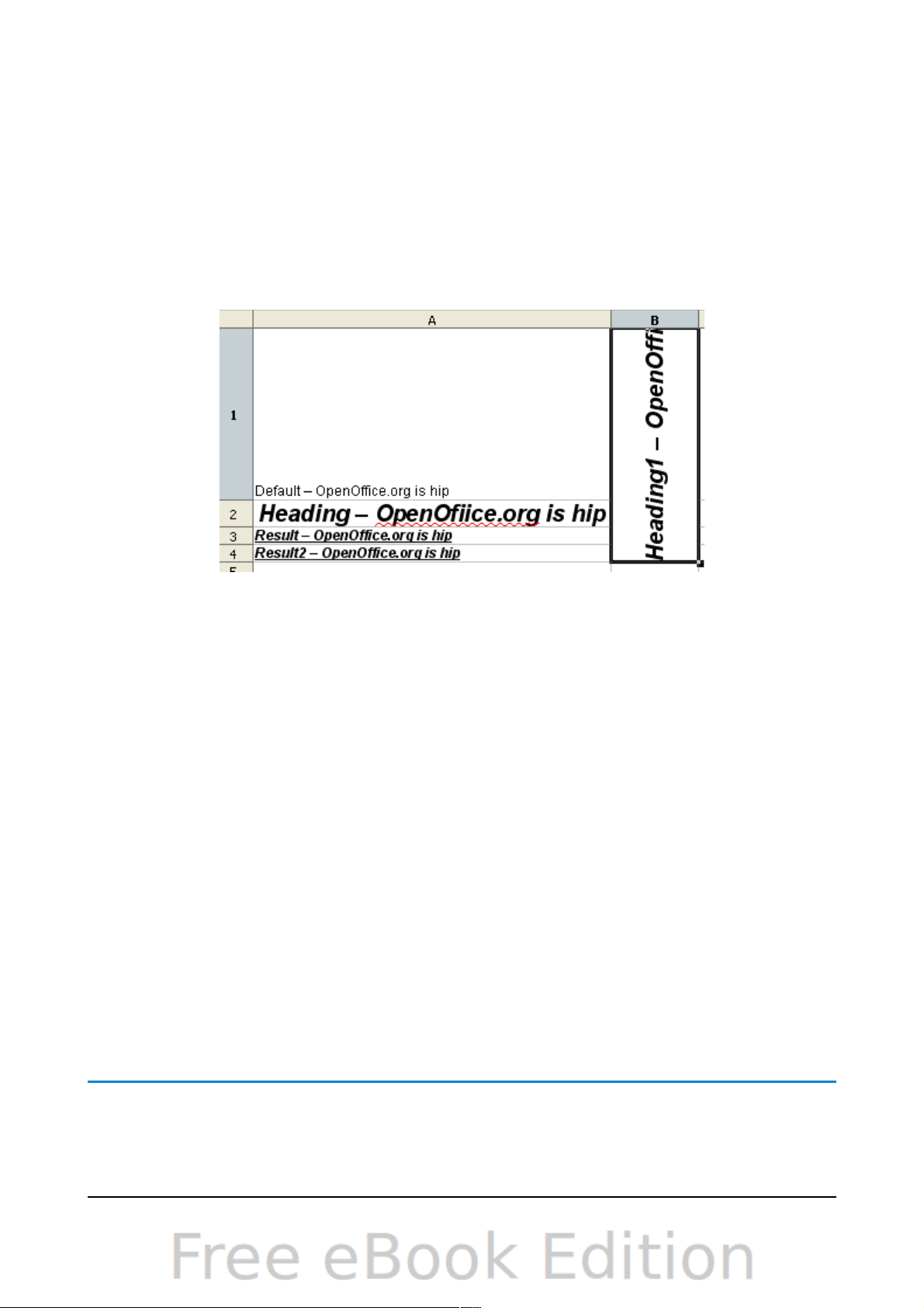
Cell styles

Similar to paragraph styles in OOo Writer, cell styles are the most basic type of style in Calc. You can apply a cell style to a cell and that cell will follow the formatting rules of the style. Five cell styles are supplied with OOo: Default, Heading, Heading1, Result, and Result2.

Initially, the styles are configured so that if you change the font family of Default, then all of the other styles will change to match. We will discuss how to set this up in “Creating new (custom) styles” on page 106. The five standard styles can be seen in use in Figure 96.

Page styles

Page styles in Calc are applied to sheets. Although one sheet may print on several pages (pieces of paper), only one page style can be applied to a sheet. If a spreadsheet file contains more than one sheet, the different sheets can have different page styles applied to them. So, for example, a spreadsheet might contain one sheet to be printed in landscape orientation (using the Default page style) and another sheet to be printed in portrait orientation (using the Report page style).

Two page styles are supplied with Calc: Default and Report. The major difference between these two styles is that Report is portrait-oriented and Default is landscapeoriented. You can adjust many settings using page styles. You can also define as many page styles as you wish.

Because spreadsheets are primarily used onscreen and not printed, Calc does not display the page style on the screen. If you want a spreadsheet to fit on a certain page size, you have to carefully control the column width and row height, with only File > Page Preview to guide you.

Despite this limitation, it’s well worth defining page styles for any spreadsheets that you are likely to print. Otherwise, if a need for printing does arise, you may lose time to trial and error.

Accessing styles

The main way to access styles is through the Styles and Formatting window (shown in Figure 97). You can open this window in several ways.

• Keyboard: Press the F11 key.

100 OpenOffice.org 3.3 Calc Guide

Figure 96: Calc cell style types

OpenOffice 3.3 Calc Guide

Specifications and Main Features

Frequently Asked Questions

User Manual

Copyright

Note for Mac users

Chapter 1 Introducing Calc

What is Calc?

Spreadsheets, sheets, and cells

Parts of the main Calc window

Title bar

Menu bar

Toolbars

Displaying or hiding toolbars

Palettes and tear-off toolbars

Moving toolbars

Docking/floating windows and toolbars

Customizing toolbars

Formatting toolbar

Formula Bar

Right-click (context) menus

Individual cells

Sheet tabs

Status bar

Starting new spreadsheets

Starting a new document from a template

Opening existing spreadsheets

Opening CSV files

Saving spreadsheets

Saving a document automatically

Saving as a Microsoft Excel document

Saving as a CSV file

Saving in other formats

Password protection

Navigating within spreadsheets

Going to a particular cell

Moving from cell to cell

Customizing the effects of the Enter key

Moving from sheet to sheet

Selecting items in a sheet or spreadsheet

Selecting cells

Selecting columns and rows

Selecting sheets

Working with columns and rows

Inserting columns and rows

Deleting columns and rows

Working with sheets

Inserting new sheets

Deleting sheets

Renaming sheets

Viewing Calc

Using Zoom

Freezing rows and columns

Splitting the screen

Splitting the screen horizontally

Splitting the screen vertically

Removing split views

Using the Navigator

Moving quickly through a document

Choosing a drag mode

Using document properties

Chapter 2 Entering, Editing, and Formatting Data

Introduction

Entering data using the keyboard

Entering numbers

Entering text

Entering numbers as text

Entering dates and times

Entering special characters

Inserting dashes

Deactivating automatic changes

Speeding up data entry

Using the Fill tool on cells

Using a fill series

Defining a fill series

Using selection lists

Sharing content between sheets

Validating cell contents

Editing data

Removing data from a cell

Chapter 1

Introducing Calc

Chapter 2

Entering, Editing, and

Formatting Data