

Page 1

SAMM
Stand Alone Mosaicking Module
User Manual
Oceanic Imaging Consultants, Inc.
1144 10th Avenue • Suite 200
Honolulu, Hawai‘i 96816-2442
Phone 808.539.3706 • Fax 808.791.4075
Email support@oicinc.com • Web www.oicinc.com
Page 2

Copyright © 2017 Oceanic Imaging Consultants, Inc. - Printed in the United States of America (USA). All
rights reserved.
This manual and all other related documentation are protected by copyright and distributed under
licenses restricting its use, duplication, distribution, and recompilation. No part of this Manual or related
documentation covered by copyright herein may be reproduced in any form or by means -- graphic,
electronic, or mechanical -- including photocopying, recording, taping, or storage in an information
retrieval system, without the prior written authorization of Oceanic Imaging Consultants, Inc.
The products described in this manual may be protected by one or more U.S. or foreign patents, and
pending applications.
Oceanic Imaging Consultants, Inc. retains the right to make changes to the contents of this Manual at any
time, without notice. Oceanic Imaging Consultants, Inc. makes no warranty for the use of its products
and assumes no responsibility for any errors that may appear in this document, nor does it make a
commitment to update the information contained herein.
Oceanic Imaging Consultants, Inc.
1144 10th Avenue • Suite 200
Honolulu, Hawai‘i 96816-2442
www.oicinc.com
Telephone: 808.539.3706
Fax: 808.539.3710
Email: support@oicinc.com
TRADEMARKS
SAMM is a trademark of Oceanic Imaging Consultants, Inc., in the U.S.A. and other countries.
Third party trademarks are the property of their respective owners and should be treated as such.
WARNING AND DISCLAIMER
Every effort has been made to make this manual as complete and as accurate as possible, but no
warranty or fitness is implied. The information provided is on an “as is” basis. The authors and the
publisher shall have neither liability nor responsibility to any person or entity with respect to any loss or
damages arising from the information contained in this book or from the use of the CD or programs
accompanying it.
Rev. 2/17/2017
Page 3

SAMM User Manual
Table of Contents
1 WELCOME TO SAMM ...................................................................................................... 6
2 SYSTEM REQUIREMENTS AND SETUP......................................................................... 8
2.1 Sensor and Input Requirements ................................................................................................ 8
2.2 System Requirements ............................................................................................................... 9
2.3 Installing SAMM ....................................................................................................................... 10
2.4 Launch SAMM ......................................................................................................................... 11
2.5 Create or Open a Project ......................................................................................................... 12
3 THE GRAPHICAL USER INTERFACE ............................................................................14
3.1 Mosaic Window ....................................................................................................................... 14
3.2 Toolbar ..................................................................................................................................... 15
3.3 Sidebar .................................................................................................................................... 16
3.3.1 Swath List ...................................................................................................... 17
3.3.2 Live Info ......................................................................................................... 17
3.3.3 Playback Controls .......................................................................................... 17
3.3.4 Sonar Controls ............................................................................................... 18
3.3.5 Processing Controls ...................................................................................... 18
3.4 Forward Look Window ............................................................................................................. 19
3.5 SLS Oscilloscope Window ....................................................................................................... 19
3.6 Meta Data Properties ............................................................................................................... 20
3.7 Status Bar ................................................................................................................................ 20
4 CONFIGURE SAMM ........................................................................................................22
4.1 Project Tab .............................................................................................................................. 23
4.1.1 Projected Coordinate System ........................................................................ 23
4.1.2 Sensor Offsets ............................................................................................... 23
4.2 Display Tab .............................................................................................................................. 24
4.2.1 General .......................................................................................................... 24
4.2.2 Swath Colormap ............................................................................................ 25
4.2.3 Units of measure ........................................................................................... 25
4.3 Mosaic Tab .............................................................................................................................. 26
4.3.1 General .......................................................................................................... 26
4.3.2 MSK output (connected/live sonars) ............................................................. 27
4.4 Contacts tab............................................................................................................................. 27
4.5 About ....................................................................................................................................... 28
4.6 Rendering Method ................................................................................................................... 28
4.7 Reset Button ............................................................................................................................ 29
4.8 Configuration Tutorial .............................................................................................................. 29
5 CHARTS AND BACKGROUND IMAGES ........................................................................31
5.1 Basic vs. Advanced Interface .................................................................................................. 31
5.2 Raster vs. Vector File Types ................................................................................................... 31
5.3 Retrieve NOAA Electronic Navigational Charts ....................................................................... 31
5.4 Elements of the Basic Chart Display Options Window ............................................................ 32
5.4.1 Basic Chart Display Popup Windows ............................................................ 33
5.4.2 Using the Basic Chart Loader ....................................................................... 34
5.5 Elements of the Advanced Chart Display Options Window .................................................... 35
5.5.1 Buttons .......................................................................................................... 36
5.5.2 The Folders Tab ............................................................................................ 37
Populating the Charts Database ................................................................... 37
5.5.3 The Chart Preview Tab.................................................................................. 38
5.5.4 The Charts Tab .............................................................................................. 39
5.5.4.1 Color Coding .................................................................................................. 39
Green ............................................................................................................. 40
1
Page 4

SAMM User Manual
Orange ........................................................................................................... 40
Yellow ............................................................................................................ 40
Gray ............................................................................................................... 40
Manually Loaded vs. Folder Added Chart Behavior ...................................... 40
5.5.5 The Log Tab .................................................................................................. 41
5.6 Advanced Chart Loader Tutorial ............................................................................................. 41
5.7 Chart Customization Commands............................................................................................. 41
6 ADD FILES OR BEGIN ACQUISITION ............................................................................43
6.1 Add Files in Playback or Post-Processing Mode ..................................................................... 43
6.1.1 Load Files ...................................................................................................... 43
6.1.2 Advanced Load Files ..................................................................................... 44
6.1.3 Playback Files ............................................................................................... 45
6.1.4 Advanced Playback Files .............................................................................. 45
6.2 Load Files from Directory ........................................................................................................ 47
6.3 Interface with Metadata Sensors ............................................................................................. 49
6.4 Connect To…........................................................................................................................... 50
6.4.1 Kongsberg Mesotech M3 .............................................................................. 50
6.4.2 Kongsberg Mesotech MS1000 ...................................................................... 51
6.4.3 Teledyne BlueView 2D Multibeam Imaging Sonar ........................................ 52
6.4.4 Tritech Gemini 720i/is, Marine Electronics Dolphin, Blueprint Oculus, or
R2Sonic ...................................................................................................................... 54
Troubleshooting ............................................................................................. 54
Gemini Sonar Controls .................................................................................. 55
R2Sonic Sonar Controls ................................................................................ 56
Marine Electronics Dolphin Sea View ........................................................... 57
6.4.5 Edgetech Discover, Klein SonarPro and GeoDAS ........................................ 59
Edgetech Discover ........................................................................................ 59
Klein SonarPro .............................................................................................. 60
GeoDAS ........................................................................................................ 61
7 DISPLAY AND PROCESSING SETTINGS ......................................................................63
7.1 Adjust the Mosaic Window Display.......................................................................................... 63
7.2 Manage Swaths ....................................................................................................................... 64
7.2.1 Swath Management and Playback Tutorial ................................................... 64
7.3 Toggle Display Units ................................................................................................................ 65
7.3.1 Display Units Tutorial ..................................................................................... 65
7.4 Apply Imagery Processing Options ......................................................................................... 66
7.4.1 Processing Controls ...................................................................................... 66
7.4.2 Swath Properties ........................................................................................... 67
7.4.3 Playback of *.son files ................................................................................... 67
7.5 Other Display Options ............................................................................................................. 68
7.6 Imagery Processing Tutorials .................................................................................................. 69
Trimming Tutorial ........................................................................................... 69
Rendering Tutorial ......................................................................................... 69
8 WORKING WITH CONTACTS .........................................................................................72
8.1 Mark Contacts.......................................................................................................................... 72
8.2 Elements of the Contacts Window........................................................................................... 73
8.2.1 Thumbnails List ............................................................................................. 74
8.2.2 Contacts Toolbar ........................................................................................... 74
8.2.3 Contact Display ............................................................................................. 75
8.2.4 Properties Table ............................................................................................ 75
8.2.5 Staging Table ................................................................................................ 75
8.2.6 Contact Display Commands .......................................................................... 76
8.3 Attribute Contacts .................................................................................................................... 77
8.3.1 Classify Contacts ........................................................................................... 78
2
Page 5

SAMM User Manual
Add Comments .............................................................................................. 78
Add Tags ....................................................................................................... 78
8.3.2 Measure Contacts ......................................................................................... 79
8.3.3 Calculate Contact Height ............................................................................... 79
8.3.4 Change Position ............................................................................................ 79
8.3.5 Rename Contacts .......................................................................................... 79
8.3.6 Contact Attribution Commands ..................................................................... 80
8.4 Group Contacts ....................................................................................................................... 81
8.5 Export Contacts ....................................................................................................................... 82
8.5.1 Send contacts to the staging table ................................................................ 82
8.5.2 Prep the Staging Table .................................................................................. 83
8.5.3 Export a Report ............................................................................................. 83
8.5.4 Delete Contacts ............................................................................................. 84
8.5.5 Contact Organization Commands ................................................................. 84
8.6 Contacts Tutorial ..................................................................................................................... 85
9 ADDITIONAL FEATURES ...............................................................................................88
9.1 Meta data properties ................................................................................................................ 88
9.2 Select tool ................................................................................................................................ 88
9.3 Measure tool ............................................................................................................................ 88
9.4 Export Tool .............................................................................................................................. 89
9.4.1 File Type ........................................................................................................ 90
9.4.2 Extents ........................................................................................................... 91
9.4.3 Resolution ...................................................................................................... 91
9.4.4 Background color ........................................................................................... 91
9.4.5 Export Tutorial ............................................................................................... 91
10 END ACQUISITION AND CLOSE PROJECT ..................................................................92
Figures
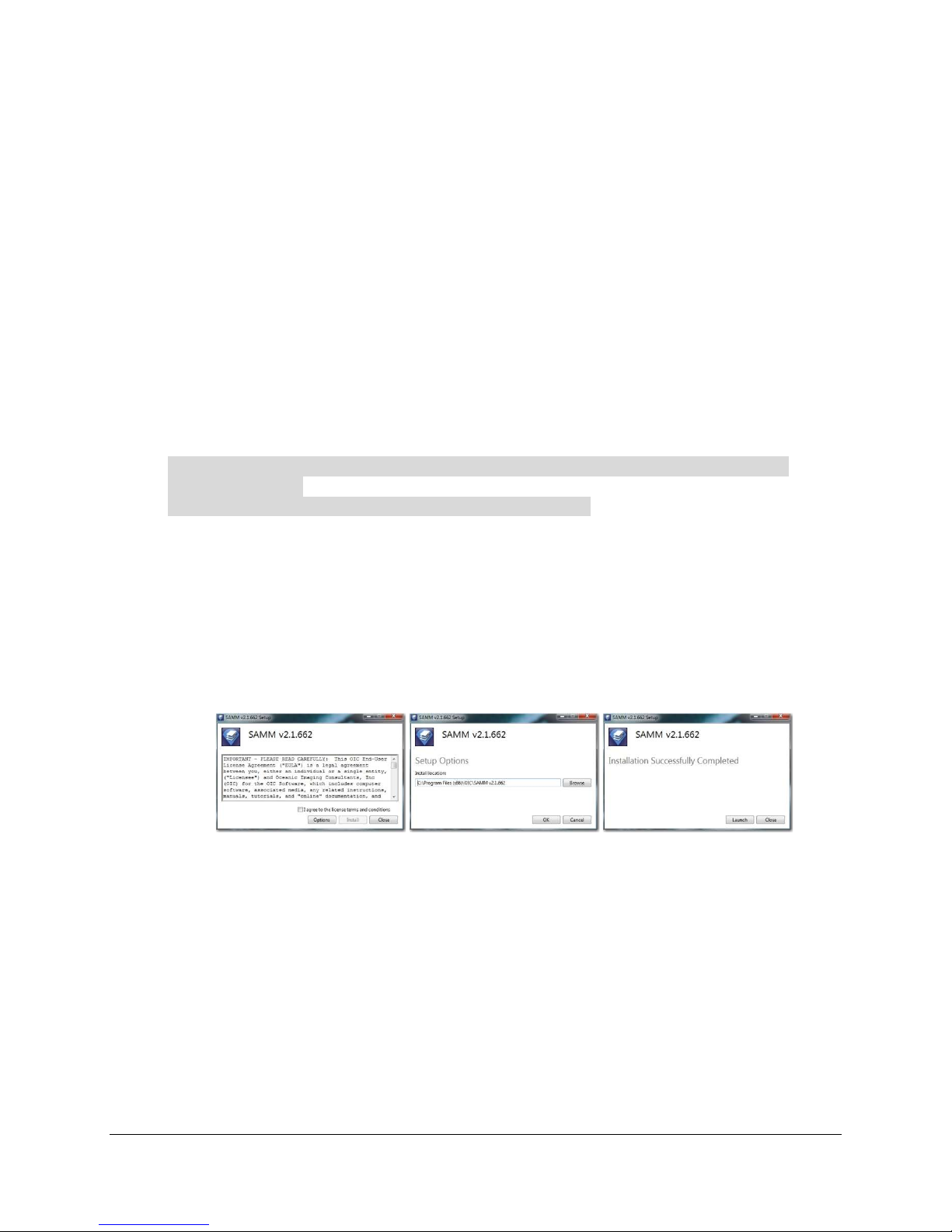
Figure 1. SAMM installation process and dialogs ....................................................................................... 10
Figure 2. SAMM opening dialog, allowing creation of new project, opening existing or mission import. ... 12
Figure 3. Graphical User Interface .............................................................................................................. 14
Figure 4. Swath List .................................................................................................................................... 17
Figure 5. Live Info ....................................................................................................................................... 17
Figure 6. Playback Controls ........................................................................................................................ 17
Figure 7. Sonar Controls ............................................................................................................................. 18
Figure 8. FLS Controls ................................................................................................................................ 18
Figure 9. SLS Controls ................................................................................................................................ 18
Figure 10. Forward Look Window ............................................................................................................... 19
Figure 11. SLS Oscilloscope Window ......................................................................................................... 19
Figure 12. Meta Data Properties ................................................................................................................. 20
Figure 13. Configuration Dialog .................................................................................................................. 22
Figure 14. Projection Tab ............................................................................................................................ 22
Figure 15. Survey Setup Panel ................................................................................................................... 24
Figure 16. General Panel ............................................................................................................................ 25
Figure 17. Swath Colormap Panel .............................................................................................................. 25
Figure 18. Units of Measure Panel ............................................................................................................ 25
Figure 19. General Panel ............................................................................................................................ 26
Figure 20. MSK output Panel ...................................................................................................................... 27
Figure 21. Contacts Tab ............................................................................................................................. 27
Figure 22. About Panel ............................................................................................................................... 28
Figure 23. Update Panel ............................................................................................................................. 28
Figure 24. Crash Detection Prompt ............................................................................................................ 28
3
Page 6

SAMM User Manual
Figure 25. Configuration Window for Demo Data ....................................................................................... 30
Figure 26. Empty Basic Chart Display Options Window ............................................................................. 32
Figure 27. Select Overlay Type Error Message .......................................................................................... 33
Figure 28. ASCII Text Import Options ......................................................................................................... 34
Figure 29. Charts Loaded in Basic Window, with Context Menu................................................................ 34
Figure 30. Chart Display Options Window upon Launch ............................................................................ 36
Figure 31. Add/Scan Charts Panel ............................................................................................................. 37
Figure 32. Populated Chart Database ........................................................................................................ 38
Figure 33. Charts Tab ................................................................................................................................. 39
Figure 34. Add Data Dropdown Menu ........................................................................................................ 43
Figure 35. Advanced Load Dialog .............................................................................................................. 44
Figure 36. Advanced Playback Dialog ........................................................................................................ 46
Figure 37. GUI in Playback Mode ............................................................................................................... 47
Figure 38. Load from directory dialog ......................................................................................................... 48
Figure 39. Navigation Interfacing ................................................................................................................ 49
Figure 40. M3 Interfacing ............................................................................................................................ 50
Figure 41. MS1000 Interfacing.................................................................................................................... 51
Figure 42. ProViewer NMEA Panel ............................................................................................................ 52
Figure 43. ProViewer Data Streaming Configuration ................................................................................. 52
Figure 44. BlueView Interfacing .................................................................................................................. 53
Figure 45. Gemini Interfacing...................................................................................................................... 54
Figure 46. Gemini Sonar Controls .............................................................................................................. 55
Figure 47. Black banding artifacts with high gain and the same data with lower gain. .............................. 56
Figure 48. R2Sonic Sonar Controls ............................................................................................................ 56
Figure 49. Dolphin Sea View Interfacing .................................................................................................... 57
Figure 50. Dolphin Sea View Controls ........................................................................................................ 57
Figure 51. Blueprint Oculus Interfacing ...................................................................................................... 58
Figure 52. Blueprint Oculus Controls .......................................................................................................... 58
Figure 53. SAMM interface to Edgetech Discover ..................................................................................... 59
Figure 54. SAMM interface to Klein SonarPro ............................................................................................ 60
Figure 55. GeoDAS UDP Broadcast Settings ............................................................................................. 61
Figure 56. SAMM Interface to GeoDAS ...................................................................................................... 61
Figure 57. Status Bar Position Units ........................................................................................................... 66
Figure 58. Imagery Processing Options ..................................................................................................... 66
Figure 59. SLS Processing Options ............................................................................................................ 67
Figure 60. Swath Properties Window ......................................................................................................... 67
Figure 61. Display Options Dialog With Navigation Track Options ............................................................ 68
Figure 62. Brightness and Gamma Rendering Effects ............................................................................... 70
Figure 63. Feathering Effect ....................................................................................................................... 70
Figure 64. Contacts in Mosaic Window ...................................................................................................... 72
Figure 65. Contacts Window ....................................................................................................................... 73
Figure 66. Assigning Tags .......................................................................................................................... 79
Figure 67. Grouped Contacts and Context Menu ....................................................................................... 82
Figure 68. Filtering by Tag .......................................................................................................................... 83
Figure 69. Create Report Success Window ................................................................................................ 84
Figure 70. Meta data properties window ..................................................................................................... 88
Figure 71. Measure Tool ............................................................................................................................. 89
Figure 72. Export dialog .............................................................................................................................. 89
Figure 73. Single GeoTIFF export vs Tiled GeoTIFFs export .................................................................... 90
Figure 74. Exported data displayed in GoogleEarth ................................................................................... 90
4
Page 7

SAMM User Manual
Tables
Table 1. System Requirements ................................................................................................................ 9
Table 2. Create or Open Project ................................................................................................................. 13
Table 3. Toolbar Icons ................................................................................................................................ 15
Table 4. Status bar ...................................................................................................................................... 20
Table 5. Parameters and Units ................................................................................................................... 26
Table 6. Change the Rendering Method ..................................................................................................... 29
Table 7. Configure Project .......................................................................................................................... 29
Table 8. Load and Display Charts............................................................................................................... 41
Table 9. Chart Customization Commands .................................................................................................. 41
Table 10. Mosaic Window Extent Commands ............................................................................................ 63
Table 11. Swath Management Commands ................................................................................................ 64
Table 12. Contacts Toolbar Icons ............................................................................................................... 74
Table 13. Contact Display Commands ....................................................................................................... 76
Table 14. Contact Attribution Commands ................................................................................................... 80
Table 15. Contact Organization Commands ............................................................................................... 84
Acronyms and Abbreviations
cm centimeter
CPU central processing unit
ENC Electronic Navigational Chart
FLS forward-looking sonar
GIS geographic information system
GPU graphics processing unit
GUI graphical user interface
NMEA National Marine Electronics Association
NOAA National Oceanic and Atmospheric Administration
OIC Oceanic Imaging Consultants, Inc.
PPI plan position indicator
SAMM Stand Alone Mosaicking Module
SLS
TIFF
UTM Universal Transverse Mercator
side-looking sonar
Tagged-Image File Format
5
Page 8

SAMM User Manual
1 Welcome to SAMM
There was a time not too long ago when the interface to a sonar was a printer. The sonar would
ping, echoes would return, be converted to voltage, and a stylus on a moving belt would cross a
scroll of paper, burning images proportional to the echo strength. Now many sonars come with
perfectly adequate graphical user interfaces that create a waterfall or PPI (plan-position
indicator) view of the data. These are fine, but often lack context, i.e. they don’t show the data
in reference to each other, or the world. SAMM changes all this.
SAMM (Stand Alone Mosaicking Module) is Oceanic Imaging Consultants Inc.’s (OIC) software
program for real-time mosaicking of underwater imagery. SAMM automatically creates mosaics
of your sidescan, forward-look (FLS) and mechanical scanning sonar data in real time over your
co-registered charts or imagery, while logging the raw data for playback and post-processing.
Whether in real-time or playback, SAMM will show where you’ve been and what you saw.
This manual documents SAMM’s features and functions. Information is presented in the order
that you need it for out-of-the-box playback or data acquisition. It discusses each process in the
SAMM workflow and how to accomplish it. Selected sections conclude with a table of
commands relevant to the workflow process described in that section, which serves as a review
of the commands available in SAMM and how to execute them. Selected sections also include
an interactive tutorial for demonstrating some of the features. Test data are provided with the
software for use with the tutorial instructions. The sections are as follows:
System Requirements and Setup
The Graphical User Interface (GUI)
Configure SAMM
Load Charts
Add Files or Begin Acquisition
Display and Processing Settings
Work with Contacts
Additional Features
End Acquisition and Close Project.
We use the following typographical rules throughout this manual for emphasis and clarity:
Boldface indicates onscreen buttons, commands, fields, or icons from a toolbar, menu
or window.
Courier New indicates user input or SAMM output. This includes all of the text in the
SAMM interface that your actions can change.
Grey shading of text or columns in a table indicates specific tutorial instructions. Follow
these directions to check your work against the figures in this manual.
Key names are written as they appear on the keyboard. Key combinations are indicated
with a plus sign between them, e.g., to press Alt+F, press Alt and F simultaneously.
Click means to press the left mouse button. Double-click means to quickly press the left
mouse button twice. Right-click means to press the right mouse button.
For further assistance using the SAMM program, we encourage you to contact us.
Phone 1-808-539-3706 Fax: 1-808-539-3710
e-mail support@oicinc.com Web: www.oicinc.com
6
Page 9

SAMM User Manual
7
Page 10

SAMM User Manual
2 System Requirements and Setup
This section describes the sensor and system requirements for computers hosting SAMM, and
how to install, launch, and create/open a project in the software.
2.1 Sensor and Input Requirements
SAMM is designed to read sonar data, position and sensor heading, and produce a mosaic.
SAMM can do this for forward-look, sector-scan and side-look (sidescan) sonars. SAMM can
read this data in real-time from the sensor, or from files in playback mode. In forward-look
mode, SAMM is compatible with Kongsberg Mesotech M3, Teledyne BlueView 2D imaging,
Tritech Gemini, Marine Electronics Dolphin SeaView, Blueprint Subsea Oculus, Haiying Marine
HY1645 and the R2Sonic 202x in forward-looking mode. SAMM can also interface with
Kongsberg Mesotech MS1000 single-beam scanning sonar and Imagenex 881L-GS/882L gyro
stabilized scanning sonar. In sidescan mode, SAMM is compatible with Edgetech Discover (and
all supported sonars), Klein SonarPro (and all supported sonars) and OIC’s GeoDAS (and all
supported sonars), SAMM also supports reading of Starfish .logdoc, Triton .xtf, C-Max .cm2,
and Humminbird .dat data. Contact OIC for other sonar formats. SAMM requires input of
sensor position (longitude/latitude) as well as true heading. SAMM assumes your GPS receiver
is set to the WGS 1984 reference datum, but supports user configuration of datum.
SAMM directly interfaces to the Tritech Gemini 720, the R2Sonic 202x, the Marine Electronics
Dolphin SeaView and the Blueprint Subsea Oculus FLS, effectively replacing any native sonar
software and providing all control, display and logging functions. For these sonars, SAMM
requires:
the sonar software not be run concurrently with SAMM; and
navigation and heading sensors must be supplied to SAMM directly, as they will not be
included with the sonar data
For the sidescan systems (Edgetech, Klein, OIC) and the Kongsberg M3/MS1000, BlueView,
Imagenex 881L-GS/882L and HY1645 sonars, SAMM interfaces with the manufacture's
software, leaving all control and processing to the native sonar software, and providing display,
target marking and mosaicking capabilities. For these sonars, SAMM requires:
the sonar software must be run concurrently with and connected to SAMM; and
navigation and heading sensors or must be supplied to the sonar software, so that
SAMM can receive position and heading included with the sonar data
At the time of this writing, SAMM does not interface in real-time to Sound Metrics ARIS/DIDSON
sonar, Reson 7128/7130 and Norbit forward-looking sonar systems. However, their recorded
data files (.aris/.dds and .s7k) can be loaded or played back in SAMM to generate mosaic
imagery if they are logged with position and heading data.
8
Page 11

SAMM User Manual
Component
Minimum
Recommended
2.2 System Requirements
SAMM is a Windows-based application and compatible with Windows Vista through Windows
10 . The minimum system requirements and recommended specifications are presented in
Table 1.
Table 1. System Requirements
Processor Dual core Quad core
RAM 2 GB 4 GB
Graphics CPU OpenGL 3.1+ compatible GPU and up-to-date
video driver
Display 1024x758 (32 bit color)
Disk Space Install is approximately 300MB, but more space is needed for logging data.
Please be aware that some systems may log close to 1 GB/min.
Ports USB port for dongle;, Ethernet port for sonar connection and serial port(s) if
using NMEA inputs
The computer that is running SAMM does not require a dedicated graphics processing unit
(GPU), but a GPU does provide better performance. SAMM will automatically offload
computation-intensive tasks such as mosaicking and high-quality rendering to the GPU when
the GPU supports OpenGL 3.1+. In practice, most recent Intel central processing units (CPU)
come with an integrated GPU that meets this requirement, as well as most recent
mobile/desktop GPUs from AMD/NVIDIA. You must keep your video driver updated, however.
To ensure that you have the most updated driver for your system, please go to the
manufacturer's Web site:
For AMD/ATI:
http://support.amd.com/en-us/download
For NVIDIA:
http://www.nvidia.com/Download/index.aspx
For Intel HD 3000/4000/5000 series:
https://downloadcenter.intel.com/
In order to run the SAMM software, an OIC-provided dongle must be attached to the
workstation, with up-to-date dongle drivers installed. Dongle drivers are present in the
installation media provided by OIC (see Section 2.3).
9
Page 12
SAMM User Manual
2.3 Installing SAMM
SAMM installs by default to an OIC folder in the Program Files(x86) folder on the local drive.
The installation package comes with a dongle, which looks like a USB stick, and a disc including
three folders: demo_data, documentation, and install. The demo_data folder contains charts, a
demo project, and demo data files in the native SAMM format. The documentation folder
contains the playback tutorial, acquisition tutorial, and this user manual. The install folder
contains the installation file. If you do not have an optical drive on your computer, the
downloadable installation package can be provided over the Web, or via USB drive. Please
contact OIC if you prefer this option.
If you have a limited feature demonstration version, the demo_data folder may contain
additional folders for different sensor data. The limited feature version only plays the included
data files, does not need a dongle to run, and cannot acquire data.
To install SAMM:
1. Put the disc in your disc drive and navigate to the install folder.
2. Create a folder on your local (C:) drive named SAMM_DEMO, for continuity with OIC
training materials.
3. Copy the demo_data folder to the SAMM_DEMO folder. SAMM performs better when
data are saved locally.
4. Insert the OIC dongle into a USB port.
5. Double-click on SAMM-2.x.xxx.exe (file name is not exact).
6. SAMM will present you with the licensing terms agreement page. To accept the terms
and default installation directory, check the “I agree…” statement, and select “ACCEPT”.
To configure installation directory other than the default location, select the “Options”
button. The Setup Options dialog, shown center below, allows you to specify an
alternative installation location. Select “OK” when satisfied or “Cancel” to return. On
successful installation SAMM will inform you of success and offer to launch the software.
Select “Launch” or “Close”
Figure 1. SAMM installation process and dialogs
First time users will also be presented with a language selection dialog, SAMM is currently
available in English and Japanese. Additional language support is being developed. Please
contact OIC for details.
10
Page 13

SAMM User Manual
2.4 Launch SAMM
SAMM launches using standard Window commands, except for the dongle. The dongle must be
in a USB port or you will receive an error message. After securing the dongle, either:
double-click on the SAMM desktop icon;
from Windows Explorer, navigate to the install folder in the Program Files folder, and
double-click on the SAMM.exe; or
click on the Start Windows icon, click on the Oceanic Imaging Consultants folder in All
Programs, then click on the program folder, and finally click on SAMM.
If SAMM has detected multiple crashes, it may present you with the option of switching to
software mode upon launch. You might find it beneficial to test if SAMM performs better in
software mode on your system. SAMM also presents you with the option of sending a crash
detection report if the software crashes. Please fill out this report if you would like our
developers to investigate the cause of your crash.
SAMM comes in English or Japanese. Upon launch, pick the desired language from the
dropdown menu. This dialog only displays on first launch, or when reset from the Configuration
window (see Section 4.7).
11
Page 14
SAMM User Manual
2.5 Create or Open a Project
A SAMM project is a working directory that stores files for the program such as contacts, cached
files, raw data and processed swath and mosaic data. The project folder contains results
obtained from mosaicking the project data, including swath files and exported mosaic data (you
may choose to save exports elsewhere).
The project folder is stored in the workspace, or working directory. For continuity with OIC
training materials, we suggest that you use the SAMM_DEMO folder that you copied the data to
earlier. The default directory is <my documents>\samm_projects, which works just as well. If
you do not choose one of these locations, choose another location, but not one in which you
have installed SAMM executables (i,e., other than C:\Program Files\OIC).
Upon launching OIC's SAMM, choose between creating a new project or opening an existing
project in the select project window (Figure 2).
Figure 2. SAMM opening dialog, allowing creation of new project, opening existing or mission import.
12
Page 15
SAMM User Manual
New project
Open
existing
Recent
projects
Follow the instructions in Table 2 to create a new project or open an existing project. Note that
the “Mission Analysis” option allows one to open a “mission package” consisting of sonar,
camera, chart, navigation and waypoint data and create a SAMM project for this data in post
mission analysis (PMA) mode. For details on Mission Analysis please see Appendix A, “Mission
Analysis”.
At the end of this process, you should have the SAM GUI open, either ready to acquire, load or
playback data, review an existing project or perform post-mission data analysis.
Table 2. Create or Open Project
To create a new project: To open an existing project: To open a recent existing
project:
1. Click
2. Click Browse path... to
open the Select Folder
window.
3. Enter a name in the
Name field: Test.
4. Change the workspace to
C:\SAMM_DEMO
5. Click Create. SAMM's
GUI displays.
tab.
1. Click
project... to open the Open
window.
2. Navigate to the location
where the project is saved
(C:\SAMM_DEMO
\demo_data\Gemini_HawaiiK
ai).
3. Click the geomosaic.xml file
to select it.
4. Click Open. SAMM's GUI
displays.
1. Click
tab.
2. Click the project name.
SAMM's GUI displays.
OR
1. Enter the name of the
project in the Name field
in the New project tab.
2. Click click to open.
SAMM's GUI displays.
13
Page 16
SAMM User Manual
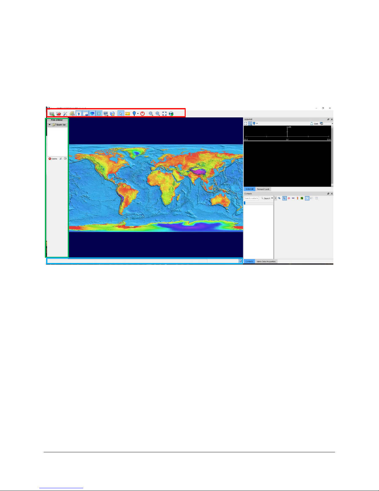
Toolbar
Side
Status Bar
Mosaic Window
Waterfall
Window
Contacts
Window
3 The Graphical User Interface
Before viewing or acquiring data, take a moment to familiarize yourself with the SAMM GUI
(Figure 3). The SAMM interface has a main toolbar, a mosaic window, a status bar, and
ancillary windows with controls which will appear in the sidebar. Some elements are specific to
the acquisition or playback modes. Each element of the GUI is described in a section below.
bar
Figure 3. Graphical User Interface
3.1 Mosaic Window
The multilayer interactive mosaic window shows a geocoded graphic of the geocoded data, plus
any loaded background charts and images. SAMM layers processed sonar data over a
background (navigational chart or aerial imagery) as raw data are collected or loaded. Sections
of the survey track that have been processed from the raw data are referred to as swaths. All of
the swaths from a survey are referred to as the mosaic, or the processed dataset. The
procedure of drawing the swaths in the mosaic window is called mosaicking the swaths. SAMM
only logs or records data when in acquisition mode, not in playback mode, but mosaics swaths
in both acquisition and playback mode.
In playback and acquisition mode, a green outlined polygon represents the vessel. For
sidescan systems the scan should appear to either side of the vessel, adjusted for any offsets.
For forward look systems a section of the sonar data shown in the plan position indicator (PPI)
will appear. The PPI is a pie-shaped “flashlight” view of the sonar data, also found in the
Forward Look window. Pink outlined crosshairs represent the positions of the GPS antenna and
the sonar head.
To see the vessel, data, GPS and sonar head positions, zoom out by rolling your mouse
wheel toward you, clicking the Zoom out icon on the toolbar, pressing the - key, or using
a two finger scroll away from you on a laptop track pad.
14
Page 17

SAMM User Manual
Icon
Icon Name
Function
3.2 Toolbar
The toolbar is a collection of icons that open dialog boxes or directly execute commands when
clicked. The toolbar icons are pictured and described in Table 3. Toolbar Icons, in the order that
they appear from left to right on the toolbar.
Table 3. Toolbar Icons
Add data Displays the dropdown Add Data menu
Close project Closes the current project
Configuration Opens Configuration window
Export
Contacts Opens Contacts window
Metadata
properties
Display the
forward look
window
Display the
sidelook waterfall
window
Display options Displays the dropdown swath display options
Chart
background
options
Record toggle Begins or ends raw data recording to file in acquisition
New swath Breaks mosaicking without pause in acquisition or playback
Opens Export Data window
Opens Metadata Properties window (only available in
playback/acquisition mode)
Opens the Forward Look window
Opens the Sidelook Waterfall window
Opens the Chart Display Options dialog box
mode or mosaicking in playback mode
mode
Select tool Allows user to select swaths or contact markers in the
Measure tool Activates the measure tool
Mark contact tool Activates the mark contact tool
mosaic window
15
Page 18
SAMM User Manual
Mission tools Opens the Kenautics Mission Tool window
Zoom in Zooms in to the center of the mosaic window
Zoom out Zooms out from the center of the mosaic window
Reset the view to
the entire survey
GoTo button Launches the Go To Dialog, allowing users to specify a
Auto adjust the
display to follow
the sensor
Resets the mosaic view to the entire survey
starting location on a map, and zoom in. Used in mission
planning mode.
Automatically centers the mosaic view on the sensor
3.3 Sidebar
The sidebar appears by default to the left of the SAMM mosaic window. It contains various
panels depending on the mode, and can be minimized by clicking the “Hide sidebar” button.
16
Page 19

SAMM User Manual
S
wath
list
Playback controls
3.3.1 Swath List
The
the survey or playback progresses, SAMM lists swaths by
name in this list and paints them in the mosaic window. The
user can enable or disables swaths to show or hide, and reorder them. Section 7.2 describes how to use this list to
manage swaths.
To hide the Swath list, click the Swath list title bar.
Figure 4. Swath List
3.3.2 Live Info
The Live info panel, visible during acquisition and
playback,displays continuously updated values for date,
time, position, heading, and if available, altitude, sound
velocity, and time synchronization (a real-time estimation of
navigation latency). These metadata appear on the sidebar
in playback and acquisition mode (Figure 5). SAMM
retrieves these metadata feeds from the sonar software or
navigation/heading sources (depending on your survey
setup). Time synchronization is computed by SAMM.
Figure 5. Live Info
3.3.3 Playback Controls
appear on the sidebar in playback
mode. The playback controls include a start/pause button
and a slider bar to speed up or slow down playback (Figure
6). Playback of *.son (BlueView data) files includes a Sound
Velocity input box to allow user to change the sound velocity
value with which the data are presented.
To hide the controls, click the Playback controls
icon.
To hide the metadata, click the Live info title bar.
lists the swaths in the project (Figure 4). As
Figure 6. Playback Controls
17
Page 20
SAMM User Manual
Sonar controls
3.3.4 Sonar Controls
appear on the sidebar in acquisition mode,
for the Tritech Gemini, Marine Electronics Dolphin and
R2Sonic sonars. These controls do affect the raw data. For
other sonar users, sonar controls are implemented directly
in the native software.
To hide the sonar controls, click the Sonar controls
title bar.
Figure 7. Sonar Controls
3.3.5 Processing Controls
Processing controls appear
on the sidebar in playback
and acquisition mode. These
controls enable the user to
change how SAMM mosaics
the data. See Section 7.4 for
details of each setting.
Figure 8. FLS Controls
Figure 9. SLS Controls
18
Page 21
SAMM User Manual
3.4 Forward Look Window
The Forward Look PPI window shows
the forward-look sonar data in a pieshaped window (Figure 10). The
numbers on the sides mark the slant
range in meters from the sonar head.
Numbers on the arc side of the PPI mark
the angle in degrees from the pointing
direction the sonar head Use this
window to mark contacts and monitor
your image quality.
The mosaic is generated from the data
within the area outlined in green in the
Forward-Look window display, This is set
by adjusting arc and range (rng) on the
FLS Processing Controls panel
If you close the Forward Look
window, reopen it by clicking on
the Display the forward look
window icon in the toolbar.
Figure 10. Forward Look Window
3.5 Waterfall Window
The waterfall window provides a
configurable view of sidescan data,
which supports zooming, slant- and
ground-range display and target marking.
The oscilloscope panel located above
sidescan waterfall displays the raw
sidescan data in a wiggle-trace, port data
on the left in red, starboard data on the
right in green.
Figure 11. Waterfall Window
3.5.1 Waterfall Toolbar
Waterfall toolbar is located above oscilloscope panel. The toolbar icons are pictured and
described in Table 3. Toolbar Icons, in the order that they appear from left to right on the
toolbar.
19
Page 22
SAMM User Manual
Icon
Icon Name
Function
Table
5
. Status bar
Table 4. Waterfall Toolbar Icons
Reset zoom Resets the waterfall view to the entire range
Zoom Drag a box in waterfall window to zoom in the section
Contact Marker
Tool
Range Toggle Toggles slant/ground in the waterfall view
Waterfall Display
options
Zooms out from the center of the mosaic window
Displays the dropdown waterfall display options
3.6 Meta Data Properties
The Metadata Properties window allows
you to view the header and packet
information for the current sonar ping
and the current navigation message.
Open the desired section to monitor the
message of interest in real time (Figure
12).
3.7 Status Bar
The status bar is located at the bottom of the main window. It displays operational mode and
sensor status; reports errors and the position of the mouse cursor in the mosaic window; and
hosts several buttons. The definition for each status bar element is supplied in , in the order that
they appear from left to right on the status bar.
Icon/Output Definition Mode
Figure 12. Meta Data Properties
20
Page 23
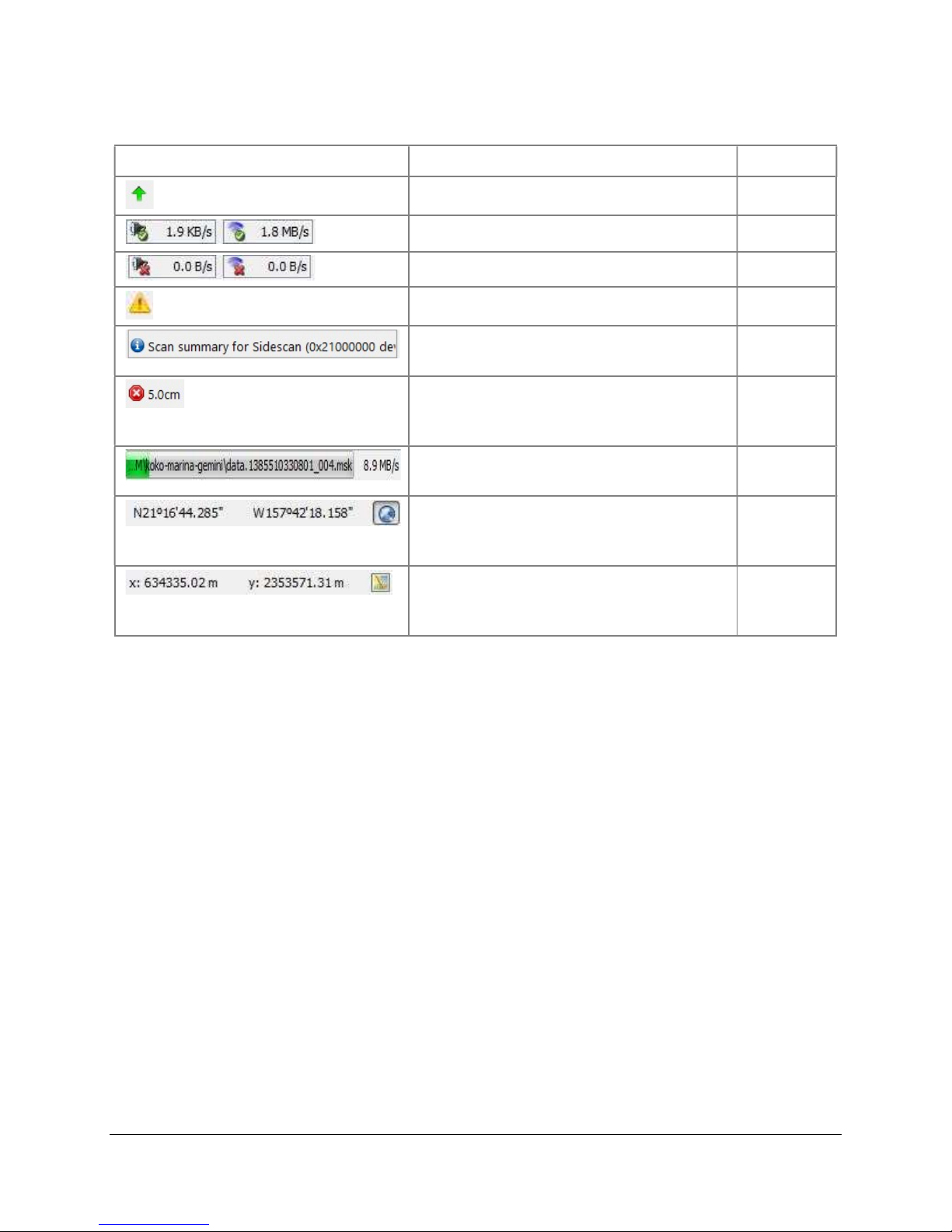
SAMM User Manual
Table
5
. Status bar
Icon/Output Definition Mode
New version available All
Sensors connected, shows data rate Acquisition
Sensors not connected
An error occurred All
Scrolling Event Log bar, click to open the
Event Log window.
Button to cancel file
acquisition/playback/loading, also
indicates current mosaic resolution
File acquisition/playback/loading
progress
Position of cursor in mosaic window in
GPS coordinates, click toggle button for
XY
Position of cursor in mosaic window in
UTM coordinates, click toggle button for
Degrees
Acquisition
All
All
All
All
All
This page is intentionally left blank.
21
Page 24
SAMM User Manual
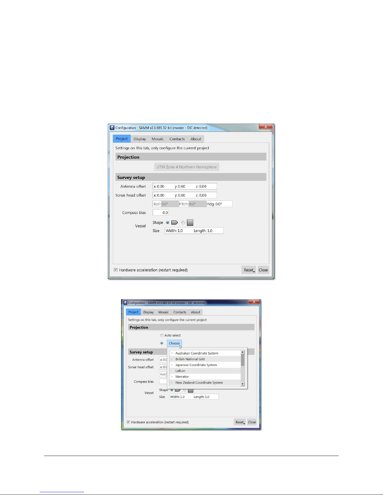
4 Configure SAMM
Before loading or acquiring data in a SAMM project, the user should set up the project in the
Configuration dialog, accessed from the Configuration icon on the main toolbar (Figure 13).
The user has the option to specify survey projection and offsets, units of measure, mosaic
resolution and logging details, contact messaging and review of dongle and license properties.
All of the options are saved as application settings. This section describes each tab in the
Configuration dialog, and provides a tutorial.
Figure 13. Configuration Dialog
Figure 14. Projection Tab
22
Page 25

SAMM User Manual
4.1 Project Tab
The project tab allows the user to configure projected coordinate system and survey settings of
the current project.
4.1.1 Projected Coordinate System
The projection for the mosaic display and exported mosaic images can be set in the Projection
panel in the Project tab of the Configuration window, before data are added to the project
through acquisition, playback, or file loading (Figure 14).
SAMM expects a navigation positioning message in degrees latitude/longitude in the WGS 1984
datum (i.e. standard NMEA GPS message) By default, (with the “Auto Select” option) SAMM
projects the GPS navigation input to Universal Transverse Mercator (UTM) zones (WGS84
datum), performs calculations in UTM meters, and projects the background charts to the UTM
zone to produce the aligned map.
Note: UTM zones cover six degrees of longitude, run from 80° S to 80° N, are numbered from 1
to 60, and are lettered N or S according to the northern or southern hemisphere. Zone
numbering starts at -180 degrees longitude (Midway Island, and the International Dateline) and
increase to the east. Hawai‘i, for example, is mostly in Zone 4, while the US East Coast is
around Zone 18, and the United Kingdom is Zone 30, at Greenwich. The UTM zones are also
available on the NAD27 and NAD83 datums.
The following projected coordinate systems are also supported in SAMM: Australian Coordinate
System, British National Grid, Japanese Coordinate System, Geodetic (lon/lat WGS 1984),
Mercator (Equator), New Zealand Coordinate System, and the U.S. State Plane Coordinate
System (NAD27 and NAD83). The list also includes User Defined coordinate system. However,
the tool necessary to create user defined coordinate system is not available at the moment.
SAMM will support this in the future. If you would like to use a projection that is not supported,
please contact OIC.
SAMM will project the sonar image and background charts on-the-fly to the coordinate system
set in the Configuration window. You may only set the projection before data are added or
acquisition begins. Please keep this in mind when creating projects. To manually change the
mosaic display projection from the default UTM WGS84:
Click the Configuration icon.
Select the Project tab in the Configuration window.
In the Projection panel, choose the coordinate system by clicking on one in the Choose
dropdown menu.
Click outside of the Choose menu to hide the menu.
Click Close.
As soon as data acquisition begins, the projection and UTM zone are locked for that project. If
you would like to use a different projection or zone, please create a new project.
4.1.2 Sensor Offsets
Unless the sonar is co-located with the navigation source, SAMM must approximate the actual
sensor position in order to produce the sonar image and mosaic. The Survey setup panel in the
Project tab in the Configuration window provides input fields for the vessel dimensions and
23
Page 26
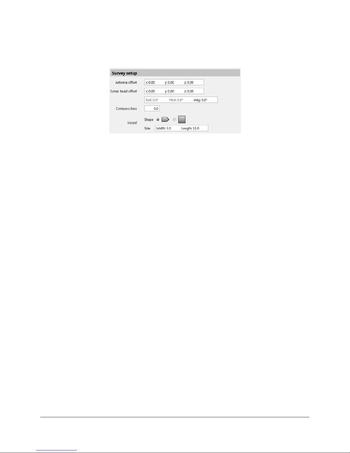
SAMM User Manual
translational and rotational offsets associated with the sonar, navigation, and heading sensors
(Figure 15).
Figure 15. Survey Setup Panel
The fields are defined as follows.
Antenna offset: the distance of the GPS receiver antenna from a reference point in
common with the sonar head offset. The numbering convention is:
X = Port / Starboard (positive number = starboard, negative number = port).
Y = Fore / Aft (positive number = fore, negative number = aft).
Z = Height (positive number = above reference point, negative number = below
reference point).
Sonar head offset: the distance of the sonar head from a reference point in common with
the antenna offset. The same numbering convention is used as for the antenna offset.
Sonar heading offset: the sonar mount bias, i.e., the angular difference between the
centerline of the boat and the actual pointing direction of the sonar.
Pitch and roll offsets: The pitch and roll offsets are not relevant to 2D imaging sonar, and
as such are not yet available.
Compass bias: the heading source mount bias, i.e. the difference between the reported
pointing direction of the heading source and the actual pointing direction of the heading
source. If you have a magnetic compass and know the declination (the difference
between north and magnetic north) for the survey, add it to this bias field. (Automatic
magnetic declination based on lon/lat is not available at this time.)
Vessel: the shape, width, and length of your vessel. These fields define how the vessel
outline is drawn in the mosaic window.
SAMM draws the vessel, GPS antenna and sonar head in the mosaic window in reference to
the center of the boat. Please note that the antenna and sonar head crosshairs will be
incorrectly placed in relation to the vessel outline if you choose to use the location of either the
GPS unit or the sonar head as the reference point. The mosaic is otherwise unaffected. The unit
of measure for the x, y, and z offsets must match the unit for distance and vertical distance in
the Display subpanel of the Configuration window (see Section 4.2.3).
4.2 Display Tab
Display tab contains General, Swath colormap, and Units of measure panels.
4.2.1 General
The General panel in the Display tab in the Configuration window allows the user to change UI
appearance between normal and dark UI mode (Figure 16).
24
Page 27

SAMM User Manual
Figure 16. General Panel
To change the UI appearance:
1. Click the Configuration icon.
2. In the General panel in the Display tab, check/uncheck the Dark UI box.
3. Click Close.
4.2.2 Swath Colormap
The Swath colormap panel in the Display tab in the Configuration window enables the user to
change the swath display colors of default and mosaic in progress (Figure 17). During
processing, SAMM displays imagery data in the mosaic window and PPI by matching pixel
values to screen colors using the colormap. Changing the colormap may highlight different
objects in the subsea environment.
Figure 17. Swath Colormap Panel
The “Mosaic in progress” swath refers to the swath that SAMM is currently mosaicking.
The ”Completed” swaths are those swaths that are completely mosaicked. SAMM has nine
built-in colormaps: goldenrod, copper, reverse gray, grayscale, bone, cool, green, hot, and jet
(rainbow). Each colormap brings out different features of the data.
To change the colormap for swaths:
4. Click the Configuration icon.
5. In the Swath colormap panel in the Display tab, click the dropdown menu for the swath
type and click the desired colormap.
6. Click Close.
4.2.3 Units of measure
Display units may be changed from the Units of measure panel in the Display tab in the
Configuration window (Figure 18).
Table shows the parameter, available units, and affected display area.
Figure 18. Units of Measure Panel
25
Page 28

SAMM User Manual
Value
Units
Affected Display Area
Easting/Northing
Longitude/Latitude
Distance
Vertical Distance
Speed over
Speed of sound
Temperature
Table 6. Parameters and Units
Meters
Feet
Yards
Degree minute seconds
Degree decimal minutes
Decimal degrees
Meters
Feet
Yards
Meters
(depth/altitude)
ground
To change the units of measure:
1. Click the Configuration icon.
2. In the Units of measure subpanel in the Display tab, click the dropdown menu for any
field and click the desired unit.
3. Click Close.
Feet
Yards
Fathoms
Meters per second
Feet per second
Knots
Meters per second
Feet per second
Degrees Celsius
Degrees Fahrenheit
Degrees Kelvin
Status bar
Live Info
Status bar
Contacts
Contacts
Measure Tool (not yet available)
Survey Setup subpanel of Configuration
window
Live Info
Contacts
(Not yet implemented)
Live info
Properties
4.3 Mosaic Tab
Mosaic tab provides options how SAMM creates mosaic and data files.
4.3.1 General
General panel allows the user to change the default resolution of the mosaic and how SAMM
starts a new swath (Figure 19). This sets the highest resolution of the mosaic, but does not
change the logged data. In this section you can also direct SAMM to generate a new swath
automatically if time gap between successive pings is greater than the user specified limit. This
can be useful for automatically creating new swaths in file playback or loading.
Figure 19. General Panel
26
Page 29
SAMM User Manual
4.3.2 MSK output (connected/live sonars)
SAMM provides three methods for creating a new file during data acquisition: manually, break
by duration, and break by file size (Figure 20).
Figure 20. MSK output Panel
SAMM's default file break method is to break by file size when the size reaches 120 MB.
To change the file break method:
1. Click the Configuration icon.
2. In the MSK output panel in the Mosaic tab, click the radio button corresponding to the
desired method.
3. Click Close.
When breaking manually, the user simply select the “New Swath” icon on the toolbar, or
presses the “B” key on the keyboard. Raw data rates from modern sensors can easily exceed
100KB/sec. While workstations, media, and operating systems can handle large file sizes,
please consider your workflow, memory, and file transfer limitations before deciding to break
files manually. Please also consider that data loss due to corruption is significantly more
catastrophic for single large files than single small files.
SAMM automatically names files by combining the time the file was created with an incremental
number.
4.4 Contacts tab
SAMM can send contacts over the network or a serial connection. Each contact is sent as a
proprietary NMEA sentence ($POIT) (Figure 21).
Figure 21. Contacts Tab
To send contacts:
1. Click the Configuration icon.
2. In the Contacts tab, click Not configured to configure the connections.
3. Open the Contact Viewer.
27
Page 30

SAMM User Manual
4. Select contacts.
5. Right click and select Add contact(s) to staging table.
6. In the staged toolbar, click on the Send contact(s) button.
4.5 About
The about tab provides dongle license information, SAMM version information and OpenGL
information (Figure 22).
Figure 22. About Panel
If your license supports it, and if a newer version is available, it can be automatically
downloaded from OIC’s internet server by clicking the Check for updates button (Figure 23).
Figure 23. Update Panel
4.6 Rendering Method
SAMM either uses software or hardware to render swaths and perform computations. The
method used depends on your available hardware, which SAMM auto detects. SAMM uses
hardware rendering if you have a GPU, either integrated in the CPU or video card. SAMM's
mosaic window and PPI have higher quality images when using a GPU to render the sonar
data. If you do not have a GPU, SAMM uses software rendering. If SAMM detects multiple
crashes, it will automatically ask if you want to switch to software rendering upon launch (Figure
24). You can select this via the check-box option at the bottom of the configuration dialog
Figure 24. Crash Detection Prompt
28
Page 31

SAMM User Manual
Configuration
Yes
Configuration
Table describes the two ways to change between software and hardware rendering, if you
desire to override SAMM's detected method.
Table 7. Change the Rendering Method
After launching SAMM: Upon the launch prompt:
1. Click the
icon in the main toolbar.
2. Check/uncheck the
Hardware Acceleration
box.
3. Click Close.
4. Click the Close icon to
close the project.
5. Click the Close button on
the project selector screen
to close SAMM.
6. Relaunch SAMM.
7. Reopen the project.
4.7 Reset Button
1. Click
to software rendering or
keep hardware rendering,
respectively.
or No to switch
The reset button enables you to reset the window locations and the language prompt. SAMM
remembers the last location of its windows between sessions. Click Window position and
sizes from the Reset button dropdown menu to reset the windows. After clicking the button, you
must close the project and then exit SAMM. Launch SAMM, and then the windows will be
restored to their default location. The Forward Look window opens in front of the mosaic
window. Clicking the Selected language (prompt at next launch) command will display the
language selection dropdown menu upon the next launch.
4.8 Configuration Tutorial
Table provides instructions for configuring a project using the demo data and for data
acquisition.
Table 8. Configure Project
To configure for playback mode with demo
data:
1. Click the
2. Click the Project tab.
3. In the Projection panel, leave the UTM
zone set to Auto select.
4. In the Survey setup panel:
in the Antenna offset field, enter
x:0.00 y: 0.00 z:0.00;
in the Sonar head offset field,
enter x: 1.97 y:-3.35 z: -1.00;
leave the Hdg field set at 0.0;
leave the Compass bias field set
at 0.0;
do not change the boat shape; and
icon.
To configure for data acquisition:
1. Measure your sensor offsets and look up the
declination for your survey, if desired.
2. Click the Configuration icon.
3. Click the Project tab.
4. In the Projection panel, choose the desired
projection for the mosaic display window.
5. In the Survey setup panel:
in the Antenna offset field, enter the
distance of the antenna from the reference
point in the unit set in the configuration
window;
in the Sonar head offset field, enter the
distance of the sonar head from the same
29
Page 32

SAMM User Manual
To configure for playback mode with demo
data:
in the Size field, enter Width: 3.0
and Length: 8.0.
5. Click the Display tab.
6. In the Swath colormap panel,
leave the Mosaic in progress field
set to Goldenrod; and
leave the Completed field set to
Goldenrod..
7. In the Units of measure panel, visually
confirm the Distance and Vertical
distance (depth/altitude) fields are
set to Meters (m). Click the Mosaic
tab.
8. In the General panel, set the Default
resolution to 5.0 cm.
9. The MSK output panel is not applicable
in playback mode. Do not change the
setting.
10. Check that your Configuration window
matches Figure 25.
To configure for data acquisition:
reference point using the same numbering
convention;
in the Hdg field, enter the heading bias in
degrees;
in the Compass bias field, enter the
heading mount bias plus the declination of
your survey location in degrees;
choose your vessel shape; and
in the Size field, enter the length and width
of the boat in the unit set in the
configuration window.
6. Click the Display tab.
7. In the Swath colormap panel, choose the
desired colormap for active, inactive, and
selected swaths.
8. In the Units of measure panel, set the distance
and vertical distance units to the unit of your
measured antenna and sonar offsets. Click
the Mosaic tab.
9. In the MSK output panel, choose the desired
method by which to break raw data files.
Figure 25. Configuration Window for Demo Data
30
Page 33

SAMM User Manual
5 Charts and Background Images
SAMM's robust chart module enables you to load a wide variety of charts and geospatial data
files as background layers in the mosaic window. The Chart Display Options window interfaces
to the chart module, which is integrated with Global Mapper™ software.
This section describes the basic and advanced interface in the charts module, the differences
between raster and vector data formats, how to retrieve National Oceanic and Atmospheric
Administration (NOAA) Electronic Navigational Charts® (ENCs) the elements of the basic Chart
Display Options window and the elements of the advanced Chart Display Options window. It
concludes with a tutorial on how to load charts to the advanced interface and a table of
commands for customizing the chart display.
5.1 Basic vs. Advanced Interface
The Chart Display Options dialog has a standard and advanced interface. In the basic interface,
charts are added by file to the project. This manual loading method is also available in the
advanced interface. The chart module saves manually loaded files to the project, not to the
application. In the advanced interface, users have the additional capability to add charts by
folder to the charts database, which are saved to the application. Files added by folder are then
available in any SAMM project. Both interfaces have the option of displaying the ArcGIS Web
Mapping Service World Imagery basemap underneath locally added files. An Internet
connection must be available for this option.
5.2 Raster vs. Vector File Types
Geospatial data are stored as two types: raster orand vector. Vector files have data stored in the
files as features, i.e. as points, lines, polygons, and/or text. These features resize in SAMM
when the mosaic window resolution is changed. Some common vector file types include NOAA
ENCs (S-57 format), National Geospatial-Intelligence Agency Digital Nautical Charts® (VPF
format), and ESRI shapefiles. Raster files, including NOAA Raster Navigational Charts® (BSB
format) and GeoTIFFs, are image files with data stored as a grid of pixels. The text and other
features are static, and grow with the zoom level.
While Global Mapper supports rendering many different types of files, SAMM has only been
thoroughly tested with standard navigational chart types, shapefiles, and GeoTIFFs.
5.3 Retrieve NOAA Electronic Navigational Charts
If you do not have any nautical charts, follow these brief instructions to retrieve NOAA ENCs for
your state. Web sites do change, so we cannot guarantee that these instructions are current.
Skip to section 5.4 if you already have charts.
1. Go to the NOAA Office of Coast Survey Chart Downloader Web site
(http://www.charts.noaa.gov/?Disclaimer=noaa%21nos%40ocs%23mcd&Submit=Proce
ed+to+Chart+Downloader).
2. Next to the second picture, click on the ENCs link.
3. Click on your state in the ENCs by State table.
4. Read the User’s Agreement. Click OK.
The charts automatically download to your browser’s default download folder.
31
Page 34

SAMM User Manual
5. Open the folder containing the charts.
6. Right-click on the charts folder ([State initials]_ENCs.zip) and select Extract All.
7. Click Browse.
8. Navigate to a local disk or network drive to save the folder. Be sure to note the location
where you save the file so that you can find it in the next step. (This is the location of
your chart database that you will point to in SAMM in the next section.)
9. Click OK.
10. Click Extract.
NOAA updates charts nationwide weekly via a notice to mariners. If you are using your charts
for navigational purposes, make sure to get new charts or check for updates.
5.4 Elements of the Basic Chart Display Options Window
The basic chart display options window, launched by clicking the Chart background options
icon in the toolbar, hosts the chart database list and several buttons. Figure 26 shows an empty
chart database list in the basic window. The basic chart loader saves information on a perproject basis.
Figure 26. Empty Basic Chart Display Options Window
The basic chart display options window has a Load chart... button to load charts to the mosaic
window, and provides the option to add the ArcGIS World Imagery basemap with an on/off
checkbox. The Advanced button changes the chart display to the advanced interface, the Set
as default button saves the current settings as the automatic chart display options to the
application, and the Close button closes the Chart Display Options window. The next time the
window is called, it will open to the last interface viewed.
To load charts or other geospatial data files to the chart database list:
1. Click the Load chart... button.
32
Page 35

SAMM User Manual
2. In the Manual Load Chart window, navigate to the file location of your saved charts
(C:\SAMM_DEMO\demo_data\charts).
3. Click on a file to select it (you may select multiple files).
4. Click Open.
5.4.1 Basic Chart Display Popup Windows
The Manual Load Chart window enables you to select any file type present in the folder you are
viewing. This is because Global Mapper supports many different file formats. Geospatial data
are often stored in more than one file. If you select a support file, not the file that SAMM
renders, you will be prompted to select the file format, as shown in Figure 27. This window
appears whenever Global Mapper cannot tell what file type you have attempted to load.
Figure 27. Select Overlay Type Error Message
If this window appears, you likely picked the wrong file type from a family of files sharing the
same name, but with different file extensions. If you know you picked the correct file, then you
can pick the file type from the list and click OK. If you are not sure,
1. Click Cancel.
2. In the chart database list, right-click on the orange Loading... file and click Unload.
3. Click the Load chart... button again.
4. Select all files of the same name in the family and click Open. SAMM will load the
correct one, and try to load the incorrect ones.
5. You may get the Select Overlay Type window again for the support files. Click Cancel.
6. Give SAMM a moment to load the correct file (watch for one to turn green. The
description will match the correct file).
7. Select all of the orange Loading...files (these will be the incorrect files from the family),
right-click and click Unload.
33
Page 36

SAMM User Manual
If you choose to load a text file, you will be presented with the Generic ASCII Text File Import
Options window (Figure 28).
Figure 28. ASCII Text Import Options
If you accidentally loaded the text file, click Cancel, then unload the orange Loading... file in the
chart database. If you intentionally loaded the text file, specify the format of the text file using
the fields in the window. SAMM will render two-dimensional point or point, line, and area files.
5.4.2 Using the Basic Chart Loader
Figure 29 shows the sample charts (ENC, RNC, air photo) loaded in the charts database.
Figure 29. Charts Loaded in Basic Window, with Context Menu
34
Page 37

SAMM User Manual
The pin and green color coding are automatically displayed in the database table on any chart
added manually, whether in the basic or advanced interface. The pin means that the chart
cannot be unloaded by SAMM's auto load function, a feature of the advanced interface. Green
highlighting means that the chart is loaded in the mosaic display, whether through manual or
automatic loading.
You can control which charts display in the mosaic window from the context menu, accessed by
right-clicking on a file. The available commands follow.
Unpin loaded charts: Allows the auto load function to recognize the chart.
Disable charts: Prohibits rendering the chart, even if it is loaded.
Unload: Removes the chart from the loaded list (and the basic interface).
Hide: Hides the chart from the auto load function, but does not remove it from the
database.
The ArcGIS World Imagery provides high-resolution worldwide coverage. It displays under the
other layers. This service requires an Internet connection.
To turn off the Web service, uncheck the box.
5.5 Elements of the Advanced Chart Display Options Window
The advanced Chart Display Options window is accessed by clicking the Advanced button in
the basic Chart Display Options window. From the advanced window, you can populate the
database by scanning folders for supported files; preview the files; and customize your chart
display by configuring the auto load function, manually adding files, pinning files in the
database, and turning the world imagery on and off. The folders added in the advanced
interface are preserved between SAMM projects, so a chart database can be built during first
time use and will be available in all SAMM projects.
35
Page 38

SAMM User Manual
Tabs
Chart Data
base
Table
Buttons
Figure 30. Chart Display Options Window upon Launch
The advanced window includes four tabs: Charts, Folders, Chart Preview, and Log. The chart
database table, tab toggles, and buttons appear on every tab (Figure 30). The database table,
appearing as the top panel, lists the geospatial data files that are present in the chart database
as well as manually loaded charts. They are highlighted in every tab according to the legend
appearing on the Charts tab. Unlike the basic window, the advanced table includes columns for
the description, type, scale or area, and file path of each file. Files added by folder in the
advanced window do not appear in the basic interface.
From the table, you can sort the table by column and select, unpin, disable, unload, and hide
charts. The context menu features are the same as those available in the basic interface, except
that when charts are unloaded, they do not disappear from the list.
To sort by column, click on the column name.
To resize the columns, click and drag on the border.
To access the context menu, right-click on a chart.
5.5.1 Buttons
The Show options button shows or hides the advanced interface tab content.
The Manual load... button opens the manual load window.
The Basic button toggles back to the basic chart display options interface.
The Set as default button saves the current chart auto loading options and world
imagery status as the default settings in the application.
The Close button closes the Chart Display Options window. The next time the window is
called, it will open to the last interface viewed.
36
Page 39

SAMM User Manual
5.5.2 The Folders Tab
The Folders tab enables you to populate the chart database from folders stored on your local
hard drive or network. Figure 31 shows the add/scan charts panel of the Folders tab.
Figure 31. Add/Scan Charts Panel
The Add folder... allows users to browse to folders containing chart files and add them
to the list of folders to be searched for charts.
The Remove folder button removes files/folders from the add/scan charts panel. All
charts located within the folder are removed from the database as well.
The Scan for new charts button scans files from the listed folders and adds them to the
database (and populates the database table). Press this after you add a folder.
Populating the Charts Database
Adding a chart to the database makes it available for use in future projects without having to
manually add it. To do this:
1. Add folders: On the Folders tab, click the Add folder... button and navigate to the
location holding the folder. Click on the folder to select it and click Select Folder. Add as
many folders as you have containing relevant geospatial data. The scanning algorithm in
the next step will recursively search inside all subfolders. For simplicity, consider saving
all of your background layers in one main folder and add that folder to SAMM. Take care
to preserve the file structure of any acquired DNC folders, or the scanning algorithm may
not recognize the charts. When the scanner finds a folder containing a file named LHT, it
stops looking for compatible data because the LHT file means that it has found a DNC.
Data that are not DNC data stored inside a folder with a DNC LHT file will be lost.
2. Scan folders: After you have added your main charts folders and your root DNC folders,
select a folder in the list and click Scan for new charts. This process runs in the
background so you may continue working in SAMM, with the exception that adding
another folder will stop the scanner (rescan the folder if this happens). The scanning
function finds all files in the selected folder that are compatible for display in SAMM.
Once SAMM has scanned the folders, the available files appear in the database table (Figure
32). The auto load function in the advanced interface selects charts from this database to
display.
37
Page 40

SAMM User Manual
Figure 32. Populated Chart Database
5.5.3 The Chart Preview Tab
The previewing charts tab of the advanced interface enables viewing any chart in the database.
This helps you get a feel for each type of chart file, if you are unfamiliar, and also shows you the
geographic extent and level of detail present in each file. To preview a chart, click on the chart
preview tab. The chart highlighted in the database shows in the viewing window. Click on a
chart to highlight it. Resize the chart preview panel with a click and drag on the panel border.
38
Page 41

SAMM User Manual
5.5.4 The Charts Tab
The Charts tab is the default tab displayed (Figure 33).
Figure 33. Charts Tab
By default, the Auto load and Online world imagery checkboxes are checked. Uncheck them
to disable the features. The auto load feature loads the files from the chart database that most
closely match the resolution (raster) or coverage (vector) of the mosaic window extent into the
mosaic window. It constantly looks for charts that satisfy its criteria, set in the Load by
raster/vector and Load by chart type fields.
The load by raster/vector feature loads charts up to the number entered per type of data
file (raster or vector). Click in the Raster or Vector fields and enter a number to change
the numbers.
The load by chart type feature loads charts of the specific format up to the number per
format (VPF for DNC, S-57 for ENC, BSB for RNC, GeoTIFF, shapefile, etc.). Formats
are listed in the Type column as they are loaded to the chart database. The list doesn't
forget any file types loaded in all of SAMM's history, so it may present file types that are
not present in the database anymore. This happens when you unload the source folder.
Click in the types fields to enter the number per file type that the auto loader should load.
Toggle between the method that the auto load algorithm uses to load charts by clicking on the
buttons. The auto loader indicates which method is in use by highlighting the button in blue.
The display options and legend refer to the database table.
The Show hidden charts box unhides files hidden from the table. It does not unhide
them from the auto load algorithm. To do this, you must right-click on the chart and click
Unhide.
5.5.4.1 Color Coding
SAMM color codes the charts in the database so that you can see what charts will be rendered
and what charts might be available for rendering. The legend is shown on the Charts tab, but
the color coding is used on all tabs of the advanced interface. Only the green, loaded charts
display in the basic interface.
39
Page 42

SAMM User Manual
Green
Charts that are loaded are bright green and will be rendered, unless they are disabled. (You
may want to disable a chart, instead of unloading it, to prevent the autoloader from replacing it
in the display.) Green charts were either automatically loaded because they meet the auto
loader's criteria, or they were manually loaded through either
a. the Manual load... button, or
b. the Load command available on the right-click menu on a chart in the database.
Unless the database has been sorted, the green loaded charts always appear at the top of the
list, in the order of smallest vector first, then higher resolution rasters.
Orange
Orange highlighting is transient. These charts are loading, so the orange indicates that SAMM is
actively loading them to the mosaic window. They will turn green when they are loaded.
Yellow
The yellow charts follow; these are yellow because they
a. don't meet the auto-load criteria but intercept the mosaic window extent or
b. they were manually unloaded using the Unload command from the database context
menu.
The yellow charts are within the vicinity of the project, and are available to the autoloader if the
auto load settings are changed. The charts are ordered using the same convention as the green
ones, with vectors covering the smallest area first, then rasters of higher resolution. If the
database is sorted, they will reorder according to the sort but this does not affect the display.
Gray
Hidden charts are highlighted in grey, when they are shown. They are hidden from the auto
loader. You may toggle their display in the chart database on and off from the Show hidden
charts checkbox under Display options on the Charts tab.
Manually Loaded vs. Folder Added Chart Behavior
SAMM's chart loader determines how to treat a chart based on how it was loaded. You can
force the manually loaded or folder added behavior using the context menu commands.
SAMM's auto load algorithm either recognizes a chart in the database as suitable for loading, or
it doesn't. If it doesn't recognize the chart, that chart file has either been pinned, so it can be
rendered, or it is hidden, and it cannot be rendered. SAMM automatically pins every chart that
has been loaded manually, either in the basic interface or using the Manual load... button in the
advanced interface. You can also pin any chart by right-clicking on it in the database list and
clicking Pin Loaded Chart (if the chart is already loaded) or clicking Load (to load the chart,
which SAMM then automatically pins), or double-clicking on the chart.
You can hide any chart from the auto load algorithm by right-clicking on it and clicking Hide. It
disappears from the database list, but will display if you click the Show hidden charts box on
the Charts tab. To reveal these charts to the auto load algorithm, you must right-click on the
hidden chart and click Unhide. If you click Load on a hidden chart, it will load it and then pin it.
It will still be hidden from the algorithm, but will then be available for rendering.
40
Page 43

SAMM User Manual
Chart
Chart
Chart
Advanced
Advanced
Advanced
Command
Action
Charts added through a folder (and therefore added to the charts database) will not be available
in the basic interface, unless you manually pin them or the autoloader has loaded them. The
autoloader looks at these charts in order to find charts suitable for rendering.
Every loaded chart has the option to be disabled, or to prevent it from rendering without hiding
it. This keeps the chart in the loaded station, which means the autoloader counts it as a loaded
chart, but the chart does not render.
5.5.5 The Log Tab
The log tab reports errors in the chart module, including the database, scanner, and renderer.
5.6 Advanced Chart Loader Tutorial
There are three ways to display background content in the mosaic window using the advanced
interface. To load background layers in SAMM, follow the steps in Table .
Table 9. Load and Display Charts
To auto load files from folders: To load Web-hosted content: To load individual files:
1. Click the
background options icon
in SAMM’s toolbar.
2. Click the
button.
3. Click the Folders tab.
4. Click Add Folder.
5. Navigate to and click the
folder containing charts
and/or
geocoded files.
6. Click Select Folder.
7. Click Scan for new
charts.
8. Click the Charts tab.
9. Ensure the Auto load box
is checked.
10. Click Close to exit the
window.
1. Click the
background options icon
in SAMM’s toolbar.
2. Click the
button.
3. Stay on the Charts tab.
4. Ensure the Online chart
box is checked.
5. Click on the type of map or
imagery you want to select
it.
6. Uncheck the Auto load
box (for the playback
tutorial).
7. Click Close to exit the
window.
1. Click the
background options icon
in SAMM’s toolbar.
2. Click the
button.
3. Stay on the Charts tab.
4. Click the Manual load...
button on the bottom of
the window, next to the
Close button.
5. Navigate to and click the
chart (or other geocoded
files).
6. Click Open.
7. Click Close to exit the
window.
5.7 Chart Customization Commands
The features for customizing the chart display are collected in Table with the methods available
to execute the commands.
Table 10. Chart Customization Commands
Select chart
Select multiple adjacent
charts
In the chart database table, click or right-click on the chart.
In the chart database table, click on the first chart, hold Shift,
and click on the last chart.
41
Page 44

SAMM User Manual
Command
Action
Select multiple non-adjacent
charts
Hide charts from chart
database table
Show hidden charts in chart
database table
Unhide hidden charts
Turn hide/unhide a chart from
the auto loader while keeping
the chart loaded
Unload manually loaded chart
from the chart database table
Enable/Disable forced display
of a loaded chart in the
mosaic window
Restrict the auto load feature
to a certain number of
raster/vector charts
Restrict the auto load feature
to a certain number of charts
by chart type
Turn the world imagery on/off
Disable the auto load function
In the chart database table, click on the first chart, hold Ctrl,
and click on each subsequent chart.
In the chart database table, right-click on the chart and click
Hide.
In the display options and legend panel of the Charts tab,
click the Show hidden charts checkbox.
After showing the hidden chart, in the chart database table,
right-click on the charts and click Unhide.
In the chart database table, right-click on the chart and click
Pin loaded chart/Unpin loaded chart.
In the chart database table, right-click on the chart and click
Unload.
In the chart database table, check/uncheck the box next to
the chart.
In the chart database table, right-click on the chart and click
on Disable charts or Enable charts.
In the auto load panel of the Charts tab, ensure the Auto
load box is checked, then enter the number of raster charts
in the Raster field and the number of vector charts in the
Vector field.
In the auto load panel of the Charts tab, ensure the Auto
load box is checked, then click the Load by chart type
button and enter the number of each type of chart in the
chart type fields.
In the online chart panel of the Charts tab, ensure the Online
chart box is checked and click on the desired service
(imagery, topography, weather).
In the auto load panel of the Charts tab, click the box next to
the Auto load field to uncheck it.
Set the current settings as
default
Preview the chart
In the display options and legend panel of the Charts tab,
click the Set as default button.
In the chart database table of the Chart preview tab, click on
the chart.
42
Page 45

SAMM User Manual
6 Add Files or Begin Acquisition
SAMM can mosaic data in acquisition, playback, or post-processing modes. To mosaic data
properly, SAMM accesses two classes of data: the sonar data itself and metadata. When in
playback or post-processing mode, SAMM gets these data from the raw data files. During
acquisition, however, SAMM receives these data either as they are broadcast from the sonar
software, or directly from the sensors. At this time, Marine Electronics, R2Sonic, Tritech Gemini
and Imagenex 881L-GS/882L owners must interface directly with the navigation/heading
sources and the sonar, and other sonar systems interface to the position and heading feeds
with the native sonar software.
The first part of this section describes how to start a project in post-processing or playback
mode by adding data files to the project. The second part describes how to load data from
directory, which can be used to build a near-realtime mosaic during data acquisition. The third
part describes how to interface with the metadata sources, and the Fourth part provides
instructions for interfacing with supported sonar systems. The Add data dropdown menu (Figure
34), accessed by clicking the Add data icon, controls file loading and interfacing with a sensor
or sonar software program.
Figure 34. Add Data Dropdown Menu
6.1 Add Files in Playback or Post-Processing Mode
Supported data formats for post-processing and playback include M3 processed data files
(*.imb), BlueView (*.son), ARIS/DIDSON (*.aris/*.ddf), Tritech Starfish (*.logdoc), EdgeTech
(*.jsf), Klein (*.sdf), Reson/Norbit (*.s7k) and OIC SAMM (*.msk) and GeoDAS (*.oic). We
suggest you practice with SAMM in playback mode prior to conducting a survey in acquisition
mode.
6.1.1 Load Files
Load files option allows the user to select a collection of data files of the same type to generate
mosaic without viewing the data. The resulting mosaic can be composed of numerous swaths,
each of which is created from raw data files that are continuous in time. Therefore, if the data
files were continuously recorded throughout the survey, the mosaic will have only one swath. If
the data logging was paused during turns, the mosaic will have the number of swaths equal to
the number of survey lines.
To load data files for analysis mode:
43
Page 46

SAMM User Manual
1. Click the Add data icon.
2. Click Load files.
3. Navigate to the directory containing the files.
4. Select files you wish to load. Note that at any one time you can only load the data of the
same format. If you wish to load multiple passes from different sensors, you may do this
only in multiple, sequential loadings (As an example, first create the project and load
forward-look data and create swaths. Then when those files have finished mosaicking,
you can load sidescan data from the same are, and SAMM will create new swaths for
them in the same project.)
5. Click Open.
6. Monitor file loading progress in the status bar on the bottom right. The swaths display
when all files are loaded.
6.1.2 Advanced Load Files
Advanced load files option enables the user to select data files of the same type from multiple
locations as well as to specify mosaicking options (Figure 35).
To load data files in Advanced load files mode:
1. Click the Add data icon
2. Click Advanced load files icon.
3. Navigate to the directory containing the files.
4. Select files you wish to load. Note that you can only load the data of the same format.
5. In the Advanced Load dialog, add more files or remove selected files as necessary.
6. Set mosaic resolution.
Figure 35. Advanced Load Dialog
44
Page 47

SAMM User Manual
7. Set mosaicking options or FLS or SLS data. For FLS data, set the arc and range, as well
as ground range(altitude data needs to be recorded) and invert beams. For SLS data,
set the minimum and maximum clipping ranges, ground range option and layback
options.
8. Set the gamma, brightness, horizontal feathering and vertical feathering of swaths.
9. Click Advanced Load.
10. Monitor file loading progress in the status bar on the bottom right. The swaths display as
each file is loaded.
6.1.3 Playback Files
Playback files option allows the user to replay the survey and watch mosaic being created with
user inputs such as breaking the swath at line turns and marking targets.
To Add data for playback mode:
1. Click the Add data icon.
2. Click Playback files.
3. Navigate to the directory containing the files (C:\SAMM_DEMO\demo_data).
4. Click on a file, then press Ctrl+A to select all of them. Note that you can only playback
data of the same format.
5. Click Open.
6. Monitor file loading progress in the status bar on the bottom right.
7. Click the Start button on the playback controls. The survey playback begins and mosaic
starts to build up.
6.1.4 Advanced Playback Files
Advanced playback files option allows the user to playback data files of the same type that are
stored in multiple locations as well as to specify mosaicking options (Figure 36).
45
Page 48

SAMM User Manual
Figure 36. Advanced Playback Dialog
To load data files in Advanced load files mode:
1. Click the Add data icon.
2. Click the Advanced playback files icon.
3. Navigate to the directory containing the files.
4. Select files you wish to playback. Note that you can only playback the data of the same
format.
5. In the Advanced Playback dialog, add more files or remove selected files as necessary.
6. Set mosaic resolution.
7. Set mosaicking options or FLS or SLS data. For FLS data, set the arc and range, as well
as ground range(altitude data needs to be recorded) and invert beams. For SLS data,
set the minimum and maximum clipping ranges, ground range option and layback
options.
8. Set the gamma, brightness, horizontal feathering and vertical feathering of swaths.
9. Click Advanced Playback.
10. Monitor file loading progress in the status bar on the bottom right.
11. Click the Start button on the playback controls. The survey playback begins and mosaic
starts to build up.
46
Page 49

SAMM User Manual
Figure 37 shows SAMM’s GUI playing the sample data.
Live info, playback controls and processing controls appear in the Swath list’s place, and
the list has shifted to below the processing controls.
data.1385510330801_037_ds.msk, referenced in the Swath list, is drawn behind the
vessel in the mosaic window.
World imagery is layered under the vessel and swaths in the mosaic window.
The Add data icon has a small red x; press this to stop adding data.
The file playback progress is present in the status bar.
Figure 37. GUI in Playback Mode
This is the standard SAMM playback mode. You can pause, restart, slow down or accelerate
playback. During playback you can break swaths (use the Break swath button or B key), adjust
swath properties and update charts/views.
SAMM does not support adding data from widely disparate locations to the same project at this
time. Please start a new project for each new region of operation.
6.2 Load Files from Directory
Similar to the Load files function, SAMM can load files from a selected directory. This mode
allows SAMM to monitor the selected directory and when new files are added to the directory,
SAMM automatically grabs them and adds to the mosaic. This mode is useful for sonar systems
to which SAMM currently does not interface in real-time but supports playback/load of the data
formats (e.g. Sound Metrics ARIS/DIDSON, Reson FLS, MST and XTF sidescan). During a
survey, as data acquisition software writes a new file to a folder that SAMM is monitoring, the
file gets loaded to SAMM and the mosaic updates. The update rate of the mosaic depends on
how often the data acquisition software writes data to a file. If a file creation interval is set small
(e.g. 10 seconds), SAMM can create mosaic in near-realtime.
47
Page 50

SAMM User Manual
Load from directory window allows the user to set up how the data files are loaded (Figure 38).
Figure 38. Load from directory dialog
To load data files from directory:
1. Click the Add data icon.
2. Click Load from directory.
3. Click Browse... and navigate to the directory where you want to load files.
4. For the Action to be taken item, select one of the 3 modes:
Load existing files only
Monitor and load new files, include existing files
Monitor and load new files only
5. Select file type from the dropdown list. Note that SAMM can load data files of the same
type.
6. Set mosaic resolution.
7. Processing options enables the user to set processing parameters for mosaicking (See
Section 7.4 for detail).
8. Click OK.
9. Monitor file queue indicator and file loading progress in the status bar. The swaths
display as files are loaded.
10. To stop file loading when in directory monitor mode, click the Add data icon (with red x).
48
Page 51

SAMM User Manual
NMEA
GreenSea Navigation
6.3 Interface with Metadata Sensors
SAMM can receive the metadata inputs of position, heading, and time (if available) through one
serial port for integrated systems, two serial ports, or a networked GreenSea™ navigation
system. SAMM automatically detects the NMEA data protocols and selects the most accurate
type available. The following string types are listed in order of preference:
Lon/Lat
o PTNL, GGK
o GGA
o RMC
o GLL
Heading
o HDT
o (HDG, HDM, DPT, and RMC are not yet supported.)
Time and Date
o ZDA (While not required for mosaicking, it will increase the accuracy of the
mosaic if available.)
Please set your navigation devices to the highest available data protocol in this list. Please note
that at this time SAMM receives data only in the National Marine Electronics Association
(NMEA) formats. If you have alternative data string formatting, please contact OIC.
SAMM assumes the received lon/lat are on the WGS 1984 datum. This is the most frequently
used datum for navigation systems because it is the datum used by the Global Positioning
System (GPS) satellite constellation. Confirm that your navigational system is set to the WGS
1984 datum.
To configure the metadata input:
1. Click the Add Data icon.
2. Click Connect to...
3. Pick your sonar from the list.
(Navigation/heading interfacing is
required for the Tritech Gemini,
R2Sonic Marine Electronics
Dolphin, BluePrint SubSea Oculus
and Imagenex sonar systems at this
time. All other systems receive
navigation and heading data via
their native software)
4. In the Position and heading options, select
dropdown menu (Figure 39). Enabling GreenSea navigation disables the serial ports.
5. Click the separate heading sensor checkbox if you are using separate heading sensor.
6. Click the Not configured button and select Serial Port or Network.
7. If the Serial port is selected, choose the serial port into which the sensor is plugged and
ensure that the Baud, Data bits, Parity, and Stop bits fields match the corresponding
sensor settings.
8. If the Network is selected, configure the network interface, IP address and port.
9. If you are using two different ports for position and heading, repeat steps 6 through 8 to
configure for the heading sensor.
Figure 39. Navigation Interfacing
or
from the
49
Page 52

SAMM User Manual
6.4 Connect To…
This section describes how to connect SAMM with each brand of supported imaging sonar and
scanning sonar. For each sonar system, default acquisition and processing parameters are
provided, the user may set their own. The following settings are common to all:
Resolution: The size of one pixel in centimeter. Note that setting too small a value may
cause long processing times and dropped packets.
Use ground range: Check this to use ground range correction. This option requires
altitude data to be present. If altitude is not found, processing will default to slant range.
Use course for heading: Check this to use course instead of heading. Some sensors
do not provide heading, but derive course from position.
6.4.1 Kongsberg Mesotech M3
SAMM interfaces with the M3 sonar by receiving a data and metadata string from the sonar
software directly. The M3 sonar software is capable of running in several application modes. If
you run the sonar in EIQ -Fine or EIQ- Ultrafine modes without remaining stationary, the
resulting mosaic may be distorted (see the M3 manual for reference).
To interface with the M3 sonar:
1. Launch the M3 sonar software
and connect the sonar as usual.
2. Launch SAMM.
3. Click the Add data icon.
4. Click Connect to...
5. Select Kongsberg M3 from the
supported sensors list and click
Load.
6. In the M3 interface window
(Figure 40), set processing
parameters as necessary.
7. If SAMM and the M3 software are
running on the same computer, do
not change the IP address from
127.0.0.1. If the sonar software
is running on a different computer
and networked to the SAMM
computer, select an appropriate
network from the Network
interface dropdown and enter the
IP address of the computer
running the M3 software in the IP
address field.
8. Do not change the port number from 20001 unless you change it in the M3 sonar
software. Then, enter the matching port number in the Port field.
9. Click the Connect button.
10. Monitor the connection status in the Device status popup and in the status bar on the
bottom left. Acquisition begins automatically. SAMM flashes a warning if it is not
recording. Click the Record toggle icon to switch recording on and off.
Figure 40. M3 Interfacing
50
Page 53

SAMM User Manual
6.4.2 Kongsberg Mesotech MS1000
SAMM interfaces with the MS1000 series sonar by receiving a data and metadata string from
the sonar software directly.
To interface with the MS1000 sonar:
1. Launch the MS1000 sonar
software and connect the sonar
as usual.
2. Launch SAMM.
3. Click the Add data icon.
4. Click Connect to...
5. Select Kongsberg MS1000 from
the supported sensors list and
click Load.
6. In the MS1000 interface window
(Figure 41), set processing
parameters as necessary.
7. If SAMM and the M3 software are
running on the same computer, do
not change the IP address from
127.0.0.1. If the sonar software
is running on a different computer
that is networked to the SAMM
computer, select an appropriate
network from the Network
interface dropdown and enter the
IP address of the computer
running the M3 software in the IP
address field.
8. Do not change the port number from 5000 unless you change it in the MS-1000 sonar
software. Then, enter the matching port number in the Port field.
9. Click the Connect button.
10. Monitor the connection status in the Device status popup and in the status bar on the
bottom left. Acquisition begins automatically. SAMM flashes a warning if it is not
recording. Click the Record toggle icon to switch recording on and off.
Figure 41. MS1000 Interfacing
51
Page 54

SAMM User Manual
6.4.3 Teledyne BlueView 2D Multibeam Imaging Sonar
Similar to M3 interfacing, SAMM interfaces with the BlueView family of 2D imaging sonar
systems by receiving data and metadata strings from the sonar software, ProViewer. ProViewer,
however, must be configured to push data to SAMM. The following instructions and screenshot
were valid with ProViewer 4 at the time of this writing, but may not be up to date. Please consult
the ProViewer manual for the most accurate instructions.
Figure 42. ProViewer NMEA Panel
Figure 43. ProViewer Data Streaming Configuration
To interface with ProViewer:
1. Launch ProViewer version 4.3 or newer and connect to the sonar as usual.
Configure NMEA settings via the NMEA(GPS) tab in the application settings menu
(Figure 42). SAMM requires GGA, HDT, and ZDA inputs to be configured.
Configure ProViewer for streaming data to SAMM by clicking on the Application
settings icon, clicking on the AppEx tab, Click the checkbox next to RTheta Images,
Nav. Data and Pan/Tilt Data (match Figure 43). If you are running SAMM on a different
computer than ProViewer, enter the IP address in the field. Otherwise, enter the local IP
address (192.168.1.3 if using the IP address suggested in the ProViewer manual). Click
Show Advanced Settings if the IP address in unavailable.
2. Turn on the data broadcasting by clicking the AppEx broadcast on icon in ProViewer.
52
Page 55

SAMM User Manual
3. Launch SAMM.
4. Click the Add data icon.
5. Click Connect To...
6. Select BlueView ProViewer from
the supported sensor list and click
Load.
7. In the BlueView interface window
(Figure 44), set processing
parameters as necessary.
8. If SAMM and ProViewer are
running on the same computer, do
not change the IP address from
127.0.0.1. If ProViewer is
running on a different computer
than SAMM, select an appropriate
network from the Network
interface dropdown and enter the
IP address of the computer
running the ProViewer software in
the IP address field.
Do not change the port number
from 1152 unless you changed it
in the sonar software. Then, enter
the matching port number in the
Port field. (The option to log data
in *.son format is not yet
available.)
9. Click the Connect button .
10. Monitor the connection status in the Device status popup and in the status bar on the
bottom left. Acquisition begins automatically. SAMM flashes a warning if it is not
recording. Click the Record toggle icon to switch recording on and off.
Figure 44. BlueView Interfacing
53
Page 56

SAMM User Manual
6.4.4 Tritech Gemini 720i/is, Marine Electronics Dolphin, Blueprint Oculus, or R2Sonic
For the Kongsberg and BlueView sonars, SAMM receives the sonar data and metadata through
the respective software packages. For the Tritech Gemini, Marine Electronics Dolphin, Blueprint
Subsea Oculus and R2Sonic in forward-looking mode, SAMM interfaces directly with the sonar,
so no native sonar software need be run. Please exit and native sonar program before
launching SAMM, and note that you must complete interfacing with the navigation sensors in
SAMM before beginning acquisition of data.
To interface with the Gemini, R2Sonic
Oculus or Dolphin sonars:
1. Connect the sonar as usual.
2. Launch SAMM.
3. Click the Add data icon.
4. Click Connect to...
5. Select Tritech Gemini, R2Sonic,
Oculus or Dolphin from the
supported sensors list and click
Load.
6. In the Connect to Sonar window
(Figure 45), set processing
parameters as necessary.
7. Configure the metadata input for
position and heading (see section
6.3).
8. Click the Connect button.
9. Monitor the connection status in
the Device status popup and in
the status bar on the bottom left.
Acquisition begins automatically.
SAMM flashes a warning if it is
not recording. Click the Record
toggle icon to switch recording on
and off.
Troubleshooting
If you experience connection problems with your sonar, try to solve or isolate the connection
problem using the following steps:
1. Close SAMM and launch the native sonar software. If the sonar software does not work,
consult the sonar’s owner’s manual to solve the connection issue. Please note that the
native sonar software and SAMM cannot run at the same time.
2. If you are still not receiving sonar data in SAMM (but the native sonar software works),
you may try to:
Disable all network adaptors other than the Ethernet port that the sonar is
connected to in the Windows Explorer Network and Sharing Center. In Windows
7, access this center through the Network and Internet page on your computer's
Control Panel. Then, click Change adapter settings in the left panel. Right-click
on the connections that are not connected to the sonar and click Disable.
Figure 45. Gemini Interfacing
54
Page 57

SAMM User Manual
If the problem persists, you may try to disable your firewall or set a firewall
exception for the SAMM software.
3. If you are not receiving position/heading data:
If using a serial port, please make sure your GPS/compass is outputting NMEA
Lon/Lat message and NMEA HDT messages for heading. Make sure that serial
communication settings in SAMM (baud rate, parity, stop bit) match your device(s).
If you are using GreenSea navigation data, make sure to select the GreenSea
navigation from the Position and heading dropdown menu. This disables the serial
port input.
4. If the PPI does not look correct, try viewing the sonar properties by clicking the
Properties icon on the main toolbar and identifying the problem from the attributes.
Gemini Sonar Controls
The Gemini sonar controls include range and gain slider bars, a checkbox for fixing the sound
velocity, and a checkbox for disabling the auto ping mode (Figure 46).
Figure 46. Gemini Sonar Controls
The range slider enables the user to specify the maximum range the sonar will scan (or ping
period). Longer ranges mean longer ping periods, since the ping must travel further. The gain
slider enables the user to control the relative sonar receive gain. Gemini users may experiment
with this setting according to their preference and water and target conditions; OIC has found
the 60-75% range a useful starting point in our test marina. Setting the gain too high introduces
artifacts into the sonar data (Figure 47).
55
Page 58

SAMM User Manual
Figure 47. Black banding artifacts with high gain and the same data with lower gain.
The current sensor sound velocity displays at sensor depth in the sonar controls box (in
meters/second). The sound velocity value can be overridden by checking the checkbox next to
the Fixed Sound Vel. box. This is typically performed when actual sound velocity sensor data
are not available; the Tritech Gemini is equipped with a sound velocity probe, so sensor data
should be used if accurate. Sound velocity generally varies from 1450 m/s for very cold waters
to 1550 m/s for very warm waters. In most circumstances you do not need to change the sound
velocity.
Auto ping mode is the default mode and should be used most of the time. In this mode, the
sonar controls when it pings; it pings again when it has pushed the last processed ping to the
receiving software. If you disable auto ping mode, the sonar will wait to ping until it has received
the command to ping from SAMM. If the ping backlog gets too high, SAMM may discard some
raw ping records in an attempt to keep up. Auto ping mode is sufficient for most computer
systems and should be used unless SAMM is overwhelmed with ping packets. The Auto ping
mode is analogous to the Continuous mode in Tritech's Seanet Pro software, while disabling the
Auto ping mode is analogous to the Triggered mode.
R2Sonic Sonar Controls
The R2Sonic sonar controls include range (RNG), sector width (WIDTH), brightness (BRT),
sector rotation (ROT), gain (GAIN), power (PWR), pulse length (Plen), and transmit on/off (TX)
(Figure 48). Projector type (PROJ), frequency (FREQ), and time synch method (SYNC) can be
accessed by clicking the advanced setting button. These controls work the same way as the
corresponding controls in the R2Sonic native software.
Figure 48. R2Sonic Sonar Controls
56
Page 59

SAMM User Manual
Marine Electronics Dolphin Sea View
The Dolphin Sea View has a magnetic compass built into the sonar head. If you do not have a
dedicated source of heading, check the box for Bearing to utilize the built in compass (Figure
49).
Figure 49. Dolphin Sea View Interfacing
The Dolphin Sea View controls include range, gain, clutter, resolution, sound
velocity(SoundVel), angle, transmit power(TxPower) and pulse length(PulseLen) (Figure 50).
Figure 50. Dolphin Sea View Controls
57
Page 60

SAMM User Manual
Blueprint Subsea Oculus
The Blueprint Oculus features a gain assist mode, where gain is automatically adjusted during
data acquisition. We highly recommend that you do not enable this function. (Figure 51).
Figure 51. Blueprint Oculus Interfacing
The Blueprint Oculus controls include range, gain, gain assist, gamma, and sound velocity
(Figure 52).
Figure 52. Blueprint Oculus Controls
58
Page 61

SAMM User Manual
.
6.4.5 Edgetech Discover, Klein SonarPro and GeoDAS
SAMM supports mosaicking of sidescan data received from Edgetech Discover, Klein SonarPro
and GeoDAS. Similar to the Kongsberg and Blueview sonars, SAMM receives the sonar data
and metadata through the respective native sonar software packages.
Edgetech Discover
SAMM interfaces with Edgetech sonars by receiving a data and metadata string from the
Discover software directly.
To interface with an Edgetech sonar:
1. Launch the Edgetech Discover
software and connect the sonar as
usual.
2. Be sure to configure NMEA inputs,
GGA, HDT and ZDA.
3. Launch SAMM.
4. Click the Add data icon.
5. Click Connect to...
6. Select Edgetech Discover from
the supported sensors list and click
Load.
7. In the Edgetech Discover interface
window (Figure 53), set processing
parameters as necessary.
8. If SAMM and the Discover software
are running on the same computer,
do not change the IP address from
127.0.0.1. If the Discover
software is running on a different
computer than SAMM, select an
appropriate network from the
Network interface dropdown and
enter the IP address of the
computer running the Discover
software in the IP address field.
9. Do not change the port number from 1900 unless you change it in the Discover
software. Then, enter the matching port number in the Port field.
10. Click the Connect button.
11. Monitor the connection status in the Device status popup and in the status bar on the
bottom left. Acquisition begins automatically. SAMM flashes a warning if it is not
recording. Click the Record toggle icon to switch recording on and off.
15.
Figure 53. SAMM interface to Edgetech Discover
59
Page 62

SAMM User Manual
Klein SonarPro
SAMM interfaces with Klein sonars by receiving a data and metadata string from the SonarPro
software directly.
To interface with a Klein sonar:
1. Launch the SonarPro
software and connect the
sonar as usual.
2. Be sure to configure
NMEA inputs, GGA, HDT
and ZDA.
3. Launch SAMM.
4. Click the Add data icon.
5. Click Connect to...
6. Select Klein 3000/3500
from the supported
sensors list and click
Load.
7. In the Klein interface
window (Figure 54), set
processing parameters as
necessary.
8. If SAMM and the SonarPro software are running on the same computer, do not
change the IP address from 127.0.0.1. If the SonarPro software is running
on a different computer than SAMM, select an appropriate network from the
Network interface dropdown and enter the IP address of the computer running
the Discover software in the IP address field.
9. Click the Connect button.
10. Monitor the connection status in the Device status popup and in the status bar
on the bottom left. Acquisition begins automatically. SAMM flashes a warning if
it is not recording. Click the Record toggle icon to switch recording on and off.
Figure 54. SAMM interface to Klein SonarPro
60
Page 63

SAMM User Manual
GeoDAS
1. Launch GeoDAS and connect to your
sonar as usual.
2. Be sure to configure NMEA inputs, GGA,
HDT, and ZDA.
3. Set up UDP Broadcasting (Figure 55).
Check Enable. Set the port to 5000, and
select the appropriate broadcast IP
address. If SAMM and GeoDAS are
running on the same computer, choose
127.0.0.1, if they are on separate
computers, choose to broadcast on the
IP to which both computers are
connected. Click OK.
4. Launch SAMM.
5. Click the Add data icon.
6. Click Connect to...
7. Select GeoDAS from the supported
sensors list and click Load.
8. In the GeoDAS interface window (Figure
56), set processing parameters as
necessary.
Figure 55. GeoDAS UDP Broadcast Settings
9. If SAMM and GeoDAS are running on
the same computer, do not change the
IP address from 127.0.0.1. If GeoDAS is
running on a different computer than
SAMM, select an appropriate network
from the Network interface dropdown
and enter the IP address of the computer
running the Discover software in the IP
address field.
10. Do not change the port number from
5000 unless you change it in GeoDAS.
Then, enter the matching port number in
the Port field.
11. Click the Connect button.
12. Monitor the connection status in the
Device status popup and in the status
bar on the bottom left. Acquisition begins
automatically. SAMM flashes a warning if
it is not recording. Click the Record
toggle icon to switch recording on and
off.
Figure 56. SAMM Interface to GeoDAS
61
Page 64

SAMM User Manual
This page is intentionally left blank.
62
Page 65

SAMM User Manual
Command
Action
7 Display and Processing Settings
SAMM has display options which enable you to control how your sonar display and mosaic
appear. These settings control some elements of the GUI, like the mosaic window and the live
info feeds, or the data display. In the section, we describe how to:
adjust the mosaic window display;
manage swaths using the Swath list;
control playback;
toggle the display units;
adjust the post-processing rendering options.
7.1 Adjust the Mosaic Window Display
By default, the bounds and content of the mosaic window are set by the user providing data,
either in real-time or playback/load. Optionally, the user can use the :GoTo: dialog (accessed
from the “GoTo” button on the toolbar) to set the mosaic viewport center coordinate and width.
For details on this please see Appendix A, Mission Planning and Analysis. The GUI allows
control the content and geographic boundaries of the mosaic window. This manual described
how to load background content (charts and imagery) into the mosaic window in Section 5.
Table lists available commands to adjust the extent and behavior of this window and how to
execute the commands.
Table 4. Mosaic Window Extent Commands
Zoom in
Zoom out
Zoom to the extent of the
survey
Center view on sensor
and track it
Pan
Zooms in to the cursor position.
- Roll the mouse wheel away from you.
Zooms in to center.
- Press the + key.
- Use a two finger scroll toward you on a laptop track
pad.
- In the toolbar, click the Zoom in icon.
Zooms out from the cursor position.
- Roll the mouse wheel toward you.
Zooms out from center.
- Press the - keys.
- Use a two finger scroll away from you.
- In the toolbar, click the Zoom out icon.
In the toolbar, click the Reset View to the Entire Survey
icon.
Press the spacebar.
In the toolbar, click the Auto adjust the display to follow
the sensor icon.
Click anywhere in the mosaic window and drag your mouse.
63
Page 66

SAMM User Manual
Command
Action
7.2 Manage Swaths
SAMM lets you manage swath layers during acquisition, playback and in post-processing mode.
The Swath list controls layering in the mosaic window. The commands that fit into the swath
management class are listed in Table , with directions for execution. Please keep in mind that
these commands do not affect the raw data in any way.
Table 5. Swath Management Commands
Turn off in mosaic window
Turn on in mosaic window
Rename
Bring forward/Send backward
Delete
Change properties
Select multiple consecutive swaths
Select multiple nonconsecutive swaths
Display full swath name
7.2.1 Swath Management and Playback Tutorial
These steps demonstrate most of the swath management and playback features. Follow along
using the demo data in playback mode, checking the results on your screen against the bulleted
results. Launch SAMM, create a new project, and add data from the demo_data folder in
playback mode (the example uses the files data.1385510330801_37_ds.msk and
data.1385510330801_39_ds.msk and press “Play”.
1. ,n the Swath list, click the checkbox next to data.1385510330801_037_ds.msk.
The swath turns off in the mosaic window.
2. Click the checkbox again.
The swath shows in the mosaic window.
3. Using the playback controls, click Pause.
The vessel, live info feed, and file loading progress freeze.
4. Click Play.
The vessel starts moving again.
The Live info feeds update.
5. Drag the Speed slider bar to the left.
Click the box next to the name to uncheck
it.
Click the box next to the name to check it.
Click the name to select it, then click it
again to activate keyboard input. Enter the
new name.
Click the name to select it, then drag to
the desired layering position in the list.
Click the name to select it, then click the
Delete button.
Click the name to select it, then click
Display selected swath properties to
open the Swath properties window.
Contrast and Opacity in the Rendering
controls panel can be modified.
Click the first swath to select it, then hold
Shift and click the last swath.
Click the first swath to select it, then hold
Ctrl and click the other swaths.
Click Toggle full swath name view to
expand the Swath list window
64
Page 67

SAMM User Manual
The vessel slows down.
6. Drag it to the right.
The vessel speeds up.
7. Drag the speed back to the middle (x1).
The vessel returns to the normal speed.
8. Wait until the vessel turns. Then, in the toolbar, click the Manually start a new swath
button.
data.1385510330801_039_ds.msk appears in the Swath list above
data.1385510330801_037_ds.msk.
9. Turn data.1385510330801_039_ds.msk on and off. Pay attention to what it looks
like.
10. Click data.1385510330801_037_ds.msk and then drag it over
data.1385510330801_039_ds.msk.
data.1385510330801_037_ds.msk is layered over
data.1385510330801_039_ds.msk.
11. Turn off data.1385510330801_037_ds.msk.
data.1385510330801_039_ds.msk is now visible.
12. In the main toolbar, click the Record icon.
The boat moves without painting a swath underneath it.
Text in the bottom left of the taskbar changes to Live.
13. Click Record again.
SAMM paints the swath behind the vessel again.
The text in the bottom left of the task bar changes back to Recording.
data.1385510330801_039_ds.msk_2 appears in the Swath list.
14. Click on data.1385510330801_037_ds.msk and then click Delete.
The swath disappears from the mosaic display. This does not affect the raw data (the
files in the folder that you added), but the swath is gone from this particular project
unless you add the source data file again.
15. Click on data.1385510330801_039_ds.msk_2, then click on it again. Enter Second
Swath.
The name changes to Second Swath.
7.3 Toggle Display Units
Display units of parameters may be changed from the Configuration window. Section 4.2.3
described how to set the initial display units. This section provides a tutorial to supplement
Section 4.2.3.
7.3.1 Display Units Tutorial
This tutorial shows how to change position units from the Configuration window and toggle
position formats in the status bar.
1. Click the Configuration icon.
2. Click the Display tab.
3. Select Degree minute second from the Longitude/Latitude dropdown box.
The position fields in the Live Info feed change to degree minute seconds.
The cursor position unit correspondingly changes in the bottom right of the status
bar.
4. Click the Reset to International Standard (IS) units button to reset the default settings.
65
Page 68

SAMM User Manual
5. Click the Toggle between Lon/Lat vs. Easting/Northing icon to the far right of the
status bar (Figure 57).
The units toggle between GPS WGS 1984 Longitude and Latitude coordinates in the
format set from the Configuration window and Universal Transverse Mercator
coordinate meters.
Figure 57. Status Bar Position Units
7.4 Apply Imagery Processing Options
You can process sonar data by clipping the sonar image range or adjusting the rendering
options. These features do not affect the raw data in any way. SAMM's processing options are
fully available in acquisition, playback and load from directory modes. The processing features
available in post-processing mode are limited at this time.
7.4.1 Processing Controls
When in playback or acquisition mode, the
imagery processing options are available in
the Processing controls panel on the
sidebar (Figure 58 and Figure 59). The FLS
processing options are as follows.
Arc Coverage: Adjusting these values
trims the outer arc range of the FLS
imagery data. The minimum value will
clip from the port side of the FLS sector
and the maximum value will define the
trim from the starboard side. Values
are relative to the arc length of the
actual data (percentage).
Range Coverage: Adjusting these
values sets the inner and outer range of
the FLS imagery data to be used
Mosaicking options: SAMM can mosaic
data in ground range if altitude data is
available. Invert beams will flip the FLS
imagery and is useful for correcting
inverted installations. Check the boxes
to enable these options.
On the SLS (Sidescan) tab:
Figure 58. Imagery Processing Options
Clip: Adjusting these values trims the
SLS data to the specified minimum
and maximum ranges.
Normalization: Compensates for
backscatter variations due to system
beam-pattern irregularities and
natural variation of backscatter with
66
Page 69

SAMM User Manual
Figure
59
. SLS
Processing Options
angle of incidence.
Layback: Set layback options if the
sensor is towed and cable out is
available.
Contrast: The brightness and gamma rendering options change the intensity and
emphasis on light or dark tones in the imagery, respectively.
Feathering: Adjusting the feathering value controls how the imagery is blended
together where FLS images overlap. A value of 0% will create a sharp boundary
at the overlaps, and increasingly higher values will cause more blending.
Course: Check the box to use course to create mosaic instead of heading data.
Filters: Navigation, Heading and Altitude data can be smoothed by applying
Despike and Smoothing filters.
Note that processing options in the Processing controls on the sidebar are applied to the
currently processed swath only.
7.4.2 Swath Properties
Imagery processing and display options are available for the swaths that are already mosaicked
from the Properties button on the Swath list (Figure 60). To open the window, select swath(s) in
the Swath list and then click Properties (the tool icon below the swath list). At this time,
contrast and opacity are the only available features. Save the settings by clicking OK before
moving to the next swath.
7.4.3 Playback of *.son files
A sound velocity input box appears in the Processing controls on the sidebar when SAMM plays
back *.son files from the BlueView 2D multibeam imaging sonar. Entering the value that is
Figure 60. Swath Properties Window
67
Page 70

SAMM User Manual
closer to the true speed of sound of water during your survey will reduce image distortion
between segments and minimize the black banding artifact in the image.
7.5 Other Display Options
Figure 61. Display Options Dialog With Navigation Track Options
Select the “Display Options” icon on the toolbar to access the Display Options Dialog (Figure
61).
The Display Options Dialog supports options for visual features in the mosaic window. The
Contacts section allows you to engage or disable marking of contact marks with a “push-pin”
icon, and to turn on or off plotting of the actual target snippets over the mosaic. These options
do NOT delete targets; unselecting them just de-clutters the mosaic display.
The Mosaic options allow you to turn on or off display of:
The FLS PPI image of the current ping on the mosaic
The World Map as a background
Waypoints when not in “Mission Waypoint Generation mode” (see appendix A)
The Navigation Track options allow you to:
Toggle on and off the display of the sensor navigation track
Toggle on or off “Tics” to indicate direction of travel
Toggle on or off display of time fix associated with navigation positions.
None of these options in any way affect either the mosaic or the raw data, just the display.
68
Page 71

SAMM User Manual
7.6 Imagery Processing Tutorials
Trimming Tutorial
This example shows how to apply the trimming filters. The observable effect of each function
conveys more information than words, so make sure you are comfortable with how the default
view looks before proceeding. If SAMM is not already playing data, as before, launch SAMM,
create a new project, and add data from the demo_data folder in playback mode (the example
uses the files data.1385510330801_37_ds.msk and data.1385510330801_39_ds.msk and
press “Play”.
1. In the Processing controls panel, drag the Arc slider bars individually to 20 and 80, or
input these values.
The green sector outlines in the Forward Look and mosaic window narrow to 60%
of its range, losing 20% of the arc length from each edge.
The swath width narrows by the same factor as SAMM draws it behind the vessel
in the mosaic window.
2. Return the arc slider bars to 0 and 100.
The sector outline and swath width return to full coverage.
3. In the Processing controls panel, Drag the right Rng (range) slider bar to 60.
The sector outline shrinks to 60% of its full coverage in the Forward Look and
mosaic windows.
The swath coverage shrinks correspondingly as SAMM draws it in the mosaic
window.
4. Drag the left Rng slider bar to 30.
The sector outline retreats to 30% of its coverage from the center of the circle, and
the swath coverage responds.
Rendering Tutorial
This tutorial walks you through changing some of the rendering options available in SAMM. The
rendering options include changing the colormap, and the contrast, opacity, and feathering
values.
1. Click the Configuration icon in the toolbar.
2. In the Swath colormap panel in the Display tab, select Reverse Gray from the Mosaic in
progress dropdown menu .
The mosaic in progress swath changes to a greyscale where objects are light and object
shadows are dark.
3. Change it back to Goldenrod and click Close.
4. In the Processing controls on the sidebar, drag the Brightness slider bar to the left and
right.
Watch the intensity of the PPI and mosaic change for the entire wath currently being
mosaicked(Figure 62).
5. Drag the Gamma slider bar to the left and right.
Changing the gamma value enhances light or dark tones(Figure 62).
69
Page 72

SAMM User Manual
Gamma: 1.0
0
Brightness: 0
Sharp Edge
Soft Edge
Sharp Image
Soft
Image
Brightness: -25 Brightness: 0 Brightness: 25
Gamma: 0.50 Gamma: 1.00 Gamma: 1.50
Figure 62. Brightness and Gamma Rendering Effects
6. Drag the Feathering slider bars to the left and right.
Adjusting the horizontal feathering varies the sharpness of port and starboard
boundaries at overlapping swaths, while adjusting the vertical feathering affects the
clarity of the entire image (Figure 63).
100% Horizontal Feathering
0% Horizontal Feathering
100% Vertical Feathering
0% Vertical Feathering
7. In the Swath list, select the swath that is currently being mosaicked and click the Display
selected swath properties button.
8. Click the 100% button next to Opacity and drag the slider bar to the left and right.
Transparency of the swath in the mosaic window changes with the slider.
Figure 63. Feathering Effect
70
Page 73

SAMM User Manual
This page is intentionally left blank.
71
Page 74

SAMM User Manual
8 Working with Contacts
SAMM supports marking “contacts” from the raw data in the FLS PPI display, as well as from
the processed and mosaicked swaths. One benefit of post-processing data is enhancing the
imagery sufficiently to maximize detection of contacts. For contacts marked in SAMM, SAMM
stores the location, sonar image, and other properties. SAMM enables enlargement,
enhancement, measurement, and classification of these contacts in the Contacts window or
database. In addition, SAMM can export contact images and associated user-supplied
information in an *.html or *.xml report.
This section describes the contact analysis workflow and the elements of the Contacts window
as they are used in the process. It concludes with a brief tutorial to guide interaction with
SAMM's contact features. The general contact workflow is to:
1. Mark contacts
2. Adjust the contact display
3. Attribute, or provide data about, the contacts
4. Organize the contacts
5. Export a contact report
6. Optionally, broadcast contacts to a remote NMEA compatible plotter.
8.1 Mark Contacts
To build your contact database, you must first mark the contacts. You can mark the contacts in
the Forward Look window during acquisition or playback mode. You can also mark contacts in
the mosaic window in any mode. Marked contacts appear as small blue pins on an image in the
mosaic window, as shown in Figure 64. The contact imagery is a square centered on the
marked position, from the data of origin. The contact, marked position, and all other associated
properties are saved locally in the contact database for later classification, organization and
export.
Figure 64. Contacts in Mosaic Window
To mark a contact in the Forward Look window in acquisition or playback mode:
1. Double-click on the object in the Forward Look window PPI.
A contact thumbnail is saved in the database.
If the Display Options item “Render the image over the swaths” is checked, the
thumbnail appears in the mosaic window.
72
Page 75

SAMM User Manual
If the Display Options item “Mark position with a pin” is checked, a small blue
marker appears over the mosaic, marking the recorded position of the contact.
A blue crosshair appears on the marked contact in the PPI. The marker stays at the
contact position and reappears in the PPI when the FLS covers the target again.
To mark a contact in the Mosaic window: (for FLS or SLS users)
1. Click the Mark contact tool icon in the toolbar.
2. The “Mark Contact” dialog opens. You can define or auto generate contact name, set
resolution and size of the contact image.
3. A white square frame appears around the mouse cursor in the Mosaic window. Click on
the target.
A contact thumbnail is saved in the database.
The thumbnail appears in the mosaic window.
A small blue marker appears over the mosaic, marking the recorded position of the
contact.
4. Click the Select Tool icon to exit the “Mark contact” mode.
To turn on/off the display of the blue pins or the images:
1. Click the Display options icon
2. check/uncheck the box next to Mark position with a pin or Render the image over
the swaths.
8.2 Elements of the Contacts Window
Click the Contacts icon to open the contact database. Elements of the Contacts window are
labelled in Figure 65. This section introduces the elements of the contact window and covers the
Contacts window display options. Usage of these elements in the contacts workflow will be
described in the following sections.
Figure 65. Contacts Window
73
Page 76

SAMM User Manual
Icon
Icon Name
Function
The Contacts window contains the contact thumbnails list, a toolbar, the contact display with
associated properties table, and the staging table. Contacts that you have marked are visible in
the contact thumbnails list (unless you have previously set a filter in the search bar), but the
contact display, properties table, and staging table do not open by default. Each element of the
Contacts window can be resized by hovering over the edge of the panel, and clicking and
dragging.
8.2.1 Thumbnails List
Thumbnails are smaller views of the contact, shown in the thumbnails list. To adjust the size of
the thumbnail panel, click on the slider bar and drag to the desired size. From the list, you
classify contacts and control the display of contacts in other elements of the Contacts window.
The context menu includes commands to rename, edit comments, assign new tags, filter by tag,
add contacts to the staging table, or delete contacts. Right-click on a thumbnail to access this
menu.
When you click or right-click on a thumbnail, this selects the contact and displays it in the
contact display. To control which contacts display:
Select multiple adjacent contacts by clicking on the first thumbnail, holding Shift and
clicking on the last thumbnail.
Select multiple non-adjacent contacts by clicking on a thumbnail, then holding Ctrl and
clicking on each thumbnail.
Select all contacts by clicking on a thumbnail, then pressing Ctrl+A.
Remove all contacts from the contact display by clicking in the empty space in the
thumbnail list.
These standard Windows selection commands also apply to selecting multiple contacts for
context menu options.
8.2.2 Contacts Toolbar
The icons in the Contacts toolbar are pictured and described in Table 6. To hide the toolbar,
click the small Left arrow at the extreme left of the toolbar.
Table 6. Contacts Toolbar Icons
Import contacts Import contacts from another SAMM project to the current
Pan/Zoom cursor Suppress selection mouse commands and activate navigation
Mark the contact
center
Contact width Measure the width of the contact and save it as an attribute
Contact length Measure the length and save it as an attribute
Shadow length Measure the shadow length and save it as an attribute
Tiles Show only selected thumbnails in the display
Properties Show the properties table for the selected contacts
project
commands
Change the recorded position of the contact
74
Page 77

SAMM User Manual
Staging Table Show or hide the staging table
8.2.3 Contact Display
The contact display shows a larger view of selected thumbnails. In the display, you can use the
measuring tools to attribute the contact dimensions, and mark the contact center. You can also
access the same commands on the display context menu as in the thumbnail context menu and
the toolbar.
You may use your keyboard or mouse to navigate within the contact display. To zoom in on an
area, either click the Pan/Zoom icon in the toolbar or right-click on the tile and click
Pan/Zoom.Then, click and drag a box around the area. To zoom in/out from the tile center,
either:
roll the mouse wheel away from/toward you;
press the +/- keys; or
on a laptop track pad, use a two finger scroll toward/away from you.
To zoom out to show the full tile, press the space bar or Esc key. You may also use the
Pan/Zoom tool to pan. The areal pan and zoom methods work without activating the Pan/Zoom
tool from the icon or the context menu. Hold shift and click and drag a box around the area to
zoom, or hold Ctrl and click and drag to pan in the contact display.
8.2.4 Properties Table
The properties table shows the attributes of each selected contact in a report view, adjacent to
the contact display. The Name, Comment, Altitude, and Depth fields are directly fillable in the
properties table. Position, Size, Sensor Position, Sensor Heading, and Range are defined by
the contact mark. Position and Range automatically update if the Mark the contact center tool
is used to move the recorded contact. The Tag field is defined from the contact thumbnail list,
and the Width, Length, and Shadow Length fields are filled when the user executes the
measure tools. The Calculated Height field auto fills when the user enters an altitude.
To show/hide the properties table, click the Properties/Tiles icon or right-click on a tile and click
Properties/Tiles.
8.2.5 Staging Table
The staging table shows a table view of the properties of each contact sent to it. The contact
properties that are shown in the Properties table in report view, from top to bottom, appear by
default from left to right as columns in the staging table. Use the staging table to export contacts
as a report, or to prepare them for transmission to a NMEA compatible plotter.
To show or hide the staging table, click the Staging table icon. Adding contacts to the staging
table also automatically displays the staging table. To do this, right-click on a tile or selected
thumbnails and click Add contact(s) to staging table.
A small toolbar hosts icons for the staging table commands. These commands are also found
on the staging table context menu. They are:
create report
send contact(s)
show contact(s)
75
Page 78

SAMM User Manual
Contact
s Window
Command
Action
remove contact(s) from the staging table;
show only contacts selected in the staging table in the thumbnail list and contact display;
and
export contacts in a report.
Format the staging table by adjusting column width, hiding/unhiding columns, sorting, and
rearranging column order.
To resize columns, hover over the column break line, click, and drag.
To hide/unhide columns, right-click on the column name row and click the checkbox next
to the field name.
To sort a column, click on the column name.
To rearrange the column order, click on a column name and drag it to the desired
location.
8.2.6 Contact Display Commands
For quick reference, the display options available in the Contacts utility are listed in Table 7. The
methods available to execute the commands are bulleted to clarify when multiple execution
methods exist.
Table 7. Contact Display Commands
Element
All
Contact Display
Thumbnail List
Resize elements
Show/hide the
properties table
Show/hide the staging
table
Show/hide toolbars
Add contacts to
contact display
Add all contacts to the
contact display
Add multiple
nonadjacent contacts
to the contact display
Add multiple adjacent
contacts to the contact
display
Remove all contacts
from contact display
Resize thumbnails
Hover over the element edges and click and
drag.
In the toolbar, click the Properties/Tiles icon
In the contact display, right-click on the
contact and click Properties/Tiles.
In the toolbar, click the Staging table icon
Click the arrow icon at the left of the toolbar.
In the thumbnail list, click on the thumbnail to
select it.
In the thumbnail list, click on any thumbnail
and press Ctrl+A.
In the thumbnail list, click on the first
thumbnail, hold Ctrl and click on each
thumbnail.
In the thumbnail list, click on the first
thumbnail, hold Shift and click on the last
thumbnail.
Click in the empty space of the thumbnail
list.
In the thumbnail list, click on the slider bar
and drag.
76
Page 79

SAMM User Manual
Contact
s Window
Command
Action
Element
Thumbnail List and
Contact Display
Contact Display
Staging Table
Show only those
contacts in the staging
table in the thumbnail
list and contact display
Zoom in on area
Zoom in to center
Zoom out from center
Zoom to contact
Pan
Add contacts to the
staging table
Resize columns
Hide/Unhide Columns
Rearrange the column
order
In the staging table, select the contacts to
show and click the Show contact(s) icon in
the toolbar.
In the staging table, select the contacts to
show, right-click and click Show contact(s).
In the toolbar, click the Pan/Zoom icon, and
in the contact display click and drag a box
around the area.
In the contact viewer, right-click on the tile
and click Pan/Zoom, and click and drag a
box around the area.
In the contact display, hold Shift and click
and drag a box around the area.
In the contact display, roll the mouse wheel
away from you.
In the contact display, press the + key.
In the contact display, use a two finger scroll
toward you on a laptop track pad.
Roll the mouse wheel toward you.
Press the - keys.
Use a two finger scroll away from you.
In the contact display when zoomed in,
press the spacebar.
In the toolbar, click the Pan/Zoom icon, and
in the contact display click and drag.
In the contact viewer, right-click on the tile
and click Pan/Zoom, and click and drag.
In the contact display, hold Ctrl and click and
drag.
In the contact display, right-click on the tile
and click Add contact(s) to staging table.
In the thumbnail list, right-click on the
selected thumbnails and click Add
contact(s) to staging table.
Hover over the column break line, click, and
drag.
Right-click on the column name row and
click the checkbox next to the field name.
Click on a column name and drag it to the
desired location.
8.3 Attribute Contacts
SAMM enables the user to make complete contact reports through classification and
measurement of the contacts. These processes are used to define contact properties, so that
data about the contacts may be transmitted with the images through your workflow.
77
Page 80

SAMM User Manual
8.3.1 Classify Contacts
The first step of attributing your contacts is to classify them with comments and tags. These are
user-defined properties that give context to the image and enable sorting, filtering, and
identification of each contact for later review and export. The comment field is a text field for
entering any text description that suits your purpose. Tags are labels used to filter and sort your
contact database.
Add Comments
Add a comment two different ways:
In the thumbnail list, right-click on a thumbnail and click Edit comments. Enter the
comment and press Enter/click Okay.
In the properties table, click in the Comments field. Enter the comment and press Enter.
Add Tags
Recall, for SAMM tags are user-defined labels for contacts to allow grouping and analysis.
Before adding tags, think about how you would like to be able to sort your data. Your
classification system is only as useful as you make it. For example, you may make tags for
unknown, wreck, cinder block, diver, ordnance, etc. to be able to filter and sort contacts by the
type of object they represent. Or, define tags using location identifiers or swath number if you
have a need to sort by location. If the purpose of your survey was to identify and locate
disposed ordnance, for example, you would obviously define tags for as many different
ordnance types as are recognizable.
In the interest of good record keeping, you may want to define tags that will be applicable to
future surveys. Once tags are defined, you can filter by the tag and send only the contacts with
a certain tag to the staging table for reporting. You may assign more than one tag to contacts.
To get started tagging, define the tags in the database. This can be done with or without
concurrently assigning the newly defined tag to a selected contact.
In the thumbnail list, click the Search drop down menu and click Create Tag. Enter the
tag name and click OK. This adds the tag to the database.
Right-click on a thumbnail/tile, hover over Tags and click Assign new tag. Enter the tag
name and click OK. This adds the new tag to the contact and the database.
Then, apply the tags to relevant contacts. As you may have gathered, this can be performed
with or without concurrently defining a tag in the database.
Right-click on a thumbnail/contact, hover over Tags and click the checkbox next to any
tags to check it (Figure 66). Click anywhere outside the context menu to hide the menu.
78
Page 81

SAMM User Manual
Figure 66. Assigning Tags
8.3.2 Measure Contacts
Three measure tools, accessed from the toolbar, can be used to precisely measure targets in
the SAMM contact utility. The measure tool transforms the cursor into a line that you draw over
the contact. The three measuring lines have distinct colors to symbolize the width (blue), length
(red), and shadow length (green). Match these colors to the object dimensions consistently to
ensure the accuracy of your contact measurement properties.
To change the cursor behavior to measuring, either click on one of the measuring icons in the
toolbar or right-click on a tile and click one of the measure commands. To measure the contact,
click on one edge of the contact then drag the mouse to the opposite edge. SAMM draws a line
as you drag the mouse. When measuring shadow length, make sure that you click on the
beginning of the shadow, closest to the object, and drag the mouse in the direction the shadow
is cast. The distances are displayed in the properties table.
8.3.3 Calculate Contact Height
In order to calculate the contact height, the sensor altitude at the contact's position and shadow
length must be known. To calculate the height, enter the altitude in the Altitude field of the
properties table in the unit shown and measure the shadow length. SAMM uses these values to
calculate the height. It is displayed in the Height field.
8.3.4 Change Position
SAMM fills in the lon/lat position of the contact using the initial contact mark. You may edit this
position by using the Mark the contact center tool. To change the cursor behavior to marking the
contact center, either click the Mark the contact center icon or right-click on the tile and click
Center. Then, click the new center on the contact display. The newly marked position updates
in the properties table.
8.3.5 Rename Contacts
Naming contacts provides another way to sort the contacts, because the naming column may
be sorted alphabetically in the contact staging table. By default, SAMM names each contact
Contact_X where X is the sequence in which contacts were created. To rename the contact,
in the thumbnail list, right-click on a thumbnail and click Rename. Enter the name and
press Enter; or
in the properties table, click in the Name field. Enter the name and press Enter.
79
Page 82

SAMM User Manual
Command
Action
8.3.6 Contact Attribution Commands
Table 8 provides a quick reference of the attribution commands and methods of executing the
commands. The methods available to execute the commands are bulleted to clarify when
multiple execution methods exist.
Table 8. Contact Attribution Commands
Rename
Add comment
Define tag in database
Assign tag to contact
Remove tag from contact
Mark the contact center
In the thumbnail list, right-click on a thumbnail and
click Rename. Enter the name and press Enter.
In the properties table, click in the Name field. Enter
the name and press Enter.
In the thumbnail list, right-click on a thumbnail and
click Edit comments. Enter the comment and press
Enter/click Okay.
In the properties table, click in the Comments field.
Enter the comment and press Enter.
In the thumbnail list, click the Search drop down
menu and click Create Tag. Enter the tag name and
click OK.
Also in the thumbnail list, right-click on a thumbnail,
hover over Tags and click Assign new tag. Enter the
tag name and click OK. This adds the new tag to the
contact and the database.
In the thumbnail list or the contact display, right-click
on a thumbnail/contact, hover over Tags and click
Assign new tag. Enter the tag name and click OK.
This adds the new tag to the contact and the
database.
Also in the thumbnail list or the contact display, right-
click on a thumbnail/contact, hover over Tags and
click the checkbox next to any tags to check it. Click
anywhere outside the context menu to hide the menu.
In the thumbnail list or contact display, right-click on a
thumbnail/contact, hover over Tags and click the
checkbox next to any tags to uncheck it. Click
anywhere outside the context menu to hide the menu.
In the toolbar, click the Mark the contact center
icon. Click the new center on the contact display.
In the contact display, right-click and click on Center.
Click the new center on the contact display.
80
Page 83

SAMM User Manual
Command
Action
Measure width
Measure length
Measure shadow length
Calculate Height
In the toolbar, click on the Measure Width icon. Click
on the extreme edge of the widest part of the object
in the contact display, drag the mouse to the opposite
edge, and release the mouse button.
In the contact display, right-click on the contact in the
display and click Width. Click on the extreme edge of
the widest part of the object in the contact display,
drag the mouse to the opposite edge, and release the
mouse button.
In the toolbar, click on the Measure Length icon.
Click on the extreme edge of the object in the length
dimension, drag the mouse to the opposite edge, and
release the mouse button.
In the contact display, right-click on the contact in the
display and click Length. Click on the extreme edge
of the object in the length dimension, drag the mouse
to the opposite edge, and release the mouse button.
In the toolbar, click on the Measure Shadow Length
icon. In the contact display, click on the beginning of
the shadow, closest to the object, and drag the
mouse in the direction the shadow is cast. Release
the mouse button at the far edge of the shadow.
In the contact display, right-click on the contact and
click Shadow length. Click on the beginning of the
shadow, closest to the object, and drag the mouse in
the direction the shadow is cast. Release the mouse
button at the far edge of the shadow.
In the Properties table, enter the altitude of the
sensor at the approximate time and position that the
contact was marked in the unit shown in the Altitude
field.
8.4 Group Contacts
Your survey will most likely generate multiple images of the same object. You may have noticed
this while you were attributing your contacts. Using SAMM's grouping feature on multiple
images of the same object defines a relationship between contacts in the database. To group
contacts, click on a thumbnail in the thumbnail list and drag it over another thumbnail, then
release the mouse button. The receiving contact becomes the group reference. You can also
group contacts by selecting multiple contacts and right-clicking on a thumbnail, then selecting
Group contacts from the context menu. The contact selected first becomes the group
reference. No observations are deleted; the other grouped contacts are kept.
The clearest, most accurate contact should be used as the group reference, because it is the
contact that holds the attributes for the group. The properties of the other grouped contacts are
suppressed in the staging table. To change the group reference, right-click on the tile in the
contact display and click Set as group reference (Figure 67). You may ungroup contacts by
right-clicking on the thumbnail or contact tile and clicking Ungroup contacts.
81
Page 84

SAMM User Manual
Figure 67. Grouped Contacts and Context Menu
After you have removed redundancies in your dataset by grouping unique objects, you are
ready to export the contacts.
8.5 Export Contacts
The staging table, as the name implies, controls which contacts are exported to the *.html and
*.xml reports.
8.5.1 Send contacts to the staging table
To efficiently add contacts to the staging table, limit the thumbnail list by searching and filtering,
then batch select the contacts. Searching the thumbnail list hides all of the contacts that do not
match the search terms. To search by name, enter the name in the Search field. You may also
search the tags list for tag names. To do this, either click on the Search dropdown menu in the
thumbnail list, or right-click on a thumbnail/tile and hover over Tags. Then, enter the name of
the tag in the field. Clear the search using the Clear search button.
You may also filter by tag to limit the thumbnails shown in the list. To do this, access the tags
window in the same way by either clicking on the Search dropdown menu in the thumbnail list,
or right-clicking on a thumbnail/tile and hovering over Tags. Then, click the checkbox next to the
tag whose thumbnails you want to keep in the thumbnail list. Or, enter tags:// and then the
name of the tag in the search bar (Figure 68).
82
Page 85

SAMM User Manual
Figure 68. Filtering by Tag
To send contacts to the staging table, right-click on the selected thumbnails/tiles and click Add
contact(s) to staging table. You can select all, multiple adjacent, or multiple non adjacent
thumbnails in the same way as viewing them in the contact display (Section 8.2). The staging
table will appear at the bottom of the Contacts interface, with contact and properties displayed in
a tabular form.
8.5.2 Prep the Staging Table
At this time, most of the formatting functions in the staging table are for display purposes only.
The order of the contacts in the table, however, is preserved in the report. Sort the table by
clicking on the column name. Text fields sort alphabetically while numeric fields sort
sequentially, in ascending or descending order. A small up arrow signifies ascending, while a
small down arrow signifies descending.
To remove contact(s) from the staging table, select them in the table and either click the
Remove contact(s) from staging table icon or click this command on the right-click context
menu. You may also choose to limit the display of thumbnails and tiles to those present in the
staging table; use the Show contact(s) icon or context menu command to perform this action
for contacts selected in the staging table. This assists in building your report because it shows
you which images will be exported.
8.5.3 Export a Report
You can export reports in *.html and *.xml format from the staging table. To build the report:
1. In the staging table, sort the table to set the report order.
2. Click the Create report icon ( ).
3. In the Create Report window, navigate to the file location to save your report. The default
file location is the project folder.
4. Enter a file name.
5. Click Save.
83
Page 86

SAMM User Manual
Command
Action
When you click Save, a popup window greets you with a successful report notification (Figure
69). Accept the message by clicking OK or view the report in a browser by clicking Open.
Figure 69. Create Report Success Window
The report export function creates a folder and three files in the project folder: one *.html file,
one *.xml file of the same name, one targetexport.css file and one folder of the same name with
"_images" appended to the name. This folder contains the *.png tiles of each contact. The *.html
file contains each contact tile with its attributes displayed on the right in report form. At this time,
the report includes the Name, Time, Lon/Lat, Easting/Northing, Range, Heading, Sonar Altitude,
Sonar Depth, Image Resolution, Measured Width, Measured Length, Measured Shadow, Height
from Shadow, and Comment fields.
8.5.4 Delete Contacts
When reviewing the contacts, you may find contacts that are irrelevant to your purpose. If you
desire to delete the contacts, select the contact(s), right-click on the selected thumbnails/tiles
and click Delete contact(s) or press the delete key. Deletion is permanent. As an alternative to
deletion, you may choose to export these contacts before deleting them from the project so that
they are preserved in report form. A less efficient way of recovering deleted contacts is to
remark them in playback mode.
8.5.5 Contact Organization Commands
Table 9 lists the organization commands and the methods to execute them as a quick
reference. The multiple methods available to execute the commands are bulleted.
Table 9. Contact Organization Commands
Group contacts
Ungroup contacts
Set group reference
Search by name
In the thumbnail list, click and drag the thumbnail
over the group reference contact.
In the thumbnail list, select contacts to group,
then right-click on one of the thumbnails and click
Group contact(s).
In the thumbnail list or contact display, right-click
on the thumbnail/contact and click Ungroup
contact(s).
In the contact display, right-click on the
thumbnail/contact and click Set as group
reference.
In the thumbnail list, enter the search term in the
Search contacts field.
84
Page 87

SAMM User Manual
Command
Action
Search by tag
Filter contacts by tag
name
Add contacts to staging
table
Sort by column
Remove contact(s) from
staging table
Show only those
contacts in the staging
table in the thumbnail
list and contact display
Delete contact(s)
Export a report
In the thumbnail list, click on the Search
dropdown menu, then enter the tag name in the
field.
In the thumbnail list or contact display, right-click
on a thumbnail/contact, hover over Tags and
enter the tag name in the field.
In the thumbnail list, click the Search dropdown
menu and click the checkbox next to the tag.
In the thumbnail list or contact display, right-click
on a thumbnail/contact, hover over Tags and
click the checkbox next to the tag.
Enter tags:// and then the name of the tag in
the search bar.
In the thumbnail list, select contacts (single,
multiple adjacent, multiple non adjacent, all) then
in the thumbnail list, right-click on the
thumbnail/tile and click Add contact(s) to
staging table.
In the contact display, right-click on a tile and
click Add contact(s) to staging table.
In the staging table, click on the column name.
In the staging table, click on the contact(s) to
select, then click the Remove contact(s) from
staging table icon
In the staging table, click the contact(s) to select,
then right-click and click Remove contact(s)
from staging table.
In the staging table, select the contacts to show
and click the Show contact(s) icon in the
toolbar.
In the staging table, select the contacts to show,
right-click and click Show contact(s).
In the thumbnail list, right-click on selected
thumbnails and click Delete contact(s).
In the contact display, right-click on a tile and
click Delete contact(s).
In the staging table, sort by column to set the
report order, then click the Create report icon.
Enter a file name, change the file location if
desired, click Save, and then click OK to return
to the Contacts window or Open to view the
*.html report in a browser.
8.6 Contacts Tutorial
This example demonstrates some of the contact features available in OIC's SAMM. Follow the
directions with the sample data to learn to mark contacts, measure them, and create a report.
85
Page 88

SAMM User Manual
As before, launch SAMM, create a project and select some FLS data for playback. Commence
playback, and make sure the PPI window is open.
1. Look for something interesting in your Forward Look window PPI. Double-click on it.
A small blue tack appears in the corresponding location in the mosaic window.
2. Mark three more targets in the same manner.
3. Click the Contact icon.
The Contacts window opens. Not all elements of the Contacts window are visible yet.
4. Click on the Contact_0 thumbnail.
The contact displays in the contact view.
5. Click the Properties icon on the toolbar (mouse over the buttons to see the names.)
The properties table opens on the right side of the Contacts window.
6. Click the Measure Width icon on the toolbar. Click on the extreme edge of the widest
part of the target, drag the mouse to the opposite edge, and release the mouse button.
A blue line appears, representing the contact width.
The width field in the right panel displays the width in meters.
7. Measure the length and shadow length in the same manner. Measure the shadow in the
direction the shadow is cast. You can enter the altitude, if known, in the properties table
to calculate the height of the target.
8. Right-click on the contact icon and select Add contact(s) to staging table.
The staging table appears at the bottom of the Contacts window, with attribute
information in a tabular view.
9. Click on Contact_1 to select it. Hold Shift and click on Contact_3 to select the second,
third, and fourth contacts. Right-click and select Add contact(s) to staging table.
SAMM adds the contacts to the staging table. The Width (m), Length (m), and
Shadow Length (m) fields are blank for contacts that you have not measured.
10. Right-click on any of the field names. Uncheck Sensor Latitude and Sensor Longitude.
They are no longer displayed in the table. This works for any column.
11. Click on the Latitude column.
SAMM sorts the table by ascending latitude. This works for any column.
12. Click the Create report button. Enter a file name and set the file location and click Save.
SAMM exports an .html file with images.
13. Close the Contacts window.
86
Page 89

SAMM User Manual
This page is intentionally left blank.
87
Page 90

SAMM User Manual
9 Additional Features
SAMM has four additional features present in the toolbars: the Meta data properties window,
select tool, measure tool, and export tool. The “GoTo” and “Waypoints” tools are addressed in
Appendix A.
9.1 Meta data properties
The meta data properties window displays various sonar and navigation/ heading sensor
properties, which can be used for informational and troubleshooting purposes.
To view meta data propertis:
1. Click the Meta data properties icon in the toolbar.
2. Expand each items to view detailed information (Figure 70).
Figure 70. Meta data properties window
9.2 Select tool
The select tool allows the user to select swaths or contact markers in the Mosaic window. When
a swath is clicked in the mosaic window, the corresponding swath in the Swath list will be
highlighted. When a contact marker is clicked, the Contacts window opens and the
corresponding contact will be highlighted in the contact list and displayed in the contact view.
9.3 Measure tool
The measure tool can be used to measure any portion of the mosaicked imagery in linear units.
To use the measure tool:
1. Click the Measure tool icon in the toolbar.
2. Click two or more points in the mosaic window between which you want to measure
distance (Figure 71).
3. Click at the point to delete it or drag the point to move it.
88
Page 91

SAMM User Manual
Figure 71. Measure Tool
9.4 Export Tool
The export tool integrates SAMM directly into your workflow, no matter which spatial analysis
software package you use, by exporting in the widely readable GeoTIFF format or the freely
accessible Google Earth format. The tool saves the mosaic as a geocoded image as it appears
in the mosaic window, with respect to swath layering and rendering properties. To export your
mosaic, access the Export dialog from the Export icon (Figure 72). Note that the Export icon is
only available in post-processing mode. If you are in acquisition or playback mode, exit the
mode by clicking the Add Data icon with red x on the toolbar. New formats for export are
discussed in Appendix A.
The default output folder is set to the export folder in the project and the file is named export.
You may change the output folder by entering the new path into the Folder field or clicking the
folder button. Change the file name by entering it in the File field. Export file format can be
selected from the dropdown menu next to the File field. The remaining file export options are
available in the Properties subpanel of the export window. These include the extents, resolution,
and Background color.
Figure 72. Export dialog
89
Page 92

SAMM User Manual
9.4.1 File Type
SAMM supports export to GeoTIFF, Tiled GeoTIFF(s) (*.tif or *.tiff) and Google Earth (*.kmz)
formats. Tagged-Image File Format (TIFF) files are a raster imagery file type. Rasters, as
mentioned in Section 5.2, store data in a grid of pixels. GeoTIFFs are TIFFs with geographic
tags embedded in the file, so the data (image that you see) and metadata (location information
that allow placing the file on a map) are encoded in the same file. The format is an industry
standard, and GeoTIFFs created in SAMM can be read in any program that reads GeoTIFFs as
well as regular TIFFs (in most circumstances).
When exporting to Tiled GeoTIFFs, SAMM subdivides exported areas into smaller areas (2,048
x 2,048 pixels), referred to as tiles. Tiles are useful when working with survey data that will
result in excessively large file sizes (due to survey size and/or high resolution exports) when
exported to GeoTIFFs. Tiles that do not have any survey data within them will automatically not
be exported, which helps to reduce the overall file size associated with the export as well as the
time required to process an export. Figure 73 provides an example of the advantage of using
tiles.
Figure 73. Single GeoTIFF export vs Tiled GeoTIFFs export
GoogleEarth files are
the native file type for
Google's mapping
program. SAMM's
*.kmz export can be
added to a
GoogleEarth map for
further analysis or
creating maps for
reports (Figure 74).
Figure 74. Exported data
displayed in GoogleEarth
90
Page 93

SAMM User Manual
9.4.2 Extents
The user may elect to export the visible extent of the mosaic, the entire survey or some user
specified area. If you would like to limit the exported data to the extent of the mosaic window,
set the extent of the mosaic window before opening the export tool.
9.4.3 Resolution
The resolution can be set between 0.1 cm (1 mm) and 1,000 cm (10 m). Because higher
resolution images mean larger file sizes, plan on SAMM taking more time to export images of
higher resolution.
9.4.4 Background color
SAMM allows the user to set the background color of the exported GeoTIFF image to either
transparent or desired color, or to use the background image/chart. GoogleEarth export always
sets the background to transparent.
9.4.5 Export Tutorial
This brief tutorial demonstrates how to export a mosaic file.
1. Be sure that you are in post-processing mode. Click the Add Data icon with red x to exit
from acquisition or playback mode.
2. Arrange the swaths with the clearest images on top (click and drag from the Swath listsee Section 7.2).
3. If you do not want to export the entire mosaic at once, pan and zoom in the mosaic
window until the window only shows the extent of the mosaic for export.
4. Click the Export icon.
The Export Dialog displays.
5. In the Folder field, change the path of the file by clicking the folder button. In the Export
window, navigate to the desired folder and enter the file name. Click Save.
6. From the file format dropdown, choose GeoTIFF, Tiled GeoTIFF(s) or Google Earth.
7. In the Extents (visible swaths) field, choose either Current view or Entire survey.
8. In the Resolution field, set the desired resolution.
9. In the Background color field, select either Transparent or Color. If Color is selected,
click on the color button to set the background color.
10. Click Export.
SAMM function is halted while it builds the export file.
91
Page 94

SAMM User Manual
10
End Acquisition and Close Project
To stop data playback, or acquisition, and close the project:
1. Click the Add data icon in the toolbar and click Yes in the popup window to end
playback or acquisition.
SAMM stops painting swaths.
The PPI and vessel icon disappear, and the Live info, Playback controls, Processing
controls also disappear from the sidebar.
2. Click the Close Project icon.
SAMM saves the project automatically before returning to the opening screen.
3. Click Close to exit SAMM.
92
 Loading...