num 1020, 1040, 1060 Programming Manual

NUM

1020/1040/1060

SUPPLEMENTARY

PROGRAMMING

MANUAL

0101938872/2

06-97 en-938872/2

Despite the care taken in the preparation of this document, NUM cannot guarantee the accuracy of the information it contains and cannot be held
responsible for any errors therein, nor for any damage which might result from the use or application of the document.

The physical, technical and functional characteristics of the hardware and software products and the services described in this document are subject
to modification and cannot under any circumstances be regarded as contractual.

The programming examples described in this manual are intended for guidance only. They must be specially adapted before they can be used in
programs with an industrial application, according to the automated system used and the safety levels required.

© Copyright NUM 1997.

All rights reserved. No part of this manual may be copied or reproduced in any form or by any means whatsoever, including photographic or magnetic
processes. The transcription on an electronic machine of all or part of the contents is forbidden.

© Copyright NUM 1997 software NUM 1000 line.

This software is the property of NUM. Each memorized copy of this software sold confers upon the purchaser a non-exclusive licence strictly limited
to the use of the said copy. No copy or other form of duplication of this product is authorized.

2 en-938872/2

Table of Contents

Table of Contents

1 Structured Programming 1 - 1

1.1 General 1 - 3

1.2 Structured Programming Commands 1 - 6

1.3 Example of Structured Programming 1 - 13

2 Reading the Programme Status Access Symbols 2 - 1

2.1 General 2 - 3

2.2 Symbols for Accessing the Data of the
Current Block 2 - 3

2.3 Symbols Accessing the Data of the
Previous Block 2 - 11

3 Storing Data in Variables L900 to L951 3 - 1

3.1 General 3 - 3

3.2 Storing F, S, T, H and N in Variables L900
to L925 3 - 3

3.3 Storing EA to EZ in Variables L926 to L951 3 - 4

3.4 Symbolic Addressing of Variables L900
to L951 3 - 4

4 Creating and Managing Symbolic Variable Tables 4 - 1

4.1 Creating Symbolic Variable Tables 4 - 3

4.2 Symbolic Variable Management Commands 4 - 8

5 Creating Subroutines Called by G Functions 5 - 1

5.1 Calling Subroutines by G Functions 5 - 3

5.2 Inhibiting Display of Subroutines Being
Executed 5 - 5

5.3 Programming Examples 5 - 6

6 Polynomial Interpolation 6 - 1

6.1 General 6 - 3

6.2 Programming Segmented Polynomial
Interpolation 6 - 3

6.3 Programming Smooth Polynomial
Interpolation 6 - 7

7 Coordinate Conversions 7 - 1

7.1 General 7 - 3

7.2 Using the Coordinate Conversion Matrix 7 - 3

7.3 Application of Coordinate Conversion 7 - 5

7.4 Example of Application Subroutine 7 - 6

en-938872/2 3

8 RTCP Function 8 - 1

8.1 General 8 - 3

8.2 Using the RTCP Function 8 - 4

8.3 Description of Movements 8 - 6

8.4 Processing Related to the RTCP Function 8 - 9

8.5 Use in JOG and INTERV Modes 8 - 11

8.6 Restrictions and Conditions of Use 8 - 11

9 N/M AUTO Function 9 - 1

9.1 General 9 - 3

9.2 Using the N/M AUTO Function 9 - 7

9.3 Procedure After Enabling the N/M AUTO
Function 9 - 8

9.4 Stopping and Restarting in N/M AUTO Mode 9 - 11

9.5 Checks Included in N/M AUTO 9 - 12

Appendix A Table of Structured Programming Commands A - 1
Appendix B Table of Symbolic Variable Management Commands B - 1
Appendix C Table of Programme Status Access Symbols C - 1

C.1 Addressing G and M Functions C - 3
C.2 Addressing a List of Bits C - 3
C.3 Addressing a Value C - 3
C.4 Addressing a List of Values C - 4

Appendix D Table of Symbols Stored in Variables L900 to L951 D - 1

D.1 Symbols Stored in Variables L900 to L925 D - 3
D.2 Symbols Stored in Variables L926 to L951 D - 3

4 en-938872/2

Record of Revisions

DOCUMENT REVISIONS

Date Revision Reason for revisions

02-93 0 Document creation (conforming to software at index D)

01-95 1 Conforming to software at index G

Additions to the manual

- RTCP function

- N/M AUTO function

Table of Contents

Inclusion of changes
Software at index E:

- Addressing of the calling function by [.RG80] in a subroutine called by a G function

- Addressing by [.IRDI(i)] defining the origin of angular offsets
Software at index F:

- Coordinate conversions

06-97 2 Conforming to software at index K

Additions to the manual:

- Smooth polynomial interpolation

- For addressing by [.IBX(i)], [.IRX(i)] and [.IBI(i)], [.IRI(i)], added indexes 10, 11, 4
and 5 related to G21 and G22.

Inclusion of changes
Software at indexes H and J:

- Update of N/M AUTO function

en-938872/2 5

6 en-938872/2

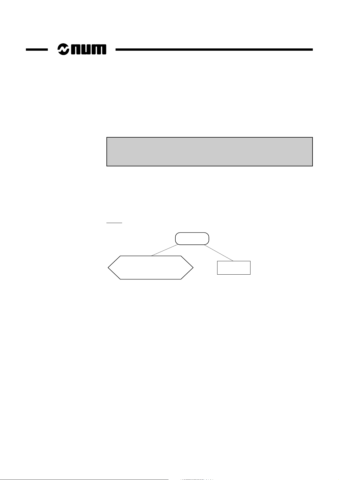
NUM 1020/1040/1060 Documentation Structure

NUM

T

PROGRAMMING

MANUAL

Volume 1
Volume 2

938820

NUM

AUTOMATIC

CONTROL

FUNCTION

PROGRAMMING

MANUAL LADDER

LANGUAGE

938846

NUM

SYNCHRONISATION

OF TWO SPINDLES

938854

User Documents

These documents are designed for use of the CNC.

Forword

Foreword

NUM

M/W

OPERATOR

MANUAL

938821

OPERATOR

Integrator Documents

NUM
1060

INSTALLATION

AND

COMMISSIONING

MANUAL

938816

INSTALLATION

COMMISSIONING

NUM

T

MANUAL

938822

NUM

M

PROGRAMMING

MANUAL

Volume 1
Volume 2

938819

These documents are designed for setting up the CNC on a machine.

NUM

1020/1040

AND

MANUAL

938938

NUM

PARAMETER

MANUAL

938818

NUM

G

CYLINDRICAL

GRINDING

PROGRAMMING

MANUAL

938930

NUM

DYNAMIC

OPERATORS

938871

NUM

PROCAM

DESCRIPTION

LANGUAGE

938904

NUM

G

CYLINDRICAL

GRINDING

COMMISSIONING

MANUAL

938929

NUM

H/HG

GEAR

CUTTING AND

GRINDING

MANUAL

938932

NUM

GS

SURFACE

GRINDING

MANUAL

938945

en-938872/2 7

Special Programming Documents

NUM

PROFIL

FUNCTION

OPERATING

MANUAL

938937

These documents concern special numerical control programming applications.

NUM

SUPPLEMENTARY

PROGRAMMING

MANUAL

938872

NUM

GS

PROCAM GRIND

INTERACTIVE

PROGRAMMING

938953

NUM

M

PROCAM MILL

INTERACTIVE

PROGRAMMING

MANUAL

938873

NUM

G

PROCAM GRIND

INTERACTIVE

PROGRAMMING

938931

NUM

T

PROCAM TURN

INTERACTIVE

PROGRAMMING

MANUAL

938874

NUM

DUPLICATED

AND

SYNCHRONISED

AXES

938875

8 en-938872/2

Supplementary Programming Manual

Manual Contents

Presentation of the commands used for structured programming of branches and
loops.

CHAPTER 1

STRUCTURED

PROGRAMMING

Forword

CHAPTER 2

READING THE
PROGRAMME

STATUS ACCESS

SYMBOLS

CHAPTER 3

STORING

DATA IN

VARIABLES

L900 TO L951

Presentation of the symbols giving visibility into the programmed functions and
programme context during call of a cycle by a G function.

How to store values related to the arguments or functions programmed in variables
L900 to L951 when calling a cycle by a G function.

en-938872/2 9

CHAPTER 4

CREATING AND

MANAGING

SYMBOLIC

VARIABLE TABLES

CHAPTER 5

CREATING

SUBROUTINES

CALLED BY

G FUNCTIONS

How to create and manage symbolic variable tables for storing functions and cutting
paths.

How to create subroutines called by G functions.

How to specify tool paths by polynomials.

CHAPTER 6

POLYNOMIAL

INTERPOLATION

CHAPTER 7

COORDINATE

CONVERSIONS

10 en-938872/2

Coordinate conversions using a square matrix.

CHAPTER 8

RTCP

FUNCTION

Forword

Possibility of controlling the movements of a machine to position the tool with respect
to the part and pivot it around its centre.

Possibility of controlling the N/M AUTO axes while the other machine axes follow a
programmed path.

CHAPTER 9

N/M AUTO

FUNCTION

APPENDIX A

TABLE OF

STRUCTURED

PROGRAMMING

COMMANDS

APPENDIX B

Presents the structured programming commands in table form.

Presents the symbolic variable management commands in table form.

TABLE OF

SYMBOLIC

VARIABLE

MANAGEMENT

COMMANDS

en-938872/2 11

APPENDIX C

TABLE OF

PROGRAMME

STATUS ACCESS

SYMBOLS

APPENDIX D

TABLE OF

SYMBOLS
STORED IN
VARIABLES

L900 TO L951

Presents the programme status access symbols in table form:

- G function addressing,

- M function addressing,

- addressing a list of bits,

- addressing a value,

- addressing a list of values.

Presents lists of symbols stores in variables L900 to L951 in table form.

- Symbols stored in variables L900 to L925.

- Symbols stored in variables L926 to L951.

12 en-938872/2

Using the Supplementary Programming Manual

Syntax Conventions

The command lines (blocks) used in programming include commands, symbols,
variables, functions and/or arguments.

A particular syntax is used for each of the elements described herein. The applicable
syntax rules describe how to write the programme blocks.

Certain syntaxes are given on one or more lines. Writing is simplified by use of the
following conventions:

- the functionality(ies) to which the syntax relates is (are) highlighted by the use of
bold face characters,

- «..» or lower case letters after one or more capital letters, addresses or signs
replace a numerical value (e.g. N..),

- the ellipsis «...» replaces a character or address string similar to that preceding it
in the block (e.g. [Symb1]/[Symb2]...),

- «xx» after one or more address letters replaces alphanumeric characters (e.g.
[.IBxx(i)]),

- «xxx» after an address letter replaces numerical values (e.g. Gxxx).

Forword

Examples

Syntax for creating a symbolic variable table

P.BUILD [TAB(7,NB)] H.. N.. +n N..+n

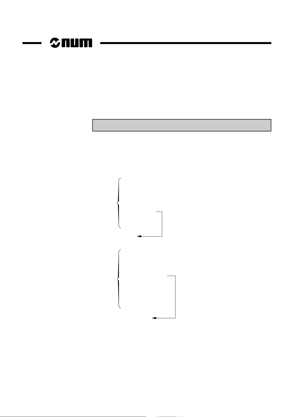
Syntax of a «repeat until» loop and its graphic representation

REPEAT

(instructions)

UNTIL (condition)

Repeat

Instructions

Until

condition

en-938872/2 13

Index

Questionnaire

Agencies

The index at the end of the volume gives access to information by keywords.

To help us improve the quality of our documentation, we request you to return the
questionnaire at the end of the volume.

The list of NUM agencies is given at the end of the volume.

14 en-938872/2

Structured Programming

1 Structured Programming

1.1 General 1 - 3

1.1.1 Commands Used in Structured Sequences 1 - 3

1.1.2 General Syntax Rules 1 - 3

1.1.3 Nesting and Branches 1 - 5

1.2 Structured Programming Commands 1 - 6

1.2.1 Condition Graph 1 - 6

1.2.2 Instruction Execution Conditions 1 - 7

1.2.3 REPEAT UNTIL Loops 1 - 8

1.2.4 WHILE Loops 1 - 9

1.2.5 Loops with Control Variable 1 - 10

1.2.6 Exiting the Loop 1 - 12

1.3 Example of Structured Programming 1 - 13

1

en-938872/2 1 - 1

1 - 2 en-938872/2

1.1 General

Structured Programming

The system provides the possibility of programming structured branches and loops,
making the programmes easier to read and simplifying the programming of complex
part programmes.

The programming tools described in this chapter are used to create subroutines
called by G functions (see Chapter 5).

A structured sequence always begins and ends with keywords.
It begins with one of the following keywords:

IF
REPEAT
WHILE
FOR

1

It ends with:
ENDI for IF
UNTIL for REPEAT
ENDW for WHILE
ENDF for FOR

The word ELSE can be interposed between the words IF and ENDI.

1.1.1 Commands Used in Structured Sequences

- Conditional execution of instructions: IF, THEN, ELSE, ENDI

- Repeat until loops: REPEAT, UNTIL

- While loops: WHILE, DO, ENDW

- Loops with control variables: FOR, TO, DOWNTO, BY, DO, ENDF

- Exit from a loop: EXIT

1.1.2 General Syntax Rules

The words IF, REPEAT, WHILE, FOR, ENDI, UNTIL, ENDW and ENDF must be the
first words in a block (no sequence number).

The words IF, REPEAT, THEN, ELSE, UNTIL, WHILE, DO and DOWNTO must
always be followed by a space, e.g.:

WHILEL0 <3 is not recognised by the system. The required syntax is WHILE L0 <3.
The words DO and THEN must immediately follow the condition. Alternately, if these

two words are not located on the same line as the words IF, WHILE and FOR, they
must be the first words on the next line.

en-938872/2 1 - 3

Blocks with sequence numbers (N..) are allowed in loops.
Blocks beginning with the words ENDI, ENDW, ENDF, EXIT or UNTIL must not

include ISO programming functions.
One of words DO, THEN or ELSE can be followed by ISO programming functions in

a same block.
Example:

WHILE L1 < 3 DO G91 X12

or

WHILE L1 < 3
DO G91 X12

The following sequence is refused:

WHILE L0 < 3 G91 X10
DO

Not allowed in a
conditional instruction

1 - 4 en-938872/2

1.1.3 Nesting and Branches

Structured Programming

Nesting

Fifteen structured nesting levels are possible independently of subroutine calls by
function G77 ...

Example:

First nesting level Second nesting level Third nesting level

IF

IF

REPEAT

UNTIL

ENDI

ENDI

Branches

Programming of a conditional or unconditional branch by G79 ... is allowed in a
structured sequence, but must branch to the lowest nesting level of the current
programme or subroutine.

Example:

1

%1 %2
IF G79 N100

WHILE REPEAT

G79 N100

good

IF
G77 H2 G79 N100
G79 N50
G79 N30

bad
bad

G79 N50

ENDI
N30 N50

ENDW UNTIL

N50 N100
ENDI
N100
M02

good

good
bad

en-938872/2 1 - 5

1.2 Structured Programming Commands

1.2.1 Condition Graph

A condition must follow one of words IF, WHILE or UNTIL and must be located in the
same block. If the block contains limits and a possible increment, they must follow
the word FOR.

Condition Graph

<
>

Parameters

Variables

Variables: All the variables used in parametric programming:

L variables, E parameters and symbolic variables.

Expression: Sequence of parameters and immediate values connected by symbols

+, -, *, /, !, & (see Chapter 6 of the Programming Manual). The operations
are calculated in sequence from left to right.

=

(Expression)

and

or

1 - 6 en-938872/2

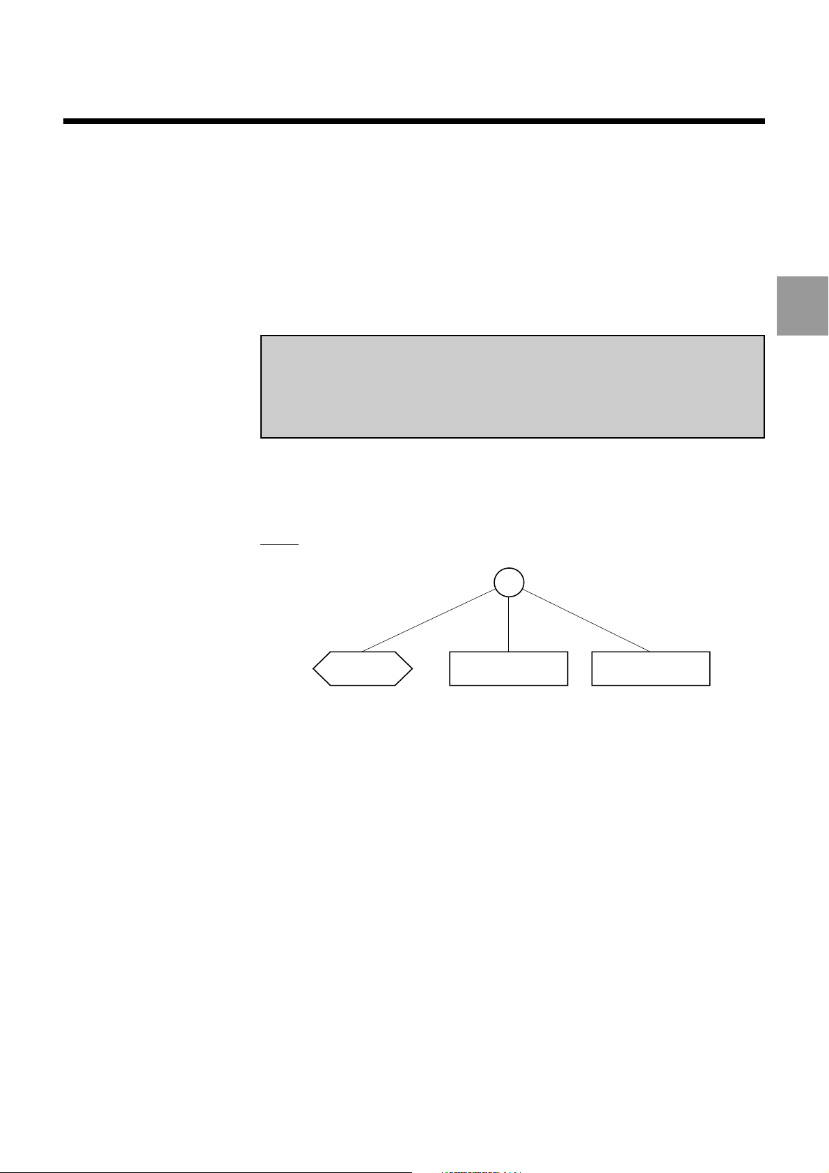
1.2.2 Instruction Execution Conditions

Structured Programming

Syntax

IF(condition) THEN

(instructions 1)

ELSE

(instructions 2)

ENDI

If the condition is true, «instructions 1» are executed. Else, «instructions 2» are
executed.

The word ELSE is optional.
Graph

IF

Condition

THEN
instructions 1

ELSE
instructions 2

1

Example

IF E70000> 100 AND E70000 <200 THEN

G77 H100
ELSE

G77 H500
ENDI

The word THEN may be programmed at the beginning of the next block and followed
by the functions to be executed.

Example:

IF L4 < 8
THEN L6 = L2+1 XL6
ENDI

en-938872/2 1 - 7

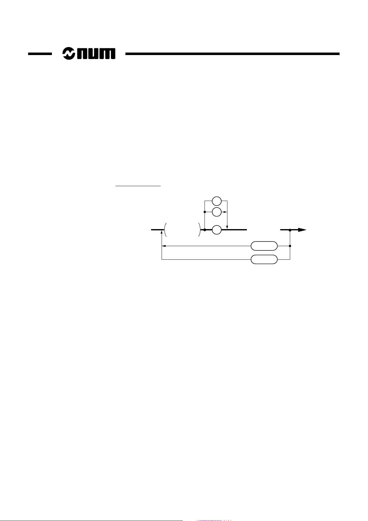
1.2.3 REPEAT UNTIL Loops

Syntax

The instructions are executed repetitively until the condition becomes true.
Even if the condition is true at the beginning, the instructions are executed once.

Graph

Example

Wait for a correct answer

REPEAT

(instructions)

UNTIL (condition)

Repeat

Untilinstructions

REPEAT

$ EXIT FROM THE PROGRAMME (Y/N) ?

[ANSWER]= $
UNTIL [ANSWER] = 14 OR [ANSWER] = 25

The answer «Y» returns the value 25
and the answer «N» returns the value
14 (ranks of the letters Y and N in the
alphabet)

1 - 8 en-938872/2

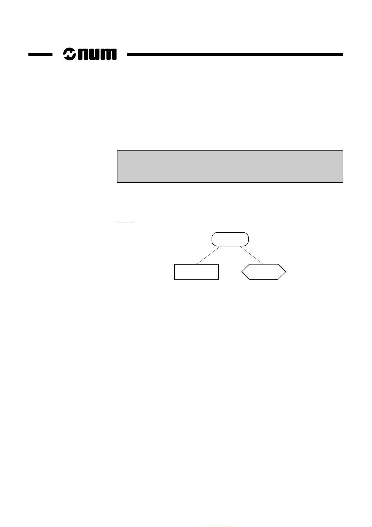
1.2.4 WHILE Loops

Structured Programming

Syntax

WHILE (condition) DO

(instructions)

ENDW

The instructions are executed while the condition remains true. Unlike REPEAT
UNTIL loops, the instructions are not executed if the condition is false at the
beginning.

Graph

While

condition

The word DO may be programmed at the beginning of the next block and followed
by the functions to be executed.

Example:

instructions

1

WHILE (condition)
DO XL6
ENDW

en-938872/2 1 - 9

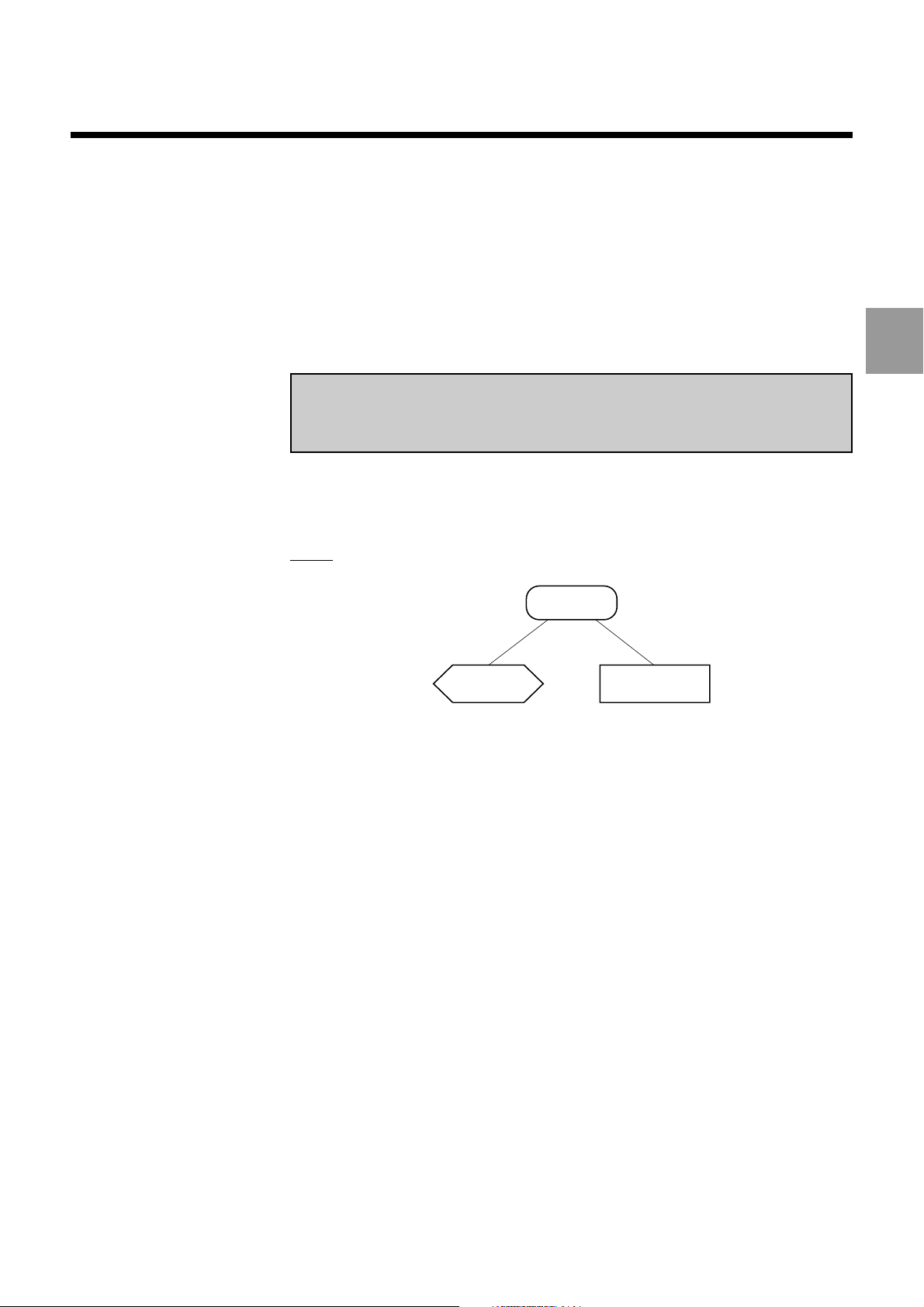
1.2.5 Loops with Control Variable

Syntax

FOR (variable) = (expression 1) TO/DOWNTO (expression 2) BY (value) DO

(instructions)

ENDF

The instructions are executed for «variable = expression 1». Then «variable» is
incremented (TO) or decremented (DOWNTO) by «value» before the «instructions»
are executed again, and the process is continued until «variable» is equal to
«expression 2».

The word «BY» is optional.
Graph

Variable = expression 1

to expression 2

by ± value

For

instructions

1 - 10 en-938872/2

The variable can be:

- an L programme variable,

- a symbolic variable,

- a parameter E80000, E81000 or E82000 (be careful about stopping computations

for L100 to L199, Exxxxx and the symbolic variables).

The expressions are positive or negative integers. The system rounds them off (down
to 0.5 and up above 0.5).

Structured Programming

With TO, the loop continues to be executed as long the current value of the variable
is less than or equal to the final value (incrementing of the variable).

With DOWNTO, the loop continues to be executed as long the current value is higher
than or equal to the final value (decrementing of the variable).

The value of BY is incremented or decremented from the variable each cycle (the
default value of Y is equal to 1).

BY must always have a positive value. If the value of BY is negative, functions TO
and DOWNTO are reversed.

Example

Resetting the tool data

FOR L1=1 TO 20
DO
L2=56000+L1
EL2=0
ENDF

1

en-938872/2 1 - 11

1.2.6 Exiting the Loop

Syntax

The EXIT instruction is used to exit from an iteration loop (FOR, WHILE or REPEAT)
and go to the next higher nesting level, ignoring any subsequent IF functions.

The word EXIT is used only in IF loops.

Example

Current

loop

EXIT

REPEAT
(instructions)
IF (condition) THEN
(instructions)
ELSE
EXIT
ENDI
UNTIL (condition)

(continued)

WHILE (condition) DO

REPEAT
IF (condition) THEN
(instructions)
IF (condition) THEN

Current

loop

EXIT
ENDI
(instructions)
ENDI

UNTIL (condition)

(instructions)
ENDW

1 - 12 en-938872/2

1.3 Example of Structured Programming

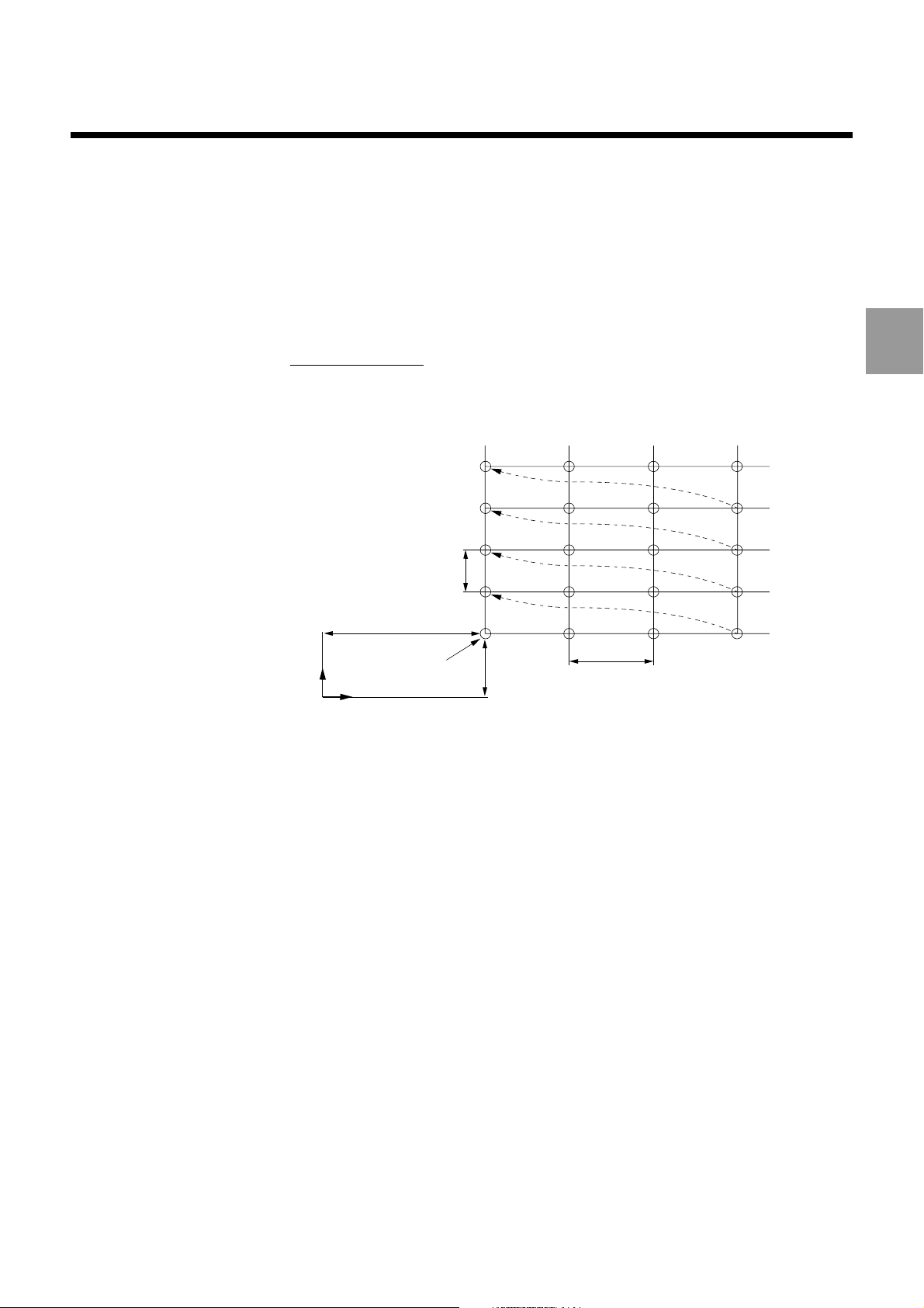
L10

L11

L1

Y

L0

Pattern

start point

X

Hole drilling pattern
L2 = number of holes in X
L3 = number of holes in Y

Structured Programming

1

en-938872/2 1 - 13

%20
$ X START:
L0=$
$ Y START:
L1=$
$ X STEP:
L10=$
$ Y STEP:
L11=$
L4=0
WHILE L4 <> 25 DO

Test for answer yes: Y

REPEAT $ NUMBER OF POINTS IN X:

L2=$

UNTIL L2>0

Test for number of columns greater
than 0

REPEAT $ NUMBER OF POINTS IN Y:

L3=$

UNTIL L3>0

Test for number of rows greater than 0

REPEAT $ PATTERN OF POINTS IN X:

$=L2
$+ /Y:
$=L3
$+ OK (Y/N) :
L4=$

UNTIL L4=14 OR L4=25

Wait for answer: N (no) or Y (yes)

ENDW
$
N.. G00 G52 XO Z0
N.. T1 D1 M06
N..
FOR L5=1 TO L3 DO

Loop on rows

$ ROW POSITION:

$=L5

XL0 L6=L5-1

L11+L1 YL6

*

G00 Z0

FOR L4=1 TO L2 DO

Loop on columns

$ DRILL THE ROW POINT:
$=L5
$+COLUMN:
$=L4
L6=L4-1*L10+L0 XL6
G01 Z-10 F50
G00 Z0

ENDF
ENDF
N..
M02

1 - 14 en-938872/2

Reading the Programme Status Access Symbols

2 Reading the Programme Status Access Symbols

2.1 General 2 - 3

2.2 Symbols for Accessing the Data of the Current Block 2 - 3

2.2.1 Symbols Addressing Boolean Values 2 - 3

2.2.1.1 Addressing G Functions 2 - 4

2.2.1.2 Addressing of M Functions 2 - 4

2.2.1.3 Addressing a List of Bits 2 - 6

2.2.2 Symbols Addressing Numerical Values 2 - 8

2.2.2.1 Addressing a Value 2 - 8

2.2.2.2 Addressing a List of Values 2 - 9

2.3 Symbols Accessing the Data of the Previous Block 2 - 11

2

en-938872/2 2 - 1

2 - 2 en-938872/2

2.1 General

Reading the Programme Status Access Symbols

The programming tools described in this chapter are required for creating subroutines
called by G functions (see Chapter 5).

The programme status access symbols give visibility into the functions programmed
in a block used to call a machining cycle by a G function. They also give information
on the part programme context when the call is made.

These symbols are used to read the modal data in the current block.
These read-only symbols are accessible by parametric programming.
These symbols can be:

- symbols to access the data in the current block,

- symbols to access the data in the previous block.
Each symbol addresses a data item or list of data items with the form of a one-

dimensional array or table.

2.2 Symbols for Accessing the Data of the Current Block

The symbols can be:

- symbols addressing Boolean values,

- symbols addressing numerical values.

General Syntax

Variable = [•symbol(i)]

Variable L programme variable, symbolic variable [symb], E

parameter.

2

[•symbol(i)] Symbol between square brackets, preceded by a

decimal point, possibly followed by an index (i).

2.2.1 Symbols Addressing Boolean Values

The symbols addressing Boolean values associated with programmed functions are
used to determine whether the functions are active or not.

The Boolean values are defined by 0 or 1.

en-938872/2 2 - 3

2.2.1.1 Addressing G Functions

[•BGxx] G function addressing.

The symbol [•BGxx] is used to determine whether the G functions specified by xx are
enabled or inhibited, e.g.:
[•BGxx]=0: function Gxx inhibited
[•BGxx]=1: function Gxx enabled

List of G Functions

[•BG00] [•BG01] [•BG02] [•BG03] [•BG17] [•BG18] [•BG19]
[•BG20] [•BG21] [•BG22] [•BG29] [•BG40] [•BG41] [•BG42]
[•BG70] [•BG71] [•BG80] [•BG81] [•BG82] [•BG83] [•BG84]
[•BG85] [•BG86] [•BG87] [•BG88] [•BG89] [•BG90] [•BG91]
[•BG93] [•BG94] [•BG95] [•BG96] [•BG97]

2.2.1.2 Addressing of M Functions

[•BMxx] M functions addressing.

The symbol [•BMxx] is used to determine whether the M functions specified by xx are
enabled or inhibited, e.g.:
[•BMxx]=0: function Mxx inhibited
[•BMxx]=1: function Mxx enabled

2 - 4 en-938872/2

List of M Functions

[•BM03] [•BM04] [•BM05] [•BM07] [•BM08] [•BM09] [•BM10] [•BM11]
[•BM19] [•BM40] [•BM41] [•BM42] [•BM43] [•BM44] [•BM45] [•BM48]
[•BM49] [•BM62] [•BM63] [•BM64] [•BM65] [•BM66] [•BM67] [•BM68]
[•BM69] [•BM997] [•BM998] [•BM999]

Reading the Programme Status Access Symbols

Example

%100
N10 G00 G52 Z0 G71
N..
N40 G97 S1000 M03 M41
N50 M60 G77 H9000
N..
N350 M02

%9000
VAR
[GPLAN] [MGAMME] [MSENS] [GINCH] [GABS]
[XRETOUR] [YRETOUR] [ZRETOUR]
ENDV

Tool check subroutine call

2

$ CONTEXT SAVE
N10 [GPLAN]=17
[GPLAN]=18
[GPLAN]=19
N20 [MGAMME]=40
[MGAMME]=41
N30 [MSENS]=03
[MSENS]=04
[MENS]=05
N40 [GINCH]=70
[GINCH]=71
N50 [GABS]=90
[GABS]=91
[XRETOUR]=E70000
[YRETOUR]=E71000
[ZRETOUR]=E72000
N60 G90 G70 G00 G52 Z0
N70 G52 X100 Y100 M05
N80 G52 G10 Z-500
N90 G52 Z0
N100 G52 Z [ZRETOUR]
N110 G52 X [XRETOUR]
N120 G52 Y [YRETOUR]
G[GPLAN] M[MGAMME]
M[MSENS] G[GINCH] G[GABS]

[•BG17]

*

[•BG18]+[GPLAN]

*

[•BG19]+[GPLAN]

*

[•BM40]

*

[•BM41]+[MGAMME]

*

[•BM03]

*

[•BM04]+[MSENS]

*

[•BM05]+[MSENS]

*

[•BG70]

*

[•BG71]+[GINCH]

*

[•BG90]

*

[•BG91]+[GABS]

*

Interpolation plane

Speed range

Direction of rotation

Inches

Absolute

Tool check position

Return to Z position

Restore context

en-938872/2 2 - 5

2.2.1.3 Addressing a List of Bits

[•IBxx(i)] Addressing a list of bits.

The symbol [•IBxx(i)] addresses a list of bits corresponding to the items specified by
xx.

The values are Boolean, i.e. 0 or 1.
The index (i) defines the rank of the element in the list.
[•IBX(i)] List of axes programmed in the current block.

Index i = 1 to 11.
This nonmodal list can remain stored and be read by parametric
programming if the system is in state G999.
i = 1: X axis
i = 2: Y axis
i = 3: Z axis
i = 4: U axis
i = 5: V axis
i = 6: W axis
i = 7: A axis
i = 8: B axis
i = 9: C axis
i = 10: in G21: Y axis address index 10

in G22: Z axis address index 10

i = 11: in G21: X axis address index 11

in G22: Y axis address index 11

2 - 6 en-938872/2

[•IBX1(i)] List of axes programmed from the beginning of the programme to

the current block.
Index i = 1 to 9: Same as list of axes programmed in the current
block (see [•IBX(i)]).
The axes programmed with respect to the measurement origin
(G52) are cancelled in this list, but are included in it again if
programming is resumed with respect to the programme origin.

[•IBX2(i)] List containing the last axes programmed (primary axes X Y Z or

secondary axes U V W).
Index i = 1 to 6. Except for axes A, B and C, the list is the same
as for the axes programmed in the current block (see [•IBX(i)]).
Programming an axis in a group cancels the equivalent axis in
other group. For instance, programming axis V resets the bit
relative to X and sets the bit for V.

Reading the Programme Status Access Symbols

[•IBXM(i)] Mirroring of the axes. The bit is set to indicate mirroring and is

reset to indicate no mirroring.
Index i = 1 to 9: same as the list of axes programmed in the
current block (see [•IBX(i)]).

[•IBI(i)] List of arguments I, J and K programmed in the current block.

Index i = 1 to 5.
List modal only in state G999.
i = 1: argument I
i = 2: argument J
i = 3: argument K
i = 4: in G21: J component address index 4

in G22: K component address index 4

i = 5: in G21: I component address index 5

in G22: J component address index 5

[•IBP(i)] List of arguments P, Q and R programmed in the current block.

Index i = 1 to 3.
List modal only in state G999.
i = 1: argument P
i = 2: argument Q
i = 3: argument R

2

en-938872/2 2 - 7

2.2.2 Symbols Addressing Numerical Values

The symbols addressing numerical values are used to read the modal data of the
current block.

2.2.2.1 Addressing a Value

[•Rxx] Addressing a value.

The symbol [•Rxx] is used to address a value corresponding to the elements specified
by xx.

[•RF] Feed rate

(units as programmed by G93, G94 or G95).

[•RS] Spindle speed

(G97: format according the spindle characteristics declared in

machine parameter P7).
[•RT] Tool number.
[•RD] Tool correction number.
[•RN] Number of the last sequence (block) encountered.

If the block number is not specified, the last numbered block is

analysed.
[•RED] Angular offset.
[•REC] Spindle orientation (milling).
[•RG4] Dwell time programmed (G04 F..).

This nonmodal function may however remain stored. Its value

can therefore be read if the system is in state G999 or G998.
[.RG80] Number of the calling function in a subroutine called by G

function.

In a subroutine called by G function, the number of the calling

function is addressed by [.RG80] (in state G80, its value is zero).
[•RNC] Value of NC (spline curve number).
[•RDX] Tool axis orientation.

Defined by the following signs and values:

+1 for G16 P+ +2 for G16 Q+ +3 for G16 R+

-1 for G16 P- -2 for G16 Q- -3 for G16 R-

[•RXH] Nesting level of the current subroutine.

1: main programme

2: first nesting level

3: second nesting level, etc. (8 possible nesting levels)

2 - 8 en-938872/2

2.2.2.2 Addressing a List of Values

[•IRxx(i)] Addressing a list of values.

Reading the Programme Status Access Symbols

The symbol [•IRxx(i)] is used to address a list of values corresponding to the elements
specified by xx.

Index (i) defines the rank of the element in the list.
[•IRX(i)] Values of the dimensions programmed on the axes.

Index i = 1 to 11.

i = 1: value of X

i = 2: value of Y

i = 3: value of Z

i = 4: value of U

i = 5: value of V

i = 6: value of W

i = 7: value of A

i = 8: value of B

i = 9: value of C

i = 10: in G21: Y axis address index 10

in G22: Z axis address index 10

i = 11: in G21: X axis address index 11

in G22: Y axis address index 11

[•IRTX(i)] Values of the offsets programmed on the axes.

Index i = 1 to 9, same as the values of the dimensions

programmed on the axes (see [•IRX(i)]).
[•IRI(i)] Values of arguments I, J and K. Index i = 1 to 5.

i = 1: value of I

i = 2: value of J

i = 3: value of K

i = 4: in G21: J component address index 4

in G22: K component address index 4

i = 5: in G21: I component address index 5

in G22: J component address index 5

2

[•IRP(i)] Values of arguments P, Q and R. Index i = 1 to 3.

i = 1: value of P

i = 2: value of Q

i = 3: value of R
[•IRH(i)] Numbers of current programmes or subroutines or lower nesting

levels.

Index i = 1 to n subroutine.

i = 1: addresses the main programme

i = 2: addresses the subroutine called by the main programme

i = 3: addresses the next subroutine, etc. (8 possible nesting

levels)

en-938872/2 2 - 9

[•IRDI(i)] Values defining the origin of the programmed angular offsets

(G59 I.. J.. K..). Index i = 1 to 3.

i = 1: value of I

i = 2: value of J

i = 3: value of K

2 - 10 en-938872/2

Reading the Programme Status Access Symbols

2.3 Symbols Accessing the Data of the Previous Block

The same data can be accessed in the previous block as in the current block (see 2.2).
The same symbols are used, but are preceded by two decimal points (instead of one).

The symbols can be:

- symbols addressing Boolean values, or

- symbols addressing numerical values.
The symbols are used to read the modal data of the previous block.
These data are those of the last executable previous block (or possibly the last block

executed).
This addressing is used only when execution of the current block is suspended by

programming function G999.

2

General Syntax

Variable = [••symbol(i)]

Variable L programme variable, symbolic variable [symb], E

parameter.

[••symbol(i)] Symbol between square brackets, preceded by two

decimal points, possibly followed by an index (i).

en-938872/2 2 - 11

2 - 12 en-938872/2

Storing Data in Variables L900 to L951

3 Storing Data in Variables L900 to L951

3.1 General 3 - 3

3.2 Storing F, S, T, H and N in Variables L900 to L925 3 - 3

3.3 Storing EA to EZ in Variables L926 to L951 3 - 4

3.4 Symbolic Addressing of Variables L900 to L951 3 - 4

3

en-938872/2 3 - 1

3 - 2 en-938872/2

3.1 General

Storing Data in Variables L900 to L951

The programming tools described in this chapter are necessary for creating subroutines
called by G functions (see Chapter 5).

Certain arguments or functions may have different meanings in the machining cycles
programmed. Status symbols [•IBE0(i)] and [•IBE1(i)] are used to detect their
presence in blocks including a G function calling a subroutine.

It is up to the subroutine to correctly address these arguments or functions according
to their meanings and to store their values in variables L900 to L951.

The bits of [•IBE0(i)] and [•IBE1(i)] (each equal to 0 or 1) are accessible for read by
parametric programming.

3.2 Storing F, S, T, H and N in Variables L900 to L925

Storing F, S and T

Status symbol [•IBE0(i)] consisting of a list of bits is used to detect programming of
F, S or T in blocks including a function Gxxx.

Index (i): from 1 to 26 for addresses A to Z.
Addressing the status symbol:

- bit [•IBE0(6)] is set if F is programmed,

- bit [•IBE0(19)] is set if S is programmed,

- bit [•IBE0(20)] is set if T is programmed.
The values of F, S and T are stored in the following variables (L900 to L925):

- F in L905,

- S in L918,

- T in L919.

Storing H and N

H and N can only be stored when not preceded by functions G75, G76, G77 or G79
related to them for ISO programming.

3

A second N (following the first N and defining the last call sequence of a subroutine
N.. to N..) is stored in variable L914 (this N can in no case be the block number
programmed at the start of the sequence).

Addressing the status symbol:

- bit [•IBE0(8)] is set if H is programmed,

- bit [•IBE0(14)] is set if the first N is programmed,

- bit [•IBE0(15)] is set if the second N is programmed.

en-938872/2 3 - 3

The values of H and N are stored in the following variables:

- H in L907,

- first N in L913,

- second N in L914.

3.3 Storing EA to EZ in Variables L926 to L951

The values of EA to EZ to be stored in variables L926 to L951 are defined by two
alphabetic characters:

- the first is the letter E,

- the second is a letter between A and Z.
Status symbol [•IBE1(i)] consisting of a list of 26 bits is used to detect the presence

of functions EA to EZ in blocks including a function Gxxx (i = alphabetic index of the
second letter after E).

Addressing the status symbol:

- bit [•IBE1(1)] addresses the bit corresponding to EA,

- bit [•IBE1(2)] addresses the bit corresponding to EB, and so forth down to ...,

- bit [•IBE1(26)] addresses the bit corresponding to EZ.
The values are stored in the following variables (L926 to L951):

- EA in L926,

- EB in L927, and so forth down to ...,

- EZ in L951.

3.4 Symbolic Addressing of Variables L900 to L951

Variables L900 to L925 and L926 to L951 in either the left-hand or right-hand side of
an expression can be addressed by alphabetic symbols preceded by the character
«‘» (apostrophe).

Variables L900 to L925

L900 to L925 can be addressed by symbols ‘A to ‘Z.
Example:
‘C = ‘A + ‘B is equivalent to L902 = L900 + L901

Variables L926 to L951

L926 to L951 can be addressed by symbols ‘EA to ‘EZ respectively.
(‘EA = L926, ‘EB = L927, etc. up to ‘EZ = L951).
Example:
‘A = ‘B - ‘EA / ’EZ is equivalent to L900 = L901 - L926 / L951.

3 - 4 en-938872/2

Creating and Managing Symbolic Variable Tables

4 Creating and Managing Symbolic Variable Tables

4.1 Creating Symbolic Variable Tables 4 - 3

4.1.1 Defining a Table 4 - 3

4.1.2 Table Dimensions 4 - 3

4.1.3 Initialising Variables and Tables 4 - 5

4.1.4 Creating Tables for Storing Profiles 4 - 6

4.1.5 Data That Can Be Stored in a Table 4 - 7

4.2 Symbolic Variable Management Commands 4 - 8

4.2.1 Storing a Profile 4 - 8

4.2.2 Storing a Profile Interpolated in the Plane 4 - 11

4.2.3 Offsetting an Open Profile and Updating
the Table 4 - 13

4.2.4 Redefining a Profile According to the Tool
Relief Angle 4 - 15

4.2.5 M Functions and/or Axes Enabled or
Inhibited. Setting or Resetting Bits 4 - 18

4.2.6 Searching the Stack for Symbolic
Variables 4 - 20

4.2.7 Providing a List of Symbolic Variables 4 - 21

4.2.8 Copying Blocks or Entries from One Table
into Another Table 4 - 22

4.2.9 Indirect Addressing of Symbolic Variables 4 - 27

4.2.10 Programming Examples 4 - 28

4

en-938872/2 4 - 1

4 - 2 en-938872/2

Creating and Managing Symbolic Variable Tables

The programming tools described in this chapter are used to create subroutines
called by G functions (see Chapter 5).

4.1 Creating Symbolic Variable Tables

The rules for writing symbolic variables used when creating tables are the same as
those defined for parametric programming (see Chapter 7 of the Programming
Manual).

4.1.1 Defining a Table

A table is declared as a symbolic variable between the words VAR and ENDV.
A table is defined by including its dimensions between brackets after the last

character of the symbolic variable.
For tables with several dimensions, the dimensions are separated by commas «,» or

semicolons «;».

Syntax

VAR

[TABLn(a,b,c ...)]

ENDV

VAR Declaration of symbolic variables.
[TABLn(a,b,c...)] TABLn: table name in the stack.

(a,b,c ...) : table dimensions.

ENDV End of symbolic variable declaration.
Example of table definitions

VAR
[TABL1(10)] [TABL2(2,5,3)]
ENDV

For table 2 [TABL2] above, the number of entries reserved equals:
2 x 5 x 3 = 30 entries, i.e. 5 groups of 2 then 3 groups of 10.

4

4.1.2 Table Dimensions

Tables can have from one to four dimensions.
For tables with one dimension:

- the value of a dimension must be between 1 and 65535.

en-938872/2 4 - 3

For tables with 2, 3 or 4 dimensions:

- the value of a dimension must be between 1 and 255.
The dimensions must be declared as immediate values or declared symbolic

variables.
Example:

[VAR1] = 10
[VAR] = [TAB1 (VAR1,5)]

Symbolic variables are real values.
Table indexes are immediate values or symbolic variables.
A dimension cannot be defined using:

- L programme variables,

- E external parameters.
Example:
If symbolic variable [TAB(L0,3)] is programmed, it is not programme variable L0 but

symbolic variable [L0] that is searched for.
The table indexes can be additions or subtractions of values or symbolic variables.
Example:

is equivalent to:

[TAB1 (10,5)]

VAR [IX] [COSX] [SINX] [NBT] = 4
[TABL(2,NBT)] = 0, 0, 10, 5, 20, 8, 30, -2
ENDV
FOR [IX] = 1 TO [NBT] -1 DO
[COSX] = [TABL(1,IX+1)] - [TABL(1,IX)]
[SINX] = [TABL(2,IX+1)] - [TABL(2,IX)]

L0 = [COSX]

[COSX] L0 = [SINX]

*

[SINX] + L0

*

[COSX] = [COSX] / RL0 [SINX] = [SINX] / RL0
X [TABL(1,IX+1)] Y [TABL(2,IX+1)]
ENDF

4 - 4 en-938872/2

Structure of tables with several dimensions
The entries for the first dimension are located first in the declaration, then multiplied

by the number of entries of the second dimension. The result is then multiplied by the
number of entries of the following dimension and so forth.

4.1.3 Initialising Variables and Tables

The values are initialised with a default value of zero.
Initialising with other values is made by declaring the character = followed by the initial

value(s) separated by commas «,».
The initial values can be declared in several blocks. In this case, the character = is

repeated before the value(s) defined in the next block.
Example:

VAR [NTB] = 4 [TABLE(2,NTB)] = 3,6
= 10,1,8,2,6,6
ENDV

Creating and Managing Symbolic Variable Tables

4

If

L0= [TABLE(2,3)]

L0= 2 (ie. the loth digit)

Storage in the memory

TABLE (1.1) = 3
TABLE (2.1) = 6

TABLE (1.2) = 10

4 x

Second

dimension

2

2

2

2

First

dimension

NBT = 4

(2.2) = 1
(1.3) = 8
(2.3) = 2
(1.4) = 6
(2.4) = 6

en-938872/2 4 - 5

4.1.4 Creating Tables for Storing Profiles

Entry 1 Entry 2 Entry 3 Entry 4 Entry 5 etc.

First dimension

Second
dimension

(blocks)

The system offers the possibility of storing a profile written in ISO or PGP in a table
of the programme stack. The table is created as the profile blocks are read.

The programmed blocks are stored in a table with two dimensions:

- the first dimension includes all the functions to be saved in a block,

- the second dimension corresponds to the number of blocks in the profile.
The data in the table are then accessed by parametric programming.
Example:

4 - 6 en-938872/2

Creating and Managing Symbolic Variable Tables

4.1.5 Data That Can Be Stored in a Table

The following ISO programming data can be stored in tables.
G Functions

Only one G function per block can be stored.
After a change of interpolation plane in a block, the new function is stored (G17, G18

or G19 for milling, G20, G21 or G22 for turning). Otherwise, one of modal functions
G00, G01, G02 or G03 is stored.

Values of the Programmed Axes
X, Y, Z, U, V, W, A, B, C (depending on the axes declared in machine parameter P0).
The modal values programmed with the axes are stored.

Values of I, J, K, P, Q, R
The values of the functions are stored only if the functions are present in the block.

Otherwise, the value zero is stored in the corresponding entries.
Feed Rate F

The modal value related to function F is stored.
Spindle Speed S

The value of S is not stored in the table unless it is present in the block. Otherwise,
a value of zero is stored.

Tool Call T
Function T is not stored in the table unless it is present in the block. Otherwise, a value

of zero is stored.

4

en-938872/2 4 - 7

4.2 Symbolic Variable Management Commands

4.2.1 Storing a Profile

BUILD Creates a table for storing profile paths.

The BUILD function is used to store the profile in a two-dimensional table:

- the first dimension is limited to 16 entries,

- the second dimension is limited to 255 entries.

Syntax

BUILD [TAB(G / X / Y / I / J,NB)] H.. N..+n N..+n

BUILD Creation of a table for storing a profile.
TAB Table name in the stack.
G / X / Y / I / J Data types whose values are stored in the entries of the

first table dimension (16 entries maximum).

NB Name of the variable containing the number of blocks of

the second table dimension (maximum 255 blocks).

H.. Definition of the limits of the profile.
N.. N..
H.. N.. N..
N..+n N..+n
H N..+n N..+n

4 - 8 en-938872/2

Note

The BUILD function must be the first word in the block and the table name TAB must
be the second. They must be separated by at least one space.

Creating and Managing Symbolic Variable Tables

Programming the table name TAB and variable NB automatically creates a two­dimensional table.

Example:

%555 %55

N10 ... G.. ...

First block of the profile

N.. G.. ...

N.. G.. ...

BUILD [TAB(G/X/Y/I/J,NB)] H55 G.. ...

Last block of the profile

N..

Two-dimensional table created by the above programme:

- first dimension: 5 entries,

- second dimension: 4 entries (blocks).

(blocks)

NB

TAB

Allocation of Additional Entries in a Field of the BUILD Function
Additional entries can be allocated in the first table dimension if they are not initialised

by data in the blocks. In this case, the entries are declared by «0s» separated by the
character /.

Example:

..
..
..
..

4

..
..
..
..

...
...
...
...

..
..
..
..

..
..
..
..

%55
N10 ...
N..
N110

First block of the profile

N..
N..
N220

Last block of the profile

N..
BUILD [PROF1(G/X/Y/Z/0/0,NB)] N110 N220

The first table dimension includes
6 entries

4

en-938872/2 4 - 9

Declaring Entries as a List of Bits in a Field of the BUILD Function
In a symbolic variable, some of the following axes and arguments can be declared

as a list of bits:

- axes X, Y, Z, etc.,

- arguments I, J, K,

- arguments P, Q, R.
The list of bits is declared by programming one of addresses X, I or P followed by a

decimal point and the symbolic variable name in a field of BUILD.
Example:

BUILD [TAB1(G/I.Symb/R,NB)] H..

Symbolic variable [Symb] contains a sum of values. This sum is defined from the
indexes of the addressing symbols [••IBX(i)], [••IBI(i)] and [••IBP(i)], i.e.:

- 1 for index i = 1

- 2 for index i = 2

- 4 for index i = 3

- 8 for index i = 4, etc.
Therefore, the value of the variable including I, J and K of [••IBI(i)] is equal to

I-1

J-1

2

+ 2

Example:

+ 2

K-1

.

Declaration of I.Symb

VAR [LIST] = 6
ENDV
BUILD [PROF(G/X.LIST/R,NB)] N.. N..

is equivalent to the following block:

BUILD [PROF(G/Y/Z/R,NB)] N.. N..

4 - 10 en-938872/2

Creating and Managing Symbolic Variable Tables

4.2.2 Storing a Profile Interpolated in the Plane

P.BUILD Creates a table for storing the dimensions of the profile

interpolation plane.

The P.BUILD function is used to store the profile in a two-dimensional table:

- the first dimension is limited to 7 entries,

- the second dimension is limited to 255 entries.

Syntax

P.BUILD [TAB(7,NB)] H.. N..+n N..+n

BUILD Creation of a table for storing a profile.
TAB Table name in the stack.
7 Number of entries in the first dimension (maximum 7).
NB Name of the variable containing the number of blocks

(maximum 255 blocks).

H.. Definition of the limits of the profile.
N.. N..
H.. N.. N..
N..+n N..+n
H.. N..+n N..+n

Note

The P.BUILD function must be the first word in the block and the table name TAB must
be the second. They must be separated by at least one space.

4

en-938872/2 4 - 11

Defining the Seven Entries of the First Dimension with the P.BUILD Function

0

+1

0

20
20
10

10
50
20

0

20

0

0

30

0

10
20
20

10
10
50

3

NB

(blocks)

TAB

- entry 1: Type of interpolation:
value = 0 for linear interpolation,
value = -1 for clockwise circular interpolation,
value = +1 for anticlockwise circular interpolation.

- entry 2: End point, value of the dimension on the X axis.

- entry 3: End point, value of the dimension on the Y axis.

- entry 4: Position of the centre:
value on the X axis for circular interpolation, else value = 0.

- entry 5: Position of the centre:
value on the Y axis for circular interpolation, else value = 0.

- entry 6: Start point, value of the dimension on the X axis.

- entry 7: Start point, value of the dimension on the Y axis.

Example:

%70 %80
N10 G17 X10 Y10 N10 ...
P.BUILD [TAB(7,NB] H80 N110 N130 N..
N.. N..

N110 G01 X20
N120 G03 X20 Y50 I20 J30
N130 G01 X10 Y20

N.. ...

4 - 12 en-938872/2

Table TAB and variable NB create the following table with 7 entries:

Creating and Managing Symbolic Variable Tables

4.2.3 Offsetting an Open Profile and Updating the Table

R.OFF Normal offset of an open profile.

The R.OFF function is used for normal offset of a profile initially created in a table by
the P.BUILD function or a table with the same format, i.e. [Pa(7,Nb)].

After execution of the R.OFF function, the offset profile is contained in the same table
and the variable specifying the number of blocks is updated since intermediate blocks
may have been created (see Fig. 1).

Syntax

R.OFF [Pa(7,Nb)] / ±1 / R

4

R.OFF Normal offset of a profile.
Pa Table name.
7 Number of table entries.
Nb Name of the variable containing the number of blocks in

table Pa.

±1 Value = +1: right offset of the profile,

value = -1: left offset of the profile.

R Radius expressed in the same units as the dimensions.

Note

The R.OFF function must be the first word in a block.
The profile executed with the R.OFF function must be an open profile, i.e. the start

point of the profile must be different from the end point (see Fig. 2).
The R.OFF function can only operate on profiles contained in P.BUILD that do not

include alternating left and right offsets during execution.

en-938872/2 4 - 13

Creation of an Intermediate Block by the System
When the profile includes particular

paths, the system may create a
connection block.

Open contour
When the profile includes a narrowed

section, it must be sufficiently large to
allow passage of the tool. Otherwise,
the system considers the profile to be
closed.

Figure 1

R

-1 offset

Figure 2

Narrowed section > tool

Intermediate

block

4 - 14 en-938872/2

Example

%92
N..
P.BUILD [P(7,NB)] N110 N200
...
...
R.OFF [PA(7,NB)] /-1 /10

Profile offset by 10 to the left

Creating and Managing Symbolic Variable Tables

4.2.4 Redefining a Profile According to the Tool Relief Angle

CUT Elimination of the grooves or parts of groove located inside the tool

relief angle.

The CUT function applies to grooves located in the path of a plane profile created in
a table by the P.BUILD function or a table with the same format, i.e. [Pa(7,Nb)].

After execution of the CUT function, the new profile is contained in the same table and
the variable specifying the number of blocks is updated.

Syntax

CUT * [Pa(7,Nb)] / Angle

4

CUT Eliminates the grooves or parts of grooves located

within the tool relief angle.

*

Pa Table name.
7 Number of table entries.
Nb Name of the variable containing the number of blocks in

Angle Angle Relief angle in degrees.

Note

The CUT function must be the first word in the block (no sequence number).

When the character * precedes the table name, all the
grooves located within the tool relief angle are
processed.
When the character * is missing in front the table name,
only the first groove located within the tool relief angle is
processed.

table Pa.

en-938872/2 4 - 15

Review of the Angles of a Cutting Tool Defined in Plane ZX
Charac teristic angles:

- Kr: approach angle,

- εr : tool nose angle,

- a : clearance angle.

Processing of the table
The table analysis begins on the first block and ends:

- on the last block with CUT * ...,

- on the first cut with CUT ...

In the table, the profile must always be defined so that the profile start dimension on
the X axis (first block) is less than the profile end X dimension (last block).

Example:

Profile correctly defined Profile incorrectly defined

εr

Kr

a

Feed direction

4 - 16 en-938872/2

First
block

Last

block

Last
block

First

block

Creating and Managing Symbolic Variable Tables

a

,,,,,

,,,,,

,,,,,

,,,,,

a

a

When the clearance angle is negative or zero (between 0 degrees and -180 degrees),
the profile areas located below this angle are eliminated.

When the relief angle is positive (between 0 degrees and +180 degrees), the profile
areas above the angle are eliminated.

Examples:

«a» shows the areas that are eliminated.
Example 1:
Elimination of the first groove in the profile (no * in front of the variable).

CUT [PA(7,NB)] / -95

Example 2:
Elimination of the grooves or parts of grooves located on the profile (* in front of the

variable).

CUT * [PA(7,NB)] / -50

4

en-938872/2 4 - 17

4.2.5 M Functions and/or Axes Enabled or Inhibited. Setting or Resetting Bits

BSET Programming of M functions and/or one or more axes enabled.

Setting of the bits of [•IBE0(i)] and [•IBE1(i)].

BCLR Programming of M functions and/or one or more axes inhibited.

Resetting of the bits of [•IBE0(i)] and [•IBE1(i)].

Syntax

BSET [•BMxx] / [•IBX(i)] / [•IBE0(i)] / [•IBE1(i)]

BSET Enabling the programming of M functions and/or one or

more axes.

[•BMxx] / [•IBX(i)] When the system is in state G999, enabling by BSET

sets the bits of [•BMxx] and/or [•IBX(i)].

[•IBE0(i)] / [•IBE1(i)] When a subroutine is called by function Gxx, BSET also

sets the bits of [•IBE0(i)] and [•IBE1(i)].

Syntax

BCLR [•BMxx] / [•IBX(i)] / [•IBE0(i)] / [•IBE1(i)]

BCLR Inhibiting the programming of M functions and/or one or

more axes.

[•BMxx] / [•IBX(i)] When the system is in state G999, inhibiting by BCLR

resets the bits of [•BMxx] and/or [•IBX(i)].

[•IBE0(i)] / [•IBE1(i)] When a subroutine is called by function Gxx, BCLR also

resets the bits of [•IBE0(i)] and [•IBE1(i)].

4 - 18 en-938872/2

Creating and Managing Symbolic Variable Tables

Note

Functions BSET and BCLR:

- must be the first words in the block (no sequence number),

- must be separated from the list of symbols by at least one space. However, there

must be no spaces in the list of symbols,

- are followed by the list of symbols to be enabled or inhibited. The symbols are

separated by «/».

Example

In block N120, only movements X10 and Z10 are executed. The movements on the
Y and B axes and the "post M" function M05 are inhibited (see Chapter 2 for indexes
(2) and (8) corresponding to Y and B respectively).

N..
N..
N.. G999 X10 Y10 Z10 B30 M05
BCLR [•IBX(2)] / [

IBX(8)] / [

•

BM05]

•

Disabled

N120 G997

4

en-938872/2 4 - 19

4.2.6 Searching the Stack for Symbolic Variables

SEARCH Searches the stack for a symbolic variable.

Syntax

SEARCH [Symb] N..

SEARCH Searches the stack for a symbolic variable.
[Symb] Name of the symbolic variable.

When the variable searched for is found, analysis of the
block is continued.

N.. Block number to which a branch is made when the

symbolic variable is not found.

Example

%30
N..
VAR [Symb]
ENDV
N..

4 - 20 en-938872/2

%35
N..
N90 ...
SEARCH [Symb] N100
N..
N100
N..

Creating and Managing Symbolic Variable Tables

4.2.7 Providing a List of Symbolic Variables

SAVE Provides the main programme and subroutines with a list of the

symbolic variables declared in any subroutine.

Syntax

SAVE [Symb1] / [Symb2] ...

SAVE Provides the main programme and subroutines with a

list of the symbolic variables declared in any subroutine.

[Symb1] / [Symb2] ... List of symbolic variables.

4

Notes

The symbolic variables provided may be declared within subroutines at any nesting
levels.

The variables declared after SAVE must be separated by the character «/».

Example

After a return from subroutine %30, programme %10 and subroutine %20 as well as
any new subroutines can use symbolic variables [V1] and [TB(4)].

%10
N..
N.. G77 H20
N..

%20
N..
N.. G77 H30
N..

%30
N..
VAR [V1] / [TB(4)]
ENDV
N..
SAVE [V1] / [TB(4)]
N..

en-938872/2 4 - 21

4.2.8 Copying Blocks or Entries from One Table into Another Table

MOVE Copies all or part of a table into another table.

The MOVE function is used to copy tables with the following formats:

- [P(m)] : m blocks of an entry,

- [P(n,m)] : m blocks of n entries.

General Syntax

MOVE [Pj(nj,mj)],mj1,mj2 = [Pi(ni,mi)],mi1,mi2 / j1=i1 / j2=i2 /jn=in

The MOVE function provides several possibilities for copying:

- simple copying of blocks,

- partial copying of blocks,

- specification of the entries to be copied.

Syntax for Simple Copying of Blocks

MOVE [Pj(nj,mj)] = [Pi(ni,mi)]

MOVE Copies the contents of one table into another table.

During a simple copy, the two tables must have the
same format, i.e.: nj = ni and mj = mi.

4 - 22 en-938872/2

Pj Target table name.
nj,mj Entries and blocks of the target table.
Pi Source table name.
ni,mi Entries and blocks of the source table.

Creating and Managing Symbolic Variable Tables

Syntax for Partially Copying Blocks

MOVE [Pj(nj,mj)],mj1,mj2 = [Pi(ni,mi)],mi1,mi2

MOVE Copies the contents of one table into another table.
Pj Target table name.
nj,mj Entries and blocks of the target table.
mj1,mj2 Limits of target table Pj between which are copied the

blocks indexed mi1 to mi2 of the source table Pi. The
other blocks of Pj are not modified.

Pi Source table name.

4

ni,mi Entries and blocks of the source table.
mi1,mi2 Indexed limits of source table Pi.

These limits and the blocks between these two limits
are copied into table Pj between limits mj1 and mj2.

Syntax for Specifying Entries to Be Copied

MOVE [Pj(nj,mj)] = [Pi(ni,mi)] / j1=i1 / j2=i2 / jn=in

MOVE Copies the contents of one table into another table.
Pj Target table name.
nj,mj Entries and blocks of the target table.
Pi Source table name.
ni,mi Entries and blocks of the source table.
/ j1=i1 / j2=i2 / jn=in When certain entries of a table are not to be copied,

each entry to be copied must be specified with, after the
character «/», the target entry index followed by the
character «=» and the source entry index.
The value of an entry copied in the target table can be
inverted by preceding the source entry index by the sign
«-» (minus).

en-938872/2 4 - 23

Notes

The MOVE function must be the first word in the block (no sequence number).
The maximum number of blocks in a finished profile is limited to 95.
It is possible to reverse the order of a copy by reversing the start and end limit indexes

in one of the tables.
The indexes can be specified in symbolic variables.
In case of a programming error, the system returns the following error numbers:

ERROR 196 (inconsistency in index declaration),
ERROR 199 (syntax error).

Examples

MOVE simple copy of blocks
Example: Copying the contents of one table into another table.

MOVE [PB(2,3)] = [PA(2,3)]

Entries 1

Block 1
Block 2
Block 3

Target table

212

Source table

1
2

3

4 - 24 en-938872/2

Creating and Managing Symbolic Variable Tables

MOVE partial copy of blocks
Example 1: Copying part of a table into another table.

MOVE [PB(2,5)],2,5 = [PA(2,6)],1,4

4

Example 2: Copying part of a table into another table.

MOVE [PB(2,5)],2,4 = [PA(2,6)],3,5

Example 3: Reversal of the limit and block indexes when copying part of a table into
another table.

MOVE [PB(2,5)],2,5 = [PA(2,6)],4,1

en-938872/2 4 - 25

MOVE: Partial copying of blocks and specification of the entries to be copied

,,

,,

,,

,,

,,,,,

,,

,,

,,

,,

,,,,,

,,

,,

,,

,,

,,,,,

,,

,,

,,

,,

,,,,,

,,

,,

,,

,,

,,,,,

,,

,,

,,

,,

,,,,,

,,

,,

,,

,,

,,,,,

,,

,,

,,

,,

,,,,,

,,

,,

,,

,,

,,,,,

,

,,

,,

,,

,,,,,

,

,
,
,

,

,

,

,

,

,

,

,,

,,

,,

,,

,,,,,

,

,,

,,

,,

,,,,,

,,

,,

,,

,,

,,,,,

,,

,,

,,

,,

,,,,,

,,

,,

,,

,,

,,,,,

,,

,,

,,

,,

,,,,,

,,

,,

,,

,,

,,,,,

,,

,,

,,

,,

,,,,,

Example: Inversion of the values of the entries when copying part of a table into
another table.

Only the first and third entries are copied into the target table PB, and the values of
the first entries are inverted.

MOVE [PB(3,6)] = [PA(3,6)] / 1=-1 / 3=3

,,,,,,

,,,,,,

,,,,,,

,,,,,,

,,,,,,

,,,,,,

,,,,,,

,,,,,,

,,,,,,

,,,,,,

,,,,,,

,,,

,,,,

,,,

,,,,

,,,

,,,,

,,,

,,,,

,,,

,,,,

,,,

,,,,

,,,,

,,,,

,,,,

,,,,

,,,,

,,,,

,,,,

,,,,

,,,,

,,,,

,,,,

,,,,

,,,,,,,,

,,,,,,,,

,,,,,,,,

,,,,,,,,

,,,,,,,,

,,,,,,,,

,,,

,,,,

,,,

,,,,

,,,

,,,,

,,,

,,,,

,,,

,,,,

,,,

,,,,

,,,,

,,,,

,,,,

,,,,

,,,,

,,,,

,,,,

,,,,

,,,,

,,,,

,,,,

,,,,

,,,,,,,,

,,,,,,,,

,,,,,,,,

,,,,,,,,

,,,,,,,,

,,,,,,,,

,,,

,,,,

,,,

,,,,

,,,

,,,,

,,,

,,,,

,,,

,,,,

,,,

,,,,

,,,,

,,,,

,,,,

,,,,

,,,,

,,,,

,,,,

,,,,

,,,,

,,,,

,,,,

,,,,

,,,,,,,,

,,,,,,,,

,,,,,,,,

,,,,,,,,

,,,,,,,,

,,,,,,,,

Reminder

DELETE Function
The DELETE (or DELE) function can be used to programme deletion of the symbolic

variables (see Chapter 7 of the Programming Manual).

4 - 26 en-938872/2

Creating and Managing Symbolic Variable Tables

4.2.9 Indirect Addressing of Symbolic Variables

A variable or a table of symbolic variables can be referenced by a value.
This addressing mode simplifies linking tables by using numbers instead of the

names of the symbolic variables.
This symbolic variable addressing mode is indirect, since it is via another address

vector variable whose value is the reference of another symbolic variable or table of
symbolic variables.

Numerical addressing is symbolised by the character @ followed by the address
vector name.

The variables addressed by negative numbers are automatically deleted by function
G80.

Example

VAR [no] = 7 [@no(10)]
[Symb]

The table with 10 entries is referenced
by the value 7

ENDV
[Symb] = 7 L0 = [@Symb(2)]

«@Symb» addresses the same
table declared as «@no»

4

en-938872/2 4 - 27

4.2.10 Programming Examples

1 0 0 0 0
2 22.268 8.104 0 0
3 28.243 14.081 18.846 17.501
1 35.905 35.13 0 0
2 65 30 50 30
1 65 20 0 0

1

GXY I J

Points

2
3
4
5
6

Values stored in
the table when
BUILD is executed

[NB] -1

G[TAB(1,I)]

X[TAB(2,I)]

Example 1

Use of BUILD for milling (XY plane). With radius correction, path from 1 to 6 then back
from 6 to 1.

Representation of machining

G2

Y

G3

4

5

1

Table built by the programme

G3

3

2

G2

6

X

4 - 28 en-938872/2

Creating and Managing Symbolic Variable Tables

%350
Z0
M999 G79 N100
N10 G1 X Y
EA20 ES EB10
EA70

Definition (points 1 to 6)

G2 I50 J30 R15
N40 G1 Y20
N100
BUILD [TAB(G/X/Y/I/J,NB)]N10 N40
VAR [I]

4

ENDV
FOR [I]=1 T0 [NB] D0 G41 D1

Path from 1 to 6

G[TAB(1,I)] X[TAB(2,I)] Y[TAB(3,I)] I[TAB(4,I)] J[TAB(5,I)]
ENDF
FOR [I]=[NB] -1 DOWNT0 1 D0

Path back from 6 to 1

L0=[TAB(1,I+1)]

IF L0>1 THEN L0=L0

3+1&3

*

Reversal of G2 and G3 for the return

ENDI

GLO X[TAB(2,I)] Y[TAB(3,I)] I[TAB(4,I+1)] J[TAB(5,I+1)]
ENDF
G40 X Y
M2

en-938872/2 4 - 29

Example 2

Use of P.BUILD for turning. Execution of a profile with offset and use of the MOVE
and R.OFF functions

Representation of machining

X

Z

4 - 30 en-938872/2

Creating and Managing Symbolic Variable Tables

%46
P.BUILD [C(7,N)] N100 N110

Creation of a table to store the profile

VAR [R][G(3)]=2,1,3 [I] [V]
ENDV
...
FOR [R]= 30 DOWNTO 2 BY 2 DO
VAR [M]=[N]-1 [P(7,M)]
ENDV
MOVE [P(7,M)] = [C(7,N)],2,[N]
R.OFF [P((7,M)] / + 1 / [R]

Copy the table into another table
Offset the profile to the right

G X60 Z110
X[P(7,1)] Z[P(6,1)]
FOR [I] = 1 TO [M] DO [V] = [P(1,I)]+2
G[G(V)] X[P(3,I)] Z[P(2,I)] I[P(5,I)] K[P(4,I)]
ENDF
DELE [P]/[M]
ENDF
M02
N100 X0 Z100
G3 I0 K20 ES­G1 EA180 X20 Z85 EB2
X12
Z75
X20
Z70
X15

Profile definition

Z60
G2 X15 Z50 I15 K55
G1 X25 EB-4
Z40
G2 I30 K30 ES+
G1 EA90 X50 Z25 EB3
N110 Z10

4

en-938872/2 4 - 31

4 - 32 en-938872/2

Creating Subroutines Called by G Functions

5 Creating Subroutines Called by G Functions

5.1 Calling Subroutines by G Functions 5 - 3

5.2 Inhibiting Display of Subroutines Being Executed 5 - 5

5.3 Programming Examples 5 - 6

5

en-938872/2 5 - 1

5 - 2 en-938872/2

5.1 Calling Subroutines by G Functions

Gxxx Subroutine call by a G function.

Function Gxxx is used to call and execute a subroutine.
Function Gxxx is used for execution of machining cycles. The cycles created can be

customised. This functionality is also used to create special functions.

Syntax

N.. Gxxx Parameters specific to each machining cycle.

Creating Subroutines Called by G Functions

Gxxx This function forces a call to subroutine %10xxx whose

number corresponds to the machining cycle.
Example:

- G81 calls subroutine %10081,

- G199 calls subroutine %10199.

Parameters The parameters (or arguments) specific to the

machining cycle must be specified after Gxxx.

Properties of the Functions

Functions Gxxx calling subroutines are modal.
A function Gxxx is nonmodal when the cancellation function G80 is included in the

subroutine called by the cycle.

Cancellation

Modal functions Gxxx are cancelled by function G80 (this function does not call a
subroutine).

Notes

CAUTION

!

Since functions G200 to G255 may be used for NUM applications, it is recommended to use

only functions G100 to G199.

5

List of G functions forcing a call to a subroutine:

- G06, G31, G33, G38, G45, G46, G48, G49, G63, G64, G65, G66, G81-G89,

- G100 to G255 (reminder: G200 to G255 reserved for NUM).

en-938872/2 5 - 3

A subroutine call by a Gxxx function without arguments is ignored by the system. The
arguments are interpreted by the %10xxx subroutine called.

The subroutines called by G functions must therefore have visibility into the pro­gramme context and all the functions programmed in the calling block.

Execution of a subroutine called by a G function cannot be interrupted by an
«immediate» request in the edit mode (EDIT).

A subroutine called by a G function cannot itself call another subroutine by a G
function. However, nesting with another type of call is possible (call by M function or
machine processor), but two calls of the same type can in no case be nested.

Functionalities Used in %10xxx Subroutines

- Functions G997, G998 and G999,

- Programme variables L900 to L925 and L926 to L951,

- External parameters E,

- Symbolic variables,

- Programme status access symbols.
A call to a subroutine by a G function implicitly sets function G999 (execution

suspended and block concatenation forced). This function has to be cancelled by
programming functions G998 and/or G997 set in the subroutine.

During the return to the part programme, state G999 is systematically reset as long
as the subroutine calling function (Gxxx) remains present and active (no G80).

For additional information on functions G997, G998 and G999, refer to the programming
manuals for:

- Milling (938819),

- Turning (938820).

5 - 4 en-938872/2

Creating Subroutines Called by G Functions

5.2 Inhibiting Display of Subroutines Being Executed

Display on the programme page (PROG) of a subroutine and its internal subroutines
during execution can be inhibited.

The character «:» after the subroutine number inhibits display. In this case, only the
subroutine call block is displayed.

Example:
Only block N150 including function G108 is displayed during execution of subroutines

%10108 and %118.

%10 %10108: %118
N10 N10 N10
N.. N.. N..
N150 G108 ... N80 G77 H118 N..
N.. N.. N..

5

en-938872/2 5 - 5

5.3 Programming Examples

Example 1

Creating a particular cycle with function G199 (subroutine %10199).
The cycle below is given only for guidance.
It allows execution of several drilling or punching operations «P» distributed on a

circle with radius «R» centred on XY (G17).
Cycle syntax and parameters

G199 Cycle for drilling equally spaced holes on a circle.
X.. Y.. Circle centre position.
ER.. Approach and clearance position.
Z.. Machining end point.
P.. Number of equally spaced holes.
R.. Radius of the hole circle.
F.. Feed rate.

N.. G199 X.. Y.. ER.. Z.. P.. R.. F..

5 - 6 en-938872/2

Main machining programme

%20
N10 G0 G52 Z0
N20 T1 D1 M06 (DRILL)
N30 S1000 M40 M03
N40 X0 Y0 Z5
N50 G199 X50 Y50 ER2 Z-10 P6 R20 F90
N60 X100 Z-5 P4 R10
N70 X150 Y150 Z-15 P6 R25
N80 X200 Y50 Z-5 P4 R10
N90 X250 Z-10 P6 R20
N100 G80 G0 G52 M05

Circle 1 cycle
Circle 2 cycle
Circle 3 cycle
Circle 4 cycle
Circle 5 cycle
Cycle cancelled

N110 M02

Representation of machining

X

Y

1 (6 holes)

2 (4 holes) 4 (4 holes)

5 (6 holes)

3 (6 holes)

Creating Subroutines Called by G Functions

Cycle subroutine

%10199: (Equally spaced holes on the circle)
VAR
[G0/1] [RETURN] [FEED] [G94/5]
ENDV

[G0/1]=3
[G0/1]=1

[..BG03] [G0/1]=2

*

[..BG01] + [G0/1]

*

[FEED]=[.RF]
[G94/5]= 94
[G94/5]= 95

*

[.BG95] + [G94/5]

*

PUSH L0 - L7
(Test whether P and R are programmed in the call block)

IF [..G80]= 1 THEN
L0= [.IBP(1)]
G79 L0= 0 N100
ENDI
IF [.IBP(1)] = 1 THEN
L100= [.IRP(1)]
ENDI
L100= [.IRP(1)]
G79 L100 < 1 N101
IF [.IBX(3)] = 1 THEN L925 = [.IRX(3)]
ENDI

[.BG94]

[.IBP(3)]

*

[..BG02] + [G0/1]

*

Store G0, G1, G2 or G3

Store G94 or G95

First block in the cycle?
Error if P or R is missing

Read next P if any

Store P
Error if P is not a positive integer
Hole bottom dimension

5

en-938872/2 5 - 7

[RETURN]= 'ER
BCLR [.IBX(3)]

Return dimension
Z axis disabled

L0= [.IRX(1)]
L1= [.IRX(2)]
L2= L0 + [.IRP(3)]
XL2

G997

X dimension
Y dimension
Cycle start dimension
Hole bottom dimension modified

XY movements enabled

FOR L4= 1 TO L100
L5= L4
L6= CL5
L7= SL5

360 / L100

*

[.IRP(3)] + L0

*

[.IRP(3)] + L1

*

G3 G94 F5000 XL6 YL7 IL0 JL1
M997
IF [.IBE0(6)]= 1 THEN

Current angle
X dimension
Y dimension
Circular positioning
Forced concatenation
Feed rate

G94 FL905
ENDI
G1 Z L925
G4 F1
G0 Z [RETURN]

Hole drilled
Dwell in bottom of hole
Return in Z

M999
ENDF

G [G94/5] F [FEED]

End of cycle
Return to initial conditions

PULL L0 - L7
G79 N9999

End of cycle

5 - 8 en-938872/2

N100 E.500
N101 E.501

Error number (see %20500)
Error number (see %20500)

N9999

Error message programme

%20500 (Error messages of cycle G199)
N500 $ P AND R MANDATORY IN G199
N501 $ P MUST BE A POSITIVE INTEGER IN G199

Creating Subroutines Called by G Functions

Example 2

Creating a special cycle with function G177 (subroutine %10177).
The cycle below is given only for guidance.
It is used to execute a profile by back and forth passes with the possibility of radius

correction if required.
Cycle syntax and parameters

G177 N.. N.. ER..

G177 Machining by back and forth passes.
N.. N.. Numbers of the first and last blocks defining the profile

(when the blocks are in reverse order, machining of the
profile is reversed).

ER.. Argument forcing or cancelling radius correction:

ER 40 : machining to tool centre
ER 41 : offset on the left of the profile
ER 42 : offset on the right of the profile

Main machining programme

%77
N10 G0 G52 Z0
N20 T1 D1 M06 (TOOL R5)
N30 S2000 M40 M03
N40 G0 X-20 Y0
N50 G92 R1
N60 Z-10
N70 G79 N160
N80 G1 X-20 Y0
N90 EA20 ES
N100 EA50
N110 G2 I60 J25 X75 Y25
N120 G1 ET

Profile
definition

N130 G2 I95 J10
N140 G3 I120 J15 X120 Y5
N150 G1 G40 X140
N160 G177 N80 N150 ER42
N170 G59 Y20

Forward cycle
Zero offset

5

en-938872/2 5 - 9

N180 G177 N150 N80 ER41

X

Y

Start of forward
machining

Start of reverse

machining

G59 Y20

N190 G0 G52 Z0
N200 G0 X-100 M5
N210 M02

Representation of machining

Return cycle

Cycle subroutine

%10177: (Profile machined by back and forth passes)
G998
VAR [N1] [N2] [PLANF] [G] [H] [diam] [NBLOC] [M998] [multi]=1
[axis1] [axis2] [PLANT] [centre1] [centre2]
ENDV
IF 'ER<40 OR 'ER>42 THEN 'ER=40

If ER is not correctly programmed,
error ER 40

ENDI
[M998]=[.BM999]-[.BM997]+998 M998

Storage of M997, M998 and M999

[N1]=L913 [N2]=L914
IF L913>L914 THEN [N1]=L914 [N2]=L913

Storage of the profile execution direction

ENDI
[H]=[.RXH]-1 [H]=[.IRH(H)]

Nesting level

IF L913>L914 THEN
P.BUILD [TAB(7,NB)] H[H] N[N1] N[N2]

Creation of a table to store
the profile

G997
[PLANT]=[.BG20]+[.BG21]
[diam]=E70007

Choice of the plane for turning
Programming by diameter

5 - 10 en-938872/2

Creating Subroutines Called by G Functions

IF [PLANT]<>0 THEN
IF [.BG20]=1 THEN @Y=X @X=Z @J=I @I=K
ELSE @Y=Y @X=X @J=J @I=I
ENDI
IF [diam]=1 THEN [multi]=2

For turning by diameter (x2)

ENDI
ELSE
E11005=0

IF [.BG17]=1 THEN @Y=Y @X=X @J=J @I=
ELSE

IF [.BG18]=1 THEN @Y=X @X=Z @J=I @I=K

Address equivalence for milling

ELSE
@Y=Z @X=Y @J=K @I=J
ENDI

ENDI
ENDI
[axis1]= [TAB(3,NB)]

[multi] [axis2] [TAB(2,NB)]

*

Profile start point equal
to end point

G1 GL943 @Y [axis1] @X [axis2]
G998
FOR [NBLOC]=[NB] DOWNTO 2 DO
[G]=[TAB(1,NBLOC)]

IF [G]=0 THEN [G]=1

ELSE

IF [G]=-1 THEN [G]=3
ELSE [G]=2

Loop until the

profile is finished

ENDI
ENDI
[axis1]=[TAB(7,NBLOC)]
[centre1]=[TAB(5,NBLOC)]

[multi][axis2]=[TAB(6,NBLOC)]

*

[multi][centre2]=[TAB(4,NBLOC)]

*

G[G] @Y[axis1] @X [axis2] @J[centre1] @I[centre2]
ENDF
ELSE
G1 GL943 G77 H[H] N[N1] N[N2]

Execution of forward profile

ENDI
N9900 G80
E11005=[diam]

Programming by diameter or radius as
defined at the beginning restored

5

en-938872/2 5 - 11

Example 3

Peck drilling cycle created by NUM and called by function G83
Cycle %10083 calls subroutine %10080 to analyse all the cycles created by NUM

(see subroutine %10080 following subroutine %10083).
Review of the syntax of cycle G83 for milling

N.. G83 X.. Y.. Z.. ER.. P.. Q.. F..

%10083:
(peck drilling cycle)
VAR [M3/4][M998][G90/1][G0/1][RF][clearance]=1 [diam]
[IX][IY][IZ][LZ][I][dimension][depth][Gplan][E]
ENDV
[diam]=E11005 E11005=0
G77 H10080(call analysis module)
(check syntax: P present if previous block with G80)
IF [..BG80]=1 AND [.IBP(1)]=0
THEN E.889
ENDI
(load P and Q if programmed)
IF [.IBP(1)]=1 THEN 'P=[.IRP(1)]
IF [.IBP(2)]=0 THEN 'Q='P
ENDI
ENDI
IF [.IBP(2)]=1 THEN 'Q=[.IRP(2)]
ENDI
(convert clearance if in INCHES)
IF [.BG70]=1 THEN [clearance]=[clearance]/25.4
ENDI
(clearance direction according to tool orientation)
IF [.RDX]<0 THEN [clearance]=-[clearance]
ENDI
(prepare positioning of the axes)
IF [.BG95]=1 THEN G0
ELSE F5000
ENDI
IF [I]<>0 THEN G9 G998
[dimension] = 'ER [I]=[IZ]+10 G0 G77 H10080 N[I] N[I]
(assign correct sign to P and Q if programmed)
IF 'P < 0 THEN 'P = -'P
ENDI
IF 'Q < 0 THEN 'Q = -'Q

5 - 12 en-938872/2

Creating Subroutines Called by G Functions

EN DI
IF 'P > 0 THEN 'I=0 'L='ER-L[LZ]
(error if retraction plane = hole bottom)
IF 'L = 0 THEN E.891
ENDI
IF 'L < 0 THEN 'L=-'L
ENDI
IF 'Q = 0 OR 'Q > 'P THEN 'Q = 'P
ENDI
(calculate depth of first pass)
'I = 'Q-'P
'J = 'L-'I
IF 'J <= 0 THEN
(go to bottom of hole)
[dimension]=L[LZ] G1 F[RF] G77 H10080 N[I] N[I]
G79N100
ENDI
IF 'J < 'Q/2 THEN 'I = -'Q/2 + 'L
ENDI
IF 'ER > L[LZ] THEN [depth] = -'I + 'ER
ELSE [depth] = 'I + 'ER
ENDI
(execute first pass)
[dimension]=[depth] G9 G1 F[RF] G77 H10080 N[I] N[I]
IF [.IBE1(6)]=1 THEN G4 FL931
ENDI
(retract —> ER)
[dimension]=’ER G0 G77 H10080 N[I] N[I]
REPEAT
(calculate approach dimension)
[dimension]=[clearance]+[depth]G0 G77 H10080 N[I] N[I]
(calculate and execute next passes)
'I = 'Q-'P
IF 'J <= 0 THEN
EXIT
ENDI
IF 'J < 'Q/2 THEN 'I = -'Q/2 + 'L
ENDI
IF 'ER > L[LZ] THEN [depth] = -'I + 'ER
ELSE [depth] = 'I + 'ER
ENDI
[dimension]=[depth] G9 G1 F[RF] G77 H10080 N[I] N[I]
IF [.IBE1(6)]=1 THEN G4 FL931
ENDI
[dimension]=’ER G0 G77 H10080 N[I] N[I]
UNTIL 'I = 'L (test for end of loop)

'I/'L + 'P + 'I

*

'I/'L + 'P + 'I 'J = 'L-'I

*

5

en-938872/2 5 - 13

ENDI
(go to bottom of hole)
[dimension]=L[LZ] G1 F[RF] G77 H10080 N[I] N[I]
ENDI
N100
(dwell specified by EF)
IF [.IBE1(6)]=1 THEN G4 FL931
ENDI
(retract to ER)
[dimension] = 'ER [I]=[IZ]+10 G0 G77 H10080 N[I] N[I]
G997 G9 M[M998]
G[G90/1] G[G0/1] F[RF] E11005=[diam]

Subroutine %10080 called by cycle %10083

%10080
(analyse drilling, tapping cycles, etc.)
IF [.IBE0(6)] = 1 THEN FL905
ENDI
IF [.IBE0(19)] = 1 THEN SL918
ENDI
IF [.IBE0(20)] = 1 THEN TL919
ENDI
BCLR [.IBE0(6)]/[.IBE0(19)]/[.IBE0(20)]
(read spindle rotation direction and M block sequencing)
[M3/4]=3*[.BM03] [M3/4]=4
[M998]=[.BM999]-[.BM997]+998 M997
(read tool axis number)
[IZ] = [.RDX]
IF [IZ] < 0 THEN [IZ] = -[IZ]
ENDI
(G21, G22 prohibited during a machining cycle)
[E]=[.BG21]+[.BG22] G79 [E]>0 N85
(plane and tool axis compatible?)
IF [.BG20]=1 THEN [Gplan]=20
ELSE [Gplan]=[.BG19]-[.BG17]+18
[E]=[Gplan]+[IZ] G79 [E]<>20 N83
ENDI
(read axis ranks and station in tool axis L900)
[LZ]=922+[IZ] G79 N[IZ]
N1 [IX]=5 [IY]=6 G79 N3+1
N2 [IX]=4 [IY]=6 G79 N3+1
N3 [IX]=4 [IY]=5
(choose primary or secondary axis)
(on the axis perpendicular to the tool axis)
IF [.IBX2(IX)] = 0 THEN [IX] = [IX]-3
ENDI

[.BM04]+[M3/4]

*

5 - 14 en-938872/2

Creating Subroutines Called by G Functions

IF [.IBX2(IY)] = 0 THEN [IY] = [IY]-3
ENDI
(and on tool axis)
IF [.IBX2(IZ)] = 0 THEN [IZ] = [IZ]+3 [LZ]=[LZ]-3
IF [.IBX2(IZ)] = 0 THEN E.880
ENDI
ENDI
(store the last Z dimension in 'ER=. Return if ER was not programmed)
IF [.IBE1(18)] = 0 THEN 'ER = [..IRX(IZ)]
ELSE [E]=[IZ]-1
(If programming is by diameter, correct 'ER)
IF E[E]=1 THEN 'ER='ER/2
ENDI
ENDI
[LZ]=[LZ]+26 ( LZ points to variables L926..L951)
(on the first block to be initialised - hole bottom dimension)
IF [..BG80] = 1 THEN L[LZ]=[..IRX(IZ)]
ENDI
(if programmed, store the new hole bottom dimension)
IF [.IBX(IZ)] = 1 THEN L[LZ] = [.IRX(IZ)]
ENDI
(test whether the orientation is consistent with the machining direction)
IF 'ER <> L[LZ] THEN
IF 'ER>L[LZ] AND [.RDX]<0 THEN E.890
ENDI
IF 'ER<L[LZ] AND [.RDX]>0 THEN E.890
ENDI
ENDI
(store the type of positioning)
[G0/1]=3*[.BG03][G0/1]=2
(store feed rate, dwell)
[RF]=[.RF]
(if ED is programmed, read it and if linear interpolation is specified, force
positioning of the axes already programmed)
IF [.IBE1(4)] = 1 THEN EDL929
BCLR [.IBE1(4)]
IF [G0/1] < 2 THEN G91 [dimension]=0
IF [.IBX1(IX)] = 1 THEN [I]=[IX]+10 G77 H10080 N[I] N[I]
ENDI
IF [.IBX1(IY)] = 1 THEN [I]=[IY]+10 G77 H10080 N[I] N[I]
ENDI
ENDI
ENDI
(store presence then disable the tool axis)
[I]=[.IBX(IZ)]+[.IBX(IX)]+[.IBX(IY)] G90
BCLR [.IBX(IZ)]

1000+70007

*

[.BG02]+[.BG01]+[G0/1] [G90/1]=90+[.BG91]

*

5

en-938872/2 5 - 15

(test spindle rotation if axis is programmed)
IF [I]<>0 THEN [E]=[M3/4]
ENDI
G79 N800
(error message)
N81 E.831 (spindle stopped)
N82 E.882 (hole bottom not programmed)
N83 E.890 (tool orientation incompatible)
N84 E.894 (ER prohibited in G20)
N85 E.895 (G21, G22 prohibited during this cycle)
(—movements—)
N11 X[dimension]
N12 Y[dimension]
N13 Z[dimension]
N14 U[dimension]
N15 V[dimension]
N16 W[dimension]
N800

[.RS] G79 [E]=0 N81

*

5 - 16 en-938872/2

Polynomial Interpolation

6 Polynomial Interpolation

6.1 General 6 - 3

6.2 Programming Segmented Polynomial Interpolation 6 - 3

6.2.1 Notes on the Axes and Coefficients
Programmed 6 - 4

6.2.2 Geometric Transformations 6 - 4

6.2.3 Interpolation Feed rate 6 - 5

6.2.4 Limit on the Number of Coefficients 6 - 6

6.3 Programming Smooth Polynomial Interpolation 6 - 7

6.3.1 Notes on Smooth Polynomial Interpolation 6 - 7

6.3.2 Restrictions on Smooth Polynomial
Interpolation 6 - 8

6

en-938872/2 6 - 1

6 - 2 en-938872/2

6.1 General

Polynomial Interpolation

Polynomial interpolation is a tool for defining paths by polynomials. It is used for spline
curve fitting.

The position on each of the axes is defined by a polynomial based on an independent
(dimensionless) parameter which varies from 0 to 1 from the beginning to the end of
the path.

There are two types of polynomial interpolation:

- segmented polynomial interpolation,

- smooth polynomial interpolation.

Distinction Between Segmented and Smooth Polynomial Interpolation

With segmented polynomial interpolation, the segment size depends on the
programmed feed rate. Each segment is calculated so as to be executed in 10 ms
and is interpolated linearly for each sample.

With smooth polynomial interpolation, interpolation is carried out in real time, i.e. a
point on the curve is calculated for each sample.

Optional Functionalities

To be able to use smooth polynomial interpolation, it is necessary to enable option
52 (smooth polynomial interpolation). Otherwise, programming of argument I.. in the
syntax is ignored and segmented interpolation is carried out if option 51 (spline curve)
is enabled.

Segment polynomial interpolation (absence of I.. in the syntax) is accepted if either
of options 51 and 52 is enabled.

6.2 Programming Segmented Polynomial Interpolation

In the block syntax, each polynomial is characterised by the end position followed by
the coefficients of increasing degrees separated by «/».

Syntax

N.. G01 X../ Coefficients / Coeff nth deg Y../ Coefficients Z../ Coefficients ...

G01 Linear and polynomial interpolation function.
X.. Interpolation end point X coordinate.

6

/ Coeff nth deg Polynomial first, second degree, etc. coefficients.
Y.. Z.. Interpolation end point on the Y, Z and other axes.

en-938872/2 6 - 3

6.2.1 Notes on the Axes and Coefficients Programmed

X

Y

0

10

5

20

Y10

X20

The sum of coefficients with degrees above zero must be equal to the relative
movement of the axis in the block.

REMARK It should be noted that no messages are sent if an error occurs in the

sum of coefficients.

The coefficients are expressed in:

- mm (or inches if G70 is active) for linear axes,

- degrees for rotary axes.
In a given polynomial interpolation block:

- certain axes can be programmed with different degrees,

- linear interpolation can be programmed.
Example:

N..
N80 G01 X0 Y5 Z-5
N90 X20/9.5/22/-11.5 Y10/18/-33/20 Z10
N..

The Z axis is interpolated linearly.

6.2.2 Geometric Transformations

All the following geometric transformations can be applied to the curve:

- programmed offset (G59),

- mirroring (G51 ...),

- scaling factor (G74),

- angular offset (ED..).

REMARK To make an angular offset, both axes of the interpolation plane must be

programmed and must have the same number of coefficients. The
polynomial for one axis may have to be padded out with coefficients
whose value is zero so that it has the same number of coefficients as
the other axis of the plane. If this is not the case, the system returns
error message 133.

6 - 4 en-938872/2

Polynomial Interpolation

Example:
Without angular offset

G1 X20 Y0 /50/-180/240/-110

With angular offset ED..

G1 X20 /20/0/0/0 Y0 /50/-180/240/-110

Radius correction using polynomial interpolation

With radius correction (G41 or G42), the normal tool offset is not carried out unless
both axes of the interpolation plane are programmed.

Throughout interpolation (from the start point to the end point), the tool is held normal
to the curve in the interpolation plane.

Consecutive polynomial curves must be tangent. If a curve not tangent with another
polynomial curve (line or circle) is sequenced, the connection is made by a connection
circle that positions the tool normal to the new curve at its start point.

When two curves are sequenced and the tool diameter is too large to be positioned
on the normal to one of the programmed paths (connection radius smaller than the
tool radius or path inaccessible), the system nevertheless applies the path continuity
rules, which results in undesirable material removal.

6.2.3 Interpolation Feed rate

The curve segmenting step is directly related to the feed rate programmed:

- in G93 (V/L) and G94 (mm/min), the segmenting step is computed so as to be
executed in 10 milliseconds (ms) if the sampling period is less than 5 ms,

- in G95 (mm/revolution), the segmenting step is equal to the programmed feed per
revolution.

6

en-938872/2 6 - 5

6.2.4 Limit on the Number of Coefficients

4

0 60 -40 30 -15

3

1 20 -30

5

5

2 -5 20 30 -20 40

0

Axis 2, 5 entries

Axis 0, 4 entries Axis 1, 3 entries

For each block, the coefficients are stored in the programme stack which has a
maximum of 32 entries. Each coefficient is stored in an entry. In addition, for each
axis, one entry is occupied by the physical address of the axis followed by the number
of coefficients.

If the stack becomes full, the system returns the error message 6.
The coefficients have the same format and same limit values as dimensions.
Example:
Storage of the coefficients of a block in the stack.

N20 X100/60/-40/30/-15 Y70/20/-30/5 Z80/-5/20/30/-20/40

6 - 6 en-938872/2

6.3 Programming Smooth Polynomial Interpolation

In the block syntax, each polynomial is characterised by the end position following by
the coefficients of increasing degrees separated by «/».

Argument I.. in the syntax differentiates smooth polynomial interpolation from
segmented polynomial interpolation (see Sec. 6.1).

Syntax

N.. G01 X../Coefficients/Coeff nth deg Y../Coefficients Z../Coefficients ... I..

G01 Linear and polynomial interpolation function.

Polynomial Interpolation

X.. Interpolation end point X coordinate.
/ Coeff nth deg Polynomial first, second, etc. degree coefficients.
Y.. Z.. Interpolation end point on the Y, Z and other axes.
I.. Curve length (path on which the programmed feed rate

applies).

6.3.1 Notes on Smooth Polynomial Interpolation

When declaring polynomials, the coefficient of the highest degree does not have to
be specified. Since sum of the coefficients of an axis is equal to the relative
movement, the system can determine the highest degree automatically.

Example:

...
G01 X0 Y..
X20/10/-5/

The third degree coefficient is equal to (20-0)-(10-5) = 15

...

Special Application
With smooth polynomial interpolation, the check of parameter I.. can also be used to

apply the programmed feed rate to a single axis instead of to the path.
Application of the feed rate to the X axis

...
G01 X10 Y10 F1000
X20 Y25/30/ I10

X35 Y50/25/ I15

Linear interpolation on X and 2nd degree
interpolation (25-10)-30 = -15 on Y X35
Linear interpolation on X and Y
(second degree coefficient = 0)

...

6

en-938872/2 6 - 7

6.3.2 Restrictions on Smooth Polynomial Interpolation

With smooth polynomial interpolation, the tool corrections in G41, G42 and G29
cannot be used.

Backoff on a path defined by smooth polynomial interpolation is impossible.

6 - 8 en-938872/2