nicomp 380 DLS User Guide

NNiiccoommpp 338800 DDLLSS

User Manual

Particle Sizing Systems, Inc.

Particle Sizing Systems makes every effort to ensure that this document is correct. However, due
to Particle Sizing Systems policy of continual product development we are unable to guarantee
the accuracy of this, or any other document after the date of publication. We therefore disclaim
all liability for any changes, errors or omissions after the date of publication. No reproduction or
transmission of any part of this publication is allowed without express written permission of
Particle Sizing Systems, Inc.

D

OOCCUUMMEENNTT

D

C

HHAANNGGEE

C

H

IISSTTOORRY

H

Y

Date Description of Document Revision of Review New Release Number

11/07/06 New Document - 01

Particle Sizing Systems

Nicomp 380 User Manual

PSS-380Nicomp-030806

11/06

TTaabbllee ooff CCoonntteennttss

GENERAL INFORMATION ............................................................................... SECTION 1

REGISTRATION ........................................................................................................................... 1

TECHNICAL SUPPORT..................................................................................................................1

SAFETY CONSIDERATIONS ..........................................................................................................2

CE MARK ...................................................................................................................................3

DLS THEORY ………………………………………………………………………………..SECTION 2

DYNAMIC LIGHT SCATTERING THEORY .................................................................................1

PRINCIPLES OF DLS – A QUALITATIVE REVIEW ............................................................................1

Dynamic scattering: the effects of diffusion...........................................................................3

Obtaining particle size from the diffusion coefficient............................................................. 7

Autocorrelation function: definition and motivation................................................................8

Ideal case: uniform particle size.......................................................................................... 11

Photon counting and digital autocorrelation functions.........................................................12

THE SIMPLEST APPROACH TO SIZE DISTRIBUTIONS: GAUSSIAN ANALYSIS ..................................16

Uniform particle size-trivial analysis ....................................................................................16

Broad unimodal distribution Gaussian Analysis ..................................................................21

Effects of weighting in the Gaussian Analysis.....................................................................30

Importance of acquiring data of sufficient accuracy ............................................................ 36

NICOMP DISTRIBUTION ANALYSIS ............................................................................................44

INITIAL HARDWARE SETUP …………………………………………………….............SECTION 3

SOFTWARE INSTALLATION ……………………………………………………………..SECTION 4

NICOMP SOFWARE ……………………………………………………………………….SECTION 5

FILE ...........................................................................................................................................1

Read......................................................................................................................................3

Read New .............................................................................................................................4

Save ......................................................................................................................................5

Save ASCII............................................................................................................................5

Add Data ...............................................................................................................................6

Subtract Data Point ...............................................................................................................6

Print .......................................................................................................................................7

Print Preview .........................................................................................................................9

Print Setup ...........................................................................................................................10

Nicomp 380 User Manual

PSS-380Nicomp-030806

11/06

Page i

TTaabbllee ooff CCoonntteennttss

VIEW MENU .............................................................................................................................. 12

Tool Bar ...............................................................................................................................12

Display Help for Current Task or Command .......................................................................16

Start Measurement..............................................................................................................16

Status Bar ............................................................................................................................ 18

Clock ...................................................................................................................................18

SETUP......................................................................................................................................19

Select Serial Port ................................................................................................................19

Multi-Angle Option...............................................................................................................19

Interrupter Angle .................................................................................................................20

Change Laser Wavelength..................................................................................................21

APD Overload Protection ....................................................................................................21

Intensity Overshoot Factor ..................................................................................................22

NICOMP Intens-Wt Threshold ............................................................................................22

Enable Intensity Monitor......................................................................................................22

Dual Particle Sizing DLS Detector ......................................................................................22

PARTICLE SIZING ......................................................................................................................23

Control Menu.......................................................................................................................24

Nicomp Input Menu .............................................................................................................36

Smoothing ...........................................................................................................................36

Read Menu File...................................................................................................................39

Save Menu File ................................................................................................................... 40

Change Graph Color ...........................................................................................................41

Control Buttons ...................................................................................................................42

Initialize ND Filter ................................................................................................................ 43

Corr. Function .....................................................................................................................45

Gaussian ............................................................................................................................. 46

Nicomp ................................................................................................................................50

Cumulative ..........................................................................................................................51

Corr. Data............................................................................................................................52

Channel Error......................................................................................................................53

Time History ........................................................................................................................54

Summary Result..................................................................................................................56

Gauss/Nicomp.....................................................................................................................57

Show Distributions ..............................................................................................................57

Time Plot Scale ...................................................................................................................58

WEIGHTING .............................................................................................................................. 59

Intensity...............................................................................................................................59

Volume ................................................................................................................................59

Number ...............................................................................................................................59

Intens/Vol ............................................................................................................................ 59

Nicomp 380 User Manual
PSS-380Nicomp-030806
11/06
Page ii

TTaabbllee ooff CCoonntteennttss

HELP MENU .............................................................................................................................. 60

Index ...................................................................................................................................60

Using Help...........................................................................................................................60

About CW388......................................................................................................................60

COMMAND KEYS .......................................................................................................................61

SAMPLE ANALYSIS RUN………………………………………………………………….SECTION 6

MATERIALS .................................................................................................................................1

Autodilution ...........................................................................................................................1

Drop-in Cell ........................................................................................................................... 1

Hardware...............................................................................................................................2

Procedure Autodilution..........................................................................................................2

Drop-in Cell ........................................................................................................................... 5

Review of Completed Sample Results
Print Sample Results
Post Measurement System Flush

SAMPLE MAINTENANCE …………………………………………………………………SECTION 7

MAINTENANCE ............................................................................................................................1

APPENDIX A

VOLUME WEIGHTED GAUSSIAN ...............................................................................................1

NUMBER WEIGHTED GAUSSIAN...............................................................................................3

INT/VOLUME WEIGHTED GAUSSIAN ........................................................................................4

VOLUME WEIGHTED NICOMP ................................................................................................... 5

INTENSITY WEIGHTED NICOMP................................................................................................6

NUMBER WEIGHTED NICOMP...................................................................................................7

INT/VOL WEIGHTED....................................................................................................................8

SUMMARY RESULT.....................................................................................................................9

GAUSSIAN/NICOMP ALL WEIGHTED ......................................................................................10

AUTOCORRELATION FUNCTION.............................................................................................11

AUTOCORRELATION DATA......................................................................................................12

TIME HISTORY PLOT ................................................................................................................13

Nicomp 380 User Manual

PSS-380Nicomp-030806

11/06

Page iii

TTaabbllee ooff CCoonntteennttss

CHANNEL ERROR PLOT...........................................................................................................14

APPENDIX B

NICOMP PARTS LIST.................................................................................................................. 1

APPENDIX C

NONAQUEOUS SOLVENTS FOR THE NICOMP .......................................................................1

APPENDIX D

SOLVENT, TEMPERATURE, VISCOSITY & INDEX REFRACTION TABLE..............................1

APPENDIX E

ESTIMATING MOLECULAR WEIGHT......................................................................................... 1

Nicomp 380 User Manual
PSS-380Nicomp-030806
11/06
Page iv

TTaabbllee ooff CCoonntteennttss

LIST OF FIGURES

Figure 1: Simplified block diagram -- NICOMP DLS Instrument ................................................... 1

Figure 2: Simplified scattering model: two diffusing particles .......................................................4

Figure 3: Typical intensity vs time for two diffusing particles ........................................................5

Figure 4 a,b,c: Representative intensity vs time for "small"(a), "medium"(b) and "large"(c) size

particles.........................................................................................................................................6

Figure 5: Computation of autocorrelation function C(t') ................................................................8

Figure 6:Autocorrelation function C(t') for diffusion of uniform particles: exponential ................ 11

decay

Figure 8a: Autocorrelation function for 91-nm latex standard. ....................................................16

Figure 8b: Block of raw data corresponding to Figure 8a ...........................................................18

Figure 8c: Log

Figure 9a: Autocorrelation function for an IV fat emulsion. .........................................................22

Figure 9b: Log

Figure l0a: Intensity-weighted Gaussian Analysis corresponding to the data of.........................27

Figure 9a and b...........................................................................................................................27

Figure l0b: Volume-weighted Gaussian Analysis corresponding to Figure l0a...........................31

and data of Figures 9a and b. .....................................................................................................31

Figure l0c: Number-weighted Gaussian Analysis corresponding to Figure l0a ..........................32

and data of Figure 9a and b........................................................................................................32

Figure 11a: Printout of volume-weighted Gaussian Analysis result for fat emulsion ..................33

(See Figure l0a.) .........................................................................................................................33

Figure 11b: Printout of volume-weighted Gaussian Analysis result for fat emulsion. .................34

(See Figure l0b.) .........................................................................................................................34

( C(t’)-B ) vs t’ for data of Figures 8a and 8b ......................................................19

e

( C(t’)-B) vs t’ for data of Figure 9a. ....................................................................24

e

Nicomp 380 User Manual

PSS-380Nicomp-030806

11/06

Page v

TTaabbllee ooff CCoonntteennttss

Figure 11c: Printout of number-weighted Gaussian Analysis result for .................35

fat emulsion. (See Figure l0c.) .................35

Figure 12a: Intensity-weighted Gaussian Analysis .....................................................................40

Figure 12b: Volume-weighted Gaussian Analysis ......................................................................41

Figure 12c: Intensity-weighted Gaussian Analysis .....................................................................41

Figure 13: Volume-weighted Distribution Analysis result for 91-nm latex standard.................... 50

Figure 14a: Volume-weighted Distribution Analysis result for 261-nm latex standard................ 52

Figure 14b: Volume-weighted Gaussian Analysis result for 261-nm latex standard................... 53

(See Figure 14a.) ........................................................................................................................53

Figure 15: Autocorrelation function for a test bimodal: 3:1 (vol.) ratio, ...52
91 and 261 nm latex particles ...53

Figure 16: Log

Figure 17: The volume-weighted Gaussian Analysis result corresponding to ............................57

to Figure 15 and Figure 16..........................................................................................................57

Figure 18a: The volume-weighted Distribution Analysis result for the 3:1 91/261 nm ................58

test bimodal after Data = 347K ...................................................................................................58

Figure 18b: The volume-weighted Distribution Analysis result for the test bimodal.................... 59

after Data = 840K (10 mm.) ........................................................................................................59

Figure 18c: The volume-weighted Distribution Analysis result for the ........................................60

test bimodal after Data = 1736K (23 mm.) ..................................................................................60

Figure 18d: The intensity-weighted Distribution Analysis result for the test bimodal, .................61

corresponding to Figure 18c .......................................................................................................61

Figure 18e: The number-weighted Distribution Analysis result for the test bimodal, ..................62

corresponding to Figures 18c,d ..................................................................................................62

Figure 19a Printout of the intensity-weighted Distribution Analysis result for the 3:1 .................64

91/261nm test bimodal................................................................................................................64

( C(t’)-B) vs t’ for data of Figure 15 .....................................................................54

e

Nicomp 380 User Manual
PSS-380Nicomp-030806
11/06
Page vi

TTaabbllee ooff CCoonntteennttss

Figure for the 19b: Printout of the volume-weighted Distribution Analysis result 63

91/261nm test bimodal................................................................................................................65

Figure 19c: Printout of the number-weighted Distribution Analysis result for the .......................66

91/261 nm test bimodal...............................................................................................................66

Figure 20: Log

ratio, 91 and 1091 nm .................................................................................................................68

Figure 21: The volume-weighted Distribution Analysis result for the 91/1091 sample (Figure

20) nm bimodal 69

Figure 22a: Printout of volume-weighted Distribution Analysis result for the 3:1........................70

91/261 bimodal sample after 7 min.............................................................................................70

Figure 22b: Printout of volume-weighted Distribution Analysis result for the 3:1........................71

91/261 bimodal sample -- after 10 min .......................................................................................71

Figure 22c: Printout of volume-weighted Distribution Analysis result for the 70 3:1
91/261 bimodal sample -- after 42 min 72

Figure 22d: Printout of volume-weighted Distribution Analysis result for the 3:1........................73

91/261 bimodal sample -- after 8 hrs, 10 min .............................................................................73

( C(t’)-B) vs. t’ for a widely-separated bimodal latex sample: 3:1 (vol.) ..............68

e

Nicomp 380 User Manual

PSS-380Nicomp-030806

11/06

Page vii

GGeenneerraall IInnffoorrmmaattiioonn

REGISTRATION

Please register your software by taking a moment to fill out the registration page provided. In
keeping with our promise, we can easily provide two years of free software upgrades.

Just call us if you need information about our other products, or information about upgrading
your existing system.

TECHNICAL SUPPORT

If technical support is needed please contact one of the following offices:

Particle Sizing Systems
8203 Kristel Circle
Port Richey, FL 34668

Tel: [phone]
Fax: [phone]

Or

Particle Sizing Systems
201 Woolston Drive, Ste. 1-C
Morrisville, PA 19067

Tel: [phone]
Fax: [phone]

Nicomp 380 Manual

PSS-380Nicomp-030806

06/06

Page 1 -1

GGeenneerraall IInnffoorrmmaattiioonn

SAFETY CONSIDERATIONS

The NICOMP
applicable requirements of 21 CFR Subchapter J, 1040.10 and 1040.11 (Radiation Control for
Health and Safety Act of 1968, 42 U.S.C 263f).

As presently constructed, this instrument is designated by the Bureau of Radiological Health

Class I product. Exposure to negligible levels of Laser Radiation during normal operation

results. The two labels below are affixed to the back panel of the Nicomp 380/Autodilute. They

attest to the above Safety Certification and also establish the place and date of manufacture of

the unit.

THIS EQUIPMENT CONFORMS

TM

(and Autodiluter) Submicron Particle Sizer, is certified to conform to the

TO PROVISIONS OF

US 21 CFR 1040.10

AND 1040.11

Important: Read carefully before attempting to operate the Nicomp

If the Nicomp is to be used with the Autodilution option, then all liquid samples will be introduced
into the system by means of a syringe or tube connected to the manual sampling valve that is
located on the front panel of the instrument. In this case, NO entry into the sample holder
space will be required.

Alternatively, if the Nicomp is to be used without the autodilution option, then all liquid samples
will be introduced into the light scattering cell using 6 mm disposable glass culture tubes or
standard 1-cm cuvettes. In this case, entry into the sample cell holder space will be required.

Nicomp 380 Manual
PSS-380Nicomp-030806
06/06
Page 1 - 2

GGeenneerraall IInnffoorrmmaattiioonn

Access to the sample cell holder, necessary for inserting or removing a sample cell, is provided
by a square opening at the front left corner of the top cover of the instrument. A rectangular
dust cover with handle and three thumb screws are provided to keep the scattering cell and
internal optical components free of excessive amounts of dust when the unit is not in use for
extended periods of time and to prevent the laser light from scattering outside the unit during
operation. During normal operation this cover can be secured with one screw and swung to one
side to provide easy access to the cell holder. It can be swung shut during operation to keep
out stray room light and keep in beam light being scattered by the particles.

During operation of the NICOMP

unit Must Remain Closed -- i.e. attached to the cabinet by means of the 3 screws provided. The
Warning label on the cover warns of the possible exposure to the laser beam (a minimum of 5

milliwatts, 632.8 nm wavelength) if the top cover is removed for any reason while power is
applied to the unit.

Important: Any attempt to remove the front panel while the instrument is in operation

may result in possible Direct Exposure to Dangerous Laser Radiation. Also, power
must be off to the unit if the Autodilution cell is being replaced by the drop-in cell.

TM

Autodilute Submicron Particle Sizer, the Top Cover of the

CE MARK

The CE mark (officially CE marking) is a mandatory marking on certain products, which is required if they are placed on the market in the CE marking, the manufacturer, or his representative, or the importer assures that that the item meets all the essential requirements of all applicable

The CE mark is a mandatory European marking for certain product groups to indicate
conformity with the essential health and safety requirements set out in European Directives. To
permit the use of a CE mark on a product, proof that the item meets the relevant requirements
must be documented. This has been achieved using an external test house which evaluates our

particle size analyzers and its documentation. CE originally stood for Communauté Européenne
or Conformité Européenne, French for European Conformity.

The following label is affixed to the back panel of the AccuSizer SIS to indicate that the
instrument has passed CE mark testing and conforms to the European Union Directives for
Electromagnetic Compatibility (EU EMC).

European Economic Area (EEA). By affixing the

EU directives.

Nicomp 380 Manual

PSS-380Nicomp-030806

06/06

Page 1 -3

DDLLSS TThheeoorryy

DYNAMIC LIGHT SCATTERING THEORY

In recent years, the technique of dynamic light scattering (DLS) -- also called quasi-elastic light
scattering (QELS) or photon correlation spectroscopy (PCS) -- has proven to be an invaluable ­analytical tool for characterizing the size distribution of particles suspended in a solvent (usually
water). The useful size range for the DLS technique is quite large -from below 5 am (0.005
micron) to several microns. The power of the technology is most apparent when applied to the
difficult Particularly for diameters below 300 nm submicron size range, where most competing
measurement techniques lose their effectiveness or fail altogether. Consequently, DLS-based
sizing instruments have been used extensively to characterize a wide range of particulate
systems, including synthetic polymers (e.g. latexes, PVCs, etc.), oil-in-water and water-in-oil
emulsions, vesicles, micelles, biological macromolecules, pigments, dyes, silicas, metallic sols,
ceramics and numerous other colloidal suspensions and dispersions.

PRINCIPLES OF DLS – A QUALITATIVE REVIEW

Classical light scattering: intensity vs. volume

A simplified schematic diagram of the DLS module is shown below. Light from a laser is focused
into a glass tube containing a dilute suspension of particles. The temperature of this scattering
cell is held constant, for reasons which will soon become apparent. Each of the particles
illuminated by the incident laser beam scatters light in all directions.

The intensity of light scattered by a single, isolated particle depends on its molecular weight and
overall size and shape, and also on the difference in refractive indices of the particle and the
surrounding solvent. The incident light wave can be thought of as consisting of a very rapidly
oscillating electric field, of amplitude E

(frequency approx. 1015 Hz).

o

Figure 1: Simplified block diagram -- NICOMP DLS Instrument

Nicomp 380 Manual

PSS-380Nicomp-030806

06/06

Page 2 -1

DDLLSS TThheeoorryy

The arrival of this alternating field in the vicinity of a particle causes all of the electrons which
are free to be influenced-the so-called "polarizable" electrons -- to oscillate at the same
frequency. These oscillating electrons, in turn, give rise to a new oscillating electric field which
radiates in all directions- the scattered light wave. The quantity of interest in a scattering
measurement is the intensity
intensity is given simply by the square
scattered light intensity I
particularly simple when the particle diameter is much smaller than the laser wavelength λ -- the
so-called Rayleigh region. In this case, all of the polarizable electrons within a particle oscillate

together in phase, because at any given time they all experience the same incident electric field.

Hence, the scattered wave amplitude E
electrons, times the incident wave amplitude, E
to the overall molecular weight of the particle, MW, or its volume, V (for a given particle density).
The constants of proportionality that connect these various physical quantities depend on the
indices of refraction of the particle (n
scatters light depends not only on MW, or V, but also on the polarizability of the particle (related
to n

) relative to that of the solvent (related to ns). For the very small particles in the Rayleigh

p

region, we arrive at simple expressions for the scattered intensity I

I

or

r, I

where I

is the incident laser intensity, and f(np,ns) and g(np,ns) are functions of the indices of

o

refraction of the particle and solvent, which are fixed for a given system composition (e.g. latex
particles in water). For these small particles in the Rayleigh region (i.e. diameters < approx. 0.1
micron, or 100 nm), there is negligible angular dependence in the scattered intensity.

The simple expressions above must be modified when the characteristic particle dimension (i.e.
the diameter, in the case of spheres) is no longer negligible compared to the wavelength of the
incident light beam. In this so-called Mie Scattering region, Equations la and 1b must be altered
to take account of intra-particle interference. With a larger particle, the oscillating electrons no
longer oscillate together in phase; the individual scattered waves originating from different
regions of the particle interfere
intensity I

is therefore diminished relative to the values given by Equations la and b, which

s

assume that all of the effective scattering mass is packed into a very small particle size. The
expressions in Equations la and 1b can be repaired to include the effects of interference by
multiplying them by a so-called Mie "form" factor; this quantity has a limiting value of 1.0 (i.e. no
effect) in the Rayleigh region, but falls below unity in a non-monotonic way as the particle size
grows.

of the scattered wave, Is, rather than its amplitude, Es. The

of the amplitude: Is = (Es)2. The dependence of the

on the molecular weight (MV) or volume (V) of the particle is

S

is simply proportional to the number of polarizable

s

. The former quantity is essentially proportional

o

) and solvent (nn). That is, how well a given particle

p

:

s

= f(np,ns) (MW)2 Io (1a)

s

= g(np,ns) V2 Io (1b)

s

at the distant point of detection. The resulting total scattered

Nicomp 380 Manual
PSS-380Nicomp-030806
06/06
Page 2 - 2

DDLLSS TThheeoorryy

Using Equation la or lb, one can, in principle, determine either the molecular weight or the
volume of the particles from a measurement of the scattered intensity I
standards, together with empirical determinations of f(n

) and g(np,ns). This forms the basis

p,ns

, using known calibration

s

for the technique of "classical" light scattering. The newer DLS method, however, departs
radically from this traditional approach to light scattering. The quantity of interest is no longer
the magnitude, per se, of the scattered light intensity. Rather, DLS concerns itself with the time

behavior of the fluctuations in the scattered intensity.

Dynamic scattering: the effects of diffusion

To understand why the scattered intensity fluctuates in time, we must appreciate that it is the
result of the coherent addition, or "superposition", of many individual scattered waves, each of
which originates from a different particle located in the illuminated/detected volume. This is the
physical phenomenon known as "interference". Each individual scattered wave arriving at the
detector bears a phase relationship with respect to the incident laser wave which depends on
the precise position of the suspended particle from which it originates. All of these waves mix
together, or interfere, at a distant slit on the face of a photomultiplier detector ("PMT" in Figure

1), which measures the resulting net scattering intensity at a particular scattering angle (90
degrees in the DLS Module).

The suspended particles are not stationary; rather, they move about, or diffuse, in random-walk
fashion by the process known as Brownian motion (caused by collisions of neighboring solvent
molecules). As a consequence, the phases of each of the scattered waves arriving at the PMT

detector fluctuate randomly in time, due to the random fluctuations in the positions of the

particles that scatter the waves. Because these waves interfere together at the detector, the net
intensity fluctuates randomly in time. It is important to appreciate that only relatively small
movements in particle position are needed to effect significant changes in phase and, therefore,
to create meaningful fluctuations in the final net intensity. This is because the laser wavelength
is relatively small -- only about 0.6 micron.

The connection between the diffusion of particles and the resulting fluctuations in scattered
intensity is perhaps more easily understood by considering a simplified situation in which there

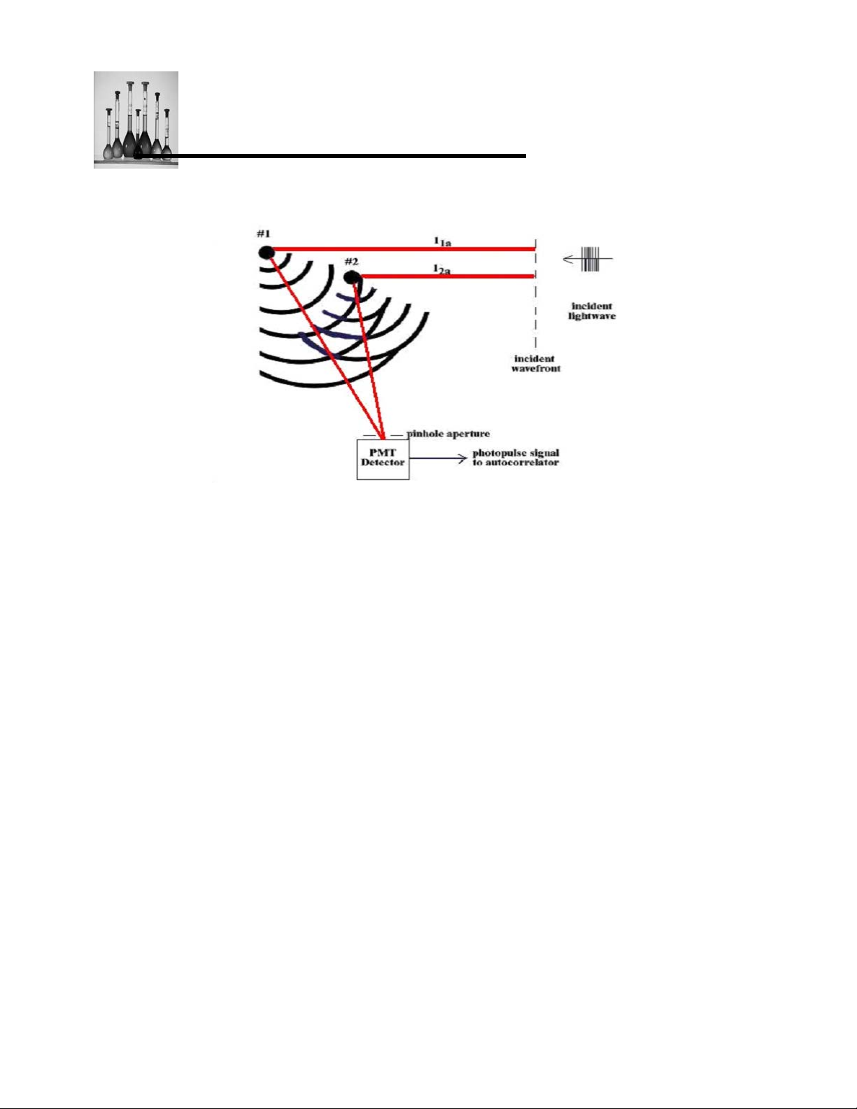
are only two particles in suspension, shown in Figure 2.

The net intensity at the detector (located far from the scattering cell, with a pinhole aperture) is a
result of the superposition of only two scattered waves. In Figure 2 we have defined the two
optical path lengths, L
distance corrected by the index of refraction, but for simplicity we assume an index of 1.0 and
show L

and L2 to be simple distances in Figure 2.) When the positions of the two particles are

1

such that the difference
multiple of the laser wavelength λ, then the two scattered waves will arrive in phase
detector. This is called total "constructive" interference and produces the largest possible
intensity at the detector.

= l1a + l1b and L2 = l2a + l2b. (More precisely, the optical path length is the

1

in optical path lengths, ΔL = L1 - L2 becomes equal to an integral

at the

Nicomp 380 Manual

PSS-380Nicomp-030806

06/06

Page 2 -3

DDLLSS TThheeoorryy

Figure 2: Simplified scattering model: two diffusing particles

At the other extreme, it is possible for the two particles to find themselves at positions such that

ΔL equals an odd number of half wavelengths, λ/2. In this case the two scattered waves arrive

at the detector totally out of phase with each other. This is total "destructive" interference,
resulting in zero net intensity. Over time, diffusion of the particles will cause the net intensity at
the detector to fluctuate in random fashion -- like a typical "noise" signal -- between these two
extreme values. A representative total intensity signal is shown in Figure 3. The intensity varies
between the maximum value and the minimum value (zero) when the optical path length
difference changes (i.e. increases or decreases) by λ/2.

Nicomp 380 Manual
PSS-380Nicomp-030806
06/06
Page 2 - 4

DDLLSS TThheeoorryy

Figure 3: Typical intensity vs time for two diffusing particles

The key physical concept that underlies the DLS particle sizing measurement is the fact that the

time scale of the fluctuations shown in Figure 3 depends on the size of the particles. For

simplicity at this point in the discussion, we assume the particles to be uniform in size, with a
single, well-defined diffusion coefficient. Small particles will "jitter" about in solution relatively
rapidly, resulting in a rapidly fluctuating intensity signal; by contrast, larger ones will diffuse
more slowly, resulting in a more slowly varying intensity.

At this point we make the simplifying assumption that the temperature of the particle suspension
is held constant. We shall see that the temperature plays as important a role as the particle
size in determining the diffusivity and, hence, the time scale of the resulting intensity
fluctuations. In any real situation of interest, of course, there are many more than two particles
in suspension which contribute to the scattered intensity signal. However, the principle of
interference remains the same. The resulting signal will be observed to fluctuate average level,
which is proportional to the number of particles illuminated/detected volume and their individual
scattering power -- Equations 1a and 1b. The time scale of the fluctuations depends on the
particle diffusivity, and hence on the particle size. This is illustrated in Figures 4a,b and c for
"small", "medium" and "large" size particles (using the same time scale on all three horizontal

axes). Again, it must be stressed that the fluctuations in the net scattered intensity are not

caused by the addition or subtraction of particles in the illuminated/detected volume. Rather,
they are the result of the variations in position of an essentially fixed number of particles within
the scattering volume.

Nicomp 380 Manual

PSS-380Nicomp-030806

06/06

Page 2 -5

DDLLSS TThheeoorryy

Figure 4 a,b,c: Representative intensity vs time for "small"(a), "medium"(b) and "large"(c) size
particles

Nicomp 380 Manual
PSS-380Nicomp-030806
06/06
Page 2 - 6

DDLLSS TThheeoorryy

Obtaining particle size from the diffusion coefficient

The goal of the DLS technique is to determine the diffusion coefficient D of the particles
(assumed uniform here) from the "raw" data -- i.e. the fluctuating light scattering signal, as
represented in Figure 4a,b,c. From D we can easily calculate the particle radius R. using the
well-known Stokes-Einstein relation,

D= kT/6πηR (2)

where k is Boltzmann's constant (1.38 X 10
the shear viscosity of the solvent (e.g. η = 1.002 X 10
that the rate at which the particles jitter about in the suspension, as measured by D, is inversely
related to the particle radius R.

From Equation 2 we see that, in general, the diffusion coefficient D of particles of a given size
increases with increasing temperature T. This is due primarily to the T-dependence of the
solvent viscosity η. (The fact that T is the numerator in Equation 2 is less small, in percentage,
when expressed in deg. Kelvin.) For example, η for pure water falls to 0.890 X 10

o

25

C -- i.e. more than a 10% change from the value at 20oC. Clearly, the less viscous the

solvent, the more rapid will be the random-walk diffusion of the particles and the faster the

resulting intensity fluctuations. Hence, changes in T are completely indistinguishable from

changes in particle radius R. as they affect D. For this reason, the sample temperature MUST
be constant (and accurately known) in order to obtain a meaningful measurement of D and,
hence, of R using Equation 2.

A cursory examination of the three fluctuating scattering signals in Figure 4a,b,c suggests that
extraction of the diffusion coefficient from the "noise" is not a straightforward matter. Signal (b)
clearly fluctuates faster than does (c), but is slower than (a); hence, its particle size must lie
between the values associated with (a) and (c). However, obtaining quantitative information
from these kinds of scattering signals is another matter altogether. What comes to our rescue is

the mathematical operation known as autocorrelation.

-16

erg K-1), T the temperature (oK, = oC + 273) and η

-2

poise for water at 20oC). Thus, we see

-2

poise at

Nicomp 380 Manual

PSS-380Nicomp-030806

06/06

Page 2 -7

DDLLSS TThheeoorryy

Autocorrelation function: definition and motivation

Let us consider the autocorrelation function of the net scattered light intensity I
fluctuates in time as shown in Figures 4a, b, and c. The autocorrelation function, which we
denote by C(t′) is used to study the correlation, or similarity, between the value of I
time, t, and the value of I

at a given time, t and the value of Is at an earlier time, t-t'. This

s

comparison is then made for many different values of t in order to obtain a good statistical
average for C(t') -- i.e. averaged over many "wiggles" of the fluctuating intensity I
evaluated according to,

C(t') = < I

(t) * Is(t-t')> (3)

s

The bracket symbols < > are shorthand for a summation over many values of t. That is, one
calculates a running sum of many products I

(t) * Is (t-t'), all having the same separation in time,

s

t', for many different values of t.

The ability of C(t') to extract useful information from the fluctuating scattering intensity I
best be understood by considering a portion of a typical signal I
arbitrarily choose a particular time t and record the value of I
consider a very small value of t', equal to t
I

(t-t1'). Because t1′ is presumed to be small, Is(t-t1') must be very similar to Is(t). The reason for

s

', and evaluate Is at this slightly earlier time, t-t1' --

1

(t), shown in Figure 5. We

s

at that time -- Is(t). We next

s

this, of course, is that the particles have not been able to change their positions significantly (i.e.
compared to λ) under diffusion in the (presumed) short time interval t
shown to be slightly larger than I

(t).

s

'. In Figure 5 Is(t-t1') is

1

(t), which

s

at a given

s

. C(t') is

s

(t) can

s

Figure 5: Computation of autocorrelation function C(t')

Nicomp 380 Manual
PSS-380Nicomp-030806
06/06
Page 2 - 8

DDLLSS TThheeoorryy

However, if t had been chosen differently in Figure 5, the order of the two values might have
been reversed. In any case, what matters is that the two intensity values that become multiplied
in Equation 3 are nearly the same. They are said to be highly correlated. Clearly, the choice of t
is irrelevant -- for any value of t, I
for a sufficiently small choice of t'.

Next, let us consider a larger value for t', equal to t

been chosen to be large enough relative to the time scale of the fluctuating signal that the two

sampled values of I

-- Is(t) and Is(t-t2') -- are now somewhat different. In this case, the two

s

sampled intensities are less well correlated. However, there still remains some relationship
between these two intensities. If t has been chosen so that I
intensity, then I

(t-t2') will still be a relatively low value. Similarly, if Is(t) lies near a maximum,

s

then it is apparent from Figure 5 that Is(t-t
not near a minimum), given the fact that t
characteristic time scale of the intensity signal shown in Figure 5.

Finally, we consider a very large time interval, t
large that I

has undergone two large fluctuations between the two sampling times, t and t-t3'. It

s

is clear, here, that the two sampled intensities will in general be almost completely uncorrelated

for such a large choice of t

'. The two values could easily be both high, both low, one high and

3

the other low, or any other intermediate possibility.

We have carried out these examples assuming a single choice for time t and three different
values of t'. In order to obtain a meaningful value for the autocorrelation function for a particular

choice of t' -- C(t') -- one must obtain many products I

for each value of t'. Only in this way will one average the value of C(t') over sufficiently many
"bumps" and "wiggles" in the fluctuating signal I
autocorrelation function. Then, one must repeat this process for sufficiently many values of t' so
as to obtain a well-defined, smooth representation of C(t') as a function of t'.

It is useful to have an idea at this point of the kinds of numbers that are involved when we use
the word "many". For a typical particle size measurement of duration 5 minutes on 0.2 micron

(200 nm) particles, the DLS Module performs approximately 15 million multiplications in order to
obtain C(t') for one value of t' (e.g. t' = 20 microseconds for "channel" #1). The instrument

makes 64 such sets of calculations simultaneously in order to obtain C(t') for 64 different values
of t'.

The essential point about the autocorrelation function is that it serves as a useful probe of the
characteristic lifetime, or duration, of the fluctuations in I
two sampled intensities exceeds the average width of a major "bump", or fluctuation, in I
two sampled intensity values will cease, on average, to be correlated. At this point, the value of
C(t') will have fallen substantially.

(t) and Is(t-t') must be highly correlated (i.e. nearly the same)

s

', as shown in Figure 5. In this case, t2' has

2

(t) is near a minimum in the

s

') must also be at a relatively high value (or certainly

2

' is not a very large time interval relative to the

2

', as seen in Figure 5. Here, we see that t3' is so

3

(t) * Is(t-t') using many different values of t,

s

to obtain a statistically meaningful value of the

s

(t). That is, once the interval t' between

s

(t), the

s

Nicomp 380 Manual

PSS-380Nicomp-030806

06/06

Page 2 -9

DDLLSS TThheeoorryy

What can we say about the shape of C(t') as a function of the sampling separation t'? Without
knowing anything about the physics of diffusion and its effect on I
something useful about C(t') in two limiting (extreme) cases: t' Æ0 and t'Æ:. In the limit in which
t' approaches zero, the two sampled intensities are essentially identical, because there is no
time for the particles to rearrange their positions. Hence,

C(O) = <I

2

(t)> (4)

s

That is, the value of C(t') for t'Æ0 is simply the sum over many values of t of the square
scattering intensity.

In the opposite limit, in which the sampling interval t' becomes very large (approaching infinity),
we have already seen (Figure 5) that there should be no correlation between the pair of
sampled intensities. Hence, Equation 3 reduces to the square of the average scattering
intensity, I

(t) -- i.e. the normalized sum of Is(t) values, taken over many values of t:

s

C(∞) = <I

(t)>2 (5)

s

It is known, and easily demonstrated, that for any fluctuating quantity, the average of the

squares of that quantity is always larger than the square of the average:

<I

2

(t)> > <Is(t)>2 (6)

s

The quantity on the right hand side of Equation 6 is the lowest value possible for the correlation
function; all other values of C(t') for finite values of t' must, in principle, be larger than the square
of the average of the I

values, because of the existence of correlations. This is referred to as

s

the baseline of the autocorrelation function. In practice, it can be effectively determined by

evaluating Equation 3 using a sufficiently large value for t'.

Hence, we can say with certainty that the function C(t') for our situation of diffusing particles
must fall from the value <I

2

(t)> at t'=0, to the baseline value, <Is(t)>2 at very large t'. The

s

problem remains -- what is the shape of C(t') between these two extreme values?

(t), we can nevertheless say

s

of the

Nicomp 380 Manual
PSS-380Nicomp-030806
06/06
Page 2 - 10

DDLLSS TThheeoorryy

Ideal case: uniform particle size

It turns out that for random diffusion of non-interacting particles, the autocorrelation function
C(t') of the fluctuating scattered light intensity I
t', as shown symbolically in Figure 6. This is described by the expression,

C(t') = A exp(-t'/τ) + B (7)

where A = <I
and B = <Is(t)>

2

(t)> - <Is(t)>

s

2

(t) is an exponentially decaying function of time

s

2

Figure 6:Autocorrelation function C(t') for diffusion of uniform particles: exponential
decay

Variable τ is the characteristic decay time constant of the exponential function; τ characterizes
quantitatively the speed with which the autocorrelation function C(t') decays toward the long-t'
limiting value (baseline B). In effect, the value of τ describes the characteristic lifetime, or
duration, of a major "bump", or fluctuation, in the scattered intensity I
particles, the slower the diffusivity and resulting fluctuations in I

s

. Hence, the larger the

s

' and the longer the decay time

constant τ.

As you might have predicted by now, we are able to obtain the diffusion coefficient D of the
particles from the decay constant τ; the precise relation is,

Nicomp 380 Manual

PSS-380Nicomp-030806

06/06

Page 2 -11

DDLLSS TThheeoorryy

1/τ = 2DK

2

(8a)
or
D = (1/2K

)(1/τ) (8b)

2

Here, the quantity K is called the "scattering wave vector". It is a constant that depends on the
laser wavelength λ in the solvent and the angle θ at which scattered light is intercepted by the
PMT detector. (θ = 90

o

for the DLS MODULE) In effect, K acts as an absolute calibration
constant, which relates the time scale of the diffusion process to the distance scale set by the
laser wavelength (making interference possible). Constant K is given by

K = (4πn/λ) sin θ/2 (9)

where n is the index of refraction of the solvent (e.g. 1.33 for water). In the case of the DLS
Module, with θ = 90

o

and λ = 632.8 nm, K equals 1.868 X 105 cm-l.

The rationale for particle sizing using the method of DLS should now be clear. We detect
scattered light (at a fixed angle) produced by an ensemble of particles suspended in a solvent.
The intensity fluctuates in time due to diffusion of the particles; there is a well defined
characteristic lifetime of the fluctuations, which is inversely proportional to the particle diffusivity.
We compute the autocorrelation function of the fluctuating intensity, obtaining a decaying
exponential curve in time. From the decay time constant τ, we obtain the particle diffusivity D.
Using the Stokes-Einstein relation (Equation 2), we finally compute the particle radius R
(assuming a sphere).

Photon counting and digital autocorrelation functions

We now consider the practical application of the theory discussed above in an actual DLS
particle sizing instrument. The first step is computation of the autocorrelation function C(t') from
the scattered light intensity I
fundamental operation of multiplication is most easily accomplished if both I
expressed as digital quantities. Fortunately, it turns out that this is already the case! In our
discussion thus far, we have represented I
magnitude as a function of time -- e.g. Figure 3 and 4a, b and c. However, in reality this is not
correct. The scattering signal I
produced by the PMT detector (Figure 1). That is, the particle suspension is sufficiently dilute
that the average scattering intensity at the PMT photocathode is extremely low, resulting in a
"photocurrent" which consists of discrete pulses (separated by zero baseline current),
corresponding to individual photons which comprise the weak scattering signal. Hence, the
DLS instrument is said to operate in the "photon counting" regime.

(t)' as prescribed in Equation 3. It should be apparent that the

s

(t) and Is(t-t') are

s

as an analog signal which varies continuously in

s

actually consists of a series of individual "photopulses"

s

Nicomp 380 Manual
PSS-380Nicomp-030806
06/06
Page 2 - 12

DDLLSS TThheeoorryy

If Is consists of a train of discrete pulses, rather than an analog signal, what is the quantitative
meaning of the "intensity" I
of photopulses per unit of time; the larger the number of pulses occurring in that time unit, the
larger the intensity. For example, in typical operation the DLS Module might show a photopulse
rate of, say, 300 kHz. This value is updated every one second and represents the number of
photopulses detected in the proceeding one-second interval. The sequence of values might
resemble the series 302, 297, 299, 304, 296, etc. We would therefore say that the average
"intensity" is approximately 300,000 -- meaning, pulses per one-second interval. However, it
would be equally valid to express the average intensity as 150,000 -- meaning per 0.5-second
interval; or as 30,000 -meaning per 0.1-second interval. That is, any
any other, for the purpose of defining the average value of the scattered intensity, depending on
the length of time which one wishes to use to define that average value.

Earlier we saw that it is typically necessary to sample the value of I

choose small values of t' between sampled pairs) in order to obtain an accurate autocorrelation

function, which is sensitive to rapid changes in I
this reason, it is therefore necessary to define I
small unit of time. In this way, the measurement of I
and approaches being an instantaneous value. For example, when 100 nm (0.1 micron)
particles are measured by the DLS Module, the sampling of I
every 10 microseconds. In this case, therefore, I
photopulses which occur during a given 10 microsecond interval. This short a time interval, or
smallest increment in t', is needed to compute the relatively rapid decay of C(t') versus t' which
occurs for these rapidly diffusing small particles. Of course, for smaller particles an even smaller
unit time interval would be needed to define I

Two observations should immediately be evident. First, given such small time intervals used to
define I

(t), the resulting number of pulses must be very small. Consider our example of a

s

typical average photopulse rate of 300,000 per second; this corresponds to an average
instantaneous intensity of 3 pulses per 10 microseconds. Second, we should expect this
number to change greatly from one time interval to the next, given such a small average value.
If the instantaneous photon rate were to follow Poisson statistics, we would expect the rms
standard deviation of the number of pulses per time interval to equal N
average number. For our example above, this gives a standard deviation of 1.7. Hence, from
purely a statistical point of view we expect the "intensity" I
vary from 0 to 5 photopulses with occasionally a 6, 7 or larger), independent of the effects of
diffusion. This is simply a consequence of our having chosen a very short time interval relative
to the average photopulse rate. When diffusion is added to the process, the resulting
fluctuations in I

(t) become even more pronounced.

s

The resulting integer numbers of photopulses per small time interval are, of course, the values
of I

(t) and Is(t-t') in Equation 3 which become multiplied together digitally to compute the values

s

of C(t'). A representative sequence of photopulses is shown in Figure 7. We have subdivided
the time base, t, into intervals of equal width Δt', equal to the "channel width" of the

at time t? Clearly, the intensity must be represented by the number

s

unit of time is as valid as

(t) very frequently (i.e. to

s

, caused by rapid diffusion of the particles. For

s

, in terms of the photopulse rate using a very

s

can be made as frequently as necessary

s

(t) is performed approximately

s

(t) is arbitrarily defined to be the number of

s

(t).

s

1/2

, where N is the

per 10 microsecond time interval to

s

Nicomp 380 Manual

PSS-380Nicomp-030806

06/06

Page 2 -13

DDLLSS TThheeoorryy

autocorrelator. Here, the instantaneous intensity Is(t) is defined as the number of pulses in the
interval Δt' which lies closest to time t. Over each interval we have recorded the instantaneous
"intensity" for that interval -- simply the number of photopulses produced by the PMT detector.
(Technically, the pulses which comprise the PMT photocurrent vary substantially in height, as
well as rate of Occurrence, owing to the statistical nature of the secondary-electron
multiplication mechanism in the PMT.

Figure 7: A typical photopulse sequence representing I
time width, t'

However, a discriminator with a low reference level is used to convert this signal to a
train of pulses of uniform height, suitable for manipulation by standard integrated logic circuits in
the autocorrelator.)

The procedure for computing the digital representation of C(t') should now be conceptually
clear. The train of photopulses from the PMT detector is divided into intervals of equal time, or
channel width, Δt'. Running sums of the products I
values of t' -- 64 in the case of the DLS Module. The separation times t' are "quantized" in
multiples of Δt': Δt', 2Δt', 3Δt',...64 Δt'. In addition, a long-delay baseline value is obtained:
t' = (64 + 1024) Δt'.

(t) * Is(t-t') are then produced for many

s

(t) divided into intervals of equal

s

Nicomp 380 Manual
PSS-380Nicomp-030806
06/06
Page 2 - 14

DDLLSS TThheeoorryy

Using the photopulse sequence shown in Figure 7, we now show how to compute the values of
C(t') for the first few "channels" in t':

t' = Δt': C(t') = 2*3 + 3*1 + 1*4 + 4*2 + 2*0 + 0*3 + 3*1 + ...

t' = 2Δt': C(t') = 2*1 + 3*4 + 1*2 + 4*0 + 2*3 + 0*1 + ...

t' = 3Δt': C(t') = 2*4 + 3*2 + l*0 + 4*3 + 2*1 + ...

t' = 4Δt': C(t') = 2*2 + 3*0 + 1*3 + 4*1 + ...

etc.

In the following section we shall generalize our discussion to include "polydisperse" systems -­those that contain a mixture of particle sizes. We shall discuss in some detail the methods by
which the DLS Module is able to deal effectively with these more complex systems. These are
the so-called "algorithms" for analysis of the autocorrelation function, which yield estimates of
the true particle size distribution. The next section will be heavily weighted toward results -- i.e.
actual pictures of screen displays and printouts -- and less concerned with theoretical details.
Hence, if you have survived the proceeding discussion and equations, you have our
congratulations (!) and assurance that you should experience clear sailing in the section ahead.
In any case, you are STRONGLY URGED to read Section C carefully. It should help you
appreciate the power of the DLS technique when applied to "difficult" particle size distributions,
like those that are frequently encountered.

Nicomp 380 Manual

PSS-380Nicomp-030806

06/06

Page 2 -15

DDLLSS TThheeoorryy

THE SIMPLEST APPROACH TO SIZE DISTRIBUTIONS: GAUSSIAN ANALYSIS

Uniform particle size- trivial analysis

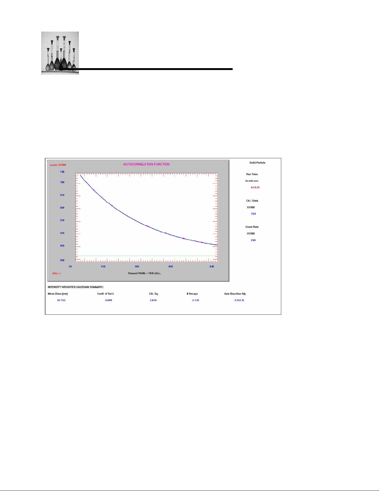
In Figure 8a we see a video display of the 64-channel autocorrelation function obtained using
DLS for a 90 nm (0.090 micron) polystyrene latex particle size standard.

Figure 8a: Autocorrelation function for 91-nm latex standard.

This particular sample has been chosen for this example because of its high uniformity of

particle size -- i.e. it is nearly “monodisperse”.

Nicomp 380 Manual
PSS-380Nicomp-030806
06/06
Page 2 - 16

DDLLSS TThheeoorryy

Figure 8b shows a printout of the block of raw autocorrelation channel data corresponding to
Figure 8a.

Nicomp 380 Manual

PSS-380Nicomp-030806

06/06

Page 2 -17

DDLLSS TThheeoorryy

Figure 8b: Block of raw data corresponding to Figure 8a

The channel width, Δt’, for this particular run was 10 μsec (microseconds). It is instructive to

verify that this autocorrelation function, C(t’), closely approximates the ideal result of a single
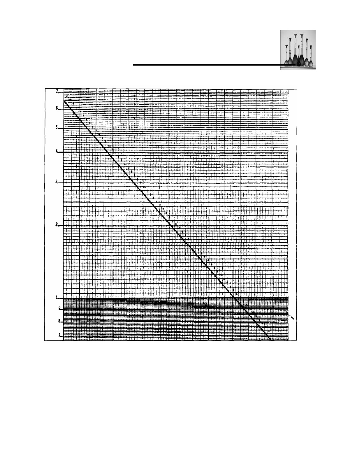
decaying exponential function. To do this we plot C(t’)-B (B=baseline) versus t′ (i.e. channel

number) on semi-logarithmic graph paper. A perfectly straight line of negative slope should

result, according to our previous discussion (Equation 7). This is shown in Figure 8c. The solid

straight line has been drawn by eye to best approximate the slope established by the data

points, log

latter to be clearly seen.

( C(t’)-B). We have deliberately displaced the line below the points to permit the

e

Nicomp 380 Manual
PSS-380Nicomp-030806
06/06
Page 2 - 18

DDLLSS TThheeoorryy

Figure 8c: Loge( C(t’)-B ) vs t’ for data of Figures 8a and 8b

Nicomp 380 Manual

PSS-380Nicomp-030806

06/06

Page 2 -19

DDLLSS TThheeoorryy

Using Equations 7-9 we can now calculate the particle diameter predicted by the semilog

behavior shown in Figure 8c. From Equation 7, we have

log

( C(t’)-B ) = 1ogeA – t’/τ (l0a)

e

= log

A - 2DK2t’ (l0b)

e

The slope in Figure 8c is -2DK

-8

D = 5.08 X 10
R =4.57 X 10

cm2/s. From Equation 9, with T =230C and η = 0.932 X 10-2 poise, we obtain

-6

cm, or 45.7 nm (457 Angstroms). This diameter of 91.4 nm agrees very well with

the nominal size of this particular Dow polystyrene latex standard. (Its mean volume-averaged

diameter is generally agreed to lie in the range 89-90 nary.)

Unfortunately, the simple, straightforward analysis just discussed has only limited usefulness.

As must be obvious to all but the most casual observers, most samples of practical interest

differ appreciably from the uniform, “monodisperse” case discussed in the previous section.

“Real” samples usually contain a range of sizes, often of substantial width, and are said to be

“polydisperse”. Such a particle size distribution might be conceptually simple, consisting of a

smooth, single-peak (“unimodal”) population of well defined mean diameter and width. Or, the

distribution might be qualitatively more complex, resembling two discrete peaks (a “bimodal”

distribution), or an even more complicated shape.

We shall see that two very different mathematical procedures, or “algorithms”, have been

developed to analyze the autocorrelation “raw data”, C(t’), depending on the nature of the

underlying particle size distribution. The software automatically selects the more appropriate of

the two analysis procedures and provides the user with a running measure of the accuracy, or

“goodness of fit”, of the computed distribution resulting from the particular analysis chosen.

Nevertheless, we feel it essential to gain an appreciation of the rationale behind each of the

analysis methods and to become comfortable with some typical results obtained for actual

particle systems. The latter can be studied in a controlled, accurate way using polystyrene

latexes, oil-in-water emulsions and other well-characterized materials.

2

, where K2 = 3.489 X 1010cm- 2, we obtain the particle diffusivity,

Nicomp 380 Manual
PSS-380Nicomp-030806
06/06
Page 2 - 20

DDLLSS TThheeoorryy

Broad unimodal distribution Gaussian Analysis

Following the discussion in the previous section, it is now obvious that a mixture of particle sizes

must give rise to an autocorrelation function C(t’) which decaying exponential function is no
longer a simple i.e. having a single, well-defined decay time constant τ, as shown in Figure 8c.

The existence of more than one rate of diffusion must necessarily give rise to a mixture of
decaying exponential functions, each of which has a different time decay constant τ

corresponding to a particular diffusivity D and, hence, of particle radius R

. The challenge which

i

we face is to develop fast and efficient mathematical methods of analysis, whereby we can

“deconvolve” C(t’) and thereby extract the distribution of D values (and hence of particle

diameters) from the detailed shape of C(t’). The “magic” behind the DLS Module has to do with

its ability to obtain, accurately and consistently, the most useful information relating to the

distribution of particle sizes in solution. To do this, the 380 must analyze precisely the deviations

of autocorrelation function C(t’) from single-exponential behavior. As we shall discover below,

these deviations are often surprisingly slight and subtle, given the large range of complicated

distributions which are encountered.

The simplest kind of complexity in the particle size distribution that we can introduce is a

smooth, gaussian-like population of sizes, having a well-defined mean diameter and half width.

Such an idealized distribution shape is often obtained for emulsions, prepared by a variety of

processes, sonication, homogenization and Microfluidization

TM

. Typically, some type of oil and

water are caused to be mixed together with the aid of a dispersing agent (e.g. a non-ionic

surfactant) to form a single, microscopically homogeneous phase. The result: tiny droplets of

one component (e.g. the oil) suspended in the other component, or “phase” (e.g. water). The

mean size and width of the resulting droplet distribution are usually sensitive functions of the

stoichiometry of the starting compounds and the duration and detailed nature of the preparation

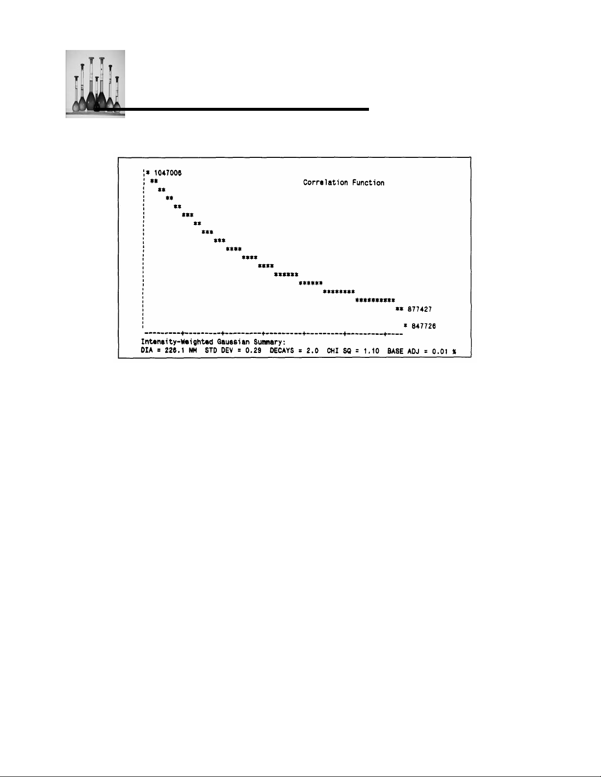
technique employed. In Figure 9a we show the autocorrelation function for a fat emulsion, used

for intravenous (“IV”) feeding. The channel width used here was 21 usec.

i

Nicomp 380 Manual

PSS-380Nicomp-030806

06/06

Page 2 -21

DDLLSS TThheeoorryy

Figure 9a: Autocorrelation function for an IV fat emulsion.

Let us make a visual comparison between Figure 9a and 8a, obtained for the narrow 91 nm

latex standard. The shapes of the two decaying curves appear to be quite similar, which is

somewhat surprising given the differences between the two samples. Qualitatively, we conclude

that the average, or characteristic, particle diameter associated with Figure 9a must be roughly

twice that associated with Figure 8a. The reason: both curves possess about the same number

of “decays” in falling to the 64th channel, and the channel width for the latter sample is twice

that of the former.

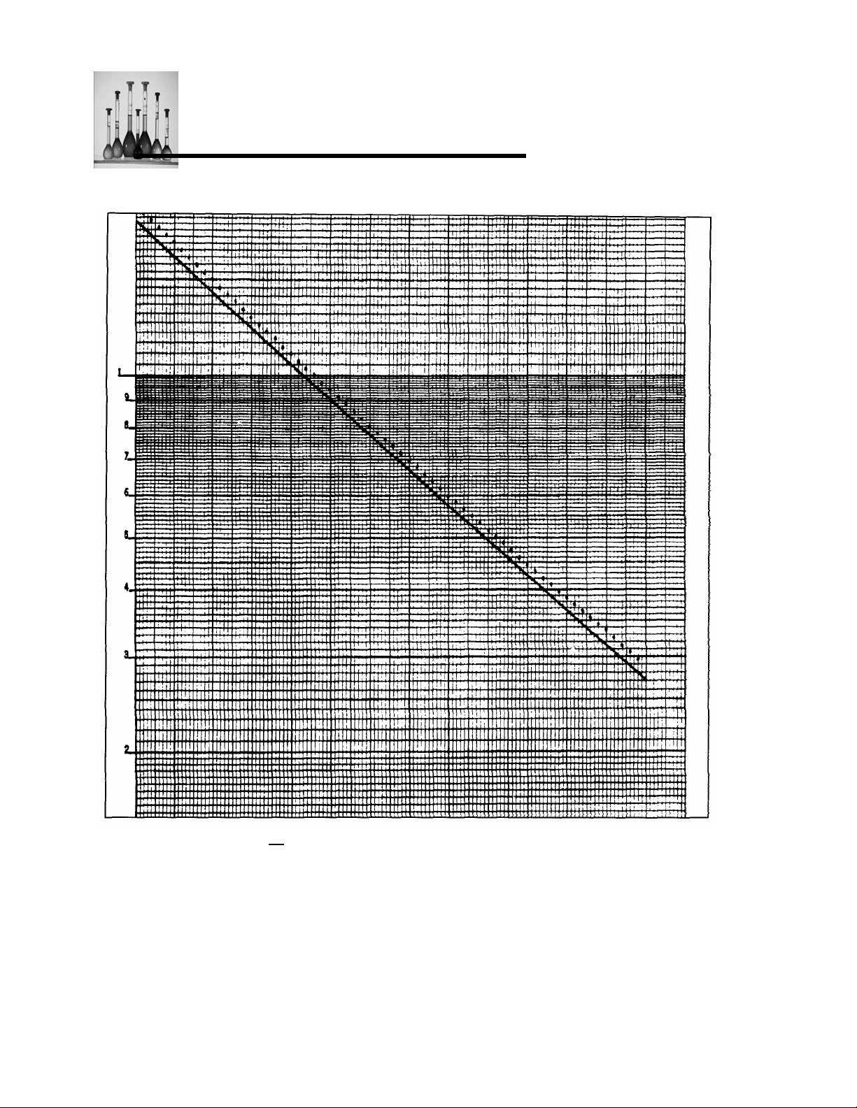
We can acquire a better appreciation of the subtlety of the analysis task which faces us by

looking at the reduced data, C(t’)-B, on a semilog plot in Figure 9b and comparing this with the

previous reduced data for the narrow 91-nm latex standard, Figure 8c. Indeed, we must look

closely to find any qualitative difference between the two plots! However, on closer examination

we see that the reduced data points in Figure 9b possess a slight curvature; a displaced straight

line has been drawn to enable this curvature to be seen. As we shall see in a moment, this fat

emulsion sample does indeed possess a substantial width, or range of sizes, in its particle size

distribution. Therefore, what may seem surprising (and, perhaps, intimidating) is how relatively

little deviation there is from the single-exponential behavior of C(t’) in Figure 9b, given the

apparently large qualitative difference in distribution shapes between the “sharp” latex standard

and the “broad” emulsion sample.

Nicomp 380 Manual
PSS-380Nicomp-030806
06/06
Page 2 - 22

DDLLSS TThheeoorryy

The example above illustrates the inherent difficulty which all DLS-based particle sizing

instruments face: what distinguishes the shape of one computed particle size distribution from

another is often a relatively subtle deviation of C(t’) from single exponential behavior. Hence, we

MUST learn to appreciate the importance of acquiring data of high statistical accuracy.

Nicomp 380 Manual

PSS-380Nicomp-030806

06/06

Page 2 -23

DDLLSS TThheeoorryy

Figure 9b: Log

This requirement is intimately related to the run time and the efficacy of sample preparation. Not

surprisingly, it turns out that there are NO ‘short cuts” to obtaining good raw data and, hence,

good analyses. Suffice to say, there is more than meets the eye in the successful extraction of

particle size distributions using the DLS technique! More evidence will unfold below, supporting

the claim that this can be a difficult business. Nonetheless, let us take courage and press on.

Nicomp 380 Manual
PSS-380Nicomp-030806
06/06
Page 2 - 24

( C(t’)-B) vs t’ for data of Figure 9a.

e

DDLLSS TThheeoorryy

What is needed, clearly, is a method for dealing with the “simple” kind of polydispersity in the

particle size distribution illustrated by the IV emulsion example above. The word “simple” is used

to emphasize the fact that we have gone from a sharp population, consisting of essentially one

size, to one which represents a smooth, not-too-wide range of sizes centered about some

average. In the case of a sharp distribution, it is a simple matter to obtain the “best” straight-line

fit to the logarithm of the reduced data, loge C(t’)-B) vs t’, using the well-known method of least

squares. One simply adjusts the slope and intercept of the straight line to minimize the sum of

the squares of the deviations, or errors, between the reduced data points and the values implied

by the “theory” -- i.e. by the straight line.

The needed generalization which can deal effectively with non-exponential behavior of C(t’)-B,

brought about by smooth, Gaussian-like distributions of particle diameters, is provided by the

methods of cumulants. This procedure, first introduced by Koppel, has been used extensively in

the past 15 years to obtain estimates of the particle size distribution from DLS. In fact, until only

5 or 6 years ago it was essentially the only practical method for obtaining such information. The

conceptual underpinning of the cumulants procedure is simplicity itself, as will be seen below.

Suppose we consider situations for which the plot of log

curvature, representing a modest deviation from straight-line behavior. The simplest

generalization of the straight-line fitting procedure is to find the quadratic function of C which lies

closest to the reduced data points (i.e. on a least-squares basis). The prescription for carrying

out a cumulants fit is, therefore, very simple, as summarized below:

1/2 log

( C(t’)-B ) ↔ a

e

+ a1(t’) + a2(t’)2 (11)

0

A quadratic function of C, which we’ve indicated by a

straight-line function, b

function -- in particular, a

+ b1(t’). All that remains is to relate the coefficients of the quadratic

0

and a2 -- to parameters that describe the corresponding particle size

1

distribution.

In the simple monodisperse case discussed earlier, we recall (Equations l0a and b) that

coefficient b

equals -DK2. Hence, the value of the slope (negative), divided by the constant K2,

1

yields the diffusion coefficient D of the (uniform) particles. It turns out in the more general case

of a quadratic fit that the distribution of diffusion coefficients D

Gaussian, or normal, shape. This is a bell-shaped distribution that requires only two parameters

for its full description (not including the peak magnitude, which is arbitrarily set equal to 100 for

Nicomp 380 Manual

( C(t’)-B ) has a relatively small

e

+ a1(t’) + a2(t’)2, now replaces the trivial

0

is approximately equal to a

i

PSS-380Nicomp-030806

Page 2 -25

06/06

DDLLSS TThheeoorryy

all of our relative particle size distributions). These are the mean diffusivity, D, and the half width
ΔD of diffusivity values. (Strictly speaking, the cumulants fit results in an approximately
Gaussian distribution of intensity-weighted diffusivities. This point will be discussed later.)

The connection between coefficients a
logarithm of the reduced data, and the parameters D and ΔD of the Gaussian distribution of

diffusivities, is given by
a

or, D = -a

and ΔD/D = 2a

Equation 13 gives the normalized standard deviation (or coefficient of variation) of the diffusivity
distribution -- i.e. standard deviation ΔD divided by the mean diffusivity D. Naturally, the width
parameter ΔD is related to coefficient a

data. For distributions that are very narrow -- nearly monodisperse -- we expect a

small, so that the quadratic function effectively reduces to being a straight line.

Ultimately one wishes to have the result expressed in terms of a distribution of particle radii R

(or diameters), rather than of diffusivities D. This is not a problem, of course, because the

Stokes-Einstein relation (Equation 2) shows that D is simply given by 1/R times a conversion

constant. Furthermore, for relatively small ranges of D a Gaussian distribution in 1/R translates

into a Gaussian shape in ln R. Hence, we arrive at approximately a log-normal shape for the

distribution of particle radii (or diameters). Using the Stokes-Einstein relation (Equation 2) and

Equations 12b and 13 we can therefore obtain the mean particle diameter, d = 2R, and the
standard deviation of the diameter distribution, 2 * ΔR. This latter parameter is also known as

the “coefficient of variation” and is equal to the square root of the “variance”; it is closely related

to the half width of the particle size distribution, which is approximately a log normal in shape.

In the DLS Module we refer to this cumulants method for “inverting” the autocorrelation function

as the Gaussian Analysis. It must be stressed that it is 2-parameter fit; that is, except for the
possibility of a change in the baseline, there are only two variables which affect the goodness of

fit of the quadratic function of C with respect to the reduced data, log

These are coefficients a

and a2. (Coefficient a0 has relatively little value in the analysis -- it is

1

related to the contents of channel #1 of C(t’), which increases with the total run time, all other

Nicomp 380 Manual
PSS-380Nicomp-030806
06/06
Page 2 - 26

and a2, obtained from the best quadratic fit to the

1

= -DK

1

2

2

2

/K

1

/(-a1) (13)

2

(12a)

(12b)

, which describes the extent of curvature in the reduced

to be very

2

(C(t’)-B) (Equation 11).

e

DDLLSS TThheeoorryy

variables being equal.)

The result of the Gaussian Analysis when applied to the autocorrelation data of Figs. IV-9a,b is

shown in Figure l0a.

Figure l0a: Intensity-weighted Gaussian Analysis corresponding to the data of
Figure 9a and b.

This is the summary under the decaying curve C(t’), which is updated approximately every 30

seconds on the video display. It carries the label “Intensity Weighting” because it represents the

immediate result of the cumulants calculation, before any specific type of particle weighting is

taken into consideration. That is, the underlying autocorrelation function C(t’) is constructed

from the original scattered intensity values as a function of time. Hence, the quadratic fit and the

corresponding Gaussian-like representation of the distribution of particle diffusivities (and,

ultimately, diameters) reflect the fact that the D contributions, or R contributions, are weighted

by their corresponding scattering intensities. Again, the peak shown in Figure l0a is

approximately a Gaussian shape with respect to the log diameter scale -- i.e., it is approximately

a log normal shape (provided the standard deviation is not excessive -- < 25%, or so, of the

mean value).

Nicomp 380 Manual

PSS-380Nicomp-030806

06/06

Page 2 -27

DDLLSS TThheeoorryy

There are 6 pieces of quantitative information contained in the summary display of the Gaussian

Analysis (Figure l0a):

Mean Diameter 226.1 nm
Standard Deviation 30%
Chi Squared 1.1
Baseline Adjust 0.01 %
Data 1047.0 K
Mean Diffusion 2.05 X 10

The value 30% for the standard deviation means that ΔR/R=0.30.

A critical piece of information contained in Figure l0a is the value of Chi Squared. Any value

close to (or below) 1.0 indicates an exceptionally good fit of the quadratic function to the

reduced data. Assuming that sufficient statistics have been collected in the autocorrelation

function to make the value of Chi Squared meaningful (which is NOT true early into a run), a low

value means that the Gaussian representation of the particle size distribution is a good

assumption -- i.e. that no other distribution shape can offer a “better” fit to the data, given the

limitations implied by Poisson statistics. Indeed, the test of a good Gaussian Analysis result is

whether Chi Squared remains small (i.e. below 2 or 3) over the course of time, as additional

intensity values are collected and incorporated into autocorrelation function C(t’). The DLS

Module makes this judgment automatically and will provide an appropriate warning message if

the value of Chi Squared exceeds 3, suggesting that the Gaussian Analysis result is

inappropriate.

The value for Baseline Adjust shown above, 0.01 %, is very close to the ideal value of zero,

indicating that almost no adjustment in the value of B was needed to obtain the lowest value of

Chi Squared. Hence, this particular sample contained a negligible concentration of large-particle

aggregates or other contaminants.

The value for Data, 1047 K, represents the contents of channel #1 of the autocorrelation

function, C(t’). Such a relatively large value, exceeding one million (=1000 K), usually indicates

a high degree of statistical accuracy in C(t’). At this point, the results of the Gaussian Analysis

should have become stable, with relatively little change with additional run time. In the example

summarized above, 1047 K was achieved in channel #1 after a run time of 14 mm 48 sec. The

relationship between the value of Data and the run time will in general depend on the average

-8

cm2/sec

Nicomp 380 Manual
PSS-380Nicomp-030806
06/06
Page 2 - 28

DDLLSS TThheeoorryy

scattered light intensity and the channel width Δt’.

Nicomp 380 Manual

PSS-380Nicomp-030806

06/06

Page 2 -29

DDLLSS TThheeoorryy

Effects of weighting in the Gaussian Analysis

The problem with an intensity-weighted particle size distribution is that it is generally not very

useful in the “real” world. Typically, one wishes to obtain a size distribution that is either

weighted by particle number (a trivial “weighting”) or by particle volume, or mass (i.e. weighted

by diameter cubed). The DLS Module uses the “rules” of light scattering (including corrections

for Mie scattering, when intraparticle interference effects become important, for diameters

greater than about 150 nm) in order to obtain number-weighted and volume-weighted diameter

distributions from the starting result, which is an intensity-weighted plot. Note: “Volume”

weighting and “mass” weighting are equivalent terms.

The volume-weighted and number-weighted video displays corresponding to the example

discussed above are shown in Figure l0b and l0c, respectively.

The three display plots, Figure l0a, b and c, reveal an important property that is generally

observed when using the Gaussian Analysis. That is, the value of the mean diameter can vary

significantly with the choice of weighting, depending on the width of the Gaussian-like

distribution. In general, the wider the distribution (i.e. the larger the percentage standard

deviation), the greater the differences in mean diameter for the various weightings. In the

present example we see that the mean diameter of the volume-weighted peak (209. 1 nm) is

shifted almost 10% below that of the intensity-weighted result (226.1 nm). The number-weighted

mean diameter is reduced even more dramatically, to 144.7 nm.

Nicomp 380 Manual
PSS-380Nicomp-030806
06/06
Page 2 - 30

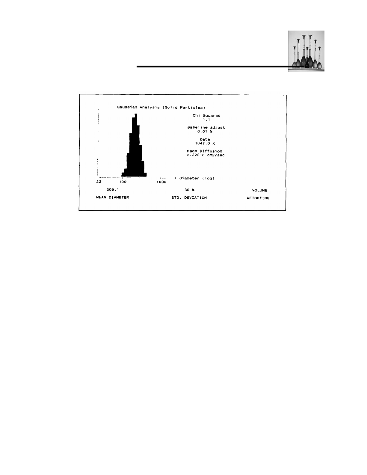
DDLLSS TThheeoorryy

Figure l0b: Volume-weighted Gaussian Analysis corresponding to Figure l0a
and data of Figures 9a and b.

This behavior can be easily understood qualitatively by reviewing the relationship between

particle size and scattering intensity, discussed in the previous section. For particle sizes

sufficiently small to permit neglect of the Mie “form factor” (arising from intraparticle interference

of individual scattered waves), we see from Equation lb that the contribution to C(t’) of a

particular decaying exponential, corresponding to a given diameter d

the factor N

individual volume, which is proportional to (d

)2, where Ni represents the number of particles having diameter di, and Vj is their

i(Vi

)3. Hence, each diameter “slice” of the starting

i

intensity-weighted distribution has associated with it this factor of N

, should be weighted by

i

2

)

i(Vi

Nicomp 380 Manual

PSS-380Nicomp-030806

06/06

Page 2 -31

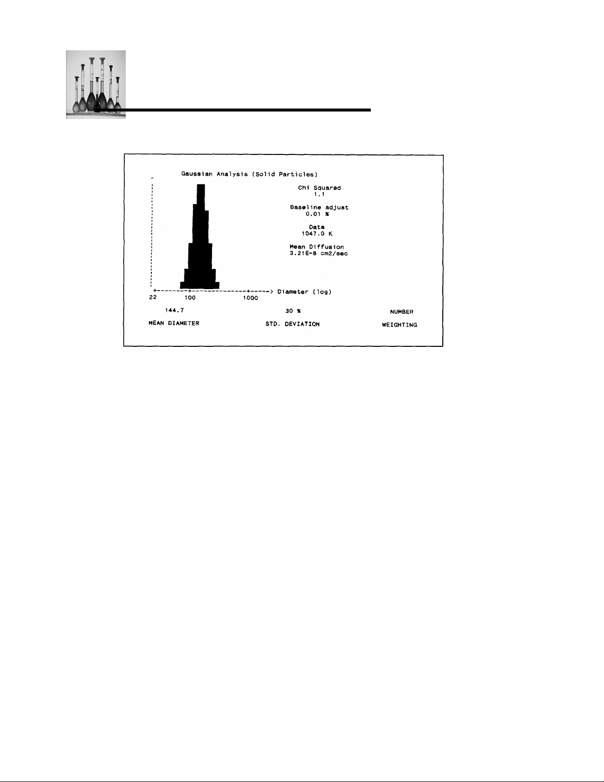
DDLLSS TThheeoorryy

Figure l0c: Number-weighted Gaussian Analysis corresponding to Figure l0a
and data of Figure 9a and b.

The constituent diameters of the volume-weighted distribution should each have the weighting

factor N

volume, or mass, for that diameter. These new factors are obtained from the previous intensity-

weighted factors by dividing each by V

shown above in Figure l0b. To obtain the number-weighted result, we perform one additional

division of the weighting factors by V

in Figure l0c above. In the case in which the intraparticle form factor cannot be ignored, it must

first be divided out of the original intensity-weighted factors.

The printouts that correspond to the three weightings discussed above are shown in Figure 11a,

b and c. The various distribution plots are labeled with two sets of numbers. The “REL” set is

normalized such that the peak value is always 100. The “PERCENT” set is normalized such that

the sum of all of the numbers equals 100%.

-- i.e. the number of particles having a particular diameter multiplied by the particle

iVi

, or (di)3. The resulting (approximate) distribution is

i

or (di)3, to obtain a final weighting factor of just Ni, shown

i

Nicomp 380 Manual
PSS-380Nicomp-030806
06/06
Page 2 - 32

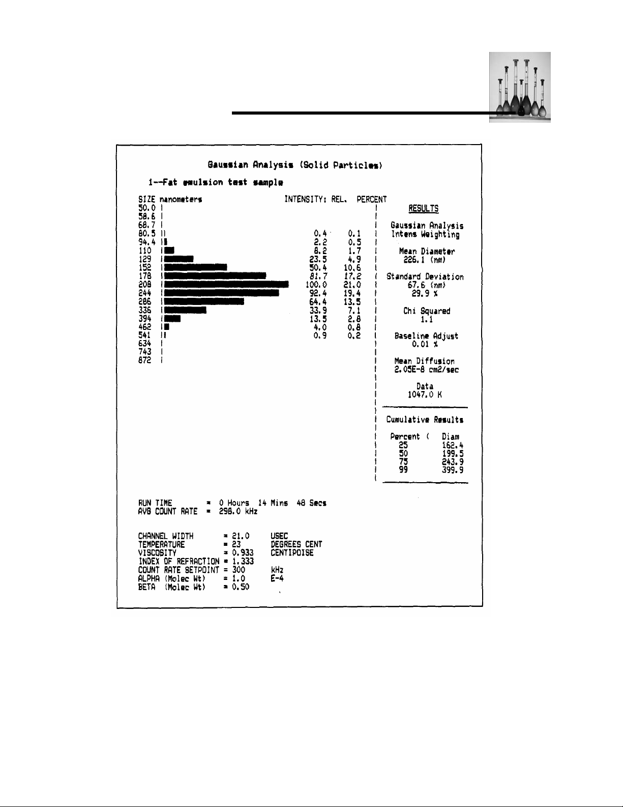
DDLLSS TThheeoorryy

Figure 11a: Printout of volume-weighted Gaussian Analysis result for fat emulsion

(See Figure l0a.)

Nicomp 380 Manual

PSS-380Nicomp-030806

06/06

Page 2 -33

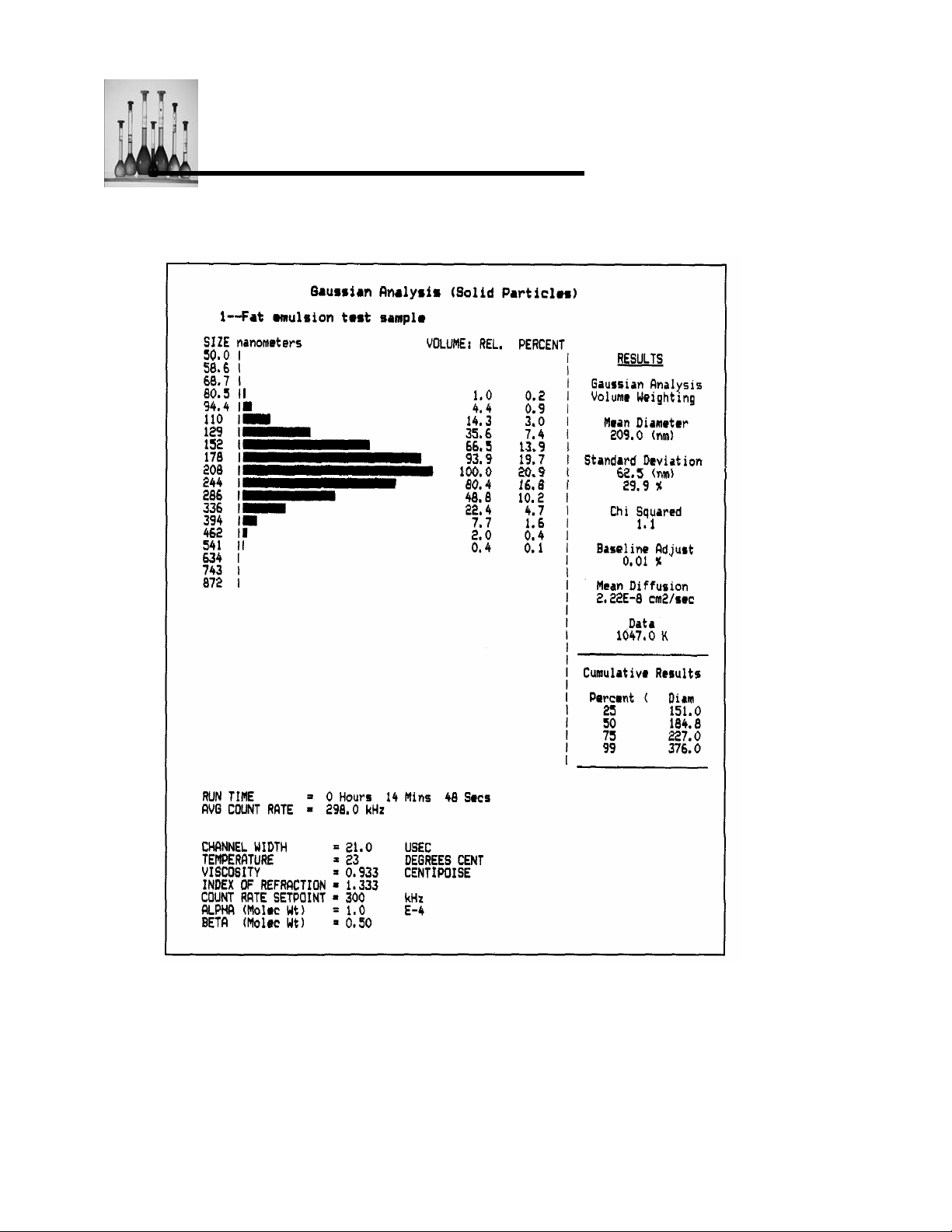
DDLLSS TThheeoorryy

Figure 11b: Printout of volume-weighted Gaussian Analysis result for fat emulsion.
(See Figure l0b.)

Nicomp 380 Manual
PSS-380Nicomp-030806
06/06
Page 2 - 34

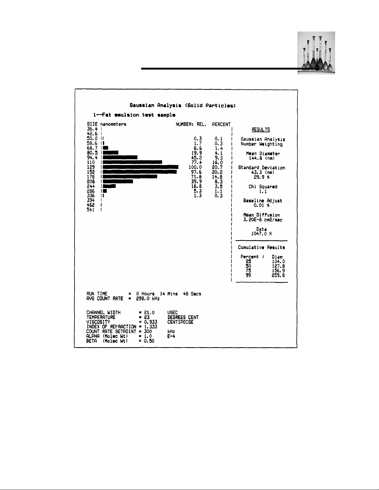
DDLLSS TThheeoorryy

Figure 11c: Printout of number-weighted Gaussian Analysis result for fat emulsion.
(See Figure l0c.)

Nicomp 380 Manual

PSS-380Nicomp-030806

06/06

Page 2 -35

DDLLSS TThheeoorryy

It MUST be re-emphasized that the distribution shapes shown in Figure l0a,b and c and Figure

11a,b,c are obtained from the tabulations for the Gaussian, or normal, curve found in standard

mathematical references. Their shape is an idealization and should NEVER be construed to

offer more detailed information than can legitimately be expected from this fitting procedure. The

peak shown in Figure 11b, for example, contains 13 discrete diameter slices, each evidently

possessing a well-defined height, or relative volume. In a way, this is misleading; this shape has

emerged from what is fundamentally just a 2-parameter fit (plus, possibly, a baseline adjust).

Hence, we should NEVER be lulled into believing the actual heights of each of the slices that

comprise the distribution curve. These values have originated from an idealized

mathematical table, not from a measurement procedure which counts particles one at a time.

Because the DLS technology is unable to measure particles individually, it yields only

smoothed, idealized estimates of the actual particle size distribution curves. Nevertheless, the

DLS Module will usually be found to be very sensitive to small changes in the shape of the

underlying particle size distribution.

Importance of acquiring data of sufficient accuracy

A central, repeated theme of this section will be the importance of acquiring autocorrelation data

of high statistical accuracy. If this is achieved, the resulting computed particle size distributions

will be found to be stable in time. As we shall see, the level of statistical accuracy required for a

reliable analysis depends greatly on the analysis method chosen. Because the Gaussian

Analysis is only a 2-parameter fit (with the possible addition of a baseline adjustment), it will

settle to a reliable result relatively quickly -- certainly faster than the NJCOMP Distribution

Analysis (discussed in the next section). This simply reflects the fact that the best quadratic fit to

the reduced autocorrelation data is relatively insensitive to small variations in individual data

points, given a total of 64 points for each fit. A good illustration of the typical settling time of the

Gaussian Analysis is provided by a tabulation of the results obtained for the IV fat emulsion

discussed above. A new computed distribution was obtained approximately every 45 seconds,

whenever a fresh set of analysis results was displayed on the video terminal; a summary of

these results is shown below in Table 1.

Nicomp 380 Manual
PSS-380Nicomp-030806
06/06
Page 2 - 36

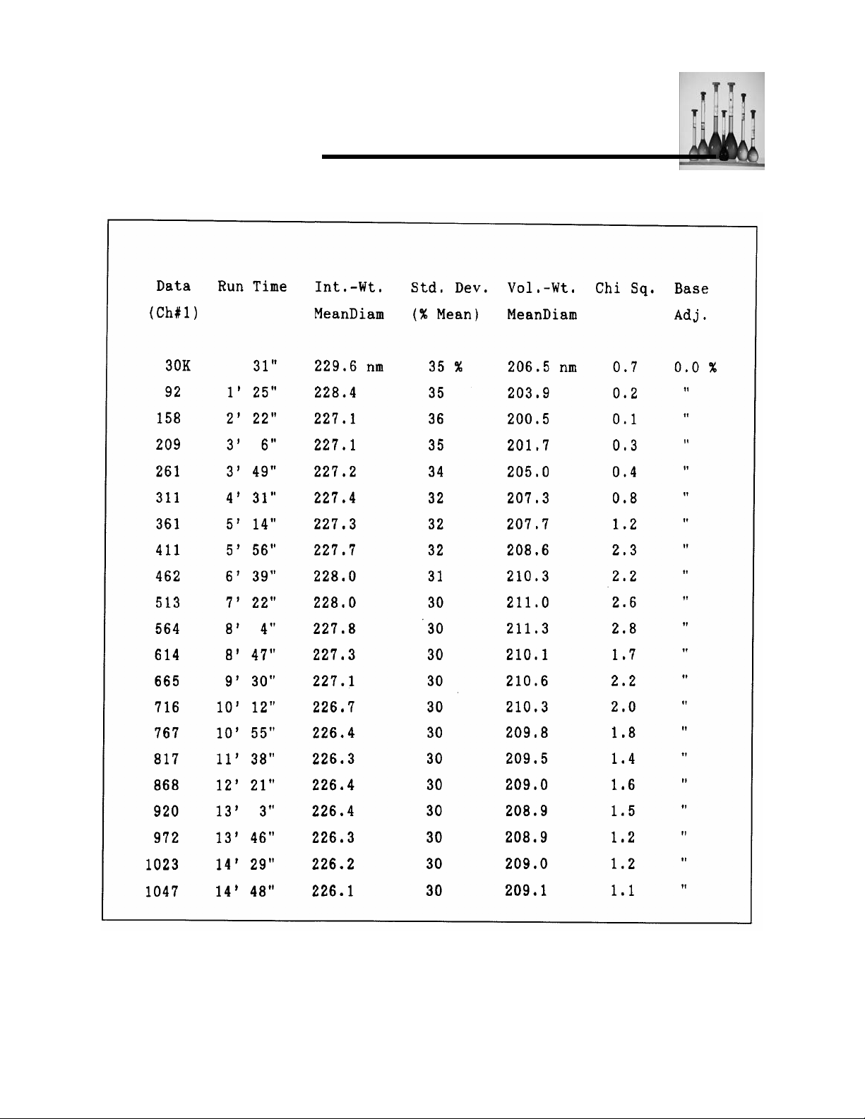
DDLLSS TThheeoorryy

Table 1: Time dependence of the Gaussian analysis results for a typical unimodal sample (IV fat

emulsion)

Nicomp 380 Manual

PSS-380Nicomp-030806

06/06

Page 2 -37

DDLLSS TThheeoorryy

The results shown in Table 1 for a well-behaved fat emulsion nicely illustrate some of the

characteristics of the Gaussian Analysis, discussed earlier. First, we notice that the parameter

Chi Squared cannot be used to judge the stability and/or quality of the fit results if too little data

has been acquired. Here, just 31 seconds into the run, the very low value of Chi Squared is

potentially misleading in suggesting that the Gaussian Analysis has already produced final”

results, of high quality, with settled values of the Mean Diameter and Standard Deviation. In

fact, Chi Squared later increases, to a high of 2.8 at the later time of 8 min 4 see, when

substantial amounts of additional Data have been incorporated into the autocorrelation function

(564K in Channel #1). However, what is meaningful is the fact that this rise is obviously

spurious, since it is followed by consistently lower values; Chi Squared falls back essentially to

unity (1.1) after 13-14 minutes into the run. Clearly, what matters in establishing the validity of

the Gaussian Analysis result for this sample is the fact that Chi Squared remains low with

increasing data acquisition, showing no tendency to grow with time.

Second, we verify from Table 1 that the intensity-weighted Mean Diameter (colt 3) settles very

quickly to a reliable value. After just a couple of minutes, all succeeding values are within 1 % of

the “settled” value of approximately 226nm. On the other hand, the exhibits considerably initial

few minutes of difference is the fact the “settled” value of approx. 226 nm. volume-weighted

Mean Diameter (col. 5) more variation (up to 4%) during the data acquisition. The reason for this

that the Standard Deviation has not yet settled to a constant value. Clearly, a higher degree of

statistical accuracy (i.e. signal/noise ratio) is required in the autocorrelation function to establish

the value of the “curvature” coefficient, a

is needed to fix the value of the linear coefficient, a

observe a 20% variation in the Standard Deviation (coming from a

2% fluctuation in the intensity-weighted Mean Diameter (from a

This affects the results in two ways. First, the relatively large values of the Standard Deviation

(30 to 35% of the Mean Diameter) serve to “push” the volume-weighted Mean Diameter fully

10% below the intensity-weighted value, to approximately 209 nm. Second, because of the

substantial fluctuation in the computed Standard Deviation in the early stages of data

acquisition, the volume-weighted Mean Diameter fluctuates considerably more than does the

intensity-weighted value. However, regarding these fluctuations, a simple rule applies: allow

more time! Obviously, the sample represented in Table 1 is rather well behaved, requiring no

Baseline Adjust and yielding good results very early into the run, close to the final, settled

, in the least-squares quadratic fit (Equation 11), than

2

. Consequently, early into the run, we

1

), as opposed to less than a

2

).

1

Nicomp 380 Manual
PSS-380Nicomp-030806
06/06
Page 2 - 38

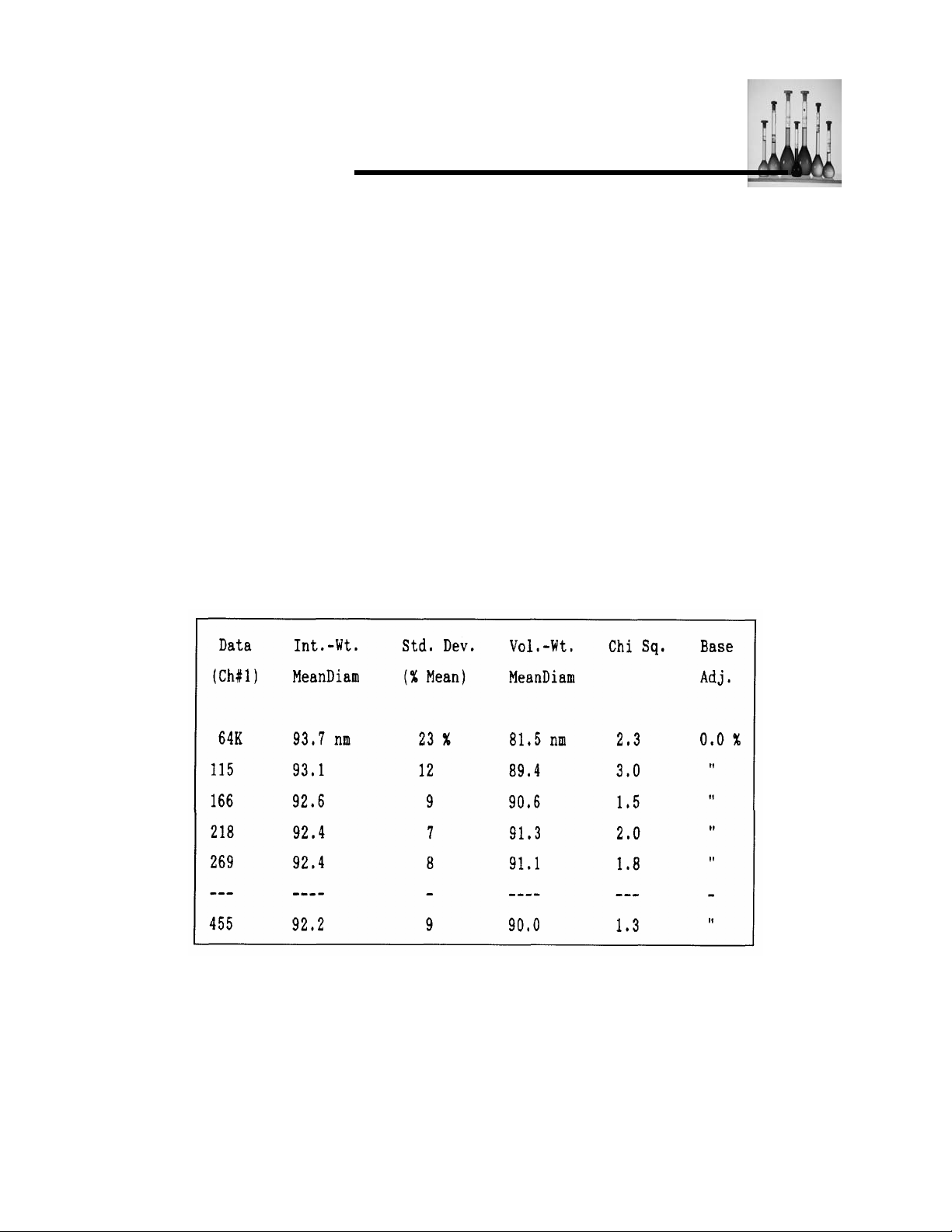
DDLLSS TThheeoorryy

values. Nevertheless, the comments above apply equally well to more “difficult” samples, for

which the results of the Gaussian Analysis show larger fluctuations and require a longer time to

settle.

Next, we examine another sequence of results obtained from the Gaussian Analysis as a
function of accumulating data -- this time returning to the narrow, nearly monodisperse 91nm
latex standard. It is useful to compare these results, summarized in Table 2, with those just
discussed for the broad fat emulsion.

Again, as was found for the broad fat emulsion, the value of Chi Squared is a poor indication of

the extent of settling of the Gaussian Analysis results at the beginning of a run (Data = 64K),

when insufficient data has been collected. The abnormally large value of the Standard Deviation

(23%) the result, again, of insufficient data -- causes the volume-weighted Mean Diameter to be

pushed well below the intensity-weighted value. However, after additional time has elapsed, the

Standard Deviation settles down to 8 or 9%. At this point, there is much less discrepancy

between the two Mean Diameter values, based on the different weightings.

Table 2: Sequence of Gaussian Analysis results obtained for the narrow 91-nm latex
standard

Nicomp 380 Manual

PSS-380Nicomp-030806

06/06

Page 2 -39

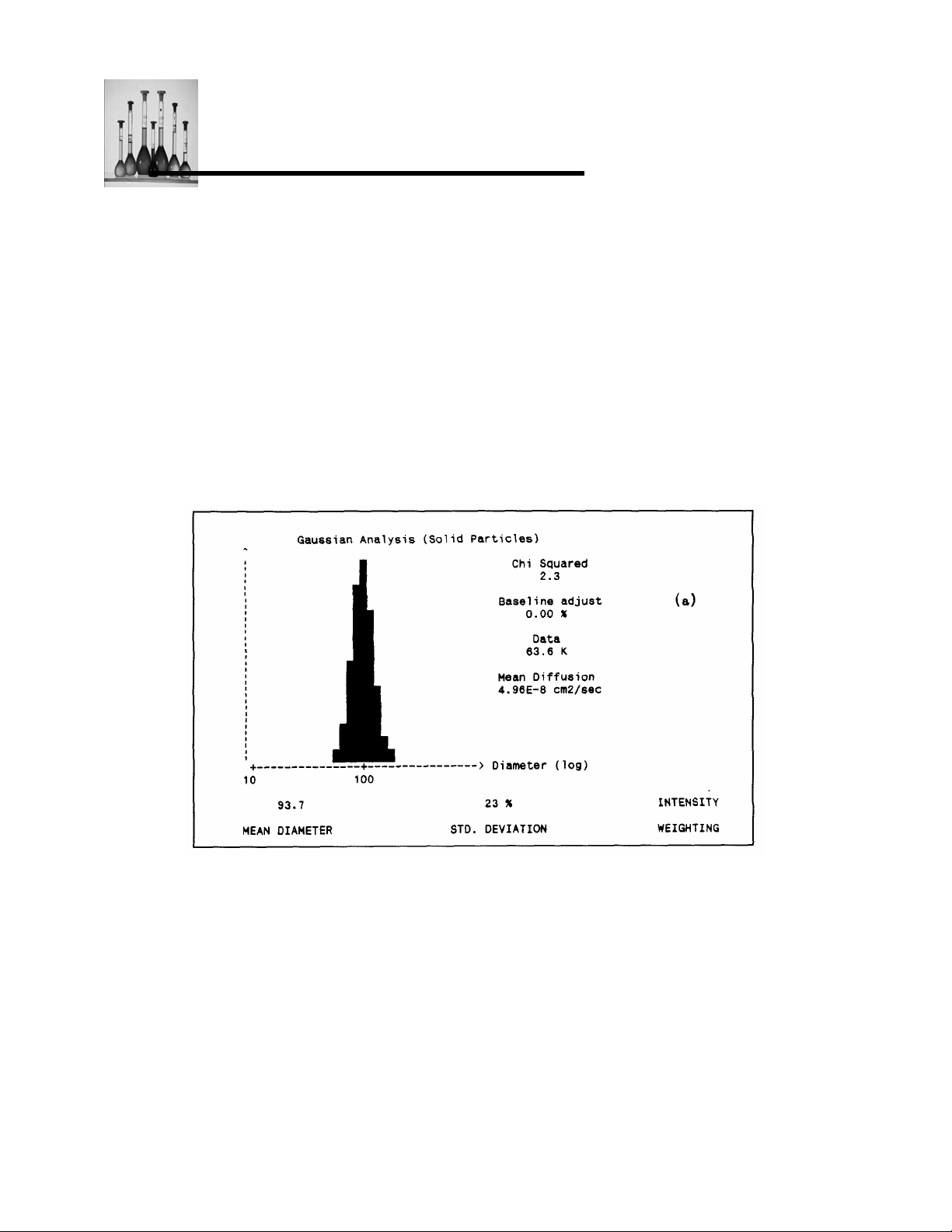
DDLLSS TThheeoorryy

Figures 12a and b show the displays for the intensity and volume-weighted particle size

distributions obtained from the Gaussian Analysis after only 64K of accumulated Data,

equivalent to between one and two minutes of running. By contrast, Figures 12c and d show the

corresponding results obtained with 455K in Channel #1, after approximately 10 minutes. The

latter clearly represent results having a much higher confidence level.

Finally, there is a little-recognized, but significant, attribute of the Gaussian Analysis that

deserves comment here. It often turns out that the computed particle size distribution for a

broad, unimodal population settles more quickly than for a narrow distribution! In the latter case,

one frequently observes results for 91-nm latex after only 64K of Data.

Figure 12a: Intensity-weighted Gaussian Analysis

Nicomp 380 Manual
PSS-380Nicomp-030806
06/06
Page 2 - 40

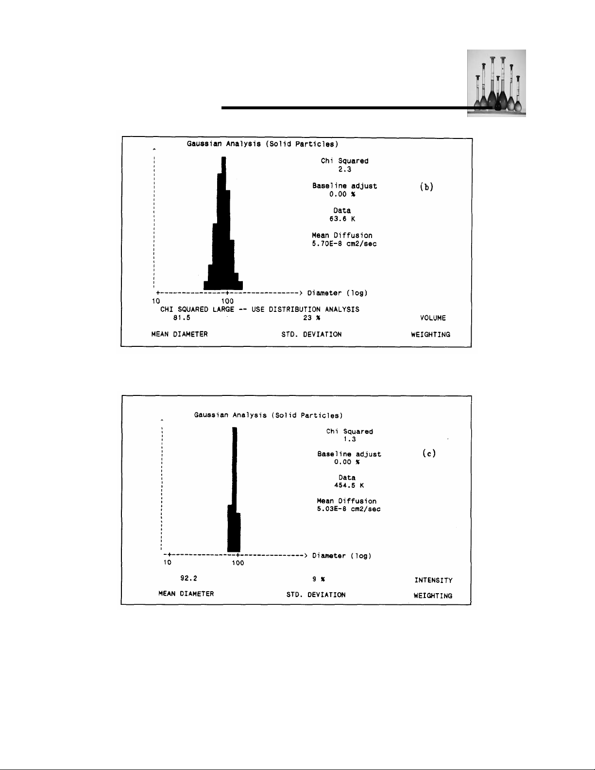
DDLLSS TThheeoorryy

Figure 12b: Volume-weighted Gaussian Analysis

Figure 12c: Intensity-weighted Gaussian Analysis

Nicomp 380 Manual

PSS-380Nicomp-030806

06/06

Page 2 -41

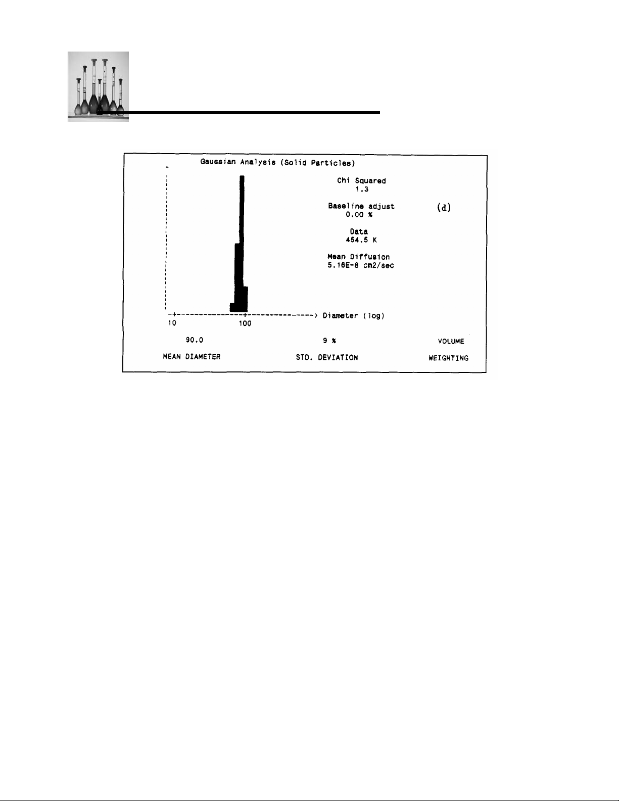
DDLLSS TThheeoorryy

Figure 12d: Volume-weighted Gaussian Analysis results for 91-nm latex after more

Data (455K).

What appear to be large fluctuations in the Standard Deviation-e.g. from 2 % to 12% -- while the

Mean Diameter (with whatever weighting) remains more or less constant. While this factor-of six

variation in the Standard Deviation appears, at first glance, to be very large, it really is not. In

fact, all of the values within that range are effectively nearly equal. Why? Because they all

describe autocorrelation functions which are very close to ideal, single decaying exponentials.

Using Equation 11, we are saying that the ‘curvature represented by coefficient a: is nearly zero

for the above mentioned range of Standard Deviations. There are small changes in the least-

squares quadratic fit (due to tiny fluctuations in the correlation data) which are responsible for

these seemingly large changes in the Standard Deviation. Indeed, these small fluctuations may

be caused by normal Poisson statistics, particle aggregates, “dirt” particles, stray scattered light,

etc. By contrast, broad distributions result in substantial curvature in the quadratic fit (i.e.

relatively large values of a:) and much less sensitivity to small fluctuations in the correlation

data. Hence, in this case, the Gaussian Analysis results are observed to settle relatively more

quickly to a final, reliable “answer”. Typically, it is necessary to start with very “clean”, well

Nicomp 380 Manual
PSS-380Nicomp-030806
06/06
Page 2 - 42

DDLLSS TThheeoorryy

dispersed samples and acquire data for a relatively long time (e.g. 30 to 60 minutes) to obtain

reliable Standard Deviations smaller than 8 to 10% for a sample which is known to be nearly

monodisperse. Under such controlled, ideal conditions, the DLS Module is certainly capable of

yielding single-peak distributions of exceptionally small Standard Deviation.

Nicomp 380 Manual

PSS-380Nicomp-030806

06/06

Page 2 -43

DDLLSS TThheeoorryy

NICOMP DISTRIBUTION ANALYSIS

Rationale for use of the inverse Laplace transform

In the proceeding section we saw that the Gaussian Analysis has the useful attribute that the

resulting distribution settles quickly to a stable, reproducible result with increasing acquisition of

light scattering data. As was pointed out, this is due to the fact that the least-squares quadratic

(cumulants) fit to the reduced data is essentially just a two-parameter fit (apart from a possible

baseline adjustment). Obviously, this “smooth” fit to the data is relatively insensitive to subtle

changes in the autocorrelation constitutes the “good news” Analysis. function. This insensitivity

associated with the Gaussian Analysis.

The “bad news”, of course, is that this method is inherently limited to describing only simple

particle size distributions -- symmetric, single-peak (unimodal) populations. More complex

distributions, such as highly-skewed unimodals or bimodals, are completely misinterpreted by

the Gaussian Analysis; the degree of error will be either quantitative or qualitative, depending

on the precise shape of the true distribution. The only indication of the existence of a more

complicated distribution is the occurrence of a large (and rising) value of Chi Squared, as

described previously. This “warning flag” informs the operator in unambiguous terms that the

Gaussian Analysis result is inappropriate. In this case, another approach for analyzing the data

is clearly needed.

The NICOMP Distribution Analysis provides the needed alternative method for analyzing the

autocorrelation function. In contrast to the Gaussian Analysis, it makes NO a priori assumption

of the shape of the final distribution. Rather than relying on only two parameters (plus, possibly,

a baseline adjustment), the Distribution Analysis typically yields as many as three, or even four,

independent parameters, as well as a baseline adjustment. Because the amount of information

(i.e. the number of parameters) potentially provided by the Distribution Analysis exceeds that

yielded by the Gaussian Analysis, considerably more data is needed in general in the

autocorrelation function to obtain a reliable result. This is simply a requirement of better

statistical accuracy, or signal to-noise ratio, in the autocorrelation function. In this game, which

is inherently mathematical, a simple rule applies: you cannot obtain something for nothing!

Nicomp 380 Manual
PSS-380Nicomp-030806
06/06
Page 2 - 44

DDLLSS TThheeoorryy

Obtaining more information relating to a more complex distribution requires that more time be
expended acquiring more scattered intensity data. While this same rule was implicit in our

discussion of the settling of the Gaussian Analysis results, we shall see that it is much more

critical in the case of the Distribution Analysis.

The general mathematical procedure that is utilized in the proprietary NICOMP Distribution

Analysis is referred to as inversion of the Laplace transform (“ILT”). This rather sophisticated

technique has also been used to analyze a variety of problems in other scientific areas,

unrelated to light scattering. The specific mathematical procedure is a more sophisticated

version of the least-squares calculation used in the Gaussian (cumulants) Analysis; it is referred

to as nonlinear least-squares (“NLLS”) analysis.

We can appreciate the problem which must be solved by the ILT technique by considering the

most general expression for the autocorrelation function, C(t’), corresponding to an arbitrary

distribution of particle sizes. We recall for the trivial example of a single particle size that C(t’) is

simply an exponentially decaying function, given by Equations 7 and 8, or 10a and b. This is

now replaced by a more general expression, containing a weighted sum of individual

exponentially decaying functions, each of which corresponds to a different particle diameter:

2

⎧

′

⎨

∑

=Mi

1

⎩

−=

⎫

2

′

)exp()(

tKDfAtC

(14)

⎬

ii

⎭

Here, again, the baseline of the autocorrelation function (t’→∞) is given by B. and constant A

simply relates to the total amount of data acquired in “channel #0” (t’ = 0) of C(t’), such that

C(O)=A+B.

In Equation 14 above we have assumed a discrete distribution of particle sizes, containing M

different diameters, each labeled by index i (running from 1 to M). The diffusion coefficient for

each particle diameter is given by D

Einstein relation, Equation 2. The constants f

the individual exponentially decaying functions, exp(-D

the different particle diameters present in the sample solution (of this, more later). In the trivial

case of a single, uniform particle size, Equation 14 reduces to C(t’) =A(f

which is exactly the same as Equation 7 or l0a and b, provided that the constant A(f

the previous prefactor, A.

, which is obtained from the radius Ri using the Stokes-

i

are the weighting coefficients which mix together

i

K2t’), according to the relative amounts of

i

)2exp(-2D1K2t’) + B ,

1

)2 replaces

1

Nicomp 380 Manual

PSS-380Nicomp-030806

06/06

Page 2 -45

DDLLSS TThheeoorryy

The goal of the ILT technique is to solve Equation 14. The quantity which is

hand side, the measured autocorrelation function C(t’) (where t’ is given by the discrete
channels t’ = Δt’, 2Δt’, …, 64 Δt’). The unknowns are the M individual weighting coefficients f

buried in the summation on the right hand side of Equation 14. This multi-variable equation must

therefore be “inverted” in order to yield the “answer”, which is the set of weighting coefficients fit

Equation 14 is, in fact, the discrete representation of a more general integral equation that

defines the Laplace transform. To appreciate this, we can define a new “reduced”

autocorrelation function H(t’), obtained from the original C(t’): H(t’) = {(C(t’)-B)/A}

We also define a new variable, s, which is simply proportional to the diffusion coefficient

variable D : s = DK

2

(with K given by Equation 9). Using these new definitions we can recast

Equation 14 in its integral form, in which there are an infinite number of different particle

diameters. Equation 14 therefore becomes,

∞

(15)

′

∫

0

′

−=

)exp()()( dstssftH

where s (or D) ranges from zero (corresponding to an arbitrarily large particle) to infinity

(corresponding to a particle of diminishing small diameter). The above expression defines the

integral Laplace transform of H(t’), which is the desired weighting function f(s).

Returning to Equation 14. we must use an ILT technique to obtain the best possible estimates

for the weighting coefficients f

. The details of the mathematical procedure used to perform the

i

discrete Laplace transform inversion of the autocorrelation data in the NICOMP Distribution

Analysis are beyond the scope of this manual -- and, in any case, are proprietary. Suffice to say

that the procedure represents a variation on other ILT methods discussed in the light scattering

literature -- most especially, that developed by S. Provencher. The ways in which the NICOMP

procedure differs from this and other methods relate mainly to the manner and extent of

smoothing carried out within the mathematical “algorithm”.

known is the left-

1/2

.

,

i

Nicomp 380 Manual
PSS-380Nicomp-030806
06/06
Page 2 - 46

DDLLSS TThheeoorryy

It is most important to appreciate the practical limitations inherent in any solution of Equation 14

using an ILT algorithm. In principle, one would like to be able to obtain, with reasonable

accuracy, all values f

true particle size distribution. In practice, however, one falls far short of this goal. Typically, it is

possible to obtain a stable distribution containing one, two or even three peaks. In the case of

two peaks, we obtain two values of peak diffusion coefficients, D

strength parameter, f

adjust). Note, in all of the distribution results of the DLS Module, the maximum height of any

distribution is always normalized to 100; hence, in the case of two peaks, only the ratio of their
heights is an independent parameter.) In the case of three peaks, one will obtain three peak D

values-D

, D2 and D

1

(there are M of them), thereby obtaining a faithful representation of the

i

and D

1

, for a total of three independent parameters (in addition to the baseline

2/f1

-- and two relative strength parameters, f

3

,/f1 and f3/f1.

2

, , and one relative

2

Nicomp 380 Manual

PSS-380Nicomp-030806

06/06

Page 2 -47

DDLLSS TThheeoorryy

The Nicomp allows one to establish the set of diameter values, I =1 to M, over which Equation
14 is defined. The total number, M, is given by the PLOT SIZE; the values vary from
MIN.DIAM.(i=l) to RANGE * MIN.DIAM.(i=M). In most cases it is desirable to use the
logarithmic diameter scale, in which the individual diameter “slices” are spaced logarithmically.
Each of the diameter values is converted to a diffusion coefficient, Di; the resulting individual
decaying exponential functions in Equation 14, exp(-DiK2t’) , constitute the starting “basis
vectors for the NICOMP ILT algorithm. The latter systematically varies the weighting
coefficients fi in Equation 14 in order to determine the sensitivity of the resulting computed fit
(to C(t’)) to each coefficient. In this way, many, if not most, of the coefficients are set equal to
zero. The non-zero values of fi which survive constitute the “solution” to Equation 14. As
additional data are acquired in C(t’), this solution will change -- either a little or a lot, depending
on the current statistical accuracy of C(t’).

There is an additional observation concerning the ILT fitting procedure and Equation 14 that is

VERY IMPORTANT. The weighting coefficients f

represent the relative scattering intensities

i

contributed by particles of size type i. That is, the individual decaying exponential functions

corresponding to each particle diffusivity D

factors f

, each of which is proportional to the total scattered intensity produced by all of the

i

, are added together in Equation 14 with weighting

i

particles of that size. From the discussions in the previous sections, we have:

f

∝ Ni (Vi)2 (Gi)

i

2

(16)

where Ni is the total number of particles of (size) type i, and V

to scattering. In the case of a solid particle, V

∝ (di)3; for a thin-walled vesicle, V

i

the following section.) The extra factor for the additional effects of intra-particle (G

interference, important when the particle diameter is no longer negligible compared to the laser

wavelength (Mie region). In the small diameter Rayleigh region (diameters smaller than about

50 nm), G

is essentially unity for all particle shapes and sizes and can be ignored in Equation

i

16.

We have explicitly written the expression for the weighting coefficients f

motivate Equation 14, which is the basic starting point for Distribution Analysis. We must

is the particle volume giving rise

i

)2, (See

i ∝ (di

)2 accounts

i

in Equation 16 to help

i

Nicomp 380 Manual
PSS-380Nicomp-030806
06/06
Page 2 - 48

DDLLSS TThheeoorryy

remember, of course, that the coefficients f

are the unknowns; they are computed by inverting

i

Equation 14. The “answer” produced by Distribution Analysis is the intensity-weighted particle

size distribution: a plot of f

vs di (diameter). The di scale is determined by the choices of

i

MIN.DIAM., PLOT SIZE and RANGE, as discussed earlier.

The volume- and number-weighted distributions are obtained from the intensity-weighted plot by

dividing each value of f

by Vi(Gi)2 and (Vi)2(G1)2, respectively, for each diameter “slice”. It is for

i

this reason that Equation 16 is needed, to permit the various weightings to be obtained from the

“raw” intensity weighted distribution of f

values which emerges from the ILT algorithm.

i

To conclude this Section, remember that the actual plots obtained from the Distribution Analysis

represent very simplified versions of whatever the true particle size distribution may be. The

statistical accuracy that can be realistically achieved in the underlying autocorrelation data

simply cannot support an analysis which reliably yields any more “detail” in the distribution.

However, it usually turns out that the resolution and accuracy of the NICOMP algorithm are

sufficient to yield a meaningful representation of the true particle size distribution for many

systems of practical significance.

A simple test of Distribution Analysis: uniform particle size (latex)

In order to investigate the capability of the NICOMP Distribution Analysis, we must apply it to a

polydisperse sample which differs qualitatively from those investigated earlier-i.e. those

consisting of simple unimodal populations which could be well characterized using the Gaussian

Analysis. First, however, we should check the performance of the new algorithm using a narrow,

nearly-monodisperse polystyrene latex standard. For such a sample, it must be able to

determine the mean particle diameter with high accuracy.

In Figure 13 we see the video display of the volume-weighted distribution obtained for the 91nm

latex standard. The corresponding result obtained using the Gaussian Analysis was shown

earlier in Figure 12d. We find a mean diameter of 88.8 nm for Figure 13, compared

Nicomp 380 Manual

PSS-380Nicomp-030806

06/06

Page 2 -49

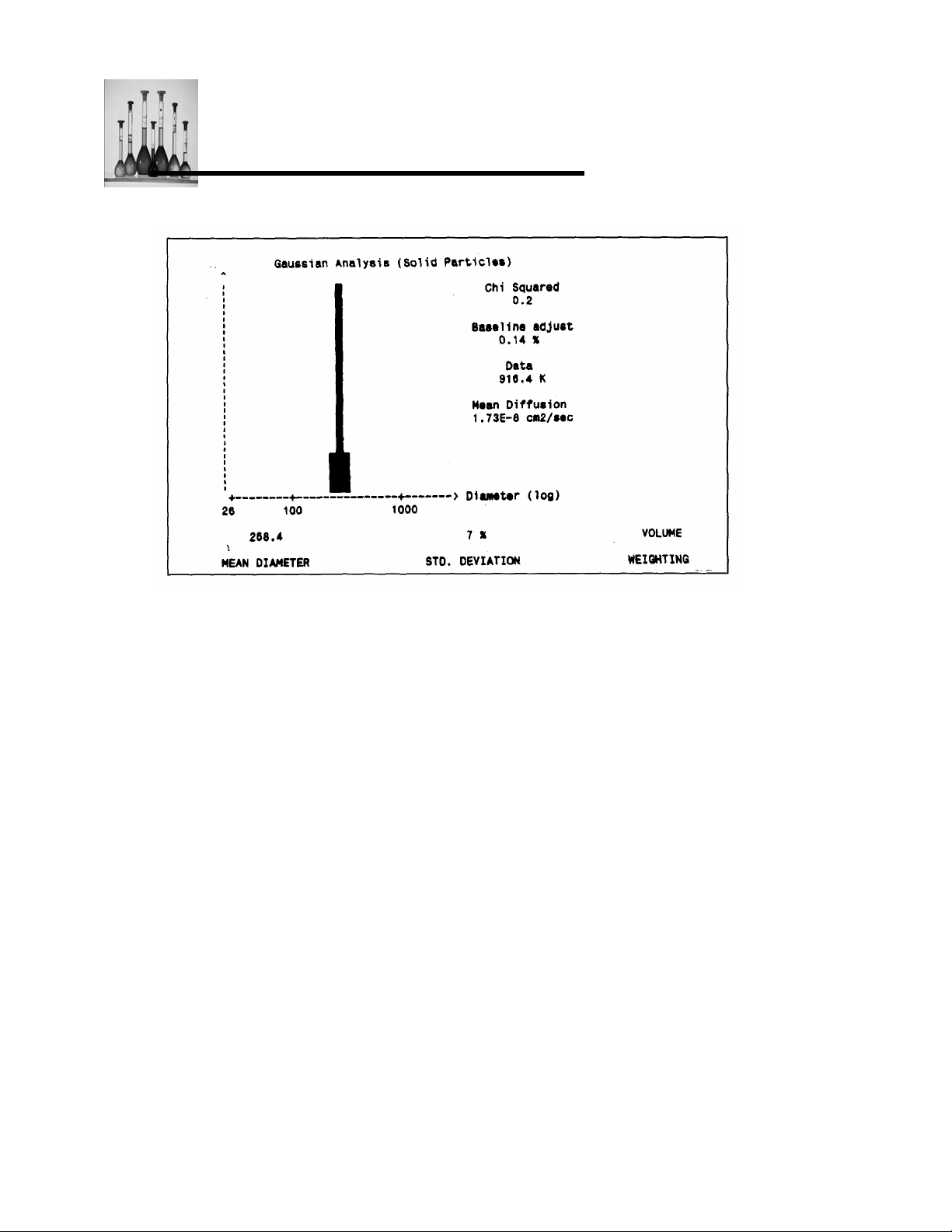
DDLLSS TThheeoorryy

Figure 13: Volume-weighted Distribution Analysis result for 91-nm latex standard

to 90.0 nm for the Gaussian Analysis result. This discrepancy (only 1 %) is excellent,

considering the fact that two radically different mathematical procedures were used to obtain the

two results. (It was pointed out earlier that the true diameter of this standard lies closer to 88-89

nm, rather than the nominal 91-nm value.)

In Figure 13 we see that the Fit Error for this analysis fell to 4.60 with 480K of Data (Ch. #1).

This value should continue to decrease with increasing data acquisition. It is IMPORTANT to

appreciate that the Fit Error only provides an indication of how relatively stable, or settled, the

Distribution Analysis results should be, but NOT on whether it is the preferred result, compared

to the Gaussian Analysis. This judgment, of course, is provided by the value of Chi Squared. As

the warning message clearly states, in this case the Gaussian Analysis must be used.

One will typically find that narrow, ideal distributions like this one will settle relatively quickly--i.e.

with values of Fit Error of 3 or 4 or higher. However, in general one should run long enough to

achieve a value below 2.0 in the case of a “clean’, single-peak distribution. For more complex

distributions, it is usually advisable to achieve a Fit Error below 1.5, or even approaching 1.0, to

Nicomp 380 Manual
PSS-380Nicomp-030806
06/06
Page 2 - 50

DDLLSS TThheeoorryy

obtain the most accurate, reproducible results. (As a point of reference, one can typically

achieve a Fit Error of 0.1 or 0.2 after 8 to 12 hours of data collection.) Again, this parameter only

characterizes the stability of the resulting answer, and NOT its appropriateness vis-a-vis the

simpler Gaussian Analysis result.

In Figure 13 we find an ideal value for the Residual: 0.0. We therefore conclude that there is a

negligible concentration of aggregates or other large-particle contaminants in the sample

suspension. In the event that the value for the Residual is significant, e.g. 10 or larger, one of

two possibilities will occur with increased data acquisition. 1) The Residual will simply remain

high, with little change in the composition of the size distribution plot; 2) The Residual will fall to

zero, resulting either in a shift in the position(s) of the peak(s) (usually to higher diameter(s)), or

in the appearance of a new peak at the high end of the diameter scale. The latter explicitly

reveals the large-size component previously signaled (in #1) by the large value of the Residual.

In the early stages of data acquisition these two possibilities frequently alternate in seemingly

random fashion, because of inadequate statistical accuracy in the autocorrelation function.

Obviously, it is desirable to achieve result #2 above -- a zero Residual. One can often hasten

the transition from #1 to #2 by increasing the maximum value of the diameter scale, equal to

MIN.DIAM. * RANGE. This is accomplished by increasing the value of RANGE (e.g. to 500 or

1000, if necessary).

Nicomp 380 Manual

PSS-380Nicomp-030806

06/06

Page 2 -51

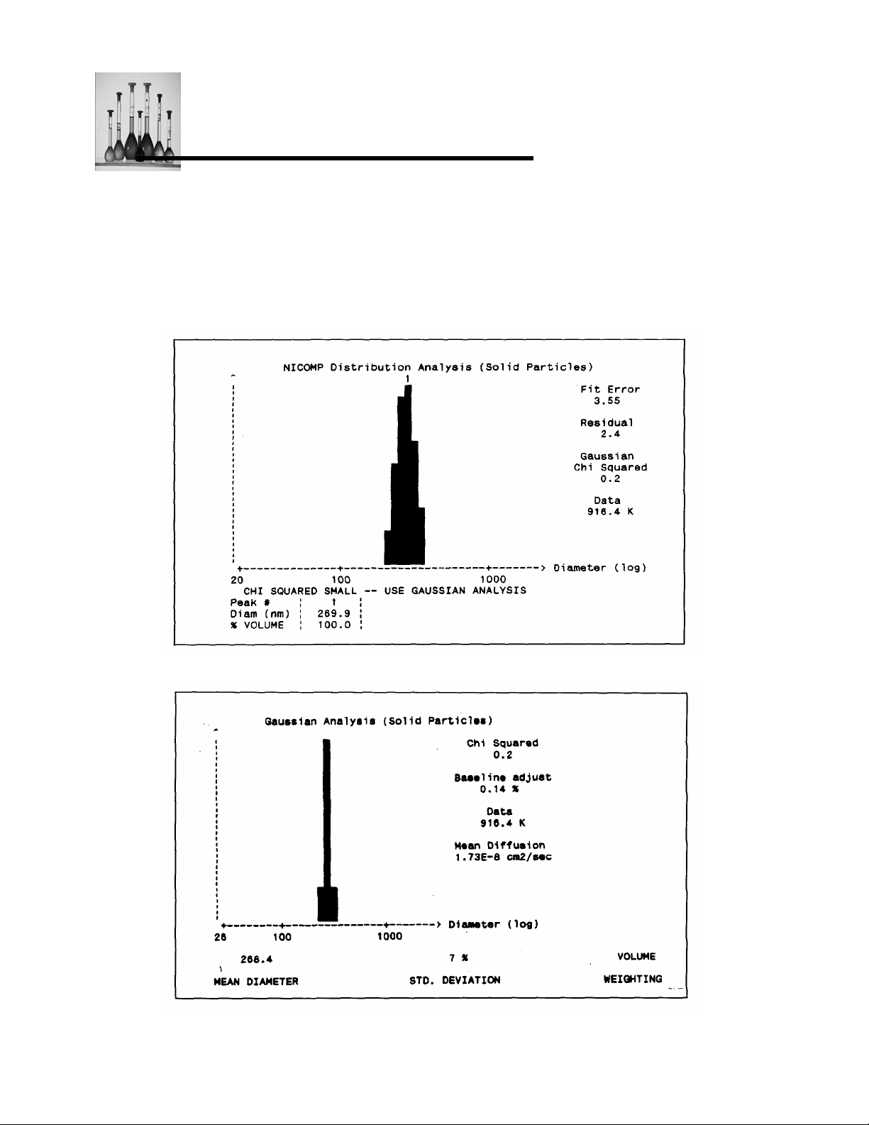
DDLLSS TThheeoorryy

In Figure 14a we show a typical result obtained using Distribution Analysis for a larger size

polystyrene latex standard 261 nm. Here, we obtain a volume-weighted mean diameter of 269.9

nm, which agrees very well with the value found using Gaussian Analysis, 268.4 nm, shown in

Figure 14b (with the same Data).

Figure 14a: Volume-weighted Distribution Analysis result for 261-nm latex standard

Nicomp 380 Manual
PSS-380Nicomp-030806
06/06
Page 2 - 52

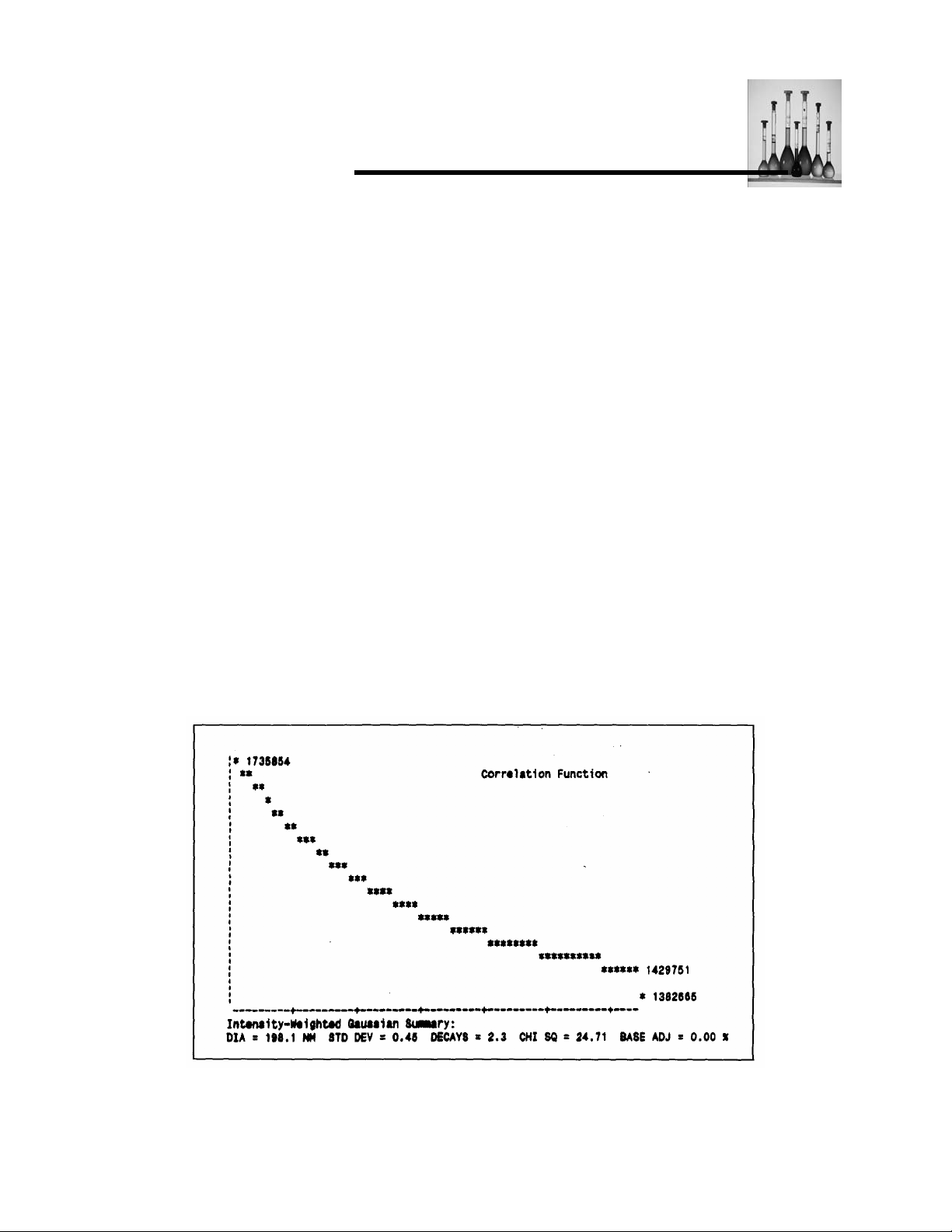
DDLLSS TThheeoorryy

Figure 14b: Volume-weighted Gaussian Analysis result for 261-nm latex standard
(See Figure 14a.)

It is most important for one to appreciate the fact that reliable estimates of the widths of peaks in

the particle size distribution CANNOT be obtained using the Distribution Analysis. The peak

widths obtained from this procedure depend on details of smoothing and basis-vector coupling

in the ILT algorithm, as well as the operator’s choice for the SMOOTHING parameter. On the

other hand, it should now be clear that the Gaussian Analysis does, indeed, yield a reliable

estimate of the peak width -- as in Figure 14b -- provided Chi Squared is low, indicating a good

fit.

A harder test for Distribution Analysis: a bimodal distribution (latex)

We now consider the first difficult test of the NICOMP ILT procedure -- analysis of a bimodal

distribution. Figure 15 shows the autocorrelation function after 23 minutes for a bimodal sample

prepared using the 91 and 261 nm latex standards investigated earlier. This test bimodal was

made using a 3:1 ratio by mass (or volume) in favor of the 91 nm latex, so as to enhance the

relative scattering contribution of the smaller-size component t more later). Figure 16 shows a

plot of the logarithm of the reduced autocorrelation data, C(t’)-B vs t’ (channel #), with a straight

line drawn for reference purposes.

Figure 15: Autocorrelation function for a test bimodal: 3:1 (vol.) ratio, 91 and 261 nm

Nicomp 380 Manual

PSS-380Nicomp-030806

06/06

Page 2 -53

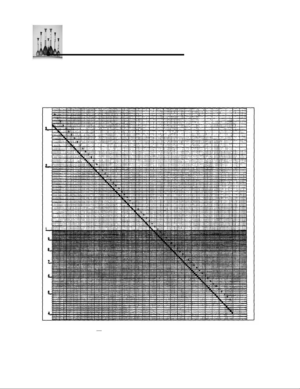
DDLLSS TThheeoorryy

latex particles

Figure 16: Loge( C(t’)-B) vs t’ for data of Figure 15

It is perhaps surprising to see that autocorrelation curve in Figure 15 does not the share of the

Nicomp 380 Manual
PSS-380Nicomp-030806
06/06
Page 2 - 54

DDLLSS TThheeoorryy

appear to differ appreciably from that observed previously for the broad, unimodal fat emulsion

of Figure 9a. Here we have particle sizes which differ by almost a diameter. We therefore would

expect to see evidence of a “breakpoint”, or “knee”, in the logarithmic plot of the reduced

Nicomp 380 Manual

PSS-380Nicomp-030806

06/06

Page 2 -55

DDLLSS TThheeoorryy

autocorrelation data (Figure 16), given the admixture (Equation 14) of two exponential functions

whose decay time constants differ by a factor of three. However, NO such breakpoint is evident

in Figure 16. Indeed, the curvature in the reduced data in Figure 16 qualitatively resembles that

seen for the broad unimodal emulsion in Figure 9b.

Nicomp 380 Manual
PSS-380Nicomp-030806
06/06
Page 2 - 56

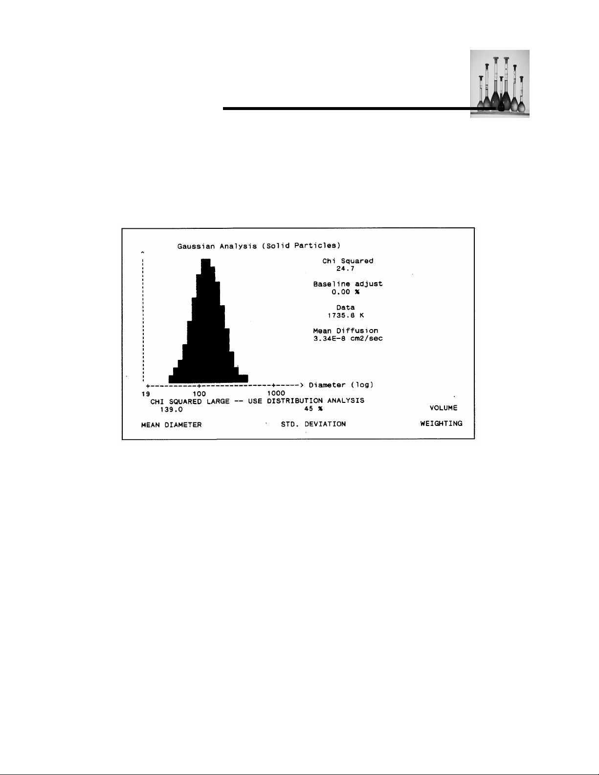
DDLLSS TThheeoorryy

Suppose we were to analyze this new system as we did the emulsion, using the Gaussian

Analysis. From the substantial curvature evident in Figure 16, we would expect the unimodal

generated by the Gaussian Analysis to possess a large standard deviation -- i.e. to be very

broad. This is indeed the case, as seen in Figure 17.

Figure 17: The volume-weighted Gaussian Analysis result corresponding to Figure 15
and Figure 16

The volume-weighted mean diameter is 139 nm, with a standard deviation of 45%. (We also

obtain the expected result that the volume-weighted mean diameter is pulled down substantially

below the intensity-weighted value -- 198 nm from Figure 15 -- owing to the large standard

deviation.) Figure 17 would have represented the state of the art of DLS-based particle sizing

technology only 10 years ago, prior to the commercial introduction of ILT algorithms for analysis

of highly polydisperse distributions. Of course, we recognize that the Gaussian Analysis result is

probably seriously flawed, given the large value of Chi Squared -- 24.7 -- and the fact that it was

observed to increase continually (and dramatically) with increasing data acquisition. The

appropriate warning message is prominently displayed in Figure 17.

Notwithstanding the apparent qualitative resemblance of the autocorrelation data for the broad

unimodal emulsion and the bimodal latex suspension, the NICOMP Distribution Analysis has

little difficulty revealing the true nature of the latter sample. Figure 18a clearly shows a bimodal

Nicomp 380 Manual

PSS-380Nicomp-030806

06/06

Page 2 -57

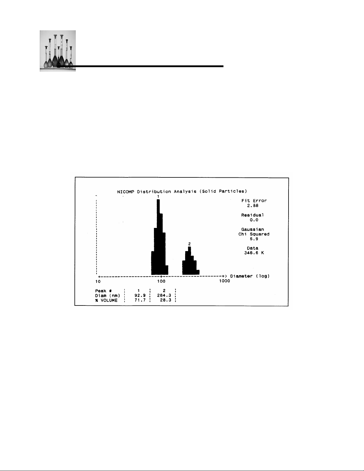
DDLLSS TThheeoorryy

distribution, which is surprisingly close to the correct result, given the relatively small amount of

data acquired (Data = 374K). It yields volume-weighted peak mean diameters of 92.9 and 284.3

nm, which are close to the nominal values of 91 and 261 nm. Of course, more data need to be

acquired before one can be confident that the Distribution Analysis result has reached a stable

solution; the Fit Error value of 2.88 is still too high, providing a cautionary signal. Nevertheless,

with this small amount of data the value of Chi Squared for the alternative Gaussian Analysis

has already climbed to 5.9. The values of % volume found for the two peaks, 71.7 and 28.3, are

very close to the actual values of 75 and 25 % (for a 3:1 volume ratio).

Figure 18a: The volume-weighted Distribution Analysis result for the 3:1 91/261 nm
test bimodal after Data = 347K

The distribution obtained after more than 10 minutes of running (Data = 840K) is shown in

Figure 18b. The peak locations and relative volume percentages have changed somewhat

relative to the results of Figure 18a. By this time the Gaussian Chi Squared has risen further, to

8.2, and the Fit Error has fallen to 1.84. The non-zero value of the Residual suggests that

additional data acquisition would be desirable.

Nicomp 380 Manual
PSS-380Nicomp-030806
06/06
Page 2 - 58

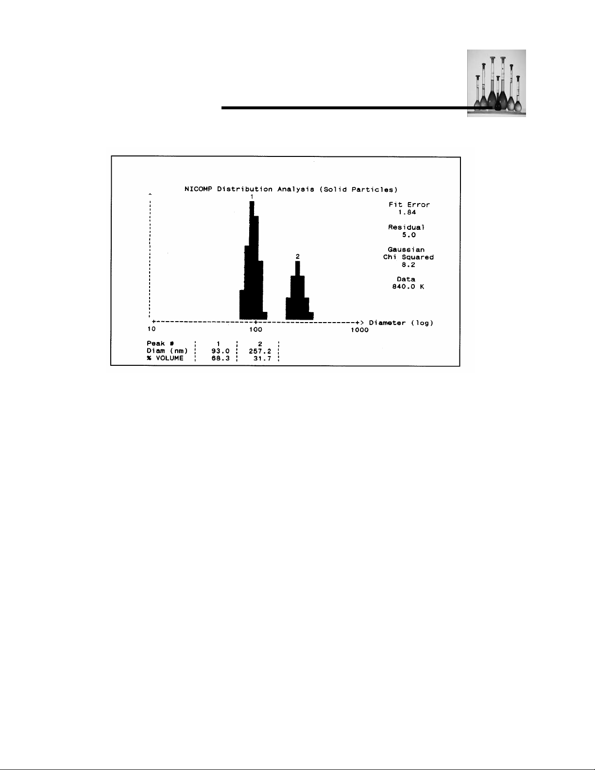
DDLLSS TThheeoorryy

Figure 18b: The volume-weighted Distribution Analysis result for the test bimodal
after Data = 840K (10 mm.)

Figure 18c shows the volume-weighted Distribution Analysis result for the same test bimodal

after 23 minutes elapsed time. Now, the Fit Error has fallen close to 1.0, and the Residual has

returned to its ideal value of 0.0. Chi Squared has grown to 24.7, which unambiguously rules out

acceptance of the Gaussian Analysis result. The mean diameters of the peaks are now at 94.2

and 283.4 nm. While these values are too high by a few percent, a closer examination of the

printouts (shown below) reveals that the “error” represents diameter displacements of less than

one diameter “slice” for each peak. This is an exceptionally good performance, given the

difficulty of this test sample. Indeed, the alternative ILT algorithms being used today generally

perform much less well when faced with a control sample like this one. We have deliberately

showed typical results obtained by the DLS Module for this 3:1 91/261 nm test bimodal after 20-

30 minutes running time; on occasion, even better accuracy has been attained.

Nicomp 380 Manual

PSS-380Nicomp-030806

06/06

Page 2 -59

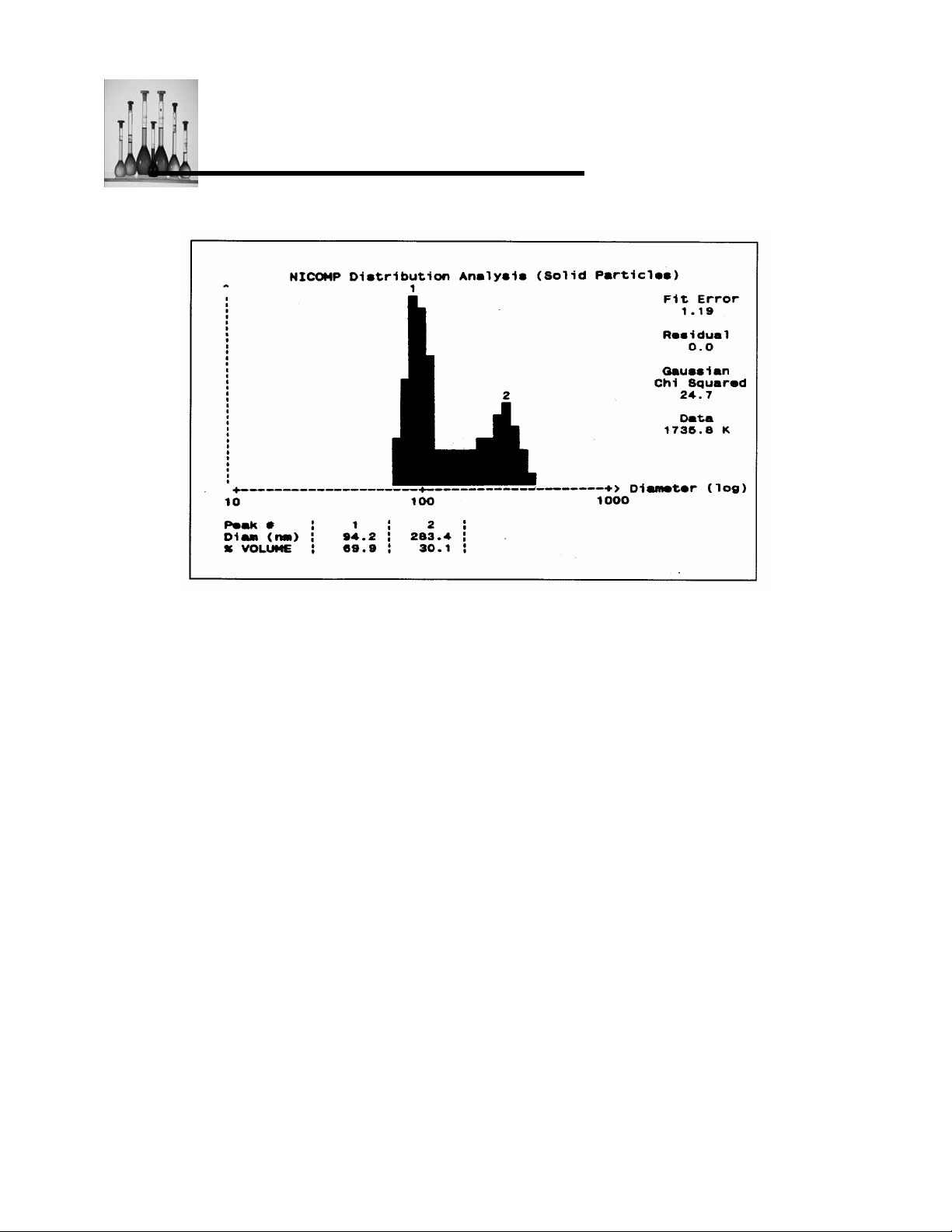
DDLLSS TThheeoorryy

Figure 18c: The volume-weighted Distribution Analysis result for the test bimodal after
Data = 1736K (23 mm.)

Now it is instructive to show a plot of the intensity-weighted distribution -- i.e. the set of

weighting coefficients f, in Equation 14 -- which corresponds to the result just discussed. This is

shown in Figure 18d. As taught earlier, this is the fundamental result which emerges from the

Distribution Analysis; all of the more useful weightings are derived from Figure 18d using the

rules of light scattering (Equation 16).

Nicomp 380 Manual
PSS-380Nicomp-030806
06/06
Page 2 - 60

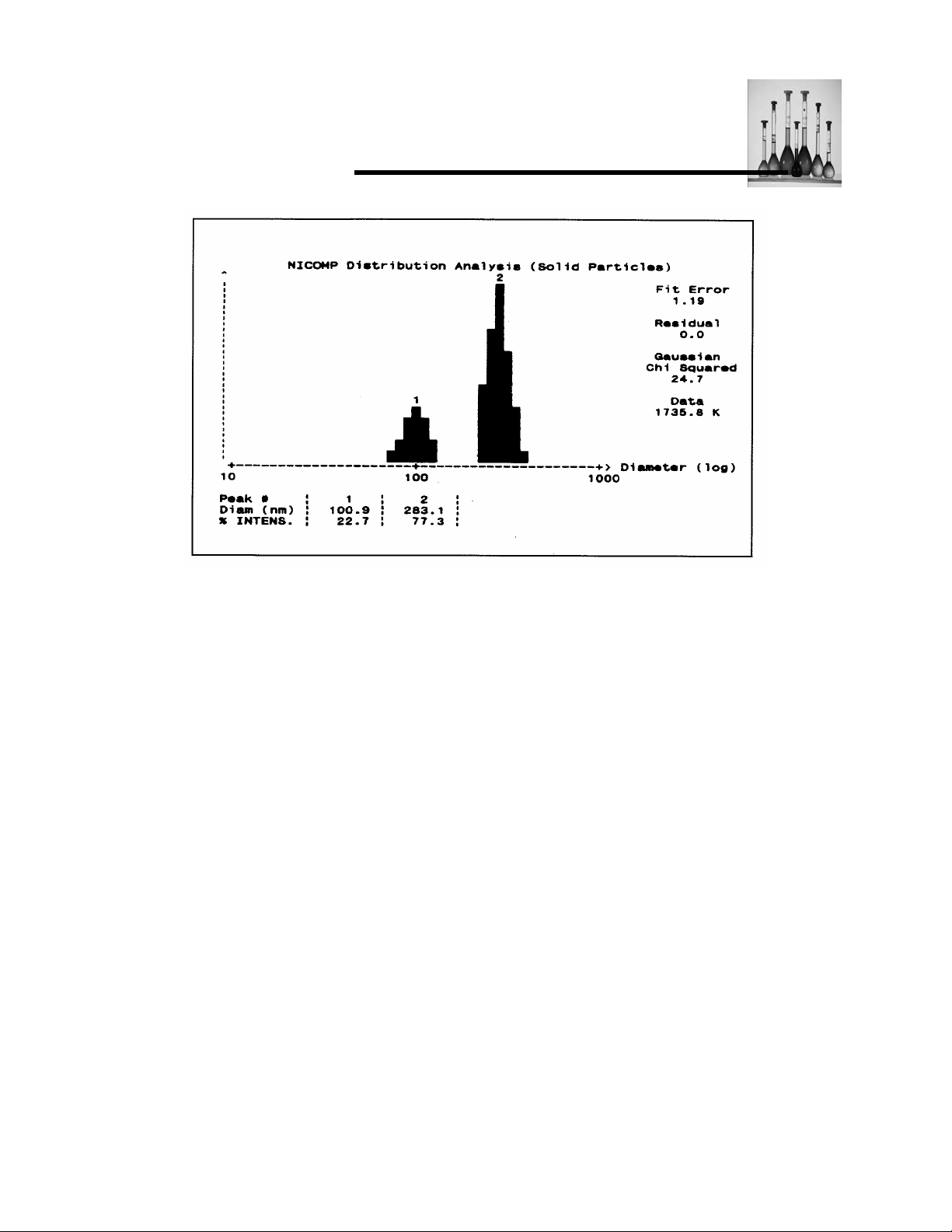
DDLLSS TThheeoorryy

Figure 18d: The intensity-weighted Distribution Analysis result for the test bimodal,
corresponding to Figure 18c

We now can appreciate why the test sample was deliberately skewed at the start toward the

smaller-diameter particles. Even though there is three times as much latex mass, or volume,

contained in the 91 nm component, compared to the 261 nm size, fully three-fourths of the total

scattered light (computed by inverting Equation 14) is produced by the 261-nm fraction. Had we

attempted to analyze a simple 1:1 mixture of the two sizes, the algorithm would still have found

a bimodal distribution, but would have had a harder time correctly establishing the mean

diameters of the two peaks, especially the weaker one (91 nm). Although we appear to have

obtained the excellent results of Figures 18a-d with relative ease, the user should be warned

that this analysis is a difficult one. Failure to disperse adequately the latex particles or to

achieve a dirt-free suspension will in general cause the quality of the Distribution Analysis

results to deteriorate markedly. Most of the commercially available DLS particle sizing

instruments find it more difficult to achieve results on a routine basis like those seen in Figures

18a-d.

Nicomp 380 Manual

PSS-380Nicomp-030806

06/06

Page 2 -61

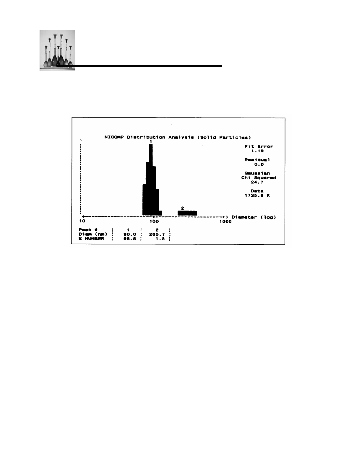
DDLLSS TThheeoorryy

The number-weighted distribution corresponding to the above plots is shown in Figure 18e. It is

obtained from the volume-weighted result as described earlier, using Equation 16.

Figure 18e: The number-weighted Distribution Analysis result for the test bimodal,
corresponding to Figures 18c,d

see in Figure 18e that the mean peak diameters are very close to the nominally correct values

for this simplest of weightings. However, we can also appreciate why this choice of weighting is

often avoided, and volume weighting chosen in its place. For any highly polydisperse

distribution, such as the present one, there is usually too large a disparity between the numbers

of smallest and largest particles. We find here that the 91 nm particles represent over 98% of

the total number, with the 261 nm species accounting for only 1.5%. The resulting plots on a

linear scale lose accuracy because of this very strong skewing toward the smallest-particle peak

in the distribution. Figures 19a,b and c show the detailed printout summaries for the three

weightings corresponding, respectively, to the intensity-, volume- and number-weighted

distributions.

It should be evident from our earlier discussion of the motivation behind the ILT algorithm that

the closer the spacing of the two peaks in a bimodal, the more unlikely it is that the Distribution

Analysis will produce the right answer. As seen in Figure 16, even when there is a 3-fold

Nicomp 380 Manual
PSS-380Nicomp-030806
06/06
Page 2 - 62

DDLLSS TThheeoorryy

separation of the two sizes, the autocorrelation function bears a close qualitative resemblance

to that obtained from a broad unimodal distribution. In practice, the NICOMP ILT algorithm is

able to resolve a bimodal having a size separation of 2:1, or even somewhat closer, provided

the sample is “clean” -- i.e. largely free of aggregates and other large-particle contaminants. (Of

course, this capability presupposes that there is a reasonably well-balanced intensity

contribution from each species.) In general, the narrower the separation, the more data are

needed to permit unambiguous resolution of the bimodal, including a large value of the

Gaussian Chi Squared. Even for a widely-spaced bimodal, however, one must always keep in

mind the practical requirement that the weakest peak contribute adequate intensity. The “rules”

of light scattering, as summarized by Equation 16, will alert one to the possibility that a bimodal

cannot be measured -- NOT because of insufficient volume fraction for a given size component

(typically the smaller size), but because that component contributes only 1 % or less to the total

scattered intensity. As a general rule of thumb, we can say that a second (or third) peak will be

reliably measured only if its relative intensity is at least 1-2%. Hence, whenever one is using the

Distribution Analysis, it is usually a good idea to obtain a printout of the intensity-weighted

result, as well as the desired volume-weighted plot.

Nicomp 380 Manual

PSS-380Nicomp-030806

06/06

Page 2 -63

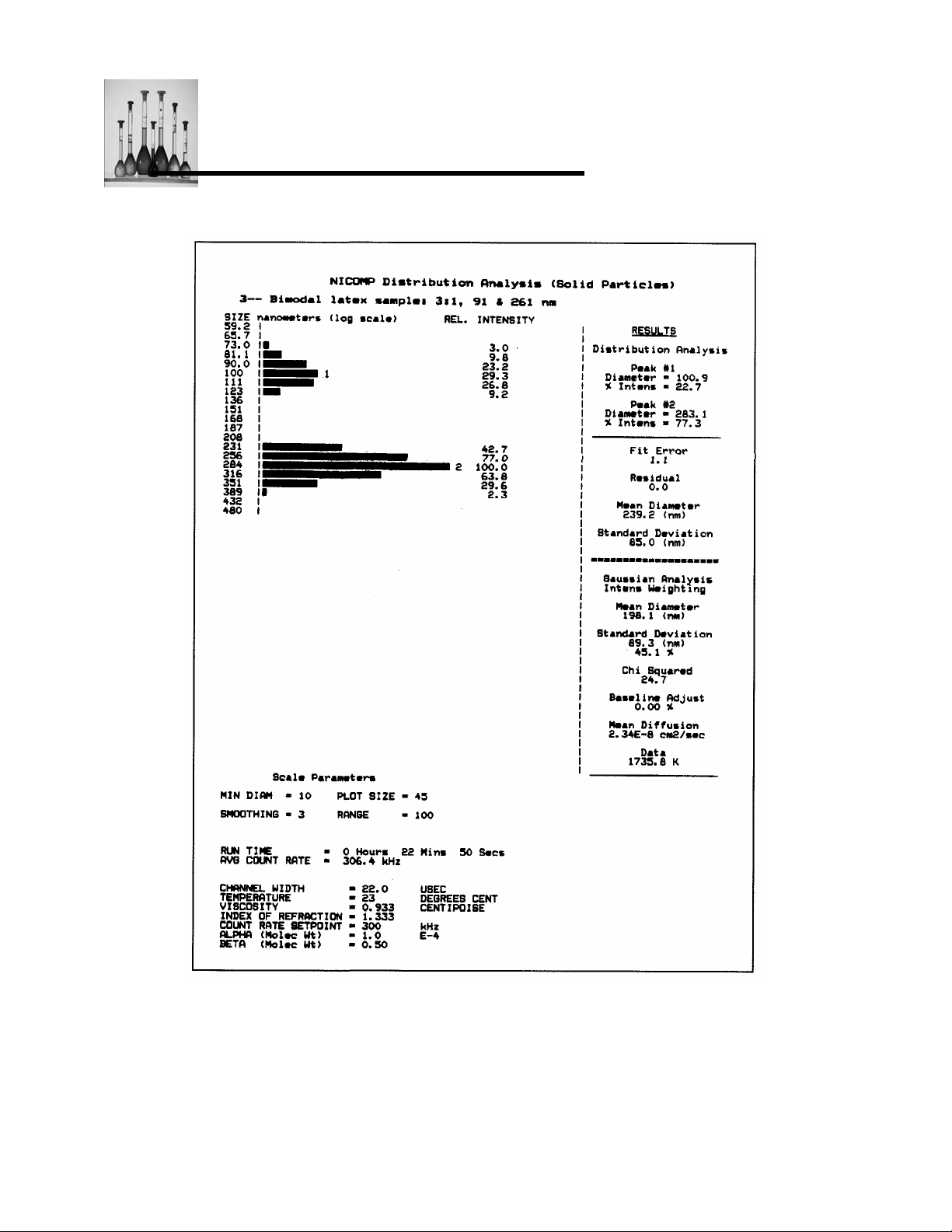
DDLLSS TThheeoorryy

Figure 19a Printout of the intensity-weighted Distribution Analysis result for the 3:1
91/261nm test bimodal

Nicomp 380 Manual
PSS-380Nicomp-030806
06/06
Page 2 - 64

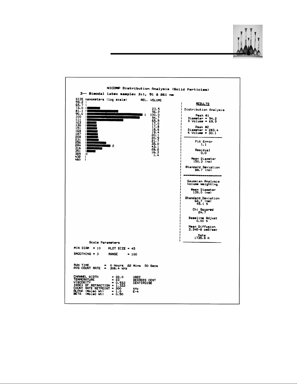
DDLLSS TThheeoorryy

Figure for the 19b: Printout of the volume-weighted Distribution Analysis result 91/261nm test
bimodal

Nicomp 380 Manual

PSS-380Nicomp-030806

06/06

Page 2 -65

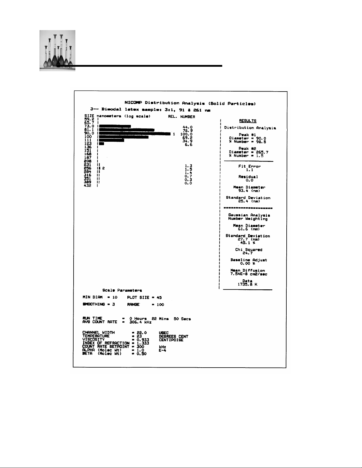
DDLLSS TThheeoorryy

Figure 19c: Printout of the number-weighted Distribution Analysis result for the
91/261 nm test bimodal

Nicomp 380 Manual
PSS-380Nicomp-030806
06/06
Page 2 - 66

DDLLSS TThheeoorryy

As mentioned above, we can generally conclude that the wider the separation of a bimodal, the

easier it is for the Distribution Analysis to perform an accurate measurement-again, provided

there is adequate scattering from the weakest of the two peaks. Figure 20 shows a logarithmic

plot of the reduced autocorrelation data for a 3:1 mixture (by mass, or volume) of 91 and 1091

nm latex standards. Here, for the first time, we see a very substantial curvature in the reduced
data, with the initial slope (at t’ =0) significantly greater than the final slope (at t’ = 64Δt’). This

difference notwithstanding, it is still surprising that there is no obvious “breakpoint” in the plot,

despite the factor-of-12 difference in the two constituent particle sizes. However, this sample is

handled with relative ease by the NICOMP algorithm. The Distribution Analysis result (video

display) is shown in Figure 21. After only 7 minutes of data acquisition, the analysis finds two

peaks, at 84 and 1041 nm, quite close to the correct values. Even the relative volumes are

accurate: 77/23%, compared to the ideal values of 75/25%.

In conclusion, it is worth returning to the issue of statistical accuracy of the autocorrelation

function and the stability of the results produced by the Distribution Analysis. Here, it turns out

to be even more important than for the Gaussian Analysis that adequate data be acquired so

that the ILT algorithm can settle to a reliable result. In general, the more complex the

distribution, the longer the time needed to obtain a stable result. This principle is illustrated

nicely by a sequence of results obtained from the 91/261 nm test bimodal discussed earlier.

This sample was run again, and a time sequence of volume-weighted printouts is shown in

Figure 22a-d, corresponding to run times of (approximately) 7 min., 10 min., 42 min. and 8

hours 10 min.

Nicomp 380 Manual

PSS-380Nicomp-030806

06/06

Page 2 -67

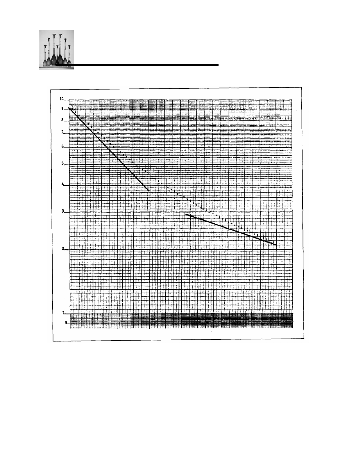
DDLLSS TThheeoorryy

Figure 20: Log
ratio, 91 and 1091 nm

Nicomp 380 Manual
PSS-380Nicomp-030806
06/06
Page 2 - 68

( C(t’)-B) vs. t’ for a widely-separated bimodal latex sample: 3:1 (vol.)

e

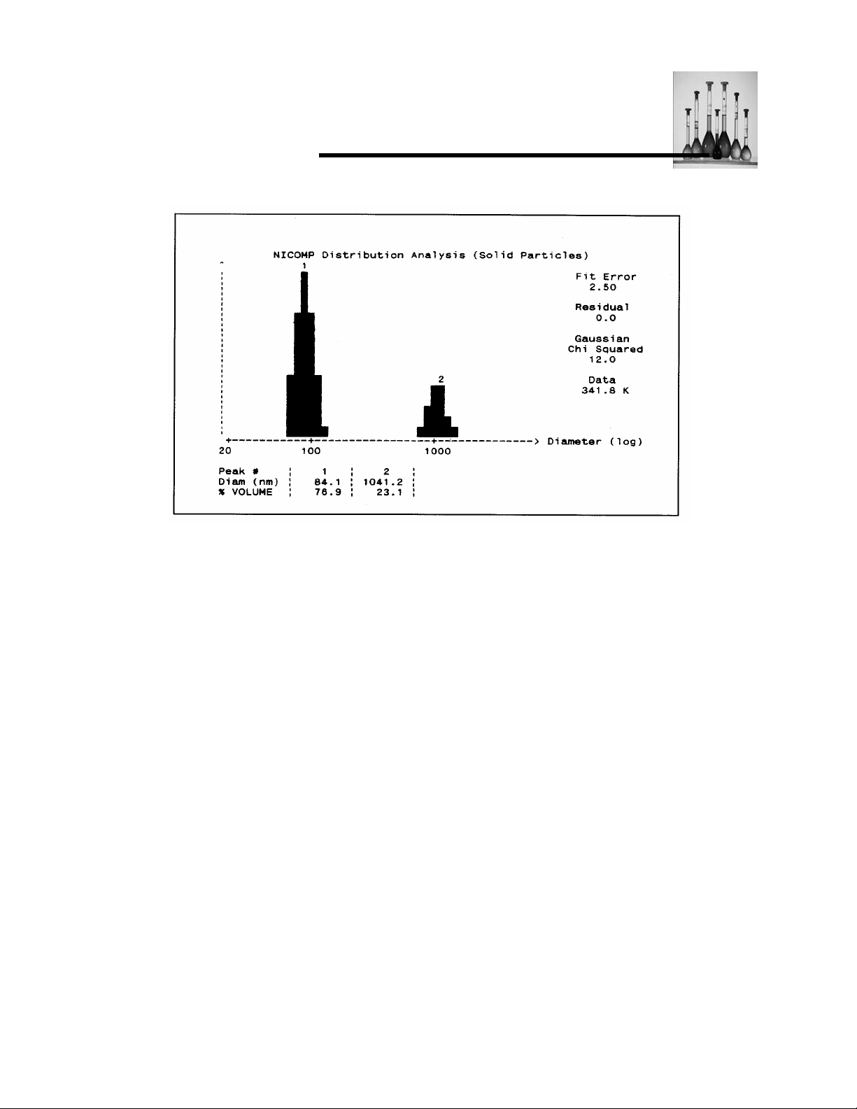
DDLLSS TThheeoorryy

Figure 21: The volume-weighted Distribution Analysis result for the 91/1091 sample
(Figure 20) nm bimodal

For this particular sample preparation, we see that the first two results agree very closely with

the known situation -- indeed, more closely than could normally be expected for these short data

acquisition times. After an elapsed time of 42 minutes (Figure 22c) the results have actually

degraded somewhat, although the peak mean diameter values are still within a few percent of

the correct answers. At this point the Fit Error has fallen to 1.0, with an ideal Residual of 0.0,

which easily fits our criteria of a finished run. When we return 8 hours later (Figure 22d), we find

a nearly perfect result, as regards both particle diameter and % volume for the two peaks.

Nicomp 380 Manual

PSS-380Nicomp-030806

06/06

Page 2 -69

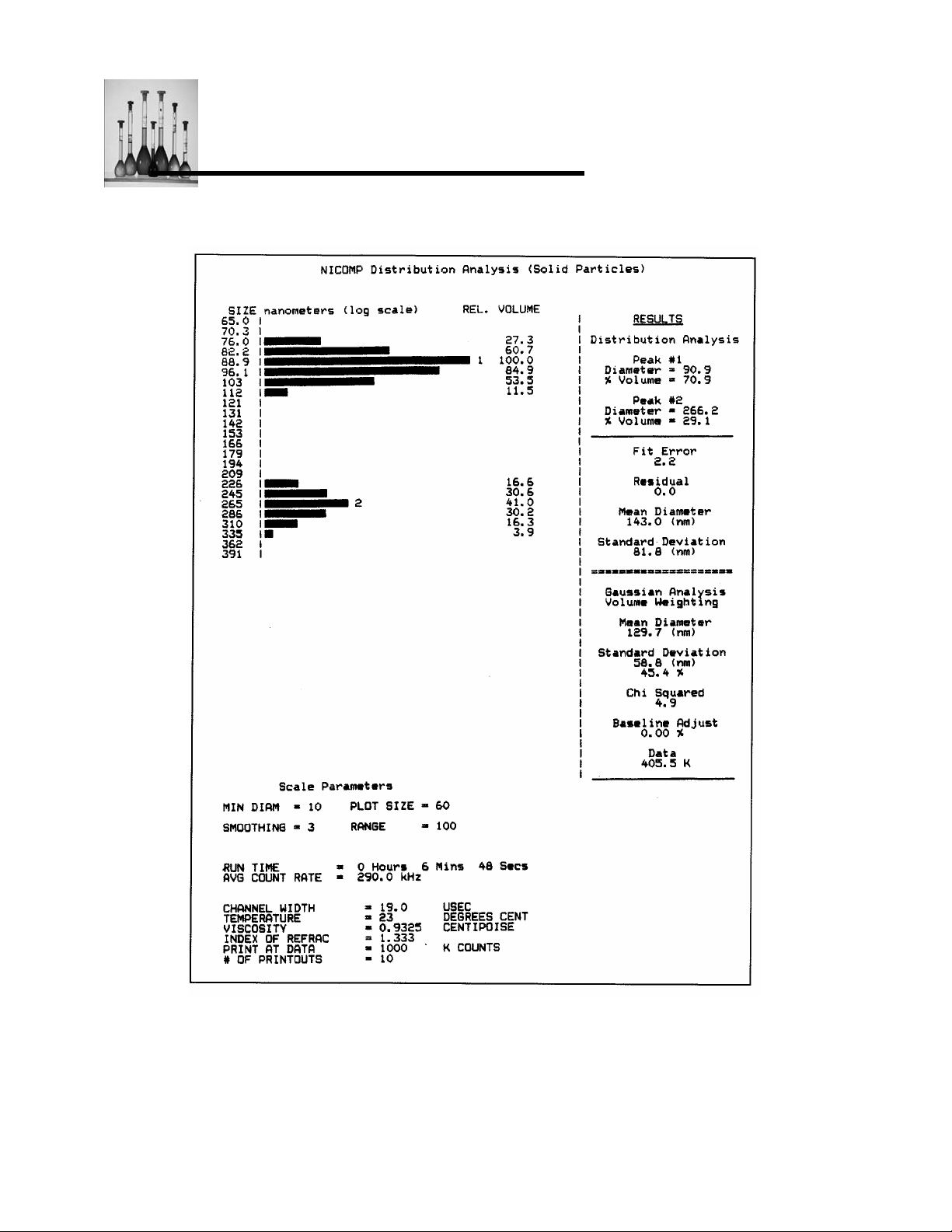
DDLLSS TThheeoorryy

Figure 22a: Printout of volume-weighted Distribution Analysis result for the 3:1
91/261 bimodal sample after 7 min

Nicomp 380 Manual
PSS-380Nicomp-030806
06/06
Page 2 - 70

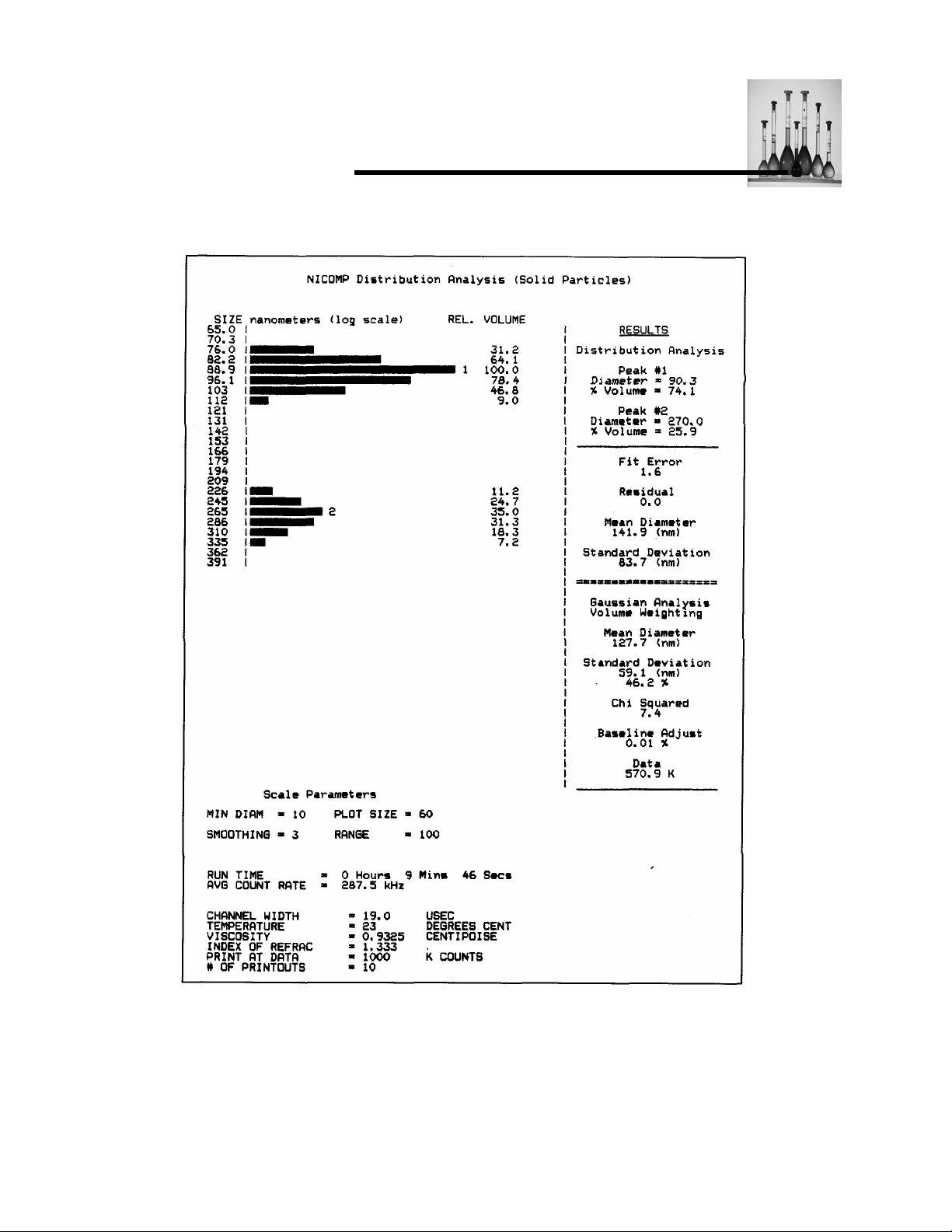
DDLLSS TThheeoorryy

Figure 22b: Printout of volume-weighted Distribution Analysis result for the 3:1
91/261 bimodal sample -- after 10 min

Nicomp 380 Manual

PSS-380Nicomp-030806

06/06

Page 2 -71

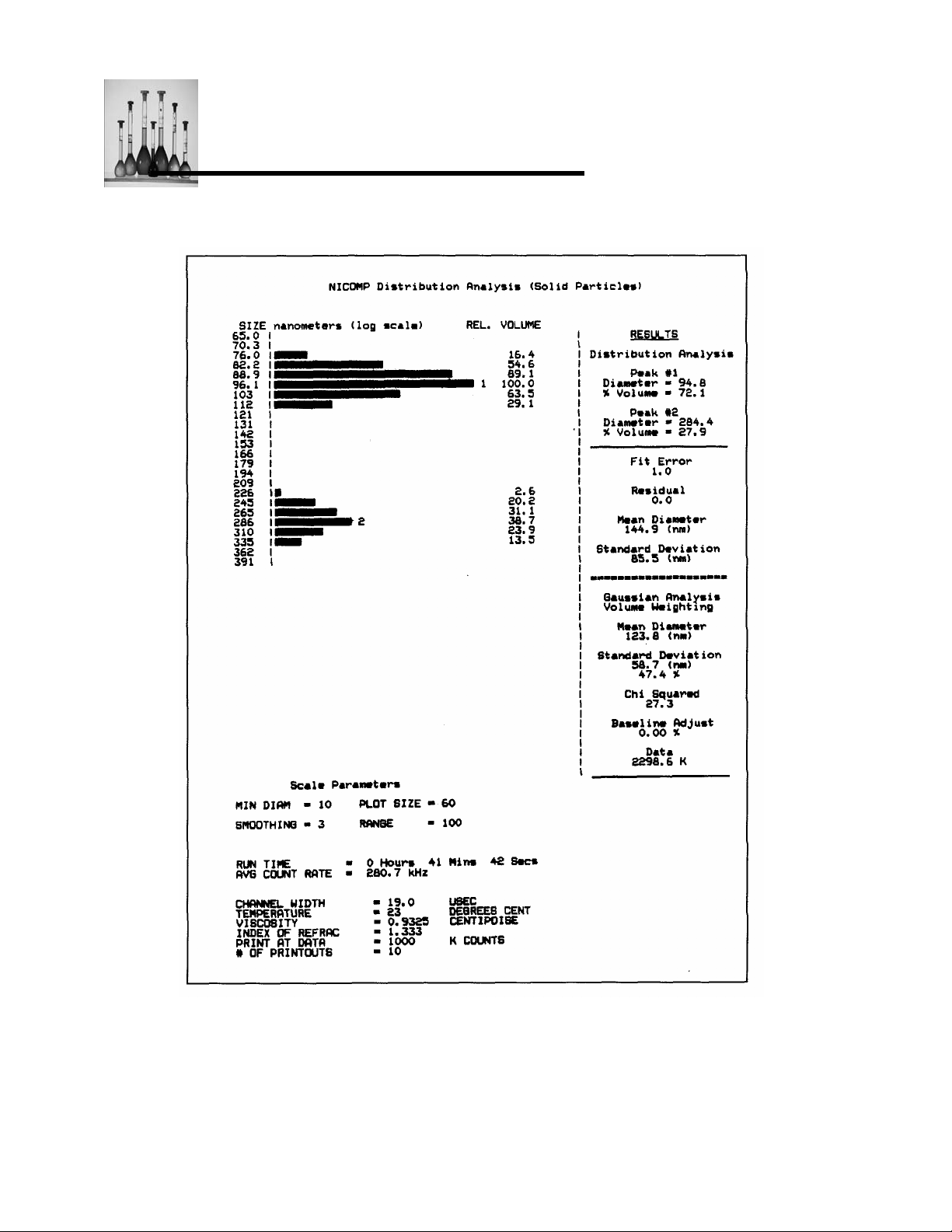
DDLLSS TThheeoorryy

Figure 22c: Printout of volume-weighted Distribution Analysis result for the 3:1 91/261
bimodal sample -- after 42 min

Nicomp 380 Manual
PSS-380Nicomp-030806
06/06
Page 2 - 72

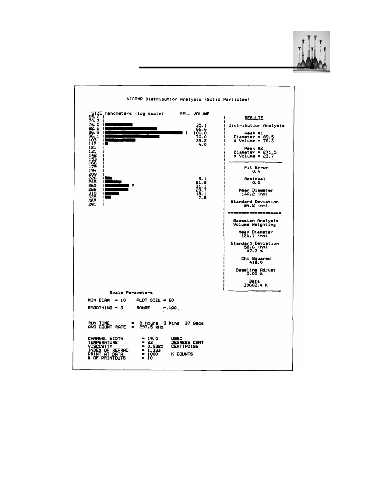
DDLLSS TThheeoorryy

Figure 22d: Printout of volume-weighted Distribution Analysis result for the 3:1
91/261 bimodal sample -- after 8 hrs, 10 min

Nicomp 380 Manual

PSS-380Nicomp-030806

06/06

Page 2 -73

DDLLSS TThheeoorryy

What is the lesson behind these printouts -- should samples be run for 8 hours? Certainly not!
Rather, the point is that if one wishes to optimize the analytical capabilities of the instrument,
they should make it a habit to obtain several intermediate printouts within the first 20 or 30
minutes of a run to verify the settling and stability of the computed distribution. Only in this way
will confidence be instilled in the user that the Distribution Analysis results are close to the best
that can be obtained by the DLS Module, given practical constraints on the total amount of the
allotted time.

Nicomp 380 Manual
PSS-380Nicomp-030806
06/06
Page 2 - 74

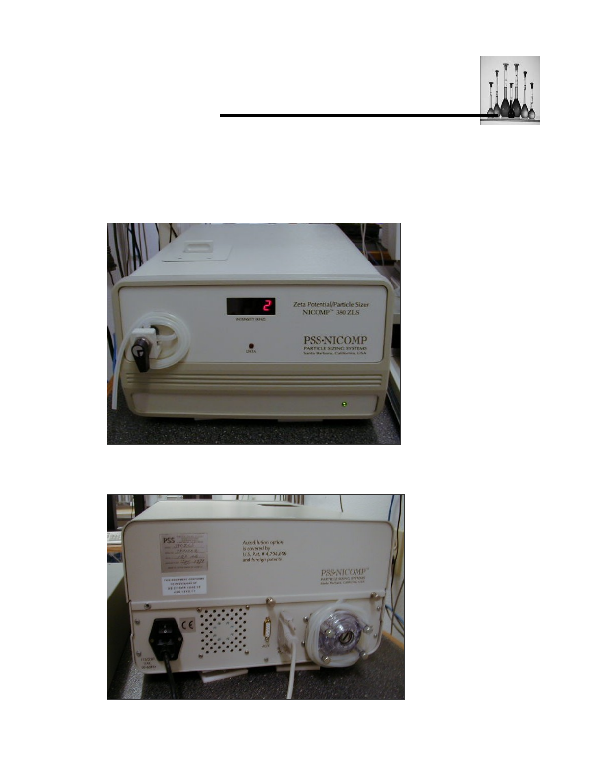
IInniittiiaall HHaarrddwwaarree SSeettuupp

INITIAL HARDWARE SETUP

1. Connect the 25-pin male connector of the cable provided to the port identified on the back of
the Nicomp instrument.

2. Connect the 9-pin female end of the connector to a serial port on the PC controller.

Nicomp 380 Manual

PSS-380Nicomp-030806

06/06

Page 3 - 1

IInniittiiaall HHaarrddwwaarree SSeettuupp

3. Plug the power cable provided into the back of the unit.

4. If the unit has the Autodilution feature, place the drain line into a waste bucket.

5. Apply power to the PC controller.

6. Install the Nicomp software package. Review the Software section of this manual.

7. Apply power to the Nicomp.

Nicomp 380 Manual
PSS-380Nicomp-030806
06/06
Page 3 - 2

SSooffttwwaarree IInnssttaallllaattiioonn

SOFTWARE INSTALLATION

The software program that is responsible for controlling the NICOMP Submicron Particle Sizer, and
also the NICOMP
when the program CW380 is run; it is displayed in the upper right-hand corner of the "default"
display screen, which is the Main Menu. The software diskette that is included with the NICOMP
380 will contain four software files:

CW388.EXE: the largest of the four files. It is the executable program which controls the
Instrument and initiates the running of the software.

CW388.CFG: contains the "configuration" of the 380 system. The configuration includes the
identification of the serial port for communication with the 380 instrument and the parallel port for
printing, as well as specification of available options, such as the flow pump for Autodilution, use
of an external laser and the multi-angle accessory. In some cases the CW380 CD Rom will be
missing the CW380.CFG file. This is not a mistake. Rather, after running and exiting the CW380
program, a CW380.CFG file will automatically be generated and stored in the disk drive and sub
directory which are specified in the Auto Print/Save Menu (Particle Sizing Window).

CW388.TBL: includes all of the information contained in the Auto Print/Save Menu and the
Control Menu (also accessed from the Particle Sizing Window). The former menu includes such
parameters as Data Storage Directory, Data File Name, Printout ID, Run Time, etc. The [F3]
Menu includes the following parameters, taken collectively, to define the conditions of data
collection,printout and storage:

 Autoset Channel Width  Liquid Viscosity
 Sample Temperature  Liquid Index of Refraction

In some cases a new CW388 software diskette that is sent will be missing the CW380.TBL file.
This is not a mistake. In the absence of this file, a default set of parameters will be used to define
The parameters in the two menus that are accessed by pressing the [F2] and [F3] Menu keys.
After the CW388 program is run and exited, a new CW388.TBL file will automatically be
generated and stored in the disk drive and sub-directory where the main CW388.EXE program is
located.

Generally it is recommended that the CW388 software files be copied to, and run from, the hard
disk drive. The software on the diskette can then be saved as a backup copy, to be reloaded in the
event of accidental erasure of a file or crash of the hard drive.

Computing Autocorrelator, is named CW388. The version # can be identified

Nicomp 380 Manual

PSS-380Nicomp-030806

06/06

Page 4 - 1

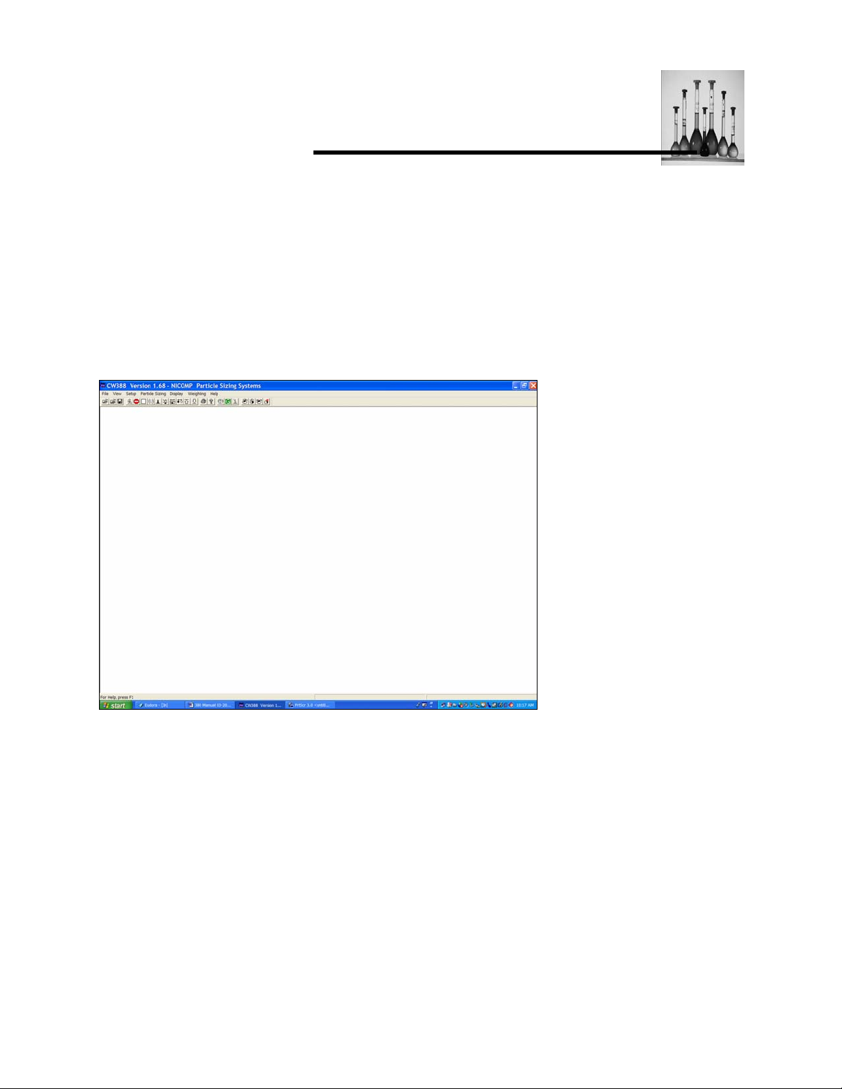
NNiiccoommpp SSooffttwwaarree

FILE

The following provides a brief summary of the File options that are used during the use of the
Windows CW388 Software

Access of the File options:

1. Position the highlight over the FILE option and click once using the mouse. The following
window of File options displays:

2. Position the highlight bar over the desired selection and click once. Following is a
description of each of the options offered.

Nicomp 380 Manual

PSS-380Nicomp-030806

06/06

Page 5 - 1

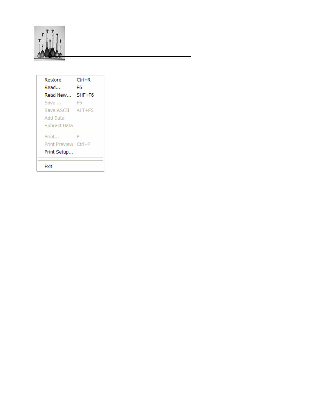
NNiiccoommpp SSooffttwwaarree

Restore

Used to restore collecting data once the autocorrelator has been halted.

Click on:

Yes: the screen will clear and data will be collected.
No: the warning screen will disappear and the autocorrelator will not start taking data.

Nicomp 380 Manual
PSS-380Nicomp-030806
06/06
Page 5 - 2

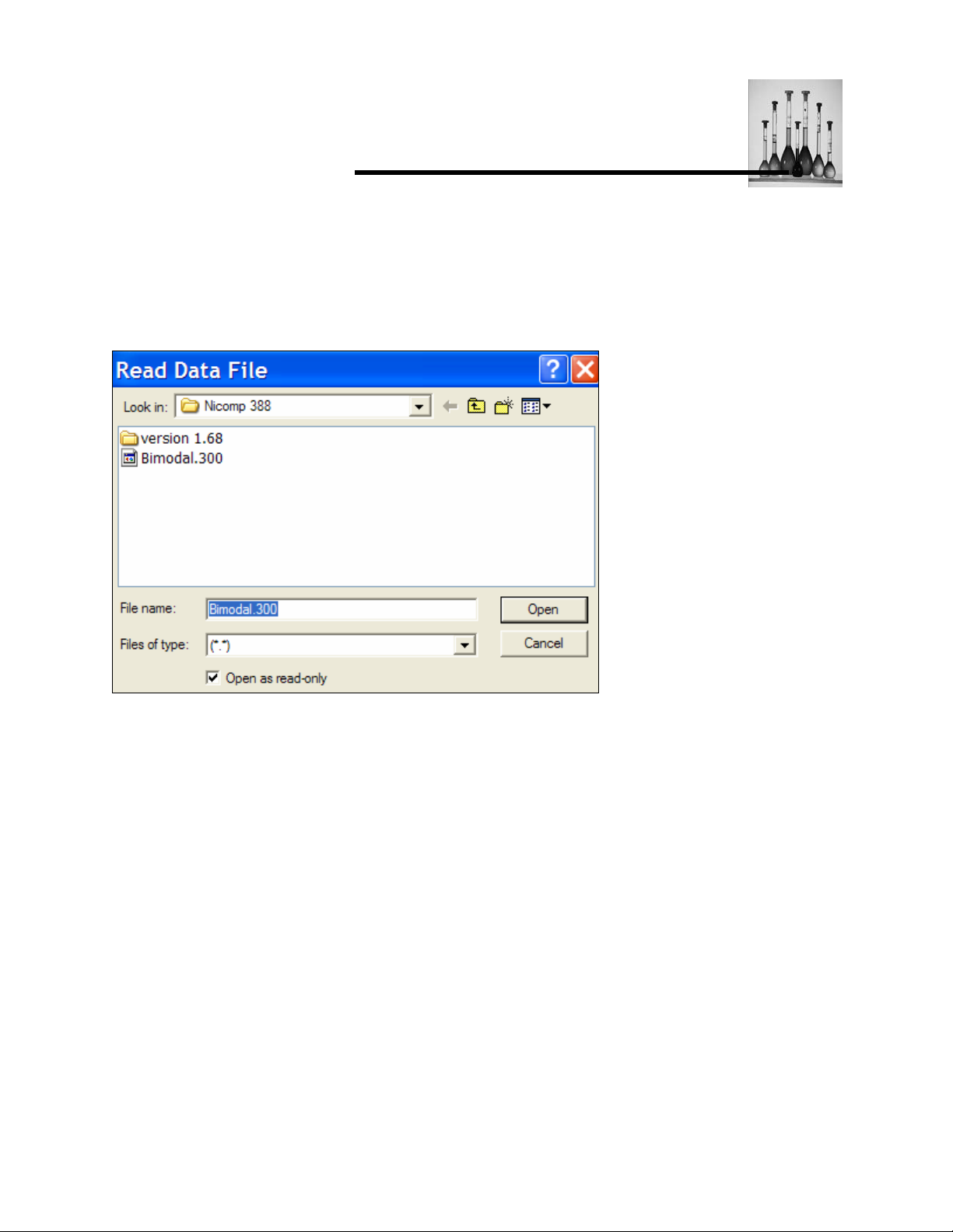
NNiiccoommpp SSooffttwwaarree

Read

A data file that has been stored following a measurement can be retrieved to display the
resulting particle size distribution (PSD), with the desired weighting. When this option is
selected, a list of data files will display in the Read Data File window such as in the example
below:

1. Position the highlight bar over the data file of interest and click the mouse once. Prior to the
selected data file being retrieved from memory, the following window will display:

2. Click on:

Yes: the data will be re-calculated.
No: the window will disappear and the volume-weighted distribution of the file selected

will display.

Nicomp 380 Manual

PSS-380Nicomp-030806

06/06

Page 5 - 3

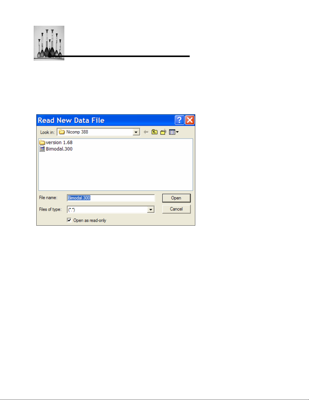
NNiiccoommpp SSooffttwwaarree

Read New

A data file that has been stored following a measurement can be retrieved to display the resulting
particle size distribution (PSD), with the desired weighting. When this option is selected, a list of
data files will display in the Read Data File window such as in the example below:

1. Position the highlight bar over the data file of interest and click the mouse.

2. Click on the OK button. The selected data file will be retrieved from memory. Once again the

CW388 Window for re-calculating the data will re-display. Please refer to the Read section of
this manual for additional information.

Nicomp 380 Manual
PSS-380Nicomp-030806
06/06
Page 5 - 4

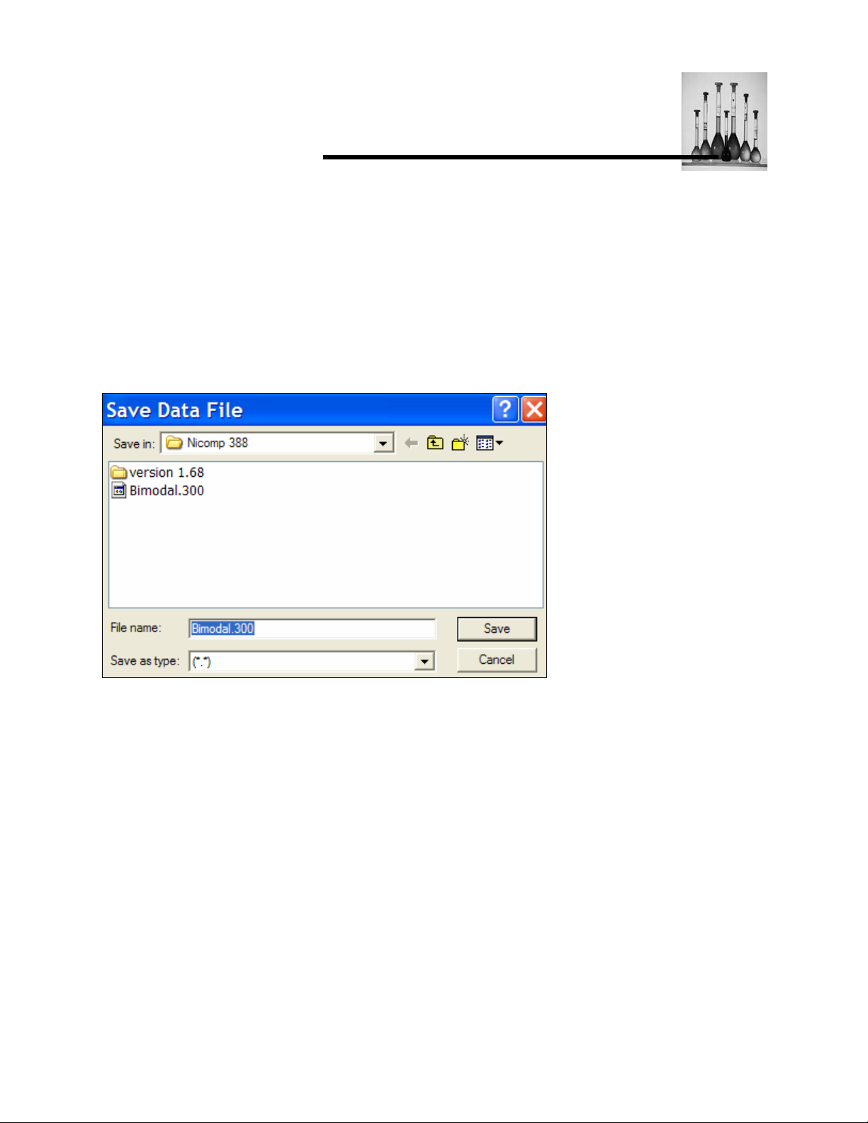
NNiiccoommpp SSooffttwwaarree

Save

This option is used throughout the CW388 software whenever a data file is to be saved. To access
this option:

1. Position the highlight bar over the File option and click the mouse once.

2. Position the highlight bar over the Save As option and click the mouse once. The following

screen will display:

Save ASCII

Use this option to save the data collected for a particular sample to an ASCII file format. The data
can then be imported to a spreadsheet program for presentation.

To create new files in standard ASCII format to export data files into other software packages (e.g.
spreadsheets), for manipulation of the original data follow these steps:

1. Select a data file.

2. Position the highlight bar over the File option and click once.

3. Position the highlight bar over the Save ASCII File option using the mouse and click once

the following window displays:

Nicomp 380 Manual

PSS-380Nicomp-030806

06/06

Page 5 - 5

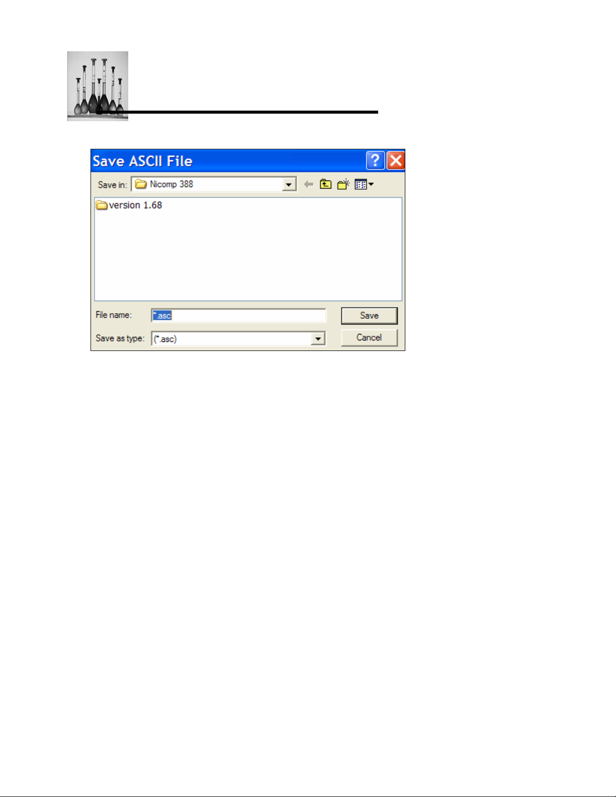
NNiiccoommpp SSooffttwwaarree

1. Type in the desired file name. A new file in ASCII format will be created and stored in the

Data Directory with the file extension .asc. If the same file name already exists, the

following message will appear:

2. Click on:

Yes: the existing ASCII file having the same file name will be erased, and the
new one stored in its place.
No: no new file will be stored.

Add Data

Subtract Data

Nicomp 380 Manual
PSS-380Nicomp-030806
06/06
Page 5 - 6