

Page 1

MapleSim User's Guide
Copyright © Maplesoft, a division of Waterloo Maple Inc.
2008-2010
Page 2

MapleSim User's Guide
Copyright
Maplesoft, MapleSim, and Maple are all trademarks of Waterloo Maple Inc.
© Maplesoft, a division of Waterloo Maple Inc. 2001-2010. All rights reserved.
No part of this book may be reproduced, stored in a retrieval system, ortranscribed, in any form or by anymeans
— electronic,mechanical, photocopying,recording,or otherwise.Informationin thisdocumentis subjecttochange
without notice and does not represent a commitment on the part of the vendor. The software described in this
document isfurnished underalicense agreementandmay beusedor copiedonlyin accordancewiththe agreement.
It is against the law to copy the software on any medium except as specically allowed in the agreement.
Java and all Java-based marks are trademarks or registered trademarks of Sun Microsystems, Inc. in the United
States and other countries. Maplesoft is independent of Sun Microsystems, Inc.
Linux is a registered trademark of Linus Torvalds.
Macintosh is a trademark of Apple Inc., registered in the U.S. and other countries.
Microsoft, Excel, and Windows are registered trademarks of Microsoft Corporation.
Modelica is a registered trademark of the Modelica Association.
All other trademarks are the property of their respective owners.
This document was produced using a special version of Maple and DocBook.
Printed in Canada
ISBN 978-1-897310-90-8
Page 3

Contents
Introduction .................................................................................................. vii
1 Getting Started with MapleSim ........................................................................ 1
1.1 Physical Modeling in MapleSim ................................................................ 1
Acausal and Causal Modeling ................................................................... 2
1.2 The MapleSim Window ........................................................................... 5
1.3 Basic Tutorial: Modeling an RLC Circuit and DC Motor ................................ 7
Building an RLC Circuit Model .................................................................. 7
Specifying Component Properties ............................................................. 11
Adding a Probe ..................................................................................... 11
Simulating the RLC Circuit Model ............................................................ 12
Building a Simple DC Motor Model .......................................................... 13
Simulating the DC Motor Model ............................................................... 15
2 Building a Model ........................................................................................ 17
2.1 The MapleSim Component Library .......................................................... 17
Viewing Help Topics for Components ........................................................ 18
2.2 Browsing a Model ................................................................................ 18
Model Tree ........................................................................................... 18
Model Navigation Controls ...................................................................... 19
2.3 Dening How Components Interact in a System ......................................... 20
2.4 Specifying Component Properties ............................................................ 21
Specifying Parameter Units ...................................................................... 21
Specifying Initial Conditions ................................................................... 22
2.5 Creating and Managing Subsystems ......................................................... 23
Example: Creating a Subsystem ................................................................ 23
Viewing the Contents of a Subsystem ........................................................ 25
Adding Multiple Copies of a Subsystem to a Model ...................................... 26
Editing Subsystem Denitions and Shared Subsystems ................................. 28
Working with Stand-alone Subsystems ....................................................... 32
2.6 Global and Subsystem Parameters ............................................................ 34
Global Parameters .................................................................................. 34
Subsystem Parameters ............................................................................ 36
Creating Parameter Blocks ...................................................................... 38
2.7 Attaching Files to a Model ...................................................................... 42
2.8 Creating and Managing Custom Libraries .................................................. 43
Example: Adding Subsystems and Attachments to a Custom Library ............... 43
2.9 Annotating a Model ............................................................................... 45
Example: Adding a Text Annotation to a Model ........................................... 46
2.10 Entering Text in 2-D Math Notation ........................................................ 47
2.11 Creating a Data Set for an Interpolation Table Component ........................... 48
Example: Creating a Data Set in Maple ...................................................... 48
2.12 Best Practices: Building a Model ........................................................... 49
iii
Page 4

iv • Contents
Best Practices: Laying Out and Creating Subsystems .................................... 49
Best Practices: Building Electrical Models .................................................. 50
Best Practices: Building 1-D Translational Models ....................................... 52
Best Practices: Building Multibody Models ................................................. 53
Best Practices: Building Hydraulic Models ................................................. 53
3 Creating Custom Modeling Components .......................................................... 55
3.1 Overview ............................................................................................ 55
3.2 Opening Custom Component Examples .................................................... 56
3.3 Example: Nonlinear Spring-Damper Component ......................................... 56
Opening the Custom Component Template ................................................. 58
Dening the Component Name and Equations ............................................. 58
Dening Component Ports ....................................................................... 59
Generating the Custom Component ........................................................... 60
3.4 Working with Custom Components in MapleSim ........................................ 61
3.5 Editing a Custom Component .................................................................. 62
4 Simulating and Visualizing a Model ................................................................ 63
4.1 How MapleSim Simulates a Model .......................................................... 63
4.2 Simulating a Model .............................................................................. 66
Simulation Parameters ............................................................................ 66
Editing Probe Values .............................................................................. 70
Storing Parameter Sets to Compare Simulation Results ................................. 70
4.3 Simulation Progress Messages ................................................................. 71
4.4 Managing Simulation Results ................................................................. 71
4.5 Customizing Plot Windows .................................................................... 72
Example: Plotting Multiple Quantities in Individual Graphs ........................... 73
Example: Plotting One Quantity Versus Another ......................................... 76
4.6 Plot Window Toolbar and Menus ............................................................. 78
4.7 Visualizing a Multibody Model ................................................................ 78
The 3-D Workspace ................................................................................ 79
Viewing and Browsing 3-D Models ........................................................... 80
Adding Shapes to a 3-D Model ................................................................. 81
Building a Model in the 3-D Workspace ..................................................... 85
Example: Building a Double Pendulum Model in the 3-D Workspace ............... 88
4.8 Best Practices: Simulating and Visualizing a Model .................................... 96
5 Analyzing and Manipulating a Model ............................................................. 97
5.1 Overview ............................................................................................ 97
5.2 Retrieving Equations and Properties from a Model ..................................... 99
5.3 Analyzing Linear Systems .................................................................... 100
5.4 Optimizing Parameters ......................................................................... 101
5.5 Generating C Code from a Model ........................................................... 102
5.6 Working with Maple Embedded Components ........................................... 103
6 MapleSim Tutorials .................................................................................... 105
6.1 Tutorial 1: Modeling a DC Motor with a Gearbox ...................................... 105
Page 5

Contents • v
Adding a Gearbox to a DC Motor Model .................................................. 105
Simulating the DC Motor with Gearbox Model .......................................... 106
Grouping the DC Motor Components into a Subsystem ............................... 107
Assigning Global Parameters to a Model ................................................... 108
Changing Input and Output Values .......................................................... 109
6.2 Tutorial 2: Modeling a Cable Tension Controller ....................................... 111
Building a Cable Tension Controller Model ............................................... 111
Specifying Component Properties ............................................................ 113
Simulating the Cable Tension Controller ................................................... 113
6.3 Tutorial 3: Modeling a Nonlinear Damper ................................................ 114
Generating a Custom Spring Damper ....................................................... 114
Providing Damping Coefcient Values ..................................................... 115
Building the Nonlinear Damper Model .................................................... 116
Assigning a Parameter to a Subsystem ..................................................... 118
Simulating the Nonlinear Damper with Linear Spring Model ........................ 119
6.4 Tutorial 4: Modeling a Planar Slider-Crank Mechanism .............................. 120
Creating a Planar Link Subsystem ........................................................... 121
Dening and Assigning Parameters ......................................................... 124
Creating the Crank and Connecting Rod Elements ...................................... 124
Adding the Fixed Frame, Sliding Mass, and Joint Elements .......................... 125
Specifying Initial Conditions .................................................................. 126
Simulating the Planar Slider-Crank Mechanism .......................................... 126
7 Reference: MapleSim Keyboard Shortcuts ...................................................... 129
Glossary ..................................................................................................... 131
Index ......................................................................................................... 133
Page 6

vi • Contents
Page 7

Introduction
MapleSim Overview
MapleSimTMis amodeling environment forcreating andsimulating complexmulti-domain
physical systems.It allowsyou tobuild component diagrams that represent physical systems
in a graphicalform. Usingboth symbolic andnumeric approaches,MapleSim automatically
generates model equations from a component diagram and runs high-delity simulations.
Build Complex Multi-domain Models
You can use MapleSimto buildmodels thatintegrate componentsfrom variousengineering
elds intoa completesystem. MapleSimfeatures alibrary ofover 300modeling components,
including electrical, hydraulic, mechanical, and thermal devices; sensors and sources; and
signal blocks.You can also createcustom componentsto suityour modelingand simulation
needs.
Advanced Symbolic and Numeric Capabilities
MapleSim uses the advanced symbolic and numeric capabilities of MapleTMto generate
the mathematicalmodels thatsimulate thebehavior ofa physical system. Youcan, therefore,
apply simplication techniques to equations to create concise and numerically efcient
models.
Pre-built Analysis Tools and Templates
MapleSim providesvarious pre-builttemplates inthe formof Mapleworksheets for viewing
model equations and performing advanced analysis tasks, such as parameter optimization.
To analyze your model and present your simulation results in an interactive format, you
can useMaple featuressuch asembedded components,plotting tools,and documentcreation
tools. You can also translate your models into C code and work with them in other applications and tools, including applications that allow you to perform real-time simulation.
Interactive 3-D Visualization Tools
The MapleSim 3-D visualization environment allows you to build and animate 3-D graphical representations of your multibody mechanical system models. You can use this environment to validate the 3-D conguration of your model and visually analyze the behavior
of your system under different conditions.
vii
Page 8
viii • Introduction
Related Products
MapleSim requires the latest version of Maple 14.
MaplesoftTMalso offers a suite of toolboxes, add-ons, and other applications that extend
the capabilities of Maple and MapleSim for engineering design projects.
For a complete list of products, visit http://www.maplesoft.com/products.
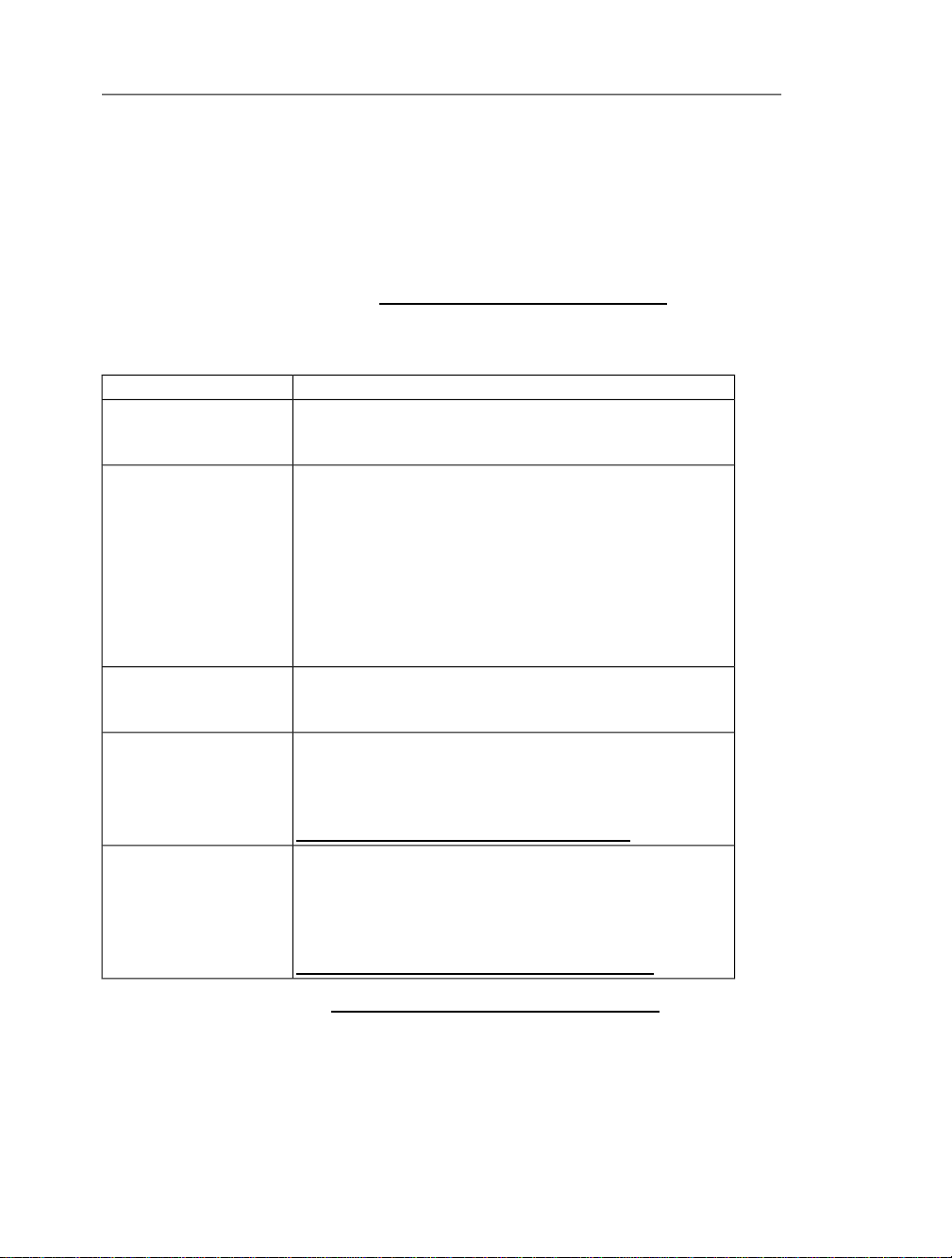
Related Resources
DescriptionResource
MapleSim Installation
Guide
MapleSim Help System
System requirements and installation instructionsfor MapleSim.
The MapleSimInstallation Guide is available inthe Install.html
le on your MapleSim installation DVD.
Provides the following information:
• MapleSim User's Guide: conceptual information about
MapleSim, an overview of MapleSim features, and tutorials
to help you get started.
• Using MapleSim: help topics for model building, simulation,
and analysis tasks.
• MapleSim Library Reference Guide: descriptions of the
modeling components available in MapleSim.
Sample modelsfrom variousengineering domains. Thesemodels
MapleSim Examples
MapleSim Online Resources
MapleSim Application
Center
are available in the Examples palette in theLibraries tab on the
left side of the MapleSim window.
Training webinars, product demonstrations, videos, sample applications, and more.
For more information, visit
http://www.maplesoft.com/products/maplesim.
A collectionofsample models,customcomponents, andanalysis
templates that youcan download anduse in your MapleSimprojects.
For more information, visit
http://www.maplesoft.com/applications/maplesim.
For additional resources, visit http://www.maplesoft.com/site_resources.
Page 9

Introduction • ix
Getting Help
To requestcustomer supportor technicalsupport, visithttp://www.maplesoft.com/support.
Customer Feedback
Maplesoft welcomes your feedback. For comments related to the MapleSim product documentation, contact doc@maplesoft.com.
Page 10

x • Introduction
Page 11

1 Getting Started with MapleSim
In this chapter:
• Physical Modeling in MapleSim (page 1)
• The MapleSim Window (page 5)
• Basic Tutorial: Modeling an RLC Circuit and DC Motor (page 7)
1.1 Physical Modeling in MapleSim
Physical modeling,or physics-basedmodeling, incorporatesmathematics andphysical laws
to describe the behavior of an engineering component or a system of interconnected components. Sincemost engineeringsystems haveassociated dynamics,the behavioris typically
dened with ordinary differential equations (ODEs).
To help youdevelop models quicklyand easily, MapleSim providesthe following features:
Topological or “Acausal” System Representation
The signal-ow approach used by traditional modeling tools requires system inputs and
outputs to be dened explicitly. In contrast, MapleSim allows you to use a topological
representation to connect interrelated components without having to consider how signals
ow between them.
Mathematical Model Formulation and Simplification
A topological representation maps readily to its mathematical representation and the symbolic capability of MapleSim automates the generation of system equations.
When MapleSimformulates thesystem equations,several mathematicalsimplication tools
are applied to remove any redundant equations and multiplication by zero or one.The simplication tools then combine and reduce the expressions to get a minimal set of equations
required to represent a system without losing delity.
Advanced Differential Algebraic Equation Solvers
Algebraic constraints areintroduced in the topologicalapproach to model denition.Problems that combine ODEs with these algebraic constraints are called Differential Algebraic
Equations (DAEs).Depending onthe natureof theseconstraints, the complexity of the DAE
problem can vary. An index of the DAEs provides a measure of the complexity of the
problem. Complexity increases with the index of the DAEs.
The development ofgeneralized solvers for complex DAEs is the subject of much research
in the symbolic computation eld. With Maple as its computation engine, MapleSim uses
1
Page 12
2 • 1 Getting Started with MapleSim
advanced DAE solvers that incorporate leading-edge symbolic and numeric techniques for
solving high-index DAEs.
Acausal and Causal Modeling
Real engineered assemblies, such as motors and powertrains, consist of a network of interacting physical components. They are commonly modeled in software by block diagrams.
The lines connecting two blocks indicate that they are coupled by physical laws.
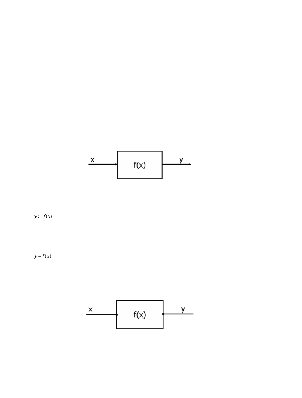
When simulatedby software,block diagramscan eitherbe causalor acausal.Many simulation
tools arerestricted tocausal (or signal-ow) modeling. Inthese tools,a unidirectionalsignal,
which is essentially a time-varying number, ows into a block. The block then performs a
well-dened mathematicaloperation on the signal andthe resultows out of the otherside.
This approach is useful for modeling systems that are dened purely by signals that ow
in a single direction, such as control systems and digital lters.
This approach isanalogous to an assignment,where a calculation isperformed on a known
variable orset ofvariables on the right handside andthe result is assigned toanother variable
on the left:
Modeling how real physical components interact requires a different approach. In acausal
modeling, a signalfrom two connected blocks travels in both directions. The programming
analogy would be a simple equality statement:
The signalincludes informationabout whichphysical quantities(for example,energy, current,
torque, heat and mass ows) must be conserved. The blocks contain information about
which physical laws(represented by equations) they must obey and, hence, which physical
quantities must be conserved.
Page 13
1.1 Physical Modeling in MapleSim • 3
MapleSim allows you to use both approaches. You can simulate a physical system (with
acausal modeling)together with the associated logic or controlloop (with causal modeling)
in a manner that suits either task best.
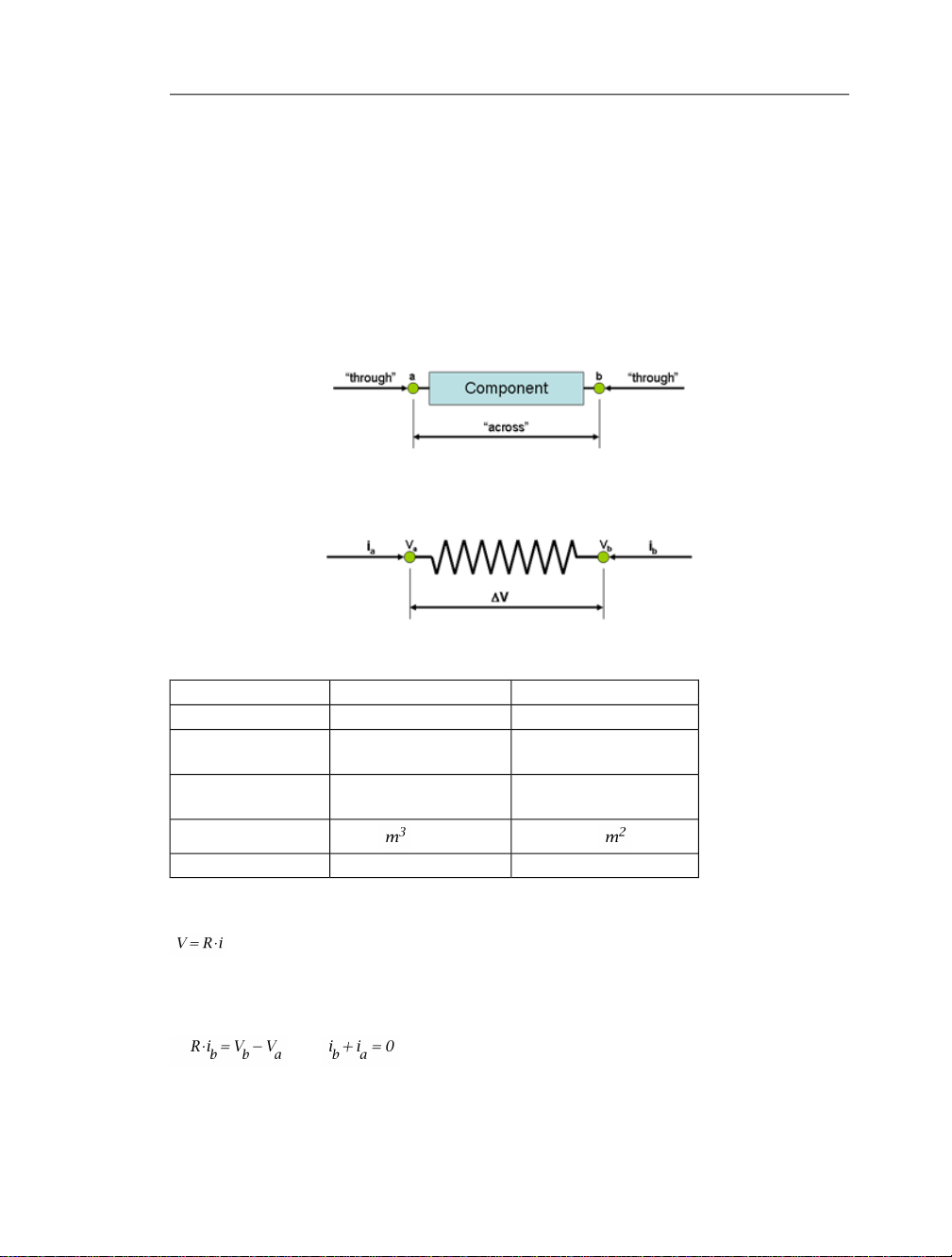
Through and Across Variables
When using the acausal modeling approach, it is useful to identify the through and across
variables ofthe componentyou aremodeling. In general terms, anacross variablerepresents
the driving force in a system and a through variable represents the ow of a conserved
quantity:
For example, in an electrical circuit, the through variable, i, is the current and the across
variable, V, is the voltage drop:
The following table lists some examples of through and across variablesfor other domains:
AcrossThroughDomain
Electrical
Mechanical (transla-
tional)
Mechanical (rotation-
al)
Hydraulic
Heat ow
Voltage (V)Current (A)
Velocity (m/s)Force (N)
Angular Velocity (rad/s)Torque (N.m)
Pressure (N/ )Flow ( /s)
Temperature (K)Heat ow (W)
As a simple example, the form of the governing equation for a resistor is
This equation,in conjunctionwith Kirchhoff’sconservation ofcurrent law,allows acomplete
representation of a circuit.
and
Page 14
4 • 1 Getting Started with MapleSim
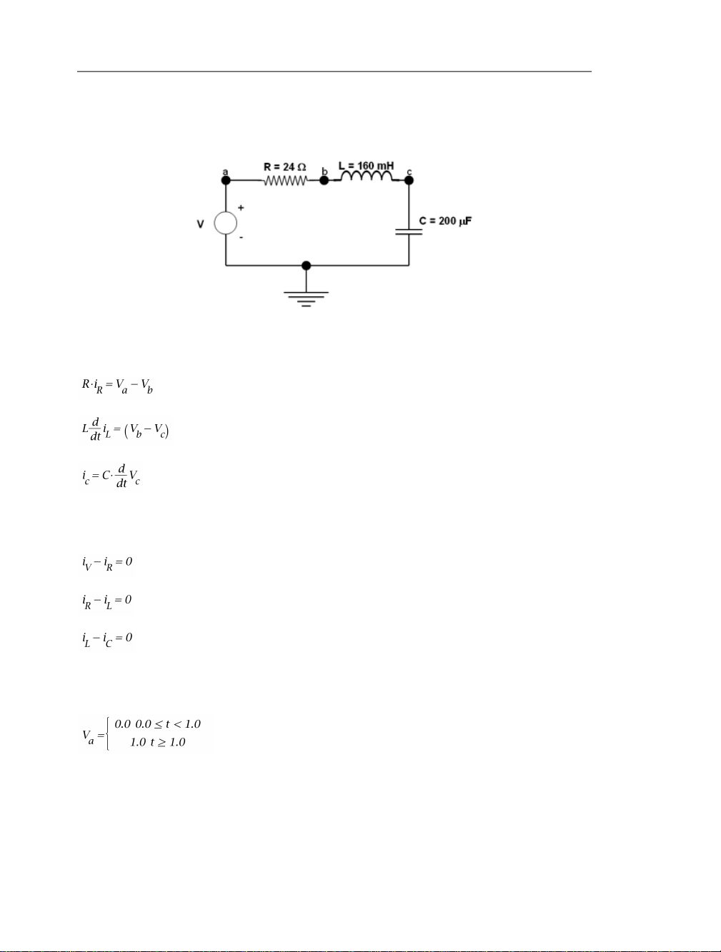
To extend this example, the following schematic diagram describes an RLC circuit, an
electrical circuit consisting of a resistor, inductor, and a capacitor connected in series:
If you wanted to model this circuit manually, it can be represented with the following
characteristic equations for the resistor, inductor, and capacitor respectively:
By applying Kirchhoff's current law, the following conservation equations are at points a,
b, and c:
These equations, along with a denition of the input voltage (dened as a transient going
from 0 to 1 volt, 1 second after the simulation starts)
provide enough information to dene the model and solve for the voltages and currents
through the circuit.
In MapleSim, all of these calculations are performed automatically; you only need to draw
the circuit and provide the component parameters. These principles can be applied equally
Page 15
1.2 The MapleSim Window • 5
to allengineering domainsin MapleSimand allowyou toconnect componentsin onedomain
with components in others easily.
In the Basic Tutorial: Modeling an RLC Circuit and DC Motor (page 7) section of this
chapter, you will model the RLC circuit described above. The following image shows how
the RLC circuit diagram appears when it is built in MapleSim.
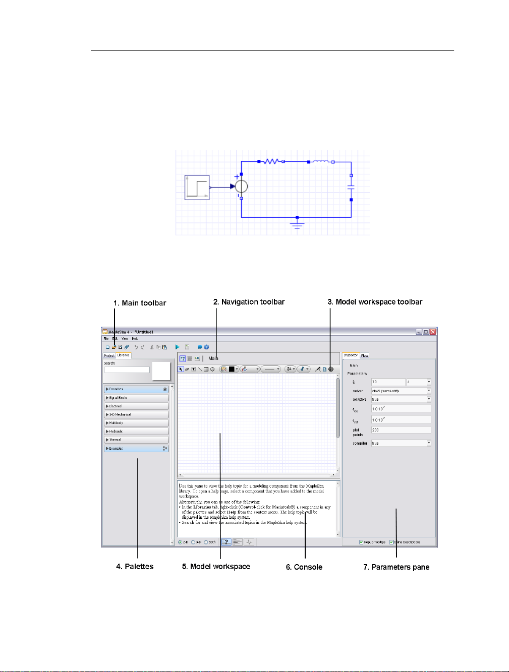
1.2 The MapleSim Window
In the default view, the MapleSim window contains the following panes and components:
Page 16
6 • 1 Getting Started with MapleSim
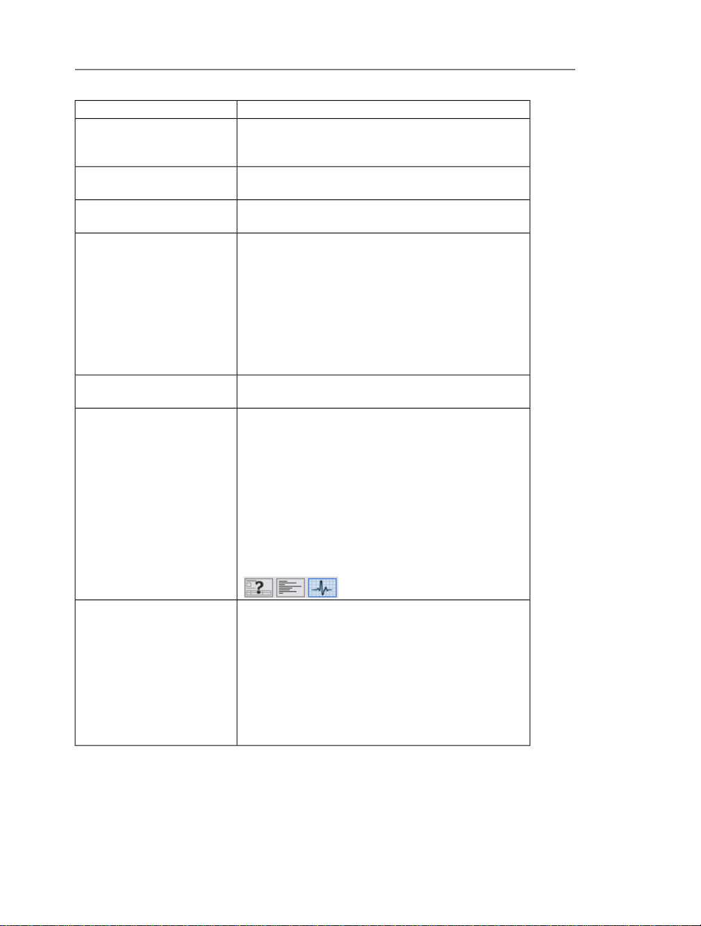
DescriptionComponent
Contains tools for running a simulation, attaching
1. Main toolbar
2. Navigation toolbar
3. Model workspace toolbar
4. Palettes pane
MapleSim analysistemplates toyour model, and performing other common tasks.
Contains tools for browsing your model and subsystems
hierarchically, and changing the model view.
Contains tools for laying out and selecting objects, and
adding elements such as annotations and probes.
Contains expandable menus withtools that you can use to
build a model and manage your MapleSim project. This
pane contains two tabs:
• Libraries tab: containspalettes withsample modelsand
domain-specic componentsthat youcanadd tomodels.
• Project tab: contains palettes with tools to help you
browse and build a model, and manage simulation results, probes, and documents that you attach to a model.
5. Model workspace
6. Console
7. Parameters pane
The area in which you build and edit a model in a block
diagram view.
Contains the following panes:
• Help pane: displays the help topic associated with a
modeling component.
• Message Console pane: displaysprogress messages in-
dicating the status of the MapleSim engine during a
simulation.
• Debugging pane: displays diagnostic messages as you
build your model.
You can use the buttons below the console
( ) to display each pane.
Contains the following tabs:
• Inspector tab: allows you to view and edit modeling
component properties, such as names and parameter
values, andspecify simulationoptions andprobe values.
• Plots tab: allowsyou todene customlayouts forsimu-
lation graphs and plot windows.
The contentsof thispane changedepending onyour selec-
tion in the model workspace.
MapleSim alsoprovides a3-D workspacethat youcan use to build, animate,and manipulate
3-D multibodymodels. Formore information,see Visualizinga Multibody Model (page 78)
in Chapter 4.
Page 17

1.3 Basic Tutorial: Modeling an RLC Circuit and DC Motor • 7
1.3 Basic Tutorial: Modeling an RLC Circuit and DC Motor
This tutorial introduces you to the modeling components and basic tools in MapleSim. It
illustrates the ability to mix causal models with acausal models.
In this tutorial, you will perform the following tasks:
1. Build an RLC circuit model.
2. Set parameter values to specify component properties.
3. Add probes to identify values of interest for the simulation.
4. Simulate the RLC circuit model.
5. Modify the RLC circuit diagram to create a simple DC motor model.
6. Simulate the DC motor model using different parameters.
Building an RLC Circuit Model
To buildthe RLC circuitdiagram, youadd componentsin the modelworkspace andconnect
them ina system.In this example, the RLCcircuit modelcontains ground,resistor, inductor,
capacitor, and signal voltage source components from the Electrical component library. It
also contains a step input source, which is a signal generator that drives the input voltage
level in the circuit.
Page 18
8 • 1 Getting Started with MapleSim
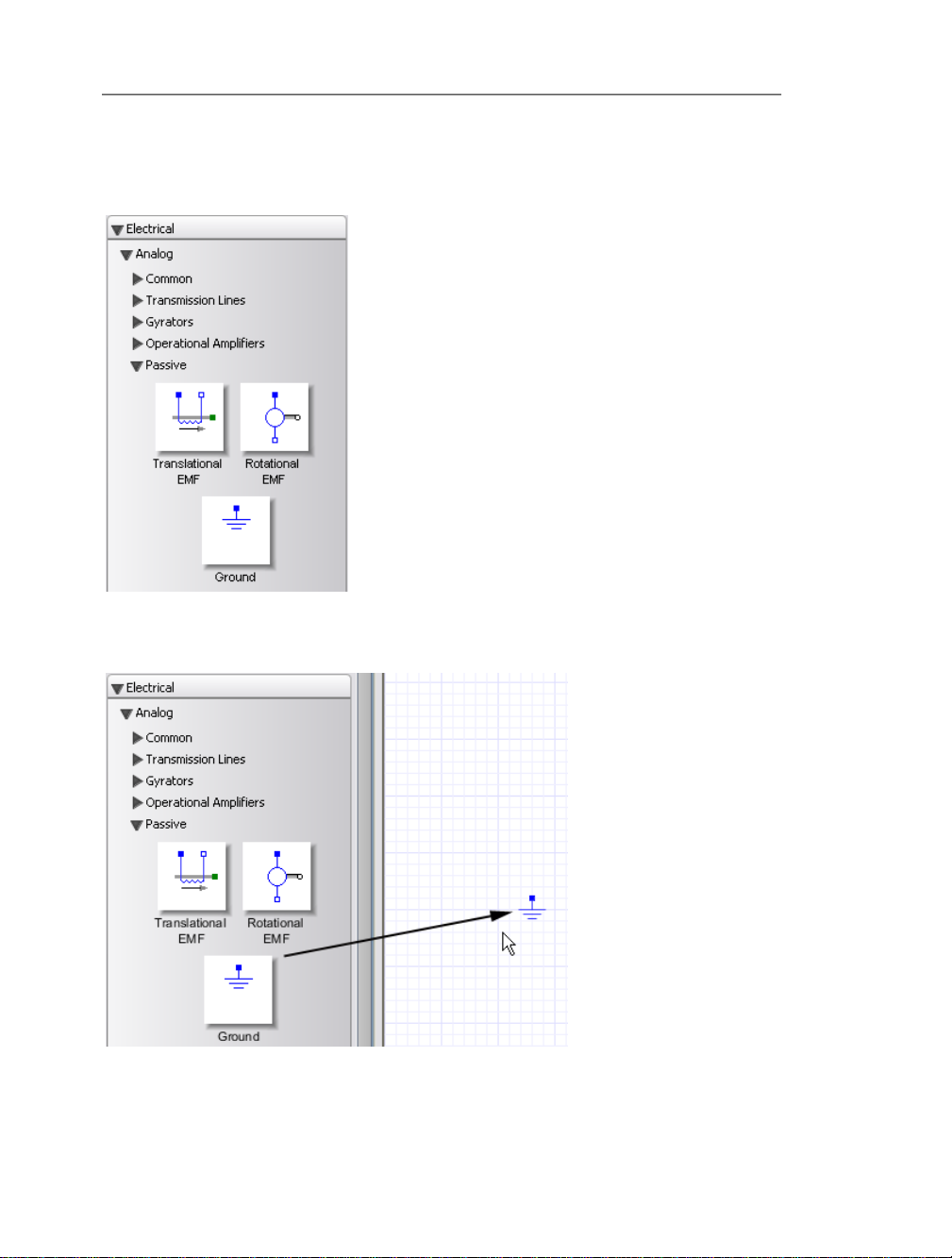
1. Inthe Librariestab at theleft ofthe modelworkspace, click the triangle besideElectrical
to expand the palette. In the same way, expand the Analog menu, and then expand the
Passive submenu.
2. From the Electrical → Analog → Passive menu, drag the Ground component to the
model workspace.
3. Add the remaining electrical components to the model workspace.
Page 19
1.3 Basic Tutorial: Modeling an RLC Circuit and DC Motor • 9
• From the Electrical → Analog → Passive→ Resistors menu, addthe Resistorcompon-
ent.
• From the Electrical → Analog → Passive → Inductors menu, add the Inductor com-
ponent.
• From the Electrical → Analog → Passive → Capacitors menu, add the Capacitor
component.
• From the Electrical → Analog → Sources → Voltage menu, add the Signal Voltage
component.
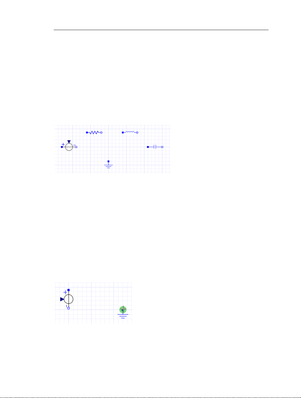
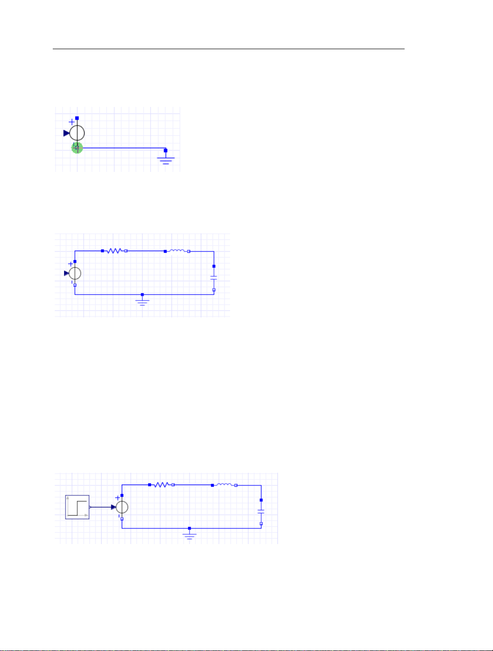
4. Drag the components in the arrangement shown below.
5. To rotate the Signal Voltage component clockwise, right-click (Control-click for
Macintosh®) the Signal Voltage component in the model workspace and select Rotate
Clockwise.
6. To ip the component horizontally, right-click (Control-click for Macintosh) the component again and select Flip Horizontal. Make sure that the positive (blue) port is at the
top.
7. Torotate theCapacitor component clockwise,right-click (Control-click forMacintosh)
the Capacitor icon in the model workspace and select Rotate Clockwise.
You can now connect the modeling components to dene interactions in your system.
8. Hover your mouse pointer over the Ground component port. The port is highlighted in
green.
Page 20
10 • 1 Getting Started with MapleSim
9. Click the Ground input port to start the connection line.
10. Hover your mouse pointer over the negative port of the Signal Voltage component.
11. Click the port once. The Ground component is connected to the Signal Voltage com-
ponent.
12. Connect the remaining components in the arrangement shown below.
You can now add a source to your model.
13. Expand theSignal Blocks palette. Expand theSources menu and then expand the Real
submenu.
14. From the palette, drag the Step source and place it to the left of the Signal Voltage
component in the model workspace.
The step source has a specic signal ow, which is represented by the arrows on the connections. This ow causes the circuit to respond to the input signal.
15. Connect the Step source to the Signal Voltage component. The complete RLC circuit
model is displayed below.
Page 21
1.3 Basic Tutorial: Modeling an RLC Circuit and DC Motor • 11
Specifying Component Properties
To specify component properties, you can set parameter values for components in your
model.
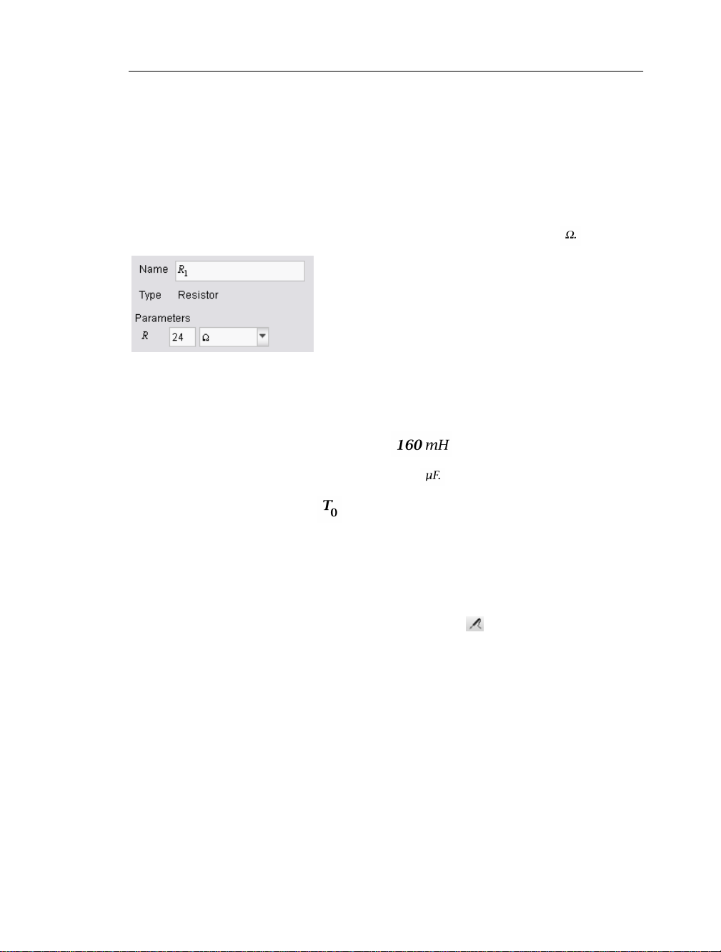
1. In the model workspace, click the Resistor component. The Inspector tab at the right of
the model workspace displays the name and parameter values of the resistor.
2. In the R eld, enter 24, and press Enter. The resistance is changed to 24
3. Specify the following parameter values for the other components. You can specify units
for a parameter by selecting a value from the drop-down menu found beside the parameter
value eld.
• For the Inductor, specify an inductance of .
• For the Capacitor, specify a capacitance of 200
• For the Step source, specify a value of 0.1 s.
Adding a Probe
To specify data values for a simulation, you must attach probes to lines or ports to the
model. In this example, you will measure the voltage of the RLC circuit.
1. In the model workspace toolbar, click the probe button ( ).
2. Hover your mouse pointer over the line that connects the Inductor and Capacitor
components. The line is highlighted.
3. Left-click the line once. The probe is displayed in the model workspace.
4. Drag the probe to position it and then click the probe once to place it on the line.
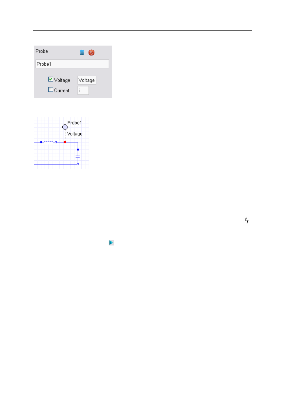
5. Select the probe. The probe properties are displayed in the Inspector tab at the right of
the model workspace.
6. Select the Voltage check box to include the voltage quantity in the simulation graph.
7. To display a custom name for this quantity in the model workspace, enter Voltage as
shown below and press Enter.
Page 22
12 • 1 Getting Started with MapleSim
The probe is added to the connection line.
Simulating the RLC Circuit Model
Before simulatingyour model,you canspecify theduration for which to run the simulation.
1. Click a blank area in the model workspace.
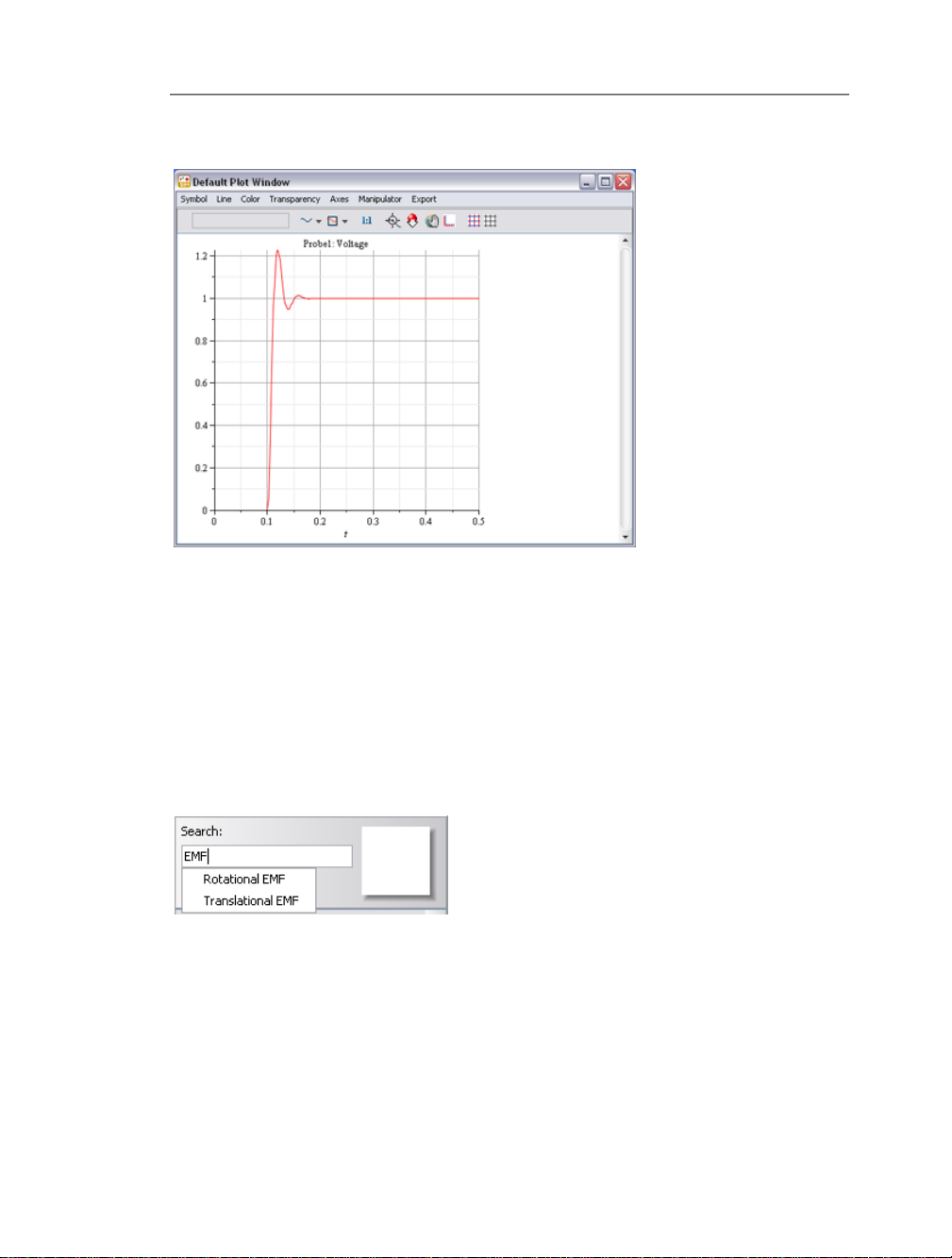
2. Inthe Inspector tab at theright of the model workspace,set the simulation end time( )
to 0.5 seconds and press Enter.
3. Click the simulation button ( ) in the main toolbar. MapleSim generates the system
equations and simulates the response to the step input.
Page 23
1.3 Basic Tutorial: Modeling an RLC Circuit and DC Motor • 13
When the simulation is complete, the voltage response is plotted in a graph.
4. Save the modelas RLC_Circuit1.msim. The probes and modied parameter values are
saved as part of the model.
Building a Simple DC Motor Model
You will now add an electromotive force (EMF) component and a mechanical inertia
component to the RLC circuit modelto create a DC motor model. Inthis example, you will
add components to the RLC circuit model using the search feature.
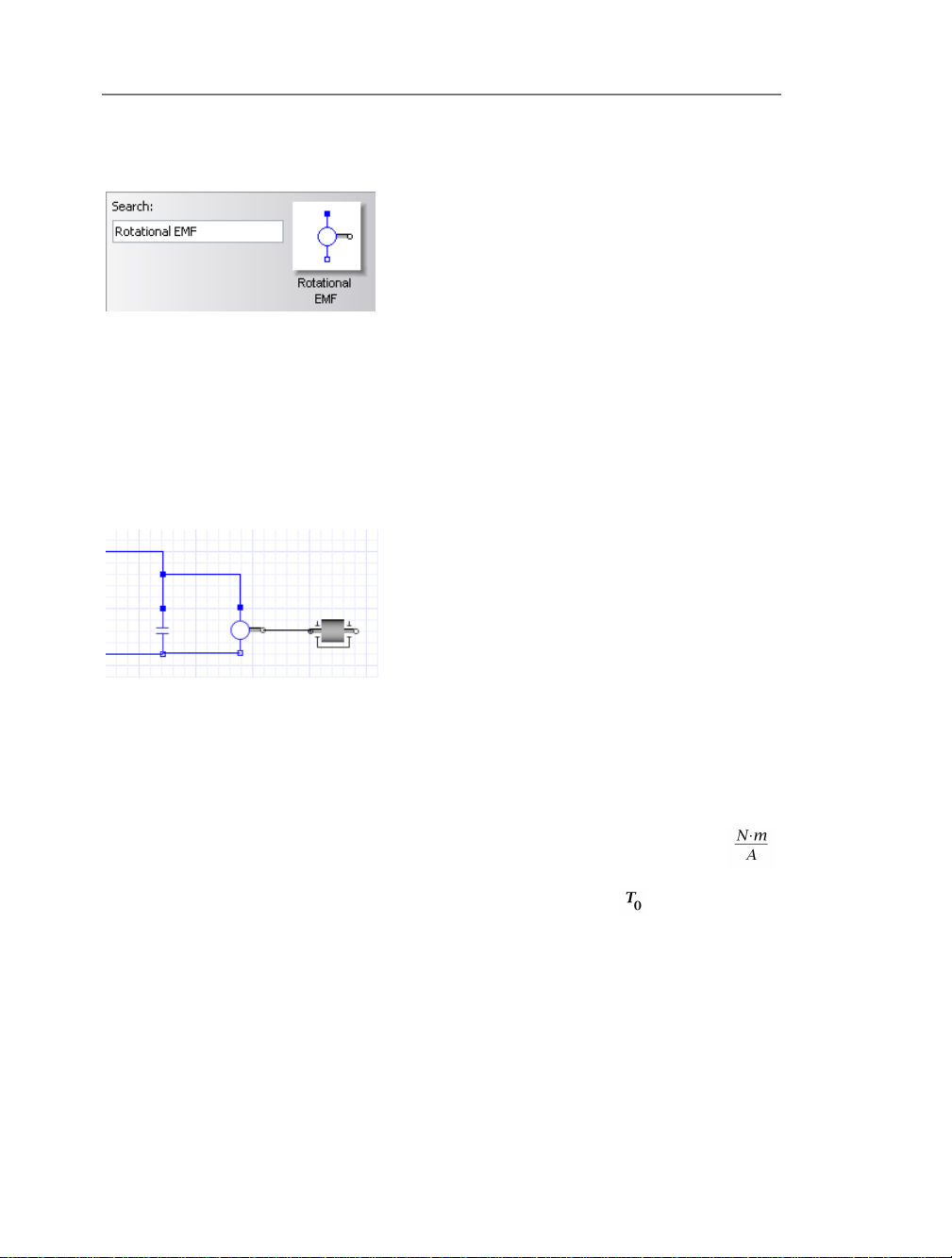
1. In the Libraries tab, in the Search eld located above the palettes, type EMF. A drop-
down list displays your search results.
Page 24
14 • 1 Getting Started with MapleSim
2. Select Rotational EMF from the drop-down list. The Rotational EMF component is
displayed in the square beside the search eld.
3. From the square beside the search eld, drag the Rotational EMF component to the
modeling workspace and place it to the right of the Capacitor component.
4. In the search pane, search for Inertia.
5. Add theInertia component to the model workspace and placeit to the right of the Rota-
tional EMF component.
6. Connect the components as shown below.
Note: To connect the positive blue port of the Rotational EMF component, click the port
once, drag your mouse pointer to the line connecting the capacitor and inductor, and click
the line.
7. In the model workspace, click the Rotational EMF component.
8. In the Inspectortab, change the value of the transformation coefcient (k) to 10 .
9. Click the Step component and change the value of the parameter, , to 1.
Page 25
1.3 Basic Tutorial: Modeling an RLC Circuit and DC Motor • 15
Simulating the DC Motor Model
1. In the model workspace, delete Probe1.
2. In the model workspace toolbar, click the probe button ( ).
3. Hover your mouse pointer over the line that connects the Rotational EMF and Inertia
components.
4. Left-click the line and then left-click the probe once to position it.
5. Select the probe.
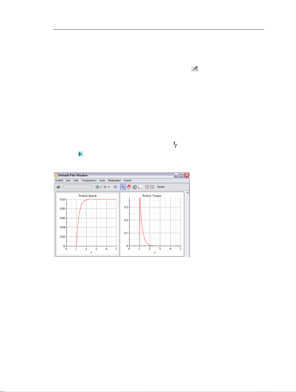
6. In the Inspectortab, selectthe Speedand Torque check boxes.The probe,with anarrow
indicating the direction of the conserved quantity ow, is added to the model.
7. Click a blank area in the model workspace.
8. In the Inspectortab, setthe simulationend time ( )to 5 seconds and clickthe simulation
button ( ) in the main toolbar.
The following graphs are displayed.
9. Save the model as DC_Motor1.msim.
Page 26

16 • 1 Getting Started with MapleSim
Page 27

2 Building a Model
In this chapter:
• The MapleSim Component Library (page 17)
• Browsing a Model (page 18)
• Dening How Components Interact in a System (page 20)
• Specifying Component Properties (page 21)
• Creating and Managing Subsystems (page 23)
• Global and Subsystem Parameters (page 34)
• Attaching Files to a Model (page 42)
• Creating and Managing Custom Libraries (page 43)
• Annotating a Model (page 45)
• Entering Text in 2-D Math Notation (page 47)
• Creating a Data Set for an Interpolation Table Component (page 48)
• Best Practices: Building a Model (page 49)
2.1 The MapleSim Component Library
The MapleSim component library contains over 300 components that you can use to build
models. All of thesecomponents are organized in palettes according to their respective domains: electrical, hydraulic, 1-D and multibody mechanical, thermal, and signal blocks.
Most of these components are based on the Modelica® Standard Library.
DescriptionLibrary
Electrical
Hydraulic
1-D Mechanical
Multibody Mechanical
Signal Blocks
Components to modelelectrical analog circuits,singlephase and multiphase systems, and electric machines.
Components to model hydraulic systems such as uid
power systems, cylinders, and actuators.
Components to model 1-D translational and rotational
systems.
Components to model multibody mechanical systems,
including force, motion, and joint components.
Components tomanipulateor generateinput andoutput
signals.
Components to model heat ow and heat transfer.Thermal
The library also contains sample models that you can view and simulate, for example,
complete electrical circuits and lters. For more information about the MapleSim library
17
Page 28

18 • 2 Building a Model
structure and modeling components, see the MapleSim Library Reference Guide in the
MapleSim help system.
To extendthe defaultlibrary,you cancreate acustom modelingcomponent froma mathematical model and add it to a custom library. For more information, see Creating Custom
Modeling Components (page 55).
Viewing Help Topics for Components
In thehelp panebelow themodel workspace,you canview thehelp topic for each component
from the MapleSimcomponent library. To display the help pane, click the help pane button
( ) at the bottom of the MapleSim window. You can then select a component that you
have addedto the modelworkspace toview itshelp topic.Alternatively, toview help topics,
you can perform one of the following tasks:
• Right-click (Control-clickfor Macintosh®)a modelingcomponent in any of thepalettes
and select Help from the context menu.
• Search for the help pages for components in the MapleSim help system.
2.2 Browsing a Model
Using the Model Tree palette or model navigation controls, you can browse your model to
view hierarchical levels of components in the modelworkspace. You can browse to the top
level for an overall view of your system. The top level is the highest level of your model:
it represents the complete system, which can include individual modeling components and
subsystem blocks that represent groups of components. You can also browse to sublevels
in your model to view the contents of individual subsystems or components.
Model Tree
To browse your model, you can use the Model Tree palette in the Project tab located on
the left side of the MapleSim window. Each node in the model tree represents a modeling
Page 29
2.2 Browsing a Model • 19
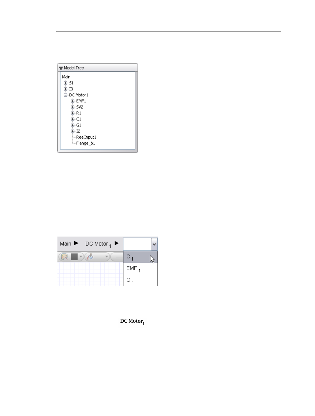
component, subsystem, or connection port in your model. For example, the model tree of
a DC motor is shown below.
To browse your model and view the parameters associated with a component or subsystem,
expand and double-click the nodes in the model tree. You can double-click the Main node
to viewthe top levelof your model and thechild nodes to view thecontents of a component
or subsystem.
Model Navigation Controls
Alternatively, youcan usethe model navigation controls located above the model workspace
toolbar to browse between modeling components, subsystems, and hierarchical levels in a
diagram displayed in the model workspace.
From the drop-down menu, select the name of the subsystem or modeling component that
you want to view in the model workspace. You can click the Main button to browse to the
top level of your model. You can also browse directly to subsystems in your model. For
example, by clicking the button in the example shown above, you can view the
DC motor subsystem contents in the model workspace.
Page 30
20 • 2 Building a Model
2.3 Defining How Components Interact in a System
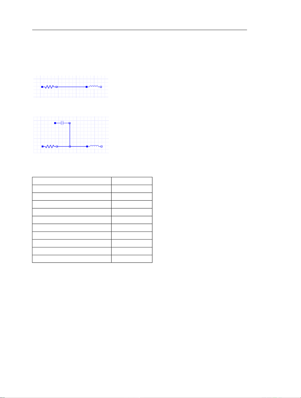
To dene interactions between modelingcomponents, you connectthem in a system. In the
model workspace, you can draw a connection line between two connection ports.
You can also draw a connection line between a port and another connection line.
MapleSim permits connections between compatible domains only. By default, each line
type is displayed in a domain-specic color.
Line ColorDomain
BlackMechanical 1-D rotational
GreenMechanical 1-D translational
BlackMechanical multibody
BlueElectrical analog
BlueElectrical multiphase
PurpleDigital logic
PinkBoolean signal
Navy blueCausal signal
OrangeInteger signal
RedThermal
The connection ports for each domain are also displayed in specic colors and shapes. For
more information about connection ports, see the MapleSim Library Reference → Con-
nectors Overview topic in the MapleSim help system.
Page 31
2.4 Specifying Component Properties • 21
2.4 Specifying Component Properties
To specify component properties, you can set parameter values for components in your
model. When you select a component in the model workspace, the congurable parameter
values for that component are displayed in the Inspector tab located on the right side of
the MapleSim window.
Note: Not all components provide editable parameter values.
You enter parameter values in 2-D math notation, which is a formatting option that allows
you to add mathematical text such as superscripts, subscripts, and Greek characters. For
more information, see Entering Text in 2-D Math Notation (page 47).
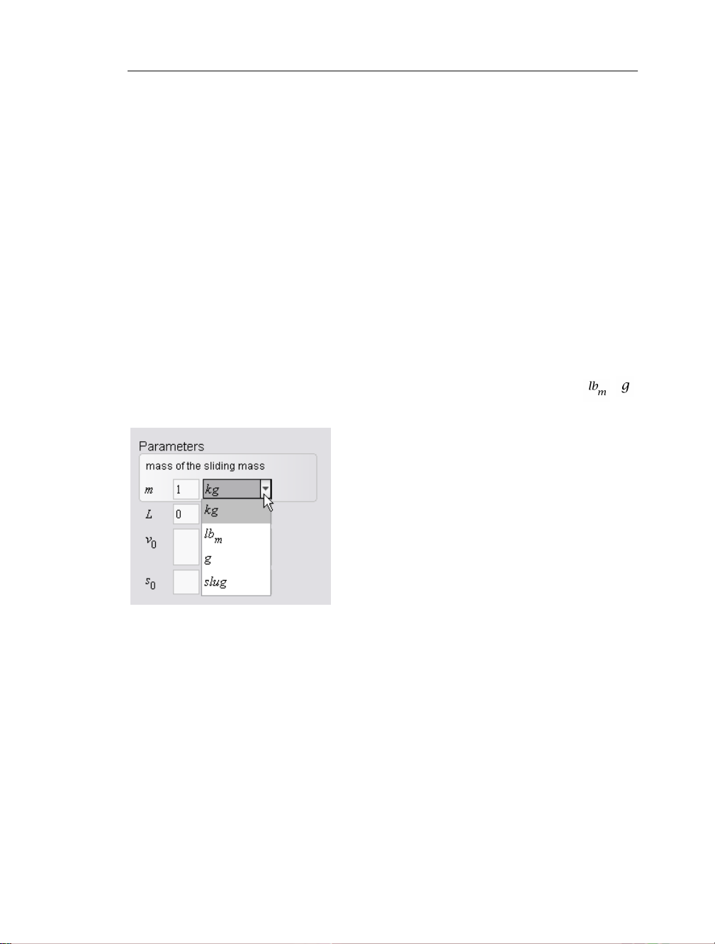
Specifying Parameter Units
You can use thedrop-down menus besideparameter elds withdimensions to specify units
for parameter values. For example, the image below displays the congurable parameter
elds for a Sliding Mass component. You can optionally specify the mass in kg, , ,
or slug, and the length in m, cm, mm, ft, or in.
When you simulate a model, MapleSim automatically converts all parameter units to the
International System of Units (SI). Youcan, therefore, selectmore than one system of units
for parameter values throughout a model.
If you want to convert the units of a signal, use the Unit Conversion Block component
from the Signal Converters menu in the Signal Blocks palette. This component allows
you to perform conversions in dimensions such as time, temperature, velocity, pressure,
and volume. In the following example, a Unit Conversion Block component is connected
Page 32

22 • 2 Building a Model
between a translational Position Sensor and Feedback component to convert the units of
an output signal.
If you include an electrical, 1-D mechanical, hydraulic, or thermal sensor in your model,
you can also select the units in which to generate an output signal.
Specifying Initial Conditions
You can set parameter values to specify initial conditions for many electrical, hydraulic,
and 1-D mechanical components, including capacitors, hydraulic pipes, and mechanical
springs and dampers. When you select a component that contains state variables in the
model workspace, the available initial condition elds are displayed in the Inspector tab,
along with the other congurable parameter values for that component.
For example, the image below displays the initial velocity and position elds that you can
set for a Sliding Mass component.
Page 33

2.5 Creating and Managing Subsystems • 23
2.5 Creating and Managing Subsystems
A subsystem (or compound component) is a set of modeling components that are grouped
in a single block component. A sample DC motor subsystem is shown below.
You can createa subsystemto groupcomponents thatform acomplete system,for example,
a tire or DC motor. You can also create a subsystem to improve the layout of a diagram in
the model workspace, add multiple copies of a system to a model, or analyze a component
group in Maple. You can organize your model hierarchicallyby creating subsystemswithin
other subsystems.
For bestpractices on creating subsystems in MapleSim, seeBest Practices: Laying Out and
Creating Subsystems (page 49).
Example: Creating a Subsystem
In the following example, you will group the electrical components of a DC motor model
into a subsystem.
1. In the Libraries tab on the left side of the MapleSim window, expand the Examples
palette, expand the Tutorial menu, and then open the Simple DC Motor example.
Page 34

24 • 2 Building a Model
2. Using the selection tool( ) located above the modelworkspace, draw abox around the
electrical components.
3. From the Edit menu, select Create Subsystem.
4. In the dialog box, enter DC Motor.
5. Click OK. A white block, which represents the DC motor, is displayed in the model
workspace.
In thisexample, you created a stand-alonesubsystem, which can be editedand manipulated
independently of other subsystems in your model. If you wantto add multiple copies of the
same subsystem to your model and edit those subsystems as a group, you can create a sub-
system denition. For more information, see Adding Multiple Copies of a Subsystem to a
Model (page 26).
Page 35

2.5 Creating and Managing Subsystems • 25
Viewing the Contents of a Subsystem
To view the contents of a subsystem, double-click the subsystem icon in the model workspace. The detailed view of a subsystem is displayed.
In this view, a broken line indicates the subsystem boundary. You can edit the connection
lines and components within the boundary, add and connect components outside of the
boundary, and add subsystem ports to connect the subsystem to other components. If you
want toresize theboundary,click thebroken line and drag oneof thesizing handlesdisplayed
around the box.
To browse to the top level of the model or to other subsystems, use the controls in the navigation toolbar.
Page 36

26 • 2 Building a Model
Adding Multiple Copies of a Subsystem to a Model
If you plan to add multiple copies of a subsystem to a model and want all of the copies to
have the same conguration, you cancreate a subsystemdenition. A subsystem denition
is the base subsystem that denes the attributes and conguration that you want a series of
subsystems to share.
For example,if you want to add three DCmotor subsystemsthat all have identical components and resistance values in your model, you would perform the following tasks:
1. Build a DC motor subsystem with the desired conguration in the model workspace
2. Use that subsystem conguration to create a subsystem denition and and add it to the
Denitions palette, and
3. Add copies of the DC motor subsystem to your model using the subsystem denition as
a source.
To add copies of the DC motor subsystem to your model, you can drag the DC Motor sub-
system denition icon from the Denitions palette and place it in the model workspace.
The copies that you add to the model workspace will then share a conguration that is
identical to the subsystem denition in the Denitions palette; the copies in the model
workspace are called shared subsystems because they share and refer to the conguration
specied in their corresponding subsystem denition.
Shared subsystems that are copied from the same subsystem denition are linked, which
means that changes that you make to one shared subsystem will be reected in all of the
other shared subsystemsthat werecreated from thesame subsystemdenition. The changes
are also reected in the subsystem denition entry in the Denitions palette.
Using the example shown above, if you change the resistance parameter of the Resistor
component in the shared subsystem from 24 to 10 , the resistance value
Page 37

2.5 Creating and Managing Subsystems • 27
of the Resistor component in the and shared subsystems and the
DC Motor subsystem denition in the Denitions palette will also be changed to 10 .
For moreinformation, see EditingSubsystem Denitions and SharedSubsystems (page 28).
Example: Adding Subsystem Definitions and Shared Subsystems to a Model
In thefollowing example,you willcreate aDC Motor subsystem denition and add multiple
shared subsystems to your model.
Adding a Subsystem Definition to the Definitions Palette
1. In the model workspace, right-click (Control-click for Macintosh) the stand-alone DC
motor subsystem that you created in Example: Creating a Subsystem (page 23).
2. From the context menu, select Convert to Shared Subsystem.
3. Enter DC Motor as the name for the subsystem denition and click OK.
4. Inthe Projecttab on the left sideof themodel workspace, expand the Denitionspalette
and then expand the Subsystems menu.
The subsystem denition is added to the Denitions palette and the subsystem in the
model workspace is converted into a shared subsystem called . This shared
subsystem is linked to the DC Motor subsystem denition.
You can now use this subsystem denition to add multiple DC motor shared subsystems
to your MapleSim model.
Page 38

28 • 2 Building a Model
Tip: If you wantto usea subsystemdenition inanother model,add thesubsystem denition
to a custom library. For more information, see Creating and Managing Custom Librar-
ies (page 43).
Adding Multiple DC Motor Shared Subsystems to a Model
To add multiple DC Motor shared subsystems to a model, drag the DC Motor subsystem
denition icon from the Denitions palette and place it in the model workspace.
When you create a new stand-alone subsystem or add shared subsystems to a model, a
unique subscript number is appended to the subsystem name displayed in the model workspace. As shown in the image above, subscript numbers are appended to the namesof each
DC Motor shared subsystem. These numbers can help you to identify multiple subsystem
copies in your model.
Editing Subsystem Definitions and Shared Subsystems
If you edit a shared subsystem in the model workspace, your changes will be reected in
the subsystem denition that is linked to the shared subsystem, as well as other shared
subsystems that were copied from the same subsystem denition.
Example: Editing Shared Subsystems that are Linked to the Same Subsystem Definition
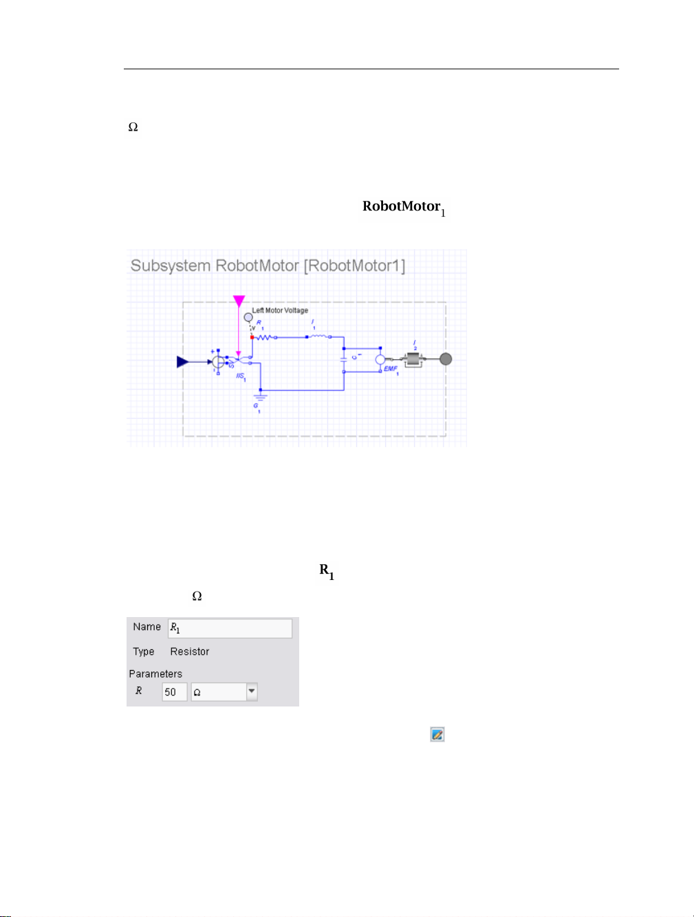
In this example, you will edit the resistance values and subsystem icons in a model that
contains two DC motor shared subsystems called and .
These shared subsystems are linked to a subsystem denition called RobotMotor. When
you changethe resistancevalue inone RobotMotorshared subsystem,the otherRobotMot-
or shared subsystem and RobotMotor shared subsystems that you add in the future will
contain the changes.
Page 39
2.5 Creating and Managing Subsystems • 29
To start, both RobotMotor shared subsystems in this model have a resistance value of 30
.
1. In the Libraries tab on the left side of the MapleSim window, expand the Examples
palette, expand the Multidomain menu, and then open the Sumobot example.
2. Inthe model workspace,double-click the shared subsystem.The detailed
view of the shared subsystem is displayed.
Note that a heading with the subsystem denition name (RobotMotor) followed by the
shared subsystem name (RobotMotor1) is displayed at the top of the model workspace.In
the detailed view of all shared subsystems, this heading is displayed to help you identify
multiple subsystem copies in your model. Also, when you select a shared subsystem, its
subsystem denition name is displayed in the Type eld in the Inspector tab.
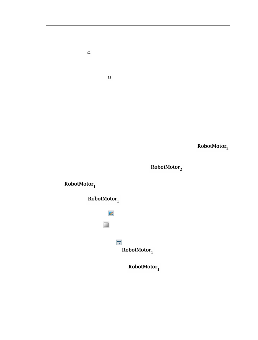
3. Select the Resistor component ( ) and, in the Inspector tab, change the resistance
value to 50 .
4. In the navigation toolbar, click the icon view button ( ).
Page 40

30 • 2 Building a Model
5. Using the rectangle tool( ) in themodel workspace toolbar, click and dragyour mouse
pointer to draw a shape in the box.
6. In the navigation toolbar, click the diagram view button ( ).
7. Click Main in the navigation toolbar to browse to the top level of the model. Both of the
RobotMotor shared subsystems now display the square that you drew.
8. In the Project tab on the left side of the MapleSim window, expand the Denitions
palette, and thenexpand theSubsystems menu. As shown inthe imagebelow,your changes
are also reected in the RobotMotor entry displayed in this palette.
Page 41
2.5 Creating and Managing Subsystems • 31
If you double-click the RobotMotor subsystems in the model workspace and select their
Resistor components, you will also see that both of the shared subsystems now have a res-
istance value of 50
9. From the Denitions palette, drag a new copy of the RobotMotor subsystem and place
it anywhere in the model workspace. The new copy displays the square that you drew and
its resistance value is also 50
Example: Removing the Link Between a Shared Subsystem and its Subsystem Definition
If your model contains multiple shared subsystems that are linked and youwant to edit one
copy only, you canremove thelink betweena sharedsubsystem andits subsystem denition,
and edit that subsystem without affecting others in the model workspace.
1. In the Libraries tab on the left side of the MapleSim window, expand the Examples
palette, expand the Multidomain menu, and then open the Sumobot example.
2. In the model workspace, right-click (Control-click for Macintosh) the
shared subsystem.
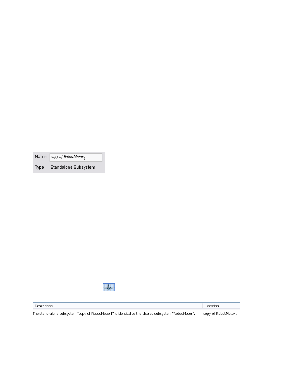
3. Select Convertto Stand-alone Subsystem. The subsystem isno longer
linked to the RobotMotor subsystem denition in the Denitions palette; it is now called
copy of
4. Double-click the shared subsystem.
5. Click the icon view button ( ).
6. Using the rectangle tool ( ), click and drag your mouse pointer to draw a shape in the
box in the model workspace.
7. Click the diagram view button ( ) and click Main to browse to the top level of the
model. Your change is shown in the shared subsystem in the model
workspace and the RobotMotor subsystem denition in the Denitions palette. Note that
your changeis notshown inthe copyof subsystem thatis nolonger linked
to the RobotMotor subsystem denition.
Page 42
32 • 2 Building a Model
Tip: When you converta shared subsystem to astand-alone subsystem,it is a good practice
to assign the stand-alone subsystem a meaningful name that clearly distinguishes it from
existing shared subsystems and subsystem denitions.
Working with Stand-alone Subsystems
Stand-alone subsystems are subsystems that are not linked to a subsystem denition. You
can create a stand-alone subsystem in two ways: by creating a new subsystem as shown in
Example: Creating a Subsystem (page 23) or by converting a shared subsystem to a standalone subsystem as shown in Example: Removing the Link Between a Shared Subsystem
and its Subsystem Denition (page 31). Stand-alone subsystems can be edited independently
without affecting other subsystems in the model workspace.
To identify a subsystem as a stand-alone subsystem, select a subsystem in the model
workspace and examine the Inspector tab. If that subsystem is a stand-alone subsystem,
the Type eld reads Standalone Subsystem.
Also, ifyou double-clicka stand-alonesubsystem tobrowse toits detailedview,no heading
is displayed for the subsystem in the model workspace.
When youcopy andpaste astand-alone subsystem in the model workspace, you can optionally convert that subsystem into a shared subsystem and createa new subsystem denition.
For more information, see Example: Copying and Pasting a Stand-alone Subsys-
tem (page 33).
Example: Resolving Warning Messages in the Debugging Console
When you convert a shared subsystem into a stand-alone subsystem, a warning message
appears to inform you that the link to the subsystem denition has been removed.
Note: This example is an extension of Example: Removing the Link Between a Shared
Subsystem and its Subsystem Denition (page 31).
1. Click the debugging button ( ) at the bottom of the MapleSim window todisplay the
debugging console. The following warning message appears in the console.
Page 43
2.5 Creating and Managing Subsystems • 33
2. To work with the copy of subsystem as a stand-alone subsystem, rightclick (Control-click for Macintosh) the warning message and select Ignore duplication
warnings for “copy for RobotMotor1”.
Alternatively, if you want to link the copy of stand-alone subsystem to the
RobotMotor subsystem denition again,you canright-click (Control-clickfor Macintosh)
the warning message and select Update “copy of RobotMotor1” to use the shared sub-
system “RobotMotor”.
Example: Copying and Pasting a Stand-alone Subsystem
Note: This example is an extension of Example: Removing the Link Between a Shared
Subsystem and its Subsystem Denition (page 31).
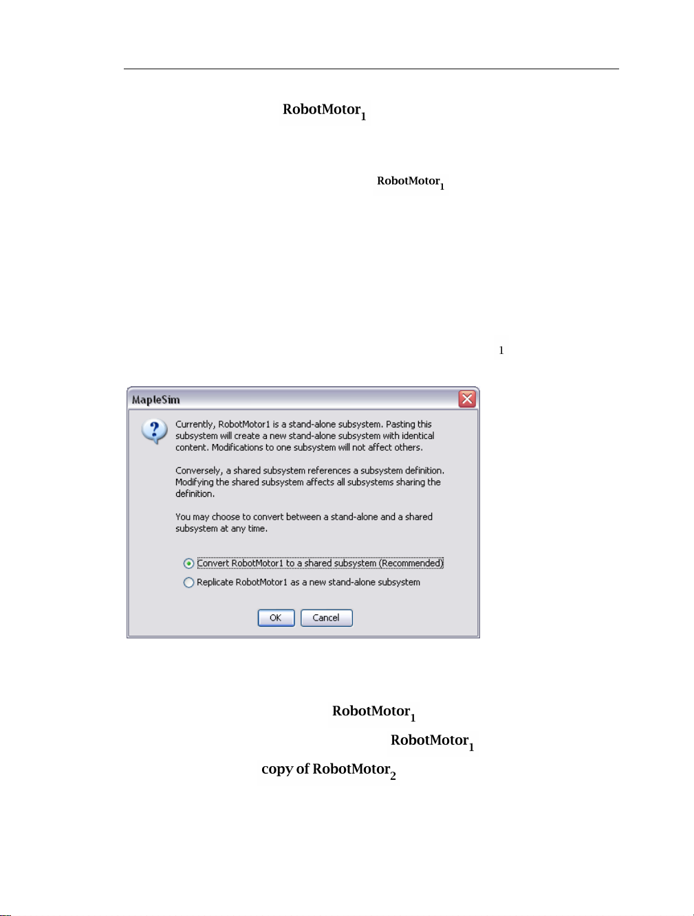
1. Inthe model workspace,copy and paste the copyof RobotMotor stand-alone subsystem. The following dialog box is displayed:
2. SelectConvert RobotMotor 1 to shared subsystem (Recommended). Anew subsystem
denition called RobotMotor 1 is added to the Denitions palette.
In the model workspace, the copy of stand-alone subsystem has been
converted to a shared subsystem called copy of and another copy of that
shared subsystemcalled has beenadded to themodel workspace.
Page 44

34 • 2 Building a Model
Both the copy of and shared subsystems are
linked to the new RobotMotor 1 subsystem denition. Therefore, if you edit either
or in the model workspace, your
changes will not be reected in subsystems that are linked to the original RobotMotor
subsystem denition.
Note: Alternatively, you can select Replicate RobotMotor 1 as a new stand-alone subsystem to add another stand-alone subsystem that can be edited independently without af-
fecting other subsystems in the model workspace.
2.6 Global and Subsystem Parameters
Global Parameters
If yourmodel contains multiplecomponents thatshare a commonparameter value, you can
create a global parameter. A global parameter allows you to dene a common parameter
value in one location and then assign that common value to multiple components in your
model.
The example described below illustrates how to dene and assign a global parameter. To
view a more detailed example, see Tutorial 1: Modeling a DC Motor with a Gear-
box (page 105) in Chapter 6 of this guide.
Example: Defining and Assigning a Global Parameter
If yourmodel containsmultiple Resistorcomponents thathave acommon resistancevalue,
you can dene a global parameter for the resistance value in the parameter editor view.
1. In the Libraries tab, expand the Electrical palette, expand the Analog menu, expand
the Passive menu, and then expand the Resistors menu.
2. Fromthe palette, drag three copiesof the Resistor component into the model workspace.
Page 45

2.6 Global and Subsystem Parameters • 35
3. In the navigation toolbar, click the parameter editor button ( ). You will use this screen
to dene the global parameter and assign it to the Resistor components in your model.
4. Click the rst eld in the Main subsystem default settings table.
5. Enter GlobalResistance as the global parameter name and press Enter.
6. Specify a default value of 2 and enter Global resistance variable as the description.
The global parameter for the resistance value is now dened. You can now assign the
common GlobalResistance parameter value to the individual Resistor components that
you added to the model workspace.
Page 46
36 • 2 Building a Model
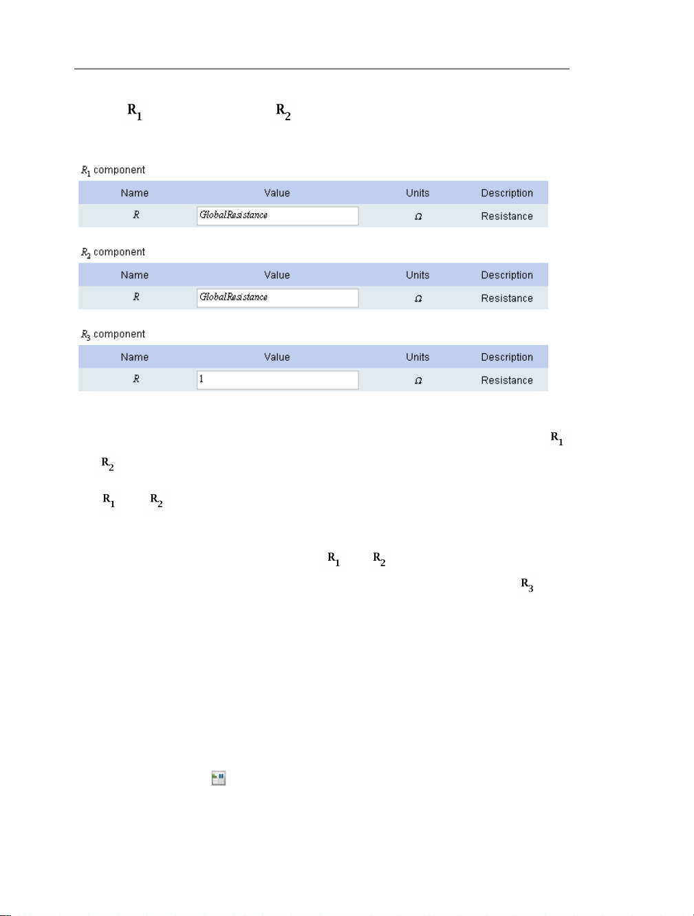
7. In the component table and component table, enter GlobalResistance as the
resistance value.
The resistancevalue of the parameter GlobalResistance (2, as dened in theMain subsys-
tem default settings table) has now been assigned to the resistance parameters of the
and components.
The and components will now inherit any changes made to the GlobalResistance
parameter value in the Main subsystem default settings table. For example, if you change
the default value of the GlobalResistance parameter to 5 in the Main subsystem default
settings table, the resistanceparameters ofthe and componentswill alsobe changed
to 5. Any change to the GlobalResistance parameter value will not apply to the component because it has not been assigned GlobalResistance as a parameter value.
Subsystem Parameters
You can create asubsystem parameter ifyou want to create a common parameter value that
will be shared by multiple components in a subsystem. Similar to global parameters, a
subsystem parameter is a common value that you dene in the parameter editor view and
assign to components.
Subsystem parameters, however, can only be assigned to components in the subsystem in
which they are dened. If you double-click a subsystem in the model workspace, click the
parameter editor button ( ), and dene a parameter in the parameter editor view, the
Page 47

2.6 Global and Subsystem Parameters • 37
parameter that you dene can only be assigned to components in the subsystem that you
double-clicked and any nested subsystems.
To view an example, see Tutorial 3: Modeling a Nonlinear Damper (page 114) in Chapter
6 of this guide.
Note: If you create a parameter within a subsystem and assign its value to a component at
the top level, the component at the top level will not inherit the parameter value.
Example: Assigning a Subsystem Parameter to a Shared Subsystem
If you assign a subsystem parameter to a shared subsystem in your model, the default subsystem parameter will also be assigned to other shared subsystems that are linked to it.
However, after the default subsystem parameter is assigned, you can edit the subsystem
parameter value for each shared subsystem separately without affecting other parameter
values in the model.
1. Inthe Examplespalette, expandthe Multibodysubmenu, andopen theDouble Pendulum
model. This model contains two shared subsystems, and , which are linked to a
subsystem denition called L.
2. Double-click the shared subsystem.
3. Click the parameter editor button ( ).
4. In the L subsystem default settings table, click the empty eld at the bottom of the
table.
5. Type c as the parameter name, keep the default value as 1, and press Enter.
6. Click thediagram view button ( ). The new subsystem parameter, c, is displayed in the
Inspector tab for the shared subsystem.
7. In the top view of the model, select the subsystem and examine the Inspector tab.
The new subsystem parameter is also displayed for the shared subsystem.
8. In the Inspector tab, change the value of c to 50.
9. Click the shared subsystem in the model workspace and examine the Inspector tab.
Note that the value of its parameter, c, remains the same.
Page 48
38 • 2 Building a Model
Creating Parameter Blocks
As analternative todening subsystemparameters usingthe methodsdescribed above,you
can create a parameter block to dene a set of subsystem parameters and assign them to
components in your model. Parameter blocks allow you to reuse sets of parameter values
in multiple models.
The followingimage shows a parameter blockthat hasbeen added tothe modelworkspace.
When youdouble-click this block, the parametereditor view is displayed. Thisview allows
you to dene parameter values for the block.
After dening parameter values, you can assign those values to the component parameters
in your model.
To useparameter valuesin another model, you can add aparameter blockto acustom library.
For more information about custom libraries, see Creating and Managing Custom Librar-
ies (page 43).
Notes:
• Parameter blocks must be placed in thesame subsystem as the components to whichyou
want to assign the parameter value.
• Parameter blocks atthe samehierarchical levelin amodel cannothave thesame parameter
names. For example, two separate parameter blocks in the same subsystem cannot each
contain a parameter called mass.
Example: Creating and Using a Parameter Block
In thisexample, youwill createa setof parameters that can be shared bymultiple components
in your model. By creating a parameter block, you only need to edit parameter values in
one location to compare results when you run multiple simulations.
Page 49

2.6 Global and Subsystem Parameters • 39
1. In the Libraries tab on the left side of the MapleSim window, expand the Examples
palette, expand the Mechanical menu, and then open the PreLoad example.
2. From the model workspace toolbar, click the parameter block button ( ).
3. Click a blank area in the model workspace. The Create Parameter Block dialog box is
displayed.
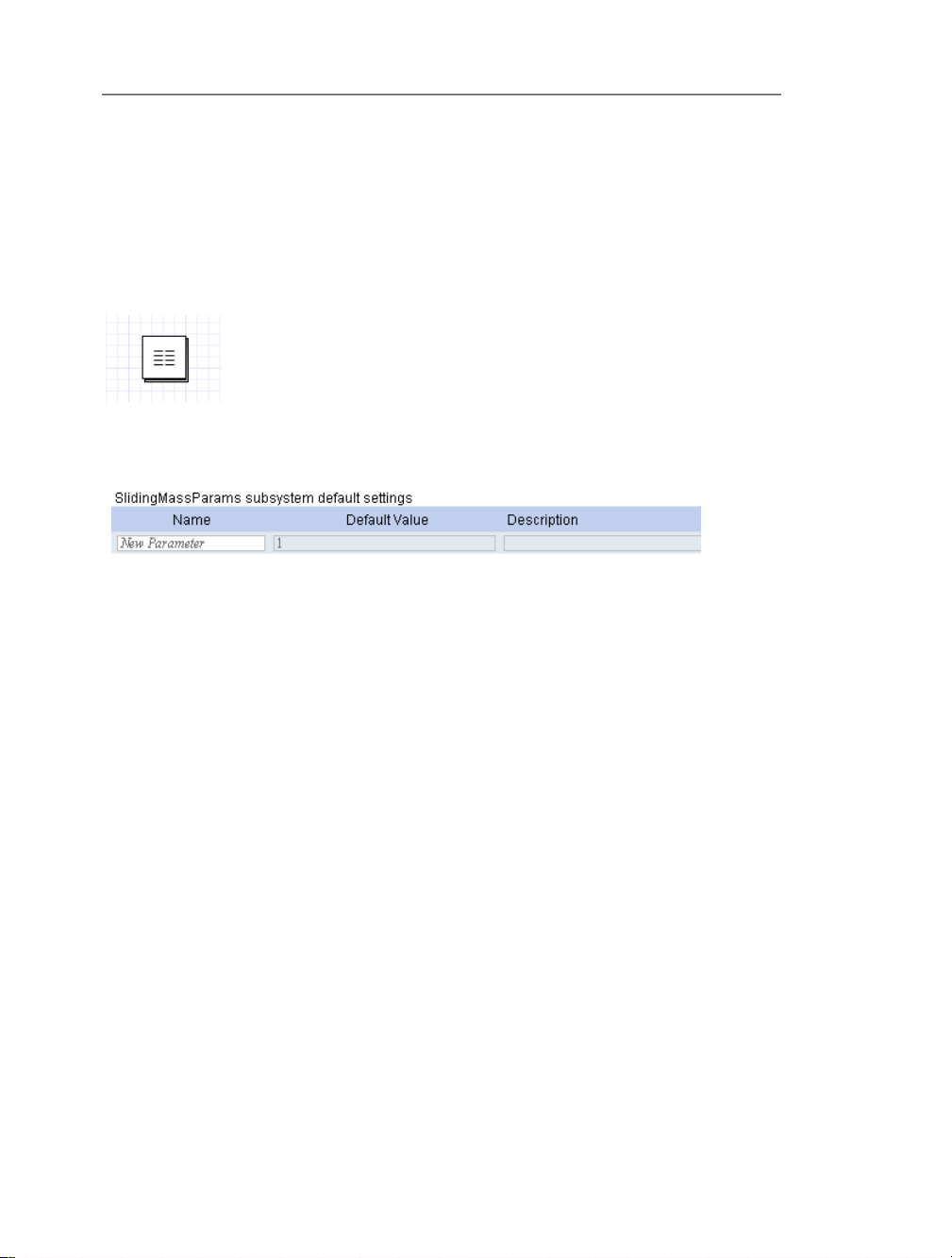
4. Specify a parameter block name SlidingMassParams and click OK.
5. Double-click the SlidingMassParams parameter block in the model workspace. The
parameter editor view is displayed.
6. Click the rst eld in the table and dene a new parameter called MASS.
7. Press Enter.
8. Specify a default value of 5 and enter the description Mass of the sliding mass.
9. In thesame way, dene the following parameters andvalues in the SlidingMassParams
subsystem default settings table.
Name
Value
DescriptionDefault
Length of the sliding mass.2LENGTH
Initial velocity of the sliding mass.1
Initial position of the sliding mass.1
Tip: To enter a subscript, press Ctrl + Shift + the underscorekey (Windows® andLinux®)
or Command + Shift + the underscore key (Macintosh®) and type the valueto include in
Page 50

40 • 2 Building a Model
the subscript. To move the cursor outof the subscript position, press the right arrow key on
your keyboard.
The parameter editor view appears as follows when the values are dened.
10. Clickthe diagram view button ( ) andthen clickMain in the navigationtoolbar.When
you select the parameter blockin the modelworkspace, the parametersthat you denedare
displayed in the Inspector tab on the right side of the MapleSim window.
11. In the model workspace, select one of the Sliding Mass components in the diagram.
12. In the Inspector tab, assign the following values.
Page 51

2.6 Global and Subsystem Parameters • 41
The parameters of this Sliding Mass component now inherit the numeric values that you
dened in the parameter block.
13. In the same way, assign the same values to the parameters of the other Sliding Mass
components in the model.
14. In the model workspace, delete Probe1.
15. Select Probe2.
16. In the Inspector tab, clear the check box beside Speed.
17. To simulate themodel, clickthe simulationbutton ( ) in themain toolbar. Thefollowing
graph is displayed.
18. In the model workspace, click the parameter block.
19. In the Inspector tab, change the mass to 25, the length to 10, and the initial velocity to
5. These changes apply to all of the Sliding Mass components to which you assigned the
symbolic parameter values.
Page 52

42 • 2 Building a Model
20. Simulate the model again. Another simulation graph, which you can compare to your
rst rst graph, is displayed. In this example, the curve shifts vertically after you run a
simulation with the new parameter values.
2.7 Attaching Files to a Model
You can use the Attachments palette in the Project tab to attach les of any format to a
model (for example, spreadsheets or design documents created in external applications).
You can save les attached in the Attachments palette as part of the current model and
refer to them when you work with that model in a future MapleSim session. To save a le,
right-click (Control-click forMacintosh) thecategory in whichyou wantto savethe attachment in the palette and select Attach File.
The following is an image of an Attachments palette that contains les called Damper-
Curve.csv and Data Generation.mw.
You can alsouse the Attachments palette to open MapleSim templates to perform analysis
tasks in Maple, create custom modeling components, and generate data sets for a model.
Page 53

2.8 Creating and Managing Custom Libraries • 43
For more information about performing analysis tasks, see Analyzing and Manipulating a
Model (page 97) in this guide.
2.8 Creating and Managing Custom Libraries
You can create a custom library to save a collection of subsystems, custom modeling components, orattachments thatyou planto reusein multipleles or MapleSim sessions. Custom
libraries are displayed in custom palettes below the Examples palette, in theLibraries tab,
on the left side of the MapleSim window and saved as .msimlib les on your computer.
A sample custom palette with a subsystem is shown below.
Example: Adding Subsystems and Attachments to a Custom Library
In this example, you will add a subsystem and an .mw attachment to a custom library to
make them available in a future MapleSim session.
1. In the Libraries tab, expand the Examples palette, expand the Multidomain menu, and
then open the Sliding Table example.
2. From the File menu, select Create Library...
Page 54

44 • 2 Building a Model
3. Select a path and specify the le name Sliding Table.msimlib.
Note: This le will store the custom library and the le name that you specify will appear
as the custom palette name in the MapleSim interface.
4. Click Save. The Add to User Library dialog box displays all of the subsystems in your
model and les attached in the Attachments palette.
5. Select the check box beside Motor to add the subsystem to the custom library.
6. Select the check box besideAdvancedAnalysis.mw to add theattachment to the custom
library.
7. Click OK. A new custom library palette is added in the Libraries tab on the left side of
the MapleSim window.
Page 55

2.9 Annotating a Model • 45
This palette and its contents are displayed in the Libraries tab. They can be used in a
model the next time you start MapleSim.
8. In the Sliding Table palette, click Attachments. The Library Attachments dialog box
is displayed. This dialog box lists all of the attachments that you have added to the custom
library.
You can also use this dialog box to add attachments to the Attachments palette of another
model and open attachments in their associated applications.
9. Close the dialog box.
2.9 Annotating a Model
You can use the tools in the model workspace toolbar to draw lines, arrows, and shapes.
MapleSim also provides many tools for customizing the colors, line styles, and shape lls.
You can use the text tool ( ) in the model workspace toolbar to add text annotations to
your model. In text annotations, you can enter mathematical text in 2-D math notation and
Page 56

46 • 2 Building a Model
modify the style, color, and font of the text. For more information about 2-D math notation,
see Entering Text in 2-D Math Notation (page 47).
Example: Adding a Text Annotation to a Model
1. In the Libraries tab, expand the Examples palette, expand the Tutorial menu and then
open the Simple DC Motor example.
2. From the model workspace toolbar, click the text tool button ( ).
3. In the model workspace, draw a text box for an annotation below the Step component.
When you releaseyour left mouse button, the toolbar above the model workspace switches
to the text formatting toolbar.
4. Enter the following text: This block generates a step signal with a height of 1.
5. Select the text that you entered and change the font to Arial.
6. Click anywhere outside of the text box.
7. Draw another text box below the Inertia component.
8. Enter the following text: Inertia with a value of 0 rad.
Tip: To enter the omega character ( ), press F5 to switch to the 2-D math mode, type
omega, and then press Ctrl + Space (Windows), Ctrl + Shift + Space (Linux), or Esc
(Macintosh). To enter the subscript, press Ctrl + Shift + the underscore key (Windows
and Linux) or Command + Shift + the underscore key (Macintosh) followed by 0. Press
the right arrow key to move the cursor from the subscript position.
9. Click anywhere outside of the text box.
Page 57

2.10 Entering Text in 2-D Math Notation • 47
10. Select the text that you entered and change the font to Arial.
11. Click anywhere outside of the text box to complete the annotation.
2.10 Entering Text in 2-D Math Notation
In parameter values and annotations, you can enter text in 2-D math notation, which is a
formatting option for adding mathematical elements such as subscripts, superscripts, and
Greek characters. As you enter a phrase in 2-D math notation, you can use the command
and symbol completion feature to display a list of possible Maple commandsor mathematical symbols that you can insert.
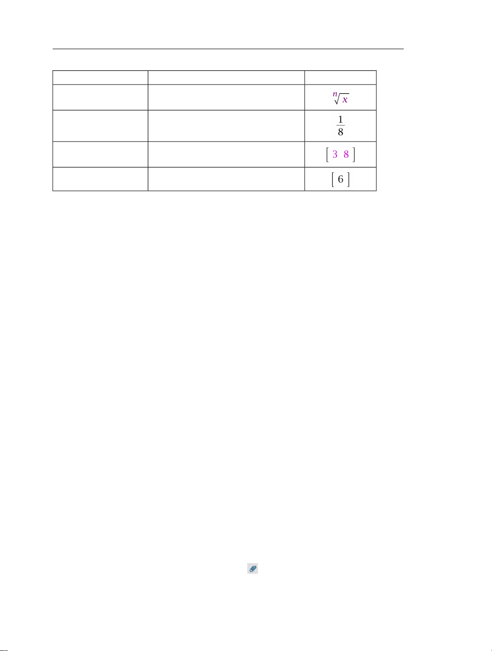
The following table lists common key combinations for 2-D math notation:
ExampleKey CombinationTask
Switch between text and
2-D math mode (annotations only)
Command and symbol
completion (parameter
values and annotations
only)
Enter a subscript for a
variable
1. Enter the rst few characters of a symbol
name, Greek character, or Maple command.
2. Enter the key combination for your platform:
• Ctrl + Space (Windows)
• Ctrl + Shift + Space (Linux)
• Esc (Macintosh)
3. From the menu, select the symbol or
command that you want to insert.
Ctrl (or Command) + Shift + underscore
( _ )
-F5
-
Enter a square root
caret (^)Enter a superscript
Enter sqrtand pressCtrl (or Command for
Macintosh) + Space.
Page 58
48 • 2 Building a Model
Enter a root
Enter nthroot and press Ctrl(or Command)
+ Space.
forward slash (/)Enter a fraction
ExampleKey CombinationTask
Enter a piecewise, matrix,
or vector row
For more information, see the Using MapleSim → Building a Model → Annotating a
Model → Key Combinations for 2-D Math Notation topic in theMapleSim help system.
Ctrl (or Command) + Shift + R
Ctrl (or Command) + Shift + CEnter a table column
2.11 Creating a Data Set for an Interpolation Table
Component
You can create a data set to provide values for an interpolation table component in your
model. Forexample, youcan providecustom values for input signals, and electricalCurrent
Table and Voltage Table sources. To create a data set, you can either attach a Microsoft®
Excel® spreadsheet (.xls) or comma-separated values (.csv) le that contains the custom
values, or youcan createa dataset in Mapleusing theData Generation Template or Random
Data Template provided in the MapleSim templates dialog box.
Note: The Microsoft Excel 2007 le format (.xlsx) is not supported.
For more information about interpolation table components, see the MapleSim Library
Reference →Signal Blocks → Interpolation Tables→ Overview topic in the MapleSim
help system.
Example: Creating a Data Set in Maple
In this example, you will use the Data Generation Template to create a data set for a
MapleSim 1DLookup Tablecomponent. Inthis template,you canuse anyMaple commands
to create a data set; however, for demonstration purposes, you will create a data set using
a computation that has already been dened.
1. Open a new MapleSim document.
2. Inthe Librariestab, expandthe Signal Blocks palette, andthen expandthe Interpolation
Tables menu.
3. Add a 1D Lookup Table component to the model workspace.
4. In the main toolbar, click the templates button ( ).
Page 59

2.12 Best Practices: Building a Model • 49
5. From the templates list, select Data Generation.
6. In the Attachment eld, enter My First Data Set and click Create Attachment. The
Data Generation Template is opened in Maple.
7. To execute the entire worksheet, click at the top of the Maple window.
8. At the bottom of the template, in the Data set name eld, enter TestDataSet.
9. To make the data set availablein MapleSim, clickthe Attach Data in MapleSim button.
10. In MapleSim, in the Project tab, expand the Attachmentspalette, and then expand the
Data Sets category. The data set le is displayed in the list.
You can nowassign thisdata set to the interpolation table component in themodel workspace.
11. In the model workspace, select the 1D Lookup Table component.
12. Inthe Inspectortab, from the data drop-down menu, selectthe TestDataSet.mpld le.
The data set is now assigned to the 1D Lookup Table component.
13. Save the Data Generation Template in Maple and then save your model in MapleSim.
2.12 Best Practices: Building a Model
This section describes best practices to consider when laying out and building a MapleSim
model.
Best Practices: Laying Out and Creating Subsystems
To start building your model, drag components from the palettes to the center of the model
workspace. Dragthe componentsinto thearrangement thatyou wantin themodel workspace
and then, if necessary, change their orientation so that the components are facing in the
direction that you want. When you have established the position and orientation of the
components, connect them in the model workspace.
When groupingcomponents intosubsystems, makesure thatyou includelogical component
groupings that t on one screen at a time. This will allow you to see all of the subsystem
components at a certain level without scrolling.
Create Subsystems for Component Groups That You Plan to Reuse
Create subsystems for component groups that you plan to reuse throughout a diagram or in
multiple les.For example,if youplan to include multiple planarlink modelsin apendulum
system, you can create a link subsystem so that multiple copies of that component group
could be added. If you wanted to add the link subsystem to another pendulum model, you
can create a custom library to use the subsystem in another le.
Page 60
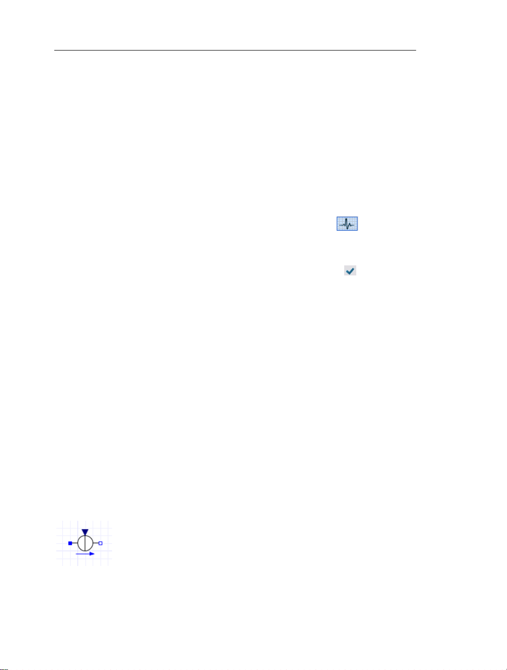
50 • 2 Building a Model
Create Subsystems for Component Groups That You Plan to Analyze
Make sure that you create subsystems for component groups that you plan to analyze in
more depth, test, or translate into source code. Several MapleSim templates allow you to
analyze and retrieve equations from particular subsystems. The Code Generation Template
allows you to generate source code from subsystems only.
For more information about performing analysis tasks, see Analyzing and Manipulating a
Model (page 97) in this guide.
Use the Debugging Console to Identify Subsystem Copies and Unconnected
Lines
You can display the debugging pane by clickingthe debugging button( ) atthe bottom
of the MapleSim window.
The debugging pane displays diagnostic messages that can help you troubleshoot potential
errors as you build a model. When you click the diagnostic tests button ( ) below the debugging pane,MapleSim verieswhether yourmodel containsunconnected linesor subsystems that have identical content but are not linked to a subsystem denition. When either
of these issues are detected, a message that identies the subsystem in which the issue is
located is displayed in the debugging console. You can right-click (Control-click for
Macintosh) themessage inthe debuggingpane todisplay options that can helpyou toresolve
the issue.
Best Practices: Building Electrical Models
Include a Ground Component in Electrical Circuits
In eachelectrical circuit model, you mustadd and connect a Ground component toprovide
a reference for the voltage signals.
Verify the Connections of Current and Voltage Sources
Simulation results can be affected by the way in which a current or voltage source is connected in your model. If you receive unexpected simulation results, verify the connections
between electrical sources and other components in your model. All of the current sources
in the MapleSim component library display an arrow that indicates the direction of the
positive current.
Page 61
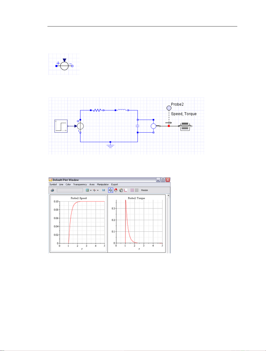
2.12 Best Practices: Building a Model • 51
Also, all of the voltage sources display a plus sign indicating the location of the positive
voltage and a minus sign indicating the location of the negative voltage.
Consider the following DC motor model. Note that the positive port of the Signal Voltage
source atthe leftof thediagram is connected to the positive port of the Resistor component.
When this model is simulated, MapleSim returns the following results for the speed and
torque quantities.
Page 62

52 • 2 Building a Model
On the other hand, if the negative port of the Signal Voltage source is connected to the
positive port of the Resistor component, as shown in the following image
MapleSim returns different results for the speed and torque quantities.
Best Practices: Building 1-D Translational Models
Verify That All Force Arrows Are Pointed in the Same Direction
In MapleSim, all of the 1-D translational mechanical components are dened in a 1-D coordinate system with the positive direction dened as the direction of the gray arrow displayed by the component icon.
Any positive forces acting on the model cause the component to move in the direction of
the arrow, so make surethat all ofthe arrows displayedby the 1-Dtranslational mechanical
Page 63
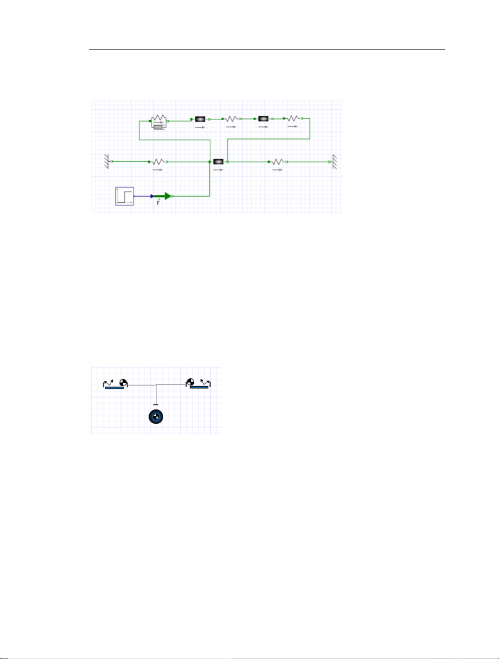
2.12 Best Practices: Building a Model • 53
components in your model point in the same direction. As an example, note that all of the
force arrows are pointed to the right in the following multiple mass spring-damper model.
Best Practices: Building Multibody Models
Connect the Inboard Port of a Rigid Body Frame to a Center-of-mass Frame
Make surethat youconnect the inboard port of any RigidBody Frame components in your
model to the center-of-mass frame of a Rigid Body component. This ensures that the local
reference frame used to describe displacements and rotations for the Rigid Body Frame
component match with the center-of-mass reference frame dened on the Rigid Body
component.
In thefollowing planarlink example, the Rigid Body Frame inboard ports(that is,the ports
with the cross-hatched circles) are both connected to a Rigid Body component.
Best Practices: Building Hydraulic Models
Define Fluid Properties
When building hydraulic models, you must dene the properties of the uid that will be
used by placing the Hydraulic Fluid Properties component at the top level of your model
or at same level as a hydraulic subsystem. If you place this component at the top level of
your model, all hydraulic components and subsystems in your model will inherit the uid
properties denedby thatcomponent instance;if you place the Hydraulic Fluid Properties
component at the same level as a subsystem, all hydraulic components in that subsystem
and all nested subsystems will inherit the properties dened by that component instance.
Page 64

54 • 2 Building a Model
In the following example, all of the hydraulic components in the model inherit the uid
properties dened by the Hydraulic Fluid Properties component at the top-right of the
diagram.
Page 65

3 Creating Custom Modeling Components
In this chapter:
• Overview (page 55)
• Opening Custom Component Examples (page 56)
• Example: Nonlinear Spring-Damper Component (page 56)
• Working with Custom Components in MapleSim (page 61)
• Editing a Custom Component (page 62)
3.1 Overview
To extend the MapleSim component library, you can create custom modeling components
based on mathematical models that you dene. For example, you can create a custom
component to contain a particular subsystem and to provide specialized functionality.
By using the Custom Component Template, which is a Maple worksheet available through
the MapleSim templates dialog box, you perform the following tasks in Maple to create a
custom component:
• Dene the component equations and properties that determine the behavior of the component (for example, parameters and port variables)
• Test and analyze your mathematical model
• Add ports to the component and dene the associated port variable mappings
• Generate the component and make it available in MapleSim
The Custom Component Template contains pre-built controls that allow you to perform
these tasks. Each generated custom component is associated with a particular template.
55
Page 66

56 • 3 Creating Custom Modeling Components
3.2 Opening Custom Component Examples
The following custom component examples are available with yourMapleSim installation:
• Custom component dened with an algebraic equation
• A sample DC motor component dened with a differential equation
• A sample nonlinear spring-damper component
• Custom component dened with a transfer function
To open an example:
1. In MapleSim, click the templates button ( ) in the main toolbar.
2. Click Browse...
3. In the Browse Templates dialog box, open the Component Templates folder.
4. Select the example that you want to open, and click Use Template
5. In the Attachment eld, enter a name for the template.
6. ClickCreate Attachment. The sample Custom Component Template isopened inMaple.
3.3 Example: Nonlinear Spring-Damper Component
In thisexample, youwill use the Custom ComponentTemplateto createa nonlinearspringdamper custom component. The equations dened in this example are based on the
Translational Spring Damper component in MapleSim. In this case, the stiffness and
damping coefcients are replaced with input functions to the component.
Page 67

3.3 Example: Nonlinear Spring-Damper Component • 57
To obtain thegoverning relationships, youcan start witha free-body diagram.The diagram
for the spring-damper system is shown below.
The end points, a and b, can be dened as the ports for the component; the equations are
derived relative to these ports. Therefore, the general equation of motion,
where is the damping coefcient, is thestiffness ofthe spring,and is therelative
displacement between the two ports and , can be written as
Also, an examination of the net force on the system shows that , where
All of the above relationships are required to dene the system behavior.
Page 68

58 • 3 Creating Custom Modeling Components
Opening the Custom Component Template
To start, open the Custom Component Template from the MapleSim templates dialog box.
1. In MapleSim, open the model to which you want to add the custom component.
2. Click the templates button ( ) in the main toolbar.
3. In the Standard Templates list, select Custom Component.
4. In the Attachment eld, enter Nonlinear Spring-Damper as the name for the template
and click Create Attachment. The Custom Component Template is opened in Maple.
Defining the Component Name and Equations
You can now specify the name that will be displayed for the component in the MapleSim
interface, a variable to store the equations, and the equations.
To dene the component equations, you create a system model by using commands from
the DynamicSystems package. For more information, see the ?DynamicSystems topic in
the Maple help system.
1. In theComponent Description section ofthe template,specify a componentname called
NonLinearSpringDamper.
2. In the Component Equations section, delete the default equations below the table that
denes the variables.
3. To dene the nonlinear system, enter the following equations.
>
>
>
Note that the equations are entered in a Maple list. The constants, (damping) and
(stiffness) are replaced by the functions and to dene them as input states to
the system.
4. To assign the equations and the input and output denitions to a system object variable
called sys, enter the following text.
Page 69

3.3 Example: Nonlinear Spring-Damper Component • 59
>
5. Click at the top of the window to execute the entire worksheet.
You can now assign these input and output variables to ports that you will include in your
generated custom component.
Defining Component Ports
In the Component Ports section of the template, you assign input and output variables to
ports that will appear in the generated component, and specify the layout of these ports.
1. To remove the sample ports from the diagram, click Clear All Ports.
2. Click the Add Port button four times. Four squares, which represent the ports that you
will lay out and dene, are displayed in the diagram.
3. Select the port on the left side of the diagram.
4. From the Port Type drop-down menu below the diagram, select Translational Flange.
5. In the Port Components table, in the Position row, select s[b](t) from the drop-down
menu and, in the Force row, select F[b](t) from the drop-down menu. The left port is now
dened as a translational ange and associated with the position variable s[b](t) and force
variable F[b](t).
6. Select the port on the right side of the diagram.
7. From the Port Type drop-down menu, select Translational Flange.
Page 70

60 • 3 Creating Custom Modeling Components
8. Inthe Position row, selects[a](t) from thedrop-down menu and,in the Force row,select
F[a](t) from the drop-down menu. The right port is now dened as a translational ange
and associated with the position variable s[a](t) and force variable F[a](t).
9. Select the port at the top of the diagram.
10. From the Port Type drop-down menu, select Signal Input.
11. In the Value row, select c(t) from the drop-down menu. This port is now dened as a
signal input and associated with the stiffness variable c(t).
12. Select the port at the bottom of the diagram.
13. From the Port Type drop-down menu, select Signal Input.
14. In the Value row, select d(t) from the drop-down menu. This port is now dened as a
signal input and associated with the damping variable d(t).
15. Drag the port that you dened in step 14 and place it at the top right of the diagram.
You can also drag the other port to position it.
The ports will be displayed in this arrangement when you generate the custom component
in MapleSim.
Generating the Custom Component
To generate the custom component, click the Generate MapleSim Component button at
the bottom of the template. When it is generated, the custom component is displayed in the
Denitions palette located in the Project tab in MapleSim.
Page 71

3.4 Working with Custom Components in MapleSim • 61
You can nowadd theNonLinearSpringDamper custom component toa modelby dragging
it into the model workspace.
3.4 Working with Custom Components in MapleSim
In MapleSim,you can work with acustom component in the sameways as youwould work
with a subsystem. You can perform the following tasks:
Add Text and Illustrations to a Custom Component
To customize the appearance of a custom component, you can change the default images
that are displayed in the component icon. Select the custom component in themodel work-
space, click the icon view button ( ) in the navigation toolbar, and use the drawing and
annotation tools to add text and illustrations.
Save a Custom Component as Part of the Current Model
To save a custom componentas a part of thecurrent model, addthe component by dragging
it into the model workspace and then save the model. The next time you open the le, the
custom component will be displayed in the model workspace and Denitions palette.
Add a Custom Component to a Custom Library
If you want to use a custom component in a le other than the current model, add the component to a custom library. For more information, see Creating and Managing Custom
Libraries (page 43).
Page 72

62 • 3 Creating Custom Modeling Components
3.5 Editing a Custom Component
If you want to edit a custom component that you have generated, make your changes in the
corresponding Maple worksheet and regenerate the component.
1. In the MapleSim model workspace, double-click the custom component that you want
to edit. The corresponding Custom Component Template is opened in Maple.
2. In the Maple worksheet, edit the equations, properties, or port values.
3. At the bottom of the worksheet, click Generate MapleSim Component. Your changes
are generated in the custom component displayed in MapleSim.
4. Save your changes in the .mw le and the .msim le to which you added the custom
component.
Page 73

4 Simulating and Visualizing a Model
In this chapter:
• How MapleSim Simulates a Model (page 63)
• Simulating a Model (page 66)
• Simulation Progress Messages (page 71)
• Managing Simulation Results (page 71)
• Customizing Plot Windows (page 72)
• Visualizing a Multibody Model (page 78)
• Best Practices: Simulating and Visualizing a Model (page 96)
4.1 How MapleSim Simulates a Model
Modelica Description
The equations for many components in the MapleSim library are described usingthe Modelica physicalmodeling language.On theother hand,the equationsfor multibodycomponents
are generated by a special-purpose engine, which uses advanced mathematical techniques
to ensure that the equations are as concise and efcient as possible. These equations are
converted to Modelica.
For more information about Modelica, visit http://www.modelica.org.
Model Description
Each component in your model contains a system of equations that describes its behavior;
these systemsof equationscan consist of purely algebraicequations ordifferential equations.
Also, a component may dene any number of events, which can change the component
behavior during a simulation by enabling or disabling part of the equations in the system
or changingstate values.Connections betweentwo or more components generate additional
equations that describe how these components interact.
System Equations
All of these equations are then collected in one large system and parameter values are also
substituted in.Now,the MapleSimsimulation enginehas apotentially largesystem ofhybrid
differential algebraic equations. This means that the system has differential equations with
algebraic constraints, as well as discrete events.
63
Page 74

64 • 4 Simulating and Visualizing a Model
Simplified Equations
A process called index reduction is applied to reduce the algebraic constraints as much as
possible. Othersymbolic simplication techniquesalso reducethe numberof equationsand
variables. Notethat algebraicconstraints maystill bepresent inthe equationsafter thisstep.
No information is lost during the simplication process and the full accuracy is preserved.
At thispoint, initialvalues forall ofthe variablesremaining inthe systemof equationsmust
be computed. This is a non-trivial step because typically only a small number of the initial
conditions is xed in the system model. The remainder of the initial conditions must be
computed in such a way that the entire equation set is consistent.
You can setinitial values for some ofthe variablesby specifying parameter values for certain
components inthe Inspector tab on theright side of the MapleSimwindow.If the specied
initial conditions are not consistent, an error will be detected during the simulation.
Initialization
When all of these preprocessing steps are complete, the numeric solving process can begin.
A sophisticated differential algebraic equation (DAE) solver based on the Rosenbrock integrator (forstiff systems),the ck45 integrator(for semi-stiffsystems), and rkf45 integrator
(for non-stiff systems) is used to numerically integrate the system of equations. Algebraic
constraints areconstantly monitored to avoid constraintdrift, which would otherwise affect
the solution accuracy. The rosenbrock (stiff) solver is a good choice for typical systems.
In some cases, the non-stiff solvers will offer better performance; they are a good option
for models where all quantities vary at approximately the same rate.
Numeric Integration and Event Handling
During numeric solving (or "integration"), inequality conditions that are part of the model
are monitored and an event is triggered when one or more of these conditions change.
Whenever such an event is encountered, the numeric solver is stopped and the simulation
engine computes a new conguration of the system of equations based on the event conditions. Thisstep alsoinvolves recomputinginitial conditionsfor thenew system conguration.
The solver is then restarted and continues to numerically solve the system until another
event is triggered or the simulation end time is reached.
Simulation Results
In the last step of the simulation process, the results are generated and displayed using
graphs showingthe quantitiesof interest and, optionally for multibody mechanicalsystems,
a 3-D animation.
Page 75

4.1 How MapleSim Simulates a Model • 65
The simulation process is summarized in the following chart:
Note thatthe informationin this section is asimplied descriptionof the simulation process.
For more information on the DAE solvers used by the simulation engine, see the
?dsolve,numeric topic in the Maple help system.
Page 76

66 • 4 Simulating and Visualizing a Model
4.2 Simulating a Model
To view the behavior or response of physical properties (for example, current or voltage),
add probes to connection lines, ports, or components in your model. In MapleSim, probes
allow you to identify the variables of interest that are associated with connection ports.
If you add a probe to measure a through variable, an arrow is displayed to indicate the direction of the positive ow in the model workspace.
You can specify the duration for which to run a simulation, the type of solver to use, and
other parametervalues for thesolver, simulation engine, and3-D workspace. Afterrunning
a simulation, a graph is displayed for each specied quantity.
You can changethe originalprobe or parameter values and run anothersimulation tocompare
the results.
Simulation Parameters
At the top level of your model, in the Inspector tab, you can specify the duration of the
simulation and optional parameter values for the solver, simulation engine, and 3-D workspace.
DescriptionDefaultParameter
End time of the simulation. You can specify any positive
10
value, including oating-point values.
Note: For all simulations, the initial start time is 0.
Page 77
4.2 Simulating a Model • 67
DescriptionDefaultParameter
DAE solver used during the simulation.
• ck45 (semi-stiff): use a semi-stiff DAE solver (ck45
method).
• rkf45 (non-stiff): use a non-stiff DAE solver (rkf45
ck45 (semi-stiff)solver
trueadaptive
0.0010step size
method).
• rosenbrock (stiff): use a stiff DAE solver (Rosenbrock
method).
If your modelis complex, youmay want to use a stiffDAE
solver to reduce the time required to simulate a model.
Species whether an adaptive solver or a xed-step solver
is used to determine sampling periods for the simulation.
• true: use an adaptive solver. The sampling periods, as
determined bythe solver, varythroughout thesimulation.
• false: use a xed-step solver. The sampling periods are
a uniform step size throughout the simulation. You can
specify the size in the step size eld.
If the state of your model changes rapidly, you may want
to use a xed-step solver to reduce the time required to run
the simulation. Note: When a xed-step solver is used,
fewer samplingperiods maybe representedinthe simulation
results. Forthe mostaccurate results,use anadaptive solver
to run the simulation.
Uniform size of the sampling periods if you are using a
xed-step solver to run the simulation. You can specify a
oating-point valuefor this option when the adaptive eld
is set to false.
The limit on the absolute error tolerance for a successful
integration step if you are using an adaptive solver to run
the simulation. You can specify a oating-point value for
this option when the adaptive eld is set to true.
The limit on the relative error tolerance for a successful integration step if you are using an adaptive solver to run the
simulation. You can specify a oating-point value for this
option when the adaptive eld is set to true.
Page 78
68 • 4 Simulating and Visualizing a Model
DescriptionDefaultParameter
Minimum number of points to be plotted in a simulation
graph. The data points are distributed evenly in the graph
according tothe simulationdurationvalue. You can specify
200plot points
falsecompiler
a positive integer. Note: This option allows you to specify
the number of points for display purposes only. The actual
number of points used during the simulation may differ
from thenumber ofpoints displayedin thesimulationgraph.
Species whether a native C compiler is used during the
simulation. When this option is set to true, Maple procedures generated by the simulation engine are translated to C
code, which is compiled by an external C compiler. If your
model is complex, you may want to set this option to true
to reduce the time required to run a simulation.
You can specify the following parameter values for models containing multibody mechanical components:
DescriptionDefaultParameter
Direction of gravity.
The acceleration due to gravity of Earth at the surface. The
g
9.81
default units are in .
Species whetherobjects aredisplayedin the3-D workspace
true3-D animation
after running a simulation. When this option is set to false,
no objects are displayed in the 3-D workspace.
Page 79
3-D playback
time
4.2 Simulating a Model • 69
DescriptionDefaultParameter
Specied the playback duration of the 3-D animation, at a
1x speed rate, in seconds. This value differs from the
value, whichin comparisonspecies thesimulationduration
represented in your simulation graphs. You can specify a
oating-point valuefor thisoption whenthe 3-Danimation
eld is set to true.
You can specify a value in this eld to increase or decrease
the speed at which an animation is played. For example, if
the value is set to 0.5 seconds, you can set the 3-D
-
303-D samplingrate
playback time value to 10 secondsto slow down the animation; ananimation of the0.5 secondsimulation wouldthen
be played back over a span of 10 seconds in real time.
If no value is speciedin this eld, the 3-D playback time
value is the same as the value entered in the eld: an
animation of a 10 second simulation, for example, would
be played back over a span of 10 seconds in real time. The
number offrames representedin ananimation isdetermined
by the value specied in the plot points eld, and the 3-D
playback time value multiplied by the 3-D sampling rate
value.
Number offrames persecond toincludein the3-D animation
playback. You can increase this value to create a smoother
transition between frames in your animation. You can specify a positive integer for this option when the 3-D anima-
tion eld is set to true. The number of frames represented
in an animation is determined by the value specied in the
plot points eld, and the 3-D playback time value multiplied by the 3-D sampling rate value.
Page 80

70 • 4 Simulating and Visualizing a Model
Editing Probe Values
In theProject tab, the Probespalette listsall of the probes thatyou haveadded to the current
MapleSim model.
If aprobe isattached atthe toplevel ofyour model,Main is displayed in parentheses beside
the probename; otherwise,the subsystem in which the probe hasbeen attachedis displayed
beside the probe name. In the image shown above, three probes have been attached to a
model: Probe1 and Probe2 at the top level of the model and Probe3 in a subsystem called
Gear Components1.
You can click the entries in this palette to browse to a probe in the model workspace, and
view andedit the probe values inthe Inspector tab. You can also right-click (Control-click
for Macintosh) entries in this palette and manipulate probes using context menus.
For more information, see Using MapleSim → Simulating a Model →Editing Probe
Values in the MapleSim help system.
Storing Parameter Sets to Compare Simulation Results
You can store a group of parameter values that are assigned to a model in a parameter set.
You can then run a simulation using one parameter set, replace those parameter values with
another parameter set, and run another simulation to compare the results.
For more information, see the Using MapleSim → Building a Model → Saving and
Managing Parameter Sets section in the MapleSim help system.
Page 81

4.3 Simulation Progress Messages • 71
4.3 Simulation Progress Messages
During a simulation, you can view progress messages in the Console pane located below
the model workspace. These messages indicate the status of the MapleSim engine as it
generates a mathematical model; these messages can help you to debug simulation errors.
Optionally, before running a simulation, you can specify the amount of detail displayed in
progress messages by selecting a level from the drop-down menu at the bottom of the
MapleSim window.
4.4 Managing Simulation Results
The Stored Results palette in the Project tab allows you to view, save, and export results
generated frommultiple simulations.Whenever yousimulate amodel, aRename this result
to save it entry is added to the Stored Results palette. You can click this entry to view the
graphs, progressmessages, and(if applicable)3-D animationgenerated from the most recent
simulation. Whenever you simulate a model, the Rename this result to save it entry is
overwritten with results generated from the most recent simulation.
You can save simulation results to compare and refer to multiple graphs generated during
the current MapleSim session.
Page 82

72 • 4 Simulating and Visualizing a Model
If you want to refer to a set ofsimulation results ina future MapleSimsession, you canalso
save theresults as partof a model. When you open the modelin a futureMapleSim session,
the graphs, progress messages, and 3-D animation that you saved will be available in the
Stored Results palette.
If you want to work with your simulation data in another application, you can also export
your results to a Microsoft® Excel® (.xls) or comma-separated value (.csv) le.
Note: The Microsoft Excel 2007 le format (.xlsx) is not supported.
For more information, see the Using MapleSim → Simulating a Model →Managing
Simulation Results section in the MapleSim help system.
4.5 Customizing Plot Windows
In a default plot window, quantities are plotted in separate simulation graphs that are displayed alphabetically according to probe and quantity names. In each graph, the quantity
values are plotted along the y axis versus the simulation time values along the x axis.
You can optionally create a custom plot window layout to plota quantity along an axisthat
you choose,specify thegraph inwhich aquantity willappear in the plot window, customize
plot titles, add a second vertical axis to a graph, and specify the number of columns that
will appear in the plot window. You may want to create a custom plot window layout if,
for example, you want to compare multiple quantities in the same graph, plot one quantity
versus another, or view a simulation graph for a specic quantity without editing other
probe values.
Page 83

4.5 Customizing Plot Windows • 73
To create a custom plot window layout, you specify attributes in the Plots tab on the right
side of the MapleSim window.
When youselect the customplot windowlayout fromthe drop-downmenu, select theShow
Window check box, andthen simulateyour model,a customplot windowwith thespecied
attributes isdisplayed in addition to thedefault plotwindow.You can store multiple layouts
and select the one you want to use when you run a simulation.
Example: Plotting Multiple Quantities in Individual Graphs
In this example, you will create a custom plot window layout to plot and compare multiple
quantities in the generated simulation graphs.
1. In the Libraries tab, expand the Examples palette, expand the Multidomain menu, and
then open the Controlled 2 Link Robot example.
Page 84

74 • 4 Simulating and Visualizing a Model
2. Click the Plots tab located on the right side of the MapleSim window. The following
table, which displays all of the selected probe quantities, is displayed in the pane.
This tabledisplays thedefault layout of the graphsin theplot window that will begenerated.
For example,the tableshown inthe imageabove indicatesthat thegraph for the Joint1:Angle
quantity will be displayed in the top-left corner of the plot window, the graph for the
Joint1:Torque quantity will be displayed in the top-right corner of the plot window, and
so on after you run a simulation.
You will now create a custom plot window that displays both of the angle quantities in one
graph and both of the torque quantities in another graph.
3. From the drop-down list at the top of the pane, select Add Window.
4. In the Create Plot Window dialog box, specify a plot window layout name Angle and
Torque Comparison.
5. In the Columns eld, type 2 and press Enter. The table in the pane now contains two
cells; each cell represents a plot window area for which you can specify layout attributes.
Page 85

4.5 Customizing Plot Windows • 75
6. Click Empty in the left cell.
7. In the Title eld, enter Angle.
8. From the Primary Y-axis drop-down menu, select Joint1: Angle.
9. Click [Add Variable] below the drop-down menu.
10. From the second Primary Y-axis drop-down menu, select Joint2: Angle.
11. In the table at the top of the pane, click Empty in the top-right cell.
12. In the Title eld, enter Torque.
13. From the Primary Y-axis drop-down menu, select Joint1: Torque.
14. Click [Add Variable] below the drop-down menu.
15. From the second Primary Y-axis drop-down menu, select Joint2: Torque. You can
now simulate the model using the new plot window layout.
16. Make sure that the Show Window check box in the Plots tab is selected.
17. Clickthe simulation button( ) inthe main toolbar. Thefollowing custom plotwindow,
which comparesthe angle values in onegraph and the torque valuesin another, isdisplayed
in addition to the default plot window.
If you want to display the default plot window only, clear the Show Window check box in
the Plots tab and simulate your model again.
Page 86

76 • 4 Simulating and Visualizing a Model
Example: Plotting One Quantity Versus Another
In this example, you will create a custom plot window layout to plot the X and Y position
of each of the links of a double pendulum.
1. In the Libraries tab, expand the Examples palette, expand the Multibody menu, and
then open the Double Pendulum example.
2. In the model workspace toolbar, click the probe button ( ).
3. Click the right port of the shared subsystem
4. Click the probe once to position it in the model workspace.
5. In the Inspector tab, select Length[1] and Length[2].
6. Add another probe that measures the Length[1] and Length[2] quantities to the right
port of the shared subsystem.
7. Click the Plots tab on the right side of the MapleSim window.
8. From the drop-down list at the top of the pane, select Add Window.
9. Inthe Create PlotWindow dialog box, assign the plot windowlayout thename X versus
Y.
10. Click Empty in the table at the top of the pane.
11. In the Title eld, enter Bottom Link and press Enter.
12. From the X-axis drop-down menu, select Probe4: r_0[1]
13. From the Primary Y-axis drop-down menu, select Probe4:r_0[2].
14. In the table at the top of the pane, click Empty below the Bottom Link cell.
15. In the Title eld, enter Top Link and press Enter.
16. From the X-axis drop-down menu, select Probe3: r_0[1].
17. From the Primary Y-axis drop-down menu, select Probe3:r_0[2].
18. Make sure that the Show Window check box is selected.
Page 87

4.5 Customizing Plot Windows • 77
19. Clickthe simulationbutton ( ) in the main toolbar. The followingcustom plotwindow
is displayed, in addition to the default plot window.
The plots above show themotion of theend point ofeach link in the pendulum. The bottom
link follows a more chaotic path because of the interaction with the top link.
Page 88

78 • 4 Simulating and Visualizing a Model
4.6 Plot Window Toolbar and Menus
After simulating a model, you can use the tools in the plot window to customize curves,
axes, andgridlines; browsesimulation graphs;and export simulation graphs to several image
formats. The following menus and toolbar are displayed at the top of each generated plot
window.
You can hover your mouse pointerover anyof thetoolbar buttons toview theirdescriptions.
For more information about these tools, see the Using MapleSim → Simulating a Model
→ Working with Simulation Graphs section of the MapleSim help system.
4.7 Visualizing a Multibody Model
In MapleSim, the 3-D visualization environment allows you to build and analyze 3-D
graphical representations of multibodysystems. As you build a model and change its parameters, you can validate the 3-D conguration of the model and visually analyze your
simulation results. You can build 3-D models by dragging and connecting objects in the 3D workspace,and youcan visualizeyour simulationresults by playing animations that depict
the movement of the objects.
As you build a block diagram in the model workspace, the corresponding changes are
automatically reected in the 3-Drepresentation displayedin the3-D workspace. Similarly,
when youbuild a model in the 3-D workspace,the correspondingchanges areautomatically
reected in the block diagram displayed in the model workspace. Changes that you make
in either of the workspaces are shown in both the model workspace and 3-D workspace as
you edit your model.
In the 3-D workspace, you can view your model from any direction and control playback
options tofocus on specic components and their motions.Also, youcan attach 3-D shapes
to parts ofyour model to create a realistic-looking systemrepresentation. These shapes can
either be imported from an external CAD le or selected from the Multibody →Visualiz-
ation palette in theLibraries tab. You canalso attachtrace lines to show wherecomponents
will move during an animation.
Page 89

4.7 Visualizing a Multibody Model • 79
For moreinformation about adding 3-D shapesand usingthe 3-D workspace, see theUsing
MapleSim → Visualizing a Model section of the MapleSim help system.
The 3-D Workspace
The 3-Dworkspace isthe areain whichyou buildand animate3-D modelsin theMapleSim
window.
1. 3-D workspace
DescriptionComponent
The area in which you build, view, and animate a 3-D
model. The arrowsat the originindicate the directions
of the world axes. They are displayed in the following
colors:
• X - red
• Y - green
• Z - blue
You can use the grid as a reference to determine the
relative sizes and positions of elements in your 3-D
model.
Page 90
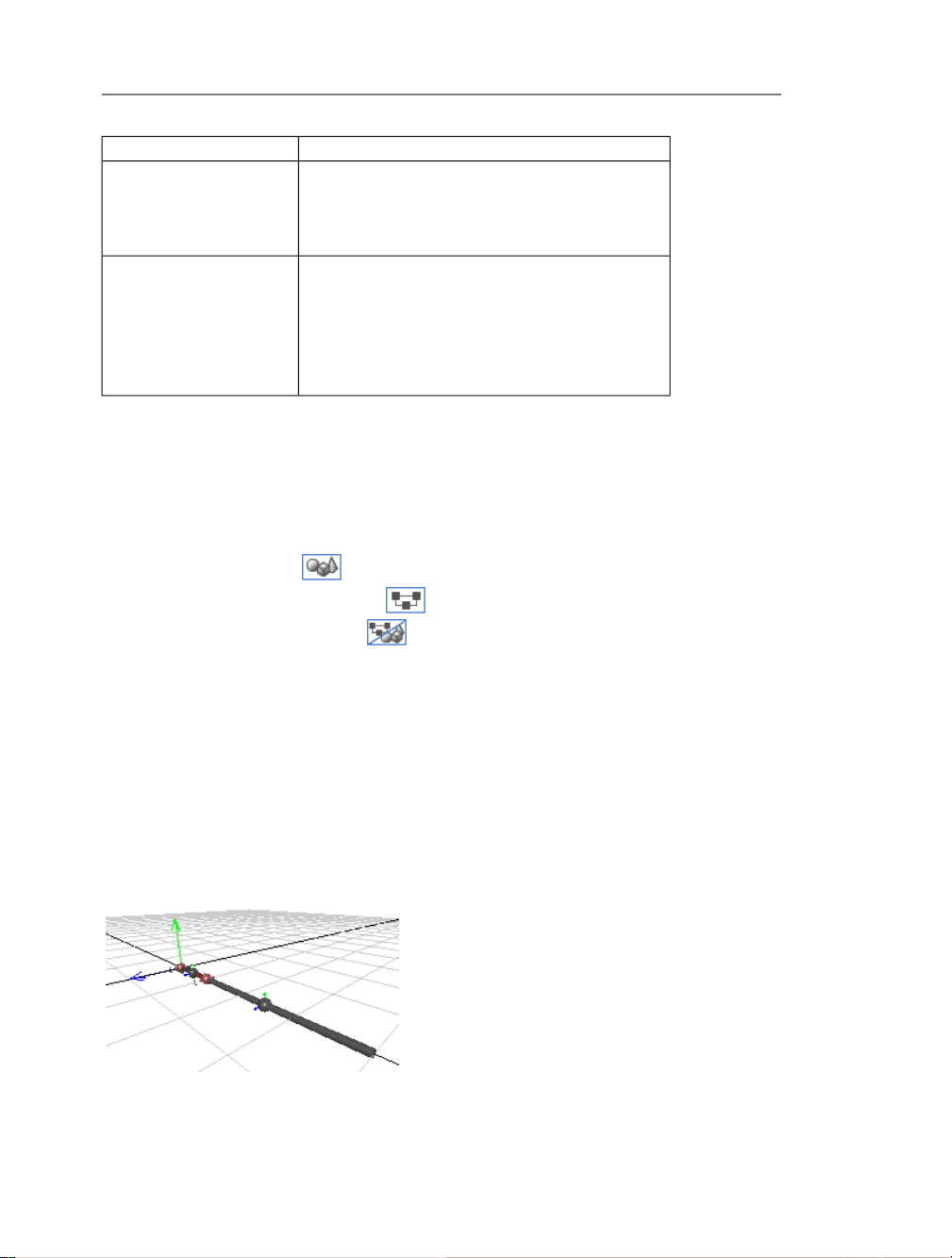
80 • 4 Simulating and Visualizing a Model
DescriptionComponent
Contains tools for hiding and displaying components
2. Main 3-D toolbar
3. Construct mode controls
in the 3-D workspace, toggling between different
modes, selectingcamera navigationtools,and changing
the 3-D model view.
Controls forbuilding andassembling a3-D model,and
connecting 3-D objects. Note: When you switch to
playback mode,the constructmode controlsare hidden
and the playback controls for animating a 3-D model
and specifying camera tracking options are displayed
in this toolbar.
You can hover your mouse pointer over any of the buttons to view their descriptions.
Displaying the 3-D Workspace
To display the 3-D workspace, use the buttons located at the bottom of the MapleSim window. By default, the 3-D workspace is not displayed.
Click the3-D viewbutton ( ) if you wantto workwith yourmodel inthe 3-Dworkspace
only, the block diagram view button ( ) if you want to work in the model workspace
only,or the combined view button( ) if youwant to work in boththe model workspace
and 3-D workspace at the same time.
Viewing and Browsing 3-D Models
In the 3-D workspace, you can view and browse a 3-D model from the perspective view or
one of the orthographic views. The perspective view allows you to examine and browse a
model from all angles in 3-D space. It allows you to see 3-D spatial relationships between
elements inyour model.In theperspective view, objects that are closer to the cameraappear
larger than those that are further away from the camera.
In the following image, a double pendulum model is shown from the perspective view.
Page 91
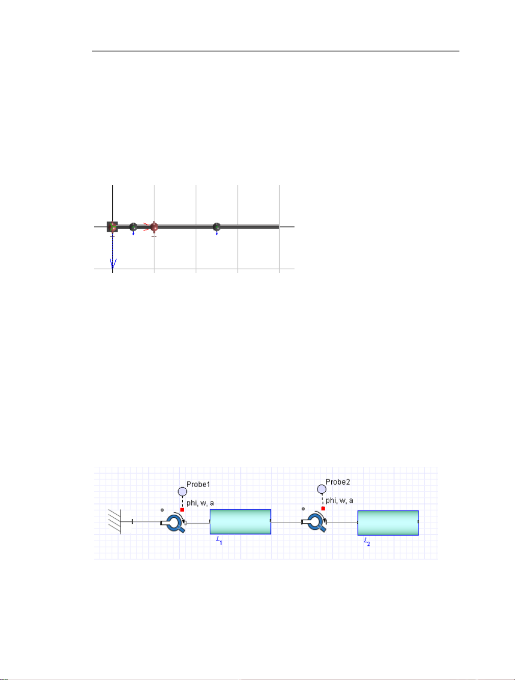
4.7 Visualizing a Multibody Model • 81
You can alsoview your3-D modelfrom front, top, and sideorthographic views.Orthographic
views useparallel projectionas opposedto perspectiveprojection, soyour 3-D model appears
as a attened object because no depth information is shown. Orthographic views are
sometimes referred to as "true length" views because they display undistorted lines and
distances in the view plane that is perpendicular to the objects; these views are useful for
analyzing spatial relationships or clearances between objects.
In the following image, the double pendulum model is shown from the top orthographic
view.
You can browse a model andchange themodel view while an animationis staticor playing.
In all of the views, you can pan and zoom into or out from your model. In the perspective
view, you can also move the camera to view your model from above or below, and from
any direction around your model.
Tip: Before panning,zooming, ormoving thecamera arounda large 3-Dmodel, hoveryour
mouse pointer over the object that you want to focus on. MapleSim adjusts the navigation
controls according to the object on which you place the mouse pointer.
Adding Shapes to a 3-D Model
By default, basic spheres and cylinders called implicit geometry are displayed in the 3-D
workspace to represent physical components in your model. For example, consider thefollowing double pendulum model, which contains two revolute joints and two subsystems
that represent planar links.
Page 92

82 • 4 Simulating and Visualizing a Model
In the 3-D workspace, the implicit geometry of the fully assembled pendulum model is
displayed as follows.
In this example, the spheres represent the revolute joints and rigid bodies, and the cylinders
represent the planar links.
Implicit geometry that is not connected to other implicit geometry is drawn in a light gray
color; implicit geometry that is assembled is drawn in a dark gray color, with the exception
of joint objects, which are drawn in red.
Note: Components that you exclude from a simulation in the model workspace are not
displayed in the 3-D workspace.
If you want to create a more realistic representation of your model, you can add shapes and
lines called attached shapes to your model. To do so, you rst add and connect attached
shape components from the Multibody →Visualization palette to your block diagram in
the model workspace.
When you simulate your model, the attached shapes are displayed in the 3-D workspace,
in addition to the implicit geometry. In the following image, attached shapes have been
added to represent the pendulum stem and bob pictorially. Also, a trace line - the curved
line in the image - is used to depict the locus of points that will be traced by a particular
part of the model during a simulation.
You can customize the color, size, scale, and other visual aspects of the attached shapes by
setting parameter values for individual components in the Inspector tab before simulating
the model.
Page 93
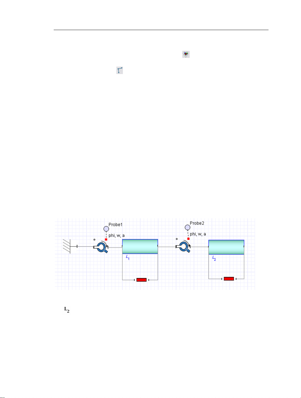
4.7 Visualizing a Multibody Model • 83
If you want to view only the implicit geometry in the 3-D workspace, you can hide the attached shapes by clicking the attached shapes button ( ) in the main 3-D toolbar. If you
want to view the attached shapes only, you can hide the implicit geometry by clicking the
implicit geometry button ( ).
For more information about attached shape components, see the MapleSim Library Ref-
erence → Multibody → Visualization → Overview topic in the MapleSim help system.
Note: If your model contains Flexible Beam components, deection of the beam will not
be depicted in the implicit geometry of your 3-D model.
Example: Adding Attached Shapes to a Double Pendulum Model
In the following example, you willadd cylinder shapesto represent thependulum stem and
a sphere component to represent the pendulum bob. You will also add a Path Trace com-
ponent to display the path on which the revolute joint will move during an animation.
1. In the Libraries tab, expand the Examples palette, expand the Multibody menu, and
then open the Double Pendulum example.
2. Expand the Multibody palette and then expand the Visualization menu.
3. Add two Cylindrical Geometry components below the planar link subsystems in the
model workspace.
4. Connect the components as shown below.
5. From the same menu, add a Spherical Geometry component and place it to the right of
the shared subsystem.
6. Right-click(Control-click for Macintosh) the Spherical Geometry component andselect
Flip Horizontal.
7. Add a Path Trace component and place it between the two Cylindrical Geometry
components.
Page 94
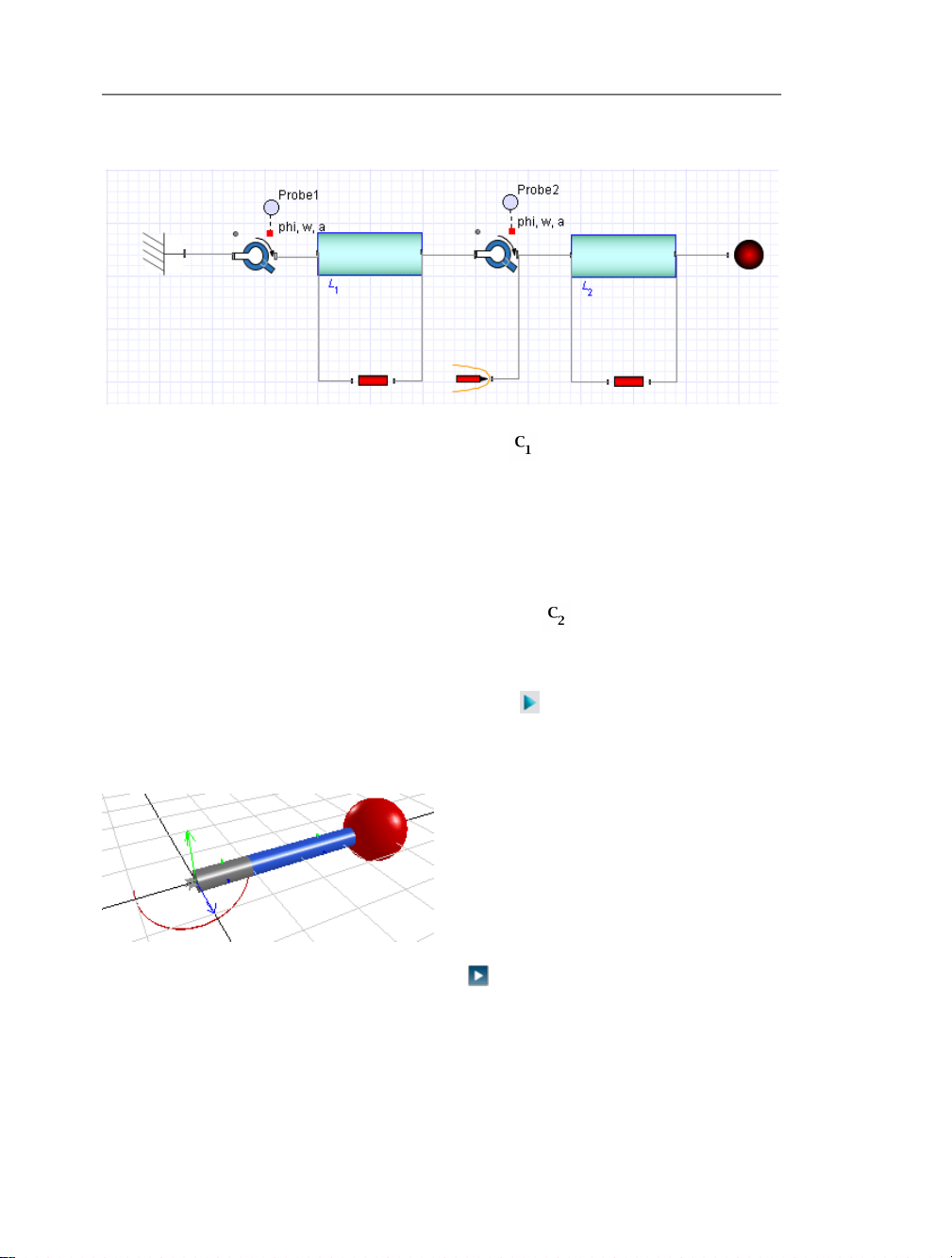
84 • 4 Simulating and Visualizing a Model
8. Connect the components as shown below.
9. Select the rst Cylindrical Geometry component ( ) in the model workspace.
10. In the Inspector tab on the right side of the MapleSim window, change the radius of
the cylinder to 0.3.
11. To select a color for the cylinder, click the box beside the color eld and click one of
the color swatches.
12. Select the second Cylindrical Geometry component ( ) in the model workspace.
13. Change the radius of this cylinder to 0.3 and change the color.
14. To simulate the model, click the simulation button ( ) in the main toolbar.
When the simulation is complete, the 3-D workspace is displayed. The 3-D workspace is
set to playback mode automatically and displays your model with the attached shapes.
15. To animate the model, click the play button ( ) below the 3-D workspace.
Page 95
4.7 Visualizing a Multibody Model • 85
Building a Model in the 3-D Workspace
You can build MapleSim models by adding and connecting objects in the 3-D workspace.
To addcomponents toa 3-Dmodel, youcan dragmultibody componentsfrom theMultibody
palette, the Favorites palette, a custom library that you created, or from the search pane in
the Libraries tab.
You can toggle between construct mode and playback mode to perform specic tasks in
the 3-D workspace. In construct mode, you can add, connect, and lay out 3-D objects, and
set initialconditions for jointsand other multibody components byusing graphical controls
in the 3-D workspace. In playback mode, you can animate your 3-D model and specify
camera tracking options to center an object in the 3-D workspace during an animation.
Any changesthat youmake toyour 3-Dmodel areautomatically shownin the block diagram
representation displayed in the model workspace and vice versa. For example, if you add
and connect a Flexible Beam component in the 3-D workspace, the block diagram representation of the Flexible Beam with the added connection lines will be displayed in the
model workspace at the same time.
Notes:
• Subsystems cannot be created in the 3-D workspace. They must be created in the model
workspace.
• Components from the multibody Forces and Moments, Sensors, and Visualization
component libraries cannot be dragged into the 3-D workspace. You must add these
components in the model workspace.
Moving Objects in the 3-D Workspace
In construct mode, you can position individual objectsor groups of objects by clicking and
dragging the 3-D manipulators in the 3-D workspace.
To display the3-D manipulator for a single unconnected object, click the objectonce in the
3-D workspace.You can then click anddrag the bluearrow of the3-D manipulator to move
the object along the Z axis, the green arrow to move the object along the Y axis, and the
red arrow to move the object along the X axis. You can also click and drag the sphere at
the center of the 3-D manipulator to move the object in all directions.
Page 96

86 • 4 Simulating and Visualizing a Model
For a group of connected objects, the conguration of your model determines where the 3D manipulators are located.
• If your 3-D model contains a Fixed Frame component, click the square that represents
the Fixed Frame component to display the 3-D manipulator.
• If your model does not contain a Fixed Frame component, click the object that denes
the initial conditions for your system to display the 3-D manipulator. For example, if
your model contains a Rigid Body component with its initial condition parameters set
to Strictly Enforce, that Rigid Body component displays the 3-D manipulator. When a
model is moved in the 3-D workspace, the initial conditions are updated for all of the
other Rigid Body components that depend on the Rigid Body component that has its
initial conditions set to Strictly Enforce.
• If your model does not contain a Fixed Frame component or a Rigid Body component
with its initial conditions set to Strictly Enforce, click any of the objects in your 3-D
model to display the 3-D manipulator. When you move the group of objects, the initial
conditions of all of the multibody components in your model are set to Treat as Guess.
• Note: Todisplay 3-Dmanipulators, themultibody componentsin yourmodel mustcontain
numeric parameter values. If custom parameter values dened in a parameter block,
global parameter, or subsystemparameter have been assigned toa multibodycomponent,
no 3-D manipulator will be displayed when you click that component in the 3-D workspace.
Assembling a 3-D Model
To generate a 3-D animation, you must assemble your 3-D model to display its initial conditions inthe 3-D workspace.This step is performed automaticallywhen you simulate your
model; however, for certain models, you can perform this step manually by clicking the 3-
D viewupdate button( ) in constructmode. Byclicking thisbutton, youupdate the initial
conditions and properties of your 3-D model without generating simulation data.
Note: You can only assemble 3-D models with a valid conguration and valid connection
lines. For example, if you attempt to assemble a 3-D model with missing connection lines,
an error message will be displayed in the console pane and no animationwill be generated.
Tip: To show the correct physical conguration of your 3-D model in its initial state, you
may need to assemble your model after you edit model parameters and properties.
Using the Unenforce Constraints Button to Manipulate Joints in the 3-D Workspace
In constructmode, youcan select a joint object in the3-D workspaceand clickthe unenforce
constraints button( )to specify that the kinematicconstraints ofthe jointare notenforced
in the3-D workspaceas you build your model. Joints withunenforced kinematicconstraints
Page 97

4.7 Visualizing a Multibody Model • 87
are displayed in pink in the 3-D workspace and its initial conditions are not shown in the
3-D workspace as you build your model.
You may want to use the unenforce constraints button if, for example, you are creating a
closed-loop modelin the3-D workspaceand you need a jointto remainin aspecic position
as you are building and laying out your 3-D model.
Notes:
• The unenforce constraints button does not affect the actual initial conditions specied
for your joint components in the Inspector tab; it affects the initial conditions depicted
in the 3-D workspace for display purposes only.
• Initial conditions for other joints with enforced kinematic constraints will be shown in
the 3-Dworkspace, butwill notaffect relatedjoints withunenforced kinematicconstraints.
For example, consider a double pendulum 3-D model that contains a revolute joint with
unenforced kinematic constraints and a second revolute joint with enforced kinematic constraints. If you change the initial angle of the joint with enforced kinematic constraints, the
joint with the unenforced kinematic constraints will remain in its original position while
the joint with enforced kinematic constraints will be shown at the new initial angle. To
display all of the new initial conditions in the 3-D workspace, you must assemble your
model by running a simulation or clicking the 3-D view update button ( ).
Displaying Attached Shapes as Your Build a 3-D Model
When youconnect Cylindrical Geometry, TaperedCylinder Geometry, BoxGeometry,
or Spherical Geometry components to your block diagram in the model workspace, the
corresponding attached shapes are displayed in the 3-D workspace in both construct mode
and playback mode.The attachedshape isdisplayed in the3-D workspaceafter you connect
all of its ports to compatible ports of multibody components in the model workspace.
Working with CAD Geometry
CAD geometry can also be displayed in the 3-D workspace in both construct mode and
playback mode. When you add a CAD Geometry component anywhere in the model
workspace, the corresponding CAD image is displayed in the 3-D workspace regardless of
whether the CAD Geometry component is connected to other components in your model.
If a CAD Geometry component is not connected to other components, it will be drawn at
the originof the3-D grid;if aCAD Geometry component is connectedto anothercomponent, it will be drawn at the origin of the coordinate frame of the modeling component to
which it is attached.
You can dene the translational and rotational offset for CAD images either before or after
connecting the corresponding CAD Geometry component to your model. To dene these
Page 98

88 • 4 Simulating and Visualizing a Model
offsets, youcan select theCAD Geometry component inthe model workspaceand specify
parameter values in the Inspector tab.
Example: Building a Double Pendulum Model in the 3-D Workspace
In thisexample, youwill buildand animatea double pendulum model in the 3-Dworkspace.
You will perform the following tasks:
1. Add and move objects in the 3-D workspace.
2. Connect the 3-D objects.
3. Set initial conditions for the joints in your model.
4. Animate the 3-D model.
In a new MapleSim document, the 3-D workspace is set to construct mode by default.
Adding and Moving Objects in the 3-D Workspace
1. Open a new MapleSim document.
2. At the bottomof the MapleSim window, click the 3-D view button ( ) to display the
3-D workspace.
3. In the Libraries tab, expand the Multibody palette and then expand the Bodies and
Frames menu.
4. Fromthe palette,drag aFixed Frame component intothe 3-Dworkspace. Agray square,
which represents the Fixed Frame component, is added to the 3-D workspace and its 3-D
manipulator is displayed.
You can use this manipulator to position objects in the 3-D workspace.
Page 99

4.7 Visualizing a Multibody Model • 89
5. Position the Fixed Frame object at the origin of the grid by clicking anddragging the 3-
D manipulator arrow controls.
6. From the Multibody → Joints and Motions menu, draga Revolute component into the
3-D workspace and place it to the right of the Fixed Frame.
7. Fromthe Multibody→ Bodies and Frames menu, draga RigidBody Frame component
into the 3-D workspace and place it to the right of the Fixed Frame.
8. From the same menu, drag a Rigid Body component into the 3-D workspace and place
it to the right of the Rigid Body Frame.
Page 100

90 • 4 Simulating and Visualizing a Model
Tip: To zoom into and out from the 3-D workspace, rotate your mouse wheel. To pan your
model, hold the Shift key and drag your mouse pointer in the 3-D workspace.
9. Fromthe samemenu, draganother RigidBody Frame component intothe 3-Dworkspace
and placeit tothe right of the RigidBody. Thecomponents for the rst pendulum link have
been added.
10. Repeat steps 7 to 9 to add components for a second pendulum link at the right of the
last Rigid Body Frame component that you added.
Connecting 3-D Objects
You will now connect the objects that you added in the previous task.
1. Click the connect button ( ).
 Loading...