Luminex MasterPlex QT User Manual

Tutorial for MasterPlex QT® v2.5

http://www.MiraiBio.com © 2007 Hitachi Software Engineering America, Ltd. All Rights Reserved.

Table of Contents

Running MasterPlex QT using an existing template .............................................3

Marking and Grouping Wells...............................................................................13

Designating the Standard/Known Concentrations:..............................................21

Select the Standard Curve Model .......................................................................26

Utilizing the Virtual Plate Feature........................................................................30

Analyzing a single QuantigenePlex plate............................................................40

Other Features to Explore...................................................................................45

http://www.miraibio.com 2 MasterPlex QT

Running MasterPlex QT using an existing template

The following exercise will show how to run MasterPlex QT v2.5 using sample data that
are included when the program is installed.

When you start MasterPlex QT v2.5, you will see the plate wizard dialog box:

Click the Next button:

http://www.miraibio.com 3 MasterPlex QT

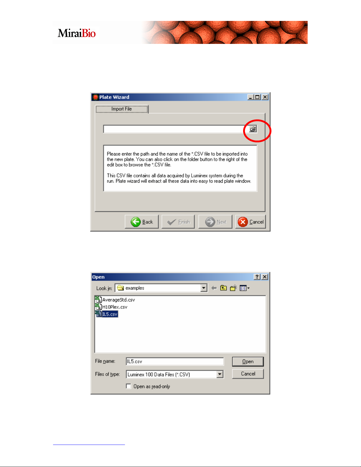
Select the Import a new plate option, and click Next:

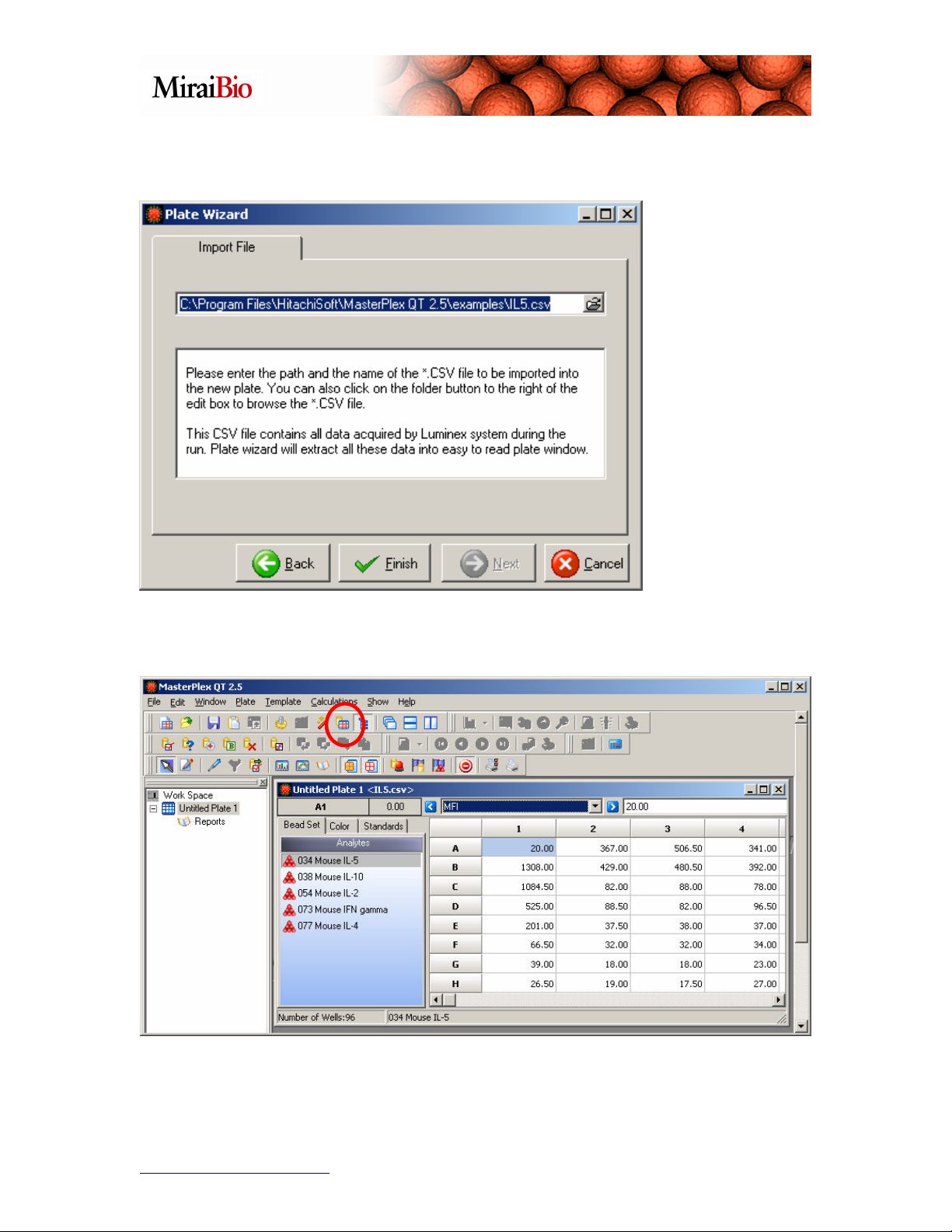
Click on the button with the folder icon to navigate to the .csv file. Navigate to

C:\Program Files\HitachiSoft\MasterPlex QT 2.5\examples, and select the file titled
IL5.csv.

http://www.miraibio.com 4 MasterPlex QT

Next, click the Open button shown above.

Click the Finish button.

Click on the Template Manager icon shown circled above to select the template for this
plate.

http://www.miraibio.com 5 MasterPlex QT

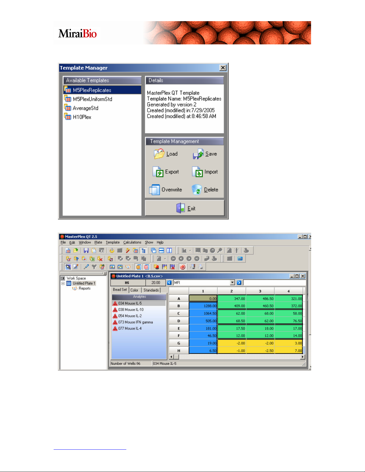
Click on the
M5PlexReplicates
template, and click on
the Load button.

Please note how the wells are color-coded.

• Copper = the background wells.

• Blue = the standard wells.

• Green = the unknown wells.

• Yellow = the (optional) control wells.

http://www.miraibio.com 6 MasterPlex QT

Also note the black borders that show how the wells are grouped. Please note that
MasterPlex QT treats standard wells in a single group differently than background wells,
unknown wells or control wells grouped together in a single group:

• When standard wells are placed in one group, MasterPlex QT will use data from

that group to create a standard curve for each analyte. If you have replicate
standard wells, MasterPlex QT will determine which wells are replicates by
comparing their standard/known concentration values. For replicate standards,
you can choose to calculate the standard curves by either using the average values
for the replicate wells, or by using the individual values.

• When background, unknown or control wells are grouped together, you can

instruct MasterPlex QT to treat each group as a set of replicate wells, and
calculate the mean, standard deviation and %CV for each group when you
calculate your unknown concentrations.

In the above picture, there is one group of standard wells, and there are seven different
standard wells in that group. In this example, there are no replicate standards. There are
three groups of unknown wells, each with 6 replicates, and one group of control wells,
also with six replicates.

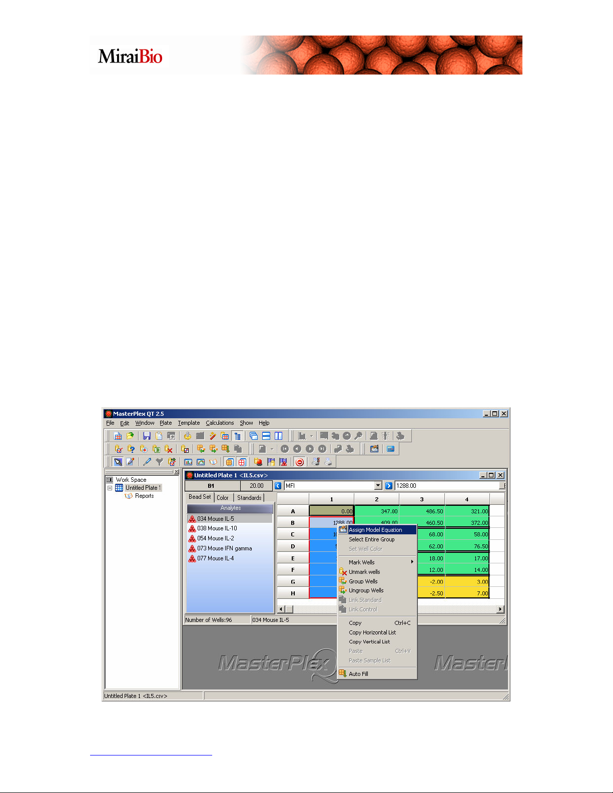
Before we calculate the unknown concentrations, we should select the model equation we
wish to use. To assign the model equation, right-click with your mouse on one of the
wells in the standard group, and select Assign Model Equation, as shown below.

http://www.miraibio.com 7 MasterPlex QT

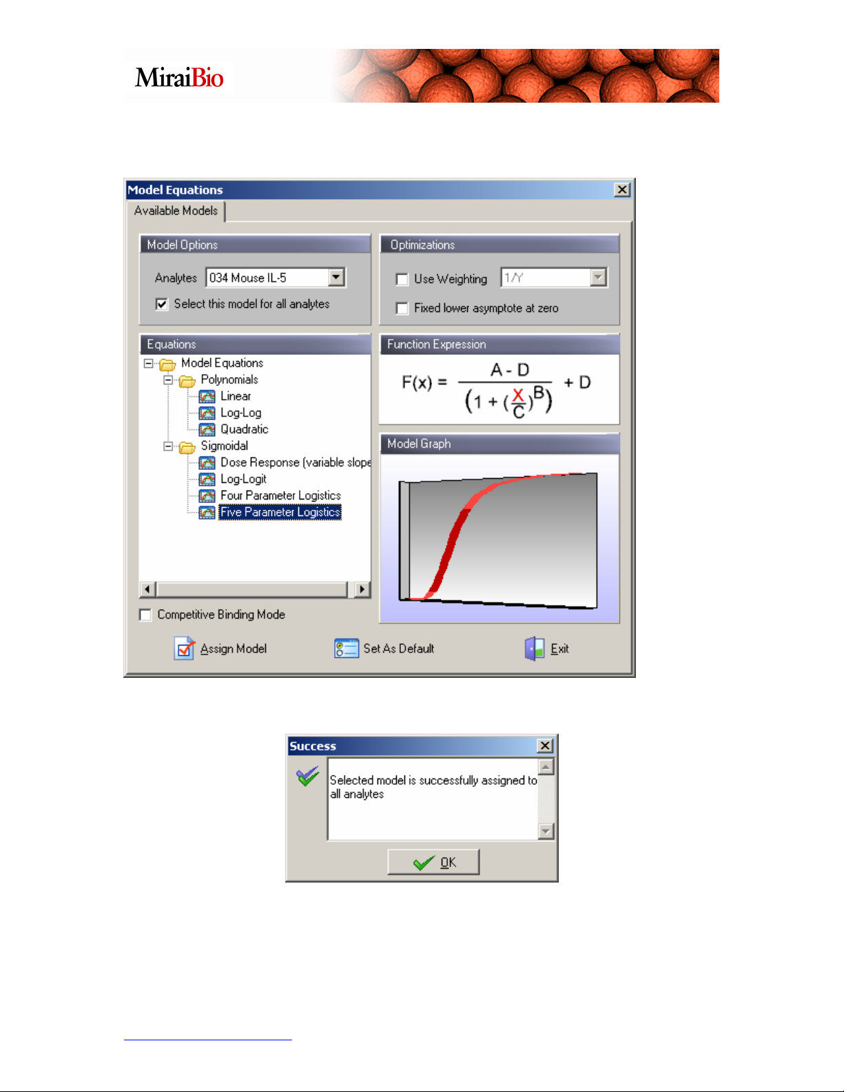
For this example, we will select the Five Parameter Logistics curve model, without
weighting:

Click on Assign Model. The following dialog box will show up:

Click OK.

http://www.miraibio.com 8 MasterPlex QT

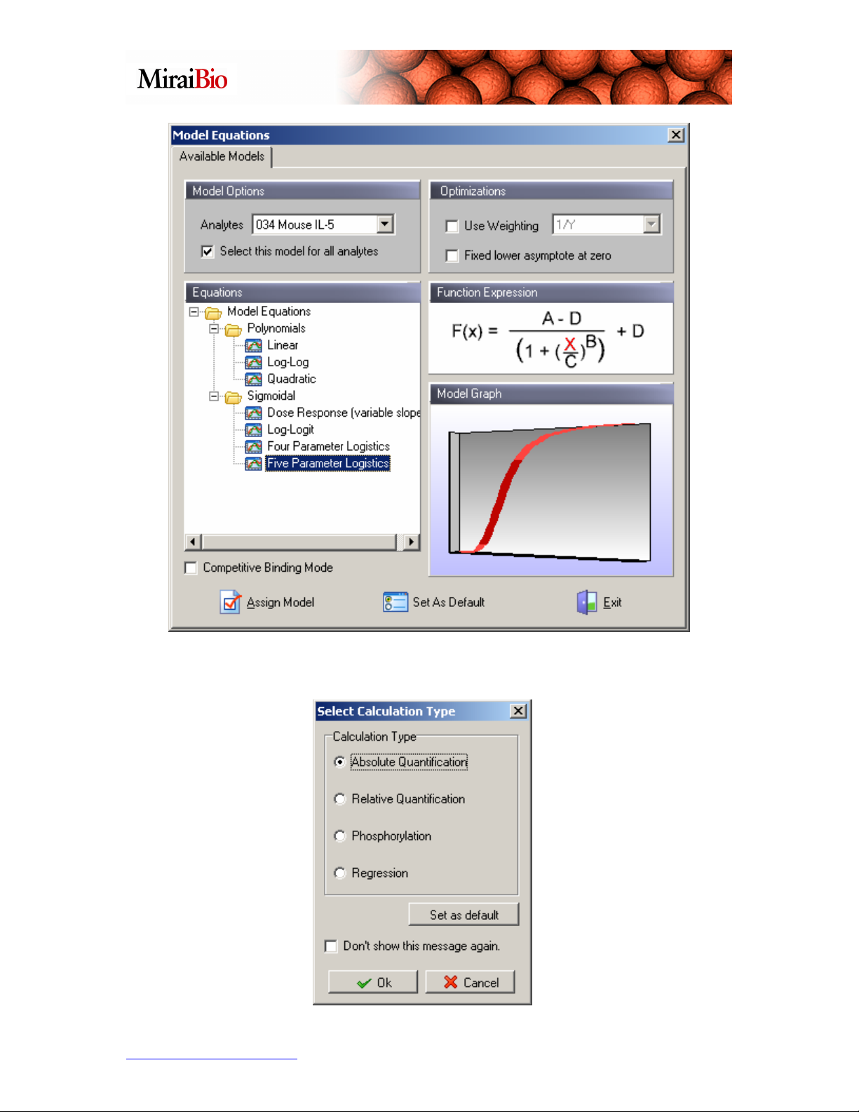
Click Exit to leave the Model Equations dialog box. The following dialog box will then
appear. Select Absolute Quantification, and click OK.

http://www.miraibio.com 9 MasterPlex QT

You will then see the following dialog box:

Now, from the drop-down pick-list, select Concentration/Fold Change.

You can now toggle through the list of analytes on the left and view the concentration
information for each analyte and each well.

http://www.miraibio.com 10 MasterPlex QT

Note for the IL-10 analyte, some of the wells show a value <26.47. If we go to the drop­down pick-list, and select Standard/Independent Values, we see that the lowest known
standard concentration for this analyte is 26.47.

So, what does <26.47 mean here? For 4-parameter logistic and 5-parameter logistic
curve models, when the best-fit curve is generated based on the data, there is a lower
limit for the Median Fluorescent Intensity (MFI) values that the model can use to
calculate an estimated concentration for a sample. When a sample has an analyte whose
MFI value is below this lower limit, the model cannot be used to calculate the estimated
concentration. However, if the MFI value for an analyte is below the MFI value for the

http://www.miraibio.com 11 MasterPlex QT

lowest point on the standard curve, we can infer that the concentration for that analyte is
less than the concentration of the lowest point on the standard curve for that analyte. So,
in the example above, we cannot use the model to calculate an estimated concentration,
but we can infer that the concentration is less than 26.47 pg/mL. There is a similar upper
limit on the 4-parameter logistic and 5-parameter logistic curve models, with an
analogous “>” nomenclature when the MFI value is above the upper limit of the curve
model, but we can infer the concentration is above the highest point on the standard curve
for that analyte.

For many users, it is enough to know that we can infer “the concentration is below the
lowest point on the standard curve” or “the concentration is above the highest point on
the standard curve” when we measure a data point outside the range of the model curve.
If you would like additional details on this, please go to the www.MiraiBio.com website.
The presentation The Calculations at the link shown below provides a much more in­depth look at these issues:

http://www.MiraiBio.com/online-demo/online-demos.html

Going back to the exercise, in the plate above, if you wanted to save your work at this
point, you would select File → Save.

Note: When we read in a .csv file from the Luminex machine into MasterPlex QT,
the .csv file does not get altered. When we save the work we’ve done in MasterPlex QT,
it gets saved as an .mlx project file, leaving the original .csv file unaltered.

http://www.miraibio.com 12 MasterPlex QT

Marking and Grouping Wells

We’ll open the IL5.csv plate again, but this time, instead of using a template, we’ll mark
the wells and enter the standard concentrations manually.

Go ahead and close the plate we were working on in the above tutorial by clicking on the
X in the top right-hand corner of the plate window:

Now, click on the New icon to read in a .csv file produced by the Luminex machine
(Note: If you are using build 163 or above, the New icon will not be present. In that case,
please click on the Open icon):

http://www.miraibio.com 13 MasterPlex QT

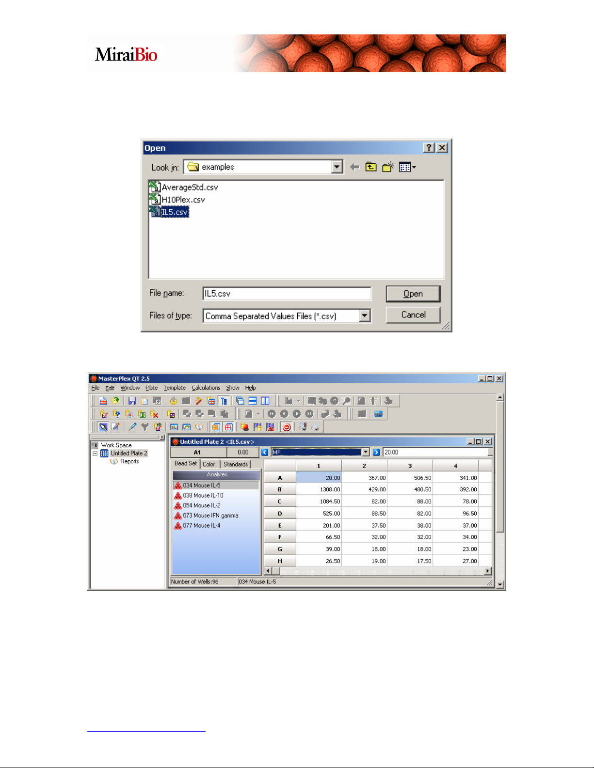
Navigate to C:\Program Files\HitachiSoft\MasterPlex QT 2.5\examples, and select the
file titled IL5.csv.

You will see the window shown below:

This is the same plate we worked with before. If we did not have a template for this plate,
we would need to mark the wells (as shown below).

To mark wells, you highlight them, then right-click, and select how you want to mark
them.

http://www.miraibio.com 14 MasterPlex QT

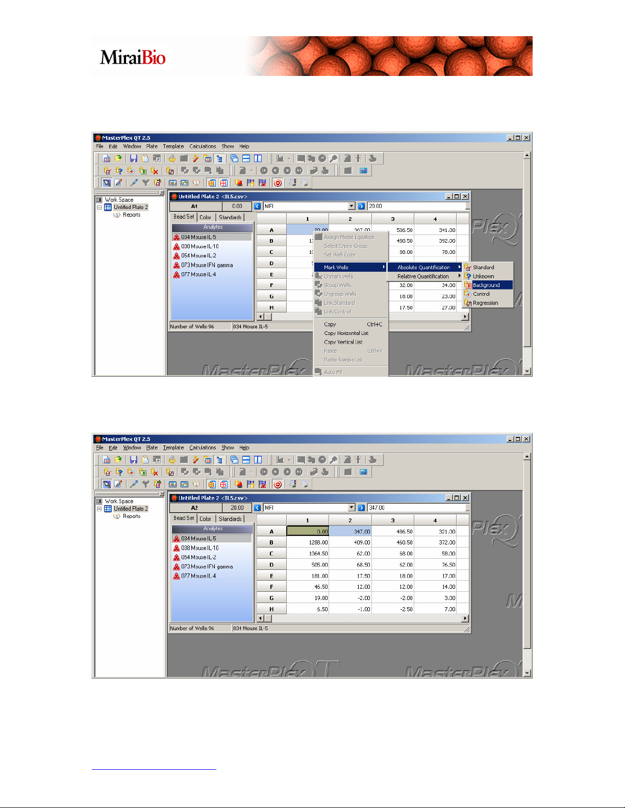
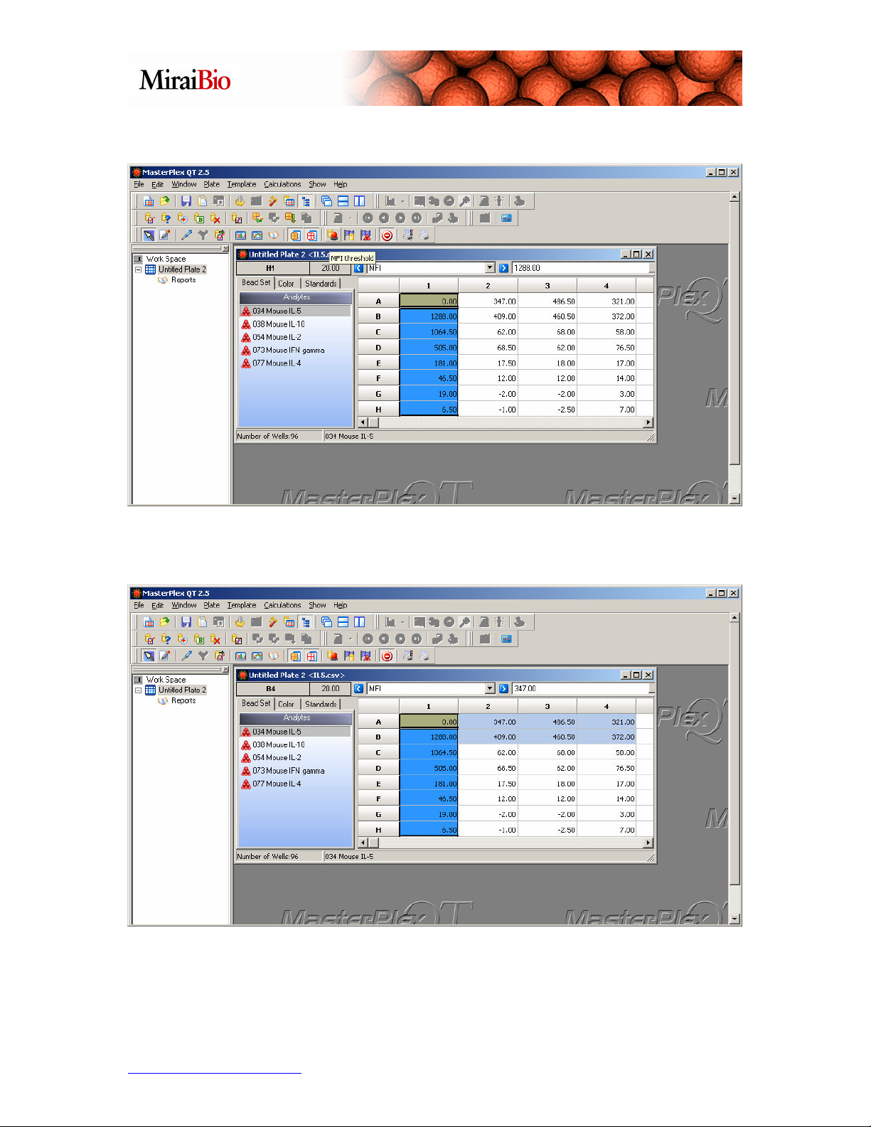
We’ll mark A1 as background: Highlight the well, then right-click, and from the menu,
select Mark Wells → Absolute Quantification → Background.

The well will change color to copper (you may have to click on another well to change
the highlighting to see the copper color indicating a background well).

http://www.miraibio.com 15 MasterPlex QT

Now we will highlight B1 to H1, and mark them as Standard wells:

Now right-click on the wells, and select Mark Wells → Absolute Quantification →
Standards.

http://www.miraibio.com 16 MasterPlex QT

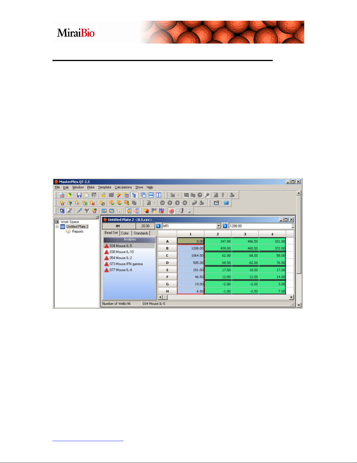
The Standard wells will be grouped together and colored light blue:

Now we’ll highlight A2, A3, A4, B2, B3 and B4, and mark them as a group of Unknown
wells:

http://www.miraibio.com 17 MasterPlex QT

Now right-click on the wells, and select Mark Wells → Absolute Quantification →
Unknowns.

The Unknown wells will be grouped together, and colored green:

Note: Automatic grouping can be turned on or off by going to File → Preferences, and
checking or unchecking Automatic Well Grouping.

http://www.miraibio.com 18 MasterPlex QT

We can repeat this for the group C2, C3, C4, D2, D3, and D4. Highlight those six wells:

Right-click on them, and designate them as Unknown:

http://www.miraibio.com 19 MasterPlex QT

Repeat this for groups E2, E3, E4, F2, F3, F4 and G2, G3, G4, H2, H3, H4.

http://www.miraibio.com 20 MasterPlex QT

Designating the Standard/Known Concentrations:

We can now add the known concentrations for each analyte in the standard wells. The
starting concentrations for each analyte are as follows:

• IL-5 = 15,900 pg/mL

• IL-10 = 19,300 pg/mL

• IL-2 = 20,400 pg/mL

• IFN gamma = 5200 pg/mL

• IL-4 = 21,200 pg/mL

The dilutions are 1:3. We can use the Auto fill feature in MasterPlex QT to quickly enter
in the standard concentration values. First, highlight the standard wells you wish to use
auto-fill for to enter in the standard values.

http://www.miraibio.com 21 MasterPlex QT

Next, right-click on the highlighted group, and select Auto fill from the menu.

The Auto fill dialog box will appear:

http://www.miraibio.com 22 MasterPlex QT

For analyte IL-5, the starting concentration is 15,900 pg/mL, and the dilution factor is 3
(since it is a 1:3 dilution). Note the various arrow keys – these are used to indicate the
direction of the dilution; that is, the direction you would move as if you were doing the
serial dilution in a 96-well plate, moving from most concentrated to least concentrated.
The blue arrows and the red arrows allow you to specify the direction if the dilution spans
more than one column or one row, respectively. The green arrows are used if your
standards lie entirely in either one row or one column. The most concentrated well is B1,
and the serial dilutions proceed down to H1, so we’ll select the green down-arrow key.
For IL-5, the window should appear as shown:

Click Fill, and the following dialog box will appear:

Click OK, and then click Cancel/Exit in the Auto Fill dialog box.

http://www.miraibio.com 23 MasterPlex QT

Now go back to the plate view, and select Standard/Independent Values from the pull­down pick-list.

Now you can see the standard concentrations for IL-5.

http://www.miraibio.com 24 MasterPlex QT

Note if you click on a different analyte, those standard concentration values are still zero.

You will need to repeat this procedure for each analyte. Note that some kit
manufacturers use the same starting concentration for all of the analytes in an assay. In
this case, you can select in the Auto Fill dialog box the Fill in for all bead sets option,
and it will use that starting concentration for all the analytes. For this exercise, please fill
in the starting concentration for each analyte before proceeding:

• IL-10 = 19,300 pg/mL

• IL-2 = 20,400 pg/mL

• IFN gamma = 5200 pg/mL

• IL-4 = 21,200 pg/mL

You can confirm the standard values by selecting Standard/Independent Values from
the pull-down pick-list, then clicking on each bead region in the Analytes list.

http://www.miraibio.com 25 MasterPlex QT

Select the Standard Curve Model

Now we need to select the standard curve model to be used with each analyte. As we did
before, we’ll use the 5-parameter logistic curve model.

Right-click on one of the wells in your standard group, and select Assign Model
Equation from the menu.

http://www.miraibio.com 26 MasterPlex QT

Select Five Parameter Logistics for the model, and check Select this model for all
analytes.

Now click on Assign Model, and click OK in the confirmation dialog box:

http://www.miraibio.com 27 MasterPlex QT

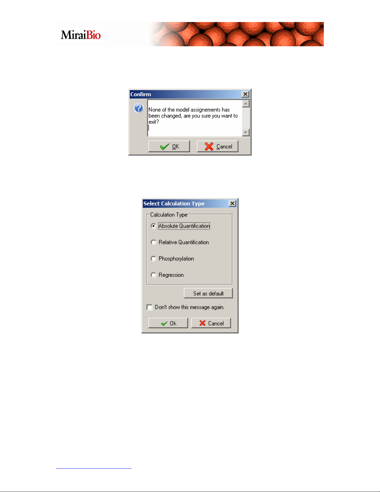
Now click Exit in the Model Equations dialog box. (If you see the following message:
it just means that the choices you made here correspond to the default model assignment.
Click OK.)

The Select Calculation Type dialog box will appear. Select Absolute Quantification
and click OK.

At this point, you can click OK to perform the concentration calculations, as was done
earlier in this tutorial.

http://www.miraibio.com 28 MasterPlex QT

If you wanted to save this information in a template to apply to identical assays in the
future, you will need to open the Template Manager:

From here, you can click on Save, give the template a name, and save it for future use.

http://www.miraibio.com 29 MasterPlex QT

Utilizing the Virtual Plate Feature

The Virtual Plate feature allows you to combine data from multiple plate runs, perform
cross-plate comparisons or expand the data analysis paradigm beyond the current 100
analyte per sample limit of the xMAP technology. The Virtual Plate feature also allows
a researcher to combine the disparate data sets for a single patient sample.

For this tutorial, we will stitch together 2 plates into one virtual plate. To follow along
with this tutorial, you will need 3 sample files. You can download the sample files from

www.MiraiBio.com/downloads.html. Select MasterPlex Suite -> MasterPlex QT ->

MasterPlex QT Documents and download:

1) MasterPlex QT Sample1 file for Virtual Plate Tutorial

2) MasterPlex QT Sample2 file for Virtual Plate Tutorial

3) MasterPlex QT Sample3 file for Virtual Plate Tutorial

After you have downloaded them, please import Sample1 and Sample2 into MasterPlex
QT.

http://www.miraibio.com 30 MasterPlex QT

To open a Virtual Plate, please click on the Plate wizard icon.

The Plate Wizard dialog will pop up.

Click Next.

Select the A virtual plate radio
button and click Next.

http://www.miraibio.com 31 MasterPlex QT

A new empty Virtual Plate will appear.

This dialog screen allows a
user to define the size of the
Virtual Plate they want to use.
For this example, we will use
the default size of 8 Rows and

12 Columns. Please click
Finish.

http://www.miraibio.com 32 MasterPlex QT

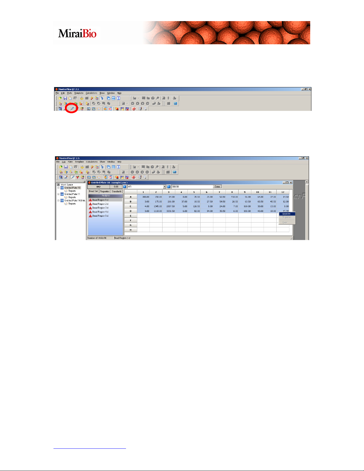
Now, we are ready to merge our 2 sample files together. To begin, please click on the
Virtual Pipette Tool.

This handy tool will allow you to select, aspirate, and dispense the wells you would like
to transfer. Highlight all the wells from the first sample file, right-click, and select
Aspirate.

http://www.miraibio.com 33 MasterPlex QT

To dispense the wells, highlight well A1 in the Virtual Plate, right-click and select
Dispense. Note that the well you choose to dispense into will represent the upper-left
most well from the selection of wells that you aspirated from.

http://www.miraibio.com 34 MasterPlex QT

The Virtual Plate should now contain the data that is in the original sample file.

http://www.miraibio.com 35 MasterPlex QT

Now, let’s do the same thing with the second sample file. Highlight all the wells from
the first sample file, right-click, and select Aspirate.

http://www.miraibio.com 36 MasterPlex QT

Highlight well E1 in the Virtual Plate, right-click and select Dispense.

Note: If the number of bead regions and the bead region names are identical, MasterPlex
QT will automatically map the names together in the Virtual Plate.

The next example will show how to merge 2 plates with different bead region names
and/or a different number of bead regions. Close all the existing plate files and load
Sample1 and Sample3. Open a new Virtual Plate via the Plate Wizard. Transfer the
wells from the Sample1 file just like in the previous example into well A1 of the new
Virtual Plate.

Click on the Analytes filter tool. This tool will assist you in managing and adding
additional bead regions to a well that is already populated.

http://www.miraibio.com 37 MasterPlex QT

Now, select and aspirate all the wells from Sample3. Right-click on well A1 in the
Virtual Plate where you have your well from the first sample file and select Dispense.
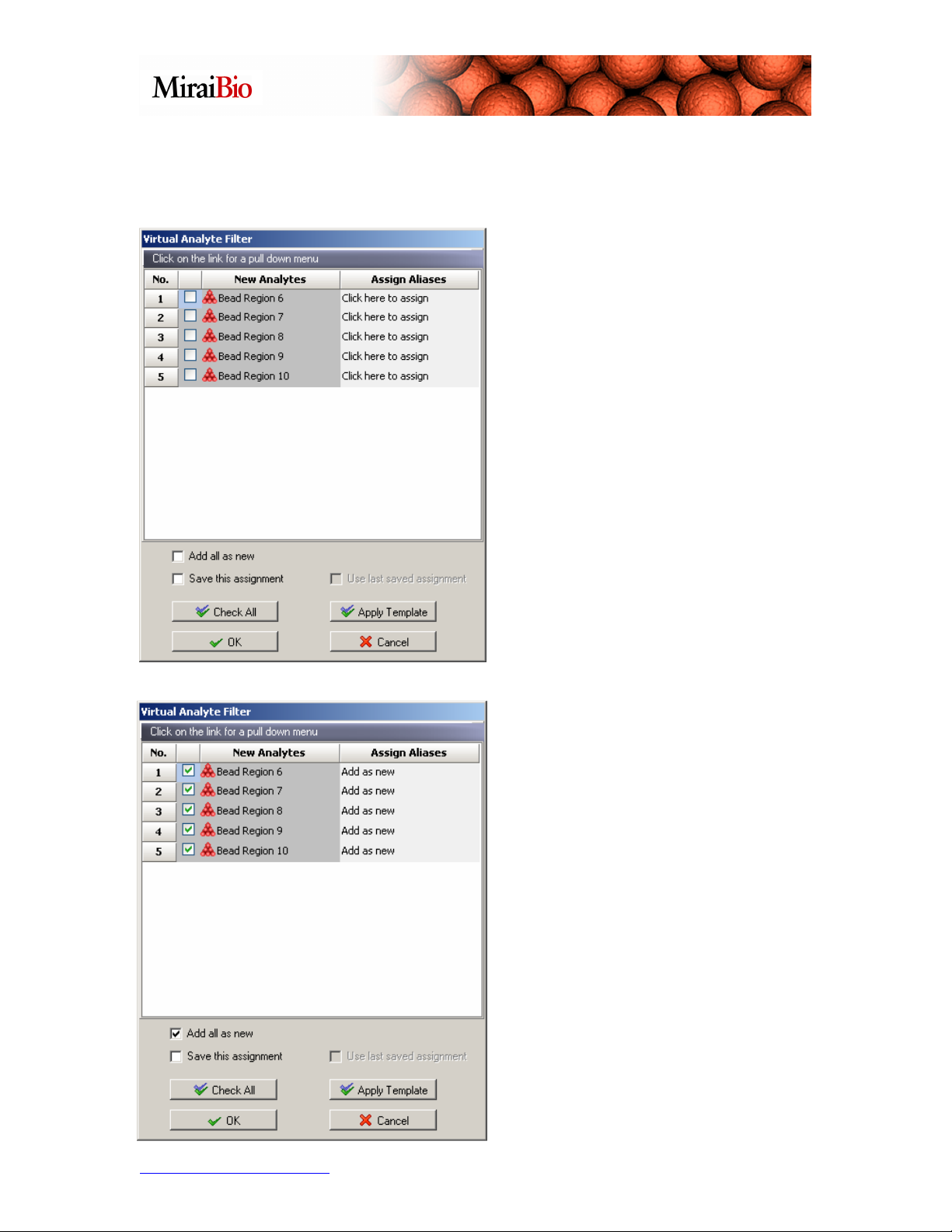
The Virtual Analyte Filter window will pop up.

The New Analytes column lists the
bead regions that you are trying to
pipette into the Virtual Plate. The
Assign Aliases column lists the bead
regions that are already present in the
well that you would like to map to.
MasterPlex QT will automatically
recognize bead regions with identical
names

In our case, we would like to add these
bead regions as new regions in the
existing wells. To do this, check the

Add all as new box and click on
Check All. We have now instructed

MasterPlex QT to add all of our bead
regions to the existing well as new bead
regions. Please click OK.

http://www.miraibio.com 38 MasterPlex QT

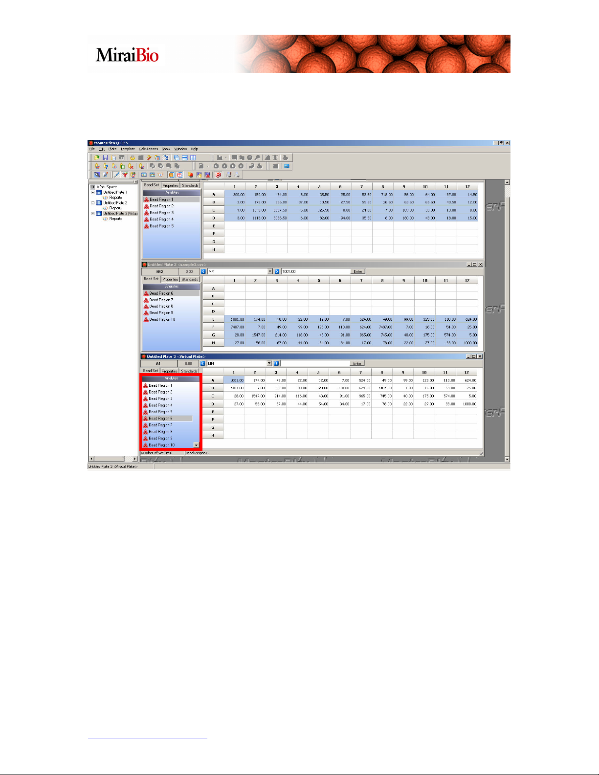
The Virtual Plate now has all 10 bead regions merged together from the original 2 plate
files.

The Virtual Plate feature is a powerful and flexible tool that allows users to perform
cross-plate analyses.

http://www.miraibio.com 39 MasterPlex QT

Analyzing a single QuantigenePlex plate

Note: This can also apply to similar one-plate relative quantification assays.

1. Open Plate: After launching MasterPlex QT, open the data file by clicking the Open
icon or using File  Open Plate.

2. Selecting bead regions that will be used for normalization: Right-click on the bead

region that will be used to normalize the data with. Select Housekeeping. Repeat this
step for all the bead regions that will be used for normalizing the data.

Note: To unselect a panel, right-click on it and select Target

http://www.miraibio.com 40 MasterPlex QT

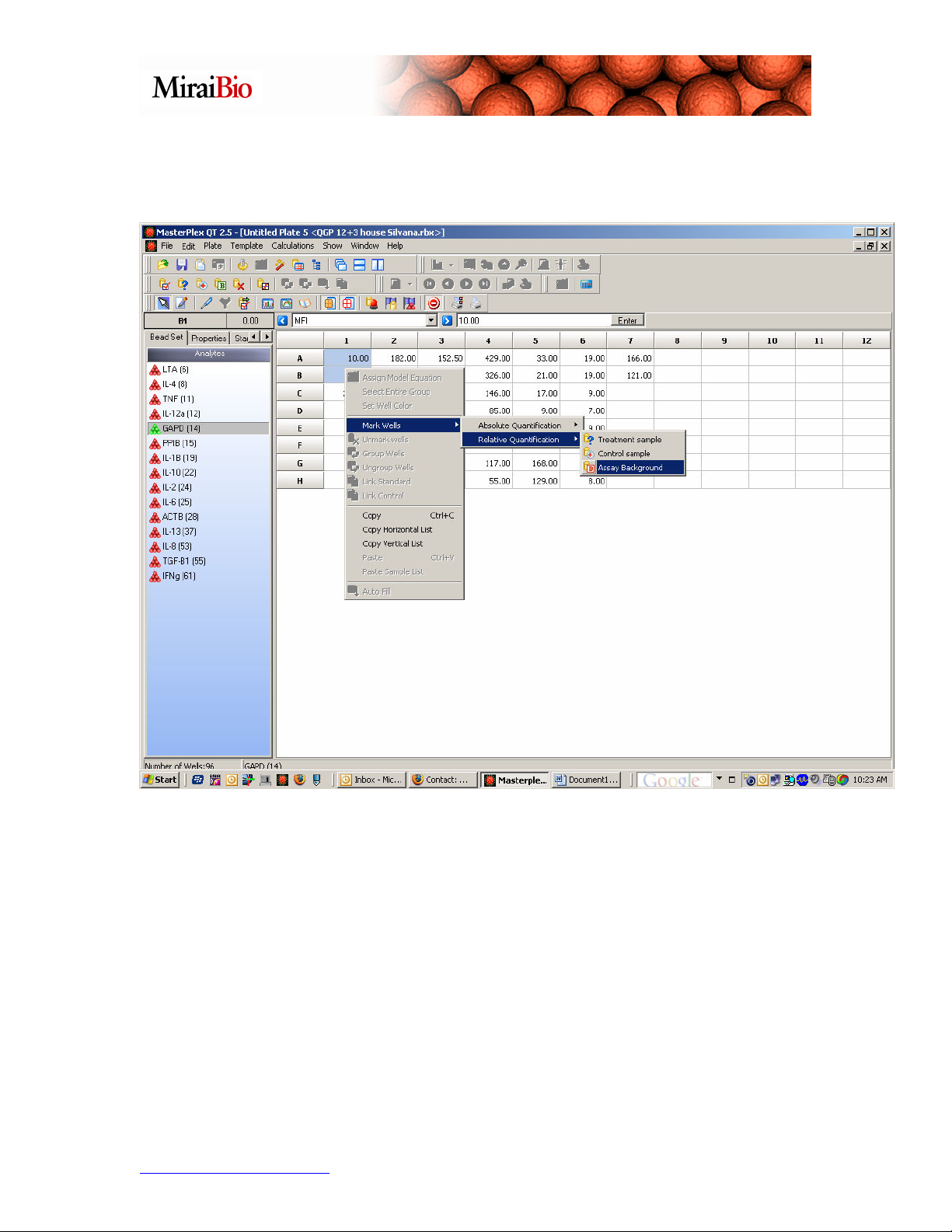
3. Designate well types: Select a well or group of wells and right-click. Navigate to the
Relative Quantification submenu and select the appropriate well type: Assay
Background, Control or Treatment. Repeat for all well types.

http://www.miraibio.com 41 MasterPlex QT

4. Calculate results: Click the Calculate icon and choose 1 of the 3 available Relative
Quantification analysis functions:

http://www.miraibio.com 42 MasterPlex QT

a. Fold Change – This only will calculate the ratio between the Control and

Treatment groups WITHOUT any data normalization.

http://www.miraibio.com 43 MasterPlex QT

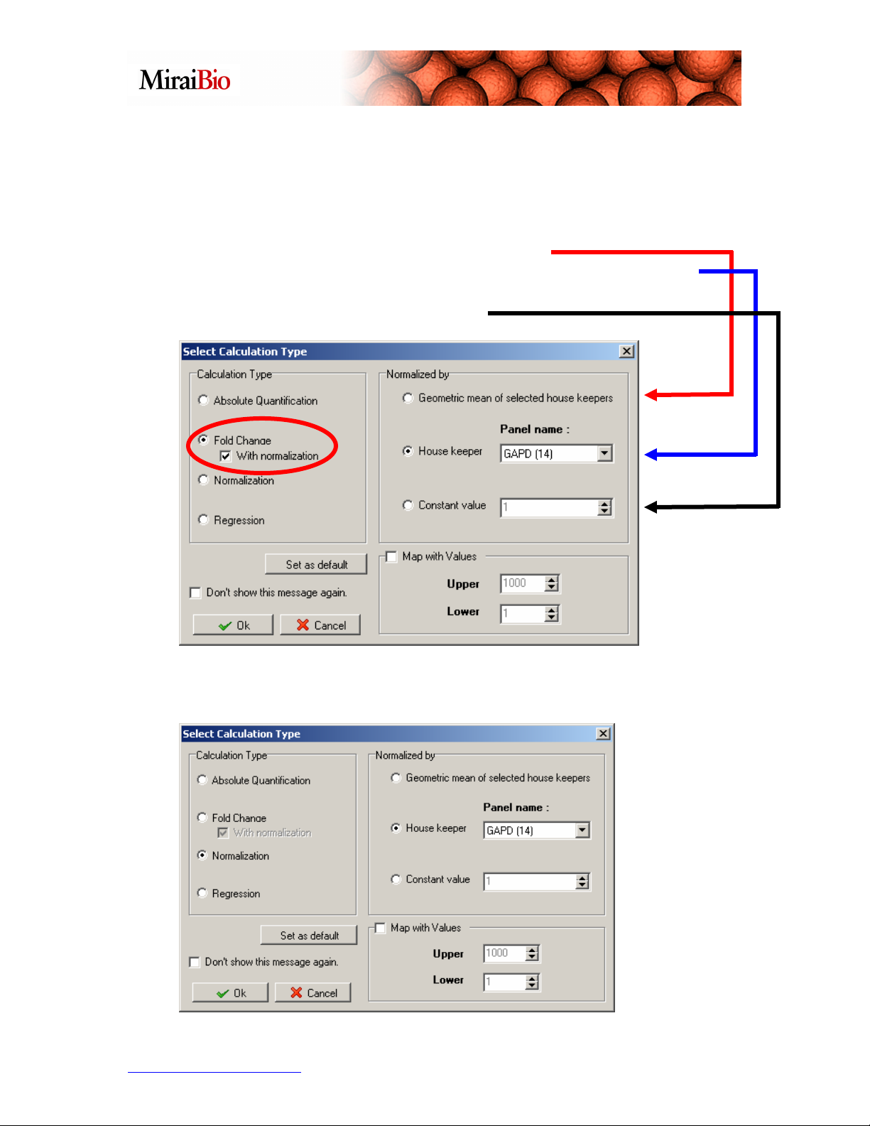
b. Fold Change – If the With normalization check box is ticked, it will perform
a normalization step before the fold change calculation between the treatment and
control groups.

You have 3 options when normalizing:

1. Normalize by a single house keeping gene.

2. Normalize by the geometric mean of all the housekeeping genes
selected in Step 1 if 2 or more genes were selected.

3. Normalized by a Constant value.

c. Normalization – This performs the data normalization step only using one of
the 3 options discussed above.

http://www.miraibio.com 44 MasterPlex QT

Other Features to Explore

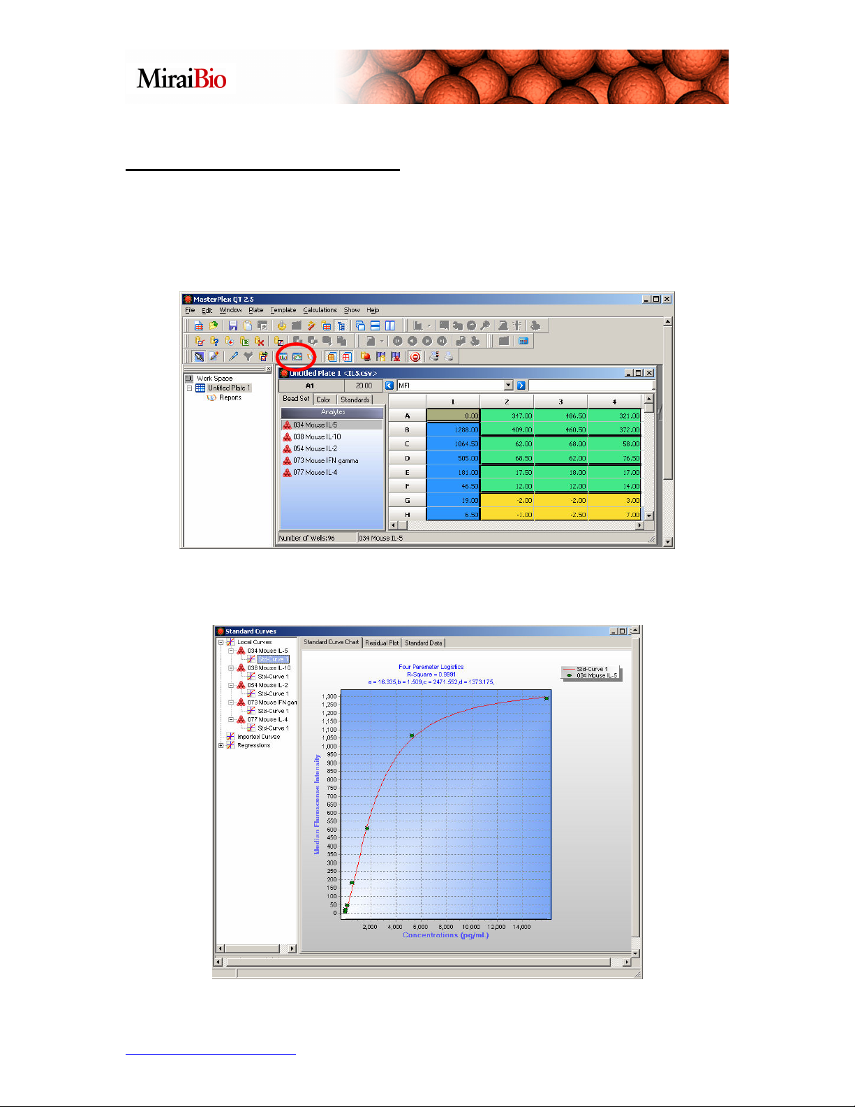
Another thing to explore is the Standard Curve Chart feature, which allows you to
view your standard curves for each analyte. Click on the Open Standard Curves Chart
button shown below.

You can view the standard curve for each analyte.

http://www.miraibio.com 45 MasterPlex QT

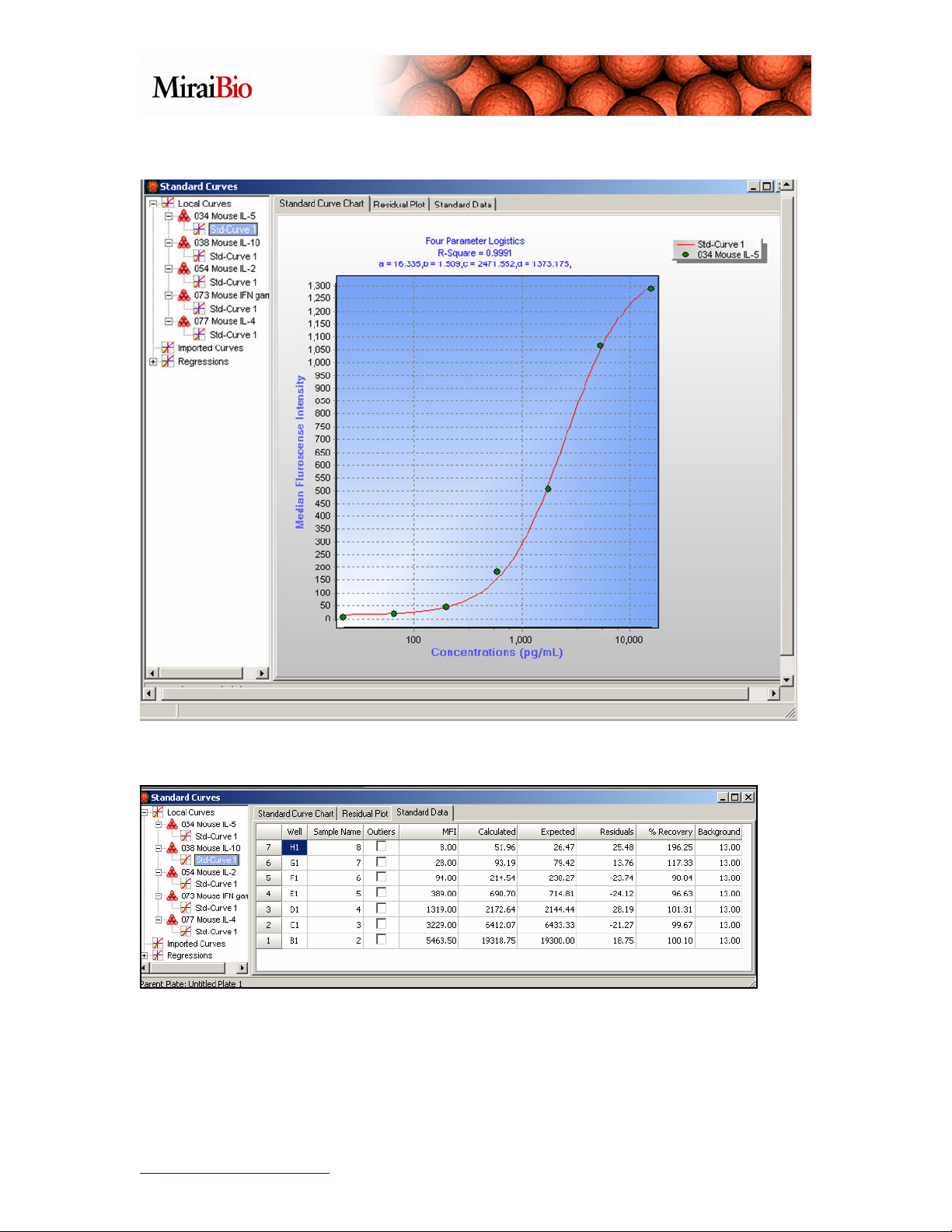
You can right-click on the chart, and select Set X-axis to log scale if you prefer this view.

Click on the Standard Data tab.

http://www.miraibio.com 46 MasterPlex QT

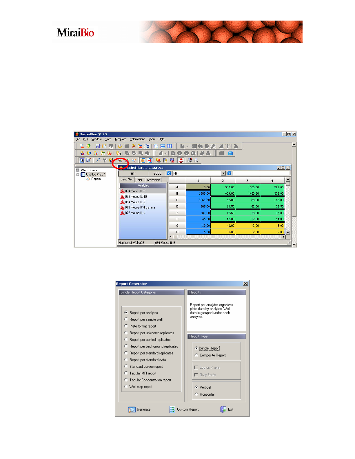
You can see Calculated, Expected, Residual, % Recovery and Background values for
each analyte in each standard well. Also note that if you have outlier points here, you can
designate them, so that they are ignored when you generate your standard curve.

Another feature to explore is the Report Generator. After you have decided on which
curve models you wish to use and performed the necessary calculations, you can click on
the Report Generator icon shown below.

The Report Generator function will appear (Please note that if you are using build 163
or above this window will look slightly different).

http://www.miraibio.com 47 MasterPlex QT

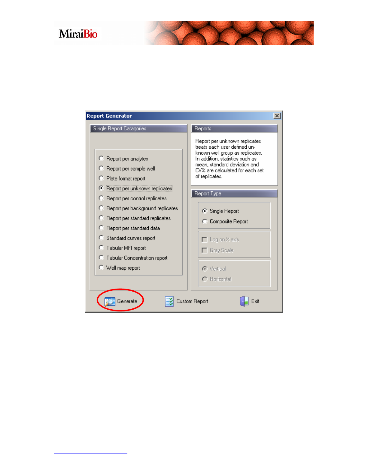
We’ll look at the Report per Unknown Replicates. Recall how grouping some
unknown wells into a single group meant that you were designating those wells as
replicate unknowns. Using the Report per Unknown Replicates, you can now view the

mean, standard deviation and %CV for each group. Select the Report per Unknown
Replicates option above, and click on the Generate button:

http://www.miraibio.com 48 MasterPlex QT

You will see the following report:

http://www.miraibio.com 49 MasterPlex QT

Note that you can then go to the Report menu and click on Save Report.

You will then be presented with a number of options for saving the report (including
PDF, HTML, text, and CSV [for Excel]).

This Tutorial Guide just highlights some of the features of MasterPlex QT v2.5.
Additional features can be found in the on-line manual by going to the Help menu in
MasterPlex QT and selecting the Help option.

On-line demonstrations can be found at:

http://www.miraibio.com/online-demo/online-demos.html

Two demos to note are:

• The Basics, which highlights the basic features of MasterPlex QT.

• The Calculations, which gives a more in-depth view of how the calculations are

performed in MasterPlex QT.

http://www.miraibio.com 50 MasterPlex QT

You can also contact MiraiBio with any questions you have at [phone] (USA
phone number) or by sending an email to [e-mail].

MiraiBio

A Group of Hitachi Software

601 Gateway Blvd.
Suite 100
South San Francisco, CA 94080

Telephone

1.800.624.6176

1.650.615.7600
Facsimile

1.650.615.7639

Trademark Acknowledgments

MasterPlex is a trademark of Hitachi Software Engineering Co., Ltd. Luminex® is a registered trademark
of the Luminex Corporation. All other company and product names mentioned in this manual are
trademarks or registered trademarks of their owners.

© 2007 Hitachi Software Engineering America, Ltd. All Rights Reserved.

http://www.miraibio.com 51 MasterPlex QT