

LeCroy WavePro 7 Zi, DDA 7 Zi, SDA 7 Zi, WavePro DDA 7 Zi, WavePro SDA 7 Zi Operator's Manual
Page 1
Operator’s
Manual
WavePro, ® SDA, and DDA
7 Zi Series Oscilloscopes
Page 2
LRRH
HUDRUDD
Page 3

LeCroy Corporation
700 Chestnut Ridge Road
Chestnut Ridge, NY, 10977-6499
Tel: (845) 578-6020, Fax: (845) 578 5985
Warranty
NOTE: THE WARRANTY BELOW REPLACES ALL OTHER WARRANTIES, EXPRESSED OR IMPLIED, INCLUDING BUT NOT LIMITED TO ANY IMPLIED WARRANTY OF
MERCHANTABILITY, FITNESS, OR ADEQUACY FOR ANY PARTICULAR PURPOSE OR USE. LECROY SHALL NOT BE LIABLE FOR ANY SPECIAL, INCIDENTAL, OR
CONSEQUENTIAL DAMAGES, WHETHER IN CONTRACT OR OTHERWISE. THE CUSTOMER IS RESPONSIBLE FOR THE TRANSPORTATION AND INSURANCE
CHARGES FOR THE RETURN OF PRODUCTS TO THE SERVICE FACILITY. LECROY WILL RETURN ALL PRODUCTS UNDER WARRANTY WITH TRANSPORT
PREPAID.
The oscilloscope is warranted for normal use and operation, within specifications, for a period of three years from shipment. LeCroy will either repair or, at our option, replace
any product returned to one of our authorized service centers within this period. However, in order to do this we must first examine the product and find that it is defective due to
workmanship or materials and not due to misuse, neglect, accident, or abnormal conditions or operation.
LeCroy shall not be responsible for any defect, damage, or failure caused by any of the following: a) attempted repairs or installations by personnel other than LeCroy
representatives or b) improper connection to incompatible equipment, or c) for any damage or malfunction caused by the use of non-LeCroy supplies. Furthermore, LeCroy shall
not be obligated to service a product that has been modified or integrated where the modification or integration increases the task duration or difficulty of servicing the
oscilloscope. Spare and replacement parts, and repairs, all have a 90-day warranty.
The oscilloscope’s firmware has been thoroughly tested and is presumed to be functional. Nevertheless, it is supplied without warranty of any kind covering detailed
performance. Products not made by LeCroy are covered solely by the warranty of the original equipment manufacturer.
Internet: www.lecroy.com
© 2008
by LeCroy Corporation. All rights reserved.
LeCroy, ActiveDSO, JitterTrack, WavePro, WaveMaster, WaveSurfer, WaveLink, WaveExpert, Waverunner, and WaveAce are
registered trademarks of LeCroy Corporation. Other product or brand names are trademarks or requested trademarks of their
respective holders. Information in this publication supersedes all earlier versions. Specifications are subject to change without
notice.
This electronic product is subject to disposal and
Manufactured under an ISO 9000
Registered Quality Management
System.
Visit www.lecroy.com to view the
certificate.
recycling regulations that vary by country and region.
Many countries prohibit the disposal of waste electronic
equipment in standard waste receptacles.
For more information about proper disposal and recycling
of your LeCroy product, please visit
www.lecroy.com/recycle
.
916494 RevA
Page 4

Getting Started Manual
TABLE OF CONTENTS
Welcome ...........................................................................................................................22
WavePro 700Zi Features ........................................................................................... 22
Comprehensive Core Functions (1000Base-T through Vertical) ............................... 22
Compatible Options and Accessories ........................................................................ 22
Reference................................................................................................................... 22
Support .......................................................................................................................22
Thank You .................................................................................................................. 22
Cable De-Embedding ...................................................................................................... 23
Setting Up Cable De-Embedding ............................................................................... 23
Saving Cable Configurations ..................................................................................... 23
Sequence Sampling Mode – Working with Segments ................................................ 24
Sequence Display Modes .......................................................................................... 25
Setting Up Sequence Mode ....................................................................................... 25
Zooming Segments in Sequence Mode .....................................................................27
Displaying an Individual Segment .............................................................................. 28
Viewing Time Stamps ................................................................................................ 28
Spectrum Analyzer .......................................................................................................... 29
Running the Spectrum Analyzer ................................................................................ 29
TriggerScan .....................................................................................................................30
Training TriggerScan ................................................................................................. 31
Starting TriggerScan .................................................................................................. 32
Saving TriggerScan Setups ....................................................................................... 32
Front Panel .......................................................................................................................33
Detaching and Attaching the Front Panel .................................................................. 34
Side Panel ........................................................................................................................35
Back Panel .......................................................................................................................36
External Monitor ..............................................................................................................37
Dual Channel Acquisition ...............................................................................................39
Combining Channels ..................................................................................................39
Hardware and Software Controls .................................................................................. 39
Front Panel Controls ....................................................................................................... 39
Front Panel Groupings ................................................................................................... 41
Miscellaneous Setup Controls ................................................................................... 41
Trigger Front Panel Controls ......................................................................................41
Horizontal Front Panel Controls ................................................................................. 42
Vertical Front Panel Controls ..................................................................................... 42
Cursors Front Panel Controls .................................................................................... 42
WaveScan Front Panel Controls ............................................................................... 43
General Controls Front Panel Controls ...................................................................... 44
Zoom and Math Front Panel Controls ........................................................................44
Screen Layout, Groupings, and Controls ..................................................................... 45
Menu Bar.................................................................................................................... 45
iii
WP700Zi-GSM-E-RevA
Page 5

The Signal Display Grid ............................................................................................. 45
Dialog Area ................................................................................................................ 46
Universal ProBus/ProLink Interface ..............................................................................46
ProLink Interface .............................................................................................................49
Connecting the Adapters ........................................................................................... 49
Auxiliary Output Signals ................................................................................................ 50
Auxiliary Output Setup ............................................................................................... 50
Pass/Fail Testing .............................................................................................................51
Comparing Parameters .............................................................................................. 51
Mask Tests ................................................................................................................. 51
Actions .......................................................................................................................52
Pass/Fail Testing Setup ............................................................................................. 52
Introduction to WaveScan .............................................................................................. 55
Signal Views .............................................................................................................. 55
Search Modes ............................................................................................................ 55
Parameter Measurements ......................................................................................... 56
Sampling Mode .......................................................................................................... 56
Source View .....................................................................................................................56
Level Markers ............................................................................................................ 56
Scan Overlay ...................................................................................................................57
Scan Histogram ............................................................................................................... 58
Zoom View .......................................................................................................................59
Edge Mode .......................................................................................................................59
Non-monotonic Mode ..................................................................................................... 61
Runt Mode ........................................................................................................................62
Measurement Mode .........................................................................................................63
Scan Filters ................................................................................................................ 64
Filter Wizard .....................................................................................................................64
Filter Methods ..................................................................................................................65
Auxiliary Output Signals ................................................................................................ 66
Auxiliary Output Setup ............................................................................................... 66
Customization Overview ................................................................................................ 67
Solutions ..........................................................................................................................68
Examples ................................................................................................................... 68
What is Excel? .................................................................................................................70
What is MATLAB? ........................................................................................................... 71
What is VBS? ...................................................................................................................71
What Can You Do with a Customized Scope? ............................................................. 72
Scaling and Display ................................................................................................... 72
Golden Waveforms .................................................................................................... 72
A practical example – DVI Data-Clock skew ............................................................. 73
Calling Excel Directly from the Oscilloscope ...............................................................73
How to Select a Math Function Call .............................................................................. 73
How to Select a Parameter Function Call ..................................................................... 73
WavePro 7Zi
WP700Zi-GSM-E-RevA
iv
Page 6

Getting Started Manual
Excel Control Dialog ....................................................................................................... 73
Entering a File Name ................................................................................................. 74
Organizing Excel Sheets ................................................................................................ 74
Setting the Vertical Scale ............................................................................................... 75
Trace Descriptors ............................................................................................................ 75
Multiple Inputs and Outputs ...........................................................................................75
Simple Excel Example 1 ............................................................................................ 76
Exponential Decay Time Constant ................................................................................ 82
Gated Parameter Using Excel ........................................................................................ 83
How Does this Work? ................................................................................................ 84
Correlation Excel Waveform Function .......................................................................... 84
Multiple Traces on One Grid .......................................................................................... 85
Using a Surface Plot ....................................................................................................... 87
Loading and Saving VBScripts ...................................................................................... 88
Example Waveform Function Script: Square of a Waveform .................................... 88
Example Parameter Function Script: RMS of a Waveform ....................................... 89
The Default Waveform Function Script: Explanatory Notes ...................................... 89
Default Parameter Function Script ................................................................................ 91
Hints and Tips for VBScripting ...................................................................................... 91
Errors ................................................................................................................................ 92
Error Handling .................................................................................................................93
Speed of Execution ......................................................................................................... 94
Scripting Ideas................................................................................................................. 94
Example Waveform Script .............................................................................................. 94
Example Parameter Script ..............................................................................................95
Debugging Scripts .......................................................................................................... 95
Calling MATLAB from the Scope ................................................................................... 95
Selecting a Waveform Function Call ............................................................................. 96
MATLAB Waveform Control Panel ................................................................................ 97
MATLAB Waveform Function Editor ............................................................................. 97
MATLAB Example Waveform Plot ................................................................................. 99
Selecting a MATLAB Parameter Call ........................................................................... 100
MATLAB Parameter Control Panel .............................................................................. 100
MATLAB Parameter Editor ........................................................................................... 101
MATLAB Example Parameter Panel ............................................................................ 102
Further Examples of MATLAB Waveform Functions ................................................ 103
Creating your Own MATLAB Function ....................................................................... 104
Display Setup.................................................................................................................105
Sequence Mode Display .......................................................................................... 106
Moving Traces from Grid to Grid ................................................................................. 106
XY Display ......................................................................................................................107
Setting Up XY Displays ............................................................................................ 107
Custom Grids................................................................................................................. 107
Zooming Waveforms ..................................................................................................... 107
Previewing Zoomed Waveforms .............................................................................. 108
v
WP700Zi-GSM-E-RevA
Page 7

Zooming a Single Channel ........................................................................................... 108
Touch-and-Drag Zooming ............................................................................................ 109
Quickly Zooming Multiple Waveforms ........................................................................ 109
Multi-Zoom .....................................................................................................................109
Persistence Setup ......................................................................................................... 110
Setting Up Persistence ............................................................................................ 110
3-Dimensional Persistence - Not Available in All Scopes ........................................ 111
Setting up 3-Dimensional Persistence ..................................................................... 112
Show Last Trace ............................................................................................................ 112
Persistence Time ........................................................................................................... 113
Locking Traces (Not Available in All Oscilloscopes) ................................................ 113
Creating and Viewing a Histogram .............................................................................. 113
Setting Up a Single Parameter Histogram ............................................................... 113
Viewing Thumbnail Histograms (Histicons) ............................................................. 114
Persistence Histogram (JTA2 option) ...................................................................... 114
Persistence Trace Range ........................................................................................ 114
Persistence Sigma ................................................................................................... 115
Histogram Theory of Operation ................................................................................... 115
DSO Process ........................................................................................................... 116
Parameter Buffer ......................................................................................................116
Capture of Parameter Events .................................................................................. 116
Histogram Parameters (XMAP and JTA2 Options) ................................................. 117
Histogram Peaks ......................................................................................................117
Binning and Measurement Accuracy ....................................................................... 118
Full Width at Half Maximum ......................................................................................... 118
Full Width at xx% Maximum ......................................................................................... 119
Histogram Amplitude .................................................................................................... 120
Histogram Root Mean Square ...................................................................................... 121
Histogram Top ............................................................................................................... 121
Maximum Population .................................................................................................... 122
Mode ...............................................................................................................................122
Percentile .......................................................................................................................123
Peaks ..............................................................................................................................123
Range .............................................................................................................................124
Total Population ............................................................................................................ 125
X Coordinate of xxth Peak ............................................................................................. 125
Restoring Software ....................................................................................................... 126
System Recovery for Oscilloscopes Running Windows XP and Vista .................... 126
Recovery Procedure ................................................................................................ 126
Restarting the Application ........................................................................................ 130
Restarting the Operating System ............................................................................. 130
Removable Hard Drive .................................................................................................. 130
Introduction to LabNotebook ....................................................................................... 131
Preferences ....................................................................................................................131
WavePro 7Zi
WP700Zi-GSM-E-RevA
vi
Page 8

Getting Started Manual
Setting Preferences ................................................................................................. 131
Creating a Notebook Entry ........................................................................................... 132
Recalling Notebook Entries ......................................................................................... 135
Creating a Report .......................................................................................................... 136
Previewing a Report ................................................................................................. 136
Locating a Notebook Entry .......................................................................................136
Creating the Report .................................................................................................. 137
Formatting the Report .............................................................................................. 137
Managing Notebook Entry Data ................................................................................... 137
Adding Annotations .................................................................................................. 137
Deleting Notebook Entries ....................................................................................... 138
Saving Notebook Entries to a Folder ....................................................................... 138
Managing the Database ........................................................................................... 138
Introduction to Math Traces and Functions ............................................................... 139
Math Made Easy ............................................................................................................ 139
Setting Up a Math Function ..................................................................................... 140
Resampling to Deskew ................................................................................................. 141
Deskewing................................................................................................................ 141
Rescaling and Assigning Units ................................................................................... 141
Rescaling Setup ....................................................................................................... 142
Averaging Waveforms .................................................................................................. 142
Summed vs. Continuous Averaging ........................................................................ 142
Setting Up Continuous Averaging ............................................................................ 143
Setting Up Summed Averaging ............................................................................... 143
Enhanced Resolution ................................................................................................... 143
How the Instrument Enhances Resolution ...............................................................144
Setting Up Enhanced Resolution (ERES) ................................................................145
Waveform Copy ............................................................................................................. 146
Waveform Sparser ........................................................................................................ 146
Waveform Sparser Setup .........................................................................................146
Interpolation...................................................................................................................146
Setting Up Interpolation ........................................................................................... 146
Demodulation ................................................................................................................ 147
Theory of Operation ................................................................................................. 147
Setting Up Demodulation ......................................................................................... 147
Fast Wave Port Introduction ........................................................................................ 148
Fast Wave Port Setup ................................................................................................... 149
Setup - Case 1 ......................................................................................................... 150
Setup - Case 2 ......................................................................................................... 150
Setup - Case 3 ......................................................................................................... 150
Fast Wave Port Operational Notes .............................................................................. 150
FFT Setup .......................................................................................................................151
Setting Up an FFT .................................................................................................... 151
Why Use FFT? ...............................................................................................................151
vii
WP700Zi-GSM-E-RevA
Page 9

Power (Density) Spectrum ....................................................................................... 152
Memory for FFT ....................................................................................................... 152
FFT Pitfalls to Avoid ................................................................................................. 152
Picket Fence and Scallop ........................................................................................ 152
Leakage ................................................................................................................... 152
Choosing a Window ................................................................................................. 152
Improving Dynamic Range ...................................................................................... 153
Record Length ......................................................................................................... 153
FFT Algorithms .............................................................................................................. 154
Glossary .........................................................................................................................155
Processing Web (XWEB) .............................................................................................. 157
To Use the Web Editor .............................................................................................157
Measuring with Cursors ............................................................................................... 159
Cursor Measurement Icons ..................................................................................... 159
Cursors Setup ............................................................................................................... 160
Quick Display ........................................................................................................... 160
Setting Up Absolute Cursors ................................................................................... 160
Setting Up Relative Cursors .................................................................................... 161
Cursors on Math Functions ...................................................................................... 161
Overview of Parameters ............................................................................................... 161
Turning On Parameters ........................................................................................... 161
Quick Access to Parameter Setup Dialogs .............................................................. 161
Parameter Setup ............................................................................................................ 162
Parameter Status ........................................................................................................... 164
Status Symbols ........................................................................................................ 164
Statistics ........................................................................................................................166
Measure Modes ............................................................................................................. 166
Standard Vertical Parameters .................................................................................. 167
Standard Horizontal Parameters ............................................................................. 167
Selecting Measure Modes ....................................................................................... 167
Parameter Math ............................................................................................................. 167
Logarithmic Parameters ........................................................................................... 167
Excluded Parameters ...............................................................................................168
Parameter Script Parameter Math ........................................................................... 168
Setting Up Parameter Math ..................................................................................... 170
Setting Up Parameter Script Math ........................................................................... 170
Measure Gate ................................................................................................................. 170
Help Markers ..................................................................................................................172
Customizing a Parameter ............................................................................................. 173
List of Parameters ......................................................................................................... 174
Qualified Parameters .................................................................................................... 194
Range Limited Parameters ...................................................................................... 194
Waveform Gated Parameters .................................................................................. 195
EMC Parameters ............................................................................................................ 195
WavePro 7Zi
WP700Zi-GSM-E-RevA
viii
Page 10

Getting Started Manual
Determining Top and Base Lines ................................................................................ 196
Determining Rise and Fall Times ................................................................................ 196
Determining Time Parameters ..................................................................................... 197
Determining Differential Time Measurements ............................................................197
Level and Slope ............................................................................................................. 198
Print, Plot, or Copy ........................................................................................................ 198
Printing ...........................................................................................................................198
Setting Up the Printer ...............................................................................................198
Printing a Screen Image .......................................................................................... 199
Adding Printers and Drivers ..................................................................................... 199
Managing Files .............................................................................................................. 199
Hard Disk Partitions ................................................................................................. 199
Sampling Modes ............................................................................................................ 200
Selecting a Sampling Mode ..................................................................................... 200
Single-shot Sampling Mode ......................................................................................... 200
Basic Capture Technique .........................................................................................200
RIS Sampling Mode - For Higher Sampling Rates ..................................................... 200
Roll Mode .......................................................................................................................201
WaveStream Mode ........................................................................................................ 201
Adjusting Trace Intensity ..........................................................................................202
Saving and Recalling Scope Settings ......................................................................... 202
Saving Scope Settings ............................................................................................. 202
Recalling Scope Settings ......................................................................................... 202
Recalling Default Settings ........................................................................................ 203
Saving and Recalling Waveforms ............................................................................... 203
Saving Waveforms ................................................................................................... 203
Recalling Waveforms ............................................................................................... 205
Disk Utilities ...................................................................................................................205
Deleting a Single File ............................................................................................... 205
Deleting All Files in a Folder .................................................................................... 205
Creating a Folder ..................................................................................................... 206
Introduction to Serial Decode ...................................................................................... 206
Overview .................................................................................................................. 206
TD Series Software ....................................................................................................... 207
D Series Software .......................................................................................................... 207
Technical Overview ....................................................................................................... 208
Serial Trigger .................................................................................................................208
Serial Decode ................................................................................................................ 208
Table Display .................................................................................................................209
Accessing Overview ..................................................................................................... 209
Trigger ............................................................................................................................209
Serial Decode and Decode Setup ................................................................................ 209
Serial Decode (Summary) Dialog Box ......................................................................... 210
Decode Setup Dialog .................................................................................................... 211
Protocol Results Table ................................................................................................. 213
ix
WP700Zi-GSM-E-RevA
Page 11

Searching for Messages ............................................................................................... 214
Overview of I2CBus Options ........................................................................................ 215
Accessing Serial Triggers ............................................................................................ 216
Creating an I2C Trigger Condition ............................................................................... 216
I2C Decode Setup Detail ............................................................................................... 217
Setup Mode ....................................................................................................................218
Sources Setup ............................................................................................................... 218
Trigger Type Selection ................................................................................................. 218
Address Setup ............................................................................................................... 218
Data Setup......................................................................................................................219
Frame Length Setup ..................................................................................................... 220
Ack Setup .......................................................................................................................221
Overview of SPIbus .......................................................................................................221
Accessing SPI Serial Triggers ..................................................................................... 222
Creating a SPI Trigger Condition ................................................................................ 222
SPI Decode Setup Detail ...............................................................................................223
SPI Setup Mode ............................................................................................................. 224
SPI Sources Setup ........................................................................................................ 224
SPI Trigger Type Selection........................................................................................... 224
SPI Address Setup ........................................................................................................ 224
SPI Data Setup ............................................................................................................... 225
SPI Frame Length Setup ...............................................................................................227
SPI Ack Setup ................................................................................................................ 228
Overview of Serial Bus Activity ................................................................................... 228
Capturing Long Pre-Trigger Time ............................................................................... 228
Saving Data ....................................................................................................................229
Storing Triggers ............................................................................................................ 229
I2C and SPI Specifications ............................................................................................ 233
Timebase Setup and Control ....................................................................................... 234
Setting up additional timebase setup and controls .................................................. 234
Autosetup.......................................................................................................................235
Real Time (SMART) Memory ........................................................................................ 235
Setting Up Real Time (SMART) Memory .................................................................235
External Timebase vs. External Clock ........................................................................ 235
Creating and Viewing a Trend ..................................................................................... 236
Creating a Track View ................................................................................................... 236
Trigger Types ................................................................................................................ 237
Aux Input Trigger .......................................................................................................... 239
Aux Input Trigger Setup ........................................................................................... 239
Software Assisted Trigger............................................................................................ 239
Software Assisted Trigger Setup ............................................................................. 240
Example ................................................................................................................... 240
Edge Trigger on Simple Signals .................................................................................. 241
Trigger Settings ........................................................................................................ 241
Edge Trigger Setup .................................................................................................. 242
WavePro 7Zi
WP700Zi-GSM-E-RevA
x
Page 12

Getting Started Manual
Width Trigger .................................................................................................................243
How Width Trigger Works ........................................................................................ 243
Width Trigger Setup ................................................................................................. 243
Qualified Trigger ........................................................................................................... 244
How Qualified Triggers Work ................................................................................... 244
Qualified First Trigger .............................................................................................. 245
Edge Qualified Trigger Setup................................................................................... 245
State Triggers .......................................................................................................... 245
Pattern (Logic) Trigger ................................................................................................. 246
How Pattern Trigger Works ......................................................................................246
Pattern Trigger Setup ...............................................................................................247
TV Trigger ......................................................................................................................248
TV Trigger Setup ...................................................................................................... 248
Custom TV Standard Trigger Setup ........................................................................ 249
SMART Triggers ............................................................................................................ 250
Glitch Trigger .................................................................................................................251
Glitch Trigger .................................................................................................................251
How Glitch Trigger Works ........................................................................................ 251
Glitch Trigger Setup ................................................................................................. 251
Interval Trigger ..............................................................................................................252
How Interval Triggers Work ..................................................................................... 252
Interval Trigger Setup .............................................................................................. 254
Dropout Trigger ............................................................................................................. 255
How Dropout Trigger Works .................................................................................... 255
Dropout Trigger Setup ............................................................................................. 255
Runt Trigger ...................................................................................................................256
Runt Trigger Setup ...................................................................................................256
Slew Rate .......................................................................................................................257
Slew Rate Trigger Setup .......................................................................................... 258
Trigger Setup Considerations......................................................................................259
Trigger Modes .......................................................................................................... 259
Determining Trigger Level, Slope, Source, and Coupling ....................................... 259
Trigger Source ......................................................................................................... 260
Holdoff by Time or Events ............................................................................................260
Hold Off by Time ...................................................................................................... 261
Hold Off by Events ................................................................................................... 261
Optimizing for High Frequency.................................................................................... 261
TriggerScan ...................................................................................................................262
Training TriggerScan ............................................................................................... 262
Starting TriggerScan ................................................................................................ 263
Saving TriggerScan Setups ..................................................................................... 264
Status .............................................................................................................................264
Accessing the System Status Dialog ....................................................................... 264
Remote communication ............................................................................................... 264
xi
WP700Zi-GSM-E-RevA
Page 13

Setting Up Remote Communication. ....................................................................... 264
Configuring the Remote Control Assistant Event Log ............................................. 265
Hardcopy ........................................................................................................................265
Printing ..................................................................................................................... 265
Clipboard .................................................................................................................. 265
File ...........................................................................................................................265
E-Mail ....................................................................................................................... 266
Auxiliary Output Signals .............................................................................................. 266
Setting Up Auxiliary Output ...................................................................................... 267
Date and Time ................................................................................................................ 267
Setting the Date and Time Manually ........................................................................267
Setting the Date and Time from the Internet ........................................................... 267
Setting the Date and Time from Windows ............................................................... 268
Options ...........................................................................................................................268
Preferences ....................................................................................................................268
Enabling Audible Feedback ..................................................................................... 268
Enabling Auto-calibration ......................................................................................... 269
Optimizing Performance .......................................................................................... 269
Setting an Offset Control.......................................................................................... 269
Setting a Delay Control ............................................................................................ 269
Configuring E-mail Settings ..................................................................................... 269
Acquisition Status ......................................................................................................... 270
Service ............................................................................................................................270
Show Windows Desktop ...............................................................................................270
Touch Screen Calibration .............................................................................................270
Adjusting Sensitivity and Position .............................................................................. 271
Adjusting Sensitivity ................................................................................................. 271
Adjusting the Waveform's Position .......................................................................... 271
Coupling .........................................................................................................................271
Overload Protection ................................................................................................. 271
Setting Coupling .......................................................................................................271
Probe Attenuation ......................................................................................................... 271
Setting up Probe Attenuation ................................................................................... 271
Bandwidth Limits .......................................................................................................... 272
Setting Bandwidth Limits.......................................................................................... 272
Linear and (SinX)/X Interpolation ................................................................................ 272
Interpolation Setup ................................................................................................... 272
Inverting Waveforms ................................................................................................ 272
Finding Scale .................................................................................................................272
Using Find Scale ...................................................................................................... 272
Variable Gain .................................................................................................................272
Enabling Variable Gain ............................................................................................ 273
Channel Deskew ............................................................................................................ 273
Channel Deskew Setup ........................................................................................... 273
WavePro 7Zi
WP700Zi-GSM-E-RevA
xii
Page 14

Getting Started Manual
Group Delay Compensation ......................................................................................... 273
Dark Calibration ............................................................................................................ 274
Performing Dark Calibration..................................................................................... 274
What Can AORM Do? .................................................................................................... 274
Histogramming .............................................................................................................. 274
Trending .........................................................................................................................274
Model of Optical Recording Processing ..................................................................... 274
Selecting Parameters .................................................................................................... 274
BES or EES Table ................................................................................................... 275
Setup and Measurement Dialog................................................................................... 275
AORM Measurement Menus .........................................................................................276
Measurements Table ..................................................................................................... 279
View Menu Selections ................................................................................................... 280
Equalizer and PLL Dialog ............................................................................................. 280
Creating and Analyzing Histograms ........................................................................... 281
Selecting the Histogram Function ............................................................................ 281
Histogram Trace Setup Dialog ................................................................................. 281
Setting Binning and Histogram Scale ...................................................................... 282
Displaying Trends ......................................................................................................... 282
To Configure a Trend: .............................................................................................. 283
Trend Calculation .......................................................................................................... 283
Parameter Buffer ...................................................................................................... 284
Capture of Parameter Events .................................................................................. 284
How to Read Trends ................................................................................................ 284
View Modes ....................................................................................................................284
Configuration Options .................................................................................................. 285
Configuration Menus .................................................................................................... 286
Setting Levels ................................................................................................................287
SETTING nT ................................................................................................................... 289
Maximizing Performance .............................................................................................. 289
Pit or Space Identification ............................................................................................ 289
nT Pit-Space Categorization ........................................................................................ 290
Beginning Edge Shift (BES) ......................................................................................... 291
Description ............................................................................................................... 291
Display Options ........................................................................................................ 292
Beginning Edge Shift Sigma (BESS) ........................................................................... 293
Description ............................................................................................................... 293
Display Options ........................................................................................................ 293
ENDING EDGE SHIFT (EES) ......................................................................................... 294
Description ............................................................................................................... 294
Display Options ........................................................................................................ 295
Ending Edge Shift Sigma (EESS) ................................................................................ 295
Display Options ........................................................................................................ 296
Beginning Ending Edge Shift (BEES) ......................................................................... 296
Display Options ........................................................................................................ 297
xiii
WP700Zi-GSM-E-RevA
Page 15

Dp2c - DELTA PIT TO CLOCK ...................................................................................... 298
Description ............................................................................................................... 298
Display Options ........................................................................................................ 299
Dp2cs - DELTA PIT TO CLOCK SIGMA ....................................................................... 300
Description ............................................................................................................... 300
Display Options ........................................................................................................ 300
EDGSH - EDGE SHIFT ...................................................................................................301
Description ............................................................................................................... 301
Display Options ........................................................................................................ 301
More On Edge Shift ................................................................................................. 302
LPER - Local Period ...................................................................................................... 303
Description ............................................................................................................... 303
Display Options ........................................................................................................ 303
PAA - PIT AVERAGE AMPLITUDE ............................................................................... 304
Description ............................................................................................................... 304
Display Options ........................................................................................................ 304
PASYM - PIT ASYMMETRY ...........................................................................................305
Description ............................................................................................................... 305
Display Options ........................................................................................................ 305
PBASE - PIT BASE ........................................................................................................ 306
Display Options ........................................................................................................ 306
PMAX - PIT MAXIMUM .................................................................................................. 307
Description ............................................................................................................... 307
Display Options ........................................................................................................ 308
PMIDL - PIT MIDDLE LEVEL ......................................................................................... 308
Description ............................................................................................................... 308
Display Options ........................................................................................................ 309
PMIN - PIT MINIMUM ..................................................................................................... 310
Description ............................................................................................................... 310
Display Options ........................................................................................................ 310
PMODA - PIT MODULATION AMPLITUDE .................................................................. 311
Description ............................................................................................................... 311
Display Options ........................................................................................................ 311
PNUM - PIT NUMBER .................................................................................................... 312
Description ............................................................................................................... 312
Display Options ........................................................................................................ 313
PRES - PIT RESOLUTION ............................................................................................. 313
Description ............................................................................................................... 313
Display Options ........................................................................................................ 314
PTOP - PIT TOP ............................................................................................................. 315
Description ............................................................................................................... 315
Display Options ........................................................................................................ 315
PWID - PIT WIDTH ......................................................................................................... 316
Description ............................................................................................................... 316
WP700Zi-GSM-E-RevA
WavePro 7Zi
xiv
Page 16

Getting Started Manual
Display Options ........................................................................................................ 316
T@Pit - TIME AT PIT ...................................................................................................... 319
Description ............................................................................................................... 319
TIMJ - TIMING JITTER ................................................................................................... 321
Description ............................................................................................................... 321
Display Options ........................................................................................................ 322
More About Timing Jitter .......................................................................................... 323
Signals, Coupling, and Threshold Settings ................................................................ 324
Choice of Signals .......................................................................................................... 324
Coupling .........................................................................................................................324
Threshold Selection ...................................................................................................... 324
Using Parameters with Trends and XY Plots ............................................................. 325
Example and Step-by-Step Instructions ..................................................................... 325
Improving Horizontal Measurement Accuracy ...........................................................327
Base and Top Calculation ............................................................................................ 328
Introduction to AORM Theory ...................................................................................... 329
LeCroy DSO Process .................................................................................................... 329
Histogram Parameters .................................................................................................. 330
Zoom Traces and Segmented Waveforms ................................................................. 331
Histogram Peaks ........................................................................................................... 331
Example ................................................................................................................... 332
Binning and Measurement Accuracy .......................................................................... 332
DVD Processing Model ................................................................................................. 332
DVD RAM ........................................................................................................................332
Filtering ..........................................................................................................................333
Slicer...............................................................................................................................334
Notes on ODATA Math Function ................................................................................. 334
Equalized ........................................................................................................................334
Operational Notes .................................................................................................... 335
Leveled ...........................................................................................................................336
Sliced ..............................................................................................................................336
Extract CLK ....................................................................................................................337
How the Starting VCO Frequency & Phase Are Determined .................................... 340
Introduction to 8B/10B .................................................................................................. 341
Description of Encoding and Decoding ....................................................................341
Running Disparity ......................................................................................................... 341
Recommended System Configuration ........................................................................ 343
Option Key Installation ................................................................................................. 343
Loading a Waveform into the Serial Bus Analyzer – Decode Setup ........................ 344
Searching for a Symbol or Hex Equivalent ................................................................ 344
Creating a Symbol-decoded Output File from a Waveform -- Export Setup ........... 345
CustomDSO Overview .................................................................................................. 346
Invoking CustomDSO ................................................................................................... 346
CustomDSO Basic Mode .............................................................................................. 347
Editing a CustomDSO Setup File................................................................................. 347
xv
WP700Zi-GSM-E-RevA
Page 17

Creating a CustomDSO Setup File .............................................................................. 348
CustomDSO PlugIn Mode .............................................................................................349
Creating a CustomDSO PlugIn .................................................................................... 349
Properties of the Control and Its Objects ................................................................... 350
Removing a PlugIn ........................................................................................................ 353
Example 1 ......................................................................................................................353
First Example PlugIn – Exchanging Two Traces on the Grids ................................ 353
Example 2 ......................................................................................................................356
Second Example PlugIn – Log-Log FFT Plot .......................................................... 356
Control Variables in CustomDSO ................................................................................ 358
DFP Filters Overview .................................................................................................... 358
The Need ................................................................................................................. 358
The Solution ............................................................................................................. 358
Enhanced Solutions ................................................................................................. 359
Communications Channel Filters ............................................................................. 361
IIR Filters .................................................................................................................. 362
Filter Setup ....................................................................................................................363
DFP Filter Setup ...................................................................................................... 363
Custom Filters ............................................................................................................... 364
Custom Filter Setup ................................................................................................. 364
Example 1: Creating an FIR Filter Coefficient File Using Mathcad ......................... 364
Example 2: Creating an IIR Filter Coefficient File Using Mathcad .......................... 366
Multirate Filters .............................................................................................................368
Description ............................................................................................................... 368
Specifications ................................................................................................................368
ET-PMT Overview .......................................................................................................... 369
Compatibility ............................................................................................................ 369
Probing ..................................................................................................................... 370
Operation .......................................................................................................................370
Selecting a Standard ................................................................................................370
Test Setup ................................................................................................................ 370
Adding Measurements to a Mask Test .................................................................... 371
Custom Pulse Mask Test Files ................................................................................ 372
Accessing JTA2 ............................................................................................................ 376
Timing Functions .......................................................................................................... 376
Timing Parameters ........................................................................................................ 377
Statistical Tools ........................................................................................................ 377
How JitterTrack Works ................................................................................................. 377
Using “Clock” or “Data” ............................................................................................ 377
When to Use JitterTrack ............................................................................................... 378
JitterTrack or Trend? ................................................................................................378
Clock or Data? ............................................................................................................... 379
Setting Up Jitter Measurements .................................................................................. 380
Jitter Math Setup ...................................................................................................... 380
WavePro 7Zi
WP700Zi-GSM-E-RevA
xvi
Page 18

Getting Started Manual
Jitter Parameters Setup ........................................................................................... 381
When to Use Persistence Histograms ........................................................................ 382
Setting Up Persistence Histograms ............................................................................ 382
Selecting the Math Function .................................................................................... 382
Setting Up the Histogram ......................................................................................... 383
How to Trace Persistence ............................................................................................ 383
An Innovative Visual and Processing Tool .............................................................. 384
To Set Up Trace Persistence ................................................................................... 384
Choosing a Timing Parameter ..................................................................................... 386
How to Use the Trend Tool ...........................................................................................386
The Basic Idea ......................................................................................................... 386
To Set Up and Configure Trend ............................................................................... 387
Histogram and Trend Calculation ............................................................................... 389
Acquisition Sequence .............................................................................................. 389
Parameter Buffer ...................................................................................................... 389
Parameter Events Capture ...................................................................................... 389
Zoom Traces and Segmented Waveforms .............................................................. 390
SDA Overview ................................................................................................................ 391
Serial Data Analyzer Standard and Optional Capabilities ....................................... 391
Table of Standard Masks Included with Option SDM ................................................ 393
Jitter Wizard ...................................................................................................................393
SDA Basic Setup ..................................................................................................... 395
PLL Setup .......................................................................................................................396
Summary ........................................................................................................................398
Mask Test .......................................................................................................................398
Eye Setup................................................................................................................. 398
Mask Margin ............................................................................................................ 400
Testing ..................................................................................................................... 400
Bit Error Rate .................................................................................................................400
Jitter Setup .....................................................................................................................401
Jitter Measurements ..................................................................................................... 403
Pj Breakdown................................................................................................................. 403
Alternate Jitter Breakdown Methods .......................................................................... 403
Effective Jitter .......................................................................................................... 403
MJSQ Jitter .............................................................................................................. 404
Bathtub Curve................................................................................................................ 405
Jitter Filter ......................................................................................................................406
TIE Histogram ................................................................................................................ 407
DDJ (Synchronous N-Cycle Plot) ................................................................................ 407
DDj (ISI plot) ...................................................................................................................408
Edge-to-Edge Basic Setup ........................................................................................... 409
Edge-Edge Jitter Measurements ................................................................................. 410
Edge-Edge Jitter Measurement Controls ................................................................... 412
Adjust Rj ................................................................................................................... 412
xvii
WP700Zi-GSM-E-RevA
Page 19

WavePro 7Zi
Async N Cycle Plot .................................................................................................. 412
Edge-Edge Spacing Controls .................................................................................. 412
SDA Function Reference .............................................................................................. 412
AltNcycle ........................................................................................................................413
AltNcycle Control Summary ..................................................................................... 413
Htie to BER ....................................................................................................................414
Jitter Filter Function ..................................................................................................... 416
Slice2Persist ..................................................................................................................416
SDA Theory ....................................................................................................................417
Clock Recovery Theory ................................................................................................ 418
Eye Pattern Theory ....................................................................................................... 419
Eye Violation Locator (ASDA Option) ...................................................................... 420
Eye Pattern Measurements .......................................................................................... 420
Eye Amplitude .......................................................................................................... 420
Eye Height ............................................................................................................... 421
Eye Width ................................................................................................................. 421
Extinction Ratio ........................................................................................................ 421
Eye Crossing ............................................................................................................ 421
Average Power ........................................................................................................ 421
Q Factor or BER ...................................................................................................... 421
eyeBER .................................................................................................................... 422
Jitter Measurement ....................................................................................................... 422
Bit Error Rate and Jitter ........................................................................................... 423
Total Jitter ................................................................................................................ 424
Extrapolating the PDF .............................................................................................. 425
Separating Rj and Dj – Two Methods ...................................................................... 426
Effective Random and Deterministic Jitter ............................................................... 427
Direct Measurement of Deterministic Jitter .............................................................. 427
Comparing Models ........................................................................................................ 428
Bit Error Rate ........................................................................................................... 429
Bit Error Map ............................................................................................................ 429
Vertical Noise Compensation ...................................................................................... 430
Introduction .............................................................................................................. 430
Signal Slew Rate and How Vertical Noise Converts to Jitter ...................................431
The Relative Impact of Noise on Jitter (Quadratic Addition of Noise) ..................... 431
How the Measurement System Noise Is Subtracted from the Jitter Measurement . 431
Q-scale Theory .............................................................................................................. 432
Introduction .............................................................................................................. 432
Interpretation of TIE Histogram – the Distribution of Edge Transition Times vs. Ideal (Expected) Transition
Times ..............................................................................................................................432
Relationship between Histograms and PDF ...............................................................432
Integrating the PDF's .................................................................................................... 433
Extrapolation of the Distribution Tails (Extremes) .................................................... 433
The Error Function erf(x), Inverse Error Function erf-1(x) and Related Functions . 433
WP700Zi-GSM-E-RevA
xviii
Page 20

Getting Started Manual
The Relationship between the Inverse Error Function and Total Jitter................... 434
Application of Error Function to Measured Jitter CDF (on Q-scale) ........................435
Automatic Renormalization of the Q-scale ................................................................. 437
Obtaining Deterministic and Random (Gaussian) Components from the Normalized Q-scale Diagram
........................................................................................................................................440
Overview of Multi-Eye Measurement Tools ................................................................ 441
Multi-Eye Setup and Installation .................................................................................. 441
Example Setups ............................................................................................................ 442
FSB Eye Mode Configuration .................................................................................. 442
Front Side Bus (FSB) .................................................................................................... 444
Introduction to FSB .................................................................................................. 444
FSB Theory of Operation ......................................................................................... 444
Transition/Non-Transition Eye Diagram ..................................................................... 445
Gated (Qualified) Eye Diagram .................................................................................... 446
DDA Quick Access Toolbar Button ............................................................................. 448
DDA Specifications ....................................................................................................... 448
Additional DDA Triggers .......................................................................................... 448
Disk Drive Measurement Package (DDM2) ............................................................. 449
Automated DDA Measurements .............................................................................. 449
Advanced DDA Analysis .......................................................................................... 450
Drive Analysis Overview .............................................................................................. 450
Obstacles that Can be Overcome using the DDA’s Channel Analysis .................... 450
What Channel Analysis Provides ............................................................................. 450
Channel Emulation ................................................................................................... 451
With or Without Reference ....................................................................................... 451
Stop On SAM ........................................................................................................... 452
Analog Compare ...................................................................................................... 452
Measure’s Drive Parameters ................................................................................... 453
Setting Up Channel Emulation .....................................................................................453
Drive Analysis Setup ................................................................................................ 453
Channel Setup ......................................................................................................... 454
Setting Up Analog Compare ........................................................................................ 456
Drive Analysis Setup ................................................................................................ 456
Channel Setup ......................................................................................................... 456
Setting Up Noise Analysis ............................................................................................456
Setting Up disk Triggers ...............................................................................................457
Read Gate ................................................................................................................ 457
Sector Pulse ............................................................................................................. 458
Servo Gate ............................................................................................................... 458
Setting Up Zoom ........................................................................................................... 458
Channel Analysis Concepts ......................................................................................... 459
Using the DDA's Equalization Filter ......................................................................... 460
Selecting the Waveform Section to Be Analyzed .................................................... 460
Setting Up to Use Drive Channel Analysis ................................................................. 462
xix
WP700Zi-GSM-E-RevA
Page 21

Which Signals to Provide ......................................................................................... 462
Choosing the Waveform Section to Be Analyzed .................................................... 462
Selecting the Reference Waveform ......................................................................... 463
Time/Div Settings ..................................................................................................... 463
Automatically Shown Traces ................................................................................... 464
Setting Bit Cell Time ................................................................................................ 464
Retraining the Filter ..................................................................................................464
Choosing an Analysis Method ..................................................................................... 464
Analog Compare ...................................................................................................... 464
Channel Emulation without Reference .................................................................... 465
Channel Emulation with Reference ......................................................................... 465
Channel Emulation without Reference ....................................................................... 465
Notes on Using Channel Emulation without Reference ...........................................467
Channel Emulation with Reference ............................................................................. 467
Notes on Using Channel Emulation with Reference ................................................ 469
Using Analog Compare ................................................................................................ 469
Notes on Using Head/Analog Compare ...................................................................470
Local Feature Concepts ............................................................................................... 471
Overview .................................................................................................................. 471
Local Feature Parameters ............................................................................................ 474
Disk Standard Parameters ........................................................................................... 481
Disk PRML Parameters ................................................................................................. 485
Correlation Theory of Operation .............................................................................. 485
Notes ........................................................................................................................ 489
Noise Parameters .......................................................................................................... 490
PRML Channel Emulation ............................................................................................ 492
Why PRML? ............................................................................................................. 492
Principle of Equalization........................................................................................... 493
Resampling ADC ..................................................................................................... 495
Finite Impulse Response (FIR) ................................................................................ 495
Phase Locked Loop (PLL) ....................................................................................... 495
Automatic Gain Control (AGC) ................................................................................ 495
PLL and AGC ........................................................................................................... 496
ML Detector ............................................................................................................. 496
Viterbi Detector & Trellis .......................................................................................... 496
SAM ......................................................................................................................... 496
Encoding .................................................................................................................. 497
Error Correction ....................................................................................................... 497
User Defined Trellis ...................................................................................................... 497
File Format and Language (version 1) .....................................................................497
Loading Your UDT File Remotely ............................................................................ 498
General Rules and Error Messages ........................................................................ 498
Keywords ................................................................................................................. 498
WavePro 7Zi
WP700Zi-GSM-E-RevA
xx
Page 22

Getting Started Manual
Example File ............................................................................................................ 503
TF-DSQ Overview .......................................................................................................... 504
Probe Calibration with the TF-DSQ Fixture ............................................................. 504
TF-DSQ Fixture Overview ............................................................................................. 506
Assembling the TF-DSQ fixture ................................................................................... 507
TF-DSQ Scope Connection .......................................................................................... 507
Probe Connection to TF-DSQ ...................................................................................... 508
Probe Calibration Menu ................................................................................................ 510
Accessing the Probe Calibration Menu ....................................................................510
Probe Calibration Menu Description ........................................................................ 510
Basic Probe Calibration ................................................................................................512
Advanced Mode Probe Calibration Menu ................................................................... 512
Gain/Offset Only Calibration .................................................................................... 512
Deskew Only ............................................................................................................ 512
The Advanced Menu ................................................................................................ 513
Rise Time Skew Correction ..................................................................................... 513
Deskew All (or Common Skew) ............................................................................... 513
Common Mode Voltage Selection ........................................................................... 513
Advanced Probe Calibration ........................................................................................ 513
Deskew Theory of Operation ....................................................................................... 514
Deskew Risetime Adjustment Theory ......................................................................... 515
DC Calibration Theory .................................................................................................. 516
Differential and Single-ended Probe Basics .............................................................. 517
WavePro Specifications ............................................................................................... 518
Technical Support ......................................................................................................... 525
Safety Requirements .................................................................................................... 526
Safety Symbols ........................................................................................................ 526
Operating Environment ............................................................................................ 527
Cooling ..................................................................................................................... 527
AC Power Source .................................................................................................... 528
Power and Ground Connections .............................................................................. 528
Standby (Power) Switch and Oscilloscope Operational States ............................... 528
Calibration ................................................................................................................ 529
Cleaning ................................................................................................................... 529
Abnormal Conditions ................................................................................................529
Index ...............................................................................................................................530
xxi
WP700Zi-GSM-E-RevA
Page 23

Operator's Manual
Welcome
Thank you for purchasing a LeCroy product. We're certain you'll be pleased with the detailed features so unique
to our instruments.
This WavePro 700Zi Operator's Manual provides information in the following manner:
WavePro 700Zi Features
x First, we cover functions like Cable De-Embedding, Sequence Sampling Mode, Spectrum Analyzer,
and Trigger Scan
x Then, we acquaint you with your new instrument in a section named Getting to Know WavePro.
This section contains two sub-sections showing the Hardware
new instrument) and Basic Controls
screen layout controls) of the instrument.
Comprehensive Core Functions (1000Base-T through Vertical)
The second section covers all the core functions of your instrument.
Compatible Options and Accessories
The next sections cover related Options and Accessories available for your product.
Reference
We've set aside this Reference section to contain contact information for various LeCroy offices, the left this
section Here, we cover items like the Specification
Requirements.
.
(explaining the physical features of your
(demonstrating the relationship between some front panel and
, Technical Support contact information, and Safety
Support
When your product is delivered, verify that all items on the packing list or invoice copy have been shipped to you.
Contact your nearest LeCroy customer service center or national distributor if anything is missing or damaged. If
there is something missing or damaged, and you do not contact us immediately, we cannot be responsible for
replacement. If you have any problems with your product, please refer to the Technical Support contacts located
in the Reference section. It also contains the product Specification and Safety Requirements.
The Online help (located on the Help menu on your instrument) contains most of the more detailed information
found in this manual.
Thank You
We truly hope these materials provide increased comprehension when using LeCroy's fine products.
Sincerely,
David C. Graef
LeCroy Corporation
Vice President and Chief Technology Officer
WP700Zi-OM-E-RevA
22
Page 24
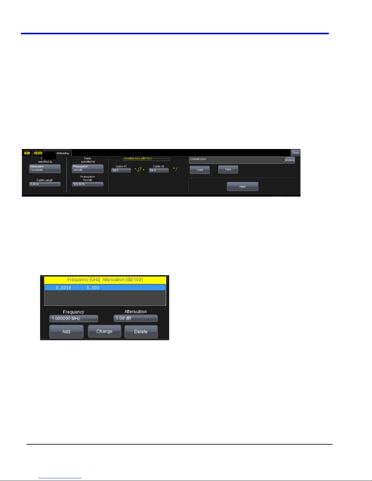
WavePro 7Zi
Cable De-Embedding
When making measurements on serial data signals, losses in the cables used in the test setup can reduce the
accuracy of your signal (for example, signal amplitude and risetime), as well as introduce Inter-Symbol
Interference. These cable effects can dramatically alter your serial data measurements and potentially create
mask test violations. The Cable De-Embedding option allows you to quickly specify the characteristics of the
cables (typically found on the cable's data sheet) in your test setup and analyze your signal with the effects of the
cables removed.
Setting Up Cable De-Embedding
Each of the four Channel menus has its own Cable De-Embedding dialog so that you can individually describe the
cable that is being used on each channel. You can specify your cable characteristics by entering either the
attenuation table for the cable or two attenuation constants of the loss model for the cable (provided by the cable
manufacturer). Then, you must specify the delay and physical length of the cable that you are using in your setup,
and you are ready to view your corrected signal. When you remove the effects of the cable, the compensated
signal is a more accurate representation of what was actually transmitted.
1. Touch Vertical Channelx Setup from the menu bar.
2. On the Channelx Setup dialog, touch to place a check mark in the Cable De-Embedding checkbox. A
Cable De-Embedding tab will be displayed.
3. Touch the Cable De-Embedding tab.
4. Touch inside the Cable Specified by data entry field and select Attenuation Constants if you want to
specify your cable characteristics by entering the two attenuation constants of the loss model for the cable
(provided by the cable manufacturer).
OR
Touch inside the Cable Specified by data entry field and select Attenuation Table
if you want to specify your cable characteristics by
entering the attenuation table for the cable (provided by the cable manufacturer). Enter an Attenuation
value and a Frequency and click Add to add them to the Attenuation Table. If you want to edit a row in the
table, highlight the row, change the Attenuation and Frequency and click Change. If you want to delete a
row, highlight the row and click Delete.
5. Touch inside the Delay Specified by data entry field to specify the delay. The cable delay can be either
Propagation Velocity, Nominal Delay, or a Dielectric Constant.
6. Touch inside the Cable Length data entry field and enter the physical length of the cable in inches.
7. Click Apply to initiate the cable de-embedding for the signal on this channel so that the effects of the cable
are removed.
Saving Cable Configurations
You should save cable configurations so that you can easily load them at another time. The current cable
configuration will not be preserved after exiting the application unless you save it.
23
WP700Zi-OM-E-RevA
Page 25

Operator's Manual
1. On the Cable De-Embedding dialog, touch inside the File Name [DefaultCable] data entry field and enter
a file name using the pop-up keyboard.
OR
Touch the Browse button and select a location and file name.
2. Touch the Save button.
Note: You can load previously saved cable configurations by touching the Browse button, locating the file and
then clicking Load.
Sequence Sampling Mode – Working with Segments
Using Sequence Mode, you can store up to 15,000 triggered events as "segments" into the oscilloscope's
memory. This is ideal when capturing many fast pulses in quick succession or when capturing few events
separated by long time periods. The instrument can capture in fine detail complicated sequences of events over
large time intervals, while ignoring the uninteresting periods between the events. You can also make time
measurements between events on selected segments using the full precision of the acquisition timebase.
Sequence mode offers a number of unique capabilities:
x You can acquire up to four channels simultaneously.
x You can minimize dead time between trigger events for consecutive segments.
x You can view time stamps for acquisitions.
x You can zoom segments or used them as input to math functions.
x You can combine sequence mode with an advanced trigger to isolate a rare event, capture all instances
over hours or days, and view/analyze each afterwards.
x You can use Sequence mode in remote operation to take full advantage of the instrument's high data-
transfer capability.
In Sequence mode, the complete waveform consists of a number of fixed-size segments acquired in single-shot
mode (see the instrument specifications for the limits). The oscilloscope uses the sequence timebase setting to
determine the capture duration of each segment: 10 x time/div. Along with this setting, the oscilloscope uses the
desired number of segments, maximum segment length, and total available memory to determine the actual
number of samples or segments, and time or points.
Figure 3-1. How the instrument captures segments
WP700Zi-OM-E-RevA
24
Page 26
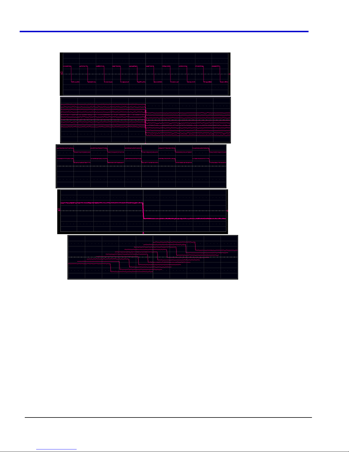
Sequence Display Modes
The instrument gives you a choice of five ways to display your segments:
x Adjacent
x Waterfall (cascaded)
x Mosaic (tiled)
WavePro 7Zi
x Overlay
x Perspective
Setting Up Sequence Mode
When setting up Sequence Mode, you define the number of fixed-size segments acquired in single-shot mode
(see the instrument specifications for the limits). The oscilloscope uses the sequence timebase setting to
determine the capture duration of each segment. Along with this setting, the oscilloscope uses the number of
segments, maximum segment length, and total available memory to determine the actual number of samples or
segments, and time or points.
25
WP700Zi-OM-E-RevA
Page 27
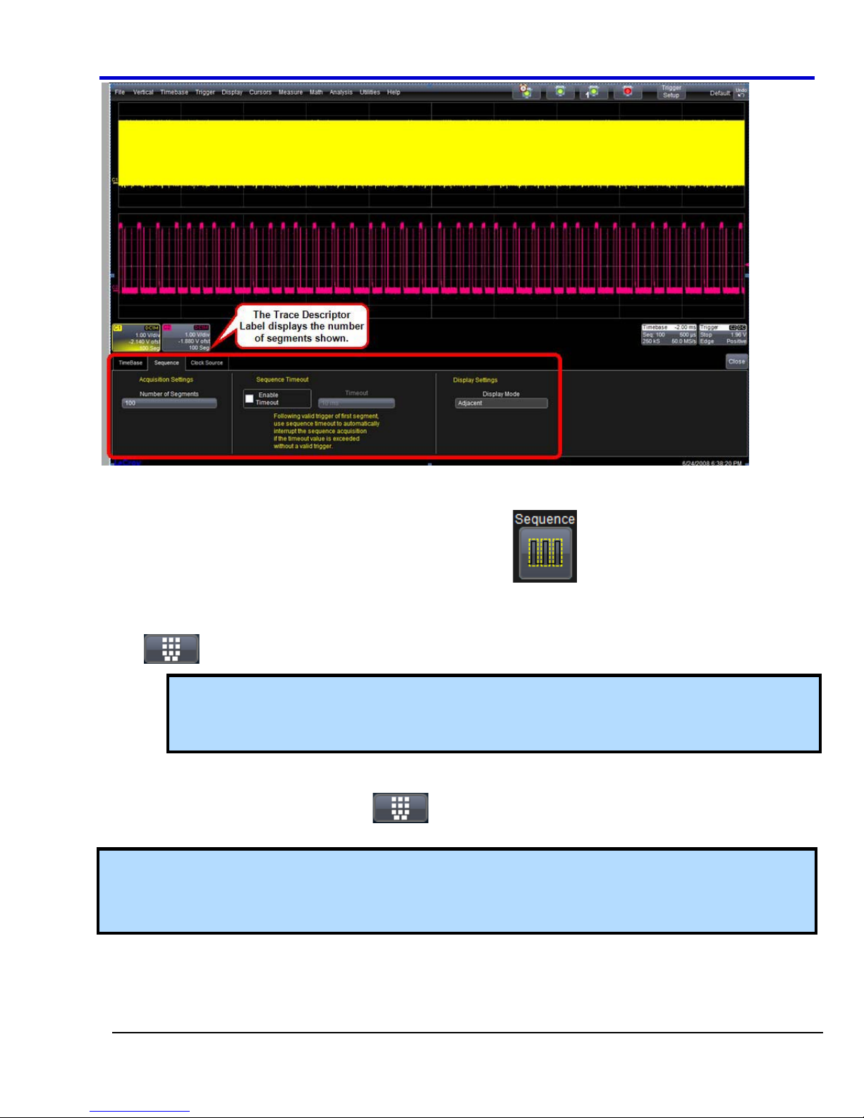
Operator's Manual
Figure 3-2. Setting up Sequence Mode (Adjacent)
1. Touch Timebase Horizontal Setup on the menu bar.
2. Under Sampling Mode, touch the Sequence mode button
3. Click the Sequence tab.
4. Under Acquisition Settings, touch inside the Num Segments data entry field and enter the number of
segments you want to display, using the slider bar at the bottom of the window. Click the keypad button
on the slider bar to enter a value using the pop-up numeric keypad.
Note: The number of segments you choose to display (80 maximum) can be less than the total
number of segments in the waveform. For example, in the pop-up images above, the number of
display segments is 10, but the total number of segments entered in the timebase dialog's Num
Segments field is 100.
5. Touch the Enable Timeout checkbox.
6. Touch inside the Timeout data entry field and enter a timeout value, using the slider bar at the bottom of
the window. Click the keypad button
keypad.
Note: Use the sequence mode timeout to automatically interrupt the sequence acquisition if the timeout value is
exceeded without a valid trigger. The timeout period accounts for instances when a Num Segments miscount
occurs for some reason and the scope waits indefinitely for an unforthcoming segment. During that time, no
oscilloscope functions are accessible. By means of a timeout value, however, the acquisition will be completed,
the waveform displayed, and control of the oscilloscope returned to the user after the timeout has elapsed.
on the slider bar to enter a value using the pop-up numeric
.
5. Under Display Settings, touch inside the Display mode field, and select a sequence mode display from
the pop-up menu.
6. Touch the S
WP700Zi-OM-E-RevA
INGLE trigger front panel button.
26
Page 28
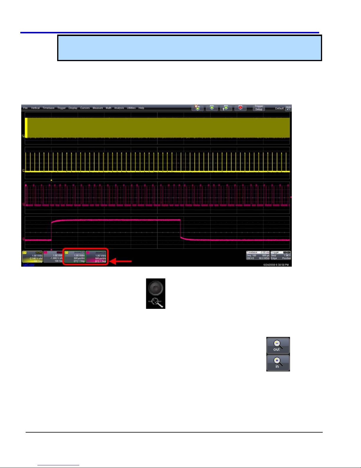
WavePro 7Zi
Note: Once a single acquisition has started, you can interrupt the acquisition at any time by
pressing the SINGLE front panel button a second time or by pressing the STOP front panel button. In
this case, the segments already acquired will be retained in memory.
Zooming Segments in Sequence Mode
You can zoom individual segments easily using the QUICKZOOM front panel button. When you zoom, the zoom
traces default to Segment 1. Channel descriptors indicate the total number of segments acquired. Zoom
descriptors indicate [Seg #] and #Segments in the Zoom. You can scroll through the segments using Z
panel position knob.
OOM front
Figure 3-3. Sample Zoom of Segments in Sequence Mode
1. Touch the front panel Quickzoom button .
2. Turn the Z
3. To vary the degree of zoom, touch the newly created Zx trace label. The setup dialog for the zoom (Z1 to
Z4) opens. It shows the current horizontal and vertical zoom factors.
4. If you want to increase or decrease your horizontal or vertical zoom in small increments, touch the Var.
checkbox to enable variable zooming. Now with each touch of the zoom control buttons , the
degree of magnification will change by a small increment.
OR
If you want to zoom in or out in large standard increments with each touch of the zoom control buttons,
leave the Var. checkbox unchecked.
OR
27
OOM front panel position knob to scroll through the segments.
WP700Zi-OM-E-RevA
Page 29
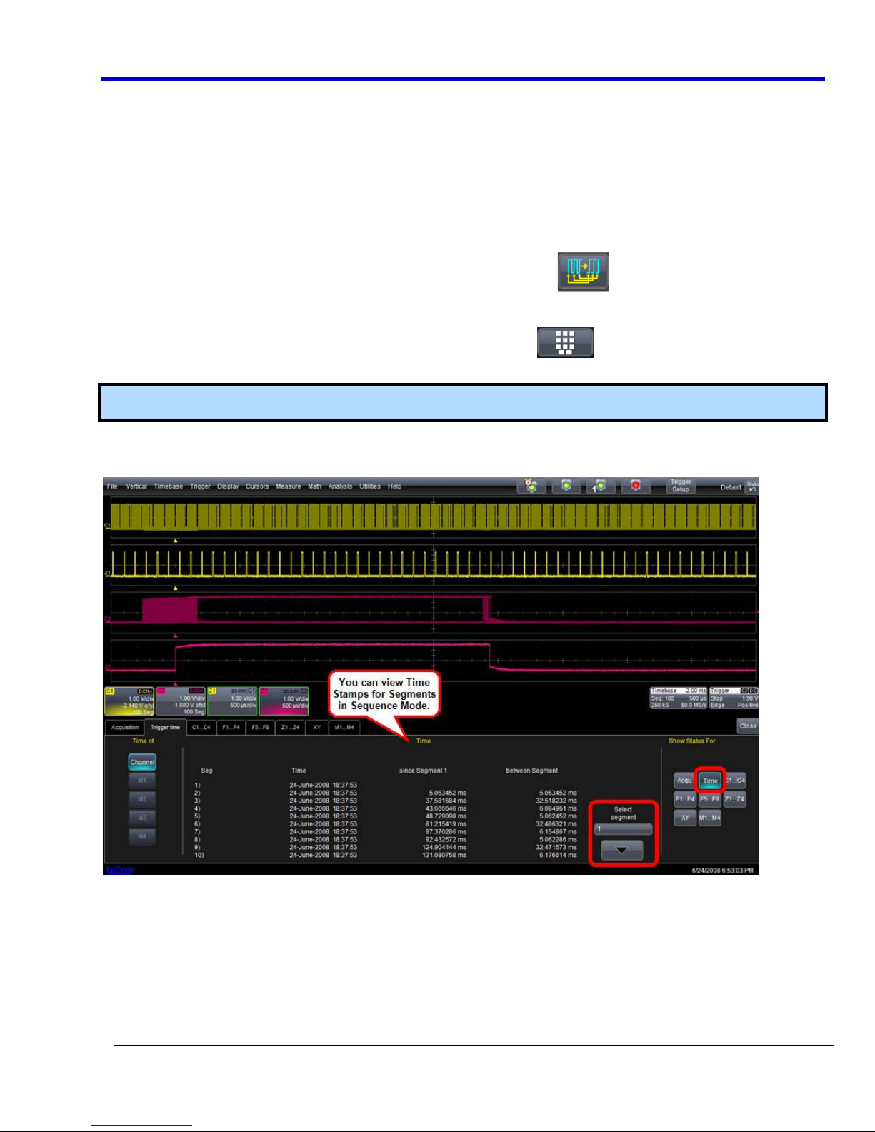
Operator's Manual
If you want to set exact horizontal or vertical zoom factors, touch inside the Horizontal Scale/div data
entry field and enter a time-per-div value, using the pop-up numeric keypad. Then touch inside the
Vertical Scale/div field and enter a voltage value.
Displaying an Individual Segment
1. Touch Math Math Setup on the menu bar.
2. Touch a function tab (F1 to Fx - The number of available math traces depends on the software options
loaded on the oscilloscope. Refer to the specifications for details).
3. Touch inside the Operator1 field and select the Segment button
4. In the dialog on the right, touch the Select tab.
5. Touch inside the First Selected data entry field and use the slider bat at the bottom of the window to select
the first segment you want to display. Click the keypad button
using the pop-up numeric keypad.
Note: In Persistence mode, the segments are automatically overlaid one on top of the other in the display. In nonPersistence mode, they appear separately on the grid.
from the pop-up menu.
on the slider bar to enter a value
Viewing Time Stamps
You can view time stamps for each segment.
1. Touch Timebase Acquisition Status on the menu bar.
OR
Touch Vertical Channel Status on the menu bar.
2. Touch the Trigger Time tab.
3. Under Show Status For, touch the Time button.
WP700Zi-OM-E-RevA
Figure 3-4. View Segment Time Stamps
28
Page 30
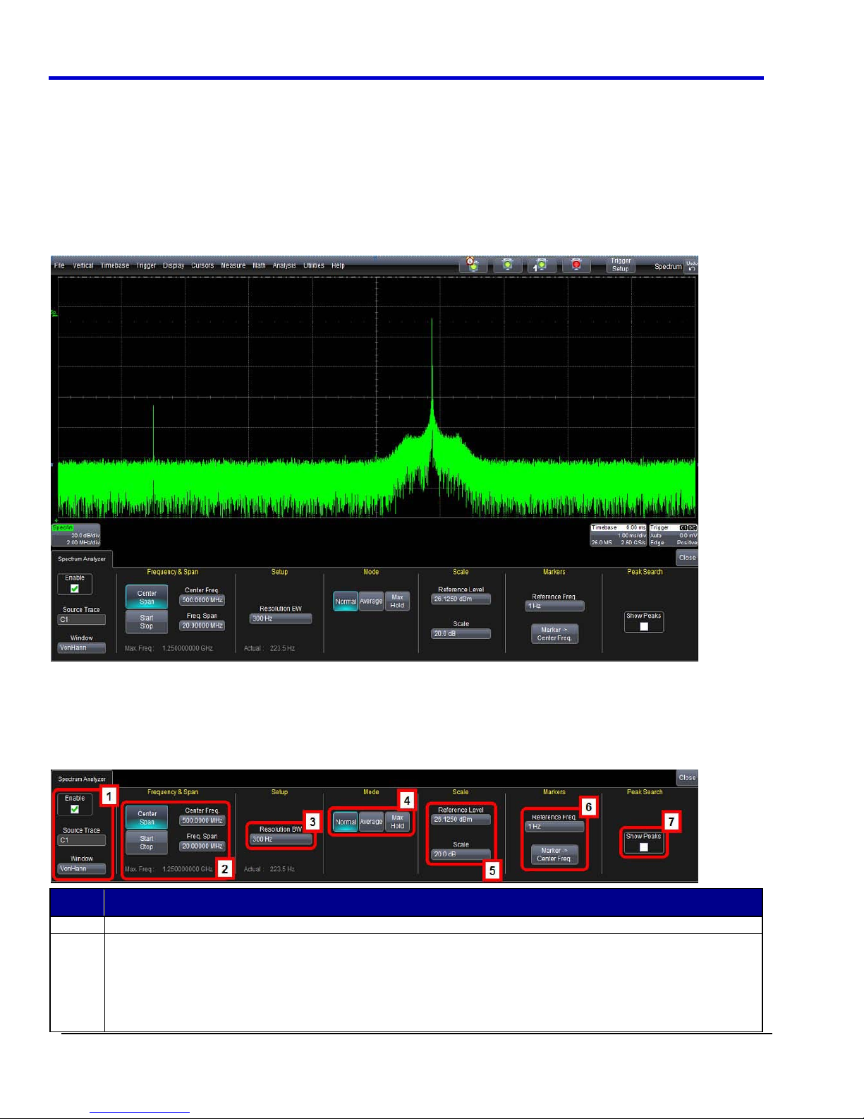
WavePro 7Zi
4. Touch inside the Select Segment field and enter a segment number, using the pop-up keypad or touch the
arrow buttons to scroll through segment times.
Spectrum Analyzer
The Spectrum Analyzer and Advance FFT option in the WavePro 700Zi series oscilloscopes will help you use the
Fast Fourier Transform (FFT) in your measurements. If you are familiar with RF spectrum analyzers, you can start
using the FFT with little or no concern about the details of setting up an FFT. The Spectrum Analyzer controls are
the same as you would find on an RF spectrum analyzer. You can set the span, center frequency and resolution
bandwidth and the oscilloscope automatically configures the acquisition and FFT controls to obtain the desired
spectrum view.
Figure 3-5. Sample dialog and display for the Spectrum Analyzer
Running the Spectrum Analyzer
You can run the Spectrum Analyzer by touching Analysis Spectrum Analyzer from the menu bar. When you
run the Spectrum Analyzer, you set up controls in the Spectrum Analyzer dialog from left to right, including a
Source, Center Frequency, Frequency Span, and Resolution Bandwidth.
NumberDescription
Enable the Spectrum Analyzer and choose the Source Trace.
1
Center Span is similar to adjusting the position of the FFT zoom trace. You enter the Center Frequency
and the Frequency Span. Frequency Span is similar to adjusting the zoom scale of the FFT. This does
not change the sample rate or memory. The Spectrum Analyzer reports the maximum frequency that can
2
be observed.
OR
29
WP700Zi-OM-E-RevA
Page 31

Operator's Manual
NumberDescription
Start Stop provides another way to adjust the position of the FFT zoom trace. You can specify the
Starting and Stopping Frequencies
Resolution Bandwidth is equivalent to changing the Timebase setting to increase or decrease memory
in FFT mode. Reducing the Resolution Bandwidth equals more memory. The Spectrum Analyzer reports
3
back adapted values for the resolution bandwidth if the value entered is not achievable.
There are three modes: Normal, Average, and Max Hold. In Averaging mode, you can enter the number
of spectra to be averaged. Averaging is effective in reducing the noise of the signal to see more of the
harmonic or carrier detail. Max (Peak) Hold mode is useful for swept frequency measurements where it
4
shows the history of peak values across the frequency axis. Max Hold shows the maximum level the
signal reaches. it is also useful for finding infrequent spurs.
Reference Level sets the amplitude of the top of the screen. Scale is the same as adjusting the Vertical
5
Gain knob in FFT mode.
Using Markers, you can set the reference frequency and display a marker for the center frequency.
6
Show Peaks lets you label and tabulate peaks. When Show Peaks is checked, the significant peaks are
marked with a frequency and gain stamp and a table listing the peaks, ordered by amplitude from highest
7
to lowest is displayed. This is very useful in identifying harmonics or peaks that may be hidden due to
poor resolution.
TriggerScan
TriggerScan is a debugging tool that helps you quickly find rare waveform glitches and anomalies. With
TriggerScan, you can build a list of trigger setups to look for rare events and automatically sequence through
each one. TriggerScan can use any type of trigger setup available including edge, width, and qualify as well as
Smart Triggers (such as, glitch and runt triggers). TriggerScan automates two key processes in triggering rare
events:
1. Trains the system by looking at normal acquired waveforms. During the training, the oscilloscope analyzes
the waveforms to determine what waveforms normally look like. Using this information, it generates a list of
smart trigger setups to trigger on abnormal situations.
2. Loads the smart trigger setups from the Trainer and cycles through these. As triggers occur, they are
overlaid on the screen. All acquisition settings are preserved and you can use all the functions of the
oscilloscope to find the root cause of these anomalies including, WaveScan, Histograms, and advanced
analysis.
WP700Zi-OM-E-RevA
30
Page 32

WavePro 7Zi
Training TriggerScan
The TriggerScan Trainer inspects a currently acquired waveform and automatically builds a list of common trigger
setups used to find rare events.
PLEASE NOTE THE FOLLOWING:
x You must acquire and display at least 3 cycles of a signal before running the Trainer.
x You should run the Trainer if you want to change the trigger types or if you change the channel or signal.
1. Touch Trigger Trigger Setup from the menu bar.
2. On the Trigger dialog, click the TriggerScan tab.
3. Touch inside the Source data entry field and select a channel as the source for the training.
4. Touch the Trainer button.
5. On the TriggerScan Trainer Setup window, choose the types of triggers the Trainer should use to train
the system and then touch the Start Training button. The training begins. When it is complete, a list of
smart trigger setups is displayed in the Trigger List.
31
WP700Zi-OM-E-RevA
Page 33

Operator's Manual
Starting TriggerScan
After you have run the Trainer, the Trigger List displays a list of smart trigger setups. You can add or remove
trigger setups. You can also update the selected smart trigger setup. Once you have made any changes to the
Trigger List, you are ready to start scanning.
1. Touch Trigger Trigger Setup from the menu bar.
2. On the Trigger dialog, click the TriggerScan tab.
3. If you want to add a new trigger setup, touch the Trigger tab and set the new trigger. Then, touch the Add
New button to add the new trigger to the Trigger List.
4. If you want to delete a trigger setup, highlight the setup in the Trigger List and touch the Delete Selected
button.
Note: If you want to delete all trigger setups in the Trigger List, touch the Delete All button.
5. If you want to replace the selected trigger setup with the current trigger setup, highlight the setup in the
Trigger List and touch the Update Selectedbutton.
6. Once you have made any changes to the Trigger List, touch Start Scan. The oscilloscope automatically
sequences through all the trigger setups.
PLEASE NOTE THE FOLLOWING:
x You can tune the dwell time that the scope will wait before loading the next trigger setup using the
Dwell Time data entry field.
x If you have Persistence display mode enabled, all trigger events are recorded on the display. Refer
to the Persistence Setup topic for instructions on enabling Persistence display mode.
x If you want TriggerScan to stop when the scope triggers next, check the Stop On Trigger
checkbox. You can use this to isolate specific trigger setups.
Saving TriggerScan Setups
You should save TriggerScan setups once you have made any modifications to the Trigger List. The current
Trigger List will not be preserved after exiting the application unless you save it.
1. On the TriggerScan dialog, touch inside the Setup File Name data entry field and enter a file name using
the pop-up keyboard.
OR
Touch the Browse button and select a location and file name.
2. Touch the Save Setup button.
Note: You can load previously saved TriggerScan setups by touching the Browse button, locating the file and
then clicking Load Setup.
WP700Zi-OM-E-RevA
32
Page 34

Front Panel
Numbered labels on this graphic correspond with descriptions in the table.
WavePro 7Zi
Number and Description Number and Description Number and Description
1. Power Button
2. Channel Row LED Indicator
3. Channel Inputs
4. Auxiliary Input and Output
5. Volume Control and Mute
Button
6. Ground Connector
7. Speaker
8. Fast Edge, Recovered Clock,
and Data Outputs
9. USB Ports
10. Detachable Front PanelRemote Control
11. Release Switch for Front
Panel-Remote Control
33
WP700Zi-OM-E-RevA
Page 35

Operator's Manual
Detaching and Attaching the Front Panel
Detach the front panel from the oscilloscope by sliding the detachment lever to the left and pulling at the right.
Attach the front panel by inserting the lower part first, sliding the detachment lever to the left, and then pushing
the top in place.
Front Panel as a Remote Control
While detached, the front panel can then act as a remote control. Just plug-and-play connect it to the oscilloscope
using a USB - A to USB - Mini B cable.
WP700Zi-OM-E-RevA
34
Page 36

WavePro 7Zi
Side Panel
The WavePro Zi side panel is located on the right side (facing the front of the instrument) as follows:
Numbered labels on this graphic correspond with descriptions in the table.
Number and Description Number and Description Number and Description
8. Speakers
9. Microphone
1. LBUS (LeCroy Bus)
2. Mouse
3. Keyboard
4. USB Ports
Note: Consult your system administrator when connecting to an internal LAN.
5. External VGA Monitor
6. Ethernet Port
7. Line In
10. PCI Expansion Slots for DVI
(for standard display
hardware), LSIB, and other
options (LeCroy External
Display WPZi-EXTDISP-15
option).
35
WP700Zi-OM-E-RevA
Page 37

Operator's Manual
Back Panel
Numbered labels on this graphic correspond with descriptions in the table.
Number and Description Number and Description Number and Description
1. External Clock Input
(Grounded EMI Shield
required when port is not in
use)
2. External Clock Output
WP700Zi-OM-E-RevA
3. Removable Hard Drive
4. DVD-CD + R Drive
5. Power Switch
6. DC Power Plug
36
Page 38

WavePro 7Zi
External Monitor
Setting up the External Monitor involves a connection and a few touch screen selections. It's a hot swap
connection, so there's no need to restart the instrument once you've connected.
1. Plug your external monitor (WPZi-EXTDISP15 option) display into the DVI and DC 12 connections on the
PCI slot (located on the side of the oscilloscope). Connect your USB plug (where applicable) to an
available port (also on the side of the instrument).
Note: To connect a standard VGA monitor, connect to the VGA Port.
2. Turn on the oscilloscope, let the instrument boot and then touch Display Display Setup... from the
menu bar.
3. Touch the Monitor tab and then the Enable External Monitor button.
4. Touch inside the Brightness field and adjust brightness as necessary.
37
WP700Zi-OM-E-RevA
Page 39

Operator's Manual
The following picture shows a WavePro 700Zi with the LeCroy external monitor attached (optional WPZiEXTDISP15).
WP700Zi-OM-E-RevA
38
Page 40

WavePro 7Zi
Dual Channel Acquisition
Combining Channels
Channels can be combined to increase sample rate, memory, or both in order to capture and view a signal in all
its detail. When you combine channels, uncombined channels like EXT BNC remain available for triggering, even
though they are not displayed.
In 2-channel operation, channels 2 and 3 are made active. Channels 1 or 2, and 3 or 4 can be used in Auto
operation for 20 GS/s. When channels are paired in the following combinations, the maximum sampling rate is
doubled and the record length is greatly increased:
Channel Combinations Receiving 40 GS/s
Channels 1 and 3
Channels 1 and 4
Channels 2 and 3
Channels 2 and 4
Note: These sample rates apply to all WavePro Zi oscilloscopes (except the 715Zi without the WPZi 1GHz 4x20
GS option).
In short, sampling can be maximized to 40GS/s using two channel combinations except for channels 1 and 2, or
channels 3 and 4 (which always yield 20 GS/s. Use best practice by choosing channel 1 or 2 for your first input,
and channel 3 or 4 for the second.
Refer to Acquisition Modes
Combining Channels Procedure
Set up channel combinations on the interface as follows:
1. Touch Timebase Horizontal Setup on the menu bar and the Horizontal Setup dialog is shown.
2. Under Active Channels, touch 4, 2 or Auto. The maximum sample rate is shown alongside each button.
in the specifications for maximum sample rates.
Hardware and Software Controls
The following Basic Control topics cover the general usage of the hardware buttons located on the oscilloscope's
front panel and the screen control interface elements of the software.
Front Panel Controls
Note: Some front panel controls correspond with screen layout controls in specific ways. For example, the Print
front panel general control button corresponds with the Hardcopy function at Utilities Utilities Setup
Hardcopy.
39
WP700Zi-OM-E-RevA
Page 41

Operator's Manual
The detachable WavePro Zi front panel.
WP700Zi-OM-E-RevA
40
Page 42
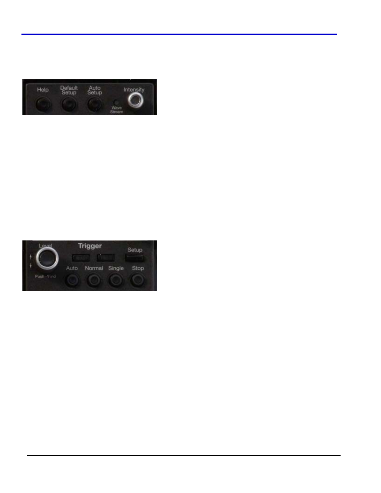
WavePro 7Zi
Front Panel Groupings
The front panel is divided into sections based on functions. The following sections explain them in a bit more
detail.
Miscellaneous Setup Controls
x Help - Press to open the LeCroy Online Assistant where you can click to open the oscilloscope online help
table of contents, index, or search for a topic using a keyword. If the second monitor is installed, the online
help opens on the second monitor.
x Default Setup - Press to reset the oscilloscope's settings to the default configuration. Corresponds with
screen menu selection: File Recall Setup Recall Default Setup. For a list of default settings, see
Save/Recall Saving and Recalling Scope Settings.
x Auto Setup - Press once and the Auto Setup flyout menu opens. Press the Auto Setup button on the
flyout menu to perform a full auto setup. Press a Channel Find Scale button on the flyout menu to perform
a quick auto setup for that channel only. Press the A
selection from the Auto Setup flyout menu (the default is to perform a full auto setup).
x WaveStream - Indicates when the acquisition mode is set to WaveStream.
x Intensity - Press to toggle between the most recently selected Acquisition/Sampling Mode and
WaveStream mode. When you turn the knob, if WaveStream is ON, the WaveStream display intensity
changes. When you turn the knob, if WaveStream is OFF, changes the Intensity setting. Corresponds with
the screen menu selection: Display Display Setup.
UTO SETUP front panel button twice to perform the last
Trigger Front Panel Controls
x Level - Press to toggle between 50% trigger level and the previous level setting. Turn to change the trigger
threshold level. This level is indicated on the Trigger label.
x Trigger - Indicates the trigger status as READY and TRIG'D. READY is lit when the trigger is armed.
TRIG'D is lit momentarily when a trigger occurs. A fast trigger rate will cause the light to stay lit
continuously.
x Setup - Press once to open the Trigger Setup dialog. Corresponds with screen menu selection: Trigger
Trigger Setup. Press the Trigger S
x Auto - Press to turn on Auto Trigger mode, which triggers the oscilloscope after a time-out, even if the
trigger conditions are not met.
x Normal - Press to turn on Normal Trigger mode, which triggers the oscilloscope each time a signal is
present that meets the conditions set for the type of trigger selected.
x Single - Press to turn on Single Trigger mode, which arms the oscilloscope to trigger once (single-shot
acquisition) when the input signal meets the trigger conditions set for the type of trigger selected. If the
scope is already armed, it will force a trigger.
x Stop - Press to prevent the scope from triggering on a signal. If you boot up the instrument with the trigger
in Stop mode, the message "no trace available" will be displayed. Press the Trigger A
button to display your trace.
ETUP front panel button again to close the Trigger Setup dialog.
UTO front panel
41
WP700Zi-OM-E-RevA
Page 43

Operator's Manual
x
x
x
Horizontal Front Panel Controls
Note: Horizontal front panel controls correspond with screen menu selection: Timebase Horizontal Setup.
x Delay - Press to toggle between a zero horizontal delay value and the previous horizontal delay value.
Turn to change the horizontal delay value.
x Time - Turn to set the time/division of the oscilloscope timebase (acquisition system). The time scale is
adjusted from the left edge of the display.
Vertical Front Panel Controls
Note: Vertical front panel controls correspond with screen menu selection: Vertical Channel Setup.
Channels - Press a Channel 1-4 front panel button to turn the channel on or off. When a Channel 1-4
front panel button is lit, the Vertical Offset and Volts/Div knobs are "active" for that channel only.
Offset - Press to toggle between a zero vertical offset value and the previous vertical offset value for the
selected channel. Turn to change the vertical offset value for the selected channel.
Gain - Press to toggle between fixed and variable gain adjustment. Turn to change the gain value.
Cursors Front Panel Controls
Note: Cursors front panel controls correspond with screen menu selection: Cursors Cursors Setup.
WP700Zi-OM-E-RevA
42
Page 44

WavePro 7Zi
x Absolute Cursor - Press to set the cursor position to the default 25% position, either horizontal or vertical
(depending on which cursor type your are using). Turn to adjust the position of the cursor (absolute cursor
or one of the two relative cursors).
x Cursor Type - Press one to turn cursors ON to the last cursor type selected. Each subsequent press
toggles through the cursor types (Off, Abs Horizontal, Rel Horizontal, Abs Vertical, or Rel Vertical).
x Relative Cursor - Press to set the relative cursor to the default 75% position, either horizontal or vertical
(depending on which cursor type you are using)Turn to adjust relative cursors. It does not work with
absolute cursor types.
WaveScan Front Panel Controls
Note: WaveScan front panel controls correspond with screen menu selection: Analysis WaveScan.
x Scroll - If WaveScan is On, turn to scroll through the table of WaveScan-filtered events. If WaveScan is
Off, turn to adjust the selected data entry field.
x On/Off - Press to toggle between WaveScan On and Off. This is the same as checking Enable in the
WaveScan dialog. When you turn WaveScan On, it turns on the WaveScan to the last enabled mode on
the last selected Channel with the last selected Filter method. It also turns on the Z1 trace with its source
as the WaveScan Channel and changes whatever display grid was selected to a dual grid with channels in
the top grid and the WaveScan Z1 trace in the bottom grid.
x Setup - Press once to open the WaveScan dialog. Corresponds with screen menu selection: Analysis
WaveScan. Press the WaveScan S
ETUP front panel button again to close the WaveScan dialog.
43
WP700Zi-OM-E-RevA
Page 45
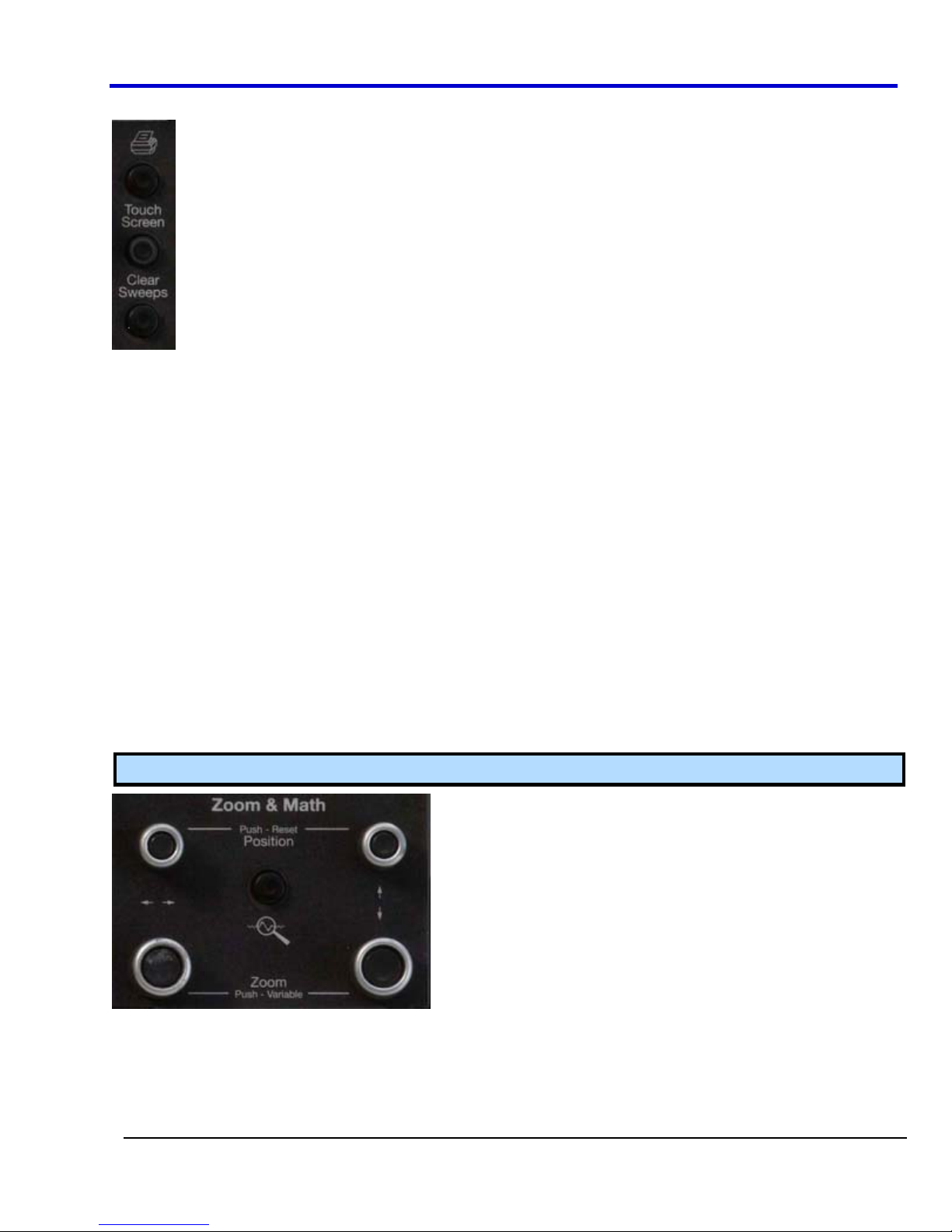
Operator's Manual
General Controls Front Panel Controls
x Print - Press once and the Print flyout menu opens.
Press the Print Now button on the flyout menu to print the current screen image using the Print settings on
the Utilities Utilities Setup Hardcopy dialog.
Press the Print Setup button on the flyout menu to open the Utilities Utilities Setup Hardcopy.
Press the Save Screen to file button on the flyout menu to save the screen image as a file to storage
media such as a USB drive or hard drive using the File settings on the Utilities Utilities Setup
Hardcopy dialog (incrementing the filename by one each time you touch Save Screen to File).
Press the Save Screen to Clipboard button on the flyout menu to save the current screen image to the
clipboard.
Press the Send Screen to Email button to send the current screen image using the email settings on the
Utilities Utilities Setup Hardcopy dialog.
Press the Create Notebook Entry button on the flyout menu to create a new lab notebook entry using the
Enter Notebook Info window.
Press the P
default is to print the screen image).
x Touch Screen - Press to toggle the touch screen on and off.
x Clear Sweeps - Press to clear data from multiple sweeps (acquisitions) including: persistence trace
displays, averaged traces, parameter statistics, and Histicons. During waveform readout, cancels
readout.This is the same as pressing Clear Sweeps on the Measure Measure Setup or Math Math
Setup dialogs.
RINT front panel button twice to perform the last selection from the Print flyout menu (the
Zoom and Math Front Panel Controls
Note: Zoom and Math front panel controls correspond with screen menu selection: Math Zoom Setup.
x Horizontal Position - Press to reset the horizontal zoom position to zero. Turn to change the horizontal
position of the selected math or zoom trace.
x Horizontal Ratio - Press to toggle between fixed and variable horizontal zoom ratio adjustment. Turn to
change the horizontal zoom ratio of the selected math trace.
WP700Zi-OM-E-RevA
44
Page 46

WavePro 7Zi
x
x
x
x Quick Zoom - Press to automatically display magnified views of up to four signal inputs on multiple grids.
With four input signals, the signals are displayed along with four zoom traces, each on its own grid.
Pressing this button also turns off all other traces.
x Vertical Position - Press to reset the vertical zoom position to zero. Turn to change the vertical position of
the selected math or zoom trace.
x Vertical Ratio - Press to toggle between fixed and variable vertical zoom ratio adjustment. Turn to change
the vertical zoom ratio of the selected math trace.
Screen Layout, Groupings, and Controls
The instrument's screen is divided into three main sections:
Menu Bar
Signal Display Grid
Dialog(s)
Note: Some front panel controls correspond with screen layout controls in specific ways. For example, the Print
front panel general control button corresponds with the Hardcopy function at Utilities Utilities Setup
Hardcopy.
Menu Bar
The top of the screen contains a menu bar of commonly used functions. Whenever you touch one of these
buttons and make a selection from its drop-down menu, the dialog area at the bottom of the screen displays the
corresponding dialog.
Specific Menu Bar functions are referenced using arrow-separated path descriptions. For example, the
Save Setup function is referenced as File Save Setup.
The Quick Access Toolbar
The Quick Access toolbar is located on the right side of the menu bar. You can use these toolbar buttons to
quickly access trigger functions.
x Auto - Press to turn on Auto Trigger mode, which triggers the oscilloscope after a time-out, even if the
trigger conditions are not met.
x Normal - Press to turn on Normal Trigger mode, which triggers the oscilloscope each time a signal is
present that meets the conditions set for the type of trigger selected.
x Single - Press to turn on Single Trigger mode for the selected channel, which arms the oscilloscope to
trigger once (single-shot acquisition) when the input signal meets the trigger conditions set for the type of
trigger selected. If the scope is already armed, it will force a trigger.
x Stop - Press to prevent the scope from triggering on a signal. If you boot up the instrument with the trigger
in Stop mode, the message "no trace available" will be displayed.
x Trigger Setup - Press to open the Trigger Setup dialog. Corresponds with screen menu selection:
Trigger Trigger Setup.
The Signal Display Grid
You can set up the signal display area by touching Display Display Setup from the menu bar. The Display
dialog offers a choice of grid combinations and can also set the grid intensity.
The following Display Grid features also provide assistance when using the oscilloscope:
x Descriptor Labels - For more information, go to the Trace Descriptors topic.
45
WP700Zi-OM-E-RevA
Page 47

Operator's Manual
x Pop-up Menu - You can click on a waveform to open a pop-up menu . From
this pop-up menu, you can perform the following functions:
x Open the Setup dialog for the trace
x Turn the trace descriptor label off
x Open the Math dialog for the trace
x Open the Measure dialog for the trace
x Annotate the selected trace
Dialog Area
The lower portion is where information is shown, selections are made, and data is input. Typically they are
organized into tabular displays, subtabs, or pop-up dialogs. The dialog area is controlled by touch screen buttons
and front panel buttons.
The following Dialog Area controls also provide assistance when entering data:
x Slider Bar - When you click in some data entry fields, a slider bar opens at the bottom of the screen.
You can use the slider bar on the left to make fine adjustments to the value. You can use the value
slider on the right to make coarse adjustments to the value. You can click on the value slider to set the
field to a specific value. Click the Default button on the slider bar to set the field to the default value.
Click the keypad button
x Flyout Menu - The Print and Auto Setup front panel buttons open flyout menus. For more information on
these menus, go to the Front Panel Groupings topic.
on the slider bar to set the value using the pop-up numeric keypad.
Universal ProBus/ProLink Interface
LeCroy's ProBus probe system provides a complete measurement solution from probe tip to oscilloscope display.
ProBus allows you to control gain and offset directly from your front panel. It is particularly useful for voltage,
differential, and current active probes. It uploads gain and offset correction factors from the ProBus EPROM's and
automatically compensates to achieve fully calibrated measurements.
This intelligent interconnection between your instrument and a wide range of accessories offers important
advantages over standard BNC and probe ring connections. ProBus ensures correct input coupling by autosensing the probe type, thereby eliminating the guesswork and errors that occur when attenuation or amplification
factors are set manually.
WP700Zi-OM-E-RevA
46
Page 48

WavePro 7Zi
The LeCroy WavePro 700Zi series oscilloscopes with bandwidths of 4 to 6 GHz include universal ProBus/ProLink
probe interfaces. As shown in the following figure, each channel has a high bandwidth ProLink connector and a
50 /1 M ProBus connector.
Figure 3-6. A WavePro760 Zi showing the four sets of ProBus/ProLink probe interfaces. This oscilloscope
is compatible with all LeCroy probes.
This unique interface provides the user the greatest flexibility in probe selection in any oscilloscope. The ProLink
inputs provide a high integrity, high bandwidth interchangeable interface to SMA cables, LeCroy ProLink probes,
and accessories. ProLink is used for higher bandwidth probes.
The ProBus interface offers both 50 /1 M input impedance and provides probe power and control for a wide
range of probes such as high impedance passive probes, high impedance active probes, current probes, high
voltage probes, differential probes. ProBus also includes sense rings for detecting passive probes. All scopes with
bandwidths over 4 GHz, except the WavePro 740Zi and760Zi, use 50 inputs and provide 1 M impedance by
means of external adapters.
The following figure shows a typical channel setup. The input selection is on the left hand side of the dialog box.
In this case the A input, the ProLink interface is selected. Each input selection has its own independent settings
for Probe attenuation, bandwidth and coupling.
Figure 3-7. The channel screen layout showing Input A's ProLink interface controls setup
Note: Input A (Upper) and B (Lower) refer to the two rows of input channels specifically available on WavePro
740 and 760Zi. WavePro 715, 725, and 735Zi all have only one row of input channels on the front panel, and
one corresponding selected input on the screen layout.
47
WP700Zi-OM-E-RevA
Page 49

Operator's Manual
The setup for the ProBus interface is shown in the following figure. This interface also allows the selection of input
impedance, 50 /1 M.
Figure 3-8. The channel screen layout showing Input B's ProBus interface controls setup
Another universal probe interface advantage is the ability to switch between two probe setups. This function is
remotely programmable allowing the interface to operate like a switch.
The characteristics of the universal ProBus/ProLink Interface are shown in the following table. Each of the
interfaces provide power to the probe. An I
recognition and interaction. This adds to the flexibility of the system as the scope can sense and control each
probe.
2
C interface allows communication with the probe which permits probe
Probe Interface
50 3.5 GHz 4-6 GHz
1 M 500 MHz NA
Table 3-1.Probe interface characteristics
The WavePro 740Zi and 760 Zi oscilloscopes offer the universal ProBus/ProLink probe interface which allows
dual inputs in the DC to 3.5 GHz range and a dedicated high bandwidth interface in the range of 4 through 6 GHz.
The ability to select four out of eight inputs provides unheard of connection flexibility and eliminates the need for
costly, easy to lose adapters.
ProBus
(Bandwidth)
ProLink
(Bandwidth)
WP700Zi-OM-E-RevA
48
Page 50
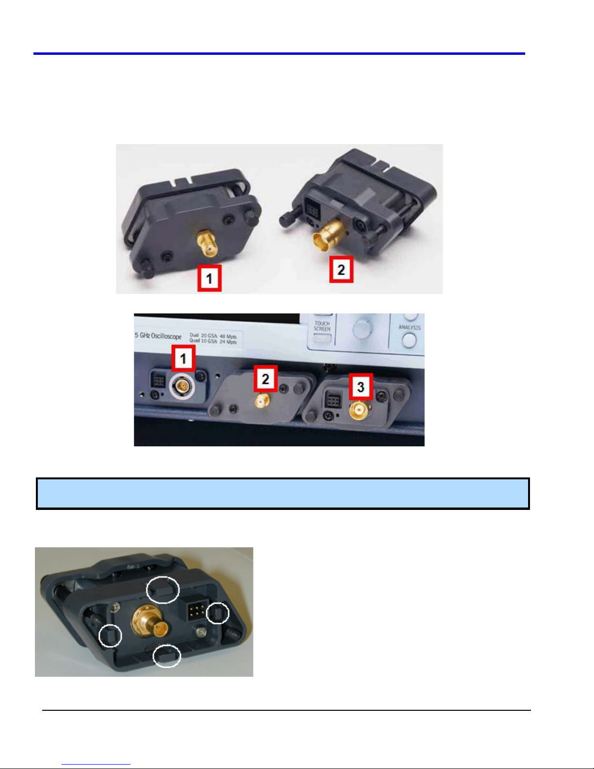
WavePro 7Zi
ProLink Interface
For some instruments, LeCroy's ProLink Adapters (LPA) give you the ability to connect your signal in one of three
ways:
x BMA connector (only on 4 and 6 GHz models)
x SMA using the BMA-to-SMA adapter (4 are sent standard on 4 and 6 GHz models)
x BNC using BMA-to-BNC adapter (optional)
Figure 3-9. BMA-to-SMA Adapter (1) and BMA-to-BNC Adapter (2)
Figure 3-10. BMA Female Connector (1), ProLink BMA-to-SMA Adapter (Installed, 2), and ProLink BMA-to-
BNC Adapter (Installed, 3)
Note: When connecting an active probe to the instrument, be sure to use a ProLink BMA-to-BNC adapter (item
3 in the figure). Do not plug the probe directly into the front panel connector (item 1) without an adapter.
Connecting the Adapters
The mating end of the ProLink adapter has four fastening clips as follows:
49
WP700Zi-OM-E-RevA
Page 51

Operator's Manual
When installing an adapter on the instrument's connector panel, align the male 6-pin connector with the female
connector and push the adapter straight in. There will be some resistance and you'll hear clicks as the four clips
slide into place. Then tighten the captive screws.
When removing an adapter, loosen the two captive screws. Push down on the adapter to unseat the clips. This
will require some force and will be initially noisy, but no damage will result to the connector, the floating female
BMA connector, or the pins, which can be 15 degrees off axis when being mated or unmated.
Auxiliary Output Signals
In addition to a calibration signal, the following signals can be output through the AUX OUTPUT connector:
Square Wave
Trigger Out - can be used to trigger another scope
DC level - a reference level (not available on all instruments)
Trigger Enabled - can be used as a gating function to trigger another instrument when the scope is
ready
Pass/Fail - allows you to set a pulse duration from 1 ms to 500 ms; generates a pulse when pass/fail
testing is active and conditions are met.
Aux Output Off - turns off the auxiliary output signal
Auxiliary Output Setup
1. Touch Utilities Utilities Setup... from the menu bar.
2. Touch the Aux Output tab.
3. If you want a 1 kHz, 1 V square wave, touch the corresponding button.
4. If you want a specialized output, touch one of the buttons under Use Auxiliary Output For.
5. Touch inside the Amplitude data entry field and enter a value, using the pop-up numeric keypad. If you
want a TTL level signal, touch the TTL Level checkbox. The Amplitude field will accordingly become
unavailable.
6. If you selected Square Wave, touch inside the Frequency data entry field and enter a value, using the
pop-up keypad. You can set a value from 5.0 Hz to 5 MHz.
7. If you selected Pass/Fail, touch inside the Pulse Duration field and enter a value from 1 ms to 500 ms,
using the pop-up numeric keypad.
WP700Zi-OM-E-RevA
50
Page 52

WavePro 7Zi
Pass/Fail Testing
Comparing Parameters
Each Pass/Fail input (Qx) can compare a different parameter result to a user-defined limit (or statistical range)
under a different condition.
The conditions are represented by these comparison operators:
At the touch of a button, test results can also be compared to these standard statistical limits:
In Dual Parameter Compare mode, your X-Stream oscilloscope can take parameter results measured on two
different waveforms and compare them to each other. If desired, set your test to be true if Any or All waveforms
fit the criteria set by the comparison condition. Setups are conveniently shown in the Summary box of the Qx
dialog as follows:
Mask Tests
Mask testing can be done using an existing mask, or by using a mask created from your actual waveform, with
vertical and horizontal tolerances that you define. Existing masks can be loaded from a floppy disk or from a
network.
You can set your mask test to be True for waveforms All In, All Out, Any In, or Any Out. For example, if you select
All In, the test will be False if even a single waveform falls outside the mask.
Masks that you create from your waveform can be confined to just a portion of the trace by use of a measure
r more information on how this feature works.
gate. Refer to the Measure Gate topi
c fo
51
WP700Zi-OM-E-RevA
Page 53

Operator's Manual
Actions
By touching the Stop Test checkbox
in the Actions dialog, you can set
up the test to end after a predetermined number of sweeps that you decide.
You can also decide the actions to occur upon your waveforms' passing or failing, by selecting one or all of the
following:
x stop
x audible alarm
x print image of display
x emit pulse (if available)
x save waveform
The selection Pulse causes a pulse to be output through the Aux Out connector at the front of the
oscilloscope. This pulse can be used to trigger another oscilloscope. You can set the amplitude and width of the
pulse as described in Auxiliary Output Signals.
Depending on your scope model, you can configure up to 8 pass/fail conditions. The boolean conditions to
determine if your waveform passes are as follows:
All True All False
Any True Any False
All Q1 to Q4 Or All Q5 to Q8 Any Q1 to Q4 And Any Q5 to Q8
Pass/Fail Testing Setup
Initial Setup
1. Touch Analysis Pass/Fail Setup... from the menu bar.
2. Touch the Actions tab.
3. Touch the Enable Actions checkbox. This causes selected actions to occur on your waveform's passing
or failing a test.
4. Touch the Summary View checkbox to enable a line of text
showing a concise status of the
last waveform and keeping a running count of how many sweeps have passed.
5. Touch inside the Pass If field, and select a boolean condition from the choices shown.
6. If you want to set up the test to end after a finite number of sweeps, touch the Stop Test checkbox. Then
touch inside the After data entry field and enter a value, using the pop-up numeric keypad.
7. Use either the Pass
when your waveform passes or fails the test.
8. The Then section of the dialog provides stop test, sound alarm, print result, emit pulse, or save (the
waveform) actions. If you want to have the results printed and your scope is not equipped with a printer, be
sure that the it is connected to a local or network printer. Refer to the Printing topics
9. If you want to save your waveform automatically, touch the Save Setup checkbox. This will take you out of
the current dialog and will open the Save Waveform dialog. Refer to the Save Recall Saving and
Recalling Waveforms topic for more information.
10. Test Pass/Fail conditions by touching the Force Actions Once button. Press the Clear All button to
quickly uncheck all checkboxes and make new selections.
or Fail button on the If section of the dialog to set actions taking place
for more
information.
WP700Zi-OM-E-RevA
52
Page 54

WavePro 7Zi
Comparing a Single Parameter
1. Touch Analysis Pass/Fail Setup... from the menu bar.
2. Touch one of the Qx tabs and a setup dialog for the position is shown.
3. Touch inside the Source1 field and select a source from the pop-up menu.
4. Touch inside the Condition field in the main dialog and select ParamCompare
5. Touch inside the Compare Values field and select All or Any from the pop-up menu . By selecting
All, the test will be true only if every waveform falls within the limit that you will set. By selecting Any, the
test will be true if just one waveform falls within the limit.
6. Touch inside the Condition field on the ParamCompare part of the dialog and select a math operator from
the pop-up menu .
7. Touch inside the Limit field and enter a value using the pop-up numeric keypad. The value entered
acquires the dimensions corresponding to the parameters being tested. For example, if you are testing a
time parameter, the unit is seconds.
.
If you chose either WithinDeltaPct
have the choice of setting the limit by means of the statistical buttons at the bottom of the ParamCompare
dialog:
Comparing Dual Parameters
1. Touch Analysis Pass/Fail Setup... from the menu bar.
2. Touch one of the Qx tabs and a setup dialog for the position is shown.
3. Touch inside the Condition field in the main dialog and select DualParamCompare
4. Touch inside the Source1 and Source2 fields and select a source from the pop-up menu.
5. Touch inside the ParamCompare mini-dialog field and select a source from the pop-up menu.
53
or WithinDeltaAbs from the Condition menu, you also
.
WP700Zi-OM-E-RevA
Page 55

Operator's Manual
6. Touch inside the Compare Values field and select All or Any from the pop-up menu . By selecting
All, the test will be true only if every waveform falls within the limit that you will set. By selecting Any, the
test will be true if just one waveform falls within the limit.
7. Touch inside the Condition field in the ParamCompare mini-dialog and select a math operator from the
pop-up menu .
8. Touch inside the Limit field and enter a value, using the pop-up numeric keypad. This value takes the
dimension of the parameter that you are testing. For example, if you are testing a time parameter, the unit
is seconds.
9. If you chose either WithinDeltaPct
inside the Delta field and enter a value.
or WithinDeltaAbs from the Condition menu, touch
Mask Testing
1. Touch Analysis Pass/Fail Setup... from the menu bar.
2. Touch one of the Qx tabs and a setup dialog for the position is shown.
3. Touch inside the Source1 field and select a source from the pop-up menu.
4. Touch inside the Condition field in the main dialog and select Mask Test
5. From the Test portion of the dialog, make a selection in the Test is True when group of buttons
. This selection means, for example, that if you select All In the test is False when a
single waveform falls outside the mask.
6. From the Show Markers section of the dialog, choose whether or not to have mask violations displayed.
7. If you are loading a pre-existing mask, touch the Load Mask tab, and then the File button. You can then
enter the file name or browse to its location.
8. If you want to make a mask from your waveform, touch the Make Mask tab.
9. Touch inside the Ver Delta and Hor Delta fields and enter boundary values, using the pop-up numeric
keypad.
10. Touch the Browse button to create a file name and location for the mask if you want to save it.
11. Touch the Gate tab, then enter values in the Start and Stop fields to constrain the mask to a portion of the
waveform. Or, you can simply touch and drag the Gate posts, which initially are placed at the extreme left
and right ends of the grid.
.
WP700Zi-OM-E-RevA
54
Page 56

WavePro 7Zi
Introduction to WaveScan
WaveScan enables you to search for unusual events in a single capture, or to scan for an event in many
acquisitions over a long period of time. You can select from more than 20 search modes (frequency, rise time,
runt, duty cycle, etc.), apply a search condition (slope, level, threshold, hysteresis), and begin scanning in a postacquisition environment. Since the scanning modes are not simply copies of the hardware triggers, but "software
triggers," the capability is much greater.
For instance, there is no “frequency” trigger in any oscilloscope, yet WaveScan allows frequency to be quickly
scanned for. You can accumulate a data set of unusual events that are separated by hours or days, enabling
faster debugging. The events are time stamped and indexed in a table from which you can select them for viewing
individually.
You can also set actions to occur automatically when unusual events are found: stop the acquisition, emit an
audible beep, output a pulse
, print the screen, save the waveform, or create a LabNotebook™ entry.
Signal Views
WaveScan provides distinct views of your signal:
x Source
x Scan Overlay
a separate grid. You can apply monochromatic persistence in this view.
x Scan Histogram
your search criteria.
x Zoom
processing ; to store it, or to apply a descriptive label to the feature.
Note: The number of grids displayed varies from one to three grids depending on which views are enabled.
WaveScan handles this function automatically, and there is no option to move traces from one grid to another,
as would be the case under normal (non-WaveScan) operation.
view highlights all occurrences of edges that meet your criteria.
(not available in WaveSurfer Xs scopes) places all captured edges one on top of the other in
(not available in WaveSurfer Xs scopes) provides a statistical view of edges that meet
view allows you to expand a waveform feature vertically and horizontally; to apply further
Search Modes
Search modes are used to locate anomalies during acquisition.
55
WP700Zi-OM-E-RevA
Page 57

Operator's Manual
x Edge - for detecting the occurrence of edges; selectable slope and level
x Non-monotonic
x Runt
x Measurement
- for detecting pulses that fail to cross a threshold; selectable polarity and thresholds
- for detecting threshold re-crosses; selectable slope, hysteresis, and level
- for filtering and performing parameter measurements
Parameter Measurements
Besides parameter measurements made during acquisition, post-acquisition measurements can also be made.
The number of parameters available depends on the options loaded on your instrument. Measurements are made
only on the events defined by your filter (search criteria). A Filter Wizard
criteria such as ±1, 3, or 5 sigma.
is provided to quickly establish statistical
Sampling Mode
Whenever WaveScan is enabled, the instrument reverts to Real-time sampling mode.
Source View
The top trace on the screen is the source (channel, math, memory) trace. This trace shows all captured edges
and highlights those that fit your search criteria. For example, in this figure we are searching for slow rising edges
that fall outside a time window:
In this acquisition, WaveScan has located eleven edges that fit the search criteria (filter) of greater than 1.2 ns
with a delta of 50 ps. Each of the found edges is highlighted with a red rectangle, and indexed to a table entry at
left. Rise time values are also included in the table.
Level Markers
Markers are provided on the source trace to show measurement criteria such as level and thresholds. In the
example above, the level markers indicate 10% and 90% for the standard Rise Time parameter measurement.
Level markers are displayed only while the scope is in WaveScan mode. Once the WaveScan Enable checkbox
is unchecked, the level markers disappear.
WP700Zi-OM-E-RevA
56
Page 58

WavePro 7Zi
Scan Overlay
This display mode shows all edges in an acquisition overlaid one on top of the other. By default, monochromatic
persistence is turned on for the scan overlays, but you have the option to disable it. Saturation and persistence
time controls are also available.
Note: The Saturation and Persistence Time set in the ScanOverlay dialog control the settings in the Display
Persistence setup dialog, and vice versa.
In the following acquisition, we have scanned for rise times greater than 1.4 ns. WaveScan has located six edges
that meet this criteria, one of which is greater than 2 ns. This slowest edge, which appears in the persistence
display, has been selected for zooming from the table. Note that it is also highlighted in the source view (top grid).
The horizontal scale of the overlaid traces can be expanded independently of the zoom trace. However, the
previous example shows them in the same scale as the zoom trace (5 ns/div).
57
WP700Zi-OM-E-RevA
Page 59
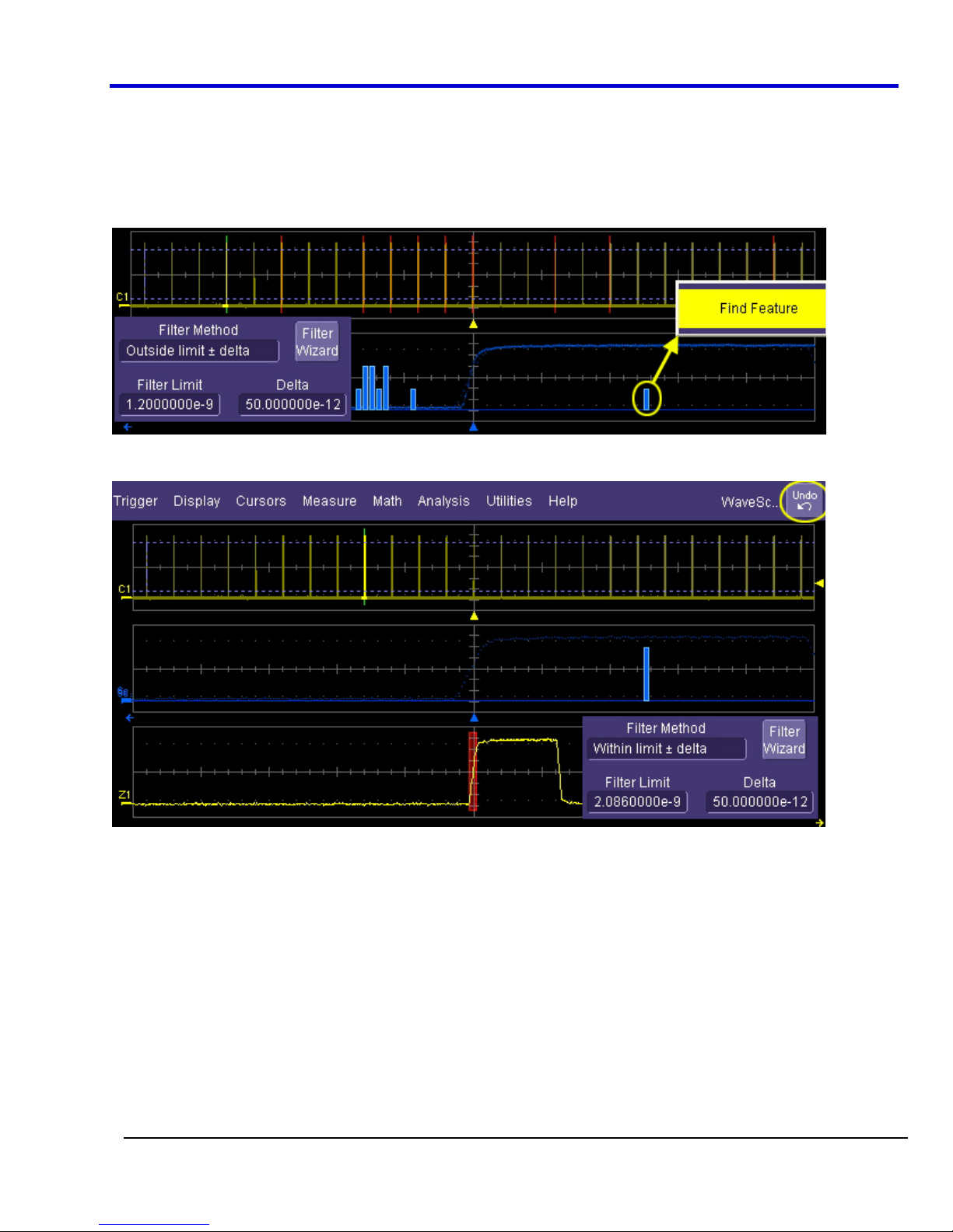
Operator's Manual
Scan Histogram
By enabling ScanHistogram, a histogram corresponding to your search criteria is superimposed on the overlay
trace. In the following example, the Rise 10-90% parameter measurement has been applied, but only edges
slower than 1.2 ns with a delta of 50 ps are accumulated in the histogram.
Another feature of WaveScan is that you can select a single bin of the histogram for analysis by touching or
clicking it. A confirmation pop-up button then appears:
After Find Feature is confirmed, only the single bin of the histogram remains and information about the contents
of the bin is displayed in the Filter Method area:
You can recall the original filter conditions by touching the Undo button at the top-right corner of the screen.
WP700Zi-OM-E-RevA
58
Page 60
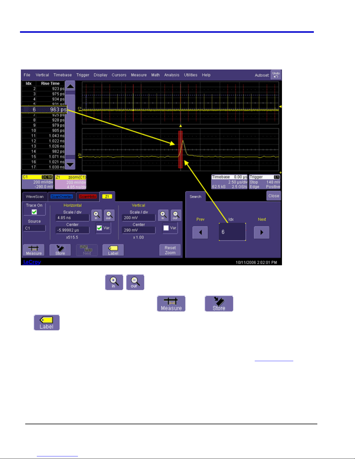
WavePro 7Zi
Zoom View
An individual edge can be zoomed by selecting it from the table of found events at the left of the screen. You can
also scroll through the table using the Prev/Next scroll buttons in the Search dialog, or select an event by
touching inside the Idx field and entering an index number, using the pop-up keypad.
Front panel
use the on-screen In/Outbuttons .
In Zoom View, you can also apply further processing , store , or apply a descriptive
label to the zoom trace.
ZOOM controls can be used to vary the magnification and position of the zoomed trace. Or, you can
Edge Mode
This search mode locates all edges in an acquisition and presents them time-stamped in a table. You can select
positive, negative, or both edges. When the acquisition is stopped, scan filters contained in Measurements
can be applied to the edges to find specific characteristics.
A level marker, corresponding to 50% in this case, is displayed in the source trace at top.
59
WP700Zi-OM-E-RevA
mode
Page 61
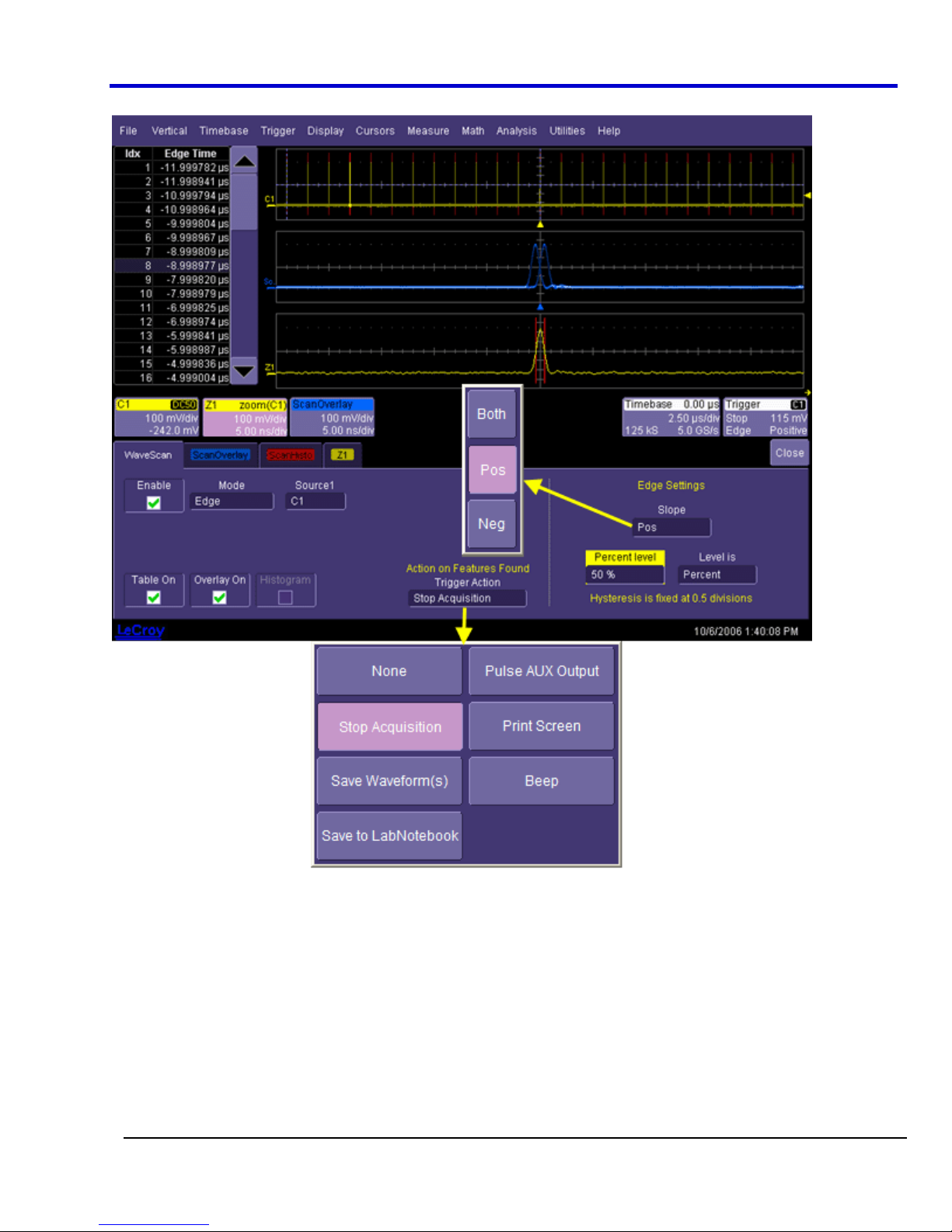
As with other search modes, a trigger action can be set for Edge mode also.
Operator's Manual
WP700Zi-OM-E-RevA
60
Page 62
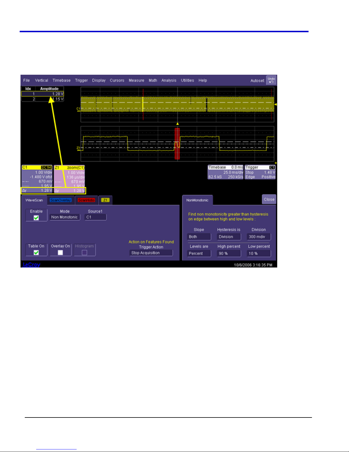
WavePro 7Zi
Non-monotonic Mode
The Non-monotonic search mode looks for edges that cross a threshold more than once between high and low
levels. All events that meet the criteria of slope, hysteresis, and level are presented in a table and highlighted in
the source trace. The value displayed in the table is the difference of the max. and min. of the non-monotonicity.
This can be confirmed with cursors:
The hysteresis value is used to eliminate noise. A non-monotonicity is detected only when its amplitude is greater
than the hysteresis. Therefore, when setting a hysteresis level, set a value that is greater than the amplitude of
the noise.
61
WP700Zi-OM-E-RevA
Page 63

Operator's Manual
Runt Mode
This search mode looks for pulses that fail to transit a given region. You can search for positive-going or negativegoing runts, or both. An adjustable hysteresis band is provided to eliminate noise.
In the case of negative-going runt pulses, the value displayed in the table is the difference (delta) of the high level
of the signal and the runt amplitude, i.e., where the runt bottoms out. This can be confirmed by placing cursors on
the runt pulse and reading the delta Y value in the trace labels:
In the case of positive-going runt pulses, the value displayed in the table is the absolute value of the amplitude of
the runt pulse:
WP700Zi-OM-E-RevA
62
Page 64

WavePro 7Zi
Measurement Mode
This search and scan mode lets you apply filters to your acquisitions to highlight only the features of interest.
Post-acquisition, you can apply other filters to the acquisition, or make different parameter measurements on it.
For example, in this acquisition a Rise time (10-90%) parameter measurement is applied to fast edges during
acquisition. We are interested only in edges with a rise time slower than 1 ns. Therefore, the Greater Than filter
method is selected, with a value of 1 ns; four edges pass during acquisition:
63
WP700Zi-OM-E-RevA
Page 65

Operator's Manual
Scan Filters
But, now we want to look at fall times greater than 3 ns; fifteen falling edges from the same acquisition pass this
new filter:
You can also decide how anomalous the features located should be by using the Filter Wizard
average value as the limit, to search for rarest events, or to apply statistical criteria.
to select the
Filter Wizard
You can decide how anomalous the features searched or scanned for should be by using the average value as
the limit, by searching for rarest events, or by applying statistical criteria: ±1, 3, or 5 sigma.
WP700Zi-OM-E-RevA
64
Page 66

WavePro 7Zi
In the following example, there were several slow edges in a repetitive waveform. For each filtering method
selectable from the wizard, the rise time used as the filter limit and delta are calculated automatically.
Filter Methods
While the Filter Wizard provides a quick way to apply filtering criteria automatically, the Filter Method menu and
related fields let you manually set up filtering criteria. And unlike the Filter Wizard selections, which are restricted
to absolute deltas, the Filter Method menu also offers deltas as percentages:
65
WP700Zi-OM-E-RevA
Page 67
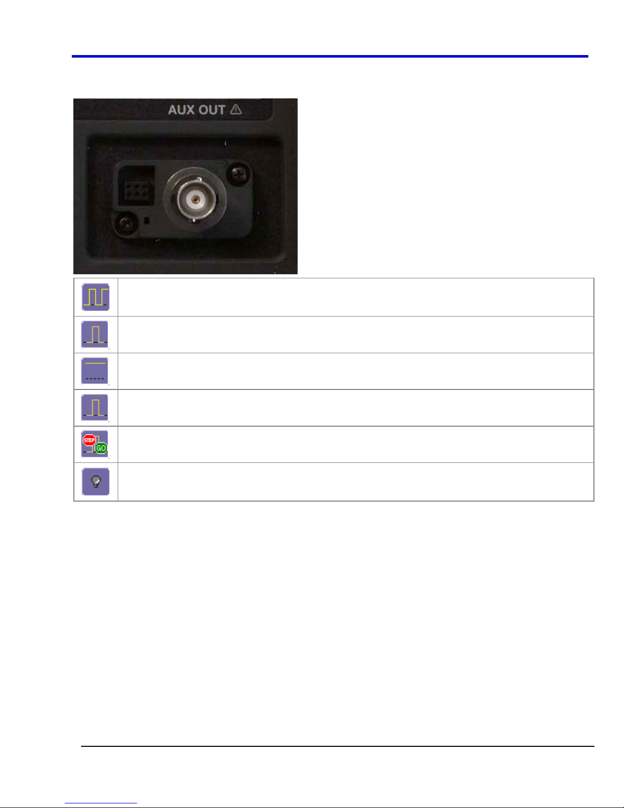
Operator's Manual
Auxiliary Output Signals
In addition to a calibration signal, the following signals can be output through the AUX OUTPUT connector:
Square Wave
Trigger Out - can be used to trigger another scope
DC level - a reference level (not available on all instruments)
Trigger Enabled - can be used as a gating function to trigger another instrument when the scope is
ready
Pass/Fail - allows you to set a pulse duration from 1 ms to 500 ms; generates a pulse when pass/fail
testing is active and conditions are met.
Aux Output Off - turns off the auxiliary output signal
Auxiliary Output Setup
1. Touch Utilities Utilities Setup... from the menu bar.
2. Touch the Aux Output tab.
3. If you want a 1 kHz, 1 V square wave, touch the corresponding button.
4. If you want a specialized output, touch one of the buttons under Use Auxiliary Output For.
5. Touch inside the Amplitude data entry field and enter a value, using the pop-up numeric keypad. If you
want a TTL level signal, touch the TTL Level checkbox. The Amplitude field will accordingly become
unavailable.
6. If you selected Square Wave, touch inside the Frequency data entry field and enter a value, using the
pop-up keypad. You can set a value from 5.0 Hz to 5 MHz.
7. If you selected Pass/Fail, touch inside the Pulse Duration field and enter a value from 1 ms to 500 ms,
using the pop-up numeric keypad.
WP700Zi-OM-E-RevA
66
Page 68

WavePro 7Zi
Customization Overview
The instrument provides powerful capability to add your own parameters, functions, display algorithms, or other
routines to the scope user interface without having to leave the instrument application environment. You can
customize the instrument to your needs by using the power of programs such as Excel™, Mathcad™, and
MATLAB™, or by scripting in VBS. Whichever method you use, the results appear on the instrument's display
together with the signals that you started with. This ability offers tremendous advantages in solving unique
problems for a large range of applications, with comparatively little effort from you.
Caution
Accessing the scope's automation interface from within an XDEV custom processor (VBScript, MATLAB, Excel,
etc.) is NOT recommended.
Cases where the scope's behavior cannot be guaranteed, or worse, cases which can cause the scope's
software to crash include the following:
1. Changing "Upstream" Controls
Upstream controls are considered to be any control that, if changed, could provoke an infinite loop. An example
would be a VBScript processor, in F1, which uses C1 as a source. If this processor changes the offset or vertical
scale of C1 as a result of examining its input (C1) data, an infinite loop could occur. This could eventually cause
the scope software to crash. This is not limited only to changing upstream channel controls, but includes any
upstream processing also.
2. Accessing Other Results
Access to results (waveform, measurement, etc.), other than the scripting processor's own inputs, may cause
incorrect measurements. The reason for this is simple: the scope contains a complex algorithm to determine in
which order results are computed. This algorithm ensures that all inputs required by a processor are computed
before the processor itself. If a VBScript processor decides to access, via automation, results other than those
supplied to its inputs, the scope's dependency algorithm cannot be used. Therefore, the results accessed may
not be coherent (they may be from a previous acquisition, or worse, could cause an infinite computation loop).
3. Reconfiguring Math or Measurements
Reconfiguring (adding or removing) Math and/or Measurements from within a custom processing function is not
recommended, especially when the reconfiguration would cause the custom processor to remove itself.
Instrument customization provides these important capabilities:
x You can export data to programs, without leaving the instrument environment.
x You can get results back from those programs, and display them on the instrument, without leaving the
instrument application environment.
x Once the result is returned, you can perform additional scope operations, such as measuring with cursors,
applying parameters, or performing additional functions on the waveform, in exactly the same way as for a
normal waveform.
x You can program the scope yourself.
The instrument does not just provide connectivity with data downloads to other programs. It provides true
customizable interaction with these other programs, and allows you to truly customize the scope to do the exact
job you want it to do. The advantages to this are many:
x You can use the standard processing power of the instrument to do most of your calculations
x You only need to write the function, parameter, display algorithm, etc. that specifically applies to your need
and that the instrument doesn’t contain.
x You can view the final result on the instrument display, and use all of the instrument's tools to understand
the result.
x You can do additional processing on the result by applying either standard instrument parameters,
functions, etc. to the returned result, or even more powerfully, adding chained customized functions. For
example, you can do an Excel calculation on a result with a MATLAB function applied to it.
67
WP700Zi-OM-E-RevA
Page 69

Operator's Manual
Solutions
Engineers do not buy equipment; they buy solutions. But what solutions can be reached from a set of instrument
waveform data? In principle, anything that can be logically derived from those data, given the limitations of signalto-noise ratio and processing time. Here are some examples of what can be done with a customized instrument:
x Changing the units of a grid to joules, newtons, amps, etc.
x Creating a new waveform by manipulating the data of one or two input waveforms
x Creating a new waveform without using any of the input data
x Creating a new parameter by manipulating the data of one or two input waveforms
x Changing a vertical scale or a horizontal scale from linear to non-linear
You don’t have to use all the data from the input waveforms: you can select data from one or more segments,
which need not be aligned in the two-input waveforms.
Examples
Example 1: Simple math functions using VBScript
WaveOut is the waveform being returned to the instrument (F1 in this case). WaveIn is the input waveform (C1 in
this case) You can see that the F1 result is displayed on the scope, and can be processed further.
Example 2: Another simple math functions using VBScript
Example 3 below doesn’t use the input data at all. The middle waveform (F2) is a "golden waveform", in this case
a perfect sine (subject to 16-bit resolution), that was created using a VBScript. The lower trace (F3) is a
subtraction of the acquired waveform (upper trace) and the golden waveform. The subtraction (of course)
contains all the noise, but it also shows the presence of a very small square wave signal.
WP700Zi-OM-E-RevA
68
Page 70

WavePro 7Zi
Example 3
Here is the VBScript that produced the "golden sine" (F2 above):
Frequency = 3000000.0 ' Frequency of real data
SampleTime = InResult.HorizontalPerStep
Omega = 2.0 * 3.1416 * Frequency * SampleTime
Amplitude = 0.15 ' Amplitude of real data
For K = 0 To LastPoint
newDataArray(K) = Amplitude * Sin(Omega * K)
Next
OutResult.DataArray(True) = newDataArray ' Data in volts
OutResult.DataArray is the waveform returned to the scope and displayed on the scope as the F2 waveform.
Example 4
Touch here.
Example 4 is a measurement of DVI (Digital Video Interface) Data-Clock skew jitter measurement, using a
VBScript to emulate the PLL.
69
WP700Zi-OM-E-RevA
Page 71

Operator's Manual
In this example, a customer was not able to probe the desired clock signal. The only probing point available was
the output differential clock signal (C2). However, that clock was a factor of 10 slower than the clock embedded in
the data signal (C3). By using a VBScript to create a clock waveform of the appropriate frequency (waveform F1),
the customer was able to display and measure data-clock skew using a LeCroy instrument function and
parameter.
Example 5
Touch here.
Summary
The examples above illustrate only the capability to use VBScript and MATLAB. The instrument with the LeCroy
XMAP software option allows you to use Excel, MATLAB, and VBScript in this manner. Of course, you will need
to load Excel, Mathcad, or MATLAB in the scope (VBScript does not require any additional software) to take
advantage of the capability. You can think of these functions as "subroutines" of the instrument's main software,
which take in waveform data and other variables like vertical scale and offset, and horizontal scale and offset.
These functions then return a waveform or a parameter as required. In addition, you can view the calculated data
directly in Excel, MATLAB, if you desire.
What is Excel?
Excel is a program within Microsoft Office. With it you can place data in the cells of a spreadsheet, calculate other
values from them, prepare charts of many kinds, use mathematical and statistical functions, and communicate
with other programs in Office. From the instrument you can send data to Excel (where processing can take place)
and return the results to the instrument.
WP700Zi-OM-E-RevA
70
Page 72

WavePro 7Zi
What is MATLAB?
MATLAB is a software package from MathWorks that provides an environment for work in computation and
mathematics. An interactive language and graphics are provided.
What is VBS?
VBS is a programming language, but you don’t write it in a special environment such as C++ or Visual Basic; you
write it within your own application. In the instrument, a few clicks or button pushes will get you into an editing
panel where you can write what you want. You cannot crash the scope, or in any other way interfere with its
workings, because the system is completely protected.
A product of Microsoft and a subset of Visual Basic, VBS can be learned very quickly if you have some
experience in any programming language. The VBS processing function can collect a number of useful variables
from the scope, including waveform data and useful variables such as volts per division and time per division. The
output from a script can be a waveform or a parameter, and you can choose your own values for variables such
as volts per division.
The idea of a VBS function is that you start with an input waveform, operate on some or all of the values with a
script, and show the result on a scope grid, like any other waveform.
VBScript customization is built into the instrument, so no additional programs need to be loaded to take
advantage of this capability.
The following diagrams were made by changing a small part, in some cases just one line, of a standard VBScript.
VBS is a well-known standard language, with excellent support documentation, and it is easy to use in several
different environments.
71
WP700Zi-OM-E-RevA
Page 73

Operator's Manual
These examples are purely illustrative, but you can easily imagine that with a VBScript you can add value to the
scope in a very short time. This gives you an instrument that does exactly what you want, time after time, by using
your stored setups and scripts.
What Can You Do with a Customized Scope?
If you require a result that can be derived logically from the input waveform, you can do it. Many calculations can
be done with remarkably small scripts, but if you have no time for scripting, you can use one of the proprietary
packages, such as Excel, MATLAB, which offer immense processing power.
Scaling and Display
Scripting and programming allow a large variety of opportunities. You may, for example, be using transducers. If
so, you can change the units of your waveforms, and write N (newtons), J (joules) and so on, and you can
introduce scaling factors. If the transducers are non-linear, you can correct for that, too. You can also transform
horizontal scales and vertical scales by manipulating the data. Logarithmic scales in amplitude and frequency are
often required. Squaring and taking square roots are needed in certain applications. Here is a picture showing
some graphs related to white noise, showing ways of detecting small deviations from the true distribution. The
lower two graphs were generated and placed in one trace using a VBScript
In the next example, four graphs are placed in one trace.
Golden Waveforms
This is a rich field for VBS. An example was given earlier. The only limits to the shapes that can be generated are
the vertical resolution and the number of samples.
.
WP700Zi-OM-E-RevA
72
Page 74

WavePro 7Zi
A practical example – DVI Data-Clock skew
The next example is a measurement of DVI Data-Clock skew jitter measurement, using a VBScript to emulate the
PLL. A solution to a practical measurement problem was shown earlier.
These are just a few of the many solutions that can be created.
Calling Excel Directly from the Oscilloscope
Excel can be directly called from the instrument in two ways:
Calling Excel: Description: Result:
Using a
function
F1 through Fx[The number of math traces available depends on the software options
loaded on your scope. See Specifications.]
Excel returns a
waveform
Using a
parameter
In both cases, one call to Excel can use two separate waveforms as input.
PLEASE NOTE THE FOLLOWING:
x Excel has a calculation algorithm of 64,000 points (32,000 if you have created a chart in Excel). Therefore,
make sure that your acquisition has less than this number of points if you are going to use an Excel
calculation.
x To use this capability, you must have the LeCroy XMAP software option and Excel loaded in your
instrument. Select Minimize from the instrument's File menu to access the Excel program directly.
P1 through Px[The number of parameters available depends on the software options loaded
on your scope. See Specifications.]
Excel returns a
parameter
How to Select a Math Function Call
The Excel math function is selected from the Math Operator menu, where it appears in the Custom group.
How to Select a Parameter Function Call
The Excel Parameter function is selected from the Select Measurement menu, where it appears in the Custom
group.
Excel Control Dialog
Once you have invoked an Excel call, you will see a dialog at the right of the screen, allowing you to control the
zoom, Excel properties, linking cells, and scale of the output trace from Excel:
73
WP700Zi-OM-E-RevA
Page 75

Operator's Manual
Entering a File Name
If you uncheck the New Sheet checkbox, you can enter the file name of an existing file.
Create Demo Sheet Calls up a default Excel spreadsheet.
Add Chart Adds charts of your waveforms to Excel. You can go into Excel and create as many charts as you
want.
Organizing Excel Sheets
The Cells tab allows you to organize your Excel chart. When placing the components in the sheet, be careful to avoid over-writing needed
information, especially when you are using multiple input waveforms. As depicted
here , the
instrument panel has been pasted over the Excel sheet.
WP700Zi-OM-E-RevA
74
Page 76

WavePro 7Zi
There are three arrays of data for the three waveforms: up to two inputs and one output. There are corresponding
small arrays of information about each trace.
Setting the Vertical Scale
The vertical scale of the output waveform from Excel may be set in three ways:
Set Vertical
Scale:
Automatic
Description:
For each acquisition, the instrument fits the waveform into the grid.
Manual
From Sheet
For one acquisition, click Find Scale; the instrument fits the current waveform into the grid. All
subsequent acquisitions will use this scale until you make a change.
The scale is taken from the specified cells in the Excel sheet, H2 through H10 in the example
above, where cell H2 was specified as the top of the data set, as depicted below.
Trace Descriptors
The next figure explains the meanings of the descriptors for each trace.
Multiple Inputs and Outputs
If you invoke two or more instrument parameter functions or waveform functions that call Excel, you will find that
they all refer to the same spreadsheet by default. Thus, your spreadsheet can use the data from several
waveforms, and you can derive many different combinations of output parameters and waveforms, including
some of each, from your spreadsheet. You only have to be careful about the positioning of your cell ranges within
the sheet so that no conflicts occur.
Because filling cells in the spreadsheet is a relatively slow process, all unwanted sources (inputs) should be left
disabled (unchecked). For example, if you want one waveform and two parameters derived from the data of three
waveforms, you can have one function with both sources enabled, one with one source enabled, and one with no
sources enabled. The alternative is to use one input in each function.
75
WP700Zi-OM-E-RevA
Page 77

Simple Excel Example 1
Operator's Manual
In this example we use Excel to invert
or negate a waveform. The first figure shows a part of the screen. The upper trace is the original signal. The lower
is the result from Excel.
The dialog is the one that controls the location of the data in the Excel worksheet.
WP700Zi-OM-E-RevA
76
Page 78
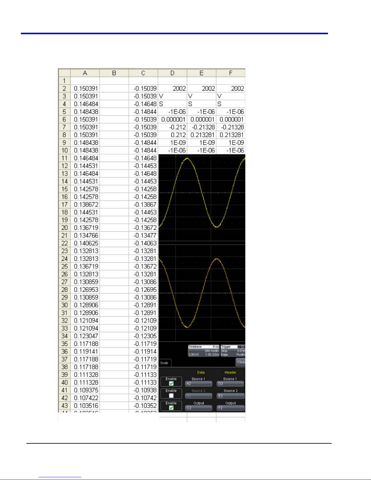
WavePro 7Zi
The input data are in columns A and B (though, only the first is used) and the output is in column C. All have been
set to start at row 2, allowing space for a title in row 1.
Columns D, E and F contain the headers for the three waveforms. These are the set of numbers that provide the
description of the scope settings, such as vertical scale and offset, and number of samples.
In this figure , the panel has been pasted
onto the Excel sheet for comparison:
77
WP700Zi-OM-E-RevA
Page 79
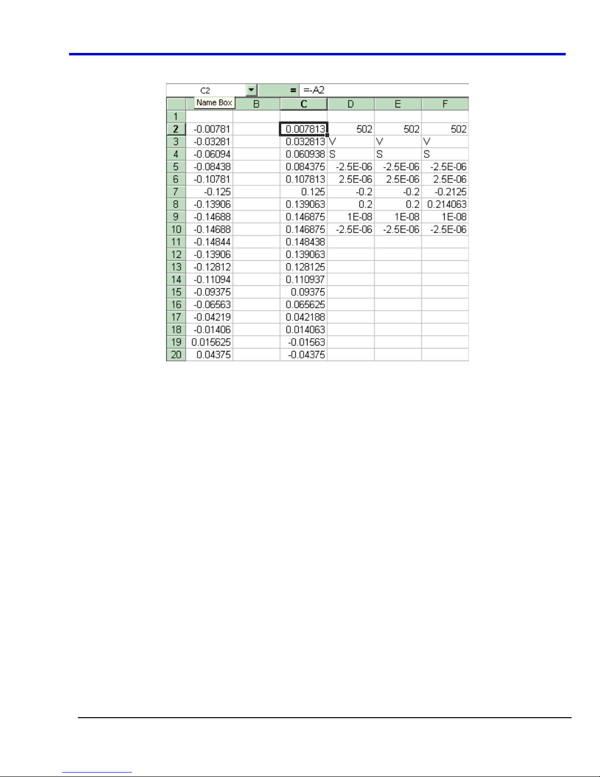
Operator's Manual
To get the output values in column C, we set C2 = - A2 and copy this formula down the column. This is the only
action needed in Excel, and can be seen in the next figure:
WP700Zi-OM-E-RevA
78
Page 80

WavePro 7Zi
Simple Excel Example 2
In this
example
we use Excel to invert or negate a waveform. The first figure shows a part of the instrument screen. The upper
trace (C1) is the original signal. The lower trace (F1) is the result calculated in Excel and displayed on the screen.
The input data is in columns A and B (though by default, only a single input/column is used), and the output is in
column C. All have been set to start at row 2 (which allows for a header in row 1).
To create this waveform, you would simply do the following:
1. Ensure that your acquisition has no more than 64 kpts (the Excel calculation limit)
79
WP700Zi-OM-E-RevA
Page 81

Operator's Manual
2. Choose a function, and select
ExcelMath as Operator1 for the
function. Excel will open automatically in the background.
3. Choose File, Minimize from the menu bar to minimize the instrument display and open the Excel
program.
4. Create your formula for each data point in column A (in this case, our formula for cell C2 is –A2,
copied for the entire column), as shown
here .
5. Retrigger the scope (if it is not currently triggering)
6. Return to the program
Note that the only action that was needed in Excel was to create the formula in column C for each data point in
column A. The instrument automatically opens Excel, puts the waveform data in the correct columns, and returns
the calculated data back to the display as the chosen F trace. This Excel-calculated trace can have further
measurements or math calculations performed on it, if desired.
WP700Zi-OM-E-RevA
80
Page 82

WavePro 7Zi
You can also create a chart of the data in
Excel automatically and view the data there. Simply press the Add Chart button in the instrument's Excel dialog
and a chart of the input (top chart) and Excel calculated output (bottom chart) will be automatically created in the
spreadsheet. The chart will be updated automatically as the scope is triggered.
81
WP700Zi-OM-E-RevA
Page 83
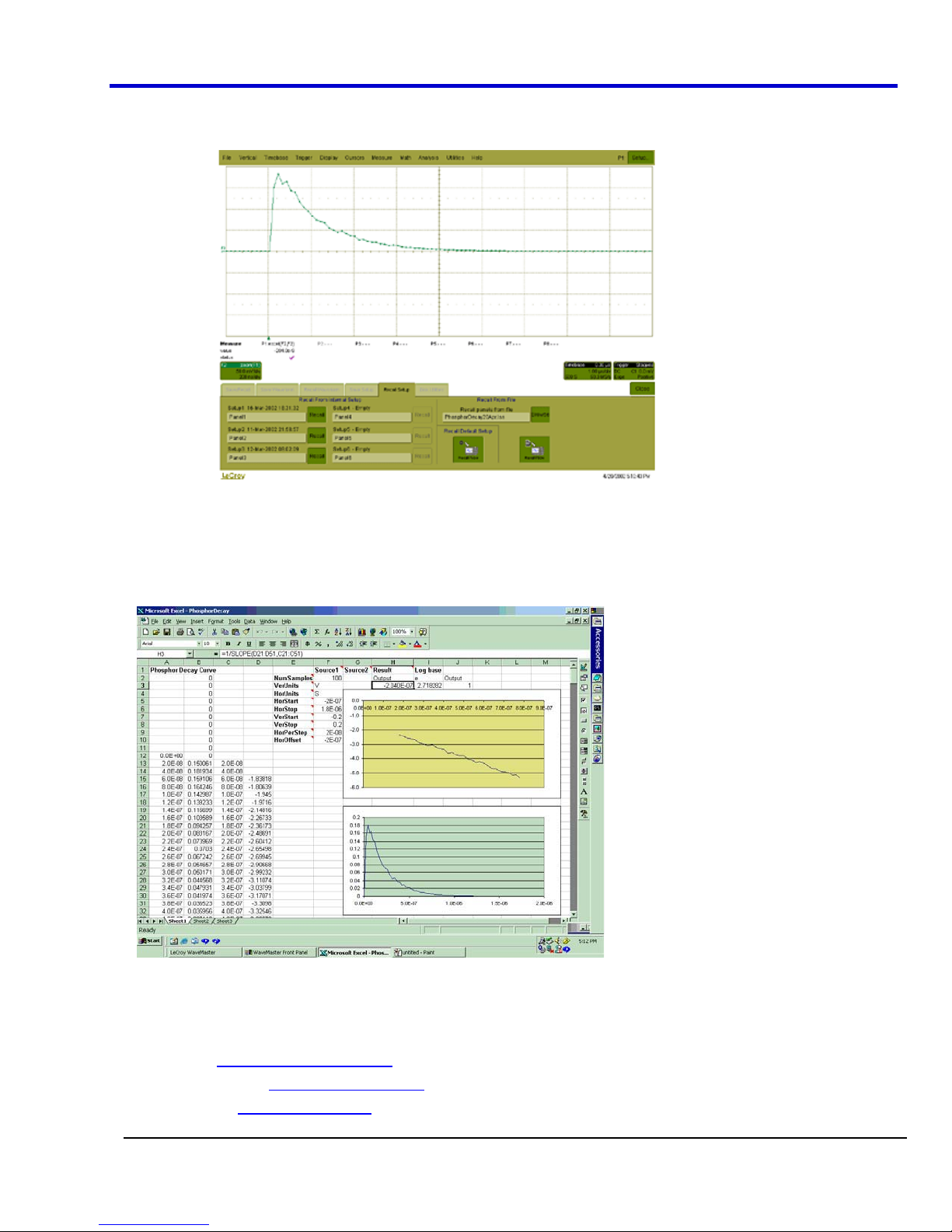
Operator's Manual
Exponential Decay Time Constant
This example calculates the time constant of an exponentially falling pulse, such as the light output of a phosphor.
The first figure shows a typical pulse, including
pseudo-random noise, generated by a VBScript.
The pulse was generated by a formula of the form e
requirement is to measure the time constant TC2, using the portion of the trace where TC1 has negligible effect.
This was done using Function F1, which is not a part of the measurement process.
For the actual measurement, Parameter P1 was set up as an Excel call. In Excel, the selected portion of the trace
was converted to logarithms, and the Excel function SLOPE was used, as shown
(1 – t/TC1)
* e
-t/TC2
, where TC1 and TC2 are time constants, The
here .
Here we see the input data in column B (with a time scale in A) created using the contents of cell F9, Horizontal
Per Step. The logarithmic data are in column D, with the time scale repeated in C. The output appears in cell H3,
using the formula =1/SLOPE(D21:D51,C21:C51).
Requred files:
Setup: PhosphorDecay20Apr.lss
F1 Generator: PhosphorPulseGen.txt
P1 Excel: PhosphorDecay.xls
WP700Zi-OM-E-RevA
82
Page 84

WavePro 7Zi
Gated Parameter Using Excel
This example calculates a parameter of a waveform, in a region of interest defined by the leading edges of two
pulses in a separate waveform.
This figure shows the instrument screen:
The traces were made using VBS scripts in functions F1 and F2, based on pseudo-random numbers to provide
noise and varying pulse widths. Randomize Timer:Randomize Timer was used in both scripts to ensure that
successive acquisitions produced different data. Script F1 generates pulses with widths that are multiples of a set
clock period. F2 generates one pulse in the first half of the time window, and one pulse in the second half. Both
pulses are constrained to coincide with the clock pulses of F1. F1 and F2 are used here only as simulations and
are not part of the measurement process, which only uses P1.
The call to Excel is made through Parameter P1.
The next figure shows a part of the Excel
workbook.
Here we see the gated waveform that has been created in Excel. The Mean parameter during the region of
interest (ROI) is placed in cell H3.
83
WP700Zi-OM-E-RevA
Page 85

Operator's Manual
How Does this Work?
The amplitude of the signal is about 0.3 volts, and the screen height is 0.4 volts, as derived from cells F7 and Fx.
A threshold value for amplitude was calculated by placing 0.5 * (Fy – Fx) in cell A4.
Remember that in the instrument the sources were defined to be A10 and B10. This means that the first point on
the waveform will be read into A10, and, since the waveform has 500 points, the last point will be read into A510.
The same holds true for F2 and column B, since F2 is assigned as Source2, and data is defined to write into
column B starting with cell B10.
To create the gating function in column C, the cell C10 was given the following formula:
IF ( ( B10 – B9) > $A$4, 1 – C9, C9). This was copied down the column. Column D, the output column, is simply A
* C.
The output was defined as cell H3.
The required mean in cell H3 is given by SUM (D10 : D509) / SUM (C10 : C509), for a 500 point waveform.
Requires files:
Setup: GatedParameterExcel.lss
Function F1: RandomPulses22Apr.txt
Function F2: RandomGate22Apr.txt
Parameter P1: GatedMean.xls
Correlation Excel Waveform Function
This example uses an Excel waveform
function to examine the cross-correlation between two signals, which are both noisy sinusoidal segments. The
correlation trace is, of necessity, shorter than the input traces.
The noise was generated using pseudo-random numbers. Randomize Timer was included in the VBScript to
ensure that the two traces differed, and that subsequent acquisitions differed. Functions F1 and F2 are included
only to simulate signals, and are not part of the measurement process, which is performed by F3.
WP700Zi-OM-E-RevA
84
Page 86

WavePro 7Zi
This example used the CORREL (Array1, Array2) function of Excel, as depicted below:
Required files:
Setup: CorrelateExcel22Apr.lss
Function F1:
Function F2:
Function F3:
NoisySine22Apr.txt
NoisySine22Apr.txt
Correlate22Apr.xls
Multiple Traces on One Grid
This example shows how you can place multiple traces in one picture, with only two operations in an Excel sheet.
Depicted below is an example from an Excel spreadsheet.
Here is an original instrument trace .
85
WP700Zi-OM-E-RevA
Page 87

Operator's Manual
The method is very simple. First, the waveform is transferred to an Excel spreadsheet by means of an instrument
Excel call. Second, two operations are needed in Excel: placing a simple formula in one cell, and copying that
formula into a range of cells.
Depicted below is the required Excel formula.
In fact, the simple expression B374 + 0.02 comprises several components. The original instrument trace is in
column B, and the plot is required to start at cell B134. The traces repeat at intervals of 250 cells. Let us call this
interval R. If we require a horizontal displacement D, then in cell CN we write B(N + R – D). In this example D is
10. Finally we may want a vertical displacement V, and we write B(N + R – D) + V. In this example, V is 0.02. D
and V can be zero if required, as depicted below. All that remains is to copy the formula to the required range of
cells.
WP700Zi-OM-E-RevA
86
Page 88

WavePro 7Zi
Required files:
F1 is needed only as a simulator of signals.
Instrument setup: LaserStartup25Apr.lss
Function F1: LaserStartupApr25.txt
LaserStartupPulses.xls
Function F2:
LaserStartupPulses2.xls
LaserStartupPulses3.xls
Using a Surface Plot
No offset
Vertical offset
Vertical and horizontal offset
87
WP700Zi-OM-E-RevA
Page 89

Required files:
Setup: LaserSurface1May.lss
Function F1 Generator: LaserSurface2May.txt
Function F2 Excel: LaserSurface2May.xls
Operator's Manual
Loading and Saving VBScripts
From the editing panel you can save your script and you can load a previous one. Should you forget to save a
script, please note that when you save your setup, it has your current scripts embedded in it. Therefore it is a
good idea to save your setup frequently. It is worth saving the script separately as well, because it is saved in a
suitable format for printing or off-line editing with Notepad. Note that in both these examples the input data are
referred to as InResult.DataArray. You can also write InResult1.DataArray and InResult2.DataArray, which refer
to the two input traces. InResult.DataArray always refers to input trace 1. These remarks hold for any script that
you write.
Example Waveform Function Script: Square of a Waveform
' Example script to produce a waveform
This example calculates the square of
the input waveform.
OutResult.Samples = InResult.Samples ' Visible trace length + 1
' Note that a trace of nominal length 1000 comprises data numbered from
' 0 to 1001. The 1001st point is not visible, so you
' normally use points 0 to 1000,
' giving 1001 points and 1000 intervals between points.
startData = 0
endData = OutResult.Samples
LastPoint = endData - 1 ' because the last point is invisible.
ReDim newArray(OutResult.Samples) ' to store the results
unscaledData = InResult.DataArray(False)
' InResult.DataArray(False) provides
' integer data from -32768 to 32767.
' InResult.DataArray(True) provides real data
' in the same physical unit as the vertical scale of the input trace.
ScaleFactor = 1.0 / 32768 ' to make the trace fill the screen.
For i = 0 To LastPoint
WP700Zi-OM-E-RevA
88
Page 90

WavePro 7Zi
newArray(i) = ScaleFactor * (unscaledData(i)) ^ 2
Next
OutResult.DataArray(False) = newArray ' signed long integer data output
Example Parameter Function Script: RMS of a Waveform
' Example script to produce a parameter.
' This script calculates the root mean square
' of the input waveform.
' Note that a trace of nominal length 1000 has data from
' 0 to 1001. The 1001st point is not visible, so you
' normally use points 0 to 1000,
' giving 1001 points and 1000 intervals between points.
startData = 0
endData = InResult.Samples
LastPoint = endData - 1 ' because the last point is invisible.
ReDim newArray(InResult.Samples) ' to store the results
unscaledData = InResult.DataArray(True)
' InResult.DataArray(False) provides
' integer data from -32768 to 32767.
' InResult.DataArray(True) provides real data
' in the same unit as the vertical scale of the trace.
Total = 0
For i = 0 To LastPoint
Total = Total + (unscaledData(i)) ^ 2
Next
NewArray(0) = Sqr (Total / (LastPoint + 1) Place the result in the zeroth element.
OutResult.ValueArray(True) = newArray ' integer data output
The Default Waveform Function Script: Explanatory Notes
InResult.Samples is the number of points in the incoming waveform.
InResult.DataArray(Boolean) (or InResult1.DataArray or InResult2.DataArray) is the array of input data. If the
Boolean is True you get scaled real data in the units of the trace. If the Boolean is false you get unscaled integer
data in the range -32768 to + 32767.
The value of InResult.Samples is the total number of data in a trace. It is two more than the nominal value given
on the screen. The first point DataArray(0), coincides with the left edge of the screen, apart from the wobble
caused by the trigger-to-sample clock difference. If the trace length is nominally 500, the right edge of the screen
coincides with DataArray(500), which is the 501
screen, and is never seen. That is why the loop in the script runs only to endData - 1.
OutResult.Samples is the number of data in the output trace, and is set to be the same as the number of data in
the input trace. If you set the output length less than the input length, you get a shorter trace, the remainder being
made of zeroes. If you try to set the output values to something illegal, you may find that a part of the trace retains
the values from a previous acquisition.
If you try to set something outside the bounds of an array, or you make some other error, or something overflows,
or you ask for something impossible, such as log(-13), the instrument tells you the line number, and the nature of
the problem. Other types of error may not be given the correct line number, for example, if "Next" or "End If" is
omitted, because VBS does not know where it should have been.
UnscaledData is simply a copy of the input data set.
ReDim newDataArray(OutResult.Samples) defines an array of data for use as a scratch pad. Dim is short for
Dimension, which is used in Visual Basic to declare a variable (even if it only has one element, in which case you
omit the size of the array).
st
point. The last point, number 502, is just off the right of the
89
WP700Zi-OM-E-RevA
Page 91

Operator's Manual
InResult.DataArray(False) means that the data are signed integers in the range -32768 to 32767. False is a
Boolean value applying to the property Scaled. Scaled data are specified in the units of the vertical scale, such as
volts. You get these by putting "True" instead of "False". If you want to make a section of the output trace
invisible, you simply set the data values to full scale or bigger, top or bottom.
You can start with the unscaled data (False) as input, and then set the output data to scaled data (True), and you
can go from scaled to unscaled. Using scaled data, an overflow will make a picture like this:
You can also start with True and convert to False, but in this case overflows will cause an error message.
Anything after a single quotation mark on a line will not be used by the instrument. This feature is intended for
comments, for example
' This is a comment.
A = Amp * Sin(Omega * T) Calculate the output.
InResult.DataArray and OutResult.DataArray are only to be used as shown in the default scripts and in the
example scripts: you cannot refer directly to individual elements of these arrays. You have to use your own
arrays, in this example, unscaledData and newDataArray. You are not allowed to write statements like the
following:
Y = InResult.DataArray (17)
OutResult.DataArray (257) = Z
Some parts of the default script must not be changed because they are a part of the interface. These are
highlighted in the following script .
' TODO add your custom code here accessing OutResult and InResult objects
' Here's a small example that just inverts the waveform.
OutResult.Samples = InResult.Samples
startData = 0
endData = OutResult.Samples
newNumPoints = endData - startData
ReDim newDataArray (OutResult.Samples)
unscaledData = InResult.DataArray (False)
For i = 0 To endData - 1
newDataArray (i) = - unscaledData (i)
Next
OutResult.DataArray (False) = newDataArray ' only support raw data
The four highlighted quantities are parts of the interface. The names must be retained. Furthermore,
InResult.Samples and InResult.DataArray are inputs, and their values cannot be changed. OutResult.Samples
and OutResult.DataArray are outputs, and can be changed, but not directly through their individual elements.
WP700Zi-OM-E-RevA
90
Page 92

WavePro 7Zi
Default Parameter Function Script
The default parameter script is similar to the default waveform script, but there are subtle differences.
First, the size of the data array is the same as the nominal value: you cannot use or see the extra two points. So
"500 points" means just that: 500 points.
Second, the output looks like an array, but only element zero is currently used. You must copy your parameter result into newValueArray(0).
As with the arrays of the Waveform Script, you cannot refer directly to elements of the input and output arrays. You may not write something
like
OutResult.ValueArray (0) = P.
Note that the unit of the parameter is displayed as the same as the vertical unit of the trace, even if you have
squared the data, for example, unless you change the unit yourself.
To find out how to edit a parameter script, click here
The default parameter script is shown below.
' TODO add your custom code here accessing OutResult and InResult objects
' Here's a small example that just inverts the waveform
numParam = InResult.Samples
ReDim newValueArray(numParam)
scaledData = InResult.DataArray
For i = 0 To numParam-1
newValueArray(i) = -scaledData(i) ' Change this to do something useful.
Next
OutResult.ValueArray = newValueArray 'only support raw data
Your parameter script should include something like this:
A. Do calculation to obtain your parameter value from the input data array.
B. newValueDataArray (0) = ParameterValue
C. OutResult.ValueArray = newValueArray
You can test this script using setup MeanDemoScriptApr2.lss
You can edit scripts using Notepad, but you will not get any notification of errors.
You are not
allowed to write OutResult.ValueArray(0) = MeanParameter.
InResult.DataArray and OutResult.DataArray are only to be used as shown in the default scripts and in the
example scripts. You cannot refer to, or modify, any individual element in these arrays.
.
.
Hints and Tips for VBScripting
x Set the trigger to Single or Stopped if you need to do a lot of editing: it is faster.
x Before starting a script, remove any existing scripts that you do not need. This is because errors in an
existing script will give you error messages, even if your current script is perfect. And an existing good
script may develop a fault if you change the setup. For example, you might change the vertical scale or the
memory length and get an overflow if you did not guard against it in the script.
x When starting a script, make sure that you have chosen the right kind: function or parameter. You can get
some very frustrating problems if you are in the wrong mode. You can cut and paste the VBS statements if
you discover this error.
x If your calculation requires a long memory, development might be quicker if you test the principles on a
shorter trace at first.
x Note that the pseudo-random number generator is reset at the start of a script. If you want a different set of
pseudo-randoms every time, put Randomize Timer in the program, to be run once, before any pseudorandoms are generated. You can use this instruction to re-seed the generator at any time during execution.
x Do not put the final statement in a loop, hoping that you can see a progressive result as some parameter
changes. No output will be seen on the screen of the instrument until the script has been completely run
and quitted, so only the final result will appear. If the loop runs many times, you will think that the scope
has hung up.
x If you want a For loop, end it with "Next" and not "Next X".
91
WP700Zi-OM-E-RevA
Page 93

Operator's Manual
x If you make a script that takes a long time to run, go back to the default setup before quitting or powering
down, or you will have a long wait next time you power up.
x Always use a recursive calculation when this will speed things up.
x Keep everything outside a loop that does not have to be inside, to speed things up.
x Make your scripts clear, not only by indenting and commenting, but by structuring neatly as well.
x Sometimes it might be easier to develop your script in Excel VBA (remembering that VBA is not identical to
VBS), so that you can display intermediate results. If you do this, note that you can read from a cell or write
to it using statements like these:
A = Worksheets("Sheet1").Cells(Row, Column).Value
Worksheets("Sheet1").Cells(Row, Column).Value = B
x Note that in VBS, after you have corrected an error and clicked on "Apply," the error message may go on
flashing for a few seconds, or a few acquisitions, before being erased. Look for the "Script OK" message.
Be patient before assuming that you still have a bug.
x If your calculation requires data to be used at some other horizontal positions than their original ones,
make sure that your algorithm does not try to send data to non-existent array positions, that is, beyond the
edges of the screen. You may have to truncate your output trace, as happens with the instrument's
Enhanced Resolution and Boxcar functions.
x No output will emerge from a script until you press Apply.
x No output will emerge from a script until it has received an input. This includes the case where the input
data are not used in calculating the output data. So you must have had at least one acquisition before you
see anything.
x Because you can introduce undeclared variables at any point in a calculation, VBS does not check your
spelling.
x You can make a portion of a trace disappear if you set the values to 32767 or -32768.
x You can highlight a section of a trace by making the points alternately too high and too low by a suitable
amount. Providing the memory length is not too short, the compaction algorithm will give the effect of a
thicker trace.
x The lengths of the output trace and the input trace need not be the same. You can even make the output
trace longer than the input trace, but you will need to unzoom it to see it all. This feature can be used to
avoid compaction problems with non-linear horizontal scales. It can also be used to show several versions
of a function at the same time, without having to set up a separate script for each one.
x If your program structure is complicated, consider typing all the IFs, ELSEIF's, ENDIF's, FOR's, NEXT's,
etc and then clicking Apply. You wont get any output, but the system will tell you if the structure is
acceptable. Then you can insert the actual program statements.
x Always try to make the script as independent as possible of variables such as V/Div, T/Div, and memory
length, unless that would make it harder to understand. If so, give some values as examples, and explain
how the script would have to change if the variables changed.
Errors
The instrument VBS tries hard to help you when errors occur.
Errors may be of two main types:
x The script may not be usable because the interpreter cannot construct a logical structure from it.
x The script may be usable, but may fail while running because an incomputable function has been
requested.
Sometimes the line number given for an error is wrong. This can happen when the error is of this general type:
Missing "Next" Missing "End If"
Extra "Next" Missing "Until" etc.
This happens because VBS cannot know where you should have put the statement.
If at some point during the calculation of an output array, a value goes outside the allowed range, the calculation
will stop, and you will see the new values up to the point of the stoppage. To the right of that point, the trace will
display the previous values. In fact, if you deliberately recalculate only a part of a trace, you can have a mixture of
new and old values.
WP700Zi-OM-E-RevA
92
Page 94

WavePro 7Zi
In the figure below is a type of error message that you may see if one of your calculations has tried to set a value
outside the range -32768 to +32767. It takes extra time to guard against this, but unless you are sure that it will
not happen, you need some kind of check. In the example on the next page, the red trace has gone outside the
allowed range at the beginning, resulting in the message at the bottom of the instrument screen: This array is
fixed or temporarily locked: OutResult.DataArray.
Error Handling
Note that the construction OnError GoTo Label: is not allowed in VBS. In fact no GoTo's or labels are allowed.
Therefore there is no way for you to provide handlers to deal with errors and exceptions. You must be aware of all
possibilities at all points in your program, and you must either be certain that errors will not occur, or you must
take action to ensure that they do not.
Examples:
Function:Description:
Sqr
Log
A / B
Array
Size
If there is any possibility that any of these might occur, take steps to deal with this before it can happen.
For example, you may write some kind of generator of pseudo-random statistical values. If these belong to a
distribution that in principle has an infinite range, or a finite range which is wider than the signed 16-bits allowed,
check each value. If a value falls outside the range, you could set it to the maximum or generate another
example.
You cannot take the square root of a negative number.
You cannot take the log of zero or of a negative number.
You cannot divide by zero.
You cannot use an index outside the bounds of an array.
Unscaled data cannot go outside the range -32768 to 32767.
93
WP700Zi-OM-E-RevA
Page 95

Operator's Manual
You can, however, use one of the following:
On Error Resume Next
followed by some code that may make some attempt to deal with the problem, or at least to allow execution to
continue.
On Error GoTo 0
This cancels On Error Resume Next
Speed of Execution
To maximize the speed of execution of a script, the most important thing you can do is to minimize the number of
operations that are performed inside loops. Anything done once only is unlikely to be an important source of
delay. Please note that VBS is much slower than the internal computations of the instrument, so do everything
you can to save time, unless time is irrelevant to the application.
Using an array element takes longer than using a single variable. Here is an example:
For K = 1 to Total
If X (K) > X (K - 1) Then
Y = Cos (X (K) ) * Sin (X (K) ) * Sqr (X (K) )
End If
Next
To do the same thing we could also write this, using the index only once:
OldXK = X (0)
For K = 1 To Total
XK = X (K)
If XK > OldXK Then
Y = Cos (XK) * Sin (XK) * Sqr (XK)
OldXK = XK
End If
Next
VBS runs slower than the "internal" calculations, because the scripts are interpreted. This could be serious for
calculations where many operations are needed on each sample, such as convolution, correlation, and long
digital filters.
Scripting Ideas
What can we do in a VBS script that we cannot do with the normal instrument functions? Here are some
possibilities.
x Create a new function that acts on waveform values.
x Create a new parameter.
x Create a new form of non-linear vertical scale.
x Create a new form of non-linear horizontal scale.
x Move some or all data horizontally, including reflections.
x Combine data to form digital filters.
x Show several function results side by side.
x Show several function results interleaved.
You can even create output data that are not related to the input. The output data need not even be in the same
domain as the input data, because the system treats them as pure numbers. So you can create your own
transforms into the frequency domain, for example.
Example Waveform Script
Creating a window function for FFT calculations.
WP700Zi-OM-E-RevA
94
Page 96

WavePro 7Zi
Example Parameter Script
Calculating the rate of decay of a damped sine.
Finding pulses in a pulse train.
Debugging Scripts
Until we have integrated a more comprehensive debugger for VBScript there is a workaround.
1. Download the Windows Scripting Debugger for Windows 2000 from here:
http://download.microsoft.com/download/winscript56/Install/1.0a/NT45XP/EN-US/scd10en.exe
2. Enable JIT (Just In Time) debugging by setting the following registry key
HKCU\Software\Microsoft\Windows Script\Settings\JITDebug = to 1 (DWORD value)
3. Place a Stop statement in your script.
Now, when the Stop statement is executed the debugger will open and allow single-stepping, variable
examination, etc.
Using VBA or Visual Basic to debug VBScripts is not recommended since the language syntax for these three
variants of basic is slightly different.
Calling MATLAB from the Scope
Note: Load MATLAB version 6.5 just as you would on any PC. Once it is loaded, open MATLAB from the
desktop, then close it again, before you attempt to open it from the instrument application. This is to update the
registry.
MATLAB can be directly called from the instrument in two ways:
Calling MATLAB: Description: Result:
Using a
function
Using a
parameter
In both cases, one call to MATLAB can use two separate waveforms as input, providing much greater computing
power than is available by calling MATLAB from a VBScript.
Note: If you do not place a semicolon ";" at the end of a line, MATLAB will show the calculated value in the result
window, significantly slowing down the processing rate. This feature is best kept for diagnostics.
F1 through Fx[The number of math traces available depends on the software
options loaded on your scope. See Specifications.]
P1 through Px
MATLAB returns a
waveform
MATLAB returns a
parameter
95
WP700Zi-OM-E-RevA
Page 97

Operator's Manual
Selecting a Waveform Function Call
The MATLAB Waveform functions are selected from the Select Math Operator menu. Please note that once you
have clicked on "MATLAB Wave" there will be a slight pause before MATLAB starts.
Figure 4-6. Source 1 and Source 2 are the waveforms that MATLAB will use.
WP700Zi-OM-E-RevA
96
Page 98

WavePro 7Zi
MATLAB Waveform Control Panel
Once you have invoked a MATLAB waveform call, you will see the zoom dialog at the right of the screen. Touch
the MATLAB tab to see a panel like this .
Touch Find Scale to make your output fit the grid, or use the text boxes to choose a scale.
MATLAB Waveform Function Editor
By touching Edit Code, you can reach the MATLAB Editor where you will see the default waveform function. If
you are familiar with MATLAB, you might prefer to launch MATLAB and create a MATLAB function that performs
your task. Your program in the instrument could then be a one-line call of your MATLAB function.
97
WP700Zi-OM-E-RevA
Page 99

Operator's Manual
This is the default waveform function, with one important change – the semi-colon (;) has been removed from the
end of the line. If the semicolon is present, your function will run much faster, because the output values will not
be shown in MATLAB Response. With a long waveform, the time needed to display it could be quite long. The
response values can be useful during development and debugging. Any line without a semicolon will produce a
visible MATLAB Response.
From this panel you can save your code, load a previous code, and edit your function. A powerful feature of
MATLAB is that you can refer to an entire waveform as a vector. The two input waveforms are WformIn1 and
WformIn2, while the output is WformOut. You can also refer to individual samples, such as WformIn1(34), and
sequences of samples, such as WformIn(55:89)
You can write statements such as these:
WformOut(5) = WformIn(5)
WformOut(89) = WformIn(144)
WformOut(34:55) = WformIn(34:55)
WformOut(233:377) = WformIn(100:244)
Figure 4-7. This very simple example adds a rescaled copy of Channel 2 to a copy of Channel 1, and then
rescales the result.
WP700Zi-OM-E-RevA
98
Page 100

WavePro 7Zi
MATLAB Example Waveform Plot
If you touch the MATLAB Plot checkbox you will see a MATLAB plot like this
one .
99
WP700Zi-OM-E-RevA
 Loading...