Leader LBO-516 User Manual

Page 1

Page 2

WARNING!

THE SERVICING INSTRUCTIONS CONTAINED IN THIS MANUAL ARE FOR USE BY QUALIFIED PERSONNEL ONLY. TO AVOID ELECTRIC SHOCK, DO NOT PERFORM ANY SERVICING OTHER THAN THAT CONTAINED IN THE OPERATING INSTRUCTIONS UNLESS YOU ARE QUALIFIED TO DO SO.

Page 3

LBO-516 100 MHz

DELAYED TIME BASE OSCIILOSCOPE

TABLE OF CONTENTS

1. GENERALINFORMATION

1-1 INTRODUCTION ................................................................................................................................1

1-2 SPECIFICATIONS ..........…..................................................................................................................................1

2. OPERATING INSTRUCTIONS

2-1 FUNCTION OF CONTROLS, CONNECTORS, AND INDICATORS .......................................................... 3

2-1-1 Display Block ........................................................................................................................................... 3

2-1-2 Vertical Amplifier Block ........................................................................................................................... 4

2-1-3 Sweep and Trigger Blocks ......................................................................................................................... 5

2-1-4 Miscellaneous ........................................................................................................................................... 7

2-2 INITIAL OPERATION ................................................................................................................................ 7

2-2-1 Power Connections and Adjustments ......................................................................................................... 7

2-2-2 Installation ................................................................................................................................................ 8

2-2-3 Preliminary Control Settings and Adjustments ........................................................................................... 8

2-3 BASIC OPERATING PROCEDURES ......................................................................................................... 9

2-3-1 Signal Connections ................................................................................................................................... 9

2-3-2 Single-trace Operation ..............................................................................................................................11

2-3-3 Triggering Alternatives ............................................................................................................................11

2-3-4 Probe Compensation ................................................................................................................................14

2-3-5 Dual-trace Operation ................................................................................................................................15

2-3-6 Additive and Differential Operation ..........................................................................................................16

2-3-7 Triple-trace Operation ..............................................................................................................................17

2-3-8 Four-trace Operation ................................................................................................................................17

2-3-9 Delayed Timebase Operation ....................................................................................................................18

2-3-10 Single-shot Operation .............................................................................................................................20

2-3-11 X-Y Operation .......................................................................................................................................20

2-3-12 Intensity Modulation ..............................................................................................................................20

2-4 MEASUREMENT APPLICATIONS ...........................................................................................................21

2-4-1 Amplitude Measurements .........................................................................................................................21

2-4-2 Differential Measurement Techniques .......................................................................................................22

2-4-3 Time Interval Measurements ....................................................................................................................23

2-4-4 Phase Difference Measurements ...............................................................................................................24

2-4-5 Distortion Comparison .............................................................................................................................26

2-4-6 Frequency Measurements .........................................................................................................................27

2-4-7 Risetime Measurements ............................................................................................................................27

2-4-8 -3dB Bandwidth Measurement ..................................................................................................................28

........................................................................................................................................1

..................................................................................................................................3

Page 4

1. GENERAL INFORMATION

1-1. INTRODUCTION

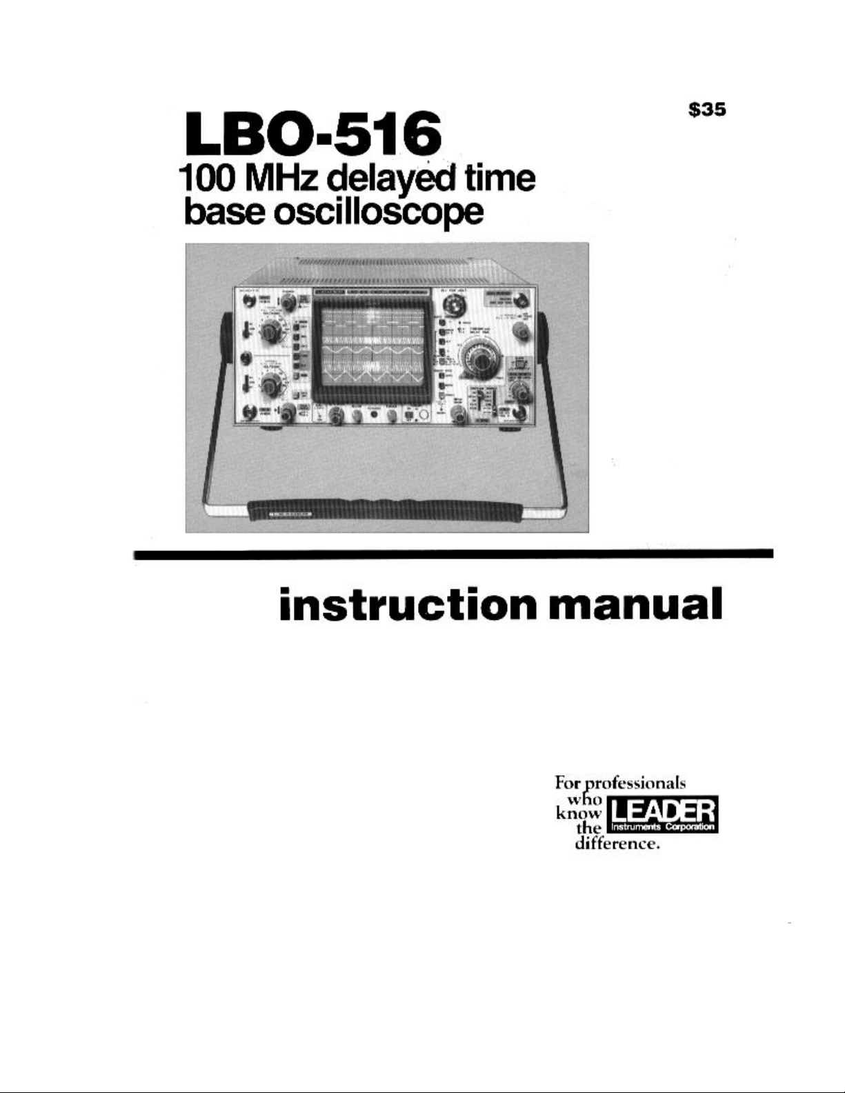
The LBO-516, shown in Figure 1-1, is a 100 MHz oscilloscope

with all of the features normally found on a lab-grade scope: highfidelity pulse response, stable operation, dual timebase with calibrated sweep delay, flexible triggering facilities, and a bright CRT display with illuminated internal graticule. Moreover, it also has a very unusual feature found on few scopes in any price class: it can simultaneously display up to eight traces from three different input signals! In addition to the two vertical-input channels and their difference signal, the signal used to externally trigger the main timebase can also appear on the CRT display. The alternate sweep mode, which allows the main and delayed timebases to simultaneously sweep the CRT, effectively doubles this four-trace display to an eight-trace display.

The comprehensive triggering facilities of the LBO-516 include

several features that ease the problem of triggering on complex signals: a variety of frequency-selective coupling filters, a trigger holdoff-control, and a trigger pickoff that alternates between the two vertical channels.

1-2. SPECIFICATIONS

Specifications for the model LBO-516 oscilloscope are given in

Table 1-1.

Table 1-1

SPECIFICATIONS

Vertical Amplifiers (Ch. 1 & 2)

Bandwidth (-3 dB) DC coupled DC - 100 MHz AC coupled 10 Hz - 100 MHz Rise Time 3.5 KS Deflection Coefficients

Accuracy 5 mV/div to 5 V/div in 10 calibrated

steps, 1-2-5 sequence. Continuously variable between steps. XI0 magnification adds 0.5, 1, and 2 mV/div steps for frequencies below 5 MHz

Input Impedance -+3%; -+5% with Xl0magniflca-tion

1 megohm +-2%, 25 pF +-3 pF

Maximum Input Voltage 400 V (DC plus AC peak)

Page 5

Signal Delay Leading edge displayed. Leading edge displayed. CH-1 only, CH-2 only,

CH-1 & CH-2 displayed alternately, CH-1 & CH-2 chopped (at 250 kHz rate), CH-1 & CH-2 added, CH-1 & CH-2 subtracted, CH-1 & CH-2 & CH-3 displayed alternately, CH-1 & CH-2 & CH-3 chopped, CH-1 & CH-2 & CH-3 & CH-1 + CH-2 alternated, CH-1 & CH-2 & CH-3 & CH-1 + CH-2 chopped, CH-1 & CH-2 & CH-3 & CH-1

- CH-2 alternated, CH-1 & CH-2 & CH-3 & CH-1

- CH-2 chopped.

Common Mode Rejection 20dB at 20MHz CH- 1 Output 25 mV/div into 50 ohms

Horizontal Amplifier (X-Y Mode)

Bandwidth (- 3 dB) DC coupled DC - 3 MHz AC coupled 10Hz - 3MHz Rise Time 120 KS

Phase Shift <3° at 100 kHz Deflection Coefficients 0.5 mV/div to 5 V/div in 13 calibrated

steps, 1-2-5 sequence, continuously variable between steps

Accuracy +-3% for 5 mV/div to 5 V/div,

+-5% for 0.5 mV/div to 2 mV/div Input Impedance 1 megohm -+2%, 25 pF +-3 pF Maximum Input Voltage 400 V (DC plus AC peak)

Time-Base Generators

Display Modes Main timebase (TB) only,

Main TB intensified by delayed

TB,

Delayed timebase,

Main TB alternated with

delayed TB. Main (A) Time Base 0.02 KS/div to 0.5 S/div in 23

calibrated steps, 1-2-5 sequence.

Continuously variable between steps. Delayed (B) Time Base 0.2 PS/div to 50 mS/div in 20

calibrated steps, 1-2-5 sequence. Magnifier XI0 deflection increase at any TB

setting extends sweep speeds of main

and delayed TB's to 2 KS/div. Accuracy +- 3% unmagnified

+- 5% magnified Delay Time Continuously variable multiplier with

1000 divisions. Delayed TB Jitter 1/20,000

Trigger Circuits

Sources CH-l, CH-2, Alternate, Line, External

Modes Auto, Normal, Single-shot Coupling AC, DC, HF reject, TV vertical, TV

horizontal Slope + orHoldoff Normal, Variable (to greater than

one sweep), B ends A Sensitivity Internal Trigger DC – 10 MHz: 0.4div

External Trigger DC - 10MHz: 100mV

External Trigger Amplifier (Ch. 3)

Bandwidth (-3 dB) DC coupled DC - 100 MHz AC coupled 10Hz- l00 MHz Rise Time 3.5 KS Deflection Coefficients 0.2 V/div and 2 V/div Accuracy +-3% Input Impedance 1 megohm +-2%, 30 pF Maximum Input Voltage 400 V (DC plus AC peak)

Z-Axis Modulation

Level for Blanking Standard TTL high (+ 2 to + 5V) Coupling DC Maximum Input Voltage 50 Vp-p Input Impedance 10k: Bandwidth DC-5 MHz

Calibrator

Output Voltage 500 m Vp-p--+ 2%, positive-going,

Frequency 1 kHz nominal Waveform Fast-rise rectangular wave

CRT Display

Phosphor P31 (P39 optional) Accelerating Potential 20 kV/2kV Graticule Internal 1 cm square divisions, 8 div

Graticule Illumination Continuously variable Trace Adjustments on Rotation, focus, intensity,

Front Panel B intensity

Other Features

"Out-of-Calibration" Indicator Other Indicators Main timebase triggered

Power Requirements

Line Voltage 100/120/200 VAC 220/240 VAC

Line Frequency 50-60 Hz Power Consumption 55W

Physical & Environmental Data

Case Size (WxHxD) 12.3 x 5.8 x 16 inches 305 x 145 x 400 mm Overall Size (WxHxD), 13.75 x 7.25 x 18.5 inches handle folded back 350 x 185 x 470 mm

10 - 100 MHz: 1.5 divs

10 - 100 MHz: 400mV

ground referenced

high, 10 div wide.

Central axis subdivided into 0.2 cm

graduations.

Main timebase

Single-shot ready

Power on



Page 6

3 4 5 6 7 8 9

Weight 20.9 lbs, 9.5 kg Ambient Operating 0-40°C (32-104°F) maximum Temperature 15-35°C (60-95°F) for guaranteed

specs

Vibration Tolerance 2 mmp-p displacement at 12-33 Hz

and 33-35 Hz

Shock Tolerance 30g

Accessories

Supplied Instruction Manual

Two (2) LP- 100X probes Two (2) BNC-to-post adaptors

Optional LP-2017 Probe Pouch

LC-2016 Protective Front Cover LR-2402 Rack Mount Adaptor LH-2015 Hood

Specifications for the model LP-100X scope probe are given in

Table 1-2.

2. OPERATING INSTRUCTION

This section contains the information needed to operate the LBO-516 and utilize it in a variety of basic and advanced measurement procedures. Included are the identification and function of controls, connectors, and indicators, initial startup procedures, basic operating routines, and selected measurement applications.

2-1. FUNCTION OF CONTROLS, CONNECTORS, AND

INDICATORS

Before turning on

controls, connectors, indicators, and other features described in this section. The descriptions given below are keyed to the items called out in Figures 2-1 to 2-4.

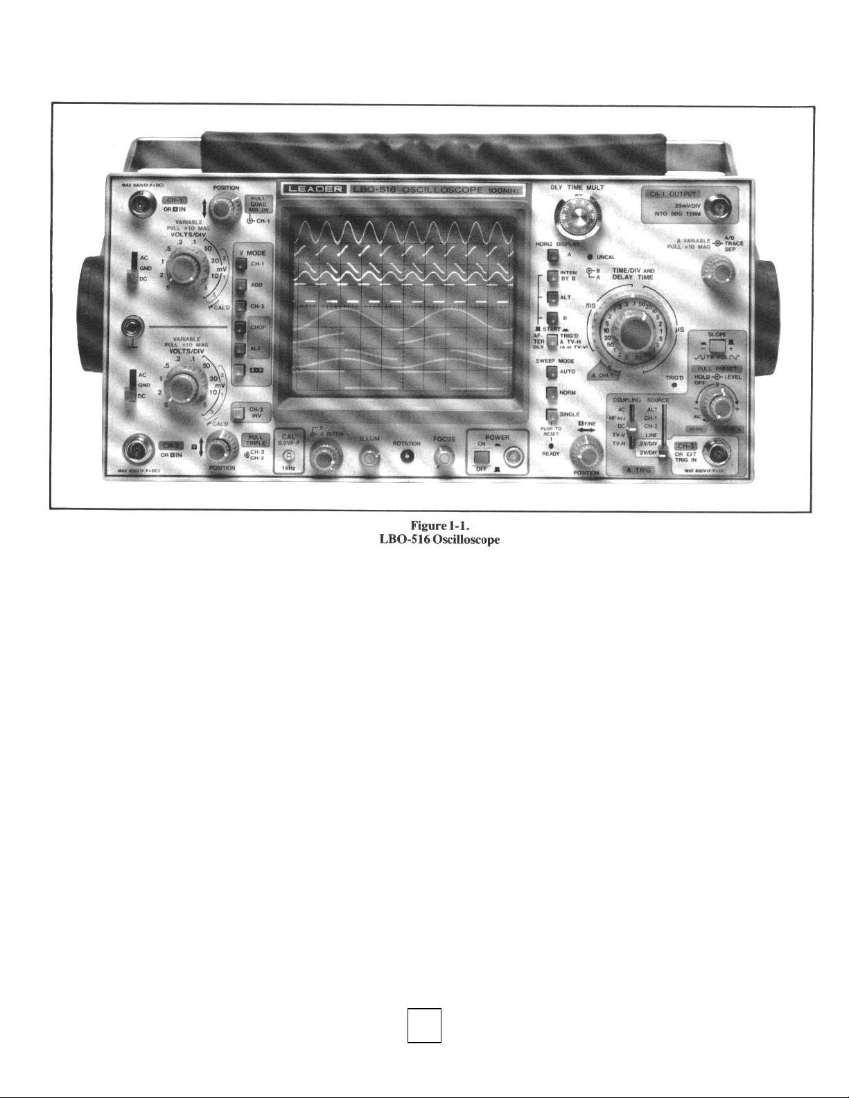
2-1-1 Display Block

Refer to Figure 2-1 for reference (1) to (9).

POWER switch Push in to turn instrument power on

POWER lamp Lamp lights when power is on

A INTEN control To adjust the overall brightness of the

B INTEN control Provides adjustment of CRT brightness

FOCUS control To attain maximum trace sharpness.

ROTATION control Provides screwdriver adjustment of

this instrument, familiarize yourself with the

and off

CRT display. Clockwise rotation increases brightness

during INTEN BY B interval and B timebase sweeps

Astigmatism is automatically adjusted.

horizontal trace alignment with regard to the CRT graticule lines

Table 1-2

Attenuation Ratio 10:1 +-2% and 1:1, switch selectable Input Impedance 10X attenuation 10 megohms, 12 pF + 1X attenuation Scope input Z plus < 150 pF Rise Time (10X atten.) 3.5 KS nominal Overshoot & Ringing <10%

(10X atten.) Bandwidth 10X attenuation DC- 100MHz 1X attenuation DC - 6 MHz Maximum Input Voltage 600 V (DC plus AC peak) Ambient Operating Temperature Maximum - 10 to + 55°C For guaranteed

Specifications +5 to +35°C Ambient Humidity Maximum 40 to 90% For guaranteed

Specifications 45 to 85%

CRT Display device having 1 cm square

ILLUM control To adjust graticule illumination. Clockwise rotation increases brightness CAL connector Provides fast-rise waveform of precise

LP-100X SPECIFICATIONS

10%

graticule lines inscribed on the inner CRT surface for parallax-free measurements. Blue filter provides good contrast and pleasing display.

amplitude for probe adjustment and vertical amplifier calibration.

Page 7

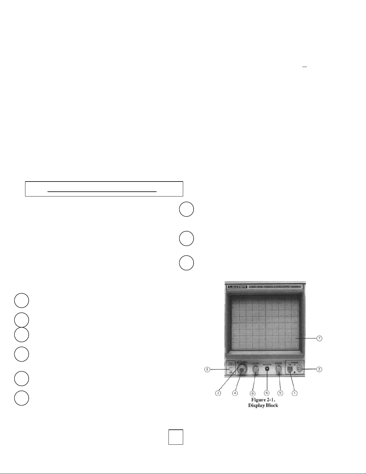
2-1-2 Vertical Amplifier Block

11 23 22 12

13 14

16 17 18 19 20 21

Refer to Figure 2-2 for references (10) to (12) and (14) to (23).

Refer to Figure 2-3 for reference (13).

VOLTS/DIV switches To select the calibrated deflection

factor of the input signals fed to the vertical amplifier.

VARIABLEcontrols Provide continuously variable

adjustment of deflection factor between steps of the VOLTS/DIV switches. Calibrations are accurate only when the VARIABLE controls are detented in

PULL X 10 MAG Pulling these out will increase the (on VARIABLE sensitivity of the associated vertical controls) amplifiers by ten times at reduced

Ground Connector Provides convenient point to attach

CH-1 OUTPUT Provides scaled output of the channel 1 Connector signal suitable for driving a frequency

CH- 1 or X-IN For applying an input signal to vertical connector amplifier channel 1, or the X-axis

CH-2 or Y-IN For applying an input signal to vertical connector amplifier 2, or the Y-axis (vertical)

AC/GND/DC To select the method of coupling the switches input signals to the vertical amplifiers.

Channel 1 Vertical For vertically positioning trace 1 on the POSITION control CRT screen. Clockwise rotation moves

Channel 2 Vertical or For vertically positioning trace 2 on the Y POSITION control CRT screen. Clockwise rotation moves

CH-2 INV switch Push in to invert the polarity of the

X-Y switch Push in to select X-Y operation.

V MODE switches To select the vertical amplifier display

their fully clockwise positions.

bandwidth.

separate ground lead to oscilloscope.

counter or other instrument.

(horizontal) amplifier during X-Y operation.

amplifier during X-Y operation.

AC position connects a capacitor between the input connector and its associated amplifier circuitry to block any DC component in the input signal. GND position connects the amplifier input to ground instead of the input connector, so a ground reference can be established. DC position connects the amplifier inputs directly to the associated input connector, thereby passing alt signal components on to the amplifiers.

the trace up. Inoperative during X-Y operation.

the trace up. Adjusts the Y-axis of the trace during X-Y operation.

Channel 2 signal.

CH-1

mode. the input signal of channel 1 on the CRT when pressed

push-button displays only

Figure 2-2

Vertical Amplifier Block

CH-2

push-button displays only the input signal

of channel 2 on the CRT when pressed.

ALT

push-button displays the input signals of both channels 1 and 2 (or more) on the CRT when pressed. The CRT beam is switched between channels at the end of each sweep to achieve this multi-channel display.

CHOP

push-button displays the input signals of both channels 1 and 2 (or more) on the CRT when pressed. The CRT beam is switched between channels at a 250 kHz rate during the horizontal sweep to achieve this multi-channel display.

ADD

push-button displays a single trace that is the algebraic sum of the input signals of channels 1 and 2 when pressed.

PULL TRIPLE control When pulled, displays traces for CH-1,

CH-2, and CH-3 (trigger), providing ALT or CHOP push-button is also pressed. Rotating this control also vertically positions the CH-3 trace on the CRT screen. This control is not operative if any single-trace display mode is selected.

PULL QUAD control When pulled, displays traces for CH-l,

CH-2, CH-3 (trigger), and algebraic sum of CH-1 and CH-2 signals, providing ALT of CHOP pushbutton is also pressed. This control is not operative if any single-trace display mode is selected.

Page 8

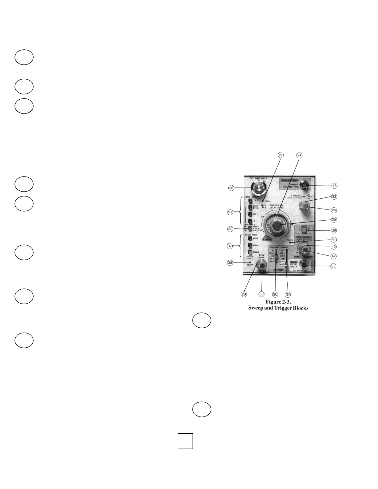
2-1-3 Sweep and Trigger

24 32 25 26 27 28 29 30 31 33

Refer to Figure 2-3 for reference (24) to (42).

ATIME/DIV and To select either the calibrated DELAY TIME sweep of the main (A) time-base switch or the delay time range for delayed sweep operation.

B TIME/DIV switch To select the calibrated sweep rate of

A VARIABLE/ Provides continuously variable PULL X 10 MAG adjustment of sweep rate between steps Control of the TIME/DIV switches. TIME/DIV

UNCAL lamp Indicates when the VARIABLE control

DLY TIME MULT To determine the exact starting point control within the A time base delay range at

Horizontal POSITION To adjust the horizontal position of the

control traces displayed on the CRT.

X FINE Position To adjust the horizontal position of the

control CRT traces as described above, but has

HORIZ DISPLAY To select the sweep mode. Switches

Blocks

the delayed (B) time base.

calibrations are accurate only when the A VARIABLE control is detented in its fully clockwise position. Pulling the control out expands the horizontal deflection by 10 times for X-Y operation. The effective time-base sweep rate is also increased by 10 times, making 2 nS per division the highest sweep rate available.

is not detented as described above.

which the B timebase will begin sweeping. The absolute delay time is equal to the sweep time rate (A TIME/DIV) multiplied by the DLY TIME MULT.

Clockwise rotation moves the trace(s) to the right. During X-Y operation, this control must be used for X-axis positioning.

less effect per degree of rotation. This facilitates precise positioning when Xl0 magnification is used.

A push-button sweeps the CRT at the main (A) timebase rate when pressed.

INTEN BY B push-button sweeps the CRT at the main (A) time-base rate when pressed, and the delayed (B) time-base intensifies a section of the trace(s). The location of the intensified section is determined by the DLY TIME

MULT control, and under some circumstances also by the START switch (32). B push-button sweeps the CRT at the rate selected by the B TIMEY DIV switch, after a delay determined by the A TIME/DIV switch and DLY TIME MULT control. The trace displayed over the full CRT graticule width corresponds to the intensified section of trace displayed during INTEN BY B operation. ALT push-button alternately sweeps the CRT at the main (A) time-base and delayed (B) time-base rates when pressed. This results in twice as many traces displayed on the CRT as are displayed during any of the sweep modes described above.

START switch When pressed in (TRIG'D position),

causes the B sweep to be triggered by the first trigger pulse occurring after the delay time set by the DLY TIME MULT control. In this position, the delay time is adjustable only in whole increments of the time between trigger pulses. When released (AFTER DELAY position), causes the B sweep to start immediately after the delay time set by the DLY TIME MULT control. In this position, the delay time is adjustable with infinite resolution.

A/B TRACE SEP Permits adjustments of the distance

control between corresponding A and B traces

when the ALT sweep mode is selected.

Page 9

SOURCE switch To select the signal used for A or B

34 36 37 35

38 39 40

time-base triggering. CH-1 position selects the channel 1 signal for triggering. CH-2 position selects the channel 2 signal for triggering. ALT position selects the triggering mode that allows a stable display of two asynchronous signals on the CRT. Must be used in conjunction with the ALT vertical mode. LINE position (A only) selects a trigger signal derived from the AC power line, permitting the scope to display stabilized line-related components of a signal even though they may be very small compared to other signal components.

0.2 V/DIV position selects the full signal applied to the EXT TRIG IN connector. 2 V/DIV position selects an attenuated sample of the signal applied to the EXT TRIG IN connector.

CH-3 or EXT TRIG For applying an external signal to the

IN connector oscilloscope for triggering the A

timebase and/or displaying the channel 3 trace.

COUPLING switch To select the frequency characteristics

of the coupling to the trigger circuits. DC position selects direct trigger coupling so all components of the trigger signal are applied to the trigger circuit. AC position inserts a large capacitor in the trigger-coupling chain to remove any DC components from the trigger signal. AC signals below 10 Hz are also attenuated, as is the case in all of the trigger coupling modes listed below. HF-REJ position inserts a filter in the trigger-coupling chain that removes signal components higher in frequency than 35 kHz. TV-V (A only) position inserts a shaping filter (TV sync separator) whose low-frequency output (vertical sync pulses) is used for triggering. This trigger mode will also pass and differentiate waveforms in the 1-100 Hz range. TV-H position inserts a shaping filter (TV sync separator) whose highfrequency output (horizontal sync pulses) is used for triggering. This trigger mode will also pass and differentiate waveforms in the 2-500 kHz range.

When triggered B sweep is selected as the horizontal-display mode, and the COUPLING switch is set to any position other than TV-V, the A- and B- time base trigger signals are identical. However, when the COUPLING switch is set to TV-V during triggered B sweep, the TV-V shaping filter is inserted only in the Atime base trigger signal. The trigger signal fed to the B time base will be shaped by the TV-H filter.

SWEEP MODE To select the triggering mode. AUTO

switches push-button allows sweep to flee-run

and display a base-line in the absence of signal when pressed. Automatically switches to triggered sweep mode when signal of 20 Hz or higher is present and other trigger controls are properly set. NORM push-button produces sweep only when signal is present and other triggering controls are properly set. No trace is visible if any trigger requirement is missing.

SINGLE pushbutton disables recurrent sweep operation when pressed. The sweep generator can then be manually reset before each sweep by depressing this switch again. No trace is visible before or after sweep occurs.

READY lamp Indicates when sweep generator is

armed for single-sweep operation. Lamp is extinguished at start of sweep.

SLOPE switch Push-button selects the positive or

negative slope of the trigger signal for initiating sweep. +position n causes triggering on the positive-going edge or slope of the trigger signal. - .position causes triggering on the negative-going edge or slope of the trigger signal.

LEVEL control Selects the amplitude level at which the

sweep is triggered. When rotated clockwise (+ direction), the trigger point moves towards the positive peak of the trigger signal. When rotated counterclockwise (- direction), the trigger point moves towards the negative peak of the trigger signal. Pulling the HOLDOFF knob (concentric to the LEVEL control) selects PRESET level, a trigger point near the zero-crossing point of the trigger waveform.

Page 10

TRIG'D lamp Indicates when the sweep generator is

41 42 46 47 48 43 44 45

being triggered.

HOLDOFF control Allows triggering on certain complex

signals by changing the hold-off (dead) time of the main (A) sweep. This avoids triggering on intermediate trigger points within the repetition cycle of the desired display. NORM is a detented position at full CCW rotation that is used for ordinary signals. B ENDS A is a detented position at full clockwise rotation that increases the A timebase repetition rate to the maximum to improve the apparent brightness of "short" duration (lowduty cycle) pulses in the delayed mode.

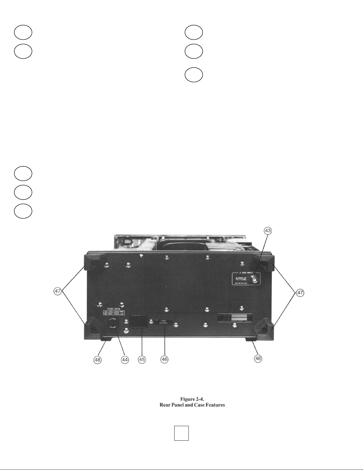
2-1-4 Miscellaneous

Refer to Figure 2-4 for references (43) to (48).

Z AXIS INPUT For applying signal to intensity Connector modulate the CRT.

FUSE Receptacle permits quick fuse re-

placement without opening case

Power Connector Permits removal or replacement of AC

power cord.

Voltage Label Indicates the voltage of the oscil-

loscope's primary wiring.

Cord Caddy Provides a quick method of securing

the power cord, and supports the oscilloscope for vertical operation.

Feet Supports the oscilloscope for shelf

mounting.

2-2. INITIAL OPERATION

Before the instrument is operated for the first time, perform the following procedures in the order listed to ensure satisfaction and prevent damage to the instrument.

2-2-1 Power Connections and Adjustments

The instrument is normally shipped wired for a 120-volt power source but can be adapted to operate from power sources with - 10% of the rated values given in Table 2-1. Operation with a voltage less that t0% of the rated value may result in improper performance of the instrument and a voltage more than 10% in excess of the rated value may damage the power supply circuitry.

To check or alter the power-transformer wiring, proceed as follows:

1. Disconnect the power cord from the Power Connector (45).

2. Remove the 14 Phillips-head screws around the periphery of the

top and bottom covers.

3. Remove the covers and carefully turn the LBO-516 upside

down.

Page 11

4. Compare the wiring of the power transformer to that shown in Figure 2-5. If you want to adapt the instrument to operate from a different voltage, determine the correct wiring diagram from Table 2-1.

5. Unsolder any connections not appropriate to the desired connection, and install the new wiring.

6. Change the fuse (if necessary) to the value indicated in Table 21 for the selected voltage range. In all cases the fuse must be the delayed-action ("SLO-BLOW') type.

Table 2-1

POWER TRANSFORMER PRIMARY WIRING

Nominal Voltage 100V 120V 200 V 220 V 240 V

2-2-2 Installation

The LBO-516 will operate in either a horizontal or vertical

position, so it is highly suited to field or laboratory work. It can therefore be positioned on a bench top, riser shelf, or even the floor.

Voltage Range 90-110V 110-130 V 180-220 V 200-240 V 215-265 V

Rating Wiring

Diagram

1.25 A

0.80 A

B C D E F

For bench-top mounting, it is advantageous to have the front of the instrument tilted upward for straight-on viewing. Press in the two Handle-position Locks and simultaneously rotate the Handle so it points below the case, then release the locks.

If the instrument is placed on a riser shelf above the work bench, rotate the Handle above the instrument and as far towards the back as possible. It is not necessary to lock it in this position.

If lack of working space requires that the instrument be placed on the floor, stand the LBO-516 on end. The Cord Caddy (47) will act as legs to support the instrument. Rotate the Handle just enough back for clear access to the front-panel controls.

The LBO-516 is designed to operate over a temperature range of 0°C to +40°C (32°F to 104°F) and a humidity range of 10 to 90%. Operation in a more severe environment may shorten the life of the instrument.

Operation in a powerful magnetic field may distort the waveform or tilt the trace. This is most likely to occur if the instrument is operated close to equipment having large motors or power transformers.

2-2-3 Preliminary Control Settings and Adjustments

1. Set the following controls as indicated:

AC/GND/DC switches (16) ........... AC

Page 12

VOLTS/DIV switches (10) ............. 2V

VARIABLE VOLTS/DIV controls (11) Fully CW, and

pushed in

V MODE switches (21) ................ ALT

Vertical POSITION controls (17 & 18) Index up

A INTEN control (3) ................... Index up

FOCUS control (5) ..................... Index up

ILLUM control (8) ...................... Fully CCW

CH-2 INV switch (19) ................. Out

PULL TRIPLE control (22) ........... Pushed in

PULL QUAD control (23) ............. Pushed in

HORIZ DISPLAY switches (31) ..... A

B TIME/DIV switch (25) .............. Any Ps

A TIME/DIV switch (24) .............. .2 mS

A VARIABLE control (26)

Horizontal POSITION control (29) .. Index up

SOURCE switch (34) .................. CH-1

COUPLING switch (36) ............... AC

SWEEP MODE switches (37) ....... AUTO.

HOLDOFF control (42) ................ Fully CCW, and

2. Plug the power cord into a convenient AC receptacle and press in the POWER switch (1). Shortly, two traces should appear. If the traces appear extremely bright, turn the A INTEN control (3) counterclockwise. Otherwise, let the instrument warm up for a few minutes.

CAUTION:

in the CRT. However, if the CRT is left with an extremely bright dot or trace for a very long time, the fluorescent screen may be damaged. Therefore, if a measurement requires high brightness, be certain to turn down the INTEN control immediately afterward. Also, get in the habit of turning the brightness way down if the scope is left unattended for any period of time.

3. Turn the A INTEN control (3) to adjust the brightness to the desired amount.

4. Turn the FOCUS control (5) for a sharp trace.

5. Turn the CH-1 vertical POSITION control (17) to move the CH1 trace two divisions down from the top of the graticule grid. Turn the CH-2 vertical POSITION control (18) to move the CH2 trace two divisions up from the bottom of the graticule grid.

6. See if the traces are precisely parallel with the graticule lines. If they are not, adjust the ROTATION control (6) with a small screwdriver.

7. Turn the horizontal POSITION control (29) to align the left edge of the traces with the left-most graticule line.

8. Connect the CH- 1 (14) and CH-2 (15) input connectors to the CAL connector (9). The TRIG'D lamp (41) should light and two rectangular waveforms appear on the CRT screen.

9. Carefully examine the waveform, particularly at the corners, while adjusting the FOCUS control to assure sharpest focus.

10. Disconnect the vertical inputs from the calibrator.

...........

A burn-resistant fluorescent material is used

Fully CW, and

pushed in

pulled out

2-3 BASIC OPERATING PROCEDURES

The following paragraphs in this section describe how to operate the LBO-516, beginning with the most elementary operating modes, and progressing to the less frequently-used and/or complex modes.

2-3-1 Signal Connections

There are three methods of connecting an oscilloscope to the signal you wish to observe. They are: a simple wire lead, coaxial cable, and scope probes.

A simple lead wire may be sufficient when the signal level is high and the source impedance low (such as TTL circuitry), but is not often used. Unshielded wire picks up hum and noise; this distorts the observed signal when the signal level is low. Also, there is the problem of making secure mechanical connection to the input connectors. A binding post-to-BNC adapter is advisable in this case.

Coaxial cable is the most common method of connecting an oscilloscope to signal sources and equipment having output connectors. The outer conductor of the cable shields the central signal conductor from hum and noise pickup. These cables are usually fitted with BNC connectors on each end, and specialized cables and adaptors are readily available for mating with other kinds of connectors.

Scope probes are the most common method of connecting the oscilloscope to circuitry. These probes are available with 1X attenuation (direct connection), 10X and 100X attenuation. The 10X attenuator probe increases the effective input impedance of the probe/scope combination to 10 megohms shunted by a few picofarads. The 100X probe increases the effective input impedance of the probe/scope combination to anywhere from 10 to 100 megohms shunted by a few picofarads, depending upon probe model. The reduction in input capacitance is the most important reason for using attenuator probes at high frequencies, where capacitance is the major factor in loading down a circuit and distorting the signal.

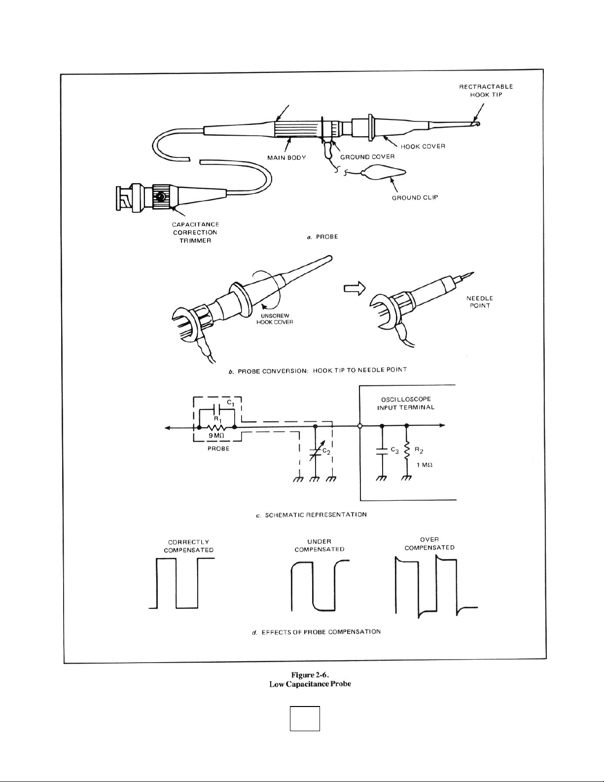
Despite their high input impedance, attenuator probes do not pick up appreciable hum or noise. As was the case with coaxial cable, the outer conductor of the probe cable shields the central signal conductor. Scope probes, of any attenuation, are also quite convenient from a mechanical standpoint. Nearly all quality probes have a spring-loaded hook end that quickly and securely holds the probe to wiring and component leads (see Figure 2-6). This hook can be removed to expose a needlepoint, excellent for use on the foil side of a pc board, or for quickly moving from one point to another.

To determine if a direct connection with shielded cable is permissible, you must know the source impedance of the circuit you are connecting to, the highest frequencies involved, and the capacitance of the cable. If any of these factors are unknown, use a 10X low-capacitance probe.

An alternative connection method at high frequencies is terminated coaxial cable. A feed-thru terminator having an impedance equal to that of the signal-source impedance, is connected to the input connector of the oscilloscope. A coaxial cable of matching characteristic impedance connects the signal source to the terminator. This technique allows using cables of nearly any practical length without signal loss.

9 10

Page 13

Page 14

If a low-resistance ground connection between oscilloscope and circuit is not established, enormous amounts of hum will appear in the displayed signal. Generally, the outer conductor of shielded cable provides the ground connection. If you are using plain lead wire, be certain to first connect a ground wire between the LBO-516 Ground connector (12) and the chassis or ground bus of the circuit under observation.

WARNING:

chassis (via the 3-prong power cord). Be certain the device to which you connect the scope is transformer operated. Do NOT connect the LBO-516 or any other test equipment to "AC/ DC", "hot chassis", or "transformerless" devices. Similarly, do NOT connect the LBO-516 directly to the AC power line or any circuitry connected directly to the power line. Damage to the instrument and severe injury to the operator may result from failure to heed this warning.

2-3-2 Single-trace Operation

Single trace operation with single timebase and internal triggering is the most elementary operating mode of the LBO-516. Use this mode when you want to observe only a single signal, and not be disturbed by other traces on the CRT. Since the LBO-516 is fundamentally a two-channel instrument, you have a choice for your single channel. Channel 1 has an output terminal; use channel 1 if you also want to measure frequency with a counter while observing the waveform. Channel 2 has a polarity-inverting switch. While this adds flexibility, it is not ordinarily used in single-trace operation.

The LBO-516 is set up for single-trace operation as follows:

1. Set the following controls as indicated. Any controls not

mentioned here or in the following steps can be

neglected. Note that the trigger source selected (CH-1 or

CH-2 SOURCE) must match the single channel selected

(CH-1 or CH-2 V MODE).

VARIABLE VOLTS/DIV Fully CW,

controls (11) and pushed in

AC/GND/DC switches (16) .......... AC

V MODE switches (21) ............... CH- 1 or CH-2*

CH-2 INV switch (19) .................. Out

A INTEN control (3) ................... APS**

FOCUS control (5) ..................... APS**

POWER switch (1) ..................... In

HORIZ DISPLAY switches (31) ..... A

B TIME/DIV switch (25) .............. 0.5/KS

A VARIABLE control (26) ............ Fully CW, and

SOURCE switch (34) .................. CH- 1 or CH-2*

COUPLING switch (36) ............... AC

SWEEP MODE switches (37) ........ AUTO

HOLDOFF control (42) ................ Pulled out

Horizontal POSITION control (29) ..APS**

*These selections must match.

**As previously set.

2. Use the corresponding vertical POSITION control (17)

or (18) to set the trace near mid screen.

The LBO-516 has an earth-grounded

pushed in

PRESET level

3. Connect the signal to be observed to the corresponding input connector (14) or (15), and adjust the corresponding VOLTS/DIV switch (10) so the displayed signal is totally on screen.

CAUTION:

4. Set the A TIME/DIV switch (24) so the desired number of cycles of signal are displayed. For some measurements just 2 or 3 cycles are best; for other measurements 50-100 cycles (appears like a solid band) works best.

5. If the signal you wish to observe is so weak that even the 5 mV position of the VOLTS/DIV switch cannot produce sufficient trace height for triggering or a usable display, pull the VARIABLE (X10 MAG) control (11) outwards. This produces 1 mV/div sensitivity when the VOLTS/DIV switch is set to 10 mV, and .5 mW/div when it is set to 5 mV.

6. If the signal you wish to observe is so high in frequency that even the .02/KS position of the A TIME/DIV switch

results in too many cycles displayed, pull the A VARIABLE (X10 MAG) control (28) outwards. This increases the effective sweep speed by a factor of 10, so .02 KS/div becomes 2KS/div, .1/KS becomes .01 KS/div, etc. The 2KS/div sweep speed achievable by magnification is fast enough to display a single cycle of a 50 MHz signal across the CRT face!

7. If the signal you wish to observe is either DC or low enough in frequency that AC coupling attenuates or distorts the signal, flip the AC/GND/DC switch (16) to DC.

CAUTION:

2-3-3 Triggering Alternatives

Triggering is often the most difficult operation to

perform on an oscilloscope because of the many options available and the exacting requirements of certain signals. By using PRESET trigger level and the AUTO sweep mode, error-free triggering is obtainable from the LBO-516. These were the trigger options selected for the single-trace operating procedure described in paragraph 2-3-2, and the multi-trace and dual-time base operating modes described in the following section. They will in fact work well with most signals. However, for complex or otherwise difficult signals, the LBO-516 operator may choose from an extensive selection of trigger options. These are categorized as triggersource options, coupling options, sweep mode, and triggerpoint selection.

Sweep Mode Selection. Normally, the CRT beam is not

swept horizontally across the face of the CRT until a sample of the signal being observed, or another signal harmonically related to it, triggers the timebase. This is the situation when NORM SWEEP MODE (37) is selected. However, this trigger mode is inconvenient because no baseline appears on the CRT screen in the absence of an input signal, or if the trigger controls are improperly set. Since an absence of a trace can also be due to an improperly set vertical position control or VOLTS/DIV switch, much time can be wasted determining the cause. The AUTO sweep mode solves this problem by causing the timebase to automatically free run when not triggered. This yields a single horizontal line with no signal,

greater than 400 V (DC + AC peak).

If the observed waveform is low-level AC, make certain it is not riding on a highamplitude DC voltage.

Do not apply a signal

Page 15

and a vertically-deflected but non-synchronized display when vertical signal is present but the trigger controls improperly set. This immediately indicates what is wrong. The only problems with AUTO operation are that signals below 20 Hz cannot, and complex signals of any frequency may · not, reliably trigger the timebase. Therefore, the usual practice is to leave the AUTO pushbutton pushed in, but press NORM if any signal (particularly one below 20 Hz) fails to produce a stable display.

The third sweep mode, obtained by pressing the SINGLE pushbutton, produces a nonrepetitive sweep. Its use is described in

Trigger Source Options.

obtained from the signal applied to the vertical inputs, or from a separate source of the same or a harmonically-related frequency. The SOURCE switch (34) offers several choices.

The CH-1 and CH-2 positions offer a choice of which of the two input channels the trigger signal is derived. The choice of channels remains even if the trigger channel is not displayed; the only requirements are that signal be applied to the trigger-source channel and the associated VOLTS/DIV switch be set to provide sufficient signal amplitude. The minimum trigger amplitude is around half a division below 10 MHz, and increases to 1 1/2 divisions at 100 MHz. For insurance, use at least a full division below 10 MHz, and two divisions above 10 MHz.

If both channels are displayed, and the two signals are different but harmonically-related frequencies, trigger from the low-frequency channel if possible. This will ensure that traces are stable.

Select the ALT position when you want to display two signals not harmonically related (720 Hz and 939 Hz, for example). The ALT SOURCE position must be used in conjunction with the ALT V MODE (21) pushbutton for this type of dual-trace display.

The LINE position provides trigger signal at the local power-line frequency. This is of great use when you wish to observe a low-level ripple component imposed on a large DC voltage, or within a mixture of other AC voltages. The linefrequency trigger will sync signal at any reasonable multiple of the power-line frequency.

2-3-10 Single-shot Operation.

Trigger signal can be

The 0.2 V/DIV and 2 V/DIV positions both select external trigger signal applied to the EXT TRIG IN connector (35). Use 0.2 V/DIV position when the external trigger amplitude is between 100 mV and 2000 mV peak-topeak. Use the 2 V/ DIV position when the signal amplitude is between 2 V and 20 V peak-to-peak.

CAUTION:

V (DC + AC peak).

Using a trigger source not derived from the channel you are watching has the advantage that changes in the amplitude of the signal under observation will not cause the display to lose sync, even if the amplitude of the observed signal falls below a half graticule division. External trigger also has the advantage that complex and/or noisy signals can be stably displayed, providing the trigger signal is free of noise.

Trigger Coupling Options.

coupling options for the main (A) and delayed (B) timebases increase the probability of stable triggering on difficult signals, such as those containing several frequencies and/or hum and noise.

The first two COUPLING positions (36) are frequencyselective filters that pass certain frequencies on to the trigger circuitry and reject others. The AC position removes any DC component in the trigger signal.

The HF-REJ position cuts off frequencies higher than 35 kHz, passing only signals in the 10 Hz to 35 kHz region. Select this position if high-frequency noise (the CHOP switching pulses for example) is mixed with a low-frequency signal.

The DC position removes all filters from the trigger chain, so everything in the trigger signal from DC to the upper bandwidth limit of the oscilloscope is passed to the trigger circuits. Select DC COUPLING if the trigger signal is below 10 Hz, or may be expected to be below this frequency at some time during a series of measurements.

The TV-V and TV-H positions insert a TV sync separator into the trigger chain, so a clean trigger signal at either the vertical or horizontal repetition rates can be removed from a composite video signal. The TV-V position is also effective in securing stable triggering at the low frequency (60 or 70 Hz) of an audio intermodulation distortion

Do not apply a signal greater than 400

The various trigger

Page 16

test signal. To trigger the scope at the vertical (field) rate, select the TV-V position. To trigger the scope at the horizontal (line) rate, select the TV-H position. When either TV position is used, the SLOPE switch (39) must be matched to the polarity of the video signal. Leave the SLOPE pushbutton out (+ position) for positive-sync signals (Figure 2-7a), and push it in (- position) for negative-sync video signals (Figure 2-7b).

timebase must be triggered at the exact same point on the re-

Trigger Point Selection

current waveform each time the timebase is swept. This is sometimes difficult to achieve, so the LBO-516 has three controls that enable the operator to achieve this condition. They are the LEVEL control (40), the SLOPE switch (39), and the HOLDOFF control (42).

. For a stable display, the

The SLOPE switch determines whether the sweep will begin on a positive-going or negative-going slope of the trigger signal (see Figure 2-8). In some cases, the choice of slope is unimportant; in others, it is vitally important to attain a stable and/or jitter-free display. Always select the steepest and most stable slope or edge. For example, small changes in the amplitude of the sawtooth shown in Figure 2.8a will cause jitter if the timebase is triggered on the positive (ramp) slope, but have no effect if triggering occurs on the negative slope (a fast-fall edge). In the example shown in Figure 2-8b, both leading and trailing edges are very steep (fast rise and fall times). However, this particular pulse is the output of a leading-edge triggered monostable, and has pulse-width jitter. Triggering from the jittering trailing edge will cause the entire trace to jitter, making observation diffi-

Page 17

cult. Triggering from the stable leading edge (+ slope) yields a trace that has only the trailing-edge jitter of the original signal. If you are ever in doubt, or have an unsatisfactory display, try both slopes to find the best way.

The LEVEL control determines the point on the selected slope at which the main (A) timebase or delayed (B) timebase will be triggered. The effect of the LEVEL control on the displayed trace is shown in Figure 2-9a. The +, 0, and - panel markings for this control refer to the waveform's zero crossing and points more positive (+) and more negative (-) than this. If the trigger slope is very steep, as with square waves or digital pulses, there will be no apparent change in the displayed trace until the LEVEL control is rotated past the most positive or most negative trigger point, whereupon the display will free run (AUTO sweep mode) or disappear completely (NORM sweep mode). Try to trigger at the mid point of slow-rise waveforms (such as sine and triangular waveforms), since these are usually the cleanest spots on such waveforms. As figure 2-9b shows, triggering on a noisy area will cause instability in the display. Pulling the HOLDOFF control outwards to the PRESET level position automatically triggers the timebase near the zero-crossing point of the trigger signal.

The larger the amplitude of the trigger signal inputted to the trigger circuits, the greater is the degree of rotation (control range) over which the LEVEL control will maintain a stable display. With internally-derived trigger, the actual trigger amplitude is proportional to the number of graticule divisions occupied by the trace. Therefore, the trigger point is more critical with small signals than large. This is one reason why it is important to use as much trace height as practical for the number of traces displayed.

The HOLDOFF control is used for special circumstances only. It allows the operator to alter the mandatory "dead" time between the end of one sweep and the start of the next (in response to a trigger pulse). This prevents the triggering of subsequent sweeps by the wrong trigger pulse in a complex waveform. During normal operation, leave the HOLDOFF control click-stopped at NORM. When viewing complex waveforms containing multiple trigger points per repetition, rotate the HOLDOFF control clockwise until the proper waveform is secured, as shown in Figure 2-10. For example, the waveform shown contains three pulses in each group capable of triggering the timebase, but sweep must begin only on the first pulse in each burst to obtain the proper display. In the lower display, the dead time has been extended enough to make it impossible for last pulse in the second burst to start the next sweep.

Rotate the HOLDOFF control fully clockwise to its B ENDS A click-stopped position when using the delayed (B) timebase and the difference between the A and B TIME/DIV setting is large (6 positions or more). The resulting brightness improvement is greatest when the delay time between B and A timebases is short.

2-3-4 Probe Compensation

The LP- 100X probes furnished with the LBO-516 must be adjusted to the input capacitance of the. channel(s) with which they are used. If the probes are used only with vertical input channels 1 and 2, this adjustment need be performed only when the probes are first used, and the probes can be used interchangeably between these channels without adjustment. However, if an additional probe is purchased for the trigger input channel (CH-3), mark it and compensate it separately, as the CH-3 input capacitance is somewhat different.

To compensate a probe for CH-1 or CH-2, proceed as follows:

1. Connect the probe to the CH-1 input connector (14) and the

CAL connector (9).

2. Set the CH- 1 VOLTS/DIV switch (10) to 20 mV, the CH- 1

AC/GND/DC switch (16) to DC, and the A TIME/DIV

switch (24) to .2 mS.

3. Press the CH-1 V MODE pushbutton (21) and A HORIZ

DISPLAY pushbutton (35), and select CH-1 SOURCE (34).

4. With a small screwdriver, adjust the capacitance-correction

trimmer (Figure 2-6a) for a correct-appearing square wave.

(Figure 2-6d).

Page 18

To compensate a probe for CH-3, proceed as follows:

1. Connect the probe to the CH-3 or EXT TRIG IN connector (35) and a 1000 Hz signal source set for 8 Vp.p output amplitude.

2. Set the A TIME/DIV switch to .2 mS, the SOURCE switch to .2 V/DIV, and the COUPLING switch to DC.

3. Press the ALT V MODE pushbutton (21), the A HORIZ DISPLAY pushbutton (35), and push in the HOLDOFF control (42).

4. Pull the PULL TRIPLE control (22) and adjust it to position the CH-3 trace at midscreen. Adjust the LEVEL control (40) if needed.

5. With a small screwdriver, adjust the capacitance-correction trimmer (Figure 2-6a) for a correct-appearing square wave. (Figure 2-6d).

2-3-5 Dual Trace Operation

Dual-trace operation is the major operating mode of the

LBO-516, since full amplification and attenuation facilities are provided for the two channels. As was the case with Single-trace Operation, you have a choice here too, not of channel selection, but of how to display the two channels.

The LBO-516 is set up for dual-trace operation as follows:

1. Set the following controls as indicated below. Any controls not

mentioned here or in the following steps can be neglected.

VARIABLE VOLTS/DIV controls (11) Fully CW, and

pushed in

AC/GND/DC switches (16) ......................... AC

CH-2 INV switch (19) ................................. Out

PULL TRIPLE control (22) ......................... In

PULL QUAD control (23) ........................... In

A INTEN control (3) ................................... APS*

FOCUS control (5) ...................................... APS*

POWER switch (1) ..................... In

HORIZ DISPLAY switches (31) ..... A

B TIME/DIV switch (25) .............. 0.5/PS

A VARIABLE control (26) ........... Fully CW, and

pushed in.

SOURCE switch (34) .................. CH-I or CH-2**

COUPLING switch (36) ............... AC

SWEEP MODE switches (37) ........ AUTO

HOLDOFF control (42) ............................... Pulled out

.................................................................... (PRESET level)

Horizontal POSITION control (29) .............. APS*

*As previously set. **See Step 6.

Page 19

2. Press either ALT or CHOP V MODE pushbutton (21). Press ALT for relatively high-frequency displays (A TIME/DIV switch set at .2 mS or faster); press CHOP for relatively lowfrequency displays (A TIME/DIV switch set at .5 mS or slower). If the CHOP pushbutton is pressed when fast sweep speeds are used, the displayed traces will appear broken (as in Figure 2-11) when signals are applied. If the ALT pushbutton is pressed when slow sweep speeds are used, the display will flicker excessively.

3. Use the vertical POSITION controls (17 and 18) to set the CH-1 trace about two divisions down from the top graticule line, and the CH-2 trace about two divisions up from the bottom graticule line.

The LBO-516 is set up for dual-trace operation as follows:

4. Connect the signals to be observed to the CH-1 and CH-2 IN connectors (14) and (15), and adjust the VOLTS/DIV switches (10) so the displayed signals are totally on screen and clear of each other.

CAUTION:

(DC + AC peak).

5. Set the A TIME/DIV switch (24) so the desired number of cycles are displayed. Be certain the display mode (ALT or CHOP) selected is consistent with this sweep speed (as per Step 2).

6. If both channels are handling signals of the same frequency, trigger from the channel having the steepest-slope waveform. If the signals are different but harmonically-related frequencies, trigger from the channel carrying the lowest frequency. Also, bear in mind that if you disconnect the signal to the channel serving as the trigger source, the entire display will free run.

7. If the signals are different frequencies and not harmonically related, select the ALT trigger SOURCE position (34) and the ALT V MODE pushbutton (21) regardless of the A TIME/DIV switch setting.

8. If the signal you wish to observe is so weak that even the 5 mV position of the VOLTS/DIV switch cannot produce sufficient trace height for triggering a usable display, pull the VARIABLE (XI0 MAG) control (11) outward. This produces 1 mV/ div sensitivity when the VOLTS/DIV switch is set to I0 mV, and .5 mV/div when it is set to 5 mV.

Do not apply signals greater than 400 V

9. If the signal you wish to observe is so high in frequency that even the .02/aS position of the A TIME/DIV switch results in too many cycles displayed. Pull the A VARIABLE (XI0 MAG) control (26) outward. This increases the effective sweep by a factor of 10, so .02 PS/div becomes 2 KS/div,

0.1PS/div becomes .01 /PS/div, etc. The 2 KS/div sweep speed achievable by magnification is fast enough to display a single cycle of a 50 MHz signal across the CRT face.

10. If the signal you wish to observe is either DC or low enough in frequency that AC coupling attenuates or distorts the signal, flip the AC/GND/DC switch (16) to DC.

CAUTION:

low-level AC, make certain it is not riding

2-3-6 Additive and Differential Operation

Additive and differential operation are forms of two-channel

operation where two signals are combined to display one trace. In additive operation, the resultant trace represents the algebraic sum of the CH-1 and CH-2 signals. In differential operation, the resultant trace represents the algebraic CH-I and CH-2 signals.

To set up the LBO-516 for additive operation, proceed as

follows:

1. Set up the dual-trace operation per paragraph 2-3-5, Steps 1 to 6 and 8 to I0.

2. Make sure both VOLTS/DIV switches (I0) are set to the same position; and the VARIABLE controls (11) are detented in their CAL'D position. If the signal levels are very different, set both VOLTS/DIV switches to the position producing a large on-screen display of the

signal.

3. Trigger from the channel having the biggest signal.

4. Press the ADD V MODE (21) pushbutton. The single trace resulting is the algebraic sum of the CH- 1 and CH-2 signals. Either or both of the vertical POSITION controls (17) and (18) can he used to shift the resultant trace.

5. If the p-p amplitude of the resultant trace is very small, mm

both

Make sure both VOLTS/DIV controls are set to the same position. To set up the LBO-516 for differential operation, proceed as

follows:

1. Set up for dual-trace operation per paragraph 2-3-5,

2. Ensure that both VOLTS/DIV switches (10) are set to

3. Trigger from channel having the larger signal.

4. Press in the CH-2 INV pushbutton (19).

on a high-amplitude DC voltage.

NOTE: If the input signals are in-phase, the amplitude of the resultant trace will be the arithmetic sum of the individual traces (e.g., 4.2 div + 1.2 div = 5.4 div). If the

input signals are 180° out of phase, the amplitude of the resultant trace will be the arithmetic difference of the two traces (e.g., 4.2 div - 1.2 div = 3.0 div).

VOLTS/DIV switches to increase the display height.

Steps 1 to 6 and 8 to I0.

the same position. If the signal levels are very different, temporarily set both VOLTS/DIV switches to the position needed to produce a large on-screen display of the highest-amplitude signal.

If the observed waveform is

difference

between the

higher amplitude

Page 20

5. Press the ADD V MODE pushbutton (21)· The single trace resulting is the algebraic difference of the CH-1 and CH-2 signals. Either or both of the vertical POSITION controls (17) and (18) can be used to shift the resultant trace.

NOTE: If the input signals are in-phase, the amplitude of the resultant trace will be the arithmetic difference of the individual traces (e.g., 4.2div - 1.2div = 3.0div). If

the input signals are 180° out of phase, the amplitude of the resultant trace will be the arithmetic sum of the individual traces (e.g., 4.2 div + 1.2 div = 5.4 div).

6. If the peak-to-peak amplitude of the resultant trace is very small, mm both VOLTS/DIV switches to increase the display height. Make sure both VOLTS/DIV controls are set to the same position.

2-3-7 Triple-trace Operation

A very useful feature of the LBO-516 is that the timebase

trigger can be displayed on the CRT screen along with the two vertical inputs. The trigger signal appears as the third trace, permitting continuous trigger view and/or a third input channel.

Trigger Display.

trigger signal and two input channels, proceed as follows:

1. Set the following controls as indicated below. Any

controls not mentioned here or in the following steps can be neglected.

PULL TRIPLE control (22) ......................... Pulled out

CH-2 INV switch (19) ................................. Out

VARIABLE VOLTS/DIV Fully CW, and

controls (11) pushed in

AC/GND/DC switches (16) .......................... AC

PULL QUAD control (23) ........................... Pushed in

A INTEN control (3) ................................... APS*

FOCUS control (5) ...................................... APS*

POWER switch (1) ...................................... Pushed in

HORIZ DISPLAY switches (31) .................. A

B TIME/DIV switch (25) ............................. 05/PS

A VARIABLE control (26) ......................... Fully CW, and

.. ........ ........ ........ ........ ........ ........ ........ ........ .. pushed in

SOURCE switch (34)................................... CH-1 or

.. ........ ........ ........ ........ ........ ........ ........ ........ .. CH-2**

COUPLING switch (36) .............................. AC

SWEEP MODE switches (3'7) ..................... AUTO

HOLDOFF control (42) ............................... Pulled out

.. ........ ........ ........ ........ ........ ........ ........ ........ .. (PRESET level)

Horizontal POSITION control (29) .............. APS*

* As previously set. ** See Step 7.

2. Press the ALT or CHOP V MODE pushbutton (21). Press ALT for relatively high-frequency displays (A TIME/DIV switch set at .2 mS/div and faster); press CHOP for relatively low-frequency displays (A TIME/DIV switch set at .5mS/div and slower). If the CHOP pushbutton is pressed when fast sweep speeds are used, the displayed traces will appear as broken lines when signal is applied. Conversely, if the ALT pushbutton is pressed when low sweep speeds are used, the display will flicker excessively.

To continuously display the timebase

3. Use the vertical POSITION controls (17 and 18) to set the CH- 1 trace near the 90% dotted graticule line, and the CH-2 trace on the center graticule line.

4. Use the PULL TRIPLE control (22) to set the third trace near the 10% dotted graticule line.

5. Connect the signal to be observed to the CH-1 and CH-2 IN connectors (14 and 15), and adjust the VOLTS/DIV switches (10) so the displayed signals are totally on screen and clear of each other.

6. Set the A TIME/DIV switch (24) so the desired number of cycles is displayed. Be certain the display mode (ALT or CHOP) selected is consistent with this switch setting (per Step 2). If the signal you wish to observe is so high in fre-

quency that even the .02 PS position of the A TIME/DIV switch results in too many cycles displayed, pull the A VARIABLE (XI0 MAG) control (26). This increases the effective sweep speed by a factor of 10, so .02 PS/div becomes 2 KS/div.

7. If CH-1 and CH-2 are both handling signals of the same frequency, trigger from the channel haying the steepest waveform. If the signals are different but harmonically-related frequencies, trigger from the channel carrying the lowest frequency.

8. The third trace is the timebase trigger signal. With trigger taken from either CH- 1 or CH-2, the trigger signal may appear to be the same as one of the vertical channels. However, trigger COUPLING switch positions other than DC insert frequency-selective networks into the CH-3 amplifier, so the third trace may appear different at certain frequencies.

NOTE: If ALT trigger source is selected, the third trace will resemble the CH-1 trace, not the composite trigger

channels, proceed as follows:

2-3-8 Four-trace Operation

displayed as the fourth trace in this mode of operation. To display the CH-1 and CH-2 input signals, their algebraic sum, and the signal triggering the timebase, proceed as follows:

signal.

Three Input Channels

1. Perform Steps 1 to 6 of the previous procedure.

2. Connect the third signal to be observed to the EXT

TRIG IN (CH-3) connector (35). If the three signals are different but harmonically-related frequencies, apply the lowest-frequency signal to this channel. CAUTION: Do not apply a signal greater than 400 V (DC + AC peak).

3. Set the SOURCE switch (34) to the 2 V/DIV position. If

the trace is less than one division high, external amplification will be needed.

4. The third trace is the CH-3 input signal as well as the

timebase trigger, so do not use any trigger coupling position other than AC or DC. The bandwidth-limiting filters inserted at other positions of the COUPLING switch (36) will distort the CRT display of the CH-3 input signal.

The algebraic sum of the CH-I and CH-2 input signals is

. To display three independent input

Page 21

1. Set the following controls as indicated. Any control not mentioned here or in the following steps can be neglected.

PULL QUAD control (23) ........................... Pulled out

CH-2 INV switch (19) ................................. Out

VARIABLE VOLTS/DIV controls (11) Fully CW, and

pushed in

AC/GND/DC switches (16) ......................... AC

A INTEN control (3) ................................... APS*

FOCUS control (5) ...................................... APS*

POWER switch (1) ...................................... Pushed in

B TIME/DIV switch (25) .............. . 05P S

HORIZ DISPLAY switches (31) ..... A

A VARIABLE control (26) ........... Fully CW, and

pushed in

SOURCE switch (34) .................. CH-1 or CH-2**

COUPLING switch (36) ............... AC

SWEEP MODE switches (37) ........ AUTO

HOLDOFF control (42) ................ Pulled out

(PRESET level) Horizontal POSITION control (29) .. APS* * As previously set. ** See Step 6.

2. Press the ALT or CHOP V MODE pushbutton (21). Press

ALT for relatively high-frequency displays (A TIME/ DIV switch set at .2 mS/div and faster); press CHOP for relatively low-frequency displays (A TIME/DIV switch set at .5mS/div and slower). If the CHOP pushbutton is pressed when fast sweep speeds are used, the displayed traces will appear as broken lines when signal is applied. Conversely, if the ALT pushbutton is pressed when low sweep speeds are used, the display will flicker excessively.

3. Use the vertical POSITION controls (17 and 18) to set the

CH-1 trace two graticule divisions from the bottom of the CRT screen. This will set the sum trace (CH- 1 + CH-2) near the center graticule line.

NOTE: The position of the sum trace is not separately controllable.

4. Use the PULL TRIPLE control (22) to temporarily set the CH-3 trace off screen.

5. Connect the signals to be observed to the CH-1 and CH-2 IN

connectors (14 and 15), and adjust the VOLTS/DIV switches (10) so the displayed traces are totally on screen and well clear of each other. Make sure both VOLTS/ DIV switches are set to the same position, and their VARIABLE controls (11) are detented in their CAL'D positions. If the signal levels are very different, set both VOLTS/DIV switches to the position suitable for the higher-level signal.

6. Set the trigger SOURCE switch (34) to match the channel

with the higher-amplitude signal.

7. Set the A TIME/DIV switch (24) so the desired number of

cycles is displayed. Be certain the display mode (ALT or CHOP) selected is consistent with this switch setting (per Step 2). If the signal you wish to observe is so high in frequency that even the .02 p3 position of the A TIME/ DIV switch results in too many cycles displayed, pull the A VARIABLE (XI0 MAG) control (26). This increases the

effective sweep speed by a factor of I0, so .02PS/div becomes 2 KS/div.

8. The CH-2 INV switch (19) can be pushed in to display the difference signal between the CH-1 and CH-2 input signals instead of their sum.

9. If your primary reason for selecting the four-trace display mode is to view the sum or difference signal while simultaneously viewing the two signals from which it is derived, leave the CH-3 trace off screen. If you need to see the timebase trigger trace as well, use the PULL TRIPLE control to move the CH-3 trace to a relatively vacant spot on screen.

10. If the CH-3 trace is used as a third input channel, set the trigger SOURCE switch to 0.2 V/DIV or 2 V/DIV, as befits the input-signal amplitude. Since this trace is also the timebase trigger signal, some positions of the trigger COUPLING switch (36) will distort the trace because of the limited-bandwidth filters they insert. Therefore, use either the DC or AC COUPLING settings in this application.

2-3-9 Delayed-timebase Operation

The LBO-516 contains two timebases, arranged so one (the

A timebase) may provide a delay between a trigger event and the beginning of sweep by the second (B) timebase. This allows any selected portion of a waveform, or one pulse of a pulse train, to be spread over the entire screen. Moreover, the CRT can be alternately swept by the two timebases, so both the full waveform and the selected portion appear across the full CRT screen width.

The aforementioned dual-timebase displays can be used with

any of the vertical display modes (single trace, dual trace, triple trace, or quad). The procedure is the same regardless of the number of traces displayed.

Basic Delayed Sweep

follows:

1. Set up the LBO-516 as directed for whatever vertical mode

you desire.

2. Make sure the START pushbutton (32) is out.

3. Press the INTEN BY B pushbutton (31). A section of the trace(s) will intensify (brighten). NOTE: The intensified portion will be quite small if there is a large difference between the settings of the A and B TIME/DIV switches. 4. Turn the B TIME/DIV control (25) until the intensified portion of the trace widens to an amount equal to the portion of the trace you wish to magnify (see Figure 2-12b).

5. Turn the DLY TIME MULT control (28) to position the intensification over the portion of the trace you wish to magnify.

6. Press the B HORIZ DISPLAY pushbutton (31). That portion of the trace intensified in Step 5 now appears spread over the full width of the CRT screen. The trace now displayed is being swept by the B timebase (Figure 2-12c).

7. If needed, additional enlargement is possible by palling the A VARIABLE (X10 MAG) control (26) outward.

. For delayed sweep, proceed as

Page 22

B Intensity Adjustment.

relative to A trace brightness as the difference in A and B TIME/DIV switch setting varies. The B INTEN control (4) allows compensatory adjustment for the brightness difference. This control can be rotated clockwise for increased brightness.

The B trace brightness varies

Alternate Sweep Mode.

main (A) and delayed (B) timebase traces for each vertical channel used. The total number of traces is always doubled. Since up to eight traces may appear in the alternate sweep mode, most of the effort in this procedure involves adjusting trace amplitudes and positions to get an understandable display.

To simultaneously display the A and B timebase traces,

proceed as follows:

1. Adjust the vertical VOLTS/DIV control(s) (10) so each trace displayed does not exceed the number of divisions indicated in Table 2-2. This is simply to insure that there is room for all traces when switching to alternate sweep.

2. For the same reason, position the trace(s) so there is room

each

near equal amplitude.

3. Display the B timebase as described in the preceding paragraph,

4. Press the ALT HORIZ DISPLAY pushbutton (31). The B timebase trace(s) will now be displayed below its corresponding A timebase trace(s).

trace currently displayed for an additional trace of

Basic Delayed Sweep.

This sweep mode displays both

5. If necessary, adjust the A/B TRACE SEP control (33) so the B timebase trace(s) do not overlap the A timebase traces. Some adjustments with the vertical POSITION, VOLTS/DIV, and A/B TRACE SEP controls may be necessary if the display is crowded (as in triple-trace and fourtrace operation).

NOTE:

Positioning eight traces can be difficult at first. The suggested layout is to set the CH-1 baseline two graticule divisions down from the top, and the CH-2 baseline two divisions up from the bottom. This puts the sum or difference trace on the center graticule line. For positive-logic signals (TTL, CMOS, etc.), set the CH-3 baseline on the bottom graticule line, and later set the alternate B-sweep display

above

the A-sweep traces. For negative-logic signals (such as ECL), set the CH-3 baseline on the top graticule line, and later set the alternate B-sweep display traces.

6. In measurement situations where the B sweep is very dim (even with the B INTEN control (4) fully clockwise), you can greatly increase the B sweep brightness by rotating the HOLDOFF control (42) clockwise until it clicks into its B ENDS A position. However, this will eliminate the A trace from the intensified position onward. (See Figure 2-13).

below

the A-sweep

Page 23

Triggered B Sweep

is not triggered by a signal event; it begins when the main sweep (A timebase) ends. This is readily seen in the alternate sweep mode. The only problem with this is that main timebase jitter becomes apparent in the B sweep when at high ratios of A to B TIME/DIV switch settings (100:1 and up). To circumvent this, the B sweep can be triggered by the signal itself or a time-related trigger signal. The DLY TIME MULT control then determines the

minimum

time will be that plus the additional time until the next available trigger. The result is that actual delay time is variable only with step resolution, in increments of the interval between triggers.

get-signal supplied to the A timebase. For triggered B sweep, proceed as follows:

1. Set up the scope for basic delayed or alternate sweep as

2. Press in the START pushbutton (32). The B timebase is now

2-3-10 Single-shot Operation

photograph a non-recurrent or transient event. The operation itself is simple, but requires some preparation to ensure its success. To set up for single-shot operation, proceed as follows:

1. Connect the CH-1 IN connector (14) to a signal source (a

2. Adjust the LBO-516 controls for the desired display, pref-

3. Press the NORM SWEEP MODE pushbutton (37), set the

4. Adjust the LEVEL control (40) for a stable trace.

delay time between A and B sweeps; the actual delay

The B timebase is triggered internally, using the same trig-

described in the preceding paragraphs.

triggering on a signal related in time to the A timebase trigger. The start of the B sweep will always be a leading or trailing edge of the trigger signal, turning the DELAY TIME control will not change this.

NOTE:

V, the B timebase trigger signal will be filtered by the TV-H filter. This facilitates inspection of complex signals containing composite sync, such as VITS, VIRS, and various coding signals found in the vertical interval.

Single-shot or single-sweep operation is used to observe or

pulse generator, for example) adjusted to produce recurrent output pulses having the same polarity, amplitude, and pulse width expected of the transient pulse to be observed. Keep the repetition rate low (10 Hz or less) to get an idea of what trace brightness will be like when observing the transient.

erably single-channel. Ensure that the channel 1 trace amplitude is at least 2 divisions.

NOTE:

Multichannel operation is possible, but the CHOP vertical mode must be used regardless of the sweep speed. Because of the dim and broken trace resulting from CHOP operation at high sweep speeds, a single channel is recommended for single-shot observation of fast transients.

COUPLING switch (36) to DC, and the SOURCE switch (34) to CH-1.

. In basic delayed sweep, the B timebase

If the COUPLING SWITCH (36) is set to TV-

5. Disconnect the substitute signal source, then connect the CH- 1 IN connector to the transient to be observed.

6. Press the SINGLE SWEEP MODE pushbutton (37) twice. After the second time, the READY lamp (38) will light.

7. The LBO-516 is now ready to display the transient. When it occurs, the TRIG'D lamp (41) will flash, and the timebase will sweep once, displaying the transient. When the sweep starts, the READY lamp will go out. The sweep cannot be retriggered by another transient until the SINGLE SWEEP MODE pushbutton is pushed again.

2-3-11 X-Y Operation

The internal timebase of the LBO-516 is not utilized in X-Y

operation. Deflection in both the horizontal and vertical directions is via external signals. One of the vertical input channels serves as the X-axis (horizontal) signal processor, so horizontal and vertical axes have identical control facilities.

All of the V MODE, HORIZ DISPLAY, trigger SOURCE

and COUPLING, and SWEEP MODE switches, as well as their associated controls and connectors are inoperative in the X-Y mode.

To set up the LBO-516 for X-Y operation, proceed as fol-

lows:

1. Push in the X-Y pushbutton (20).

CAUTION:

undeflected spot is very bright, or you may damage the CRT phosphor screen

2. Apply the vertical signal to the CH-2 or Y IN connector (15), and the horizontal signal to the CH-1 or X IN connector (14). Once the trace is deflected, adjust the A INTEN control (3) for suitable brightness.

3. Adjust the trace height with the CH-2 VOLTS/DIV switch (10), and the trace width with the CH-1 VOLTS/DIV switch (10). The VARIABLE VOLTS/DIV controls (11) and their associated X10 MAG switches can also be used to adjust trace amplitude along either axis.

4. Adjust the trace position vertically (Y axis) with the CH2 vertical POSITION or Y control (18). Adjust the trace position horizontally (X axis) with the horizontal POSITION control (29) and X FINE control (30); the CH-1 vertical POSITION control has no effect during X-Y operation.

5. The vertical (Y-axis) signal can be inverted via the CH-2 INV pushbutton (19).

2-3-12 Intensity Modulation

Intensity modulation, also known as Z-axis modulation, is a

rarely-used operational mode wherein an external signal controls the brightness of the CRT trace. Its main applications are in video display and time or frequency marking. When so used, it is usually in conjunction with X-Y operation (described in paragraph 2-3-11).

Reduce the trace intensity immediately if the

NOTE:

The X10 MAG switch on the A VARIABLE control is operative, but should not be used. Keep this knob pushed in.

Page 24

To intensity modulate the CRT, simply connect the modulating signal to the Z AXIS INPUT connector (43) on the back panel. The modulating signal must exceed + 2 volts DC to completely blank the trace at any brightness setting. At low brightness levels, blanking may occur at signal voltages as low as

0.5 volt. A blanking signal in the range of + 2 to + 5 volts DC (TTL high) is recommended.

CAUTION: Do not apply a signal greater than 50 V (DC + AC peak).

2-4 MEASUREMENT APPLICATIONS

This section contains instructions for using your LBO-516 for specific measurement procedures. However, this is but a small sampling of the many applications possible for this oscilloscope. These particular applications were selected to demonstrate certain controls and features not fully covered in BASIC OPERATING PROCEDURES, to clarify certain operations by example, or for their importance and universality.

2-4-1 Amplitude Measurement

The modern triggered-sweep oscilloscope has two major measurement functions. The first of these is amplitude. The oscilloscope has an advantage over most other forms of amplitude measurement in that complex as well as simple waveforms can be totally characterized (i.e., complete voltage information is available).

Oscilloscope voltage measurements generally fall into one of two types: peak-to-peak or instantaneous. Peak-to-peak (p-p) measurement simply notes the total amplitude between extremes without regard to polarity reference. Instantaneous voltage measurement indicates the exact voltage from from each and every point on the waveform to a ground reference. When making either type of measurement, ensure that the VARIABLE controls (11) are rotated fully clockwise and de-tented in their CAL'D position.

Peak-to. Peak Voltages

proceed as follows:

1. Set up the LBO-516 for the vertical mode desired per the

instructions in 2-3 BASIC OPERATING PROCEDURES.

. To measure peak-to-peak voltage,

2. Adjust the TIME/DIV switch (24) or (25) for two or three cycles of waveform, and set the VOLTS/DIV switch (10) for the largest possible totally on-screen display.

3. Use the appropriate vertical POSITION control (17) or (18) to position the negative signal peaks on the nearest horizontal graticule line below the signal peaks, per Figure 2-14.

4. Use the horizontal POSITION control (29) to position one of the positive peaks on the central vertical graticule line. This line has additional calibration marks equal to 0.2 major divisions each.

5. Count the number of divisions from the graticule line touching the negative signal peaks to the intersection of the positive signal peak with the central vertical graticule line. Multiply this number by the VOLTS/DIV switch setting to get the peak-to-peak voltage of the waveform. For example, if the VOLTS/DIV switch were set to 2 V, the waveform shown in Figure 2-14 would be 11.2Vp-p (5.6 div X 2V).

6. If X10 vertical magnification is used, divide the Step 5 voltage by 10 to get the correct voltage. If 10X attenuator probes are used, multiply the voltage by 10. However, if X 10 vertical magnification and 10X attenuator probes are used, their effects cancel and the Step 5 voltage can be used without correction.

7. If measuring a sine wave below 100 Hz, or a rectangular wave below 1000 Hz, flip the AC/GND/DC switch to DC.

CAUTION:

a higher-amplitude DC voltage.

Instantaneous Voltages.

proceed as follows:

1. Set up the LBO-516 for the vertical mode desired per the instructions in 2-3 BASIC OPERATING PROCEDURES.

2. Adjust the applicable TIME/DIV switch (24) or (25) for one complete cycle of waveform and set the VOLTS/DIV switch for a trace amplitude of 4 to 6 divisions (see Figure 2-15).

Make certain the waveform is not riding on

To measure instantaneous voltages,

Page 25

3. Position the AC/GND/DC switch (16) to GND.

4. Use the appropriate vertical POSITION control (17) or (18) to set the baseline on the central horizontal graticule line. However, if you know the signal voltage is to be positive,use the 0% or bottom-most graticule line. If you know the signal voltage is to be negative, use the 100% or uppermost graticule line.

NOTE:

The vertical POSITION controls must not be

touched again until the measurement is completed.

5. Position the AC/GND/DC switch to DC. The polarity of all points above the ground-reference line is positive; all points below the ground-reference line are negative.

CAUTION:

on a high-amplitude DC voltage before positioning the AC/GND/DC switch.

6. Use the horizontal POSITION control (29) to position any point of interest on the central vertical graticule line. This line has additional calibration marks equal to 0.2 major divisions each. The voltage relative to ground at any point selected is equal to the number of divisions from that point to the ground reference line multiplied by the

Make certain the waveform is not riding

VOLTS/DIV setting. In the example used for Figure 2-15, the voltage for a 0.5 V/div scale is 2.5 V (5.0 div X 0.5 V).

7. If XI0 vertical magnification is used, divide the Step 6 voltage by 10 to get the correct voltage. If 10X attenuator probes are used, multiply the voltage by 10. However, if X10 vertical magnification and 10X attenuator probes are used, their effects cancel and the Step 6 voltage can be used without correction.

2-4-2 Differential Measurement Techniques

Differential measurement techniques allow direct mea-

surement of the voltage drop across "floating" components (both ends above ground), and measurement of very small signals in electrically noisy environments (such as exist near high-power AC machinery).

The control manipulations for differential operation were

explained in paragraph

Operation.

are shown in Figure 2-16. Figure 2-16a shows the simple technique perfectly satisfactory for measuring high-level signals on floating signals. In this example, the AC voltage drop (ripple) across a power choke is observed

The technique for making the physical connections

2-3-6 Additive and Differential

Page 26

and measured. The ground terminals from the two probes or cables are simply connected to the chassis or ground bus of the circuit under observation. Figure 2-16b shows the connection technique needed for low-level signals in a noisy environment (strong AC fields). Using a separate ground connection and connecting the probe or cable shields to the circuit under test avoids ground loops and EMI pickup. This setup allows fullest utilization of the CMRR (common-mode rejection ratio) of the LBO-516's differential facility.

2-4-3 Time Interval Measurements

The second major measurement function of the triggeredsweep oscilloscope is the measurement of time interval. This is possible because the calibrated timebase results in each division of the CRT screen representing a known time interval.

Basic Technique

interval is described in the following steps. This same technique applies to the more specific procedures and variations that follow.

1. Set up the LBO-516 as described in

Operation.

2. Set the A TIME/DIV switch (24) so that the interval you

wish to measure is totally on screen and as large as possible.

Make certain the A VARIABLE control (26) is rotated fully

clockwise and detented in its CAL'D position. If the UNCAL

lamp (27) is lit, any time interval measurements made under

this position will be inaccurate.

3. Use the vertical POSITION control (17) or (18) to position

the trace so the central horizontal graticule line passes

through the points on the waveform between which you want

to make the measurement.

4. Use the horizontal POSITION controls (29) and (30) to set

the left-most measurement point on a nearby vertical

graticule line.

5. Count the number of horizontal graticule divisions between

the Step 4 graticule line and the second measurement point.

Measure to a tenth of a major division. Note that each minor

division on the central horizontal graticule line is 0.2 major

division.

6. To determine the time interval between the two measurement

points, multiply the number of horizontal divisions counted

in Step 5 by the setting of the A TIME/DIV switch. If the A

VARIABLE control (26) is pulled out (X10 MAG), be

certain to divide the TIME/DIV switch setting by 10.

Period, Pulse Width, and Duty Cycle.

described in the preceding paragraph can be used to determine pulse parameters such as period, pulse width, duty cycle,etc. The period of a pulse or any other waveform is the time it takes for one full cycle of the signal. In Figure 2-17, the distance between points (A) and (C) represent one cycle; the time interval of this distance is the period. The time scale for the CRT display of Figure 2-17a is 10 mS/div, so the period is 70 milliseconds in this example. Pulse width is the distance between points (A) and (B). In our example it is conveniently 1.5 divisions, so the pulse

. The basic technique for measuring time

2-3-2 Single-trace

The basic technique

not

width is 15 milliseconds. However, 1.5 divisions is a rather small distance for accurate measurements, so it is advisable to use a faster sweep speed for this particular measurement. Increasing the sweep speed to 2 mS/div as in Figure 2-17b gives a large display, allowing more accurate measurement. An alternative technique useful for pulses less than a division wide is to pull the A VARIABLE (X10 MAG) control (26) outward, and reposition the pulse on screen with the horizontal POSITION control (29). Pulse width is also called between points (B) and (C) is then called measured in the same manner as pulse width.

When pulse width and period are known, duty cycle can be calculated. Duty cycle is the percentage of the period (or total of on and ofttimes) represented by the pulse width (on time). PW(100) Duty cycle (%) = Period = A

Duty cycle of example = 70 mS = 21.4%

Lead and Lag Time.

quency, but not the same phase, one signal is said to be and the other follows:

1. Set up the LBO-516 as described in

eration

and the other to the CH-2 IN connector (15).

NOTE:

compensated probes, or equal lengths of the same type of coaxial cable to ensure equal delay times.

2. Position the trigger SOURCE selector (34) to the channel

with the leading signal (CH- 1 in the Figure 2-18 example).

3. Use the A TIME/DIV switch (24) to display the time difference as large as possible (Figure 2-18b).

4. Use the CH- l vertical POSITION control (17) to drop the

bottom of the channel 1 trace a little below the central hori-

zontal graticule line, and the CH-2 vertical POSITION

control (18) to raise the top of the channel 2 trace a little

above the line.

5. Use the horizontal POSITION controls (29) and (30) to align

the left-most trace edge (of channel I in this case) with a

nearby vertical graticule line. The horizontal distance

between this line and the point at which the leading edge of

the other trace crosses the central horizontal graticule line

represents the time difference between the two signals. The

channel 1 signal may be said to he leading the channel 2

trace, or the channel 2 trace may be said to be lagging the

channel 1 trace, depending on the point of view.

6. Make sure the A VARIABLE timebase control (26) is ro-

tated fully clockwise and detented in its CAL'D position.

Then, count the number of horizontal divisions between the

leading edges of the traces and multiply this number by the

setting of the A TIME/DIV switch to determine the time

difference. For example, the time difference in Figure 2-18b

is l0 microseconds (5.0 div X 2/PS).

"on"

time in some applications. The distance

off

time. This can be

5mS X 100

When two signals have the same fre-

lagging

. To measure this lead/lag time, proceed as

, connecting one signal to the CH-1 IN connector (14)

At high frequencies use identical and correctly

>>>>

B(100)

>>>>

leading

2-3-5 Dual-trace Op-

Page 27

If the points between which the time difference exists are less than 1 major division apart and located in the middle of complex waveforms that are otherwise in phase, use the delayed (B) timebase as described in select and expand that section of the complex waveform. After doing that, follow the same technique as described in the preceding paragraph. As an alternative, pull the A VARIABLE (X10 MAG) control to expand the traces, and reposition the section with the time difference on screen with the horizontal POSITION controls.

If the points between which the time difference exists are more than 1 but less than 5 major divisions apart, the HighAccuracy Technique described next will yield the greatest accuracy.

High-accuracy Techniques

complex waveform can be measured using the DLY TIME MULT control. The linearity error of this control is only a fraction of a percent, far less than the error possible over a small portion of the timebase sweep.

The delay-time technique can be used with single-trace time measurements (pulse width, period, etc.) or dual-trace measurements (lead and lag time). The technique, after the trace or traces are set up according to the desired procedure, is as follows:

2-3-9 Delayed Timbase Operation

. Closely spaced points within a

1. Set the B TIME/DIV switch (25) to a position 50 to 100 times (5 to 6 positions) faster than the A TIME/DIV switch setting.

2. Press the INTEN BY B HORIZ DISPLAY pushbutton (31), then position the intensified area over the first measurement point by means of the DLY TIME MULT control (28).

3. Press the B HORIZ DISPLAY pushbutton (31) and carefully adjust the DLY TIME MULT control to position the first measurement point exactly over the central vertical graticule line. Record the DLY TIME MULT dial reading.

4. Rotate the DLY TIME MULT control to position the second measurement point over the central vertical graticule line. Record the DLY TIME MULT dial reading.

5. Subtract the Step 3 reading from the Step 4 reading. For example, if the DLY TIME MULT control setting was 4.86 in Step 3, and 7.38 in Step 4, the difference is 2.51.

6. Multiply the Step 5 number by the A TIME/DIV switch setting to find the time difference.

2.4-4 Phase Difference Measurements

Phase difference or phase angle between two signals can be

measured using the dual trace feature of the oscilloscope or by operating the oscilloscope in the X-Y mode. When

Page 28

measuring phase shift of signal-processing devices, the test setup shown in Figure 2-22 can be used.

Dual-trace Method.

waveform (sine, triangle, rectangular, complex pulse, etc.). In fact, it will usually work even if different waveforms are being compared. This method and its variations are effective in measuring small or large differences in phase, at any frequency up to 100 MHz.

To measure phase difference by the dual-trace method,

proceed as follows:

1. Set up the LBO-516 as described in

Operation,

(14) and the other to the CH-2 IN connector (15).

2. Position the trigger SOURCE selector (34) to the channel with the cleanest and most stable trace. Temporarily move the other channel's trace off the screen by means of its vertical POSITION control.

3. Center the stable (trigger source) trace with its vertical POSITION control, and adjust its amplitude to exactly 6 vertical divisions by means of its VOLTS/DIV switch (10) and VARIABLE control (11).

4. Use the LEVEL control (40) to ensure the trace crosses the central horizontal line at or near the beginning of the sweep. (See Figure 2-19.)

5. Use the A TIME/DIV switch (24), A VARIABLE control (26), and the horizontal POSITION control (29) to display one cycle of trace over 7.2 divisions. When this is done, each

major horizontal division represents 50°, and each minor division represents 10

connecting one signal to the CH-1 IN connector

NOTE:

At high frequencies use identical and correctly compensated probes, or equal lengths of the same type of coaxial cable to ensure equal delay times.

This method works with any type of

2-3-5 Dual-trace

°.

Page 29

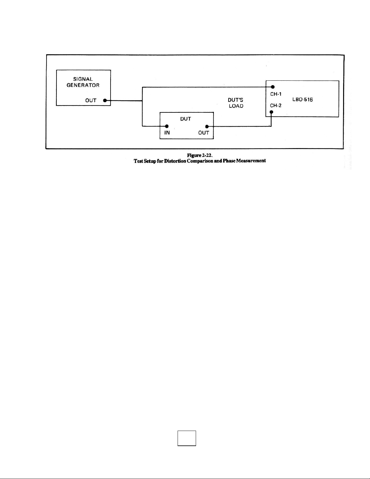
6. Move the off-screen trace back on the CRT with its vertical POSITION control, precisely centering it vertically. Use the associated VOLTS/DIV switch (10) and VARIABLE control (11) to adjust its amplitude to exactly 6 vertical divisions.

7. The horizontal distance between corresponding points on the waveform is the phase difference. For example, in the Figure 2-19 illustration the phase difference is 6 minor divisions, or

°.

You can use the X FINE control (30) to align one of the mid-cycle zero crossings with a graticule calibration to facilitate this measurement.

8. If the phase difference is less than 50° (one major division), pull the A VARIABLE (X10 MAG) control (26) outwards and use the horizontal POSITION control (if needed) to position the measurement area back on screen. With 1 OX magnification, each major horizontal division is 5% and each

minor division is 1

Lissajous Pattern Method.

with sine waves. Measurements are possible at frequencies up to 3 MHz, the bandwidth of the horizontal amplifier. However, for maximum accuracy, measurements of small phase differences should be limited to below 100 kHz.

To measure phase difference by the Lissajous pattern

method, proceed as follows:

1. Depress the X-Y switch (20).

CAUTION:

undetected spot damage the CRT phosphor.

2. Ensure that the CH-2 INV switch (19) is out. This will introduce a 180° error if pushed in.

3. Connect one signal to the CH-1 or X IN connector (14), and the other signal to the CH-2 or Y IN connector (15).

4. Center the trace vertically with the CH-2 vertical POSITION control (18), and adjust the CH-2 VOLTS/DIV switch (10) and VARIABLE control (I1) for a trace height of exactly 6 divisions (the 100% and 0% graticule lines tangent to the trace).

5. Adjust the CH- 1 VOLTS/DIV control (10) for the largest possible on-screen display.

Precisely

POSITION control (29) or X-FINE control (30).

center the trace horizontally with the horizontal

°.

This method is used primarily

Reduce the trace intensity, lest the

7. Count the number of divisions subtended by the trace along the central vertical graticule line (dimension B in Figure 220a). You can now shift the trace vertically with the CH-2 or Y POSITION control to a major division line for easier counting.

8. The phase difference (angle equal to the arc sine of dimension B÷A (the Step 7 number divided by 6). For example, the Step 7 value of the Figure 220a pattern is 2.0. Dividing this by 6 yields .3334, whose arc sine is 19.5 degrees.

9. The simple formula in Figure 2-20a works for angles less than 90°. For angles over 90° (leftward tilt), add 90° to the

angle found in Step 7. Figure 2-20b shows the Lissajous patterns of various phase angles; use this as a guide in de-

termining whether or not to add the additional 90

10. The sine-to-angle conversion can be accomplished by using

trig tables or a trig calculator. However, if the sine is between 0.1 and 1.0, you can use the Figure 2-21 nomograph. Simply lay a ruler on the nomograph so its edge passes through the cross mark and the number of divisions measured in Step 7 (B dimension). When this is done the edge will also intersect the phase-angle column.

2-4-5 Distortion Comparison

The dual-trace feature of the LBO-516 offers a quick method

of checking for distortion caused by a signal-processing device (such as an amplifier). To do this, proceed as follows:

1. Connect the output of the signal generator (of frequency

suitable to the device under test) to the CH- 1 IN connector (14) and the input of the device under test (DUT).

2. Connect the CH-2 IN connector (15) to the output of the device or its load (see Figure 2-22)

3. Increase the signal to the DUT until the channel 2 trace or an RMS AC voltmeter indicates the desired output level.

4. If the DUT has reversed the phase, press the CH-2 INV pushbutton (19).

) between the two signals is

°.

Page 30

5. Superimpose the two traces with the vertical POSITION controls (17) and (18), and use the VARIABLE VOLTS/ DIV control (11) of the larger trace to achieve the best trace match.

6. Any

2-4-6 Frequency Measurements

frequency counter is obviously the first choice. However, an oscilloscope can be used in either of two ways to measure frequency when a counter is not available, or modulation and/or noise makes the counter unusable.

Simply measure the period "t" of the unknown signal as instructed in frequency "f" using the formula f = 1/t. If a calculator is available, simply enter the period and press the 1/x key. Period in seconds (S) yields frequency in hertz (Hz); period in milliseconds (mS) yields frequency in kilohertz (kHz); period in microseconds (PS) yields frequency in megahertz (MHz). The accuracy of this technique is limited by the timebase calibration accuracy (see Table of Specifications).

frequency-ratio method, the unknown frequency is compared to a known frequency (from a calibrated signal generator). The two signals are fed to the oscilloscope operating in its X-Y mode, and the signal generator frequency is varied until a recognizable Lissajous pattern appears. The pattern shape indicates the ratio between the two frequencies. When the generator frequency is multiplied by this ratio, the unknown frequency will be determined. This method is usable for frequencies up to 3 MHz.

follows:

1. Set up the LBO-516 for X-Y operation (paragraph 2-3-11).

2. Connect the output of a signal generator having accurate

3. Adjust the CH- 1 VOLTS/DIV switch (10) for about 6 divi-

4. Connect the signal with the unknown frequency to the CH-2

5. Adjust the CH-2 VOLTS/DIV switch (10) for about 6 divi-

6. Vary the frequency of the signal generator until the scope

uniform horizontal

phase difference (described in paragraph 2-4-4). Any other differences in shape indicate distortion caused by the DUT, such as slew rate or frequency distortion, ringing, etc.

When a precise determination of frequency is needed, a

Reciprocal Method. Frequency is the reciprocal of period.

2-4-3 Time Interval Measurements

Comparison Method. In the frequency-comparison or

To measure frequency by the comparison method, proceed as

frequency calibration to the CH-1 or X IN connector (14).

sions horizontal deflection.

or Y IN connector (15).

sions vertical deflection.

display resembles a circle, an ellipse, or a diagonal line. When this occurs the unknown frequency is the same as the signal generator frequency (which can be read from its dial). The accuracy of this technique depends on the signal generator's calibration accuracy.

displacement of the traces is simply

, and calculate the

NOTE: While many other ratios are theoretically possible, drift in either signal frequency makes more complex Lissajous patterns nearly impossible to read.

2-4-7 Risetime Measurement

Risetime is the time required for the leading edge of a pulse to rise from 10% to 90% of the total pulse amplitude. Falltime is the time required for the trailing edge of a pulse to drop from 90% of total pulse amplitude to 10%. Risetime and falltime, which may be collectively called transition time, are measured in essentially the same manner. To measure rise and fall time, proceed as follows:

1. Connect the pulse to be measured to the CH- 1 IN connector (14) and set the AC/GND/DC switch (16) to AC.

2. Adjust the A TIME/DIV switch (24) to display about 2 cycles

of the pulse. Make certain the associated VARIABLE control

(11) is rotated fully clockwise and de-tented in its CAL'D

position.

3. Center the pulse vertically with the channel 1 vertical

POSITION control (17).

4. Adjust the channel 1 VOLTS/DIV switch (10) to make the

positive pulse peak exceed the 100% graticule line, and the

negative pulse peak exceed the 0% line, then rotate the

VARIABLE control (11) counterclockwise until the positive

and negative pulse peaks rest exactly on the 100% and 0%

graticule lines. (See Figure 2-23).

5. Use the horizontal POSITION (29) and X-FINE (30) controls

to shift the trace so the leading edge passes through the

intersection of the 10% and central vertical graticule lines.

6. If the risetime is slow compared to the period, no further

control manipulations are necessary. If the risetime is fast

(leading edge almost vertical), pull the A VARIABLE (X10

MAG) control (26) and reposition the trace as in Step 5. (See

Figure 2-23b.)

7. Count the number of horizontal divisions between the central

vertical line (10% point) and the intersection of the trace with

the 90% line.

8. Multiply the number of divisions counted in Step 7 by the

setting of the A TIME/DIV switch to find the measured

risetime. If Xl0 magnification was used, divide the

TIME/DIV setting by 10. For example, if the A timebase

setting in Figure 2-23 was .1/PS (100 KS), the risetime would

be 36 nanoseconds (100 KS ÷ 10 = 10 KS; 10 KS x 3.6 div =

36 KS).

9. To measure falltime, simply shift the trace horizontally until

a trailing edge passes through the 10% and central vertical

graticule lines, and repeat Steps 7 and 8.

10. The rise and fall times measured thus far include the 3.5 KS

transition times of the LBO-516 (about 5 KS with probe).

These errors are negligible if the measured rise and fall times

are 20 KS or longer. For shorter transition times, correct the

measured rise and fall times using one of the following

formulas:

Page 31

2-4-8 -- 3 dB Bandwidth Measurement

Bandwidth measurement usually involves finding the -3 dB response point in the frequency-response curve of a circuit or device. This can easily be determined without the need for calculations or dB conversions by using the following "trick":

1. Connect the output of a constant-amplitude signal generator

(of appropriate frequency range) to the input of the de-vice-

under test (DUT). Connect the output of the DUT to the

CH-1 IN connector (14).

2. Set the generator to a frequency

the DUT, then adjust the generator output level to produce

the desired DUT output level.

3. Set the CH-1 VOLTS/DIV control (10) to the

that produces

4. Use the CH-1 VARIABLE VOLTS/DIV control (11) and

CH-1 vertical POSITION control (17) to make the trace

height

and bottom-most graticule lines.

5. Increase the generator frequency until the trace height de-

creases to exactly 5 divisions. This is the upper -3 dB re-

sponse point. The frequency can be determined from the

signal-generator dial, or with a frequency counter connected

to the CH-1 OUTPUT connector (13).

6. Restore the generator to its Step 2 frequency, then decrease

the generator frequency until the trace height decreases to

exactly 5 divisions. This is the lower -3 dB response point.

over 7 divisions

exactly

7 divisions, and touching the second highest

well within

trace height.

the passband of

highest setting

Leader LBO-516 User Manual

Specifications and Main Features

Frequently Asked Questions

User Manual