IBM 170 Servers, 7xx Servers, AS/400 RISC Server User Manual

IBM Power Systems

Performance Capabilities Reference

IBM i operating system Version 6.1

January/April/October 2008

This document is intended for use by qualified performance related programmers or analysts from IBM, IBM Business Partners and IBM customers using the IBM Power running IBM i operating system. Information in this document may be readily shared with IBM i customers to understand the performance and tuning factors in IBM i operating system

6.1 and earlier where applicable. For the latest updates and for the latest on IBM i

performance information, please refer to the Performance Management Website:

http://www.ibm.com/systems/i/advantages/perfmgmt/index.html

Requests for use of performance information by the technical trade press or consultants should be directed to Systems Performance Department V3T, IBM Rochester Lab, in Rochester, MN. 55901 USA.

IBM i 6.1 Performance Capabilities Reference - January/April/October 2008

Systems platform

Note!

Before using this information, be sure to read the general information under “Special Notices.”

Twenty Fifth Edition (January/April/October 2008) SC41-0607-13

This edition applies to IBM i operating System V6.1 running on IBM Power Systems.

You can request a copy of this document by download from IBM i Center via the System i Internet site at:

http://www.ibm.com/systems/i/

available on the IBM iSeries Internet site in the "On Line Library", at: http://publib.boulder.ibm.com/pubs/html/as400/online/chgfrm.htm.

Documents are viewable/downloadable in Adobe Acrobat (.pdf) format. Approximately 1 to 2 MB download. Adobe Acrobat reader plug-in is available at: http://www.adobe.com

To request the CISC version (V3R2 and earlier), enter the following command on VM:

REQUEST V3R2 FROM FIELDSIT AT RCHVMW2 (your name)

To request the IBM iSeries Advanced 36 version, enter the following command on VM:

TOOLCAT MKTTOOLS GET AS4ADV36 PACKAGE

Note to U.S. Government Users -- Documentation related to restricted rights -- Use, duplication, or disclosure is subject to restrictions set forth in GSA ADP Schedule Contract with IBM Corp.

. The Version 5 Release 1 and Version 4 Release 5 Performance Capabilities Guides are also

IBM i 6.1 Performance Capabilities Reference - January/April/October 2008

Table of Contents

2.1 Overview

2.1.1 Interactive Indicators and Metrics

2.1.2 Disclaimer and Remaining Sections

2.1.3 V5R3

2.1.4 V5R2 and V5R1

2.2 Server Model Behavior

2.2.1 In V4R5 - V5R2

2.2.2 Choosing Between Similarly Rated Systems

2.2.3 Existing Older Models

2.3 Server Model Differences

2.4 Performance Highlights of Model 7xx Servers

2.5 Performance Highlights of Model 170 Servers

2.6 Performance Highlights of Custom Server Models

2.7 Additional Server Considerations

2.8 Interactive Utilization

2.9 Server Dynamic Tuning (SDT)

2.10 Managing Interactive Capacity

2.11 Migration from Traditional Models

2.12 Upgrade Considerations for Interactive Capacity

2.13 iSeries for Domino and Dedicated Server for Domino Performance Behavior

2.13.1 V5R2 iSeries for Domino & DSD Performance Behavior updates

2.13.2 V5R1 DSD Performance Behavior

3.1 Effect of CPU Speed on Batch

3.2 Effect of DASD Type on Batch

3.3 Tuning Parameters for Batch

4.1 New for i5/OS V6R1

i5/OS V6R1 SQE Query Coverage

4.2 DB2 i5/OS V5R4 Highlights

i5/OS V5R4 SQE Query Coverage

4.3 i5/OS V5R3 Highlights

i5/OS V5R3 SQE Query Coverage Partitioned Table Support

4.4 V5R2 Highlights - Introduction of the SQL Query Engine

4.5 Indexing

4.6 DB2 Symmetric Multiprocessing feature

4.7 DB2 for i5/OS Memory Sharing Considerations

4.8 Journaling and Commitment Control

4.9 DB2 Multisystem for i5/OS

4.10 Referential Integrity

4.11 Triggers

4.12 Variable Length Fields

4.13 Reuse Deleted Record Space

4.14 Performance References for DB2

.....................................................................

.............................................

............................................

....................................................................

...........................................................

..........................................................

............................................................

......................................

.......................................................

........................................................

........................................

.....................................

..................................................

...........................................................

....................................................

...................................................

................................................

.....................................

....................

............................................

.....................................................

....................................................

......................................................

.............................................................

..................................................

......................................................

..................................................

...........................................................

..................................................

........................................................

...............................

......................................................................

.............................................

.......................................

................................................

.......................................................

............................................................

.....................................................................

..........................................................

.....................................................

.................................................

.............

10Special Notices ....................................................................

12Purpose of this Document ...........................................................

13Chapter 1. Introduction ............................................................

14Chapter 2. iSeries and AS/400 RISC Server Model Performance Behavior .................

14 14 15 15 16 16 16 17 17 19 21 22 23 23 24 25 28 31 33 34 34 34

38Chapter 3. Batch Performance ......................................................

38 38 39

41Chapter 4. DB2 for i5/OS Performance ...............................................

41 41 44 44 45 45 47 49 51 52 53 53 56 57 58 59 61 62

IBM i 6.1 Performance Capabilities Reference - January/April/October 2008

5.2 Communication Performance Test Environment

5.5 TCP/IP Secure Performance

5.6 Performance Observations and Tips

5.7 APPC, ICF, CPI-C, and Anynet

.......................................................

.................................................

....................................................

5.8 HPR and Enterprise extender considerations

5.9 Additional Information

6.1 HTTP Server (powered by Apache)

6.2 PHP - Zend Core for i

6.3 WebSphere Application Server

6.4 IBM WebFacing

...........................................................

.................................................

............................................................

....................................................

..............................................................

.......................................

..........................................

6.5 WebSphere Host Access Transformation Services (HATS)

6.6 System Application Server Instance

6.7 WebSphere Portal

6.8 WebSphere Commerce

..............................................................

..........................................................

6.9 WebSphere Commerce Payments

6.10 Connect for iSeries

7.1 Introduction

...................................................................

7.2 What’s new in V6R1

...........................................................

............................................................

7.3 IBM Technology for Java (32-bit and 64-bit)

Native Code Garbage Collection

7.4 Classic VM (64-bit)

JIT Compiler Garbage Collection Bytecode Verification

..................................................................

............................................................

..................................................................

............................................................

...........................................................

7.5 Determining Which JVM to Use

7.6 Capacity Planning

General Guidelines

.............................................................

7.7 Java Performance – Tips and Techniques

Introduction

..................................................................

i5/OS Specific Java Tips and Techniques Classic VM-specific Tips

........................................................

Java Language Performance Tips Java i5/OS Database Access Tips

Resources

.......................................................................

8.1 System i Cryptographic Solutions

8.2 Cryptography Performance Test Environment

8.3 Software Cryptographic API Performance

8.4 Hardware Cryptographic API Performance

...............................................

.................................................

.........................................

..................................................

...........................................

............................................

.................................................

..................................................

........................................

..........................................

8.5 Cryptography Observations, Tips and Recommendations

8.6 Additional Information

9.1 iSeries NetServer File Serving Performance

10.1 DB2 for i5/OS access with JDBC

JDBC Performance Tuning Tips References for JDBC

.........................................................

.........................................

.................................................

..................................................

..........................................................

..............................

...............................

63Chapter 5. Communications Performance .............................................

65 68 71 73 75 77

78Chapter 6. Web Server and WebSphere Performance ..................................

79 88

93 107 117 119 121 121 122 122

126Chapter 7. Java Performance ......................................................

126 126 127 128 128 129 129 131 132 133 135 135 136 136 137 137 138 141 142

143Chapter 8. Cryptography Performance ..............................................

143 144 145 146 148 149

150Chapter 9. iSeries NetServer File Serving Performance ................................

150

153Chapter 10. DB2 for i5/OS JDBC and ODBC Performance .............................

153 153 154

IBM i 6.1 Performance Capabilities Reference - January/April/October 2008

10.2 DB2 for i5/OS access with ODBC

References for ODBC

...........................................................

11.1 Domino Workload Descriptions

11.2 Domino 8

11.3 Domino 7

11.4 Domino 6

...................................................................

Notes client improvements with Domino 6 Domino Web Access client improvements with Domino 6

11.5 Response Time and Megahertz relationship

11.6 Collaboration Edition and Domino Edition offerings

11.7 Performance Tips / Techniques

11.8 Domino Web Access

..........................................................

11.9 Domino Subsystem Tuning

11.10 Performance Monitoring Statistics

11.11 Main Storage Options

........................................................

11.12 Sizing Domino on System i

11.13 LPAR and Partial Processor Considerations

11.14 System i NotesBench Audits and Benchmarks

12.1 Introduction

.................................................................

................................................

.................................................

...........................................

...............................

.......................................

.................................

..................................................

.....................................................

...............................................

...................................................

.......................................

......................................

12.2 Performance Improvements for WebSphere MQ V5.3 CSD6

12.3 Test Description and Results

12.4 Conclusions, Recommendations and Tips

13.1 Summary

Key Ideas

....................................................................

13.2 Basic Requirements -- Where Linux Runs

13.3 Linux on iSeries Technical Overview

Linux on iSeries Architecture Linux on iSeries Run-time Support

13.4 Basic Configuration and Performance Questions

13.5 General Performance Information and Results

Computational Performance -- C-based code Computational Performance -- Java Web Serving Performance Network Operations

............................................................

Gcc and High Optimization (gcc compiler option -O3) The Gcc Compiler, Version 3

13.6 Value of Virtual LAN and Virtual Disk

Virtual LAN Virtual Disk

..................................................................

13.7 DB2 UDB for Linux on iSeries

13.8 Linux on iSeries and IBM eServer Workload Estimator

13.9 Top Tips for Linux on iSeries Performance

14.1 Internal (Native) Attachment.

14.1.0 Direct Attach (Native)

14.1.1 Hardware Characteristics

14.1.2 iV5R2 Direct Attach DASD

14.1.3 571B

.................................................................

....................................................

..........................................

..............................................

.....................................................

.................................................

.....................................

.......................................

........................................

...............................................

.......................................................

.................................

.....................................................

............................................

...................................................

...............................

.........................................

...................................................

........................................................

...............................................

...................................................

...........................

155 157

158Chapter 11. Domino on i ..........................................................

159 160 160 161 161 162 163 164 164 167 168 168 169 172 173 174

175Chapter 12. WebSphere MQ for iSeries .............................................

175 175 176 176

178Chapter 13. Linux on iSeries Performance ...........................................

178 178 178 179 179 180 181 182 182 183 183 184 184 185 185 185 185 186 187 187

191Chapter 14. DASD Performance ...................................................

191 192 192 193 195

IBM i 6.1 Performance Capabilities Reference - January/April/October 2008

14.1.3.1 571B RAID5 vs RAID6 - 10 15K 35GB DASD

14.1.3.2 571B IOP vs IOPLESS - 10 15K 35GB DASD

14.1.4 571B, 5709, 573D, 5703, 2780 IOA Comparison Chart

................................

.................................

..........................

14.1.5 Comparing Current 2780/574F with the new 571E/574F and 571F/575B NOTE: iV5R3 has support for the features in this section but all of our performance measurements were done on iV5R4 systems. For information on the

supported features see the IBM Product Announcement Letters. ..........................

14.1.6 Comparing 571E/574F and 571F/575B IOP and IOPLess

14.1.7 Comparing 571E/574F and 571F/575B RAID5 and RAID6 and Mirroring

14.1.8 Performance Limits on the 571F/575B

.......................................

14.1.9 Investigating 571E/574F and 571F/575B IOA, Bus and HSL limitations.

14.1.10 Direct Attach 571E/574F and 571F/575B Observations

14.2 New in iV5R4M5

14.2.1 9406-MMA CEC vs 9406-570 CEC DASD

14.2.2 RAID Hot Spare

14.2.3 12X Loop Testing

14.3 New in iV6R1M0

14.3.1 Encrypted ASP

14.3.2 57B8/57B7 IOA

14.3.3 572A IOA

14.4 SAN - Storage Area Network (External)

14.5.1 General VIOS Considerations

14.5.1.1 Generic Concepts

14.5.1.2 Generic Configuration Concepts

.............................................................

....................................

..........................................................

.........................................................

.............................................................

...........................................................

..........................................................

...............................................................

...........................................

..................................................

.......................................................

..............................................

.........................

...........

............

.........................

14.5.1.3 Specific VIOS Configuration Recommendations -- Traditional (non-blade)

Machines ........................................................................

14.5.1.3 VIOS and JS12 Express and JS22 Express Considerations

14.5.1.3.1 BladeCenter H JS22 Express running IBM i operating system/VIOS

14.5.1.3.2 BladeCenter S and JS12 Express

.........................................

14.5.1.3.3 JS12 Express and JS22 Express Configuration Considerations

14.5.1.3.4 DS3000/DS4000 Storage Subsystem Performance Tips

14.6 IBM i operating system 5.4 Virtual SCSI Performance

14.6.1 Introduction

14.6.2 Virtual SCSI Performance Examples

14.6.2.1 Native vs. Virtual Performance

................................................................

.........................................

...........................................

14.6.2.2 Virtual SCSI Bandwidth-Multiple Network Storage Spaces

14.6.2.3 Virtual SCSI Bandwidth-Network Storage Description (NWSD) Scaling

14.6.2.4 Virtual SCSI Bandwidth-Disk Scaling

14.6.3 Sizing

....................................................................

14.6.3.1 Sizing when using Dedicated Processors

14.6.3.2 Sizing when using Micro-Partitioning

14.6.3.3 Sizing memory

.........................................................

14.6.4 AIX Virtual IO Client Performance Guide

14.6.5 Performance Observations and Tips

14.6.6 Summary

.................................................................

15.1 Supported Backup Device Rates

.............................................

.................................................

15.2 Save Command Parameters that Affect Performance

Use Optimum Block Size (USEOPTBLK) Data Compression (DTACPR) Data Compaction (COMPACT)

....................................................

...................................................

.......................................

....................................

......................................

........................................

.................................

............................................

..........................

..........

.................

.......................

.............................

......................

............

195 195 196

198 199 200 202 203 205 206 206 207 208 209 209 211 213 214 216 216 217

220 222 222 227 228 229 231 233 234 235 235 236 237 238 238 240 241 242 242 242

243Chapter 15. Save/Restore Performance ..............................................

243 244 244 244 244

IBM i 6.1 Performance Capabilities Reference - January/April/October 2008

15.3 Workloads

15.4 Comparing Performance Data

15.5 Lower Performing Backup Devices

15.6 Medium & High Performing Backup Devices

15.7 Ultra High Performing Backup Devices

15.8 The Use of Multiple Backup Devices

15.9 Parallel and Concurrent Library Measurements

15.9.1 Hardware (2757 IOAs, 2844 IOPs, 15K RPM DASD)

15.9.2 Large File Concurrent

15.9.3 Large File Parallel

15.9.4 User Mix Concurrent

15.10 Number of Processors Affect Performance

15.11 DASD and Backup Devices Sharing a Tower

15.12 Virtual Tape

15.13 Parallel Virtual Tapes

15.14 Concurrent Virtual Tapes

15.15 Save and Restore Scaling using a Virtual Tape Drive.

..................................................................

...................................................

...............................................

......................................

...........................................

.............................................

.....................................

...........................

....................................................

.......................................................

.....................................................

........................................

......................................

................................................................

.........................................................

......................................................

................................

15.16 Save and Restore Scaling using 571E IOAs and U320 15K DASD units to a

3580 Ultrium 3 Tape Drive. .........................................................

15.17 High-End Tape Placement on System i

..........................................

15.18 BRMS-Based Save/Restore Software Encryption and DASD-Based ASP

Encryption ......................................................................

15.19 5XX Tape Device Rates

.......................................................

15.20 5XX Tape Device Rates with 571E & 571F Storage IOAs and 4327 (U320)

Disk Units .......................................................................

15.21 5XX DVD RAM and Optical Library

15.23 9406-MMA DVD RAM

.....................................................

15.24 9406-MMA 576B IOPLess IOA

16.1 IPL Performance Considerations

16.2 IPL Test Description

...........................................................

16.3 9406-MMA System Hardware Information

16.3.1 Small system Hardware Configuration

16.3.2 Large system Hardware Configurations

16.4 9406-MMA IPL Performance Measurements (Normal)

16.5 9406-MMA IPL Performance Measurements (Abnormal)

16.6 NOTES on MSD

..............................................................

16.6.1 MSD Affects on IPL Performance Measurements

16.7 5XX System Hardware Information

16.7.1 5XX Small system Hardware Configuration

16.7.2 5XX Large system Hardware Configuration

16.8 5XX IPL Performance Measurements (Normal)

16.9 5XX IPL Performance Measurements (Abnormal)

16.10 5XX IOP vs IOPLess effects on IPL Performance (Normal)

16.11 IPL Tips

17.1 Introduction

...................................................................

..................................................................

17.2 Effects of Windows and Linux loads on the host system

17.2.1 IXS/IXA Disk I/O Operations:

17.2.2 iSCSI Disk I/O Operations:

17.2.3 iSCSI virtual I/O private memory pool

............................................

..............................................

.................................................

.........................................

.......................................

......................................

...............................

..............................

................................

...............................................

....................................

......................................

....................................

...........................

...............................

...............................................

.................................................

........................................

245 246 247 247 247 248 249 249 250 251 252 253 254 255 257 258 259

260 262

263 265

267 268 270 271

273Chapter 16 IPL Performance ......................................................

273 273 274 274 274 275 275 276 276 277 277 277 278 278 279 279

280Chapter 17. Integrated BladeCenter and System x Performance .........................

280 281 281 282 283

IBM i 6.1 Performance Capabilities Reference - January/April/October 2008

17.2.4 Virtual Ethernet Connections:

17.2.5 IXS/IXA IOP Resource:

17.3 System i memory rules of thumb for IXS/IXA and iSCSI attached servers.

17.3.1 IXS and IXA attached servers:

17.3.2 iSCSI attached servers:

17.4 Disk I/O CPU Cost

............................................................

....................................................

17.4.1 Further notes about IXS/IXA Disk Operations

17.5 Disk I/O Throughput

...........................................................

17.6 Virtual Ethernet CPU Cost and Capacities

17.6.1 VE Capacity Comparisons

17.6.2 VE CPW Cost

17.6.3 Windows CPU Cost

...........................................................

.......................................................

17.7 File Level Backup Performance

17.8 Summary

....................................................................

17.9 Additional Sources of Information

18.1 Introduction

V5R3 Information V5R2 Additions General Tips V5R1 Additions

18.2 Considerations

..................................................................

..............................................................

................................................................

..................................................................

................................................................

18.3 Performance on a 12-way system

18.4 LPAR Measurements

18.5 Summary

....................................................................

..........................................................

..............................................

...................................................

................

...............................................

..................................

..........................................

.................................................

..................................................

................................................

.................................................

19.1 Public Benchmarks (TPC-C, SAP, NotesBench, SPECjbb2000, VolanoMark)

19.2 Dynamic Priority Scheduling

19.3 Main Storage Sizing Guidelines

19.4 Memory Tuning Using the QPFRADJ System Value

19.5 Additional Memory Tuning Techniques

19.6 User Pool Faulting Guidelines

19.7 AS/400 NetFinity Capacity Planning

20.1 Adjusting Your Performance Tuning for Threads

20.2 General Performance Guidelines -- Effects of Compilation

....................................................

.................................................

.................................

...........................................

...................................................

..............................................

....................................

.............................

20.3 How to Design for Minimum Main Storage Use (especially with Java, C, C++)

Theory -- and Practice System Level Considerations Typical Storage Costs A Brief Example Which is more important? A Short but Important Tip about Data Base A Final Thought About Memory and Competitiveness

20.4 Hardware Multi-threading (HMT)

HMT Described HMT and SMT Compared and Contrasted Models With/Without HMT

20.5 POWER6 520 Memory Considerations

20.6 Aligning Floating Point Data on Power6

..........................................................

.....................................................

...........................................................

...............................................................

.......................................................

..........................................

..................................

................................................

...............................................................

...........................................

.......................................................

............................................

...........................................

.............

284 285 285 285 285 286 287 288 289 290 291 291 292 293 293

295Chapter 18. Logical Partitioning (LPAR) ............................................

295 295 295 295 296 296 297 300 301

302Chapter 19. Miscellaneous Performance Information ..................................

302 304 307 307 308 310 311

314Chapter 20. General Performance Tips and Techniques ...............................

314 316 317 317 318 318 319 320 321 321 322 322 323 323 324 325

327Chapter 21. High Availability Performance ...........................................

IBM i 6.1 Performance Capabilities Reference - January/April/October 2008

21.1 Switchable IASP’s

21.2 Geographic Mirroring

22.1 Overview

....................................................................

22.2 Merging PM for System i data into the Estimator

22.3 Estimator Access

22.4 What the Estimator is Not

A.1 Commercial Processing Workload - CPW A.2 Compute Intensive Workload - CIW

B.1 Performance Data Collection Services B.2 Batch Modeling Tool (BCHMDL).

C.1 V6R1 Additions (October 2008) C.2 V6R1 Additions (August 2008) C.3 V6R1 Additions (April 2008) C.4 V6R1 Additions (January 2008) C.5 V5R4 Additions (July 2007)

............................................................

..........................................................

....................................

..............................................................

.......................................................

..........................................

..............................................

.............................................

.................................................

..................................................

....................................................

..................................................

....................................................

C.6 V5R4 Additions (January/May/August 2006 and January/April 2007) C.7 V5R3 Additions (May, July, August, October 2004, July 2005)

C.7.1 IBM

~®

C.8 V5R2 Additions (February, May, July 2003)

C.8.1 iSeries Model 8xx Servers

i5 Servers

..................................................

........................................

..................................................

C.8.2 Model 810 and 825 iSeries for Domino (February 2003) C.9 V5R2 Additions

C.9.1 Base Models 8xx Servers C.9.2 Standard Models 8xx Servers

C.10 V5R1 Additions

C.10.1 Model 8xx Servers C.10.2 Model 2xx Servers C.10.3 V5R1 Dedicated Server for Domino C.10.4 Capacity Upgrade on-demand Models

...............................................................

..................................................

................................................

..............................................................

.......................................................

.........................................

.......................................

C.10.4.1 CPW Values and Interactive Features for CUoD Models

C.11 V4R5 Additions

C.11.1 AS/400e Model 8xx Servers C.11.2 Model 2xx Servers C.11.3 Dedicated Server for Domino C.11.4 SB Models

C.12 V4R4 Additions

C.12.1 AS/400e Model 7xx Servers C.12.2 Model 170 Servers

C.13 AS/400e Model Sxx Servers C.14 AS/400e Custom Servers C.15 AS/400 Advanced Servers C.16 AS/400e Custom Application Server Model SB1 C.17 AS/400 Models 4xx, 5xx and 6xx Systems C.18 AS/400 CISC Model Capacities

..............................................................

................................................

.......................................................

..............................................

.............................................................

..............................................................

................................................

......................................................

...................................................

.......................................................

.....................................................

....................................

.........................................

.................................................

.........................

..............................

.......................

....................

327 329

334Chapter 22. IBM Systems Workload Estimator ......................................

334 335 335 335

337Appendix A. CPW and CIW Descriptions ............................................

337 339

341Appendix B. System i Sizing and Performance Data Collection Tools ....................

342 343

345Appendix C. CPW and MCU Relative Performance Values for System i ..................

346 347 347 348 349 349 351 351 353 353 354 354 354 354 355 356 357 357 357 358 360 360 361 361 362 362 362 363 365 365 365 366 367 368

IBM i 6.1 Performance Capabilities Reference - January/April/October 2008

Special Notices

DISCLAIMER NOTICE

Performance is based on measurements and projections using standard IBM benchmarks in a controlled environment. This information is presented along with general recommendations to assist the reader to have a better understanding of IBM(*) products. The actual throughput or performance that any user will experience will vary depending upon considerations such as the amount of multiprogramming in the user's job stream, the I/O configuration, the storage configuration, and the workload processed. Therefore, no assurance can be given that an individual user will achieve throughput or performance improvements equivalent to the ratios stated here.

All performance data contained in this publication was obtained in the specific operating environment and under the conditions described within the document and is presented as an illustration. Performance

obtained in other operating environments may vary and customers should conduct their own testing.

Information is provided "AS IS" without warranty of any kind.

The use of this information or the implementation of any of these techniques is a customer responsibility and depends on the customer's ability to evaluate and integrate them into the customer's operational environment. While each item may have been reviewed by IBM for accuracy in a specific situation, there is no guarantee that the same or similar results will be obtained elsewhere. Customers attempting to adapt these techniques to their own environments do so at their own risk.

All statements regarding IBM future direction and intent are subject to change or withdrawal without notice, and represent goals and objectives only. Contact your local IBM office or IBM authorized reseller for the full text of the specific Statement of Direction.

Some information addresses anticipated future capabilities. Such information is not intended as a definitive statement of a commitment to specific levels of performance, function or delivery schedules with respect to any future products. Such commitments are only made in IBM product announcements. The information is presented here to communicate IBM's current investment and development activities as a good faith effort to help with our customers' future planning.

IBM may have patents or pending patent applications covering subject matter in this document. The furnishing of this document does not give you any license to these patents. You can send license inquiries, in writing, to the IBM Director of Commercial Relations, IBM Corporation, Purchase, NY

10577.

Information concerning non-IBM products was obtained from a supplier of these products, published announcement material, or other publicly available sources and does not constitute an endorsement of such products by IBM. Sources for non-IBM list prices and performance numbers are taken from publicly available information, including vendor announcements and vendor worldwide homepages. IBM has not tested these products and cannot confirm the accuracy of performance, capability, or any other claims related to non-IBM products. Questions on the capability of non-IBM products should be addressed to the supplier of those products.

IBM i 6.1 Performance Capabilities Reference - January/April/October 2008

The following terms, which may or may not be denoted by an asterisk (*) in this publication, are trademarks of the IBM Corporation.

Operating System/400System/370iSeries or AS/400 i5/OS IPDSC/400 Application System/400COBOL/400OS/400 OfficeVisionRPG/400System i5 Facsimile Support/400CallPathSystem i Distributed Relational Database ArchitectureDRDAPS/2 Advanced Function PrintingSQL/400OS/2 Operational AssistantImagePlusDB2 Client SeriesVTAMAFP Workstation Remote IPL/400APPNIBM Advanced Peer-to-Peer NetworkingSystemViewSQL/DS OfficeVision/400ValuePoint400 iSeries Advanced Application ArchitectureDB2/400CICS ADSTAR Distributed Storage Manager/400ADSM/400S/370 IBM Network StationAnyNet/400RPG IV Lotus, Lotus Notes, Lotus Word Pro, Lotus 1-2-3AIX POWER4+POWER4Micro-partitioning

Systems

POWER5+POWER5POWER POWER6+POWER6Power PowerTM Systems SoftwarePowerTM Systems SoftwarePowerPC

The following terms, which may or may not be denoted by a double asterisk (**) in this publication, are trademarks or registered trademarks of other companies as follows:

Transaction Processing Performance CouncilTPC Benchmark Transaction Processing Performance CouncilTPC-A, TPC-B Transaction Processing Performance CouncilTPC-C, TPC-D Microsoft CorporationODBC, Windows NT Server, Access Microsoft CorporationVisual Basic, Visual C++ Adobe Systems IncorporatedAdobe PageMaker Borland International IncorporatedBorland Paradox Corel CorporationCorelDRAW! Borland InternationalParadox Satelite Software InternationalWordPerfect BGS Systems, Inc.BEST/1 NovellNetWare Compaq Computer CorporationCompaq Compaq Computer CorporationProliant Business Application Performance CorporationBAPCo Gaphics Software Publishing CorporationHarvard Hewlett Packard CorporationHP-UX Hewlett Packard CorporationHP 9000 Intersolve, Inc.INTERSOLV Intersolve, Inc.Q+E Novell, Inc.Netware Systems Performance Evaluation CooperativeSPEC UNIX Systems LaboratoriesUNIX WordPerfect CorporationWordPerfect Powersoft CorporationPowerbuilder Gupta CorporationSQLWindows Ziff-Davis Publishing CompanyNetBench Digital Equipment CorporationDEC Alpha

Microsoft, Windows, Windows 95, Windows NT, Internet Explorer, Word, Excel, and Powerpoint, and the Windows logo are trademarks of Microsoft Corporation in the United States, other countries, or both. Intel, Intel Inside (logos), MMX and Pentium are trademarks of Intel Corporation in the United States, other countries, or both. Linux is a trademark of Linus Torvalds in the United States, other countries, or both. Java and all Java-based trademarks are trademarks of Sun Microsystems, Inc. in the United States, other countries, or both.

Other company, product or service names may be trademarks or service marks of others

IBM i 6.1 Performance Capabilities Reference - January/April/October 2008

Purpose of this Document

The intent of this document is to help provide guidance in terms of IBM i operating system performance, capacity planning information, and tips to obtain optimal performance on IBM i operating system. This document is typically updated with each new release or more often if needed.

This October 2008 edition of the IBM i V6.1 Performance Capabilities Reference Guide is an update to the April 2008 edition to reflect new product functions announced on October 7, 2008.

This edition includes performance information on newly announced IBM Power Systems including Power 520 and Power 550, utilizing POWER6 processor technology. This document further includes information on IBM System i 570 using POWER6 processor technology, IBM i5/OS running on IBM BladeCenter JS22 using POWER6 processor technology, recent System i5 servers (model 515, 525, and

595) featuring new user-based licensing for the 515 and 525 models and a new 2.3GHz model 595, DB2 UDB for iSeries SQL Query Engine Support, Websphere Application Server including WAS V6.1 both with the Classic VM and the IBM Technology for Java (32-bit) VM, WebSphere Host Access Transformation Services (HATS) including the IBM WebFacing Deployment Tool with HATS Technology (WDHT), PHP - Zend Core for i, Java including Classic JVM (64-bit), IBM Technology for Java (32-bit), IBM Technology for Java (64-bit) and bytecode verification, Cryptography, Domino 7, Workplace Collaboration Services (WCS), RAID6 versus RAID5 disk comparisons, new internal storage adapters, Virtual Tape, and IPL Performance.

The wide variety of applications available makes it extremely difficult to describe a "typical" workload. The data in this document is the result of measuring or modeling certain application programs in very specific and unique configurations, and should not be used to predict specific performance for other applications. The performance of other applications can be predicted using a system sizing tool such as IBM Systems Workload Estimator (refer to Chapter 22 for more details on Workload Estimator).

IBM i 6.1 Performance Capabilities Reference - January/April/October 2008

Chapter 1. Introduction

IBM System i and IBM System p platforms unified the value of their servers into a single, powerful lineup of servers based on industry leading POWER6 processor technology with support for IBM i operating system (formerly known as i5/OS), IBM AIX and Linux for Power.

Following along with this exciting unification are a number of naming changes to the formerly named i5/OS, now officially called IBM i operating system. Specifically, recent versions of the operating system are referred to by IBM i operating system 6.1 and IBM i operating system 5.4, formerly i5/OS V6R1 and i5/OS V5R4 respectively. Shortened forms of the new operating system name are IBM i 6.1, i 6.1, i V6.1 iV6R1, and sometimes simply ‘i’. As always, references to legacy hardware and software will commonly use the naming conventions of the time.

The Power 520 Express Edition is the entry member of the Power Systems portfolio, supporting both IBM i 5.4 and IBM i 6.1. The System i 570 is enhanced to enable medium and large enterprises to grow and extend their IBM i business applications more affordably and with more granularity, while offering effective and scalable options for deploying Linux and AIX applications on the same secure, reliable system.

The IBM Power 570 running IBM i offers IBM's fastest POWER6 processors in 2 to 16-way configurations, plus an array of other technology advances. It is designed to deliver outstanding price/performance, mainframe-inspired reliability and availability features, flexible capacity upgrades, and innovative virtualization technologies. New 5.0GHz and 4.4GHz POWER6 processors use the very latest 64-bit IBM POWER processor technology. Each 2-way 570 processor card contains one two-core chip (two processors) and comes with 32 MB of L3 cache and 8 MB of L2 cache.

The CPW ratings for systems with POWER6 processors are approximately 70% higher than equivalent POWER5 systems and approximately 30% higher than equivalent POWER5+ systems. For some compute-intensive applications, the new System i 570 can deliver up to twice the performance of the original 570 with 1.65 GHz POWER5 processors.

The 515 and 525 models introduced in April 2007, introduce user-based licensing for IBM i. For assistance in determining the required number of user licenses, see

ttp://www.ibm.com/systems/i/hardware/515 (model 515) or

h http://www.ibm.com/systems/i/hardware/525 (model 525). User-based licensing is not a

replacement for system sizing; instead, user-based licensing enables appropriate user connectivity to the system. Application environments require different amounts of system resources per user. See Chapter 22 (IBM Systems Workload Estimator) for assistance in system sizing.

Customers who wish to remain with their existing hardware but want to move to IBM i 6.1 may find functional and performance improvements. IBM i 6.1 continues to help protect the customer's investment while providing more function and better price/performance over previous

IBM i 6.1 Performance Capabilities Reference - January/April/October 2008

versions. The primary public performance information web site is found at:

http://www.ibm.com/systems/i/advantages/perfmgmt/index.html

IBM i 6.1 Performance Capabilities Reference - January/April/October 2008

Chapter 2. iSeries and AS/400 RISC Server Model Performance Behavior

2.1 Overview

iSeries and AS/400 servers are intended for use primarily in client/server or other non-interactive work environments such as batch, business intelligence, network computing etc. 5250-based interactive work can be run on these servers, but with limitations. With iSeries and AS/400 servers, interactive capacity can be increased with the purchase of additional interactive features. Interactive work is defined as any job doing 5250 display device I/O. This includes:

All 5250 sessions Any green screen interface Telnet or 5250 DSPT workstations 5250/HTML workstation gateway PC's using 5250 emulation Interactive program debugging

RUMBA/400 Screen scrapers Interactive subsystem monitors Twinax printer jobs BSC 3270 emulation 5250 emulation

PC Support/400 work station function

Note that printer work that passes through twinax media is treated as interactive, even though there is no “user interface”. This is true regardless of whether the printer is working in dedicated mode or is printing spool files from an out queue. Printer activity that is routed over a LAN through a PC print controller are not considered to be interactive.

This explanation is different than that found in previous versions of this document. Previous versions indicated that spooled work would not be considered to be interactive and were in error.

As of January 2003, 5250 On-line Transaction Processing (OLTP) replaces the term “interactive” when referencing interactive CPW or interactive capacity. Also new in 2003, when ordering a iSeries server, the customer must choose between a Standard Package and an Enterprise Package in most cases. The Standard Packages comes with zero 5250 CPW and 5250 OLTP workloads are not supported. However, the Standard Package does support a limited 5250 CPW for a system administrator to manage various aspects of the server. Multiple administrative jobs will quickly exceed this capability. The Enterprise Package does not have any limits relative to 5250 OLTP workloads. In other words, 100% of the server capacity is available for 5250 OLTP applications whenever you need it.

5250 OLTP applications can be run after running the WebFacing Tool of IBM WebSphere Development Studio for iSeries and will require no 5250 CPW if on V5R2 and using model 800, 810, 825, 870, or 890 hardware.

2.1.1 Interactive Indicators and Metrics

Prior to V4R5, there were no system metrics that would allow a customer to determine the overall interactive feature capacity utilization. It was difficult for the customer to determine how much of the total interactive capacity he was using and which jobs were consuming interactive capacity. This got much easier with the system enhancements made in V4R5 and V5R1.

Starting with V4R5, two new metrics were added to the data generated by Collection Services to report the system's interactive CPU utilization (ref file QAPMSYSCPU). The first metric (SCIFUS) is the

IBM i 6.1 Performance Capabilities Reference - January/April/October 2008

interactive utilization - an average for the interval. Since average utilization does not indicate potential problems associated with peak activity, a second metric (SCIFTE) reports the amount of interactive utilization that occurred above threshold. Also, interactive feature utilization was reported when printing a System Report generated from Collection Services data. In addition, Management Central now monitors interactive CPU relative to the system/partition capacity.

Also in V4R5, a new operator message, CPI1479, was introduced for when the system has consistently exceeded the purchased interactive capacity on the system. The message is not issued every time the capacity is reached, but it will be issued on an hourly basis if the system is consistently at or above the limit. In V5R2, this message may appear slightly more frequently for 8xx systems, even if there is no change in the workload. This is because the message event was changed from a point that was beyond the purchased capacity to the actual capacity for these systems in V5R2.

In V5R1, Collection Services was enhanced to mark all tasks that are counted against interactive capacity (ref file QAPMJOBMI, field JBSVIF set to ‘1’). It is possible to query this file to understand what tasks have contributed to the system’s interactive utilization and the CPU utilized by all interactive tasks. Note: the system’s interactive capacity utilization may not be equal to the utilization of all interactive tasks. Reasons for this are discussed in Section 2.10, Managing Interactive Capacity.

With the above enhancements, a customer can easily monitor the usage of interactive feature and decide when he is approaching the need for an interactive feature upgrade.

2.1.2 Disclaimer and Remaining Sections

The performance information and equations in this chapter represent ideal environments. This information is presented along with general recommendations to assist the reader to have a better understanding of the iSeries server models. Actual results may vary significantly.

This chapter is organized into the following sections:

y Server Model Behavior y Server Model Differences y Performance Highlights of New Model 7xx Servers y Performance Highlights of Current Model 170 Servers y Performance Highlights of Custom Server Models y Additional Server Considerations y Interactive Utilization y Server Dynamic Tuning (SDT) y Managing Interactive Capacity y Migration from Traditional Models y Migration from Server Models y Dedicated Server for Domino (DSD) Performance Behavior

2.1.3 V5R3

Beginning with V5R3, the processing limitations associated with the Dedicated Server for Domino (DSD) models have been removed. Refer to section 2.13, “Dedicated Server for Domino Performance Behavior”, for additional information.

IBM i 6.1 Performance Capabilities Reference - January/April/October 2008

2.1.4 V5R2 and V5R1

There were several new iSeries 8xx and 270 server model additions in V5R1 and the i890 in V5R2. However, with the exception of the DSD models, the underlying server behavior did not change from V4R5. All 27x and 8xx models, including the new i890 utilize the same server behavior algorithm that was announced with the first 8xx models supported by V4R5. For more details on these new models, please refer to Appendix C, “CPW, CIW and MCU Values for iSeries”.

Five new iSeries DSD models were introduced with V5R1. In addition, V5R1 expanded the capability of the DSD models with enhanced support of Domino-complementary workloads such as Java Servlets and WebSphere Application Server. Please refer to Section 2.13, Dedicated Server for Domino Performance Behavior, for additional information.

2.2 Server Model Behavior

2.2.1 In V4R5 - V5R2

Beginning with V4R5, all 2xx, 8xx and SBx model servers utilize an enhanced server algorithm that manages the interactive CPU utilization. This enhanced server algorithm may provide significant user benefit. On prior models, when interactive users exceed the interactive CPW capacity of a system, additional CPU usage visible in one or more CFINT tasks, reduces system capacity for all users including client/server. New in V4R5, the system attempts to hold interactive CPU utilization below the threshold where CFINT CPU usage begins to increase. Only in cases where interactive demand exceeds the limitations of the interactive capacity for an extended time (for example: from long-running, CPU-intensive transactions), will overhead be visable via the CFINT tasks. Highlights of this new algorithm include the following: y As interactive users exceed the installed interactive CPW capacity, the response times of those

applications may significantly lengthen and the system will attempt to manage these interactive excesses below a level where CFINT CPU usage begins to increase. Generally, increased CFINT may still occur but only for transient periods of time. Therefore, there should be remaining system capacity available for non-interactive users of the system even though the interactive capacity has been exceeded. It is still a good practice to keep interactive system use below the system interactive CPW threshold to avoid long interactive response times.

y Client/server users should be able to utilize most of the remaining system capacity even though the

interactive users have temporarily exceeded the maximum interactive CPW capacity.

y The iSeries Dedicated Server for Domino models behave similarly when the Non Domino CPW

capacity has been exceeded (i.e. the system attempts to hold Non Domino CPW capacity below the threshold where CFINT overhead is normally activated). Thus, Domino users should be able to run in the remaining system capacity available.

y With the advent of the new server algorithm, there is not a concept known as the interactive knee or

interactive cap. The system just attempts to manage the interactive CPU utilization to the level of the interactive CPW capacity.

y Dynamic priority adjustment (system value QDYNPTYADJ) will not have any effect managing the

interactive workloads as they exceed the system interactive CPW capacity. On the other hand, it won’t hurt to have it activated.

IBM i 6.1 Performance Capabilities Reference - January/April/October 2008

y The new server algorithm only applies to the new hardware available in V4R5 (2xx, 8xx and SBx

models). The behavior of all other hardware, such as the 7xx models is unchanged (see section 2.2.3 Existing Model section for 7xx algorithm).

2.2.2 Choosing Between Similarly Rated Systems

Sometimes it is necessary to choose between two systems that have similar CPW values but different processor megahertz (MHz) values or L2 cache sizes. If your applications tend to be compute intensive such as Java, WebSphere, EJBs, and Domino, you may want to go with the faster MHz processors because you will generally get faster response times. However, if your response times are already sub-second, it is not likely that you will notice the response time improvements. If your applications tend to be L2 cache friendly such as many traditional commercial applications are, you may want to choose the system that has the larger L2 cache. In either case, you can use the IBM eServer Workload Estimator to help you select the correct system (see URL: http://

www.ibm.com/iseries/support/estimator ) .

2.2.3 Existing Older Models

Server model behavior applies to:

y AS/400 Advanced Servers y AS/400e servers y AS/400e custom servers y AS/400e model 150 y iSeries model 170 y iSeries model 7xx

Relative performance measurements are derived from commercial processing workload (CPW) on iSeries and AS/400. CPW is representative of commercial applications, particularly those that do significant database processing in conjunction with journaling and commitment control.

Traditional (non-server) AS/400 system models had a single CPW value which represented the maximum workload that can be applied to that model. This CPW value was applicable to either an interactive workload, a client/server workload, or a combination of the two.

Now there are two CPW values. The larger value represents the maximum workload the model could support if the workload were entirely client/server (i.e. no interactive components). This CPW value is for the processor feature of the system. The smaller CPW value represents the maximum workload the model could support if the workload were entirely interactive. For 7xx models this is the CPW value for the interactive feature of the system.

The two CPW values are NOT additive - interactive processing will reduce the system's client/server processing capability. When 100% of client/server CPW is being used, there is no CPU

available for interactive workloads. When 100% of interactive capacity is being used, there is no CPU available for client/server workloads.

For model 170s announced in 9/98 and all subsequent systems, the published interactive CPW represents the point (the "knee of the curve") where the interactive utilization may cause increased overhead on the system. (As will be discussed later, this threshold point (or knee) is at a different value for previously announced server models). Up to the knee the server/batch capacity is equal to the processor capacity (CPW) minus the interactive workload. As interactive requirements grow beyond the knee, overhead

IBM i 6.1 Performance Capabilities Reference - January/April/October 2008

grows at a rate which can eventually eliminate server/batch capacity and limit additional interactive growth. It is best for interactive workloads to execute below (less than) the knee of the curve. (However, for those models having the knee at 1/3 of the total interactive capacity, satisfactory performance can be achieved.) The following graph illustrates these points.

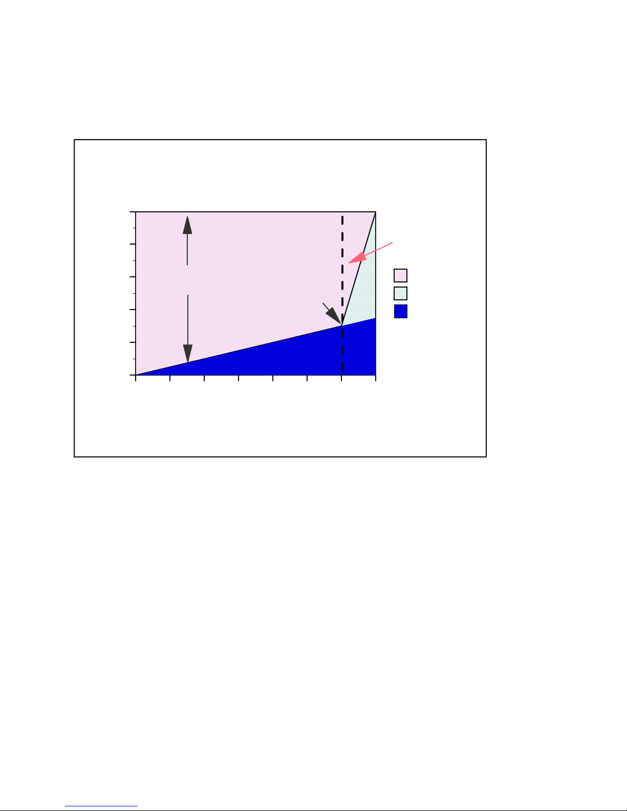
Model 7xx and 9/98 Model 170 CPU

CPU Distribution vs. Interactive Utilization

100

Announced Capacities Stop Here!

Available for Client/Server

Available CPU %

Knee

available overhead interactive

0 Full7/6

Fraction of Interactive CPW

Applies to: Model 170 anno un ce d in 9/98 and ALL systems announce d o n or after 2/99

Figure 2.1. Server Model behavior

The figure above shows a straight line for the effective interactive utilization. Real/customer environments will produce a curved line since most environments will be dynamic, due to job initiation, interrupts, etc.

In general, a single interactive job will not cause a significant impact to client/server performance

Microcode task CFINTn, for all iSeries models, handles interrupts, task switching, and other similar system overhead functions. For the server models, when interactive processing exceeds a threshold amount, the additional overhead required will be manifest in the CFINTn task. Note that a single interactive job will not incur this overhead.

There is one CFINTn task for each processor. For example, on a single processor system only CFINT1 will appear. On an 8-way processor, system tasks CFINT1 through CFINT8 will appear. It is possible to see significant CFINT activity even when server/interactive overhead does not exist. For example if there are lots of synchronous or communication I/O or many jobs with many task switches.

The effective interactive utilization (EIU) for a server system can be defined as the useable interactive utilization plus the total of CFINT utilization.

IBM i 6.1 Performance Capabilities Reference - January/April/October 2008

2.3 Server Model Differences

Server models were designed for a client/server workload and to accommodate an interactive workload. When the interactive workload exceeds an interactive CPW threshold (the “knee of the curve”) the client/server processing performance of the system becomes increasingly impacted at an accelerating rate beyond the knee as interactive workload continues to build. Once the interactive workload reaches the maximum interactive CPW value, all the CPU cycles are being used and there is no capacity available for handling client/server tasks.

Custom server models interact with batch and interactive workloads similar to the server models but the degree of interaction and priority of workloads follows a different algorithm and hence the knee of the curve for workload interaction is at a different point which offers a much higher interactive workload capability compared to the standard server models.

For the server models the knee of the curve is approximately:

y 100% of interactive CPW for:

y iSeries model 170s announced on or after 9/98 y 7xx models

y 6/7 (86%) of interactive CPW for:

y AS/400e custom servers

y 1/3 of interactive CPW for:

y AS/400 Advanced Servers y AS/400e servers y AS/400e model 150 y iSeries model 170s announced in 2/98

For the 7xx models the interactive capacity is a feature that can be sized and purchased like any other feature of the system (i.e. disk, memory, communication lines, etc.).

The following charts show the CPU distribution vs. interactive utilization for Custom Server and pre-2/99 Server models.

IBM i 6.1 Performance Capabilities Reference - January/April/October 2008

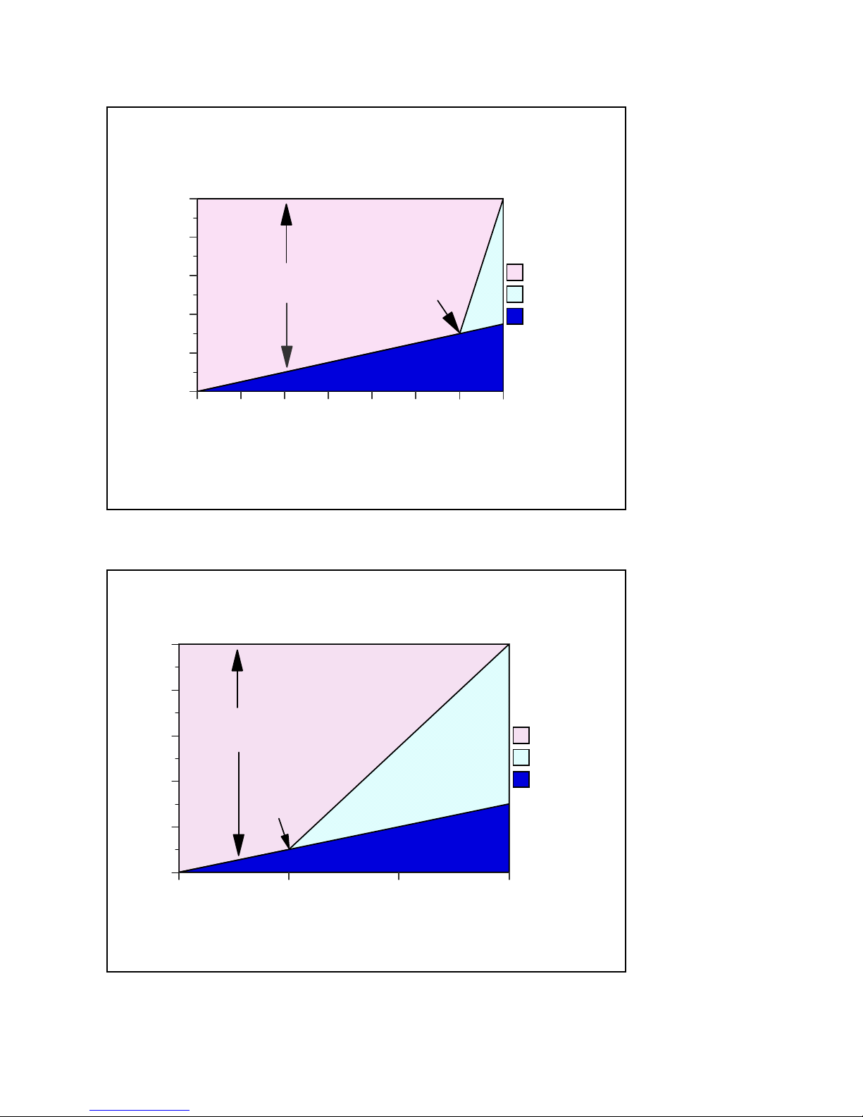
Custom Server Model

CPU Distribution vs. Interactive Utilization

100

Available for Client/Server

Knee

Available CPU

0 6/7 Full

Fraction of Interactive CPW

Applies to: AS/400e Custom Servers, AS/400e Mixed Mode Servers

Figure 2.2. Custom Server Model behavior

available CFINT interactive

Server Model

CPU Distribution vs. Interactive Utilization

100

Available for

Available CPU

Figure 2.3. Server Model behavior

Client/Server

0 1/3 Int-CPW Full Int-CPW

Fraction of Interactive CPW

Applies to: AS/400 Advanced Servers, AS/400e servers,

Model 150, Model 170s announced in 2/98

Knee

available CFINT interactive

IBM i 6.1 Performance Capabilities Reference - January/April/October 2008

2.4 Performance Highlights of Model 7xx Servers

7xx models were designed to accommodate a mixture of traditional “green screen” applications and more intensive “server” environments. Interactive features may be upgraded if additional interactive capacity is required. This is similar to disk, memory, or other features.

Each system is rated with a processor CPW which represents the relative performance (maximum capacity) of a processor feature running a commercial processing workload (CPW) in a client/server environment. Processor CPW is achievable when the commercial workload is not constrained by main storage or DASD.

Each system may have one of several interactive features. Each interactive feature has an interactive CPW associated with it. Interactive CPW represents the relative performance available to perform host-centric (5250) workloads. The amount of interactive capacity consumed will reduce the available processor capacity by the same amount. The following example will illustrate this performance capacity interplay:

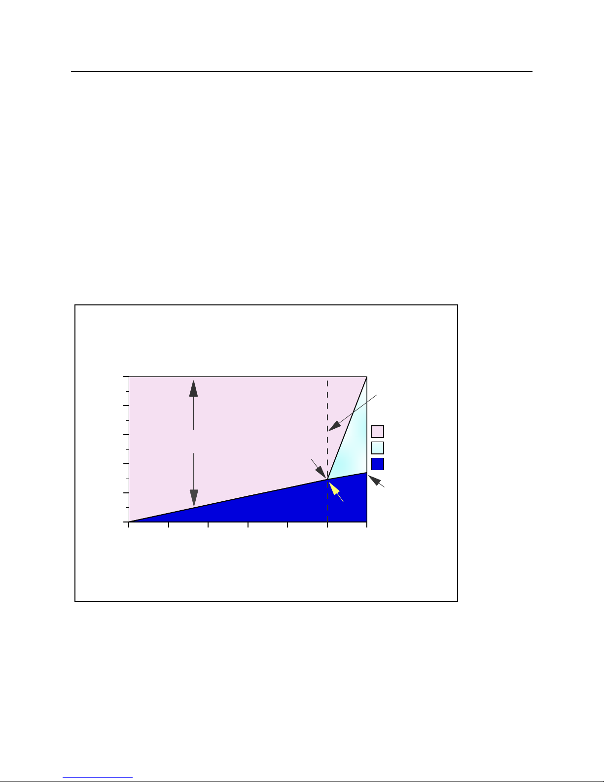
Model 7xx and 9/98 Model 170

CPU Distribution vs. Interactive Utilization

Model 7xx Processor FC 206B (240 / 70 CPW)

100

Available for Client/Server

Available CPU %

Knee

29.2%

Announced Capacities Stop Here!

available CFINT interactive

34%

0 20 40 60 80 100 117

% of Published Interactive CPU

Applies to: Mo del 170 announced in 9/98 and ALL systems announced on or after 2/99

Figure 2.4. Model 7xx Utilization Example

(7/6)

At 110% of percent of the published interactive CPU, or 32.1% of total CPU, CFINT will use an additional 39.8% (approximate) of the total CPU, yielding an effective interactive CPU utilization of approximately 71.9%. This leaves approximately 28.1% of the total CPU available for client/server work. Note that the CPU is completely utilized once the interactive workload reaches about 34%. (CFINT would use approximately 66% CPU). At this saturation point, there is no CPU available for client/server.

IBM i 6.1 Performance Capabilities Reference - January/April/October 2008

2.5 Performance Highlights of Model 170 Servers

iSeries Dedicated Server for Domino models will be generally available on September 24, 1999. Please refer to Section 2.13, iSeries Dedicated Server for Domino Performance Behavior, for additional

information.

Model 170 servers (features 2289, 2290, 2291, 2292, 2385, 2386 and 2388) are significantly more powerful than the previous Model 170s announced in Feb. '98. They have a faster processor (262MHz vs. 125MHz) and more main memory (up to 3.5GB vs. 1.0GB). In addition, the interactive workload balancing algorithm has been improved to provide a linear relationship between the client/server (batch) and published interactive workloads as measured by CPW.

The CPW rating for the maximum client/server workload now reflects the relative processor capacity rather than the "system capacity" and therefore there is no need to state a "constrained performance" CPW. This is because some workloads will be able to run at processor capacity if they are not DASD, memory, or otherwise limited.

Just like the model 7xx, the current model 170s have a processor capacity (CPW) value and an interactive capacity (CPW) value. These values behave in the same manner as described in the Performance highlights of new model 7xx servers section.

As interactive workload is added to the current model 170 servers, the remaining available client/server (batch) capacity available is calculated as: CPW (C/S batch) = CPW(processor) - CPW(interactive) This is valid up to the published interactive CPW rating. As long as the interactive CPW workload does not exceed the published interactive value, then interactive performance and client/server (batch) workloads will be both be optimized for best performance. Bottom line, customers can use the entire

interactive capacity with no impacts to client/server (batch) workload response times.

On the current model 170s, if the published interactive capacity is exceeded, system overhead grows very quickly, and the client/server (batch) capacity is quickly reduced and becomes zero once the interactive workload reaches 7/6 of the published interactive CPW for that model.

The absolute limit for dedicated interactive capacity on the current models can be computed by multiplying the published interactive CPW rating by a factor of 7/6. The absolute limit for dedicated client/server (batch) is the published processor capacity value. This assumes that sufficient disk and memory as well as other system resources are available to fit the needs of the customer's programs, etc. Customer workloads that would require more than 10 disk arms for optimum performance should not be expected to give optimum performance on the model 170, as 10 disk access arms is the maximum configuration. When the model 170 servers are running less than the published interactive workload, no Server Dynamic Tuning (SDT) is necessary to achieve balanced performance between interactive and client/server (batch) workloads. However, as with previous server models, a system value (QDYNPTYADJ - Server Dynamic Tuning ) is available to determine how the server will react to work requests when interactive workload exceeds the "knee". If the QDYNPTYADJ value is turned on, client/server work is favored over additional interactive work. If it is turned off, additional interactive work is allowed at the expense of low-priority client/server work. QDYNPTYADJ only affects the server when interactive requirements exceed the published interactive capacity rating. The shipped default value is for QDYNPTYADJ to be turned on.

IBM i 6.1 Performance Capabilities Reference - January/April/October 2008

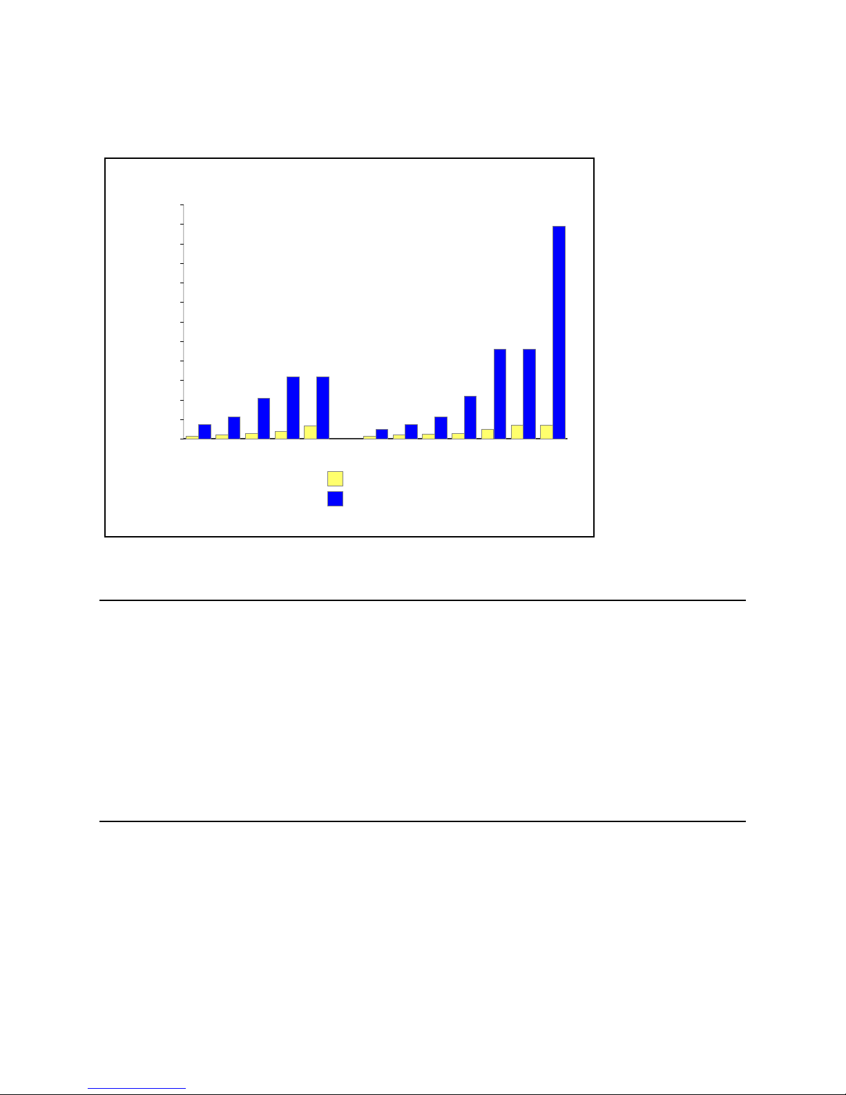
The next chart shows the performance capacity of the current and previous Model 170 servers.

Previous vs. Current AS/400e server 170 Performance

1200

1090

1000

800

600

400

CPW Values

200

114

2159 2160 2164 2176 2183 2289 2290 2291 2292 2385 2386 2388

Previous *

319 319

210

Current

460 460

220

115

70 70

Interactive Processor

* Unconstrained V4R2 rates

Figure 2.5. Previous vs. Current Server 170 Performance

2.6 Performance Highlights of Custom Server Models

Custom server models were available in releases V4R1 through V4R3. They interact with batch and interactive workloads similar to the server models but the degree of interaction and priority of workloads is different, and the knee of the curve for workload interaction is at a different point. When the interactive workload exceeds approximately 6/7 of the maximum interactive CPW (the knee of the curve), the client/server processing performance of the system becomes increasingly impacted. Once the interactive workload reaches the maximum interactive CPW value, all the CPU cycles are being used and there is no capacity available for handling client/server tasks.

2.7 Additional Server Considerations

It is recommended that the System Operator job run at runpty(9) or less. This is because the possibility exists that runaway interactive jobs will force server/interactive overhead to their maximum. At this point it is difficult to initiate a new job and one would need to be able to work with jobs to hold or cancel runaway jobs.

You should monitor the interactive activity closely. To do this take advantage of PM/400 or else run Collection Services nearly continuously and query monitor data base each day for high interactive use

IBM i 6.1 Performance Capabilities Reference - January/April/October 2008

and higher than normal CFINT values. The goal is to avoid exceeding the threshold (knee of the curve) value of interactive capacity.

2.8 Interactive Utilization

When the interactive CPW utilization is beyond the knee of the curve, the following formulas can be used to determine the effective interactive utilization or the available/remaining client/server CPW. These

equations apply to all server models.

CPWcs(maximum) = client/server CPW maximum value CPWint(maximum) = interactive CPW maximum value CPWint(knee) = interactive CPW at the knee of the curve CPWint = interactive CPW of the workload

X is the ratio that says how far into the overhead zone the workload has extended: X = (CPWint - CPWint(knee)) / (CPWint(maximum) - CPWint(knee))

EIU = Effective interactive utilization. In other words, the free running, CPWint(knee), interactive plus the combination of interactive and overhead generated by X. EIU = CPWint(knee) + (X * (CPWcs(maximum) - CPWint(knee)))

CPW remaining for batch = CPWcs(maximum) - EIU

Example 1:

A model 7xx server has a Processor CPW of 240 and an Interactive CPW of 70. The interactive CPU percent at the knee equals (70 CPW / 240 CPW) or 29.2%. The maximum interactive CPU percent (7/6 of the Interactive CPW ) equals (81.7 CPW / 240 CPW) or 34%.

Now if the interactive CPU is held to less than 29.2% CPU (the knee), then the CPU available for the System, Batch, and Client/Server work is 100% - the Interactive CPU used.

If the interactive CPU is allowed to grow above the knee, say for example 32.1 % (110% of the knee), then the CPU percent remaining for the Batch and System is calculated using the formulas above:

X = (32.1 - 29.2) / (34 - 29.2) = .604 EIU = 29.2 + (.604 * (100 - 29.2)) = 71.9%

CPW remaining for batch = 100 - 71.9 = 28.1%

Note that a swing of + or - 1% interactive CPU yields a swing of effective interactive utilization (EIU) from 57% to 87%. Also note that on custom servers and 7xx models, environments that go beyond the interactive knee may experience erratic behavior.

Example 2:

A Server Model has a Client/Server CPW of 450 and an Interactive CPW of 50. The maximum interactive CPU percent equals (50 CPW / 450 CPW) or 11%. The interactive CPU percent at the knee is 1/3 the maximum interactive value. This would equal 4%.

IBM i 6.1 Performance Capabilities Reference - January/April/October 2008

Now if the interactive CPU is held to less than 4% CPU (the knee), then the CPU available for the System, Batch, and Client/Server work is 100% - the Interactive CPU used.

If the interactive CPU is allowed to grow above the knee, say for example 9% (or 41 CPW), then the CPU percent remaining for the Batch and System is calculated using the formulas above:

X = (9 - 4) / (11 - 4) = .71 (percent into the overhead area) EIU = 4 + (.71 * (100 - 4)) = 72%

CPW remaining for batch = 100 - 72 = 28%

Note that a swing of + or - 1% interactive CPU yields a swing of effective interactive utilization (EIU) from 58% to 86%.

On earlier server models, the dynamics of the interactive workload beyond the knee is not as abrupt, but because there is typically less relative interactive capacity the overhead can still cause inconsistency in response times.

2.9 Server Dynamic Tuning (SDT)

Logic was added in V4R1 and is still in use today so customers could better control the impact of interactive work on their client/server performance. Note that with the new Model 170 servers (features 2289, 2290, 2291, 2292, 2385, 2386 and 2388) this logic only affects the server when interactive requirements exceed the published interactive capacity rating. For further details see the section, Performance highlights of current model 170 servers.

Through dynamic prioritization, all interactive jobs will be put lower in the priority queue, approximately at the knee of the curve. Placing the interactive jobs at a lesser priority causes the interactive jobs to slow down, and more processing power to be allocated to the client/server processing. As the interactive jobs receive less processing time, their impact on client/server processing will be lessened. When the interactive jobs are no longer impacting client/server jobs, their priority will dynamically be raised again.

The dynamic prioritization acts as a regulator which can help reduce the impact to client/server processing when additional interactive workload is placed on the system. In most cases, this results in better overall throughput when operating in a mixed client/server and interactive environment, but it can cause a noticeable slowdown in interactive response.

To fully enable SDT, customers MUST use a non-interactive job run priority (RUNPTY parameter) value of 35 or less (which raises the priority, closer to the default priority of 20 for interactive jobs).

Changing the existing non-interactive job’s run priority can be done either through the Change Job (CHGJOB) command or by changing the RUNPTY value of the Class Description object used by the non-interactive job. This includes IBM-supplied or application provided class descriptions.

Examples of IBM-supplied class descriptions with a run priority value higher than 35 include QBATCH and QSNADS and QSYSCLS50. Customers should consider changing the RUNPTY value for QBATCH and QSNADS class descriptions or changing subsystem routing entries to not use class descriptions QBATCH, QSNADS, or QSYSCLS50.

IBM i 6.1 Performance Capabilities Reference - January/April/October 2008

If customers modify an IBM-supplied class description, they are responsible for ensuring the priority value is 35 or less after each new release or cumulative PTF package has been installed. One way to do this is to include the Change Class (CHGCLS) command in the system Start Up program.

NOTE: Several IBM-supplied class descriptions already have RUNPTY values of 35 or less. In these cases no user action is required. One example of this is class description QPWFSERVER with RUNPTY(20). This class description is used by Client Access database server jobs QZDAINIT (APPC) and QZDASOINIT (TCP/IP).

The system deprioritizes jobs according to groups or "bands" of RUNPTY values. For example, 10-16 is band 1, 17-22 is band 2, 23-35 is band 3, and so on.

Interactive jobs with priorities 10-16 are an exception case with V4R1. Their priorities will not be adjusted by SDT. These jobs will always run at their specified 10-16 priority.

When only a single interactive job is running, it will not be dynamically reprioritized.

When the interactive workload exceeds the knee of the curve, the priority of all interactive jobs is decreased one priority band, as defined by the Dynamic Priority Scheduler, every 15 seconds. If needed, the priority will be decreased to the 52-89 band. Then, if/when the interactive CPW work load falls below the knee, each interactive job's priority will gradually be reset to its starting value when the job is dispatched.

If the priority of non-interactive jobs are not set to 35 or lower, SDT stills works, but its effectiveness is greatly reduced, resulting in server behavior more like V3R6 and V3R7. That is, once the knee is exceeded, interactive priority is automatically decreased. Assuming non-interactive is set at priority 50, interactive could eventually get decreased to the 52-89 priority band. At this point, the processor is slowed and interactive and non-interactive are running at about the same priority. (There is little priority difference between 47-51 band and the 52-89 band.) If the Dynamic Priority Scheduler is turned off, SDT is also turned off.

Note that even with SDT, the underlying server behavior is unchanged. Customers get no more CPU cycles for either interactive or non-interactive jobs. SDT simply tries to regulate interactive jobs once they exceed the knee of the curve.

Obviously systems can still easily exceed the knee and stay above it, by having a large number of interactive jobs, by setting the priority of interactive jobs in the 10-16 range, by having a small client/server workload with a modest interactive workload, etc. The entire server behavior is a partnership with customers to give non-interactive jobs the bulk of the CPU while not entirely shutting out interactive.

To enable the Server Dynamic Tuning enhancement ensure the following system values are on: (the shipped defaults are that they are set on)

y QDYNPTYSCD - this improves the job scheduling based on job impact on the system. y QDYNPTYADJ - this uses the scheduling tool to shift interactive priorities after the threshold is

reached.

The Server Dynamic Tuning enhancement is most effective if the batch and client/server priorities are in the range of 20 to 35.

IBM i 6.1 Performance Capabilities Reference - January/April/October 2008

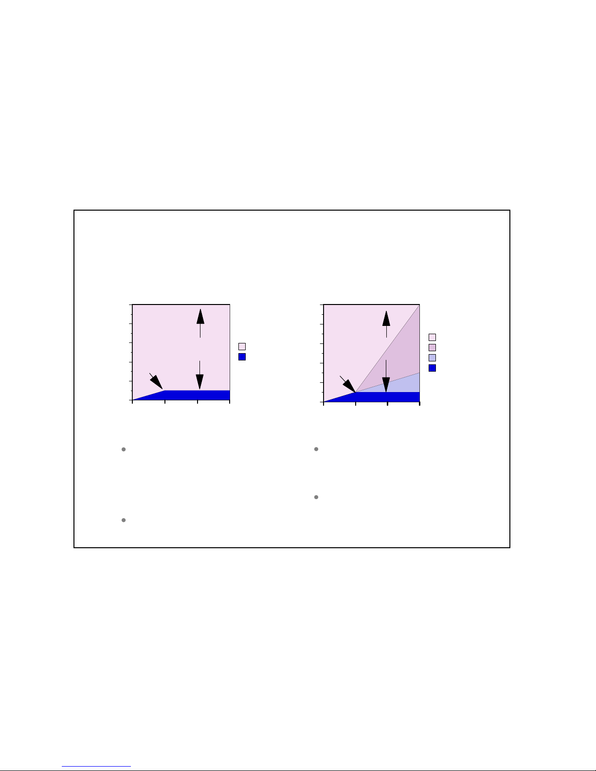
Server Dynamic Tuning Recommendations

On the new systems and mixed mode servers have the QDYNPTYSCD and QDYNPTYADJ system value set on. This preserves non-interactive capacities and the interactive response times will be dynamic beyond the knee regardless of the setting. Also set non-interactive class run priorities to less than 35.

On earlier servers and 2/98 model 170 systems use your interactive requirements to determine the settings. For “pure interactive” environments turn the QDYNPTYADJ system value off. in mixed environments with important non-interactive work, leave the values on and change the run priority of important non-interactive work to be less than 35.

Affects of Server Dynamic Tuning

Server Dynamic Tuning - .

High "Server" Demand

100

Knee

Available CPU

0 1/3 Int-CPW Full Int-CPW

Fraction of Interactive CPW

With sufficient batch or client/server load, Interactive is constrained to the "knee-level" by priority degradation

Interactive suffers poor response times

Available for Client/Server

available interactive

Server Dynamic Tuning

Mixed "Server" Demand

100

Knee

Available CPU

0 1/3 Int-CPW Full Int-CPW

Fraction of Interactive CPW

Without high "server" demand, Interactive allowed to grow to limit

Overhead introduced just as when Dynamic Priority Adjust is turned off

Available for Client/Server

available O.H. or Server Int. or Server interactive

Figure 2.6.

IBM i 6.1 Performance Capabilities Reference - January/April/October 2008

2.10 Managing Interactive Capacity

Interactive/Server characteristics in the real world.

Graphs and formulas listed thus far work perfectly, provided the workload on the system is highly regular and steady in nature. Of course, very few systems have workloads like that. The more typical case is a dynamic combination of transaction types, user activity, and batch activity. There may very well be cases where the interactive activity exceeds the documented limits of the interactive capacity, yet decreases quickly enough so as not to seriously affect the response times for the rest of the workload. On the other hand, there may also be some intense transactions that force the interactive activity to exceed the documented limits interactive feature for a period of time even though the average CPU utilization appears to be less than these documented limits.

For 7xx systems, current 170 systems, and mixed-mode servers, a goal should be set to only rarely exceed the threshold value for interactive utilization. This will deliver the most consistent performance for both interactive and non-interactive work.

The questions that need to be answered are:

1. “How do I know whether my system is approaching the interactive limits or not?”

2. “What is viewed as ‘interactive’ by the system?”

3. “How close to the threshold can a system get without disrupting performance?”

This section attempts to answer these questions.

Observing Interactive CPU utilization

The most commonly available method for observing interactive utilization is Collection Services used in conjunction with the Performance Tools program product. The monitor collects system data as well as data for each job on the system, including the CPU consumed and the type of job. By examining the reports generated by the Performance Tools product, or by writing a query against the data in the various performance data base files.

Note: data is written to these files based on sample interval (Smallest is 5 minutes, default is 15 minutes). This data is an average for the duration of a measurement interval.

1. The first metric of interest is how much of the system’s interactive capacity has been used. The file

QAPMSYSCPU field SCIFUS contains the amount of interactive feature CPU time used. This metric became available with Collection Services in V4R5.

2. Even though average CPU may be reasonable your interactive workload may still be exceeding limits

at times. The file QAPMSYSCPU field SCIFTE contains the amount of time the interactive threshold was exceeded during the interval. This metric became available with Collection Services in V4R5.

3. To determine what jobs are responsible for interactive feature consumption, you can look at the data

in QAPMJOBL (Collection Services) or QAPMJOBS (Performance Monitor): y If using Collection Services on a V5R1 or later system, those jobs which the machine considers to

be interactive are indicated by the field JBSVIF =’1’. These are all jobs that could contribute to your interactive feature utilization.

y In all cases you can examine the jobs that are considered interactive by OS/400 as indicated by

field JBTYPE = “I”. Although not totally accurate, in most cases this will provide an adequate list of jobs that contributed to interactive utilization.

IBM i 6.1 Performance Capabilities Reference - January/April/October 2008

There are other means for determining interactive utilization. The easiest of these is the performance monitoring function of Management Central, which became available with V4R3. Management Central can provide:

y Graphical, real-time monitoring of interactive CPU utilization y Creation of an alert threshold when an alert feature is turned on and the graph is highlighted y Creation of an reverse threshold below which the highlights are turned off y Multiple methods of handling the alert, from a console message to the execution of a command to the

forwarding of the alert to another system.

By taking the ratio of the Interactive CPW rating and the Processor CPW rating for a system, one can determine at what CPU percentage the threshold is reached (This ratio works for the 7xx models and the current model 170 systems. For earlier models, refer to other sections of this document to determine what fraction of the Interactive CPW rating to use.) Depending on the workload, an alert can be set at some percentage of this level to send a warning that it may be time to redistribute the workload or to consider upgrading the interactive feature.

Finally, the functions of PM400 can also show the same type of data that Collection Services shows, with the advantage of maintaining a historical view, and the disadvantage of being only historical. However, signing up for the PM400 service can yield a benefit in determining the trends of how interactive capacities are used on the system and whether more capacity may be needed in the future.

Is Interactive really Interactive?

Earlier in this document, the types of jobs that are classified as interactive were listed. In general, these jobs all have the characteristic that they have a 5250 workstation communications path somewhere within the job. It may be a 5250 data stream that is translated into html, or sent to a PC for graphical display, but the work on the iSeries is fundamentally the same as if it were communicating with a real 5250-type display. However, there are cases where jobs of type “I” may be charged with a significant amount of work that is not “interactive”. Some examples follow:

y Job initialization: If a substantial amount of processing is done by an interactive job’s initial program,

prior to actually sending and receiving a display screen as a part of the job, that processing may not be included as a part of the interactive work on the system. However, this may be somewhat rare, since most interactive jobs will not have long-running initial programs.

y More common will be parallel activities that are done on behalf of an interactive job but are not done

within the job. There are two database-related activities where this may be the case.

1. If the QQRYDEGREE system value is adjusted to allow for parallelism or the CHGQRYA command is used to adjust it for a single job, queries may be run in service jobs which are not interactive in nature, and which do not affect the total interactive utilization of the system. However, the work done by these service jobs is charged back to the interactive job. In this case, Collection Services and most other mechanisms will all show a higher sum of interactive CPU utilization than actually occurs. The exception to this is the WRKSYSACT command, which may show the current activity for the service jobs and/or the activity that they have “charged back” to the requesting jobs. Thus, in this situation it is possible for WRKSYSACT to show a lower system CPU utilization than the sum of the CPU consumption for all the jobs.

IBM i 6.1 Performance Capabilities Reference - January/April/October 2008

2. A similar effect can be found with index builds. If parallelism is enabled, index creation (CRTLF, Create Index, Open a file with MAINT(*REBUILD), or running a query that requires an index to be build) will be sent to service jobs that operate in non-interactive mode, but charge their work back to the job that requested the service. Again, the work does not count as “interactive”, but the performance data will show the resource consumption as if they were.

y Lastly when only a single interactive job is running, the machine grants an exemption and does not

include this job’s activity in the interactive feature utilization.

There are two key ideas in the statements above. First, if the workload has a significant component that is related to queries or there is a single interactive job running, it will be possible to show an interactive job utilization in the performance tools that is significantly higher than what would be assumed and reported from the ratings of the Interactive Feature and the Processor Feature. Second, although it may make monitoring interactive utilization slightly more difficult, in the case where the workload has a significant query component, it may be beneficial to set the QQRYDEGREE system value to allow at least 2 processes, so that index builds and many queries can be run in non-interactive mode. Of course, if the nature of the query is such that it cannot be split into multiple tasks, the whole query is run inside the interactive job, regardless of how the system value is set.

How close to the threshold can a system get without disrupting performance?

The answer depends on the dynamics of the workload, the percentage of work that is in queries, and the projected growth rate. It also may depend on the number of processors and the overall capacity of the interactive feature installed. For example, a job that absorbs a substantial amount of interactive CPU on a uniprocessor may easily exceed the threshold, even though the “normal” work on the system is well under it. On the other hand, the same job on a 12-way can use at most 1/12th of the CPU, or 8.3%. a single, intense transaction may exceed the limit for a short duration on a small system without adverse affects, but on a larger system the chances of having multiple intense transactions may be greater.

With all these possibilities, how much of the Interactive feature can be used safely? A good starting point is to keep the average utilization below about 70% of the threshold value (Use double the threshold value for the servers and earlier Model 170 systems that use the 1/3 algorithm described earlier in this document.) If the measurement mechanism averages the utilization over a 15 minute or longer period, or if the workload has a lot of peaks and valleys, it might be worthwhile to choose a target that is lower than 70%. If the measurement mechanism is closer to real-time, such as with Management Central, and if the workload is relatively constant, it may be possible to safely go above this mark. Also, with large interactive features on fairly large processors, it may be possible to safely go to a higher point, because the introduction of workload dynamics will have a smaller effect on more powerful systems.

As with any capacity-related feature, the best answer will be to regularly monitor the activity on the system and watch for trends that may require an upgrade in the future. If the workload averages 60% of the interactive feature with almost no overhead, but when observed at 65% of the feature capacity it shows some limited amount of overhead, that is a clear indication that a feature upgrade may be required. This will be confirmed as the workload grows to a higher value, but the proof point will be in having the historical data to show the trend of the workload.

IBM i 6.1 Performance Capabilities Reference - January/April/October 2008

2.11 Migration from Traditional Models

This section describes a suggested methodology to determine which server model is appropriate to contain the interactive workload of a traditional model when a migration of a workload is occurring. It is assumed that the server model will have both interactive and client/server workloads.

To get the same performance and response time, from a CPU perspective, the interactive CPU utilization of the current traditional model must be known. Traditional CPU utilization can be determined in a number of ways. One way is to sum up the CPU utilization for interactive jobs shown on the Work with Active Jobs (WRKACTJOB) command.

*************************************************************************** Work with Active Jobs

CPU %: 33.0 Elapsed time: 00:00:00 Active jobs: 152

Type options, press Enter.

2=Change 3=Hold 4=End 5=Work with 6=Release 7=Display message 8=Work with spooled files 13=Disconnect ...

Opt Subsystem/Job User Type CPU % Function Status __ BATCH QSYS SBS 0 DEQW __ QCMN QSYS SBS 0 DEQW __ QCTL QSYS SBS 0 DEQW __ QSYSSCD QPGMR BCH 0 PGM-QEZSCNEP EVTW __ QINTER QSYS SBS 0 DEQW __ DSP05 TESTER INT 0.2 PGM-BUPMENUNE DSPW __ QPADEV0021 TEST01 INT 0.7 CMD-WRKACTJOB RUN __ QSERVER QSYS SBS 0 DEQW __ QPWFSERVSD QUSER BCH 0 SELW __ QPWFSERVS0 QUSER PJ 0 DEQW **************************************************************************

(Calculate the average of the CPU utilization for all job types "INT" for the desired time interval for interactive CPU utilization - "P" in the formula shown below.)

Another method is to run Collection Services during selected time periods and review the first page of the Performance Tools for iSeries licensed program Component Report. The following is an example of this section of the report:

IBM i 6.1 Performance Capabilities Reference - January/April/October 2008

*********************************************************************************** Component Report

Component Interval Activity

Data collected 190396 at 1030

Member . . . : Q960791030 Model/Serial . : 310-2043/10-0751D Main St... Library. . : PFR System name. . : TEST01 Version/Re..

CPU %

Batch

Disk I/O

per sec

Sync

Disk I/O

per sec

Async

39102.946.332.285.20.86,16410:36

33.9103.339.545.291.30.97,40410:41

33.296.65138.897.60.75,46610:46

4986.657.435.697.91.25,62210:51

40.764.277.416.597.90.84,52710:56

19.956.525.774.299.91.85,06811:51

32.665.545.546.899.92.45,99111:56

End

Rsp/TnsTns/hrITV

CPU %

Total

CPU%

Inter

Itv End------Interval end time (hour and minute) Tns/hr-------Number of interactive transactions per hour Rsp/Tns-----Average interactive transaction response time

*********************************************************************************** (Calculate the average of the CPU utilization under the "Inter" heading for the desired time interval for interactive CPU utilization - "P" in the formula shown below.)

It is possible to have interactive jobs that do not show up with type "INT" in Collection Services or the Component Report. An example is a job that is submitted as a batch job that acquires a work station. These jobs should be included in the interactive CPU utilization count.

Most systems have peak workload environments. Care must be taken to ensure that peaks can be contained in server model environments. Some environments could have peak workloads that exceed

the interactive capacity of a server model or could cause unacceptable response times and throughput.

In the following equations, let the interactive CPU utilization of the existing traditional system be represented by percent P. A server model that should then produce the same response time and throughput would have a CPW of: Server Interactive CPW = 3 * P * Traditional CPW or for Custom Models use: Server Interactive CPW = 1.0 * P * Traditional CPW (when P < 85%) or Server interactive CPW = 1.5 * P * Traditional CPW (when P >= 85%)

Use the 1.5 factor to ensure the custom server is sized less than 85% CPU utilization.

These equations provide the server interactive CPU cycles required to keep the interactive utilization at or below the knee of the curve, with the current interactive workload. The equations given at the end of the Server and Custom Server Model Behavior section can be used to determine the effective interactive utilization above the knee of the curve. The interactive workload below the knee of the curve represents

IBM i 6.1 Performance Capabilities Reference - January/April/October 2008

one third of the total possible interactive workload, for non-custom models. The equation shown in this section will migrate a traditional system to a server system and keep the interactive workload at or below the knee of the curve, that is, using less than two thirds of the total possible interactive workload. In some environments these equations will be too conservative. A value of 1.2, rather than 1.5 would be less conservative. The equations presented in the Interactive Utilization section should be used by those customers who understand how server models work above the knee of the curve and the ramifications of the V4R1 enhancement.

These equations are for migration of “existing workload” situations only. Installation workload projections for “initial installation” of new custom servers are generally sized by the business partner for 50 - 60% CPW workloads and no “formula increase” would be needed.

For example, assume a model 510-2143 with a single V3R6 CPW rating of 66.7 and assume the Performance Tools for iSeries report lists interactive work CPU utilization as 21%. Using the previous formula, the server model must have an interactive CPW rating of at least 42 to maintain the same performance as the 510-2143.

Server interactive CPW = 3 * P * Traditional CPW = 3 * .21 * 66.7 = 42

A server model with an interactive CPW rating of at least 42 could approximate the same interactive work of the 510-2143, and still leave system capacity available for client/server activity. An S20-2165 is the first AS/400e series with an acceptable CPW rating (49.7).

Note that interactive and client/server CPWs are not additive. Interactive workloads which exceed (even briefly) the knee of the curve will consume a disproportionate share of the processing power and may result in insufficient system capacity for client/server activity and/or a significant increase in interactive response times.

2.12 Upgrade Considerations for Interactive Capacity

When upgrading a system to obtain more processor capacity, it is important to consider upgrading the interactive capacity, even if additional interactive work is not planned. Consider the following hypothetical example:

y The original system has a processor capacity of 1000 CPW and an interactive capacity of 250 ICPW y The proposed upgrade system has a processor capacity of 4000 CPW and also offers an interactive

capacity of 250 ICPW.

y On the original system, the interactive capacity allowed 25% of the total system to be used for

interactive work. On the new system, the same interactive capacity only allows 6.25% of the total system to be used for interactive work.

y Even though the total interactive capacity of the system has not changed, the faster processors (and

likely larger memory and faster disks) will allow interactive requests to complete more rapidly, which can cause greater spikes of interactive demand.

y So, just as it is important to consider balancing memory and disk upgrades with processor upgrades,

optimal performance may also require an interactive capacity upgrade when moving to a new system.

IBM i 6.1 Performance Capabilities Reference - January/April/October 2008

2.13 iSeries for Domino and Dedicated Server for Domino Performance Behavior

In preparation for future Domino releases which will provides support for DB2 files, the previous processing limitations associated with DSD models have been removed in i5/OS V5R3.

In addition, a PTF is available for V5R2 which also removes the processing limitations for DSD models and allows full use of DB2. Please refer to PTF MF32968 and its prerequisite requirements.

The sections below from previous versions of this document are provided for those users on OS/400 releases prior to V5R3.

2.13.1 V5R2 iSeries for Domino & DSD Performance Behavior updates

Included in the V5R2 February 2003 iSeries models are five iSeries for Domino offerings. These include three i810 and two i825 models. The iSeries for Domino offerings are specially priced and configured for Domino workloads. There are no processing guidelines for the iSeries for Domino offerings as with non-Domino processing on the Dedicated Server for Domino models. With the iSeries for Domino offerings the full amount of DB2 processing is available, and it is no longer necessary to have Domino processing active for non-Domino applications to run well. Please refer to Chapter 11 for additional information on Domino performance in iSeries, and Appendix C for information on performance specifications for iSeries servers.

For existing iSeries servers, OS/400 V5R2 (both the June 2002 and the updated February 2003 version) will exhibit similar performance behavior as V5R1 on the Dedicated Server for Domino models. The following discussion of the V5R1 Domino-complimentary behavior is applicable to V5R2.

Five new DSD models were announced with V5R1. These included the iSeries Model 270 with a 1-way and a 2-way feature, and the iSeries Model 820 with 1-way, 2-way, and 4-way features. In addition, OS/400 V5R1 was enhanced to bolster DSD server capacity for robust Domino applications that require Java Servlet and WebSphere Application Server integration. The new behavior which supports Domino-complementary workloads on the DSD was available after September 28, 2001 with a refreshed version of OS/400 V5R1. This enhanced behavior is applicable to all DSD models including the model 170 and previous 270 and 820 models. Additional information on Lotus Domino for iSeries can be found in Chapter 11, “Domino for iSeries”.

For information on the performance behavior of DSD models for releases prior to V5R1, please refer the to V4R5 version of this document.

Please refer to Appendix C for performance specifications for DSD models, including the number of Mail and Calendaring Users (MCU) supported.

2.13.2 V5R1 DSD Performance Behavior

This section describes the performance behavior for all DSD models for the refreshed version of OS/400 V5R1 that was available after September 28, 2001.

A white paper, Enhanced V5R1 Processing Capability for the iSeries Dedicated Server for Domino, provides additional information on DSD behavior and can be accessed at:

http://www.ibm.com/eserver/iseries/domino/pdf/dsdjavav5r1.pdf

IBM i 6.1 Performance Capabilities Reference - January/April/October 2008

Domino-Complementary Processing

Prior to V5R1, processing that did not spend the majority of its time in Domino code was considered non-Domino processing and was limited to approximately 10-15% of the system capacity. With V5R1, many applications that would previously have been treated as non-Domino may now be considered as Domino-complementary when they are used in conjunction with Domino. Domino-complementary processing is treated the same as Domino processing, provided it also meets the criteria that the DB2 processing is less than 15% CPU utilization as described below. This behavioral change has been made to support the evolving complexity of Domino applications which frequently require integration with function such as Java Servlets and WebSphere Application Server. The DSD models will continue to have a zero interactive CPW rating which allows sufficient capacity for systems management processing. Please see the section below on Interactive Processing.

In other words, non-Domino workloads are considered complementary when used simultaneously with Domino, provided they meet the DB2 processing criteria. With V5R1, the amount of DB2 processing on a DSD must be less than 15% CPU. The DB2 utilization is tracked on a system-wide basis and all applications on the DSD cumulatively should not exceed 15% CPU utilization. Should the 15% DB2 processing level be reached, the jobs and/or threads that are currently accessing DB2 resources may experience increased response times. Other processing will not be impacted.

Several techniques can used to determine and monitor the amount of DB2 processing on DSD (and non-DSD) iSeries servers for V4R5 and V5R1.

y Work with System Status (WRKSYSSTS) command, via the % DB capability statistic y Work with System Activity (WRKSYSACT) command

for iSeries, via the Overall DB CPU util statistic

which is part of the IBM Performance Tools

y Management Central - by starting a monitor to collect the CPU Utilization (Database Capability)

metric

y Workload section in the System Report which can be generated using the IBM Performance Tools for

iSeries, via the Total CPU Utilization (Database Capability) statistic

V5R1 Non-Domino Processing

Since all non-interactive processing is considered Domino-complementary when used simultaneously with Domino, provided it meets the DB2 criteria, non-Domino processing with V5R1 refers to the processing that is present on the system when there is no Domino processing present. (Interactive processing is a special case and is described in a separate section below). When there is no Domino processing present, all processing, including DB2 access, should be less than 10-15% of the system capacity. When the non-Domino processing capacity is reached, users may experience increased response times. In addition, CFINT processing may be present as the system attempts to manage the non-Domino processing to the available capacity. The announced “Processor CPW” for the DSD models refers to the amount of non-Domino processing that is supported .

Non-Domino processing on the 270 and 820 DSD models can be tracked using the Management Central function of Operations Navigator. Starting with V4R5, Management Central provides a special metric called “secondary utilization” which shows the amount of non-Domino processing. Even when Domino processing is present, the secondary utilization metric will include the Domino-complementary processing. And , as discussed above, the Domino-complementary processing running in conjunction with Domino will not be limited unless it exceeds the DB2 criteria.

Interactive Processing

IBM i 6.1 Performance Capabilities Reference - January/April/October 2008

Similar to previous DSD performance behavior for interactive processing, the Interactive CPW rating of 0 allows for system administrative functions to be performed by a single interactive user. In practice, a single interactive user will be able to perform necessary administrative functions without constraint. If multiple interactive users are simultaneously active on the DSD, the Interactive CPW capacity will likely be exceeded and the response times of those users may significantly lengthen. Even though the Interactive CPW capacity may be temporarily exceeded and the interactive users experience increased response times, other processing on the system will not be impacted. Interactive processing on the 270 and 820 DSD models can be tracked using the Management Central function of Operations Navigator.

Logical Partitioning on a Dedicated Server

With V5R1, iSeries logical partitioning is supported on both the Model 270 and Model 820. Just to be clear, iSeries logical partitioning is different from running multiple Domino partitions (servers). It is not necessary to use iSeries logical partitioning in order to be able to run multiple Domino servers on an iSeries system. iSeries logical partitioning lets you run multiple independent servers, each with its own processor, memory, and disk resources within a single symmetric multiprocessing iSeries. It also provides special capabilities such as having multiple versions of OS/400, multiple versions of Domino, different system names, languages, and time zone settings. For additional information on logical partitioning on the iSeries please refer to Chapter 18. Logical Partitioning (LPAR) and LPAR web at:

http://www.ibm.com/eserver/iseries/lpar

. When you use logical partitioning with a Dedicated Server, the DSD CPU processing guidelines are pro-rated for each logical partition based on how you divide up the CPU capability. For example, suppose you use iSeries logical partitioning to create two logical partitions, and specify that each logical partition should receive 50% of the CPU resource. From a DSD perspective, each logical partition runs independently from the other, so you will need to have Domino-based processing in each logical partition in order for non-Domino work to be treated as complementary processing. Other DSD processing requirements such as the 15% DB2 processing guidelines and the 15% non-Domino processing guideline will be divided between the logical partitions based on how the CPU was allocated to the logical partitions. In our example above with 50% of the CPU in each logical partition, the DB2 database guideline will be 7.5% CPU for each logical partition. Keep in mind that WRKSYSSTS and other tools show utilization only for the logical partition they are running in; so in our example of a partition that has been allocated 50% of the processor resource, a 7.5% system-wide load will be shown as 15% within that logical partition. The non-Domino processing guideline would be divided in a similar manner as the DB2 database guideline.

Running Linux on a Dedicated Server

As with other iSeries servers, to run Linux on a DSD it is necessary to use logical partitioning. Because Linux is it’s own unique operating environment and is not part of OS/400, Linux needs to have its own logical partition of system resources, separate from OS/400. The iSeries Hypervisor allows each partition to operate independently. When using logical partitioning on iSeries, the first logical partition, the primary partition, must be configured to run OS/400. For more information on running Linux on iSeries, please refer to Chapter 13. iSeries Linux Performance and Linux for iSeries web site at:

Http://www.ibm.com/eserver/iseries/linux

Running Linux in a DSD logical partition will exhibit different performance characteristics than running OS/400 in a DSD logical partition. As described in the section above, when running OS/400 in a DSD logical partition, the DSD capacities such as the 15% DB2 processing guideline and the 15% non-Domino processing guidelines are divided proportionately between the logical partitions based on how the processor resources were allocated to the logical partitions. However, for Linux logical partitions, the DSD guidelines are relaxed, and the Linux logical partition is able to use all of the resources allocated to it outside the normal guidelines for DSD processing. This means that it is not necessary to have Domino

IBM i 6.1 Performance Capabilities Reference - January/April/October 2008

processing present in the Linux logical partition, and all resources allocated to the Linux logical partition can essentially be used as though it were complementary processing. It is not necessary to proportionally increase the amount of Domino processing in the OS/400 logical partition to account for the fact that Domino processing is not present in the Linux logical partition .

By providing support for running Linux logical partitions on the Dedicated Server, it allows customers to run Linux-based applications, such as internet fire walls, to further enhance their Domino processing environment on iSeries. At the time of this publication, there is not a version of Domino that is supported for Linux logical partitions on iSeries.

IBM i 6.1 Performance Capabilities Reference - January/April/October 2008

Chapter 3. Batch Performance

In a commercial environment, batch workloads tend to be I/O intensive rather than CPU intensive. The factors that affect batch throughput for a given batch application include the following:

y Memory (Pool size) y CPU (processor speed) y DASD (number and type) y System tuning parameters

Batch Workload Description

The Batch Commercial Mix is a synthetic batch workload designed to represent multiple types of batch processing often associated with commercial data processing. The different variations allow testing of sequential vs random file access, changing the read to write ratio, generating "hot spots" in the data and running with expert cache on or off. It can also represent some jobs that run concurrently with interactive work where the work is submitted to batch because of a requirement for a large amount of disk I/O.

3.1 Effect of CPU Speed on Batch

The capacity available from the CPU affects the run time of batch applications. More capacity can be provided by either a CPU with a higher CPW value, or by having other contending applications on the same system consuming less CPU.

Conclusions/Recommendations

y For CPU-intensive batch applications, run time scales inversely with Relative Performance Rating

(CPWs). This assumes that the number synchronous disk I/Os are only a small factor.

y For I/O-intensive batch applications, run time may not decrease with a faster CPU. This is because

I/O subsystem time would make up the majority of the total run time.

y It is recommended that capacity planning for batch be done with tools that are available for iSeries.

For example, PATROL for iSeries - Predict from BMC Software, Inc. * (PID# 5620FIF) can be used for modeling batch growth and throughput. BATCH400 (an IBM internal tool) can be used for estimating batch run-time.

3.2 Effect of DASD Type on Batch

For batch applications that are I/O-intensive, the overall batch performance is very dependent on the speed of the I/O subsystem. Depending on the application characteristics, batch performance (run time) will be improved by having DASD that has:

y faster average service times y read ahead buffers y write caches

Additional information on DASD devices in a batch environment can be found in Chapter 14, “DASD Performance”.

IBM i 6.1 Performance Capabilities Reference - January/April/October 2008

3.3 Tuning Parameters for Batch

There are several system parameters that affect batch performance. The magnitude of the effect for each of them depends on the specific application and overall system characteristics. Some general information is provided here.

y Expert Cache

Expert Cache did not have a significant effect on the Commercial Mix batch workload. Expert Cache does not start to provide improvement unless the following are true for a given workload. These include:

y the application that is running is disk intensive, and disk I/O's are limiting the throughput. y the processor is under-utilized, at less than 60%. y the system must have sufficient main storage.

For Expert Cache to operate effectively, there must be spare CPU, so that when the average disk access time is reduced by caching in main storage, the CPU can process more work. In the Commercial Mix benchmark, the CPU was the limiting factor.

However, specific batch environments that are DASD I/O intensive, and process data sequentially may realize significant performance gains by taking advantage of larger memory sizes available on the RISC models, particularly at the high-end. Even though in general applications require more main storage on the RISC models, batch applications that process data sequentially may only require slightly more main storage on RISC. Therefore, with larger memory sizes in conjunction with using Expert Cache, these applications may achieve significant performance gains by decreasing the number of DASD I/O operations.

y Job Priority

Batch jobs can be given a priority value that will affect how much CPU processing time the job will get. For a system with high CPU utilization and a batch job with a low job priority, the batch throughput may be severely limited. Likewise, if the batch job has a high priority, the batch throughput may be high at the expense of interactive job performance.

y Dynamic Priority Scheduling

See 19.2, “Dynamic Priority Scheduling” for details.

y Application Techniques

The batch application can also be tuned for optimized performance. Some suggestions include: y Breaking the application into pieces and having multiple batch threads (jobs) operate concurrently.

Since batch jobs are typically serialized by I/O, this will decrease the overall required batch window requirements.

y Reduce the number of opens/closes, I/Os, etc. where possible.

y If you have a considerable amount of main storage available, consider using the Set Object Access

(SETOBJACC) command. This command pre-loads the complete database file, database index, or program into the assigned main storage pool if sufficient storage is available . The objective is to

IBM i 6.1 Performance Capabilities Reference - January/April/October 2008

improve performance by eliminating disk I/O operations.

y If communications lines are involved in the batch application, try to limit the number of

communications I/Os by doing fewer (and perhaps larger) larger application sends and receives. Consider blocking data in the application. Try to place the application on the same system as the frequently accessed data.

* BMC Software, the BMC Software logos and all other BMC Software products including PATROL for iSeries - Predict are registered trademarks or trademarks of BMC Software, Inc.

IBM i 6.1 Performance Capabilities Reference - January/April/October 2008

Chapter 4. DB2 for i5/OS Performance

This chapter provides a summary of the new performance features of DB2 for i5/OS on V6R1, V5R4 and V5R3, along with V5R2 highlights. Summaries of selected key topics on the performance of DB2 for i5/OS are provided. General information and some recommendations for improving performance are included along with links to the latest information on these topics. Also included is a section of performance references for DB2 for i5/OS.

4.1 New for i5/OS V6R1

In i5/OS V6R1 there are several performance enhancements to DB2 for i5/OS. The evolution of the SQL Query Engine (SQE), with this release, again supports more queries. Some of the new function supported may also have a sizable effect on performance, including derived key indexes, decimal floating-point data type, and select from insert. Lastly, modifications specifically to improve performance were made in several key areas, including optimization improvements to produce more efficient access plans, reducing full open and optimization time, and path length reduction of some basic, high use paths.

i5/OS V6R1 SQE Query Coverage

The query dispatcher controls whether an SQL query will be routed to SQE or to the Classic Query Engine (CQE). SQL queries with the following attributes, which were routed to CQE in previous releases, may now be routed to SQE in i5/OS V6R1:

y NLSS/CCSID translation between columns y User-defined table functions y Sort sequence y Lateral correlation y UPPER/LOWER functions y UTF8/16 Normalization support (NORMALIZE_DATA INI option of *YES) y LIKE with UTF8/UTF16 data y Character based substring and length for UTF8/UTF16 data

Also, in V6R1, the default value for the QAQQINI option IGNORE_DERIVED_INDEX has changed from *NO to *YES. The default behavior will now be to run supported queries through SQE even if there is a select/omit logical file index created over any of the tables in the query. In V6R1 many types of derived indexes are now supported by the SQE optimizer and usage of the QAQQINI option IGNORE_DERIVED_INDEX only applies to select/omit logical file indexes.

SQL queries with the attributes listed above will be processed by the SQE optimizer and engine in V6R1. Due to the robust SQE optimizer potentially choosing a better plan along with the more efficient query engine processing, there is the potential for better performance with these queries than was experienced in previous releases.

SQL queries which continue to be routed to CQE in i5/OS V6R1 have the following attributes:

y INSERT WITH VALUES statement or the target of an INSERT with subselect statement y Logical files referenced in the FROM clause y Tables with Read Triggers y Read-only queries with more than 1000 dataspaces or updateable queries with more than 256

dataspaces.

IBM i 6.1 Performance Capabilities Reference - January/April/October 2008

y DB2 Multisystem tables

New function available in V6R1 whose use may affect SQL performance are derived key indexes, decimal floating point data type support, and the select from insert statement. A derived key index can have an expression in place of a column name that can use built-in functions, user defined functions, or some other valid expression. Additionally, you can use the SQL CREATE INDEX statement to create a sparse index using a WHERE condition.

The decimal floating-point data type has been implemented in V6R1. A decimal floating-point number is an IEEE 754R number with a decimal point. The position of the decimal point is stored in each decimal floating-point value. The maximum precision is 34 digits. The range of a decimal floating-point number is either 16 or 34 digits of precision, and an exponent range of 10

-383

to 10

384

or 10

-6143

to 10

6144

respectively. Use of the new decimal floating-point data type depends on whether you desire the new functionality. In general, more CPU is used to process data of this type versus decimal or floating-point data. The increased amount of processing time needed depends on the processor technology being used. Power6 hardware has special hardware support for processing decimal floating-point data, while Power5 does not. Power6 hardware enables much better performance for decimal floating-point processing. The CPU used to process this data depends on other factors also, including the application code, the functions used, and the data itself. As an example, for a specific set of queries run over a particular database, ranges for increased processing time for decimal floating-point data versus either decimal or floating point are shown in the chart below in Figure 4.1. The query attribute column shows the type of operations over the decimal floating-point columns in the queries.

POWER6 ProcessorPOWER5 ProcessorQuery Attribute

0% to 15%0% to 15%Select

35% improved to 45%15% improved to 400%Arithmetic ( +, -, *, / ) 35% improved to 300%15% improved to 1200%Functions ( AVG, MAX, MIN, SUM, CHAR, TRUN) 35% improved to 500%40% improved to 600%Casts ( to/from int, decimal, float)

0% to 35%0% to 20%Inserts, Updates, and Create Index

Figure 4.1 Processing time degradation with decimal floating-point data versus decimal or float

Given the additional processing time needed for decimal floating-point data, the recommendation is to use this data type only when the increased precision and rounding capabilities are needed. It is also recommended to avoid conversions to and from this data type, when possible. It should not normally be necessary to migrate existing packed or zoned decimal fields within a mature data base file to the new decimal floating point data type. Any decimal fields in the file will be converted to decimal float in host variables, as provided by the languages and APIs chosen. That will, in many cases, be a better performer overall (especially including existing code considerations) than a migration of the data field to a new format.

The ability to insert records into a table and then select from those inserted records in one statement, called Select From Insert, has been added to V6R1. Using a single SQL statement to insert and then retrieve the records can perform much better than doing an insert followed by a select statement. The chart below in figure 4.2 shows an example of the performance of a basic select from insert compared to the insert followed by select when inserting/selecting various number of records, from 1 to 1000. The data is for a particular database and SQL queries, and one specific hardware and software configuration running V6R1 i5/OS. The ratio of the clock times for these operations is shown. A ratio of less than 1 indicates that the select from insert ran faster than the insert followed by a select. Select from insert using NEW TABLE performs better than insert then select for all quantities of rows inserted. Select from insert using FINAL TABLE performs better in the one row case, but takes longer with more rows. This is due to the additional locking needed with FINAL TABLE to insure the rows are not modified until

IBM i 6.1 Performance Capabilities Reference - January/April/October 2008

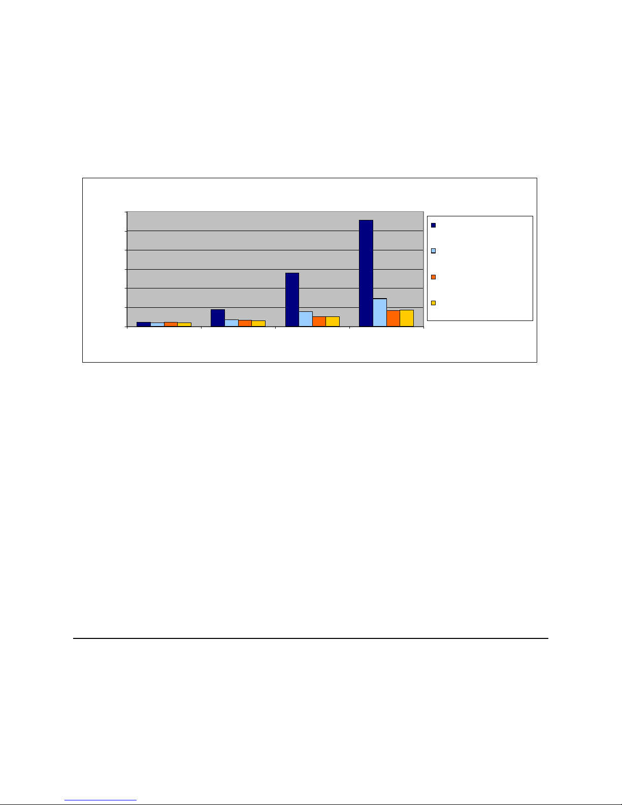
the statement is complete. The implementation to invoke the locking causes a physical DASD write to the journal for each record, which causes journal waits. Journal caching on allows the journal writes to accumulate in memory and have one DASD write per multiple journal entries, greatly reducing the journal wait time. So select from insert statements with FINAL TABLE run much faster with journal caching on. Figure 4.2 shows that select from insert with FINAL TABLE and journal caching on ran faster than the insert followed by select for all but the 1000 row insert size.

6.00

5.00

Select from Insert: Final Table

4.00

3.00

2.00

Clo ck Time Rat io

1.00

0.00

Select from I nsert / Insert t hen Select

1 10 100 1000

Records Inserted/Selected

Select from Insert: Final Table Journal caching on

Select from Ins ert: New Table

Select from Ins ert: New Table Journal caching on

Figure 4.2 Select from Insert versus Insert followed by Select clock time ratios

In addition to updates for new functionality, in V6R1 substantial performance improvements were made to some SQL code paths. Improvements were made to the optimizer to make query execution cost estimates more accurate. This means that the optimizer is producing more efficient access plans for some queries, which may reduce their run time. The time required to full open and optimize queries was also largely reduced for many queries in V6R1. On average, for a group of greatly varying queries, the total open time including optimization has been reduced 45%. For a given set of very simple queries which go through a full open, but whose access plan already exists in the plan cache, the full open time was reduced by up to 30%.

In addition to the optimization and full open performance improvements, for V6R1 there was a comprehensive effort to reduce the basic path of a simple query which is running in re-use mode (pseudo open), and in particular is using JDBC to access the database. The results of this are potentially large reductions in the CPU time used in processing queries, particularly very simple queries. For a stock trade workload running through JDBC, throughput improvements of up to 78% have been measured. For more information please see Chapter 6. Web Server and WebSphere Performance.

4.2 DB2 i5/OS V5R4 Highlights

In i5/OS V5R4 there were several performance enhancements to DB2 for i5/OS. With support in SQE for Like/Substring, LOBs and the use of temporary indexes, many more queries now go down the SQE path. Thus there is the potential for better performance due to the robust SQE optimizer choosing a better plan along with the more efficient query engine processing. Also supported is use of Recursive Common

IBM i 6.1 Performance Capabilities Reference - January/April/October 2008

Table Expressions (RCTE) which allow for more elegant and better performing implementations of recursive processing. In addition, enhancements have been made in i5/OS V5R4 to the support for materialize query tables (MQTs) and partitioned table processing, which were both new in i5/OS V5R3.

i5/OS V5R4 SQE Query Coverage

The query dispatcher controls whether an SQL query will be routed to SQE or to CQE. SQL queries with the following attributes, which were routed to CQE in previous releases, may now be routed to SQE in i5/OS V5R4:

y LOB columnsy Sensitive cursor y ALWCPYDTA(*NO)y Like/Substring predicates

SQL queries which continue to be routed to CQE in i5/OS V5R4 have the following attributes:

y DB2 Multisystemy References to DDS logical files y Tables with select/omit logicals over themy NLSS/CCSID translation between columns

y User-defined table unctions

In general, queries with Like and Substring predicates which are newly routed to SQE see substantial performance improvements in i5/OS V5R4. For a group of widely varying queries and data, including a wide range of Like and Substring predicates and various file sizes, a large percentage of the queries saw up to a 10X reduction in query run time. Queries with references to LOB columns, which were newly routed to SQE,, in general, also experience substantial performance improvements in i5/OS V5R4. For a set of queries which have references to LOB columns, in which the queries and data vary greatly a large percentage ran up to a 5X faster. .

A new addition to SQE is the creation and use of temporary indexes. These indexes will be created because they are required for implementing certain types of query requests or because they allow for better performance. The implementation of queries which require live data may require temporary indexes, for example, queries that run with a sensitive cursor or with ALWCPYDTA(*NO). In the case of using a temporary index for better performance, the SQE optimizer costs the creation and use of temporary indexes during plan optimization. An access plan will choose a temporary index if the amortized cost of building the index, provided one does not exist, reduces the query run time of the access plan enough that this plan wins over other plan options. The temporary indexes that the optimizer considers building are the same indexes in the ‘index advised’ list for a given query. Features unique to SQE temporary indexes, compared to CQE temporary indexes, are the longer lifetimes and higher degree of sharing of these indexes. SQE temporary indexes may be reused by the same query or other queries in the same job or in other jobs. The SQE temporary indexes will persist and will be maintained until the last query which references the temporary index is hard closed and the plan is removed from the plan cache. In many cases, this means the temporary indexes will persist until the last job which was using the index is ended. The high degree of sharing and longer lifetime allow for more reuse of the indexes without repeated create index cost.

New function for implementing applications that work with recursive data has been added to i5/OS V5R4. Recursive Common Table Expressions (RCTE) and Recursive Views may now be used in these types of applications, versus using SQL Stored Procedures and temporary results tables. For more information on using RCTEs and Recursive Views see the DB2 for System i Database Performance and Query Optimization manual.

IBM i 6.1 Performance Capabilities Reference - January/April/October 2008

Enhancements to extend the use of materialized query tables (MQTs) were added in i5/OS V5R4. New supported function in MQT queries by the MQT matching algorithm are unions and partitioned tables, along with limited support for scalar subselects, UDFs and user defined table functions, RCTE, and some scalar functions. Also new to i5/OS V5R4, the MQT matching algorithm now tries to match constants in the MQT with parameter markers or host variable values in the query. For more information on using MQTs see the DB2 for System i Database Performance and Query Optimization manual and the white paper, The creation and use of materialized query tables within IBM DB2 FOR i5/OS, available at

http://www-304.ibm.com/jct09002c/partnerworld/wps/servlet/ContentHandler/SROY-6UZ5E6

The performance of queries which reference partitioned tables has been enhanced in i5/OS V5R4. The overhead when optimizing queries which reference a partitioned table has been reduced. Additionally, general improvements in plan quality have yielded run time improvements as well.

4.3 i5/OS V5R3 Highlights

In i5/OS V5R3, the SQL Query Engine (SQE) roll-out in DB2 for i5/OS took the next step. The new SQL Query Optimizer, SQL Query Engine and SQL Database Statistics were introduced in V5R2 with a limited set of queries being routed to SQE. In i5/OS V5R3 many more SQL queries are implemented in SQE. In addition, many performance enhancements were made to SQE in i5/OS V5R3 to decrease query runtime and to use System i resources more efficiently. Additional significant new features in this release are: table partitioning, the lookahead predicate generation (LPG) optimization technique for enhanced star-join support and a technology preview of materialized query tables. Also an April 2005 addition to the DB2 FOR i5/OS V5R3 support was query optimizer support for recognizing and using materialized query tables (MQTs) (also referred to as automatic summary tables or materialized views) for limited query functions. Two other improvements worth mentioning are faster delete support and SQE constraint awareness. This section contains a summary of the V5R3 information in the System i Performance Capabilities Reference i5/OS Version 5 Release 3 available at

http://publib.boulder.ibm.com/infocenter/iseries/v5r3/topic/rzahx/sc410607.pdf

i5/OS V5R3 SQE Query Coverage

The query dispatcher controls whether an SQL query will be routed to SQE or to CQE (Classic Query Engine). The staged implementation of SQE enabled a very limited set of queries to be routed to SQE in V5R2. In general, read only single table queries with a limited set of attributes would be routed to SQE. The details of the query attributes for routing to SQE versus CQE in V5R2 are documented in the V5R2 redbook Preparing for and Tuning the V5R2 SQL Query Engine. With the V5R2 enabling PTF applied, PTF SI07650 documented in Info APAR II13486, the dispatcher routes many more queries through SQE. More single table queries and a limited set of multi-table queries are able to take advantage of the SQE enhancements. Queries with OR and IN predicates may be routed to SQE with the enabling PTF as will SQL queries with the appropriate attributes on systems with SMP enabled.

In i5/OS V5R3 a much larger set of queries are implemented in SQE including those with the enabling PTF on V5R2 and many queries with the following types of attributes:

y Unionsy Subqueries y Updates y Views y Deletesy Common table expressions

y Derived tables

IBM i 6.1 Performance Capabilities Reference - January/April/October 2008

SQL queries which continue to be routed to CQE in i5/OS V5R3 have the following attributes:

y NLSS/CCSID translation between columns y Sensitive cursor y DB2 Multisystemy Like/Substring predicates y ALWCPYDTA(*NO)y LOB columns y Tables with select/omit logicals over themy References to DDS logical files

i5/OS V5R3 SQE Performance Enhancements

Many enhancements were made in i5/OS V5R3 to enable faster query runtime and use less system resource. Highlights of these enhancements include the following:

y New optimization techniques including Lookahead Predication Generation and Constraint Awareness y Sharing of temporary result sets across jobs y Reduction in size of temporary result sets y More efficient I/O for temporary result sets y Ability to do some aggregates with EVI symbol table access only y Reduction in memory used during optimization y Reduction in DB structure memory usage y More efficient statistics generation during optimization y Greater accuracy of statistics usage for optimization plan generation

The DB2 performance enhancements in i5/OS V5R3 substantially reduced the runtime of many queries. Performance improvements vary substantially due to many factors -- file size and layout, indexes and statistics available -- making generalization of performance expectations for a given query difficult. However, longer running queries which are newly routed to SQE in i5/OS V5R3, in general, have a greater likelihood of significant performance benefit.

For the short running queries, those that run less than 2 seconds, performance improvements are nominal. For subsecond queries there is little to no improvement for most queries. As the runtime increases, the reduction in runtime and CPU time become more substantial. In general, for short running queries there is less opportunity for improving performance. Also, the first execution of all the queries in these figures was measured so that a database open and full optimization were required. Database open and full optimization overhead may be higher with SQE, as it evaluates more information and examines more potential query implementation plans. As this overhead is much more expensive relative to actual query implementation for short running queries, performance benefits from SQE for the short running queries are minimized. However, in OLTP environments the plan caching and open data path (ODP) reuse design minimizes the number of opens and full optimizations needed. A very small percentage of queries in typical customer OLTP workloads go through full open and optimization.

The performance benefits are substantial for many of the medium to long running queries newly routed to SQE in i5/OS V5R3. Typically, the longer the runtime, the more potential for improvements. This is due to the optimizer constructing a more efficient access plan and the faster execution of the access plan with the SQE query engine. Many of the queries with runtimes greater than 2 seconds, especially those with runtimes greater than 10 seconds, reduced their runtime by a factor of 2 or more. Queries which run longer than 200 seconds were typically improved from 15% to over 100 times.

IBM i 6.1 Performance Capabilities Reference - January/April/October 2008

Partitioned Table Support

Table partitioning is a new feature introduced in i5/OS V5R3. The design is localized on an individual table basis rather than an entire library. The user specifies one or more fields which collectively act as a partitioning key. Next the records in the table are distributed into multiple disjoint sets based on the partitioning scheme used: either a system-supplied hashing function or a set of value ranges (such as dates by month or year) supplied by the user. The user can partition data using up to 256 partitions in i5/OS V5R3. The partitions are stored as multiple members associated with the same file object, which continues to represent the overall table as a single entity from an SQL data-access viewpoint.

The primary motivations for the initial release of this feature are twofold:

y Eliminate the limitation of at most 4 billion (2^32) rows in a single table y Enhance data administration tasks such as save/restore, import/export, and add/drop which can be

done more quickly on a partition basis (subset of a table)

In theory, table partitioning also offers opportunities for performance gains on queries that specify selection referencing a single or small number of partitions. In reality, however, the performance impact of partitioned tables in this initial release are limited on the positive side and may instead result in performance degradation when adopted too eagerly without carefully considering the ramifications of such a change. The resulting performance after partitioning a table depends critically on the mix of queries used to access the table and the number of partitions created. If fields used as partitioning keys are frequently included in selection criteria the resulting performance can be much better due to improved locality of reference for the desired records. When used incorrectly, table partitioning may degrade the performance of queries by an order of magnitude or more -- particularly when a large number of partitions (>32) are created.

Performance expectations of table partitioning on i5/OS V5R3 should not

be equated at this time with partitioning concepts on other database platforms such as DB2 for Linux, Unix and Windows or offerings from other competitors. Nor should table partitioning on V5R3 be confused with the DB2 Multisystem for i5/OS offering. Carefully planned data storage schemes with active end-user disk arm management lead to the performance gains experienced with partitioned databases on those other platforms. Further gains are realized in other approaches through execution on clusters of physical nodes (in an approach similar to DB2 Multisystem for i5/OS). In addition, the entire schema is involved in the partitioning approach. On the other hand, the System i table partitioning design continues to utilize single level storage which already automatically spreads data to all disks in the relevant ASP. No new performance gains from I/O balancing are achieved when partitioning a table. Instead the gains tend to involve improved locality of reference for a subset of the data contained in a single partition or ease of administration when adding or deleting data on partition boundaries.

An in-depth discussion of table partitioning for i5/OS V5R3 is available in the white paper Table Partitioning Strategies for DB2 FOR i5/OS available at

http://www.ibm.com/servers/eserver/iseries/db2/awp.html

This publication covers additional details such as:

y Migration strategies for deployment y Requirements and Limitations y Sample Environments (OLTP, OLAP, Limits to Growth, etc.) & Recommended Settings y Indexing Strategies

IBM i 6.1 Performance Capabilities Reference - January/April/October 2008

y Statistical Strategies y SMP Considerations y Administration Examples (Adding a Partition, Dropping a Partition, etc.)

Materialized Query Table Support

The initial release of i5/OS V5R3 includes the Materialized Query Table (MQT) (also referred to as automatic summary tables or materialized views) support in UDB DB2 for i5/OS as essentially a technology preview. Pre-April 2005 i5/OS V5R3 provides the capability of creating materialized query tables, but no optimizer awareness of these MQTs. An April 2005 addition to DB2 for i5/OS V5R3 is query optimizer support for recognizing and using MQTs. This additional support for recognizing and using MQTs is limited to certain query functions. MQTs can provide performance enhancements in a manner similar to indexes. This is done by precomputing and storing results of a query in the materialized query table. The database engine can use these results instead of recomputing them for a user specified query. The query optimizer will look for any applicable MQTs and can choose to implement the query using a given MQT provided this is a faster implementation choice. For long running queries, the run time may be substantially improved with judicious use of MQTs. For more information on MQTs including how to enable this new support, for which queries support MQTs and how to create and use MQTs see the DB2 for System i Database Performance and Query Optimization manual. For the latest information on MQTs see http://www-1.ibm.com/servers/eserver/iseries/db2/mqt.html

Fast Delete Support

As developers have moved from native I/O to embedded SQL, they often wonder why a Clear Physical File Member (ClrPfm) command is faster than the SQL equivalent of DELETE FROM table. The reason is that the SQL DELETE statement deletes a single row at a time. In i5/OS V5R3, DB2 for System i has been enhanced with new techniques to speed up processing when every row in the table is deleted. If the DELETE statement is not run under commitment control, then DB2 for System i will actually use the ClrPfm operation underneath the covers. If the Delete is performed with commitment control, then DB2 FOR i5/OS can use a new method that’s faster than the old delete one row at a time approach. Note however that not all DELETEs will use the new faster support. For example, delete triggers are still processed the old way.

4.4 V5R2 Highlights - Introduction of the SQL Query Engine

In V5R2 major enhancements, entitled SQL Query Engine (SQE), were implemented in DB2 for i5/OS. SQE encompasses changes made in the following areas:

y SQL query optimizer y SQL query engine y Database statistics

A subset of the read-only SQL queries are able to take advantage of these enhancements in V5R2.

SQE Optimizer

The SQL query optimizer has been enhanced with new optimization capabilities implemented in object oriented technology. This object oriented framework implements new optimization techniques and allows for future extendibility of the optimizer. Among the new capabilities of the optimizer are enhanced query access plan costing. For queries which can take advantage of the SQE enhancements,

IBM i 6.1 Performance Capabilities Reference - January/April/October 2008

more information may be used in the query plan costing phase than was available to the optimizer previously. The optimizer may now use newly implemented database statistics to make more accurate decisions when choosing the query access plan. Also, the enhanced optimizer may more often select plans using hash tables and sorted partial result lists to hold partial query results during query processing, rather than selecting access plans which build temporary indexes. With less reliance on temporary indexes the SQE optimizer is able to select more efficient plans which save the overhead of building temporary indexes and more fully take advantage of single-level store. The optimizer changes were designed to create efficient query access plans for the enhanced database engine.

SQE Query Engine

The database engine is the part of the database implementation which executes the access plan produced by the query optimizer. It accesses the data, processes it, and returns the SQL query results. The new engine enhancements, the SQE database engine, employ state of the art object oriented implementation. The SQE database engine was developed in tandem with the SQE optimization enhancements to allow for an efficient design which is readily extendable. Efficient new algorithms for the data access methods are used in query processing by the SQE engine.

The basic data access algorithms in SQE are designed to take full advantage of the System i single-level store to give the fastest query response time. The algorithms reduce I/O wait time by making use of available main memory and aggressively reading data from disk into memory. The goal of the data read-ahead algorithms is that the data is in memory when it is needed. This is done through the use of asynchronous I/Os. SQL queries which access large amounts of data may see a considerable improvement in the query runtime. This may also result in higher peak disk utilization.

The effects of the SQE enhancements on SQL query performance will vary greatly depending on many factors. Among these factors are hardware configuration (processor, memory size, DASD configuration...), system value settings, file layout, indexes available, query options file QAQQINI settings, and the SQL queries being run.

SQE Database Statistics

The third area of SQE enhancements is the collection and use of new database statistics. Efficient processing of database queries depends primarily on a query optimizer that is able to make judicious choices of access plans. The ability of an optimizer to make a good decision is critically influenced by the availability of database statistics on tables referenced in queries. In the past such statistics were automatically gathered during optimization time for columns of tables over which indexes exist. With SQE statistics on columns without indexes can now be gathered and will be used during optimization. Column statistics comprise histograms, frequent values list, and column cardinality.

With System i servers, the database statistics collection process is handled automatically, while on many platforms statistics collection is a manual process that is the responsibility of the database administrator

. It

is rarely necessary for the statistics to be manually updated, even though it is possible to manage statistics manually. The Statistics Manager determines on what columns statistics are needed, when the statistics collection should be run and when the statistics need to be refreshed. Statistics are automatically collected as low priority work in the background, so as to minimize the impact to other work on the system. The manual collection of statistics is run with the normal user job priority.

The system automatically determines what columns to collect statistics on based on what queries have run on the system. Therefore for queries which have slower than expected performance results, a check

IBM i 6.1 Performance Capabilities Reference - January/April/October 2008

should be made to determine if the needed statistics are available. Also in environments where long running queries are run only one time, it may be beneficial to ensure that statistics are available prior to running the queries.

Some properties of database column statistics are as follows:

y Column statistics occupy little storage, on average 8-12k per column. y Column Statistics are gathered through one full scan of the database file for any given number of

columns in the database file.

y Column statistics are maintained periodically through means of statistics refreshing mechanisms

that require a full scan of the database file.

y Column statistics are packed in one concise data structure that requires few I/Os to page it into

main memory during query optimization.

As stated above, statistics may have a direct effect on the quality of the access plan chosen by the query optimizer and thereby influence the end user query performance. Shown below is an illustrative example that underscores the effect of statistics on access plan selection process.

Statistic Usage Example:

Select * from T1, T2 where T1.A=T2.A and T1.B = ’VALUE1’ and T2.C = ‘VALUE2’ Database characteristics: indexes on T1.A and T2.A exist, NO column statistics, T1 has 100 million rows,

T2 has 10 million rows. T1 is 1 GB and T2 0.1 GB Since statistics are not available, the optimizer has to consider default estimates for selectivity of T1.B =

’VALUE1’ ==> 10% T2.C = ‘VALUE2’ ==> 10% The actual estimates are T1.B = ’VALUE1’ ===>10% and T2.C = ‘VALUE2’ ===>0.00001% Based on selectivity estimates the optimizer will select the following access plan Scan(T1) - Probe (T2.A index) - > Probe (T2 Table) --the real cost for the above access plan would be approximately 8192 I/Os + 3600 I/Os ~ 11792 I/Os If column statistics existed on T2.C the selectivity estimate for T2.C = ‘VALUE2’ would be 10 rows or

0.00001% And the query optimizer would select the following plan instead Scan(T2) - Probe (T1.A index) - > Probe (T1 Table) Accordingly the real cost could be calculated as follows: 819 I/Os + 10 I/Os ~ 830 I/Os. The result of having statistics on T2.C led to an access plan that is

faster by order of magnitude from a case where no statistics exist.

For more information on database statistics collection see the DB2 for i5/OS Database Performance and Query Optimization manual.

IBM i 6.1 Performance Capabilities Reference - January/April/October 2008

SQE for V5R2 Summary

Enhancements to DB2 for i5/OS, called SQE, were made in V5R2. The SQE enhancements are object oriented implementations of the SQE optimizer, the SQE query engine and the SQE database statistics. In V5R2 a subset of the read-only SQL queries will be optimized and run with the SQE enhancements. The effect of SQE on performance will vary by workload and configuration. For the most recent information on SQE please see the SQE web page on the DB2 for i5/OS web site located at

www.iseries.ibm.com/db2/sqe.html.

More information on SQE for V5R2 is also available in the V5R2

redbook Preparing for and Tuning the V5R2 SQL Query Engine.

4.5 Indexing

Index usage can dramatically improve the performance of DB2 SQL queries. For detailed information on using indexes see the white paper Indexing Strategies for DB2 for i5/OS at

http://www-1.ibm.com/servers/enable/site/education/abstracts/indxng_abs.html

information about indexes in DB2 for i5/OS, the data structures underlying them, how the system uses them and index strategies. Also discussed are the additional indexing considerations related to maintenance, tools and methods.

Encoded Vector Indices (EVIs)

DB2 for i5/OS supports the Encoded Vector Index (EVI) which can be created through SQL. EVIs cannot be used to order records, but in many cases, they can improve query performance. An EVI has several advantages over a traditional binary radix tree index.

. The paper provides basic

y The query optimizer can scan EVIs and automatically build dynamic (on-the-fly) bitmaps much more

quickly than from traditional indexes.

y EVIs can be built much faster and are much smaller than traditional indexes. Smaller indexes require

less DASD space and also less main storage when the query is run.

y EVIs automatically maintain exact statistics about the distribution of key values, whereas traditional

indexes only maintain estimated statistics. These EVI statistics are not only more accurate, but also can be accessed more quickly by the query optimizer.

EVIs are used by the i5/OS query optimizer with dynamic bitmaps and are particularly useful for advanced query processing. EVIs will have the biggest impact on the complex query workloads found in business intelligence solutions and ad-hoc query environments. Such queries often involve selecting a limited number of rows based on the key value being among a set of specific values (e.g. a set of state names).

When an EVI is created and maintained, a symbol table records each distinct key value and also a corresponding unique binary value (the binary value will be 1, 2, or 4 bytes long, depending on the number of distinct key values) that is used in the main part of the EVI, the vector (array). The subscript of each vector (array) element represents the relative record number of a database table row. The vector has an entry for each row. The entry in each element of the vector contains the unique binary value corresponding to the key value found in the database table row.

IBM i 6.1 Performance Capabilities Reference - January/April/October 2008

4.6 DB2 Symmetric Multiprocessing feature

Introduction

The DB2 SMP feature provides application transparent support for parallel query operations on a single tightly-coupled multiprocessor System i (shared memory and disk). In addition, the symmetric multiprocessing (SMP) feature provides additional query optimization algorithms for retrieving data. The database manager can automatically activate parallel query processing in order to engage one or more system processors to work simultaneously on a single query. The response time can be dramatically improved when a processor bound query is executed in parallel on multiple processors. For more information on access methods which use the SMP feature and how to enable SMP see the DB2 for i5/OS Database Performance and Query Optimization manual in the System i information center.

Decision Support Queries

The SMP feature is most useful when running decision support (DSS) queries. DSS queries which generally give answers to critical business questions tend to have the following characteristics:

y examine large volumes of data y are far more complex than most OLTP transactions y are highly CPU intensive y includes multiple order joins, summarizations and groupings

DSS queries tend to be long running and can utilize much of the system resources such as processor capacity (CPU) and disk. For example, it is not unusual for DSS queries to have a response time longer than 20 seconds. In fact, complex DSS queries may run an hour or longer. The CPU required to run a DSS query can easily be 100 times greater than the CPU required for a typical OLTP transaction. Thus, it is very important to choose the right System i for your DSS query and data warehousing needs.

SMP Performance Summary

The SMP feature provides performance improvement for query response times. The overall response time for a set of DSS queries run serially at a single work station may improve more than 25 percent when SMP support is enabled. The amount of improvement will depend in part on the number of processors participating in each query execution and the optimization algorithms used to implement the query. Some individual queries can see significantly larger gains.

An online course, DB2 Symmetric Multiprocessing for System i: Database Parallelism within i5/OS, including a pdf form of the course materials is available at

http://www-03.ibm.com/servers/enable/site/education/ibp/4aea/index.html

4.7 DB2 for i5/OS Memory Sharing Considerations

DB2 for i5/OS has internal algorithms to automatically manage and share memory among jobs. This eliminates the complexity of setting and tuning many parameters which are essential to getting good performance on other database products. The memory sharing algorithms within SQE and i5/OS will limit the amount of memory available to execute an SQL query to a ‘job share’. The optimizer will choose an access plan which is optimal for the job’s share of the memory pool and the query engine will

IBM i 6.1 Performance Capabilities Reference - January/April/October 2008

limit the amount of data it brings into and keeps in memory to a job’s share of memory. The amount of memory available to each job is inversely proportional to the number of active jobs in a memory pool.

The memory-sharing algorithms discussed above provide balanced performance for all the jobs running in a memory pool. Running short transactional queries in the same memory pool as long running, data intensive queries is acceptable. However, if it is desirable to get maximum performance for long-running, data-intensive queries it may be beneficial to run these types of queries in a memory pool dedicated to this type of workload. Executing long-running, data-intensive queries in the same memory pool with a large volume of short transactional queries will limit the amount of memory available for execution of the long-running query. The plan choice and engine execution of the long-running query will be tuned to run in the amount of memory comparable to that available to the jobs running the short transactional queries. In many cases, data-intensive, long-running queries will get improved performance with larger amounts of memory. With more memory available the optimizer is able to consider access plans which may use more memory, but will minimize runtime. The query engine will also be able to take advantage of additional memory by keeping more data in memory potentially eliminating a large number of DASD I/Os. Also, for a job executing long-running performance critical queries in a separate pool, it may be beneficial to set QQRYDEGREE=*MAX. This will allow all memory in the pool to be used by the job to process a query. Thus running the longer-running, data intensive queries in a separate pool may dramatically reduce query runtime.

4.8 Journaling and Commitment Control

Journaling

The primary purpose of journal management is to provide a method to recover database files. Additional uses related to performance include the use of journaling to decrease the time required to back up database files and the use of access path journaling for a potentially large reduction in the length of abnormal IPLs. For more information on the uses and management of journals, refer to the Sytem i Backup and Recovery Guide. For more detailed information on the performance impact of journaling see

the redbook Striving for Optimal Journal Performance on DB2 Universal Database for System i.

The addition of journaling to an application will impact performance in terms of both CPU and I/O as the application changes to the journaled file(s) are entered into the journal. Also, the job that is making the changes to the file must wait for the journal I/O to be written to disk, so response time will in many cases be affected as well.

Journaling impacts the performance of each job differently, depending largely on the amount of database writes being done. Applications doing a large number of writes to a journaled file will most likely show a significant degradation both in CPU and response time while an application doing only a limited number of writes to the file may show only a small impact.

Remote Journal Function

The remote journal function allows replication of journal entries from a local (source) System i to a remote (target) System i by establishing journals and journal receivers on the target system that are associated with specific journals and journal receivers on the source system. Some of the benefits of using remote journal include:

IBM i 6.1 Performance Capabilities Reference - January/April/October 2008

y Allows customers to replace current programming methods of capturing and transmitting journal

entries between systems with more efficient system programming methods. This can result in lower CPU consumption and increased throughput on the source system.

y Can significantly reduce the amount of time and effort required by customers to reconcile their source

and target databases after a system failure. If the synchronous delivery mode of remote journal is used (where journal entries are guaranteed to be deposited on the target system prior to control being returned to the user application), then there will be no journal entries lost. If asynchronous delivery mode is used, there may be some journal entries lost, but the number of entries lost will most likely be fewer than if customer programming methods were used due to the reduced system overhead of remote journal.

y Journal receiver save operations can be offloaded from the source system to the target system, thus

further reducing resource and consumption on the source system.

Hot backup, data replication and high availability applications are good examples of applications which can benefit from using remote journal. Customers who use related or similar software solutions from other vendors should contact those vendors for more information.

System-Managed Access Path Protection (SMAPP)

System-Managed Access Path Protection (SMAPP) offers system monitoring of potential access path rebuild time and automatically starts and stops journaling of system selected access paths. In the unlikely event of an abnormal IPL, this allows for faster access path recovery time.

SMAPP does implicit access path journaling which provides for limited partial/localized recovery of the journaled access paths. This provides for much faster IPL recovery steps. An estimation of how long access path recovery will take is provided by SMAPP, and SMAPP provides a setting for the acceptable length of recovery. SMAPP is shipped enabled with a default recovery time. For most customers, the default value will minimize the performance impact, while at the same time provide a reasonable and predictable recovery time and protection for critical access paths. But the overhead of SMAPP will vary from system to system and application to application. As the target access path recovery time is lowered, the performance impact from SMAPP will increase as the SMAPP background tasks have to work harder to meet this target. There is a balance of recovery time requirements vs. the system resources required by SMAPP.

Although SMAPP may start journaling access paths, it is recommended that the most important/large/critical/performance sensitive access paths be journaled explicitly with STRJRNAP. This eliminates the extra overhead of SMAPP evaluating these access paths and implicitly starting journaling for the same access path day after day. A list of the currently protected access paths may be seen as an option from the DSPRCYAP screen. Indexes which consistently show up at the top of this list may be good candidates for explicit journaling via the STRJRNAP command. As identifying important access paths can be a difficult task, SMAPP provides a good safety net to protect those not explicitly journaled.

In addition to the setting to specify a target recovery time, SMAPP also has the following special settings which may be selected with the EDTRCYAP and CHGRCYAP commands:

y *MIN - all exposed indexes will be protected y *NONE - no indexes will be protected; SMAPP statistics will be maintained y *OFF - no indexes will be protected; No SMAPP statistics will be maintained (Restricted Mode)

It is highly recommended that SMAPP protection NOT be turned off.

IBM i 6.1 Performance Capabilities Reference - January/April/October 2008

There are 3 sets of tasks which do the SMAPP work. These tasks work in the background at low priority to minimize the impact of SMAPP on system performance. The tasks are as follows: y JO_EVALUATE-TASK - Evaluates indexes, estimates rebuild time for an index, and may start or

stop implicit journaling of an index.

y JO-TUNING-TASK - Periodically wakes up to consider where the user recovery threshold is set and

manages which indexes should be implicitly journaled.

y JORECRA-DEF-XXX and JORECRA-USR-XXX tasks are the worker tasks which sweep aged

journal pages from main memory to minimize the amount of recovery needed during IPL.

Here are guidelines for lowering the amount of work for each of these tasks:

y If the JO-TUNING-TASK seems busy, you may want to increase SMAPP recovery target time. y If the JO-EVALUATE task seems busy, explicitly journaling the largest access paths may help or

looks for jobs that are opening/closing files repeatedly.

y If the JORECRA tasks seem busy, you may want to increase journal recovery ratio. y Also, if the target recovery time is not being met there may be SMAPP ineligible access paths. These

should be modified so as to become SMAPP eligible.

To monitor the performance impacts of SMAPP there are Performance Explorer trace points and a substantial set of Collection Services counters which provide information on the SMAPP work.

SMAPP makes a decision of where to place the implicit access path journal entries. If the underlying physical file is not journaled, SMAPP will place the entries in a default (hidden) system journal. If the underlying physical file is journaled, SMAPP will place the implicit journal entries in the same place. SMAPP automatically manages the system journal. For the user journal receivers used by SMAPP, RCVSIZOPT(*RMVINTENT), as specified on the CHGJRN command, is a recommended option. The disk space used by SMAPP may be displayed with the EDTRCYAP and DSPRCYAP commands. It rarely exceeds 1% of the ASP size.

For more information on SMAPP see the Systems management -> Journal management -> System-managed access path protection section in the System i information center.

Commitment Control

Commitment control is an extension to the journal function that allows users to ensure that all changes to a transaction are either all complete or, if not complete, can be easily backed out. The use of commitment control adds two more journal entries, one at the beginning of the committed transaction and one at the end, resulting in additional CPU and I/O overhead. In addition, the time that record level locks are held increases with the use of commitment control. Because of this additional overhead and possible additional record lock contention, adding commitment control will in many cases result in a noticeable degradation in performance for an application that is currently doing journaling.

4.9 DB2 Multisystem for i5/OS

DB2 Multisystem for i5/OS offers customers the ability to distribute large databases across multiple System i servers in order to gain nearly unlimited scalability and improved performance for many large query operations. Multiple System i servers are coupled together in a shared-nothing cluster where each system uses its own main memory and disk storage. Once a database is properly partitioned among the

IBM i 6.1 Performance Capabilities Reference - January/April/October 2008

multiple nodes in the cluster, access to the database files is seamless and transparent to the applications and users that reference the database. To the users, the partitioned files still behave as though they were local to their system.

The most important aspect of obtaining optimal performance with DB2 Multisystem is to plan ahead for what data should be partitioned and how it should be partitioned. The main idea behind this planning is to ensure that the systems in the cluster run in parallel with each other as much as possible when processing distributed queries while keeping the amount of communications data traffic to a minimum. Following is a list of items to consider when planning for the use of distributed data via DB2 Multisystem.

y Avoid large amounts of data movement between systems. A distributed query often achieves optimal

performance when it is able to divide the query among several nodes, with each node running its portion of the query on data that is local to that system and with a minimum number of accesses to remote data on other systems. Also, if a file that is heavily used for transaction processing is to be distributed, it should be done such that most of the database accesses are local since remote accesses may add significantly to response times.

y Choosing which files to partition is important. The largest improvements will be for queries on large

files. Files that are primarily used for transaction processing and not much query processing are generally not good candidates for partitioning. Also, partitioning files with only a small number of records will generally not result in much improvement and may actually degrade performance due to the added communications overhead.

y Choose a partitioning key that has many different values. This will help ensure a more even

distribution of the data across the multiple nodes. In addition, performance will be best if the partitioning key is a single field that is a simple data type.

y It is best to choose a partition key that consists of a field or fields whose values are not updated.

Updates on partition keys are only allowed if the change to the field(s) in the key will not cause that record to be partitioned to a different node.

y If joins are often performed on multiple files using a single field, use that field as the partitioning key

for those files. Also, the fields used for join processing should be of the same data type.

y It will be helpful to partition the database files based on how quickly each node can process its

portion of the data when running distributed queries. For example, it may be better to place a larger amount of data on a large multiprocessor system than on a smaller single processor system. In addition, current normal utilization levels of other resources such as main memory, DASD and IOPs should be considered on each system in order to ensure that no one individual system becomes a bottleneck for distributed query performance.

y For the best query performance involving distributed files, avoid the use of commitment control when

possible. DB2 Multisystem uses two-phase commit, which can add a significant amount of overhead when running distributed queries.

For more information on DB2 Multisystem refer to the DB2 Multisystem manual.

IBM i 6.1 Performance Capabilities Reference - January/April/October 2008

4.10 Referential Integrity

In a database user environment, there are frequent cases where the data in one file is dependent upon the data in another file. Without support from the database management system, each application program that updates, deletes or adds new records to the files must contain code that enforces the data dependency rules between the files. Referential Integrity (RI) is the mechanism supported by DB2 that offers its users the ability to enforce these rules without specifically coding them in their application(s). The data dependency rules are implemented as referential constraints via either CL commands or SQL statements that are available for adding, removing and changing these constraints.

For those customers that have implemented application checking to maintain integrity of data among files, there may be a noticeable performance gain when they change the application to use the referential integrity support. The amount of improvement depends on the extent of checking in the existing application. Also, the performance gain when using RI may be greater if the application currently uses SQL statements instead of HLL native database support to enforce data dependency rules.

When implementing RI constraints, customers need to consider which data dependencies are the most commonly enforced in their applications. The customer may then want to consider changing one or more of these dependencies to determine the level of performance improvement prior to a full scale implementation of all data dependencies via RI constraints.

For more information on Referential Integrity see the chapter Ensuring Data Integrity with Referential

Constraints in DB2 Universal Database for System i Database Programming Advanced Functions and Administration on DB2 Universal Database for System i.

manual and the redbook

4.11 Triggers

Trigger support for DB2 allows a user to define triggers (user written programs) to be called when records in a file are changed. Triggers can be used to enforce consistent implementation of business rules for database files without having to add the rule checking in all applications that are accessing the files. By doing this, when the business rules change, the user only has to change the trigger program.

There are three different types of events in the context of trigger programs: insert, update and delete. Separate triggers can be defined for each type of event. Triggers can also be defined to be called before or after the event occurs.

Generally, the impact to performance from applying triggers on the same system for files opened without commitment control is relatively low. However, when the file(s) are under commitment control, applying triggers can result in a significant impact to performance.

Triggers are particularly useful in a client server environment. By defining triggers on selected files on the server, the client application can cause synchronized, systematic update actions to related files on the server with a single request. Doing this can significantly reduce communications traffic and thus provide noticeably better performance both in terms of response time and CPU. This is true whether or not the file is under commitment control.

IBM i 6.1 Performance Capabilities Reference - January/April/October 2008

The following are performance tips to consider when using triggers support:

y Triggers are activated by an external call. The user needs to weigh the benefit of the trigger against

the cost of the external call.

y If a trigger is going to be used, leave as much validation to the trigger program as possible.

y Avoid opening files in a trigger program under commitment control if the trigger program does not

cause changes to commitable resources.

y Since trigger programs are called repeatedly, minimize the cost of program initialization and

unneeded repeated actions. For example, the trigger program should not have to open and close a file every time it is called. If possible, design the trigger program so that the files are opened during the first call and stay open throughout. To accomplish this, avoid SETON LR in RPG, STOP RUN in COBOL and exit() in C.

y If the trigger program opens a file multiple times (perhaps in a program which it calls), make use of

shared opens whenever possible.

y If the trigger program is written for the Integrated Language Environment (ILE), make sure it uses the

caller's activation group. Having to start a new activation group every time the time the trigger program is called is very costly.

y If the trigger program uses SQL statements, it should be optimized such that SQL makes use of

reusable ODPs.

In conclusion, the use of triggers can help enforce business rules for user applications and can possibly help improve overall system performance, particularly in the case of applying changes to remote systems. However, some care needs to be used in designing triggers for good performance, particularly in the cases where commitment control is involved. For more information see the redbook Stored Procedures,

Triggers and User Defined Functions on DB2 Universal Database for System i.

4.12 Variable Length Fields

Variable length field support allows a user to define any number of fields in a file as variable length, thus potentially reducing the number of bytes that need to be stored for a particular field.

Description

Variable length field support on i5/OS has been implemented with a spill area, thus creating two possible situations: the non-spill case and the spill case. With this implementation, when the data overflows, all of the data is stored in the spill portion. An example would be a variable length field that is defined as having a maximum length of 50 bytes and an allocated length of 20 bytes. In other words, it is expected that the majority of entries in this field will be 20 bytes or less and occasionally there will be a longer entry up to 50 bytes in length. When inserting an entry that has a length of 20 bytes or less that entry will be inserted into the allocated part of the field. This is an example of a non-spill case. However, if an entry is inserted that is, for example, 35 bytes long, all 35 bytes will go into the spill area.

IBM i 6.1 Performance Capabilities Reference - January/April/October 2008

To create the variable length field just described, use the following DB2 statement:

CREATE TABLE library/table-name (field VARCHAR(50) ALLOCATE(20) NOT NULL)

In this particular example the field was created with the NOT NULL option. The other two options are NULL and NOT NULL WITH DEFAULT. Refer to the NULLS section in the SQL Reference to determine which NULLS option would be best for your use. Also, for additional information on variable length field support, refer to either the SQL Reference or the SQL Programming Concepts.

Performance Expectations

y Variable length field support, when used correctly, can provide performance improvements in many

environments. The savings in I/O when processing a variable length field can be significant. The biggest performance gains that will be obtained from using variable length fields are for description or comment types of fields that are converted to variable length. However, because there is additional overhead associated with accessing the spill area, it is generally not a good idea to convert a field to variable length if the majority (70-100%) of the records would have data in this area. To avoid this problem, design the variable length field(s) with the proper allocation length so that the amount of data in the spill area stays below the 60% range. This will also prevent a potential waste of space with the variable length implementation.

y Another potential savings from the use of variable length fields is in DASD space. This is particularly

true in implementations where there is a large difference between the ALLOCATE and the VARCHAR attributes AND the amount of spill data is below 60%. Also, by minimizing the size of the file, the performance of operations such as CPYF (Copy File) will also be improved.

y When using a variable length field as a join field, the impact to performance for the join will depend

on the number of records returned and the amount of data that spills. For a join field that contains a low percentage of spill data and which already has an index built over it that can be used in the join, a user would most likely find the performance acceptable. However, if an index must be built and/or the field contains a large amount of overflow, a performance problem will likely occur when the join is processed.

y Because of the extra processing that is required for variable length fields, it is not a good idea to

convert every field in a file to variable length. This is particularly true for fields that are part of an index key. Accessing records via a variable length key field is noticeably slower than via a fixed length key field. Also, index builds over variable length fields will be noticeably slower than over fixed length fields.

y When accessing a file that contains variable length fields through a high-level language such as

COBOL, the variable that the field is read into must be defined as variable or of a varying length. If this is not done, the data that is read in to the fixed length variable will be treated as fixed length. If the variable is defined as PIC X(40) and only 25 bytes of data is read in, the remaining 15 bytes will be space filled. The value in that variable will now contain 40 bytes. The following COBOL example shows how to declare the receiving variable as a variable length variable:

IBM i 6.1 Performance Capabilities Reference - January/April/October 2008

01 DESCR.

49 DESCR-LEN PIC S9(4) COMP-4. 49 DESCRIPTION PIC X(40).

EXEC SQL FETCH C1 INTO DESCR END-EXEC.

For more detail about the vary-length character string, refer to the SQL Programmer's Guide.

The above point is also true when using a high-level language to insert values into a variable length field. The variable that contains the value to be inserted must be declared as variable or varying. A PL/I example follows:

DCL FLD1 CHAR(40) VARYING;

FLD1 = XYZ Company;

EXEC SQL INSERT INTO library/file VALUES ("001453", FLD1, ...);

Having defined FLD1 as VARYING will, for this example, insert a data string of 11 bytes into the field corresponding with FLD1 in this file. If variable FLD1 had not been defined as VARYING, a data string of 40 bytes would be inserted into the corresponding field. For additional information on the VARYING attribute, refer to the PL/I User's Guide and Reference.

y In summary, the proper implementation and use of DB2 variable length field support can help provide

overall improvements in both function and performance for certain types of database files. However, the amount of improvement can be greatly impacted if the new support is not used correctly, so users need to take care when implementing this function.

4.13 Reuse Deleted Record Space

Description of Function

This section discusses the support for reuse of deleted record space. This database support provides the customer a way of placing newly-added records into previously deleted record spaces in physical files. This function should reduce the requirement for periodic physical file reorganizations to reclaim deleted record space. File reorganization can be a very time consuming process depending on the size of the file and the number of indexes over it, along with the reorganize options selected. To activate the reuse function, set the Reuse deleted records (REUSEDLT) parameter to *YES on the CRTPF (Create Physical File) The default value when creating a file with CRTPF is *NO (do not reuse). The default for SQL Create Table is *YES.

Comparison to Normal Inserts

Inserts into deleted record spaces are handled differently than normal inserts and have different performance characteristics. For normal inserts into a physical file, the database support will find the end of the file and seize it once for exclusive use for the subsequent adds. Added records will be written in blocks at the end of the file. The size of the blocks written will be determined by the default block size or by the size specified using an Override Database File (OVRDBF) command. The SEQ(*YES number of records) parameter can be used to set the block size.

IBM i 6.1 Performance Capabilities Reference - January/April/October 2008

In contrast, when reuse is active, the database support will process the added record more like an update operation than an add operation. The database support will maintain a bit map to keep track of deleted records and to provide fast access to them. Before a record can be added, the database support must use the bit-map to find the next available deleted record space, read the page containing the deleted record entry into storage, and seize the deleted record to allow replacement with the added record. Lastly, the added records are blocked as much as permissible and then written to the file.

To summarize, additional CPU processing will be required when reuse is active to find the deleted records, perform record level seizes and maintain the bit-map of deleted records. Also, there may be some additional disk I/O required to read in the deleted records prior to updating them. However, this extra overhead is generally less than the overhead associated with a sequential update operation.

Performance Expectations

The impact to performance from implementing the reuse deleted records function will vary depending on the type of operation being done. Following is a summary of how this function will affect performance for various scenarios:

y When blocking was not specified, reuse was slightly faster or equivalent to the normal insert

application. This is due to the fact that reuse by default blocks up records for disk I/Os as much as possible.

y Increasing the number of indexes over a file will cause degradation for all insert operations,

regardless of whether reuse is used or not. However, with reuse activated, the degradation to insert operations from each additional index is generally higher than for normal inserts.

y The RGZPFM (Reorganize Physical File Member) command can run for a long period of time,

depending on the number of records in the file and the number of indexes over the file and the chosen command options. Even though activating the reuse function may cause some performance degradation, it may be justified when considering reorganization costs to reclaim deleted record space.

y The reuse function can always be deactivated if the customer encounters a critical time window where

no degradation is permissible. The cost of activating/de-activating reuse is relatively low in most cases.

y Because the reuse function can lead to smaller sized files, the performance of some applications may

actually improve, especially in cases where sequential non-keyed processing of a large portion of the file(s) is taking place.

4.14 Performance References for DB2

1. The home page for DB2 Universal Database for System i is found at

http://www-1.ibm.com/servers/eserver/iseries/db2/

This web site includes the recent announcement information, white paper and technical articles, and DB2 education information.

IBM i 6.1 Performance Capabilities Reference - January/April/October 2008

2. The System i information center section on DB2 for i5/OS under Database and file systems has

information on all aspects of DB2 for i5/OS including the section Monitor and Tune database under Administrative topics. This can be found at url:

http://www.ibm.com/eserver/iseries/infocenter

3. Information on creating efficient running queries and query performance monitoring and tuning is

found in the DB2 for i5/OS Database Performance and Query Optimization manual. This document contains detailed information on access methods, the query optimizer, and optimizing query performance including using database monitor to monitor queries, using QAQQINI file options and using indexes. To access this document look in the Printable PDF section in the System i information center.

4. The System i redbooks provide performance information on a variety of topics for DB2. The redbook

repository is located at http://publib-b.boulder.ibm.com/Redbooks.nsf/portals/systemi

IBM i 6.1 Performance Capabilities Reference - January/April/October 2008

Chapter 5. Communications Performance

There are many factors that affect System i performance in a communications environment. This chapter discusses some of the common factors and offers guidance on how to help achieve the best possible performance. Much of the information in this chapter was obtained as a result of analysis experience within the Rochester development laboratory. Many of the performance claims are based on supporting performance measurement and analysis with the NetPerf and Netop workloads. In some cases, the actual performance data is included here to reinforce the performance claims and to demonstrate capacity characteristics. The NetPerf and Netop workloads are described in section 5.2.

This chapter focuses on communication in non-secure and secure environments on Ethernet solutions using TCP/IP. Many applications require network communications to be secure. Communications and cryptography, in these cases, must be considered together. Secure Socket Layer (SSL), Transport Layer Security (TLS) and Virtual Private Networking (VPN) capacity characteristics will be discussed in section 5.5 of this chapter. For information about how the Cryptographic Coprocessor improves performance on SSL/TLS connections, see section 8.4 of Chapter 8, “Cryptography Performance.”

Communications Performance Highlights for IBM i Operation System 5.4:

y The support for the new Internet Protocol version 6 (IPv6) has been enhanced. The new IPv6

functions are consistent at the product level with their respective IPv4 counterparts.

y Support is added for the 10 Gigabit Ethernet optical fiber input/output adapters (IOAs) 573A and

576A. These IOAs do not require an input/output processor (IOP) to be installed in conjunction with the IOA. Instead the IOA can be plugged into a PCI bus slot and the IOA is controlled by the main processor. The 573A is a 10 Gigabit SR (short reach) adapter, which uses multimode fiber (MMF) and has a duplex LC connector. The 573A can transmit to lengths of 300 meters. The 576A is a 10 Gigabit LR (long reach) adapter, which uses single mode fiber (SMF) and has a duplex SC connector. The 576A can transmit to lengths of 10 kilometers. Both of these adapters support TCP/IP, 9000-byte jumbo frames, checksum offloading and the IEEE 802.3ae standard.

y The IBM 5706 2-Port 10/100/1000 Base-TX PCI-X IOA and IBM 5707 2-Port Gigabit Ethernet-SX

PCI-X IOA supports checksum offloading and 9000-byte jumbo frames (1 Gigabit only). These adapters do not require an IOP to be installed in conjunction with the IOA.

y The IBM 5701 10/100/1000 Base-TX PCI-X IOA does not require an IOP to be installed in

conjunction with the IOA.

y The IBM Cryptographic Access Provider product, 5722-AC3 (128-bit) is no longer required. This is

a new development for the 5.4 release of IBM i Operation System. All 5.4 systems are capable of the function that was previously provided in the 5722-AC3 product. This is relevant for SSL communications.

Communications Performance Highlights for IBM i Operation System 5.4.5:

y The IBM 5767 2-Port 10/100/1000 Based-TX PCI-E IOA and IBM 5768 2-Port Gigabit Ethernet-SX

PCI-E IOA supports checksum offloading and 9000-byte jumbo frames (1 Gigabit only). These adapters do not require an IOP to be installed in conjunction with the IOA.

IBM i 6.1 Performance Capabilities Reference - January/April/October 2008

y IBM’s Host Ethernet Adapter (HEA) integrated 2-Port 10/100/1000 Based-TX PCI-E IOA supports

checksum offloading, 9000-byte jumbo frames (1 Gigabit only) and LSO - Large Send Offload (IPv4 only). These adapters do not require an IOP to be installed in conjunction with the IOA. Additionally, each physical port has 16 logical ports that may be assigned to other partitions and allows each partition to utilize the same physical port simultaneously with the following limitation: one logical port, per physical port, per partition.

Communications Performance Highlights for IBM i Operation System 6.1:

y Additional enhancement in Internet Protocol version 6 (IPv6) in the following areas:

1. Advanced Sockets APIs

2. Path MTU Discovery

3. Correspondent Node Mobility Support

4. Support of Privacy extensions to stateless address auto-configuration

5. Virtual IP address,

6. Multicast Listener Discovery v2 support

7. Router preferences and more specific route advertisement support

8. Router load sharing.

y Additional enhancement in Internet Protocol version 4 (IPv4) in the following areas:

1. Remote access proxy fault tolerance

2. IGMP v3 support for IPv4 multicast.

y Large Send Offload support was implemented for Host Ethernet Adapter ports on Internet Protocol

version 4 (IPv4).

5.1 System i Ethernet Solutions

The need for communication between computer systems has grown over the last decades, and TCP/IP over Ethernet has grown with it. We currently have arrived where different factors influence the capabilities of the Ethernet. Some of these influences can come from the cabling and adapter type chosen. Limiting factors can be the capabilities of the hub or switch used, the frame size you are able to transmit and receive, and the type of connection used. The System i server is capable of transmitting and receiving data at speeds of 10 megabits per second (10 Mbps) to 10 gigabits per second (10 Gbps or 10 000 Mbps) using an Ethernet IOA. Functions such as full duplex also enhance the communication speeds and the overall performance of Ethernet.

Table 5.1 contains a list of Ethernet input/output adapters that are used to create the results in this chapter.

Table 5.1

Ethernet input/output adapters

5706 5707 5767 5768

1 2 1 1 2 1 2

DescriptionCCIN

Speed

(Mbps)

Jumbo

frames

supported

Console

supported

Duplex mode capabilityOperations

HalfFull

YesYesYesNo10 / 10010/100 Mbps Ethernet2849

NoYesNoYes1000IBM Gigabit Ethernet-SX PCI-X5700 YesYesNoYes10 / 100 / 1000IBM 10/100/1000 Base-TX PCI-X5701 YesYesYesYes10 / 100 / 1000IBM 2-Port 10/100/1000 Base-TX PCI-X

NoYesYesYes1000IBM 2-Port Gigabit Ethernet-SX PCI-X YesYesYesYes10 / 100 / 1000IBM 2-Port 10/100/1000 Base-TX PCI-e

NoYesYesYes1000IBM 2-Port Gigabit Ethernet-SX PCI-e

NoYesNoYes10000IBM 10 Gigabit Ethernet-SX PCI-X573A

IBM i 6.1 Performance Capabilities Reference - January/April/October 2008

181A

2 1

181C

1819

Virtual Ethernet

N/A N/A

Notes:

1. Unshielded Twisted Pair (UTP) card; uses copper wire cabling

2. Uses fiber optics

3. Custom Card Identification Number and System i Feature Code

4. Virtual Ethernet enables you to establish communication via TCP/IP between logical partitions and can be used without any additional hardware or software.

5. Depends on the hardware of the system.

6. These are theoretical hardware unidirectional speeds

7. Each port can handle 1000 Mbps

8. Blade communicates with the VIOS Partition via Virtual Ethernet

9. Host Ethernet Adapter for IBM Power 550, 9409-M50 running IBM i Operating System

y All adapters support Auto-negotiation

Blade

7 7,9

5 5

YesYesYesYes10 / 100 / 1000IBM 2-Port 10/100/1000 Base-TX PCI-e YesYesYesYes10000IBM 2-Port Gigabit Base-SX PCI-e181B YesYesYesYes10 / 100 / 1000IBM 4-Port 10/100/1000 Base-TX PCI-e YesYesYesYes10 / 100 / 1000IBM 4-Port 10/100/1000 Base-TX PCI-e

YesYesN/AYesn/a

5.2 Communication Performance Test Environment

Hardware

NoYesN/AYesn/a

All PCI-X measurements for 100 Mbps and 1 Gigabit were completed on an IBM System i 570+ 8-Way (2.2 GHz). Each system is configured as an LPAR, and each communication test was performed between two partitions on the same system with one dedicated CPU. The gigabit IOAs were installed in a 133MHz PCI-X slot.

The measurements for 10 Gigabit were completed on two IBM System i 520+ 2-Way (1.9 GHz) servers. Each System i server is configured as a single LPAR system with one dedicated CPU. Each communication test was performed between the two systems and the 10 Gigabit IOAs were installed in the 266 MHz PCI-X DDR(double data rate) slot for maximum performance. Only the 10 Gigabit Short Reach (573A) IOA’s were used in our test environment.

All PCI-e measurements were completed on an IBM System i 9406-MMA 7061 16 way or IBM Power 550, 9409-M50. Each system is configured as an LPAR, and each communication test was performed between two partitions on the same system with one dedicated CPU. The Gigabit IOA's where installed in a PCI-e 8x slot.

All Blade Center measurements where collected on a

4 processor 7998-61X Blade in a Blade Center

H chassis, 32 GB of memory. The AIX partition running the VIOS server was not limited. All

performance data was collect with the Blade running as the server. The System i partition (on the Blade) was limited to 1 CPU with 4 GB of memory and communicated with an external IBM System i 570+ 8-Way (2.2 GHz) configured as a single LPAR system with one dedicated CPU and 4 GB of Memory.

Software

The NetPerf and Netop workloads are primitive-level function workloads used to explore communications performance. Workloads consist of programs that run between a System i client and a System i server, Multiple instances of the workloads can be executed over multiple connections to increase the system load. The programs communicate with each other using sockets or SSL APIs.

IBM i 6.1 Performance Capabilities Reference - January/April/October 2008

To demonstrate communications performance in various ways, several workload scenarios are analyzed. Each of these scenarios may be executed with regular nonsecure sockets or with secure SSL using the GSK API:

1. Request/Response (RR): The client and server send a specified amount of data back and forth over

a connection that remains active.

2. Asymmetric Connect/Request/Response (ACRR): The client establishes a connection with the

server, a single small request (64 bytes) is sent to the server, and a response (8K bytes) is sent by the server back to the client, and the connection is closed.

3. Large transfer (Stream): The client repetitively sends a given amount of data to the server over a

connection that remains active.

The NetPerf and Netop tools used to measure these benchmarks merely copy and transfer the data from memory. Therefore, additional consideration must be given to account for other normal application processing costs (for example, higher CPU utilization and higher response times due to disk access time). A real user application will have this type of processing as only a percentage of the overall workload. The IBM Systems Workload Estimator, described in Chapter 23, reflects the performance of real user applications while averaging the impact of the differences between the various communications protocols. The real world perspective offered by the Workload Estimator can be valuable for projecting overall system capacity.

5.3 Communication and Storage observations

With the continued progress in both communication and storage technology, it is possible that the performance bottleneck shifts. Especially with high bandwidth communication such as 10 Gigabit and Virtual ethernet, storage technology could become the limiting factor.

DASD Performance

Storage performance is dependent on the configuration and amount of disk units within your partition. Table 14.1.2.2 in chapter 14. DASD Performance shows this for save and restore operations for 2 different IOA’s. See the chapter for detailed information.

Table 5.2 - Copy of Table 14.1.2.2 in chapter 14. DASD Performance

Number of 35 GB DASD units (Measurement numbers in GB/HR)IOA and operation

45 Units30 Units15 Units2778 IOA

*SAVF

2757 IOA

*SAVF

1228341Save 1228341Restore

25016582Save 25016582Restore

Large data transfer (FTP)

When transferring large amounts of data, for example with FTP, DASD performance plays an important role. Both the sending and receiving end could limit the communication speed when using high bandwidth communication. Also in a multi-threading environment, having more then one streaming session could improve overall communication performance when the DASD throughput is available.

Table 5.3

IBM i 6.1 Performance Capabilities Reference - January/April/October 2008

Performance in MB per secondVirtual Ethernet

15 Disk Units ASP on 2757 IOA1 Disk Unit ASP on 2757 IOAFTP

42.010.81 Session

70.010.52 Sessions

75.010.43 Sessions

5.4 TCP/IP non-secure performance

In table 5.4 you will find the payload information for the different Ethernet types. The most important factor with streaming is to determine how much data can be transferred. The results are listed in bits and bytes per second. Virtual Ethernet does not have a raw bit rate, since the maximum throughput is determined by the CPU.

Table 5.4

Streaming Performance

Ethernet Type

Raw bit rate

(Mbits per second)

MTU

Payload Simplex

(Mbits per second)

Payload Duplex

(Mbits per second)

170.093.51,492100100 Megabit

1740.3935.41,492

1753.1935.98,992

4400.73745.41,492

9297.08789.68,992

1481.4986.41,492

1960.9941.18,992

6331.02811.81,492

10586.49800.78,992

3305.22913.11,492

9276.99392.38,992

6332.32823.51,492

10602.39813.78,992

1014.4933.11,492n/aBlade

11972.38553.08,992n/aVirtual

HEA 1 Gigabit

HEA 10 Gigabit

1,0001 Gigabit

10,00010 Gigabit

1,000

160,00

10,000

160,00

Notes:

1. The Raw bit rate value is the physical media bit rate and does not reflect physical media overheads

2. Maximum Transmission Unit. The large (8992 bytes) MTU is also referred to as Jumbo Frames.

3. Simplex is a single direction TCP data stream.

4. Duplex is a bidirectional TCP data stream.

5. The 10 Gigabit results were obtained by using multiple sessions, because a single sessions is incapable to fully utilize the 10 Gigabit adapter.

6. Virtual Ethernet uses Jumbo Frames only, since large packets are supported throughout the whole connection path.

7. HEA P.P.U.T (Partition to Partition Unicast Traffic or internal switch) 16 Gbps per port group.

8. 4 Processor 7998-61X Blade

9. All measurements are performed with Full Duplex Ethernet.

Streaming data is not the only type of communication handled through Ethernet. Often server and client applications communicate with small packets of data back and forth (RR). In the case of web browsers, the most common type is to connect, request and receive data, then disconnect (ACRR). Table 5.5 provides some rough capacity planning information for these RR and ACRR communications.

Table 5.5

IBM i 6.1 Performance Capabilities Reference - January/April/October 2008

RR & ACRR Performance

(Transactions per second per server CPU)

Virtual1 GigabitThreadsTransaction Type

Request/Response (RR) 128 Bytes

Asym. Connect/Request/Response (ACRR) 8K Bytes

Notes:

873.62991.321

912.341330.4526

218.82261.511

221.21279.6426

y Capacity metrics are provided for nonsecure transactions y The table data reflects System i as a server (not a client) y The data reflects Sockets and TCP/IP y This is only a rough indicator for capacity planning. Actual results may differ significantly. y All measurement where taken with Packet Trainer off (See 5.6 for line dependent performance enhancements)

Here the results show the difference in performance for different Ethernet cards compared with Virtual Ethernet. We also added test results with multiple threads to give an insight on the performance when a system is stressed with multiple sessions.

This information is of similar type to that provided in Chapter 6, Web Server Performance. There are also capacity planning examples in that chapter.

5.5 TCP/IP Secure Performance

With the growth of communication over public network environments like the Internet, securing the communication data becomes a greater concern. Good examples are customers providing personal data to complete a purchase order (SSL) or someone working away from the office, but still able to connect to the company network (VPN).

SSL

SSL was created to provide a method of session security, authentication of a server or client, and message authentication. SSL is most commonly used to secure web communication, but SSL can be used for any reliable communication protocol (such as TCP). The successor to SSL is called TLS. There are slight differences between SSL v3.0 and TLS v1.0, but the protocol remains substantially the same. For the data gathered here we only use the TLS v1.0 protocol. Table 5.6 provides some rough capacity planning information for SSL communications, when using 1 Gigabit Ethernet.

IBM i 6.1 Performance Capabilities Reference - January/April/October 2008

Table 5.6

SSL Performance

(transactions per second per server CPU)

TDES /

SHA-1

202.2462.1479.6530.0565.41167

4.827.431.348.053.4249.7

6.531.936.953.355.7478.4

Transaction Type:

Request/Response (RR) 128 Byte

Asym. Connect/Request/Response (ACRR) 8K Bytes Large Transfer (Stream) 16K Bytes

Notes:

Nonsecure

TCP/IP

RC4 /

MD5

RC4 /

SHA-1

AES128 /

SHA-1

AES256 /

SHA-1

y Capacity metrics are provided for nonsecure and each variation of security policy y The table data reflects System i as a server (not a client) y This is only a rough indicator for capacity planning. Actual results may differ significantly. y Each SSL connection was established with a 1024 bit RSA handshake.

This table gives an overview on performance results on using different encryption methods in SSL compared to regular TCP/IP. The encryption methods we used range from fast but less secure (RC4 with MD5) to the slower but more secure (AES or TDES with SHA-1).

With SSL there is always a fixed overhead, such as the session handshake. The variable overhead is based on the number of bytes that need to be encrypted/decrypted, the size of the public key, the type of encryption, and the size of the symmetric key.

These results may be used to estimate a system’s potential transaction rate at a given CPU utilization assuming a particular workload and security policy. Say the result of a given test is 5 transactions per second per server CPU. Then multiplying that result with 50 will tell that at 50% CPU utilization a transaction rate of 250 transactions per second is possible for this type of SSL communication on this environment. Similarly when a capacity of 100 transactions per second is required, the CPU utilization can be approximated by dividing 100 by 5, which gives a 20% CPU utilization in this environment. These are only estimations on how to size the workload, since actual results might vary. Similar information about SSL capacity planning can be found in Chapter 6, Web Server Performance.

Table 5.7 below illustrates relative CPU consumption for SSL instead of potential capacity. Essentially, this is a normalized inverse of the CPU capacity data from Table 5.6. It gives another view of the impact of choosing one security policy over another for various NetPerf scenarios.

IBM i 6.1 Performance Capabilities Reference - January/April/October 2008

Table 5.7

SSL Relative Performance

(scaled to Nonsecure baseline)

TDES /

SHA-1

5.82.52.42.22.11.0 x

51.79.18.05.24.71.0 y

73.715.013.09.08.61.0 z

Transaction Type:

Request/Response (RR) 128 Byte

Asym. Connect/Request/Response (ACRR) 8K Bytes Large Transfer (Stream) 16K Bytes

Notes:

Nonsecure

TCP/IP

RC4 /

MD5

RC4 /

SHA-1

AES128 /

SHA-1

AES256 /

SHA-1

VPN

Although the term Virtual Private Networks (VPN) didn’t start until early 1997, the concepts behind VPN started around the same time as the birth of the Internet. VPN creates a secure tunnel to communicate from one point to another using an unsecured network as media. Table 5.8 provides some rough capacity planning information for VPN communication, when using 1 Gigabit Ethernet.

Table 5.8

VPN Performance

(transactions per second per server CPU)

ESP with TDES /

SHA-1

148.4307.71322.9428.51167.0

9.132.737.749.9249.7

5.425.631.044.0478.4

Transaction Type:

Request/Response (RR) 128 Byte Asym. Connect/Request/Response (ACRR) 8K Bytes

Large Transfer (Stream) 16K Bytes

Notes:

Nonsecure

TCP/IP

AH with

MD5

ESP with

RC4 / MD5

ESP with AES128 /

SHA-1

y Capacity metrics are provided for nonsecure and each variation of security policy y The table data reflects System i as a server (not a client) y VPN measurements used transport mode, TDES, AES128 or RC4 with 128-bit key symmetric cipher and MD5 message

digest with RSA public/private keys. VPN antireplay was disabled.

y This is only a rough indicator for capacity planning. Actual results may differ significantly.

This table also shows a range of encryption methods to give you an insight on the performance between less secure but faster, or more secure but slower methods, all compared to unsecured TCP/IP.

Table 5.9 below illustrates relative CPU consumption for VPN instead of potential capacity. Essentially, this is a normalized inverse of the CPU capacity data from Table 5.6. It gives another view of the impact of choosing one security policy over another for various NetPerf scenarios.

Table 5.9

IBM i 6.1 Performance Capabilities Reference - January/April/October 2008

VPN Relative Performance

(scaled to Nonsecure baseline)

ESP with TDES /

SHA-1

7.93.83.62.71.0 x

27.57.66.65.01.0 y

88.818.715.410.91.0 z

Transaction Type:

Request/Response (RR) 128 Byte

Asym. Connect/Request/Response (ACRR) 8K Bytes

Large Transfer (Stream) 16K Bytes

Notes:

Nonsecure

TCP/IP

AH with

MD5

ESP with

RC4 / MD5

ESP with AES128 /

SHA-1

digest with RSA public/private keys. VPN anti-replay was disabled.

y This is only a rough indicator for capacity planning. Actual results may differ significantly. y x, y and z are scaling constants, one for each NetPerf scenario.

The SSL and VPN measurements are based on a specific set of cipher methods and public key sizes. Other choices will perform differently

5.6 Performance Observations and Tips

y Communication performance on Blades may see an increase when the processors are in shared mode.

This is workload dependent.

y Host Ethernet Adapters require 40 to 56 MB for memory per logical port to vary on.

y IBM Power 550, 9409-M50 May show 2 to 5 percent increase over IBM Power 520, 9408-M25 due

to the incorporation of L3 cache. Results will vary based on workload and configuration.

y Virtual ethernet should always be configured with jumbo frame enabled

y In 6.1 Packet Trainer is defaulted to "off" but can be configured per Line Description in 6.1.

y Virtual ethernet may see performance increases with Packet Trainer turn on. This depends on

workload, connection type and utilization.

y Physical Gigabit lines may see performance increases with Packet Trainer off. This depends on

workload, connection type and utilization.

y Host Ethernet Adapter should not be used for performance sensitive workloads, your throughput can

be greatly affected by the use of other logical ports connected to your physical port on additional partitions.

y Host Ethernet Adapter may see performance increases with Packet Trainer set to on, especially with

regard to HEA’s internal Logical Switch and Partition to Partition traffic via the same port group.

IBM i 6.1 Performance Capabilities Reference - January/April/October 2008

y For additional information regarding your Host Ethernet Adapter please see your specification

manual and the Performance Management

page for future white papers regarding iSeries and HEA.

y 1 Gigabit Jumbo frame Ethernet enables 12% greater throughput compared to normal frame 1 Gigabit

Ethernet. This may vary significantly based on your system, network and workload attributes. Measured 1 Gigabit Jumbo Frame Ethernet throughput approached 1 Gigabit/sec

y The jumbo frame option requires 8992 Byte MTU support by all of the network components

including switches, routers and bridges. For System Adapter configuration, LINESPEED(*AUTO) and DUPLEX(*FULL) or DUPLEX(*AUTO) must also be specified. To confirm that jumbo frames have been successfully configured throughout the network, use NETSTAT option 3 to “Display Details” for the active jumbo frame network connection.

y Using *ETHV2 for the "Ethernet Standard" attribute of CRTLINETH may see slight performance

increase in STREAMING workloads for 1 Gigabit lines.

y Always ensure that the entire communications network is configured optimally. The maximum

frame size parameter (MAXFRAME on LIND) should be maximized. The maximum transmission unit (MTU) size parameter (CFGTCP command) for both the interface and the route

affect the actual size of the line flows and should be configured to *LIND and *IFC respectively. Having configured a large frame size does not negatively impact performance for small transfers. Note that both the System i and the other link station must be configured for large frames. Otherwise, the smaller of the two maximum frame size values is used in transferring data. Bridges may also limit the maximum frame size.

y When transferring large amounts of data, maximize the size of the application's send and receive

requests. This is the amount of data that the application transfers with a single sockets API call. Because sockets does not block up multiple application sends, it is important to block in the application if possible.

y With the CHGTCPA command using the parameters TCPRCVBUF and TCPSNDBUF you can alter

the TCP receive and send buffers. When transferring large amounts of data, you may experience higher throughput by increasing these buffer sizes up to 8MB. The exact buffer size that provides the best throughput will be dependent on several network environment factors including types of switches and systems, ACK timing, error rate and network topology. In our test environment we used 1 MB buffers. Read the help for this command for more information.

y Application time for transfer environments, including accessing a data base file, decreases the

maximum potential data rate. Because the CPU has additional work to process, a smaller percentage of the CPU is available to handle the transfer of data. Also, serialization from the application's use of both database and communications will reduce the transfer rates.

y TCP/IP Attributes (CHGTCPA) now includes a parameter to set the TCP closed connection wait

time-out value (TCPCLOTIMO) . This value indicates the amount of time, in seconds, for which a socket pair (client IP address and port, server IP address and port) cannot be reused after a connection is closed. Normally it is set to at least twice the maximum segment lifetime. For typical applications the default value of 120 seconds, limiting the system to approximately 500 new socket pairs per second, is fine. Some applications such as primitive communications benchmarks work best if this setting reflects a value closer to twice the true maximum segment lifetime. In these cases a setting of

IBM i 6.1 Performance Capabilities Reference - January/April/October 2008

only a few seconds may perform best. Setting this value too low may result in extra error handling impacting system capacity.

y No single station can or is expected to use the full bandwidth of the LAN media. It offers up to the

media's rated speed of aggregate capacity for the attached stations to share. The disk access time is usually the limiting resource. The data rate is governed primarily by the application efficiency attributes (for example, amount of disk accesses, amount of CPU processing of data, application blocking factors, etc.).

y LAN can achieve a significantly higher data rate than most supported WAN protocols. This is due to

the desirable combination of having a high media speed along with optimized protocol software.

y Communications applications consume CPU resource (to process data, to support disk I/O, etc.) and

communications line resource (to send and receive data). The amount of line resource that is consumed is proportional to the total number of bytes sent or received on the line. Some additional CPU resource is consumed to process the communications software to support the individual sends (puts or writes) and receives (gets or reads).

y When several sessions use a line concurrently, the aggregate data rate may be higher. This is due to

the inherent inefficiency of a single session in using the link. In other words, when a single job is executing disk operations or doing non-overlapped CPU processing, the communications link is idle. If several sessions transfer concurrently, then the jobs may be more interleaved and make better use of the communications link.

y The CPU usage for high speed connections is similar to "slower speed" lines running the same type of

work. As the speed of a line increases from a traditional low speed to a high speed, performance characteristics may change.

y Interactive transactions may be slightly faster y Large transfers may be significantly faster y A single job may be too serialized to utilize the entire bandwidth y High throughput is more sensitive to frame size y High throughput is more sensitive to application efficiency y System utilization from other work has more impact on throughput

y When developing scalable communication applications, consider taking advantage of the

Asynchronous and Overlapped I/O Sockets interface. This interface provides methods for threaded client server model applications to perform highly concurrent and have memory efficient I/O. Additional implementation information is available in the Sockets Programming guide.

5.7 APPC, ICF, CPI-C, and Anynet

• Ensure that APPC is configured optimally for best performance: LANMAXOUT on the CTLD (for APPC environments): This parameter governs how often the sending system waits for an acknowledgment. Never allow LANACKFRQ on one system to have a greater value than LANMAXOUT on the other system. The parameter values of the sending system should match the values on the receiving system. In general, a value of *CALC (i.e., LANMAXOUT=2) offers the best performance for interactive environments, and adequate performance for large transfer environments. For large transfer environments, changing LANMAXOUT to 6 may provide a significant performance increase. LANWNWSTP for APPC on the controller description (CTLD): If

IBM i 6.1 Performance Capabilities Reference - January/April/October 2008

there is network congestion or overruns to certain target system adapters, then increasing the value from the default=*NONE to 2 or something larger may improve performance. MAXLENRU for APPC on the mode description (MODD): If a value of *CALC is selected for the maximum SNA request/response unit (RU) the system will select an efficient size that is compatible with the frame size (on the LIND) that you choose. The newer LAN IOPs support IOP assist. Changing the RU size to a value other than *CALC may negate this performance feature.

• Some APPC APIs provide blocking (e.g., ICF and CPI-C), therefore scenarios that include repetitive small puts (that may be blocked) may achieve much better performance.

• A large transfer with the System i sending each record repetitively using the default blocking provided by OS/400 to the System i client provides the best level of performance.

• A large transfer with the System i flushing the communications buffer after each record (FRCDTA keyword for ICF) to the System i client consumes more CPU time and reduces the potential data rate. That is, each record will be forced out of the server system to the client system without waiting to be blocked with any subsequent data. Note that ICF and CPI-C support blocking, Sockets does not.

• A large transfer with the System i sending each record requiring a synchronous confirm (e.g., CONFIRM keyword for ICF) to the System is client uses even more CPU and places a high level of serialization reducing the data rate. That is, each record is forced out of the server system to the client system. The server system program then waits for the client system to respond with a confirm (acknowledgment). The server application cannot send the next record until the confirm has been received.

• Compression with APPC should be used with caution and only for slower speed WAN environments. Many suggest that compression should be used with speeds 19.2 kbps and slower and is dependent on the data being transmitted (# of blanks, # and type of repetitions, etc.). Compression is very CPU-intensive. For the CPB benchmark, compression increases the CPU time by up to 9 times. RLE compression uses less CPU time than LZ9 compression (MODD parameters).

• ICF and CPI-C have very similar performance for small data transfers.

• ICF allows for locate mode which means one less move of the data. This makes a significant

difference when using larger records.

• The best case data rate is to use the normal blocking that OS/400 provides. For best performance, the use of the ICF keywords force data and confirm should be minimized. An application's use of these keywords has its place, but the tradeoff with performance should be considered. Any deviation from using the normal blocking that OS/400 provides may cause additional trips through the communications software and hardware; therefore, it increases both the overall delay and the amount of resources consumed.

• Having ANYNET = *YES causes extra CPU processing. Only have it set to *YES if it is needed functionally; otherwise, leave it set to *NO.

• For send and receive pairs, the most efficient use of an interface is with it's "native" protocol stack. That is, ICF and CPI-C perform the best with APPC, and Sockets performs best with TCP/IP. There is CPU time overhead when the "cross over" is processed. Each interface/stack may perform differently depending on the scenario.

• Copyfile with DDM provides an efficient way to transfer files between System i systems. DDM provides large blocking which limits the number of times the communications support is invoked. It also maximizes efficiencies with the data base by doing fewer larger I/Os. Generally, a higher data rate can be achieved with DDM compared with user-written APPC programs (doing data base accesses) or with ODF.

• When ODF is used with the SNDNETF command, it must first copy the data to the distribution queue on the sending system. This activity is highly CPU-intensive and takes a considerable amount of time. This time is dependent on the number and size of the records in the file. Sending an object to more than one target System i server only requires one copy to the distribution queue. Therefore, the realized data rate may appear higher for the subsequent transfers.

IBM i 6.1 Performance Capabilities Reference - January/April/October 2008

• FTS is a less efficient way to transfer data. However, it offers built in data compression for line speeds less than a given threshold. In some configurations, it will compress data when using LAN; this significantly slows down LAN transfers.

5.8 HPR and Enterprise extender considerations

Enterprise Extender is a protocol that allows the transmission of APPC data over IP only infrastructure. In System i support for Enterprise Extender is added in 5.4. The communications using Enterprise Extender protocol can be achieved by creating a special kind of APPC controller, with LINKTYPE parameter of *HPRIP.

Enterprise Extender (*HPRIP) APPC controllers are not attached to a specific line. Because of this, the controller uses the LDLCLNKSPD parameter to determine the initial link speed to the remote system. After a connection has been started, this speed is adjusted automatically, using the measured network values. However if the value of LDLCLNKSPD is too different to the real link speed value at the beginning, the initial connections will not be using optimally the network. A high value will cause too many packets to be dropped, and a low value will cause the system not to reach the real link speed for short bursts of data.

In a laboratory controlled environment with an isolated 100 Mbps Ethernet network, the following average response times were observed on the system (not including the time required to start a SNA session and allocate a conversation):

Table 5.9

Test Type

HPRIP Link Speed = 10Mbps

= 100Mbps

LANAnyNetHPRIP Link Speed

0.001 sec0.001 sec0.001 sec0.001 secShort Request

with echo

0.003 sec0.003 sec0.001 sec0.001 secShort Request 2 sec13 sec0.010 sec0.019 sec64K Request

with echo

1 sec5 sec0.010 sec0.019 sec64K Request 6:04 min7:22 min6:08 min6:14 min1GB Request

with echo

3:00 min3:33 min2:17 min2:32 min1GB Request 5:23 min5:40 min5:16 min5:12 minSend File using

sndnetf (1GB) The tests were done between two IBM System i5 (9406-820 and 9402-400) servers in an isolated network.

Allocation time refers to the time that it takes for the system to start a conversation to the remote system. The allocation time might be greater when a SNA session has not yet started to the remote system. Measured allocation speed times where of 14 ms, in HPRIP systems in average, while in AnyNet allocation times where of 41 ms in average.

The HPRIP controllers have slightly higher CPU usage than controllers that use a direct LAN attach. The CPU usage is similar to the one measured on AnyNet APPC controllers. On laboratory testing, a LAN transaction took 3 CPW, while HPRIP and AnyNet, both took 3.7 CPW.

IBM i 6.1 Performance Capabilities Reference - January/April/October 2008

5.9 Additional Information

Extensive information can be found at the System i Information Center web site at:

http://www.ibm.com/eserver/iseries/infocenter

y For network information select “Networking”:

y See “TCP/IP setup”

“Internet Protocol version 6” for IPv6 information

y See “Network communications”

y For application development select “Programming”:

y See “Communications”

“Socket Programming” for the Sockets Programming guide.

Information about Ethernet cards can be found at the IBM Systems Hardware Information Center. The link for this information center is located on the IBM Systems Information Centers Page at:

http://publib.boulder.ibm.com/eserver

y See “Managing your server and devices”

Component Interconnect (PCI) adapters” for Ethernet PCI adapters information.

“Ethernet” for Ethernet information.

“Managing devices”

“Managing Peripheral

IBM i 6.1 Performance Capabilities Reference - January/April/October 2008

Chapter 6. Web Server and WebSphere Performance

This section discusses System i performance information in Web serving and WebSphere environments. Specific products that are discussed include: HTTP Server (powered by Apache) (in section 6.1), PHP Zend Core for i (6.2), WebSphere Application Server and WebSphere Application Server - Express (6.3), Web Facing (6.4), Host Access Transformation Services (6.5), System Application Server Instance (6.6), WebSphere Portal Server (6.7), WebSphere Commerce (6.8), WebSphere Commerce Payments (6.9), and Connect for iSeries (6.10).

The primary focus of this section will be to discuss the performance characteristics of the System i platform as a server in a Web environment, provide capacity planning information, and recommend actions to help achieve high performance. Having a high-performance network infrastructure is very important for Web environments; please refer to Chapter 5, “Communications Performance” for related information and tuning tips.

Web Overview: There are many factors that can impact overall performance (e.g., end-user response time, throughput) in the complex Web environment, some of which are listed below:

1) Web Browser or client

y processing speed of the client system y performance characteristics and configuration of the Web browser y client application performance characteristics

2) Network

y speed of the communications links y capacity and caching characteristics of any proxy servers y the responsiveness of any other related remote servers (e.g., payment gateways) y congestion of network resources

3) System i Web Server and Applications

y System i processor capacity (indicated by the CPW value) y utilization of key System i server resources (CPU, IOP, memory, disk) y Web server performance characteristics y application (e.g., CGI, servlet) performance characteristics

Comparing traditional communications to Web-based transactions: For commercial applications, data accesses across the Internet differs distinctly from accesses across 'traditional' communications networks. The additional resources to support Internet transactions by the CPU, IOP, and line are significant and must be considered in capacity planning. Typically, in a traditional network:

y there is a request and response (between client and server) y connections/sessions are maintained between transactions y networks are well-understood and tuned

Typically for Web transactions, there may be a dozen or more line transmissions per transaction:

y a connection is established/closed for each transaction y there is a request and response (between client and server) y one user transaction may contain many separate Internet transactions y secure transactions are more frequent and consume more resource y with the Internet, the network may not be well-understood (route, components, performance)

IBM i 6.1 Performance Capabilities Reference - January/April/October 2008

Information source and disclaimer: The information in the sections that follow is based on performance measurements and analysis done in the internal IBM performance lab. The raw data is not provided here, but the highlights, general conclusions, and recommendations are included. Results listed here do not represent any particular customer environment. Actual performance may vary significantly from what is provided here. Note that these workloads are measured in best-case environments (e.g., local LAN, large MTU sizes, no errors). Real Internet networks typically have higher contention, higher levels of logging and security, MTU size limitations, and intermediate network servers (e.g., proxy, SOCKS); and therefore, it would likely consume more resources.

6.1 HTTP Server (powered by Apache)

The HTTP Server (powered by Apache) for i5/OS has some exciting new features for V5R4. The level of the HTTP Server has been increased to support Apache 2.0.52 and is now a UTF-8 server. This means that requests are being received and then processed as UTF-8 rather than first being converted to EBCDIC and then processed. This will make porting open source modules for the HTTP Server on your IBM System i easier than before. For more information on what’s new for HTTP Server for i5/OS, visit

http://www.ibm.com/servers/eserver/iseries/software/http/news/sitenews.html

This section discusses some basic information about HTTP Server (powered by Apache) and gives you some insight about the relative performance between primitive HTTP Server tests.

The typical high-level flow for Web transactions: the connection is made, the request is received and processed by the HTTP server, the response is sent to the browser, and the connection is ended. If the browser has multiple file requests for the same HTTP server, it is possible to get the multiple requests with one connection. This feature is known as persistent connection and can be set using the KeepAlive directive in the HTTP server configuration.

To understand the test environment and to better interpret performance tools reports or screens it is helpful to know that the following jobs and tasks are involved: communications router tasks (IPRTRnnn), several HTTP jobs with at least one with many threads, and perhaps an additional set of application jobs/threads.

“Web Server Primitives” Workload Description: The “Web Server Primitives” workload is driven by the program ApacheBench 2.0.40-dev that runs on a client system and simulates multiple Web browser clients by issuing URL requests to the Web Server. The number of simulated clients can be adjusted to vary the offered load, which was kept at a moderate level. Files and programs exist on the IBM System i platform to support the various transaction types. Each of the transaction types used are quite simple, and will serve a static response page of specified data length back to the client. Each of the transactions can be served in a secure (HTTPS:) or a non-secure (HTTP:) fashion. The HTTP server environment is a partition of an IBM System i 570+ 8-Way (2.2Ghz), configured with one dedicated CPU and a 1 Gbps communication adapter.

y Static Page: HTTP retrieves a file from IFS and serves the static page. The HTTP server can be

configured to cache the file in its local cache to reduce server resource consumption. FRCA (Fast Response Caching Accelerator) can also be configured to cache the file deeper in the operating system and further reduce resource consumption.

IBM i 6.1 Performance Capabilities Reference - January/April/October 2008

y CGI: HTTP invokes a CGI program which builds a simple HTML page and serves it via the HTTP

server. This CGI program can run in either a new or a named activation group. The CGI programs were compiled using a "named" activation group unless specified otherwise.

Web Server Capacity Planning: Please use the IBM Systems Workload Estimator to do capacity planning for Web environments using the following workloads: Web Serving, WebSphere, WebFacing, WebSphere Portal Server, WebSphere Commerce. This tool allows you to suggest a transaction rate and to further characterize your workload. You’ll find the tool along with good help text at:

www.ibm.com/systems/support/tools/estimator . Work with your marketing representative to

http://

utilize this tool (also chapter 23).

The following tables provide a summary of the measured performance data for both static and dynamic Web server transactions. These charts should be used in conjunction with the rest of the information in this section for correct interpretation. Results listed here do not represent any particular customer environment. Actual performance may vary significantly from what is provided here.

Relative Performance Metrics:

y “Relative Capacity Metric: This metric is used throughout this section to demonstrate the relative

capacity performance between primitive tests. Because of the diversity of each environment the ability to scale these results could be challenging, but they are provided to give you an insight into the relation between the performance of each primitive HTTP Server test..

IBM i 6.1 Performance Capabilities Reference - January/April/October 2008

Table 6.1 i5/OS V5R4 Web Serving Relative Capacity - Static Page

Relative Capacity Metrics

Transaction Type:

Static Page - IFS

Static Page - Local Cache

Static Page - FRCA

SecureNon-secure

1.4812.016

2.2353.538 n/a34.730

Notes/Disclaimers:

y Data assumes no access logging, no name server interactions, KeepAlive on, LiveLocalCache off y Secure: 128-bit RC4 symmetric cipher and MD5 message digest with 1024-bit RSA public/private keys y These results are relative to each other and do not scale with other environments y Transactions using more complex programs or serving larger files will have lower capacities that what is listed here.

HTTP Server (powered by Apache) for i5/OS

V5R4 Relative Capacity for Static Page

Non-Secure Secure

Relative Capacity

IFS Local Cache FRCA

Figure 6.1 i5/OS V5R4 Web Serving Relative Capacities - Various Transactions

IBM i 6.1 Performance Capabilities Reference - January/April/October 2008

Table 6.2 i5/OS V5R4 Web Serving Relative Capacity - CGI

Relative Capacity Metrics

Transaction Type: CGI - New Activation CGI - Named Activation

SecureNon-secure

0.0900.092

0.4360.475

Notes/Disclaimers:

HTTP Server (powered by Apache) for i5/OS

V5R4 Relative Capacity for CGI

Non-Secure Secure

0.5

0.4

0.3

0.2

Relative Capacity

0.1

New Activation Named Activation

Figure 6.2 i5/OS V5R4 Web Serving Relative Capacities - Various Transactions

IBM i 6.1 Performance Capabilities Reference - January/April/October 2008

Table 6.3 i5/OS V5R4 Web Serving Relative Capacity for Static (varied sizes)

Relative Capacity Metrics

100K Bytes`10K Bytes1K BytesTransaction Type:

OnOffOnOffOnOffKeepAlive Static Page - IFS Static Page - Local Cache Static Page - FRCA

1.0680.8301.7931.3472.0161.558

1.2430.9583.0442.0953.5382.407

2.6221.87313.5397.69134.73011.564

Notes/Disclaimers:

y These results are relative to each other and do not scale with other environments. y IBM System i CPU features without an L2 cache will have lower web server capacities than the CPW value would indicate

HTTP Server (powered by Apache) for i5/OS

V5R4 Relative Capacities for Static Pages by Size

IFS Local Cache FRCA

Relative Capacity

<- - - - - - - - KeepAlive on - - - - - - - - > <- - - - - - - - KeepAlive off - - - - - - - ->

1KB 10KB 100KB 1KB 10KB 100KB

Figure 6.3 i5/OS V5R4 Web Serving Relative Capacity for Static Pages and FRCA

Web Serving Performance Tips and Techniques:

1. HTTP software optimizations by release:

IBM i 6.1 Performance Capabilities Reference - January/April/October 2008

a. V5R4 provides similar Web server performance compared with V5R3 for most transactions (with

similar hardware). In V5R4 there are opportunities to exploit improved CGI performance. More information can be found in the FAQ section of the HTTP server website

http://www.ibm.com/servers/eserver/iseries/software/http/services/faq.html

under “How can I

improve the performance of my CGI program?”

b. V5R3 provided similar Web server performance compared with V5R2 for most transactions (with

similar hardware).

c. V5R2 provided opportunities to exploit improved performance. HTTP Server (powered by

Apache) was updated to current levels with improved performance and scalability. FRCA (Fast Response Caching Accelerator) was new with V5R2 and provided a high-performance compliment to the HTTP Server for highly-used static content. FRCA generally reduces the CPU consumption to serve static pages by half, potentially doubling the Web server capacity.

2. Web Server Cache for IFS Files: Serving static pages that are cached locally in the HTTP Server’s

cache can significantly increase Web server capacity (refer to Table 6.3 and Figure 6.3). Ensure that highly used files are selected to be in the cache to limit the overhead of accessing IFS. To keep the cache most useful, it may be best not to consume the cache with extremely large files. Ensure that highly used small/medium files are cached. Also, consider using the LiveLocalCache off directive if possible. If the files you are caching do not change, you can avoid the processing associated with checking each file for any updates to the data. A great deal of caution is recommeded before enabling this directive.

3. FRCA: Fast Response Caching Accelerator is newly implemented for V5R2. FRCA is based on

AFPA (Adaptive Fast Path Architecture), utilizes NFC (Network File Cache) to cache files, and interacts closely with the HTTP Server (powered by Apache). FRCA greatly improves Web server performance for serving static content (refer to Table 6.3 and Figure 6.3). For best performance, FRCA should be used to store static, non-secure content (pages, gifs, images, thumbnails). Keep in mind that HTTP requests served by FRCA are not authenticated and that the files served by FRCA need to have an ASCII CCSID and correct authority. Taking advantage of all levels of caching is really the key for good e-Commerce performance (local HTTP cache, FRCA cache, WebSphere Commerce cache, etc.).

4. Page size: The data in the Table 6.1 and Table 6.2 assumes that a small amount of data is being

served (say 100 bytes). Table 6.3 illustrates the impact of serving larger files. If the pages are larger, more bytes are processed, CPU processing per transaction significantly increases, and therefore the transaction capacity metrics are reduced. This also increases the communication throughput, which can be a limiting factor for the larger files. The IBM Systems Workload Estimator can be used for capacity planning with page size variations (see chapter 23).

5. CGI with named activations: Significant performance benefits can be realized by compiling a CGI

program into a "named" versus a "new" activation group, perhaps up to 5x better. It is essential for good performance that CGI-based applications use named activation groups. Refer to the i5/OS ILE Concepts for more details on activation groups. When changing architectures, recompiling CGI programs could boost server performance by taking advantage of compiler optimizations.

6. Secure Web Serving: Secure Web serving involves additional overhead to the server for Web

environments. There are primarily two groups of overhead: First, there is the fixed overhead of establishing/closing a secure connection, which is dominated by key processing. Second, there is the

IBM i 6.1 Performance Capabilities Reference - January/April/October 2008

variable overhead of encryption/decryption, which is proportional to the number of bytes in the transaction. Note the capacity factors in the tables above comparing non-secure and secure serving. From Table 6.1, note that simple transactions (e.g., static page serving), the impact of secure serving is around 20%. For complex transactions (e.g., CGI, servlets), the overhead is more watered down. This relationship assumes that KeepAlive is used, and therefore the overhead of key processing can be minimized. If KeepAlive is not used (i.e., a new connection, a new cached or abbreviated handshake, more key processing, etc.), then there will be a hit of 7x or more CPU time for using secure transaction. To illustrate this, a noncached SSL static transaction using KeepAlive has a relative capacity of 1.481(from Table 6.1); this compares to 0.188 (not included in the table) when KeepAlive is off. However, if the handshake is forced to be a regular or full handshake, then the CPU time hit will be around 50x (relative capacity 0.03). The lesson here is to: 1) limit the use of security to where it is needed, and 2) use KeepAlive if possible.

7. Persistent Requests and KeepAlive: Keeping the TCP/IP connection active during a series of

transactions is called persistent connection. Taking advantage of the persistent connection for a series of Web transactions is called Persistent Requests or KeepAlive. This is tuned to satisfy an entire typical Web page being able to serve all imbedded files on that same connection.

a. Performance Advantages: The CPU and network overhead of establishing and closing a

connection is very significant, especially for secure transactions. Utilizing the same connection for several transactions usually allows for significantly better performance, in terms of reduced resource consumption, higher potential capacity, and lower response time.

b. The down side: If persistent requests are used, the Web server thread associated with that series

of requests is tied up (only if the Web Server directive AsyncIO is turned Off). If there is a shortage of available threads, some clients may wait for a thread non-proportionally long. A time-out parameter is used to enforce a maximum amount of time that the connection and thread can remain active.

8. Logging: Logging (e.g., access logging) consumes additional CPU and disk resources. Typically, it

may consume 10% additional CPU. For best performance, turn off unnecessary logging.

9. Proxy Servers: Proxy servers can be used to cache highly-used files. This is a great performance

advantage to the HTTP server (the originating server) by reducing the number of requests that it must serve. In this case, an HTTP server would typically be front-ended by one or more proxy servers. If the file is resident in the proxy cache and has not expired, it is served by the proxy server, and the back-end HTTP server is not impacted at all. If the file is not cached or if it has expired, then a request is made to the HTTP server, and served by the proxy.

10. Response Time (general): User response time is made up of Web browser (client work station) time,

network time, and server time. A problem in any one of these areas may cause a significant performance problem for an end-user. To an end-user, it may seem apparent that any performance problem would be attributable to the server, even though the problem may lie elsewhere. It is common for pages that are being served to have imbedded files (e.g., gifs, images, buttons). Each of these transactions may be a separate Internet transaction. Each adds to the response time since they are treated as independent HTTP requests and can be retrieved from various servers (some browsers can retrieve multiple URLs concurrently). Using Persistent Connection or KeepAlive directive can improve this.

IBM i 6.1 Performance Capabilities Reference - January/April/October 2008

11. HTTP and TCP/IP Configuration Tips: Information to assist with the configuration for TCP/IP

and HTTP can be viewed at http://publib.boulder.ibm.com/infocenter/iseries/v5r4/index.jsp

and

http://www.ibm.com/servers/eserver/iseries/software/http/

a. The number of HTTP server threads: The reason for having multiple server threads is that

when one server is waiting for a disk or communications I/O to complete, a different server job can process another user's request. Also, if persistent requests are being used and AsyncIO is Off, a server thread is allocated to that user for the entire length of the connection. For N-way systems, each CPU may simultaneously process server jobs. The system will adjust the number of servers that are needed automatically (within the bounds of the minimum and maximum parameters). The values specified are for the number of "worker" threads. Typically, the default values will provide the best performance for most systems. For larger systems, the maximum number of server threads may have to be increased. A starting point for the maximum number of threads can be the CPW value (the portion that is being used for Web server activity) divided by

20. Try not to have excessively more than what is needed as this may cause unnecessary system activity.

b. The maximum frame size parameter (MAXFRAME on LIND) is generally satisfactory for

Ethernet because the default value is equal to the maximum value (1.5K). For Token-Ring, it can be increased from 1994 bytes to its maximum of 16393 to allow for larger transmissions.

c. The maximum transmission unit (MTU) size parameter (CFGTCP command) for both the route

and interface affect the actual size of the line flows. Optimizing the MTU value will most likely reduce the overall number of transmissions, and therefore, increase the potential capacity of the CPU and the IOP. The MTU on the interface should be set to the frame size (*LIND). The MTU on the route should be set to the interface (*IFC). Similar parameters also exist on the Web browsers. The negotiated value will be the minimum of the server and browser (and perhaps any bridges/routers), so increase them all.

d. Increasing the TCP/IP buffer size (TCPRCVBUF and TCPSNDBUF on the CHGTCPA or

CFGTCP command) from 8K bytes to 64K bytes (or as high as 8MB) may increase the performance when sending larger amounts of data. If most of the files being served are 10K bytes or less, it is recommended that the buffer size is not increased to the max of 8MB because it may cause a negative effect on throughput.

e. Error and Access Logging: Having logging turned on causes a small amount of system overhead

(CPU time, extra I/O). Typically, it may increase the CPU load by 5-10%. Turn logging off for best capacity. Use the Administration GUI to make changes to the type and amount of logging needed.

f. Name Server Accesses: For each Internet transaction, the server accesses the name server for

information (IP address and name translations). These accesses cause significant overhead (CPU time, comm I/O) and greatly reduce system capacity. These accesses can be eliminated by editing the server’s config file and adding the line: “HostNameLookups Off”.

12. HTTP Server Memory Requirements: Follow the faulting threshold guidelines suggested in the

work management guide by observing/adjusting the memory in both the machine pool and the pool that the HTTP servers run in (WRKSYSSTS). Factors that may significantly affect the memory requirements include using larger document sizes and using CGI programs.

IBM i 6.1 Performance Capabilities Reference - January/April/October 2008

13. File System Considerations: Web serving performance varies significantly based on which file

system is used. Each file system has different overheads and performance characteristics. Note that serving from the ROOT or QOPENSYS directories provide the best system capacity. If Web page development is done from another directory, consider copying the data to a higher-performing file system for production use. The Web serving performance of the non-thread-safe file systems is significantly less than the root directory. Using QDLS or QSYS may decrease capacity by 2-5 times. Also, be sensitive to the number of sub-directories. Additional overhead is introduced with each sub-directory you add due to the authorization checking that is performed. The HTTP Server serves the pages in ASCII, so make sure that the files have the correct format, else the HTTP Server needs to convert the pages which will result in additional overhead.

14. Communications/LAN IOPs: Since there are a dozen or more line flows per transaction (assuming

KeepAlive is off), the Web serving environment utilizes the IOP more than other communications environments. Use the Performance Monitor or Collection Services to measure IOP utilization. Attempt to keep the average IOP utilization at 60% or less for best performance. IOP capacity depends on page size, the MTU size, the use of KeepAlive directive, etc. For the best projection of IOP capacity, consider a measurement and observe the IOP utilization.

IBM i 6.1 Performance Capabilities Reference - January/April/October 2008

6.2 PHP - Zend Core for i

This section discusses the different performance aspects of running PHP transaction based applications using Zend Core for i, including DB access considerations, utilization of RPG program call, and the benefits of using Zend Platform.

Zend Core for i

Zend Core for i delivers a rapid development and production PHP foundation for applications using PHP running on i with IBM DB2 for i or MySQL databases. Zend Core for i includes the capability for Web servers to communicate with DB2 and MySQL databases. It is easy to install, and is bundled with Apache 2, PHP 5, and PHP extensions such as ibm_db2.

The PHP application used for this study is a DVD store application that simulates users logging into an online catalog, browsing the catalog, and making DVD purchases. The entire system configuration is a two-tier model with tier one executing the driver that emulates the activities of Web users. Tier two comprises the Web application server that intercepts the requests and sends database transactions to a DB2 for i or MySQL server, configured on the same machine.

System Configuration

The hardware setup used for this study comprised a driver machine, and a separate system that hosted both the web and database server. The driver machine emulated Web users of an online DVD store generating HTTP requests. These HTTP requests were routed to the Web server that contained the DVD store application logic. The Web server processed the HTTP requests from the Web browsers and maintained persistent connections to the database server jobs. This allowed the connection handle to be preserved after the transaction completed; future incoming transactions re-use the same connection handle. The web and database server was a 2 processor partition on an IBM System i Model 9406-570 server (POWER5 2.2 Ghz) with 2GB of storage. Both IBM i 5.4 and 6.1 were used in the measurements, but for this workload there was minimal difference between the two versions.

Database and Workload Description

The workload used simulates an Online Transaction Processing (OLTP) environment. A driver simulates users logging in and browsing the catalog of available products via simple search queries. Returning customers are presented with their online purchase transactions history, while new users may register to create customer accounts. Users may select items they would like to purchase and proceed to check out or continue to view available products. In this workload, the browse-buy ratio is 5:1. In total, for a given order (business transaction) there are 10 web requests consisting of login, initiate shopping, five product browse requests, shopping cart update, checkout, and product purchase. This is a transaction oriented workload, utilizing commit processing to insure data integrity. In up to 2% of the orders, rollbacks occur due to insufficient product quantities. Restocking is done once every 30 seconds to replenish the product quantities to control the number of rollbacks.

Performance Characterization

The metrics used to characterize the performance of the workload were the following:

IBM i 6.1 Performance Capabilities Reference - January/April/October 2008

y Throughput - Orders Per Minute (OPM). Each order actually consists of 10 web requests to complete

the order.

y Order response time (RT) in milliseconds y Total CPU - Total system processor utilization y CPU Zend/AP - CPU for the Zend Core / Apache component. y CPU DB - CPU for the DB component

Database Access

The following four methods were used to access the backend database for the DVD Store application. In the first three cases, SQL requests were issued directly from the PHP pages. In the fourth case, the i5 PHP API toolkit program call interface was used to call RPG programs to issue i5 native DB IO. For all the environments, the same presentation logic was used.

y ibm_db2 extension shipped with Zend Core for i that provides the SQL interface to DB2 for i. y mysqli extension that provides the SQL interface to MySQL databases. In this case the MySQL

InnoDB and MyISAM storage engines were used.

y i5 PHP API Toolkit SQL functions included with Zend Core for i that provide an SQL interface to

DB2 for i.

y i5 PHP API Toolkit classes included with Zend Core for i that provide a program call interface.

When using ibm_db2, there are two ways to connect to DB2. If empty strings are passed for userid and password on the connect, the database access occurs within the same job that the PHP script is executing in. If a specific userid and password are used, database access occurs via a QSQSRVR job, which is called server mode processing

. In all tests using ibm_db2, server mode processing was used. This may

have a minimal performance impact due to management of QSQSRVR jobs, but does prevent the apache job servicing the php request from not responding if a DB error occurs.

When using ibm_db2 and the i5 toolkit (SQL functions), the accepted practice of using prepare and execute was utilized. In addition stored procedures were utilized for processing the purchase transactions. For MySQL, prepared statements were not utilized because of performance overhead.

Finally, in the case of the i5 PHP API toolkit and ibm_db2, persistent connections were used. Persistent connections provides dramatic performance gains versus using non-persistent connections. This is discussed in more detail in the next section.

In the following table, we compare the performance of the different DB access methods.

OS / DB ZendCore Version Connect

OPM RT (ms) Total CPU CPU - Zend/AP CPU - DB

i 5.4 / DB2 i 5.4 / MySQL 5.0 i 5.4 / DB2 i 5.4 / DB2

V2.5.2 V2.5.2 V2.5.2 V2.5.2

db2_pconnect mysqli i5_pconnect i5_pconnect

SQL fun ction Pgm Cal l Fun ction

4997 3935 3920 5240

176 225 227 169

99 98 99 98 62 49 63 88 33 47 33 7

IBM i 6.1 Performance Capabilities Reference - January/April/October 2008

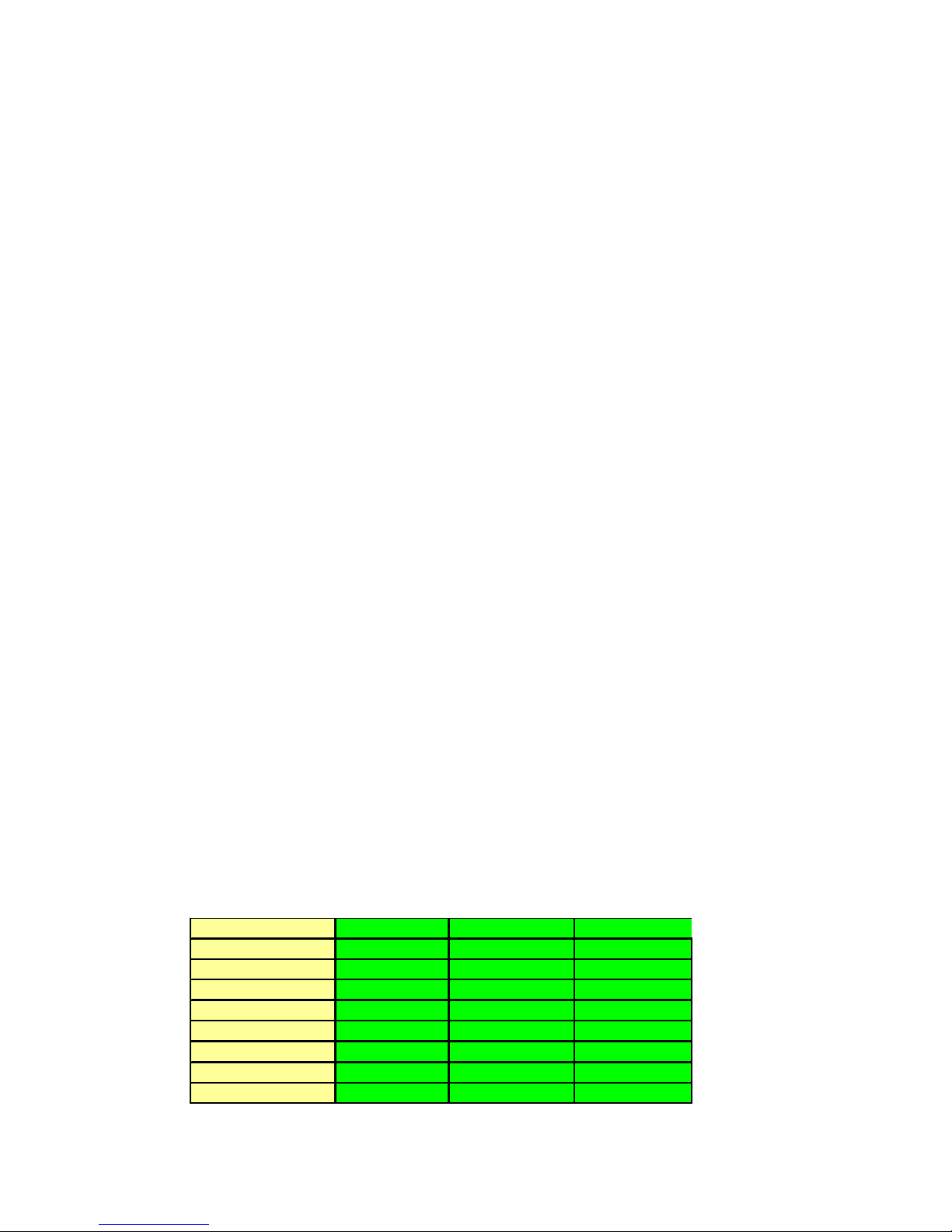
Conclusions:

1. The performance of each DB connection interface provides exceptional response time at very high throughput. Each order processed consisted of ten web requests. As a result, the capacity ranges from about 650 transactions per second up to about 870 transactions per second. Using Zend Platform will provide even higher performance (refer to the section on Zend Platform).

2. The i5 PHP API Toolkit is networked enabled so provides the capability to run in a 3-tier environment, ie, where the PHP application is running on web server deployed on a separate system from the backend DB server. However, when running in a 2- tier environment, it is recommended to use the ibm_db2 PHP extension to access DB2 locally given the optimized performance.

The i5 PHP API Toolkit provides a wealth of interfaces to integrate PHP pages with native i5 system services. When standardizing on the use of the i5 toolkit API, the use of the SQL functions to access DB2 will provide very good performance. In addition to SQL functions, the toolkit provides a program call interface to call existing programs. Calling existing programs using native DB IO may provide significantly more performance.

3. The most compelling reason to use MySQL on IBM i is when you are deploying an application that is written to the MySQL database.

Database - Persistent versus Non-Persistent Connections

If you're connecting to a DB2 database in your PHP application, you'll find that there are two alternative connections - db2_connect which establishes a new connection each time and db2_pconnect which uses persistent connections. The main advantage of using a persistent connection is that it avoids much of the initialization and teardown normally associated with getting a connection to the database. When db2_close() is called against a persistent connection, the call always returns TRUE, but the underlying DB2 client connection remains open and waiting to serve the next matching db2_pconnect() request.

One main area of concern with persistent connections is in the area of commitment control. You need to be very diligent when using persistent connections for transactions that require the use of commitment control boundaries. In this case, DB2_AUTOCOMMIT_OFF is specified and the programmer controls the commit points using db2_commit() statements. If not managed correctly, mixing managed commitment control and persistent connections can result in unknown transaction states if errors occur.

In the following table, we compare the performance of utilizing non-persistent connections in all cases versus using a mix of persistent and non-persistent connections versus using persistent connections in all cases.

OS / DB ZendCore Version Connect

OPM RT (ms) Total CPU CPU - Zend/AP CPU - DB

i 5.4 / DB2 i 5.4 / DB2 i 5.4 / DB2

V2.5.2 V2.5.2 V2.5.2

db2_connect Mixed db2_pconnect

445 2161 4997

2021 414 176

91 99 99

93362

78 62 33

IBM i 6.1 Performance Capabilities Reference - January/April/October 2008

Conclusions:

1. As stated earlier, persistent connections can dramatically improve overall performance. When using persistent connections for all transactions, the DB CPU utilization is significantly less than when using non-persistent connections.

2. For any transactions that run with autocommit turned on, use persistent connections. If the transaction requires that autocommit be turned off, use of non-persistent connections may be sufficient for pages that don’t have heavy usage. However, if a page is heavily used, use of persistent connections may be required to achieve acceptable performance. In this case, you will need a well designed transaction that handles error processing to ensure no commits are left outstanding.

Database - Isolation Levels

Because the transaction isolation level determines how data is locked and isolated from other processes while the data is being accessed, you should select an isolation level that balances the requirements of concurrency and data integrity. DB2_I5_TXN_SERIALIZABLE is the most restrictive and protected transaction isolation level, and it incurs significant overhead. Many workloads do not require this level of isolation protection. We did limited testing comparing the performance of using DB2_I5_TXN_READ_COMMITTED versus DB2_I5_TXN_READ_UNCOMMITTED isolation levels. With this workload, running under DB2_I5_TXN_READ_COMMITTED reduced the overall capacity by about 5%. However a given application might never update the underlying data or run with other concurrent updaters and DB2_I5_TXN_READ_UNCOMMITTED may be sufficient. Therefore, review your isolation level requirements and adjust them appropriately.

Zend Platform

Zend Platform for i is the production environment that ensures PHP applications are always available, fast, reliable and scalable on the i platform. Zend Platform provides caching and optimization of compiled PHP code, which provides significant performance improvement and scalability. Other features of Zend Platform that brings additional value, include:

y 5020 Bridge – API for accessing 5250 data streams

which allows Web front ends to be created

for existing applications.

y PHP Intelligence – provides monitoring of PHP applications and captures all the information

needed to pinpoint the root cause of problems and performance bottlenecks

y Online debugging and immediate error resolution with Zend Studio for i y PHP/Java integration bridge

By automatically caching and optimizing the compiled PHP code, application response time and system capacity improves dramatically. The best part for this is that no changes are required to the take advantage of this optimization. In the measurements included below, the default Zend Platform settings were used.

IBM i 6.1 Performance Capabilities Reference - January/April/October 2008

OS / DB Zend Version Connect

i 6.1 / DB2 i 6.1/MySQL 5.0

V2.5.2 V2.5.2/Platform V2.5.2 V2.5.2/Platform

db2_pconnect db2_pconnect mysqli mysqli

OPM RT (ms) Total CPU CPU - Zend/AP CPU - DB

5041 6795 3974 4610

176 129 224 191

98 95 98 96 62 44 49 31 31 46 47 62

Conclusions:

1. In both cases above, the overall system capacity improved significantly when using Zend Platform, by about 15-35% for this workload. With each order consisting of 10 web requests, processing 6795 orders per minute translates into about 1132 transactions per second.

2. Zend Platform will reduce the amount of processing in the Zend Core component since the PHP code is compiled once and reused. In both of the above cases, the amount of processing done in Zend Core on a per transaction basis was dramatically reduced by a factor of about 1.9X.

PHP System Sizing

The IBM Systems Workload Estimator (a.k.a., the Estimator or WLE) is a web-based sizing tool for IBM Power Systems, System i, System p, and System x. You can use this tool to size a new system, to size an upgrade to an existing system, or to size a consolidation of several systems. The Estimator allows measurement input to best reflect your current workload and provides a variety of built-in workloads to reflect your emerging application requirements.

Currently, a new built-in workload is being developed to allow the sizing of PHP workloads on Power Systems running IBM i. This built-in is expected to be available November 2008. To access WLE use the following URL:

http://www.ibm.com/eserver/iseries/support/estimator

IBM i 6.1 Performance Capabilities Reference - January/April/October 2008

6.3 WebSphere Application Server

This section discusses System i performance information for the WebSphere Application Server, including WebSphere Application Server V6.1, WebSphere Application Server V6.0, WebSphere Application Server V5.0 and V5.1, and WebSphere Application Server Express V5.1. Historically, both WebSphere and i5/OS Java performance improve with each version. Note from the figures and data in this section that the most recent versions of WebSphere and/or i5/OS generally provides the best performance.

What’s new in V6R1?

The release of i5/OS V6R1 brings with it significant performance benefits for many WebSphere applications. The following chart shows the amount of improvement in transactions per second (TPS) for the Trade 6.1 workload using various data access methods:

V5R4 GA V6R1 GA

1400 1200 1000

+68% +78%

+50%

800 600 400 200

Thi

Native JDBC Toolbox JDBC Universal JCC

ws that in V6R1, throughput levels for Trade 6.1 increased from 50% to nearly 80% versus V5R4, depending on which JDBC provider was being used. All measurement results were obtained in a 2-tier environment (both application and database on the same partition) on a 2-core 2.2Ghz System i partition, using Version 6.1 of WebSphere Application Server and IBM Technology for Java VM. Although many of the improvements are applicable to 3-tier environments as well, the communications overhead in these environments may affect the amount of improvement that you will see.

s cha rt sho

The improvements in V6R1 were primarily in the JDBC, DB2 for i5/OS and Java areas, as well as changes in other i5/OS components such as seize/release and PASE call overhead. The majority of the improvements will be achieved without any changes to your application, although some improvements do require additional tuning (discussed below in Tuning Changes for V6R1). Although some of the changes are now available via V5R4 PTFs, the majority of the improvement will only be realized by moving to V6R1. The actual amount of improvement in any particular application will vary, particularly depending on the amount of JDBC/DB activity, where a significant majority of the changes were made. In addition,

IBM i 6.1 Performance Capabilities Reference - January/April/October 2008

because the improvements largely resulted from significant reductions in pathlength and CPU, environments that are constrained by other resources such as IO or memory may not show the same level of improvements seen here.

Tuning changes in V6R1

As indicated above, most improvements will require no changes to an application. However, there are a few changes that will require some tuning in order to be realized:

y Using direct map (native JDBC)

For System i, the JDBC interfaces run more efficiently if direct mapping of data is used, where the data being retrieved is in a form that closely matches how the data is stored in the database files. In V6R1, significant enhancements were made in JDBC to allow direct map to be used in more cases. For the toolbox and JCC JDBC drivers, where direct map is the default, there is no change needed to realize these gains. However, for native JDBC, you will need to use the “directMap=true” custom property for the datasource in order to maximize the gain from these changes. For Trade 6.1, measurements show that adding this property results in about a 3-5% improvement in throughput. Note that there is no detrimental effect from using this property, since the JDBC interfaces will only use direct map if it is functionally viable to do

so.

y Use of unix sockets (toolbox JDBC)

For toolbox JDBC, the default is to use TCP/IP inet sockets for requests between the application server and the database connections. In V6R1, an enhancement was added to allow the use of unix sockets in a 2-tier toolbox environment (application and database reside on the same partition). Using unix sockets for the Trade 6.1 2-tier workload in V6R1 resulted in about an 8-10% improvement in throughput. However, as the default is still to use inet sockets, you will need to ensure that the class path specified in the JDBC provider is set to use the jt400native.jar file (not the jt400.jar file) in order to use unix sockets. Note that the improvement is applicable only to 2-tier toolbox environments. Inet sockets will continue to be used for all other multiple tier toolbox environments no matter which .jar file is used. .

y Using ‘threadUsed=false” custom property (toolbox JDBC)

In toolbox JDBC, the default method of operation is to use multiple application server threads for each request to a database connection, with one thread used for sending data to the connection and another thread being used to receive data from the connection. In V6R1, changes were made to allow both the send and receive activity to be done within a single application server thread for each request, thus reducing the overhead associated with the multiple threads. To gain the potential improvement from this change, you will need to specify the “threadUsed=false” custom property in the toolbox datasource, since the default is still to use multiple threads. For the Trade 6.1 workload, use of the this property resulted in about a 10% improvement in throughput.

Tuning for WebSphere is important to achieve optimal performance. Please refer to the WebSphere Application Server for iSeries Performance Considerations or the WebSphere Info Center documents for

more information. These documents describe the performance differences between the different WebSphere Application Server versions on the System i platform. They also contain many performance recommendations for environments using servlets, Java Server Pages (JSPs), and Enterprise Java Beans.

IBM i 6.1 Performance Capabilities Reference - January/April/October 2008

For WebSphere 5.1 and earlier refer to the Performance Considerations guide at:

www.ibm.com/servers/eserver/iseries/software/websphere/wsappserver/product/PerformanceConsideratio ns.html

For WebSphere 5.1, 6.0 and 6.1 please refer to the following page and follow the appropriate link:

ww.ibm.com/software/webservers/appserv/was/library/

Although some capacity planning information is included in these documents, please use the IBM Systems Workload Estimator as the primary tool to size WebSphere environments. The Workload Estimator is kept up to date with the latest capacity planning information available.

IBM i 6.1 Performance Capabilities Reference - January/April/October 2008

Trade 6 Benchmark (IBM Trade Performance Benchmark Sample for WebSphere Application Server) Description:

Trade 6 is the fourth generation of the WebSphere end-to-end benchmark and performance sample application. The Trade benchmark is designed and developed to cover the significantly expanding programming model and performance technologies associated with WebSphere Application Server. This application provides a real-world workload, enabling performance research and verification test of the

2 Platform, Enterprise Edition (J2EETM) 1.4 implementation in WebSphere Application Server,

Java including key performance components and features.

Overall, the Trade application is primarily used for performance research on a wide range of software components and platforms. This latest revision of Trade builds off of Trade 3, by moving from the J2EE

1.3 programming model to the J2EE 1.4 model that is supported by WebSphere Application Server V6.0. Trade 6 adds DistributedMap based data caching in addition to the command bean caching that is used in Trade 3. Otherwise, the implementation and workflow of the Trade application remains unchanged.

Trade 6 also supports the recent DB2® V8.2 and Oracle® 10g databases. The new design of Trade 6

enables performance research on J2EE 1.4 including the new Enterprise JavaBeansTM (EJB

) 2.1 component architecture, message-driven beans, transactions (1-phase, 2-phase commit) and Web services (SOAP, WSDL, JAX-RPC, enterprise Web services). Trade 6 also drives key WebSphere Application Server performance components such as dynamic caching, WebSphere Edge Server, and EJB caching.

NOTE: Trade 6 is an updated version of Trade 3 which takes advantage of the new JMS messaging support available with WebSphere 6.0. The application itself is essentially the same as Trade 3 so direct comparisons can be made between Trade 6 and Trade 3. However, it is important to note that direct comparisons between Trade2 and Trade3 are NOT valid. As a result of the redesign and additional components that were added to Trade 3, Trade 3 is more complex and is a heavier application than the previous Trade 2 versions.

Figure 6. 1 Topology of the Trade Application

IBM i 6.1 Performance Capabilities Reference - January/April/October 2008

The Trade 6 application allows a user, typically using a Web browser, to perform the following actions:

y Register to create a user profile, user ID/password and initial account balance y Login to validate an already registered user y Browse current stock price for a ticker symbol y Purchase shares y Sell shares from holdings y Browse portfolio y Logout to terminate the users active interval

Each action is comprised of many primitive operations running within the context of a single HTTP request/response. For any given action there is exactly one transaction comprised of 2-5 remote method calls. A Sell action for example, would involve the following primitive operations:

y Browser issues an HTTP GET command on the TradeAppServlet y TradeServlet accesses the cookie-based HTTP Session for that user y HTML form data input is accessed to select the stock to sell y The stock is sold by invoking the sell() method on the Trade bean, a stateless Session EJB. To

achieve the sell, a transaction is opened and the Trade bean then calls methods on Quote, Account and Holdings Entity EJBs to execute the sell as a single transaction.

y The results of the transaction, including the new current balance, total sell price and other data,

are formatted as HTML output using a Java Server Page, portfolio.jsp.

y Message Driven Beans are used to inform the user that the transaction has completed on the next

logon of that user.

To measure performance across various configuration options, the Trade 6 application can be run in several modes. A mode defines the environment and component used in a test and is configured by modifying settings through the Trade 6 interface. For example, data object access can be configured to use JDBC directly or to use EJBs under WebSphere by setting the Trade 6 runtime mode. In the Sell example above, operations are listed for the EJB runtime mode. If the mode is set to JDBC, the sell action is completed by direct data access through JDBC from the TradeAppServlet. Several testing modes are available and are varied for individual tests to analyze performance characteristics under various configurations.

IBM i 6.1 Performance Capabilities Reference - January/April/October 2008

WebSphere Application Server V6.1

Historically, new releases of WebSphere Application Server have offered improved performance and functionality over prior releases of WebSphere. WebSphere Application Server V6.1 is no exception. Furthermore, the availability of WebSphere Application Server V6.1 offers an entirely new opportunity for WebSphere customers. Applications running on V6.1 can now operate with either the “Classic” 64-bit Virtual Machine (VM) or the recently released IBM Technology for Java, a 32-bit VM that is built on technology being introduced across all the IBM Systems platforms.

Customers running releases of WebSphere Application prior to V6.1 will likely be familiar with the Classic 64-bit VM. This continues to be the default VM on i5/OS, offering competitive performance and excellent vertical scalability. Experiments conducted using the Trade6 benchmark show that WebSphere Application Server V6.1 running on the Classic VM realized performance gains of 5-10% better throughput when compared to WebSphere Application Server V6.0 on identical hardware.

In addition to the presence of the Classic 64-bit VM, WebSphere Application Server V6.1 can also take advantage of IBM Technology for Java, a 32-bit implementation of Java supported on Java 5.0 (JDK 1.5). For V6.1 users, IBM Technology for Java has two key potentially beneficial characteristics:

y Significant performance improvements for many applications - Most applications will see at least equivalent performance when comparing WebSphere Application Server on the Classic VM to IBM Technology for Java, with many applications seeing improvements of up to 20%. y 32-bit addressing allows for a potentially considerable reduction in memory footprint - Object references require only 4 bytes of memory as opposed to the 8 bytes required in the 64-bit Classic VM. For users running on small systems with relatively low memory demands this could offer a substantially smaller memory footprint. Performance tests have shown approximately 40% smaller Java Heap sizes when using IBM Technology for Java when compared to the Classic VM.

It is important to realize that both the Classic VM and IBM Technology for Java have excellent benefits for different applications. Therefore, choosing which VM to use is an extremely important consideration. Chapter 7 - Java Performance has an extensive overview of many of the key decisions that go into choosing which VM to use for a given application. Most of the points in Chapter 7 are very much important to WebSphere Application Server users. One issue that will likely not be a concern to WebSphere Application Server users is the additional overhead to native ILE calls that is seen in IBM Technology for Java. However, if native calls are relevant to a particular application, that consideration will of course be important. While choosing the appropriate VM is important, WebSphere Application Server V6.1 allows users to toggle between the Classic VM and IBM Technology for Java either for the entire WebSphere installation or for individual application server profiles.

While 32-bit addressing can provide smaller memory footprints for some applications, it is imperative to understand the other end of the spectrum: applications requiring large Java heaps may not be able to fit in the space available to a 32-bit implementation of Java. The 32-bit VM has a maximum heap size of 3328 MB for Java applications. However, WebSphere Application Server V6.1 using IBM Technology for Java has a practical maximum heap size of around 2500 MB due in part to WebSphere related memory demands like shared classes. The Classic VM should be used for applications that require a heap larger than 2500 MB (see Chapter 7 - Java Performance for further details).

IBM i 6.1 Performance Capabilities Reference - January/April/October 2008

Trade3 Measurement Results:

Trade on S ystem i - H istorical V iew

550 500 450 400 350 300 250 200 150

Transactions/Second

100

Trade3-EJB Trade3-JDBC

V5R2 WAS 5.0 V5R3 WAS 5.0

V5R3 WAS 5.1 V5R3 WAS 6.0 (Trade6)

Capacity

Trade 3/6 on model 825 2 Way LP AR

V5R4 WAS 6.0 (Trade6) V5R4 WAS 6.1 Classic (Trade 6.1)

V5R4 WAS 6.1 IBM Tech For Java (Trade 6.1)

Figure 6.2 Trade Capacity Results

WebSphere Application Server Trade Results

Notes/Disclaimers:

y Trade3 chart: WebSphere 5.0 was measured on both V5R2 and V5R3 on a 4 way (LPAR) 825/2473 system WebSphere 5.1 was measured on V5R3 on a 4 way (LPAR) 825/2473 system WebSphere 6.0 was measured on V5R3 on a 4 way (LPAR) 825/2473 system WebSphere 6.0 was measured on V5R4 on a 2 way (LPAR) 570/7758 system WebSphere 6.1 using Classic VM was measured on V5R4 on a 2 way (LPAR) 570/7758 system WebSphere 6.1 using IBM Technology for Java was measured on V5R4 on a 2 way (LPAR) 570/7758 system

IBM i 6.1 Performance Capabilities Reference - January/April/October 2008

Trade Scalability Results:

Trade on System i

Scaling of Hardware and Software

T rade 3

4000

3500

3000

2500

2000

1500

Transactions/Second

1000

500

V5R2 WAS 5.0 V5R2 WAS 5.1 V5R3 WAS 5.1

EJB JDBC

Transactions/Second

1200

1000

800

600

400

200

Power 5

EJB JDBC

Power4 2 Way (LPAR) 1.1 Ghz Power5 2 Way 1.65 Ghz Power5 2 way (LPAR) 2.2 Ghz

2000

1500

1000

Transactions/Second

500

Power 6

EJB JDBC

Power5 2 way (LPAR) 2.2 Ghz Power6 2 way (LPAR) 4.6 Ghz

Figure 6.3 Trade Scaling Results

WebSphere Application Server Trade Results

Notes/Disclaimers:

y Trade 3 chart:

V5R2 - 890/2488 32-Way 1.3 GHz, V5R2 was measured with WebSphere 5.0 and WebSphere 5.1 V5R3 - 890/2488 32-Way 1.3 GHz, V5R3 was measured with WebSphere 5.1 POWER5 chart: POWER4 - V5R3 825/2473 2-Way (LPAR) 1.1 GHz., Power4 was measured with WebSphere 5.1 POWER5 - V5R3 520/7457 2-Way 1.65 GHz., Power5 was measured with WebSphere 5.1

POWER5 - V5R4 570/7758 2-Way (LPAR) 2.2 GHz, Power5 was measured with WebSphere 6.0 y POWER6 chart: POWER5 - V5R4 570/7758 2-Way (LPAR) 2.2 GHz, Power5 was measured with WebSphere 6.0 POWER6 - V5R4 9406-MMA 2-Way (LPAR) 4.7 GHz, Power6 was measured with WebSphere 6.1

Trade 6 Primitives

Trade 6 provides an expanded suite of Web primitives, which singularly test key operations in the enterprise Java programming model. These primitives are very useful in the Rochester lab for

release-to-release

comparison tests, to determine if a degradation occurs between releases, and what areas to target performance improvements. Table 6.1 describes all of the primitives that are shipped with Trade 6, and Figure 6.4 shows the results of the primitives from WAS 5.0 and WAS 5.1. In V5R4 a few of the primitives were tracked on WAS 6.0, showing a change of 0-2%, the results of which are not included in Figure 6.4. In the future, additional primitives are planned again to be measured for comparison.

IBM i 6.1 Performance Capabilities Reference - January/April/October 2008

IBM 170 Servers, 7xx Servers, AS/400 RISC Server User Manual

Specifications and Main Features

Frequently Asked Questions

User Manual