

Page 1

SG24-4895-00
AS/400 Communication Performance Investigation
- V3R6/V3R7
December 1997
Page 2

Page 3

IBML
International Technical Support Organization
SG24-4895-00
AS/400 Communication Performance Investigation
- V3R6/V3R7
December 1997
Page 4

Take Note!
Before using this information and the product it supports, be sure to read the general information in
Appendix J, “Special Notices” on page 389.
First Edition (December 1997)
This edition applies to Version 3, Release 7, Modification 0 of the AS/400 Operating System and to all subsequent
releases until otherwise indicated in new editions or technical bulletins.
Comments may be addressed to:
IBM Corporation, International Technical Support Organization
Dept. JLU Building 107-2
3605 Highway 52N
Rochester, Minnesota 55901-7829
When you send information to IBM, you grant IBM a non-exclusive right to use or distribute the information in any
way it believes appropriate without incurring any obligation to you.
Copyright International Business Machines Corporation 1997. All rights reserved.
Note to U.S. Government Users — Documentation related to restricted rights — Use, duplication or disclosure is
subject to restrictions set forth in GSA ADP Schedule Contract with IBM Corp.
Page 5

Contents
Preface . . . . . . . . . . . . . . . . . . . . . . . . . . . . . . . . . . . . . . . . . . xi
The Team That Wrote This Redbook
Comments Welcome
. . . . . . . . . . . . . . . . . . . . . . . . . . . . . . . . . . xii
......................... xi
Chapter 1. Tools Used for Finding Performance Problems
1.1 Usual Symptoms of Degraded Performance
1.2 Collecting Communications Performance Data
1.2.1 Why Collect Performance Data
....................... 3
1.2.2 How to Collect Performance Data
1.2.3 Automatic Data Collection
1.2.4 Performance Management/400
1.3 Using CL Commands Interactively
1.4 Using Performance Tools/400
1.4.1 WRKSYSACT Command
1.4.2 PRTACTRPT Command
1.4.3 DSPPFRDTA Command
1.4.4 The A dvisor
1.4.5 Produce Reports
1.5 What to Look For
. . . . . . . . . . . . . . . . . . . . . . . . . . . . . . . . . . 7
................................ 7
.................................. 8
.......................... 5
. . . . . . . . . . . . . . . . . . . . . . . 5
........................ 6
.......................... 6
. . . . . . . . . . . . . . . . . . . . . . . . . . . 6
. . . . . . . . . . . . . . . . . . . . . . . . . . . 7
. . . . . . . . . . . . . . . . . . . . . . . . . . . 7
.................. 2
................ 2
..................... 3
........... 1
Chapter 2. Using CL Commands to Find Performance Problems
2.1 WRKSYSVAL Command
2.1.1 QTOTJOB
2.1.2 QACTJOB
. . . . . . . . . . . . . . . . . . . . . . . . . . . . . . . . . . . . 11
. . . . . . . . . . . . . . . . . . . . . . . . . . . . . . . . . . . . 12
2.1.3 QMAXACTLVL
2.1.4 QMCHPOOL
2.1.5 QCMNRCYLMT
2.2 PRTERRLOG Command
2.3 PTF Commands
2.3.1 DSPPTF
. . . . . . . . . . . . . . . . . . . . . . . . . . . . . . . . . . . 14
. . . . . . . . . . . . . . . . . . . . . . . . . . . . . . . . . . . . . 15
2.3.2 SNDPTFORD
2.4 WRKSYSSTS Command
2.4.1 WRKSYSSTS
2.4.2 Information About Activity Level Guidelines
2.4.3 Information About Transition Guidelines
2.4.4 Interactive Tuning Roadmap
2.5 WRKACTJOB Command
2.6 Using WRKDSKSTS
2.7 WRKSYSACT Command
. . . . . . . . . . . . . . . . . . . . . . . . . . . . . . 11
.................................12
. . . . . . . . . . . . . . . . . . . . . . . . . . . . . . . . . . 13
. . . . . . . . . . . . . . . . . . . . . . . . . . . . . . . . 13
. . . . . . . . . . . . . . . . . . . . . . . . . . . . . . 14
. . . . . . . . . . . . . . . . . . . . . . . . . . . . . . . . . . 15
. . . . . . . . . . . . . . . . . . . . . . . . . . . . . . 16
. . . . . . . . . . . . . . . . . . . . . . . . . . . . . . . . . . 16
............... 19
................. 19
........................ 20
. . . . . . . . . . . . . . . . . . . . . . . . . . . . . . 21
. . . . . . . . . . . . . . . . . . . . . . . . . . . . . . . . 23
. . . . . . . . . . . . . . . . . . . . . . . . . . . . . . 24
........ 11
Chapter 3. Using Performance Tools/400
3.1 System-Wide Problem Analysis
3.1.1 A dvisor
3.1.2 Performance Graphics
3.1.3 Print Activity Report
. . . . . . . . . . . . . . . . . . . . . . . . . . . . . . . . . . . . . 27
. . . . . . . . . . . . . . . . . . . . . . . . . . . . 29
............................. 30
3.1.4 Performance Tools Reports
3.1.5 Memory Performance Displays and Reports
3.1.6 CPU Performance Reports and Displays
3.1.7 A Brief Discussion About Program Exceptions Consuming CPU
3.1.8 D isk Performance Reports and Displays
3.1.9 Communications Performance Data
Copyright IBM Corp. 1997 iii
...................... 27
......................... 27
......................... 31
............... 33
................. 34
... 34
................. 37
.................... 39
Page 6

3.1.10 Activity Level Performance Reports and Displays ........... 41
3.1.11 Comparing with Activity Level Guidelines
3.1.12 Comparing W-I and A-W Ratio Guidelines
3.2 User Level Problem Analysis
3.2.1 Print Job Summary Report
........................... 42
......................... 43
3.2.2 P rin t Tr ansaction Summary Report
3.3 Application Level Problem Analysis
....................... 43
3.3.1 Charging Resource Utilization to Interactive Program
3.3.2 P rin t Tr ansaction Summary Report
3.3.3 Print Transaction Detail Report
3.3.4 Print Transition Report
............................ 45
3.4 Programmer Performance Utilities
3.4.1 O S/ 400 Utilities for Tracing a Job
....................... 44
....................... 46
..................... 46
3.4.2 Performance Tools/400 Utilities for Tracing a Job
3.5 Performance Data Conversion
.......................... 51
................ 42
................ 42
.................... 43
......... 44
.................... 44
............ 48
Chapter 4. Using BEST/1 for Communications Performance Analysis and
Capacity Planning . . . . . . . . . . . . . . . . . . . . . . . . . . . . . . . . . . . 53
4.1 V3R7 BEST/1 Capacity Planning
4.1.1 When to Use BEST/1 for Communications Performance Analysis
4.2 Creating a Model for Communications Analysis
4.2.1 Assigning Jobs to Workloads by Communications Line
4.2.2 Creating a Model
............................... 58
4.3 Using a Model for Communications Analysis
4.3.1 Displaying Model Reports
4.3.2 Understanding Recommendations
4.4 Changing Communications Resources
4.4.1 Example - Changing the IOP Type
4.5 BEST/1 Communications Support for Performance Analysis
4.5.1 Creating a Communications IOP Feature
4.5.2 Creating a Communications Line Resource
4.5.3 Distribution of Characters Transferred Across Line Resources
4.6 Comparing the Model Against the Measured Performance
4.7 Considerations When Analyzing Communications Data with BEST/1
......................... 53
.. 53
............... 54
........ 54
................. 58
.......................... 58
. . . . . . . . . . . . . . . . . . . . . 59
..................... 62
..................... 64
........ 65
................. 65
............... 67
.... 68
......... 69
... 70
Chapter 5. Using System Service Tools
5.1 Checking the Communications Hardware
5.2 Working with Communications Traces
5.2.1 Starting and Stopping the Trace
5.2.2 Formatting the Trace Data
Chapter 6. Communications I/O Processor (IOP)
6.1 Important Fields in the IOP Performance Manager File
6.1.1 I OP Utilization
6.2 Communication IOP Recommendations
6.2.1 Configuring Communication Lines
6.2.2 Frame Size
6.2.3 IOP Type
6.2.4 IOP Assist
6.2.5 IOP Utilization
Chapter 7. Local Area Network Performance Analysis
7.1 LAN Performance Indicators in Performance Monitor Database
7.2 Line Utilization
7.2.1 Using Performance Tools/400 to Display Line Utilization
iv Comm Perf Investigation - V3R6/V3R7
....................... 71
................... 71
..................... 80
...................... 80
.......................... 84
................. 89
........... 89
. . . . . . . . . . . . . . . . . . . . . . . . . . . . . . . . . 89
.................... 92
..................... 93
. . . . . . . . . . . . . . . . . . . . . . . . . . . . . . . . . . . 94
. . . . . . . . . . . . . . . . . . . . . . . . . . . . . . . . . . . . 94
. . . . . . . . . . . . . . . . . . . . . . . . . . . . . . . . . . . 95
. . . . . . . . . . . . . . . . . . . . . . . . . . . . . . . . . 95
.............. 97
...... 97
. . . . . . . . . . . . . . . . . . . . . . . . . . . . . . . . . . . 97
........ 97
Page 7

7.2.2 Performance Monitor Database Fields .................. 99
7.2.3 Recommendations
7.3 LAN Congestion
.................................. 100
7.3.1 Not Ready and Sequence Errors
7.3.2 Using Performance Tools/400 to Display Congestion
7.3.3 Performance Monitor Database Fields
7.3.4 Receive Congestion Errors on Token-Rings
7.3.5 Ethernet Collision Counters
7.3.6 Recommendations to Control Congestion
7.4 Medium Access Control (MAC) Errors
7.4.1 Using Performance Tools/400 to Display MAC Errors
7.4.2 Performance Monitor Database Fields
7.4.3 Recommendations
7.4.4 T oke n-R ing Net work Errors
7.5 Retransmissions
7.6 Timeouts
. . . . . . . . . . . . . . . . . . . . . . . . . . . . . . . . . . . . . . 111
7.6.1 Using Performance Tools/400 to Display Timeouts and Retries
7.6.2 Performance Monitor Database Fields
7.7 LAN Overheads
. . . . . . . . . . . . . . . . . . . . . . . . . . . . . . . . . . 113
7.7.1 Performance Monitor Database Fields
7.8 LAN Queries
. . . . . . . . . . . . . . . . . . . . . . . . . . . . . . . . . . . . 115
7.9 LAN Performance Tuning Recommendations
7.9.1 LAN Controller Performance Parameters
7.9.2 LANCNNTMR and LANCNNRTY
7.9.3 LANRSPTMR and LANFRMRTY
7.9.4 LANACKTMR and LANACKFRQ
7.9.5 LANACKTMR and LANRSPTMR Relationship
7.9.6 LANACKFRQ and LANMAXOUT Relationship
7.9.7 LANINACTMR
7.9.8 LANWDWSTP
7.9.9 LANACCPTY (Token-Ring Networks Only)
7.10 L A N IOPs
7.11 Frame Size
. . . . . . . . . . . . . . . . . . . . . . . . . . . . . . . . . . . . . 122
. . . . . . . . . . . . . . . . . . . . . . . . . . . . . . . . . . . . 124
7.11.1 Token-Ring Frame Sizes
7.11.2 Ethernet Frame Sizes
7.11.3 Bridge Frame Size Considerations
7.11.4 ETHSTD Parameter
7.11.5 Other Considerations
. . . . . . . . . . . . . . . . . . . . . . . . . . . . . 100
..................... 101
......... 101
................. 102
.............. 104
........................ 104
................ 105
.................... 106
......... 106
................. 107
. . . . . . . . . . . . . . . . . . . . . . . . . . . . . 109
........................ 110
. . . . . . . . . . . . . . . . . . . . . . . . . . . . . . . . . 110
... 111
................. 112
................. 114
................ 115
................ 115
...................... 116
...................... 117
..................... 118
............. 118
............. 120
. . . . . . . . . . . . . . . . . . . . . . . . . . . . . . . . 121
. . . . . . . . . . . . . . . . . . . . . . . . . . . . . . . . . 121
............... 122
......................... 124
........................... 124
................... 125
. . . . . . . . . . . . . . . . . . . . . . . . . . . . 126
. . . . . . . . . . . . . . . . . . . . . . . . . . . 126
Chapter 8. X.25
8.1 High Level Data Link Control (HDLC)
8.1.1 Line Utilization
8.1.2 Line Errors
8.1.3 Congestion
8.1.4 Data Link Resets
8.2 Packet level Control (PLC)
8.2.1 Number of Packets Transmitted
8.2.2 Congestion
8.3 Logical Link Control (LLC)
. . . . . . . . . . . . . . . . . . . . . . . . . . . . . . . . . . . . 127
..................... 127
. . . . . . . . . . . . . . . . . . . . . . . . . . . . . . . . 128
. . . . . . . . . . . . . . . . . . . . . . . . . . . . . . . . . . 131
. . . . . . . . . . . . . . . . . . . . . . . . . . . . . . . . . . 133
.............................. 135
........................... 136
..................... 136
. . . . . . . . . . . . . . . . . . . . . . . . . . . . . . . . . . 137
........................... 137
8.3.1 Data Units Retransmitted and Data Units Received in Error
8.3.2 L LC Rejects
8.3.3 LLC Protocol Data Units Discarded
8.3.4 Timeouts
8.3.5 Checksum Errors Detected
. . . . . . . . . . . . . . . . . . . . . . . . . . . . . . . . . 139
................... 140
. . . . . . . . . . . . . . . . . . . . . . . . . . . . . . . . . . . 141
........................ 141
8.3.6 Number of Reset Indications from Packet Link Control
..... 138
........ 142
Contents v
Page 8

8.3.7 LLC Congestion . . . . . . . . . . . . . . . . . . . . . . . . . . . . . . . 142
8.4 Important Related Performance Manager Files
8.4.1 I OP Utilization
8.4.2 Remote Jobs
. . . . . . . . . . . . . . . . . . . . . . . . . . . . . . . . 143
. . . . . . . . . . . . . . . . . . . . . . . . . . . . . . . . . 144
............... 143
Chapter 9. SDLC
. . . . . . . . . . . . . . . . . . . . . . . . . . . . . . . . . . . 147
9.1 Important Fields in the SDLC Performance Manager File
9.1.1 Line Utilization
9.1.2 Line Errors
9.1.3 Congestion
9.1.4 Data Link Resets
9.1.5 Connect Poll Retries
9.2 Other Related Performance Monitor Files
9.2.1 I OP Utilization
9.2.2 Remote Jobs
Chapter 10. SNA
. . . . . . . . . . . . . . . . . . . . . . . . . . . . . . . . 147
. . . . . . . . . . . . . . . . . . . . . . . . . . . . . . . . . . 150
. . . . . . . . . . . . . . . . . . . . . . . . . . . . . . . . . . 153
.............................. 155
............................ 155
.................. 158
. . . . . . . . . . . . . . . . . . . . . . . . . . . . . . . . 159
. . . . . . . . . . . . . . . . . . . . . . . . . . . . . . . . . 160
. . . . . . . . . . . . . . . . . . . . . . . . . . . . . . . . . . . . 163
10.1 Important Fields in the SNA Performance Monitor File
10.1.1 Number of Connections Established
.................. 164
10.1.2 Number of Sessions and Brackets Started/Ended
10.1.3 Session Level Pacing Wait Time
10.1.4 Internal Session Level Pacing
10.1.5 Transmission Queue Wait Time
10.1.6 Line Transmission Time
......................... 169
10.2 Important Related Performance Manager Files
10.2.1 Line Utilization
10.2.2 Communications Jobs
10.3 SNA Traces
.................................... 173
. . . . . . . . . . . . . . . . . . . . . . . . . . . . . . . 171
. . . . . . . . . . . . . . . . . . . . . . . . . . . 172
.................... 166
...................... 167
..................... 168
.............. 170
......... 147
.......... 163
.......... 165
Chapter 11. TCP/IP Performance Investigation
11.1 Performance Expectation
11.2 TCP/IP Overview
11.2.1 Data Format
11.2.2 Flow Control
. . . . . . . . . . . . . . . . . . . . . . . . . . . . . . . . 175
. . . . . . . . . . . . . . . . . . . . . . . . . . . . . . . . . 175
. . . . . . . . . . . . . . . . . . . . . . . . . . . . . . . . 176
. . . . . . . . . . . . . . . . . . . . . . . . . . . 175
11.2.3 Version 3 Performance Improvements
11.3 Performance Tool/400 Databases
11.3.1 QAPMSAP
11.3.2 QAPMJOBS
11.4 Bottlenecks
. . . . . . . . . . . . . . . . . . . . . . . . . . . . . . . . . . 177
. . . . . . . . . . . . . . . . . . . . . . . . . . . . . . . . . 178
. . . . . . . . . . . . . . . . . . . . . . . . . . . . . . . . . . . . 178
11.5 Tools We Can Use for TCP/IP
...................... 177
......................... 178
................. 175
................. 177
Chapter 12. Analyzing APPN Communications Performance
12.1 Advanced Peer-to-Peer Networking (APPN) Performance
12.1.1 APPN System Tasks
12.1.2 QLUS Task
. . . . . . . . . . . . . . . . . . . . . . . . . . . . . . . . . 183
12.1.3 Topology Maintenance
12.1.4 Directory Services Registrations and Deletions
12.1.5 Configuration Changes
............................ 182
. . . . . . . . . . . . . . . . . . . . . . . . . . 184
........... 188
. . . . . . . . . . . . . . . . . . . . . . . . . . 188
12.1.6 Control Point Session Activation and Deactivation
12.1.7 Control Point Presentation Services (CPPS)
12.1.8 Session Setup Activities
12.2 APPN Transmission Priority
......................... 192
.......................... 195
............. 190
......... 181
........ 181
.......... 190
Chapter 13. AnyNet
13.1 MPTN Architecture
vi Comm Perf Investigation - V3R6/V3R7
. . . . . . . . . . . . . . . . . . . . . . . . . . . . . . . . . . 197
. . . . . . . . . . . . . . . . . . . . . . . . . . . . . . . 197
Page 9

13.2 Types of MPTN Nodes ............................. 197
13.2.2 AnyNet
13.2.3 AnyNet/400 Summary
13.3 AnyNet Performance Considerations
13.3.1 Some Guidelines for Performance Analysis
13.3.2 AnyNet Summary
. . . . . . . . . . . . . . . . . . . . . . . . . . . . . . . . . . . . 198
. . . . . . . . . . . . . . . . . . . . . . . . . . . 198
.................... 199
.............. 200
. . . . . . . . . . . . . . . . . . . . . . . . . . . . . 205
Chapter 14. ISDN
14.1 Link Access Protocol for D-Channel (LAP-D)
14.1.1 Line Utilization (LAP-D)
14.1.2 Line Errors
14.1.3 Using Performance Tools/400 to Display Line Error Information
14.1.4 Frame Errors (LAP-D)
14.1.5 Performance Monitor Database Fields
. . . . . . . . . . . . . . . . . . . . . . . . . . . . . . . . . . . 207
................ 209
.......................... 209
. . . . . . . . . . . . . . . . . . . . . . . . . . . . . . . . . 213
.. 214
........................... 215
................. 216
14.1.6 Using Performance Tools/400 to Display Frame Error Information 217
14.1.7 Call Processing
14.1.8 Using Performance Monitor/400 to Display Call Information
14.2 ISDN Data Link Control (IDLC)
14.2.1 Line Utilization (IDLC)
14.2.2 Line Errors (IDLC)
14.2.3 Frame Errors (IDLC)
14.2.4 Using Performance Tools/400 to Display Frame Errors (IDLC)
14.3 ISDN Used with X.25 (X.31)
14.3.1 Circuit Mode
14.3.2 Packet Mode
14.3.3 Performance Monitor Database Fields
14.4 Recommendations
14.4.1 Frame Size
14.4.2 Window Size
14.4.3 Packet Size (X.25 Only)
14.4.4 A Case Study
............................... 217
.... 217
........................ 218
........................... 218
............................. 221
............................ 221
... 222
.......................... 223
. . . . . . . . . . . . . . . . . . . . . . . . . . . . . . . . 223
. . . . . . . . . . . . . . . . . . . . . . . . . . . . . . . . 224
................. 224
. . . . . . . . . . . . . . . . . . . . . . . . . . . . . . . 224
. . . . . . . . . . . . . . . . . . . . . . . . . . . . . . . . . 224
. . . . . . . . . . . . . . . . . . . . . . . . . . . . . . . . 225
.......................... 225
................................ 226
Appendix A. SDLC Queries
A.1 SDLC_ALL
A.2 SDLC_HDLC
A.3 SDLC_IOP
. . . . . . . . . . . . . . . . . . . . . . . . . . . . . . . . . . . . . 228
. . . . . . . . . . . . . . . . . . . . . . . . . . . . . . . . . . . . 231
. . . . . . . . . . . . . . . . . . . . . . . . . . . . . . . . . . . . . 233
. . . . . . . . . . . . . . . . . . . . . . . . . . . . . 227
A.3.1 IOP Query for a Communications Processor
A.3.2 I OP Query for MFIO Processor
A.4 SDLC_JOB
. . . . . . . . . . . . . . . . . . . . . . . . . . . . . . . . . . . . . 237
Appendix B. Local Area Network Queries
B.1 Token-Ring LAN Query
B.1.1 Sample Report Output
............................. 239
........................... 241
...................... 235
.................... 239
B.1.2 C L Program to Execute the Token-Ring LAN Queries
B.1.3 Token-Ring LAN SAP Counter Query
.................. 243
B.1.4 Token-Ring LAN Performance Indicators Query
B.1.5 Token-Ring LAN MAC Error Counters Query
B.1.6 Token-Ring LAN Overhead Query
B.2 Ethernet LAN Query
B.2.1 Sample Report Output
............................... 258
........................... 260
.................... 254
B.2.2 C L Program to Execute the Ethernet LAN Queries
B.2.3 Ethernet LAN SAP Counter Query
.................... 262
B.2.4 Ethernet LAN Performance Indicator Report Query
B.2.5 Ethernet LAN MAC Error Counters Query
............... 267
.............. 233
........ 242
............ 244
............. 248
.......... 261
.......... 263
Contents vii
Page 10

Appendix C. X.25 Queries . . . . . . . . . . . . . . . . . . . . . . . . . . . . . . 275
C.1 X25_ALL
C.2 X25_HDLC
C.3 X25_PLC
C.4 X25_LLC
C.5 X25_IOP
C.5.1 IOP Query for a Communications Processor
C.5.2 I OP Query for MFIO Processor
C.6 X25_JOB
. . . . . . . . . . . . . . . . . . . . . . . . . . . . . . . . . . . . . . 276
. . . . . . . . . . . . . . . . . . . . . . . . . . . . . . . . . . . . . 280
. . . . . . . . . . . . . . . . . . . . . . . . . . . . . . . . . . . . . . 282
. . . . . . . . . . . . . . . . . . . . . . . . . . . . . . . . . . . . . . 284
. . . . . . . . . . . . . . . . . . . . . . . . . . . . . . . . . . . . . . 286
.............. 286
...................... 288
. . . . . . . . . . . . . . . . . . . . . . . . . . . . . . . . . . . . . . 290
Appendix D. Queries for APPN Tasks
D.1 APPNSYSNAM Query (System Name - Input to Query APPNALL)
D.2 APPNJOIN1 Query (APPN Task - Join Input to Query APPNALL)
....................... 293
.... 295
.... 296
D.3 APPNJOIN2 Query (T2 Station IOM - Join Input to Query APPNALL)
D.4 APPNJOIN3 Query (Token-Ring IOM - Join Input to Query APPNALL)
D.5 CPUALLOC Query (System Processor Usage by Categories)
D.6 APPNALL Query (ASync Communications I/O Task Activity)
D.7 APPNDETAIL Query (APPN Tasks - Detailed Resource Usage)
D.8 APPNT2DTL Query (T2 Station IOP Task Detail)
Appendix E. SNA Queries
E.1 SNA_ALL
E.2 SNA_CON
E.3 SNA_IPAC
E.4 SNA_PAC1
E.5 SNA_PAC2
E.6 SNA_PAC3
E.7 SNA_LIN
E.8 SNA_TRQ
. . . . . . . . . . . . . . . . . . . . . . . . . . . . . . . . . . . . . . 312
. . . . . . . . . . . . . . . . . . . . . . . . . . . . . . . . . . . . . 324
. . . . . . . . . . . . . . . . . . . . . . . . . . . . . . . . . . . . . 326
. . . . . . . . . . . . . . . . . . . . . . . . . . . . . . . . . . . . . 329
. . . . . . . . . . . . . . . . . . . . . . . . . . . . . . . . . . . . . 332
. . . . . . . . . . . . . . . . . . . . . . . . . . . . . . . . . . . . . 335
. . . . . . . . . . . . . . . . . . . . . . . . . . . . . . . . . . . . . . 338
. . . . . . . . . . . . . . . . . . . . . . . . . . . . . . . . . . . . . 341
Appendix F. Integrated PC Server Query
. . . . . . . . . . . . . . . . . . . . . . . . . . . . . . 311
..................... 345
.............. 308
F.1 Integrated PC Server Performance Monitor Data Queries
Appendix G. AnyNet Queries
G.1 Sockets over SNA Queries
G.1.1 S NA Query
. . . . . . . . . . . . . . . . . . . . . . . . . . . . . . . . . . 352
G.1.2 Sockets Jobs Query
G.2 APPC over TCP/IP Queries
G.2.1 S NA Query
. . . . . . . . . . . . . . . . . . . . . . . . . . . . . . . . . . 359
G.2.2 APPC Jobs Query
. . . . . . . . . . . . . . . . . . . . . . . . . . . . 351
........................... 351
............................ 353
........................... 359
.............................. 360
...... 302
....... 304
..... 306
........ 345
.. 298
. 300
Appendix H. ISD N Queries
H.1 NWI_ALL
H.2 NWI_CALLS
H.3 NWI_ERRORS
H.4 NWI_IOP
H.5 NWI_LAPD
H.6 IDLC_ALL
H.7 IDLC_IOP
H.8 IDLC_UTIL
Appendix I. Guidelines for Interpreting Performance Data
Appendix J. Special Notices
viii Comm Perf Investigation - V3R6/V3R7
. . . . . . . . . . . . . . . . . . . . . . . . . . . . . 361
. . . . . . . . . . . . . . . . . . . . . . . . . . . . . . . . . . . . . . 362
. . . . . . . . . . . . . . . . . . . . . . . . . . . . . . . . . . . . 365
. . . . . . . . . . . . . . . . . . . . . . . . . . . . . . . . . . . 367
. . . . . . . . . . . . . . . . . . . . . . . . . . . . . . . . . . . . . . 369
. . . . . . . . . . . . . . . . . . . . . . . . . . . . . . . . . . . . . 371
. . . . . . . . . . . . . . . . . . . . . . . . . . . . . . . . . . . . . 373
. . . . . . . . . . . . . . . . . . . . . . . . . . . . . . . . . . . . . 375
. . . . . . . . . . . . . . . . . . . . . . . . . . . . . . . . . . . . . 377
........... 379
............................. 389
Page 11

Appendix K. Related Publications . . . . . . . . . . . . . . . . . . . . . . . . . 391
K.1 International Technical Support Organization Publications
K.2 Redbooks on CD-ROMs
K.3 Other Publications
............................. 391
. . . . . . . . . . . . . . . . . . . . . . . . . . . . . . . . 391
........ 391
How to Get ITSO Redbooks
............................. 393
How IBM Employees Can Get ITSO Redbooks
How Customers Can Get ITSO Redbooks
IBM Redbook Order Form
Index
. . . . . . . . . . . . . . . . . . . . . . . . . . . . . . . . . . . . . . . . . . . 397
ITSO Redbook Evaluation
.............................. 395
............................... 399
..................... 394
.................. 393
Contents ix
Page 12

x Comm Perf Investigation - V3R6/V3R7
Page 13

Preface
Improving communication performance is not a trivial task. The purpose of this
redbook is to discuss how to manage communications performance and ways to
locate the problem areas in communication performance. This redbook collects
a large amount of the performance information from several sources and
presents it in an ordered manner. The databases created by the Performance
Tools/400 were used to give the key performance indicators.
This redbook is intended for technical professionals including network designers
who want to tune the IBM AS/400 system to improve communications
performance.
An intermediate knowledge of the Performance Tools/400 (5716-PT1) and
Query/400 (5716-QU1) is assumed.
The Team That Wrote This Redbook
This redbook was produced by a team of specialists from around the world
working at the International Technical Support Organization Rochester Center.
Suehiro Sakai is an Advisory International Technical Support Specialist for the
AS/400 system at the International Technical Support Organization, Rochester
Center. He writes extensively and teaches IBM classes worldwide in all areas of
AS/400 communications. Before joining the ITSO, he worked in AS/400 Brand,
Japan as an AS/400 Solution Specialist.
Petri Nuutinen is a Systems Support Engineer in Finland. He has 15 years of
experience in the Work Management field; first with S/38 and with the AS/400
system from 1987. H is areas of expertise include performance tuning and work
management. He has written extensively on how to find a performance problem
and whether it is related to hardware or software.
Jozsef Redey has been with IBM for 5 years and is a Software Customer
Engineer in Hungary. He has 15 years of experience in the IBM network and
connectivity fields. He holds a degree in electrical engineering from the HfV in
Dresden and in digital systems design from the Technical University in Budapest.
His areas of expertise include multi-platform SNA communications, Client Access
and AS/400 Internet connectivity.
Marcelo Porta has been supporting AS/400 in Argentina since 1988. Since 1991,
he has been working in the AS/400 communications area, and PC Support/Client
Access areas. His areas of expertise include APPN, main frame
communications, TCP/IP connection with RS/6000 and the satellite
communications.
This document is based on the ITSO redbook,
Performance Investigation
The authors of the redbook were:
Petri Nuutinen, IBM Finland
, GG24-4669.
AS/400 Communication
Philip Ryder, IBM Australia
Copyright IBM Corp. 1997 xi
Page 14

Meindert de Schiffart, IBM Netherlands
Thanks to the following people for their invaluable contributions to this project:
Allan Johnson, Rochester Development
Bob Manulik, Rochester Development
Tom Freeman, Rochester Development
John Horvath, Rochester Development
Doug Prigge, Rochester Development
Lois Douglas, ITSO Rochester
Comments Welcome
Your comments are important to us!
We want our redbooks to be as helpful as possible. Please send us your
comments about this or other redbooks in one of the following ways:
•
•
Fax the evaluation form found in “ITSO Redbook Evaluation” on page 399 to
the fax number shown on the form.
Use the electronic evaluation form found on the Redbooks Web sites:
For Internet users
http://www.redbooks.ibm.com
For IBM Intranet users http://w3.itso.ibm.com
•
Send us a note at the following address:
redbook@vnet.ibm.com
xii Comm Perf Investigation - V3R6/V3R7
Page 15

Chapter 1. Tools Used for Finding Performance Problems
Finding a performance problem is similar to solving a three-dimensional
crossword puzzle: all of the puzzles are different from each other but after
solving several puzzles, you begin to grasp a pattern. For example, you start the
puzzle from the lower left-hand corner and continue systematically towards the
upper right-hand corner. Solving a communications performance problem is a
task even more challenging. You need to have the AS/400 system tuned
properly before trying to figure out what is causing the communications
performance problem.
As it is impossible to give anyone explicit instructions for solving a crossword
puzzle, it is impossible to give you an exact check-list to be followed to find and
solve a communications performance problem. In this book, we are leading you
to the beginning of a never-ending task of finding the perfect performance.
The first step of solving a communication performance problem is to collect
material to be analyzed with the tools available. The collection is done by
entering the Start Performance Monitor (STRPFRMON) command that is
described in Section 1.2, “Collecting Communications Performance Data” on
page 2.
The tools you need to solve a performance problem are:
•
CL commands described in more detail in Chapter 2, “Using CL Commands
to Find Performance Problems” on page 11:
− WRKSYSVAL, Work with System Values
− WRKSYSSTS, Work with System Status
− WRKACTJOB, Work with Active Jobs
− WRKDSKSTS, Work with Disk Status
•
Performance tools/400
Tools/400” on page 27 and consists of the following parts:
− WRKSYSACT, Work with System Activity command
This command differs from the rest of the performance tools because it
is the only tool used for a real-time analysis. For information about
using this command, see Chapter 2, “Using CL Commands to Find
Performance Problems” on page 11.
− DSPPFRDTA, Display Performance Data command
− Advisor
− Reports
− BEST/1 is used to plan for system growth and analyze the effect of work
load and hardware changes. Using this tool is discussed in Chapter 4,
“Using BEST/1 for Communications Performance Analysis and Capacity
Planning” on page 53.
− Programmer performance utilities such as:
- Job trace
- Disk Data Collection
- Analyze Process Access Group
- Performance Explorer
•
System Service Tools is discussed in Chapter 5, “Using System Service
Tools” on page 71.
•
Communications Trace is discussed in Chapter 5, “Using System Service
Tools” on page 71.
is described in Chapter 3, “Using Performance
Copyright IBM Corp. 1997 1
Page 16

The tools should be used in sequence from top to bottom. First, use the Work
with System Values command to find out the settings of the allocation system
values. After that, check the overall performance by using the Work with System
Status command. Then find out if any individual jobs are using too much of the
systems′ resources by using the Work with Active Jobs command. The Work
with Disk Status command helps you to determine if any of the actuators are
being over-committed or whether the total amount of disk arms is adequate.
By using the Performance tools, you find out the bottlenecks of the performance
that can be analyzed more thoroughly by running queries to the performance
tools database. Communications trace is used to find out how the data is
passed between the AS/400 system and the remote end.
Please note that the users on a local token-ring are considered as remote users.
1.1 Usual Symptoms of Degraded Performance
There are several ways of finding out if your AS/400 system is having a
performance problem in the communications area, but a good starting point is to
ask users what they think about response times. Bear in mind that usually
workstation users are not satisfied with the response time even if it were
something similar to a sub-second...
The indicators to pay attention to are:
•
Poor response time
•
Reduced throughput
•
Heavy faulting rate in the main storage
•
High usage of system resources such as CPU, IOP, or DISK
Normally the degradation of response times is the first indication of something
getting out of order. Be aware that usually the response times get longer little
by little so noticing the degradation is almost impossible without a regular
observation of system performance.
1.2 Collecting Communications Performance Data
Before collecting the performance data to solve a communications performance
problem, decide what might be the problem to be investigated. The problem
description does not need to be overly detailed or technical, just try to simply
describe one problem. For example:
•
Remote response time seems too slow.
•
File transfer should go faster.
•
At times, the entire system seems sluggish.
Next, determine when the problem usually occurs. Maybe remote response time
is slow the first thing in the morning, or the file transfers seem slow late in the
afternoon.
When you can describe the communications performance problem and have
determined when it seems to occur, you are ready to collect communications
performance data for your analysis.
If possible, focus on collecting data for one problem at a time. Of course, try to
collect the data when the problem is the most likely to appear. You can decide
2 Comm Perf Investigation - V3R6/V3R7
Page 17

later how much of the data you want to analyze. For more information about
when to collect performance data and how much to collect, see the first few
pages of Chapter 4 in the
AS/400 Performance Tools/400 Guide
1.2.1 Why Collect Performance Data
Collect performance data on a regular basis and create historical data out of the
material collected. For example, you can run the performance data collection for
two hours on every Wednesday afternoon with the default parameters; the trace
data is not needed for the historical data. The reason for doing this is that
viewing the historical data graphics is the easiest way to notice any trends in
system performance if you are not using the Performance Monitor/400 software.
Another reason for collecting data regularly is that without having a baseline to
compare your performance data with, you have no way of telling whether the
performance is improving or degrading.
1.2.2 How to Collect Performance Data
You do not need Performance Tools/400 to collect the data, the collection part is
done by entering the Start Performance Monitor (STRPFRMON) command. This
generates several performance database files that contain statistics for each
communications protocol used. When collecting performance data to analyze a
communications performance problem, set the sampling interval to the smallest
value possible.
.
1.2.2.1 Start Performance Monitor (STRPFRMON) Command
Figure 1 shows an example of how to collect performance data to generate
communications statistics to be analyzed either by the advisor or Performance
Tools/400
Type choices, press Enter.
Member . . . . . . . . . . . . . MBR *GEN
Library . . . . . . . . . . . . LIB QPFRxx1
Text ′ description′ . . . . . . . TEXT Comm. PFR Analysis
10/25/96
Time interval (in minutes) . . . INTERVAL 5 3
Stops data collection . . . . . ENDTYPE *ELAPSED
Days from current day . . . . . DAY 0
Hour . . . . . . . . . . . . . . HOUR 2
Minutes . . . . . . . . . . . . MINUTE 0
Data type . . . . . . . . . . . DATA *ALL4
Trace type . . . . . . . . . . . TRACE *NONE
Dump the trace . . . . . . . . . DMPTRC *YES
Job trace interval . . . . . . . JOBTRCITV .5
Job types . . . . . . . . . . . JOBTYPE *DFT
Start database monitor . . . . . STRDBMON *NO 5
F3=Exit F4=Prompt F5=Refresh F12=Cancel F13=How to use this display
F24=More keys
Start Performance Monitor (STRPFRMON)
2
+ for more values
More...
Figure 1. STRPFRMON Command
Notes:
Chapter 1. Tools Used for Finding Performance Problems 3
Page 18

1 When collecting performance data, you can use the default library
QPFRDATA or you can create a specific library for your data. For
example, you can create a library with your customer name.
2 As you may have several performance members in that library, put a
text description of each member collected to help identify them. Usually,
it is a good idea to include the date of the collection in the description
field.
3 Set the time interval to five minutes.
4 This specifies the type of information collected.
The possible values are:
*ALL All of the information is collected including system information,
communications information, and input/output processor (IOP)
information.
*SYS Only system information is collected. IOP information is not
collected.
5 This parameter is new from Version 3 Release 6. Specifying *YES
starts Database monitoring for all the jobs in the system and that usually
is not preferable.
1.2.2.2 Start Database Monitor (STRDBMON) Command
You may use the STRDBMON command to start monitoring database activities if
special information is required. Entering the STRDBMON command provides you
with the following display:
Type choices, press Enter.
File to receive output . . . . .
Library . . . . . . . . . . . *LIBL
Output member options:
Member to receive output . . . *FIRST
Replace or add records . . . . *REPLACE
Job name . . . . . . . . . . . . *
User . . . . . . . . . . . . .
Number . . . . . . . . . . . .
Type of records . . . . . . . . *SUMMARY
Force record write . . . . . . . *CALC
Comment . . . . . . . . . . . . *BLANK
F3=Exit F4=Prompt F5=Refresh F12=Cancel F13=How to use this display
F24=More keys
Start Database Monitor (STRDBMON)
1 Name
Name, *LIBL, *CURLIB
Name, *FIRST
*REPLACE, *ADD
2 Name, *, *ALL
Name
000000-999999
*SUMMARY, *DETAIL
0-32767, *CALC
3
Bottom
Figure 2. STRDBMON Command
Notes:
4 Comm Perf Investigation - V3R6/V3R7
Page 19

1 Use this parameter to specify both the library and the file name to
which the performance statistics are written. If the file does not exist, one
is created based on the QAQQDBMN file in library QSYS.
2 Use this parameter to choose the job or jobs whose database
activities are to be monitored.
3 Enter up to 100 characters of descriptive text on this input field.
Please note that at the time this publication was being written, there were no
tools available for analyzing the data collected. Be extremely careful when
collecting data because there is no way of knowing whether database monitoring
is active or not.
Usually the data collected through the STRDBMON command includes no data
directly related to communications performance.
IMPORTANT!
If you forget to turn the monitoring off, you may eventually fill up all of the
disk space on the AS/400 system.
1.2.3 Automatic Data Collection
Automatic data collection allows you to select specific days of the week to
collect the data using the OS/400 performance monitor. Use the Add
Performance Collection (ADDPFRCOL) command or choose option 1 (add) on the
Work with Performance Collection menu (achieved by entering WRKPFRCOL
command) to establish a regular schedule for collecting performance data
automatically on any day of the week.
You may either specify the day and the time to collect the performance data or
just specify starting and ending times and run it every day of the week. Please
make sure that the collection time includes the peak hours or the period you
want to monitor.
Note: The default value of the RMTRSPTIME (Remote Response Time)
parameter is
collected unless otherwise specified.
*NONE which means that remote workstation response time is not
1.2.4 Performance Management/400
One tool that is completely different from all the other tools discussed in this
publication is Performance Management/400. It is a tool that is a combination of
both collecting and analyzing the performance data.
Performance Management/400 (PM/400) is an IBM system management service
offering that assists customers by helping them to plan and manage system
resources through regular analysis of key performance indicators.
The service uses a set of software and procedures installed on the customer′s
system. The software collects performance data and summarizes and transmits
the summarized data weekly to your local service provider.
PM/400 automates these functions and provides a summary of capacity and
performance information. Reports and graphs are produced in a format that
both non-technical and technical persons can understand.
Chapter 1. Tools Used for Finding Performance Problems 5
Page 20

Performance data is both analyzed and maintained by IBM. Contact your local
service provider for more information about using PM/400.
PM/400 does not require Performance Tools/400 (5716-PT1) and has no intention
to replace that product.
1.3 Using CL Commands Interactively
You have several commands to use for identifying the performance problem
interactively:
WRKSYSSTS This command is used to get a quick look at the system wide
performance figures such as:
•
CPU usage
•
Disk usage
•
Memory usage
Note: There is no way of knowing the amount of memory
used; you can only observe the rate of paging, which
indirectly tells you whether there is enough storage
available or not.
•
Job State transition rates
WRKACTJOB With this command, you can easily find out how the individual
jobs are using system resources.
WRKDSKSTS With this command, you can observe the performance of each
disk arm on the system.
WRKSYSACT With this command, you can observe both external jobs and
internal task or processes. This command is actually the two
previous commands in one package and is only available as a
part of the Performance Tools/400 licensed program.
NOTICE!
Please bear in mind that using these commands can add a significant
amount of workload to the system, especially if you are using the console
display. In other words, analyzing a performance problem can cause more
performance problems.
1.4 Using Performance Tools/400
Performance Tools/400 provides more ways for you to display performance
related information about the system being analyzed.
1.4.1 WRKSYSACT Command
The Work with System Activity display allows you to view performance data in a
real-time fashion. The data is reported for any selected job or task that is
currently active on the system. Besides having the capacity to view this data on
the display station, you may also direct the data to be stored in a database file
for future use.
6 Comm Perf Investigation - V3R6/V3R7
Page 21

1.4.2 PRTACTRPT Command
The Print Activity Report (PRTACTRPT) command generates reports based on
the data collected by the Work With System Activity (WRKSYSACT) command.
1.4.3 DSPPFRDTA Command
The Display Performance Data (DSPPFRDTA) command starts the interactive
displays that are used for showing the performance data.
Note: This command can only be used when previously collected performance
data is available.
1.4.4 The Advisor
Pay attention to any communications related recommendations or conclusions.
1.4.5 Produce Reports
The following list contains reports that you can produce by using the
Performance Tools/400 licensed software.
System report Prints an overview of what happened on the system.
Component report
Transaction report
Prints performance data by job, user, pool, disk, IOP, local
workstation, and exception.
Prints information about the transactions that occurred during
the time that the performance data was collected.
The transaction report may be extended to print:
•
Transaction detail report
•
Transition detail report
Note: The transaction detail and transition detail reports are
quite detailed. Use select/omit parameters to choose specific
jobs, users, and time intervals only.
Lock report Prints a report that is used to determine whether jobs are
delayed during processing because of unsatisfied lock requests
or internal machine waits.
Job report Prints performance data about jobs that were active during the
time that the performance data was collected.
Pool report Prints performance data about pools.
Resource report
Prints performance data about the system resources such as
disks and workstation controllers.
Batch job report
Prints performance data about batch jobs traced through time.
Resources utilized, exceptions, and state transitions are
reported.
Chapter 1. Tools Used for Finding Performance Problems 7
Page 22

1.5 What to Look For
Follow the flow chart shown in Figure 3 on page 9 to solve your communication
performance problem.
Questions to ask yourself about the performance problems are:
•
Is the performance always unacceptable?
•
Is the AS/400 system balanced? If it is not, follow the map in Figure 7 on
page 20 or contact your service provider to get assistance with tuning the
system.
•
Is there a specific time of day/week/month when performance is poor?
•
Are there batch jobs or file transfer jobs running during the poor
performance time?
•
Are all of the users affected?
•
Are only remote users affected?
•
What do the complaining users have in common?
− If the answer is yes, are the batch jobs running in the same storage pool
as the communication jobs?
− If the answer is yes, consider creating a separate storage pool for either
batch jobs or the communication jobs.
− Is the same application used both in remote locations and locally?
− Are all of the users for this application complaining?
− Is there only one group of users having a problem?
− Are all of the users connected to the same controller/line/IOP?
8 Comm Perf Investigation - V3R6/V3R7
Page 23
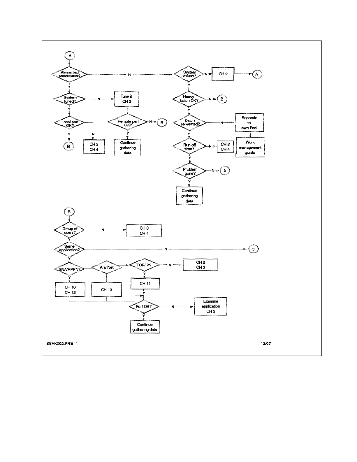
Figure 3. Where to Read, 1 of 2
Chapter 1. Tools Used for Finding Performance Problems 9
Page 24
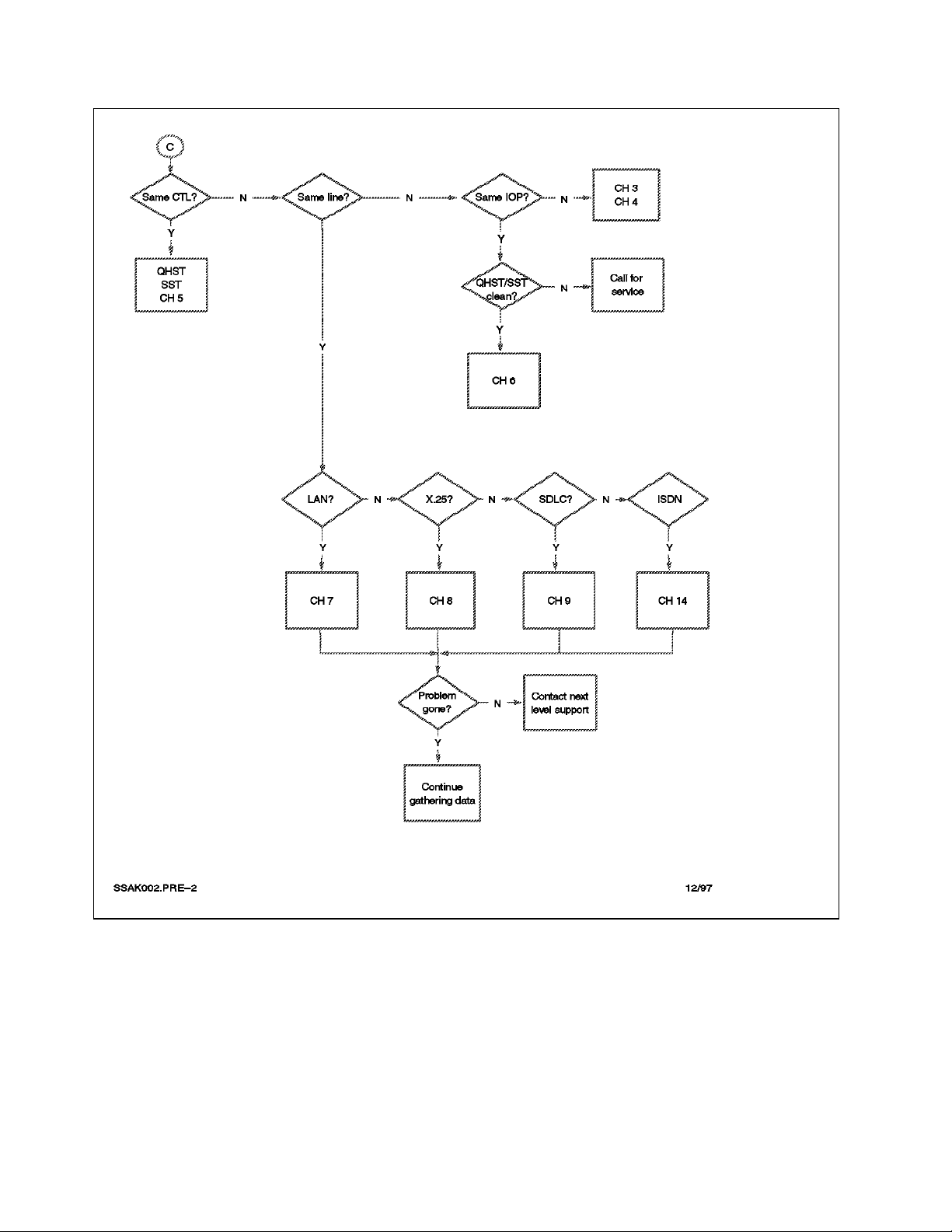
Figure 4. Where to Read, 2 of 2
10 Comm Perf Investigation - V3R6/V3R7
Page 25

Chapter 2. Using CL Commands to Find Performance Problems
This chapter provides information about identifying a communications
performance problem by using command language (CL) commands interactively.
Please bear in mind that using these commands can add a significant amount of
workload to the system, especially if you are using the console display. In other
words, analyzing a performance problem can cause more performance
problems.
2.1 WRKSYSVAL Command
System values are pieces of information that affect the operating environment in
the entire system. System values are not objects and, therefore, they cannot be
passed as parameter values the same as CL variables.
There are some system values that affect performance such as QTOTJOB,
QACTJOB, QMAXACTLVL, QMCHPOOL, and QCMNRCYLMT. Review these
values first because they can relate to your situation.
2.1.1 QTOTJOB
This value controls the total number of jobs for which the storage is allocated
during IPL.
The correct setting of this system value can be obtained by entering the
WRKSYSSTS command. Pay attention to the value displayed in the ″Jobs in
system″ field because the amount of jobs in the system should never be greater
than the value of QTOTJOB. Add 15% to the number of ″Jobs in system″ field
and set this to be the system value QTOTJOB provided that the following
cautions are followed:
•
Remember to clear output queues regularly because OS/400 reserves
storage for a job as long as there is at least one spooled output file for that
job even though the job is inactive. The more files there are in output
queues, the more jobs you see on the Work with System Status display.
•
If you have a high number of spooled files on the system while using the
WRKSYSSTS command and you add 15% more to set the QTOTJOB value,
you significantly increase the time it takes to IPL the system. Performance is
also affected at run time of any system functions that search through the
system wide Work Control Block Table (WCBT). These functions include the
WRKACTJOB command, WRKJOB command, and STRSBS command.
•
Consider using the AS/400 Operational Assistant options to clean the
obsolete spooled files such as old job logs and program dumps from the
system. This can be done by entering
If the amount of ″Jobs in system″ reaches this value, all of the jobs are paged
out from the main storage and the amount of job structures given with the
QADLTOTJ system value (the shipped value is 10) is created before all of the
jobs are paged into the main storage and normal processing continues.
GO CLEANUP on any command line.
You can suspect a wrong setting of QTOTJOB if the system seems to ″slow
down″ periodically with no apparent reason such as a heavy batch job visible.
The ″hang up″ situation normally lasts a couple minutes after which normal
Copyright IBM Corp. 1997 11
Page 26

2.1.2 QACTJOB
processing continues until the previously created job structures are used up and
a new ″hang up″ situation arises.
The value shipped with the operating system is 30 which normally is not large
enough.
Note: A change of this system value is effective only after the next IPL.
This value controls the initial number of active jobs for which storage is to be
allocated during IPL. The amount of storage allocated for each active job is
approximately 110K.
The correct setting for this value can be determined by entering the
WRKACTJOB command; on the right-hand top corner of the display is the
amount of active jobs in the system. Find out what is the highest amount of the
active jobs during a busy day, add 10% to the number, and you have found the
correct setting for the QACTJOB system value. The number of active jobs
should not exceed this value, or all of the jobs are paged out from main storage
until a number of job structures given with QADLACTJ are created.
You can suspect a wrong setting of QACTJOB if the system seems to ″fall
asleep″ periodically with no apparent reason visible. The ″sluggish
performance″ situation normally lasts a couple of minutes after which normal
processing continues until the amount of previously created job structures are
used up and a new ″hang up″ situation arises.
The value shipped with the operating system is 20 which normally is not large
enough.
Note: A change of this system value is effective only after the next IPL.
You must keep QACTJOB, QTOTJOB, QADLACTJ, and QADLTOTJ at
reasonable values. If you make QACTJOB and QTOTJOB excessively high,
the IPL is slower due to excessive storage allocation. If you make QACTJOB
and QTOTJOB too small for your environment and you make QADLTOTJ and
QADLACTJ excessively large, run-time performance can be impacted.
2.1.3 QMAXACTLVL
This value determines the maximum activity level of the system. This is the
number of all the jobs that can compete at the same time for main storage and
processor resources. If a job cannot be processed because no activity levels
are available, the job is held until another job reaches a time slice end or a long
wait. See Chapter 14 in the
state transitions.
Even though the value shipped with V3R7 is *NOMAX, ensure that this is the
setting on your AS/400 system. This is because the value shipped with the
previous releases (prior to V3R1M0) was 100 and normally the system values are
not changed during the update of the operating system. A change to this system
value takes effect immediately.
Do Not Set the Values Too Large!
Work Management Guide
for information about job
12 Comm Perf Investigation - V3R6/V3R7
Page 27

2.1.4 QMCHPOOL
This system value affects the size of the *MACHINE storage pool. The machine
storage pool contains the highly-shared microcode and operating system
programs. Some of the programs are pageable and some of them are not
pageable. This means that you must be careful when changing the size for this
storage pool because system performance may be impaired if the storage pool
is too small.
Notes:
1. A change to this system value takes effect immediately. The shipped value
2. This value may be changed by the performance adjust support when the
You can also change the setting of the QMCHPOOL system value by using the
Work with System Status display as described in the Section 2.4, “WRKSYSSTS
Command” on page 16.
The third way of changing this system value is done by using the WRKSHRPOOL
(Work with Shared Pools) command.
2.1.5 QCMNRCYLMT
This system value provides recovery limits for system communications recovery.
It specifies the number of recovery attempts to make and when to send an
inquiry message to the system operator if the specified number of recovery
attempts has been reached.
is 20000KB.
system value QPFRADJ is set to 1, 2, or 3.
The recommended value is (2 5), which means that two communication line or
control unit retries are tried within a 5-minute interval. Never set the first value
(count limit) equal to or greater than the second value (time interval) excluding
(0 0).
If the count limit is 0, regardless of the time interval, no recovery attempts are
made. When the count limit is greater than 0 and the time interval is 0, infinite
recovery attempts are being made. If the count limit is greater than 0 and the
time interval is greater than 0, the specified number of recovery attempts are
made and an inquiry message is sent to the operator after the specified time
interval.
Table 1. QCMNRCYLMT Settings Examples
Count Limit Time Interval Action
0 0 No recovery
0 1 through 120 No recovery
1 through 99 0 Infinite recovery
1 through 99 1 through 120 Count and time recovery
An incorrect setting of a QCMNRCYLMT value can cause the system to perform
the line or controller recovery continuously. Under some conditions, the
continuous retries can consume a significant amount of system resources. If this
occurs, stop the process by varying the configuration object off.
Chapter 2. Using CL Commands to Find Performance Problems 13
Page 28

2.2 PRTERRLOG Command
The next step of solving a communications performance problem is to verify that
the hardware is functioning properly. This can be done with the PRTERRLOG
(Print Error Log) command that is used primarily for problem analysis tasks. The
command places a formatted printer file of the data in the system error log (in
case there are errors reported) into a spooled printer device file named
QPCSMPRT or into a specified output file.
This command is shipped with public *EXCLUDE authority. The following user
profiles have private authorities to use the command: QPGMR, QSYSOPR,
QSRV, and QSRVBAS.
The first page of the PRTERRLOG command prompt looks similar to the following
display:
Type choices, press Enter.
Type of log data to list . . . . *ALL
Logical device . . . . . . . . . *ALL
+ for more values
Resource name . . . . . . . . . Name
+ for more values
Error log identifier . . . . . . Hexadecimal value
+ for more values
Output . . . . . . . . . . . . . *PRINT *PRINT, *OUTFILE
Time period for log output:
Beginning time . . . . . . . . *AVAIL Time, *AVAIL
Beginning date . . . . . . . . *CURRENT
Ending time . . . . . . . . . *AVAIL
Ending date . . . . . . . . . *CURRENT
Print format . . . . . . . . . . *CHAR
F3=Exit F4=Prompt F5=Refresh F12=Cancel F13=How to use this display
F24=More keys
Print Error Log (PRTERRLOG)
*ALL, *ALLSUM, *ANZLOG...
Name, *ALL
Date, *CURRENT
Time, *AVAIL
Date, *CURRENT
*CHAR, *HEX
More...
Figure 5. PRTERRLOG Command Prompt
You can also view the error log by using the System Service Tool as described
in Chapter 5, “Using System Service Tools” on page 71.
If the list produced with the Print Error Log command contains no hardware
errors in lines, controllers, or IOPs, proceed with the next topic. Otherwise,
contact your hardware service provider.
2.3 PTF Commands
This topic provides only part of the information about working with PTFs. For
more information, see Chapter 4 in
Handling
Install the latest cumulative PTF package about every four months or at least
twice a year. This is to ensure that your system has the latest level of code
14 Comm Perf Investigation - V3R6/V3R7
, SC41-4206.
AS/400 System Startup and Problem
Page 29

installed, and usually most of the so-called ″performance PTFs″ are included in
the cumulative PTF packages.
IBM creates PTFs to correct problems or potential problems found within IBM
licensed programs. PTFs may fix problems that appear to be hardware failures,
or they may provide new or enhanced functions.
2.3.1 DSPPTF
The Display Program Temporary Fix (DSPPTF) command shows the program
temporary fixes (PTFs) for a specified product.
To find out what level of code is running on the system, type the DSPPTF 5716999
command on any command line and you receive the ″Display PTF Status″
display. The first line displayed shows you the latest cumulative PTF package
installed on your system.
2.3.2 SNDPTFORD
To find out what the latest PTF package is, enter the SNDPTFORD
PTFID((SF98370)) command and press Enter. I f you have a maintenance
agreement with IBM, you receive a file that has information about:
•
PTF packages available for Version 3 Release 7
•
Installing the latest cumulative package
•
Preventive service planning (PSP) information for installing the latest
cumulative PTF package
•
PSP information for installing Version 3 Release 7
•
IBM frequently-asked questions about the AS/400 system
•
Summary of the Version 3 Release 7 High Impact/Pervasive (HIPER) PTFs
and PTFs that are in error (PE)
•
Complete detailed list of the Version 3 Release 7 PTFs that are in error (PE)
•
Complete detailed list of the Version 3 Release 7 High Impact/Pervasive
(HIPER) problems
•
Summary of the generally available Version 3 Release 7 PTFs
Enter the SNDPTFORD PTFID((SF97370)) command to obtain a listing that
provides you with a convenient reference of the License Internal Code fixes and
program temporary fixes (PTFs) that are available by IBM licensed program
categories. This listing is updated regularly. You may choose to order a
PTF/FIX that effects one of your IBM licensed programs.
Enter the SNDPTFORD PTFID((SF99370)) command to order the latest cumulative
PTF package that is available in your country.
Information about the latest performance PTFs can also be obtained by reading
item 130NC in HONE.
Chapter 2. Using CL Commands to Find Performance Problems 15
Page 30

2.4 WRKSYSSTS Command
Observe and balance the overall (system wide) performance before focusing on
a communications performance problem. The reason for this is that the
communications performance is only a relatively small part of the overall
performance. If the entire system is functioning poorly, there normally is no use
trying to figure out what might be wrong with communications.
2.4.1 WRKSYSSTS
The Work with System Status display shows the current status of the system in
real time. Use this display to observe the paging fault rates and job transitions.
The indicators you need to pay special attention to (in order of priority) are:
1. Non database fault rates in the machine pool
2. Non database fault rates in all the other pools
3. Page rates in all the pools
4. Transition rates in all the pools
Note: When tuning the system, make sure that the machine pool is treated
separately from the other pools.
Use the faulting guidelines in the
Work Management Guide
manual and
Appendix I, “Guidelines for Interpreting Performance Data” on page 379 to
determine the effects that faulting has on performance. The following examples
may help you to understand the faulting guidelines:
•
The response time of an interactive transaction is affected by any faults that
occur during that transaction. Each fault adds from 10 to 30 milliseconds to
the end-user′s response time. For example, if the disk response time is 20
milliseconds and the transaction has five faults per transaction, add about
0.1 seconds to the total response time.
•
Each fault consumes a certain amount of the CPU power: the more faults that
occur, the more CPU is being consumed for unproductive work. In the
following examples, processing the transactions consumes 70% of the CPU
capability and the faulting rate is 100.
− On a 9401 class (CPW close to 7) processor, these faults use CPU for 0.6
seconds.
− On an 9402 model 2130 class (CPW close to 12) processor, these faults
use CPU for 0.3 seconds.
− On an 9406 530 class (CPW close to 132) processor, these faults use CPU
for 0.02 seconds.
If the faulting rate of your system is close to the poor end of the faulting
guidelines tables, approximately 10% to 20% of the CPU is used for faulting.
Adding main storage to reduce the faulting rate also lowers the CPU
utilization, thus leaving more processing power available to handle more
transactions.
•
With the increasing faulting rate, the amount of disk I/O also increases. If
you have only a few actuators, these faults can cause the disk utilizations to
increase more rapidly than if you have many disk arms. As your disk arm
(actuator) utilization increases, the time to process disk I/Os increases and
the response times get longer.
16 Comm Perf Investigation - V3R6/V3R7
Page 31

While using the Work with System Status display to analyze a communication
performance problem, concentrate on two storage pools:
*MACHINE pool
This is the pool in which the OS/400 jobs and microcode tasks run.
Normally this is the pool that should have the rate of non-DB faults
below 10 faults per second.
OTHER pool
This is the pool in which the communications jobs are routed to. The
shipped value for this is the *BASE pool. Investigate the subsystem
descriptions for QCMN and QSERVER subsystems to see which
storage pool is being used by the jobs and focus on that storage pool.
•
What is the faulting rate in the *MACHINE pool? See Table 17 on page 379
for guidelines of non-database page faults in the storage pool. If the rate is
not acceptable, see the map in Figure 7 on page 20.
•
What is the faulting rate in the storage pool used for communications jobs?
•
A rule of thumb for the initial Activity Level Factor used for the
communications subsystem is 500K per activity level (for example, 4000K of
memory and an activity level of 8 should provide adequate resources for
interactive work). If 500K per activity level is not enough, add memory to the
pool or decrease the activity level in the pool.
Remember to provide enough activity levels in the pool where the
communication jobs are running or you may experience a significant
performance degradation. Please note that file transfer jobs require
considerably more memory than interactive jobs so a rule of thumb for a file
transfer job is a 2000K per transfer.
•
If you have Client Access/400 users running critical file transfer functions,
consider separating the transfer jobs to a storage pool of their own. Create
a new storage pool for subsystem QCMN and direct the routing entry having
the compare value
QTFDWNLD to that pool. The following table describes the
routing entries that you may work with to override the IBM supplied default
values:
Table 2. IBM Supplied Program Routing Entry Compare Values for V3R7
Compare Value Subsystem Description Function
′QCNPCSUP ′ QBASE, QCMN CLIENT ACCESS/400 SHARED FOLDERS 0, 1
′QCNTEDDM ′ QSYSWRK DDM
′QHQTRGT ′ QBASE, QCMN CLIENT ACCESS/400 REMOTE DATA QUEUE
′QLZPSERV ′ QBASE, QCMN CLIENT ACCESS/400 LICENSE MANAGER (ORIGINAL CLIENTS)
′QMFRCVR ′ QBASE, QCMN CLIENT ACCESS/400 MESSAGE SENDER
′QMFSNDR ′ QBASE, QCMN CLIENT ACCESS/400 MESSAGE RECEIVER
′QNPSERVR ′ QBASE, QCMN CLIENT ACCESS/400 NETWORK PRINT SERVER
′QOCEVOKE ′ QBASE, QCMN CROSS-SYSTEM CALENDARING
′QOQSESRV ′ QBASE, Q CMN DIA VERSION 2 (Prestart Job Entry)
′QRQSRV ′ QBASE, QCMN REMOTE SQL - DRDA
′QTFDWNLD ′ QBASE, QCMN CLIENT ACCESS/ 400 FILE TRANSFER FACILITY
′QZDAINIT ′ QSERVER DATABASE SERVERS (ODBC and Remote SQL)
′QZHQTRG ′ QBASE, QCMN CLIENT ACCESS/400 REMOTE DATA QUEUE SERVER
′QZRCSRVR ′ QBASE, QCMN CLIENT ACCESS/400 REMOTE COMMAND SERVER
′QZSCSRVR ′ QBASE, QSRV CLIENT ACCESS/400 CENTRAL SERVER
′QVPPRINT ′ QBASE, QCMN CLIENT ACCESS/ 400 VIRTUAL PRINT
Chapter 2. Using CL Commands to Find Performance Problems 17
Page 32

% CPU used . . . . . . . : 32.3 System ASP . . . . . . . : 11.80 G
Elapsed time . . . . . . :600:22:59 % system ASP used . . . : 77.0307
Jobs in system . . . . . : 5611 Total aux stg . . . . . : 11.80 G
% perm addresses . . . . : .007 Current unprotect used . : 315 M
% temp addresses . . . . : .016 Maximum unprotect . . . : 695 M
Sys Pool Rsrv Max -----DB----- ---Non-DB--- Act- Wait- ActPool Size K Size K Act Fault Pages Fault Pages Wait Inel Inel
1 59488
2 73564 0 19
3 512
4 183352
5 12300
6 64000
===>
F21=Select assistance level
2 33980 +++ .0 .0 11.2 1.4 8.9 .0 .0
Work with System Status SYSNM005
10/25/96 11:48:34
5
.2 .2 .4 1.2 12.3 .1 .0
01 .0 .0 .0 .0 .0 .0 .0
05 .0 .1 .4 5.5 11.4 .0 .0
03 .0 .0 .0 .0 .0 .0 .0
084.0 .0 3.1 .2 1.4 .0 .0
Bottom
Figure 6. The Preferred WRKSYSSTS Display
Notes:
1 This column is the most important column of this display. Because
the machine pool contains objects used system-wide, page faulting in this
pool affects all of the jobs in the system. Therefore, it is desirable to
maintain a low page fault rate in this pool. The only way to affect the
paging in the machine pool is to adjust the size of the pool.
See Table 17 on page 379 for guidelines of non-database page faults in
*MACHINE pool.
the
2 The rule of thumb for adjusting the machine pool size is to multiply
the number in the ″Reserved Size″ field by one and a half.
3 This column represents the sum of non-database faults in all of the
storage pools and this is the column you need to focus your attention on.
The non database faults include program code (jobs′ work areas and
variables, for example). To affect the faulting rate in the pool (except
machine pool), you can change either the size or the activity level of the
pool.
See Table 18 on page 379 and Table 19 on page 380 for guidelines about
the amount of faults in storage pools.
4 This column represents the sum of database faults in all of the
storage pools. Please remember that a system with no database faults is
a ″dead″ system. This is because the data may be changed only when
the data is in the main storage and if the data is not in the main storage,
the system issues a fault. When no database pages are brought into the
main storage, not a single piece of data is being changed and no work is
done with the system.
18 Comm Perf Investigation - V3R6/V3R7
Page 33

Basically, a fault is an order to go and get a piece of data from a disk to
main storage so that the data can be changed. Technically speaking, a
page fault is a program notification that occurs when a page that is
marked as not in main storage is referred to by an active program.
5 These last three columns (from left to right) represent the job′s state
transitions. When the pool size and activity level settings are in balance
with each other, the ratio of columns (from left to right) should be 10 to
one. Usually, when the pool size and activity level settings are correct for
the workload, the transition rates fall within the guidelines.
A job running on the system is in one of the following states:
Active The job is in main storage and it is processing work that is
requested by the application.
Wait The job needs to use a resource that is momentarily
unavailable.
Ineligible The job has all of the resources required to do the
processing, but it is waiting for a free activity level.
Wait-to-ineligible transitions need not be zero all of the time. When there
is a momentary period of heavy usage, it may be better to let the jobs
become ineligible to avoid excessive page fault rates or thrashing.
See Table 20 on page 380 for guidelines of the ratio of
Wait-to-Ineligible/Active-to-Wait transitions.
6 The time frame of the observation period should be kept between five
and 30 minutes. If the observation period is less than five minutes, the
occasional peak loads tend to distract the rates of both faults and pages.
On the other hand, if the time period is over 30 minutes, the important
data may be lost because the counters holding the data may get wrapped.
2.4.2 Information About Activity Level Guidelines
Table 3. Activity Level
Resource Description Where to Look Compare With
Activity Level for *BASE and
QSPL pool
QINTER Activity Level System Report: Storage Pool
System Report: Storage Pool
Utilization, WRKSYSSTS, ADVISOR
Utilization, WRKSYSSTS, ADVISOR
Figures given in Chapter
14 in the
Management Guide
See Table 22 on
page 380.
2.4.3 Information About Transition Guidelines
Work
.
Table 4. W-I and A-W Ratio
Resource Description Where to Look Compare With
W-I/A-W System Report: Storage Pool
Utilization, WRKSYSSTS
Chapter 2. Using CL Commands to Find Performance Problems 19
See Table 20 on
page 380.
Page 34

2.4.4 Interactive Tuning Roadmap
Balancing your main memory and CPU utilization is accomplished by allocating
the memory available and setting the activity levels in the storage pools. Refer
to the
Work Management Guide
activity level settings.
Note: You have to repeat Step 4 through Step 7 for all of the other pools in your
AS/400 system; Step 3 is for the *MACHINE pool only. F ollow the road map
during periods of high system′s activity because there is no use tuning the
system when there is only a relatively light workload on the system. Make sure
that system value QPFRADJ is set to zero before following the tuning road map.
for the guidelines of both the memory and
Interactive AS/400 Tuning Roadmap
1. Enter command WRKSYSSTS.
Press PF21 to set assistance level to Intermediate.
2. Wait 2-3 minutes and press PF5 to refresh.
3. Does *MACHINE NDB faults meet the guidelines?
a. Yes ... Press PF10 and go to step 4.
b. No .... Adjust QMCHPOOL:
1) -50K if fault rate = 0
2) +50K if fault rate > 3.0
3) Press PF10 to reset and go to step 2.
4. Is the DB fault + NDB fault > 20 in any pool?
a. Yes ... Increase pool size by 50KB, press PF10 and repeat
Step 4 (repeat until all pools are less than 20).
b. No .... Go to step 5.
5. Wait 2-5 minutes, press PF5. Press PF21 to set the Assistance
level to Advanced.
Is the Wait to Ineligible state = 0?
a. Yes ... Reduce Activity level by 2, press PF10 to reset, and
repeat step 5.
b. No .... Go to step 6.
6. Is the Active to Wait state 10x the activity level?
a. No ....System not heavily used or complex application mix,
b. Yes ... Go to step 7.
7. Is the sum of all fault rates for all pools within guidelines?
a. No .... Go to step 4.
b. Yes ... Go to step 8.
8. Activity levels and pool sizes probably OK. Continue monitoring
Figure 7. AS/400 Tuning Roadmap
WRKSYSSTS display regularly.
20 Comm Perf Investigation - V3R6/V3R7
go to step 4.
Page 35

2.5 WRKACTJOB Command
The Work with Active Jobs command measures system performance by
measuring aspects such as the CPU usage and response time. The following
examples show the different Work with Active Jobs displays.
To view the Work with Active Jobs display, type
and press the Enter key. Press the PF21 key to show more jobs on one display
as in the following example:
CPU %: 3.4 Elapsed time: 00:22:42 Active jobs: 119
Opt Subsystem/Job User Type CPU % Function Status
QBATCH QSYS SBS .0 DEQW
QCMN QSYS SBS .0 DEQW
USERPC COOK EVK .0 * -PASSTHRU EVTW
USERPC COOK EVK .0 * -PASSTHRU EVTW
P23ARTYC AS0219R EVK .0 * -PASSTHRU EVTW
P23ARTYC AS0219R EVK .0 * -PASSTHRU EVTW
QCTL QSYS SBS .0 DEQW
QJSCCPY A960303A BCH .0 PGM-QSCCPY DEQW
QSYSSCD QPGMR BCH .0 PGM-QEZSCNEP EVTW
QINTER QSYS SBS .0 DEQW
USERPCF USER INT .0 CMD-STRSST DEQW
USERPCI USER INT .2 CMD-DSPLOG DSPW
QPADEV0006 A960303A INT .0 CMD-WRKSYSSTS RUN
QPADEV0016 A960303B INT .0 CMD-DSPMSG DSPW
QPADEV0017 A960303B INT .0 MNU-MAIN DSPW
QPADEV0021 A960303C INT .2 CMD-WRKQRY DSPW
===>
F21=Display instructions/keys
Work with Active Jobs SYSNM005
WRKACTJOB on any command line
10/25/96 11:48:49
More...
Figure 8. WRKACTJOB after Pressing PF21
More information is displayed after pressing the PF11 (Display elapsed data) key:
Chapter 2. Using CL Commands to Find Performance Problems 21
Page 36

CPU %: 3.4 Elapsed time: 00:22:42 Active jobs: 119
Opt Subsystem/Job Type Pool Pty CPU Int Rsp AuxIO CPU %
QBATCH SBS 2 0 .6 3 .0
QCMN SBS 2 0 2.9 1 .0
USERPC EVK 2 20 .0 0 .0
USERPC EVK 2 20 .0 0 .0
P23ARTYC EVK 2 20 .1 0 .0
P23ARTYC EVK 2 20 .0 0 .0
QCTL SBS 2 0 1.0 6 .0
QJSCCPY BCH 2 10 .1 78 .0
QSYSSCD BCH 2 10 .3 0 .0
QINTER SBS 2 0 2.8 0 .0
USERPCF INT 4 20 2.7 0 .0 0 .0
USERPCI INT 4 20 14.7 140 .2 428 .2
QPADEV0006 INT 4 20 15.6 19 .1 218 .0
QPADEV0016 INT 4 20 21.0 0 .0 0 .0
QPADEV0017 INT 4 20 .4 0 .0 0 .0
QPADEV0021 INT 4 20 17.8 160 .0 524 .2
===>
F21=Display instructions/keys
Work with Active Jobs SYSNM005
10/25/96 11:48:49
More...
Figure 9. WRKACTJOB after Pressing PF11
You may place the cursor on any column and arrange the display in a
descending sequence, for example:
•
CPU %
•
Response time
•
DISK I/O
CPU %: 3.4 Elapsed time: 00:22:56 Active jobs: 119
Opt Subsystem/Job Type Pool Pty CPU Int Rsp AuxIO CPU %
USERPCI INT 4 20 14.7 142 .2 431 .2
QPADEV0006 INT 4 20 15.8 21 .1 228 .0
QPADEV0021 INT 4 20 17.9 161 .0 524 .2
QPADEV0017 INT 4 20 .4 0 .0 0 .0
QPADEV0016 INT 4 20 21.0 0 .0 0 .0
USERPCF INT 4 20 2.7 0 .0 0 .0
X2507 BCH 2 40 2.5 25 .0
X2506 BCH 2 40 .0 0 .0
TCPIPLOC BCH 2 40 .0 0 .0
TARGET2 BCH 2 40 .0 0 .0
TARGET1 BCH 2 40 .0 0 .0
SCPF SYS 2 40 38.9 24 .0
SYSTEM49 BCH 2 40 .1 0 .0
SYSTEM40 BCH 2 40 .0 0 .0
ARHIPPA3 BCH 2 40 .0 0 .0
SYSTEM12 BCH 2 40 .0 0 .0
===>
F21=Display instructions/keys
Work with Active Jobs SYSNAM05
10/25/96 11:49:03
More...
Figure 10. WRKACTJOB Sequenced by Response Time
22 Comm Perf Investigation - V3R6/V3R7
Page 37

Pay attention to the following subjects:
•
Is a communications job consuming a relatively great deal of CPU?
•
Are there any communications jobs creating lots of I/O?
− If there is, display the job by entering a number five in front of the job
− Are there many files opened?
− Are there many logical files opened?
− Can a similar task be done on a locally attached terminal?
− Is the response time the same in both cases?
− If it is, go and see what the application is doing.
− Can the application itself be modified?
2.6 Using WRKDSKSTS
The Work with Disk Status display shows performance and status information
about the disk units on the system. Type the WRKDSKSTS command on the
command line and press the Enter key. The Work with Disk Status display is
shown:
and you receive the ″Work with Job″ display.
Elapsed time: 00:00:00
Size % I/O Request Read Write Read Write %
Unit Type (M) Used Rqs Size (K) Rqs Rqs (K) (K) Busy
1 6606 1967 82.0 .0 .0 .0 .0 .0 .0 0
1 6606 1967 82.0 .0 .0 .0 .0 .0 .0 0
3 6606 1475 75.9 .0 .0 .0 .0 .0 .0 0
4 6606 1475 76.0 .0 .0 .0 .0 .0 .0 0
5 6606 1967 76.0 .0 .0 .0 .0 .0 .0 0
6 6606 1967 76.0 .0 .0 .0 .0 .0 .0 0
7 6606 1475 75.9 .0 .0 .0 .0 .0 .0 0
8 6606 1475 76.0 .0 .0 .0 .0 .0 .0 0
Command
===>
F3=Exit F5=Refresh F12=Cancel F24=More keys
Work with Disk Status SYSNM005
10/25/96 11:49:17
Bottom
Figure 11. The WRKDSKSTS Display
Note: Before observing disk status, have your system tuned according to either
Figure 7 on page 20 or as described in Chapter 14 in the
.
Guide
When viewing the Work with Disk Status display, pay attention to the percent
busy data that is actually the estimated percentage of time the disk unit is being
used during the elapsed time. This estimate is based on:
Chapter 2. Using CL Commands to Find Performance Problems 23
Work Management
Page 38

•
The number of I/O requests
•
The amount of data transferred
•
The performance characteristics of the type of disk unit
Each unit (actuator) should be less than 50% busy. An actuator is the device
within an auxiliary storage device that moves the read and write heads. If each
unit is between 50% and 70% busy, you may experience variable response
times. In case all the units are more than 70% busy, the amount of actuators is
inadequate for the workload in the system. If you have a well-tuned system with
actuators exceeding the 50% busy guideline, increase the number of disk
actuators.
It is possible to experience unacceptable performance even if only one actuator
exceeds the 50% busy guideline. This usually happens when frequently-used
data is placed on a single actuator. If this happens on your system, use the
Performance Tools/400 licensed program to run the disk report to find out which
data is frequently used. After identifying the data causing the bottleneck, you
can save the data, delete the data, and restore the data to spread it across all of
the actuators.
A batch job accessing the data can cause a short time period of an actuator
exceeding the 50% guideline. If the data is not concentrated on a single
actuator, you notice the high percentage of the utilization moving from one unit
to another unit.
Note: Please remember that observation periods of less than five minutes
usually do not provide reliable results.
To notice either improving or degrading trends in the disk performance, observe
the historical data created from the regularly collected performance data.
2.7 WRKSYSACT Command
This command is a part of the Performance Tools/400 licensed program and is
actually an enhancement of the Work with Active Jobs display. It is the only tool
that shows both external jobs and internal tasks at the same time on the display.
By default, the jobs are sequenced by CPU usage but you can also sequence the
display by I/O.
•
Are there any communications related modules consuming CPU?
•
Are there any communications related modules consuming Disk?
− If the answer is yes, contact your service provider to find out if there are
any Program Temporary Fixes available for these modules.
Notice!
The performance statistics reported by this function represent activity that
has occurred since a previous collection. This implementation may be
different from other system functions that generally provide cumulative
values until specifically reset.
If the Performance Tools/400 licensed program is installed on your system, enter
the WRKSYSACT command on any command line to receive the following
display:
24 Comm Perf Investigation - V3R6/V3R7
Page 39

Automatic refresh in seconds . . . . . . . . . . . . . . . . . 5
Elapsed time . . . . : 00:00:03 Overall CPU util . . : 2.6
Type options, press Enter.
1=Monitor job 5=Work with job 1234
Job or CPU Sync Async PAG
Opt Task User Number Pty Util I/O I/O Fault
5QPADEV0006 A960303A 060789 1 .9000
QPADEV0021 A960303C 060812 20 .5 0 0 0
QTGTELNETS QTCP 060229 20 .4 2 0 1
QJSCCPY A960303A 060839 10 .1 0 1 0
VTMTS1 0 .1 0 0 0
IPR2050103 0 .1 0 0 0
SMPO0006 0 .1 15 0 0
CFINT1 0 .1 0 0 0
F3=Exit F10=Update list6F11=View 2 F12=Cancel F19=Automatic refresh
F24=More keys7
Work with System Activity
Total Total
Bottom
Figure 12. WRKSYSACT Display View 1 is a Summary Display
Notes:
1 This column displays the run priority of the job.
2 This column displays the CPU utilization of the job.
3 This column displays the total amount of synchronous I/O the job is
causing. Having a low amount of synchronous I/O is important because a
job has to wait for the completion of the synchronous I/O operation before
continuing.
4 This column displays the total amount of asynchronous I/O caused by
the job. The amount of asynchronous I/O is of less importance than the
amount of synchronous I/O because a job can continue processing
immediately after requesting an asynchronous I/O. In a way, an
asynchronous I/O is similar to a batch job; after having submitted it, you
do not have to wait for its completion.
5 By entering ″1″ in this field, you can monitor this job only and by
entering ″5″, you access the ″Work With Job″ display. You can monitor up
to 20 jobs and tasks at a single time.
6 By pressing the PF11 key, you can select from three different
displays: the summary, Synchronous I/O details, and Asynchronous I/O
details.
7 Press the PF24 key for additional function keys to use. Press the
PF14 key to display jobs only and exclude the information for tasks. Press
the PF15 key to display tasks only and exclude the information for jobs.
You can also use the PF16 key to display the jobs/tasks in a descending
order of disk I/O operations.
Chapter 2. Using CL Commands to Find Performance Problems 25
Page 40

Automatic refresh in seconds . . . . . . . . . . . . . . . . . 5
Elapsed time . . . . : 00:00:03 Overall CPU util . . : 2.6
Type options, press Enter.
1=Monitor job 5=Work with job
Job or CPU DB DB Non-DB Non-DB
Opt Task User Number Pty Util Read Write Read Write
QPADEV0006 A960303A 060789 1 .9 0 0 0 0
QPADEV0021 A960303C 060812 20 .5 0 0 0 0
QTGTELNETS QTCP 060229 20 .4 0 0 2 0
QJSCCPY A960303A 060839 10 .1 0 0 0 0
VTMTS1 0 .1 0 0 0 0
IPR2050103 0 .1 0 0 0 0
SMPO0006 0 .1 0 0 0 15
CFINT1 0 .1 0 0 0 0
F3=Exit F10=Update list F11=View 3 F12=Cancel F19=Automatic refresh
F24=More keys
Work with System Activity
--------Synchronous---------
Bottom
Figure 13. WRKSYSACT Display View 2, Details of Synchronous I/O
Automatic refresh in seconds . . . . . . . . . . . . . . . . . 5
Elapsed time . . . . : 00:00:03 Overall CPU util . . : 2.6
Type options, press Enter.
1=Monitor job 5=Work with job
Job or CPU DB DB Non-DB Non-DB
Opt Task User Number Pty Util Read Write Read Write
QPADEV0006 A960303A 060789 1 .9 0 0 0 0
QPADEV0021 A960303C 060812 20 .5 0 0 0 0
QTGTELNETS QTCP 060229 20 .4 0 0 0 0
QJSCCPY A960303A 060839 10 .1 0 1 0 0
VTMTS1 0 .1 0 0 0 0
IPR2050103 0 .1 0 0 0 0
SMPO0006 0 .1 0 0 0 0
CFINT1 0 .1 0 0 0 0
F3=Exit F10=Update list F11=View 1 F12=Cancel F19=Automatic refresh
F24=More keys
Work with System Activity
--------Asynchronous--------
Bottom
Figure 14. WRKSYSACT Display View 3, Details of Asynchronous I/O
26 Comm Perf Investigation - V3R6/V3R7
Page 41

Chapter 3. Using Performance Tools/400
Performance analysis is a method of investigating, measuring, and correcting
deficiencies so that system performance meets the user′s expectations. The
problem solving cycle should be similar to:
1. Understand the symptoms of the problem.
2. Use tools to measure and define the problem.
3. Isolate the cause.
4. Correct the problem.
5. Use tools to verify the correction.
Once the apparent cause (or causes) is isolated, you can propose a solution.
The solution can be something simple such as tuning the storage pools, or a
complex one that requires application recoding.
To achieve the optimum performance, you must understand the relationships
between critical system resources and attempt to balance the use of the
resources that are the CPU, the main storage, the disk units, and the
communication lines. However, any improvement can only come through
analyzing the critical resources and contention for both system and application
objects.
3.1 System-Wide Problem Analysis
The ways to analyze the system-wide performance are:
•
Using the CL commands as described in Chapter 2, “Using CL Commands to
Find Performance Problems” on page 11.
•
Using the Performance Tools/400 reports and displays as described in this
chapter.
3.1.1 Advisor
The Advisor provides the easiest way of evaluating the performance data. It is a
tool located between automatic system tuning and performance reports. You
can either enter the Analyze Performance Data (ANZPFRDTA) command or
choose option 10 on the PERFORM menu to start the advisor.
The Advisor uses data collected by the Performance Monitor to recommend
performance tuning changes, and it can also point out other problems affecting
system performance. You can use the Advisor to analyze the performance data
collected from other systems.
The Advisor analyzes one member set of performance data at a time. Select the
member that was collected when the performance problem occurred.
It is easy to find the right time interval to analyze by using the display histogram
function. For example, if you need a time interval when the transactions had the
longest response times, select the transaction response time option on the
Display Histogram display. From the chart, select a time interval by moving the
cursor to that interval, type 1, and press the Enter key. The Advisor analyzes the
Copyright IBM Corp. 1997 27
Page 42

performance data collected during that particular interval and gives you
recommendations and conclusions.
The Advisor analyzes performance data, including:
•
Storage pool sizes
•
Activity levels
•
Disk and CPU utilization percentages
•
Communications line utilization percentages and error rates
•
IOP utilization percentages
•
Unusual job activities such as exceptions or excessive use of system
resources
•
Interactive trace data (when collected)
Note!
To avoid causing a serious performance impact while running the Advisor
interactively, start the advisor by entering the ANZPFRDTA command. Press
the PF4 (prompt) key followed by the PF10 (additional parameters) key to
change the value of the DATATYPE parameter from
*ALL to *SAMPLE. If you
need to analyze the trace data with Advisor, consider submitting the job or
running it when your system has a light workload.
You can either select all of the intervals or a subset of the time intervals for
analysis. You can run the Advisor either interactively or as a batch job. The
output of using the Advisor is grouped under the following headings:
•
Recommendations
•
Conclusions
•
Interval conclusions
All of the headings have information about:
•
CPU utilization of high priority (with a run priority 20 or higher) jobs
•
Performance analysis of interactive transactions by using the trace data
collected with the performance monitor
•
Main storage utilization and Wait-To-Ineligible versus Active-To-Wait ratio.
This addresses page faulting and activity-level analysis.
•
Disk utilization and other disk activities
•
IOP utilization
•
System impact of authority lookups
•
System impact of exceptions
•
Communication line utilization and error percentages
The Advisor does not:
•
Make any recommendations for modifying specific programs to improve their
performance.
•
Analyze noninteractive trace data.
The recommendations may include changes to the system′s basic tuning values
that can improve performance. They also may list problems that (when solved)
can solve other performance problems.
28 Comm Perf Investigation - V3R6/V3R7
Page 43

The conclusions display lists conditions that may have affected performance
during the data collection. Good examples of conclusions are:
•
Thresholds reached
•
Save and restore activities
•
Communications line errors
You can use the conclusions that are not related to recommendations as guides
for collecting more performance data or for adjusting the system.
The Advisor may suggest changes to pool sizes and activity levels. These
changes are not made dynamically but only after the operator tells the advisor to
make the changes or to ignore the recommendations. The tuning is done by
pressing the PF9 key on the display recommendations display. Pool and activity
level changes can be made to all of the main storage pools on the system.
The Advisor also suggests which report to run to get more information for your
problem analysis. See the ″Advisor″ chapter of the
SC41-4340, for detailed information.
3.1.2 Performance Graphics
Performance data collected by the performance monitor can also be displayed in
a graphical format. The graphs can either be displayed interactively, or printed
or plotted to hardcopy. The printing option of the graphs is recommended
because the graphics on the paper are more descriptive. The best printouts are
created by using an *IPDS printer. If you must use a conventional printer, please
check the PAGESIZE parameter of the printer file QPPGGPH in the QPFR library.
Performance Tools Guide
,
You can enter the DSPPFRGPH command or the DSPHSTGPH command, or you
may choose option 9 (
Performance graphics) on the PERFORM menu. You have two
types of performance graphics to choose from:
•
Option 1. Display performance data graphics:
Performance data graphs are graphs that:
− Use select/omit criteria.
− Are run against the original performance data.
− Are used to show the performance during one data collection only.
•
Option 2. Display historical data graphics:
Historical data graphs are graphs that:
− Use performance data from several collections.
− Are useful when tracking performance trends.
The Display Historical Graph (DSPHSTGPH) command produces a graph from
the historical data created by the Create Historical Data (CRTHSTDTA)
command. The DSPHSTGPH command is intended to give you a historical
perspective of the system performance in a graphical presentation.
You must run the Create Historical Data (CRTHSTDTA) command for each
member that you want to include in the graph. If no historical data has been
created for a member, it is not included in the graph unless you specify
*YES on
the CRTHSTDTA parameter of the DSPHSTGPH command. You can use the
IBM-supplied format (in the QPFRDATA library) or you can create a format of
your own.
Chapter 3. Using Performance Tools/400 29
Page 44

3.1.3 Print Activity Report
The print activity report (PRTACTRPT) command creates a report using the
performance data collected by the WRKSYSACT command.
You may produce two different reports:
Summary report
Detailed report
The following example shows a summary report:
This prints out a report showing the top 10 list of:
•
CPU intensive jobs and tasks
•
I/O intensive jobs and tasks
This prints out either:
•
Selected numbers of entries for each interval specified by the
PERIOD parameter.
•
The number of entries specified by the NBRJOBS parameter that
are listed in the order specified by the SEQ parameter.
System Activity Report 10/22/96 12:45:18
Member . . . . : QAITMON Report Type . . . . : SUMMARY Version . . . . : 3 Started . . . . : 10/22/96 12:42:50
Library . . . . : QPFRDATA Release . . . . : 6.0 Stopped . . . . : 10/22/96 12:44:31
Order by CPU Utilization:
Job or CPU Sync Async PAG DB DB Non-DB Non-DB DB DB Non-DB Non-DB
Task User Number Pty Util I/O I/O Fault Read Write Read Write Read Write Read Write
---------- ---------- ------ --- ---- ----- ----- ----- ----- ----- ------ ------ ----- ----- ------ -----QPADEV0002 A960303A 059734 20 2.1 574 364 232 0 0 571 3 0 0 358 6
SMAI0004 0 1.6 1 0 0 0 0 0 1 0 0 0 0
SMAI0007 0 1.5 0 0 0 0 0 0 0 0 0 0 0
WRKSYSACT A960303A 059747 1 .5 00000000000
IOSTATSTAS K 0 .3 0 0 0 0 0 0 0 0 0 0 0
CFINT1 0 .3 0 0 0 0 0 0 0 0 0 0 0
QBRMNET QPGMR 059270 30 .2 0 0 0 0 0 0 0 0 0 0 0
QTGTELNETS QTCP 059276 20 .1 0 0 0 0 0 0 0 0 0 0 0
IOP6512010 003 0 .1 0 0 0 0 0 0 0 0 0 0 0
SMXCSPRVSR 0 .0 0 0 0 0 0 0 0 0 0 0 0
Order by Total I/O:
Job or CPU Sync Async PAG DB DB Non-DB Non-DB DB DB Non-DB Non-DB
Task User Number Pty Util I/O I/O Fault Read Write Read Write Read Write Read Write
---------- ---------- ------ --- ---- ----- ----- ----- ----- ----- ------ ------ ----- ----- ------ -----QPADEV0002 A960303A 059734 20 2.1 574 364 232 0 0 571 3 0 0 358 6
QTGTELNETS QTCP 059276 20 .1 0 0 0 0 0 0 0 0 0 0 0
WRKSYSACT A960303A 059747 1 .5 00000000000
SMAI0007 0 1.5 0 0 0 0 0 0 0 0 0 0 0
SMAI0004 0 1.6 1 0 0 0 0 0 1 0 0 0 0
QBRMNET QPGMR 059270 30 .2 0 0 0 0 0 0 0 0 0 0 0
IOSTATSTAS K 0 .3 0 0 0 0 0 0 0 0 0 0 0
IPR0050103 --2619 0 .0 0 0 0 0 0 0 0 0 0 0 0
IOP9162010 001 0 .0 0 0 0 0 0 0 0 0 0 0 0
VTMTS1 0 .0 0 0 0 0 0 0 0 0 0 0 0
Job or Task -- Job or task name
User -- User profile associated with the job
Number -- Job number
Pty -- Job or task priority
CPU Util -- Percent of CPU used by the job or task
Total Sync I/O -- Total number of synchronous I/O operations
Total Async I/O -- Total number of asynchronous I/O operations
PAG Fault -- Number of faults involving the process access group
Synchronous I/O --
DB Read -- Number of synchronous database reads
DB Write -- Number of synchronous database writes
Non-DB Read -- Number of synchronous non-database reads
Non-DB Write -- Number of synchronous non-database writes
Asynchronous I/O --
DB Read -- Number of asynchronous database reads
DB Write -- Number of asynchronous database writes
Non-DB Read -- Number of asynchronous non-database reads
Non-DB Write -- Number of asynchronous non-database writes
Total Total -------Synchronous I/O----- ------Asynchronous I/O------
Total Total -------Synchronous I/O----- ------Asynchronous I/O------
Page 1
Figure 15. An Example of PRTACTRPT Output
30 Comm Perf Investigation - V3R6/V3R7
Page 45

Notes:
The upper part of the list shows the jobs sequenced by the CPU
utilization.
The lower part of the list shows the jobs sequenced by the disk I/O.
3.1.4 Performance Tools Reports
Printing performance reports extracts information from previously collected
performance data. You can review the performance of specific jobs or
transactions, or other performance elements. This can be done by choosing
option 3 (print performance report) on the
print performance report display. You may also issue any of the following
commands:
PRTSYSRPT Print System Report
PRTCPTRPT Print Component Report
PRTTNSRPT Print Transaction Report
PRTLCKRPT Print Lock Report
PRTJOBRPT Print Job Interval Report
PRTPOLRPT Print Pool Report
PRTRSCRPT Print Resource Report
PERFORM menu. This leads you to the
PRTTRCRPT Print Batch Job Trace Report
Each of these commands provides you with a different level of information. The
following reports are produced from the sample data collected with the
performance monitor:
•
System report
•
Component report
•
Job report
•
Pool report
•
Resource report
If you collected trace data with the performance monitor, you can produce:
•
Transaction report that can further be extended to:
− Transaction detail report
− Transition detail report
•
Lock report
•
Batch job trace report
In the early stages of problem determination, print only the first two reports
(system report and component report). These help you to determine whether
you need to analyze the problem in more detail or not.
The system report and the component report provide information to evaluate
your system-wide performance. Pay attention to the following items:
•
Average response time in the system report workload
•
Number of transactions for total run time and per hour
•
CPU percent for all levels of priority and also cumulative. The cumulative
value up to and including priority 20 should not exceed 60 per cents provided
no queries are run interactively.
•
Number of database/non-database page faults in each storage pool
Chapter 3. Using Performance Tools/400 31
Page 46

•
Disk (percentage used and utilization of the actuators)
•
Communication lines traffic and IOP utilization
3.1.4.1 System Report
In the system report, you find the basic set of information to compare against
your predefined performance objectives and the guideline tables as shown in
Work Management Guide
•
The system overview workload and resource utilization part shows you what
the system workload is and what is the cost of processing the workload. The
CPU utilization shows the percentage of processing unit time used by each
job type. According to the guidelines, the total CPU utilization should not
continuously exceed 81% (for four-way processors). See Table 16 on
page 379 for other CPU categories.
•
Check the percent of space in use and the utilization of disk on the utilization
part of report; compare those values to Table 16 on page 379. Column ″ops
per second″ and number of disk IOPs installed on the system show whether
or not you are overdriving the IOPs. On a normal distribution of disk
operations, each IOP′s average should be between 30 to 60 per second.
•
Avg util and max util column on the communication part gives you the
average and maximum percentage of the line capacity used during the
measured interval. Compare those values to Table 16 on page 379.
If you find any discrepancies between the system performance report and the
guidelines, go to the component report to find out whether you need to do a
problem analysis on the system performance.
manual.
3.1.4.2 Component Report
The component report provides information about the same components as the
system report but at a greater level of detail.
•
Component interval activity shows the use of CPU, disk, and pools at
selected time intervals. For example:
− Is the transaction rate high in all the intervals?
− Is the same disk unit suffering from high utilization during all of the
intervals?
− Which of the memory pools has the highest faulting rate?
•
Job workload activity shows the activities of each job. You need to perform
problem analysis on a particular job if you find that a job used most of the
disk I/O operation (under column disk I/O) or CPU utilization (CPU util).
•
In the pools storage activity part, you need to look at the columns DB faults
and Non-DB faults. Compare those values to Table 18 on page 379 and
Table 19 on page 380. W ait-to-ineligible need not be zero all of the time, but
it must be less than .25 for good performance. See Table 20 on page 380 for
the guidelines of activity level changes.
•
Disk activity shows average disk activity per hour and the capacity of each
disk. Batch processing may cause a high utilization of individual disk drives.
Batch sequential processing can stay on one drive for some time.
Interactive performance is not normally degraded if the batch jobs are
running in a storage pool of their own. However, if there are many
interactive jobs, a high disk utilization can indicate a performance problem.
32 Comm Perf Investigation - V3R6/V3R7
Page 47

•
The database journal summary includes user journal and system journaling
of access paths disk write counts. No guidelines are provided so you must
record this information over time to determine any increase in the disk I/O
as a result of journaling.
If you need more data on your current system performance before you decide to
analyze, issue the WRKSYSACT command. Refer to Chapter 2, “Using CL
Commands to Find Performance Problems” on page 11 for more information
about that command.
Based on this information, you can decide if there is a problem with the overall
performance of the system.
3.1.5 Memory Performance Displays and Reports
You cannot measure the amount of memory currently in use; you only can
observe the amount of faults that indirectly tell you whether there is enough
main storage or not. The tools used for finding out the memory performance
are:
•
The WRKSYSSTS command
The Work with System Status display shows you in real time what the
demand for main storage is. See Chapter 2, “Using CL Commands to Find
Performance Problems” on page 11 for information about using this
command.
•
The DSPPFRDTA command
The Display Performance Data command provides an interactive interface to
the previously collected data given in the system, component, and interval
reports.
•
DSPACCGRP command and ANZACCGRP command
These commands show for a job or a group of jobs:
− The temporary storage used
− Open files
− File I/O counts
− Active programs
The Display command and Analyze Access Group command provide data on
the size of the ″currently in use″ part of the PAG. The PAG size can be
affected by reducing the number of active programs, the number of display
and database files open, and the number of display formats and database
buffers allocated for the files. See Section 3.4.2.1, “DSPACCGRP and
ANZACCGRP” on page 51 for more information about displaying and
analyzing the access groups.
3.1.5.1 Where to Find Information About Memory Usage
Table 5 (Page 1 of 2). Memory Utilization Information
Resource Description Where to Look Compare With
Machine pool NDB page fault System Report: Storage Pool
Utilization, WRKSYSSTS, Advisor
Sum of DB and NDB page faults
for each pool
System Report: Storage Pool
Utilization, WRKSYSSTS, Advisor
Table 17 on page 379
Table 18 on page 379
Chapter 3. Using Performance Tools/400 33
Page 48

Table 5 (Page 2 of 2). Memory Utilization Information
Resource Description Where to Look Compare With
Sum of DB and NDB page faults in
all pools
Pool size By interval Pool Report: Pool Activity
The pool with the highest fault
rate for each time interval
System Report: Storage Pool
Utilization, WRKSYSSTS, Advisor
Component Report: Component
Interval Activity
Table 19 on page 380
3.1.6 CPU Performance Reports and Displays
•
System report
•
Component report
•
Transaction report
If the interactive utilization percentage of CPU is always more than 85, try
modeling to see if a faster CPU can help.
•
The WRKACTJOB command:
This command allows you to determine:
− What is the utilization percentage of CPU?
− How much does each job use CPU, both in terms of percentage and for
how long a time total?
•
The WRKSYSACT command
3.1.7 A Brief Discussion About Program Exceptions Consuming CPU
Pre-V3R6 systems report a number of exceptions types by the performance tools
Component Report and the Advisor. The reports showed the number of
exceptions per second per interval that occurred; the Advisor shows the percent
of the CPU used by exceptions in an interval. In addition, there are a set of
charts that show the percent of the CPU used as a result of ″n″ number of
exceptions by type per second.
From V3R6, some of the exceptions have been eliminated for one reason or
another, and some of the exception CPU overhead has changed as a result of
the machine implementation or the type of program in which they occur.
3.1.7.1 Program Exceptions
EAO These are gone from V3R6 as a result of the difference in PowerPC
hardware addressing structure. Any data field or report that had
them has been changed to indicate their absence. See Section
3.1.7.3, “Removal of Effective Address Overflow (EAO) Exceptions in
V3R6” on page 36 for more details on why we used to have EAO
exceptions and why now when we use PowerPC technology and 64-bit
addressing, they no longer occur.
Size These are the result of an arithmetic operation in which the receiving
field is too small for the result. They are an application programming
problem and still occur.
The programs should be reviewed and changed to ensure that the
proper receiver field specification is used or that the programming
algorithm is doing the function in a manner to avoid size exceptions.
Using Performance Monitor trace data and Transaction Report
34 Comm Perf Investigation - V3R6/V3R7
Page 49

(PRTTNSRPT RPTTYPE *TRSIT) may provide additional information
about which programs are getting size exceptions.
Verify Verify exceptions occur when trying to resolve an as yet unresolved
pointer.
This exception can occur on the RISC machine and is an application
programming problem. The program should be changed to ensure
that the variable used in a CALL instruction does not change from
one use to the next. Use PEX STATS and PEX TRACE to find out
where it is occurring.
Authority These can occur on the RISC machine and are the result of a system
security setup mismatch.
The same rules apply to fixing these as on pre-V3R6 systems. Us e
authorization lists instead of group profiles and ensure that objects do
not have private authorities on them that are less than the PUBLIC
authority. For example, PUBAUT(*CHANGE) and QPGMR(*USE)
causes authority checking to be done.
Decimal Data This can occur on PowerPC AS/400 systems. It is usually related
to incorrect data specification in application data migrated from other
systems, especially the System/36.
3.1.7.2 CPU Cost Variations
What has changed is the CPU cost for each exception. For the program
exceptions that were tested (Authority, Size, Verify) that can occur on the RISC
machine, the CPU costs varied depending on the type of program model used
when the program was built.
There are three different options that affect the cost:
1. OPM (Original Program Model)
2. ILE with DFTACTGRP(*YES) where the activation group is not already created
3. ILE with DFTACTGRP(*NO)
The results of testing the different exceptions and program models showed
inconsistent variations in the CPU/exception cost. For that reason, there are
multiple costs shown in this document for each type of exception.
The challenge is to know what types of programs are generating the exceptions
on the machine. The exception reporting mechanism does not discriminate
between the types of programs so, in some cases, you have to make an
intelligent guess about the possible severity of the problem.
The test results in Appendix I, “Guidelines for Interpreting Performance Data” on
page 379 were generated by running each type of program on an AS/400 model
500-2142. There were two programs for each case, one that did not get the
exception and one that did. The results were calculated by computing the
difference between the two test cases, calculating the CPU time used per
exception, and extrapolating the results to other PowerPC models using the ratio
of the relative performance ratings between the measured system model and the
other models.
Chapter 3. Using Performance Tools/400 35
Page 50

3.1.7.3 Removal of Effective Address Overflow (EAO) Exceptions in
V3R6
Effective Address Overflow exceptions on the S/38 and CISC AS/400 systems
result from two different views of the six-byte address. This address really has
two parts, the segment identifier that identifies a unique group of virtual
addresses (called a segment or segment group) and an offset that identifies
specific locations within the segment.
S/38 hardware was designed with the assumption that the system would use a
larger number of smaller segments. Thus, the hardware treated the six-byte
address as four bytes of segment identifier and two bytes of offset. This allows
over one trillion segments each with a maximum size of 64KB. The software
designers felt that the system needed a smaller number of larger segments and
treated the address as three bytes of segment identifier and three bytes of offset
that allows over 16 million segments each with a maximum size of 16MB.
The hardware detected any operation that spanned a 64K boundary and raised
an Effective Address Overflow exception when this happened. According to the
hardware′s view of the address, this was always a bad thing in that someone
had tried to cross from their segment into what was potentially someone else′s
segment. But due to the software design, this was generally not a problem. For
example, a program could be storing a piece of data that crossed from the first
64K of a segment into the second 64K of the segment. (Note that the 16MB
segment viewed by the software can contain up to 256 of the 64K ″hardware″
segments.) Thus, the software needed to look at EAO exceptions and decide if
they were bad or not. Because IMPI operations cannot use operands spanning a
64K boundary, this handler also needed to look at the good exceptions and
decompose the instruction into pieces that does not span a 64K boundary. For
example, a Move Character operation might have a target operand of 10 bytes
that spanned a 64K boundary. This move needs to be split into two Move
Character operations, one to move the first part prior to the 64K boundary and
one to move the second part after the 64K boundary. Needless to say, this
software EAO exception handler could and did impact performance at times.
Because the AS/400 PowerPC hardware is a new design using eight-byte
addresses, there is no longer a mismatch between the hardware and software
views of the address. There is no longer any need for the software handler
previously described and no corresponding performance impact. Hence, EAO
exceptions are not reported for PowerPC AS/400 system.
3.1.7.4 Where to Find Information About CPU Usage
Table 6 (Page 1 of 2). CPU Utilization Information
Resource Description Where to Look Compare With
Interactive CPU System Report: Resource Utilization
Expansion, DSPPFRDTA, Transaction
Report
CPU Queuing Multiplier Transaction Report: Job Summary,
System Summary Data, System
Report
CPU Queuing Multiplier by Job
Priority
Total CPU usage by job type System Report: Resource utilization
System Report
expansion
36 Comm Perf Investigation - V3R6/V3R7
Table 16 on page 379
Table 34 on page 386
Page 51

Table 6 (Page 2 of 2). CPU Utilization Information
Resource Description Where to Look Compare With
Total CPU usage by individual
jobs
CPU utilization and seconds per
job and system task
CPU Usage by Subsystem and
Pool by Interval
Job Maximums of CPU, I/O,
Transactions and Response Time
by Pool
CPU Time by Job Per Interval PRTACTRPT, Component Report
CPU Time by LIC Task Per
Interval
Table 7. Information about Exceptions Consuming CPU
Resource Description Where to Look Compare With
Authority Lookup Component Report: Exception
Size (Arithmetic Overflow and
Binary Overflow)
Verify Component Report: Exception
Note: Even though one exception consumes only a relatively small amount of CPU at a time, the
cumulative effect of exceptions can add a significant workload to the CPU.
Component report: Job Workload
Activity,Transaction Report
Transaction Report: Job Summary,
System Summary Data
Pool Report: Subsystem activity Historical Data
Pool Report: Subsystem Activity
PRTACTRPT, Component Report
Occurrence Summary
Component Report: Exception
Occurrence Summary
Occurrence Summary
Historical Data
Table 26 on page 382
Table 28 on page 383
Table 31 on page 384
3.1.8 Disk Performance Reports and Displays
•
The system report shows you:
− The disk I/O by job type (batch, system, interactive, pass-through, and so
on)
− The IOP utilization percentage
− The ASP number and mirrored units
− The disk unit size
− The I/O rate per a disk unit
− The disk IOP and device service time
•
The component report shows you:
− The synchronous and asynchronous disk I/O per second, displayed by
interval.
− The summary of the highest used device in the interval.
− The synchronous and asynchronous disk I/O per job total.
− The summary of database journal deposits (entries), bundle (blocks of
deposits) writes for both user journaling and for system managed access
path protection (SMAPP) support, system access path journal deposits
and bundle writes, and access path recovery time estimates.
− Per interval and by unit:
Chapter 3. Using Performance Tools/400 37
Page 52

- The utilization percentage
- The size
- The number of overruns and underruns
- The seek activity
•
Transaction report - summary report
− Shows synchronous and asynchronous disk I/O per transaction per job
•
Resource report
− Shows you by interval:
- The number of disk I/O per second
- The number of reads and writes per second
- The average amount of data transferred per disk I/O
- The highest utilization and service time disk unit
- The total disk space used
− Shows per unit and interval:
- The unit identification data per disk unit including:
Bus
IOP
ASP
- The number of reads and writes per second
- The average data transfer size
- The unit service time average
- The IOP service time average
- The average device I/O queue depth
•
Pool report
− Shows the highest number of disk I/O operations by a job running in a
pool during an interval
•
The WRKSYSACT command:
− Shows the number of disk I/O operations by job and LIC task. These are
further separated as synchronous and asynchronous operations.
•
The WRKDSKSTS command:
− The Work with Disk Status display shows performance and status
information about the disk units on the system. It displays the:
- Number of units currently on the system
- Type of each disk unit
- Size of disk space
- Percentage of disk space used
- I/O requests per second
- Average size of the I/O requests
- Average number of read and write requests
- Average amount of data read and written
- Percentage of time the disk is being used
3.1.8.1 Where to Find Information About Disk Performance
Table 8 (Page 1 of 2). Disk Utilization Information
Resource Description Where to Look Compare With
Disk Arm Utilization System Report: Disk Utilization,
WRKDSKSTS
Table 16 on page 379
38 Comm Perf Investigation - V3R6/V3R7
Page 53

Table 8 (Page 2 of 2). Disk Utilization Information
Resource Description Where to Look Compare With
Disk IOP Utilization Component Report: IOP Utilization Table 16 on page 379
Disk Physical I/O per Transaction
(Average)
Disk Physical I/O per Transaction
per Job.
Synchronous and Asynchronous
DB and NDB I/O per Job by
Interval
Sync and Async Disk I/O per Job
or LIC Task per Interval
Database journal deposits and
bundle writes to user and system
(SMAPP) journals
Sync and Async Disk I/O by
Subsystems and Pools by Interval
Note:
Use the Write, Read, and Total Physical Disk I/O per transaction values shown in Table 35 on page 386
as a ″reasonability measure″. Verify that any job exceeding the values is performing the work required.
Note that any asynchronous disk I/O performed by the system QDBSRVnn jobs on behalf of a user job
are not included in the job′s asynchronous I/O totals shown on performance reports.
See Table 36 on page 387 to find where the different types of job and disk I/O activities are counted in.
System Report: Resource
Utilization, Transaction Report
Transaction Report: Job Summary Table 35 on page 386
Job Interval Report Historical Data
PRTACTRPT
Component Report: Database
Journal Summary
Pool Report: Subsystem activity
Table 35 on page 386
3.1.9 Communications Performance Data
The performance monitor can optionally collect remote response time data from
5494 remote controllers with Microcode Release 1.1 or later installed on the
5494. Communication IOP and line performance data is always collected.
If you have 5494 workstation controllers included in the data collection, you have
information about:
•
The number of active workstations on each controller
•
The range of response times for the remote workstations
•
The average response time for the remote workstations
The Performance Tools/400 system report and resource report list this 5494
response time data. Note that while entering the STRPFRMON command, you
must set the RRSPTIME (remote response time) parameter value other than the
default
controllers. A value of
and so on) as for the LRSPTIME (local response time) parameter.
*NONE to have the response time data collected from the active 5494
*SYS uses the same response time slots (0-1 seconds,
•
The component report shows you:
− The workstation IOP utilization
− The multifunction IOP utilizations
− The twinaxial line utilization for local workstation IOPs
It is possible to have either high local workstation IOP utilization and low
twinaxial utilization or low local workstation IOP utilization and high twinaxial
utilization. High IOP utilization can occur if there is heavy use of the text
assist functions for an OV/400 editor. High twinaxial utilization can occur if
Chapter 3. Using Performance Tools/400 39
Page 54

there is a significant amount of high-speed printer output, Client Access/400
shared folder activities, or file transfer work going on.
•
The system report shows you:
− Both the average and peak line utilization over the report period
•
The resource interval report shows communication line details per time
interval selected.
•
Resource Report:
− Additional line utilization data by interval
− Response time counts per ″response time buckets″ for local workstations
and optionally for remote 5494-attached workstations
•
Query:
− The performance tools reports do not include all data or they show
certain combinations of data. A common use of a query is to tie together
more complex analysis structures such as jobs, pools, lines, and so on.
− Display Performance Data (DSPPFRDTA) command:
- Provides an interactive access to information contained in system,
component, and resource reports.
− Work with System Activity (WRKSYSACT) command:
- LIC communication task activity (CPU, disk I/O, frequency)
− QSYSOPR message queue:
- Error failure, threshold, and communication job start and end
messages are found in the system operators message queue.
− QHST log:
- Error failure, threshold, and communication job start and end
messages are found in the history log.
− Communication error log:
- Communication errors are logged in the system error log regardless
of Performance Monitor activity. Each entry is time stamped. Use
the STRSST command to view the logged data. Assistance from your
service provider in interpreting the log data is needed in most cases.
See Chapter 5, “Using System Service Tools” on page 71 for
information about using the service tools.
3.1.9.1 Where to Look for Information About Communications
Performance
Table 9 (Page 1 of 2). Line and IOP Utilization Information
Resource Description Where to Look Compare With
Local WS IOP Component Report: IOP Utilization Table 16 on page 379
Multifunction IOP Component Report: IOP Utilization Table 16 on page 379
Communication IOP Component Report: IOP Utilization Table 16 on page 379
40 Comm Perf Investigation - V3R6/V3R7
Page 55

Table 9 (Page 2 of 2). Line and IOP Utilization Information
Resource Description Where to Look Compare With
File Server IOP Component Report: IOP Utilization IOP reported is the one
for exchanging data
between the Integrated
PC Server and AS/400
Disk. No guideline
available at this time.
Attached LAN lines are
reported under remote
lines, LAN lines. See
Appendix F, “Integrated
PC Server Query” on
page 345 for information
on cache read/write hit
and 486 CPU utilization
percentage guidelines.
Remote Lines, LAN Lines System Report: Communication
Summary, Resource Report
Communications I/O Count by Job
Type
Line Utilization and Activity
(input/output)
Communications Gets and Puts
per Transaction by Job type
Communication I/O Per Job Component Report: Job Workload
Local and Remote Workstation
Response Time Distribution
Local and Remote Workstation
Response Time Distribution By
Interval
System Report: Resource Utilization
System Report: Communications
Summary
System Report: Resource Utilization
Expansion
Activity
Component Report: Local Work
Stations - Response Time Buckets
Resource Report: Local Workstation
IOP Utilization and Remote
Workstation Response Times
Table 16 on page 379
Historical Data
3.1.10 Activity Level Performance Reports and Displays
•
System report:
− Displays Job State changes (movement in and out of activity level) per
pool for the total collection period.
•
Component report shows you:
− Job State changes by pool summarized over selected time intervals.
•
Pool report shows you:
− Job State changes by subsystem and pool for each selected time
interval.
− Pool activity level for each interval. This may change during the time
period due to operator action, an OEM automatic tuner, or the OS/400
automatic tuning through QPFRADJ. The value shown is the value at the
time of the sample.
•
The DSPPFRDTA command:
− Provides interactive access to database including system, component,
and pool interval report data.
Chapter 3. Using Performance Tools/400 41
Page 56

•
The WRKSYSSTS command
− Provides real-time information on activity level usage and job state
changes. See Chapter 2, “Using CL Commands to Find Performance
Problems” on page 11 for information about using this command.
3.1.11 Comparing with Activity Level Guidelines
Table 10. Activity Level Information
Resource Description Where to Look Compare With
Activity Level for *BASE and
Spooled Writer pool
QINTER Activity Level. System Report: Storage Pool
System Report: Storage Pool
Utilization, WRKSYSSTS, ADVISOR
Utilization, WRKSYSSTS, ADVISOR
Figures 14-8, 14-9, and
14-10 in the
Management Guide
14-10.
See Table 22 on
page 380.
3.1.12 Comparing W-I and A-W Ratio Guidelines
Table 11. W to I and A to W Ratio Information
Resource Description Where to Look Compare With
W-I/A-W System Report: Storage Pool
Utilization, WRKSYSSTS
Table 20 on page 380
Work
, page
3.2 User Level Problem Analysis
The first step in determining a user level problem is to identify the affected user
or users. The following questions are good examples of how to start the user
level problem analysis:
•
Are all of the users affected by poor performance or is there only a small,
easily-defined group of users affected?
•
What do these users have in common?
•
Are they using the same application?
•
Are they sharing the same (possibly small) memory pool?
•
Is there only one user suffering from poor performance?
− How does this user differ from the rest of the users?
After answering these questions, the solution is much closer.
User level problem analysis is done by:
•
Using the WRKACTJOB command:
For information about using this command, see Section 2.5, “WRKACTJOB
Command” on page 21.
•
Using the WRKSYSACT command:
For information about using this command, see Section 2.7, “WRKSYSACT
Command” on page 24.
42 Comm Perf Investigation - V3R6/V3R7
Page 57

•
Using DSPPFRDTA command
•
Analyzing Performance Tools/400 reports.
3.2.1 Print Job Summary Report
Find out if the user appears in the ″job statistics″ section of the ″job summary
report″. Next look at the ″individual transaction statistics″ section to see what
programs are used. Is this user the only one using this program? If no, is this
user the only one with a performance problem? If all of the users of this
program have problems with performance, see Section 3.3, “Application Level
Problem Analysis” for more information.
Refer to the ″system summary data″ section, (″analysis by interactive response
time″) to see how your response time objectives are met.
3.2.2 Print Transaction Summary Report
The transaction summary report provides you with information about response
times, CPU utilization, and disk I/O by job. This report can be used for both
user-level problem analysis and application-level problem analysis.
If the job summary section shows jobs that have high response times, high disk
I/O activity, or high CPU utilization, use the transaction detail report to
investigate further. However, always print the summary report first because both
the transaction detail report and the transition report provide detailed
information. By using the summary report, you can choose to print only the
intervals or users that have performance problems instead of printing thousands
of pages of irrelevant data.
3.3 Application Level Problem Analysis
Is there a problem with one application only?
Are there only some operations that are slow?
Application level analysis is based on the Performance Tools/400 reports.
See the ″Interactive Program Statistics″ section of Job Report for the top 10
programs with the highest resource utilization such as:
•
CPU per transaction
•
Disk I/O per transaction
•
Response time per transaction
•
Database reads/writes per transaction
•
Non-database reads/writes per transaction
Compare this information with Table 35 on page 386 to see if values are
acceptable.
Please note that values shown are guidelines only so you must verify that each
transaction exceeding the values is performing the work required.
Chapter 3. Using Performance Tools/400 43
Page 58

3.3.1 Charging Resource Utilization to Interactive Program
The Job Summary report, Individual Transaction Statistics, and Interactive
Program Statistics data list several categories of performance metrics commonly
referred as the 10 worst. Some of these metrics are the transactions with the
longest CPU service time and transactions with the longest lock wait time. Each
of these categories identifies a program that is charged with consuming that
resource.
The program name listed is the program first doing a workstation output
operation following the receipt of the workstation input. The receipt of the input
is used to signal to the system the beginning of a transaction. In many
application environments, this accurately reflects the program doing the work.
On the other hand, in many application environments, the program
program
the identified program (and programs it called) is required to find out what
program really consumes the resources.
A good example of this kind of situation is the OS/400 User Interface Manager
program appearing in the list showing the worst 10 programs. Frequently the
QUIINMGR and QUIMNDRV are in this list even though these programs are
almost never responsible for high consumption of a system resource. Usually,
the functions and programs called from a menu display are the ones responsible
for consuming the system resources. You need to choose one specific job and
print the Transition Detail Report to see what is happening below the QUIxxxxx
program falsely accused of stealing the systems resources.
actually consumes the system resource. Therefore, further analysis of
called by that
One example of this false interpretation is doing a Send Network File command
from any system menu. The SNDNETF function does no workstation I/O but it
may lock the display station while copying a file to an internal space (on disk) for
a later delivery done by SNADS functions. When the SNDNETF command
completes its work, a user receives a message indicating the results and this
message is written by QUIINMGR.
3.3.2 Print Transaction Summary Report
From the transaction report, you can select those programs that show a frequent
high resource utilization. These programs should be analyzed in deeper detail
using the other tools listed in Section 3.4, “Programmer Performance Utilities” to
find out the cause of the problem.
3.3.3 Print Transaction Detail Report
If you need a more detailed problem analysis, print a transaction detail report by
specifying RPTTYPE(
report output has two parts:
•
The details, which show data about every transaction in the job.
•
The summary, which shows data about overall job operation.
If there are response times that are not acceptable compared to your objectives,
read the report further.
*TNSACT) on the PRTTNSRPT command. The transaction
The next section to look at is the job summary data and especially the
synchronous disk I/O counts. If there are, for example, 200 DB Reads (database
read operations) per transaction, the response times are surely unacceptable.
44 Comm Perf Investigation - V3R6/V3R7
Page 59

3.3.4 Print Transition Report
If you want to know all of the state changes within a transaction, run the
Transaction report by specifying RPTTYPE(
Be Careful!
Remember to use the select/omit parameters or you receive several
thousand pages of printout while adding a significant workload to your
system.
The transition report is composed of two sections:
•
Transition detail, which shows each state transition made by the job, for
example, active-to-ineligible and transaction boundaries. For a brief
discussion about transaction boundaries, see the index entry for trace points.
•
Summary, which shows the same data as the summary output from the
transaction report.
You may see in the transaction report (seize/lock conflict reports) that object
ADDR 00000E00 0002IUSE″ is being held for a relatively long time. This refers to
″
the internal object ″database file in use table″, which indicates frequent
occurrences of one of the following conditions:
•
File opens/closes
•
File creates/deletes
•
Clear physical file member
•
Reorganize physical file member, and so on.
*TRSIT) on the PRTTNSRPT command.
Since these functions have a significant impact on system and job performance,
reduce their usage.
You may also see the I/O transaction boundaries in the transaction report. They
indicate the trace points such as:
•
SOTn
− Start of a transaction
− Start of the response time for that transaction
− N represents various transaction types.
•
SOR
− Start of resource utilization time
•
EORn
− End of response time for the transaction
•
EOTn
− End of resource usage time
− End of the transaction
See the
Performance Tools/400 Guide
, SC41-4340, for more details.
Chapter 3. Using Performance Tools/400 45
Page 60

3.4 Programmer Performance Utilities
The tools described in this part are not meant to be used for all of the cases with
performance problems. These tools are meant to be used only as a last resort if
none of the other tools provide you with the information required.
Usually the data acquired by using these tools is used for tuning the application
only. These tools normally provide a limited amount of data of the performance
on the communications area.
3.4.1 OS/400 Utilities for Tracing a Job
The following OS/400 commands may be used to produce trace job information:
•
STRSRVJOB
The Start Service Job command starts the remote service operation for a
specified job (other than the job issuing the command) so that other service
commands can be entered to service the specified job. Any dump, debug,
and trace commands can be run in that job until the service operation ends.
The service operation continues until the End Service Job command is run.
To use this command, you must be signed on as QPGMR, QSYSOPR, QSRV,
or QSRVBAS, or have *ALLOBJ authority.
•
ENDSRVJOB
The End Service Job command ends the remote job service operation. This
command stops the service operation that began when the Start Service Job
command was entered.
To use this command, you must be signed on as QPGMR, QSYSOPR, QSRV,
or QSRVBAS, or have *ALLOBJ authority.
•
TRCJOB
The Trace Job command controls traces of Original Program Model (OPM)
programs and Integrated Language Environment (ILE) procedure calls and
returns that occur in the current job or in the job being serviced as a result
of the Start Service Job command directed to that job. The command, which
sets a trace on or off, can trace module flow, operating system data
acquisition (including CL command traces), or both.
Restrictions for using the TRCJOB command:
1. The record format of the database output file must match the record
format of the IBM-supplied output file QATRCJOB.
2. The number of trace records processed between the start and end of the
trace must not exceed one million.
3. This command is shipped with public *EXCLUDE authority.
The following user profiles are authorized to use this command: QPGMR,
QSRV, QSRVBAS, QSYSOPR, and QRJE.
The following display is an example of starting a job trace:
46 Comm Perf Investigation - V3R6/V3R7
Page 61

Type choices, press Enter.
Trace Job (TRCJOB)
Trace option setting . . . . . .1*ON
Trace type . . . . . . . . . . . *ALL
Maximum storage to use . . . . .24096
Trace full . . . . . . . . . . .3*WRAP
Program to call before trace . . *NONE
Library . . . . . . . . . . .
Select procedures to trace:
Program . . . . . . . . . . . *ALL Name, *ALL, *NONE
Library . . . . . . . . . .
Type . . . . . . . . . . . . .
+ for more values
Output . . . . . . . . . . . . . *PRINT *PRINT, *OUTFILE
File to receive output . . . . .
Library . . . . . . . . . . . *LIBL
F3=Exit F4=Prompt F5=Refresh F12=Cancel F13=How to use this display
F24=More keys
*ON, *OFF, *END
*ALL, *FLOW, *DATA
1-16000 K
*WRAP, *STOPTRC
Name, *NONE
Name, *LIBL, *CURLIB
Name, *LIBL, *CURLIB
*PGM, *SRVPGM
Name
Name, *LIBL, *CURLIB
More...
Figure 16. How to Start a Job Trace
Notes:
1 When starting the trace, enter *ON and when ending the trace, enter
*OFF.
2 Use the default setting of 4096K (4 megabytes). This size can handle
about 14 000 trace records, which is sufficient in most cases.
3 Use the option *STOPTRC to stop the trace when the trace file is full of
trace records; otherwise valuable data may be lost. If you enter option
*WRAP, the oldest trace records are written over by new ones as they are
collected.
The following printout is an example of output produced by using the OS/400
TRCJOB *OFF command:
Chapter 3. Using Performance Tools/400 47
Page 62

5716SS1 V3R6M0 950929 AS/400 TRACE JOB INFORMATION 10/31/96 24:13:24 PAGE 1
TRACE TYPE - *ALL MAX STORAGE- 04096 EXIT PROGRAM- *NONE
RECORD COUNT- 000407 START TIME - 24:13:24 START DATE - 10/31/96 JOB- 062603 /A960303A /QPADEV0006
TIME SEQNBR FUNCTION PROGRAM LIBRARY ENTRY EXIT CALL LVL CPU TIME READS READS WRITTEN WAITS
10:03:09.626 000001 RETURN QUICMD QSYS 03FF 0678 05 0.002 0 0 0 0
10:03:09.630 000002 CALL QMHRCVPM QSYS 0001 001E 06 0.000 0 0 0 0
10:03:09.632 000003 RETURN QUICMD QSYS 0679 0311 05 0.000 0 0 0 0
10:03:09.633 000004 CALL QMHFLTR QSYS 0001 001A 06 0.000 0 0 0 0
10:03:09.633 000005 RETURN QUICMD QSYS 0311 0311 05 0.000 0 0 0 0
10:03:09.633 000006 RETURN QUIMGFLW QSYS 0499 0369 04 0.000 0 0 0 0
10:03:09.634 000007 CALL QUIICHK QSYS 0001 004D 05 0.000 0 0 0 0
10:03:09.635 000008 RETURN QUIMGFLW QSYS 036A 0388 04 0.000 0 0 0 0
10:03:09.636 000009 CALL QUIEXFMT QSYS 0001 03E5 05 0.000 0 0 0 0
10:03:09.636 000010 CALL QMHRCVPM QSYS 0001 001E 06 0.000 0 0 0 0
10:03:09.637 000011 RETURN QUIEXFMT QSYS 03E6 0072 05 0.000 0 0 0 0
10:03:09.637 000012 CALL QUIOCNV QSYS 0001 0082 06 0.000 0 0 0 0
10:03:09.638 000013 RETURN QUIEXFMT QSYS 0073 008C 05 0.000 0 0 0 0
10:03:09.638 000014 CALL QUIINMGR QSYS 0001 020A 06 0.000 0 0 0 0
10:03:09.640 000015 CALL QWSPUDDS QSYS 0001 08BC 07 0.000 0 0 0 0
10:03:09.640 000016 CALL QWSMISC QSYS 0001 003D 08 0.000 0 0 0 0
10:03:09.641 000017 DATA FF C67ED8C4E4C9F1F3F240404040D97EE4E2D9D9C3C44040404000 *F=QDUI132 R=USRRCD *
10:03:09.642 000018 DATA FF D8D7C1C4C5E5F0F0F0F640C97E00000000000000000000000000 *QPADEV0006 I= *
10:03:09.643 000019 RETURN QWSPUDDS QSYS 08BD 0661 07 0.000 0 0 0 0
10:03:09.644 000020 CALL QWSRST QSYS 0001 01E8 08 0.000 0 0 0 0
10:03:09.644 000021 CALL QWSMISC QSYS 0001 003D 09 0.000 0 0 0 0
10:03:09.644 000022 DATA FF C47ED8D7C1C4C5E5F0F0F0F640C67ED8C4E4C9F1F3F240404000 *D=QPADEV0006 F=QDUI132 *
10:03:09.645 000023 RETURN QWSRST QSYS 01E9 011A 08 0.000 0 0 0 0
10:03:09.645 000024 CALL QT3REQIO QSYS 0001 007F 09 0.000 0 0 0 0
10:03:09.645 000025 DATA FF E3F360C5D5E3D9E8404000770000000000000000000000000003 *T3-ENTRY Ï *
10:03:09.645 000026 DATA FF D8D7C1C4C5E5F0F0F0F6000000000000000000C3F64000000000 *QPADEV0006 C6 *
10:03:09.645 000027 RETURN QWSRST QSYS 011B 0047 08 0.000 0 0 0 0
10:03:09.648 000028 RETURN QWSPUDDS QSYS 0662 0724 07 0.000 0 0 0 0
10:03:09.648 000029 XCTL QWSGET QSYS 0001 0569 07 0.000 0 0 0 0
10:03:09.649 000030 CALL QWSMISC QSYS 0001 003D 08 0.000 0 0 0 0
10:03:09.650 000031 RETURN QWSGET QSYS 056A 056F 07 0.000 0 0 0 0
10:03:09.650 000032 CALL QT3REQIO QSYS 0001 007F 08 0.024 0 0 0 1
10:03:09.650 000033 DATA FF E3F360C5D5E3D9E8404000730000028700001230028000080002 *T3-ENTRY Ë g *
10:03:09.651 000034 DATA FF D8D7C1C4C5E5F0F0F0F6000000000000000000C3F64000000000 *QPADEV0006 C6 *
10:03:09.651 000035 DATA FF E3F360D9C5D8C9D6404000000000000000000088000100070002 *T3-REQIO h *
10:03:13.545 000036 DATA FF E3F360C4C5D8E4C5E4C500000000000000000000000000020002 *T3-DEQUEUE *
10:03:13.546 000037 RETURN QWSGET QSYS 0570 057B 07 0.000 0 0 0 0
10:03:13.546 000038 CALL QWSMISC QSYS 0001 003D 08 0.000 0 0 0 0
10:03:13.547 000039 RETURN QWSGET QSYS 057C 0216 07 0.000 0 0 0 0
10:03:13.547 000040 RETURN QUIINMGR QSYS 020B 0102 06 0.000 0 0 0 0
10:03:13.548 000041 RETURN QUIEXFMT QSYS 008D 008D 05 0.000 0 0 0 0
10:03:13.548 000042 RETURN QUIMGFLW QSYS 0389 038C 04 0.000 0 0 0 0
10:03:13.549 000043 CALL QUIACT QSYS 0001 04DD 05 0.000 0 0 0 0
10:03:13.549 000044 CALL QMHRMVPM QSYS 0001 00A3 06 0.006 0 1 0 0
10:03:13.552 000045 RETURN QUIACT QSYS 04DE 016A 05 0.000 0 0 0 0
10:03:13.553 000046 RETURN QUIMGFLW QSYS 038D 055D 04 0.000 0 0 0 0
10:03:13.553 000047 CALL QUIICHK QSYS 0001 004D 05 0.000 0 0 0 0
10:03:13.554 000048 RETURN QUIMGFLW QSYS 055E 0498 04 0.000 0 0 0 0
10:03:13.554 000049 CALL QUICMD QSYS 0001 03FE 05 0.000 0 0 0 0
10:03:13.555 000050 CALL QCADRV2 QSYS 0001 005E 06 0.000 0 0 0 0
DB NON-DB PAGES NUMBER
Figure 17. An Example of Output Created with TRCJOB Command
Note: This is the first of the eight pages produced by tracing the Display Job
command so please be careful when tracing a job. To avoid producing
thousands of pages of printout, run the job trace for a short period of time only.
3.4.2 Performance Tools/400 Utilities for Tracing a Job
The performance tools provides some additional commands for gathering trace
information:
•
STRJOBTRC
The Start Job Trace command starts the job tracing function to collect
performance statistics for the specified job. After job tracing is started, a
trace record is generated for every:
− External (program) call and return
− Exception
− Message
− Workstation wait in the job
At least two (usually more) trace records are generated for every I/O
statement (open, close, read, and write) in a high-level language program.
48 Comm Perf Investigation - V3R6/V3R7
Page 63

•
ENDJOBTRC
The End Job Trace command turns off the job tracing function. It also:
− Saves all of the collected trace records in a database file.
− Optionally produces reports.
You may also use the Print Job Trace (PRTJOBTRC) command to produce
reports from the same data.
Notice!
Tracing has a significant effect on the performance of the job being traced. It
also affects the performance of the system in general, but to a lesser extent.
The following trace examples are produced by using the Start Job Trace
(STRJOBTRC) command followed by End Job Trace (ENDJOBTRC) command.
End Job Trace (ENDJOBTRC)
Type choices, press Enter.
Output file member . . . . . . . MBR QAJOBTRC
Output file library . . . . . . LIB QPFRDATA
Report type . . . . . . . . . . RPTTYPE 1*SUMMARY
Report title . . . . . . . . . . TITLE _________________________
______
Starting sequence number . . . . STRSEQ *FIRST
Ending sequence number . . . . . ENDSEQ *LAST
Transaction ending program . . . ENDTNS QT3REQIO
Transaction starting program . . STRTNS QWSGET
Job name . . . . . . . . . . . . JOB ENDJOBTRC
Job description . . . . . . . . JOBD QPFRJOBD
Library ........... *LIBL
Figure 18. ENDJOBTRC Command Prompt
Note:
1 By entering *SUMMARY, you submit two reports to be produced
summarizing the job trace data by workstation transaction. One report
shows primarily physical disk activity; its printer file is QPPTTRC1, and its
page heading includes the text ″Trace Analysis Summary″. The other
report concentrates on higher level activities such as database I/O and
inter-program transfers of control; its printer file is QPPTTRC2, and its
page heading includes the text ″Trace Analysis I/O Summary″.
Based on your needs, you may use either of the job tracing functions because
they show a different kind of data. The OS/400 Job Trace shows the job flow and
the trace obtained with the Performance Tools/400 shows the number of different
disk I/O operations.
Chapter 3. Using Performance Tools/400 49
Page 64

FILE-QAPTTRCJ LIBRARY-QPFRDATA MBR-QAJOBTRC JOB- QPADEV006 .A960303A .058608
WAIT-ACT 34.193 .001 45
ACTIVE .442 .245 2 3 145
WAIT-ACT 1.154 .001 150
ACTIVE .319 .109 1 4 208
WAIT-ACT 10.354 .002 213
ACTIVE .663 .410 3 3 441
WAIT-ACT 23.624 .002 446
ACTIVE .480 .218 10 3 555
WAIT-ACT 17.752 .002 560
ACTIVE .601 .388 2 3 779
WAIT-ACT 20.577 .001 784
ACTIVE .619 .453 5 2 1046
WAIT-ACT 3.371 1051
ACTIVE .536 .330 2 3 1247
WAIT-ACT 1.797 .001 1252
AVERAGE .523 .309 4 3 7
TOTAL 3.660 2.162 25 21
SECONDS CPU SECONDS DB READS NON-DB RDS WRITES WAITS SEQUENCE
Figure 19. Trace Analysis Summary
TRACE ANALYSIS SUMMARY 10/31/96
P H Y S I C A L I / O
FILE-QAPTTRCJ LIBRARY-QPFRDATA MBR-QAJOBTRC JOB- QPADEV006 .A960303A .058608
WAIT-ACT 34.193 45
ACTIVE .442 145 11
WAIT-ACT 1.154 150
ACTIVE .319 208 1
WAIT-ACT 10.354 213
ACTIVE .663 441 11121
WAIT-ACT 23.624 446
ACTIVE .480 555 1 4 2
WAIT-ACT 17.752 560
ACTIVE .601 779 112
WAIT-ACT 20.577 784
ACTIVE .619 1046 3 13 2
WAIT-ACT 3.371 1051
ACTIVE .536 1247 2 12 1
WAIT-ACT 1.797 1252
AVERAGE .523 7 1 8 1
TOTAL 3.660 2 1 8 53 7
SECONDS SEQNCE NAME CALL INIT GETDR GETSQ GETKY GETM PUT PUTM UDR OPN CLS OPN CLS READS WRITES MSGS
P R O G R A M ******* PROGRAM DATA BASE I/O ******* FULL SHARE SUBFILE
Figure 20. Trace Analysis I/O Summary
The trace job outputs are used to determine the following information that can
be used to analyze job performance:
•
Programs called and calling sequence and frequency
•
Wall clock time of the program call and return sequence
•
CPU time used by each program
•
The number of synchronous DB and NDB disk I/Os per program called
•
The number of full and shared file opens
•
Messages received by each program
TRACE ANALYSIS I/O SUMMARY 10/31/96
Do not use the wall clock time (TIME heading) or CPU time (CPU TIME heading)
to estimate the actual time used by each program. The implementation of a
trace job inflates the real values to those shown in the trace job data. However,
you can use the time values to identify relative differences among the programs
listed.
Attention!
Be aware that tracing a job with hundreds of user program or procedure
calls may have a significant impact on CPU utilization.
50 Comm Perf Investigation - V3R6/V3R7
Page 65

3.4.2.1 DSPACCGRP and ANZACCGRP
Analyzing Process Access Group activity is done by using these commands.
Collect the data with the DSPACCGRP command and direct the output to a
database file. The command lets you select jobs by generic job or user name,
or by type (interactive or all).
Use the ANZACCGRP command to print a summary of the data in the file. For
each job type, it shows:
•
How many jobs exist
•
The number of files that are in use in each job, and the amount of I/O done
by the job
•
What files are open in the system, what duplicate files a job may have, and
the amount of I/O going on for each file
•
The active programs within the jobs selected
Analyze job PAGs to see if savings can be made. Opening and closing
seldom-used files each time they are used saves buffer space. In some cases,
display files have many formats but a job uses only one or two. Placing these
formats into a separate display file (for example, based on application function)
can reduce PAG size. This reduces the number of disk I/O operations to read
and write the PAG and saves space while the PAG is in memory. This is
valuable on a system with limited main storage.
3.4.2.2 The Performance Explorer
If the tools introduced earlier in this chapter do not give you enough information,
you might consider using the Performance Explorer. The Performance Explorer
is a combination of Timing and Paging Statistics Tool and Sampled Access
Monitor. The use of Performance Explorer is beyond the scope of this
publication but if you have used either TPST or SAM earlier, you should have no
problems with Performance Explorer. For detailed information about using the
Performance Explorer, see the
3.5 Performance Data Conversion
You can analyze performance data collected on a system running an earlier
release of the OS/400 but the files must be converted before the current (V3R7)
level of Performance Tools can use them.
This is done by running the Convert Performance Data (CVTPFRDTA) command
against the down-level performance data.
The conversion may be done in the library in which the current data resides, or
to a different library. If the conversion is done in the same library, the current
data is replaced by the new data. If the conversion is done to a different library,
the new data exists in the new library while the ″back level″ data continues to
exist in the ″old″ library.
AS/400 Performance Tools/400 Guide
, SC41-4340.
Note: To avoid the risk of destroying the old data if the command ends
abnormally, convert the data into a different library (To library prompt (TOLIB
parameter)), and later, delete the data from the old library (From library prompt
(FROMLIB parameter)). Data conversion may affect the other transaction
response times. You may consider submitting it during a low period of CPU
utilization.
Chapter 3. Using Performance Tools/400 51
Page 66

To be able to analyze performance data collected on a V3R2 level operating
system you must specify either
performance data library.
TGTRLS(V3R1M0) or TGTRLS(*PRV) when saving the
52 Comm Perf Investigation - V3R6/V3R7
Page 67

Chapter 4. Using BEST/1 for Communications Performance Analysis and Capacity Planning
This chapter discusses using the BEST/1 function of the Performance Tools to
analyze communications performance problems. The following major topics are
covered in this chapter:
•
V3R7 AS/400 capacity planning
•
Creating a model for communications capacity planning analysis
•
Using a model for communications capacity planning analysis
•
Changing communications resources
•
BEST/1 communications support for performance capacity analysis
•
BEST/1 considerations when analyzing communications data
4.1 V3R7 BEST/1 Capacity Planning
Creating a model of the current system is the most common use of the capacity
planning tool. Use the model to see how changing either the system
configuration or the workload affects the performance. You may find out the
affect on remote response time, line utilization, IOP utilization, CPU utilization,
and other parameters.
The scenario of changing either hardware or workload and re-analyzing the data
and viewing the results is discussed in this chapter.
If you are interested in seeing how the changes to your hardware configuration
affect communications performance, you can do so by using the V3R7 BEST/1
Capacity Planning, which is a part of the Performance Tools/400 program
product. If you are not familiar with BEST/1 Capacity Planning, it is highly
recommended that you review the following manual:
•
AS/400 BEST/1 Capacity Planning Tool
, SC41-3341
4.1.1 When to Use BEST/1 for Communications Performance Analysis
Use BEST/1 modeling when the communications performance does not meet the
predefined objectives or when you know that there are major changes coming to
either the workload or the system configuration. For example, you can predict
the impact to the system performance of adding 100 new users to the existing
configuration. You can also see how replacing a 2626 IOP with a 6506 IOP
affects either response times or the number of transactions getting done.
The first step in analyzing the communications performance data collected by
using the Start Performance Monitor (STRPFRMON) CL command usually is to
use the Advisor tool. See Chapter 3, “Using Performance Tools/400” on
page 27 for information about using the advisor tool for communications
performance analysis. By using BEST/1 with the real communications
performance data, you can simulate beforehand what happens if you change, for
example:
•
The line speed of a communication line
•
A communication IOP
•
The CPU model
Copyright IBM Corp. 1997 53
Page 68

•
The size of main storage
•
DASD configuration
4.2 Creating a Model for Communications Analysis
The purpose of this section is to show you the steps of building a model using
performance measurement data.
When building a model, choose a performance data member that represents a
normal workload on the system. If you choose a member with only a few active
jobs, the results you obtain may not help you in your search of the performance
bottleneck. The heavier the workload in the performance data file member you
choose to build the model from, the more usable the model is that you create.
If the created model can handle a workload significantly heavier than the one
you have in real life, the system performance after the configuration changes
should be acceptable in real life also. Usually, the results acquired by using the
BEST/1 tool are accurate within five percent.
The following sections describe some of the displays associated with these
steps. For a complete step-by-step demonstration, see the
Capacity Planning Tool Guide
Enter the STRBEST command to start the BEST/1 modeling tool and from the
BEST/1 for the AS/400
with BEST/1 Models
menu, choose option 1 to work with models. The
menu is displayed. Enter option 1 to create a new model
from performance data. Either use the default jobs classification or create your
own job classifications as shown on the following pages.
.
AS/400 BEST/1
Work
4.2.1 Assigning Jobs to Workloads by Communications Line
BEST/1 enables you to assign jobs to workloads based on communications line
or control unit options.
This enables models to be created that allow for workload changes according to
remote locations. For example, you can use these options to predict what
happens if:
•
The amount of remote work station users increase or decrease.
•
The business volumes on the remote end changes such as when:
− A new branch is opened.
− A competitive company is bought.
4.2.1.1 Specify Job Classification by Communication Line
Figure 21 on page 55 shows an example of the Specify Job Classification
Category display. In this example, option 9 is used to group the jobs according
to the communication line they are attached to.
54 Comm Perf Investigation - V3R6/V3R7
Page 69

Type choice, press Enter.
Category . . . . . . . . . . . . 9 1=User ID
F3=Exit F12=Cancel
Specify Job Classification Category
2=Job type
3=Job name
4=Account code
5=Job number
6=Subsystem
7=Pool
18=Control unit
29=Comm line
10=Functional area
Figure 21. Specify Job Classification Category Display
Notes:
1 When a control unit option is selected, all of the work that can be
associated with a local station controller, a display station pass-through
virtual controller, or a WAN controller is identified. All of the other work
is assigned to a single workload.
2 When a communications line option is selected, all of the work that
was not associated by the Performance Monitor with a communication
line is assigned to only one workload.
Chapter 4. Using BEST/1 for Communications Performance Analysis and Capacity Planning 55
Page 70

4.2.1.2 Edit Job Classification
Figure 22 shows workloads and communications line pairs manually typed in.
Only the communications lines that were active during performance data
collection are shown. Press the PF9 key to get a list of communications lines
from the previously gathered performance data.
Enter workload names and category values which are assigned to each workload,
press Enter. Jobs with unassigned values become part of workload QDEFAULT.
12
Workload Comm Line Workload Comm Line Workload Comm Line
SDLC101 SC101 ________ _________ ________ _________
SDLC102 SC102 ________ _________ ________ _________
SDLC103 SC103 ________ _________ ________ _________
TRNLAN LINTRN ________ _________ ________ _________
X25A LINX25A ________ _________ ________ _________
X25B LINX25B ________ _________ ________ _________
QDEFAULT3 _________ ________ _________ ________ _________
________ _________ ________ _________ ________ _________
________ _________ ________ _________ ________ _________
________ _________ ________ _________ ________ _________
________ _________ ________ _________ ________ _________
________ _________ ________ _________ ________ _________
________ _________ ________ _________ ________ _________
________ _________ ________ _________ ________ _________
________ _________ ________ _________ ________ _________
F3=Exit F9=Display values from data F12=Cancel
To display values from performance data, press F9.4
Figure 22. Edit Job Classifications Display
Edit Job Classifications
More...
Notes:
1 and 2 show the workload assignments with activity from lines
SC101, SC102, SC103, LINTRN, LINX25A, and LINX25B.
3 The remaining activity is assigned to workload QDEFAULT.
4 For easier assignment of workloads, press the PF9 (Display values
from data) key to have BEST/1 query the QAPMJOBS file and show you a
list of communications line names instead of trying to remember the
names of communications lines.
56 Comm Perf Investigation - V3R6/V3R7
Page 71

4.2.1.3 Assign Jobs to Workloads
Figure 23 shows an example of the selection display after pressing the PF9 key
in the Edit Job Classification display.
Workload . . . . . . . . . . . . . . . . . __________ 1
Type options, press Enter. Unassigned jobs become part of workload QDEFAULT.
21=Assign to above workload 2=Unassign
Opt Workload Comm Line Transactions Seconds Count
_ 4 38199 13501.999 1917862
_ SDLC101 SC101 1515 295.622 48664
_ SDLC102 SC102 1740 258.110 37562
_ SDLC103 SC103 523 63.922 8156
_ TRNLAN LINTRN 0 26.908 8428
_ X25A LINX25A 0 8.383 2464
_ X25B LINX25B 88 36.165 6255
F3=Exit F12=Cancel F15=Sort by workload F16=Sort by comm line
F17=Sort by transactions F18=Sort by CPU seconds F19=Sort by I/O count
Assign Jobs to Workloads
333
Number of CPU I/O
5 Bottom
Figure 23. Assign Jobs to Workloads
Notes:
1 Type a workload name and use option 1 or 2 beside the
communications line to group work into workloads.
2 Use options 1 and 2 to assign or unassign the activity associated with
the communications lines.
3 The Number of Transactions, CPU Seconds, and I/O Counts statistics
provide you information about the activity on the line.
4 The first line shown under communications line names shows no
communications line. This line represents all of the work that was not
other
assigned to any of the communications lines. This
assigned to only one workload, but it is preferable to let BEST/1 assign
this work to the QDEFAULT workload to handle the *LIC (Licensed Internal
Code) tasks properly. Leave this line unassigned.
work can be
5 You can have the workloads sorted after different factors by using the
function keys shown on the bottom of the display.
Chapter 4. Using BEST/1 for Communications Performance Analysis and Capacity Planning 57
Page 72

4.2.2 Creating a Model
The actual creation of the model is submitted after the job classification scheme
has been created. The create process accesses the performance data collected
by the Performance Monitor and builds a model according to the specified job
classifications.
4.3 Using a Model for Communications Analysis
Once the batch job creating the model has completed, you can work with the
model to examine the results that can be viewed either as reports or graphs.
Have the model analyzed and the calibration report viewed prior to any
analysis.
if...?
The Analyzing of the model is done by selecting either option 5 (Analyze current
model) or option 6 (Analyze current model and give recommendations) on the
Work with BEST/1 Models
menu.
4.3.1 Displaying Model Reports
Figure 24 shows an example of the Display Comm Resources Report display that
shows the communications IOP utilization and the following information for each
communications line resource:
•
Utilization
•
Response time per transaction
•
Number of lines it represents
•
Line speed of all the lines
What
1
Period: Analysis 4567
23 Overhead Rsp Time per Nbr of Line Speed
Resource Util Util Trans (Sec) Lines (Kbit/sec)
CC01 1.5
LINTRN 0.4 0.0 0.01 1 4000.0
CC02 65.2
AE101 20.4 2.6 2.79 1 9.6
JAIRO 3.6 0.1 2.05 1 9.6
LINSI 14.0 4.7 3.39 1 9.6
LITECP1 26.7 4.7 3.21 1 9.6
SC101 15.3 6.7 8.17 1 4.8
SC102 16.8 6.2 7.36 1 4.8
CC03 93.2
FILIAL_CTR 0.0 0.0 0.00 1 19.2
ITSC 0.0 0.0 3.71 1 9.6
OM104 2.3 0.0 2.03 1 9.6
SC103 1.2 0.0 0.82 1 4.8
LINX25A 19.0 0.6 1.18 1 9.6
F3=Exit F10=Re-analyze F12=Cancel F15=Configuration menu
F17=Analyze multiple points F18=Specify objectives F24=More keys
Figure 24. Communications Resources Report
Display Comm Resources Report
More...
58 Comm Perf Investigation - V3R6/V3R7
Page 73

Notes:
1 The descriptive name of the analysis period (for example, a date).
2 The system-assigned or user-assigned name of the communications
resource.
3 The predicted utilization of this line resource. For a communications
IOP (such as the
of frames processed and the service time per frame. For a line resource,
this is calculated from the number of characters transferred and the line
speed.
CC01 in this example), this is calculated from the number
4 The line utilization that is due to overhead. For example, let′s
assume that the line resource has a line overhead value of 10%. This
means that for every 10 information bytes transferred, there is an extra
overhead byte transferred. If the predicted line utilization (total) is 55%,
the utilization due to overhead is 5%.
5 This represents the average predicted response time in seconds of
the interactive transactions that contribute to the line traffic. The BEST/1
workload definitions indicate what portion of LAN or WAN transactions
flow across each communications line. See Section 4.5.3, “Distribution of
Characters Transferred Across Line Resources” on page 68 for more
details. The workload report shows average WAN and LAN response
times for an entire workload.
6 This field indicates the number of lines that the line resource
represents. Adding or removing line resources is done by using the Work
with Communications IOP Features display.
7 The line speeds for lines that are represented by the line resource. If
this is an input field, type the line speed of your choice, or press PF4 to
select from a list of line speeds. This line speed must be the actual
speed of the connection. If the modems are communicating at 9.6Kbps,
use 9.6Kbps as the AS/400 line speed (ignore what the AS/400 line
description parameters show since they may not match the current
situation).
4.3.2 Understanding Recommendations
If you choose option 6 to analyze the model and give recommendations, you may
get suggestions for configuration changes. These changes are based on the
internal tables containing values for resource utilization limits, so reading the
recommendations is helpful when analyzing communications performance.
Some of the recommended changes may be creating, changing, or deleting
communications IOPs.
4.3.2.1 Display Recommendations
Figure 25 on page 60 shows an example of the Display Recommendations
display that indicates both the components that were not meeting the desired
objectives and the changes proposed to the current configuration to meet those
objectives. This report contains two sections of information: exceptions and
recommendations.
Chapter 4. Using BEST/1 for Communications Performance Analysis and Capacity Planning 59
Page 74

***** Analysis Exceptions ***** 1
Utilization of 65.22 for communications IOP CC02 exceeds objectives of 45.00
Utilization of 93.20 for communications IOP CC03 exceeds objectives of 45.00
***** Analysis Recommendations ***** 2
Move 3 Communication lines from IOP CC02 to CIOP1
Move 4 Communication lines from IOP CC03 to CIOP2
Create 1 communications IOP(s)
Move 1 communication lines from IOP CC02 to CC04
Move 1 communication lines from IOP CC03 to CC05
Performance estimates -- Press help to see disclaimer.
F3=Exit F12=Cancel F15=Configuration menu F17=Analyze multiple points
F18=Specify objectives F19=Work with workloads
Figure 25. Display Recommendations
Notes:
Display Recommendations
Bottom
1 Exceptions are conditions that BEST/1 has identified as indicators of
poor performance according to the objectives or guidelines.
2 Recommendations may suggest configuration changes to achieve the
desired performance.
4.3.2.2 Exceptions
There are two basic types of exceptions related with communications
performance:
•
Utilization of ... exceeds objectives ...
The predicted utilization of the identified hardware component has exceeded
the guideline for that type of component.
•
... is saturated
The predicted utilization of the identified hardware component has exceeded
100%. This usually indicates a severe over-commitment of the hardware
resource, which means that system was not capable of managing the
workload.
4.3.2.3 Recommendations
If one or more exceptions have occurred, BEST/1 makes specific reconfiguration
suggestions. These suggestions have one of two possible origins:
•
Primary
The reconfiguration is specifically indicated to remove one or more
performance exception.
•
Secondary
Additional reconfiguration is required by AS/400 configuration requirements.
For example, if the communications IOP utilization guideline is exceeded,
BEST/1 probably recommended installation of a new communications IOP.
60 Comm Perf Investigation - V3R6/V3R7
Page 75

For communication lines, BEST/1 suggests increasing line speeds first. Then
it suggests adding more lines to the configuration.
BEST/1 only recommends hardware reconfigurations that are both:
•
Adequately or completely defined in the hardware table.
•
Marked as currently available (Y).
4.3.2.4 How Communication Resources Utilizations are Predicted
BEST/1 uses the amount of:
•
The total number of characters transferred
•
Characters per transaction
•
Transactions per function
•
Functions per user
to calculate the utilization of communications resources for each workload.
Characters per transaction is the total of all characters transferred in and out.
When communications lines are present, the number of characters is kept
separately for each line. These are added across all workloads.
When building the workloads, BEST/1 assigns relative communication line
activity to each workload based on the job′s CPU usage that has been assigned
to each workload. Most interactive jobs indicate the communications line they
are associated with, so this assignment is thought to be valid. Results in your
environment may vary if you are using Client Access workstations attached to
5294 or 5394 remote workstation controllers.
WAN Controllers and LAN Controllers:
Utilization of LAN and WAN controllers is
determined by using the number of active jobs connected to LAN or WAN.
This method is based on the assumption that an average service time is
representative and that the traffic is evenly spread among all the controllers of a
particular type.
LAN and WAN IOPs:
Use of LAN IOPs is determined by the attached
communications lines. Each line′s contribution depends on the total LAN
characters (determined previously for each workload), frame size, and IOP
service time per frame. All the attached lines are added together to calculate
the total percentage of the IOP utilization.
LAN IOP service time per frame is specific to each IOP. Line frame size is
specific to each communications line.
Utilization for WAN IOPs is determined similarly by using the total WAN
characters and number of WAN IOPs for WAN utilizations.
Communications Lines:
Utilization of a LAN communications line is calculated
by using the total LAN characters (determined previously to each workload), the
line overhead, and the line speed.
Line overhead and line speed in kilobits per second is specific to each
communications line. Utilization of WAN lines is determined similarly by using
the total WAN characters per line.
Chapter 4. Using BEST/1 for Communications Performance Analysis and Capacity Planning 61
Page 76

Multifunction IOPs:
adding together the utilization for each type of activity. For example, the disk
IOP utilization plus communications IOP utilization equals total MFIOP utilization.
The utilization of a multifunction IOP is determined by
4.4 Changing Communications Resources
This section shows some of the changes you can make to your model to meet
your performance definitions. By changing some of the communications
resources, you can ask
performance prediction.
what-if...?
questions that help you with communications
Work with Communications Resources:
Work with Communication Resources display. This display shows you all the
communications IOPs and line resources in the current configuration for both
LANs and WANs. Use this display to change the properties of communications
resources.
For a communications IOP, you can change:
•
Communications IOP feature
•
Average service time
For a communications line, you can change:
•
Number of lines the line represents
•
Line speeds of all the lines
Type options, press Enter. 1
2=Change 3=Copy 4=Delete 7=Rename 8=Create line resources
23 Nbr of 5 Line Speed Pct Line
Opt Resource Feature Lines Text (Kbit/sec) Overhead
_ CC01 2626 LAN IOP
_ LINTRN 1 Comm line(s) 4000.0 2.0
_ CC02 2623 WAN IOP
_ AE101 1 Comm line(s) 9.6 14.5
_ JAIRO 1 Comm line(s) 9.6 2.0
_ LINSI 1 Comm line(s) 9.6 50.4
_ LITECP1 1 Comm line(s) 9.6 21.3
_ SC101 1 Comm line(s) 9.6 78.5
_ SC102 1 Comm line(s) 4.8 57.7
_ CC03 2623 WAN IOP
_ FILIAL_CTR 1 Comm line(s) 19.2 2.0
_ ITSC 1 Comm line(s) 9.6 2.0
_ LINX25A 1 Comm line(s) 9.6 3.0
_ OM104 1 Comm line(s) 9.6 2.0
8 More...
F3=Exit F6=Create communications IOP F12=Cancel
Work with Communications Resources
467
Figure 26 shows an example of the
Figure 26. Changing Communications Resources
62 Comm Perf Investigation - V3R6/V3R7
Page 77

Notes:
1 The create line resources option allows you to create one or more
line resources to attach to the current communications IOP.
2 This shows you the unique system-assigned or user-assigned name
of the communications resource.
3 The communications IOP feature is shown on this column.
4 This field indicates the number of lines that the line resource
represents. Adding or removing of the line resources is done through the
Work with Communications IOP Features display.
5 A description of the communications resource. This can be a LAN
IOP, a WAN IOP, or a communication line.
6 The line speed parameter for the lines that are represented by the
line resource. If this is an input field, you can type the line speed of your
choice, or press the PF4 key to select from a list of line speeds.
7 The amount of non-information bytes sent over a line resource is
expressed as a percentage of the information bytes. For example, if 800
information bytes and 200 non-information bytes are transferred, the
overhead is 25%. Depending on the type of line, non-information bytes
can represent items such as protocol overhead or error retransmission.
A high percentage of line overhead may indicate error conditions. B y
default, this value is set to 2% if the line utilization is 10% or less.
8 The create communications IOP function allows you to add a
communication IOP into your configuration.
Multiple function IOPs are shown in this display as well as the Work with Disk
Resources display because a multiple function IOP serves both as a disk IOP
and as a communications IOP.
BEST/1 uses a LAN IOP called the 613L to represent a 6130 with LAN
communications lines. The 6130 can support either WAN or LAN
communications lines, but BEST/1 requires any communications IOP in the
hardware table to be exclusively WAN or LAN. The hardware table includes a
6130 that supports WAN line speeds and a 613L that supports LAN line speeds.
When you create a model from performance data, the line speeds of the lines
attached to a 6130 determine whether the IOP is listed as a 6130 or 613L.
LAN or WAN?
BEST/1 determines the communications IOP type by whether the minimum
line speed supported by an IOP is less than 4MB.
•
An IOP with a minimum line speed of 4MB or greater is considered LAN.
•
An IOP with a minimum line speed of less than 4MB is considered WAN.
Chapter 4. Using BEST/1 for Communications Performance Analysis and Capacity Planning 63
Page 78

4.4.1 Example - Changing the IOP Type
The characteristics of the communications IOP usually affect the performance of
the lines attached to the IOP. The higher capacity 2623 IOP provides better line
performance than the lower capacity IOPs if any of these conditions are true:
•
There is high throughput.
•
The line has a high line speed.
•
The IOP has many lines attached to it.
•
Other lines on the IOP are highly utilized.
•
There is high polling activity across the lines.
Change Communications IOP:
Figure 27 shows an example of the Change
Communications IOP display that allows you to change characteristics of the
communications IOP. To change the communications IOP feature, select option
2 next to the element you want to change on the Work with Communications
Resources display shown in Figure 26 on page 62.
Change Communications IOP
IOP name 1 . . . . . . . : CC02
Text 2 . . . . . . . . . : WAN IOP
Type changes, press Enter.
3Feature . . . . . . . . . . 2623 F4 for list
4Service Time . . . . . . . . 7.2 Msecs per frame
F3=Exit F4=Prompt F12=Cancel
Figure 27. Changing IOP Type
Notes:
1 The name of the communications IOP resource
2 A description of the communications IOP resource. This can be:
•
LAN (Local Area Network) IOP
•
WAN (Wide Area Network) IOP
3 The communications IOP feature
4 The communications IOP average service time expressed in
milliseconds per frame
64 Comm Perf Investigation - V3R6/V3R7
Page 79

4.5 BEST/1 Communications Support for Performance Analysis
BEST/1 communications support refers to modeling the way the users are
connected to the system. For a communications performance analysis, look for
users that are connected to the AS/400 system through:
•
Local Area network (LAN)
•
Wide Area Network (WAN)
A high utilization percentage of the communications line (LAN or WAN) surely
affects response time. The purpose of this section is to describe the
configuration displays that provide the communications support. These include
the following displays:
•
Create communications IOP feature.
•
Create communications line resource.
•
Specify Chars to communication line resources.
These three displays may be helpful if you have communications performance
problems such as:
•
There are IOPs with high utilization percentages.
•
There are lines with high utilization percentages.
•
You need to spread the workload evenly between IOP and line resources.
4.5.1 Creating a Communications IOP Feature
This section shows you an example of creating a communications IOP that you
can add to your model to improve the performance. For example, if the analysis
shows that there are IOPs with a high utilization percentage, you can see the
estimated effect of adding a new IOP.
Create Communications IOP:
Create Communications IOP display that enables you to create a new
communications IOP for your configuration. At the same time, you can also
create communications lines and attach them to the new IOP.
You can add one or more communications lines to the current communications
IOP with the average line speed specified in kilobits per second.
Fill in the necessary parameters for the communications IOP such as the feature
number, service time, and the frame size. You also need to fill in information for
the first line resource displayed such as the number of lines the line resource
represents and whether the data is sent half or full duplex.
To create a communications IOP, press the PF6 key (Create Communications
IOP) on the Work with Communications Resources display shown in Figure 26 on
page 62.
You can also use the copy function on the Work with Communications Resources
display shown in Figure 26 on page 62 to create an IOP.
Figure 28 on page 66 shows an example of the
Chapter 4. Using BEST/1 for Communications Performance Analysis and Capacity Planning 65
Page 80

Type changes, press Enter. Line resources with 0 lines are not created.
1IOP name . . . . . . . . . . . CMB01
2Feature . . . . . . . . . . . 2619 F4 for list
3Service time . . . . . . . . . 3.0 Msecs per frame
45678
Line Nbr of Line Speed Pct Line Frame Size 9
Resource Lines (Kbit/sec) Overhead (Bytes) Duplex
SC104 1 4000.0 20.0 256 *HALF
Duplex: *HALF, *FULL
F3=Exit F4=Prompt F6=Create line resource F12=Cancel
Figure 28. Create Communications IOP
Notes:
Create Communications IOP
Bottom
10
1 The name of the communications IOP resource
2 The communications IOP feature
3 The communications IOP average service time expressed in
milliseconds per frame
4 The name of the line resource. In the case of a model created from
performance data, this name is system-defined. When you create (add) a
communications IOP to a configuration, you provide the name.
5 This field indicates the number of lines that the line resource
represents. Adding or removing line resources is done in the Work with
Communications IOP Features display.
6 The line speed for lines that are represented by the line resource. If
this is an input field, you can type the line speed of your choice, or press
the PF4 key to select from a list of line speeds.
7 The amount of non-information bytes sent over a line resource given
as a percentage of the information bytes. For example, if 800 information
bytes and 200 non-information bytes are transferred, the overhead is 25%.
Depending on the type of line, non-information bytes represent items such
as protocol overhead or error retransmission. A high value for line
overhead may indicate error conditions.
•
For lines with less than 10% utilization, the default value of Pct Line
Overhead is 2%.
•
As the traffic on the line increases, the percentage value of Pct Line
Overhead remains the same. Therefore, whether 800 or 8000
information bytes are transferred, if the value for Pct Line Overhead is
set to 5%, it remains at 5%.
66 Comm Perf Investigation - V3R6/V3R7
Page 81

8 The size of the frame being processed by the communications line
resource. For measured models, the frame size is determined by the
average size of the information frame transferred across the line during
the measurement interval.
9 This shows whether the line resource represents half duplex lines or
full duplex lines. Half duplex lines can only send or receive data at any
one time. Full duplex lines can both send and receive at the same time.
10 Press the PF6 key (Create line resource) to add line resources to
this new communications IOP.
4.5.2 Creating a Communications Line Resource
This section is an example of creating a communications line. This helps you to
remove a performance bottleneck if the line utilization percentage exceeds the
guidelines.
Create Communications Lines:
Communications Lines display that you can use to create a line resource and to
specify its parameters. These include:
•
Number of lines the line resource represents.
•
Line speeds of all the lines. This is not a total speed, but a speed for each
line.
Note: The fields shown in this display have already been described in Figure 28
on page 66.
To add lines to an existing communications IOP, select option 8 (Create line
resources) on the Work with Communications Resources display shown in
Figure 26 on page 62.
IOP name . . . . . . . . . . : CMB01
Type changes, press Enter. Line resources with 0 lines are not created.
Line Nbr of Line Speed Pct Line Frame Size
Resource Lines (Kbit/sec) Overhead (Bytes) Duplex
SC104 1 4000.0 20.0 256 *HALF
Figure 29 shows an example of the Create
Create Communications Lines
Bottom
Duplex: *HALF, *FULL
F3=Exit F4=Prompt F6=Create line resource F12=Cancel
Figure 29. Create Communications Line Display
Chapter 4. Using BEST/1 for Communications Performance Analysis and Capacity Planning 67
Page 82

4.5.3 Distribution of Characters Transferred Across Line Resources
You may examine the distribution of transaction characters in a specific
workload being transferred over the communications line resources to find out:
•
The utilization of the line resource
•
Whether you need to consider redistributing a part of the workload
Distribution is expressed as a relative count, not as a percentage. For example,
if the relative count for line resource
as many characters are being transferred across
SC107 has a relative count of 67.5 that represents 15 times more characters being
transferred than
Also notice that relative counts for LAN are not related to relative counts for
WAN. The division of work between WAN and LAN is specified by the number of
active jobs on the Objectives display.
SC103.
SC103 is 4.5 and for SC104 is 18, four times
SC104. Note that line resource
Specify Chars to Comm Line Resources:
Specify Chars to Comm Line Resources display that allows you to specify the
relative counts and characters transferred for this workload across
communications line resources.
You can access the Specify Chars to Communication Line Resources display by
pressing the PF9 key on the Change or Create Workload display.
Workload . . . . . . . :1INTERACTIV
Type changes, press Enter.
23 Nbr of Line Speed 6
Line Resource Connect Lines (Kbit/sec) Relative Count
SC103 *WAN 1 4.8 4.5
SC104 *WAN 1 4.8 18.5
SC107 *WAN 1 4.8 65.0
LINTRN *LAN 1 4000.0 100.0
LINX25A *WAN 1 9.6 2.5
LINX25B *WAN 1 4.8 9.5
Specify Chars to Comm Line Resources
Figure 30 shows an example of the
45
F3=Exit F10=Set relative counts to 1 F11=Show all line resources
F12=Cancel F17=Set relative counts to line capacity
Figure 30. Specify Chars to Comm Line Resources
68 Comm Perf Investigation - V3R6/V3R7
Bottom
Page 83

Notes:
1 The name of the workload
2 The line resource that the workload is transferring characters across
3 The type of the line resource. The values are *LAN (Local Area
Network) and *WAN (Wide Area Network). This value is determined by
the minimum line speed supported by the communications IOP feature.
LAN communications IOP features have a minimum line speed of 4MB.
WAN communications IOP features have a maximum line speed of 4MB.
4 This field indicates the number of lines that the line resource
represents. Adding or removing line resources is done from the Work
with Communications IOP Features display.
5 This indicates the line speeds for lines that are represented by the
line resource. If this is an input field, you can type the line speed of your
choice. You may also press the PF4 key to select from a list of line
speeds.
6 The relative number of characters transferred across this
communications line resource. These are relative to each other; they are
not percentages. Relative counts for WAN are calculated separate from
the relative counts for LAN. For example, Figure 30 on page 68 shows all
LAN traffic going across LINTRN and sixty five-hundreds of the WAN traffic
going across
SC107.
4.5.3.1 Communications Workload
BEST/1 creates two types of communications workloads to represent
communications activity:
•
For communications lines that have traffic but have no jobs associated,
BEST/1 creates a workload named QCMN that represents traffic on those
lines. QCMN workload contains no I/O activity and no CPU utilization.
•
BEST/1 creates a communications workload for workloads that show
non-interactive activity in a group but with no corresponding interactive
activity in the same group. The name of the workload is your workload
name plus the letters QLAN or QWAN (QL or QW if the name is too long).
This workload contains only non-interactive activity. BEST/1 creates this
workload because it cannot show non-interactive activity for that group in
your original workload without showing corresponding interactive activity,
which misrepresents the activity of your workload.
4.6 Comparing the Model Against the Measured Performance
After completing the changes to the model created, press the PF12 key until the
Work with BEST/1 Model menu is displayed and re-analyze the model. On the
Display Analysis Summary display, press the PF11 key to compare the results
against the measured values.
Repeat the entire process described in this chapter until your performance
objectives are met.
Chapter 4. Using BEST/1 for Communications Performance Analysis and Capacity Planning 69
Page 84

4.7 Considerations When Analyzing Communications Data with BEST/1
The following list contains communications related assumptions under which
BEST/1 creates the model for analysis:
•
All controllers are equally distributed across all communications lines for
LAN and WAN.
•
All LAN controllers have the same service time.
•
All WAN workstation controllers have the same service time.
Please remember the following things when analyzing the model:
•
Many times, communications activity caused by batch jobs is put in the
special QCMN workload described in Section 4.5.3.1, “Communications
Workload” on page 69. Use the copy function or the combine workloads
function to properly associate communications activity with CPU and DASD
activity.
•
Client/Access users connected through 5294 or 5394 controllers are
incorrectly assigned as local Client/Access jobs. Client/Access users
attached through 5494, however, are correctly assigned.
•
Total MFIOP utilization can only be determined by adding the predicted
utilizations from the disk IOPs and Arms report with the predicted utilization
on the Communications report.
•
Assignment of relative counts of communications line activity to workloads is
done based on job assignments to workloads and their relative CPU usage.
•
LAN utilizations can only be calculated for workload that is actually being
done with the AS/400 system. Other traffic on the LAN causes utilizations to
be different from the predicted.
•
Response times can only take into account the effect of the communications
line that is attached to the AS/400 system. Any other connections beyond
that line add additional response time.
70 Comm Perf Investigation - V3R6/V3R7
Page 85

Chapter 5. Using System Service Tools
The System Service Tools (SST) provides a relatively easy access to numerous
logs that OS/400 constantly maintains. This chapter gives you some examples of
how to use the system service tools but please remember that incorrect use of
this service tool can cause damage to data in the system. Contact your service
representative for assistance if you have even a slightest doubt about how to
proceed.
5.1 Checking the Communications Hardware
The following displays give you an example of how to find information
concerning communications error log data. Choose the option that is displayed
on the input field. Sign on to the system with a user profile having the *SERVICE
special authorities and enter the
following display is shown:
STRSST command on any command line. The
System Service Tools (SST)
Select one of the following:
1. Start a service tool
2. Work with active service tools
3. Work with disk units
4. Work with diskette data recovery
Selection
1
F3=Exit F10=Command entry F12=Cancel
Figure 31. The System Service Tools (SST) Display
System Service Tools (SST) lets you start service tools, work with active tools,
and work with disk unit data. Be aware: Service tools should only be used
under the direction of your service representative. The options you can select
from this display are:
1. Start a service tool. The service tools are:
•
Product activity log
•
Trace Licensed Internal Code
•
Work with communications trace
•
Display/Alter/Dump
•
Work with LIC log
•
Main storage dump manager
Copyright IBM Corp. 1997 71
Page 86

•
Hardware service manager
2. Select this option to:
•
Start a service tool.
•
Re-enter a service tool you left active.
•
End an active service tool.
The status of a service tool is shown if the service tool is either active or
ending.
3. Select this option to use tools that can be run for disk units. You can:
•
Display disk unit configuration.
•
Calculate disk configuration.
•
Work with the storage threshold of an Auxiliary Storage Pool (ASP).
•
Work with disk unit information.
•
Work with disk unit recovery.
4. This option is used to recover the data from a diskette containing read
errors. Select this option to:
•
Read the contents of a diskette into the system.
•
Print reports about the data on the diskette.
•
Review the data on the diskette.
•
Change the data that has been read from the diskette.
•
Write the changed data back to another diskette.
Use this option only when directed by your service representative.
Important!
Service Tools should only be used under direction of a service
representative. Some of the tools allow changes in the data and LIC. These
can cause unpredictable results.
The following example shows Start a Service Tool display:
72 Comm Perf Investigation - V3R6/V3R7
Page 87

Warning: Incorrect use of this service tool can cause damage
to data in this system. Contact your service representative
for assistance.
Select one of the following:
1. Product activity log
2. Trace Licensed Internal Code
3. Work with communications trace
4. Display/Alter/Dump
5. Licensed Internal Code log
6. Main storage dump manager
7. Hardware service manager
Selection
1
F3=Exit F12=Cancel F16=SST menu
Start a Service Tool
Figure 32. The Start a Service Tool Display
The Start a Service Tool display lets you select a service tool to diagnose
problems, for example, with the system Licensed Internal Code (LIC).
The options you can select from this display are:
1. This option displays or prints errors that have occurred (such as in disk and
tape units, communications, and workstations). This option also lets you
work with tape and diskette statistics.
2. This option shows a menu that lets you start or stop a trace of Licensed
Internal Code (LIC). You can also display, dump, allocate, or clear the trace
tables where the LIC is recorded.
3. This option lets you start or stop a trace of data on a communications line or
network. Any traced data can be formatted and printed.
4. This option lets you display or change virtual storage data. You can dump
the data to tape, diskette, or printer. You can also print data that was
previously dumped to a tape or diskette. USE THIS OPTION ONLY WHEN
DIRECTED BY SERVICE REPRESENTATIVE!!
5. This option lets you display LIC log information. You can dump the Licensed
Internal Code log information to tape or diskette, or to a printer.
6. This option lets you display a main storage dump or copy the dump to tape
or diskette, or to a printer.
7. This option lets you display, work with, and print the stored hardware
resource information. Both logical and packaging hardware resources are
displayed. This option also allows you to display, alter, trace, or dump
input/output (I/O) processor Licensed Internal Code. I/O processors control
the storage devices, workstations, and communication data links on the
system.
Chapter 5. Using System Service Tools 73
Page 88

Selecting option 1 provides you with the Product Activity Log display:
Select one of the following:
1. Analyze log
2. Display or print by log ID
3. Change log sizes
4. Work with removable media lifetime statistics
5. Display or print removable media session statistics
6. Reference code description
Selection
1
F3=Exit F12=Cancel
Product Activity Log
Figure 33. The Product Activity Log Display
This display allows you to display or print product activity log entries, removable
media statistic log entries, or to change the size of logs. The options you can
select from this display are:
1. Select analyze log to display or print a summary of product activity entries.
This summary is useful for analyzing intermittent and multiple error
conditions.
2. Select this option to display or print data from the product activity log by log
identifier. The log ID is a unique identifier that ties together all data related
to a single error condition.
3. Select this option to verify or change the amount of storage on a disk unit
used for product activity log data.
4. Select this option to display, print, or delete the statistical data logged for the
lifetime use of a removable media.
Lifetime is the total length of time one of these media allows information to
be read from or written to it. When a removable media is deleted, please
delete the entry from the log.
5. Select this option to display or print the statistical data logged for a session
of a removable media.
Session is the length of time one of these media is in position to be read
from or written to (read/write heads are loaded).
6. Select this option to display or print the description of a reference code.
Select Option 1 on the Product Activity Log display. The Select Subsystem Data
display is shown.
74 Comm Perf Investigation - V3R6/V3R7
Page 89

Select Subsystem Data
Type choices, press Enter.
Log . . . . . . . . . . 5
1=All logs
2=Processor
3=Magnetic media
4=Local work station
5=Communications
6=Power
7=Licensed program
8=Licensed Internal Code
From:
Date . . . . . . . . 10/24/96
Time . . . . . . . . 11:51:44
MM/DD/YY
HH:MM:SS
To:
Date . . . . . . . . 10/25/96
Time . . . . . . . . 11:51:44
MM/DD/YY
HH:MM:SS
F3=Exit F5=Refresh F12=Cancel
Figure 34. The Select Subsystem Data Display
This display allows you to select a subsystem log to work with and the time
period you want to work in.
The options you can select from this display are:
1. Display or print all data in the product activity log.
2. Display or print processor log data.
3. Display or print magnetic media error log data, including data for disk and
removable media devices.
4. Display or print local workstation log data. Local workstations are connected
to the system by a method other than a local area network or a
communications device.
5. Display or print communications log data including:
•
Communications I/O processors
•
I/O adapters
•
Ports
•
Lines
•
Controllers including devices connected with following protocols:
− SDLC
− ASYNC
− BSC
− X.25
− IDLC
− ISDN
− Local Area Network
6. Display or print log data associated with the system power control network.
7. Display or print licensed program log data.
Chapter 5. Using System Service Tools 75
Page 90

8. Display or print Licensed Internal Code (LIC) log data. LIC is the layered
architecture below the machine interface (MI) and above the machine. LIC is
a proprietary system design that carries out many functions such as:
•
Storage management
•
Pointers and addressing
•
Program management functions
•
Exception and event management
•
Data functions
•
I/O managers
•
Security
All of the selections lead you to the following display:
Select Analysis Report Options
Type choices, press Enter.
Report type . . . . . . . . .11
1=Display analysis, 2=Display summary,
3=Print options
Optional entries to include:
Informational . . . . . . .2Y
Statistic . . . . . . . . . N
Y=Yes, N=No
Y=Yes, N=No
Reference code selection:
Option . . . . . . . . . .31 1=Include, 2=Omit
Reference codes
*ALL
*ALL...
Device selection:
Option . . . . . . . . . .41 1=Types, 2=Resource names
Device types or Resource names
*ALL
*ALL...
F3=Exit F5=Refresh F9=Sort by ... F12=Cancel
Figure 35. The Select Report Type for Subsystem Display
This display allows you to choose the type of report, the detail report format you
want, and the type of entries you want in the report.
1 The three different report options are:
1. This option provides you with a list of entries that match the selected search
values. The fields displayed include:
•
System reference code that identifies a unique logging condition. The
system reference code is made up of the first four digits of the translate
table ID followed by the four digits of the reference code.
•
Date and time when the entry was logged
•
Error class
•
Resource name and resource type
•
Logical address that is the direct select address and unit address for the
resource most closely related to the entry
•
Frame ID (the identifier assigned to the frame enclosure)
•
Card and device position
76 Comm Perf Investigation - V3R6/V3R7
Page 91

•
Device name
•
Component (the component ID of the program logging the entry)
•
Code (the product library code for the program logging the entry)
•
Description
2. This option provides you with a summary of log entries sorted by the option
specified using the
PF9=Sort by...function. The default is to sort by date.
The number of entries that match the search values is displayed with each
summary line.
3. This option prints a report based on the selected search values and sort
value.
2 The optional entries to include are:
•
Informational entries that are logged to provide information about the system
(for example, vary ons and vary offs).
•
Statistic entries are logged to record the volume statistics information for
removable media. Usually the statistic entries contain no information about
communications.
3 The reference code selection enables you to:
1. Include entries with certain reference codes only.
2. Omit entries with certain reference codes.
Type up to 10 reference codes separated by blanks or commas. Reference
codes must be four hexadecimal numbers or you may use a wildcard (*). The
wildcard represents all reference codes that match the hexadecimal numbers in
front of the wildcard. For example, AA* represents all reference codes that
begin with AA. There can be only one wildcard in each value and the wildcard
must be the last character, although multiple values with wildcards may be used.
The default is to include all entries for all reference codes.
4 The device selection field enables you to:
1. Include entries for selected device types.
2. Include entries for devices with specific resource names.
Type up to 10 device types or resource names separated by blanks or commas.
Device types must be four characters while the resource names are up to 10
characters. You may use wildcards (*) on both types and names. As with
reference codes, only one wildcard per entry is allowed and the wildcard must
be in the last position of the value (for example, 93*).
The default is to include all entries for all device types.
The combination of selections provides you with the Log Analysis Report display:
Chapter 5. Using System Service Tools 77
Page 92

From . . :110/25/96 11:15:04 To . . :111/11/96 14:04:12
Type options, press Enter.
25=Display report36=Print report
System Resource Resource
Opt Ref Code Date Time Class Name Type
5 B008170C 10/25/96 11:15:04 Perm CHN01 2605
B600FDC0 10/25/96 11:59:42 Temp CMN02 2619
B00156ED 10/25/96 17:42:58 Perm CMN01 2612
B00156ED 10/25/96 17:43:33 Perm CMN01 2612
B00156ED 10/25/96 17:43:49 Perm CMN01 2612
B600FDC0 10/28/96 09:06:05 Temp
B600FDC0 10/28/96 09:06:05 Temp
B0081701 10/28/96 09:06:05 Perm CHN05 2605
B0085002 10/28/96 09:06:05 Perm CHN05 2605
B600FDC0 10/28/96 09:12:03 Temp CMN06 2605
B600FDC0 10/28/96 09:12:04 Temp CMN07 2605
F3=Exit
4F11=Alternate view F12=Cancel
Log Analysis Report
More...
Figure 36. The Log Analysis Report Display
This display allows you to display or print error log entries for each resource
listed. If you select to display reports of more than one resource entry, you
cannot return to this display until all selected resource entries have been
displayed. The PF12 key can only cancel the entry you are working on.
1 From and To (date and time). The information displayed is gathered
between these times. The format is the same as the system date and time.
2 Use the display option to display the Detail Report for the selected entry.
3 Use the print option to print the Detail Report for the selected entry.
4 Using the PF11 key provides additional information about all of the entries in
the log.
The following display is the Detailed Report for the previously selected entry. If
you have selected to display more than one entry, PF12 does not return you to
the Log Analysis Report display until all of the selected reference code entries
have been displayed.
78 Comm Perf Investigation - V3R6/V3R7
Page 93

Display Detail Report for Resource
Serial Resource
Name Type Model Number Name
ITSOX2506 2605 002 10-***0C CHN01
Log ID . . . . . . . . . : 01063217 Sequence . . . . . . . :1 33472
Date . . . . . . . . . . : 10/25/96 Time . . . . . . . . . : 11:15:04
Reference code . . . . . :2170C Secondary code . . . . :300000000
Table ID . . . . . . . . :4B008F080 IPL source/state . . . :5B/3
Protocol . . . . . . . . :6X.25
Class . . . . . . . . . . :7Permanent
System Ref Code . . . . . : B008170C
Frame retry limit reached
8
Press Enter to continue.
F3=Exit F6=Hexadecimal report
F9=Address Information F10=Previous detail report F12=Cancel
Figure 37. The Display Detail Report for Resource Display
The fields have the following meanings:
1 The Sequence field shows you the numbers (assigned to the entries
in the error log) that indicate the sequence in which the errors occurred.
The highest number is the most recent.
2 The Reference code. This is the code that your service
representative asks you for because this shows you the hardware error
code for the failing condition.
3 The Secondary code may show the failing condition (for example, IOP
return code, processor step code, program return code, or major/minor
code).
4 The Table ID. Your service representative may also ask the contents
of this field because this identifies a group of reference codes.
5 This identifies the source of the IPL code being used at the time the
entry was added and the state of the machine when the entry was added.
6 The protocol field shows you the protocol used for sending and
receiving data between the resource and the system.
7 The Error class that identifies the type of the entry is one of the
following:
•
Permanent
•
Statistics
•
Temporary
•
Threshold
•
Buffered
•
Recoverable
Chapter 5. Using System Service Tools 79
Page 94

•
Informational
•
Vary on or vary off
•
Machine check
•
Qualified
8 The description is provided by the reference code translate table.
5.2 Working with Communications Traces
Communications Trace is a service function that allows data to be traced on a
communications line, a network interface, or a network server. Once the data
has been traced, it may be formatted and placed in a spooled file to be
displayed or printed.
Communications Trace should be used when:
•
Your problem analysis procedures do not give sufficient information about
the problem.
•
You suspect that a protocol violation is the problem.
•
You suspect that line noise is the problem.
•
The error messages indicate that there is an SNA BIND problem.
Interpreting the communications trace output requires detailed knowledge of the
line protocols being used to correctly interpret the data generated. The
information needed to interpret the trace is in the
Whenever possible, start the communications trace before varying on the line to
be traced. This gives you the most accurate sample of the line coming up.
SNA Formats
, GA27-3136.
5.2.1 Starting and Stopping the Trace
There are two ways to start a trace:
•
Enter the Start Communications Trace (STRCMNTRC) CL command.
•
Press PF6 on the Work with Communications Traces display accessed by
using SST.
A communication trace continues until:
•
The End Communications Trace (ENDCMNTRC) command is run.
•
TRCFULL(*STOPTRC) is specified when starting the Trace and the buffer
becomes full.
•
The Communications Trace function of the SST is used to end the trace.
•
A physical line problem causes the trace to end.
In this presentation, we are using the SST functions to trace a token-ring line
called AN EXAMPLE. The Work with Communications Traces display is accessed
by choosing option 3 on the Start a Service Tool menu displayed in Figure 32 on
page 73. The following display is shown:
80 Comm Perf Investigation - V3R6/V3R7
Page 95

Type options, press Enter.
2=Stop trace 4=Delete trace 6=Format and print trace
7=Display message 8=Restart trace
Configuration
Opt Object Type Trace Description Protocol Trace Status
(No active traces)
F3=Exit F5=Refresh 1F6=Start trace F10=Change size
F11=Display buffer size F12=Cancel
Work with Communications Traces
Figure 38. The Work with Communications Trace Display with No Trace Active
Start the trace:
1 Press PF6; the Start Trace display is shown:
Type choices, press Enter.
Configuration object . . . . . . . AN EXAMPLE
Type .............. 1 1=Line, 2=Network interface
Trace description . . . . . . . . YOUR DESCRIPTION
Buffer size . . . . . . . . . . . 61 1=128K, 2=256K, 3=2048K
Stop on buffer full . . . . . . . N2 Y=Yes, N=No
Data direction . . . . . . . . . 3
Number of bytes to trace:
Beginning bytes . . . . . . . . *CALC Value, *CALC
Ending bytes . . . . . . . . . *CALC
F3=Exit F5=Refresh F12=Cancel
Start Trace
3=Network server
4=4096K, 5=6144K, 6=8192K
3 1=Sent, 2=Received, 3=Both
Value, *CALC
Figure 39. The Start Trace Display
The descriptions of the fields are:
Chapter 5. Using System Service Tools 81
Page 96

1 Buffer Size(K); this shows the size of the buffer allocated to capture
data for this trace. The maximum value that can be specified is 8192K
bytes.
Note: For network server description traces, the buffer size indicates the
size of the buffer allocated for the formatted trace output.
2 Stop on buffer full (referred to later as Stop/Wrap) specifies whether
the data captured by the trace should be overwritten after the specified
buffer size is filled. ″Yes″ indicates that trace data is written to the buffer
only until the buffer is filled. Later data is not traced. ″No″ indicates that
later data is written over earlier data once the buffer is full. Data
collected in the beginning of the trace is lost if the buffer wraps over.
3 Trace Direction determines whether to trace transmitted data,
received data, or both.
After starting the trace, the Work with Communications Traces display is shown
again as follows:
Type options, press Enter.
2=Stop trace 4=Delete trace 6=Format and print trace
7=Display message 8=Restart trace
Configuration
Opt Object Type Trace Description Protocol Trace Status
2
1AN EXAMPLE 2LINE3YOUR DESCRIPTION 4TRN 5ACTIVE
F3=Exit F5=Refresh F6=Start trace F10=Change size
F11=Display buffer size F12=Cancel
Work with Communications Traces
Figure 40. The Work with Communications Trace Display with Active Trace
The options or the function keys available on this display are:
•
Option 2 = Stop trace
Select this option to stop a trace that is currently active or waiting for the
line, network interface, or network server to be varied on.
•
Option 4 = Delete trace
Select this option to delete a trace that is currently stopped or has an error.
•
Option 6 = Format trace data
Select this option to show trace data formatting options.
Note: The trace status must be
Use PF5 to update the display and view the current trace status. When
82 Comm Perf Investigation - V3R6/V3R7
STOPPED or ERROR before using this option.
Page 97

formatting is complete, the trace data is placed in a spooled file named
QPCSMPRT in the default output queue.
•
Option 7 = Display message
Select this option to show a message associated with a trace that has an
error status.
•
Option 8 = Restart trace
Select this option to restart a trace. Selecting this option is equivalent to
selecting option 4 (Delete trace) and pressing PF6 to start trace in
succession. Restarting a trace starts the trace again using the options
selected for the original trace.
Note: The trace status must be
•
PF10 is used to change the maximum storage size for all traces.
•
PF11 is used to view more information about a trace.
STOPPED or ERROR to use this option.
The fields shown on this display are:
1 Configuration object shows the name of the configuration object
being traced.
2 Type shows the type of configuration object being traced.
3 Trace Description shows you the text description specified for this
trace.
4 Protocol shows you the protocol used for sending and receiving data
on the communications line, network interface, or network server. The
protocol types are:
•
Async (Asynchronous Communications)
•
BSC (Binary Synchronous Communications)
•
TRLAN (Token-Ring Network)
•
X.25
•
SDLC (Synchronous Data Link Control)
•
Ethernet (CSMA/CD or DIX V2)
•
IDLC (ISDN Data Link Control)
•
ISDN (Integrated Services Digital Network)
•
DDI (Distributed Data Interface)
•
Frame Relay
•
Wireless LAN
•
NetBIOS (Network Basic Input Output System)
5 The status of the trace is one of the following statuses:
Active Trace data is being gathered.
Error An error occurred while the trace was gathering data
(some data may have been gathered) or while the trace
was being formatted.
Formatting The trace is being formatted.
Starting Trace is being started by another user. You cannot stop or
delete this trace. Use the PF5 key to update the trace
status.
Stopped The trace has stopped (it is not gathering data).
Stopping The trace is stopping.
Chapter 5. Using System Service Tools 83
Page 98

Waiting The trace is waiting for the line, network interface, or
network server to be varied on and is not gathering data.
If the status of the trace is
network server has not been varied on or the job has not been started, do
the following steps:
1. Return to the SST Main Menu.
2. From the SST Main Menu, press PF10 to receive the Command Entry
display.
3. Vary on the line, network interface, or network server and start the
job.
4. Return to the SST Main Menu and choose the option to start a service
function.
5. Select the Communications Traces service function.
6. The trace status should be shown as
Communications Traces display. Use PF5 to update the trace status.
If you chose the option to stop the trace when the buffer is full, use PF5 to
update the trace status. When the trace buffer is full, the trace status
changes to
5.2.2 Formatting the Trace Data
After the trace has been stopped, you must format the trace. Formatting is done
by entering Option 6 on the Work with Communications Traces display and the
following display is shown:
WAITING and the line, network interface, or
ACTIVE on the Work with
STOPPED.
Configuration object . . . . : AN EXAMPLE
Type . . . . . . . . . . . . : LINE
Type choices, press Enter.
Controller . . . . . . . . . .1*ALL
Data representation . . . . .23
Format SNA data only . . . . .3N
Format RR, RNR commands . . .4N
Format TCP/IP data only . . .5N
Format UI data only . . . . .6N
Format MAC or SMT data only .7N
Format Broadcast data . . . .8Y
F3=Exit F5=Refresh F12=Cancel
Format Trace Data
*ALL, name
1=ASCII, 2=EBCDIC, 3=*CALC
Y=Yes, N=No
Y=Yes, N=No
Y=Yes, N=No
Y=Yes, N=No
Y=Yes, N=No
Y=Yes, N=No
Figure 41. The Format Trace Data Display
The display-only fields on this display are:
84 Comm Perf Investigation - V3R6/V3R7
Page 99

•
The configuration object that shows the name of the configuration object
traced.
•
The type that shows the type of configuration object traced.
The input fields on this display are:
1 Controller. This option is only valid for Async, X.25, SDLC, IDLC, and
local area networks. You can select to format the data for a specific
controller or for all controllers attached to the communications line at the
time of the trace.
•
To format the data for all controllers, type *ALL.
•
To format the data for a specific controller, type the name of the
controller.
2 Data representation. This option is not valid for BSC networks. This
option determines whether the hexadecimal data is converted to ASCII or
EBCDIC characters.
•
Select *CALC (default) to have the system calculate how to format the
displayable characters in the trace.
•
Select ASCII to convert the hexadecimal data to displayable
characters using ASCII conversion rules.
•
Select EBCDIC to convert the hexadecimal data to displayable
characters using EBCDIC conversion rules.
For example, hexadecimal 61 is a slash (′/′) in EBCDIC but hexadecimal
61 is an ″a″ using ASCII conversion.
3 Format SNA data only. This option is only valid for local area
networks, SDLC, X.25, and IDLC.
•
Select Yes to format and spool SNA data only.
•
Select No to format and spool line protocol data (SDLC, X.25, Ethernet,
token-ring, DDI, and wireless). SNA data is spooled (shown in
hexadecimal form) but is not formatted.
4 Format RR and RNR commands. This option is only valid for local
area networks, SDLC, X.25, IDLC, and ISDN.
•
Select Yes to format RR (Receiver Ready) and RNR (Receiver Not
Ready) commands in addition to other data.
•
Select No if you do not want RR and RNR commands formatted with
other data.
5 Format TCP/IP data only. This option is only valid for local area
networks and X.25.
•
Select Yes to format and spool frames that contain Transmission
Control Protocol/Internet Protocol (TCP/IP) data only.
•
Select No to format and spool line protocol data (token-ring, Ethernet,
X.25, or wireless) only.
6 Format UI data only. This option is only valid for local area networks.
″Yes″ can be specified for this option only if ″No″ was specified for the
″Format SNA data only″ option.
•
Select Yes to format and spool Unnumbered Information (UI) data
only.
Chapter 5. Using System Service Tools 85
Page 100

•
Select No to format and spool line protocol data (token-ring, Ethernet,
DDI, or wireless) only.
7 Format MAC or SMT data only.
Note: Traces of token-ring lines attached to a network server description
do not contain any MAC data; therefore, this option must be set to No.
This option is only valid for local area networks.
•
Select Yes to format and spool only Medium Access Control (MAC) or
Station Management (SMT) data.
•
Select No to format and spool line protocol data (token-ring, Ethernet,
DDI, or wireless) only.
8 Format broadcast data. This option is only valid for local area
networks.
•
Select Yes to include the broadcast data (frames received with
destination MAC addresses of FFFFFFFFFFFF) in the formatted trace
data.
•
Select No to exclude the broadcast data from the trace.
86 Comm Perf Investigation - V3R6/V3R7
 Loading...