IBM 15 User Manual

IBM SPSS Modeler 15 User’s Guide

Note: Before using this information and the product it supports, read the general information under Notices on p. 249.

This edition applies to IBM SPSS Modeler 15 and to all subsequent releases and modiﬁcations until otherwise indicated in new editions.

Adobe product screenshot(s) reprinted with permission from Adobe Systems Incorporated.

Microsoft product screenshot(s) reprinted with permission from Microsoft Corporation.

Licensed Mate

rials - Property of IBM

U.S. Government Users Restricted Rights - Use, duplication or disclosure restricted by GSA ADP Schedule Contract with IBM Corp .

Preface

IBM® SPSS® Modeler is the IBM Co r p. enterprise-strength data mining workbench. SPSS Modeler helps organizations to improve customer and citizen relat ionships th r ough an in-depth understandi proﬁtable customers, identify cross-selling opportunities, attract new customers, detect f raud, reduce risk, and improve government service delivery.

SPSS Modeler leads to more powerful predictive models and shortens time-to-solution . SPSS Modeler offers many modeling techniques, such as prediction, c lassiﬁcation, segmentation, and association detection a enables t heir deliver y enterprise-wide to decision makers or to a database.

ng of data. Organizations use the insight gained from SPSS M odeler to retain

’s visual interface invites users to apply t heir speciﬁc business expertise, which

lgorithms. Once models are created, IBM® SPSS® Modeler Solution Publisher

About IBM Bu

IBM Business Analytics software delivers complete, consistent and accurate information that decision-makers trust to improve business performance. A comprehensive portfolio of business

intelligence, predictive analytics, ﬁnancial performance and strategy m anagement, and analytic applications provides clear, immediate and actionable in sights into current performance and the

ability to predict future outcomes. Combined with rich industry solution s, proven practices and professional services, organizations of every size can drive the highest productivity, conﬁdently automate decisions and deliver better results.

As part of future events and proactively act upon that insight to drive bet ter business outcomes. Commercial, government and academic customers worldwide rely on IBM SPSS technology as a competitive advantag risk. By incorporating IBM SPSS software into their daily operations, organizations become predictive enterprises – able to direct and automate decisions to meet busin ess goals and achieve measura

http://www.ibm.com/spss.

Techni

cal support

Technical support is available to maintenance custome r s. Customers may contact Technical Support for assistance in using IBM Corp. products or for installation help for one of the supported hardware environments. To reach Technical Support, see the IBM Corp. web site at http://www.ibm.com/support. Be prepared to identify yourself, your organization, and your support agreement when requesting assistance.

siness Analytics

this portfolio, IBM SPSS Predictive Analytics software helps organizations predict

e in attracting, retaining and growing customers, while reducing fraud and mitigating

ble competitive advantage. For further information or to reach a representative visit

iii

1 About IBM SPSS Modeler 1

IBM SPSS Modeler Products . . . . . . . . . . . . . . . . . . . . . . . . . . . . . . . . . . . . . . . . . . . . . . . . . . . . 1

IBM SPSS Modeler . . . . . . . . . . . . . . . . . . . . . . . . . . . . . . . . . . . . . . . . . . . . . . . . . . . . . . . . 1

IBM SPSS Modeler Server . . . . . . . . . . . . . . . . . . . . . . . . . . . . . . . . . . . . . . . . . . . . . . . . . . 2

IBM SPSS Modeler Administration Console . . . . . . . . . . . . . . . . . . . . . . . . . . . . . . . . . . . . . . 2

IBM SPSS Modeler Batch . . . . . . . . . . . . . . . . . . . . . . . . . . . . . . . . . . . . . . . . . . . . . . . . . . . 2

IBM SPSS Modeler Solution Publisher. . . . . . . . . . . . . . . . . . . . . . . . . . . . . . . . . . . . . . . . . . 2

IBM SPSS Modeler Server Adapters for IBM SPSS Collaboration and Deployment Services . 2

IBM SPSS Modeler Editions . . . . . . . . . . . . . . . . . . . . . . . . . . . . . . . . . . . . . . . . . . . . . . . . . . . . . 3

IBM SPSS Modeler Documentation . . . . . . . . . . . . . . . . . . . . . . . . . . . . . . . . . . . . . . . . . . . . . . . 4

SPSS Modeler Professional Documentation. . . . . . . . . . . . . . . . . . . . . . . . . . . . . . . . . . . . . . 4

SPSS Modeler Premium Documentation . . . . . . . . . . . . . . . . . . . . . . . . . . . . . . . . . . . . . . . . 5

Application Examples . . . . . . . . . . . . . . . . . . . . . . . . . . . . . . . . . . . . . . . . . . . . . . . . . . . . . . . . . . 5

Demos Folder . . . . . . . . . . . . . . . . . . . . . . . . . . . . . . . . . . . . . . . . . . . . . . . . . . . . . . . . . . . . . . . . 6

2 New Features 7

New and Changed Features in IBM SPSS Modeler 15 . . . . . . . . . . . . . . . . . . . . . . . . . . . . . . . . . . 7

New features in IBM SPSS Modeler Professional . . . . . . . . . . . . . . . . . . . . . . . . . . . . . . . . . 7

New features in IBM SPSS Modeler Premium . . . . . . . . . . . . . . . . . . . . . . . . . . . . . . . . . . . . 10

New Nodes in This Release . . . . . . . . . . . . . . . . . . . . . . . . . . . . . . . . . . . . . . . . . . . . . . . . . . . . . 10

3 IBM SPSS Modeler Overview 12

Getting Started . . . . . . . . . . . . . . . . . . . . . . . . . . . . . . . . . . . . . . . . . . . . . . . . . . . . . . . . . . . . . . . 12

Starting IBM SPSS Modeler . . . . . . . . . . . . . . . . . . . . . . . . . . . . . . . . . . . . . . . . . . . . . . . . . . . . . 12

Launching from the Command Line . . . . . . . . . . . . . . . . . . . . . . . . . . . . . . . . . . . . . . . . . . . . 13

Connecting to IBM SPSS Modeler Server . . . . . . . . . . . . . . . . . . . . . . . . . . . . . . . . . . . . . . . 13

Changing the Temp Directory. . . . . . . . . . . . . . . . . . . . . . . . . . . . . . . . . . . . . . . . . . . . . . . . . 16

Starting Multiple IBM SPSS Modeler Sessions . . . . . . . . . . . . . . . . . . . . . . . . . . . . . . . . . . . 17

IBM SPSS Modeler Interface at a Glance . . . . . . . . . . . . . . . . . . . . . . . . . . . . . . . . . . . . . . . . . . . 17

IBM SPSS Modeler Stream Canvas . . . . . . . . . . . . . . . . . . . . . . . . . . . . . . . . . . . . . . . . . . . . 18

Nodes Palette . . . . . . . . . . . . . . . . . . . . . . . . . . . . . . . . . . . . . . . . . . . . . . . . . . . . . . . . . . . . 18

IBM SPSS Modeler Managers. . . . . . . . . . . . . . . . . . . . . . . . . . . . . . . . . . . . . . . . . . . . . . . . 19

IBM SPSS Modeler Projects . . . . . . . . . . . . . . . . . . . . . . . . . . . . . . . . . . . . . . . . . . . . . . . . . 20

IBM SPSS Modeler Toolbar . . . . . . . . . . . . . . . . . . . . . . . . . . . . . . . . . . . . . . . . . . . . . . . . . . 21

Customizing the Toolbar. . . . . . . . . . . . . . . . . . . . . . . . . . . . . . . . . . . . . . . . . . . . . . . . . . . . . 23

Customizing the IBM SPSS Modeler Window. . . . . . . . . . . . . . . . . . . . . . . . . . . . . . . . . . . . . 23

Changing the icon size for a stream . . . . . . . . . . . . . . . . . . . . . . . . . . . . . . . . . . . . . . . . . . . . 24

Using the Mous

Using Shortcut Keys . . . . . . . . . . . . . . . . . . . . . . . . . . . . . . . . . . . . . . . . . . . . . . . . . . . . . . . 26

Printing. . . . . . . . . . . . . . . . . . . . . . . . . . . . . . . . . . . . . . . . . . . . . . . . . . . . . . . . . . . . . . . . . . . . . 27

Automating IB

e in IBM SPSS Modeler . . . . . . . . . . . . . . . . . . . . . . . . . . . . . . . . . . . . . . . . . 26

M SPSS Modeler . . . . . . . . . . . . . . . . . . . . . . . . . . . . . . . . . . . . . . . . . . . . . . . . . . 27

4 Understandin

Data Mining Overview . . . . . . . . . . . . . . . . . . . . . . . . . . . . . . . . . . . . . . . . . . . . . . . . . . . . . . . . . 29

Assessing the Data. . . . . . . . . . . . . . . . . . . . . . . . . . . . . . . . . . . . . . . . . . . . . . . . . . . . . . . . . . . . 30

A Strategy for Data Mining . . . . . . . . . . . . . . . . . . . . . . . . . . . . . . . . . . . . . . . . . . . . . . . . . . . . . . 32

The CRISP-DM Process Model . . . . . . . . . . . . . . . . . . . . . . . . . . . . . . . . . . . . . . . . . . . . . . . . . . . 32

Types of Models . . . . . . . . . . . . . . . . . . . . . . . . . . . . . . . . . . . . . . . . . . . . . . . . . . . . . . . . . . . . . . 34

Data Mining Examples . . . . . . . . . . . . . . . . . . . . . . . . . . . . . . . . . . . . . . . . . . . . . . . . . . . . . . . . . 40

g Data Mining 29

5 Building Streams 41

Stream-Building Overview . . . . . . . . . . . . . . . . . . . . . . . . . . . . . . . . . . . . . . . . . . . . . . . . . . . . . . 41

Building Data Streams . . . . . . . . . . . . . . . . . . . . . . . . . . . . . . . . . . . . . . . . . . . . . . . . . . . . . . . . . 41

Working with Nodes . . . . . . . . . . . . . . . . . . . . . . . . . . . . . . . . . . . . . . . . . . . . . . . . . . . . . . . 42

Working with Streams . . . . . . . . . . . . . . . . . . . . . . . . . . . . . . . . . . . . . . . . . . . . . . . . . . . . . . 53

Stream Descriptions . . . . . . . . . . . . . . . . . . . . . . . . . . . . . . . . . . . . . . . . . . . . . . . . . . . . . . . 74

Running Streams . . . . . . . . . . . . . . . . . . . . . . . . . . . . . . . . . . . . . . . . . . . . . . . . . . . . . . . . . . 77

Working with Models. . . . . . . . . . . . . . . . . . . . . . . . . . . . . . . . . . . . . . . . . . . . . . . . . . . . . . . 78

Adding Comments and Annotations to Nodes and Streams . . . . . . . . . . . . . . . . . . . . . . . . . . 78

Saving Data Streams . . . . . . . . . . . . . . . . . . . . . . . . . . . . . . . . . . . . . . . . . . . . . . . . . . . . . . . 88

Loading Files . . . . . . . . . . . . . . . . . . . . . . . . . . . . . . . . . . . . . . . . . . . . . . . . . . . . . . . . . . . . . 90

Mapping Data Streams . . . . . . . . . . . . . . . . . . . . . . . . . . . . . . . . . . . . . . . . . . . . . . . . . . . . . 91

Tips and Shortcuts . . . . . . . . . . . . . . . . . . . . . . . . . . . . . . . . . . . . . . . . . . . . . . . . . . . . . . . . . . . . 96

6 Handling Missing Values 99

Overview of Missing Values . . . . . . . . . . . . . . . . . . . . . . . . . . . . . . . . . . . . . . . . . . . . . . . . . . . . . 99

Handling Missing Values. . . . . . . . . . . . . . . . . . . . . . . . . . . . . . . . . . . . . . . . . . . . . . . . . . . . . . . 100

Handling Records with Missing Values . . . . . . . . . . . . . . . . . . . . . . . . . . . . . . . . . . . . . . . . 101

Handling Fields with Missing Values . . . . . . . . . . . . . . . . . . . . . . . . . . . . . . . . . . . . . . . . . . 101

Imputing or Filling Missing Values . . . . . . . . . . . . . . . . . . . . . . . . . . . . . . . . . . . . . . . . . . . . . . . . 102

CLEM Functions for Missing Values . . . . . . . . . . . . . . . . . . . . . . . . . . . . . . . . . . . . . . . . . . . . . . 102

7 Building CLEM Expressions 105

About CLEM . . . . . . . . . . . . . . . . . . . . . . . . . . . . . . . . . . . . . . . . . . . . . . . . . . . . . . . . . . . . . . . . 105

CLEM Examples . . . . . . . . . . . . . . . . . . . . . . . . . . . . . . . . . . . . . . . . . . . . . . . . . . . . . . . . . . . . . 108

Values and Data Types . . . . . . . . . . . . . . . . . . . . . . . . . . . . . . . . . . . . . . . . . . . . . . . . . . . . . . . . 110

Expressions and Conditions . . . . . . . . . . . . . . . . . . . . . . . . . . . . . . . . . . . . . . . . . . . . . . . . . . . . 111

Stream, Session, and SuperNode Parameters. . . . . . . . . . . . . . . . . . . . . . . . . . . . . . . . . . . . . . . 112

Working with Strings . . . . . . . . . . . . . . . . . . . . . . . . . . . . . . . . . . . . . . . . . . . . . . . . . . . . . . . . . 112

Handling Blanks and Missing Values. . . . . . . . . . . . . . . . . . . . . . . . . . . . . . . . . . . . . . . . . . . . . . 113

Working with Numbers . . . . . . . . . . . . . . . . . . . . . . . . . . . . . . . . . . . . . . . . . . . . . . . . . . . . . . . . 114

Working with Times and Dates . . . . . . . . . . . . . . . . . . . . . . . . . . . . . . . . . . . . . . . . . . . . . . . . . . 114

Summarizing Multiple Fields . . . . . . . . . . . . . . . . . . . . . . . . . . . . . . . . . . . . . . . . . . . . . . . . . . . . 115

Working with Multiple-Response Data . . . . . . . . . . . . . . . . . . . . . . . . . . . . . . . . . . . . . . . . . . . . 117

The Expression Builder . . . . . . . . . . . . . . . . . . . . . . . . . . . . . . . . . . . . . . . . . . . . . . . . . . . . . . . . 117

Accessing the Expression Builder . . . . . . . . . . . . . . . . . . . . . . . . . . . . . . . . . . . . . . . . . . . . 119

Creating Expressions . . . . . . . . . . . . . . . . . . . . . . . . . . . . . . . . . . . . . . . . . . . . . . . . . . . . . . 119

Selecting Functions . . . . . . . . . . . . . . . . . . . . . . . . . . . . . . . . . . . . . . . . . . . . . . . . . . . . . . . 120

Selecting Fields, Parameters, and Global Variables . . . . . . . . . . . . . . . . . . . . . . . . . . . . . . . 121

Viewing or Selecting Values. . . . . . . . . . . . . . . . . . . . . . . . . . . . . . . . . . . . . . . . . . . . . . . . . 122

Checking CLEM Expressions . . . . . . . . . . . . . . . . . . . . . . . . . . . . . . . . . . . . . . . . . . . . . . . . 123

Find and Replace . . . . . . . . . . . . . . . . . . . . . . . . . . . . . . . . . . . . . . . . . . . . . . . . . . . . . . . . . . . . 123

8 CLEM Language Reference 127

CLEM Reference Overview . . . . . . . . . . . . . . . . . . . . . . . . . . . . . . . . . . . . . . . . . . . . . . . . . . . . . 127

CLEM Datatypes . . . . . . . . . . . . . . . . . . . . . . . . . . . . . . . . . . . . . . . . . . . . . . . . . . . . . . . . . . . . . 127

Integers. . . . . . . . . . . . . . . . . . . . . . . . . . . . . . . . . . . . . . . . . . . . . . . . . . . . . . . . . . . . . . . . 128

Reals . . . . . . . . . . . . . . . . . . . . . . . . . . . . . . . . . . . . . . . . . . . . . . . . . . . . . . . . . . . . . . . . . . 128

Characters . . . . . . . . . . . . . . . . . . . . . . . . . . . . . . . . . . . . . . . . . . . . . . . . . . . . . . . . . . . . . 128

Strings. . . . . . . . . . . . . . . . . . . . . . . . . . . . . . . . . . . . . . . . . . . . . . . . . . . . . . . . . . . . . . . . . 129

Lists. . . . . . . . . . . . . . . . . . . . . . . . . . . . . . . . . . . . . . . . . . . . . . . . . . . . . . . . . . . . . . . . . . . 129

Fields. . . . . . . . . . . . . . . . . . . . . . . . . . . . . . . . . . . . . . . . . . . . . . . . . . . . . . . . . . . . . . . . . . 129

Dates. . . . . . . . . . . . . . . . . . . . . . . . . . . . . . . . . . . . . . . . . . . . . . . . . . . . . . . . . . . . . . . . . . 129

Time . . . . . . . . . . . . . . . . . . . . . . . . . . . . . . . . . . . . . . . . . . . . . . . . . . . . . . . . . . . . . . . . . . 130

CLEM Operators . . . . . . . . . . . . . . . . . . . . . . . . . . . . . . . . . . . . . . . . . . . . . . . . . . . . . . . . . . . . . 131

Functions Reference. . . . . . . . . . . . . . . . . . . . . . . . . . . . . . . . . . . . . . . . . . . . . . . . . . . . . . . . . . 133

Conventions in Function Descriptions . . . . . . . . . . . . . . . . . . . . . . . . . . . . . . . . . . . . . . . . . 133

Information Functions . . . . . . . . . . . . . . . . . . . . . . . . . . . . . . . . . . . . . . . . . . . . . . . . . . . . . 134

Conversion Functions . . . . . . . . . . . . . . . . . . . . . . . . . . . . . . . . . . . . . . . . . . . . . . . . . . . . . 135

Comparison Functions . . . . . . . . . . . . . . . . . . . . . . . . . . . . . . . . . . . . . . . . . . . . . . . . . . . . . 135

Logical Functions. . . . . . . . . . . . . . . . . . . . . . . . . . . . . . . . . . . . . . . . . . . . . . . . . . . . . . . . . 137

Numeric Funct

Trigonometric Functions . . . . . . . . . . . . . . . . . . . . . . . . . . . . . . . . . . . . . . . . . . . . . . . . . . . 139

Probability Functions . . . . . . . . . . . . . . . . . . . . . . . . . . . . . . . . . . . . . . . . . . . . . . . . . . . . . . 139

Bitwise Integ

Random Functions . . . . . . . . . . . . . . . . . . . . . . . . . . . . . . . . . . . . . . . . . . . . . . . . . . . . . . . . 141

String Functions. . . . . . . . . . . . . . . . . . . . . . . . . . . . . . . . . . . . . . . . . . . . . . . . . . . . . . . . . . 141

SoundEx Functi

Date and Time Functions . . . . . . . . . . . . . . . . . . . . . . . . . . . . . . . . . . . . . . . . . . . . . . . . . . . 146

Sequence Functions . . . . . . . . . . . . . . . . . . . . . . . . . . . . . . . . . . . . . . . . . . . . . . . . . . . . . . 150

Global Functio

Functions Handling Blanks and Null Values . . . . . . . . . . . . . . . . . . . . . . . . . . . . . . . . . . . . . 156

Special Fields . . . . . . . . . . . . . . . . . . . . . . . . . . . . . . . . . . . . . . . . . . . . . . . . . . . . . . . . . . . 157

ions . . . . . . . . . . . . . . . . . . . . . . . . . . . . . . . . . . . . . . . . . . . . . . . . . . . . . . . 138

er Operations . . . . . . . . . . . . . . . . . . . . . . . . . . . . . . . . . . . . . . . . . . . . . . . . . 140

ons . . . . . . . . . . . . . . . . . . . . . . . . . . . . . . . . . . . . . . . . . . . . . . . . . . . . . . . 146

ns . . . . . . . . . . . . . . . . . . . . . . . . . . . . . . . . . . . . . . . . . . . . . . . . . . . . . . . . . 155

9 Using IBM SPSS Modeler with a Repository 158

About the IBM SPSS Collaboration and Deployment Services Repository . . . . . . . . . . . . . . . . . . 158

Storing and Deploying Repository Objects . . . . . . . . . . . . . . . . . . . . . . . . . . . . . . . . . . . . . . . . . 160

Connecting to the Repository . . . . . . . . . . . . . . . . . . . . . . . . . . . . . . . . . . . . . . . . . . . . . . . . . . . 161

Entering Credentials for the Repository . . . . . . . . . . . . . . . . . . . . . . . . . . . . . . . . . . . . . . . . 162

Browsing the Repository Contents . . . . . . . . . . . . . . . . . . . . . . . . . . . . . . . . . . . . . . . . . . . . . . . 162

Storing Objects in the Repository . . . . . . . . . . . . . . . . . . . . . . . . . . . . . . . . . . . . . . . . . . . . . . . . 164

Setting Object Properties . . . . . . . . . . . . . . . . . . . . . . . . . . . . . . . . . . . . . . . . . . . . . . . . . . . 164

Storing Streams. . . . . . . . . . . . . . . . . . . . . . . . . . . . . . . . . . . . . . . . . . . . . . . . . . . . . . . . . . 170

Storing Projects. . . . . . . . . . . . . . . . . . . . . . . . . . . . . . . . . . . . . . . . . . . . . . . . . . . . . . . . . . 170

Storing Nodes . . . . . . . . . . . . . . . . . . . . . . . . . . . . . . . . . . . . . . . . . . . . . . . . . . . . . . . . . . . 171

Storing Output Objects. . . . . . . . . . . . . . . . . . . . . . . . . . . . . . . . . . . . . . . . . . . . . . . . . . . . . 171

Storing Models and Model Palettes . . . . . . . . . . . . . . . . . . . . . . . . . . . . . . . . . . . . . . . . . . . 172

Retrieving Objects from the Repository . . . . . . . . . . . . . . . . . . . . . . . . . . . . . . . . . . . . . . . . . . . . 172

Choosing an Object to Retrieve . . . . . . . . . . . . . . . . . . . . . . . . . . . . . . . . . . . . . . . . . . . . . . 173

Selecting an Object Version . . . . . . . . . . . . . . . . . . . . . . . . . . . . . . . . . . . . . . . . . . . . . . . . . 174

Searching for Objects in the Repository . . . . . . . . . . . . . . . . . . . . . . . . . . . . . . . . . . . . . . . . . . . 175

Modifying Repository Objects . . . . . . . . . . . . . . . . . . . . . . . . . . . . . . . . . . . . . . . . . . . . . . . . . . . 177

Creating, Renaming, and Deleting Folders . . . . . . . . . . . . . . . . . . . . . . . . . . . . . . . . . . . . . . 177

Locking and Unlocking Repository Objects. . . . . . . . . . . . . . . . . . . . . . . . . . . . . . . . . . . . . . 177

Deleting Repository Objects . . . . . . . . . . . . . . . . . . . . . . . . . . . . . . . . . . . . . . . . . . . . . . . . . 178

Managing Properties of Repository Objects . . . . . . . . . . . . . . . . . . . . . . . . . . . . . . . . . . . . . . . . 179

Viewing Folder Properties . . . . . . . . . . . . . . . . . . . . . . . . . . . . . . . . . . . . . . . . . . . . . . . . . . 179

Viewing and Editing Object Properties . . . . . . . . . . . . . . . . . . . . . . . . . . . . . . . . . . . . . . . . . 180

Managing Object Version Labels . . . . . . . . . . . . . . . . . . . . . . . . . . . . . . . . . . . . . . . . . . . . . 183

vii

Deploying Streams . . . . . . . . . . . . . . . . . . . . . . . . . . . . . . . . . . . . . . . . . . . . . . . . . . . . . . . . . . . 184

Stream Deployment Options. . . . . . . . . . . . . . . . . . . . . . . . . . . . . . . . . . . . . . . . . . . . . . . . . 185

The Scoring Br

anch. . . . . . . . . . . . . . . . . . . . . . . . . . . . . . . . . . . . . . . . . . . . . . . . . . . . . . . 188

10 Exporting to E

About Exporting to External Applications . . . . . . . . . . . . . . . . . . . . . . . . . . . . . . . . . . . . . . . . . . 195

Opening a Stream in IBM SPSS Modeler Advantage . . . . . . . . . . . . . . . . . . . . . . . . . . . . . . . . . . 195

Importing and Exporting Models as PMML . . . . . . . . . . . . . . . . . . . . . . . . . . . . . . . . . . . . . . . . . 196

Model Types Supporting PMML . . . . . . . . . . . . . . . . . . . . . . . . . . . . . . . . . . . . . . . . . . . . . . 198

xternal Applications 195

11 Projects and Reports 200

Introduction to Projects . . . . . . . . . . . . . . . . . . . . . . . . . . . . . . . . . . . . . . . . . . . . . . . . . . . . . . . 200

CRISP-DM View. . . . . . . . . . . . . . . . . . . . . . . . . . . . . . . . . . . . . . . . . . . . . . . . . . . . . . . . . . 201

Classes View . . . . . . . . . . . . . . . . . . . . . . . . . . . . . . . . . . . . . . . . . . . . . . . . . . . . . . . . . . . . 202

Building a Project . . . . . . . . . . . . . . . . . . . . . . . . . . . . . . . . . . . . . . . . . . . . . . . . . . . . . . . . . . . . 202

Creating a New Project . . . . . . . . . . . . . . . . . . . . . . . . . . . . . . . . . . . . . . . . . . . . . . . . . . . . 202

Adding to a Project . . . . . . . . . . . . . . . . . . . . . . . . . . . . . . . . . . . . . . . . . . . . . . . . . . . . . . . 203

Transferring Projects to the IBM SPSS Collaboration and Deployment Services Repository . 204

Setting Project Properties . . . . . . . . . . . . . . . . . . . . . . . . . . . . . . . . . . . . . . . . . . . . . . . . . . 205

Annotating a Project . . . . . . . . . . . . . . . . . . . . . . . . . . . . . . . . . . . . . . . . . . . . . . . . . . . . . . 206

Object Properties. . . . . . . . . . . . . . . . . . . . . . . . . . . . . . . . . . . . . . . . . . . . . . . . . . . . . . . . . 208

Closing a Project . . . . . . . . . . . . . . . . . . . . . . . . . . . . . . . . . . . . . . . . . . . . . . . . . . . . . . . . . 209

Generating a Report . . . . . . . . . . . . . . . . . . . . . . . . . . . . . . . . . . . . . . . . . . . . . . . . . . . . . . . . . . 209

Saving and Exporting Generated Reports . . . . . . . . . . . . . . . . . . . . . . . . . . . . . . . . . . . . . . . 212

12 Customizing IBM SPSS Modeler 215

Customizing IBM SPSS Modeler Options . . . . . . . . . . . . . . . . . . . . . . . . . . . . . . . . . . . . . . . . . . 215

Setting IBM SPSS Modeler Options . . . . . . . . . . . . . . . . . . . . . . . . . . . . . . . . . . . . . . . . . . . . . . 215

System Options . . . . . . . . . . . . . . . . . . . . . . . . . . . . . . . . . . . . . . . . . . . . . . . . . . . . . . . . . . 215

Setting Default Directories. . . . . . . . . . . . . . . . . . . . . . . . . . . . . . . . . . . . . . . . . . . . . . . . . . 216

Setting User Options . . . . . . . . . . . . . . . . . . . . . . . . . . . . . . . . . . . . . . . . . . . . . . . . . . . . . . 217

Setting User Information . . . . . . . . . . . . . . . . . . . . . . . . . . . . . . . . . . . . . . . . . . . . . . . . . . . 222

viii

Customizing the Nodes Palette . . . . . . . . . . . . . . . . . . . . . . . . . . . . . . . . . . . . . . . . . . . . . . . . . . 223

Customizing the Palette Manager . . . . . . . . . . . . . . . . . . . . . . . . . . . . . . . . . . . . . . . . . . . . 223

Changing a Pal

CEMI Node Management . . . . . . . . . . . . . . . . . . . . . . . . . . . . . . . . . . . . . . . . . . . . . . . . . . . . . . 229

ette Tab View . . . . . . . . . . . . . . . . . . . . . . . . . . . . . . . . . . . . . . . . . . . . . . . . 228

13 Performance Considerations for Streams and Nodes 230

Order of Nodes . . . . . . . . . . . . . . . . . . . . . . . . . . . . . . . . . . . . . . . . . . . . . . . . . . . . . . . . . . . . . . 230

Node Caches . . . . . . . . . . . . . . . . . . . . . . . . . . . . . . . . . . . . . . . . . . . . . . . . . . . . . . . . . . . . . . . 231

Performance: Process Nodes . . . . . . . . . . . . . . . . . . . . . . . . . . . . . . . . . . . . . . . . . . . . . . . . . . . 233

Performance: Modeling Nodes . . . . . . . . . . . . . . . . . . . . . . . . . . . . . . . . . . . . . . . . . . . . . . . . . . 234

Performance: CLEM Expressions . . . . . . . . . . . . . . . . . . . . . . . . . . . . . . . . . . . . . . . . . . . . . . . . 234

Appendices

A Accessibility in IBM SPSS Modeler 236

Overview of Accessibility in IBM SPSS Modeler . . . . . . . . . . . . . . . . . . . . . . . . . . . . . . . . . . . . . 236

Types of Accessibility Support . . . . . . . . . . . . . . . . . . . . . . . . . . . . . . . . . . . . . . . . . . . . . . . . . . 236

Accessibility for the Visually Impaired . . . . . . . . . . . . . . . . . . . . . . . . . . . . . . . . . . . . . . . . . 236

Accessibility for Blind Users . . . . . . . . . . . . . . . . . . . . . . . . . . . . . . . . . . . . . . . . . . . . . . . . 237

Keyboard Accessibility . . . . . . . . . . . . . . . . . . . . . . . . . . . . . . . . . . . . . . . . . . . . . . . . . . . . 238

Using a Screen Reader . . . . . . . . . . . . . . . . . . . . . . . . . . . . . . . . . . . . . . . . . . . . . . . . . . . . 245

Tips for Use . . . . . . . . . . . . . . . . . . . . . . . . . . . . . . . . . . . . . . . . . . . . . . . . . . . . . . . . . . . . . . . . 246

Interference with Other Software . . . . . . . . . . . . . . . . . . . . . . . . . . . . . . . . . . . . . . . . . . . . 247

JAWS and Java. . . . . . . . . . . . . . . . . . . . . . . . . . . . . . . . . . . . . . . . . . . . . . . . . . . . . . . . . . 247

Using Graphs in IBM SPSS Modeler . . . . . . . . . . . . . . . . . . . . . . . . . . . . . . . . . . . . . . . . . . 247

B Unicode Support 248

Unicode Support in IBM SPSS Modeler . . . . . . . . . . . . . . . . . . . . . . . . . . . . . . . . . . . . . . . . . . . 248

C Notices 249

Index 252

About IBM SPSS Modeler

IBM® SPSS® Modeler is a set of data mining tools that enable you to quickly deve lop predictive models using business expertise and deploy them into business o pe r ations to improve decision making. Desi entire data mining process, from data to better business results.

SPSS Modeler offers a va r iety of modeling methods taken from machine learning, art iﬁcial intelligence, and statistics. The methods available on the Modeling palette allow you to derive new information from your data and to develop predictive models. Each method has certain strengths and is best suited for particular types of problems.

SPSS Modeler can be purchased as a standalone p r oduct, or used as a client in combination with SPSS Modeler Server. A number of additional options are also available, as summarized in the following sections. For more information, see

http://www.ibm.com/software/analytics/spss/products/modeler/.

gned aroun d the industry-standard CRISP-DM model, SPSS Modeler supports t he

Chapter

IBM SPSS Modeler Products

The IBM® SPSS® Modeler family of products and associated software comprises the following.



IBM SPSS Modeler



IBM SPSS Modeler Server



IBM SPSS Modeler Administration Console



IBM SPSS Modeler Batch



IBM SPSS Modeler Solution Publisher



IBM SPSS Modeler Server adapters for I BM SPSS Collaboration and Deployment Services

IBM SPSS Modeler

SPSS Modeler is a functionally complete version of the produc t that you install and run on your personal computer. You can run SPSS Modeler in local mode as a standalone product, or use it in distributed mode along with IBM® SPSS® Modeler Server for im proved performance on large data sets.

With SPSS Modeler, you can build a ccurate p r edictive models quickly and intuitively, withou t programming. Using the un ique visual interface, you can easily visualize the data mining process. With the support of the advanced analytics embedded in the product, you can discover previously hidden patterns and trends in your data. You can mode l outcomes and understand the factors that inﬂuence them, enabling you to take advantage of business opportunities and mitigate risks.

SPSS Modeler is available in two editions: SPSS Modeler Professional and SPSS Modeler Premium. For more information, see the topic IBM SPSS Modeler Editions on p. 3.

Chapter 1

IBM SPSS Modeler Server

SPSS Modeler uses a client/server architecture to distribute requests for resource-intensive operations to powerful server software, resulting in faster performance on larger data sets.

SPSS Modeler Server is a separately-licensed product that runs continually in distributed analysis mode on a server host in conjunction with one or more IBM® SPSS® Modeler installations. In this way, SPSS Modeler Server provides superior performance on large data sets because memory-intensive operations can be done on the server without downloading data to the client computer. IBM® SPSS® Modeler S erver also provides support for SQL optimization and in-database modeling capabilities, delivering further beneﬁts in performance and automation.

IBM SPSS Modeler Administration Console

The Modeler Administration Console is a graphical application for managing many of the SPSS Modeler Server conﬁguration options, which are also conﬁgurable by means of an options ﬁle. The appl ication provides a console user interface to monitor and conﬁgure your SPSS Modeler Server installations, and is available free-of-charge to current SPSS Modeler Server customers. The applicatio n can be installed only o n Windows computers; however, it can administer a server installed on any supported platform.

IBM SPSS Modeler Batch

While data mining is usually an interactive process, it is also possible to run SPSS Modeler from a command line, with out the need for the graphical user interf ace. For example, you might have long-running or repetitive tasks that you want to perform with no user intervention. SPSS Modeler Batch is a special ver sion of the product that provides support f or the complete analytical capabilities of SPSS Modeler without access to t he regular user interface. An SPSS Modeler Server license is required to use SPSS Modeler Batch.

IBM SPSS Modeler Solution Publisher

SPSS Modeler Solution Pub lisher is a tool that enables you to create a packaged version of an SPSS Modeler stream that can be run by an external runtime engine or embedded in an external application. In this way, you can publish and deploy complete SPSS Modeler streams for use in environments that do not have SPSS Modeler installed. SPSS Modeler Solution Publisher is distributed as part of the IBM SPSS Collaborat ion and Deployment Services - Scoring service, for which a separate license is required. With this lice nse, you receive SPSS Modeler Solution Publisher Runtime, which enables you to execute the published streams.

IBM SPSS Modeler Server Adapters for IBM SPSS Collaboration and Deployment Services

A number of adapters for IBM® SPSS® Collaboration and Deployment Services are available that enable SPSS Modeler and SPSS Modeler Server to interact with an IBM SPSS Collaboration and Deployment Services repo sitory. In this way, an SPSS Modeler stream deployed to the repository

can be shared by multiple users, or accessed from the thin-cl ient application IBM SPSS Modeler Advantage. Yo

u install the adapter on the system that hosts the repository.

IBM SPSS Modeler Editions

SPSS Modeler is available in the following editions.

SPSS Modeler Professional

SPSS Modeler Professional provides all the tools you need to work with most types of structured data, such as behaviors and interactions tracked in C RM systems, demographics, purchasing behavior and sales data.

SPSS Modeler Premium

About IBM SPSS Modeler

SPSS Modeler Premium is a separately-licensed product that extends SPSS Modeler Pro f essional to work with specialized data such as that us ed for entity analytics or social networkin g, and with unstructured text data. SPSS Modeler Premium comprises the following components.

IBM® SPSS® Modeler Entity Analytics adds a completely new dimension to IBM® SPSS® Modeler predictive analytics. Whereas predictive analytics attempts to predict future behavior from pas t data, entity analytics focuses on improving the cohere nce and consistency of current data by resolving identity conﬂicts within the records themselves. An identity can be that of an individual, an organization, an object, or any other entity for whic h ambiguity might exist. Identity resolution can be vital in a number of ﬁelds, including customer relationship management, fraud detection, anti-money laundering, and national and international security.

IBM SPSS Modeler Social Network Analysis transforms information about relationships into ﬁelds that characterize the social behavior of individuals and groups. Using data describing the relati onships underlying social networ ks, IBM® SPSS® Modeler Social Network Analysis identiﬁes social leaders who inﬂuence the behavior of others in the network. In addition, you can determine which people are most affected by other network participants. By combining these results with othe r measure s, you can create comprehensive proﬁles of individuals on which to base your predictive models. Models that include this social information will perform better than models that do not.

IBM® SPSS® Modeler Text Analytics uses advanced ling uistic technologies and Natural Language Processing (NLP) to rapidly process a large variety of unstructured text data, extract and organize the key concepts, and group th categories can be combined with existing structured da ta, such as demographics, and applied to modeling using the full suite of SPSS Modeler data mining tools to yield better and more focu sed decisions.

ese concepts into categories. Extracted concepts and

Chapter 1

IBM SPSS Modeler Documentation

Documentation in online help form at is available from the Help menu of SPSS Modeler. This includes documentation for S PSS Modeler, SPSS Modeler Server, and SPSS Modeler Solution Publisher, as well as the Applications Guide and other supporting materials.

Complete do cumentation for each product (including installation instructions) is available in PDF format under the \Documentation folder on each product DVD. Installation documents can also be downloaded from the web at http://www-01.ibm.com/support/docview.wss?uid=swg27023172.

Documentation in both formats is also available from the SPSS Modeler Information Center at

http://publib.boulder.ibm.com/infocenter/spssmodl/v15r0m0/.

SPSS Modeler Professional Documentation

The SPSS Modeler Professional documentation suite (excluding installation instruc tions) is as follows.



IBM SPSS Modeler User’s Guide.

to build data streams, handle missing values, build CLEM expressions, work w ith projects and reports, and package streams for deployment to IBM SPSS Collaboration and Deployment Services, Predictive Applications, or IBM SPSS Modeler Advantage.



IBM SPSS Modeler Source, Process, and Output Nodes.

read, process, and o utput data in different formats. Effective ly this means all nodes other than modeling nodes.



IBM SPSS Modeler Modeling Nodes.

models. IBM® SPSS® Modeler offers a v ariety of modeling methods taken from machine learning, artiﬁcial intelligence, and sta tistics.



IBM SPSS Modeler Algorithms Guide.

modeling methods used in SPSS Modeler. This guide is available in P DF format only.



IBM SPSS Modeler Applications Guide.

introductions to speciﬁc modeling methods and techniques. An on line version of this guide is also available from the Help menu. For more information, see the topic Application

Examples on p. 5.



IBM SPSS Modeler Scripting and Automation.

scripting, including the properties that can be used to manipulate nodes and streams.



IBM SPSS Modeler Deployment Guide.

scenarios as steps in processing jobs under IBM® SPSS® Collaboration and Deployment Services Deployment Manager.



IBM SPSS Modeler CLEF Developer’s Guide.

programs such as data processing routines or modeling algorithms as nodes in SPSS M odeler.



IBM SPSS Modeler In-Database Mining Guide.

database to improve performance and extend the range of analytical capabilities through third-party algorithms.



IBM SPSS Modeler Server Administration and Performance Guide.

conﬁgure and administer IBM® SPSS® Modeler Server.

General introduction to using SPSS Modeler, including how

Descriptions of all the nodes used to create data mining

Descriptions of a ll the nodes used to

Descriptions of the mathematical foundations of the

The examples in this guide provide brief, targeted

Information on automating th e system through

Information on running SPSS Modeler streams and

CLEF provides the ability to integrate third-party

Information on how to use the power of your

Information on how to



IBM SPSS Modeler Administration Console User Guide.

console user interface for monitoring and conﬁguring SPSS Modeler Server. The console is implemented a



IBM SPSS Modeler Solution Publisher Guide.

s a plug-in to the Deployment Manager application.

component that enables organizations to publish streams for use outside of the standard SPSS Modeler environment.



IBM SPSS Modeler CRISP-DM Guide.

for data mining with SPSS Modeler.



IBM SPSS Mod

eler Batch User’s Guide.

mode, including de tails of batch mode execution and command-line arguments. This guide is available in PDF format only.

SPSS Modeler Premium Documentation

The SPSS Modeler Premium documentation suite (excluding installation instr uctions) is as follows.



IBM SPSS Modeler Ent

SPSS Modeler, covering repos itory insta llation and co nﬁguration, entity analytics nodes, and administrative tasks.



IBM SPSS Modeler Social Network Analysis User Guide.

analysis with SPSS Mo



SPSS Modeler Text Analytics User’s Guide.

Modeler, covering the text mining nodes, interactive workbench, templates, and other resources.



IBM SPSS Modeler Text Analytics Administration Console User Guide.

and using the console us er interface for monitoring and conﬁguring IBM® SPSS® Modeler Server for use with SPSS Modeler Text Analytics . The cons ole is implemented as a plug-in to the Deployment Manager application.

ity Analytics User Guide.

deler, including group an alysis and diffusion analysis.

About IBM SPSS Modeler

Information on installing and using the

SPSS Modeler Solution Publis her is an add-on

Step-by-step guide to using the CRISP-DM methodology

Complete guide to using IBM SPSS Modeler in batch

Information on using entity analytics with

A guide to perform ing social network

Information on using text analytics with SPSS

Information on installing

Application Examples

While the d ata mining tools in SPS S Modeler can help solve a wide variety of business and organizational pro blems, t modeling methods and techniques. The data sets used here are much smaller than the enormous data stores managed by some data miners, but the concepts and methods involved should be scalable to real-world app

You can access the examples by clicking

Modeler. The data ﬁles and sam ple streams are installed in the Demos folder under the product installation directory.

Database modeling examples.

Guide.

Scripting examples.

See the examples in the IBM SPSS Modeler Scripting and Automation Guide.

he application examples provide brief, targeted introductions to speciﬁc

lications.

Application Examples

on the Help menu in SPSS

For more information, see the topic Demos Folder on p. 6.

See the examples in the IBM SPSS Modeler In-Database Mining

Chapter 1

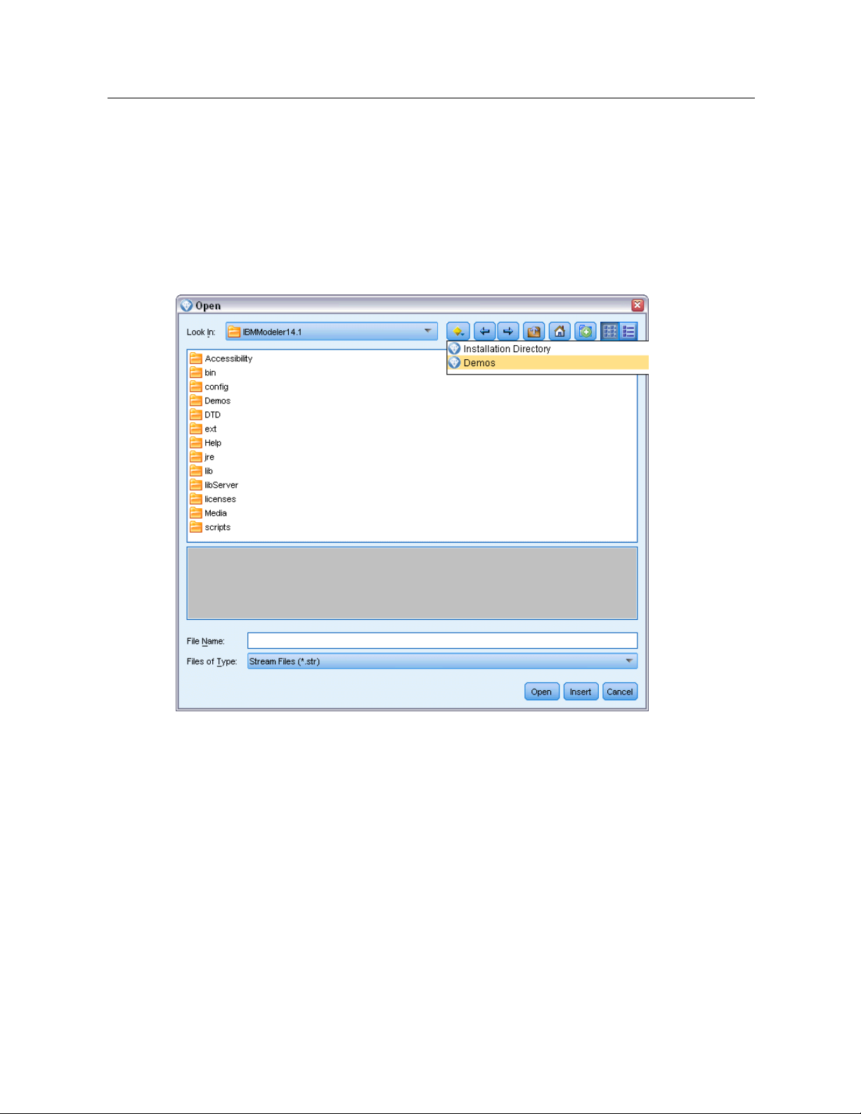
Demos Folder

The data ﬁles and sample streams used with the application examples are installed in the Demos folder under the product installation directory. This folder can also be accessed from the

SPSS Modeler 15

recent directories in the File Open dialog box.

Figure 1-1

Selecting the Demos folder from the list of recently-used directories

IBM

program gr oup on the Windows Start menu, or by clicking Demos on the list of

New Features

New and Changed Features in IBM SPSS Modeler 15

From this release onwards, IBM® SPSS® Modeler has the following editions.



IBM® SPSS® Modeler Professional



IBM® SPSS® Modeler Premium

features to those supplied by SPSS Modeler Professional.

The new features for these edit ions are described in the following sections.

New features in IBM SPSS Modeler Professional

The IBM® SPSS® Modeler Professional edition adds the following features in this release.

is the new name for the existing SPSS Modeler product.

is a sepa r ately-licensed product that provides additio nal

Chapter

GLMM modeling node.

that: the target is linearly related to the factors and covariates via a speciﬁed link function; the target can have a non-normal d is tribution; and the observations can be correlated. Generalized linear mixed models cover a wide variety of models, from simple linear regression to co mplex multilevel models for non-normal longitudinal data. For more information, see the topic New

Nodes in This Release on p. 10.

Support for maps in the Graphboard node.

number of map types. These include choropleths (wher e regions can be given different colors or patterns to indicate different values) and point overlay maps (where geospatial points are overlaid on the map).

IBM® SPSS® Modeler ships with several map ﬁle s, but you can use the Map Conversion Utility to convert your existing map shapeﬁles for use with the Graphboard Template Chooser.

Netezza Time Series and Generalized Linear nodes.

Netezza® Analytics in - database mining: Time Series and Generalized Linear. For more information, see the topic New Nodes in This Release on p. 10.

Netezza nodes enabled through Helper Applications.

nodes are now enabled in the same way as the other database modeling nodes.

Generalized linear mixed models (GLMMs) extend the linear model so

The Graphboard node now includes support for a large

Two new nodes are available for IBM®

The Netezza Analytics database modeling

Zooming in and out on the stream view.

from the standard size. This feature is particularly useful for gaining an overall view of a complex stream, or for minimizing the number of pages needed to pri nt a stream. For more information, see the topic Changing the icon size for a stream in Chapter 3 on p. 24.

It is now possible to scale the entire stream view up or down

Chapter 2

Default settings for database connections.

and Ora cle dat

abase connections, as we ll as those already supported for IBM DB2 InfoSphere

You can now specify default settings for SQL Server

Warehouse.

Stream properties and optimization redesign.

The Options tab on the Stream Properties dialog box has been redesigned to group the options into categories. The Optimizatio n options have also moved from User Options to Stream Properties. For more information, see the topic Setting

Options for Streams in Chapter 5 on p. 54.

Node execution timing.

You can now set an option to display individ ual execution times for the nodes in a stream. For more information, see the topic Viewing Node Execution Times in Chapter 5 on p. 67.

You can also set an option (time_ecode_execution_log) in the server conﬁguration ﬁle to record these execution times in the message log.

Stream parameters in SQL queries from Database source node.

You can now include SPSS Modeler

stream parameters in SQL queries that you enter in the Database source node.

Expression Builder supports in-database functions.

If a stream connects to a database through a Database source node and you use the Expression Builder with a downstream node, you can include in-database functions from the connected database directly in the expression you are building. For more in f ormation, see the t opic Selecting Functions in Cha pter 7 on p. 120.

IBM Cognos BI node enhancements.

The Cognos BI source node now supports importing C ognos

list reports as we ll as data, and additionally supports the use of parameters and ﬁlters.

For the Cognos BI source a nd export nodes, SPSS Modeler now automatically detects the version of IBM Cognos BI in use.

Enhancements to Aggregate node.

The Aggregate node n ow supports several new aggregation

modes for aggregate ﬁelds: median, count, variance, and ﬁrst and third quartiles.

Merge node supports conditional merge.

You can now perform input record merges that depend on satisfying a condition. You can specify the condition directly in the n ode, or build the conditio n using the Expression Builder.

Enhancements to in-database mining nodes for IBM DB2 InfoSphere Warehouse.

For in-database mining with IBM DB2 InfoSphere Warehouse, the ISW Clustering node now supports the Enhanced BIRCH algorithm in addition to demographic and Koho nen clustering. In addition, the ISW Associ ation node provides a choice of layout for non-transactional (tabular) data.

Table compression for database export.

When exporting to a database, you can now specify table compression options for SQL Server and Oracle database connections, as well as those already supported for IBM DB2 InfoSphere Warehouse.

Bulk loading for database export.

Additional help information is available for database bulk loading

using an external loader program.

New Features

SQL generation enhancements.

timestamp, an

d string data types, in additi on to integer and real. With IBM Netezza databases, the

The Aggregate node now supports SQL generation for date, time,

Sample node supports SQL generation for simple and complex sampling, and the Binn ing node supports SQL generation for all binning methods except Tiles.

In-database model scoring.

For I B M DB2 for z/OS, IBM Netezza and Teradata da tabases, it is possible to enable SQL pushback of many of the model nuggets to carry out model scoring (as opposed to in-database mining) within the database. To do this, you can install a scoring adapter into the database. When you publish a model for the scoring adapter, the model is enabled to use the user-deﬁned function (UDF) capabilities of the database to perform the scoring.

A new conﬁguration option, db_udf_enabled in options.cfg, causes the SQL generation option to generate UDF SQL by default.

New format for database connection in batch mode.

The format for specifying a database connection in batch mode has changed to a single argument, to be consistent with the way it is speciﬁed in scripting.

Enhancements to SPSS Statistics integration.

are available on the Syntax tab th r ough the

On the Statistics Output node, additional procedures

Select a dialog

button. The Regres sion submenu now supports Partial Least Squares regression, and there is a new Forecasting submenu with the following op tions: Spectral Analysis, Sequence Charts, Autocorrelations, and Cross-correlations. For mor e information, see the SPSS Statistics documentation.

The Syntax tab of the Statistics Output node also has a new option to generate a Statistics File source node for importing the data that results fr om running a stream containing the node. This is useful where a procedure writes ﬁelds such as scores to the active datas et in addition to displaying output, as these ﬁelds would otherwise not be visible.

Non-root user on UNIX servers.

If you have SPS S Modeler Server installed on a UNIX server, you can now install, conﬁgure, and start and stop SPSS Modeler Server as a non-root user without the need for a pr ivate password database.

Deployed streams can now access IBM SPSS Collaboration and Deployment Services model management features.

When a stream is deployed to IBM SPSS Collaboration and Deployment Services as a str eam, it can now use the same model management features as it could if deployed as a scenario. These features include evaluation, refresh, score, and champion/challenger.

Improved method of changing ODBC connection for SPSS Modeler stream and scenario job steps.

For stream and scenario job steps in IBM SPSS Collaboration and Deployment Services, changes to an ODBC connection and related logon credentials apply to all rela ted job steps. This means that you no longer have to change the job steps one by one.

Choice of execution branch in deployed streams.

For stream job steps in IBM SPSS Collaboration and Deployment Services, if the stream contains branches you can now choose one or more stream branches to execute.

Chapter 2

New features in IBM SPSS Modeler Premium

IBM® SPSS® Modeler Premium is a separately-licensed product that provides additional features to those supplied by IBM® SPSS® Modeler Professional. Previously, SPSS Mode ler Premi um included only IBM® SPSS® Modeler Text Analytics . The full set of SPS S Modeler Premium features is now as follows.



SPSS Modeler Text Analytics



IBM® SPSS® Modeler Entity Analytics



IBM® SPSS® Modeler Social Network Analysis

SPSS Modeler Text Analytics uses advanc ed linguistic technologies and Natural Language Processing (NLP) to rapidly process a large variety of unstructured text data, extract and organize the key concepts, and group these concepts into categories. Extracted concepts and categories can be combined with existing structured data, such as demographics, and applied to modeling using the full suite of IBM® SPSS® Modeler data mining tools to yield better and more focused decisions.

IBM SPSS Modeler Entity Analytics adds a complet ely ne w dimension to SPSS Modeler predictive analytics. Whereas predictive analytics attempts to predict future behavior from past data, entity analytics focuses on improving the coherence and consistency of current data by resolving identity conﬂicts within the records themselves. An identity can be that of an individual, an organization, an object, or any other entity for which ambiguity might exist. Identity resolution can be vital in a number of ﬁelds, including customer relationship management, fraud detection, anti-money laundering, and national and international security.

IBM SPSS Modeler Social Network Analysis transforms information about relationships into ﬁelds that characterize the social behavior of individuals and groups. Using data describing the relationships underlying social networks, IBM SPSS Modeler Social Network Analysis identiﬁes social leaders who inﬂuence the behavior of others in the network. In addition, you can determine which people are most affected by other network participants. By combining these results with other measures, you can create comprehensive proﬁles of individuals on which to base your predictive models. Models that inclu de this social information will perform better than models that do not.

Note: SPSS Modeler Professional must be installed before installing any of the SPSS Modeler Premium features.

New Nodes in This Release

IBM SPSS Modeler Professional

A generalized linear mixed model (GLMM) extends th e linear model so that the target can have a non-normal distribution, is linearly related to the factors and covariates via a speciﬁed link function, and so that the observations can be correlated. Generalized linear mixed models cover a wide variety of models, from simple linear regression to complex multilevel models for non-normal longitudinal data.

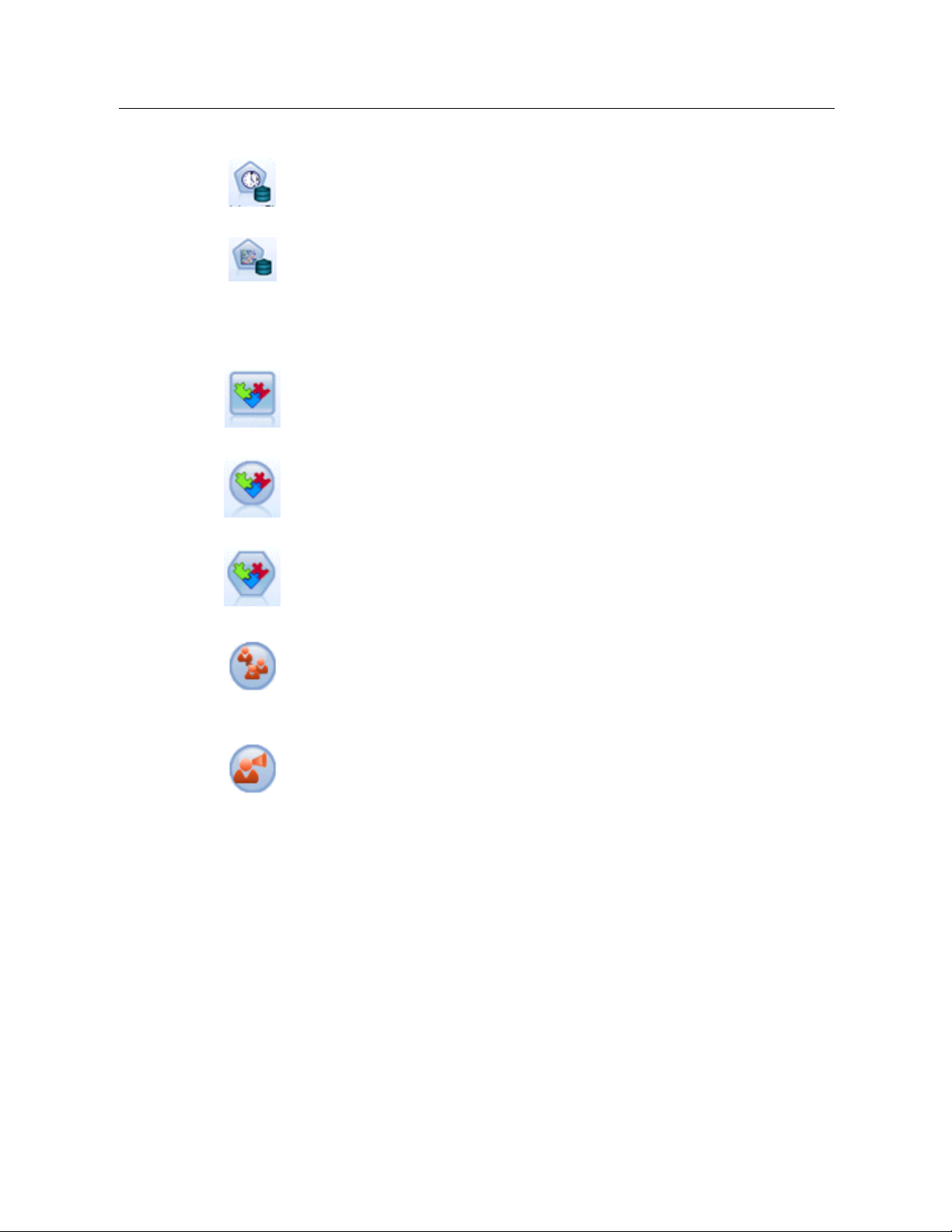
The Netezza Time Series node analyzes time series data and can predict future behavior from past events.

The Netezza Generalized Linear model expands the linear regression model so that the dependent variable is related to the predictor vari ables by means of a speciﬁed link function. Moreover, the model all ows for the dependent variable to have a non-normal distribution.

IBM SPSS Modeler Premium

The EA Export node is a terminal node that reads entity data from a data source and exports the data to a repository for the purpose of entity resolution.

New Features

The Entity Analytics(EA) source node reads the resolved entities from th e repository and passes th

is data to the stream for further processing, such as formatting into

a report.

The Streaming EA node compares new cases against the entity data in the repository.

The SNA Group Analysis node builds a model of a social net w ork based on input data about the social groupings within the network. This technique identiﬁes links between the group members, and analyzes the interactions within the groups to produce key performance indicators (KPIs). The KPIs can be used for purposes such as churn prediction, anomaly detection, or group leader identiﬁcation.

The SNA Diffusion Analysis node models the ﬂow of information from a group member to t heir social environment. A group member is assigned an initial weighting, which is propagated across the network as a gradually reducing ﬁgure. This process continues until each member of the network has been assigned a weighting relative to the original group member, according to the amount of information that has reached them. The individual member scores are then derived directly from these weightings. In this way, for examp l e, a service provider could identify customers that are at a higher risk of churn according to their relationship with a recent churner.

IBM SPSS Modeler Overview

Getting Started

As a data mining application, IBM® SPSS® Modeler offers a strategic approa ch to ﬁnding useful relationships in large data sets. I n contrast to more traditional statistical methods, you do not necessarily need to know what you are looking for when you start. You can explore y our data, ﬁtting different models and investigating different relationships, until you ﬁnd useful information.

Starting IBM SPSS Modeler

To start the application, cli ck:

Start > [All] Programs > IBM SPSS Modeler15 > IBM SPSS Modeler15

Chapter

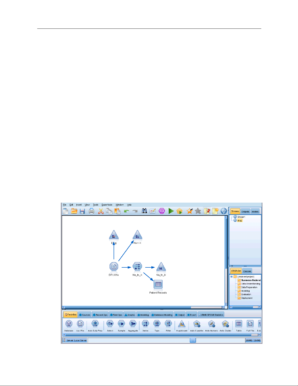
The main window is displayed after a few seconds.

Figure 3-1

IBM SPSS Modeler main application window

Launching from the Command Line

You can use the command li ne of your operating system to launch IBM® SPSS® Modeler as follows:

On a computer where IBM® SPSS® Modeler is installed, open a DOS, or command-prompt, window.

To launch the SPSS Modeler interface in interactive mode, type the modelerclient command followed by the re quired arguments; for example:

modelerclient -stream report.str -execute

The ava ilable arguments (ﬂags) allow you to connect to a se r ver, load streams, run scripts, or specify other parameters as needed.

Connecting to IBM SPSS Modeler Server

IBM® SPSS® Modeler can be run as a standalone application, or as a client connected to IBM® SPSS® Modeler Server directly or to an SPSS Modeler Server or server cluster through the Coordinator of Processes plug- in from IBM® SPSS® Collaboration and Deployment Services. The current connection status is displayed at the bottom left of the SPSS Modeler window.

Whenever you want to connect to a server, you can ma nually enter the server name to which you want to connect or select a name that you have previously deﬁned. How ever, if you have I B M SPSS Collaboration an d Deployme nt Services, you can search through a list of servers or server clusters fro m the Server Login dialog box . The ability to browse through the Statistics services running o n a network is made available through the Coordinator of Processes.

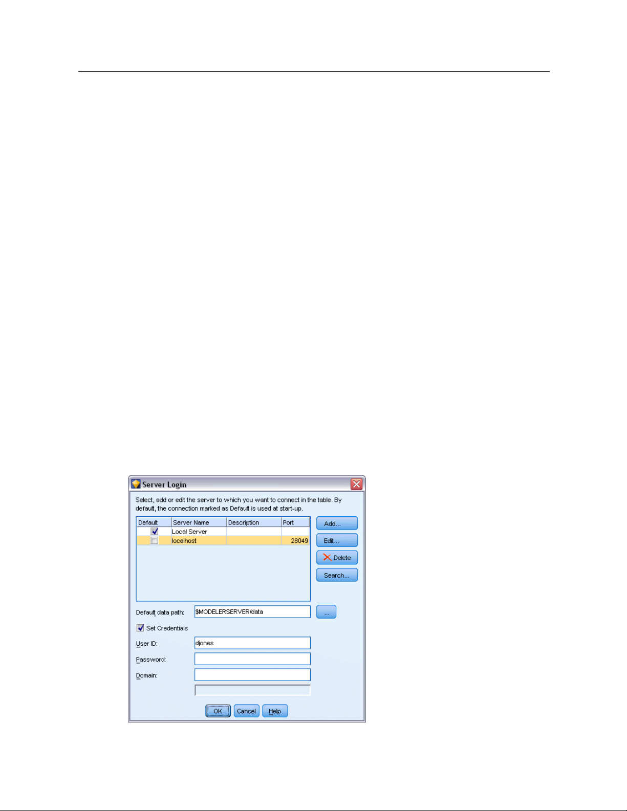
IBM SPSS Modeler Overview

Figure 3-2

Server Login dialog box

Chapter 3

To Connect to a Server

On the Tools menu, click

Server Login

. The Server Login dialog box opens. Alternatively,

double-click the connection status area of the SPSS Modeler window.

Using the dialog box, specify options to connect to the local server computer or select a connection from the table.



Click

AddorEdit

to add or edit a connection . For mor e information, see the topic Adding and

Editing the IBM SPSS Modeler Server Connection on p. 14.



Click

to acces s a server or server cluster in the Coordinator of Processes. For more information, s ee the topic Searching for Servers in IBM SPSS Collaboration and Deployment

Services on p. 16.

Server table.

This table c ontains the set of deﬁned server connections. The table displays the default connection, server name, description, and port number. You can manually add a new connection, as well as select or search for an existing connection. To set a particular server as the default conne ction, select the check box in the Default column in the table for the connection.

Default data path.

Specify a path used for data on the server com puter. C lick the ellipsis button

to browse to the required location.

Set Credentials.

Leave this box unchecked to enable the single sign-on feature, which attempts to log you in to the server using your local computer username and password details. If single sign-on is not possible, or if you check this box to disable single sign-on (for example, to log in to an administrator account), the following ﬁelds are enabled for you to enter your credentials.

User ID.

Password.

Domain.

Enter the user name with which to log on to the server.

Enter the passwo r d associa ted with the speciﬁed user name.

Specify the domain used to log on to the server. A domain name is required only when

the server computer is in a different Windows domain th an the client computer.

ClickOKto complete the connection.

To Disconnect from a Server

On the Tools menu, click double-click the con

Server Login

. The Server Login dialog box opens. Alternatively,

nection status area of the SPSS Modeler window.

(...)

In the dialog box, select the Local Server and clickOK.

Adding and Editing the IBM SPSS Modeler Server Connection

You can manually edit or add a server connection in the Server Login dialog box. By clicking Add, you can access an empty Add/Edit Server dialog box in which you can enter server connection details. By selecting an existing connection and clicking Edit in the Server Login dialog box, the Add/Edit Server dialog box opens with the details for that connection so that you can make any changes.

IBM SPSS Modeler Overview

Note: You cannot edit a server connection that was added f r om IBM® SPSS® Collaboration and Deploymen

t Services, since the name, port, and other deta ils are deﬁned in IBM SPSS

Collaboration and Deployment Services.

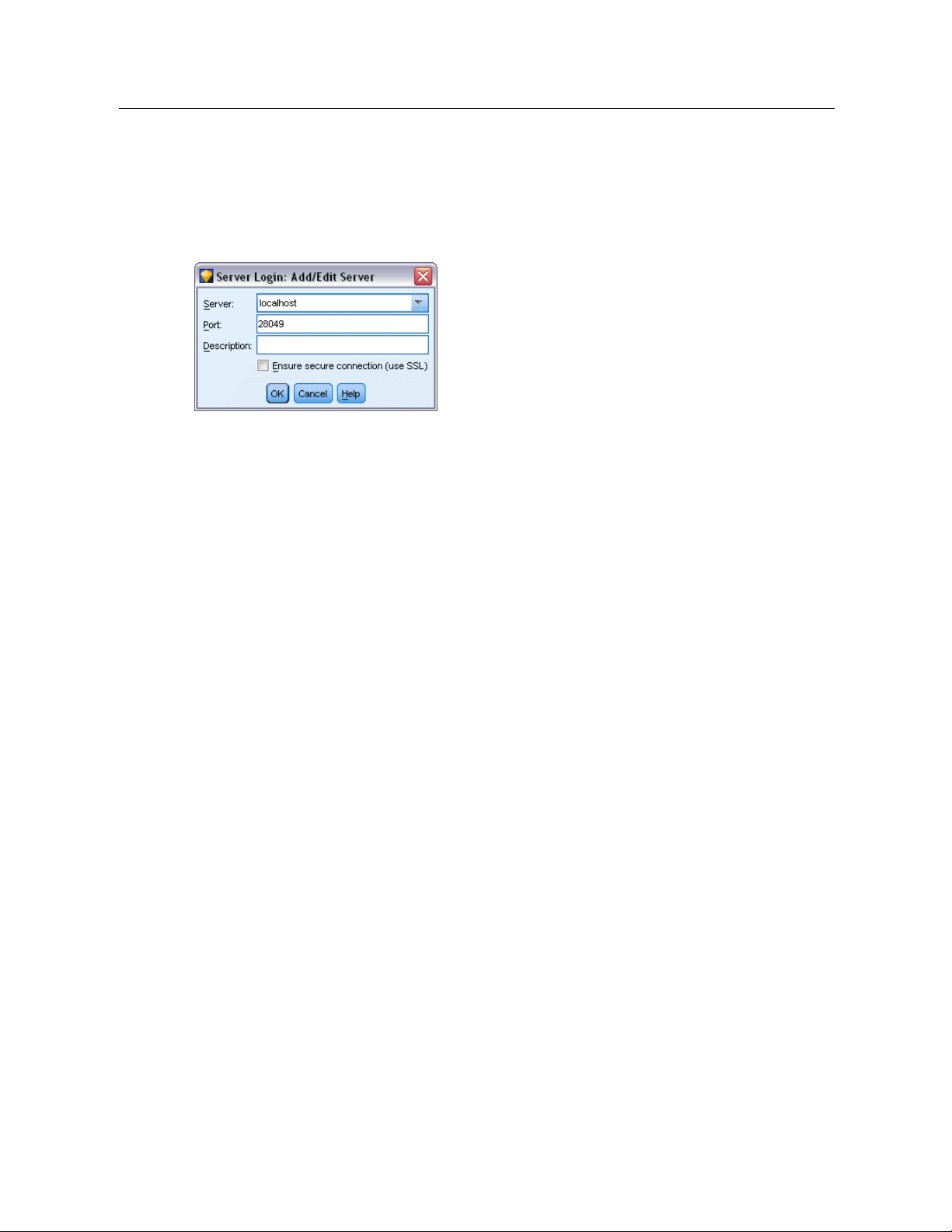
Figure 3-3

Server Login

Add/Edit Server dialog box

To Add Server Connections

On the Tools menu, click

In this dialog box, click

Enter the server connection details and clickOKto save the connection and retu r n to the Server

Server Login

Add

. The Server Login Add/Ed it Server dialog box opens .

. The Server Login dialog box opens.



Server.

Specify an ava ilable server or select one from the list. The server computer can be

identiﬁed by an alphanumeric name (for example, myserver) or an IP address assigned to the server computer (for example, 202.123.456.78).



Port.

Give the port number on which the server is listening. If the d efault does not work, ask

your system administrator for the corre ct port number.



Description.



Ensure secure connection (use SSL).

Enter an optional description for this server con ne ction.

Speciﬁes whether an SSL (Secure Sockets Layer) connection should be used. SSL is a commonly used protocol for securing data sent over a network. To use this feature, SSL must be enabled on the server hosting IBM® SPSS® Modeler Server. If necessary, contact your local administrator for details.

To Edit Server Connections

On the Tools menu, click

In this dialog box, select the connec tion you want to ed it and then click

Server Login

. The Server Login dialog box opens.

Edit

. The Server Login

Add/Edit Server dialog box opens.

Change the server connection details and clickOKto save the changes and return to the Server Login dialog box.

Chapter 3

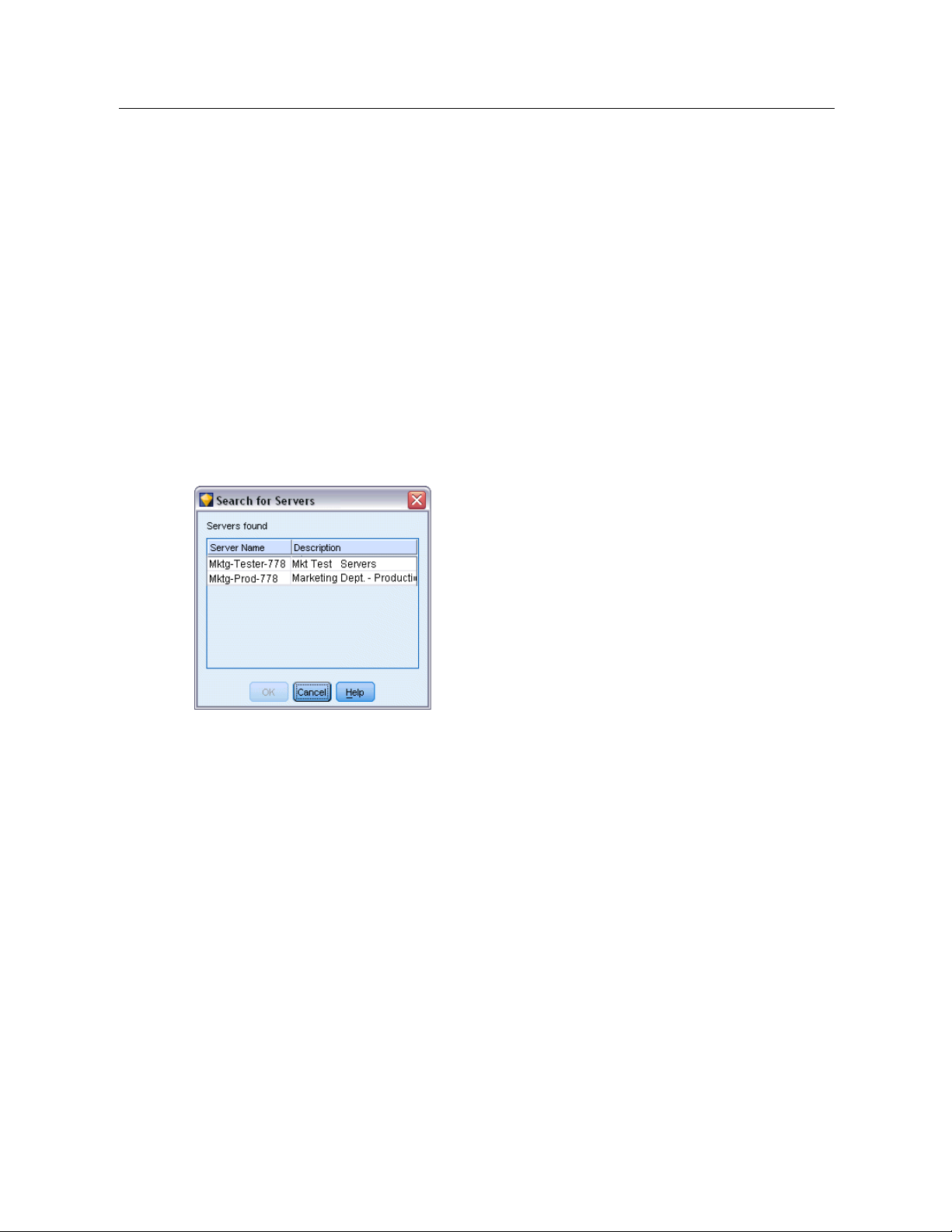
Searching for Servers in IBM SPSS Collaboration and Deployment Services

Instead of entering a server connection manually, you can select a server or server cluster available on the network through the Coor dinator of Processes, available in IBM® SP SS® Collab oration and Deployment Services. A server cluster is a group of servers from which the Coordinator of Processes determines the server best suited to respond to a processing request.

Although you can ma nually add servers in the Ser ver Login dialog box, searching for available servers lets you connect to servers without requiring that you know the correct server name and port number. This information is autom atically provided. However, you still need the correct logon information, such as username, domain, and pass word.

Note: If you do not have access to the Coordinator of Proc esses capability, you can still manually enter the server name to which you want to connect or select a name that you have previously deﬁned. For more information, see the topic Adding and Editing the IBM SPSS Modeler Server

Connection on p. 14.

Figure 3-4

Search for Servers dialog box

To search for servers and clusters

On the Tools menu, click

In this dialog box, click logged on to IBM SPSS Collaboration and Deployment Services when you attempt to browse the Coordinator of Processes, you will be prompted to do so. For more information, see th e topic Connecting to the Repository in Chapter 9 on p. 161.

Select the server or server cluster from th e list.

ClickOKto close the dialog box and add this connection to the table in the Server Login dialog box.

Changing the Temp Directory

Some operations perfor med by IBM® SPSS® Modeler Server may require temporary ﬁles to be created. By default, IBM® SPSS® Modeler uses the system temporary directory to create temp ﬁles. You can alter the location of the temporary directory using the following steps.

Create a new directory called spss and subdirectory called servertemp.

Server Login

to open the Search for Ser ve r s dialog box. If you are not

. The Server Login dialog box opens.

Edit options.cfg, located in the /conﬁg directory of y our SPSS Modeler ins tallation directory. Edit the temp_dire

After doing this, you must restart the SPSS Modeler Server service. You can do this by clicking the

Services

ctory parameter in this ﬁle to read:

tab on your Windows Control Panel. Just stop the service and then start it to activate

the changes you made. Restarting the m achine will also restart the service.

All temp ﬁles will now be written to this new directory.

Note: The most common error when you are attempting to do this is to use the wrong type of slashes. Because of SPSS Modeler’s UNIX history, forward slashes are used.

Starting Multiple IBM SPSS Modeler Sessions

If you need to launch more than one IBM® SPSS® Modeler s ession at a time, you must make some changes to your IBM® SPSS® Modeler and Windows settings. For example, you may need to do th is if you have two separate se r ver license s and want to run two streams against two different servers from the same client machine.

To enable multiple SPSS Modeler sessions:

IBM SPSS Modeler Overview

temp_directory, "C:/spss/servertemp"

Click:

Start > [All] Programs > IBM SPSS Modeler15

On the IBM SPSS Modeler15 shortcut (the one with the icon), right-click and select

In the

Target

text box , add

In Windows Explorer, select:

Tools > Folder Options...

On the File Types tab, select the SPSS Modeler Stream option and click

In the Edit File Type dialog box, select

In the

Application used to perform action

-noshare

to the end of the string.

Open with SPSS Modeler

text box, add

IBM SPSS Modeler Interface at a Glance

At each point in the data mining proce ss, IBM® SPSS® Modeler’s easy-to-use interface invites your speciﬁc business e xpertise. Modeling algorithms, such as prediction, classiﬁcation, segmentation, and association detection, ensure powerful and accurate models. Model results can easily be deployed a nd read into databases, IBM® SPSS® Statistics, and a wide variety of other applications.

-noshare

and click

before the

Advanced

Edit

-stream

Properties

argument.

Working with SPSS Modeler is a three-step process of working with data.



First, you read data into SPSS Modeler.



Next, you run the data through a series of manipulations.



Finally, you send the data to a destination.

Chapter 3

This sequ ence of operations is known as a data stream because the data ﬂows record by record from the sourc

e through each manipulation and, ﬁnally, to the destination—either a model or

type of data output.

Figure 3-5

A simple stream

IBM SPSS Modeler Stream Canvas

The stream canvas is the largest area of the IBM® SPSS® Modeler window and is where you will build and manipulate data streams.

Streams are created by drawing diagrams of data operations relevant t main canvas in the interface. Each operation is represented by an icon or node, and the nodes are linked together in a stream representing the ﬂow of data through each operation.

You can work with multiple streams at one time in SPSS Modeler, either i canvas or by opening a new stream canvas. During a sessi on, streams are stored in the Streams manager, at the upper right of the SPSS Modeler window.

o your business on the

n the same stream

Nodes Palette

Most of the data and modeling tools in IBM® SPSS® Modeler reside in the Nodes Palette, acr oss the b ottom o f the window below the stream canvas.

For example, the Record Ops palette tab contains nodes that you can use to perform operations on the data records, such as selecting, merging, and appending.

To add nodes to the canvas, double-click icons from the Nodes Palette or drag and drop them onto the canvas. You then connect them to create a stream, representing the ﬂow of data.

Figure 3-6

Record Ops tab on the nodes palette

Each palette tab contains a collection of related nodes used for different p hases of stream operations, such as :



Sources.



Record Ops.

appending.

Nodes bring data into SPSS Modeler.

Nodes perform operations on data records, such as selecting, merging, an d

IBM SPSS Modeler Overview



Field Ops.

Nodes perform operations on data ﬁelds, such as ﬁltering, deriving new ﬁelds, and

determining the measurement level for given ﬁelds.



Graphs.

Nodes graphically display data before and after modeling. Graphs include plots,

histograms, web nodes, and evaluation charts.



Modeling.

des use the modeling algorithms available in SPSS Modeler, such as neural nets ,

decision trees, clustering algorithms, and data sequencing.



Database Modeling.

Nodes use the modeling algorithms available in Microsoft SQL Server,

IBM DB2, and Oracle database s.



Output.

Nodes produce a variety of output for d ata, charts, and model results that can be

viewed in SPSS Modeler.



Export.

es prod uce a variety of output that can be viewed in external applications, such

Nod

as IBM® S PSS® Data Collection or Excel.



SPSS Statistics.

Nodes import data from, or export data to, IBM® SPSS® Stat is tics, as well as

running SPSS Statistics procedures.

As you become more familiar with SPSS Modeler, you can customize the palette contents for your own use. For more information, see the topic Customizing the Nodes Palette in Chapter 12 on p. 223.

Located below the Nodes Palette, a report pane provides feedback on the progress of various operations, such as when data is being read into t he data stream. Also located below the Nodes Palette, a status pane provides info r mation on what the application is currently doing, as well as indications of when user feedback is required.

IBM SPSS Modeler Managers

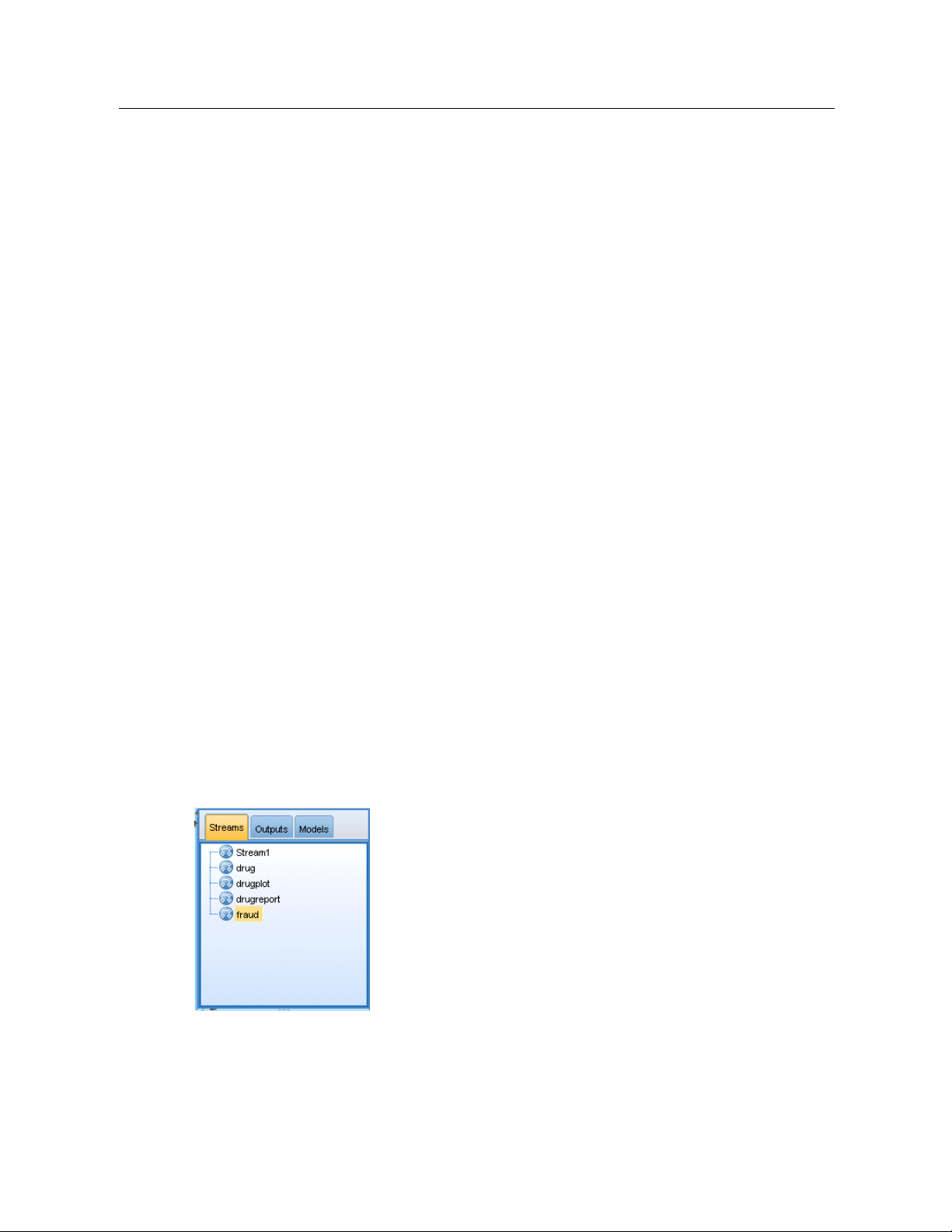
At the top right of the window is the managers pane . This has three tabs, which are used to manage streams, output and models.

You can use the Streams tab to open, rename, save, and dele te the streams created in a session.

Figure 3-7

Streams tab

The Outputs tab contains a variety of ﬁles , such as graphs and tables, produced by stream operations in IBM® SPSS® Modeler. You can display, save, rename, and close the tables, graphs, and reports listed on this tab.

Chapter 3

Figure 3-8

Outputs tab

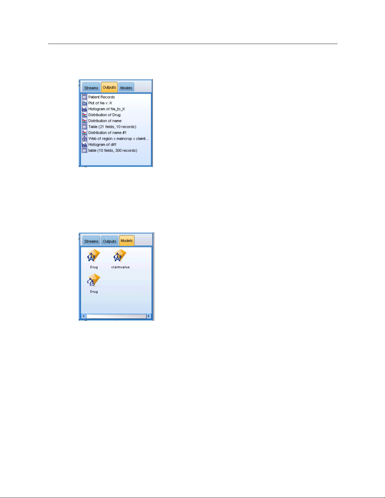
The Models tab is the most powerful of the manager tabs. This tab contains all model nuggets, which contain the models generated in SPSS Modeler, for the current session. These models can be browsed directly from the Models tab or added to the stream in the c anvas.

Figure 3-9

Models tab containing model nuggets

IBM SPSS Modeler Projects

On the lower right side of the window is the project pane, used to create and manage data mining projects (groups of ﬁles related to a data mining task). There are two ways to view projects you

in IBM® SPSS® Modeler—in the Classes view and the CRISP-DM view.

create

The CRISP-DM tab provides a way to organize projects according to the Cross-Industry Standard Process for Data Mining, an industry-proven, nonproprietary methodology. For both

enced and ﬁrst-time data miners, using the CRISP-DM tool will help you to better o rganize

experi and communicate your efforts.

IBM SPSS Modeler Overview

Figure 3-10

CRISP-DM view

The Classes tab provides a way to organize your work in SPSS Modeler categorically—by the types of objects you create. This view is useful when taking inventory of data, streams, and models.

Figure 3-11

Classes view

IBM SPSS Modeler Toolbar

At the top of the IBM® SPSS® Modeler window, you will ﬁnd a toolbar of icons that provides a number of useful functions. Following a r e the toolbar buttons and their functions.

Create new stream Open stream

Save stream

Print current stream

Chapter 3

Cut & move to clipboard Copy to clipboard

Paste selection Undo last action

Redo Search for nodes

Edit stream properties Preview SQL generation

Run current stream

Stop stream (Active only while stream is running)

Zoom in (SuperNodes only) Zoom out (SuperNodes only)

No markup in stream

Hide stream markup (if any) Show hidden stream markup

Open stream in IBM® SPSS® Modeler Advantage

Run stream selection

Add SuperNode

Insert comment

Stream markup consists of stream comments, model links, and scoring branch indications.

For mor e information on stream comments , see Adding Comments and Annotations to Nodes

and Streams on p. 78.

For more i

nformation on scoring branch indications, see The Scoring Branch on p. 188.

Model links are described in the IBM SPSS Modeling Nodes guide.

Customizing the Toolbar

You can change various aspects of the toolbar, such as:



Whether it is displayed



Whether the icons have tooltips available



Whether it uses large or small icons

To turn the toolbar display on and off:

On the main menu, click:

View > Toolbar > Display

To change the tooltip or icon size settings:

On the main menu, click:

View > Toolbar > Customize

IBM SPSS Modeler Overview

Click

Show Too

lTipsorLarge Buttons

as required.

Customizing the IBM SPSS Modeler Window

Using the dividers between vario us portions of the IBM® SPSS® Modeler interface, you can resize or close tools to meet your preferen ces. For example, if you are working with a large stream, you can use the small arrows located on each divider to close the nodes palette, managers pane, and project pane. This maximizes the stream canvas, providing enough work space for large or multiple streams.

Alternativ

ely, on the View menu, click

these items on or off.

Nodes Palette,Managers

, or

Project

to turn the dis play of

Chapter 3

Figure 3-12

Maximized stream canvas

As an alternative to closing the nodes palette, and the managers and project panes, you can use the stream canvas as a scrollable page by moving vertically and horizontally with the scrollbars a t the side and b ottom of the SPSS Mode ler window.

You can also co ntrol the display of screen markup, which consists of stream comments, model

and scoring branch indications. To turn this display on or off, click:

links,

View > Stream Markup

Changing the icon size for a stream

You can



You can standard icon size.

change the size of the s tream icons in the following ways.

Through a stream property settin g

gh a p op-up menu in the stream

Throu

Using the keyboard

scale the entire stream view to one of a nu mber of sizes between 8% and 200% of the

Figure 3-13

Changing the icon size

IBM SPSS Modeler Overview

To scale the entire stream (stream properties method)

From the main menu, choose

Tools > Stream Properties > Options > Layout.

Choose the size y ou want from the Icon Size menu.

Click

Apply

to see the result.

ClickOKto save the change.

To scale the entire stream (menu method)

Right-click the stream background on the canvas.

Choose

Icon Size

and select th e size you want .

To scale the entire stream (keyboard method)

Press Ctrl + [-] on the main keyboard to zoom out to the next smaller size.

Press Ctrl + Shift + [+] on the main key board to zoom in to the next larger size.

This feature is particularly useful for gaining an overall view of a complex stream. You can also use it to minimize the number of pages needed to print a stream.

Chapter 3

Using the Mouse in IBM SPSS Modeler

The most common uses of the mouse in IBM® SPSS® Modeler include the follow ing:



Single-click.

pop-up m enus,

Use either the right or left mouse button to select options from m enus, open

and ac cess vario us other standard controls and options. Click and hold the

button to move and drag nodes.



Double-click.

Double-click using the left mouse button to place nodes on the stream canvas

and edit existing nodes.



Middle-click.

Click the middle mouse bu tton an d drag the cursor to connect nodes on the stream canvas. Double-click the middle mouse button to disconnect a node. If you do not have a three-button mouse, you can simulate this feature by pressing the Alt key while clicking and dragging the mouse.

Using Shortcut Keys

Many visual progra mming operations in IBM® SPSS® Modeler have s hortcut keys associated with them. For example, you can delete a node by clicking the node and pressing the Delete key on your keyboard. Likewise, you can quickly save a stream by pr essing the S ke y while holding down th e Ctrl key. Control commands like this one are indicated by a combination of Ctrl and another key—for example, Ctrl+S.

There are a number of shortcut keys used in standard Windows operations, such as Ctrl+X to cut. These shortcuts are supported in SPSS Modeler along with the following application-speciﬁc shortcuts.

Note: In some cases, old shortcut keys us ed in SPSS Modeler conﬂict with standard Windows shortcut keys. These old shortcuts are supported with the addition of the Alt key. For example, Ctrl+Alt+C can be used to toggle the cache on and off.

Table 3-1

Supported shortcut keys

Shortcut Key

Ctrl+A Select all Ctrl+X Cut Ctrl+N Ctrl+O Ctrl+P Print Ctrl+C Ctrl+V Ctrl+Z Undo Ctrl+Q Select all nodes down stream of the selected node Ctrl+W Deselect all downstream nodes (toggles with Ctrl+Q) Ctrl+E Run from selected node Ctrl+S Alt+Arrow

keys Shift+F10 Open the pop-up menu for the selected node

Function

New stream Open stream

Copy Paste

Save current stream Move selected nodes on the stream canvas in the direction

of the arrow used

Printing

IBM SPSS Modeler Overview

Table 3-2

Supported shortcuts for old hot keys

Shortcut Key

Ctrl+Alt+D Duplicate node Ctrl+Alt+L Load node Ctrl+Alt+R Rename node Ctrl+Alt+U Create User Input node Ctrl+Alt+C Toggle cache on/off Ctrl+Alt+F Flush cache Ctrl+Alt+X Expand SuperNode Ctrl+Alt+Z Zoom in/zoom out Delete Delete node or connection

Function

The fol lowing ob jects can be printed in IBM® SPSS® Modeler:



Stream diagrams



Graphs



Tables



Reports (from the Report node and Project Reports)



Scripts (from the stream propertie s, Standalone Script, or SuperNode script dialog boxes)



Models (Model browsers, dialog box tabs with current focus, tree viewers)



Annotations (using the Annotations tab for output)

To print an object:



To print without previewing, click the Print button on the toolbar.



To set up the page before printing, select



To preview before printing, select



To view the standard print dialog box w ith options for selecting printers, and specifying

appearance options, select

Automating IBM SPSS Modeler

Since a dvanced data mining can be a co mplex and sometimes lengthy process, IBM® SPSS® Modeler includes several ty pes of coding and automation support.



Control Language for Expression Manipulation (CLEM) is a language for an alyzing

and manipulating the data that ﬂows along SPSS Modeler streams. Data miners use CLEM extensively in stream operations to perform tasks as simple as deriving proﬁt from cost and

Page Setup

Print Preview

from the File menu.

Chapter 3

revenue data or as complex as tran sforming web log data into a set of ﬁelds and records with usable information. For more in f ormation, see the topic About CLEM in Chapter 7 on p. 105.



Scripting is a powerful tool for automating pro cesses in the user interface. Scripts can

perform the same kinds of actions that users perform with a mouse or a keyboard. You can set options for n odes and perform derivations using a subset of CLEM. You can also spec ify output and manipulate generated models.

Understanding Data Mining

Data Mining Overview

Through a variety of techniques, data mining identiﬁes nuggets of information in bodies of data. Data m ining extracts information in such a way that it can be used in areas such as decision support, pred iction, forecasts, and estimation. Data is often vol little direct usefulness in its raw form. It is the hidden information in the data that has value.

In data mining, success comes from combining your (or your expert’s) knowledge of the data with advanced, active analysis techniques in which the com pu relationships and features in the data. The process of data mining generates models from historical data that are later used for predictions, pattern detection, and more. The technique for building these models is called machine learning or modeling.

Modeling Techniques

Chapter

uminous but of low value and with

ter identiﬁes the underlying

IBM® SPSS® Modeler includes a number of machine-learning and modeling technologies, which can be roughly grouped according to the types of problems the y are intended to solve.



Predictive modeling method s include decision trees, neural networks, and statistical models.



Clustering models focus on identifying groups of similar records and labeling the records

according to the group to which they belong. Clustering methods include Kohonen, k-means, and TwoStep.



Association rules associate a particular conclusion (such as the purchase of a particular

product) with a set of conditions (the purchase of several other products).



Screening models can be used to screen d ata to locate ﬁelds and records that are most likely to

be of interest in modeling and identify outliers that may not ﬁt known patterns. Available methods include feature selection and anomaly detection.

Data Manipulation and Discovery

SPSS Modeler also includes many facilities that le t you apply your expertise to the data:



Data manipulation.

data into meaningful subsets. Data from a variety of sources can be merged and ﬁltered.



Browsing and visualization.

an initia l audit including graphs and statistics. Advanced visualization includes interactive graphics, which can be exported for inclusion in project reports.



Statistics.

IBM® SPSS® Statistics can also be used within SPSS Modeler.



Hypothesis testing.

Conﬁrms suspected relationships between variables in the data. Statistic s from

Constructs new data items derived from existing ones and breaks down the

Displays aspects of the data using the Data Audit node to perform

Constructs models of how the data behaves and veriﬁes these models.

Chapter 4

Typically, you will use these faci lities to identify a promising set of attributes in the data. These attributes ca

n then be fed to the modeling techniques, which will attempt to identify underlying

rules and relationships .

Typical Applications

Typical applications of data mining techniques include the following:

Direct mail.

Determine which demograp hic groups have the highest response rate. Use this

information to maximize the response to fu ture mailings.

Credit scoring.

Human resources.

Use an individual’s credit history to make credit decisions.

Understand past hiring practices and create decision rules to streamline the

hiring process.

Medical research.

Create decision rules tha t suggest appropriate procedures based on medical

evidence.

Market analysis.

Determine which variables, such as geography, price, and customer

characteristics, are associated with sales.

Quality control.

Analyze data from product manufacturing and identify variables determining

product defects.

Policy studies.

Use surv ey data to for mulate polic y by applying decision rules to select the most

important variables.

Health care.

User surveys and clinical data can be combined to discover variables that contribute

to health.

Terminology

The terms attribute, ﬁeld, and variable refer to a single data item common to all cases under consideration. A collection of attribute values that refers to a speciﬁc case is called a record, an example, or a case.

Assessing the Data

Data mining is not likely to be fruitful unless the data you want to use meets certain criteria. The following sections present some of the asp ects of the data and its application that you should consider.

Ensure that the data is available

This ma y seem obvious, but be aware that although data might be available, it may not be in a form that can be used easily. IBM® SPSS® Modeler can import data from databa ses (through ODBC) o r from ﬁles. The data, however, might be held in some other form on a machine tha t cannot be directly accessed. It will need to be downloaded or du mped in a suitable form bef ore it can be used. It might be scattered among different databases a nd sources and need to be pulled

Understanding Data Mining

together. It may not even be online. If it exists only on paper, data entry will be required before you can begin d

Check whether the data covers the relevant attributes

ata mining.

The object of data mining is to identify relevant attributes, so including this check may seem odd at ﬁrst. It is very useful, however, to look at what data is available and to try to identify the likely relevant factors that are no t recorded. In trying to predict ice cream sales, for example, you may have a lot of information about retail outlets or sales history, but you may not have weather and t emperature information, which is likely to play a signiﬁcant role. Missing attributes do not necessarily mean that data mining will not produce useful results, but they can limit the accuracy of resulting predictions.

A qu ick way of assessing the situation is to perform a comprehensive audit of your data. Before moving on, consider attaching a Data Audit node to your data source and running it to generate a full report.

Beware of noisy data

Data often contains errors or may contain subjective, and therefore variable, judgments. These phenomena are collectively referred to as noise. Sometimes noise in data is normal. There may well be underlying rules, but they may not hold for 100% of the cases.

Typically, the more noise there is in data, the more difﬁcult it is to get accurate results. However, SPSS Modeler’s machine-learning methods are able to handle noisy data and have been used successfully on data sets containing almost 50% noise.

Ensure that there is sufficient data

In data mining, it is not necessarily the size of a data set that is important. The representativeness of the data set is far more signiﬁcant, together with its coverage of possible outcomes and combinations of variable s.

Typically, the more attributes that are considered, the more records that will be needed to give representative covera ge.

If the data is representative and there are general underlying rules, it may well be that a data sample of a few thousand (or even a f ew hundred) records will give equally good results as a million—and you will get the results more quickly.

Seek out the experts on the data

In many cases, you will be working on your own data and will therefore be highly familiar with its content and meaning. However, if you a r e worki ng on data for another department of your organization o r for a client, it is highly desirable th at you have access to experts who know the data. They can guide you in the identiﬁcation of relevant attributes and can help to interpret the results of data mining, distinguishing the true nuggets of information from “fool’s gold,” or artifacts caused by anomalies in the data sets.

Chapter 4

A Strategy for Data Mining

As with most business endeavors, data mining is much more effective if done in a planned, systematic way. Even with cutting-edge data mining tools, such as IBM® SPSS® Modeler, the majority of the work in data mining requires a knowledge ab le business analyst to keep the pr ocess on track. To guide your planning, answer the following questions:



What substantive problem do you want to solve?



What data sources a r e available, and what parts of the data are relevant to the current problem?



What kind of prep rocessing and data cleaning do yo u need to do before you start mining

the data?



What data mining technique(s) will you use?



How w ill you evaluate the results of the data mining analysis?



How will you get the most out of the information you obtained from data mining?

The typical data mining process can become com plicated very quickly. There is a lot to k eep track of—complex business pr oblems, multiple data sources, varying data quality across data sources, an array of data mining techniques, different ways of measuring data mining success, and so on.

To stay on track, it helps to have an explicitly deﬁned proces s model for data mining. The process model helps you answer the questions listed earlier in this section, and makes sure the important po ints are addressed. It serves as a data mining road map so that you will not lose your way as you dig into the complexities of your data.

The data mining process suggested for use with SPSS Modeler is the Cross-Industry Standard Process for Data Mining (CRISP-DM). As you can tell from t he name, this model is designed as a general mode l that can be applied to a wide variety of industries and business problems.

The CRISP-DM Process Model

The genera mining. The six phases ﬁt together in a cyclical process d esigned to incorporate data mining into your larger business practices.

l CRISP-DM process model includes six phases that addres s the main issues in data

Understanding Data Mining

Figure 4-1

CRISP-DM process model

The six phases include:



Business understanding.

This is perhaps the most important phase of data mining. Business understanding includes d etermining business objectives, assessing the situation, determining data mining goals, and producing a project plan.



Data understanding.

Data provides the “raw materials” of data mining. This phase addresses the need to understand what yo ur data resources are and the characteristics of those resources. It includes collecting initial data, describing data, exploring data, and verifying data quality. The Data Audit node available from the Output nodes palette is an indispensable tool for data understanding.



Data preparation.

After cataloging your data res ources, you will need to prepare your data for mining. Preparations include selecting, cleaning, constructing, integrating, and formatting data.



Modeling.

This is, of course, the ﬂashy part of data mining, where sophisticated analysis methods are used to extract information from the data. This phase involves selecting modeling techniques, generating test designs, and building and assessing models.



Evaluation.

Once you have chosen your models, you are ready to evaluate how the data min ing results can h elp you to achieve your busine ss obje ctives. Elements of this phase include evaluating results, reviewing the data mining process, and determining the next steps.



Deployment.

Now that you have invested all of this effort, it is time to reap the beneﬁts. This phase focuses on integrating your new knowledge into your everyday business processes to solve your original business problem. This phase includes plan deployment, monitoring and maintenance, producing a ﬁnal report, and reviewing the project.

There are some key points in this process model. First, while there is a general tendency for the process to ﬂow th r ough the steps in the order outlined in the previous paragraphs, there are also a number of places where the phases inﬂuence each other in a nonlinear way. For example, data preparation usually precedes modeling. However, decisions made and information gathered during the modeling phase can often lead you to rethink parts of the data prepa r ation phase, which can then present new modelin g issues. The two phases feed back on each other until bo th phases

Chapter 4

have been resolved adequately. Similarly, the evaluation phase can lead y ou to reevaluate your original busi

ness understanding, and you may decide that you have been trying to answer the wrong question. At this point, you can revise your business understanding and proceed through the rest of the process again with a better target in mind.

The second ke

y point is the iterative nature of data mining. You will rarely, if ever, simply plan a data mining project, complete it, and then pack up your data and go home. Data mining to address your customers’ demands is an ongoing endeavor. The knowledge gained from one cycle of data minin

g will almost invariably lead to new questions, new issues, and new opportunities to identify and meet you r customer s’ needs. Those new questions, issues, and opportunities can usually be addressed by mining your data once again. This process of mining and identifyin g new opportunit

ies shou ld become part of the way you think about you r business and a cornerstone of

your overall business strategy.

This introduction provides only a brief overview of the CRISP-DM process model. For

complete de



The CRISP-DM Guide, which can be accessed along with o ther documentation from the

tails on the model, consult the following resources:

\Documentation folder on the installation disk.



The CRISP-DM Help system, available from the Start menu or by clicking

CRISP-DM Help

the Help menu in IBM® SPSS® Modeler.

Types of Models

IBM® SPSS® Modeler offers a variety of modeling methods taken from machine learning, artiﬁcial intelligence, and statistics. The methods available on the Modeling palette allow you to derive new information from your data and to develop predictive models. Each method has certain strengths and is best suited for parti cular types of problems.

The SPSS Modeler Applications Guide provides examples for many of these methods, along

with a general introduction to the modeling process. This guide is available as an online tutorial, and also in PDF format. For more information, see the topic Application Examples in Chapter 1 on p. 5.

Modeling methods are divided into three categories:



Classiﬁcation



Association



Segmentation

Classification Models

Classiﬁcation models use the values of one or more input ﬁelds to predict the value of one or more output, or target, ﬁelds. Some examples of these techniques are: decision trees (C&R Tree, QUEST, CHAID and C5.0 algorithms), regression (linear, logistic, generalized linear, and Cox regression algorithms), neural networks, support vector machines, and Bayesian networks.

Classiﬁcation models helps organization s to predict a known result, such as whether a customer will buy or leave or whether a transaction ﬁts a known pattern of fraud. Modeling techniqu es include machine learning, rule induction, subgroup identiﬁcation, statistical m ethods, and multiple model generation.

Classiﬁcation nodes

Understanding Data Mining

The Auto Classiﬁer node creates and compares a number of different models for binary outcomes (yes or no, churn or do not churn, and so on), allowing you to choose the best approach for a given analysis. A number of modeling algorithms are supported, making it possible to select the methods you want to use, the speciﬁc options for each, and the criteria for comparing the results. The node generates a set of models based on the speciﬁed options and ranks the best candidat es according to the criteria you specify.

The Auto Numeric node estimates and compares models for continuous numeric range outcomes using a number of d i fferent methods. The node works in the same manner as the Auto Classiﬁer node, allowing you to choose the algorithms to use and to experiment wit h multiple combinations of options in a single modeling pass. Supported algorithms include neural networks, C&R Tree, CHAID, linear regression, generalized linear reg res sion, and support vector machines (SVM). Models can be compared based on correlation, relative error, or number of variables used.

The Classiﬁcation and Regression (C&R) Tree node generates a decision tree that allows you to predict or classify future observations. The method uses recursive partitioning to split the training r ecords into segments by minimizing the impurity at each step, where a node in the tree is considered “pure” if 100% of cases in t he node fall into a speciﬁc category of the target ﬁeld. Target and input ﬁelds can be numeric ranges or categorical (nominal, ordinal, or ﬂags); all splits are binary (only two subgroups).

The QUEST node provides a binary classiﬁcation method for building decision trees, designed to reduce t he processing time required for large C&R Tree analyses while also reducing the tendency found in classiﬁcation tree methods to favor inputs that allow more splits. Input ﬁelds can be numeric ranges (continuous), but the target ﬁeld must be categorical. All splits are binary.

The CHAID node generates decision tre es using chi-square statistics to identify optimal splits. Unlike the C&R Tree and QUEST nodes, CHAID can g enerate nonbinary trees, meaning that some splits have more than two branches. Target and input ﬁelds can be numeric range (continuous) or categorical. Exhaustive CHAID is a modiﬁcation of CHAID that doe s a more thorough job of examining all possible splits but takes longer to compute.

The C5.0 node builds either a decision tree or a rule set. The model works by splitting the sample based on the ﬁeld that provides the maximum information gain at each level. The target ﬁeld must be categorical. Multiple splits into more than two subgroups are allowed.

The Decision List node identiﬁes subgroups, or segments, that show a higher or lower likelihood of a given binary outcome relative to the overall population. For example, you might look for customers who are unlikely to churn or are most likely to respon d favorably to a campaign. You can incorporate your business knowledge into the model by adding your own custom segments and previewing alternative models side by side to compare the results. Decision List models consist of a list of rules in which each rule has a condition and an outcome. Rules are applied in order, and the ﬁrst rule that matches determines the outcome.

Linear regression models predict a continuous target based on linear relationships between the target and one or more predictors .

Chapter 4

The PCA/Factor node provides powerful data-reduction techniques to reduce the complexity of your data. Principal components analysis (PCA) ﬁnds linear combinations of the inp ut ﬁelds that do the best job of capturing the variance in the entire set of ﬁelds, where the components are orthogona l (perpendicular) to each other. Fact or analysis attempts to identify underlying factors that expla i n the pattern of correlations within a set of observed ﬁelds. For both approaches, the goal is to ﬁnd a small number o f derived ﬁelds that effectively summarizes the information in the original set of ﬁelds.

The Feature Selection node screens input ﬁelds for removal based on a set of criteria (such as the percentage of missin g values); it then ranks the importance of remaining inputs relative to a speciﬁed target. For example, given a data set with hundreds of potential inputs, which are most likely to be useful in modeling patient outcomes?

Discriminant analysis makes more stringent assumptions than logis t i c regression but can be a valuable alternative or supplement to a logistic regression analysis when those assumptions are met.

Logistic regression is a statistical technique for classifying records based on values of input ﬁelds. It is analogous to linear regression but takes a categorical target ﬁeld instead of a numeric range.

The Ge neralized Linear model expands the general linear model so that the dependent variable is linearly related to the factors and covariates through a speciﬁed link function. Moreover, the model all ows for the dependent variable to have a non-normal distribution. It covers the functionality of a wide number of statistical models, including lin ear regression, logisti c regression, loglinear models for count data, and interval-censored survival models.

The Cox regression node enables you to build a survival model for time-to-event data in the presence of censored records. The model produces a survival function that predicts the probability that the event of interest has occurred at a gi ven time (t) for given values of the input variables.

The Support Vector Machine (SVM) node enables you to classify data into one of two groups without ov erﬁtt i ng. SVM w orks well with wide data sets, such as th ose with a v ery large number of input ﬁelds.

The Bayesian Network node enables you to build a probability model by combining observed and recorded evidence with real -world knowledge to establish the likelihood of occurrences. The node focuses on Tree Augmented Naïve Bayes (TAN) and Markov Blanket networks that are primarily used for classiﬁcation.

Understanding Data Mining

The Self-Learning Response Model (SLRM) node enables you to build a model in which a single new case, or small number of new cases, can be used to reestimate the model without having to retrain the model using all data.

The Time Series node estimates exponential smoothing, univariate Autoregressive Integrated Moving Average (ARIMA), an d multivariate ARIMA (or transfer function) models for time series data and produces forecasts of future performance. A Time Series node must always be preceded by a Time Intervals node.

The k-Nearest Neighbor (KNN) node associates a new case with the category or value of the k objects nearest to it in the predictor space, where k is an integer. Similar cases are near each other and dissimilar cases are distant from each other.

Association Models

Association models ﬁnd patterns in your data where on e or more entities (such as events , purchases, o r attributes) are asso ciated with one or more other entities. The models construct rule sets that deﬁne the se relationships. Here the ﬁelds within the data can act as both inputs and targets. You could ﬁnd these associations manually, but association rule algorithms do so much more quickly, and can explore more complex patterns. Apriori and Carma models are examples of the use of such algorithms. One other type of asso ciation model is a sequence detection model, which ﬁnds sequential patterns in time-structured data.

Association models are most useful when predicting multiple outcomes—for example, customers who bought product X also bought Y and Z. Association models associate a particular conclusion (such as the decision to buy something) with a set of conditions. The advantage of association rule algorithms over the more standard decision tree algorithms (C5.0 and C&RT) is that associations can ex is t between any of the attributes. A decision tree algorithm will build rules with only a single concl usion, whereas association algorithms attempt to ﬁnd many rules, each of which may have a different conclusion.

Association nodes

The Apriori node extracts a set of rules from the data, pulling out the rules with the highest information content. Apriori offers ﬁve different methods of s elect i ng rules and uses a soph i sticated indexing scheme to process large data sets efﬁciently. For large problems, Apriori is generally faster to train; it has no arbitrary limit on the number of rules that can be retained, and it can h andle rules with up to 32

Chapter 4

preconditions. Apriori requires that input and output ﬁelds all be categorical but delivers better performance because it is optimized for this type of data.

The CARMA model extracts a set of rules from the data without requiring you to specify input or target ﬁelds. In contrast to Apriori the CARMA node offers build settings for rule support (support for both antecedent and consequent) rather than just antecedent support. This means that the rules generated can be used for a wider variety of applications—for example, to ﬁnd a list of products or services (ante cedents) whose consequent is the item that you want to promote this holiday season.

The Sequence node discovers associatio n rules in sequential or time-oriented d at a. A sequence is a list of item sets that tends to occur in a predictable order. For example, a customer who purchases a razor and aftershave lotion may purchase shaving cream the next time he shops. The Sequence node is based on the CARMA association rules algorithm, which uses an efﬁcient two-pass method for ﬁnding sequences.

Segmentation Models

Segmentation models divide the data into segments, or clusters, of records that have similar patterns of input ﬁelds. As they are only interested in the input ﬁelds, segmentation models have no concept of output or target ﬁelds. Examples o f segmentation models are Kohonen networks, K-Means clustering, two-step clustering and anomaly detection.

Segmentation models (als o known as “clustering m odels”) are useful in cases where the spec iﬁc result is unknown (for example, when i de ntifying new patterns of fraud, or when identifying groups of interest in y our customer base). Clustering models focus on identifying groups of similar records and labeling the records according to the group to which they belong. This is done w ithout the beneﬁt of prior knowledge about the groups and their characteristics, and it distinguishes clustering models from the ot her modeling techniques in that there is no predeﬁned output or target ﬁeld for the model to predict. There are no right or wrong answers for these models. Their value is determined by their ability to capture interesting groupings in the data and provide useful descriptions of those groupings. Clustering models are often used to create clusters or segments t hat are then used as inputs in subsequent analyses (for example, by segmenting potential customers into homogeneous subgroups).

Segmentation nodes

Understanding Data Mining

The Auto Cluster node estimates and compares clustering models, which identify groups of records that have similar characteristics. The node works in the sam e manner as other automated modeling n odes, allowing you to experiment with multiple combinations of options in a single modeling pass. Models can be compared using basic measures with which to attempt to ﬁl t er and rank the usefulness of the cluster models, and provide a measure based on the importance of particular ﬁelds.

The K-Means node clusters the data set into distinct groups (or clusters). The method deﬁnes a ﬁxed number of clusters, iteratively assigns records to clusters, and adjusts the cluster centers until further reﬁnement can no longer impro ve the model. Instead of trying to predict an outcome, k-means uses a process known as unsupervised learning to uncover patterns in the set of input ﬁelds.

The Kohonen node generates a type of neural network that can be used to cluster the data set into distinct groups. When the network is fully trained, records that are similar should be close together on the output map, whi l e records that are different will be far apart. You can look at the number of observations captured by each unit in the model nugget to identify the strong units. This may give you a sense of the appropriate number of clusters.

The TwoStep node uses a two-step clustering method. The ﬁrst step makes a single pass through the data to compress the raw input data into a manageable set of subclusters. The second step uses a hierarchical clustering method to progressively merge the subclusters into larger and larger clusters. TwoStep has the advantage of automatically estimating the optimal number of clusters for the training data. It can handle mixed ﬁeld types and large data sets efﬁciently.

The Anomaly Detection node identiﬁes unusual cases, or outliers, that do not conform to patterns of “normal” data. With this n ode, it is possible to identify outliers even if they do not ﬁt any previously known patterns and even if you are not exactly sure what you are looking for.

In-Database Mining Models

SPSS Modeler suppor ts integration with data mining and modeling tools that are available from database vendors, including Oracle Data Mi ner, IBM DB2 InfoSphere Warehouse, and Microsoft Analysis Services. You can build, score, and store models inside the database—all fr om within the SPSS Modeler app lication. For full details, see the SPSS Modeler In-Database Mining Guide, available on the product DVD.

IBM SPSS Statistics Models

If you have a copy of IBM® SPSS® Statistics installed and licensed on your c omputer, you can access and run certain SPSS Statistics routines from within SPSS Modeler to build and score models.

Further Information

Detailed documentation on the modeling algorithms is also available. For more information, see the SPSS Modeler Algorithms Guide, available on the product DVD.

Chapter 4

Data Mining Examples

The best way to learn about data mining in practice is to start with an example. A number of application examples are available in the IBM® SPSS® Modeler Applications Guide, which provides brief, targeted int r oductions to speciﬁc mode ling methods and techniq ues. For more information, see t he topic Application Examples in Chapter 1 on p. 5.

Building Streams

Stream-Building Overview

Data mining using IBM® SPSS® Modeler focuses on the process of running data through a series of nodes, referred to as a stream. This series of nodes represents operations to be performed on the data, while links between the node s indicate the direction of data ﬂow. Typically, you use a data str eam to read data into SPSS Modeler, run it throu gh a series of manipulations, and then send it to a destination, such as a table or a view er.

For example, suppose that you want to open a data source, add a new ﬁeld, select records based on values in the new ﬁeld, and then display the results in a table. In this case, your data stream would consist of four nodes:

A Variable File node, which you set up to read the data from the data source.

Chapter

A Derive node, which you use to add the new, calculated ﬁeld to the data set.

A Select node, which you use to set up selection criteria to exclude records from the data stream.

A Table node, which you use to display the results of your manipulations on screen.

Building Data Streams

IBM® SPSS® Modeler’s unique interface lets you mine your data visually by working with diagram steps:



s of data streams. At the most basic level, you can build a data stream us ing the following

Add nodes to the stream canvas.

Connect the nodes to form a stream.

Specify any node or stream options.

Run the stream.

Chapter 5

Figure 5-1

Completed stream on the stream canvas

This secti on contains more detailed information on working with nodes to creat e more complex data streams. It also discusses options and settings for nodes and streams. For step-by-step examples of stream building using the data shipped with SPSS Modeler (in the Demos folder of your pr ogram installation), see Application Examples on p. 5.

Working with Nodes

Nodes are used in IBM® SPSS ® M odeler to help you explore data. Various nodes in the workspace represent different objects a nd actions. The palette at the bottom of the SPSS Modeler window contains all of the possible nodes used in stream building.

There are several types of nodes. Source nodes bring data into the stream, and are located on the Sources tab of the nodes palette. Process nodes perform operations on individual data records and ﬁelds, and can be found in the Record Ops and Field Ops tabs of the palette. Output nodes produce a variety of output for data, charts and model results, and are included on the Graphs, Output and Export tabs of the nodes palette. Modeling nodes use statistical algorithms to create model nuggets, and are located on the Mo deling tab, and (if activated) the Database Modeling tab, of the nodes palette. For more information, see the topic Nodes Palette in Chap ter 3 on p. 18.

You connect the nodes to form streams which, when run, let you visualize relationships and draw co nclusions. Streams are like scripts—you can save them and reuse them with different data ﬁles.

A runnable node that processes s tream data is known as a terminal node. A modeling or output node is

a terminal node i f it is located at the end of a stream or stream branch. You cannot

connect further nodes to a terminal node.

Note: You can customize the Nodes palette. For more information, see the topic Customiz ing

the Nodes Palette in Chapter 12 on p. 223.

Adding Nodes to a Stream

There are several ways to ad d nodes to a stream from the nodes pale tte:



Double-click a node on the palette. Note: Double-clicking a node automatically connects it

to the current stream . For more information, see the topic Connecting Nodes in a Stre am on p. 43.



Drag and drop a node from the palette to the stream canvas.



Click a node on the palette, and then click the stream canvas.



Select an appropriate option from the Insert menu of IBM® SPSS® Modeler.

Building Streams

Once you have added a node to the stream canvas, double-click the node to display its dialog box. The ava ilable options depend on the type of node that you are adding. For information about speciﬁc controls within the dialog box, click its

Removing Nodes

Help

button.

To remove a node from the data stream, click it and either press the Delete key, or right-click and select

Delete

from the menu.

Connecting Nodes in a Stream

Nodes added to the stream canvas do not form a data stream un til they have been connected . Connections between the nodes indicate the direction of the data as it ﬂows from one operation to the next. There are a number of ways to connect nodes to form a stream: double-clicking, using the middle mouse button, or manually.

To Add and Connect Nodes by Double-Clicking

The simplest way to form a stream is to do uble-click nodes on the palette. This method automatically connects the new node to the selected node on the stream canvas. For example, if the canvas contains a Database node, you can sele ct this node and then double-cl ick the next node from the palette, such as a Derive node. This action automatically connects the Derive node to the existing Database node. You can repeat this process until you have reached a terminal node, such as a Histogram or Table node , at which point any new nodes will be connected to the last non-terminal node upstream.

Chapter 5

Figure 5-2

Stream created by double-clicking nodes from the palettes

To Connect Nodes Using the Middle Mouse Button

On the stream canvas, you can click and drag from one node to another using the middle mouse button. (If your mouse does not have a middle button, you can simulate this by pressing the Alt key wh ile dragging with the mouse from one node to another.)

Figure 5-3

Using the middle mouse button to connect nodes

To Manually Connect Nodes

If you do not have a middle mouse button and prefer to manually connect nodes, you can use the pop-up m enu for a nod e to connect it to another node already on the canvas.

Right-click the node from which you want to start the connection. Doing so opens the node menu.

On the menu, click

A conn ection icon is display ed both on the start node and th e curs or. Click a second node on

Connect

the canvas to connect the two nodes.

Figure 5-4

Connecting nodes using the Connect option from the pop-up menu

Building Streams

Figure 5-5

Connected nodes

When connecting nodes, there are several guidelines to follow. You will receive an error message if you attempt to make any of the following types of connections:



A connection leading to a source node



A connection leading from a terminal node



A node having more than its maximum number of input connections



Connecting two nodes that are already connected



Circularity (data returns to a node fr om which it has alr eady ﬂowed)

Bypassing Nodes in a Stream

When you bypass a node in the data stream, all of its input and output connections are replaced by connections that lead directly from its input nodes to its output nodes. If the n ode does not have both input and output connections, then all of its connections are deleted rather than rerouted.

For example, you might have a stream that derives a new ﬁeld, ﬁlters ﬁelds, and then explores the results in a histogram and table. If you want to also view the same graph and table for data before ﬁelds are ﬁltered, you can add either new Histogram and Table nodes to the stream, or you can bypass the Filter node. When you bypass the Filter node, the connections to the graph and table pass directly from the Derive node. The Filter node is disconnected from the stream.

Figure 5-6

Bypassing a previously connected Filter node

To Bypass a Node

On the stream canvas, use the middle mouse button to double-click the node that you want to bypass. Alternatively, you c an use Alt+do uble-click.

Note: You can undo this action clicking

Undo

on the Edit menu or by pressing Ctrl+Z.

Chapter 5

Disabling Nodes in a Stream

Process nod es with a single input within s treams can be disabled, with the result that the node is ignored during running of the stream. This saves you from having to remove or bypass the node and means you can leave it connected to the remaining nodes. You can still open and edit the node settings; however, any changes will not take effect until you enable the node again.

For example, you might have a stream that ﬁlters s everal ﬁelds, and then builds models with the reduce d data set. If you want to also build the same models without ﬁelds being ﬁltered, to see if they improve the model results, you can disable the Filter node. When you disable the Filter node, the connections to the modeling nodes pass directly through from the Derive node to the Type node.

Figure 5-7

Disabled Filter node in a stream

To Disable a Node

On the s

Click

Alterna node back in the stream, click

Note: You can undo this action clicking

You can u

tream canvas, right-click the node that you want to disable.

Disable Node

tively, you can click

ndo this action clicking

on the pop-up menu.

Node>Disable Node

Enable Node

Undo

on the Edit menu. When you want to inc lude the

in the same way.

Undo

on the Edit menu or by pressing Ctrl+Z.

Adding Nodes in Existing Connections

You can add a new node between two connected nodes by dragging the arrow that connects the two nodes.

Building Streams

Figure 5-8

Connecting a new node between two connected nodes

With the middle mouse button, click and drag the connection arrow into which you want to insert the node. Alternatively, you can hold down the Alt key while clicking and dragging to simulate a middle mouse button.

Figure 5-9

New stream

Drag the connection to the node that you want to include and release the mouse button.

Note: You can remove new connections from the node and restore the original by bypassing the node.

Deleting Connections between Nodes

To delete the connection between two nodes:

Right-click the connection arr ow.

On the m enu, click

Delete Connection

Chapter 5

Figure 5-10

Deleting the connection between nodes in a stream

To delete all connections to and from a node, do one of the fo llowing:



Select the node and press F3.



Select the node, and on the m ain menu click:

Edit > Node > Disconnect

Setting Options for Nodes

Once you have created and connected nodes, there are several options for customizing nodes. Right-click a node and select one of the menu options.

Figure 5-11

Pop-up menu options for nodes

Building Streams



Click

Edit

to open the dialog box for the s elected node.



Click

Connect



Click

Disconnect



Click

Rename and Annotate



Click

New Comment

to manually connect one node to another.

to delete all links to and from the node.

to open the Annotations tab of the editing dialog box.

to ad d a comment related to the node. For more information, see the

topic Adding Comments and Annotations to Nodes and Streams on p . 78.



Click

isable Node

for proc essing, click

to “hide” the node during processing. To make the node visible again

Enable Node

. For more information, see the topic Disabling Nodes in

a Stream on p. 46.



Click



allows

Click

CutorDelete

you to pa ste nodes , while

Copy Node

to remove the selected node(s) from the stream canvas. Note: Clicking

Delete

does not.

to make a copy of the node with no connections. This can be added to

a new or existing stream.



Click

Load Node

to open a previously saved node and load its options into the currently

selected node. Note: The nodes must be of identical types.



Click

Retrieve Node

Deploy

ment Services Repository.

to retrieve a node from a connected IBM® SPSS® Collaboration and

Cut

Chapter 5



Click

another node of the same type.



Click

Deployment Services Repository.



Click



Click

specifying mandatory ﬁe lds.



Click

current stream.



Click

will h ave th e



Click

Caching Options for Nodes

To optimize stream running, you can set up a cache on any nonterminal node. When you set up a cache on a no run the data stream. From then on, the data is read from the cache (which is stored on disk in a temporary directory) rather than from the data so urce.

Caching is m aggregation. For example, suppose that you have a source node set to read sales data from a database and an Aggregate node that summarizes sales by location. You can set up a cache on the Aggregate n data rather than the entire data set.

Save Node

Store Node

Cache

Data Mapping

Create SuperNode

Generate User Input Node

to save the node’s details in a ﬁle. You can load node de tails only into

to st ore the selected node in a connected IBM SPSS Collaboration and

o expand the m enu, wit h options for caching the selected node.

to expa nd the menu, with options for mapping data to a new source or

to expa nd the menu, with options for cr eating a SuperNode in the

to replace the selec ted node. Examples generated by this node

same ﬁelds as the current node.

Run From Here

to run all terminal nodes downstream from the selected node.

de, the cache is ﬁlled with the d ata that passes through the node the next time you

ost useful following a time-con suming operation such as a sort, merge, or

ode rather than on the source node because you want the cache to store the aggregated

Note: Caching at source nodes, wh ich simply stores a copy of the or iginal data as it is read into IBM® SPSS®

Modeler, will not improve performance in most circumstances.

Nodes w ith caching enabled are displayed with a small document icon at the top right corner. When t he data is cached at the node, the document icon is green.

Figure 5-12

Caching at the Type node to store newly derived fields

Building Streams

To Enable a Cache

On the stream canvas, right-click the node and click

On the c aching submenu, click

You can turn the cache off by right-clicking the node and cli cking

Caching Nodes in a Database

Enable

Cache

on the menu.

Disable

on the caching submenu.

For streams run in a database, da ta can be cached midstream to a temporary table in the database rather than the ﬁle system. When combined with SQL optimization, this may result in signiﬁcant gains in performance. For example, the output from a stream that merges multiple tables to create a data mining view may be cached and reused as needed. By automatically generating SQL for all downstream n odes, performance can b e further improved.

When using database caching with strings longer than 255 characters, either ensure that there is a Type node upstream from the caching node and that the ﬁeld values are read, or set the string length by means of the default_sql_string_length parameter in the options.cfg ﬁle. Doing so ensures that the corresponding column in the temporary table is set to the correct width to accommodate the strings .

To take advantage of database caching , both SQL optimization and database caching must be enabled. Note that Server optimization settings override those on the Client. For more information, see the topic Setting optimization options for streams on p. 60.

With database caching enabled, s imply right-click any nonterminal node to cache data at that point, and the cache will be created automatically directly in the database the next time the stream is run. If database caching or SQL optimization is not enabled, the cache will be written to the ﬁle system instead.

Chapter 5

Note: The following databases support temporary tables for the purpose of caching: DB2, Netezza, Orac

le, SQL Server, and Teradata. Other databases will use a norma l table for database

caching. The SQL code can be customized for s pe ciﬁc databases - contact Support for assistance.

To Flush a Cache

A white document icon on a node indicates that its cache is empty. When the cache is full, the document icon becomes solid green. If you want to replace the contents of the cache, you must ﬁrst ﬂush the cache and then re-run the data stream to reﬁll it.

On the stream canvas, right-click the node and click

On the c aching submenu, click

To Save a Cache

Flush

Cache

on the menu.

You can save the contents of a cache as an IBM® SPSS® Statistics data ﬁle (*.sav). You can then either reload the ﬁle as a cache, or you can set up a node that uses the c ache ﬁle as its data source. You can also load a cache that you saved from another project.

On the stream canvas, right-click the node and click

Cache

on the menu.

On the caching submenu, click

In the Save Cache dialog box, browse to the location where yo u want to save the cache ﬁle.

Enter a name in the File Na me text box.

Be sure that

To Load a Cache

*.sav

is selec ted in the Files of Type list, and click

Save Cache

Save

If you have saved a cache ﬁle before removing it from the node, you can reload it.

On the stream canvas, right-click the node and click

On the caching submenu, click

In the Load Cache dialog box, browse to the location of the cache ﬁle, select it, and click

Load Cache

Cache

on the menu.

Previewing Data in Nodes

To ensure that data is being changed in the way you expect as you build a stream, you could run your data through a Table node at each signiﬁcant step. To save you from having

to do this you can generate a preview from each node that displays a sample of the data that will be created, thereby reducing the time it takes to build each node.

For nodes upstream of a model nugget, the preview shows the input ﬁelds; for

a model nugget or nodes downstream of the nugget (except terminal nodes), the preview shows input and generated ﬁelds.

The default number of rows displayed is 10; however, you can change this in

the stream

properties. For more information, see the to pic Setting general options for streams on p. 55.

Load

Figure 5-13

Data Preview from a model nugget

From the Generate menu, you can create several types of nodes.

Building Streams

Locking Nodes

To prevent other users from amending the settings of one or more nodes in a stream, you can encapsulate the node or nodes in a special type of node called a SuperNode, and then lock the SuperNode by applying password protect ion.

Working with Streams

Once you have connected source, process, and terminal nodes on the stream can vas, you have created a stream. As a collection of n odes, streams can be saved, annotated, and added to projects. You can also set numerous options for streams, such as optimization, date and time settings, parameters, and scripts. These properties are d is cussed in the topics that follow.

In IBM® SPSS® Modeler, you c an use and modify more than one data stream in the same SPSS Modeler se ssion. The right side of the main window contains the managers pane, which helps you to navigate the streams, outputs and models that are currently open. If you cannot see the managers pane, click

Managers

on the View menu, then click the

Streams

tab.

Chapter 5

Figure 5-14

Streams tab in the managers pane with pop-up menu options

From this tab, you can:



Access streams.



Save streams.



Save streams to the current project.



Close streams.



Open new streams.



Store and retrieve streams from an IBM SPSS Collaboration and Deploymen t Services

repository (if a vailable at your site). For more information, see the topic Abou t the IBM SPSS

Collaboration and Deployment Services Repository in Chapter 9 on p. 158.

Right-click a stream on the Streams tab to access these options.

Setting Options for Streams

You can specify a number of options to apply to the current stream. You can also save these options as defaults to apply to all your streams. The options are as follows.



General.

Miscellaneous options such as symbols and text encoding to use in the stream. For

more information, see the topic Setting general options for streams on p. 55.



Date/Time.

Options relating to the format of date and tim e expressions. For more information,

see the topic Setting date and time options for streams on p. 57.



Number formats.

Options controlling th e format of numeric expressions. For more information,

see the topic Setting number format options for streams on p. 59.



Optimization.

Options for optimizing stream performance. For more information, see the

topic Se tting op timization options for streams on p. 60.



Logging and status.

see the topic Setting SQL logging and record status options for streams on p. 63 .



Layout.

Options relating to the lay out of the stream on the canvas. For more information, see

the topic Setting layou t options for streams on p. 64.

To Set Stream Options

On the File menu, click managers pan

Click the

e, right-click and then click

Options

Building Streams

Options controlling SQL logging and record status. For more information,

Stream Properties

(or select the stream from the Streams tab in the

Stream Properties

on the pop-up menu).

tab.

Alternative

Stream Properties > Options

ly, on the Tools menu, click:

Setting general options for streams

The general o

ptions are a set of misce llaneous options that apply to various as pects of the current

stream.

Chapter 5

Figure 5-15

Setting general options for a stream

Decimal symbol.

Grouping symbol.

Select either a comma (,) or a period (.) as a decimal separator.

For number display formats, select the symbol used to group values (for example, the comma in 3,000.00). Options include none, period, comma, space, and locale-deﬁned (in which case t he default for the current locale is used).

Encoding.

Specify the stream default method for text encoding . (Note: Applies to Var. File

source node and Flat File export node only. No other nodes use this setting; most data ﬁles have embedded encoding information.) You can c hoose either the system default or UTF-8. The system default is speciﬁed in the Windows Control Panel or, if running in distributed mode, on the server computer. For more information, see the t opic Unicode Supp ort in IBM SPSS Modeler in Appendix B on p. 248.

Ruleset Evaluation.

Determines how rule set models are evaluated. By default, rule sets use

Voting

to combine predictions from individual rules and determine the ﬁna l prediction. To ensure that rule set s use the ﬁrst hit rule by default, select

First Hit

. Note that this option does not apply to

Decision List models, which always use the ﬁrst hit as deﬁned by the algorithm.

Building Streams

Maximum number of rows to show in Data Preview.

a previe w of th

e data is requested for a node. For more info r mation, see th e topic Previewing

Specify the number of rows to be shown when

Data in Nodes on p. 52.

Maximum members for nominal fields.

Select to specify a maximum number of members for

nominal (set) ﬁelds after which the data type of the ﬁeld becomes Typeless. Th is option is useful when working with large nominal ﬁelds. Note: When the measurement level of a ﬁeld is set to Typeless, its role is automatically set to None. This means that the ﬁelds are not available for modeling.

Limit set size for Kohonen, and K-Means modeling.

Select to specify a maximum number of members

for nominal ﬁelds used in Kohonen nets and K-Mean s modeling. The default set size is 20, after which the ﬁeld is ignored and a warning is raised, providing information on the ﬁeld in question.

Note that, f or compatibility, this option also applies to the old Neural Network node that was replaced in version 14 of IBM® SPSS® Modeler; some legacy streams may still contain this node.

Refresh source nodes on execution.

the current stream. This action is analogous to clicking the

Select to automatically refresh all source nodes when running

Refresh

button on a source node, except that this option automatically refreshes all source nodes (excep t User Input nodes) for the current stream.

Note: Selecting this option ﬂushes the caches of downstream nodes even if the data has not

changed. Flushing occurs only once per running of the stream, though, which means that you can still use downstream caches as temporary storage f or a single running. For example, say that you have set a cache midstream after a complex derive operation and that you have several gra phs and reports attached downstream of this Derive node. When running the stream, the cache at the Derive node will be ﬂushed and reﬁlled but only for the ﬁrst g r aph or re port. Subsequent terminal nodes will read data from the Derive node cache.

Display field and value labels in output.

Displays ﬁeld and value labels in tables, charts, and other output. If labels do not exist, the ﬁeld names and data values will be displayed instead. Labels are turned off by default; however, you can toggle labels on an individual basis elsewher e in SPSS Modeler. You can also choose to display labels on the output window using a toggle button available on the toolbar.

Figure 5-16

Toolbar icon used to toggle field and value labels

Display execution times.

Displays individual e xecution times for stream nodes on the Execution Times tab after the stream is run. For more information, see the topic Viewing Node Execution

Times on p. 67.

Save As Default.

The optio ns speciﬁed app

ly only to the c urrent stream. Click this button to set

these options as the default for all streams.

Setting date and time options for streams

These options specify the format to use for various date and time expressions in the current stream.

Chapter 5

Figure 5-17

Setting date and time options for a stream

Import date/time as.

Select whether to use date/time storage for date/time ﬁelds or whether

to import them as string variables.

Date format.

Select a date format to be used for date storage ﬁelds or when strings are interprete d

as dates by CLEM date functions.

Time format.

Select a time format to be used for time storage ﬁelds or when strings are interpreted

as times by CLEM time functions.

Rollover days/mins.

For time formats, select whether negative time differences should be

interpreted as referring to the previous day or hour.

Date baseline (1st Jan).

Select the baseline years (always 1 January) to be used by CLEM date

functions that work with a single date.

Building Streams

2-digit dates start from.

two digits. Fo

r example, specifying 193 0 as the cutoff year will assume that 05/11/02 is in the

Specify the cutoff year to add century digits for years denoted with only

year 2002. The same setting will use the 20th century for dates after 30; thus 05/11/73 is assumed to be in 1973.

lt.

Save As Defau

The optio ns speciﬁed apply only to the current stream. Click this b utton to set

these options as the default for all streams.

Setting numb

er format options for streams

These options specify the format to use for various numeric expressions in the current stream.

Figure 5-18

Setting number format options for a stream

Number display format.

You can choose from standard (

currency display formats (

$###.##

####.###

), scientiﬁc (

#.###E+##

), or

Chapter 5

Decimal places (standard, scientific, currency).

of decim al pla

ces to be used when displaying or printing real numbers. This option is speciﬁed

For number display formats, speciﬁes the numb er

separately for each display format.

Calculations in.

Select

RadiansorDegrees

as the unit of measurement to be used in trigonometric CLEM expressions. For more infor mation, see the topic Trigonometric Functions in Chapter 8 on p. 139.

Save As Default.

The optio ns speciﬁed apply only to the current stream. Click this b utton to set

these options as the default for all streams.

Setting optimization options for streams

You can use the Optimization settings to optimize stream performance. Note that the performance and optimization settings on IBM® SPSS® Modeler Ser ver (if used) override any equivalent settings in

the client.

Note: Database modeling and SQL optimization require that SPSS Modeler Server con ne ctivity be enabled on the IBM® SPSS® Modeler computer. With this setting enabled, you can access database al

gorithms, push back SQL directly from SPSS Modeler, and access SPSS Modeler

Server. To verify the current license status, choose the following from the SPSS Modeler menu.

Help > About > Additional Details

If connectivity is enabled, you see the option

Server Enablement

in the License Status tab.

For mor e information, see the topic Connecting to IBM SPSS Modeler Server in Chapter 3 on p. 13.

Figure 5-19

Setting stream optimization options

Building Streams

Note: W

hether SQL pushback and optimization are supported depends on the type of database in

use. For the latest information on which databases and ODBC drivers are supported and tested for use with IBM® SPSS® Modeler 15, see the corporate Support si te at http://www.ibm.com/support.

Enable stream rewriting.

Select this option to enable stream rewriting in SPSS Modeler. Two types of rewriting are available, and you can select one or both. Stream rewriting r eo r ders the nodes in a stream behind the s cenes for more efﬁcient operation, without altering stream semantics.



Optimize SQL generation.

This opti on enables nodes to be reordered within the stream so that more operations can be pushed back using SQL generation for execution in the database. When it ﬁnd s a node that cannot be rendered into SQL, the optimizer will look ahead to see if there are any dow nstream nodes that can be rendered into SQL and safely moved in

t of the problem node without affecting the stream semantics. Not only can the database

fron perform operations more efﬁciently than SPSS Modeler, but such pushbacks act to reduce the size of the data set that is returned to SPSS Modeler for processing. This, in turn, can

Chapter 5

reduce network trafﬁc and speed stream operations. Note that the

Generate SQL

check box

must be selected for SQL optimization to have any effect.



Optimize syntax execution.

This method of stream rewriting increases the efﬁciency of operations that incorporate more than one node containing IBM® SPSS® Statistics syntax. Optimization is achieved by com bining the syntax commands in to a single operation, instead of running each as a separate operation.



Optimize other execution.

This method of stream rewriting increases the efﬁciency of operations that cannot be delegated to the database. Optimization is achieved by reducin g the amount of data in the stream as early as possible. While maintaining data integrity, t he stream is rewritten to push operations c loser to the data source, thus reducing data downstream for costly oper

Enable parallel processing.

ations, such as joins.

When running on a computer with multiple processors, this option allows the system to balance the load across those processors, which may result in faster performanc

e. Use of multiple nodes or use of the following individual n odes may beneﬁt from parallel processing: C5.0, Merge (by key), Sort, Bin (rank and tile methods), and Aggregate (using one or more key ﬁelds).

QL.

Generate S

Select this option to enable SQL generation, allowing stream opera tions to be pushed back to the database by using SQL code to generate execution processes, whic h may improve performance. To further improve performance, maximize t

he number o f operations pus hed back to the database. When operations for a node have

Optimize SQL generation

can also be selected to

been pushed back to the database, the node will be highlighted in purple when the stream is run.



Database caching.

cached mi

dstream to a temporary table in the database rather than to the ﬁle system. When

For streams that generate SQ L to be executed in the database, data can be

combined with SQ L optimization, this may result in signiﬁcant gains in per f ormance. For example, the output from a stream that merges multiple tables to create a data mining view may be cached and reused as nee ded. With database caching enabled, simply righ t-click any nonterminal no de to cac he data a t that po int, and the cache is automatically created directly in the database the next time the stream is run. This allows SQL to be generated for downstream nodes, f

urther improving performance. Alternatively, this option can be disabled if needed, such as when policies or permissions preclude data being written to the database. If database caching or SQL optimization is not enabled, the cache will be written to the ﬁle system instead. For more information, see the topic Caching Options for Nodes on p. 50.



laxed conversion.

Use re

This option enables the conversion of data from either strings to numbers, or numbers to strings, if stored in a suitable format. For example, if the data is kept in the database as a string, but a ctually contains a meaningful number, the data can be converted for use when the pushback occurs.

Note: Due to minor differences in SQL implementation, streams run in a database may return slightly different results from those returned when run in SPSS Modeler. For similar reasons, the se differences may also vary depending on the database vendor.

Save As Default.

The optio ns speciﬁed apply only to the current stream. Click this b utton to set

these options as the default for all streams.

Building Streams

Setting SQL logging and record status options for streams

These settings include various options controlling the display of SQL statements generated by the stream, and the display of the number of records processed by the stream.

Figure 5-20

Setting SQL logging and record status options for a stream

Display SQL in the messages log during stream execution.

Speciﬁes whether SQL generated while

running the stream is passed to the message log .

Display SQL generation details in the messages log during stream preparation.

During stream preview, speciﬁes whether a preview of the SQL that would be generated is passed to the messages log.

Display SQL.

Speciﬁes whether a ny SQL that is displayed in the log should contain native SQL

functions or standard ODBC functions of the form {fn FUNC(…)}, as generated by IBM® SPSS® Modeler. The former relies on ODBC driver functionality that may not be implemented. For example, this control w ould have no effect for SQL Server.

Chapter 5

Reformat SQL for improved readability.

formatted for

Show status for records.

readability.

Speciﬁes when records should be reported as they ar rive at terminal

Speciﬁes whether SQL displayed in the log should be

nodes. Specify a number that is used for updating the status every N records.

Save As Default.

The optio ns speciﬁed apply only to the current stream. Click this b utton to set

these options as the default for all streams.

Setting layout options for streams

These settings provide a number of options relating to the display and use of the stream canvas.

Figure 5-21

Setting display layout options for a stream

Minimum stream canvas width.

Minimum stream canvas height.

Specify the minimum width of the stream canvas in pixels.

Specify the minimum height of the stream canvas in pixels.

Building Streams

Stream scroll rate.

stream canvas

Specify the scrolling rate for the stream canvas to control how quickly the

pane scrolls when a node is being dragged from one place to another on the canvas.

Higher numbers specify a faster scroll rate.

Icon name maximum.

Icon size.

ect an option to scale the entire stream view to one of a number of sizes between 8%

Sel

Specify a limit in characters for the names of nodes on the strea m canvas.

and 200% of the standard icon size.

Grid cell size.

stream canva

Snap to Grid.

Generated icon placement.

model nugget

Save As Default.

Select a grid cell size from the list. This number is used for aligning nodes on the

s using an invisible grid. The def au lt grid cell size is 0.25.

Select to align icons to an invisible g r id pattern (selected by default).

Choose where on the canvas to place icons for nodes generated from

s. Defau lt is top left.

The optio ns speciﬁed apply only to the current stream. Click this b utton to set

these options as the default for all streams.

Viewing Stream Operation Messages

Messages reg arding stream operations, such as running, optimization, and time elapsed for model building and evaluation, can easily be viewed using the Messages tab in the stream properties dialog b ox. Error messages are also reported in this table.

To View Stream Messages

On the File menu, click managers pa

Click the

Alternati

Stream Properties > Messages

ne, right-click and then click

Messages

tab.

vely, on the Tools menu, click:

Stream Properties

(or select the stream from the Streams tab in the

Stream Properties

on the pop-up menu).

Chapter 5

Figure 5-22

Messages tab in stream properties dialog box

In addition to messages regarding stream opera tions, er r or messages are reported here. When stream running is terminated because of an erro r, this dialog box will open to the Messages tab with t he error message visible. Additionally, the node with errors is highlighted in red on the stream canvas.

Figure 5-23

Stream running with error reported

Building Streams

If SQL optimization and logging options are e nabled in the User Options dialog box, then information on generated SQL is also displayed. For more information, see the topic Setting

optimization options for streams on p. 60.

You can save messages reported here for a stream by clicking

Save Messages

on the Save button drop-down list (on t he left, just below the Messages tab). You can also clear all messages for a given stream by clicking

Clear All Messages

on the Save button list.

Viewing Node Execution Times

On the Messages tab you can also choose to display Execution Times, where you can see the individual execution times for all the nodes in the stream.

Note: For this featu r e to work, the

General

setting of the

Options

Display execution times

tab.

check box must b e selected on the

Chapter 5

Figure 5-24

Viewing execution times for nodes in the stream

In the table of node execution times, the columns are as follows. Click a column heading to sort the entries into ascending or descending order (for example, to see which nodes have the longest execution times).

Terminal Node.

The identiﬁer of the branch to w hich the node belongs. The identiﬁer is the name

of the terminal node a t the end of the branch.

Node Label.

Node Id.

The nam e of the node to which the execution time refers.

The unique identiﬁer of the node to which the execution time refers. This identiﬁer is

generated by the system when th e node is created.

Execution Time(s).

The time in seconds taken to execute this node.

Setting Stream and Session Parameters

Parameters can be deﬁned for use in CLEM expressions and in scripting. They are, in effect, user-deﬁned variables that are saved and persisted with the current stream, session, or SuperNode and can be accessed from the user interface as well as through scripting. If you save a stream, for example, any parameters set for that stream are also saved. (This distinguishes them from local script varia bles, which can be used only in the script in which they are declared.) Parameters are often used in scripting as part of a CLEM expression in which the parameter value is speciﬁed in the script.

The scope of a parameter depends on where it is set:



Stream parameters can be set in a stream script or in the stream properties dialog box, and

they are availab

le to all nodes in the stream. They are displayed on the Parameters list in the

Expression Builder.



Session parameters can be set in a s tand-alone script or in the session parameters dialog

box. They are available to all streams used in the current session (all streams listed on the Streams tab in th

e managers pane).

Parameters can also be set for SuperNodes, in which case they are visible only to nodes encapsulated

To Set Stream and Session Parameters through the User Interface

To set stream parameters, on the main menu, click:

Tools > Stream Properties > Parameters

To set session parameters, click

Figure 5-25

Setting parameters for the session

within that SuperNode.

Set Session Parameters

on the Tools menu.

Building Streams

Prompt?.

Check this box if you want the user to be prompted at runtime to enter a value for

this parameter.

Name.

Parameter nam es are listed here. You can create a new parameter by entering a n ame in this ﬁeld. For example, to cre ate a p arameter for the minimum tempera ture, you could type Do not include the

$P-

preﬁx that denotes a parameter in CLEM expressions. This name is also

minvalue

used for display in the CLEM Expression Builder.

Long name.

Storage.

Lists the descriptive name for each parameter created.

Select a storage type from th e list. Storage indicates how the data values are stored in the para meter. For example, when working with values containing leading zeros that you want to preserve (such as 008), you should select

String

as the storage type. Otherwise, the zeros will be stripped from the value. Avai lable storag e types are string, integer, real, time, date, and timestamp. For date param eters, note that values must be speciﬁed using ISO standard notation as shown in the next paragraph.

Value.

Lists the current value for each parameter. Adjust the parameter as required. Note that for

date parameters, values must be speciﬁed in ISO standard notation (that is, YYYY-MM-DD). Dates speciﬁed in other formats are not accepted.

Type (optional).

If you plan to deploy the s tream to an exte

rnal appl ication, select a measurement

level from the list. Otherwise, it is advisable to leave the Type column as is. If you want to specify value constraints for the parameter, such as upper and lower bounds for a numeric range, select

Specify

from the list.

Chapter 5

Note that long name, storage, and type options can be set for parameters through the user

interface onl

y. These options cannot be set using scripts.

Click the ar r ows at the right to move the selected parameter further up or down the list of

available parameters. U se the delete button (marked with an X) to remove the selected paramet er.

Specifying Runtime Prompts for Parameter Values

If you have streams where you might need to enter different values for the same parameter on different occasions, you can specify runtime prompts for one or more stream or sess ion parameter values.

Figure 5-26

Runtime prompting for parameter values

Parameters.

Turn off these prompts.

run the stream. You can cause them to be redisplayed by sele cting the

(Optional) Enter a v alue for the parameter, or leave the default value if there is one.

Select this box if you do not want these prompts to be displayed when you

Prompt?

check box on the stream properties or session properties dialog box where the parameters w ere deﬁned. For more information, see the topic Setting Stream and Session Parameters on p. 68.

Specifying Value Constraints for a Parameter Type

You can make value constraints for a parameter av ailable during stream deployment to an external application that reads data modeling streams. This dialog box allows you to specify the values available to an external user running the stream. Depending on the data type, value constraints vary dynamically in the dialog box. The options shown here are identical to the options available for values from the Type node.

Building Streams

Figure 5-27

Specifying available values for a parameter

Type.

Displays the currently selected measurement level. You can change this value to reﬂect the

way that you intend to use the parameter in IBM® SPSS® Modeler.

Storage.

Displays the storage type if known. Storage types are unaffected by the measurement level (continuous, nominal or ﬂag) that you choose for work in SPSS Modeler. You can alter the storage type on the main Parameters tab.

The bottom half of the dialog box dynamically changes depending on the measurement level selected in the

Continuous Measurement Levels

Lower.

Upper.

Labels.

Specify a lower limit for the parameter values.

Specify an upper limit for the parameter values.

You can specify labels for any value of a range ﬁeld. Click the

Type

ﬁeld.

Labels

button to open a

separate dialog box for specifying value labels.

Nominal Measurement Levels

Values.

This option allows you to specify values for a parameter that will be used as a nominal ﬁeld. Values will not be coerced in the SPSS Modeler stream but will be used in a drop-down list for external deploym en t applications. Using the arrow and delete buttons, you can modify existing values as well as reorder or delete values.

Flag Measurement Levels

True.

Specify a ﬂag value for the parameter when the condition is met.

False.

Specify a ﬂag value for the parameter when the condition is not met.

Labels.

You can specify labels for the values of a ﬂag ﬁeld.

Stream Deployment Options

The Deployment tab of the stream properties dialo g bo x enables you to specify options for deploying the stream as a scenario within IBM® SPSS® Collaboration and Deployment Services for the purposes of model refresh, a utomated job scheduling, or further use by IBM®

Chapter 5

Analytical Dec ision Management or Predictive Applications 5.x. All streams require a designated scoring bra nc

h before they can be deployed; additional requirements and options depend on the deployment type. For more information, see the topic Storing and Deploying Repository Objects in Chapter 9 on p. 160.

Viewing Global Values for Streams

Using the Globals tab in the stream properties dialog box, you can view the global values set for the current stream. Global values are created using a Set Globals node to determine statistics such as mean, sum, or standard dev iation for selecte d ﬁelds.

Once the Set Globals node is run, these values are then available for a variety of uses in stream

operations. For more information, see the topic Glob al Functions in Chapter 8 on p. 155.

To View Global Values for a Stream

On the File menu, click managers pane, right-click and then click

Stream Properties

(or select the stream from the Streams tab in the

Stream Properties

on the pop-up menu).

Click the

Globals

tab.

Alternatively, on the Tools menu, click:

Stream Properties > Globals

Figure 5-28

Viewing global values available for the stream

Globals available.

Av ailable globals are listed in this table. You cannot edit global values here, but you can clear al l global values for a stream using the Clear All Values button to the right of the table.

Building Streams

Searching for Nodes in a Stream

You can search for nodes in a stream by specifying a number of search criteria, such as node name, category a nd identiﬁer. This feature can be especially us eful for complex streams containing a large number of nodes.

To Search for Nodes in a Stream

On the File menu, click managers pane, right-click and then click

Click the

Stream Properties

tab.

(or select the stream from the Streams tab in the

Stream Properties

on the pop-up menu).

Alternatively, on the Tools menu, click:

Stream Properties > Search

Figure 5-29

Searching for nodes in a stream

You can specify more th an one option to limit the search, e xcept that searching by node ID (using the

ID equals

Node label contains.

ﬁeld) excludes the other options.

Check thi s box and enter all or part of a node label to search for a par ticular

node. Searches are not case-sensitive, and mu ltiple words are treated as a single piece of text.

Chapter 5

Node category.

node.

Process

Apply Model Node

Keywords include.

Check this box and click a category on the list to search for a particula r type of

Node

means a node from the Record Ops or Fiel d Ops tab of the nod es palette;

refers to a model n ugget.

Check thi s box and enter one or more complete keywords to search for nodes having that text in the Keywor ds ﬁeld on the Annotations tab of the node dialog box. Keyword text that you enter must be an exact match. Separate multiple keywords with semicolons to search for alternatives (for example, entering proton;neutron will ﬁnd all nodes with either of these keywords. For more information, see the topic Annotations on p. 86.

Annotation contains.

Check this box and enter one or more words to search for nodes that contain this text in the main text area on the Annotations tab of the node dialog box. Searches are not case-sensitive, and multiple words are treated as a single piece of te xt. For more information, see the topic Annotations on p. 86.

Generates field called.

Check this box and enter the name of a generated ﬁeld (for example, $C-Drug). You can use this option to search for modeling nodes that generate a particular ﬁeld. Enter o nly one ﬁeld name, which must be an exact ma tch.

ID equals.

Check thi s box and enter a node ID to search for a particular node with that identiﬁer (selecting this option disables all the preceding options). Node IDs ar e assigne d by the system when the node is created, and can be use d to reference the no de for the purposes of scripting or automation. Enter only one node ID, which must be an exact match. For more information, see the topic Annotations on p. 86.

Search in SuperNodes.

nodes both inside and outside SuperNode s. Clear the box if you want to perform the search only on nodes outside SuperNodes, at the top level of the stream.

Find.

When you have speciﬁed all the options you want, click this button to start the search.

Nodes that match the speciﬁed options are listed in the lo wer part of the dialog box. Select a node in the list to highlight it on the stream canvas.

Renaming Streams

Using the Annotations tab in the stream properties dialog box, you can add descriptive annotations for a stream and create a custom name for the stream. These options are useful especially when g enerating reports for streams ad de d to the project pane. For more information, see the topic Annotations on p. 86.

Stream Descriptions

For each stream that you crea te, IBM® SPSS® Modeler produces a stream description containing information on the contents of the stream. This can be useful if you are trying to see what a stream does but you do not have SPSS Modeler installed, for exa mple when accessing a stream through IBM® SPSS® Collaboration and Deployment Services.

This box is checked by default, meaning that the search is performed on

Figure 5-30

Opening section of stream description

Building Streams

The stream description is displayed in the form of an HTML document consisting of a number of sections.

General Stream Information

This section contains the stream name, together with details of when the stream was created and last saved.

Description and Comments

This section includes any:



Stream annotations (see Annotations on p. 86)



Comments not connected to speciﬁc nodes



Comments connected to nodes in both the modeling and scoring branc hes of the stream

Scoring Information

This section contains information under various headings rel ating to the scoring branch of the stream.



Comments.

Includes comments linked only to nodes in the scoring bra nch.

Chapter 5



Inputs.

Lists the input ﬁelds together with their storage types (for example, string, integer,

real and so on).



Outputs.

Lists the output ﬁelds, including the additional ﬁelds generated by the modeling node,

together with their storage types.



Parameters.

Lists any parameters relating to the scoring branch of the stream and which can be viewed or edited each time the model is scored. These parameters are identiﬁed when you click the



Model Node.

on). This is t

Scoring Parameters

button on the

Deployment

tab of t he stream properties dialog box.

Shows the mode l name and type (for example, Neural Net, C&R Tree and so he m odel nugget selected for the

Model node

ﬁeld on th e

Deployment

the stream properties dialog box.



Model Details.

Shows details of the model n ugget identiﬁed under the previous heading.

Where possible, predictor importance and evalu ation charts for the model are included.

Modeling Information

Contains information relating to the modeling branch of the stream.



Comments.

Lists any comments or annotations that are connected to nodes in the modeling

branch.



Inputs.

Lists the input ﬁelds together with their role in the modeling branch (in the form of the

ﬁeld role value, for example, Input, Target, Split and so on).



Parameters.

Lists any parameters r

elating to the modeling branch of the stream and which can be viewed or edited each time the model is updated. These parameters are identiﬁed when you click the

Model Build Parameters

button on the

Deployment

tab of the stream properties

dialog box.



Modeling node.

Shows the name and ty

pe of the modeling node used to generate or update

the model.

tab of

Previewing Stream Descriptions

You can view the contents of a stream description in a web browser by clicking an option on the stream properties dialog box. The con tents of the description depend on the options you specify on the D eployment tab of the dialog box. For more information, see the topic Stream D eployment

Options in Chapter 9 on p. 185.

To view a stream description:

On the main IBM® SPSS® Modeler menu, click:

Tools > Stream Properties > Deployment

Set the deployment type, the designated scoring node and any scoring parameters.

If the deployment type is Model Refresh, you can optionally select a:



Modeling node and any model build parameters



Model nugget on the sc oring branch of the stream

Click the

Preview Stream Description

button.

Exporting Stream Descriptions

Building Streams

You can export the conten

To export a stream description:

On the main menu, click:

File > Export Stream Description

Enter a name for the HTML ﬁle and click

Running Streams

Once you have speciﬁed the required options for streams and connected the required nodes, you can run the stream by running the data through nodes in the stre am. There are several ways to run a strea m w ithin IBM® SPSS® Modeler. You can:



Click



Click one of the

stream or simply the selected terminal node. For more information, see the topic IBM SPSS

Modeler Toolbar in Chapter 3 on p. 21.



Run a single data stream by right-clicking a terminal node and clicking

menu.



Run part of a data stream by right-clicking any non-terminal node and clicking

Here

be performed.

ts of the stream description to an HTML ﬁle.

Save

Run

on the Tools menu.

Run...

buttons on the toolbar. These butto ns allow you to run the entire

Run

on the pop-up

Run From

on the pop-up menu. Doing so causes only those operations after the selected node to

To halt the running of a stream in progress, y ou can click the red Stop button on the toolbar, or click

Stop Execution

on the Tools menu.

If any stream takes longer than three seconds to run, the Execution Feedback dialog box is displayed to indicate the progress.

Figure 5-31

Execution Feedback dialog box

Chapter 5

Some nodes have further displays giving additional information about stream execution. These are displayed

by selecting the corresponding row in the dialog box. The ﬁrst row is selected

automatically.

Working with Models

If a stream includes a modeling node (that is, one from the Modeling or Database Modeling tab of the nodes palette), a model nugget is created when the stream is run. A model nugget is a container for a model, that is, the set of rules, formulas or equa tions that enables you to generate predictions against your source data, and which lies at the heart of predictive analytics.

Figure 5-32

Model nugget

When you su ccessfully run a modeling node, a corresponding model nugget is placed on the stream canvas, where it is re pre sented by a gold diamond-shaped icon (hence the name “nugget”). You can open the nugget and browse its contents to view details about the model. To view the predictions, you attach and run one or more terminal nodes, the output from which presents the predictions in a readable form.

Figure 5-33

Modeling and scoring branches in a stream

A typical modeling stream consists of two branches. The modeling branch contains the modeling node, together with the source and processing nodes that precede it. The scoring branch is created when you r un the modeling node, and contains the model nugget and the terminal node or nodes that you use t o view the predictions.

For more information, see the IBM® SPSS® Modeler Modeling Nodes guide.

Adding Comments and Annotations to Nodes and Streams

You may need to describe a stream to others in your organization . To help you do this, you can attach explanatory comments to streams, nodes and model nuggets.

Figure 5-34

Stream with comments added

Building Streams

Others can then view these comments on-screen, or you can print out an image of the stream that includes the comments.

You can list all the comments for a stream or SuperNode, change the order of comments in the list, edit the comment text, and change the foreground or background color of a comment. For more information, see the topic Listing Stream Comments on p. 84.

You can also add notes in the form of text annotations to streams, nodes and nuggets by means of the Annotations tab of a stream properties dialog box, a node dialog box, or a model nugget window. These notes are visible only when the Annotations tab is open, except that stream annotations can also be show n as on-screen comments. For m ore information, see the topic Annotations on p. 86.

Comments

Comments take the form of text box es in which you can enter any amount of text, and you can add as many comments a s you like. A comment can be freestan ding (not attached to any stream objects), or it can be conne cted to one or more nodes or model nuggets in the stream. Freestanding comments a r e typically used to describe the overall purpose of the stream; connected comments describe the node or nugget to which they a r e attached. Nodes and nuggets can have more than one comment attached, and the stream can have any number of freestanding comments.

Note: You can also show stream annotations as on-screen comments, though these cannot be attached to nodes or nuggets. For more information, see the topic Converting Annotations to

Comments on p. 85.

Chapter 5

The appearance of the text box c hanges to indicate the current mode of the comment (or annotation shown as a comm

Table 5-1

Comment and an

Comment text box Annotation text

ent), as the follow ing t able shows.

notation text box modes

Mode

box

Edit Comment is open for

Last selected

View Ed i t i ng is complete. Clicking on another node,

Indicates Obtained by...

editing.

Comment can be moved, resized or deleted.

Creating a new comment or annotation, or double-clicking an existing one.

Clicking the stream background after editing, or single-clicking an existing comment or annotation.

comment or annotation after editing.

When you create a new freestanding comment, it is initially displayed in the top left corner of the stream canvas.

Figure 5-35

New freestanding comment

If you are attaching a comment to a node or nugget, the comment is initially displayed above the stream object to which it is attached.

Figure 5-36

New comment attached to node

The text box is colored white to show that text can be entered. When you have entered the text, you click outside the text box. The comment background changes to yell ow to show that text entry is complete. The comment remains selected, allowing you to move, resize, or delete it.

Building Streams

Figure 5-37

Comment in edit mode

When you click again, the border changes to solid lines to show that editing is complete.

Figure 5-38

Completed comment

Double-clicking a comment changes the text box to edit mode—the background changes to white and the comm ent text can be edited.

You can also attach comments to SuperNodes.

Operations Involving Comments

You can perform a number of operations on comments. You can:



Add a freestanding comment



Attach a comment to a node or nugget



Edit a comment



Resize a comment



Move a comment



Disconnect a comment



Delete a comment



Show or hide all comments for a stream

To add a freestanding comment

Ensure that nothing is selected on the stream.

Do one of the following:



On the main menu, click:

Insert > New Comment

Chapter 5



Right-click the stream background and click



Click the

Enter the comme nt text (or paste in text from the clipboard).

Click a node in the stream to save the comment.

New Comment

button in the toolbar.

New Comment

To attach a comment to a node or nugget

Select one or more nodes or nuggets on the stream canvas.

Do one of the following:



On the main menu, click:

Insert > New Comment



Right-click the stream background and click



Click the

Enter the comment text.

Click another node in the stream to save the comment.

New Comment

button in the toolbar.

New Comment

on the pop-up menu.

Alternatively, you can:

Insert a freestanding comment (see previous section).

Do one of the following:



Select the comment, pres s F2, then select the node or nugget.



Select the node or nugget, press F2, then se lect the comment.



(Three-button mice only) Move the mouse pointer over the comment, hold down the middle

button, drag the mouse pointer over the node or nugget, and release the mouse button.

To attach a comment to an additional node or nugget

If a comment is already attached to a node or nugget, or if it is currently at stream level, and you want to attach it to an additional node o r nugget, do one of the following:



Select the comment, pres s F2, then select the node or nugget.



Select the node or nugget, press F2, then se lect the comment.



(Three-button mice only) Move the mouse pointer over the comment, hold

down th e middle

button, drag the mouse pointer over the node or nugget, and release the mouse button.

To edit an existing comment

Do one of the following:



Double-click the comment text box.



Select the text box and press Enter.



Right-click the text bo x to display its menu, and click Edit .

Building Streams

Edit the comment text. You can us e standard Windows shortcut keys when editing, for example Ctrl+C to copy

Click outside the text box once to display the resizing controls, then again to complete th e

text. Other options during edit ing are listed in the pop-up menu for the comment.

comment.

To resize a comment text box

Select the comment to display the resizing controls.

Click and drag a control to resize the box.

Click outside the text box to save th e change.

To move an existing comment

If you want to move a comment but not its attached objects ( if any), do one of the following:



Move the mouse pointer over the comment, hold down the left mouse button, and drag the

comment to the new position.



Select the comment, hold down the Al t key, and move the comment using the arrow keys.

If you want to move a comment together with any nodes or nuggets to which attached:

Select all the objects you want to move.

Do one of the following:



Move the mouse pointer over one of the o bjects, hold down the left mouse button, and drag

the objects to the new position.



Select one of the objects, hold down the Alt key, and move the objects using the arrow keys.

To disconnect a comment from a node or nugget

Select one or more comments to be disconnected.

Do one of the following:



Press F3.



Right-click a sel ected comment and click Disconnect on its menu.

To delete a comment

Select one or more comments to be deleted.

Do one of the following:



Press the Delete key.



Right-click a selected co mment and click Delete on its menu.

the comment is

If the comment was attached to a node o r nugget, the connection line is deleted as well.

Chapter 5

If the comment was originally a stream or SuperNode annotation that had been converted to a freestanding

comment, the comment is deleted from the canvas but its text is retained on the

Annotations tab for the stream or SuperNode.

To show or hid

Do one of the following:



On the main m

View > Comments



Click the

e comments for a stream

enu, click:

w/hide comments

Sho

button in the toolbar.

Listing Stream Comments

You can view a list of all the comments that have been made for a particular stream or SuperNode.

On this list, you can



Change the order of comments



Edit the comment text



Change the foreground or background color of a comment

Listing Comments

To list the comments made for a stream, do one of th e following:



On the main menu, click:

Tools > Stream Properties > Comments



Right-click a stream in the managers pane and click



Right-click a stream background o n the canvas and click

Stream Properties

, then

Comments

, then

Comments

Figure 5-39

Listing comments for a stream

Building Streams

Text.

The text of the comment. Double-click the text to change the ﬁeld to an ed itable text box.

Links.

The name of the node to which the comment is attached. If this ﬁeld is empty, the comment

applies to the stream.

Positioning buttons.

Comment Colors.

select the

Custom colors

both). Click

These move a selected comment up or down in the list.

To change the foreg r ound or background color of a comment, select the comment,

check box, then select a color from the

Apply

, then click the stream background, to see the effect of the change. Click

BackgroundorForeground

to save the change.

Converting Annotations to Comments

Annotations made to streams or Su perNodes can be converted into comm ents.

In the case of streams, the annotation is converted to a freestanding comment (that is, it is not attached to any nodes) on the stream canvas.

When a SuperNode annotation is conve r ted to a comment, the comment is not attached to the SuperNode on the stream canvas, but is visible when you zoom in to the SuperNode.

To convert a stream annotation to a comment

Click

Stream Properties

managers pane and click

on the Tools menu. (Alternatively, you can right-click a stream in the

Stream Properties

list (or

Chapter 5

Annotations

Click the

Select the

ClickOK.

Annotations

Show annotation as comment

tab.

check box.

To convert a SuperNode annotation to a comment

Double-click the SuperNode icon on the canvas.

Click the

Select the

ClickOK.

Annotations

Show annotation as comment

tab.

check box.

Nodes, streams, and models can be annotated in a number of ways. You can add descriptive annotations and specify a custom nam e. These options are u seful especially when generating reports for streams added to the project pane. For nodes and model nuggets, you can also add ToolTip text to help distinguish between similar nodes on the stream canvas.

Adding Annotations

Editing a node or model nugget opens a tabbed dialog box containing an Annotations tab used to set a variet

To annotate a node or nugget, right-click the node or nugget on the stream canvas and click

Rename and Annotate

To annotate a stream, click a stream in the managers pane and click

y of annotation options. You can also open the Annotations tab directly.

. The editing dialog box opens with the Annotations tab visible.

Stream Properties

on the Tools menu. (A lternatively, you can right-click

Stream Properties

.) Click the Annotations tab.

Figure 5-40

Annotations tab options

Building Streams

Name.

Select

Custom

to adjust the autogenerated name or to create a unique name for the node

as displayed on the stream canvas.

Tooltip text.

(For nodes and mod el nuggets only) Enter text used as a tooltip on the stream canvas.

This is particularly useful when working with a la rge number of similar nodes.

Keywords.

Specify keywords to be used in project reports and when searching for nodes in a stream, or tracking objects stored in the repository (see About the IBM SPSS Collaboration and Deployment Services Repository on p. 158). Multiple keywords can be s eparated by semicolons—for example, of each keyword are trimmed—for example,

income;crop type type

with one space and

. (White spaces within keywo r ds are not trimmed, however. For example,

income; crop type; claim value

income ; crop type

crop type

with two spaces are not the same.)

. White spaces at the beginning and end

will produce the same resul ts as

crop

The main text area can be used to enter lengthy annotations regarding the operations of the node or decisions m ade in the node. For example, when you are sharing and reusing streams, it is helpful to take notes on decisions such as discarding a ﬁeld with numerous blanks using a Filter node. Annotating the node stores this information with the node. You can also choose to includ e these annotations in a project report created from the project pane. For more information, see the topic Introduction to Projects in Ch ap ter 11 on p. 200.

Chapter 5

Show annotation as comment.

to convert the For mor e information, see the topic Adding Comments and Annotations to Nodes and Streams on p. 78.

ID.

Displays a unique ID that can be used to reference the node for the purpos e of scripting or automation. This value is automatically generated when the node is created and will not change. Also note that to avoid confusion with the letter “O”, zeros are not used in node IDs. Use the copy button at the right to copy and paste the ID into scripts or elsewhere as needed.

Saving Data Streams

After you have created a stream, you can save it for future reuse.

To Save a Stream

On the File menu, click

In the Save dialo g box, browse to the folder in which you want to save the stream ﬁle.

Enter a name for the stream in the File Name text box.

Select

Add to project

(For stream and SuperNode annotations only) Check this box

annotation to a freestanding comment that will be visible on the stream canvas.

Save StreamorSave Stream As

if you would like to add the saved stream to the current projec t.

Clicking

Automatic backup files.

Save

stores the stream with th e extension *.str in the speciﬁed directory.

Each time a stream i s saved, t he previously saved version of the ﬁle

is automatically preserved as a backup, with a hyphen appended to the ﬁlename (for example mystream.str-). To restore the backed-up version, simply delete the hyphen and reopen the ﬁle.

Saving States

In addition to streams, you can save states, wh ich include the currently displayed stream diagram and any model nuggets that you have created (listed on the Models tab in the managers pane).

To Save a State

On the File menu, click:

State > Save State or Save State As

In the Save dialog box, browse to the folder in which you want to save the state ﬁle.

Clicking

Save

stores the state with the extension *.cst in the speciﬁed d irectory.

Saving Nodes

You can also save an individual node by right-clicking the node on the stream canvas and clicking

Save Node

on the pop-up menu. Use the ﬁle extension *.nod.

Building Streams

Saving Multiple Stream Objects

When you exit IBM® SPSS® Modeler with multiple unsaved objects, such as streams, projects, or model nuggets, you will be prompted to save before completely closing the software. If you choose to save items, a dialog box wil l open with options for saving each object.

Figure 5-41

Saving multiple objects

Simply select the check boxes for the objects that you want to save.

ClickOKto save each object in the required location.

You will then be prompted with a standard Save dialog box for each object. After you have ﬁnished saving, the application will close as origina

lly instructed.

Saving Output

Tables, grap hs,

and reports generated from IBM® SP SS® Modeler output nodes can be saved in

output object (*.cou) format.

When viewing the output you want to s ave, on the output window menus click:

File > Save

Specify a name and location for the output ﬁle.

Optionally, select

Add ﬁle to project

in the Save dialog box to include th e ﬁle in the current project.

For more information, see the topic Introduction to Projects in Chapter 11 on p. 200.

Alternatively, you can right-click any output object listed in the managers pane and select from the pop-up menu.

Save

Chapter 5

Encrypting and Decrypting Information

When you save a stream, node, project, output ﬁle, or model nugget, you can encrypt it to prevent its unauthorized use. To do this, you select an extra option when saving, and add a password to the item bei ng saved. This encryption can be set for any of the i tems that you save and adds extra security to them; it is not the same as the SSL encryption used if you are passing ﬁles between IBM® SPSS® Modeler and IBM® SPSS® Modeler Server.

When you try to open an encrypted item, you are prompted to enter the password. After you

enter the correct password, the item is de crypted automatically and opens as usual.

To Encrypt an Item

In the Sav e dialog box, for the item to be encrypted, click dialog box opens.

Figure 5-42

Encryption options when saving a file

Options

. The Encryption Options

Select

Optionally, for further security, select series of dots.

Enter the password. Warning: If you forget the pa ssword, the ﬁle or model c an not be opened.

If you selected

ClickOKto return to the Save dialog box.

Note: If you s ave a copy of any encryption-protected item, the new item is automatic ally saved in an encrypted format using the original password unless you change the settings in the Encryption Options dialog box.

Loading Files

You can reload a number of saved objects in IBM® SPSS® Modeler:



Encrypt this ﬁle

Mask password

Streams (.str)

States (.cst)

Models (.gm)

Mask password

. This displays anything you enter as a

, re-enter the password to conﬁrm that you entered it correctly.

IBM 15 User Manual

Specifications and Main Features

Frequently Asked Questions

User Manual

IBM SPSS Modeler 15 User’s Guide

Contents

About IBM SPSS Modeler

IBM SPSS Modeler Products

IBM SPSS Modeler

IBM SPSS Modeler Server

IBM SPSS Modeler Administration Console

IBM SPSS Modeler Batch

IBM SPSS Modeler Solution Publisher

IBM SPSS Modeler Server Adapters for IBM SPSS Collaboration and Deployment Services

IBM SPSS Modeler Editions

IBM SPSS Modeler Documentation

SPSS Modeler Professional Documentation

SPSS Modeler Premium Documentation

Application Examples

Demos Folder

New Features

New and Changed Features in IBM SPSS Modeler 15

New features in IBM SPSS Modeler Professional

New features in IBM SPSS Modeler Premium

New Nodes in This Release

IBM SPSS Modeler Overview

Getting Started

Starting IBM SPSS Modeler

Launching from the Command Line

Connecting to IBM SPSS Modeler Server

Changing the Temp Directory

Starting Multiple IBM SPSS Modeler Sessions

IBM SPSS Modeler Interface at a Glance

IBM SPSS Modeler Stream Canvas

Nodes Palette

IBM SPSS Modeler Managers

IBM SPSS Modeler Projects

IBM SPSS Modeler Toolbar

Customizing the Toolbar

Customizing the IBM SPSS Modeler Window

Changing the icon size for a stream

Using the Mouse in IBM SPSS Modeler

Using Shortcut Keys

Printing

Automating IBM SPSS Modeler

Understanding Data Mining

Data Mining Overview

Assessing the Data

A Strategy for Data Mining

The CRISP-DM Process Model

Types of Models

Data Mining Examples

Building Streams

Stream-Building Overview

Building Data Streams

Working with Nodes

Working with Streams

Stream Descriptions

Running Streams

Working with Models

Adding Comments and Annotations to Nodes and Streams

Saving Data Streams

Loading Files