HP Prime Graphing Wireless Calculator User Manual

HP Prime Graphing Calculator

User Guide Supplement

Legal notices

The information contained herein is subject to change without notice. The only warranties for HP products and services are set forth in the express warranty statements accompanying such products and services. Nothing herein should be construed as constituting an additional warranty. HP shall not be liable for technical or editorial errors or omissions contained herein.

• HP is distributing FreeType under the FreeType License.

• HP is distributing google-droid-fonts under the Apache Software License v2.0.

• HP is distributing HIDAPI under the BSD license only.

• HP is distributing Qt under the LGPLv2.1 license. HP is providing a full copy of the Qt source.

• HP is distributing QuaZIP under LGPLv2 and the zlib/libpng licenses. HP is providing a full copy of the QuaZIP source.

Hewlett-Packard Company shall not be liable for any errors or for incidental or consequential damages in connection with the furnishing, performance, or use of this manual or the examples contained herein.

Product Regulatory & Environment Information

Product Regulatory and Environment Information is provided on the CD shipped with this product.

© Copyright 2014 Hewlett-Packard Development Company, L.P. Reproduction, adaptation, or translation of this manual is prohibited without prior written permission of Hewlett-Packard Company, except as allowed under the copyright laws. First Edition: April 2014 Document Part Number: 775775-001

About this guide

The information in this guide updates the information in the following chapters of the HP Prime Calculator User Guide:

•Geometry

•Inference app

• Functions and commands

• Variables

• Programming in HP PPL

If there is a conflict between the information in these guides, use the information provided in this guide.

1Geometry

Getting started with the Geometry app ...................................... 5

Plot view in detail.................................................................. 12

The Options menu ............................................................ 17

Plot Setup view................................................................. 18

Symbolic view in detail.......................................................... 19

Symbolic Setup view......................................................... 20

Numeric view in detail .......................................................... 20

Plot view: Cmds menu ........................................................... 23

Geometry functions and commands......................................... 39

Symbolic view: Cmds menu ............................................... 40

Numeric view: Cmds menu................................................ 55

Other Geometry functions.................................................. 60

2 Inference app

Getting started with the Inference app ..................................... 70

Importing statistics................................................................. 74

Hypothesis tests .................................................................... 77

One-Sample Z-Test............................................................ 77

Two-Sample Z-Test ............................................................ 78

One-Proportion Z-Test........................................................ 79

Two-Proportion Z-Test ........................................................ 80

One-Sample T-Test ............................................................ 81

Two-Sample T-Test ............................................................ 82

Confidence intervals.............................................................. 84

One-Sample Z-Interval....................................................... 84

Two-Sample Z-Interval ....................................................... 84

One-Proportion Z-Interval................................................... 85

Two-Proportion Z-Interval ................................................... 86

One-Sample T-Interval ....................................................... 87

Two-Sample T-Interval........................................................ 87

Chi-square tests..................................................................... 88

Goodness of fit test ........................................................... 88

Two-way table test ............................................................ 89

Inference for regression ......................................................... 90

Linear t-test ...................................................................... 91

Confidence interval for slope ............................................. 92

Confidence interval for intercept......................................... 94

Confidence interval for a mean response............................. 95

Prediction interval............................................................. 96

Contents 1

3 Functions and commands

Keyboard functions..............................................................101

Math menu ......................................................................... 105

Numbers........................................................................ 105

Arithmetic ......................................................................106

Trigonometry .................................................................. 108

Hyperbolic.....................................................................109

Probability .....................................................................109

List ................................................................................114

Matrix ...........................................................................115

Special .......................................................................... 115

CAS menu ..........................................................................116

Algebra.........................................................................116

Calculus ........................................................................ 118

Solve............................................................................. 122

Rewrite ..........................................................................124

Integer........................................................................... 129

Polynomial ..................................................................... 131

Plot ...............................................................................138

App menu ..........................................................................138

Function app functions..................................................... 139

Solve app functions......................................................... 140

Spreadsheet app functions ...............................................140

Statistics 1Var app functions............................................. 154

Statistics 2Var app functions............................................. 156

Inference app functions....................................................157

Finance app functions .....................................................166

Linear Solver app functions .............................................. 168

Triangle Solver app functions ...........................................168

Linear Explorer functions .................................................. 170

Quadratic Explorer functions ............................................ 171

Common app functions....................................................171

Ctlg menu........................................................................... 172

Creating your own functions ................................................. 213

4 Variables

Qualifying variables ............................................................ 219

Home variables...................................................................220

App variables ..................................................................... 221

Function app variables ....................................................221

Geometry app variables ..................................................222

Spreadsheet app variables............................................... 223

Solve app variables ........................................................223

Advanced Graphing app variables ...................................224

2 Contents

Statistics 1Var app variables............................................ 225

Statistics 2Var app variables............................................ 227

Inference app variables................................................... 229

Parametric app variables................................................. 233

Polar app variables ........................................................ 234

Finance app variables..................................................... 234

Linear Solver app variables ............................................. 235

Triangle Solver app variables .......................................... 235

Linear Explorer app variables .......................................... 235

Quadratic Explorer app variables .................................... 235

Trig Explorer app variables ............................................. 236

Sequence app variables.................................................. 236

5 Programming in HP PPL

The Program Catalog .......................................................... 238

Creating a new program ..................................................... 241

The Program Editor ......................................................... 242

The HP Prime programming language ................................... 251

The User Keyboard: Customizing key presses .................... 256

App programs ............................................................... 260

Program commands ............................................................ 267

Commands under the Tmplt menu..................................... 268

Block ............................................................................ 268

Branch .......................................................................... 268

Loop ............................................................................. 269

Variable........................................................................ 273

Function ........................................................................ 273

Commands under the Cmds menu .................................... 274

Strings .......................................................................... 274

Drawing........................................................................ 277

Matrix........................................................................... 289

App Functions ................................................................ 290

Integer .......................................................................... 292

I/O .............................................................................. 294

More ............................................................................ 299

Variables and Programs .................................................. 301

Index ................................................................................... 327

Contents 3

4 Contents

Geometry

The Geometry app enables you to draw and explore geometric constructions. A geometric construction can be composed of any number of geometric objects, such as points, lines, polygons, curves, tangents, and so on. You can take measurements (such as areas and distances), manipulate objects, and note how measurements change.

There are five app views:

• Plot view: provides drawing tools for you to construct geometric objects

• Symbolic view: provides editable definitions of the objects in Plot view

• Numeric view: for making calculations about the objects in Plot view

• Plot Setup view: for customizing the appearance of Plot view

• Symbolic Setup view: for overriding certain system-wide settings

There is no Numeric Setup view in this app.

To open the Geometry app, press

Geometry. The app opens in Plot view.

I and select

Getting started with the Geometry app

The following example shows how you can graphically represent the derivative of a curve, and have the value of the derivative automatically update as you move a point of tangency along the curve. The curve to be explored is y = 3sin(x).

Since the accuracy of our calculation in this example is not too important, we will first change the number format to fixed at 3 decimal places. This will also help keep our geometry workspace uncluttered.

Geometry 5

Preparation 1. P r e s s SK.

2. On the first CAS settings page, set the number format to Standard and the number of decimal places to 4.

Open the app and plot the graph

3. Press I and select Geometry.

If there are objects showing that you don’t need, press

SJ and confirm your intention by tapping .

The app opens in Plot view. This view displays a Cartesian plane with a menu bar at the bottom. Next to the menu bar, this view displays the coordinates of the cursor. After you interact with the app, the bottom of the display displays the currently active tool or command, help for the current tool or command, and a list of all objects recognized as being under the current pointer location.

4. Select the type of graph you want to plot. In this example we are plotting a simple sinusoidal function, so choose:

> Plot > Function

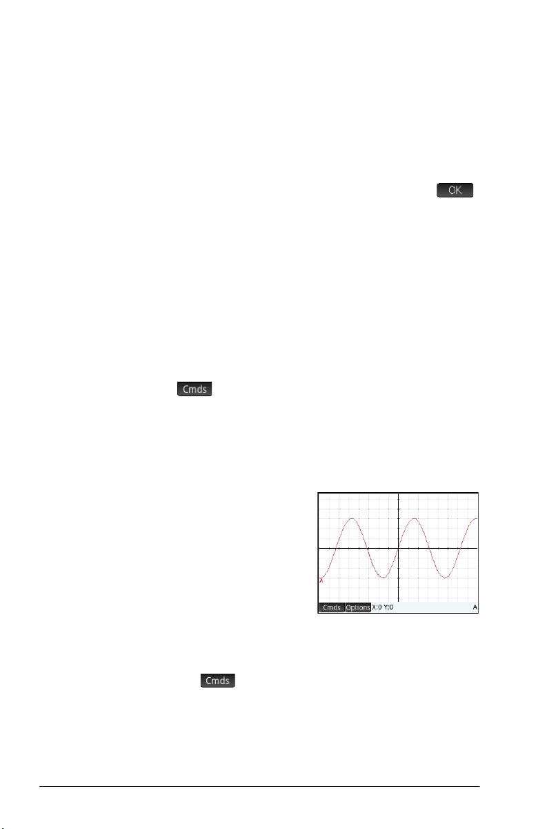
5. With plotfunc( on the entry line, enter 3*sin(x):

seASsE

Note that x must be entered in lowercase in the Geometry app.

If your graph doesn’t resemble the illustration at the right, adjust the

Rng

and Y Rng values in Plot Setup view (

SP).

We’ll now add a point to the curve, a point that will be constrained always to follow the contour of the curve.

Add a constrained point

6 Geometry

6. Tap , tap Point, and then select Point On.

Choosing Point On rather than Point means that the point will be constrained to whatever it is placed on.

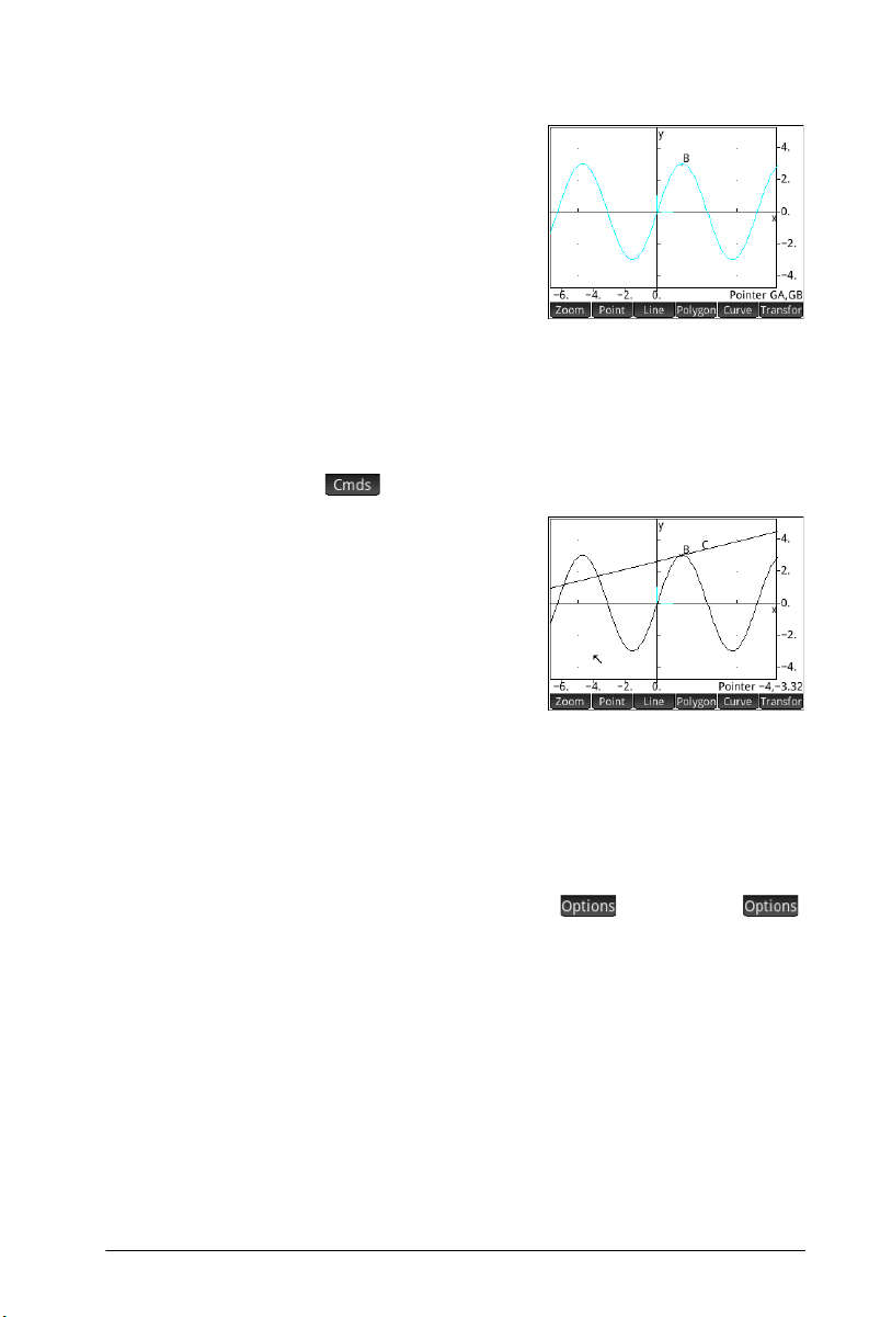
7. Ta p a ny wh ere on th e graph, press and then press

Notice that a point is added to the graph and given a name (B in this example). Tap a blank area of the screen to deselect everything. (Objects colored light blue are selected.)

Add a tangent 8. We will now add a tangent to the curve, making point B

the point of tangency:

> Line > Tangent

9. When prompted to select a curve, tap anywhere on the curve and press When prompted to select a point, tap point B and press see the tangent. Press

E to

J to close the Tangent tool.

Depending on where you placed point B, your illustration might be different from the one at the right. Now, make the tangent stand out by giving it a bright color.

10. Tap on the tangent to select it. After the tangent is selected, the new menu key appears. Tap or press Z, and then select Choose color.

11. Pick a color, and then tap on a blank area of the screen to see the new color of the tangent line.

12. Ta p p oin t B and drag it along the curve; the tangent moves accordingly. You can also drag the tangent line itself.

13. Ta p po in t B and then press The point turns light blue to show that it has been selected. Now, you can either drag the point with your finger or use the cursor keys for finer control of the

E to select the point.

Geometry 7

movement of point B. To deselect point B, either press J or tap point B and press

Note that whatever you do, point B remains constrained to the curve. Moreover, as you move point B, the tangent moves as well. If it moves off the screen, you can bring it back by dragging your finger across the screen in the appropriate direction.

Create a derivative point

The derivative of a graph at any point is the slope of its tangent at that point. We’ll now create a new point that will be constrained to point B and whose ordinate value is the derivative of the graph at point B. We’ll constrain it by forcing its x coordinate (that is, its abscissa) to always match that of point B, and its y coordinate (that is, its ordinate) to always equal the slope of the tangent at that point.

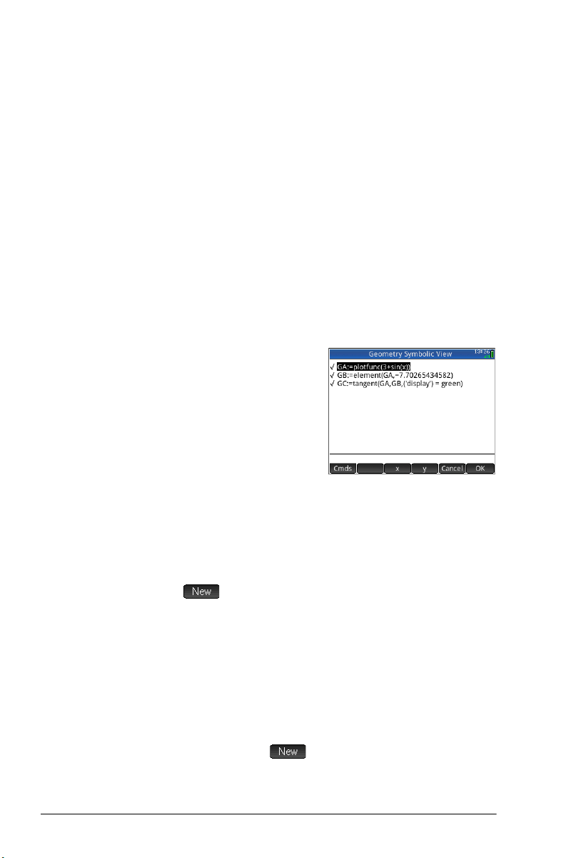
14. To define a point in terms of the attributes of other geometric objects, you need to go to Symbolic view:

Note that each object you have so far created is listed in Symbolic view. Note too that the name for an object in Symbolic view is the name it was given in Plot view but prefixed with a “G”. Thus the graph—labeled A in Plot view—is labeled GA in Symbolic view.

15. Highlight the blank definition following GC and tap

When creating objects that are dependent on other objects, the order in which they appear in Symbolic view is important. Objects are drawn in Plot view in the order in which they appear in Symbolic view. Since we are about to create a new point that is dependent on the attributes of GB and GC, it is important that we place its definition after that of both GB and GC. That is why we made sure we were at the bottom the list of definitions before tapping . If the new definition appeared higher up in Symbolic view, the point created in the following step would not be active in Plot view.

8 Geometry

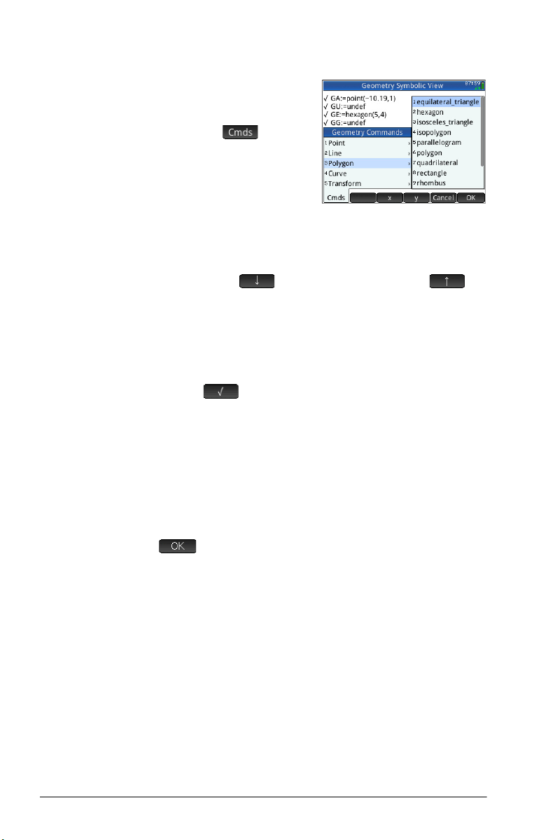
16. T a p a n d c h oos e Point > point

You now need to specify the x and y coordinates of the new point. The former is defined as the abscissa of point B (referred to as GB in Symbolic view) and the latter is defined as the slope of tangent line C (referred to as GC in Symbolic view).

17. Yo u sh o ul d ha v e point() on the entry line. Between the parentheses, add:

abscissa(GB),slope(GC)

For the abscissa command, tap , select Cartesian, and then select abscissa. For the slope command, tap

, select Measure, and then select slope.

18. Ta p .

The definition of your new point is added to Symbolic view. When you return to Plot view, you will see a point named D and it will have the same x- coordinate as point B.

19. Press

If you can’t see point D, pan until it comes into view. The y coordinate of D will be the derivative of the curve at point B.

Since it is difficult to read coordinates off the screen, we’ll add a calculation that will give the exact derivative (to three decimal places) and which we can display in Plot view.

Add some calculations

Geometry 9

20.Press M.

Numeric view is where you enter calculations.

21. Ta p .

22. Tap and choose Measure > slope

23. Between parentheses, add the name of the tangent, namely GC, and tap .

Notice that the current slope is calculated and displayed. The value here is dynamic, that is, if the slope of the tangent changes in Plot view, the value of the slope is automatically updated in Numeric view.

24.With the new calculation highlighted in Numeric view, tap .

Selecting a calculation in Numeric view means that it will also be displayed in Plot view.

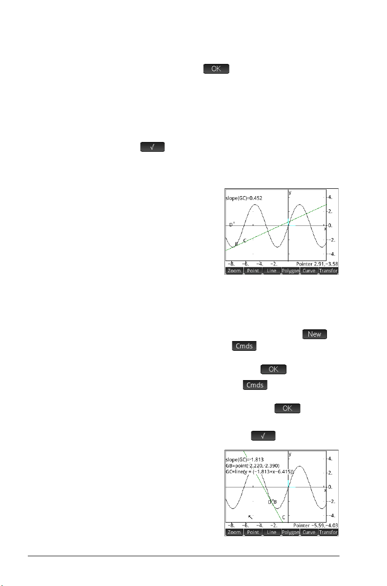
25. Press

26. Press

27. Tap the last blank field to select it, and then tap to

28.To start a third calculation, tap , select

29. Make sure both of these new equations are selected (by

30.Press

P to return to

Plot view.

Notice the calculation that you have just created in Numeric view is displayed at the top left of the screen.

Let’s now add two more calculations to Numeric view and have them displayed in Plot view.

M to return to Numeric view.

start a new calculation. Tap , select Cartesian, and then select Coordinates. Between the parentheses, enter GB and then tap .

Cartesian, and then select Equation of. Between the parentheses, enter GC and then tap .

choosing each one and pressing ).

P to return to

Plot view.

Notice that your new calculations are displayed.

10 Geometry

31. Ta p p oi n t B and then press E to select it.

32.Use the cursor keys to move point B along the graph. Note that with each move, the results of the calculations shown at the top left of the screen change. To deselect point B, tap point B and then press

Calculations in Plot view

Trace the derivative

By default, calculations in Plot view are docked to the upper left of the screen. You can drag a calculation from its dock and position it anywhere you like; however, after being undocked, the calculation scrolls with the display. Tap and hold a calculation to edit its label. An edit line opens so that you can enter your own label. You can also tap and select a different color for the calculation and its label. Tap when you are done.

Point D is the point whose ordinate value matches the derivative of the curve at point B. It is easier to see how the derivative changes by looking at a plot of it rather than comparing subsequent calculations. We can do that by tracing point D as it moves in response to movements of point B.

First we’ll hide the calculations so that we can better see the trace curve.

33. Press

34.Select each calculation in turn and tap . All

35. Press

36. Tap point D and then press E to select it.

37. Tap (or press Z) and then select Trace. Press

M to return to Numeric view.

calculations should now be deselected.

P to return to Plot view.

E to deselect point D.

38.Tap point B and then press

39. Using the cursor keys, move point B along the curve. Notice that a shadow curve is traced out as you move point B. This is the curve of the

E to select it.

Geometry 11

derivative of 3sin(x). Tap point B and then press E to deselect it.

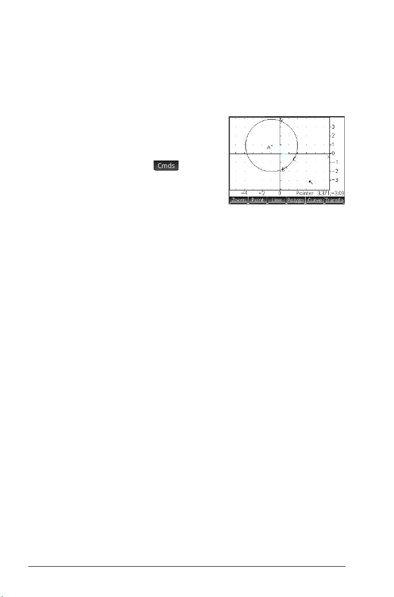
Plot view in detail

In Plot view you can directly draw objects on the screen using various drawing tools. For example, to draw a circle, tap , tap

Curve, and then select Circle. Now, tap where

you want the center of the circle to be and press on the circumference and press with a center at the location of your first tap, and with a radius equal to the distance between your first tap and second tap.

Note that there are on-screen instructions to help you. These instructions appear near the bottom of the screen, next to the command listing for the active tool (circle, point, and so on).

You can draw any number of geometric objects in Plot view. See “Plot view: Cmds menu” on page 23 for a list of the objects you can draw. The drawing tool you choose—line, circle, hexagon, and so on—remains selected until you deselect it. This enables you to quickly draw a number of objects of the same type (such as a number of hexagons). After you have finished drawing objects of a particular type, deselect the drawing tool by pressing drawing tool is still active by the presence of the on-screen instructions and the command name at the bottom of the screen.

An object in Plot view can be manipulated in numerous ways, and its mathematical properties can be easily determined (see page 20).

E. Next, tap a point that is to be

E. A circle is drawn

J. You can tell if a

Selecting objects Selecting an object involves at least two steps: tapping the

object and pressing to confirm your intention to select an object.

When you tap a location, objects recognized as being under the pointer are colored light red and added to the list of

12 Geometry

E. Pressing E is necessary

objects in the bottom right corner of the display. You can select any or all of these objects by pressing tap the screen and then use the cursor keys to accurately position the pointer before pressing

When more tha n one object is recognized as b eing under t he pointer, in most cases, preference is given to any point under the pointer when up box appears enabling you to select the desired objects.

You can also select multiple objects using a selection box. Tap and hold your finger at the location on the screen that represents one corner of the selection rectangle. Then drag your finger to the opposite corner of the selection rectangle. A light blue selection rectangle is drawn as you drag. Objects that touch this rectangle are selected.

E is pressed. In other cases, a pop-

E. You can

Hiding names You can choose to hide the name of an object in Plot view:

1. Select the object whose label you want to hide.

2. Tap or press

3. Select Hide Label.

Redisplay a hidden name by repeating this procedure and selecting Show Label.

Moving objects There are many ways to m ove objects. First, to move a n object

quickly, you can drag the object without selecting it.

Second, you can tap an object and press Then, you can drag the object to move it quickly or use the cursor keys to move it one pixel at a time. With the second method, you can select multiple objects to move together. When you have finished moving objects, tap a location where there are no objects and press If you have selected a single object, you can tap the object and press

Third, you can move a point on an object. Each point on an object has a calculation labeled with its name in Plot view. Tap and hold this item to display a slider bar. You can drag the slider or use the cursor keys to move it. appears as a new menu key. Tap this key to display a dialog box where you can specify the start, step, and stop values for the slider. Also, you can create an animation based on this point using

E to deselect it.

E to deselect everything.

E to select it.

Geometry 13

the slider. You can set the speed and pause for the animation, as well as its type. To start or stop an animation, select it, tap

, and then select or clear the Animate option.

Coloring objects Objects are colored black by default. The procedure to

change the color of an object depends on which view you are in. In both the Symbolic and Numeric view, each item includes a set of color icons. Tap these icons and select a color. In Plot view, select the object, tap (or press Z), tap Choose Color, and then select a color.

Filling objects An object with closed contours (such as a circle or polygon)

can be filled with color.

1. Se l e c t t h e o b je ct .

2. Tap or press Z.

3. Select Filled.

Filled is a toggle. To remove a fill, repeat the above procedure.

Clearing an object

14 Geometry

To clear one object, select it and tap C. Note that an object is distinct from the points you entered to create it. Thus deleting the object does not delete the points that define it. Those points remain in the app. For example, if you select a circle and press and radius point remain.

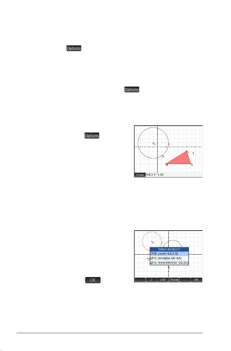
If other objects are dependent on the one you have selected for deletion, a pop-up displays the selected object and all dependent objects checked for deletion. Confirm your intention by tapping .

You can select multiple items for deletion. Either select them one at a time or use a selection box, and then press C.

Note that points you add to an object once the object has been defined are cleared when you clear the object. Thus if you place a point (say D) on a circle and delete the circle, the

C, the circle is deleted but the center point

circle and D are deleted, but the defining points—the center and radius points—remain.

Clearing all objects

Gestures in Plot view

To clear the app of all geometric objects, press SJ. You will be asked to confirm your intention to do so. Tap to clear all objects defined in Symbolic view or to keep the app as it is. You can clear all measurements and calculations in Numeric view in the same way.

You can pan by dragging a finger across the screen: either up, down, left, or right. You can also use the cursor keys to pan once the cursor is at the edge of the screen. You can use a pinch gesture to zoom in or out. Place two fingers on the screen. Move them apart to zoom in or bring them together to zoom out. You can also press + to zoom in on the pointer or press w to zoom out on the pointer.

Zooming You can zoom by tapping and choosing a zoom

option. The zoom options are the same as you find in the Plot view of many apps in the calculator.

Geometry 15

Plot view: buttons and keys

Button or key Purpose

Opens the Commands menu. See “Plot view: Cmds menu” on page 23.

Opens the Options menu for the selected object.

Hides (or displays) the axes.

J SJ

Selects the circle drawing tool. Follow the instructions on the screen (or see page

28). Erases all trace lines.

Selects the intersection drawing tool. Follow the instructions on the screen (or see page 24).

Selects the line drawing tool. Follow the instructions on the screen (or see page

25). Selects the point drawing tool. Follow the

instructions on the screen (or see page

24) . Selects the segment drawing tool. Follow

the instructions on the screen (or see page

25). Selects the triangle drawing tool. Follow

the instructions on the screen (or see page

26) . Deletes a selected object (or the character

to the left of the cursor if the entry line is active).

Deselects the current drawing tool.

Clears the Plot view of all geometric objects or the Numeric view of all measurements and calculations.

16 Geometry

The Options menu

When you select an object, a new menu key appears:

object, such as color. The Options menu changes depending on the type of object selected. The complete set of Geometry options are listed in the following table and are also displayed when you press Z.

. Tap this key to view and select options for the selected

Option

Choose Color

Hide

Hide Label

Filled

Trace

Clear Trace

Animate

Purpose

Displays a set of color icons so you can select a color for the selected object.

Hides the selected object. This is a shortcut for deselecting the object in Symbolic view. To select an object to display after it has been hidden, go to Symbolic or Numeric view.

Hides the label of a selected object. This option changes to Show Label if the selected object has a hidden label.

Fills the selected object with a color. Clear this option to remove the fill.

Starts tracing for any selected point if selected, then stops tracing for the selected point.

Erases the current trace of the selected point but does not stop tracing.

Starts the current animation of a selected point on an object. If the selected point is currently animated, this option stops the animation.

Geometry 17

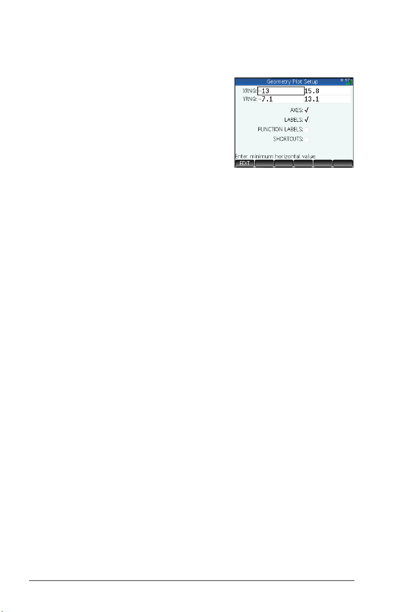
Plot Setup view

The Plot Setup view enables you to configure the appearance of Plot view.

The fields and options are as follows:

•

X Rng: There are two

boxes, but only the minimum x-value is editable. The maximum x-value is calculated automatically, based on the minimum value and the pixel size. You can also change the x range by panning and zooming in Plot view.

•

Y Rng: There are two boxes, but only the minimum y-

value is editable. The maximum y-value is calculated automatically, based on the minimum value and the pixel size. You can also change the y range by panning and zooming in Plot view.

• Pixel Size: Each pixel in the Plot view must be square.

You can change the size of each pixel. The lower left corner of the Plot view display remains the same, but the upper right-corner coordinates are automatically recalculated.

•

Axes: A toggle option to hide (or show) the axes in Plot

view.

Keyboard shortcut:

• Labels: A toggle option to hide (or show) the labels for the axes.

•

Grid Dots: A toggle option to hide (or show) the grid

dots.

• Grid Lines: A toggle option to hide (or show) the grid lines.

18 Geometry

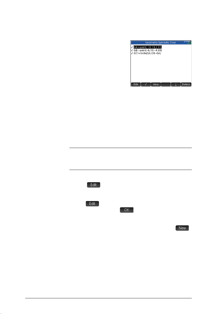
Symbolic view in detail

Every object—whether a point, segment, line, polygon, or curve—is given a name, and its definition is displayed in Symbolic view (

Y). The name is the

name for it you see in Plot view, but prefixed by “G”. Thus a point labeled A in Plot view is given the name GA in Symbolic view.

The G-prefixed name is a variable that can be read by the computer algebra system (CAS). Thus in the CAS you can include such variables in calculations. Note in the illustration above that GC is the name of the variable that represents a circle drawn in Plot view. If you are working in the CAS and wa nted to know what the are a of that ci rcle is, you c ould enter area(GC) and press

Note

Calculations referencing geometry variables can be made in the CAS or in the Numeric view of the Geometry app (explained below on page 20).

You can change the definition of an object by selecting it, tapping , and altering one or more of its defining parameters. The object is modified accordingly in Plot view. For example, if you selected point GB in the illustration above, tapped , changed one or both of the point’s coordinates, and tapped , you would find, on returning to Plot view, a circle of a different size.

Creating objects You can also create an object in Symbolic view. Tap ,

define the object—for example, point(4,6)—and press

E. The object is created and can be seen in Plot view.

Another example: to draw a line through points P and Q, enter line(GP,GQ) in Symbolic view and press When you return to Plot view, you will see a line passing through points P and Q.

Geometry 19

The object-creation commands available in Symbolic view can be seen by tapping . The syntax for each command is given in “Geometry functions and commands” on page 39.

Re-ordering entries

You can re-order the entries in Symbolic view. Objects are drawn in Plot view in the order in which they are defined in Symbolic view. To change the position of an entry, highlight it and tap either (to move it down the list) or (to move it up).

Hiding an object To prevent an object displaying in Plot view, deselect it in

Symbolic view:

1. Highlight the item to be hidden.

2. Tap .

Repeat the procedure to make the object visible again.

Deleting an object

As well as deleting an object in Plot view (see page 14) you can delete an object in Symbolic view.

1. Highlight the definition of the object you want to delete.

2. Press

To delete all objects, press

SJ. When prompted, tap

to confirm the deletion.

Symbolic Setup view

The Symbolic view of the Geometry app is common with many apps. It is used to override certain system-wide settings.

Numeric view in detail

Numeric view (M) enables you to do calculations in the Geometry app. The results displayed are dynamic—if you manipulate an object in Plot view or Symbolic view, any calculations in Numeric view that refer to that object are

20 Geometry

automatically updated to reflect the new properties of that object.

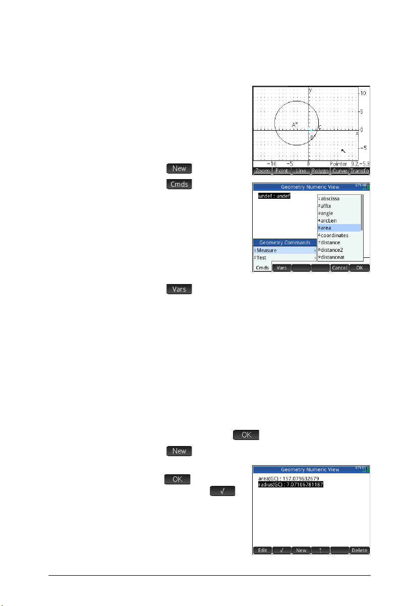
Consider circle C in the illustration at the right. To calculate the area and radius of C:

1. Press

2. Tap .

3. Tap and choose

4. Tap , choose Curves and then the curve whose

5. Press

6. Tap .

7. E n t e r radius(GC) and

M to open

Numeric view.

Measure > Area.

Note that area() appears on the entry line, ready for you to specify the object whose area you are interested in.

area you are interested in.

The name of the object is placed between the parentheses.

You could have entered the command and object name manually, that is, without choosing them from menus. If you enter object names manually, remember that the name of the object in Plot view must be given a “G” prefix if it is used in any calculation. Thus the circle named C in Plot view must be referred to as GC in Numeric view and Symbolic view.

E or tap . The area is displayed.

tap . The radius is displayed. Use to verify both of these measurements so that they will be available in Plot view.

Geometry 21

Note

Note that the syntax used here is the same as you use in the CAS to calculate the properties of geometric objects.

The Geometry functions and their syntax are described in “Geometry functions and commands” on page 39.

8. Press

If an entry in Numeric view is too long for the screen, you can press > to scroll the rest of the entry into view. Press < to scroll back to the original view.

P to go back to Plot view. Now, manipulate the

circle in some way that changes its area and radius. For example, select the center point (A) and use the cursor keys to move it to a new location. Notice that the area and radius calculations update automatically as you move the point. Remember to press J finished.

when you are

Listing all objects

Displaying calculations in Plot view

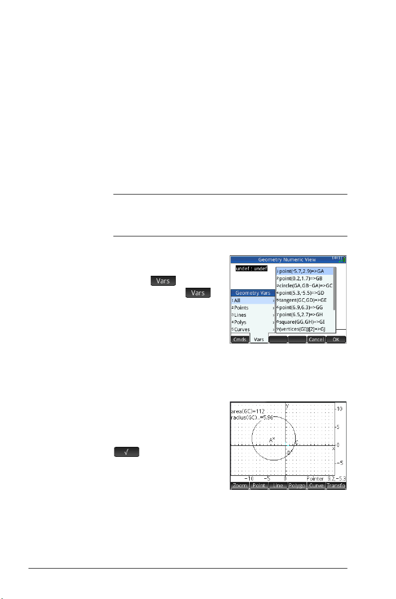
When you are creating a new calculation in Numeric view, the menu item appears. Tapping gives you a list of all the objects in your Geometry workspace.

If you are building a calculation, you can select an object’s vari able na me from this menu. The name of the selected object is placed at the insertion point on the entry line.

To have a calculation made in Numeric view appear in Plot view, just highlight it in Numeric view and tap

. A checkmark appears beside the calculation.

Repeat the procedure to prevent the calculation being displayed in Plot view. The checkmark is cleared.

22 Geometry

Editing a calculation

1. Highlight the calculation that you want to edit.

2. Tap to change the calculation or tap to change the label.

3. Make your changes and tap .

Deleting a calculation

1. Highlight the calculation you want to delete.

2. Press C.

To delete all calculations, press a calculation does not delete any geometric objects from either the Plot or Symbolic view.

Plot view: Cmds menu

The geometric objects discussed in this section are those that can be created in either Plot view or Symbolic view using the Commands menu ( ). This section discusses how to use the commands in Plot view. Objects can also be created in Symbolic view—more, in fact, than in Plot view—but these are discussed in “Geometry functions and commands” on page 39. Finally, measurements and other calculations can be performed in Plot view as well.

In Plot view, you ch oose a drawing tool to draw an object. The tools are listed in this section. Note that once you select a drawing tool, it remains selected until you deselect it. This enables you to quickly draw a number of objects of the same type (such as a number of circles). To deselect the current drawing tool, press active by the presence of the on-screen help in the bottom leftside of the screen and the current command statement to its right.

The steps provided in this section are based on touch entry. For example, to add a point, the steps will tell you to tap on the screen where you want the point to be and press However, you can also use the cursor keys to position the cursor where you want the point to be and then press

The drawing tools for the geometric objects listed in this section can be selected from the Commands menu at the bottom of the screen ( ). Some objects can also be

SJ. Note that deleting

J. You can tell if a drawing tool is still

Geometry 23

entered using a keyboard shortcut. For example, you can select the triangle drawing tool by pressing view: buttons and keys” on page 16.

n. See “Plot

Point Tap to display a menu and submenus of options for

entering various types of points. The menus and submenus are:

Point Tap where you want the point to be and press

Keyboard shortcut: B

Point On Tap the object where you want the new point to be and press

E. If you select a point that has been placed on an

object and then move that point, the point will be constrained to the object on which it was placed. For example, a point placed on a circle will remain on that circle regardless of how you move the point.

Midpoint Tap where you want one point to be and press

where you want the other point to be and press point is automatically created midway between those two points.

If you choose an object first—such as a segment—choosing the Midpoint tool and pressing between the ends of that object. (In the case of a circle, the midpoint is created at the circle’s center.)

Center Tap a circle and press

center of the circle.

Intersection Tap the desired intersection and press E. A point is

created at one of the points of intersection.

Keyboard shortcut:

E. A point is created at the

E adds a point midway

E. Tap

E. A

Intersections Tap one object other than a point and press E. Tap

another object and press objects intersect are created and named. Note that an intersections object is created in Symbolic view even if the two objects selected do not intersect.

24 Geometry

E. The point(s) where the two

Random Points Press E to randomly create a point in Plot view.

Continue pressing E to create more random points. Press J when you are done.

Line

Segment Tap where you want one endpoint to be and press E.

Tap where you want the other endpoint to be and press

E. A segment is drawn between the two end points.

Keyboard shortcut: r

Ray Tap where you want the endpoint to be and press E.

Tap a point that you want the ray to pass through and press

E. A ray is drawn from the first point and through the

second point.

Line Tap at a point you want the line to pass through and press

E. Tap at another point you want the line to pass

through and press points.

Keyboard shortcut: Tap a third point (C) and press E. A line is drawn

through A bisecting the angle formed by AB

E. A line is drawn through the two

and AC.

Parallel Tap on a point (P) and press

press

E. A new line is draw parallel to L and passing

through P.

Perpendicular Tap on a point (P) and press E. Tap on a line (L) and

press

E. A new line is draw perpendicular to L and

passing through P.

Tangent Tap on a curve (C) and press E. Tap on a point (P) and

press

E. If the point (P) is on the curve (C), then a single

tangent is drawn. If the point (P) is not on the curve (C), then zero or more tangents may be drawn.

Median Tap on a point (A) and press

E. A line is drawn through the point (A) and the

press midpoint of the segment.

Geometry 25

E. Tap on a line (L) and

E. Tap on a segment and

Altitude Tap on a point (A) and press E. Tap on a segment and

press

E. A line is drawn through the point (A)

perpendicular to the segment (or its extension).

Angle bisector Tap the point that is the vertex of the angle to be bisected (A)

and press

E. Tap another point (B) and press E.

Polygon The Polygon menu provides tools for drawing various

polygons.

Triangle Tap at each vertex, pressing E after each tap.

Keyboard shortcut: n

Isosceles Triangle

Right Triangle Draws a right triangle given two points and a scale factor.

Draws an isosceles triangle defined by two of its vertices and an angle. The vertices define one of the two sides equal in length and the angle defines the angle between the two sides of equal length. Like equilateral_triangle, you have the option of storing the coordinates of the third point into a CAS variable.

isosceles_triangle(point1, point2, angle)

Example:

isosceles_triangle(GA, GB, angle(GC, GA, GB) defines an isosceles triangle such that one of the two sides of equal length is AB, and the angle between the two sides of equal length has a measure equal to that of ∡ ACB.

One leg of the right triangle is defined by the two points, the vertex of the right angle is at the first point, and the scale factor multiplies the length of the first leg to determine the length of the second leg.

right_triangle(point1, point2, realk)

Example:

right_triangle(GA, GB, 1) draws an isosceles right triangles with its right angle at point A, and with both legs equal in length to segment AB.

Quadrilateral Tap at each vertex, pressing

26 Geometry

E after each tap.

Parallelogram Tap at one vertex and press E. Tap at another vertex

and press

E. Tap at a third vertex and press E.

The location of the fourth vertex is automatically calculated and the parallelogram is drawn.

Rhombus Draws a rhombus, given two points and an angle. As with

many of the other polygon commands, you can specify optional CAS variable names for storing the coordinates of the other two vertices as points.

rhombus(point1, point2, angle)

Example

rhombus(GA, GB, angle(GC, GD, GE)) draws a rhombus on segment AB such that the angle at vertex A has the same measure as ∡ DCE.

Rectangle Draws a rectangle given two consecutive vertices and a point

on the side opposite the side defined by the first two vertices or a scale factor for the sides perpendicular to the first side. As with many of the other polygon commands, you can specify optional CAS variable names for storing the coordinates of the other two vertices as points.

rectangle(point1, point2, point3) or rectangle(point1, point2, realk)

Examples:

rectangle(GA, GB, GE) draws a rectangle whose first two vertices are points A and B (one side is segment AB). Point E is on the line that contains the side of the rectangle opposite segment AB.

rectangle(GA, GB, 3, p, q) draws a rectangle whose first two vertices are points A and B (one side is segment AB). The sides perpendicular to segment AB have length 3*AB. The third and fourth points are stored into the CAS variables p and q, respectively.

Polygon Draws a polygon from a set of vertices.

polygon(point1, point2, …, pointn)

Example: polygon(GA, GB, GD) draws ΔABD

Geometry 27

Regular Polygon

Square Tap at one vertex and press E. Tap at another vertex

Draws a regular polygon given the first two vertices and the number of sides, where the number of sides is greater than 1. If the number of sides is 2, then the segment is drawn. You can provide CAS variable names for storing the coordinates of the calculated points in the order they were created. The orientation of the polygon is counterclockwise.

isopolygon(point1, point2, realn), where realn is an integer greater than 1.

Example

isopolygon(GA, GB, 6) draws a regular hexagon whose first two vertices are the points A and B.

and press vertices are automatically calculated and the square is drawn.

E. The location of the third and fourth

Curve

Circle Tap at the center of the circle and press E. Tap at a

point on the circumference and press drawn about the center point with a radius equal to the distance between the two tapped points.

Keyboard shortcut:

You can also create a circle by first defining it in Symbolic view. The syntax is circle(GA,GB) where A and B are two points. A circle is drawn in Plot view such that A and B define the diameter of the circle.

E. A circle is

Circumcircle A circumcircle is the circle

that passes through each of the triangle’s three vertices, thus enclosing the triangle.

Tap at each vertex of the triangle, pressing after each tap.

Excircle An excircle is a circle that is tangent to one segment of a

triangle and also tangent to the rays through the segment’s endpoints from the vertex of the triangle opposite the segment.

28 Geometry

Tap at each vertex of the triangle, pressing after each tap.

The excircle is drawn tangent to the side defined by the last two vertices tapped. In the example at the right, the last two vertices tapped were A and C (or C and A). Thus the excircle is drawn tangent to the segment AC

Incircle An incircle is a circle that is tangent to all three sides of a

triangle. Tap each vertex of the triangle, pressing E after each tap.

Ellipse Tap at one focus point and press E. Tap at the second

focus point and press circumference and press

E. Tap at point on the

Hyperbola Tap at one focus point and press

focus point and press the hyperbola and press

Parabola Tap at the focus point and press

(the directrix) or a ray or segment nd press

Conic Plots the graph of a conic section defined by an expression in

x and y.

conic(expr)

Example:

conic(x^2+y^2-81) draws a circle with center at (0,0) and radius of 9

Locus Takes two points as its arguments: the first is the point whose

possible locations form the locus; the second is a point on an object. This second point drives the first through its locus as the second moves on its object.

Geometry 29

E. Tap at point on one branch of

E. Tap at the second

E. Tap either on a line

In the example at the right, circle C has been drawn and point D is a point placed on C (using the Point On function described above). Point I is a translation of point D. Choosing Curve >

Special > Locus places locus( on the entry line. Complete the command as locus(GI,GD) and point I traces a path (its locus) that

parallels point D as it moves around the circle to which it is constrained.

Plot You can plot expressions of the following types in Plot view:

• Function

• Parametric

• Polar

• Sequence

Tap , select then the type of expression you want to plot. The entry line is enabled for you to define the expression.

Note that the variables you specify for an expression must be in lowercase.

In this example, has been selected as the plot type and the graph of y = 1/ x is plotted.

Plot, and

Function

Function Syntax: plotfunc(Expr)

Draws the plot of a function, given an expression in the independent variable x. An edit line appears. Enter your expression and press E. Note the use of lowercase x.

30 Geometry

Example:

plotfunc(3*sin(x)) draws the graph of y=3*sin(x)

Parametric Syntax: plotparam(f(Var)+i*g(Var), Var=

Start..Stop, [tstep=Value])

Takes a complex expression in one variable and an interval for that variable as arguments. Interprets the complex expression f(t)+i*g(t) as x=f(t) and y=g(t) and plots the parametric equation over the interval specified in the second argument. An edit line opens for you to enter the complex expression and the interval.

Examples:

plotparam(cos(t)+ i*sin(t), t=0..2*π) plots the unit circle

plotparam(cos(t)+ i*sin(t), t=0..2*π, tstep=π/3) plots a regular hexagon inscribed in the unit

circle (note the tstep value)

Polar Syntax: plotpolar(Expr,Var=Interval, [Step]) or

plotpolar(Expr, Var, Min, Max, [Step])

Draws a polar graph in Plot view. An edit line opens for you to enter an expression in x as well as an interval (and optional step).

plotpolar(f(x),x,a,b) draws the polar curve r=f(x) for x in [a,b]

Sequence Syntax: plotseq(f(Var), Var={Start, Xmin,

Xmax}, Integer n)

Given an expression in x and a list containing three values, draws the line y=x, the plot of the function defined by the expression over the domain defined by the interval between the last two values, and draws the cobweb plot for the first n terms of the sequence defined recursively by the expression (starting at the first value).

Geometry 31

Example:

plotseq(1-x/2, x={3 -1 6}, 5) plots y=x and y=1–x/2 (from x=–1 to x=6), then draws the first 5 terms of the cobweb plot for u(n)=1-(u(n–1)/2, starting at u(0)=3

Implicit Syntax: plotimplicit(Expr, [XIntrvl, YIntrvl])

Plots an implicitly defined curve from Expr (in x and y). Specifically, plots Expr=0. Note the use of lowercase x and y. With the optional x-interval and y-interval, this command plots only within those intervals.

Example:

plotimplicit((x+5)^2+(y+4)^2-1) plots a circle, centered at the point (-5, -4), with a radius of 1

Slopefield Syntax: plotfield(Expr, [x=X1..X2 y=Y1..Y2],

[Xstep, Ystep], [Option])

Plots the graph of the slopefield for the differential equation y’=f(x,y) over the given x-range and y-range. If Option is normalize, the slopefield segments drawn are equal in length.

Example:

plotfield(x*sin(y), [x=-6..6, y=-

6..6],normalize) draws the slopefield for y'=x*sin(y), from -6 to 6 in both directions, with

segments that are all of the same length

ODE Syntax: plotode(Expr, [Var1, Var2, ...],

[Val1, Val2. ...])

Draws the solution of the differential equation y’=f(Var1, Var2, ...) that contains as initial condition for the variables Val1, Val2,... The first argument is the expression f(Var1, Var2,...), the second argument is the vector of variables, and the third argument is the vector of initial conditions.

Example:

plotode(x*sin(y), [x,y], [–2, 2]) draws the graph of the solution to y’=x*sin(y) that passes through the point (–2, 2) as its initial condition

32 Geometry

List Syntax: plotlist(Matrix 2xn)

Plots a set of n points and connects them with segments. The points are defined by a 2xn matrix, with the abscissas in the first row and the ordinates in the second row.

Example:

plotlist([[0,3],[2,1],[4,4],[0,3]]) draws a triangle

Slider Creates a slider bar that can be used to control the value of

a parameter. A dialog box displays the slider bar definition and any animation for the slider.

Transform The Transform menu provides numerous tools for you to

perform transformations on geometric objects in Plot view. You can also define transformations in Symbolic view

Translation A translation is a transformation of a set of points that moves

each point the same distance in the same direction. T: (x,y) → (x+a, y+b).

Suppose you want to translate circle B at the right down a little and to the right:

1. Tap , tap

Transform, and select Translation.

2. Tap the object to be moved and press

3. Tap an initial location and press

4. Tap a final location and press

The object is moved the same distance and direction from the initial to the final locations. The original object is left in place.

Geometry 33

Reflection A reflection is a

transformation which maps an object or set of points onto its mirror image, where the mirror is either a point or a line. A reflection through a point is sometimes called a half-turn. In either case, each point on the mirror image is the same distance from the mirror as the corresponding point on the original. In the example at the right, the original triangle D is reflected through point I.

1. Tap , tap Transform, and select Reflection.

2. Tap the point or straight object (segment, ray, or line) that will be the symmetry axis (that is, the mirror) and press

3. Tap the object that is to be reflected across the symmetry axis and press symmetry axis defined in step 2.

Rotation A rotation is a mapping that

rotates each point by a fixed angle around a center point. The angle is defined using the angle() command, with the vertex of the angle as the first argument. Suppose you wish to rotate the square (GC) around point K (GK) through figure to the right.

1. Tap , tap Transform, and select Rotation.

rotation() appears on the entry line.

2. Between the parentheses, enter:

GK,angle(GK,GL,GM ),GC

3. Press

E or tap

E. The object is reflected across the

∡ LKM in the

34 Geometry

4. Press P to return to Plot view to see the rotated square.

Dilation A dilation (also called a homothety or uniform scaling) is a

transformation where an object is enlarged or reduced by a given scale factor around a given point as center.

In the illustration at the right, the scale factor is 2 and the center of dilation is indicated by a point near the top right of the screen (named I). Each point on the new triangle is collinear with its corresponding point on the original triangle and point I. Further, the distance from point I to each new point will be twice the distance to the original point (since the scale factor is 2).

1. Tap , tap Transform, and select Dilation.

2. Tap the point that is to be the center of dilation and press

3. Enter the scale factor and press E.

4. Tap the object that is to be dilated and press

Similarity Dilates and rotates a geometric object about the same center

point.

similarity(point, realk, angle, object)

Example:

similarity(0, 3, angle(0,1,i),point(2,0))

dilates the point at (2,0) by a scale factor of 3 (a point at (6,0)), then rotates the result 90° counterclockwise to create a point at (0, 6).

Projection A projection is a mapping of one or more points onto an

object such that the line passing through the point and its image is perpendicular to the object at the image point.

1. Tap , tap Transform, and select Projection.

2. Tap the object onto which points are to be projected and press

Geometry 35

3. Tap the point that is to be projected and press E.

Note the new point added to the target object.

Inversion An inversion is a mapping involving a center point and a

scale factor. Specifically, the inversion of point A through center C, with scale factor k, maps A onto A’, such that A’ is on line CA and CA*CA’=k, where CA and CA’ denote the lengths of the corresponding segments. If k=1, then the lengths CA and CA’ are reciprocals.

Suppose you wish to find the inversion of point B with respect to point A.

1. Tap , tap Transform, and select Inversion.

2. Tap point A and press

3. Enter the inversion ratio—use the default value of 1—and press

4. Tap point B and press

In the figure, point C is the inversion of point B in respect to point A.

Reciprocation A reciprocation is a special case of inversion involving circles.

A reciprocation with respect to a circle transforms each point in the plane into its polar line. Conversely, the reciprocation with respect to a circle maps each line in the plane into its pole.

1. Tap , tap Transform, and select Reciprocation.

2. Tap the circle and press

36 Geometry

3. Tap a point and press

E to see its polar

line.

4. Tap a line and press

E to see its pole.

In the illustration to the right, point K is the reciprocation of line DE (G) and Line I (at the bottom of the display) is the reciprocation of point H.

Cartesian

Abcissa Tap a point and press E to select it. The abscissa (x-

coordinate) of the point will appear at the top left of the screen.

Ordinate Tap a point and press E to select it. The ordinate (y-

coordinate) of the point will appear at the top left of the screen.

Coordinates Tap a point and press E to select it. The coordinates of

the point will appear at the top left of the screen.

Equation of Tap an object other than a point and press E to select

it. The equation of the object (in x and/or y) is displayed.

Parametric Tap an object other than a point and press E to select

it. The parametric equation of the object (x(t)+i*y(t)) is displayed.

Polar coordinates

Tap a point and press E to select it. The polar coordinates of the point will appear at the top left of the screen.

Measure

Distance Tap a point and press E to select it. Repeat to select a

second point. The distance between the two points is displayed.

Geometry 37

Radius Tap a circle and press E to select it. The radius of the

circle is displayed.

Perimeter Tap a circle and press E to select it. The perimeter of the

circle is displayed.

Slope Tap a straight object (segment, line, and so on) and press

E to select it. The slope of the object is displayed.

Area Tap a circle or polygon and press E to select it. The area

of the object is displayed.

Angle Tap a point and press E to select it. Repeat to select

three points. The measure of the directed angle from the second point through the third point, with the first point as vertex, is displayed.

Arc Length Tap a curve and press E to select it. Then, enter a start

value and a stop value. The length of the arc on the curve between the two x-values is displayed.

Tests

Collinear Tap a point and press E to select it. Repeat to select

three points. The test appears at the top of the display, along with its result. The test returns 1 if the points are collinear; otherwise, it returns 0.

On circle Tap a point and press E to selec t it. Repeat to select four

points. The test appears at the top of the display, along with its result. The test returns 1 if the points are on the same circle; otherwise, it returns 0.

On object Tap a point and press E to select it. Then tap an object

and press E. The test appears at the top of the display, along with its result. The test returns 1 if the point is on the object; otherwise, it returns 0.

Parallel Tap a straight object (segment, line, and so on) and press

E to select it. Then tap another straight object and press E. The test appears at the top of the display, along with

38 Geometry

its result. The test returns 1 if the objects are parallel; otherwise, it returns 0.

Perpendicular Tap a straight object (segment, line, and so on) and press

E to select it. Then tap another straight object and press E. The test appears at the top of the display, along with

its result. The test returns 1 if the objects are perpendicular; otherwise, it returns 0.

Isosceles Tap a triangle and press E to select it. Or select three

points in order. Returns 0 if the triangle is not isosceles or if the three points do not form an isosceles triangle. If the triangle is isosceles (or the three points form an isosceles triangle), returns the number order of the common point of the two sides of equal length (1, 2, or 3). Returns 4 if the three points form an equilateral triangle or if the selected triangle is equilateral.

Equilateral Tap a triangle and press E to select it. Or select three

points in order. Returns 1 if the triangle is equilateral or if the three points form an equilateral triangle; otherwise, it returns

Parallelogram Tap a point and press E to select i t. Repeat to se lect four

points. The test appears at the top of the display, along with its result. The test returns 0 if the points do not form a parallelogram. Returns 1 if they form a parallelogram, 2 if they form a rhombus, 3 if they form a rectangle, and 4 if they form a square.

Conjugate Tap a circle and press E to select it. Then, select two

points or two lines. The test returns 1 if the two points or lines are conjugates for the circle; otherwise, it returns 0.

Geometry functions and commands

The list of geometry-specific functions and commands in this section covers those that can be found by tapping in both Symbolic and Numeric view and those that are only available from the Catlg menu.

Geometry 39

The sample syntax provided has been simplified. Geometric objects are referred to by a single uppercase character (such as A, B,C and so on). However, calculations referring to geometric objects—in the Numeric view of the Geometry app and in the CAS—must use the G-prefixed name given for it in Symbolic view. For example:

altitude(A,B,C) is the simplified form given in this section

altitude(GA,GB,GC) is the form you need to use in calculations

Further, in many cases the specified parameters in the syntax below—A, B, C etc.—can be the name of a point (such as GA) or a complex number representing a point. Thus angle(A,B,C) could be:

• angle(GP,GR, GB)

• angle(3+2i,1–2i, 5+i) or

• a combination of named points and points defined by a

complex number, as in angle(GP,1–2*i,i).

Symbolic view: Cmds menu

For the most part, the Commands menu in Symbolic View is the same as it is in Plot view. The Zoom category does not appear in Symbolic view, nor do the Cartesian, Measure, and Tests categories, although the latter three appear in Numeric view. In Symbolic view, the commands are entered using their syntax. Highlight a command and press W to learn its syntax. The advantage of entering or editing a definition in Symbolic view is that you can specify the exact location of points. After the exact locations of points are entered, the properties of any dependent objects (lines, circles, and so on) are reported exactly by the CAS. Use this fact to test conjectures on geometric objects using the Test commands. All these commands can be used in the CAS view, where they return the same objects.

40 Geometry

Point

Point on

Midpoint

Creates a point, given the coordinates of the point. Each coordinate may be a value or an expression involving variables or measurements on other objects in the geometric construction.

point(real1, real2) or point(expr1, expr2)

Examples:

point(3,4) creates a point whose coordinates are (3,4). This point may be selected and moved later.

point(abscissa(A), ordinate(B)) creates a point whose x-coordinate is the same as that of a point A and whose y-coordinate is the same as that of a point B. This point will change to reflect the movements of point A or point B.

Creates a point on a geometric object whose abscissa is a given value or creates a real value on a given interval.

element(object, real) or element(real1..real2)

Examples:

element(plotfunc(x

graph of y = x

. Initially, this point will appear at (–2,4). You

),–2) creates a point on the

can move the point, but it will always remain on the graph of its function.

element(0..5) creates a slider bar with a value of 2.5 initially. Tap and hold this value to open the slider. Select or

< to increase or decrease the value on the slider bar.

Press J to close the slider bar. The value that you set can be used as a coefficient in a function that you subsequently plot or in some other object or calculation.

Returns the midpoint of a segment. The argument can be either the name of a segment or two points that define a segment. In the latter case, the segment need not actually be drawn.

midpoint(segment) or midpoint(point1, point2)

Example: midpoint(0,6+6i) returns point(3,3)

Geometry 41

Center

Intersection

Intersections

Line

Segment

Syntax: center(Circle)

Plots the center of a circle. The circle can be defined by the circle command or by name (for example, GC).

Example: center(circle(x^2+y2–x–y)) plots

point(1/2,1/2)

Syntax: single_inter(Curve1, Curve2, [Point])

Plots the intersection of Curve1 and Curve2 that is closest to Poi nt.

Example:

single_inter(line(y=x), circle(x^2+y^2=1), point(1,1)) plots point((1+i)*√2/2)

Returns the intersection of two curves as a vector.

inter(Curve1, Curve2)

Example:

inter(8-x^2/6, x/2-1)

returns

[[6 2],[-9 -11/2]]

Draws a segment defined by its endpoints.

segment(point1, point2)

Examples:

segment(1+2i, 4) draws the segment defined by the points whose coordinates are (1, 2) and (4, 0).

segment(GA, GB) draws segment AB.

Ray

Given 2 points, draws a ray from the first point through the second point.

half_line((point1, point2)

42 Geometry

Line

Parallel

Perpendicular

Draws a line. The arguments can be two points, a linear expression of the form a*x+b*y+c, or a point and a slope as shown in the examples.

line(point1, point2) or line(a*x+b*y+c) or line(point1, slope=realm)

Examples:

line(2+i, 3+2i) draws the line whose equation is y=x–1; that is, the line through the points (2,1) and (3,2).

line(2x–3y–8) draws the line whose equation is 2x–3y=8

line(3–2i,slope=1/2) draws the line whose equation is x–2y=7; that is, the line through (3, –2) with slope m=1/2.

Draws a line through a given point that is parallel to a given line.

parallel(point,line)

Examples:

parallel(A, B) draws the line through point A that is parallel to line B.

parallel(3–2i, x+y–5) draws the line through the point (3, –2) that is parallel to the line whose equation is x+y=5; that is, the line whose equation is y=–x+1.

Draws a line through a given point that is perpendicular to a given line. The line may be defined by its name, two points, or an expression in x and y.

perpendicular(point, line) or perpendicular(point1, point2, point3)

Examples:

perpendicular(GA, GD) draws a line perpendicular to line D through point A.

perpendicular(3+2i, GB, GC) draws a line through the point whose coordinates are (3, 2) that is perpendicular to line BC.

Geometry 43

Tangent

Median

Altitude

perpendicular(3+2i,line(x–y=1)) draws a line through the point whose coordinates are (3, 2) that is perpendicular to the line whose equation is x – y = 1; that is, the line whose equation is y=–x+5.

Draws the tangent(s) to a given curve through a given point. The point does not have to be a point on the curve.

tangent(curve, point)

Examples:

tangent(plotfunc(x^2), GA) draws the tangent to the graph of y=x^2 through point A.

tangent(circle(GB, GC–GB), GA) draws one or more tangent lines through point A to the circle whose center is at point B and whose radius is defined by segment BC.

Given three points that define a triangle, creates the median of the triangle that passes through the first point and contains the midpoint of the segment defined by the other two points.

median_line(point1, point2, point3)

Example:

median_line(0, 8i, 4) draws the line whose equation is y=2x; that is, the line through (0,0) and (2,4), the midpoint of the segment whose endpoints are (0, 8) and (4, 0).

Given three non-collinear points, draws the altitude of the triangle defined by the three points that passes through the first point. The triangle does not have to be drawn.

altitude(point1, point2, point3)

Example: altitude(A, B, C) draws a line passing through point A that is perpendicular to BC

Bisector

Given three points, creates the bisector of the angle defined by the three points whose vertex is at the first point. The angle does not have to be drawn in the Plot view.

bisector(point1, point2, point3)

44 Geometry

Polygon

Triangle

Isosceles Triangle

Right Triangle

Examples:

bisector(A,B,C) draws the bisector of ∡ BAC.

bisector(0,-4i,4) draws the line given by y=–x

Draws a triangle, given its three vertices.

triangle(point1, point2, point3)

Example: triangle(GA, GB, GC) draws ΔABC.

isosceles_triangle(point1, point2, angle)

Example:

Draws a right triangle given two points and a scale factor. One leg of the right triangle is defined by the two points, the vertex of the right angle is at the first point, and the scale factor multiplies the length of the first leg to determine the length of the second leg.

right_triangle(point1, point2, realk)

Example:

right_triangle(GA, GB, 1) draws an isosceles right triangles with its right angle at point A, and with both legs equal in length to segment AB.

Geometry 45

Quadrilateral

Parallelogram

Rhombus

Draws a quadrilateral from a set of four points.

quadrilateral(point1, point2, point3, point4)

Example:

quadrilateral(GA, GB, GC, GD) draws quadrilateral ABCD.

Draws a parallelogram given three of its vertices. The fourth point is calculated automatically but is not defined symbolically. As with most of the other polygon commands, you can store the fourth point’s coordinates into a CAS variable. The orientation of the parallelogram is counterclockwise from the first point.

parallelogram(point1, point2, point3)

Example:

parallelogram(0,6,9+5i) draws a parallelogram whose vertices are at (0, 0), (6, 0), (9, 5), and (3,5). The coordinates of the last point are calculated automatically.

Draws a rhombus, given two points and an angle. As with many of the other polygon commands, you can specify optional CAS variable names for storing the coordinates of the other two vertices as points.

rhombus(point1, point2, angle)

Example

rhombus(GA, GB, angle(GC, GD, GE)) draws a rhombus on segment AB such that the angle at vertex A has the same measure as ∡ DCE.

Rectangle

Draws a rectangle given two consecutive vertices and a point on the side opposite the side defined by the first two vertices or a scale factor for the sides perpendicular to the first side. As with many of the other polygon commands, you can specify optional CAS variable names for storing the coordinates of the other two vertices as points.

46 Geometry

Polygon

Regular Polygon

rectangle(point1, point2, point3) or rectangle(point1, point2, realk)

Examples:

rectangle(GA, GB, GE) draws a rectangle whose first two vertices are points A and B (one side is segment AB). Point E is on the line that contains the side of the rectangle opposite segment AB.

Draws a polygon from a set of vertices.

polygon(point1, point2, …, pointn)

Example: polygon(GA, GB, GD) draws ΔABD

isopolygon(point1, point2, realn), where realn is an integer greater than 1.

Example

isopolygon(GA, GB, 6) draws a regular hexagon whose first two vertices are the points A and B.

Square

Draws a square, given two consecutive vertices as points.

square(point1, point2)

Example:

Example: square(0, 3+2i, p, q) draws a square with vertices at (0, 0), (3, 2), (1, 5), and (-2, 3). The last two vertices are

Geometry 47

Curve

Circle

Circumcircle

computed automatically and are saved into the CAS variables p and q.

Draws a circle, given the endpoints of the diameter, or a center and radius, or an equation in x and y.

circle(point1, point2) or circle(point1, point 2-point1) or circle(equation)

Examples:

circle(GA, GB) draws the circle with diameter AB.

circle(GA, GB-GA) draws the circle with center at point

A and radius AB.

circle(x^2+y^2=1) draws the unit circle.

This command can also be used to draw an arc.

circle(GA, GB, 0, π/2) draws a quarter-circle with diameter AB.

Draws the circumcircle of a triangle; that is, the circle circumscribed about a triangle.

circumcircle(point1, point2, point3)

Example:

circumcircle(GA, GB, GC) draws the circle circumscribed about ΔABC

Excircle

Given three points that define a triangle, draws the excircle of the triangle that is tangent to the side defined by the last two points and also tangent to the extensions of the two sides where the common vertex is the first point.

Example:

excircle(GA, GB, GC) draws the circle tangent to segment BC and to the rays AB and AC.

48 Geometry

Incircle

Ellipse

Hyperbola

An incircle is a circle that is tangent to each of a polygon’s sides. The HP Prime can draw an incircle that is tangent to the sides of a triangle.

Tap at each vertex of the triangle, pressing

after each tap.

Draws an ellipse, given the foci and either a point on the ellipse or a scalar that is one half the constant sum of the distances from a point on the ellipse to each of the foci.

ellipse(point1, point2, point3) or ellipse(point1, point2, realk)

Examples:

ellipse(GA, GB, GC) draws the ellipse whose foci are points A and B and which passes through point C.

ellipse(GA, GB, 3) draws an ellipse whose foci are points A and B. For any point P on the ellipse, AP+BP=6.

Draws a hyperbola, given the foci and either a point on the hyperbola or a scalar that is one half the constant difference of the distances from a point on the hyperbola to each of the foci.

hyperbola(point1, point2, point3) or hyperbola(point1, point2, realk)

Examples:

hyperbola(GA, GB, GC) draws the hyperbola whose foci are points A and B and which passes through point C.

hyperbola(GA, GB, 3) draws a hyperbola whose foci are points A and B. For any point P on the hyperbola, |APBP|=6.

Geometry 49

Parabola

Conic

Locus

Draws a parabola, given a focus point and a directrix line, or the vertex of the parabola and a real number that represents the focal length.

parabola(point,line) or parabola(vertex,real)

Examples:

parabola(GA, GB) draws a parabola whose focus is point A and whose directrix is line B.

parabola(GA, 1) draws a parabola whose vertex is point A and whose focal length is 1.

Plots the graph of a conic section defined by an expression in x and y.

conic(expr)

Example:

conic(x^2+y^2-81) draws a circle with center at (0,0) and radius of 9

Given a first point and a second point that is an element of (a point on) a geometric object, draws the locus of the first point as the second point traverses its object.

locus(point,element)

Plot

Function

Draws the plot of a function, given an expression in the independent variable x. Note the use of lowercase x.

Syntax: plotfunc(Expr)

Example:

plotfunc(3*sin(x)) draws the graph of y=3*sin(x)

Parametric

Takes a complex expression in one variable and an interval for that variable as arguments. Interprets the complex expression f(t)+i*g(t) as x=f(t) and y=g(t) and

50 Geometry

Polar

Sequence

Implicit

plots the parametric equation over the interval specified in the second argument.

Syntax: plotparam(f(Var)+i*g(Var), Var=

Start..Stop, [tstep=Value])

Examples:

plotparam(cos(t)+ i*sin(t), t=0..2*π) plots the unit circle

plotparam(cos(t)+ i*sin(t), t=0..2*π, tstep=π/3) plots a regular hexagon inscribed in the unit

circle (note the tstep value)

Draws a polar plot.

Syntax: plotpolar(Expr,Var=Interval, [Step]) or

plotpolar(Expr, Var, Min, Max, [Step])

plotpolar(f(x),x,a,b) draws the polar curve r=f(x)

for x in [a,b]

Syntax: plotseq(f(Var), Var={Start, Xmin,

Xmax}, Integern)

Example:

plotseq(1-x/2, x={3 -1 6}, 5) plots y=x and y=1–x/2 (from x=–1 to x=6), then draws the first 5 terms of the cobweb plot for u(n)=1-(u(n–1)/2, starting at u(0)=3

Plots an implicitly defined curved from Expr (in x and y). Specifically, plots Expr=0. Note the use of lowercase x and y. With the optional x-interval and y-interval, plots only within those intervals.

Syntax: plotimplicit(Expr, [XIntrvl, YIntrvl])

Geometry 51

Slopefield

ODE

List

Example:

plotimplicit((x+5)^2+(y+4)^2-1) plots a circle, centered at the point (-5, -4), with a radius of 1

Plots the graph of the slopefield for the differential equation y’=f(x,y), where f(x,y) is contained in Expr. VectorVar is a vector containing the variables. If VectorVar is of the form [x=Interval, y=Interval], then the slopefield is plotted over the specified x-range and y-range. Given xstep and ystep values, plots the slopefield segments using these steps. If Option is normalize, then the slopefield segments drawn are equal in length.

Syntax: plotfield(Expr, VectorVar, [xstep=Val,

ystep=Val, Option])

Example: plotfield(x*sin(y), [x=-6..6, y=-

6..6],normalize) draws the slopefield for

y'=x*sin(y), from -6 to 6 in both directions, with

segments that are all of the same length.

Draws the solution of the differential equation y’=f(Va1, Var2, ...) that contains as initial condition for the variables Val1, Val2,... The first argument is the expression f(Var1, Var2,...), the second argument is the vector of variables, and the third argument is the vector of initial conditions.

Syntax: plotode(Expr, [Var1, Var2, ...],

[Val1, Val2. ...])

Example:

plotode(x*sin(y), [x,y], [–2, 2]) draws the graph of the solution to y’=x*sin(y) that passes through the point (–2, 2) as its initial condition

Plots a set of n points and connects them with segments. The points are defined by a 2xn matrix, with the abscissas in the first row and the ordinates in the second row.

Syntax: plotlist(Matrix 2xn)

52 Geometry

Slider

Transform

Translation

Reflection

Example:

plotlist([[0,3],[2,1],[4,4],[0,3]]) draws a triangle

Creates a slider bar that can be used to control the value of a parameter. A dialog box displays the slider bar definition and any animation for the slider. When completed, the slider bar appears near the top left of Plot view. You can then move it to another location.

Translates a geometric object along a given vector. The vector is given as the difference of two points (head-tail).

translation(vector, object)

Examples:

translation(0-i, GA) translates object A down one unit.

translation(GB-GA, GC) translates object C along the vector AB.

Reflects a geometric object over a line or through a point. The latter is sometimes referred to as a half-turn.

reflection(line, object) or reflection(point, object)

Examples:

reflection(line(x=3),point(1,1)) reflects the point at (1, 1) over the vertical line x=3 to create a point at (5,1).

reflection(1+i, 3-2i) reflects the point at (3,–2) through the point at (1, 1) to create a point at (–1, 4).

Rotation

Rotates a geometric object, about a given center point, through a given angle.

rotate(point, angle, object)

Geometry 53

Dilation

Similarity

Projection

Example:

rotate(GA, angle(GB, GC, GD),GK) rotates the geometric object labeled K, about point A, through an angle equal to ∡ CBD.

Dilates a geometric object, with respect to a center point, by a scale factor.

homothety(point, realk, object)

Example:

homothety(GA, 2, GB) creates a dilation centered at point A that has a scale factor of 2. Each point P on geometric object B has its image P’ on ray AP such that AP’=2AP.

Dilates and rotates a geometric object about the same center point.

similarity(point, realk, angle, object)

Example:

similarity(0, 3, angle(0,1,i),point(2,0))

dilates the point at (2,0) by a scale factor of 3 (a point at (6,0)), then rotates the result 90° counterclockwise to create a point at (0, 6).

Draws the orthogonal projection of a point onto a curve.

projection(curve, point)

Inversion

Draws the inversion of a point, with respect to another point, by a scale factor.

inversion(point1, realk, point2)

Example:

inversion(GA, 3, GB) draws point C on line AB such that AB*AC=3. In this case, point A is the center of the inversion and the scale factor is 3. Point B is the point whose inversion is created.

54 Geometry

In general, the inversion of point A through center C, with scale factor k, maps A onto A’, such that A’ is on line CA and CA*CA’=k, where CA and CA’ denote the lengths of the corresponding segments. If k=1, then the lengths CA and CA’ are reciprocals.

Reciprocation

Given a circle and a vector of objects that are either points or lines, returns a vector where each point is replaced with its polar line and each line is replaced with its pole, with respect to the circle.

reciprocation(Circle, [Obj1, Obj2,...Objn])

Example:

reciprocation(circle(0,1),[line(1+i,2),poin t(1+i*2)]) returns [point(1/2, 1/2) line(y=-x/ 2+1/2)]

Numeric view: Cmds menu

Cartesian

Abscissa

Returns the x coordinate of a point or the x length of a vector.

abscissa(point) or abscissa(vector)

Example:

abscissa(GA) returns the x-coordinate of the point A.

Ordinate

Returns the y coordinate of a point or the y length of a vector.

ordinate(point) or ordinate(vector)

Example:

Example: ordinate(GA) returns the y-coordinate of the point A.

Geometry 55

Coordinates

Equation of

Parametric

Polar Coordinates

Given a vector of points, returns a matrix containing the x- and y-coordinates of those points. Each row of the matrix defines one point; the first column gives the x-coordinates and the second column contains the y-coordinates.

coordinates([point1, point2, …, pointn]))

Returns the Cartesian equation of a curve in x and y, or the Cartesian coordinates of a point.

equation(curve) or equation(point)

Example:

If GA is the point at (0, 0), GB is the point at (1, 0), and GC is defined as circle(GA, GB-GA), then equation(GC) returns x

2 + y2 = 1.

Works like the equation command, but returns parametric results in complex form.

parameq(GeoObj )

Returns a vector containing the polar coordinates of a point or a complex number.

polar_coordinates(point) or polar_coordinates(complex)

Example:

polar_coordinates(√2, √2) returns [2, π/4])

Measure

Distance

Returns the distance between two points or between a point and a curve.

distance(point1, point2) or distance(point, curve)

Examples: distance(1+i, 3+3i) returns 2.828… or 2√2.

56 Geometry

Radius

Perimeter

Slope

if GA is the point at (0, 0) and GB is defined as plotfunc(4–x^2/4), then distance (GA, GB) returns 3.464… or 2√3.

Returns the radius of a circle.

radius(circle)

Example:

If GA is the point at (0, 0), GB is the point at (1, 0), and GC is defined as circle(GA, GB-GA), then radius(GC) returns 1.

Returns the perimeter of a polygon or the circumference of a circle.

perimeter(polygon) or perimeter(circle)

Examples:

If GA is the point at (0, 0), GB is the point at (1, 0), and GC is defined as circle(GA, GB-GA), then perimeter(GC) returns 2π.

If GA is the point at (0, 0), GB is the point at (1, 0), and GC is defined as square(GA, GB-GA), then perimeter(GC) returns 4.

Returns the slope of a straight object (segment, ray, or line).

slope(Object)

Example:

slope(line(point(1, 1), point(2, 2))) returns 1.

Area

Returns the area of a circle or polygon.

area(circle) or area(polygon)

This command can also return the area under a curve between two points.

area(expr, value1, value2)

Geometry 57

Angle

Arc Length

Examples:

If GA is defined to be the unit circle, then area(GA) returns π.

area(4-x^2/4, -4,4) returns 14.666…

Returns the measure of a directed angle. The first point is taken as the vertex of the angle as the next two points in order give the measure and sign.

angle(vertex, point2, point3)

Example:

angle(GA, GB, GC) returns the measure of ∡ BAC.

Returns the length of the arc of a curve between two points on the curve. The curve is an expression, the independent variable is declared, and the two points are defined by values of the independent variable.

This command can also accept a parametric definition of a curve. In t his case, t he ex pression is a list of 2 expression s (the first for x and the second for y) in terms of a third independent variable.

arcLen(expr, real1, real2)

Examples:

arcLen(x^2, x, –2, 2) returns 9.29….

arcLen({sin(t), cos(t)}, t, 0, π/2) returns

1. 5 7 …

Tests

Collinear

Takes a set of points as argument and tests whether or not they are collinear. Returns 1 if the points are collinear and 0 otherwise.

is_collinear(point1, point2, …, pointn)

Example:

is_collinear(point(0,0), point(5,0), point(6,1)) returns 0

58 Geometry

On circle

----

(,)

On object

Parallel

Perpendicular

Takes a set of points as argument and tests if they are all on the same circle. Returns 1 if the points are all on the same circle and 0 otherwise.

is_concyclic(point1, point2, …, pointn)

Example:

is_concyclic(point(-4,-2), point(-4,2), point(4,-2), point(4,2)) returns 1

Tests if a point is on a geometric object. Returns 1 if it is and 0 otherwise

is_element(point, object)

Example:

is_element(point , circle(0,1)) returns 1.

Tests whether or not two lines are parallel. Returns 1 if they are and 0 otherwise.

is_parallel(line1, line2)

Example:

is_parallel(line(2x+3y=7),line(2x+3y=9)

returns 1.

Similar to is_orthogonal. Tests whether or not two lines are perpendicular.

is_perpendicular(line1, line2)

Isosceles

Takes three points and tests whether or not they are vertices of a single isosceles triangle. Returns 0 if they are not. If they are, returns the number order of the common point of the two sides of equal length (1, 2, or 3). Returns 4 if the three points form an equilateral triangle.

is_isosceles(point1, point2, point3)

Geometry 59

Equilateral

Parallelogram

Conjugate

Example:

is_isoscelesl(point(0,0), point(4,0), point(2,4)) returns 3.

Takes three points and tests whether or not they are vertices of a single equilateral triangle. Returns 1 if they are and 0 otherwise.

is_equilateral(point1, point2, point3)

Example:

is_equilateral(point(0,0), point(4,0), point(2,4)) returns 0.

Tests whether or not a set of four points are vertices of a parallelogram. Returns 0 if they are not. If they are, then returns 1 if they form only a parallelogram, 2 if they form a rhombus, 3 if they form a rectangle, and 4 if they form a square.

is_parallelogram(point1, point2, point3, point4)

Example:

is_parallelogram(point(0,0), point(2,4), point(0,8), point(-2,4)) returns 2.

Tests whether or not two points or two lines are conjugates for the given circle. Returns 1 if they are and 0 otherwise.

is_conjugate(circle, point1, point2) or is_conjugate(circle, line1, line2)

Other Geometry functions

The following functions are not available from a menu in the Geometry app, but are available from the Catlg menu.

affix

Returns the coordinates of a point or both the x- and y-lengths of a vector as a complex number.

affix(point) or affix(vector)

60 Geometry

barycenter

point(1) 1

point(1+i) 2

point(1–i) 1







convexhull

distance2

Example:

if GA is a point at (1, –2), then affix(GA) returns 1–2i.

Calculates the hypothetical center of mass of a set of points, each with a given weight (a real number). Each point, weight pair is enclosed in square brackets as a vector.

barycenter([[point1, weight1], [point2, weight2],…,[pointn, weightn]])

Example:

barycenter returns point (1/2, 1/4)

Returns a vector containing the points that serve as the convex hull for a given set of points.

convexhull(point1, point2, …, pointn)

Example:

convexhull(0,1,1+i,1+2i,-1-i,1-3i,-2+i) returns [1-3*i 1+2*i -2+ i -1- i ]

Returns the square of the distance between two points or between a point and a curve.

distance2(point1, point2) or distance2(point, curve)

division_point

Geometry 61

Examples:

distance2(1+i, 3+3i) returns 8.

If GA is the point at (0, 0) and GB is defined as plotfunc(4x^2/4), then distance2(GA, GB) returns 12.

For two points A and B, and a numerical factor k, returns a point C such that C-B=k*(C-A).

division_point(point1, point2, realk)

Example: division_point(0,6+6*i,4) returns point (8,8)

equilateral_triangle

exbisector

extract_measure

Draws an equilateral triangle defined by one of its sides; that is, by two consecutive vertices. The third point is calculated automatically, but is not defined symbolically. If a lowercase variable is added as a third argument, then the coordinates of the third point are stored in that variable. The orientation of the triangle is counterclockwise from the first point.

equilateral_triangle(point1, point2) or equilateral_triangle(point1, point2, var)

Examples:

equilateral triangle(0,6) draws an equilateral triangle whose first two vertices are at (0, 0) and (6,0); the third vertex is calculated to be at (3,3*√3).

equilateral triangle(0,6, v) draws an equilateral triangle whose first two vertices are at (0, 0) and (6,0); the third vertex is calculated to be at (3,3*√3) and these coordinates are stored in the CAS variable v. In CAS view, entering v returns point(3*(√3*i+1)), which is equal to (3,3*√3).

Given three points that define a triangle, creates the bisector of the exterior angles of the triangle whose common vertex is at the first point. The triangle does not have to be drawn in the Plot view.

exbisector(point1, point2, point3)

Examples:

exbisector(A,B,C) draws the bisector of the exterior angles of ΔABC whose common vertex is at point A.

exbisector(0,–4i,4) draws the line given by y=x

Returns the definition of a geometric object. For a point, that definition consists of the coordinates of the point. For other objects, the definition mirrors their definition in Symbolic view, with the coordinates of their defining points supplied.

extract_measure(Var)

62 Geometry

harmonic_conjugate

harmonic_division

isobarycenter

Returns the harmonic conjugate of 3 points. Specifically, returns the harmonic conjugate of point3 with respect to point1 and point2. Also accepts three parallel or concurrent lines; in this case, it returns the equation of the harmonic conjugate line.

harmonic_conjugate(point1, point2, point3) or harmonic_conjugate(line1, line2, line3)

Example:

harmonic_conjugate(point(0, 0), point(3, 0), point(4, 0)) returns point(12/5, 0)

Returns the harmonic conjugate of 3 points. Specifically, returns the harmonic conjugate of point3 with respect to point1 and point2 and stores the result in the variable var. Also accepts three parallel or concurrent lines; in this case, it returns the equation of the harmonic conjugate line.

harmonic_division(point1, point2, point3, var)

or harmonic_division(line1, line2, line3, var)

Example:

harmonic_division(point(0, 0), point(3, 0), point(4, 0), p) returns point(12/5, 0) and stores it

in the variable p

Returns the hypothetical center of mass of a set of points. Works like barycenter but assumes that all points have equal weight.

isobarycenter(point1, point2, …,pointn)

Example: isobarycenter(–3,3,3*√3*i) returns point(3*√3*i/3), which is equivalent to (0,√3).

is_harmonic

Tests whether or not 4 points are in a harmonic division or range. Returns 1 if they are or 0 otherwise.

is_harmonic(point1, point2, point3, point4)

Geometry 63

Example:

is_harmonic(point(0, 0), point(3, 0), point(4, 0), point(12/5, 0)) returns 1

is_harmonic_circle_bundle

Returns 1 if the circles build a beam, 2 if they have the same center, 3 if they are the same circle and 0 otherwise.

is_harmonic_circle_bundle({circle1, circle2, …, circlen})

is_harmonic_line_bundle

Returns 1 if the lines are concurrent, 2 if they are all parallel, 3 if they are the same line and 0 otherwise.

is_harmonic_line_bundle({line1, line2, …, linen}))

is_orthogonal

Tests whether or not two lines or two circles are orthogonal (perpendicular). In the case of two circles, tests whether or not the tangent lines at a point of intersection are orthogonal. Returns 1 if they are and 0 otherwise.

is_orthogonal(line1, line2) or is_orthogonal(circle1, circle2)

Example:

is_orthogonal(line(y=x),line(y=-x)) returns 1.

is_rectangle

Tests whether or not a set of four points are vertices of a rectangle. Returns 0 if they are not, 1 if they are, and 2 if they are vertices of a square.

is_rectangle(point1, point2, point3, point4)

Examples:

is_rectangle(point(0,0), point(4,2), point(2,6), point(-2,4)) returns 2.

With a set of only three points as argument, tests whether or not they are vertices of a right triangle. Returns 0 if they are not. If they are, returns the number order of the common point of the two perpendicular sides (1, 2, or 3).

is_rectangle(point(0,0), point(4,2), point(2,6)) returns 2.

64 Geometry

is_rhombus

is_square

LineHorz

LineVert

Tests whether or not a set of four points are vertices of a rhombus. Returns 0 if they are not, 1 if they are, and 2 if they are vertices of a square.

is_rhombus(point1, point2, point3, point4)

Example:

is_rhombus(point(0,0), point(-2,2), point(0,4), point(2,2)) returns 2

Tests whether or not a set of four points are vertices of a square. Returns 1 if they are and 0 otherwise.

is_square(point1, point2, point3, point4)

Example:

is_square(point(0,0), point(4,2), point(2,6), point(-2,4)) returns 1.

Draws the horizontal line y=a.

LineHorz(a)

Example:

LineHorz(-2) draws the horizontal line whose equation is y = –2

Draws the vertical line x=a.

LineVert(a)

Example:

LineVert(–3) draws the vertical line whose equation is x = –3

open_polygon

Connects a set of points with line segments, in the given order, to produce a polygon. If the last point is the same as the first point, then the polygon is closed; otherwise, it is open.

open_polygon(point1, point2, …, point1) or open_polygon(point1, point2, …, pointn)

Geometry 65

orthocenter

Returns the orthocenter of a triangle; that is, the intersection of the three altitudes of a triangle. The argument can be either the name of a triangle or three non-collinear points that define a triangle. In the latter case, the triangle does not need to be drawn.

Example: orthocenter(0,4i,4) returns (0,0)

perpendicular bisector

Draws the perpendicular bisector of a segment. The segment is defined either by its name or by its two endpoints.

Examples:

perpen_bisector(GC) draws the perpendicular bisector of segment C.

perpen_bisector(GA, GB) draws the perpendicular bisector of segment AB.

perpen_bisector(3+2i, i) draws the perpendicular bisector of a segment whose endpoints have coordinates (3,

2) and (0, 1); that is, the line whose equation is y=x/3+1.

point2d

orthocenter(triangle) or orthocenter(point1, point2, point3)

perpen_bisector(segment) or perpen_bisector(point1, point2)

Randomly re-distributes a set of points such that, for each point, x ∈ [–5,5] and y ∈ [–5,5]. Any further movement of one of the points will randomly re-distribute all of the points with each tap or direction key press.

point2d(point1, point2, …, pointn)

polar

Returns the polar line of the given point as pole with respect to the given circle.

polar(circle, point)

Example:

polar(circle(x^2+y^2=1),point(1/3,0)) returns x=3

66 Geometry

pole

powerpc

radical_axis

vector

Returns the pole of the given line with respect to the given circle.

pole(circle, line)

Example:

pole(circle(x^2+y^2=1), line(x=3)) returns point(1/3, 0)

Given a circle and a point, returns the difference between the square of the distance from the point to the circle’’s center and the square of the circle’s radius.

powerpc(circle, point)

Example

powerpc(circle(point(0,0), point(1,1)point(0,0)), point(3,1)) returns 8

Returns the line whose points all have the same powerpc values for the two given circles.

radical_axis(circle1, circle2)

Example:

radical_axis(circle(((x+2)²+y²) =

8),circle(((x-2)²+y²) = 8)) returns line(x=0)

Creates a vector from point1 to point2. With one point as argument, the origin is used as the tail of the vector.

vector(point1, point2) or vector(point)

Example:

vector(point(1,1), point(3,0)) creates a vector from (1, 1) to (3, 0).

Geometry 67

vertices

vertices_abca

Returns a list of the vertices of a polygon.

vertices(polygon)

Returns the closed list of the vertices of a polygon.

vertices_abca(polygon)

68 Geometry

Inference app

The Inference app calculates hypothesis tests, confidence intervals, and chi-square tests, in addition to both tests and confidence intervals based on inference for linear regression. In addition to the Inference app, the Math menu has a full set of probability functions based on various distributions (chi-square, F, binomial, poisson, and so on).

Based on statistics from one or two samples, you can test hypotheses and find confidence intervals for the following quantities:

• mean

• proportion

• difference between two means

• difference between two proportions

You can also perform goodness of fit tests and tests on two-way tables based on the chi-square distribution. Finally, you can perform calculations based on inference for linear regression:

• linear t-test

• confidence interval for slope

• confidence interval for the intercept

• confidence interval for mean response

• prediction interval for a future response

Sample data For many of the calculations, the Numeric view of the

Inference app comes with sample data (which you can restore by resetting the app). This sample data is useful in helping you gain an understanding of the app.

Inference app 69

Getting started with the Inference app

Let’s conduct a Z-Test on one mean using the sample data.

Open the Inference app

1. Open the Inference app:

Select

Inference

The Inference app opens in Symbolic view.

Symbolic view options

The following table summarizes the options available in Symbolic view.

Symbolic view options

Hypothesis Tests

Z-Test: 1 μ The Z-Test on one mean

Z-Test: μ

Z-Test: 1 π The Z-Test on one proportion Z-Test: π

T-Test: 1 μ The T-Test on one mean T-Test: μ

Confidence Intervals

Z-Int: 1 μ The confidence interval for one

Z-Int: μ

– μ

– π

– μ

The Z-Test on the difference between two means

The Z-Test on the difference between two proportions

The T-Test on the difference between two means

mean, based on the Normal distribution

The confidence interval for the difference between two means, based on the Normal distribution

70 Inference app

Symbolic view options

Z-Int: 1 π The confidence interval for one

proportion, based on the Normal distribution

Z-Int: π

– π

The confidence interval for the difference between two proportions, based on the Normal distribution

T-Int: 1 μ The confidence interval for one

mean, based on the Student's tdistribution

T-Int: μ

– μ

The confidence interval for the difference between two means, based on the Student's tdistribution

test

Goodness of fit The chi-square goodness of fit

test, based on categorical data

2-way test The chi-square test, based on

categorical data in a two-way table

Regression

Linear t-test The t-test for linear regression Interval: Slope The confidence interval for the

slope of the true linear regression line, based on the tdistribution

Interval: Intercept The confidence interval for the

y-intercept of the true linear regression line, based on the tdistribution

Interval: Mean response

The confidence interval for a mean response, based on the tdistribution

Prediction interval The prediction interval for a

future response, based on the tdistribution

If you choose one of the hypothesis tests, you can choose an alternative hypothesis to test against the null hypothesis. For each test, there are three possible choices

Inference app 71

for an alternative hypothesis based on a quantitative

comparison of two quantities. The null hypothesis is always that the two quantities are equal. Thus, the alternative hypotheses cover the various cases for the two quantities being unequal: <, >, and ≠.

In this section, we will conduct a Z-Test on one mean on the example data to illustrate how the app works.

Select the inference method

2. Hypothesis Test

is the default inference method. If it is not selected, tap on the Method field and select it.

3. Choose the type of

test. In this case, select Z–Test: 1 μ from the

Type menu.

4. Select an alternative

hypothesis. In this case, select μ< from the Alt Hypoth menu.

Enter data 5. Go to Numeric view to

see the sample data.

72 Inference app

The table below describes the fields in this view for

the sample data.

Field name Definition

Sample mean

n Sample size

Assumed population mean

σ Population standard deviation α Alpha level for the test

The Numeric view is where you enter the sample statistics and population parameters for the situation you are examining. The sample data supplied here belong to the case in which a student has generated 50 pseudo-random numbers on his graphing calculator. If the algorithm is working properly, the mean would be near 0.5 and the population standard deviation is known to be approximately 0.2887. The student is concerned that the sample mean (0.461368) seems a bit low and it testing the less than alternative hypothesis against the null hypothesis.

Display the test results

6. Display the test results:

The test distribution value and its associated probability are displayed, along with the critical value(s) of the test and the associated critical value(s) of the statistic. In this case, the test indicates that one should not reject the null hypothesis.

Tap

Inference app 73

to return to Numeric view.

Plot the test results

7. Display a graphical view of the test results:

The graph of the distribution is displayed, with the test Z-value marked. The corresponding X-value is also shown.

Tap level showing, you can press increase the α-level.

Importing statistics

For many of the calculations, the Inference app can import summary statistics from data in the Statistics 1Var and Statistics 2Var apps. For the others, the data can be manually imported. The following example illustrates the process.

A series of six experiments gives the following values as the boiling point of a liquid:

82.5, 83.1, 82.6, 83.7, 82.4, and 83.0

Based on this sample, we want to estimate the true boiling point at the 90% confidence level.

Open the Statistics 1Var app

1. Open the Statistics 1Var app:

Statistics 1Var

to see the critical Z-value. With the alpha

\ or = to decrease or

Select

Clear unwanted

2. If there is unwanted data in the app, clear it:

SJ All columns

data

74 Inference app

Enter data 3. In column D1, enter

the boiling points found during the experiments.

82 83

82.6

83.7

82.4 83

E E E

Calculate statistics

Open the Inference app

Select inference method and type

4. Calculate statistics:

The statistics calculated will now be imported into the Inference app.

5. Tap the statistics window.

6. Open the Inference app and clear the current settings.

Inference

Select

to close

7. Ta p o n t he Method field and select

Confidence Interval.

Inference app 75

8. Tap on Type and

select T-Int: 1 μ

Import the data

9. Open N u meric view:

10.Specify the data you want to import: Tap

11. F r o m t h e App field select the statistics app that has the data you want to import.

12. I n t he Column field specify the column in that app where the data is stored. (D1 is the default.)

13. Tap

14. Specify a 90% confidence interval in the C field.

Display results numerically

76 Inference app

15. Display the confidence interval in Numeric view:

16. Return to Numeric view:

Display results graphically

17. D i sp l ay t he c on fi d en c e interval in Plot view.

The 90% confidence interval is [82.48…,

83.28…].

Hypothesis tests

You use hypothesis tests to test the validity of hypotheses about the statistical parameters of one or two populations. The tests are based on statistics of samples of the populations.

The HP Prime hypothesis tests use the Normal Zdistribution or the Student’s t-distribution to calculate probabilities. If you wish to use other distributions, please use the Home view and the distributions found within the Probability category of the Math menu.

One-Sample Z-Test

Menu name Z-Test: 1 μ

On the basis of statistics from a single sample, this test measures the strength of the evidence for a selected hypothesis against the null hypothesis. The null hypothesis is that the population mean equals a specified value, Η

μ = μ

You select one of the following alternative hypotheses against which to test the null hypothesis:

: μ <μ

H0: μ >μ

H0: μ ≠ μ

Inference app 77

Inputs The inputs are:

xxx

Field name Definition

n Sample size

σ Population standard deviation α Significance level

Results The results are:

Result Description

Test Z Z-test statistic Test Value of associated with the

P Probability associated with the

Critical Z Boundary value(s) of Z

Critical Boundary value(s) of required

Sample mean

Hypothetical population mean

test Z-value

Z-Te s t s t a tistic

associated with the α level that you supplied

by the α value that you supplied

Two-Sample Z-Test

Menu name Z-Test: μ

On the basis of two samples, each from a separate population, this test measures the strength of the evidence for a selected hypothesis against the null hypothesis. The null hypothesis is that the means of the two populations are equal, Η

You select one of the following alternative hypotheses to test against the null hypothesis:

78 Inference app

– μ

: μ1 = μ2.

: μ1< μ

H0: μ1> μ

H0: μ1≠ μ

2 2

Inputs The inputs are:

x1x

ΔxΔ

Field name Definition

α Significance level

Results The results are:

Result Description

Test Z Z-Test statistic Test Difference in the means associ-

P Probability associated with the

Critical Z Boundary value(s) of Z associated

Critical Difference in the means associ-

Sample 1 mean Sample 2 mean Sample 1 size Sample 2 size Population 1 standard deviation Population 2 standard deviation

ated with the test Z-value

Z-Test statistic

with the α level that you supplied

ated with the α level you supplied

One-Proportion Z-Test

Menu name Z-Test: 1 π

: π = π0.

You select one of the following alternative hypotheses against which to test the null hypothesis:

: π <π

H0: π >π

H0: π ≠π

Inference app 79

Inputs The inputs are:

pˆp

Field name Definition

x Number of successes in the sample n Sample size

α Significance level

Results The results are:

Result Description

Test Z Z-Test statistic Test Proportion of successes in the sample P Probability associated with the Z-Test

Critical Z Boundary value(s) of Z associated

Critical Proportion of successes associated

Two-Proportion Z-Test

Population proportion of successes

statistic

with the α level that you supplied

with the level you supplied

Menu name Z-Test: π

– π

On the basis of statistics from two samples, each from a different population, this test measures the strength of the evidence for a selected hypothesis against the null hypothesis. The null hypothesis is that the proportions of successes in the two populations are equal, Η

You select one of the following alternative hypotheses against which to test the null hypothesis:

: π1< π

H0: π1> π

H0: π1≠ π

2 2 2

Inputs The inputs are:

Field name Definition

80 Inference app

Sample 1 success count

: π1= π2.

Field name Definition

α Significance level

Results The results are:

Result Description

Test Z Z-Test statistic

Test Difference between the

P Probability associated with the

Critical Z Boundary value(s) of Z

Critical Difference in the proportion of

Sample 2 success count Sample 1 size Sample 2 size

proportions of successes in the two samples that is associated with the test Z-value

Z-Te s t s t a t i stic

associated with the α level that you supplied

successes in the two samples associated with the α level you supplied

One-Sample T-Test

Menu name T-Test: 1 μ

This test is used when the population standard deviation is not known. On the basis of statistics from a single sample, this test measures the strength of the evidence for a selected hypothesis against the null hypothesis. The null hypothesis is that the sample mean has some assumed value, Η

Inference app 81

:μ = μ0.

You select one of the following alternative hypotheses

xxx

against which to test the null hypothesis:

Inputs The inputs are:

Field name Definition

s Sample standard deviation n Sample size

α Significance level

Results The results are:

Result Description

Test T T-Test statistic Test Value of associated with the

P Probability associated with the

DF Degrees of freedom Critical T Boundary value(s) of T

Critical Boundary value(s) of required

: μ < μ

H0: μ > μ

H0: μ ≠μ

0 0

Sample mean

Hypothetical population mean

test t-value

T-Test statistic

associated with the α level that you supplied

by the α value that you supplied

Two-Sample T-Test

Menu name T-Test: μ

This test is used when the population standard deviation is not known. On the basis of statistics from two samples, each sample from a different population, this test measures the strength of the evidence for a selected hypothesis against the null hypothesis. The null hypothesis is that the two populations means are equal, Η

82 Inference app

– μ

: μ1 = μ2.

You select one of the following alternative hypotheses

x1x

against which to test the null hypothesis:

Inputs The inputs are:

Field name

α Significance level

Pooled Check this option to pool samples

Results The results are:

Result Description

Test T T-Test statistic Test Difference in the means associated

P Probability associated with the T-Test

DF Degrees of freedom Critical T Boundary values of T associated with

Critical Difference in the means associated

H0: μ1< μ H0: μ1> μ

H0: μ1≠ μ

2 2

Definition

Sample 1 mean Sample 2 mean Sample 1 standard deviation Sample 2 standard deviation Sample 1 size Sample 2 size

based on their standard deviations

with the test t-value

statistic

the α level that you supplied

with the α level you supplied

Inference app 83

Confidence intervals

The confidence interval calculations that the HP Prime can perform are based on the Normal Z-distribution or Student’s t-distribution.

One-Sample Z-Interval

Menu name Z-Int: 1 μ

This option uses the Normal Z-distribution to calculate a confidence interval for μ, the true mean of a population, when the true population standard deviation, σ, is known.

Inputs The inputs are:

Field name

n Sample size

σ Population standard deviation

C Confidence level

Results The results are:

Result Description

CConfidence level Critical Z Critical values for Z Lower Lower bound for μ Upper Upper bound for μ

Two-Sample Z-Interval

Menu name Z-Int: μ

This option uses the Normal Z-distribution to calculate a confidence interval for the difference between the means of two populations, μ deviations, σ

– μ

Definition

Sample mean

– μ2, when the population standard

and σ2, are known.

84 Inference app

Inputs The inputs are:

x1x

Field name

C Confidence level

Results The results are:

Result Description

CConfidence level Critical Z Critical values for Z Lower Lower bound for μ Upper Upper bound for μ

One-Proportion Z-Interval

Menu name Z-Int: 1 π

Definition

Sample 1 mean Sample 2 mean Sample 1 size Sample 2 size Population 1 standard deviation Population 2 standard deviation

This option uses the Normal Z-distribution to calculate a confidence interval for the proportion of successes in a population for the case in which a sample of size n has a number of successes x.

Inputs The inputs are:

Field name

x Sample success count n Sample size C Confidence level

Inference app 85

Definition

Results The results are:

x1x

Result Description

CConfidence level Critical Z Critical values for Z Lower Lower bound for π Upper Upper bound for π

Two-Proportion Z-Interval

Menu name Z-Int: π1 – π

This option uses the Normal Z-distribution to calculate a confidence interval for the difference between the proportions of successes in two populations.

Inputs The inputs are:

Field name

C Confidence level

Results The results are:

Result Description

CConfidence level Critical Z Critical values for Z Lower Lower bound for π Upper Upper bound for π

Definition

Sample 1 success count Sample 2 success count Sample 1 size Sample 2 size

86 Inference app

One-Sample T-Interval

Menu name T-Int: 1 μ

This option uses the Student’s t-distribution to calculate a confidence interval for μ, the true mean of a population, for the case in which the true population standard deviation, σ, is unknown.

Inputs The inputs are:

Field name

s Sample standard deviation n Sample size C Confidence level

Results The results are:

Result Description

CConfidence level DF Degrees of freedom Critical T Critical values for T Lower Lower bound for μ Upper Upper bound for μ

Two-Sample T-Interval

Menu name T-Int: μ

This option uses the Student’s t-distribution to calculate a confidence interval for the difference between the means of two populations, μ standard deviations, σ

– μ

Definition

Sample mean

– μ2, when the population

and σ2, are unknown.

Inference app 87

Inputs The inputs are:

x1x

Result Definition

C Confidence level Pooled Whether or not to pool the samples

Results The results are:

Result Description

CConfidence level DF Degrees of freedom Critical T Critical values for T Lower Lower bound for μ Upper Upper bound for μ

Sample 1 mean Sample 2 mean Sample 1 standard deviation Sample 2 standard deviation Sample 1 size Sample 2 size

based on their standard deviations

Chi-square tests

An HP Prime calculator can perform tests on categorical data based on the chi-square distribution. Specifically, HP Prime calculators support both goodness of fit tests and tests on two-way tables.

Goodness of fit test

Menu name Goodness of Fit

This option uses the chi-square distribution to test the goodness of fit of categorical data on observed counts against either expected probabilities or expected counts. In the Symbolic view, make your selection in the Expected box: choose either Probability (the default) or Count.

88 Inference app

Inputs With Expected Probability selected, the Numeric

view inputs are as follows:

Field name

ObsList The list of observed count data ProbList The list of expected possibilities

Definition

Results When is tapped, the results are as follows:

Field name

x P The probability associated with the chi-

DF The degrees of freedom

Definition

The value of the chi-square test statistic

square value

Menu keys The menu key options are as follows:

Menu key

Definition

Displays the default test results, as listed previously

Displays the expected counts Displays the list of contributions of each

category to the chi-square value Selects a small, medium, or large font Returns to the Numeric view

With Expected Count selected, the Numeric view inputs include ExpList for the expected counts instead of ProbList and the menu key labels in the Results screen do not include Exp.

Two-way table test

Menu name 2-way test

This option uses the chi-square distribution to test the goodness of fit of categorical data of observed counts contained in a two-way table.

Inference app 89

Inputs The Numeric view inputs are as follows:

Field name

ObsMat The matrix of the observed count data in

Definition

the two-way table

Results When is tapped, the results are as follows:

Field name

x P The probability associated with the chi-

DF The degrees of freedom

Definition

The value of the chi-square test statistic

square value

Menu keys The menu key options are as follows:

Menu key

Definition

Displays the matrix of expected counts. Press

Displays the matrix of contributions of each category to the chi-square value. Press

Selects a small, medium, or large font. Returns to the Numeric view.

to exit.

Inference for regression

An HP Prime calculator can perform tests and calculate intervals based on inference for linear regression. These calculations are based on the t-distribution.

Hint: If you have been using the Statistics 2Var app to explore a linear regression and you want to use the same data for this procedure, you will have to import it manually. For example, suppose your x-values are in list C1 of the Statistics 2Var app and your y-values are in list C2.

90 Inference app

To import the data into the Inference app:

1. Open the Statistics 2Var app and press H to enter Home view.

2. Type L1:=C1 and press E.

3. Type L2:=C2 and press E.

4. Open the Inference app and press H to enter Home view.

5. Type Xlist:=L1 and press E.

6. Type Ylist:=L2 and press E.

7. P r e s s Y to enter Symbolic view, and then select Regression for the Method field.

8. Press M to enter Numeric view. Your data is imported to Xlist and Ylist.

Linear t-test

Menu name Linear t test

This option performs a t-test on the true linear regression equation, based on a list of explanatory data and a list of response data. You must choose an alternative hypothesis in Symbolic view using the Alt Hypoth field.

Inputs The Numeric view inputs are as follows:

Field name

Xlist The list of explanatory data Ylist The list of response data

Definition

Results When is tapped, the results are as follows:

Field name

Test T The value of the t-test statistic P The probability associated with the t-

DF The degrees of freedom

Inference app 91

Definition

statistic

Field

Definition

name

The intercept of the calculated regression line

The slope of the calculated regression line

serrLine The standard error of the calculated

regression line

serrSlope The standard error of the slope of the

calculated regression line

serrInter The standard error of the intercept of the

calculated regression line

r The correlation coefficient of the data

The coefficient of determination of the data

Menu keys The menu key options are as follows:

Definition

key

Selects a small, medium, or large font. Returns to the Numeric view.

Confidence interval for slope

Menu name Interval: Slope

This option calculates a confidence interval for the slope of the true linear regression equation, based on a list of explanatory data, a list of response data, and a confidence level. After you enter your data in Numeric view and tap , enter the confidence level in the prompt that appears.

92 Inference app

Inputs The Numeric view inputs are as follows:

Field

Definition

name

Xlist The list of explanatory data Ylist The list of response data C The confidence level (0 < C < 1)

Results When is tapped, the results are as follows:

Field name

CThe input confidence level Crit. T The critical value of t DF The degrees of freedom

serrSlope The standard error of the slope of the

Lower The lower bound of the confidence

Upper The upper bound of the confidence

Definition

The slope of the calculated regression line

regression line

interval for the slope

Menu keys The menu key options are as follows:

Definition

key

Selects a small, medium, or large font. Returns to the Numeric view.

Inference app 93

Confidence interval for intercept

Menu name Interval: Intercept

This option calculates a confidence interval for the intercept of the true linear regression equation, based on a list of explanatory data, a list of response data, and a confidence level. After you enter your data in Numeric view and tap , enter the confidence level in the prompt that appears.

Inputs The Numeric view inputs are as follows:

Field name

Xlist The list of explanatory data Ylist The list of response data C The confidence level (0 < C < 1)

Definition

Results When is tapped, the results are as follows:

Field name

C The input confidence level Crit. T The critical value of t DF The degrees of freedom

serrInter The standard error of the y-intercept of

Lower The lower bound of the confidence

Upper The upper bound of the confidence

Definition

The intercept of the calculated regression line

the regression line

interval for the intercept

94 Inference app

Menu keys The menu key options are as follows:

Menu key

Definition

Selects a small, medium, or large font. Returns to the Numeric view.

Confidence interval for a mean response

Menu name Interval: Mean response

This option calculates a confidence interval for the mean response (ŷ), based on a list of explanatory data, a list of response data, a value of the explanatory variable (X), and a confidence level. After you enter your data in Numeric view and tap , enter the confidence level and the value of the explanatory variable (X) in the prompt that appears.

Inputs The Numeric view inputs are as follows:

Field name

Xlist The list of explanatory data Ylist The list of response data X The value of the explanatory variable for

C The confidence level (0 < C < 1)

Definition

which you want a mean response and a confidence interval

Results When is tapped, the results are as follows:

Field name

CThe input confidence level Crit. T The critical value of t DF The degrees of freedom ŷ The mean response for the input X-value serr ŷ The standard error of ŷ

Inference app 95

Definition

Field name

Lower The lower bound of the confidence

Upper The upper bound of the confidence

Definition

interval for the mean response

Menu keys The menu key options are as follows:

Menu key

Definition

Selects a small, medium, or large font. Returns to the Numeric view.

Prediction interval

Menu name Prediction interval

This option calculates a prediction interval for a future response, based on a list of explanatory data, a list of response data, a value of the explanatory variable (X), and a confidence level. After you enter your data in Numeric view and tap , enter the confidence level and the value of the explanatory variable (X) in the prompt that appears.

Inputs The Numeric view inputs are as follows:

Field name

Xlist The list of explanatory data Ylist The list of response data X The value of the explanatory variable for

C The confidence level (0 < C < 1)

Definition

which you want a future response and a confidence interval

96 Inference app

HP Prime Graphing Wireless Calculator User Manual

Specifications and Main Features

Frequently Asked Questions

User Manual

Contents

1Geometry

2 Inference app

3 Functions and commands

4 Variables

5 Programming in HP PPL

Geometry

Getting started with the Geometry app

Plot view in detail

The Options menu

Plot Setup view

Symbolic view in detail

Symbolic Setup view

Numeric view in detail

Plot view: Cmds menu

Geometry functions and commands

Symbolic view: Cmds menu

Numeric view: Cmds menu

Other Geometry functions

Inference app

Getting started with the Inference app

Importing statistics

Hypothesis tests

One-Sample Z-Test

Two-Sample Z-Test

One-Proportion Z-Test

Two-Proportion Z-Test

One-Sample T-Test

Two-Sample T-Test

Confidence intervals

One-Sample Z-Interval

Two-Sample Z-Interval

One-Proportion Z-Interval

Two-Proportion Z-Interval

One-Sample T-Interval

Two-Sample T-Interval

Chi-square tests

Goodness of fit test

Two-way table test

Inference for regression

Linear t-test

Confidence interval for slope

Confidence interval for intercept

Confidence interval for a mean response

Prediction interval