HP (Hewlett-Packard) H-150 User Manual

Data Explorer™ Software

Version 4 Series Software

User Guide

For Research Use Only. Not for use in diagnostic procedures.

Information in this document is subject to change without notice. Applied Biosystems assumes no responsibility for any errors that may appear in this docume nt . T hi s do cument is believed to be com pl et e a nd accurate at the time of publica ti on. In no event shall Applied Biosystems be liable for incidental, special, multiple, or consequential damages in connection with or arising from the use of this document.

Applied Biosystems is a registered trade m ark of Applera Corporation or its subsidiaries in the U.S. and certain other countries. AB (Design), Applera, Biospectrometry, CombiSolv, Data Explorer, Mariner, and Voyager are trademarks of Applera Corporation

or its subsidiaries in the U.S. and cer tain other co untries. HP and Laserjet ar e registered tradem arks of Hewlett-Packard Co. Microsoft, PowerPoint, Visual Basic, and Windows NT are registered trade ma rks of Mic rosoft Corporation. All other tradem arks are the sole property of their res p ective owners.

Printed in the USA, 7/2001 Part Number 4317717 Rev. C

Table of Contents

How to Use This Guide.............................................................. xi

Chapter 1 Data Explorer™ Basics

1.1 Overview .............................................................................. 1-2

1.2 File Formats and Types

1.2.1 Software Applications Compatibility ....................................... 1-5

1.2.2 Data (.DAT) File Format ......................................................... 1-5

1.3 Parts of the Data Explorer Window

1.4 Customizing the Data Explorer Window

1.4.1 Setting Default Values ...........................................................1-17

1.4.2 Customizing Processing and Graphic Settings (.SET) ...........1-17

1.4.3 Customizing Toolbars ............................................................1-21

1.5 Setting Graphic Options

1.5.1 Changing Background Color .................................................1-23

............................................................ 1-5

............................................. 1-11

....................................... 1-17

.......................................................... 1-23

1.5.2 Customizing Graphic Options ................................................1-24

1.5.3 Reverting to Previous Graphic Options .................................1-29

1.6 Managing Files

1.6.1 Converting .SPC File Format to .DAT File Format

(Mariner Data Only) ..............................................................1-30

1.6.2 Converting Data from Profile to Centroid

(Mariner Data Only) ..............................................................1-33

1.6.3 Converting to and Exporting ASCII Data ..............................1-34

1.6.4 Importing a Trace in ASCII Format ........................................ 1-35

1.6.5 Extracting and Saving Information

from .DAT, .RSD, and .RCD Files ..........................................1-36

1.6.6 Copying from Data Files ........................................................1-38

...................................................................... 1-30

™

Data Explorer

Software User’s Guide iii

Table of Contents

Chapter 2 Using Chromatog ram and S pectrum Windows

2.1 Opening and Closing Data Files ................................................. 2-2

2.1.1 Opening Data Files ................................................................ 2-2

2.1.2 Displaying Mariner DAD Traces ............................................. 2-6

2.1.3 Displaying Voyager Chromatograms ...................................... 2-7

2.1.4 Viewing Read-Only Files ........................................................ 2-7

2.1.5 Moving Between Open Files .................................................. 2-8

2.1.6 Closing Data Files .................................................................2-10

2.2 Adjusting the Display Range

2.3 Organizing Windows

2.4 Manipulating Traces

2.4.1 Zooming, Centering, and Customizing a Trace ......................2-14

2.4.2 Duplicating a Trace ...............................................................2-15

2.4.3 Dividing the Active Trace ......................................................2-15

2.4.4 Adding Traces from

the Same Data File to a Window ...........................................2-16

2.4.5 Removing Traces ..................................................................2-21

2.4.6 Expanding and Linking Traces ..............................................2-21

2.4.7 Recalling and Rearranging Traces (Processing History) ........2-22

2.4.8 Overlaying Traces .................................................................2-24

2.4.9 Annotating Traces .................................................................2-28

2.4.10 Viewing Trace Labels ............................................................2-30

2.4.11 Printing Traces ......................................................................2-33

2.5 Working with Multiple Data Files

2.5.1 Working with Separate Data Files .........................................2-36

2.5.2 Copying Traces from Multiple Data Files to a Window ...........2-37

2.6 Saving, Opening, and Deleting .DAT Results

2.7 Exporting, Opening, and Deleting .RCD and .RSD Results Files (Mariner Data Only)

2.8 Saving, Opening, and Deleting .SPC Results Files (Mariner Data Only)

............................................................... 2-13

............................................................... 2-14

................................................................ 2-39

................................................................ 2-40

..................................................... 2-11

................................................ 2-36

................................ 2-38

iv Applied Biosystems

Table of Contents

Chapter 3 Peak Detection and Labeling

3.1 Overview .............................................................................. 3-2

3.1.1 Default Peak Detection .......................................................... 3-2

3.1.2 The Resolution-Based Peak Detection Routine ...................... 3-3

3.2 Peak Detection

3.2.1 Strategy for Mariner Peak Detection ....................................... 3-6

3.2.2 Strategy for Voyager Peak Detection ...................................... 3-8

3.2.3 Setting Peak Detection Parameters ...................................... 3-11

3.2.4 Peak Detection Parameter Descriptions ................................3-19

3.2.5 Charge State

3.3 Peak List

3.3.1 Displaying the Peak List ........................................................3-37

3.3.2 Inserting Peaks in the Peak List ............................................3-39

3.3.3 Saving the Peak List .............................................................3-40

3.3.4 Sorting, Filtering, and Printing the Peak List .........................3-42

3.4 Deisotoping a Spectrum

3.5 Peak Labeling

3.5.1 Charge State Labels .............................................................3-53

3.5.2 Setting Chromatogram and Spectrum Peak Labels ...............3-54

3.5.3 Setting Custom Peak Labels .................................................3-61

3.6 Process that Occurs During Peak Detection, Centroiding, and Integration

3.7 Default Peak Detection Settings

....................................................................... 3-6

Determination and Examples ................................................3-32

............................................................................. 3-37

.......................................................... 3-45

....................................................................... 3-52

..................................................... 3-67

................................................ 3-71

Data Explorer

™

Software User’s Guide v

Table of Contents

Chapter 4 Examining Chromatogram Data

4.1 Overview .............................................................................. 4-2

4.2 Creating an Extracted Ion Chromatogram

4.2.1 Creating an Extracted Ion Chromatogram (XIC) ..................... 4-5

4.2.2 Creating a Constant Neutral Loss (CNL) Chromatogram ........ 4-9

4.3 Creating an Extracted Absorbance Chromatogram (XAC) (Mariner Data Only)

4.4 Noise Filtering/Smoothing

4.5 Adding and Subtracting Raw Spectra Within a Data File

4.6 Displaying MS Method Data (Mariner Data Only)

4.7 Adjusting the Baseline

4.7.1 Using Baseline Offset ...........................................................4-27

4.7.2 Using Baseline Correction .....................................................4-29

................................................................ 4-13

........................................................ 4-17

............................................................ 4-27

..................................... 4-5

.................. 4-20

........................... 4-23

4.8 Using UV Trace Offset (Mariner Data Only)

.................................. 4-30

Chapter 5 Examining Spe ctrum Da ta

5.1 Overview .............................................................................. 5-2

5.2 Creating a Combined Spectrum

5.3 Manual Calibration

5.3.1 Overview of Manual Calibration ............................................. 5-5

5.3.2 Manually Calibrating .............................................................. 5-7

5.3.3 Creating or Modifying a Calibration Reference File (.REF) ....5-17

5.3.4 Reverting to Instrument Calibration .......................................5-22

5.3.5 Hints for Calibrating Mariner Data .........................................5-24

5.3.6 Hints for Calibrating Voyager Data ........................................5-25

5.4 Automatic Calibration

5.4.1 Overview of Automatic Calibration ........................................ 5-26

5.4.2 Importing and Specifying Automatic Calibration Settings .......5-29

5.4.3 Automatically Calibrating (Mariner Data Only) .......................5-34

.................................................................. 5-5

.............................................................. 5-26

................................................. 5-4

vi Applied Biosystems

Table of Contents

5.5 Centroiding .......................................................................... 5-36

5.6 Mass Deconvolution (Mariner Data Only)

5.7 Noise Filtering/Smoothing

5.8 Adjusting the Baseline

5.8.1 Using Baseline Offset ...........................................................5-45

5.8.2 Using Baseline Correction .....................................................5-47

5.8.3 Using Advanced Baseline Correction ....................................5-48

........................................................ 5-42

............................................................ 5-45

..................................... 5-37

5.9 Truncating a Spectrum

5.10 Converting to a Singly Charged Spectrum (Mariner Data Only)

5.11 AutoSaturation Correction (Mariner Data Only)

5.12 Adding and Subtracting Raw or Processed Spectra from the Same or Different Data Files (Dual Spectral Trace Arithmetic)

............................................................ 5-56

......... 5-59

............................. 5-62

................... 5-64

Chapter 6 Using Tools and Applications

6.1 Using the Elemental Composition Calcul ator ................................. 6-2

6.1.1 Determining Elemental Composition ...................................... 6-2

6.1.2 Setting Limits ......................................................................... 6-7

6.2 Using the Isotope Calculator

6.3 Using the Mass Resolution Calculator

6.4 Using the Signal-to-Noise Ratio Calculator

6.5 Using the Ion Fragmentation Calculator

6.6 Using the Elemental Targeting Application

6.7 Using the Macro Recorder

6.7.1 Before Using the Macro Recorder .........................................6-34

6.7.2 Recording a Macro ................................................................6-37

6.7.3 Assigning Macros to Buttons .................................................6-38

6.7.4 Running a Macro ..................................................................6-39

..................................................... 6-13

......................................... 6-20

................................... 6-23

....................................... 6-25

................................... 6-31

....................................................... 6-34

6.7.5 Deleting a Macro ...................................................................6-41

6.7.6 Advanced Macro Editing .......................................................6-42

6.7.7 Importing or Exporting Macros in DATAEXPLORER.VB6 ......6-43

6.7.8 Running Macros Automatically

When Opening and Closing Files ..........................................6-45

™

Data Explorer

Software User’s Guide vii

Table of Contents

Chapter 7 Data Explorer Examples

7.1 Mariner Data Examples............................................................ 7-2

7.1.1 Improving Signal-To-Noise Ratio ............................................ 7-2

7.1.2 Deconvoluting and Evaluating

Unresolved Chromatographic Peaks .......................................7-4

7.1.3 Determining if a Peak is Background Noise ............................ 7-8

7.2 Voyager Data Examples

7.2.1 Detecting and Labeling Partially Resolved Peaks ..................7-11

7.2.2 Processing Before Calibrating to Optimize Mass Accuracy ...7-14

7.2.3 Detecting Peaks from Complex Digests ................................7-18

.......................................................... 7-11

Chapter 8 Viewing Voyager PSD D ata

8.1 Displaying PSD Data ............................................................... 8-2

8.2 Applying Fragment Labels

8.3 Calibrating a PSD Spectrum

8.3.1 Checking Peak Detection ......................................................8-11

8.3.2 Calibrating ............................................................................8-12

8.3.3 Creating PSD Calibration (.CAL) Files and

Applying to Other Data Files .................................................8-20

8.3.4 Creating PSD Calibration Reference (.REF) Files .................8-21

8.3.5 Changing the Precursor Mass ...............................................8-23

......................................................... 8-8

..................................................... 8-10

Chapter 9 Troubleshooting

9.1 Overview .............................................................................. 9-2

9.2 General Troubleshooting

9.3 Processing, Tools, and Applications Troubleshooting

9.4 Calibration Troubleshooting

9.5 Printing Troubleshooting

9.6 Peak Detection and Labeling Troubleshooting

.......................................................... 9-3

....................... 9-6

...................................................... 9-10

.......................................................... 9-14

............................... 9-15

viii Applied Biosystems

Table of Contents

Appendix A Warranty Information ........................................ A-1

Appendix B Overview of Isotopes........................................ B-1

Appendix C Data Explorer Toolbox

(Visual Basic Macros)

......................................................... C-1

C.1 Overview C.2 Preparing Data Before Accessing Macros C.3 Accessing the Macros C.4 Using the Ladder S equencing Toolbox C.5 Using the Peptide Fragmentation Toolbox C.6 Using the Polymer Analysis Toolbox C.7 Using MS Fit/MS Tag Toolbox

.............................................................................. C-2

.............................................................. C-4

.................................................. C-18

Index

..................................... C-3

......................................... C-5

..................................... C-9

.......................................... C-15

Data Explorer

™

Software User’s Guide ix

Table of Contents

x Applied Biosystems

How to Use This Guide

Purpose of

this guide

The Applied Biosystems Data Explorer ™ Software User’s Guide describes processing and analyzing data with the

Data Explorer software. You can use the Data Explorer software to analyze data collected on:

• Mariner

software

• Voyager Version 5.0 and later software

™

Workstations with Version 3.0 and later

™

-DE Biospectrometry™ Workstations with

Audience This guide is intended for novice and experienced Mariner

or Voyager workstation users who are analyzing biomolecules.

Structure of

this guide

Chapter/Append ix Content

Chapter 1, Data Explorer™ Basics Describes file formats, file management, the

The Applied Biosystems Data Explorer ™ Software User’s Guide is organized into chapters and appendixes. Each chapter page is marked with a tab and a header to help you find information.

The table below describes the material covered in each chapter and appendix.

parts of the Data Explorer window, and how to customize the Data Explorer software.

Chapter 2, Using Chromatogram and Spectrum Windows

Chapter 3, Peak Detection and Labeling

Chapter 4, Examining Chromatogram Data

Describes window and trace handling. Also describes saving results.

Provides background information on peak detection, centroiding, and integration. Describes peak detection, peak labeling, and peak deisotoping.

Describes processing and analyzing chromatographic data.

™

Data Explorer

Software User’s Guide xi

How to Use This Gu ide

Chapter/Append ix Content

Chapter 5, Examining Spectrum Data

Chapter 6, Using Tools and Applications

Chapter 7, Data Explorer Examples Includes specific examples for Mariner data

Chapter 8, Viewing Voyager PSD Data

Chapter 9, Troubleshooting Includes symptoms and possible causes of,

Describes processing and analyzing mass spectral data.

Describes how to generate results using several tools and applications: the Centroid calculator, Elemental Composition calculator, Isotope calculator, Mass Resolution calculator, Ion Fragmentation calculator and Signal-to-Noise calculator. Also describes using the Macro Recorder and the Elemental Targeting Application.

and Voyager data. Examples include how to improve the signal-to-noise ratio for reserpine, deconvolute unresolved peaks in cyctochrome c (Mariner data), and label partially resolved peaks (Voyager data).

Describes how to view, label, and calibrate PSD data.

and corrective actions for potential system

problems. Appendix A, Warranty Provides warranty and service information. Appendix B, Overview of Isotopes Includes background information you need

for understanding isotopes.

Appendix C, Data Explorer Toolbox (Visual Basic Macros)

xii Applied Biosystems

Describes loading Visual Basic

preparing data, and running the macros.

macros,

How to Use This Guide

Conventions This guide uses the following conventions to make text

easier to understand.

• Bold indicates user action. For example: Type 0 and press Enter for the remaining

fields.

• Italic text denotes new or important words, and is also

used for emphasis. For example:

Before analyzing, always prepare fresh matrix.

Notes, Cautions,

Warnings, and

Hints

A note provides important information to the operator. For example:

NOTE: If you are prompted to insert the boot diskette into the drive, insert it, then press any key.

A caution provides information to avoid damage to the system or loss of data. For example:

CAUTION

Do not touch the lamp. This may damage the lamp.

A warning provides information essential to the safety of the operator. For example:

WARNING

CHEMICAL HAZARD. Wear appropriate personal

protection and always observe safe laboratory practices when operating your system.

A hint provides helpful suggestions not essential to the use of the system. For example:

Hint: To avoid complicated file naming, use Save First to Pass or Save Best Only modes.

™

Data Explorer

Software User’s Guide xiii

How to Use This Gu ide

documentation

The related documents shipped with your system include:

• Mariner

document to learn detailed information about the Mariner Workstation.

• Voyager User’s Guide—Use this document to learn detailed

information about the Voyager-DE Workstation.

• Printer documentation (depends on the printer you purchase)—Use this documentation to set up and service your printer.

• Microsoft

related documents—Use this guide to learn detailed information about the Microsoft Windows NT user interface.

™

Workstation User’s Guide—Use this

™

-DE Biospectrometry Workstation

Windows NT® User’s Guide and

Send us your

comments

We welcome your comments and suggestions for improving our manuals. You can send us your comments in two ways.

• On the web at:

www.appliedbiosystems.com/about/contact.html

• By e-mail at:

T echPubs@appliedbiosystems.com

xiv Applied Biosystems

1 Data Explorer™

Basics

This chapter contains the following sections:

1.1 Overview................................................... 1-2

1.2 File Formats and Types ............................. 1-5

1.3 Parts of the Data Explorer Window.......... 1-11

1.4 Customizing the Data Explorer Window... 1-17

1.5 Setting Graphic Options .......................... 1-23

1.6 Managing Files........................................ 1-30

Chapter

Data Explorer™ Software User’s Guide 1-1

Chapter 1 Data Explorer™ Basics

1.1 Overview

Description The Data Explorer

graphical software that you use to analyze, calibrate, and report data. You can use the Data Explorer software to analyze data collected on:

• Mariner

• Voyager

Features Data Explorer software includes a suite of tools and

processing options to allow you to graphically and interactively manipulate chromatogra phi c and mas s spec tr al data. For example, you can:

• Smooth and noise-filter data.

™

Version 4.0 processing software is

™

Workstations

™

-DE Biospectrometry™ Workstations

NOTE: Application systems that automatically acquire and process data, such as Mariner High Throughput Analysis Option (CombiSolve Solution 1 Explorer software.

™

Option, require specific versions of Data

™

) and Proteomics

1-2 Applied Biosystems

• Automatically and manually calibrate spectral data.

• Set peak detection parameters and custom labels for

regions of the trace. Detected peaks can be evaluated for charge-state determination according to user-defined parameters.

• Determine elemental composition, theoretical isotope distributions, resolution, signal-to-noise ratio, and fragment ions.

• Perform target compound analysis (elemental targeting).

• Customize windows, toolbars, and traces.

• Create scripts and macros to automate your work using

the Macro Recorder and Visual Basic

Editor.

Overview

Starting and

exiting the

software

To start the Data Explorer software from the Windows NT desktop, double-click the Data Explorer icon on the desktop. The Data Explorer window opens.

The Data Explorer window is blank with only a few menus displayed until you open a data file.

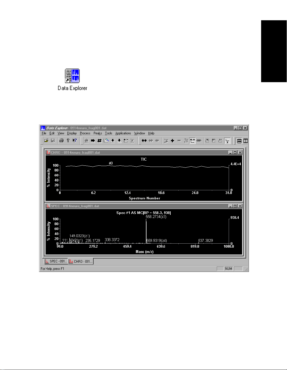
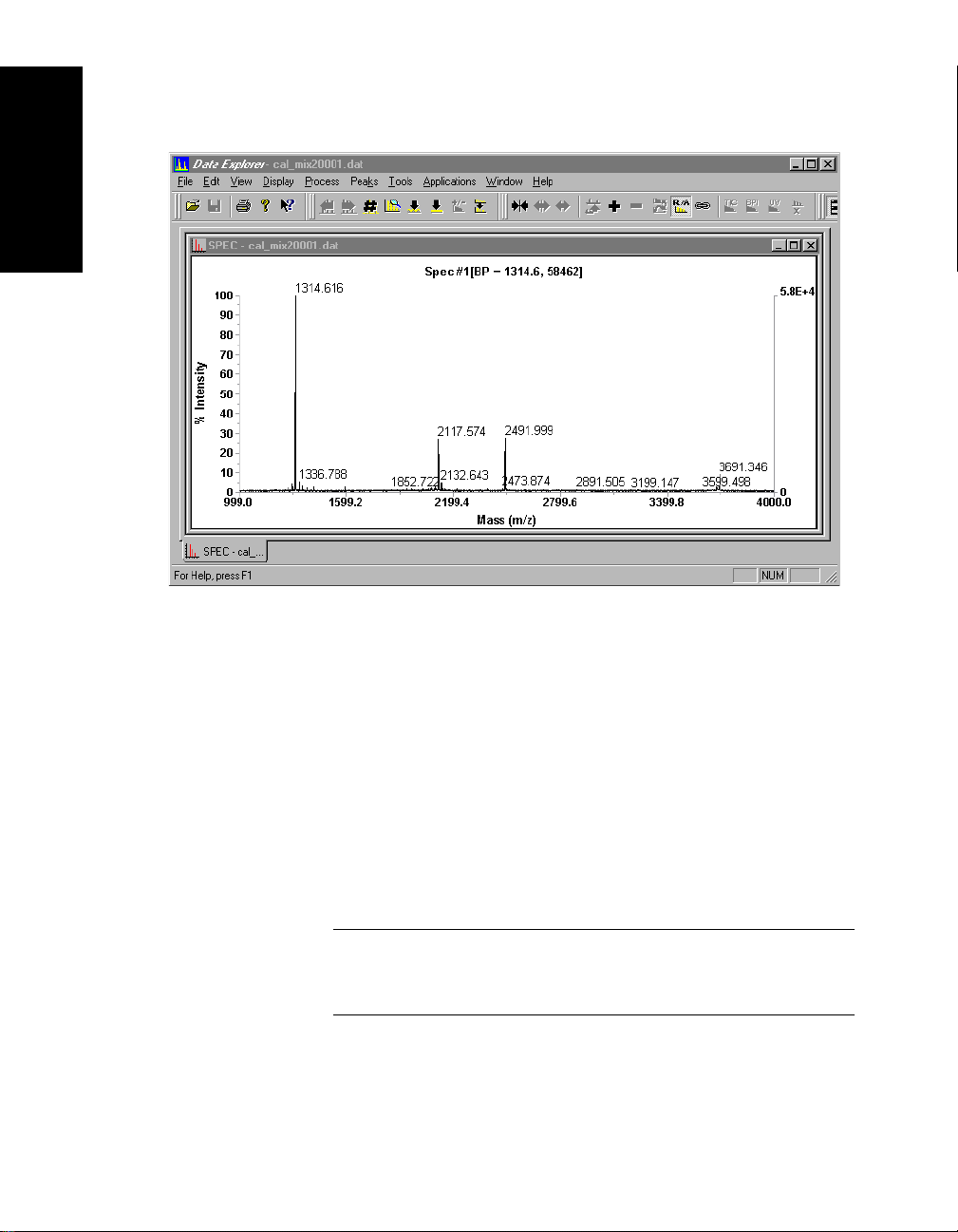
Figure 1-1 shows the Data Explorer main window with a Mariner data file open. Figure 1-2 shows the Data Explorer main window with a Voyager data file open.

To exit th e so ftw are, se lect Exit from the File menu in the Data Explorer window. The Data Explorer software closes.

Figure 1-1 Data Explorer Window with Mariner Data

™

Data Explorer

Software User’s Guide 1-3

Chapter 1 Data Explorer™ Basics

Figure 1-2 Data Explorer Window with Voyager Data

Default colors The default colors are different for Mariner and Voyager:

• Mariner—Black background, yellow traces, and green labels

• Voyager—White background, blue traces, and red labels

You can customize the default colors as needed. See Section 1.5.1, Changing Background Color.

NOTE: For consistency, all Mariner and Voyager screen examples in the following sections of this User’s Guide are shown with a white background.

1-4 Applied Biosystems

File Formats and Types

1.2 File Formats and Types

This section describes:

• Software applications compati bility

• Data (.DAT) file format

1.2.1 Software Applications Compatibility

You can use the Data Explorer Macro Recorder function to create Visual Basic scripts to automate tasks. You can also use the Visual Basic Editor directly to create more complex programs customized to suit your needs. For more information, see Section 6.7, Using the Macro Recorder.

Additionally, you can convert data to ASCII format for import into other software applications or import ASCII results. For more information, see Section 1.6.3, Converting to and Exporting ASCII Data, and Section 1.6.4, Importing a Trace in ASCII Format.

1.2.2 Data (.DAT) File Format

.DAT file format Data generated by Mariner and Voyager systems is stored in

.DAT file format. The .DAT file format incorporates all information about how a data file was acquired and processed into a single file. This format improves data processing and data storage efficiency.

Data files can contain spectra from a single acquisition or from multiple acquisitions (for example, multiple spectral data from a Voyager acquisition or multiple injection results from a Mariner CombiSolv run).

™

Data Explorer

Software User’s Guide 1-5

Chapter 1 Data Explorer™ Basics

Mariner .SPC file

format

Voyager .MS file

format

Extracting

information from

.DAT files

Table 1-1 Information Stored In a .DAT File

In Mariner software versions earlier than version 3.0, data files are stored in .SPC format. You can view and process .SPC files in Data Explorer, or you can convert these files to .DAT format. For information about the differences between the .DAT and the .SPC formats, see the Mariner User’s Guide.

In Voyager software versions earlier than version 5.0, data files are stored in .MS, .MSF, .MSA, and .MSB format. You can view and process .MS, .MSF, .MSA, and .MSB files in Data Explorer. You cannot convert them to .DAT format.

NOTE: Voyager .SPC format files are not s upported in the Data Explorer software.

You can also store parameter settings in separate files by extracting information from a .DAT file as needed for use with other files. For more information, see Section 1.6.5, Extracting and Saving Information from .DAT, .RSD, and .RCD Files.

The types of information stored in a .DAT file are described below.

™

Workstation

Category File Type File Content

Settings .BIC Instrument settings for controlling the operation of the

mass analyzer. For more information, see the:

• Mariner Workstation User’s Guide

• Voyager Biospectrometry Workstation User’s

Guide

1-6 Applied Biosystems

Table 1-1 Information Stored In a .DAT File (Continued)

Category File Type File Content

File Formats and Types

Settings

(continued)

Display .LBC Chromatogram label information. See Section 3.5.3,

Process .CAL Calibration constants generated by mass calibration.

.MSM (Mariner only)

.SET Graphic and processing settings. See Section 1.4.2,

.LBS Spectrum label information. See Section 3.5.3, Setting

MS Method settings, if data was acquired using an .MSM file.

NOTE: To access the instrument settings used to acquire each spectrum in an MS Method, you must first extract the .MSM file from the data file, then export the .BIC files from the .MSM file using the Export button in the MS Method editor. For more information on exporting a .BIC file from an .MSM file, see the Mariner Workstation User’s Guide.

Customizing Processing and Graphic Settings (.SET).

Setting Custom Peak Labels.

Custom Peak Labels.

For more information, see “Exporting .BIC, .MSM, and .CAL files” on page 1-36, and “Applying new constants to additional files” on page 5-16.

.CTS Processed trace that you access by selecting

Processing History from the Display menu. For information, see Section 2.4.7, Recalling and Rearranging Traces (Processing History).

NOTE: You select the name of the trace from the Processing History menu. You do not directly select a .CTS file. To purge or disable .CTS files, see “Setting Processing History options” on page 2-23.

™

Data Explorer

Software User’s Guide 1-7

Chapter 1 Data Explorer™ Basics

Additional files

types

Category File Type File Content

Data .PKT Text file containing a chromatogram or a spectrum peak

.TXT Data file exported to an ASCII text file. See

Data .SPC

(Mariner only)

.MS (Voyager only)

Additional file types you may see on your system are described below.

Table 1-2 Additional File Types

list that you can save from the Output window. See “Output window” on page 1-15.

Section 1.6.3, Converting to and Exporting ASCII Data. Data file format for files acquired before Version 3.0 of

the Mariner Instrument Control Panel.

NOTE: Voyager data files in .SPC format have a file structure different from Mariner data files in .SPC format, and are not supported in the Data Explorer software.

Data file format for files acquired before Version 5.0 of the Voyager Instrument Control Panel.

.MSA and .MSF (Voyager only)

.MSB (Voyager only)

Procedure .TUN

(Mariner only)

1-8 Applied Biosystems

PSD data file format for composite and fragment files acquired before Version 5.0 of the Voyager Instrument Control Panel.

NOTE: The Data Explorer software cannot generate composite spectra from .MSF fragment files.

Baseline-corrected data file format for composite and fragment files acquired before Version 5.0 of the Voyager Instrument Control Panel.

AutoTune method. See the Mariner Workstation User’s

Guide.

File Formats and Types

Table 1-2 Additional File Types (Continued)

Category File Type File Content

Reference .REF List of masses to select from during calibration. See

“Creating and saving a calibration reference file” on page 5-18.

Process .RCT

(Mariner only)

.RST Results file saved from:

Results file saved from:

• Mariner .SPC format data file (versions earlier than 3.0) in the Data Explorer software after a chromatogram is manually processed.

See Section 2.8, Saving, Opening, and Deleting .SPC Results Files (Mariner Data Only).

• Mariner .DAT format data file (version 3.0 and later) in the Mariner Instrument Control Panel for a snapshot of chromatogram data.

NOTE: Results for a .DAT file are stored within the .DAT file, not as a separate file.

• Mariner .SPC format data file (versions earlier than 3.0) in the Data Explorer software after a spectrum is manually processed.

See Section 2.8, Saving, Opening, and Deleting .SPC Results Files (Mariner Data Only).

• Voyager .MS format data file in the Data Explorer software after a spectrum is manually processed.

• Mariner .DAT format data file (version 3.0 and later) in the Mariner Instrument Control Panel for a snapshot of spectrum data.

NOTE: Results for a .DAT file are stored within the .DAT file, not as a separate file.

Data Explorer

™

Software User’s Guide 1-9

Chapter 1 Data Explorer™ Basics

Table 1-2 Additional File Types (Continued)

Category File Type File Content

Process

(continued)

.RCD Chromatogram results file exported from .DAT files. See

Section 2.7, Exporting, Opening, and Deleting .RCD and .RSD Results Files (Mariner Data Only).

.RSD Spectr um results file exported from .DAT files. See

Section 2.7, Exporting, Opening, and Deleting .RCD and .RSD Results Files (Mariner Data Only).

1-10 Applied Biosystems

1.3 Parts of the Data Explorer Window

This section describes:

• Overview

• Toolbar

• Chromatogr am and Spe ctru m windows

• Tabs for data files

• Data file names

• Output window

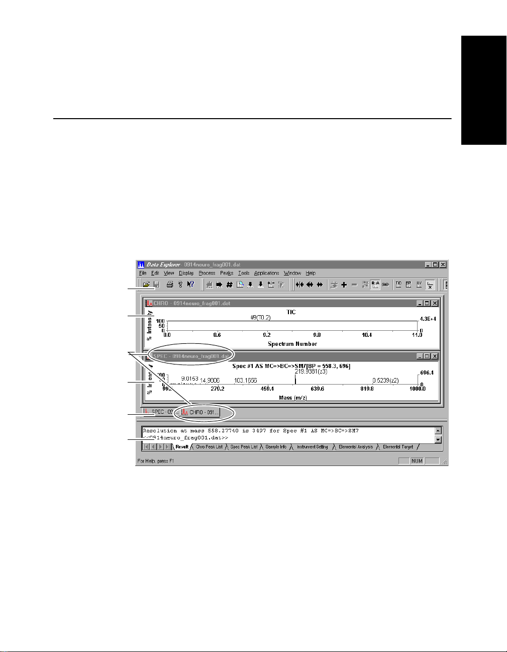
Overview Figure 1-3 shows the Data Explorer window with Mariner data.

Toolbar

Chromatogram

window

Parts of the Data E xplorer Window

Data file name

Spectrum

window

Tabs for

open data files

Output

window

Figure 1-3 Parts of the Data Explorer Window

™

Data Explorer

Software User’s Guide 1-11

Chapter 1 Data Explorer™ Basics

Toolbar The toolbar contains buttons that access Data Explorer

functions. For a description of a toolbar button, place the cursor on the

button. A brief description of the button (ToolTip) is displayed below the button.

For information on adding or removing toolbar buttons, see “Customizing toolbars” on page 1-21.

Chromatogram

and Spectrum

windows

Table 1-3 Mariner Data Displayed in Chromatogram and Spectrum Windows

Window Mariner Data

CHRO Displays:

• Total Ion Chromatogram—Includes the entire mass range saved in the data file.

• Extracted Ion Chromatogram (XIC) (optional)—Includes only the signal response from a mass window or range

• Constant Neutral Loss Chromatogram (CNL) (optional)—Extr a c ts only the response from peaks that are separated by a selected mass difference.

Optionally displays the following from Diode Array data (DAD):

• Total Absorbance Chromatogram (TAC)

• Channel (Ch)

• Extracted Absorbance Chromatogram (XAC)

Can be displayed as % Intensity versus Retention Time or Spectrum number by selecting Traces from the Display menu, then selecting X Axis In, then selecting Spectrum Number or Time.

Refer to the following tables for descriptions of the types of data that you can display in the Chromatogram (CHRO) and Spectrum (SPEC) windows:

• Mariner data—Table 1-3

• Voyager data—Table 1-4

1-12 Applied Biosystems

Parts of the Data E xplorer Window

Table 1-3 Mariner Data Displayed in Chromatogram and Spectrum Windows

(Continued)

Window Marin er D ata

SPEC Displays the spectrum for the selected time in the TIC or TAC trace. By

default, displays spectrum #1. The trace label includes “DAD” for spectra selected from TAC.

Indicates Base Peak (BP) mass and intensity for the tallest peak in the spectrum. Displayed as % Intensity versus Mass-to-Charge (m/z). The right axis is scaled to the intensity of the base peak.

Table 1-4 Voyager Data Displayed in Chromatogram and Spectrum Windows

Window Voyager Data

CHRO Window is not displayed by default.

Optionally displays Total Ion Current (TIC) for multiple spectra .DA T files if you select Restore Chromatogram from the View menu.

NOTE: DAD functions are not supported for Voyager data.

SPEC Depends on the type of data file you open:

• Single spectrum files—Displays the spectrum and labels the plot as spectrum #1.

• Multiple spectrum files—Displays the spectrum for the selected time in the TIC trace (if displayed). By default, displays spectrum #1.

• PSD files—Displays the composite spectrum and labels it as Stitched PSD. You can display segment spectra by clicking

and .

Indicates Base Peak (BP) mass and intensity for the tallest peak in the spectrum. Displayed as % Intensity versus Mass-to-Charge (m/z). The right axis is scaled to the intensity of the base peak.

Data Explorer

™

Software User’s Guide 1-13

Chapter 1 Data Explorer™ Basics

Labels in the chromatogram or spectrum title identify the type of data displayed in the window. For a description of labels, see Section 2.4.10, Viewing Trace Labels.

For more information on Chromatogram and Spectrum windows, see Chapter 2, Using Chromatogram and Spectrum Windows.

Context-sensitive

menus

The commands displayed on the menus in the Data Explorer window depend on the window that is active when you select the menu:

• Only Mariner-related commands are displayed on menus when you open a Mariner .DAT file.

• Only Voyager-related comma nds are displ ay ed on menus when you open a Voyager .DAT file.

• Only spectrum-related commands are displayed if you select menus when the Spectrum window is active.

• Only chromatogram-related commands are displayed if you select menus when the Chromatogram window is active. For Voyager multiple spectra .DAT files, UV functions are disabled.

Tabs for data files Chromatogram and Spectrum windows display a tab at the

bottom (see Figure 1-3 on page 1-11) that allow you to switch between data files, or between Chromatogram and Spectrum windows for a Mariner data file. See “Moving Between Open Files” on page 2-8.

Data file names Data file names are displayed in the:

• Title bar of each window

• Tab for each window

1-14 Applied Biosystems

NOTE: If the full name of the data file does not fit in the tab, part of the name is displayed followed by “...”. To display the full name of the data file, place the cursor on the tab. The full name of the data file is displayed below the tab.

Parts of the Data E xplorer Window

Output window The Output window (see Figure 1-3 on page 1-11) displays

tabs at the bottom that you can click to switch between the types of information displayed:

Output wind ow

tabs

• Result—Displays results generated using commands on the Process, Tools, and Applications menus. For more information on results, see:

• Section 5.3, Manual Calibration, or Section 5.4, Automatic Calibration

• Section 5.6, Mass Deconvolution (Mariner Data Only)

• Section 6.2, Using the Isotope Calculator

• Section 6.3, Using the

Mass Resolution Calculator

• Section 6.4, Using the Signal-to-Noise Ratio Calculator

• Chro Peak List —Displays results of chromatogram peak detection and integration. For more information, see Section 3.3, Peak List.

• Spectrum Peak List—Displays results of spectrum peak detection, integration, and centroiding. For more information, see Section 3.3, Peak List.

• Sample Info—For data files, displays the:

• Software version used for acquisition

• Acquisition time and sample comments entered

when data was acquired

For result files (.RCT, .RST, .RCD, .RSD), displays any processing functions that have been performed and saved in the result file.

™

Data Explorer

Software User’s Guide 1-15

Chapter 1 Data Explorer™ Basics

• Instrument Setting—Displays a list of instrument settings used to obtain the data. The settings are taken from instrument settings pages in the Instrument Control Panel. Also displays segments, event numbers, and event tags from Mariner MS Method acquisitions and LC information if LCMS was acquired using Mariner.

• Elemental Analysis—Displays results for the Elemental Composition calc ula tor. For information, see Section 6.1, Using the Elemental CompositionCalculator.

• Elemental Targeting—Displays results for the Elemental Targeting application. For information, see Section 6.6, Using the Elemental Targeting Application.

Displaying,

clearing, and

closing

The Output window is automatically displayed when you generate results (for example, when you calculate resolution).

To display the Output window manually, select Output Window from the View menu.

To clear the Output window, right-click the Output window, then select Clear Window.

To close the Output window, deselect Output Window from the View menu, or right-click the Output window, then select Hide.

Hint: To maximize the Chromatogram and Spectrum windows after hiding the Output window, click or in the toolbar.

1-16 Applied Biosystems

Customizing the Data Explorer Window

1.4 Customizing the Data Explorer Window

This section includes:

• Setting default values

• Customizing Graphic and Processing settings

• Customizing toolbars

1.4.1 Setting Default Values

You can set defaults for most dialog boxes in the Data Explorer software by setting a value or selecting a button, closing the dialog box, then closing the data file you are viewing.

The next time you open the dialog box, the last settings specified are displayed.

1.4.2 Customizing Processing

and Graphic Settings (.SET)

This section includes:

• Overview of processing and graphic settings

• What settin gs contain

• Default processing and graphic settings

• Default graphic settings

• Customizing settings saved in a data file

• Making a copy of default .SET files before customizing

• Opening, customizing, and saving .SET files

• Applying a .SET file

™

Data Explorer

Software User’s Guide 1-17

Chapter 1 Data Explorer™ Basics

Overview of

processing and

graphic settings

What settings

contain

Processing and graphic settings control how data is processed and displayed in the Data Explorer software. The last settings used are automatically saved in the data file when you close it. The next time you open the data file, you can select any of the following to apply:

• Settings from the data file—Described in Sect ion 2.1, Opening and Closing Data Files.

• Default settings—Described below.

• Settings from a selected set file—You can also apply

processing and graphic settings that have been exported as stand-alone .SET files from other data files. See “Applying a .SET file” on page 1-20.

Graphic settings include the attributes you set in Graphic Options, described in Section 1.5, Setting Graphic Options.

Processing settings include:

• Peak detection parameters, described in Section 3.2.4, Peak Detection Parameter Descriptions

• Smoothing points, described in Section 5.7, Noise Filtering/Smoothing

• Automatic calibration settings, described in Section 5.4, Automatic Calibration

Default

processing and

graphic settings

1-18 Applied Biosystems

NOTE: You can open a .SET file in Microsoft Notepad to view the complete file contents.

The following default settings files (stand-alone .SET files) that contain both processing and graphic settings are provided on your system in the C:\MARINER\PROGRAM\Set Files directory or the C:\VOYAGER\PROGRAM\Set Files directory:

• MARINER.SET

• VOYAGERLINEAR.SET

• VOYAGERREFLECTOR.SET

• VOYAGERPSD.SET

For more information on Peak Detection settings, see Section 3.7, Default Peak Detection Settings .

Customizing the Data Explorer Window

Additional .SET files that have been developed for detection of different types of data are included in the C:\VOYAGER\PROGRAM\SET FILES directory . The names of the .SET files indicate the type of data the files can be used for.

The appropriate default settings for the type of data you open are automatically applied to a data file the first time you open it in Data Explorer. You can also manually apply these settings if desired. For information, see “Applying a .SET file” on page 1-20.

Default graphic

settings

Customizing

settings saved in

a data file

Making a copy of default .SET files

before

customizing

Two additional default settings files (stand-alone .SET files) that contain graphic settings only are also provided on your system in the C:\MARINER\PROGRAM directory or the C:\VOYAGER\PROGRAM directory:

• DEFAULTWHITE.SET

• DEFAULTBLACK.SET

These .SET files contain the default graphic settings applied when you select White Backgr ound or Dark Background (after selecting Default from the Display menu). For information, see Section 1.5.1, Changing Background Color.

You can customize settings saved in a data file by adjusting graphic or processing settings in the Data Explorer window.

Settings are saved with a data file when you close the data file, and are automatically applied the next time you open the data file, if specified. For more information, see Section 2.1, Opening and Closing Data Files.

You can also save the settings in a .SET file for use with other data files, as described in “Saving .SET files” on page 1-37.

All .SET files are user editable. However, before you edit the default pr oc es si ng / g ra ph ic . SE T fi l e s (s ee page 1-18), m ak e a copy of the original .SET file, in case you need to reload the settings for default peak detection. Copy the file using Windows NT

Explorer.

Data Explorer

™

Software User’s Guide 1-19

Chapter 1 Data Explorer™ Basics

Opening,

customizing, and

saving .SET files

To open, customize, and save .SET files:

1. If you are customizing a default .SET file, make a copy of the original file before opening it. See “Making a copy of default .SET files before customizing” on page 1-19.

2. Select Settings from the File Menu.

3. Select one of the foll owing:

• Restore Processing Settings

• Restore Graphic Settings

• Restore Graphic/Processing Settings

4. In the Restore dialog box, select or type the name of the .SET file, then click OK.

5. Customize processing and graphic settings as needed. For information on the contents of processing and graphic settings, see “What settings contain” on page 1-18.

6. To save settings, select S ettin gs from the File menu, then select one of the following:

• Save Processing Settings As

• Save Graphic Settings As

• Save Graphic/Processing Settings As

7. In the Save As dialog box, type the name of the .SET file, then click OK.

Applying a .SET

file

1-20 Applied Biosystems

You can apply a .SET file two ways:

• Select Recent Processing Settings from the File menu, then select a .SET file from the list of most recently used files

NOTE: When you apply a .SET file from the Recent Processing Settings menu, only the process settings are applied.

• Select an option from the Settings command on the File menu

To use the Settings option:

Customizing the Data Explorer Window

1. Select Settings from the File menu.

2. Select one of the following:

• Restore Processing Settings

• Restore Gra ph ic Set tin gs

• Restore Graphic/Processing Settings

• Revert to the Last Saved Graphic/Processing

Settings

3. If you select a Restore Settings option, select or type the name of the .SET file in the Restore dialog box, then click OK.

Hint: You can also restore default processing and graphic settings when you open a file or files. See Section 2.1, Opening and Closing Data Files.

1.4.3 Customizing Toolbars

Customizing

toolbars

To customize the toolbar:

1. Select Customize Toolbar from the Tools menu to display the Customize dialog box.

2. To display or hide a toolbar section, click the Toolbars tab, then select or deselect a toolbar.

3. To add a button to a toolbar, click the Commands tab, select the appropriate category, then click-drag the button to any toolbar in the main toolbar.

Hint: To display a button description, click the button within the Customize dialog box. You can add buttons from any category to any toolbar. For example, you can add buttons from the File category to the Graph toolbar.

™

Data Explorer

Software User’s Guide 1-21

Chapter 1 Data Explorer™ Basics

4. To remove a button from a toolbar, click-drag the button

from the toolbar.

NOTE: The Customize dialog box must be displayed to click-drag a button from a toolbar.

5. Click OK to close the Customize dialog box.

Undocking

toolbars

Creating

toolbars

The toolbar at the top of the Data Explorer window is divided into sections. A section is preceded by a double vertical bar.

You can move (undock) each section of the toolbar within the Data Explorer window by click-dragging the double bar at the left side of the toolbar section.

To move the toolbar section back to the top of the window, click-drag the toolbar back to the original position.

You can display or hide each section individually, add or remove buttons on the toolbar, and rearrange the order of buttons displayed. To do so, you must have the Customize dialog box open, as described in the previous section.

You can create new toolbars by click-dragging buttons to a window area where there is no toolbar. You can then add buttons to the new toolbar as described in “Customizing toolbars” on page 1-21.

1-22 Applied Biosystems

Setting Graphic Options

1.5 Setting Graphic Options

This section includes:

• Changing back ground color

• Customizing options

• Reverting to previous graphic options

NOTE: Changes you make to Graphic Options are saved with the data file.

1.5.1 Changing Background Color

White or dark

background

You can switch background color by selecting Default from the Display menu, then selecting:

• White Background—Displays blue traces and red labels by default. Default settings are contained in DEFAULTWHITE.SET.

• Dark Background—Displays yellow traces and green labels by default. Default settings are contained in DEFAULTBLACK.SET.

NOTE: These .SET files contain graphic settings only. They do not contain processing settings.

You can customize the graphic settings associated with default settings if desired. For information, see Section 1.4.2, Customizing Processing and Graphic Settings (.SET).

Data Explorer

™

Software User’s Guide 1-23

Chapter 1 Data Explorer™ Basics

1.5.2 Customizing Graphic Options

This section includes:

• Accessing graphic option s

• Setting colors

• Setting line widths

• Setting data cursors

• Setting traces in line or bar mode

• Setting graphic compression

Accessing

graphic options

To access graphic options:

1. Display the trace of interest.

2. From the Display menu, select Graphic Options.

3. To use the graphic options settings for all traces, click Use same settings for all traces in the View Setup tab.

4. Click a Graph Setup tab in the Graph and Plot Options dialog box (Figure 1-4).

5. Set colors, line widths, data cursors, and graphic compression as described in the following sections.

6. Click OK.

1-24 Applied Biosystems

Line or vertical

bar traces Line width

Data cursor

Setting Graphic Options

Peak bounds

Graphic

compression

Figure 1-4 Graphic Options Dialog Box—

Graph Setup Tab

Setting colors You can set colors manually or automatically.

Manually To manually select the color of graph features (axis, peak

bounds, tick labels, data cursor) and plot features (traces, peak labels):

1. Select Graphic Options from the Display menu.

2. Set colors in the Graph Setup tab (see Figure 1-4).

™

Data Explorer

Software User’s Guide 1-25

Chapter 1 Data Explorer™ Basics

When you manually set colors, note:

• Selections set to white (or line widths set to 0) may not print on certain printers.

• If you select different trace colors for multiple traces, only the color for the active trace is saved when you close the data file.

Automatically

using Auto Color

Setting line

widths

Automatically assigning trace colors is useful when overlaying traces. To automatically assign trace colors:

1. Select Graphic Options from the Display menu.

2. Select Auto Color in the View Setup tab. The software assigns and displays trace colors when the traces are overlaid.

When you use Auto Color:

• The active trace color stays at its original setting.

• Other trace colors are set based on the active trace color.

For example, if the active trace is yellow, other traces are assigned the colors pale blue, pale green, and medium gray, which are the colors listed after yellow in the Trace color list, excluding whit e.

NOTE: White is not used in Auto Color because white may not print on certain printers.

Y ou can control trace appearance by setting line widths. To set line widths:

1. Select Graphic Options from the Display menu.

1-26 Applied Biosystems

2. Set line width in the Plot Setup section of the Graph Setup tab (see Figure 1-4 on page 1-25).

NOTE: Line Widths of 0 or 1 (or lines set to the color white) may not print on certain printers. If traces do not print, change the line width (or color).

Setting Graphic Options

Setting data

Label

Type

cursors

To enable data cursors and set cursor labels and attributes:

1. Select Graphic Options from the Display menu.

2. In the Data Cursor section of the Graph Setup tab (see

Figure 1-4 on page 1-25), select Show Data Cursors, then select one of the following cursors from the Type drop-down list:

• X—Single vertical cursor

• Y—Single horizontal cursor

• X-Y—Vertical and horizontal cursors

• X-X—Two vertical cursors

• X-Y-X—Two vertical cursors and one horizontal cursor

NOTE: If data cursors are displayed, they are printed when you print traces. To suppress data cursor printing, deselect Show Data Cursors before printing.

To set the cursor mode, select the appropriate label type as described below:

Options

Y Label • Absolute—Displays the number of counts.

• BP Relativ e —Displays the % Intensity value relative to the base peak in the trace. Includes “BP%” marker on the cursor label.

• Display Relative—Displays the % Intensity value relative to the

largest peak in the current display range.

X-X

Label

• Absolute—Displays the Spectrum Number or Retention Time (chromatogram) or the Mass (spectrum).

• X-Relative—Available if you have two X cursors displayed. For the first cursor, displays the Spectrum Number or Retention Time (chromatogram) or the Mass (spectrum). For the second cursor, displays the appropriate value relative to the first cursor.

For example, if you place the first X cursor in a spectrum at 100 m/z and the second X cursor at 80 m/z, the cursors are labeled 100 and –20.

™

Data Explorer

Software User’s Guide 1-27

Chapter 1 Data Explorer™ Basics

Setting traces in

Line or Vertical

Bar mode

Setting graphic

compression

You can change the trace display from Line to Vertical Bars. Each vertical bar represents one data point.

Vertical bar mode is useful when setting peak detection parameters to determine the number of points across a peak.

NOTE: Graphic Compression mode is not saved as part of graphic settings. When you close a data file, it is automatically reset to the default Local Max setting.

By default, all data is compressed when it is displayed on your computer screen. The degree of compression is determined by the number of data points in the data file and the resolution setting of your computer monitor.

For example, assume that a data file contains 10,000 data points and needs compression to 1,000 data points to fit on your computer screen. Every 10 data points will be compressed into a single data point.

To set graphic compression settings:

1. Select Graphic Options from the Display menu.

2. In the Graph Setup tab of the Graph and Plot Options dialog box (see Figure 1-4 on page 1-25), select a Graphic Compression mode :

1-28 Applied Biosystems

• Local Max (default)—Uses the maximum data point within the range of data points being compressed (range of 10 in the example above).

• Average—Uses the average of the data points within the range of data points being compressed (range of 10 in the example above).

• Sum (Binning)—Uses the sum of the data points within the range of data points being compressed (range of 10 in the example above).

NOTE: Changing the graphic compression mode may alter the displayed intensities of peaks in a trace.

Setting Graphic Options

1.5.3 Reverting to Previous Graphic Options

You have two options to revert to previously used graphic options:

• Revert to Last Saved Graphic Setting—Reverts to the last graphic settings saved in the data file. Does not affect processing settings.

To access, select Default from the Display menu, then select Revert to Last Saved Graphic Setting.

• Revert to Last Saved Graphic/Processing Settings—Reverts to the last graphic and processing

settings saved in the data file. To access, select Settings from the File menu, then

select Revert to Last Saved Graphic/Processing Settings.

Hint: Instead of applying the settings saved with a data file, you can apply the default settings stored in the default .SET file for your system (see page 1-18). To apply the default settings, close the data file, open the data file again, then select Use Default Settings in the Open dialog box. For more information, see Section 2.1, Opening and Closing Data Files.

Data Explorer

™

Software User’s Guide 1-29

Chapter 1 Data Explorer™ Basics

1.6 Managing Files

This section describes:

• Converting .SPC file format to .DAT file format (Mariner only)

• Converting data from profile to centroid (Mariner only)

• Converting to and exporting ASCII data

• Importing a trace in ASCII format

• Extracting and saving information from .DA T, .RSD, and

.RCD files

• Copying from data files

1.6.1 Converting .SPC File Format to .DAT File Format (Mariner Data Only)

This section includes:

• When to convert

• Before you begin

• Converting

• Viewing file properties

• Searching file properties

NOTE: You cannot convert Voyager .MS files to .DAT format.

When to convert You are not required to convert Mariner .SPC file format (for

data acquired in software versions earlier than 3.0) to .DA T file format. However, the .DAT format allows you to store all information associated with the file (such as data, results, settings) in one file, simplifying file management.

1-30 Applied Biosystems

Managing Files

Before you begin Confirm that the .SPC and .CGM files are located in the

same directory. Use Windows NT directory contents and to move the .SPC and .CGM files as necessary. If the .SPC and .CGM files are not in the same directory, when you open the .SPC file, a “Failed to open chromatogram data” message is displayed.

To check that the .SPC and .CGM files are in the same directory:

1. Select Open from the File menu. The Open dialog box is displayed.

2. From the Files of type drop-down list, select All Files (*.*). A list of all files contained in the directory is displayed.

3. Check that the .SPC and .CGM files are present.

Explorer to display the

Converting In the Data Explorer window:

1. Open or click the .SPC file to convert.

2. Select Convert from the File menu.

3. Select New Dat a Fo rmat. The Convert to .DAT Format dialog box is displayed

(Figure 1-5).

Figure 1-5 Convert to .DAT Format Dialog Box

4. To add file property information (for example, Title, Author, or Keywords) to the file, click Set Property, enter the appropriate information, then click OK. For more information, see “Viewing file properties” on page 1-32.

™

Data Explorer

Software User’s Guide 1-31

Chapter 1 Data Explorer™ Basics

The Convert to .DAT Format dialog box reappears.

5. Click OK. A message box is displayed, showing the file name of

the newly created .DAT file.

6. Close the .SPC file and open the .DAT file before processing. If desired, manually delete the .SPC file and associated files.

Viewing file

properties

Searching file

properties

File properties are accessible in Windows NT Explorer and provide general information about a data file without opening the file in the Data Explorer software.

To view file properties:

1. In Data Explorer, close the file of interest.

2. In Windows NT Explorer, select the file, then right-click.

3. Select Properties from the menu.

4. Click the Summary tab.

NOTE: If the Summary tab is not available, the file may be open in Data Explorer. Close the file and repeat the steps above.

To search for a file based on file properties:

1. In Windows NT Explorer, select Find from the Tools menu, then select Files or Folders.

The Find: All Files dialog box is displayed.

2. In the Name & Location tab, type or select a directory in the Look in text box.

1-32 Applied Biosystems

3. Select the Advanced tab.

4. Select Data Explore Document from the Of type drop-down list.

5. Type the information you are searching for (for example, a title or keyword) in the Containing text box, then click Find Now.

Managing Files

1.6.2 Converting Data from Profile to Centroid (Mariner Data Only)

Overview You can convert an entire data file from profile to centroid

format. Centroid format files are smaller than profile format files.

NOTE: Profile data is not automatically deleted when you convert to centroid data. You can delete the profile data file using Windows NT Explorer.

Before you begin If the file to convert is in .SPC format, confirm that the .SPC

and .CGM files are located in the same directory. For information see “Before you begin” on page 1-31. If the .SPC and .CGM files are not in the same directory, when you open the.SPC file, a “Failed to open chromatogram data” message is displayed.

Converting to

centroid

To convert from profile to centroid format:

1. Open or activate the .DAT or .SPC file to convert.

2. Select Convert from the File menu, then select Centroid. The Save As dialog box is displayed. The software

appends a “-CT” suffix to the file name. This is the default file name. You can enter a new file name for the centroid file.

3. Click Save.

NOTE: The m/z range in a data file that is converted from profile to centroid is determined by the peak detection range set in Data Explorer, not the m/z range in the original data file. For more information, see Section 3.2, Peak Detection.

™

Data Explorer

Software User’s Guide 1-33

Chapter 1 Data Explorer™ Basics

1.6.3 Converting to and Exporting ASCII Data

This section describes:

• Converting a data file to ASCII format

• Exporting a trace to ASCII format

Converting a data

file to ASCII

format

Exporting a trace

to ASCII format

Y ou can convert a data file for use in a spreadsheet or another application and export and import single traces in ASCII format.

To convert an entire active data file to an ASCII text file:

1. Open the data file to convert.

2. Fr om the File menu, select Convert, then select ASCII text.

A Save As dialog box is displayed.

3. Specify the name and destination for the file to be exported. By default, the software assigns a .TXT extension to the file.

4. Click OK.

You can export a selected trace to ASCII format for display in Data Explorer software or for use in another application.

To export trace data to ASCII format:

1. With a data file open, select the trace window.

2. Fr om the File menu, select Export, then select Chromatogram or Spectrum (the menu item is context sensitive).

1-34 Applied Biosystems

A Save As dialog box is displayed.

3. Specify the name and destination of the file to be exported. By default, the software assigns a .TXT extension to the file.

4. Click OK.

Managing Files

1.6.4 Importing a Trace in ASCII Format

You can import trace data in ASCII format. If the file you are importing was originally exported using the Data Explorer software, you can import a spectrum trace only into the Spectrum window and a chromatogram trace only into the Chromatogram window. However, if the data is from another source, the software does not know the data type and you must make sure to import the data into the correct window type.

Importing a Trace

in ASCII Format

To import an ASCII trace:

1. Open a data file and activate a Chromatogram or Spectrum window.

NOTE: You must open a data file before you can import ASCII data, even if the data file is unrelated to the imported data.

2. Select Add/Remove Traces from the File menu, then set the Replace Mode by selecting one of the following:

• Replace the Active Trace

• Add a New Trace

3. From the File menu, select Import, then select ASCII Chromatogram or ASCII Spectrum (the menu item is

context sensitive to the selected window). An Open dialog box appears.

4. Select the ASCII file to import.

5. Click OK. The imported trace is displayed in the active window.

Data Explorer

™

Software User’s Guide 1-35

Chapter 1 Data Explorer™ Basics

CAUTION

An imported ASCII format trace contains only the data points for the trace. The Sample Info and Instrument settings tabs in the Output window display data from the data file you opened in step 1. These tabs do not include information about the imported trace.

1.6.5 Extracting and Saving Information from .DAT, .RSD, and .RCD Files

Overview You can extract the following information from a .DA T data file,

.RSD spectrum results file, and .RCD chromatogram results file, then save the information as a stand-alone file for use with other files:

• Instrument settings (.BIC)

• MS Method (.MSM) (Mariner data only)

• Calibration constants (.CAL)

• Processing/graphic settings (.SET)

• Spectrum or chromatogram peak labels (.LBS or .LBC)

• ASCII Spectrum and ASCII Chromatogram (.TXT)

Exporting .BIC,

.MSM, and .CAL

files

1-36 Applied Biosystems

To export Instrument settings (.BIC), MS Method settings (.MSM), or calibration constants (.CAL) from a .DAT or results file:

1. Open or activate the data (.DAT) or results (.RSD or .RCD) file.

2. Fr om the File menu, select Export, then select:

• Calibration—To export the last applied calibration constants in a .CAL file.

Managing Files

NOTE: To export calibration constants used to acquire the data, select Mass Calibration from the Process menu, then select the Revert to Instrument Calibration before exporting. For more information, see Section 5.3.4, Reverting to Instrument Calibration.

• Configuration—To export .BIC or .MSM files (.MSM—Mariner data only).

NOTE: To access the instrument settings for each spectrum in a data file acquired using a Mariner MS Method, you must first extract the .MSM file from the data file as described above. Then export the .BIC files from the .MSM file using the Export button in the MS Method editor. For more information on exporting a .BIC file from .MSM, see the Mariner Wo rks tati on U ser’s Guide.

3. In the Save As dialog box, type a name for the exported file, then click Save.

Saving .SET files To sa ve proces sing and graphic s ettings ( .SET) from a .DAT or

results file:

1. Open or activate the .DAT, .RSD or .RCD file.

2. From the File menu, select Settings, then select one of the following:

• Save Processing Settings As

• Save Graphic Settings As

• Save Graphic/Processing Settings As

3. In the Save As dialog box, type a name for the .SET file, then click OK.

For information, see Section1.4.2, Customizing Processing and Graphic Settings (.SET).

™

Data Explorer

Software User’s Guide 1-37

Chapter 1 Data Explorer™ Basics

Saving .LBS

and .LBC files

To save spectrum (.LBS) or chromatogram (.LBC) peak label files from a .DAT, .RSD, or .RSC file, see Section 3.5.3, Setting Custom Peak Labels.

1.6.6 Copying from Data Files

Overview You can copy the following types of data from data and result

files to the Windows clipboard:

• Trace Image—Copies the graphic image of the trace in the active window.

• Trace Data—Copies the raw data for the trace displayed in the active window. You can also use this command by right-clicking, then selecting Copy Trace Data. For more information, see Section 2.5.2, Copying Traces from Multiple Data Files to a Window.

• Displayed Peaks—Copies peak list entries for the peaks displayed in the active window.

• All Peaks—Copies peak list entries for all peaks in the active view.

• Mass List—Copies all centroid or apex masses fro m the peak list for the active Spectrum window.

Copy trace image To copy the trace as it is displayed in the active window to the

Windows clipboard:

1. Select the trace window to copy. Zoom and adjust the trace as needed.

2. From the Edit menu, select Copy, then select Trace Image.

3. Paste the image into an application that handles Windows Metafile format images, for example Microsoft PowerPoint

1-38 Applied Biosystems

Managing Files

NOTE: If you paste the image into an application that does not handle Windows Metafile format images, for example Microsoft Paint, images are distorted.

Copy trace data To copy raw data (x,y pairs) for the peaks displayed in the

active trace to the Windows clipboard:

1. Select the trace window to copy. Zoom and adjust the trace as needed.

NOTE: Only raw data for the set of peaks displayed in the trace window is copied.

2. From the Edit menu, select Copy, then select Trace Data.

3. Paste the data into an appropriate application, for example, another Data Explorer trace window or Microsoft Excel.

When pasted into a Data Explorer trace window, the trace appears with the filename in parentheses and the trace label from the copied trace.

CAUTION

A trace pasted into an active Data Explorer window contains only the data points for the trace. The Sample Info and Instrument settings tabs display data from the original data file. These tabs do not include information about the copied trace.

Copy displayed

peaks

Use this method to copy the section of the peak list pertaining to the peaks displayed in the active trace window. To copy the peak list for all peaks in the active trace, see “Copy all peaks” on page 1-40.

™

Data Explorer

Software User’s Guide 1-39

Chapter 1 Data Explorer™ Basics

NOTE: Copy Displayed Peaks copies all fields and

headings. However, some data applications may not work correctly if headings are present because the first row contains text and not data. For information on copying the peaks list without headings, see Section 3.3.3, Saving the Peak List.

To copy the peak list for the displayed peaks to the Windows clipboard:

1. Set peak detection as needed to create a peak list. See Section 3.2, Peak Detection.

2. Select the trace window to copy. Zoom and adjust the trace as needed.

NOTE: Only peak list information for the set of peaks displayed in the trace window is copied.

3. From the Edit menu, select Copy, then select Displayed Peaks.

4. Paste the data into an appropriate application, for example Microsoft Excel.

Copy all peaks Use this method to copy the peak list for all peaks in the active

trace. T o copy only the section of the peak list pertaining to the peaks displayed in the active trace window, see “Copy displayed peaks” on page 1-39.

NOTE: Copy All Peaks copies all fields and headings. However, some data applications may not work correctly if headings are present because the first row contains text and not data. For information on copying the peaks list without headings, see Section 3.3.3, Saving the Peak List.

To copy the peak list for all peaks in the active trace to the Windows clipboard:

1. Set peak detection as needed to create a peak list. See Section 3.2, Peak Detection.

1-40 Applied Biosystems

2. Select the trace window to copy.

Managing Files

3. Display the peak list by selecting Output Window from the Display menu, then clicking the Chro Peak List or Spec Peak List tab.

4. Sort the peak list as needed. See “Sorting the peak list” on page 3-42.

5. From the Edit menu, select Copy, then select All Peaks.

6. Paste the data into an appropriate application, for example, Microsoft Excel.

Copy mass list This function copies only the masses for the spectrum and is

useful for pasting data directly into spreadsheets or other applications without having to delete header information.

To copy all centroid or apex mass data from the spectrum peak list to the clipboard:

1. Select the Spectrum window to copy from.

2. Select Peak Label from the Peaks menu.

3. Specify the Mass Type by selecting Apex or Centroid. For more information, see Section 3.5.2, Setting Chromatogram and Spectrum Peak Labels.

4. Click OK.

5. From the Edit menu, select Copy, then select Mass List.

Hint: If you activate the Spec Peak List tab, you can copy the mass list by right-clicking, then selecting Copy Mass List from the popup menu.

The mass list is copied to the clipboard with a header indicating Apex Mass or Centroid Mass.

6. Paste the data into an appropriate application, for example, Microsoft Excel.

™

Data Explorer

Software User’s Guide 1-41

Chapter 1 Data Explorer™ Basics

1-42 Applied Biosystems

2 Using Chromatogram

and Spectrum Windows

This chapter contains the following sections:

2.1 Opening and Closing Data Files......................................... 2-2

2.2 Adjusting the Display Range............................................ 2-11

2.3 Organizing Windows........................................................ 2-13

2.4 Manipulating Traces......................................................... 2-14

2.5 Working with Multiple Data Files ...................................... 2-36

2.6 Saving, Opening, and Deleting .DAT Results ................... 2-38

2.7 Exporting, Opening, and Deleting .RCD

and .RSD Results Files (Mariner Data Only) .................... 2-39

2.8 Saving, Opening, and Deleting .SPC Results Files

(Mariner Data Only) ......................................................... 2-40

Chapter

Data Explorer™ Software User’s Guide 2-1

Chapter 2 Using Chro matogr am and Spectrum Windows

2.1 Opening and Clos ing Data Files

This section includes:

• Opening data files

• Displaying Mariner UV traces

• Displaying Voyager chromatograms

• Viewing read-only files

• Moving between open files

• Closing data files

2.1.1 Opening Data Files

This section includes:

• Opening a recently opened file

• Opening data files with File Open

• Automatically running macros

Opening a

recently opened

file

Opening data files

with File Open

2-2 Applied Biosystems

The File menu lists the last several opened files (up to a maximum of nine). To quickly open one of these files, select it from the list.

NOTE: If you access Data Explorer software from the Voyager Instrument Control Panel, the most recently saved Voyager data file is displayed in the Data Explorer window. This data file and other recently acquired data files are listed in the Data Explorer File menu the next time you open Data Explorer.

You can open up to eight data files using the File Open dialog box:

1. Select Open from the File menu. The Select Files dialog box (Figure 2-1) appears.

Opening and Closing Data Files

Displaying

acquisition

comment

Figure 2-1 Select Files Dialog Box

2. Click the down arrow to display the Files of type list,

then select the file extension to display.

3. Select up to eight data files to open, then click Add or

Add All. Add All is not active if the number of selected files exceeds eight.

NOTE: You can also select files by double-clicking the file name in the file list.

The files are listed in the Files Selected box.

4. To display acquisition comments before opening the data

file, right-click a file name in the top pane of the dialog box, select Properties, then click the Summary tab.

™

Data Explorer

Software User’s Guide 2-3

Chapter 2 Using Chro matogr am and Spectrum Windows

Specifying settings 5. Select a Restoring Graphics and Processing Settings

option to apply to new files you are opening (settings are not applied to files in the list that are already open):

• Use Settings from Data File—Applies the last settings used on the data.

• Use Default Settings—Applies settings from the appropriate default .SET file for your system. See “Default processing and graphic settings” on page 1-18.

• Use Selected Set File—Opens the Restore Graphics and Processing Settings dialog box, where you select the .SET file to open.

For information on customizing a .SET file, see Section 1.4.2, Customizing Processing and Graphic S ettings (.SET).

6. Click Finish to open the selected files. The Data Explorer window displays the selected data

files with the processing and graphic settings you selected (Figure 2-2 and Figure 2-3).

2-4 Applied Biosystems

Opening and Closing Data Files

Figure 2-2 Data Explorer Window with Four Mariner Data Files Open (Each .DAT

File Displays a Chromatogram and a Spectrum Trace)

Figure 2-3 Data Explorer Window with Four Voyager Data Files Open (Spectrum

Traces Only Displayed by Default)

™

Data Explorer

Software User’s Guide 2-5

Chapter 2 Using Chro matogr am and Spectrum Windows

The data is labeled accordingly:

Type of Data Spectrum Trace Labels

Mariner data If you open a data file you previously calibrated in Data Explorer,

all spectra in the data file are calibrated and displayed with an MC or AC trace label.

If AutoSaturation Correction is turned on, all spectra in the data file are corrected and displayed with an ASC trace label. For more information, see Section 5.11, AutoSaturation Correction (Mariner Data Only).

Voyager data If you open a data file you previously calibrated in Data Explorer,

the spectrum is calibrated and displayed with an MC trace label. For multispectrum data files, you can display chromatograms. For more information, see Section 2.1.3, Displaying Voyager Chromatograms.

Automatically

running macros

You can set macros to automatically run when you open or close files. For information, see “Running Macros Automatically When Opening and Closing Files” on page 6-45.

2.1.2 Displaying Mariner DAD Traces

When you use a diode array detector (DAD) to acquire Mariner data, you can display the following types of DAD traces:

• DAD chromatogram—With the Chromatogram window active, select Traces from the Display menu, then select DAD TAC or DAD Channel.

• DAD spectrum—Double click a DAD chromatogram.

For more information, see “Types of Mariner data” on page 4-2 and “Creating an Extracted Absorbance Chromatogram (XAC) (Mariner Data Only)” on page 4-13.

2-6 Applied Biosystems

Opening and Closing Data Files

2.1.3 Displaying Voyager Chromatograms

To display chromatograms for multispectrum Voyager.DAT files:

1. Open the .DAT files as desc ribed in “Opening Data Files” on page 2-2.

Spectrum traces for the .DAT files are displayed.

2. To display a Chromatogram window, click a Spectrum window to activate it, then select Restore Chromatogram from the View menu.

A Chromatogram window is displayed for the data file.

NOTE: Diode array support and UV display are disabled for Voyager chromatogram traces.

2.1.4 Viewing Read-Only Files

For quick scanning of archived data files, you can view read-only files using the File Open dialog box. When you open a read-only file, a message indicates that the file is read-only and prompts you to open the file. All functions that write information to disk are disabled when you view a read-only file.

CAUTION

Although you can process read-only files, you cannot save any changes you make. When you close a read-only file any changes you made are lost.

™

Data Explorer

Software User’s Guide 2-7

Chapter 2 Using Chro matogr am and Spectrum Windows

2.1.5 Moving Between Open Files

Y ou can have more than one file open at a time. You can move between open files in three ways:

• Select the open file to view from the Window menu

• Use tabs

• Use the Activate File dialog box

Using tabs To move between open files using tabs, click the tab at the

bottom of the Data Explorer window (Figure 2-4) to activate the file.

Click a tab to

select an open data file

Using Activate

File

Double-click

an active title bar

to maximize a window

Figure 2-4 Tabs for Open Data Files

If the window for the tab you click is already open, clicking the tab activates the window.

If the window for the tab you click is minimized, clicking the tab activates the title bar for the window. Double-click the active title bar to display the window.

To move between Spectrum windows of open data files using Activate File:

1. Select Activate File from the Windows menu.

2. Select a file from the Current Data File list.

2-8 Applied Biosystems

Opening and Closing Data Files

Figure 2-5 Select File to Activate Dialog Box

3. Select:

• Maximize—To maximize the Spectrum window of the selected file

• Activate—To activate the Spectrum window of the selected file

™

Data Explorer

Software User’s Guide 2-9

Chapter 2 Using Chro matogr am and Spectrum Windows

2.1.6 Closing Data Files

You can close files in the following ways:

• Select Close from the File menu to close the active file.

• Select Close All Files from the File menu to close all

files.

• In the Open File dialog box, select any open files from the Files Selected list, click Remove, then click Finish to close the selected files.

• Select Exit from the File menu to close all files and exit the software.

If you enabled Processing History and selected the Show Save History option, a dialog box is displayed. Click Save or Purge. For more information, see “Setting Processing History options” on page 2-23.

2-10 Applied Biosystems

Adjusting the Display Range

2.2 Adjusting the Display Range

To set the display range:

1. Click the Chromatogram or Spectrum window to activate it.

2. From the Display menu, select Range.

3. Select X Range to set the x-axis range. The scaling units depend on the window you are scaling:

• Chromatog ra m —Scales in the same units currently displayed in the Chromatogram window (Spectrum Number or Time [Mariner data only])

• Spectrum—Scales in m/z units

4. Select Y Range to scale the y-axis range. The Y Axis Setup dialog box (Figure 2-6) is displayed.

Figure 2-6 Y Axis Setup Dialog Box

™

Data Explorer

Software User’s Guide 2-11

Chapter 2 Using Chro matogr am and Spectrum Windows

5. Set the parameters described below as needed:

Parameter Description

Scaling Mode

Display Relative Autoscales the trace to the largest peak in the selected range.

Base Peak Relative

Absolute Value Sets the trace to the Y Display Range you enter in the Y Display

Display Min/Max S ets the trace display to the minimum and maximum Y values.

Minimum Absolute Max Y

Use Limit Sets the minimum value for Y-axis scaling. Useful to maintain

Y Display Range

From/To Sets the range for scaling. If Display Relative or Base Peak

Autoscales the trace to the base peak in the entire range, not the selected range. Displays a right-axis label with the base peak intensity.

NOTE: To turn off the right axis, select Graphic Options from the Display menu, click the Graph #1 Setup tab, then deselect the Show Right Y-Axis check box.

Range From/To boxes.

relative scaling of peaks and to prevent autoscaling noise to full scale.

Relative is selected, range is in percent. If Absolute Value is selected, range is in counts.

2-12 Applied Biosystems

6. Click OK.

Organizing Windows

2.3 Organizing Windows

Linking views Linking Chromatogram or Spectrum windows in different data

files allows you to zoom on multiple data files.

NOTE: When different data files are linked, zooming functions performed on one data file are applied to all linked files. Processing and peak centering functions are applied to the active file only.

To link data files:

1. Open the data files you want to link.

2. In the first data file, click the window (Chromatogram or Spectrum) that you want to link to another data file, then select Link View from the View menu.

Organizing

windows

NOTE: Clicking in the toolbar links traces, not

views.

3. Repeat step 2 if you want to link both windows.

4. Repeat step 2 and step 3 for the remaining data files.

NOTE: You must select Link View for each window and each data file you want to link.

You can organize all open windows by clicking buttons in the toolbar:

• Tile Horizontal

• Tile Vertical

• Cascade Windows

You can also move and resize windows by click-dragging.

™

Data Explorer

Software User’s Guide 2-13

Chapter 2 Using Chro matogr am and Spectrum Windows

2.4 Manipulating Traces

This section includes:

• Zooming centering, and customizing a trace

• Duplicating a trace

• Dividing the active trace

• Adding traces from the same data file to a window

• Removing traces

• Expanding and linking traces

• Recalling and rearranging traces (Processing History)

• Overlaying traces

• Annotating traces

• Viewing trace labels

• Printing traces

2.4.1 Zooming, Centering, and Customizing a Trace

Zooming and

unzooming

2-14 Applied Biosystems

Y ou can expand (zoom) an area of a trace by click-dragging a box around the area of interest.

You can also click buttons in the toolbar to:

• Zoom in

NOTE: Display data cursors, then click the point you want to zoom on before clicking this button. See “Setting data cursors” on page 1-27.

• Zoom out to the previous zoom

• Full Unzoom

Manipulating Traces

Centering a peak

in the trace

Customizing a

trace

To center a peak in the trace window:

1. Display the trace containing the peak of interest.

2. Click the Spec Peak List or Chro Peak List tab in the Output window.

3. Double-click the peak to center. The peak is centered in the active trace.

See Section 1.5, Setting Graphic Options, for information on customizing trace parameters such as line widths and data compression.

2.4.2 Duplicating a Trace

To make a duplicate of a trace:

1. Click the trace.

2. From the Display menu, select Duplicate Active Trace. The active trace is duplicated and displayed in another

trace position.

2.4.3 Dividing the Active Trace

You can divide the active trace into equal segments with one command. This is useful to expand the x-axis range to better see spectral and chromato graphic features.

To divide a trace:

1. Click the trace.

2. From the Display menu, select Divide Active Trace, then select the number of segments to divide the trace into.

The active trace is automatically split into the selected number of traces, with the range evenly divided among the traces.

™

Data Explorer

Software User’s Guide 2-15

Chapter 2 Using Chro matogr am and Spectrum Windows

For example, if you select Divide Active Trace to Four when the active trace has a range of 0.0 to 20.0, the active trace is divided into four traces:

• First trace represents the range from 0 to 5

• Second trace represents the range from 4 to 10

• Third trace represents the range from 9 to 16

• Fourth trace represents the range from 15 to 20

NOTE: To restore the display to a single trace, select Remove Inactive Traces from the Display menu.

2.4.4 Adding Traces from the Same Data File to a Window

This section describes:

• Overview

• Setting the Replace mode

• Adding a trace

Overview By default, the Data Explorer software displays:

Data Type Window

Mariner Chromatogram and Spectrum. Voyager single

spectrum Voyager

multispectrum

Spectrum only.

Spectrum only. Can also optionally display chromatogram.

2-16 Applied Biosystems

Chromatogram and Spectrum windows each contain one trace (see Figure 1-3 on page 1-11).

Manipulating Traces

When you perform certain functions (f or example, smoothing), a new trace is created. You can set the Replace mode to add to or replace the active trace.

Y ou can add up to seven new traces to a window to allow you to keep original data displayed when you generate new traces.

Setting the

Replace mode

To set the Replace mode:

1. From the Display menu, select Add/Remove Traces. The Display Trace dialog box is displayed (Figure 2- 7).

Figure 2-7 Display Trace Dialog Box

™

Data Explorer

Software User’s Guide 2-17

Chapter 2 Using Chro matogr am and Spectrum Windows

2. Select the Replace Mode:

• Replace the Active Trace (default)—Replaces the active trace with the newly created trace.

• Add a New Trace—Adds the newly created trace to the window. The original trace remains displayed and accessible, allowing visual comparison of the traces.

NOTE: If Replace Mode is set to Add a New Trace and

eight traces are present when you perform a function, the active trace is replaced when a new trace is generated.

Hint: A toolbar button is available for switching between Replace and Add mode. See “Customizing toolbars” on page 1-21 for information. The button is located in the Graph category.

3. If desired, you can also add traces by selecting the trace to add from the Select Traces to Display section.

4. Click OK.

Adding a trace To add a new trace to a window:

1. Click the Chromatogram or Spectrum window.

2. Click in the toolbar.

NOTE: You can also add traces by selecting Add/ Remove Traces from the Display menu.

2-18 Applied Biosystems

The software adds a trace to the window. You can add up to seven traces (Figure 2-8).

Hint: Resize the window to view all added traces.

Original

trace

Manipulating Traces

Added

traces

Figure 2-8 Adding Traces (Four Traces Shown, up to Four More Can Be Added)

When you perform a function that adds a new trace, the label of the trace changes from Not Used to the label for the type of trace created (Figure 2-9).

Data Explorer

™

Software User’s Guide 2-19

Chapter 2 Using Chro matogr am and Spectrum Windows

Figure 2-9 shows the original trace and three added traces that now contain a smoothed spectrum (SM), a centroided spectrum (CT), and a baseline offset spectrum (BO).

Original

trace

Added

traces

Figure 2-9 Added Traces Containing Data

2-20 Applied Biosystems

For a description of trace labels, see “Viewing Trace Labels” on page 2-30.

2.4.5 Removing Traces

Manipulating Traces

Removing the

active trace

Removing

inactive traces

To remove the active trace from a window:

1. Click the trace to remove.

2. Click in the toolbar, or right-click the trace, then

select Remove Trace from the menu.

The trace is removed.

To quickly remove all inactive traces from the window:

1. Click the trace to keep displayed to make it the active

trace.

2. Select Remove Inactive Traces from the Display menu.

2.4.6 Expanding and Linking Traces

When you have more than one trace displayed in a window, you can:

• Expand traces—Click a trace, then click in the toolbar to expand the selected trace for closer examination. To display all traces, click again.

• Link traces—Click in the toolbar to link all traces. Any zooming actions you perform on one trace affect all traces in that window. To unlink traces, click again.

™

Data Explorer

Software User’s Guide 2-21

Chapter 2 Using Chro matogr am and Spectrum Windows

2.4.7 Recalling and Rearranging Traces (Processing History)

Overview The Chromatogram and Spectrum windows can display up to

8 traces at a time for a data file. However, up to 16 traces are held in memory.

You can recall traces previously displayed for an open data file, or rearrange the order of traces, using the Processing History command. You can also set Processing History Options to automatically delete history or to disable the function completely.

Recalling or

rearranging

Removing t rac es

from the history

list

To recall or rearrange previously displayed traces:

1. Click the trace position in which you want to recall or rearrange a trace.

2. From the Display menu, select Processing History. A submenu is displayed, listing the last 16 processed

traces viewed in the window.

NOTE: Unprocessed traces and theoretical traces generated using commands on the Applications menu are not listed.

3. Select the trace to display. The selected trace is displayed in the active trace

position.

To remove traces from the Processing History list:

1. From the Display menu, select Processing History.

2. Select Remove History.

3. Select the traces to remove from the list, then click OK.

2-22 Applied Biosystems

Manipulating Traces

Setting

Processing

History options

To set Processing History options:

1. From the Tools menu, select Processing History

Options. The Processing History Options dialog box

(Figure 2-10) is displayed.

Figure 2-10 Processing History Options Dialog Box

2. Turn Processing History on or off. If you turn on, specify:

• Purge processing history—Records all processing functions performed. Stores the history log in a .CTS file and purges the history log when you close the data file.

Purging a history file does not affect the data contained in the data file. It clears the contents of the .CTS file that contains the processing history.

• Save processing history—Records al l processing functions performed. Stores the history log in a .CTS file and maintains the history log when you close the data file.

If you save processing history, .CTS files can become very large. You can periodically delete older .CTS files to clear disk space.

3. If you want a reminder dialog box to appear when you close a data file that prompts you to selectively save or purge the history file, select Show Save History dialog.

4. C lick OK.

™

Data Explorer

Software User’s Guide 2-23

Chapter 2 Using Chro matogr am and Spectrum Windows

2.4.8 Overlaying Traces

This section includes:

• Overlaying traces from different data files

• Overlaying traces in a single data file

• Changing the active trace

• Sequentially activating overlaid spectra

• Setting over lay attribu tes

Overlaying traces

from different

data files

To overlay traces from different data files:

1. Copy chromatogram or spectrum traces you want to

overlay into a trace window. For more information, see Section 2.5.2, Copying Traces from Multiple Data Files to a Window.

Hint: The copied traces display the original trace label and filename.

2. To use settings other than defaults, set attributes for

the overlay if needed. See “Setting overlay attributes” on page 2-26.

3. Click the trace of interest to activate it.

NOTE: Only the active trace in an overlay is affected by processing tools. However, all traces are affected by zooming functions.

4. From the Display menu, select Overlay Traces.

2-24 Applied Biosystems

Hint: A toolbar button is available to toggle between Overlay and Undo Overlay mode. See “Customizing toolbars” on page 1-21 for information. The button is located in the Graph category.

The traces are overlaid. The trace names are listed in the trace label.

Manipulating Traces

NOTE: When saving results, only the results for the active trace are saved.

Overlaying traces

in a single data

file

To overlay traces in a single data file:

1. Display the chromatogram or spectrum traces you want to overlay. For more information, see Section 2.4.4, Adding Traces from the Same Data File to a Window

2. To use settings other than defaults, set attributes for the overlay if needed. See “Setting overlay attributes” on page 2-26.

3. Click the trace of interest to activate it.

NOTE: Only the active trace in an overlay is aff ected by processing tools. However, all traces are affected by zooming functions.

4. From the Display menu, select Overlay Traces.

Hint: A toolbar button is available to toggle between Overlay and Undo Overlay mode. See “Customizing toolbars” on page 1-21 for information. The button is located in the Graph category.

The traces are overlaid. The trace names are listed in the trace label.

NOTE: When saving results, only the results for the active trace are saved.

™

Data Explorer

Software User’s Guide 2-25

Chapter 2 Using Chro matogr am and Spectrum Windows

Changing the

active trace

Sequentially

activating

overlaid spectra

Setting overlay

attributes

To change the active trace in an overlay:

1. From the Display menu, deselect Overlay.

2. Click the trace to activate.

3. From the Display menu, select Overlay.

When you display overlaid traces, you can sequentially activate each trace by clicking and .

NOTE: If you overlay processed spectra, and then display a different spectrum number, the processed spectrum is lost. For example, assume you smooth Spectrum #3 in a trace, then overlay it with another trace. If you select Spectrum #3, then click to display Spectrum #2, then click to return to Spectrum #3, Spectrum #3 is no longer smoothed.

To set overlay attributes:

1. Display the individual traces to overlay.

2. Select Graphic Options from the Display menu.

The Graph and Plot Options dialog box is displayed.

2-26 Applied Biosystems

NOTE: If traces are overlaid when you select Graphic Options, you can set attributes for the active trace only.

3. Click View Setu p.

4. To apply the graphic options to all traces, select the Use

same settings for all traces check box.

NOTE: If the Use same settings for all traces check box is selected when traces are overlaid, the attributes are applied to the active trace only. When you display individual traces again, settings are applied to all traces.

Manipulating Traces

NOTE: You must select the Use same settings for all traces check box before selecting options for traces. If you do not, settings are applied only to the active trace.

5. In View Setup, select Overlay Trace scaling:

• Display Relative—Autoscales each trace to the base peak in the display range

• BP Relative —Autoscales each trace to the base peak in the trace

• Absolute Value—Maintains scaling of individual traces

6. Set trace colors as needed:

• If you selected Use same settings for all traces, click Autocolo r to allow the software to automatically assign trace colors.

NOTE: The active trace color stays at its original

setting. Other trace colors are set based on the active trace color. For example, if the active trace is yellow, other traces are assigned the colors pale blue, pale green and medium gray, which are the colors listed after yellow in the Trace color list, excluding white. White is not used in Autocolor, because white may not print on certain printers.

• If you did not select Use same settings for all traces, click Graph Setup, then select trace colors. See “Setting colors” on page 1-25 for information.

7. C lick OK.

™

Data Explorer

Software User’s Guide 2-27

Chapter 2 Using Chro matogr am and Spectrum Windows

2.4.9 Annotating Traces

You can add text annotation to traces by:

• Copying a line of results from the Output window (or copying any ASCII text from any source), then pasting the copied information on the trace

• Typing text on the trace

Copying results To copy results:

1. Generate results as desired by selecting commands from the Tools or Applications menu. For more information, see:

• Section 5.3, Manual Calibration, or Section 5.4, Automatic Calibration

• Section 5.6, Mass Deconvolution (Mariner Data Only)

• Section 6.2, Using the Isotope Calculator

• Section 6.3, Using the

Mass Resolution Calculator

• Section 6.4, Using the Signal-to-Noise Ratio Calculator

2. Click the Results tab in the Output window.

3. Select the line of text to copy, then right-click and select Copy from the menu displayed.

NOTE: If you select more than one line of text, only the first line is pasted when you annotate the trace.

2-28 Applied Biosystems

Manipulating Traces

Annotating the

trace

To annotate the trace:

1. Click the trace at the location where you want to insert text.

2. Right-click, then select:

• Paste text—If you copied results.

• Add text annotation—If you want to type in

text. Type in text as needed.

The text is added to the trace, and remains in the Spectrum window until you delete it.

NOTE: The text is associated with the x-coordinate. If you display another spectrum, the text remains in view. If you zoom on a different region of the trace and the xcoordinate moves out of view, the annotated text also moves out of view. If you annotate overlaid traces, only the text associated with the active trace is displayed.

NOTE: To move the text, click-drag the text to the desired position.

3. To customize the appearance of the annotated text, see Section 1.5, Setting Graphic Options.

4. To delete an annotation, do either of the following:

• Select the text, right-click, then select the appropriate delete or cut option.

• Right-click the trace, then select Delete All Text.

NOTE: Text annotations are included when you print the spectrum. They are not saved with the spectrum when you close the data file.

™

Data Explorer

Software User’s Guide 2-29

Chapter 2 Using Chro matogr am and Spectrum Windows

2.4.10 Viewing Trace Labels

The Data Explorer software includes a label in the trace header to identify the type of data displayed.

NOTE: Trace labels are applied by the software and cannot be removed.

Chromatogram

trace labels

Chromatogram Trace

Label

BC Baseline corrected BO Baseline offset BP Base Peak mass and intensity CNL Constant neutral loss chromatogram EF Event filtered chromatogram (MS Method data only) Mass xxx:yyy Extracted ion chromatogram for a mass range where xxx

NFX Noise-filtered trace, where X is the applied Correlation

NRX Noise-removed trace, where X is the number of standard

SMX Smoothed trace, where X is the number of smoothing

Labels in the chromatogram title identify the following types of displayed data:

Description

is the starting mass and yyy is the ending mass

Factor

deviations of noise removed

points applied TAC Total absorbance chromatogram + TAC Realigned total absorbance chromatogram XAC E xtracted absorbance chromatogram

2-30 Applied Biosystems

Manipulating Traces

Chromatogram Trace

Label

+ XAC Realigned extracted absorbance chromatogram XIC xxx ± yyy Extracted ion chromatogram for a selected mass where

xxx is the center mass and yyy is the specified window

NOTE: Extracted ion chromatograms were previously labeled with “Mass” instead of “XIC”.

Figure 2-11 illustrates an extracted ion chromatogram with a “XIC” chromatogram trace label.

Trace label

Figure 2-11 Chromatogram Trace Label

Spectrum trace

labels

Labels in the spectrum title identify the following types of data displayed:

Description

Spectrum Trace Label Type of Processing

+, /, or –mmm:nnn (Mariner data only)

AC Automatically mass calibrated AdvBC Advanced baseline correction ASC (Mariner data only) AutoSaturation corrected trace BC Baseline corrected BO Baseline offset

Added, accumulated, or subtracted spectrum from spectrum #mmm to #nnn

™

Data Explorer

Software User’s Guide 2-31

Chapter 2 Using Chro matogr am and Spectrum Windows

Spectrum Trace Label Type of Processing

BPI Base peak intensity CT Centroid DAD Diode array data

DECONV (Mariner data only)

DI Deisotoped trace ISO Isotope MC Manually mass calibrated NF Noise-filtered trace NRX Noise-removed trace, where X is the number of standard

RSMX (does not apply to Voyager PSD data)

SC (Mariner data only) Conver ted to single-charge SMX Smoothed, where X is the number of smoothing points

Stitched PSD Composite PSD spectrum

Zero charge deconvoluted trace

deviations of noise removed

Default smoothing applied, where X is the resolution

value (from peak detection) used to calculate the

optimum number of smoothing points to apply at every

mass point

applied

TR Truncated spectrum

2-32 Applied Biosystems

Manipulating Traces

Figure 2-12 illustrates a smoothed spectrum with an “SM5” spectrum trace label.

Trace label

Figure 2-12 Spectrum Trace Label

2.4.11 Printing Traces

Printing traces To print traces:

1. Display the traces to print. To obtain a clear printout, you can set the Trace Color

and other attributes to dark colors before printing traces by selecting Default from the Display menu, then selecting White Background.

NOTE: If you previously modified the colors associated with this command as described in Section 1.5.1, Changing Background Color, selecting this command may not set a white background and black traces.

When you manually set colors, note the following:

• Selections set to white (or line widths set to 0) may not print on certain printers.

• If you select different trace colors for multiple traces, only the color for the active trace is saved.

2. Click the window (Chromatogram or Spectrum) to print.

™

Data Explorer

Software User’s Guide 2-33

Chapter 2 Using Chro matogr am and Spectrum Windows

3. To print with the x-axis along the longest length of the paper, select Print Setup from the File menu, then select Landscape orientation.

NOTE: The Landscape printing orientation you set in Data Explorer is lost when you close Data Explorer. To permanently set the printer, see “Dedicating a printer to landscape orientation” on page 2-35.

4. From the File menu, select a print option:

• Print File with Instrument Settings—Pri nts displayed trace windows from the active file along with the settings used to obtain the data.

• Print Spectrum or Chromatogram Trace—

Prints the active trace.

• Print Spectrum or Chromatogram View— Prints all traces in the Spectrum or Chromatogram window.

• Print All Views—Prints traces for all open data files.

NOTE: If you select Print All Views when more than two data files are open, certain printers may not print the data file name. To ensure data file names are printed, print views individually, or only open two data files before you select Print All Views.

2-34 Applied Biosystems

NOTE: To print a trace that is displayed as Vertical Bars, change the Line Width to 1. If Line Width is set to 0, Vertical Bar traces may not print on certain printers. See Section 1.4, Customizing the Data Explorer Window, for information.

Manipulating Traces

NOTE: Line Widths of 0 or 1 (or lines set to the color white) may not print on certain printers. If traces do not print, change the line width (or color).

Dedicating a

printer to

landscape

orientation

To dedicate the printer to landscape orientation:

1. From the Windows desktop, click Start, then select Settings.

2. C lick Printers.

3. Select the printer name in the displayed list.

4. C lick File, then select Document Defaults.

5. In the Page Setup tab, select Landscape orientation.

NOTE: If you cannot select Landscape orientation, you do not have access permission. See your administrator.

Print Setup The Print Setup function allows you to select a printer and set

printer options. For more information on Print Setup and on connecting printers to your computer, refer to the documentation provided with your computer.

Data Explorer

™

Software User’s Guide 2-35

Chapter 2 Using Chro matogr am and Spectrum Windows

2.5 Working with Multiple Data Files

When you have multiple data files open, you can:

• Work with the data files separately to view, zoom, and print

• Copy traces from one data file to another to compare or combine data

2.5.1 Working with Separate Data Files

To view, zoom, and print multiple data files:

1. Open the data files as described in Section 2.1, Opening and Closing Data Files.

2. Set the Y Scaling mode to Display Relative, as described in Section 2.2, Adjusting the Display Range.

3. Link the data files by selecting the Spectrum window for each data file, then selecting Link View from the View menu.

2-36 Applied Biosystems

You must select Link View for each data file.

NOTE: Clicking in the toolbar links traces, not views.

4. Organize the Spectrum windows for the data files by clicking and in the toolbar.

5. Zoom and manipulate traces as needed.

6. To print all data files, select Print All Views from the File menu.

Working with Multiple Data Files

2.5.2 Copying Traces from Multiple Data Files to a Window

You can copy up to seven traces from open data files to a different trace window:

1. Select the trace to copy.

2. From the Edit menu, select Copy, then Trace Data, or right-click the trace, then select Copy Trace Data.

3. Activate the window in which to paste the trace.

NOTE: The Add/Replace Trace state, as set in the Display Trace dialog box, determines whether the copied trace replaces or is added below the active trace. See “Setting the Replace mode” on page 2-17.

4. From the Edit menu, select Paste, then Trace Data, or right-click the window, then select Paste Trace Data.

The copied trace is added to the active window. The original trace label is preceded by the name of the file from which you copied the trace.

Y ou can repeat step 1 through step 4 until a maximum of eight traces are displayed in a trace window. If eight traces are displayed and you copy a new trace to the window, the active trace is replaced.

™

Data Explorer

Software User’s Guide 2-37

Chapter 2 Using Chro matogr am and Spectrum Windows

Comparing

copied traces

After you copy a trace to another trace window, you can compare traces by overlaying (see Section 2.4.8, Overlaying Traces) or by using trace arithmetic (see Section 5.12, Adding and Subtracting Raw or Processed Spectra from the Same or Different Data Files (Dual Spectral Trace Arithmetic).

2.6 Saving, Opening, and Deleting .DAT Results

Saving results for

.DAT files

To save results for .DAT files:

1. Process a data file to generate results as needed.

2. Fr om the File menu, select Result Spectrum or Result Chromatogram, then select Save As.

3. Use the default title, or enter a name (up to 31 characters) for the results in the Title text box, then click OK.

Only the results for the active trace are saved.

NOTE: Results are stored within the .DAT file, not as separate files. Title is an identifier you can use to recall the results. It is not a file name.

Opening results

for .DAT

files

Deleting results

for .DAT files

2-38 Applied Biosystems

To open results for .DAT files:

1. From the File menu, select Result Spectrum or Result Chromatogram, then select Open.

2. Select the title of the previously saved results to open, then click OK.

3. Click the Sample Info tab in the Output window to display information for the result.

To delete results for .DAT files:

1. From the File menu, select Result Spectrum or Result Chromatogram, then select Delete.

2. Select the title of the results to delete, then click OK.

Exporting, Opening, and Deleting .RCD and .RSD Results Files (Mariner Data Only)

2.7 Exporting, Op ening, and Deleting .RCD and .RSD Results Files (Mariner Data Onl y)

Exporting results

for .RCD and

.RSD files

Opening results

for .RCD and

.RSD files

To export results to a .RSD or .RCD file:

1. With a data file open in Data Explorer, select a spectrum or chromatogram.

2. From the File menu, select Export, then Result Chromatogram or Result Spectrum.

A Save As dialog box appears.

3. Specify the name and destination of the exported file. By default, the software assigns a .RCD extension for a chromatogram or a .RSD extension for a spectrum.

4. C lick OK.

To open results from .RCD and .RSD files:

1. Select Open from the File menu. The Select Data File to Open dialog box is displayed.

2. From the Files of Type drop-down list, select Result

Spectrum Files (*.RS*) or Result Chromatogram Files (*.RC*).

3. Select the .RCD or .RSD file to open, then click OK.

4. Click the Sample Info tab in the Output window to display the following information for the result file:

• Name of the original raw data file the result file was generated from

• Processing functions that were performed and saved in the result file

™

Data Explorer

Software User’s Guide 2-39

Chapter 2 Using Chro matogr am and Spectrum Windows

Deleting results

for .RCD and .RSD

Use Windows NT Explorer to delete .RCD and .RSD result files.

files

2.8 Saving, Opening, and Deleting .SPC Results Files (Mariner Data Only)

Saving results for

.SPC files

To save results for .SPC files (Mariner data only):

1. Process a data file to generate results as needed.

2. Fr om the File menu, select Result Spectrum or Result Chromatogram, then select Save As.

3. Enter a file name for the result file in the File Name text box.

Spectrum files are automatically named with an .RST extension. Chromatogram files are automatically named with an .RCT extension.

Opening results:

for .SPC files

2-40 Applied Biosystems

4. Click OK.

NOTE: You can also save Mariner .RCT and .RST files from .DAT format data files in the Instrument Control Panel. For more information, see the Mariner Workstation User’s Guide.

To open results for .SPC files:

1. Select Open from the File menu. The Select Data File to Open dialog box is displayed.

2. From the Files of Type drop-down list at the bottom of the dialog box, select Result Spec Files (*.RS*) or Result Chro Files (*.RC*).

Saving, Opening, and Deleting .S PC R esults Files (Mariner Data Only)

3. Select the .RST or .RCT file to open, then click OK.

NOTE: Saturation Correction is not applied to Mariner .RST files. For more information, see Section 5.11, AutoSaturation Correction (Mariner Data Only).

4. Click the Sample Info tab in the Output window to display the following information for the result file:

• Name of the original raw data file from which the result file was generated

• Processing functions that were performed and saved in the result file

Deleting results

for .SPC files

Use Windows NT Explorer to delete .RST and .RCT result files generated from .SPC files.

Data Explorer

™

Software User’s Guide 2-41

Chapter 2 Using Chro matogr am and Spectrum Windows

2-42 Applied Biosystems

3 Peak Detection

and Labeling

This chapter contains the following sections:

3.1 Overview ......................................................... 3-2

3.2 Peak Detection ................................................ 3-6

3.3 Peak List ....................................................... 3-37

3.4 Deisotoping a Spectrum ................................. 3-45

3.5 Peak Labeling................................................ 3-52

3.6 Process that Occurs During Peak Detection,

Centroiding, and Integration .......................... 3-67

Chapter

3.7 Default Peak Detection Settings .................... 3-71

Data Explorer™ Software User’s Guide 3-1

Chapter 3 Peak Detecti on and Labeling

3.1 Overview

This section includes:

• Default peak detection

• The resolution-based peak detection routine

3.1.1 Default Peak Detection

Overview When you open a data file, it is automatically peak detected.

For:

• Chromatographic data—The software uses default settings that have been optimized to yield acceptable peak detection for many sample types. For more information, see Section 3.7, Default Peak Detection Settings.

• Spectral data—The software uses a resolution-based peak detection routine to calculate peak detection values that provide optimum peak detection for most sample types. For more information, see Section 3.1.2, The Resolution-Based Peak Detection Routine.

3-2 Applied Biosystems

For many applications, the default peak detection settings and settings calculated by the resolution-based peak detection routine provide acceptable peak detection. If default settings do not provide acceptable peak detection, you can adjust the settings as described in:

• Section 3.2.1, Strategy for Mariner Peak Detection

• Section 3.2.2, Strategy for Voyager Peak Detection

NOTE: If peak detection settings do not detect desired peaks, you can manually insert peaks. See Section 3.3.2, Inserting Peaks in the Peak List.

HP (Hewlett-Packard) H-150 User Manual

Specifications and Main Features

Frequently Asked Questions

User Manual

Table of Contents

How to Use This Guide

1.1 Overview

1.2 File Formats and Types

1.2.1 Software Applications Compatibility

1.2.2 Data (.DAT) File Format

1.4 Customizing the Data Explorer Window

1.4.1 Setting Default Values

1.4.3 Customizing Toolbars

1.5 Setting Graphic Options

1.5.1 Changing Background Color

1.5.2 Customizing Graphic Options

1.5.3 Reverting to Previous Graphic Options

1.6 Managing Files

1.6.1 Converting .SPC File Format to .DAT File Format (Mariner Data Only)

1.6.4 Importing a Trace in ASCII Format

1.6.5 Extracting and Saving Information from .DAT, .RSD, and .RCD Files

1.6.6 Copying from Data Files

2.1 Opening and Clos ing Data Files

2.1.1 Opening Data Files

2.1.2 Displaying Mariner DAD Traces

2.1.3 Displaying Voyager Chromatograms

2.1.4 Viewing Read-Only Files

2.1.5 Moving Between Open Files

2.1.6 Closing Data Files

2.2 Adjusting the Display Range

2.3 Organizing Windows

2.4 Manipulating Traces

2.4.2 Duplicating a Trace

2.4.3 Dividing the Active Trace

2.4.4 Adding Traces from the Same Data File to a Window

2.4.5 Removing Traces

2.4.6 Expanding and Linking Traces

2.4.7 Recalling and Rearranging Traces (Processing History)

2.4.8 Overlaying Traces

2.4.9 Annotating Traces

2.4.11 Printing Traces

2.5 Working with Multiple Data Files

2.5.1 Working with Separate Data Files

2.5.2 Copying Traces from Multiple Data Files to a Window

3.1 Overview

3.1.1 Default Peak Detection