

Page 1

hp 9g
Graphing Calculator
Contents
Chapter 1 : General Operations ................................... 4
Power Supply .................................................................... 4
Turning on or off ........................................................................... 4
Battery replacement ...................................................................... 4
Auto power-off function ................................................................ 4
Reset operation ............................................................................. 4
Contrast Adjustment .......................................................... 4
Display Features................................................................ 5
Graph display ............................................................................... 5
Calculation display........................................................................ 5
Chapter 2 : Before Starting a Calculation ...................... 6
Changing Modes............................................................... 6
Selecting an Item from a Menu........................................... 6
Key Labels......................................................................... 6
Using the 2nd and ALPHA keys .......................................... 7
Cursor .............................................................................. 7
Inserting and Deleting Characters....................................... 7
Recalling Previous Inputs and Results .................................. 8
Memory............................................................................ 8
Running memory........................................................................... 8
Standard memory variables .......................................................... 8
Storing an equation ...................................................................... 8
Array Variables............................................................................. 8
Order of Operations.......................................................... 9
Accuracy and Capacity.................................................... 10
Error Conditions ..............................................................12
Chapter 3 : Basic Calculations .................................... 13
E-1
Page 2

Arithmetic Calculation...................................................... 13
Display Format................................................................ 13
Parentheses Calculations.................................................. 14
Percentage Calculations................................................... 14
Repeat Calculations ......................................................... 14
Answer Function.............................................................. 14
Chapter 4 : Common Math Calculations...................... 15
Logarithm and Antilogarithm ........................................... 15
Fraction Calculation......................................................... 15
Converting Angular Units................................................. 15
Trigonometric and Inverse Trigonometric functions............. 16
Hyperbolic and Inverse Hyperbolic functions ..................... 16
Coordinate Transformations ............................................. 16
Mathematical Functions ................................................... 16
Other Functions ( x-1, , , ,x 2, x 3, ^ ).................... 17
Unit Conversion............................................................... 17
Physics Constants ............................................................ 18
Multi-statement functions ................................................. 19
Chapter 5 : Graphs .................................................... 19
Built-in Function Graphs................................................... 19
User-generated Graphs.................................................... 19
Graph ↔ Text Display and Clearing a Graph.................... 20
Zoom Function ................................................................ 20
Superimposing Graphs .................................................... 20
Trace Function................................................................. 20
Scrolling Graphs.............................................................. 21
Plot and Line Function...................................................... 21
Chapter 6 : Statistical Calculations.............................. 21
Single-Variable and Two-Variable Statistics....................... 21
Process Capability ........................................................... 22
E-2
Page 3

Correcting Statistical Data................................................ 23
Probability Distribution (1-Var Data) ................................. 23
Regression Calculation..................................................... 24
Chapter 7 : BaseN Calculations .................................. 24
Negative Expressions....................................................... 25
Basic Arithmetic Operations for Bases............................... 25
Logical Operation............................................................ 25
Chapter 8 : Programming........................................... 25
Before Using the Program Area ........................................ 26
Program Control Instructions ............................................ 26
Clear screen command.................................................................26
Input and output commands.........................................................26
Conditional branching..................................................................27
Jump commands ..........................................................................27
Mainroutine and Subroutine.........................................................27
Increment and decrement ............................................................ 28
For loop ...................................................................................... 28
Sleep command .......................................................................... 28
Swap command .......................................................................... 28
Relational Operators........................................................ 29
Creating a New Program................................................. 29
Executing a Program ....................................................... 29
Debugging a Program ..................................................... 30
Using the Graph Function in Programs.............................. 30
Display Result Command.................................................. 30
Deleting a Program ......................................................... 30
Program Examples .......................................................... 31
E-3
Page 4

Chapter 1 : General Operations
Power Supply
Turning on or off
To turn the calculator on, press [ ON ].
To turn the calculator off, press [ 2nd ] [ OFF ].
Battery replacement
The calculator is powered by two alkaline button batteries (GP76A or LR44).
When battery power becomes low, LOW BATTERY appears on the display.
Replace the batteries as soon as possible.
To replace the batteries:
1. Remove the battery compartment cover by sliding it in the direction of
the arrow.
2. Remove the old batteries.
3. Install new batteries, each with positive polarity facing outward.
4. Replace the battery compartment cover.
5. Press [ ON ] to turn the power on.
Auto power-off function
The calculator automatically turns off if it has not been used for 9–15
minutes. It can be reactivated by pressing [ ON ]. The display, memory,
and settings are retained while the calculator is off.
Reset operation
If the calculator is on but you get unexpected results, press [ MODE ] or
[ CL/
]. If problems persist, press [ 2nd ] [ RESET ]. A message appears
ESC
asking you to confirm that you want to reset the calculator.
RESET : N Y
Press [ ] to move the cursor to Y and then press [ ]. The calculator
is reset. All variables, programs, pending oper ations, statistical data,
answers, previous entries, and memory are cleared. To cancel the reset
operation, move the cursor to N and press [ ].
If the calculator becomes locked and pressing keys has no effect, press
[ EXP ] [ MODE ] at the same time. This unlocks the calculator and
returns all settings to their default values.
Contrast Adjustment
Press [ MODE ] and then [ ] or [ ] to make the screen lighter or
E-4
Page 5

darker.
Display Features
Graph display
Calculation display
Entry line Displays an entry of up to 76 digits. Entries with more than 11
Result line Displays the result of a calculation. 10 digits can be displayed,
Indicators The following indicators appear on the display to indicate the
Indicator Meaning
M Values are stored in running memory
– Result is negative
2nd The next action will be a 2nd function
X = Y = The x- and y-coordinates of the trace function pointer
STAT Statistics mode is active
PROG Program mode is active
digits will scroll to the left. When you input the 69th digit of a
single entry, the cursor changes from to to let you
know that you are approaching the entry limit. If you need to
input more than 76 digits, you should divide your calculation
into two or more parts.
together with a decimal point, a negative sign, the x10
indicator, and a 2-digit positive or negative exponent. Results
that exceed this limit are displayed in scientific notation.
status of the calculator.
Invalid action
Alphabetic keys are active
Angle mode: Degrees, Rads, or Grads
E-5
Page 6

SCIENG SCIentific or ENGineering display format
FIX Number of decimal places displayed is fixed
HYP Hyperbolic trig function will be calculated
The displayed value is an intermediate result
There are digits to the left or right of the display
There are earlier or later results that can be displayed.
These indicators blink while an operation or program is
executing.
Chapter 2 : Before Starting a Calculation
Changing Modes
Press [ MODE ] to display the modes menu. You can choose one of four
modes: 0 MAIN, 1 STAT, 2 BaseN, 3 PROG.
For example, to select BaseN mode:
Method 1: Press [ MODE ] and then press [ ], [ ] or [ MODE ]
Method 2: Press [ MODE ] and enter the number of the mode, [ 2 ].
Selecting an Item from a Menu
Many functions and settings are available from menus. A menu is a list of
options displayed on the screen.
For example, pressing [ MATH ] displays a menu of mathematical functions.
To select one of these functions:
1. Press [ MATH ] to display the menu.
2. Press [ ] [ ] [
3. Press [
With numbered menu items, you can either press [ ] while the item is
underlined, or just enter the number of the item.
To close a menu and return to the previous display, press [ CL/
Key Labels
Many of the keys can perform more than one function. The labels
associated with a key indicate the available functions, and the color of a
label indicates how that function is selected.
until 2 BaseN is underlined; then press [ ].
want to select.
] [ ] to move the cursor to the function you
] while the item is underlined.
].
ESC
E-6
Page 7

Label color Meaning
White Just press the key
Yellow Press [ 2nd ] and then the key
Green In Base-N mode, just press the key
Blue Press [ ALPHA ] and then the key
Using the 2nd and ALPHA keys
To execute a function with a yellow label, press [ 2nd ] and then the
corresponding key. When you press [ 2nd ], the 2nd indicator appears to
indicate that you will be selecting the second function of the next key you
press. If you press [ 2nd ] by mistake, press [ 2nd ] again to remove the
2nd indicator
Pressing [ ALPHA ] [ 2nd ] locks the calculator in 2nd function mode. This
allows consecutive input of 2nd function keys. To cancel this, press [ 2nd ]
again.
To execute a function with a blue label, press [ ALPHA ] and then the
corresponding key. When you press [ ALPHA ], the indicator appears
to indicate that you will be selecting the alphabetic function of the next key
you press. If you press [ ALPHA ] by mistake, press [ ALPHA ] again to
remove the indicator.
Pressing [ 2nd ] [ ALPHA ] locks the calculator in alphabetic mode. This
allows consecutive input of alphabetic function keys. To cancel this, press
[ ALPHA ] again.
Cursor
Press [ ] or [ ] to move the cursor to the left or the right. Hold down a
cursor key to move the cursor quickly.
If there are entries or results not visible on the display, press [ ] or [ ]
to scroll the display up or down. You can reuse or edit a previous entry
when it is on the entry line.
Press [ ALPHA ] [ ] or [ ALPHA ] [ ] to move the cursor to the
beginning or the end of the entry line. Press [ ALPHA ] [ ] or [ ALPHA ]
[ ] to move the cursor to the top or bottom of all entries.
The blinking cursor indicates that the calculator is in insert mode.
Inserting and Deleting Characters
To insert a character, move the cursor to the appropriate position and enter
the character. The character is inserted to the immediate left of the cursor.
E-7
Page 8

To delete a character, press [ ] or [ ] to move the cursor to that
character and then press [ DEL ]. (When the cursor is on a character, the
character is underlined.) To undo the deletion, immediately press [ 2nd ]
[ ].
To clear all characters, press [ CL/
]. See Example 1.
ESC
Recalling Previous Inputs and Results
Press [ ] or [ ] to display up to 252 characters of previous input, values
and commands, which can be modified and re-executed. See Example 2.
Note: Previous input is not cleared when you press [ CL/
turned off` but it is cleared when you change modes.
] or the power is
ESC
Memory
Running memory
Press [ M+ ] to add a result to running memory. Press [ 2nd ] [ M– ] to
subtract the value from running memory. To recall the value in running
memory, press [ MRC ]. To clear running memory, press [ MRC ] twice. See
Example 4.
Standard memory variables
The calculator has 26 standard memory variables—A, B, C, D, …,
Z—which you can use to assign a value to. See Example 5. Operations
with variables include:
• [ SAVE ] + Variable assigns the current answer to the specified variable
(A, B, C, … or Z).
• [ 2nd ] [ RCL ] displays a menu of variables; select a variable to recall
its value.
• [ ALPHA ] + Variable recalls the value assigned to the specified variable.
• [ 2nd ] [ CL-VAR ] clears all variables.
Note: You can assign the same value to more than one variable in one step.
For example, to assign 98 to variables A, B, C and D, press 98
[ SAVE ] [ A ] [ ALPHA ] [ ~ ] [ ALPHA ] [ D ].
Storing an equation
Press [ SAVE ] [ PROG ] to store the current equation in memory.
Press [ PROG ] to recall the equation. See Example 6.
Array Variables
In addition to the 26 standard memor y variables (see above), you can
increase memory storage by converting program steps to memory variables.
You can convert 12 program steps to one memory. A maximum of 33
E-8
Page 9
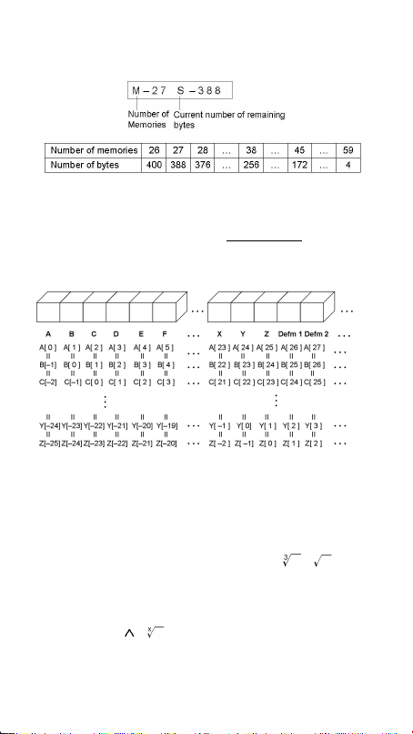
memories can be added in this way, giving you a maximum of 59 memories
(26 + 33).
Note: To restore the default memory configuration—26 memories—specify
Defm 0.
Expanded memories are named A [ 1 ] , A [ 2 ] etc and can be used in the
same way as standard memory variables. See Example 7.
Note: When using array variables, be careful to avoid overlap of memories.
The relation between memories is as follows:
Order of Operations
Each calculation is performed in the following order of precedence:
1. Functions inside parentheses, coordinate transformations, and Type B
functions, that is, those where you must press the function key before
entering the argument, for example, sin, cos, tan, sin-1, cos-1, tan-1, sinh,
cosh, tanh, sinh-1, cosh-1, tanh-1, log, ln, 10 X , e X, , , NEG,
NOT, X’( ), Y ’( ), MAX, MIN, SUM, SGN, AVG, ABS, INT, Frac, Plot.
2. Type A functions, that is, those where you enter the argument before
pressing the function key, for example, x 2, x 3, x-1, x!, º, r, g, %,
ENGSYM.
3. Exponentiation ( ),
4. Fractions
º΄ ΄΄
,
E-9
Page 10

5. Abbreviated multiplication format involving variables, π, RAND,
RANDI.
6. ( – )
7. Abbreviated multiplication format in front of Type B functions, ,
Alog2, etc.
8. nPr, nCr
9. × ,
10. +, –
11. Relational operators: = =, < , >, ≠, ≤ , ≥
12. AND, NAND (BaseN calculations only)
13. OR, XOR, XNOR (BaseN calculations only)
14. Conversion (A b/c d/e, F D, DMS)
When functions with the same priority are used in series, execution is
performed from right to left. For example:
e X ln120 → e X { ln (120 ) }
Otherwise, execution is from left to right.
Compound functions are executed from right to left.
Accuracy and Capacity
Output digits: Up to 10 digits
Calculating digits: Up to 24 digits
Where possible, every calculation is displayed in up to 10 digits, or as a
10-digit mantissa together with a 2-digit exponent up to 10
The arguments you input must be within the range of the associated function.
The following table sets out the allowable input ranges.
Functions Allowable Input range
sin x, cos x,
tan x
Deg : x < 4.5 × 10
Rad : x < 2.5 × 10 8πrad
Grad : x < 5 × 10
however, for tan x
Deg : x ≠ 90 (2n+1)
Rad : x ≠
π
(2n+1)
2
Grad : x ≠ 100 (2n+1)
(n is an integer)
–1
–1
sin
x, cos
x ≦ 1
x
10
10
deg
grad
±99
.
E-10
Page 11
–1
tan
x
sinh x, cosh x
tanh x
–1
sinh
x
–1
cosh
x
–1
tanh
x
x < 1 × 10
x ≦ 230.2585092
x < 1 × 10
x < 5 × 10
1 ≦ x < 5 × 10 99
x < 1
log x, ln x 1 × 10
10 x –1 × 10
e x –1 × 10
x 0 ≦ x < 1 × 10
2
x
-1
x
x
< 1 × 10
x
< 1 × 10
X ! 0 ≦ x ≦ 69, x is an integer.
P ( x, y )
y+x
R (r,θ) 0 ≦ r< 1 × 10
100
100
99
–99
≦ x < 1 × 10
100
< x < 100
100
< x ≦ 230.2585092
100
50
100
, x≠0
22
<1 × 10
100
100
Deg:│θ│<4.5 × 10 10 deg
Rad:│θ│<2.5 × 10 8πrad
Grad:│θ│<5 × 10
however, for tan x
Deg:│θ│≠90 (2n+1)
Rad:│θ│≠
π
(2n+1)
2
10
Grad:│θ│≠100 (2n+1)
(n is an integer)
DMS │D│, M, S < 1 × 10
100
0 ≦ M, S,
y > 0 : x≠0, -1 × 10
100
x
< 10
100
y = 0: x > 0
y < 0 : x = 2n+1, I/n, n is an integer.
(n≠0)
but -1 × 10
100
< log | y | <100
100
grad
100
,
<
log y
<
E-11
Page 12

nPr, nCr
STAT
0 ≦ r ≦ n, n < 10
| x | < 1×10
1 -VAR : n ≦ 30, 2 -VAR : n ≦ 30
FREQ. = n, 0 ≦ n < 10
in 1-VAR mode
σx,σ
y, x, y, a, b, r : n≠0
100
100
,| y | < 1×10
, n, r are integers.
100
100
: n is an integer
Sx, Sy :n≠0,1
BaseN
DEC : - 2147483648 ≦ x ≦ 2147483647
BIN :
1000000000000000000000000000000
0≦x ≦
1111111111111111111111111111111
1
( for negative )
0≦x≦
0111111111111111111111111111111
1
(for zero, positive)
OCT : 20000000000≦x≦37777777777
(for negative)
0 ≦x≦17777777777 (for zero or positive)
HEX : 80000000≦x≦FFFFFFFF
(for negative)
0≦x≦7FFFFFFF (for zero or positive)
Error Conditions
When an illegal calculation is attempted or a program you enter causes an
error, an error message briefly appears and then the cursor moves to the
location of the error. See Example 3.
The following conditions will result in an error:
Message Meaning
DOMAIN Er 1. You have specified an argument that is outside the
DIVIDE BY O You attempted to divide by 0.
OVERFLOW Er The result of a calculation exceeds the limits of the
SYNTAX Er 1. Input error.
allowable range.
2. FREQ ( in 1-VAR stats) < 0 or not an integer.
3. USL < LSL
calculator.
E-12
Page 13

2. An improper argument was used in a command or
function.
3. An END statement is missing from a program.
LENGTH Er An entry exceeds 84 digits after implied multiplication
with auto-correction.
OUT OF SPEC You input a negative CPU or CPL value, where
x–USL
=C
and
PU
σ3
LSL–x
=C
PL
σ3
NEST Er Subroutine nesting exceeds 3 levels.
GOTO Er There is no corresponding Lbl n for a GOTO n.
GOSUB Er 1. There is no corresponding PROG n for a GOSUB PROG
2. Attempt to jump to a program area in which there is no
EQN SAVE Er Attempt to save an equation to a program area that
EMPTY Er Attempt to run a program from an area without an
MEMORY Er 1. Memory expansion exceeds the steps remaining in the
2. Attempt to use a memory when no memory has been
n.
program stored.
already has a stored program.
equation or program.
program.
expanded.
DUPLICATE The label name is already in use.
LABEL
Press [ CL/
] to clear an error message.
ESC
Chapter 3 : Basic Calculations
Arithmetic Calculation
• For mixed arithmetic operations, multiplication and division have
priority over addition and subtraction. See Example 8.
• For negative values, press [ (–) ] before entering the value. See
Example 9.
• Results greater than 10
form. See Example 10.
Display Format
10
or less than 10-9 are displayed in exponential
E-13
Page 14
• A decimal format is selected by pressing [ 2nd ] [ FIX ] and selecting a
value from the menu (F0123456789). To set the displayed decimal
places to n, enter a value for n directly, or press the cursor keys until
the value is underlined and then press [ ]. (The default setting is
floating point notation (F) and its n value is •). See Example 11.
• Number display formats are selected by pressing [ 2nd ] [ SCI/ENG ]
and choosing a format from the menu. The items on the menu are FLO
(for floating point), SCI (for scientific), and ENG (for engineering). Press
[ ] or [ ] until the desired format is underlined, and then press
[ ]. See Example 12.
• You can enter a number in mantissa and exponent format using the
[ EXP ] key. See Example 13.
• This calculator also provides 11 symbols for input of values using
engineering notation. Press [ 2nd ] [ ENG SYM ] to display the symbols.
See Example 14.
The symbols are listed below:
Parentheses Calculations
• Operations inside parentheses are always executed first. Up to 13
levels of consecutive parentheses are allowed in a single calculation.
See Example 15.
• Closing parentheses that would ordinarily be entered immediately prior
to pressing [ ] may be omitted. See Example 16.
Percentage Calculations
[ 2nd ] [ % ] divides the number in the display by 100. You can use this
function to calculate percentages, mark-ups, discounts, and percentage
ratios. See Example 17.
Repeat Calculations
You can repeat the last operation you executed by pressing [ ]. Even if
a calculation concluded with the [ ] key, the result obtained can be
used in a further calculation. See Example 18.
Answer Function
E-14
Page 15

When you enter a numeric value or numeric expression and press [ ],
the result is stored in the Answer function, which you can then quickly recall.
See Example 19.
Note: The result is retained even if the power is turned off. It is also retained
if a subsequent calculation results in an error.
Chapter 4 : Common Math Calculations
Logarithm and Antilogarithm
You can calculate common and natural logarithms and antilogarithms using
[ log ], [ ln ], [ 2nd ] [ 10 x ], and [ 2nd ] [ e x ]. See Example 20.
Fraction Calculation
Fractions are displayed as follows:
5 ┘12 =
56 U 5 ┘12 =
• To enter a mixed number, enter the integer part, press [ A b/c ], enter
the numerator, press [ A b/c ], and enter the denominator. To enter an
improper fraction, enter the numerator, press [ A b/c ], and enter the
denominator. See Example 21.
• During a calculation involving fractions, a fraction is reduced to its
lowest terms where possible. This occurs when you press [ + ], [ – ],
[ × ], [ ] ) or [ ]. Pressing [ 2nd ] [ A b/c d/e ] converts a
mixed number to an improper fraction and vice versa. See Example
22.
• To convert a decimal to a fraction or vice versa, press [ 2nd ]
[ F D ] and [ ]. See Example 23.
• Calculations containing both fractions and decimals are calculated in
decimal format. See Example 24.
Converting Angular Units
You can specify an angular unit of degrees (DEG), radians (RAD), or grads
(GRAD). You can also convert a value expressed in one angular unit to its
corresponding value in another angular unit.
The relation between the anglular units is :
180° = π radians = 200 grads
E-15
Page 16

To change the angular unit setting to another setting, press
[ DRG ] repeatedly until the angular unit you want is indicated on the
display.
The conversion procedure follows (also see Example 25):
1. Change the angle units to the units you want to convert to.
2. Enter the value of the unit to convert.
3. Press [ 2nd ] [ DMS ] to display the menu. The units you can select are
°(degrees), ’ (minutes), ” (seconds), r (radians), g (gradians) orDMS
(Degrees-Minutes-Seconds).
4. Select the units you are converting from.
5. Press [ ] twice.
To convert an angle to DMS notation, selectDMS. An example of DMS
notation is 1° 30’ 0” (= 1 degrees, 30 minutes, 0 seconds). See Example
26.
To convert from DMS notation to decimal notation, select
°(degrees), ’(minutes), ”(seconds). See Example 27.
Trigonometric and Inverse Trigonometric functions
The calculator provides standard trigonometric functions and inverse
trigonometric functions: sin, cos, tan, sin-1, cos-1 and tan-1. See Example 28.
Note: Before undertaking a trigonometric or inverse trigonometric
calculation, make sure that the appropriate angular unit is set.
Hyperbolic and Inverse Hyperbolic functions
The [ 2nd ] [ HYP ] keys are used to initiate hyperbolic and inverse
hyperbolic calculations using sinh, cosh, tanh, sinh
Example 29.
Note: Before undertaking a hyperbolic or inverse hyperbolic calculation,
make sure that the appropriate angular unit is set.
-1
, cosh-1 and tanh-1. See
Coordinate Transformations
Press [ 2nd ] [ R P ] to display a menu to convert rectangular coordinates
to polar coordinates or vice versa. See Example 30.
Note: Before undertaking a coordinate transformation, make sure that the
appropriate angular unit is set.
Mathematical Functions
E-16
Page 17

Press [ MATH ] repeatedly to is display a list of mathematical functions and
their associated arguments. See Example 31. The functions available are:
! Calculate the factorial of a specified positive integer n , where
n≦69.
RAND Generate a random number between 0 and 1.
RANDI Generate a random integer between two specified integers, A
and B, where A ≦ random value≦ B.
RND Round off the result.
MAX Determine the maximum of given numbers. (Up to 10 numbers
can be specified.)
MIN Determine the minimum of given numbers. (Up to 10 numbers
can be specified.)
SUM Determine the sum of given numbers. (Up to 10 numbers can
be specified.)
AVG Determine the average of given numbers. (Up to 10 numbers
can be specified.)
Frac Determine the fractional part of a given number.
INT Determine the integer part of a given number.
SGN Indicate the sign of a given number: if the number is
negative, –1 is displayed; if zero, 0 is displayed; if positive, 1
is displayed.
ABS Display the absolute value of a given number.
nPr Calculate the number of possible permutations of n items taken
r at a time.
nCr Calculate the number of possible combinations of n items
taken r at a time.
Defm Memory expansion.
Other Functions ( x-1, , , ,x 2, x 3, ^ )
The calculator also provides reciprocal ( [ x -1] ), square root ( [ ] ), cube
root ( [ ] ), square ( [ x
exponentiation ( [ ^ ] ) functions. See Example 32.
2
] ), universal root ( [ ] ), cubic ( [ x 3 ] ) and
Unit Conversion
You can convert numbers from metric to imperial units and vice versa. See
Example 33. The procedure is:
E-17
Page 18

1. Enter the number you want to convert.
2. Press [ 2nd ] [ CONV ] to display the units menu. There are 7 menus,
covering distance, area, temperature, capacity, weight, energy, and
pressure.
3. Press [ ] or [ ] to scroll through the list of units until the
appropriate units menu is shown, then press [ ] .
4. Press [ ] or [ ] to convert the number to the highlighted unit.
Physics Constants
You can use the following physics constants in your calculations:
Symbol M eaning Valu e
c Speed of lig ht 299792458 m / s
g Acceleration of gravity 9.80665 m.s -2
G Gravitational constant 6.6725985 × 10
Vm Molar volume of ideal gas 0.0224141 m 3 mol -1
NA Avogadro’s number 6.022136736 × 10 23 mol -1
e Elementary charge 1.602177335 × 10
me Electron mass 9.109389754 × 10
mp Pro to n ma ss 1.67262311 × 10
h Planck ’s cons ta nt 6.62607554 × 10
k Boltzmann’s constant 1.38065812 × 10
IR Gas constant 8.3145107 J / mol • k
IF Fa raday co nstant 96485.30929 C / mol
mn Neutron constant 1.67492861 × 10
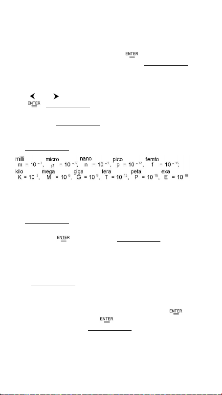
µ
Atomic mass constant 1.66054021 × 10
Dielectric permittivity 8.854187818 × 10
ε
0
µ
Magnetic permittivity 1.256637061 × 10 -6 N A -2
0
φ
Flux quantum 2.067834616 × 10
0
a 0 Boh r ra di us 5.291772492 × 10
µ
B Bohr magneton 9.274015431 × 10
µ
N Nuclear magneton 5.050786617 × 10
All physical constants in this manual are based on the 1986 CODATA
recommended values of the fundamental physical constants.
To insert a constant:
-11
m 3 kg -1 s -2
-12
-24
-19
-31
kg
-27
kg
-34
J.S
-23
J.K -1
-27
kg
-27
kg
F / m
-15
Wb
-11
J / T
-27
J / T
C
m
E-18
Page 19
1. Position your cursor where you want the constant inserted.
2. Press [ 2nd ] [ CONST ] to display the physics constants menu.
3. Scroll through the menu until the constant you want is underlined.
4. Press [ ]. (See Example 34.)
Multi-statement functions
Multi-statement functions are formed by connecting a number of individual
statements for sequential execution. You can use multi-statements in manual
calculations and in the program calculations.
When execution reaches the end of a statement that is followed by the
display result command symbol ( ), execution stops and the result up to
that point appears on the display. You can resume execution by pressing
[ ]. See Example 35.
Chapter 5 : Graphs
Built-in Function Graphs
You can produce graphs of the following functions: sin, cos, tan, sin -1, cos -1,
tan -1, sinh, cosh, tanh, sinh -1, cosh -1, tanh -1, , , x2, x3, log, ln, 10
x
, e x, x –1.
When you generate a built-in graph, any previously generated graph is
cleared. The display range is automatically set to the optimum. See Example
36.
User-generated Graphs
You can also specify your own single-variable functions to graph (for
example, y = x 3 + 3x 2 – 6x – 8). Unlike built-in functions (see above), you
must set the display range when creating a user generated graph.
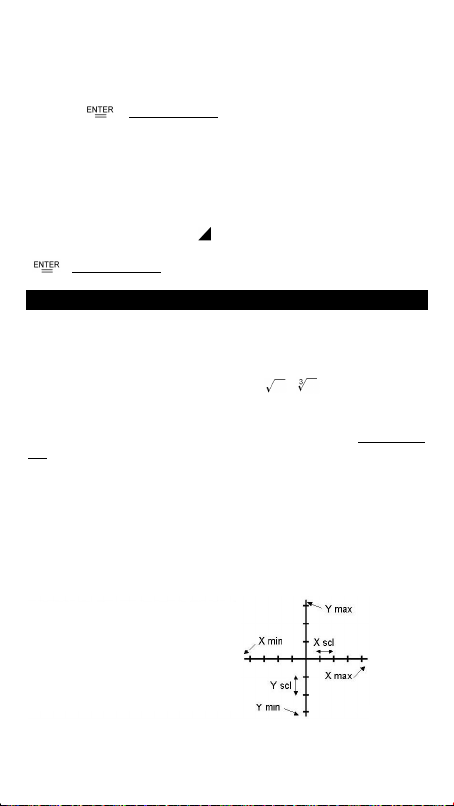
Press the [ Range ] key to access the
range parameters for each axis:
minimum value, maximum value, and
scale (that is, the distance between
the tick marks along an axis).
E-19
Page 20

After setting the range, press [ Graph ] and enter the expression to be
graphed. See Example 37.
Graph ↔ Text Display and Clearing a Graph
Press [ G T ] to switch between graph display and text display and vice
versa.
To clear the graph, please press [ 2nd ] [ CLS ].
Zoom Function
The zoom function lets you enlarge or reduce the graph. Press [ 2nd ]
[ Zoom x f ] to specify the factor for enlarging the graph, or press [ 2nd ]
[ Zoom x 1/f ] to specify the factor for reducing the graph. To return the
graph to its original size, press [ 2nd ] [ Zoom Org ]. See Example 37.
Superimposing Graphs
• A graph can be superimposed over one or more graphs. This makes it
easy to determine intersection points and solutions that satisfy all the
corresponding expressions. See Example 38.
• Be sure to input variable X in the expression for the graph you want to
superimpose over a built-in graph. If variable X is not included in the
second expression, the first graph is cleared before the second graph is
generated. See Example 39.
Trace Function
E-20
Page 21

This function lets you move a pointer around a graph by pressing [ ] and
[ ]. The x- and y-coordinates of the current pointer location are displayed
on the screen. This function is useful for determining the intersection of
superimposed graphs (by pressing [ 2nd ] [ X Y ]). See Example 40.
Note: Due to the limited resolution of the display, the position of the pointer
may be an approximation.
Scrolling Graphs
After generating a graph, you can scroll it on the display. Press [ ] [ ]
[ ] [ ] to scroll the graph left, right, up or down respectively. See
Example 41.
Plot and Line Function
The plot function is used to mark a point on the screen of a graph display.
The point can be moved left, right, up, or down using the cursor keys. The
coordinates of the point are displayed.
When the pointer is at the desired location, press [ 2nd ] [ PLOT ] to plot a
point. The point blinks at the plotted location.
Two points can be connected by a straight line by pressing [ 2nd ] [ LINE ].
See Example 42.
Chapter 6 : Statistical Calculations
The statistics menu has four options: 1-VAR (for analyzing data in a single
dataset), 2-VAR (for analyzing paired data from two datasets), REG (for
performing regression calculations), and D-CL (for clearing all datasets).
Single-Variable and Two-Variable Statistics
1. From the statistics menu, choose 1-VAR or 2-VAR and press [ ].
2. Press [ DATA ], select DATA-INPUT from the menu and press [ ].
3. Enter an x value and press [ ].
4. Enter the frequency ( FREQ ) of the x value (in 1-VAR mode) or the
corresponding y value ( in 2-VAR mode ) and press [ ].
5. To enter more data, repeat from step 3.
6. Press [ 2nd ] [ STATVAR ].
E-21
Page 22
7. Press [ ] [ ] [ ] or [ ] to scroll through the statistical
variables until you reach the variable you are interested in (see table
below).
Variable Meaning
n Number of x values or x–y pairs entered.
or Mean of the x values or y values.
Xmax or Ymax Maximum of the x values or y values.
Xmin or Ymin Minimum of the x values or y values.
Sx or Sy Sample standard deviation of the x values or y values.
σ
x orσy Population standard deviation of the x values or y
Σ
x or Σy Sum of all x values or y values.
Σ
x 2 or Σy 2 Sum of all x 2 values or y 2 values.
Σ
x y Sum of (x × y) for all x–y pairs.
CV x or CV y Coefficient of variation for all x values or y values.
R x or R y Range of the x values or y values.
8. To draw 1-VAR statistical graphs, press [ Graph ] on the STATVAR
menu. There are three types of graph in 1-VAR mode: N-DIST (Normal
distribution), HIST (Histogram), SPC (Statistical Process Control). Select
the desired graph type and press [ ]. If you do not set display
ranges, the graph will be produced with optimum ranges. To draw a
scatter graph based on 2-VAR datasets, press [ Graph ] on the
STATVAR menu.
9. To return to the STATVAR menu, press [ 2nd ] [ STATVAR ].
values.
Process Capability
(See Examples 43 and 44.)
1. Press [ DATA ], select LIMIT from the menu and press [ ].
2. Enter a lower spec. limit value ( X LSL or Y LSL ), then press [ ].
3. Enter a upper spec. limit value ( X USL or Y USL), then press [ ] .
4. Select DATA-INPUT mode and enter the datasets.
5. Press [ 2nd ] [ STATVAR ] and press [ ] [ ] [ ] [ ] to scroll
through the statistical results until you find the process capability
variable you are interested in (see table below).
Variable Meaning
Cax or Cay Capability accuracy of the x values or y values
E-22
Page 23
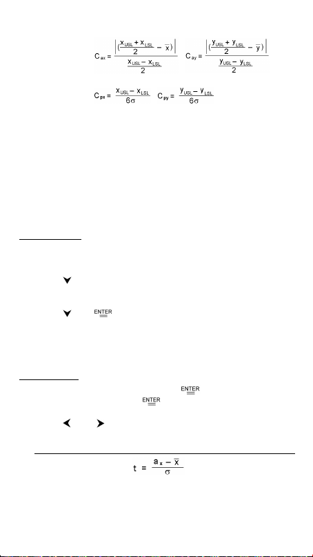
,
Cpx or Cpy Potential capability precision of the x values or y values,
,
Cpkx or Cpky Minimum (CPU, CPL) of the x values or y values, where
CPU is the upper spec. limit of capability precision and
CPL is lower spec. limit of capability precision.
C
pkx
C
pky
= Min (C
= Min (C
, C
PUX
, C
PUY
) = Cpx(1–Cax)
PLX
) = Cpy(1–Cay)
PLY
ppm Parts per million, Defection Per Million Opportunities.
Note: When calculating process capability in 2-VAR mode, the x n and y n
values are independent of each other.
Correcting Statistical Data
See Example 45.
1. Press [ DATA ].
2. To change the data, select DATA-INPUT. To change the upper or lower
spec. limit, select LIMIT. To change ax, select DISTR.
3. Press [ ] to scroll through the data until the entry you want to
change is displayed.
4. Enter the new data. The new data you enter overwrites the old entry.
5. Press [ ] or [ ] to save the change.
Note: The statistical data you enter is retained when you exit statistics mode.
To clear the data, select D-CL mode.
Probability Distribution (1-Var Data)
See Example 46.
1. Press [ DATA ] , select DISTR and press [ ].
2. Enter a a x value, then press [ ].
3. Press [ 2nd ] [ STATVAR ].
4. Press [ ] or [ ] to scroll through the statistical results until you find
the probability distribution variables you want (see table below).
Variable Meaning
t Test value
P(t) The cumulative fraction of the standard normal
distribution that is less than t.
E-23
Page 24
R(t) The cumulative fraction of the standard normal
Q(t) The cumulative fraction of the standard normal
distribution that lies between t and 0. R(t) = 1 – t.
distribution that is greater than t. Q(t) = | 0.5– t |.
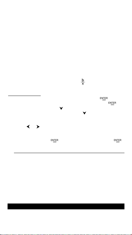
Regression Calculation
There are six regression options on the REG menu:
LIN Linear Regression y = a + b x
LOG Logarithmic Regression y = a + b lnx
e ^ Exponential Regression y = a • e bx
PWR Power Regression y = a • x b
INV Inverse Regression y = a +
QUAD Quadratic Regression y = a + b x + c x 2
See Example 47~48.
1. Select a regression option on the REG menu and press [ ] .
2. Press [ DATA ], select DATA-INPUT from the menu and press [ ].
3. Enter an x value and press [
4. Enter the corresponding y value and press [
5. To enter more data, repeat from step 3.
6. Press [ 2nd ] [ STATVAR ].
7. Press [ ] [ ] to scroll through the results until you find the
regression variables you are interested in (see table below).
8. To predict a value for x (or y) given a value for y (or x), select the x ’
(or y ’) variable, press [ ] , enter the given value, and press [ ]
again.
Variable Meaning
a Y-intercept of the regression equation.
b Slope of the regression equation.
r Correlation coefficient.
c Quadratic regression coefficient.
x ’ Predicted x value given a, b, and y values.
y ’ Predicted y value given a, b, and x values.
9. To draw the regression graph, press [ Graph ] on the STATVAR menu.
To return to the STATVAR menu, press [ 2nd ] [ STATVAR ].
].
].
Chapter 7 : BaseN Calculations
E-24
Page 25

You can enter numbers in base 2, base 8, base 10 or base 16. To set the
number base, press [ 2nd ] [ dhbo ], select an option from the menu and
press [ ]. An indicator shows the base you selected: d, h, b , or o. (The
default setting is d: decimal base). See Example 49.
The allowable digits in each base are:
Binary base (b): 0, 1
Octal base (o): 0, 1, 2, 3, 4, 5, 6, 7
Decimal base (d): 0, 1, 2, 3, 4, 5, 6, 7, 8, 9
Hexadecimal base (h): 0, 1, 2, 3, 4, 5, 6, 7, 8, 9, IA, IB, IC, ID, IE, IF
Note: To enter a number in a base other than the set base, append the
corresponding designator (d, h, b, o) to the number (as in h3).
Press [ ] to use the block function, which displays a result in octal or binary
base if it exceeds 8 digits. Up to 4 blocks can be displayed. See Example 50.
Negative Expressions
In binary, octal, and hexadecimal bases, negative numbers are expressed
as complements. The complement is the result of subtracting that number
from 10000000000 in that number’s base. You do this by pressing [ NEG ]
in a non-decimal base. See Example 51.
Basic Arithmetic Operations for Bases
You can add, subtract, multiply, and divide binary, octal, and hexadecimal
numbers. See Example 52.
Logical Operation
The following logical operations are available: logical products (AND),
negative logical (NAND), logical sums (OR), exclusive logical sums (XOR),
negation (NOT), and negation of exclusive logical sums (XNOR). See Example
53.
Chapter 8 : Programming
The options on the program menu are: NEW (for creating a new program), RUN
(for executing a program), EDIT (for editing a program), DEL (for deleting a
program), TRACE (for tracing a program), and EXIT (for exiting program mode).
E-25
Page 26

Before Using the Program Area
Number of Remaining Steps: The program capacity is 400 steps. The
number of steps indicates the amount of storage space available for
programs, and it will decrease as programs are input. The number of
remaining steps will also decrease when steps are converted to memories.
See Array Variables above.
Program Type: You must specify in each program the calculation mode that
the calculator should enter when executing the program. To perform binary,
octal or hexadecimal calculations or conversions, choose BaseN; otherwise
choose MAIN.
Program Area: There are 10 program areas for storing programs (P0–P9 ). If
an area has a program stored in it, its number is displayed as a subscript (as
in P1).
Program Control Instructions
The calculator’s programming language is similar to many programming
languages, such as BASIC and C. You can access most of the programming
commands from the program control instructions. You display these
instructions by pressing [ 2nd ] [ INST ].
Clear screen command
CLS
Clear the display on the screen.
⇒
Input and output commands
E-26
Page 27

INPUT memory variable
Makes the program pause for data input. memory variable = _
⇒
appears on the display. Enter a value and press [ ]. The value is
assigned to the specified variable, and the program resumes execution.
To input more than one memory variable, separate them with a
semicolon (;).
PRINT “ text ” , memory variable
Print the text specified inside the double quotation marks and the
⇒
value of the specified memory variable.
Conditional branching
IF
( condition
) THEN {
statement }
IF the condition is true, THEN statement is executed.
⇒
IF (
condition
) THEN {
statement
}; ELSE {
statement
}
IF the condition is true, the specified THEN statement is executed,
⇒
otherwise the ELSE statement is executed.
Jump commands
Lbl n
An Lbl n command marks a destination point for a GOTO n jump
⇒
command. Each label name (Lbl) must be unique (that is, not repeated in
the same program area). The label suffix n must be an integer from 0 to
9.
GOTO n
When program execution encounters a GOTO n statement, execution
⇒
jumps to Lbl n (where n is the same value as t he n in the GOTO n
statement).
Mainroutine and Subroutine
GOSUB PROG n ;
You can jump between program areas, so that the resulting execution
⇒
is made up of code from different program areas. The program from
which other program areas are jumped to is the mainroutine, and an
area jumped to is a subroutine. To cause a jump to a subroutine, enter
PROG n where n is the number of the destination program area.
Note: The GOTO n command does not allow jumps between program
areas. A GOTO n command only jumps to the corresponding label (Lbl)
within the same program area.
End
E-27
Page 28

Each program needs an END command to mark the end of the
⇒
program. This is displayed automatically when you create a new
program.
Increment and decrement
Post-fixed: Memory variable + + or Memory variable – –
Pre-fixed: + + Memory variable or – – Memory variable
A memory variable is decreased or increased by one. For standard
⇒
memory variables, the + + ( Increment ) and – – ( Decrement ) operators
can be either post-fixed or pre-fixed. For array variables, the operators
must be pre-fixed.
With pre-fixed operators, the memory variable is computed before the
expression is evaluated; with post-fixed operators, the memory variable
is computed after the expression is evaluated.
For loop
FOR (
start condition; continue condition; re-evaluation ) { statements }
A FOR loop is useful for repeating a set of similar actions while a
⇒
specified counter is between certain values.
For example:
FOR
( A = 1 ; A ≤ 4 ; A + + )
×
A ; PRINT ” ANS = ” , C }
{ C = 3
END
Result : ANS = 3, ANS = 6, ANS = 9, ANS = 12
⇒
The processing in this example is:
1. FOR A = 1: This initializes the value of A to 1. Since A = 1 is consistent
with A
≤
2. Now A = 2. This is consistent with A ≤ 4, so the statements are
3. When A = 5, it is no longer true that A ≤ 4, so statements are not
Sleep command
Swap command
4, the statements are executed and A is incremented by 1.
executed and A is again incremented by 1. And so on.
executed. The program then moves on to the next block of code.
SLEEP (
time
)
A SLEEP command suspends program execution for a specified time
⇒
(up to a maximum of 105 seconds). This is useful for displaying
intermediate results before resuming execution.
SWAP (
memory variable A, memor y variable B
)
E-28
Page 29
The SWAP command swaps the contents in two memory variables.
⇒
Relational Operators
The relational operators that can be used in FOR loops and conditional
branching are:
= = (equal to), < (less than), > (greater than), ≠ (not equal to), ≤ (less
than or equal to), ≥ (greater than or equal to).
Creating a New Program
1. Select NEW from the program menu and press [ ].
2. Select the calculation mode you want the program to run in and press
[ ].
3. Select one of the ten program areas (P0123456789) and press [ ].
4. Enter your program’s commands.
• You can enter the calculator’s regular functions as commands.
• To enter a program control instruction, press [ 2nd ] [ INST ] and
make your selection.
• To enter a space, press [ ALPHA ] [ SPC ].
5. A semicolon (;) indicates the end of a command. To enter more than
one command on a command line, separate them with a semicolon. For
example:
Line 1:
INPUT
You can also place each command or group of commands on a
separate line, as follows. In this case, a trailing semicolon can be
omitted.
Line 1:
Line 2:
A ; C = 0.5 × A ;
INPUT
A ; C = 0.5 × A [ ]
PRINT
” C = ” , C ; END
PRINT
” C = ” , C ;
END
Executing a Program
1. When you finish entering or editing a program, press [ CL/
to the program menu, select RUN and press [ ]. (Or you can press
[ PROG ] in MAIN mode.)
2. Select the relevant program area and press [ ] to begin executing
the program.
3. To re-execute the program, press [ ] while the program’s final
result is on the display.
4. To abort the execution of a program, press [ CL/
appears asking you to confirm that you want to stop the execution.
STOP : N Y
Press [ ] to move the cursor to Y and then press [ ].
ESC
] to return
ESC
]. A message
E-29
Page 30

Debugging a Program
A program might generate an error message or unexpected results when it
is executed. This indicates that there is an error in the program that needs to
be corrected.
• Error messages appear for approximately 5 seconds, and then the
cursor blinks at the location of the error.
• To correct an error, select EDIT from the program menu.
• You also can select TRACE from the program menu. The program is
then checked step-by-step and a message alerts you to any errors.
Using the Graph Function in Programs
Using the graph function within programs enables you to graphically
illustrate long or complex equations and to overwrite graphs repeatedly. All
graph commands (except trace and zoom) can be included in programs.
Range values can also be specified in the program.
Note that values in some graph commands must be separated by commas
(,) as follows:
• Range ( Xmin, Xmax, Xscl, Ymin, Ymax, Yscl )
• Factor ( Xfact, Yfact )
• Plot ( X point, Y point )
Display Result Command
You can put in a program if you want to be able to see the value of a
variable at that particular stage in program execution.
For example:
Line 1:
INPUT
Line 2: C = 13 × A ; -------Stop at this point
Line 3: D = 51 / ( A × B )
Line 4:
1. Execution is interrupted at the point where you placed .
2. At this time, you can press [ 2nd ] [ RCL ] to view the value of the
3. To resume program execution, press [ ].
A ; B = ln ( A + 100 )
PRINT
” D = ”, D ; END
corresponding memory variable (C in the above example).
Deleting a Program
1. Select DEL from the program menu and press [ ].
2. To erase a single program, select ONE, the program area you want to
erase, and then press [ ]
E-30
Page 31

3. To erase all the programs, select ALL.
4. A message appears asking you to confirm that you want to delete the
program(s).
Press [ ] to move the cursor to Y and then press [ ].
5. To exit DEL mode, select EXIT from the program menu.
Program Examples
See Examples 54 to 63.
Example 1
Change 123 × 45 to 123 × 475
123 [ × ] 45 [ ]
[ ] [ ] [ ] [ DEL ]
[ 2nd ] [ ]
[ ] [ ] 7 [ ]
Example 2
After executing 1 + 2, 3 + 4, 5 + 6, recall each expression
1 [ + ] 2 [ ] 3 [ + ] 4
[ ] 5 [ + ] 6 [ ]
E-31
Page 32

[ ]
[ ]
[ ]
Example 3
Enter 14 0 × 2.3 and then correct it to 14 10 × 2.3
14 [ ] 0 [ × ] 2.3 [ ]
(after 5 Seconds )
[ ] 1 [ ]
Example 4
[ ( 3 × 5 ) + ( 56 7 ) – ( 74 – 8 × 7 ) ] = 5
3 [ × ] 5 [ M+ ]
E-32
Page 33

56 [ ] 7 [ M+ ]
[ MRC ] [ ]
74 [ – ] 8 [ × ] 7 [ 2nd ] [ M– ]
[ MRC ] [ ]
[ MRC ] [ MRC ] [
CL
/
]
ESC
Example 5
(1) Assign 30 into variable A
[ 2nd ] [ CL-VAR ] 30 [ SAVE ]
[ A ] [ ]
0 (2) Multiply variable A by 5 and assign the result to variable B
5 [ × ] [ 2nd ] [ RCL ]
[ ] [ ]
E-33
Page 34

[ SAVE ] [ B ] [ ]
1 (3) Add 3 to variable B
[ ALPHA ] [ B ]
[ + ] 3 [ ]
2 (4) Clear all variables
[ 2nd ] [ CL-VAR ] [ 2nd ]
[ RCL ]
Example 6
(1) Set PROG 1 = cos (3A) + sin (5B), where A = 0, B = 0
[ cos ] 3 [ ALPHA ] [ A ] [ ]
[ + ] [ sin ] 5 [ ALPHA ] [ B ]
[ ]
[ SAVE ] [ PROG ] 1
[ ]
3 (2) Set A = 20,B = 18, get PROG 1 = cos (3A) + sin (5B) = 1.5
E-34
Page 35

[ PROG ] 1 [ ] [
CL
[
/
] 20
ESC
]
[ ] [
CL
/
] 18
ESC
[ ]
Example 7
(1) Expand the number of memories from 26 to 28
[ MATH ] [ MATH ] [ MATH ]
[ MATH ] [
[ ] 2
[ ]
4 (2) Assign 66 to variable A [ 27 ]
66 [ SAVE ] [ A ] [ ALPHA ]
[ [ ] ] 27 [ ]
]
E-35
Page 36

5 (3) Recall variable A [ 27 ]
[ ALPHA ] [ A ] [ ALPHA ] [ [ ] ]
27 [ ]
6 (4) Return memory variables to the default configuration
[ MATH ] [ MATH ] [ MATH ]
[ MATH ] [ ]
[
] 0 [ ]
Example 8
7 + 10 × 8 2 = 47
7 [ + ] 10 [ × ] 8 [ ] 2
[ ]
Example 9
– 3.5 + 8 4 = –1.5
[ ( – ) ] 3.5 [ + ] 8 [ ] 4
[ ]
Example 10
12369 × 7532 × 74103 = 6903680613000
E-36
Page 37

12369 [ × ] 7532 [ × ] 74103
[ ]
Example 11
6 7 = 0.857142857
6 [ ] 7 [ ]
[ 2nd ] [ FIX ] [ ] [ ]
[ ]
[ ]
[ 2nd ] [ FIX ] 4
[ 2nd ] [ FIX ] [ • ]
Example 12
1 6000 = 0.0001666...
1 [ ] 6000 [ ]
E-37
Page 38

[ 2nd ] [ SCI / ENG ] [ ]
[ ]
[ 2nd ] [ SCI / ENG ] [ ]
[ ]
[ 2nd ] [ SCI / ENG ] [ ]
]
[
Example 13
0.0015 = 1.5 × 10
1.5 [ EXP ] [ (–) ] 3 [ ]
– 3
Example 14
20 G byte + 0.15 K byte = 2.000000015 × 10 10 byte
E-38
Page 39

20 [ 2nd ] [ ENG SYM ] [ ]
[ ]
[ ] [ + ] 0.15 [ 2nd ]
[ ENG SYM ]
[ ] [ ]
Example 15
( 5 – 2 × 1.5 ) × 3 = 6
[ ( ) ] 5 [ – ] 2 [ × ] 1.5 [ ]
[ × ] 3 [ ]
Example 16
2 × { 7 + 6 × ( 5 + 4 ) } = 122
2 [ × ] [ ( ) ] 7 [ + ] 6 [ × ]
[ ( ) ] 5 [ + ] 4 [
]
Example 17
120 × 30 % = 36
120 [ × ] 30 [ 2nd ] [ % ]
[ ]
7 88 55% = 160
E-39
Page 40

88 [ ] 55 [ 2nd ] [ % ]
[ ]
Example 18
3 × 3 × 3 × 3 = 81
3 [ × ] 3 [ ]
[ × ] 3 [ ]
[ ]
8 Calculate 6 after calculating 3 × 4 = 12
3 [ × ] 4 [ ]
[ ] 6 [ ]
Example 19
123 + 456 = 579 789 – 579 = 210
123 [ + ] 456 [ ]
E-40
Page 41

789 [ – ] [ 2nd ] [ ANS ]
[ ]
Example 20
ln7 + log100 = 3.945910149
[ ln ] 7 [ ] [ + ] [ log ] 100
[ ]
9 10 2 = 100
[ 2nd ] [ 10 x ] 2 [ ]
–5
10 e
= 0.006737947
[ 2nd ] [ e x ] [ ( – ) ] 5
[ ]
Example 21
7 [ A b/c ] 2 [ A b/c ] 3 [ + ] 14
[ A b/c ] 5 [ A b/c ] 7 [ ]
Example 22
E-41
Page 42

4 [ A b/c ] 2 [ A b/c ] 4
[ ]
[ 2nd ] [ A b/
[ ]
[ 2nd ] [A b/
d
c
d
/e ] [ ]
c
/e ]
Example 23
4 [ A b/c ] 1 [ A b/c ] 2 [ 2nd ]
[ F
D ] [
]
Example 24
8 [ A b/c ] 4 [ A b/c ] 5 [ + ]
3.75 [ ]
Example 25
2 rad. = 360 deg.
[ DRG ]
E-42
Page 43

[ ] 2 [ 2nd ] [ ]
[ 2nd ] [ DMS ] [ ] [ ]
[ ]
[ ] [ ]
Example 26
1.5 = 1O 30 I 0 II ( DMS )
1.5 [ 2nd ] [ DMS ] [ ]
[ ] [ ]
Example 27
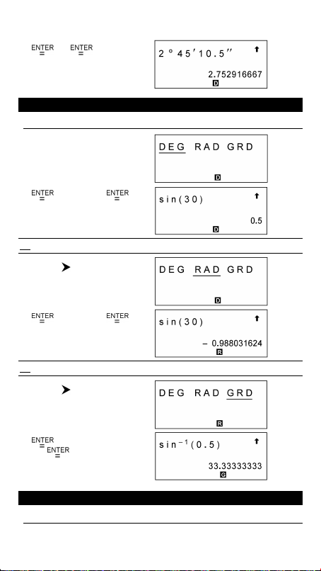
2 0 45 I 10.5
2 [ 2nd ] [ DMS ]
[ ] 45 [ 2nd ] [ DMS ]
[ ]
[ ] 10.5 [ 2nd ] [ DMS ]
[ ] [ ]
I I
= 2.752916667
E-43
Page 44
[ ] [ ]
Example 28
sin30 Deg. = 0.5
[ DRG ]
[ ] [ sin ] 30 [ ]
11 sin30 Rad. = – 0.988031624
[ DRG ] [ ]
[ ] [ sin ] 30 [ ]
12 sin –1 0.5 = 33.33333333 Grad.
[ DRG ] [ ]
[ ] [ 2nd ] [ sin –1 ]
0.5 [ ]
Example 29
cosh1.5+2 = 4.352409615
E-44
Page 45

[ 2nd ] [ HYP ] [ cos ] 1.5
[ ] [ + ] 2 [ ]
13 sinh –1 7 = 2.644120761
[ 2nd ] [ HYP ] [ 2nd ] [ sin
–1
]
7 [ ]
Example 30
If x = 5 and y = 30, what are r and ? Ans : r = 30.41381265, =
80.53767779 o
[ 2nd ] [ R P ]
[
[ ]
] 5 [ ALPHA ] [
] 30
[ 2nd ] [ R P ] [ ]
[ ] 5 [ ALPHA ] [ ] 30
[ ]
14 If r = 25 and = 56 o what are x and y? Ans : x = 13.97982259, y =
20.7259393 1
E-45
Page 46

[ 2nd ] [ R P ] [ ]
[ ] 25 [ ALPHA ] [ ]
56 [ ]
[ 2nd ] [ R P ] [ ] [ ]
[
56 [
] 25 [ ALPHA ] [
]
]
Example 31
5 ! = 120
5 [ MATH ]
] [ ]
[
15 Generate a random number between 0 and 1
[ MATH ] [ ]
[ ] [ ]
E-46
Page 47

16 Generate a random integer between 7 and 9
[ MATH ] [ ]
[ ] 7 [ ALPHA ] [ ]
9 [ ]
17 RND ( sin 45 Deg. ) = 0.71 ( FIX = 2 )
[ MATH ] [ ] [ ]
[ ] [ sin ] 45 [ 2nd ]
[ FIX ] [ ] [ ] [ ]
[ ] [ ]
18 MAX ( sin 30 Deg. , sin 90 Deg. ) = MAX ( 0.5, 1 ) = 1
[ MATH ] [ MATH ]
[ ] [ sin ] 30
[ ] [ ALPHA ] [ ] [ sin ] 90
[ ]
19 MIN ( sin 30 Deg., sin 90 Deg. ) = MIN ( 0.5, 1 ) = 0.5
E-47
Page 48

[ MATH ] [ MATH ] [ ]
[ ] [ sin ] 30
[ ] [ ALPHA ] [ ] [ sin ] 90
[ ]
20 SUM (13, 15, 23 ) = 51
[ MATH ] [ MATH ] [ ]
[ ] 13 [ ALPHA ] [ ]
15 [ ALPHA ] [ ] 23
[ ]
21 AVG (13, 15, 23 ) = 17
[ MATH ] [ MATH ] [ ]
[ ]
[ ] 13 [ ALPHA ] [ ]
15 [ ALPHA ] [ ] 23
[ ]
22 Frac (10 8 ) = Frac ( 1.25 ) = 0.25
[ MATH ] [ MATH ] [ MATH ]
E-48
Page 49

[ ] 10 [ ] 8 [ ]
23 INT (10 8 ) = INT ( 1.25 ) = 1
[ MATH ] [ MATH ] [ MATH ]
[ ]
[ ] 10 [ ] 8 [ ]
24 SGN ( log 0.01 ) = SGN ( – 2 ) = – 1
[ MATH ] [ MATH ] [ MATH ]
[ ]
[ ] [ log ] 0.01
[ ]
25 ABS ( log 0.01) = ABS ( – 2 ) = 2
[ MATH ] [ MATH ] [ MATH ]
[ ] [ ]
[ ] [ log ] 0.01
[ ]
E-49
Page 50

26 7 ! [ ( 7 – 4 ) ! ] = 840
7 [ MATH ] [ MATH ] [ MATH ]
[ MATH ]
[ ] 4 [ ]
27 7 ! [ ( 7 – 4 ) ! × 4 ] = 35
7 [ MATH ] [ MATH ] [ MATH ]
[ MATH ] [
[ ] 4 [ ]
]
Example 32
1.25 [ 2nd ] [ X –1 ] [ ]
28
2 [ X 2 ] [ + ] [ ] 4 [ + ] 21
[ ] [ + ] [ 2nd ] [ ] 27
[ ]
29
E-50
Page 51

4 [ 2nd ] [ ] 81
[ ]
30 7 4 = 2401
7 [ 2nd ] [ ^ ] 4 [
]
Example 33
1 yd 2 = 9 ft 2 = 0.000000836 km 2
1 [ 2nd ] [ CONV ] [ 2nd ]
[ CONV ] [ ]
[ ]
[ ]
[ ] [ ]
Example 34
3 × G = 2.00177955 × 10
–10
E-51
Page 52

3 [ × ] [ 2nd ] [ CONST ]
[ ] [ ]
[ ] [ ]
Example 35
Apply the multi-statement function to the following two statements:
( E=15 )
15 [ SAVE ] [ E ] [ ]
[ ALPHA ] [ E ] [ × ] 13
[ ALPHA ] [ ]180 [ ]
[ ALPHA ] [ E ] [ ]
[ ]
[ ]
Example 36
Graph Y = e X
E-52
Page 53

[ Graph ] [ 2nd ] [ e x ]
[ ]
Example 37
(1) Range : X min = – 180, X max = 180, X scl = 90, Y min = – 1.25, Y
max = 1.25, Y scl = 0.5, Graph Y = sin (2 x)
[ Range ] [ ( – ) ] 180
[ ] 180 [ ] 90 [ ]
[ (–) ] 1.25 [ ] 1.25 [ ]
0.5
[ ] [ 2nd ] [ Factor ] 2
[ ] 2
[ ] [ Graph ] [ sin ] 2
[ ALPHA ] [ X ]
[ ]
E-53
Page 54

[ G T ]
[ G T ]
31 (2) Zoom in and zoom out on Y = sin (2x)
[ 2nd ] [ Zoom x f ]
[ 2nd ] [ Zoom x f ]
[ 2nd ] [ Zoom Org ]
[ 2nd ] [ Zoom x 1 / f ]
[ 2nd ] [ Zoom x 1 / f ]
Example 38
Superimpose the graph of Y = – X + 2 over the graph of Y = X 3 + 3 X
2
– 6 X – 8
E-54
Page 55

[ Range ] [ (–) ] 8 [ ] 8
[ ] 2 [ ] [ (–) ] 15 [ ]
15 [ ] 5
[ ] [ Graph ] [ ALPHA ]
[ X ] [ 2nd ] [ x 3 ] [ + ] 3
[ ALPHA ] [ X ] [ x 2 ] [ – ] 6
[ ALPHA ] [ X ] [ – ] 8
[ ]
[ Graph ] [ (–) ] [ ALPHA ] [ X ]
[ + ] 2
[ ]
Example 39
Superimpose the graph of Y = cos (X) over the graph of Y = sin ( x )
[ Graph ] [ sin ] [ ]
[ Graph ] [ cos ] [ ALPHA ] [ X ]
[ ]
Example 40
Use Trace function to analyze the graph Y = cos ( x )
E-55
Page 56

[ Graph ] [ cos ] [ ]
[ Trace ]
[ ] [ ] [ ]
[ 2nd ] [ X Y ]
Example 41
Draw and scroll the graph for Y = cos ( x )
[ Graph ] [ cos ] [
[
]
[ ] [ ]
[ ] [ ] [ ] [ ]
[ ]
]
Example 42
Place points at ( 5 , 5 ), ( 5 , 10 ), ( 15 , 15 ) and ( 18, 15 ), and then
use the Line function to connect the points.
E-56
Page 57

[ Range ] 0 [ ] 35 [ ] 5
[ ] 0 [ ] 23 [ ] 5
[ ] [ 2nd ] [ PLOT ] 5
[ ALPHA ] [ ] 5
[ ]
[ 2nd ] [ X Y ]
[ 2nd ] [ X Y ] [ 2nd ]
[ PLOT ] 5 [ ALPHA ] [ ] 10
[ ]
[ 2nd ] [ LINE ] [ ]
[ 2nd ] [ PLOT ] 15 [ ALPHA ]
[ ] 15 [ ] [ 2nd ]
[ LINE ] [ ]
[ 2nd ] [ PLOT ] 18 [ ALPHA ]
[ ] 15 [ ] [ ]
[ ] [ ] [ ] [ ]
[ ] [ ] [ ]
[ 2nd ] [ LINE ] [ ]
E-57
Page 58

Example 43
Enter the data: X
= 9, X 3 = 12, FREQ 3 = 7, then find = 7.5, Sx = 3.745585637,
Cax = 0 , and Cpx = 0.503655401
[ MODE ] 1
[ ] [ DATA ] [ ]
[ ] 2
LSL
= 2, X
= 13, X 1 = 3, FREQ 1 = 2, X 2 = 5 , FREQ 2
USL
[ ] 13 [
]
[ DATA ]
[ ] 3
[ ] 2
[ ] 5 [ ] 9 [ ] 12
[ ] 7
E-58
Page 59

[ 2nd ] [ STATVAR ]
[ ]
[ ]
[ Graph ] [ ]
[ ]
[ 2nd ] [ STATVAR ] [ ]
[
] [ ] [ ]
[ ]
[ Graph ]
[ ]
E-59
Page 60
[ 2nd ] [ STATVAR ] [ Graph ]
[ ] [ ]
[ ]
Example 44
Enter the data : X
= 5 , Y 2 = 7, X 3 = 7, Y 3 = 6, then find = 5, Sx = 2, Cax =
2
0, Cay = 0.111111111
[ MODE ] 1 [ ]
[ ] [ DATA ] [ ]
[ ] 2 [ ] 8 [ ] 3
[ ] 9 [ ]
[ DATA ]
[ ] 3 [ ] 4 [ ] 5
[ ] 7 [ ] 7 [ ] 6
= 2, X
LSL
= 8, Y
USL
= 3, Y
LSL
USL
= 9, X 1 = 3, Y 1 = 4, X
E-60
Page 61

[ 2nd ] [ STATVAR ] [ ]
[ ]
[ ] [ ] [ ] [ ]
] [ ] [ ] [ ]
[
[ ]
[ Graph ]
Example 45
In the data in Example 44, change Y 1 = 4 to Y 1 = 9 and X 2 = 5 to X
= 8, then find Sx = 2.645751311
2
[ DATA ]
[ ] [ ] 9
[ ] 8
E-61
Page 62
[ 2nd ] [ STATVAR ] [ ]
[ ]
Example 46
Enter the data : a x = 2, X 1 = 3, FREQ 1 = 2, X 2 = 5 , FREQ 2 = 9, X 3
= 12, FREQ3 = 7, then find t = –1.510966203, P( t ) = 0.0654,
Q( t ) = 0.4346, R ( t ) =0.9346
[ MODE ] 1
[ ] [ DATA ] [ ]
[ ]
] 2 [ ]
[
[ DATA ] [ ] 3 [ ] 2
[ ] 5 [ ] 9 [ ] 12
[ ] 7
[ 2nd ] [ STATVAR ] [ ]
[ ]
E-62
Page 63

[ ]
[ ]
Example 47
Given the following data, use linear regression to estimate x ’ =? for y
=573 and y ’= ? for x = 19
X 15 17 21 28
Y 451 475 525 678
[ MODE ] 1 [ ]
[ ]
[ ] [ DATA ]
[ ] 15 [ ] 451 [ ]
17 [ ] 475 [ ] 21 [ ]
525 [ ] 28 [ ] 678
E-63
Page 64

[ 2 nd ] [ STATVAR ] [ Graph ]
[ 2nd ] [ STATVAR ] [ ]
[ ] [ ]
[ ] 573 [
[ 2nd ] [ STATVAR ] [ ]
[
] [ ] [ ]
] 19 [ ]
[
]
Example 48
Given the following data, use quadratic regression to estimate y ’ = ? for
x = 58 and x ’ =? for y =143
X 57 61 67
Y 101 117 155
[ MODE ] 1 [ ]
E-64
Page 65

[ ] [ ] [ ]
[ ] [ DATA ]
[ ] 57 [ ] 101 [ ]
61 [ ] 117 [ ] 67
[ ]155
[ 2nd ] [ STATVAR ] [ Graph ]
[ 2 nd ] [ STATVAR ] [ ]
[ ] [ ]
[ ] 143 [ ]
[ ]
[ 2nd ] [ STATVAR ] [ ]
[ ] [ ] [ ]
E-65
Page 66
[ ] 58 [ ]
Example 49
31 10 = 1F16 = 11111 2 = 37 8
[ MODE ] 2
31 [ ]
[ dhbo ]
[ ]
[ ]
[ ]
Example 50
4777 10 = 1001010101001 2
E-66
Page 67

[ MODE ] 2 [ dhbo ] [ ]
[ ]
[ ] [ dhbo ] [ ] [ ]
[ ] 4777 [ ]
[ ]
[ ]
[ ]
Example 51
What is the negative of 3A 16? Ans : FFFFFFC6
[ MODE ] 2 [ dhbo ] [ ]
[ ] [ NEG ] 3 [ /A ]
[ ]
Example 52
1234
+ 1EF 16 24 8 = 2352 8 = 1258 10
10
E-67
Page 68

[ MODE ] 2 [ dhbo ] [ ]
[ ] [ dhbo ] [ ] [ ]
[ ] 1234 [ + ]
[ dhbo ] [ ] [ ] [ ]
[ ] 1[ IE ] [ IF ] [ ]
[ dhbo ] [ ] [ ]
[ ] 24
[ ]
[ dhbo ] [ ] [ ] [ ]
Example 53
E-68
Page 69

1010 2 AND ( A 16 OR 7 16 ) = 1010 2 = 10 10
[ MODE ] 2 [ dhbo ] [ ]
[ ]
[ ] [ dhbo ] [ ] [ ]
[ ] [ ]
[ ] 1010 [ AND ] [ ( ) ]
[ dhbo ] [ ] [ ] [ ]
[ ] [ /A ] [ OR ] [ dhbo ]
[ ] [ ] [ ]
[ ] 7 [ ]
[ dhbo ] [ ] [ ]
Example 54
Create a program to perform arithmetic calculation with complex
numbers
Z 1 = A + B i, Z 2 = C + D i
• Sum : Z 1 + Z 2 = ( A + B ) + ( C + D ) i
• Difference : Z 1 – Z 2 = ( A – B ) + ( C – D ) i
• Product : Z 1 × Z 2 = E + F i = ( AC – BD ) + ( AD + BC ) i
E-69
Page 70

• Quotient : Z 1Z 2 = E + F i =
RUN
When the message “1 : + ”, “ 2 : – ”, “ 3 : × ”, “ 4 : / ” appears on the
display, you can input a value for “ O ” that corresponds to
the type of operation you want to performed, as follows:
1 for Z 1 + Z 2 2 for Z 1 – Z 2
3 for Z 1 × Z 2 4 for Z 1 Z 2
(1)
E-70
Page 71

[ ] ( 5 Seconds )
[ ] 1
[ ] 17 [ ]
5 [ ] [ ( – ) ] 3 [ ]
14
[ ]
(2)
[ ] ( 5 Seconds )
[ ] 2
E-71
Page 72

[ ] 10 [ ]
13 [ ] 6 [ ] 17
[ ]
(3)
[ ] ( 5 Seconds )
[ ] 3
[ ] 2 [ ]
[ ( – ) ] 5 [ ] 11
[ ] 17
[ ]
(4)
E-72
Page 73

[ ] ( 5 Seconds )
[ ] 4
[ ] 6 [ ] 5
[ ] [ ( – ) ] 3 [ ] 4
[ ]
Example 55
Create a program to determine solutions to the quadratic equation A X 2
+ B X + C = 0, D = B
1) D > 0 ,
2) D = 0
3) D < 0 ,
2 –
4AC
,
,
E-73
Page 74

RUN
(1) 2 X 2 – 7 X + 5 = 0 X 1 = 2.5 , X 2 = 1
[ ]
2 [ ] [ ( – ) ] ] 7
[ ] 5
[ ]
(2) 25 X 2 – 70 X + 49 = 0 X = 1.4
[ ]
25 [ ] [ ( – ) ]
70[ ] 49
E-74
Page 75

[ ]
(3) X 2 + 2 X + 5 = 0 X 1 = – 1 + 2 i , X 2 = – 1 – 2 i
[ ]
1 [ ] 2 [ ] 5
[ ]
[ ] [ ] [ ] [ ]
[ ] [ ] [ ] [ ]
] [ ] [ ] [ ]
[
[
] [ ] [ ][ ]
Example 56
Create a program to generate a common difference sequence ( A : First
item, D : common difference, N : number )
Sum : S ( N ) = A+(A+D)+(A+2D)+(A+3D)+...
=
Nth item : A ( N ) = A + ( N – 1 ) D
E-75
Page 76

RUN
When the message “ 1: A(N), 2 :S(N) ” appears on the display, you can
input a “ P ” value to specify the type of operation to be
performed:
1 for A(N) 2 for S(N)
32 (1) A = 3 , D = 2, N = 4 A(N) = A (4) = 9
[ ] ( 5 Seconds )
1 [ ] 3 [ ]
2 [ ] 4
[ ]
E-76
Page 77
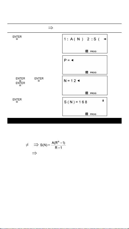
(2) A = 3 , D = 2, N = 12 S (N) = S (12) = 168
[ ] ( 5 Seconds )
2 [ ] 3 [ ]
2 [ ] 12
[ ]
Example 57
Create a program to generate a common ratio sequence ( A : First item,
R : common ratio, N : number )
Sum : S ( N ) = A + AR + AR 2 + AR3....
1
1) R
2) R = 1
A ( N ) = AR
Nth item : A ( N ) = A
( N – 1 )
( N – 1 )
E-77
Page 78
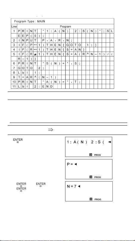
RUN
When the message “ 1: A(N), 2 :S(N) ” appears on the display, you can
input a “ P ” value to specify the type of operation to be
performed:
1 for A(N) 2 for S(N)
(1) A = 5 , R = 4, N = 7 A (N) = A (7) = 20480
[ ] ( 5 Seconds )
1 [ ] 5 [ ]
4 [ ] 7
E-78
Page 79

[ ]
(2) A = 5 , R = 4, N = 9 S (N) = S (9) = 436905
[ ] ( 5 Seconds )
2 [ ] 5 [ ]
4 [ ] 9
[ ]
(3) A = 7 ,R = 1, N = 14 S (N) = S (14) = 98
[ ] ( 5 Seconds )
2 [ ] 7 [ ]
1 [ ] 14
E-79
Page 80

[ ]
Example 58
Create a program to determine the solutions for linear equations of the
form:
RUN
[ ]
E-80
Page 81

4
[ ] [ ( – ) ] 1 [ ]
30 [ ] 5 [ ] 9
[ ] 17
[ ]
Example 59
Create three subroutines to store the following formulas and then use the
GOSUB-PROG command to write a mainroutine to execute the
subroutines.
Subroutine 1 : CHARGE = N × 3
Subroutine 2 : POWER = I A
Subroutine 3 : VOLTAGE = I ( B × Q × A )
E-81
Page 82

RUN
N = 1.5, I = 486, A = 2 CHARGE = 4.5, POWER = 243,
VOLTAGE = 2
[ ]
1.5
[ ] ( 5 Seconds )
E-82
Page 83

486
[ ] 2
[ ] ( 5 Seconds )
Example 60
Create a program that graphs Y = – and Y = 2 X with the
following range settings: X min = –3.4, X max = 3.4, X scl = 1, Y
min = –3, Y max = 3, Y scl = 1
RUN
[ ]
E-83
Page 84

[ G T ]
Example 61
Use a FOR loop to calculate 1 + 6 = ? , 1 + 5 = ? 1 + 4 = ?, 2 + 6
= ?, 2 + 5 = ? 2 + 4 = ?
RUN
[ ]
E-84
Page 85

Example 62
Set the program type to “BaseN” and evaluate
ANS = 1010 2 AND ( Y OR 7 16 )
(1) If Y = /A
[ ]
[ dhbo ] [ ] [ ] [ ]
[ ] / A
[ ]
(2) If Y =11011 8 , Ans = 1010
, Ans = 10 10
16
2
EDIT
E-85
Page 86

[ ]
[ ] [ dhbo ] [ ] [ ]
[ ]
RUN
[ ]
[ dhbo ] [ ] [ ]
[ ] 11011
[ ]
Example 63
Create a program to evaluate the following, and insert a display result
command ( ) to check the content of a memory variable
B = log ( A + 90 ), C = 13 × A, D = 51 ( A × B )
E-86
Page 87

A = 10 C = 130 , D = 2.55
[ ]
10
[ ]
[ 2nd ] [ RCL ] [ ] [ ]
[ CL/
] [ ]
ESC
RUN
E-87
Page 88

hp 9g
Calculatrice graphique
Table des Matières
Chapitre 1 : Fonctionnement général ........................... 4
Alimentation ..................................................................... 4
Allumage et extinction .................................................................. 4
Remplacement des piles ................................................................ 4
Fonction d'extinction automatique ................................................. 4
Réinitialisation .............................................................................. 4
Réglage de contraste ......................................................... 4
Caractéristiques de l'écran................................................. 5
Affichage graphique ..................................................................... 5
Affichage de calcul ....................................................................... 5
Chapitre 2 : Avant de commencer un calcul ................. 6
Changement de mode........................................................ 6
Sélection d'une option dans un menu ................................. 6
Etiquettes de touches ......................................................... 6
Utilisation des touches 2nd et ALPHA.................................. 7
Curseur............................................................................. 7
Insertion et suppression de caractères................................. 7
Rappel d'entrées et résultats précédents.............................. 7
Mémoires.......................................................................... 8
Mémoire de travail........................................................................ 8
Mémoires standard disponibles..................................................... 8
Enregistrement d'une équation ...................................................... 8
Variables de tableau ..................................................................... 8
Ordre des opérations......................................................... 9
Précision et capacité ........................................................ 10
Erreurs............................................................................ 12
Chapitre 3 : Calculs de base...................................... 13
Calculs arithmétiques....................................................... 13
F-1
Page 89

Format d'affichage.......................................................... 13
Calculs entre parenthèses................................................. 14
Calculs de pourcentage.................................................... 14
Répétitions de calculs....................................................... 14
Fonction réponse ............................................................. 14
Chapitre 4 : Calculs mathématiques courants ............. 14
Logarithme et exponentielle ............................................. 14
Calcul sur des fractions .................................................... 14
Conversion d'unités d'angle............................................. 15
Fonctions trigonométriques et trigonométriques inverses .... 15
Fonctions hyperboliques et hyperboliques inverses ............ 15
Transformations de coordonnées ...................................... 16
Fonctions mathématiques................................................. 16
Autres fonctions ( x-1, , , ,x 2, x 3, ^ ).................... 16
Conversions d'unités........................................................ 16
Constante physiques........................................................ 17
Fonctions de plusieurs expressions.................................... 18
Chapitre 5 : Graphiques ............................................ 18
Graphes de fonctions intégrées ........................................18
Graphes utilisateur .......................................................... 18
Affichage Graphique ↔ Texte et effacement d'un graphique
...................................................................................... 18
Fonction zoom................................................................. 19
Superposition de graphiques............................................ 19
Fonction de trace............................................................. 19
Défilement de graphiques ................................................ 19
Fonction de tracé et de ligne ............................................ 20
Chapitre 6 : Calculs statistiques ................................. 20
Statistiques sur une et deux variables ............................... 20
Capacité de traitement..................................................... 21
F-2
Page 90

Correction de données statistiques.................................... 21
Distribution de probabilité (données 1-Var) ....................... 22
Calculs de régression....................................................... 22
Chapitre 7 : Calculs en BaseN................................... 23
Expressions négatives...................................................... 24
Opérations arithmétiques dans d'autres bases .................. 24
Opérations logiques ........................................................ 24
Chapitre 8 : Programmation ...................................... 24
Avant d'utiliser la zone de programme ............................. 24
Instructions de contrôle de programme............................. 25
Commande d'effacement d'écran................................................ 25
Commandes d'entrée et sortie..................................................... 25
Branchement conditionnel ........................................................... 25
Commandes de branchement .......................................................26
Programmes et sous-programmes ................................................26
Incrément et décrément ................................................................26
Boucle For ....................................................................................27
Commande Sleep.........................................................................27
Commande Swap.........................................................................27
Opérateurs de comparaison............................................. 27
Création d'un programme................................................ 27
Exécution d'un programme.............................................. 28
Mise au point d'un programme........................................ 28
Utilisation de la fonction de graphique dans les programmes
...................................................................................... 28
Commande d'affichage de résultat................................... 29
Suppression d'un programme .......................................... 29
Exemples de programmes................................................ 29
F-3
Page 91

Chapitre 1 : Fonctionnement général
Alimentation
Allumage et extinction
Pour allumer la calculatrice, appuyez sur [ ON ].
Pour éteindre la calculatrice, appuyez sur [ 2nd ] [ OFF ].
Remplacement des piles
La calculatrice est alimentée par deux piles boutons alcalines (GP76A ou
LR44). Quand les piles faiblissent, le témoin LOW BATTERY apparaît à
l'écran. Remplacez les piles dès que possible.
Pour remplacer les piles :
1. Retirez le couvercle du compartiment des piles en le faisant glisser dans
le sens de la flèche.
2. Retirez les piles usées.
3. Posez des piles neuves, côté plus (+) vers l'extérieur.
4. Replacez le couvercle du compartiment des piles.
5. Appuyez sur [ ON ] pour allumer la calculatrice.
Fonction d'extinction automatique
La calculatrice s'éteint automatiquement si elle n'est pas utilisée pendant 9 à
15 minutes. Elle peut être réactivée en appuyant sur [ ON ]. L'affichage,
la mémoire et les réglages sont conservés quand la calculatrice est éteinte.
Réinitialisation
Si vous obtenez des résultats inattendus calculatrice allumée, appuyez sur
[ MODE ] ou [ CL/
[ RESET ]. Un message apparaît pour demander confirmation de la
réinitialisation de la calculatrice.
RESET : N Y
Appuyez sur [ ] pour déplacer le curseur vers Y et appuyez sur [ ].
La calculatrice est réinitialisée. Toutes les variables, programmes,
opérations en cours, données statistiques, réponses, entrées présentes en
mémoire sont effacées. Pour annuler mode de réinitialisation, déplacez le
curseur sur N et appuyez sur [ ].
Si la calculatrice se verrouille et que les touches n'ont plus aucun effet,
appuyez simultanément sur [ EXP ] [ MODE ]. Cette manœuvre
déverrouille la calculatrice et ramène tous les réglages à leurs valeurs par
défaut.
Réglage de contraste
Appuyez sur [ MODE ] puis sur [ ] ou [ ] pour augmenter ou diminuer
la luminosité de l'écran.
]. Si le problème persiste, appuyez sur [ 2nd ]
ESC
F-4
Page 92

Caractéristiques de l'écran
Affichage graphique
Graphique
Affichage de calcul
Ligne
d'entrée
Ligne d'entrée Affiche une entrée jusqu'à 76 chiffres. Les entrées
Ligne de résultat Affiche le résultat d'un calcul. 10 chiffres peuvent être
Indicateurs Les indicateurs ci-dessous apparaissent à l'écran pour
Indicateur Signification
M Des valeurs sont enregistrées dans la mémoire de travail
– Le résultat est négatif
Action incorrecte
2nd L'action suivante sera une 2
X = Y = Coordonnées x et y du pointeur de fonction de trace
STAT Le mode statistique est actif
PROG Le mode programme est actif
SCIENG Format d'affichage scientifique ou ingénieur
FIX Nombre de décimales d'affichage fixe
comportant plus de 11 chiffres défilent vers la gauche. A
l'entrée du 69
passe de à pour vous indiquer que vous
approchez la limite d'entrée. Si vous devez entrer plus de
76 chiffres, divisez votre calcul en deux ou plusieurs parties.
affichés avec un point décimal, un signe moins,
l'indicateur x10 et un exposant à 2 chiffres positif ou
négatif. Les résultats dépassant cette limite sont affichés
ème
chiffre d'une même entrée, le curseur
en notation scientifique.
indiquer l'état de la calculatrice.
ème
fonction
Les touches alphabétiques sont actives
Mode d'angle : degrés, radians ou grades
Ligne de
résultat
Ligne de
résultat
F-5
Page 93

HYP Une fonction trigonométrique hyperbolique va être calculée
La valeur affichée est un résultat intermédiaire
Il y a des chiffres à gauche ou à droite de l'affichage
Des résultats précédents ou suivants peuvent être affichés. Ces
indicateurs clignotent pendant l'exécution d'une opération ou
d'un programme.
Chapitre 2 : Avant de commencer un calcul
Changement de mode
Appuyez sur [ MODE ] pour afficher le menu de modes. Vous pouvez
choisir un des quatre modes : 0 MAIN, 1 STAT, 2 BaseN, 3 PROG.
Par exemple, pour sélectionner le mode BaseN :
Méthode 1 : Appuyez sur [ MODE ] puis sur [ ], [ ] ou
Méthode 2 : Appuyez sur [ MODE ] et entrez le numéro du mode, [ 2 ].
Sélection d'une option dans un menu
Beaucoup de fonctions et de réglages sont accessibles par des menus. Un
menu est une liste d'options affichées à l'écran.
Par exemple, l'appui sur [ MATH ] affiche un menu de fonctions
mathématiques. Pour sélectionner une de ces fonctions :
6. Appuyez sur [ MATH ] pour afficher le menu.
7. Appuyez sur [ ] [ ] [ ] [ ] pour déplacer le curseur vers la
8. Appuyez sur [ ] quand l'option est soulignée.
Pour les options de menu numérotées, vous pouvez appuyer sur [ ]
quand le nom de fonction est souligné ou entrer directement le numéro
correspondant.
Pour fermer un menu et revenir à l'affichage précédent, appuyez sur
[ CL/
Etiquettes de touches
Plusieurs des touches correspondent à plus d'une fonction. Les étiquettes
associées à une touche indique les fonctions disponibles, la couleur de
l'étiquette indiquent la méthode de sélection de la fonction.
Couleur d'étiquette Signification
Blanche Appuyez sur la touche
Jaune Appuyez sur [ 2nd ] puis sur la touche
Verte En mode Base-N, appuyez sur la touche
Bleue Appuyez sur [ ALPHA ] puis sur la touche
[ MODE ] jusqu'à souligner 2 BaseN, puis appuyez sur
[ ].
fonction à sélectionner.
].
ESC
F-6
Page 94

Utilisation des touches 2nd et ALPHA
Pour utiliser une fonction à étiquette jaune, appuyez sur [ 2nd ] puis sur la
touche correspondante. A l'appui sur la touche [ 2nd ], l'indicateur 2nd
apparaît pour indiquer que vous allez sélectionner la 2
touche suivante. Si vous appuyez sur [ 2nd ] par erreur, appuyez à
nouveau sur [ 2nd ] pour effacer l'indicateur 2nd.
L'appui sur [ ALPHA ] [ 2nd ] verrouille la calculatrice en mode 2
Ceci autorise l'entrée consécutive de fonctions secondaires. Pour annuler ce
mode, appuyez à nouveau sur [ 2nd ].
Pour accéder à une fonction à étiquette bleue, appuyez sur [ ALPHA ] puis
sur la touche correspondante. A l'appui sur [ ALPHA ], l'indicateur
apparaît pour indiquer que vous allez sélectionner la fonction alphabétique
de la touche suivante. Si vous appuyez sur [ ALPHA ] par erreur, appuyez à
nouveau sur [ ALPHA ] pour effacer l'indicateur .
L'appui sur [ 2nd ] [ ALPHA ] verrouille la calcultrice en mode alphabétique.
Ceci permet l'entrée successive de touches de fonctions alphabétiques. Pour
annuler ce mode, appuyez à nouveau sur [ ALPHA ].
ème
fonction de la
ème
fonction.
Curseur
Appuyez sur [ ] ou [ ] pour déplacer le curseur vers la gauche ou
vers la droite. Maintenez enfoncée une touche de curseur pour le déplacer
rapidement.
S'il y a des entrées ou des résultats non visibles à l'écran, appuyez sur
[ ] ou [ ] pour faire défiler l'affichage vers le haut ou vers le bas.
Vous pouvez réutiliser ou modifier une entrée précédente quand elle est sur
la ligne d'entrée.
Appuyez sur [ ALPHA ] [ ] ou [ ALPHA ] [ ] pour déplacer le curseur
au début ou à la fin de la ligne d'entrée. Appuyez sur [ ALPHA ] [ ] ou
[ ALPHA ] [
d'entrées.
Le curseur clignotant
] pour déplacer le curseur en haut ou en bas de la liste
indique que la calculatrice est en mode Insertion.
Insertion et suppression de caractères
Pour insérer un caractère, déplacez le curseur à la position voulue et entrez
le caractère. Le caractère est entré juste avant le curseur.
Pour supprimer un caractère, appuyez sur [ ] ou [ ] pour placer le
curseur sur ce caractère et appuyez sur [ DEL ]. (Quand le curseur est sur un
caractère, celui-ci est souligné). Pour annuler l'effacement, appuyez
immédiatement sur [ 2nd ] [ ].
Pour effacer tous les caractères, appuyez sur [ CL/
]. Voir Exemple 1.
ESC
Rappel d'entrées et résultats précédents
Appuyez sur [ ] ou [ ] pour afficher jusqu'à 252 caractères d'entrées,
valeurs et commandes précédentes, pour modification et réexécution. Voir
Exemple 2.
F-7
Page 95

Remarque : L'entrée précédente n'est pas effacée quand vous appuyez sur
[ CL/
] ou quand la calculatrice est éteinte, mais elle est
ESC
effacée au changement de mode.
Mémoires
Mémoire de travail
Appuyez sur [ M+ ] pour ajouter un résultat à la mémoire de travail.
Appuyez sur [ 2nd ] [ M– ] pour soustraire la valeur de la mémoire de
travail. Pour rappeler la valeur en mémoire de travail, appuyez sur [ MRC ].
Pour effacer la mémoire de travail, appuyez deux fois sur [ MRC ]. Voir
Exemple 4.
Mémoires standard disponibles
La calculatrice dispose de 26 variables de mémoire standard — A, B, C,
D, …, Z — utilisables pour l'attribution de valeurs. Voir Exemple 5. Les
opérations sur les variables sont notamment :
• [ SAVE ] + Variable attribue la réponse en cours à la variable
indiquée (A, B, C, … ou Z).
• [ 2nd ] [ RCL ] affiche un menu de variables ; sélectionnez une
variable pour rappeler sa valeur.
• [ ALPHA ] + Variable rappelle la valeur attribuée à la variable
indiquée.
• [ 2nd ] [ CL-VAR ] efface toutes les variables.
Remarque : Vous pouvez attribuer la même valeur à plus d'une variable en
Enregistrement d'une équation
Appuyez sur [ SAVE ] [ PROG ] pour enregistrer l'équation en cours en
mémoire.
Appuyez sur [ PROG ] pour rappeler l'équation. Voir Exemple 6.
Variables de tableau
En plus de 26 variables de mémoire standard (voir ci-dessus), vous pouvez
augmenter la mémoire en convertissant des pas de programme en variables
de mémoire. Vous pouvez convertir 12 pas de programme en une mémoire.
Il est possible d'ajouter au maximum 33 mémoires de cette façon, pour un
maximum de 59 mémoires (26 + 33).
une seule étape. Par exemple, pour attribuer la valeur 98 aux
variables A, B, C et D, appuyez sur 98 [ SAVE ] [ A ] [ ALPHA ]
[ ~ ] [ ALPHA ] [ D ].
Nombre de mémoires
Nombre d'octets restants
F-8
Page 96

Nombre de mémoires
Nombre d'octets restants
Remarque : Pour ramener la mémoire en configuration standard – 26
Les mémoires étendues sont appelées A [ 1 ] , A [ 2 ] etc et peuvent être
utilisées comme des variables de mémoire standard. Voir Exemple 7.
Remarque : En utilisant des variables de tableau, prenez garde à éviter le
mémoires – spécifiez Defm 0.
recouvrement des zones de mémoire. La relation est la
suivante :
Ordre des opérations
Chaque calcul est effectué en tenant compte de l'ordre de priorité suivant :
9. Fonctions à l'intérieur des parenthèses, transformations coordonnées et
fonctions de type B, c’est-à-dire pour lesquelles vous devez appuyer sur
la touche de fonction avant d'entrer l'argument, par exemple sin, cos,
tan, sin-1, cos-1, tan-1, sinh, cosh, tanh, sinh-1, cosh-1, tanh-1, log, ln, 10 X ,
e X, , , NEG, NOT, X’( ), Y ‘( ), MAX, MIN, SUM, SGN, AVG,
ABS, INT, Frac, Plot.
10. Fonctions de type A, c’est-à-dire pour lesquelles vous entrez l'argument
avant d'appuyer sur la touche de fonction, par exemple, x 2, x 3, x-1, x!,
, r, g, %,
º
11. Fonctions puissance ( ),
12. Fractions
13. Format abrégé de multiplication devant les variables, π, RAND,
RANDI.
14. ( – )
15. Format abrégé de multiplication devant les fonctions de type B, ,
Alog2, etc.
16. nPr, nCr
17. × ,
18. +, –
, ENGSYM.
º΄ ΄΄
F-9
Page 97

19. Opérateurs de comparaison : = =, < , >, ≠, ≤ , ≥
–
–
x
20. AND, NAND (calculs en BaseN seulement)
21. OR, XOR, XNOR (calculs en BaseN seulement)
22. Conversions (A b/c d/e, F D,DMS)
Quand des fonctions de même priorité sont en séquence, elles sont évaluées
de droite à gauche. Par exemple :
e X ln120 → e X { ln (120 ) }
Sinon, l'évaluation s'effectue de gauche à droite.
Les fonctions composées sont exécutées de droite à gauche.
Précision et capacité
Affihage de sortie : Jusqu'à 10 chiffres
Calcul : Jusqu'à 24 chiffres
Chaque fois que c'est possible, les calculs sont affichés jusqu'à 10 chiffres,
ou sous forme d'une mantisse à 10 chiffres avec un exposant à 2 chiffres
±99
jusqu'à 10
Les arguments entrés doivent être dans la plage acceptable pour la
fonction. Le tableau ci-dessous définit les plages d'entrée acceptées.
.
Fonctions Plages d'entrée acceptées
sin x, cos x,
tan x
Deg : x < 4.5 x 10
Rad : x < 2.5 x 10 8πrad
Grad : x < 5 x 10
10
10
grad
mais pour tan x
Deg : x ≠ 90 (2n+1)
Rad : x ≠
π
(2n+1)
2
Grad : x ≠ 100 (2n+1)
–1
sin
x, cos
–1
tan
x
sinh x, cosh x
tanh x
–1
sinh
x
–1
cosh
x
–1
tanh
x
log x, ln x
10 x
x
e
(n est un entier)
–1
x
x ≦ 1
x < 1 × 10
x ≦ 230 .2585092
x < 1 × 10
x < 5 × 10
1 ≦ x < 5 × 10
x < 1
1 × 10
1 x 10
1 × 10
0 ≦ x < 1 × 10
100
100
99
99
–99
≦ x <1 × 10
100
< x < 100
100
< x ≦ 230.2585092
100
100
deg
F-10
Page 98

x 2 x
(p
)
-1
x
x
< 1 × 10
X ! 0 ≦ x ≦ 69, x est un entier.
P ( x, y )
R (r,θ)
y+x
0 ≦ r< 1 × 10
Deg:│θ│<4.5 × 10 10 deg
< 1 × 10
22
<1 x 10
100
50
, x≠0
100
100
Rad:│θ│<2.5 × 10 8πrad
Grad:│θ│<5 × 10 10 grad
mais pour tan x
Deg:│θ│≠90 (2n+1)
Rad:│θ│≠
Grad:│θ│≠100 (2n+1)
π
(2n+1)
2
(n est un entier)
DMS
│D│, M, S < 1 × 10
0 ≦ M, S,
x
< 10
y > 0 : x≠0, -1 × 10
y = 0: x > 0
100
y < 0 : x = 2n+1, I/n, n est un entier.
nPr, nCr
STAT
(n≠0)
mais -1 × 10
0 ≦ r ≦ n, n < 10
| x | < 1×10
100
< log | y | <100
100
100
,| y | < 1×10
1 -VAR : n ≦ 30, 2 -VAR : n ≦ 30
FREQ. = n, 0 ≦ n < 10
en mode 1-VAR
σx,σ
y, x, y, a, b, r : n≠0
Sx, Sy :n≠0,1
BaseN
DEC : - 2147483648 ≦ x ≦ 2147483647
BIN :
10000000000000000000000000000000
≦x ≦
11111111111111111111111111111111
( pour négatif )
0≦x≦
01111111111111111111111111111111
(pour zéro, positif)
OCT : 20000000000≦x≦37777777777
our négatif
100
,
100
log y
<
, n, r sont entiers.
100
100
: n est un entier
<100
F-11
Page 99

0 ≦x≦17777777777 (pour zéro ou positif)
HEX : 80000000≦x≦FFFFFFFF
(pour négatif)
0≦x≦7FFFFFFF (pour zéro ou positif)
Erreurs
Lors d'une tentative de calcul interdit ou d'erreur dans un programme, un
message d'erreur apparaît brièvement quand le curseur passe sur
l'emplacement de l'erreur. Voir Exemple 3.
Les conditions suivantes donnent une erreur:
Indicateur Signification
DOMAIN Er 1. Vous avez indiqué un argument hors de la plage
DIVIDE BY O Tentative de division par 0.
OVERFLOW Er Le résultat d'un calcul dépasse les limites da la
SYNTAX Er 1. Erreur de saisie.
LENGTH Er Une entrée dépasse 84 chiffres après multiplication
OUT OF SPEC Vous avez entré une valeur CPU ou CPL négative, avec
NEST Er L'imbrication des sous-programmes dépasse 3 niveaux.
GOTO Er Il n'y a pas d'étiquette Lbl n correspondant à un GOTO
GOSUB Er 1. Il n'y a pas de PROG n correspondant à un GOSUB
2. Tentative de branchement vers une zone de programme
EQN SAVE Er Tentative d'enregistrement d'une équation dans une zone
autorisée.
2. FREQ (en statistiques 1-VAR) < 0 ou non entier.
3. USL < LSL
calculatrice.
2. Un argument incorrect a été utilisé dans une
commande ou une fonction.
3. Il manque une instruction END dans un programme.
implicite avec correction automatique.
x–USL
=C
σ3
et
PU
LSL–x
=C
PL
σ3
n.
PROG n.
qui ne contient pas de programme.
F-12
Page 100

de programme qui contient déjà un autre programme.
EMPTY Er Trentative d'exécution d'un programme depuis une zone
MEMORY Er 1. L'extension de mémoire dépasse le nombre de pas de
2. Tentative d'utilisation d'une mémoire étendue alors
DUPLICATE Le nom d'étiquette est déjà utilisé.
LABEL
Appuyez sur [ CL/
de programme qui ne contient pas d'équation ni de
programme.
programme restants.
qu'aucune mémoire n'a été étendue.
] pour effacer un message d'erreur.
ESC
Chapitre 3 : Calculs de base
Calculs arithmétiques
• Pour les opérations arithmétiques mixtes, la multiplication et la division
ont priorité sur l'addition et la soustraction. Voir Exemple 8.
• Pour les valeurs négatives, appuyez sur [ (–) ] avant d'entrer la valeur.
Voir Exemple 9.
• Les résultats supérieurs à 10
format scientifique. Voir Exemple 10.
Format d'affichage
• Pour sélectionner un format décimal, appuyez sur [ 2nd ] [ FIX ] et
sélctionnez une valeur sur le menu ( F0123456789 ). Pour définir le
nombre de décimales n, entrez directement la valeur de n, ou appuyez
sur les touches de curseur pour souligner la valeur et appuyez sur
[ ]. (La valeur par défaut est la notation en virgule flottante (F) et sa
valeur n value est •). Voir Exemple 11.
• Les formats d'affichage de nombres sont sélectionnés en appuyant sur
[ 2nd ] [ SCI/ENG ] et en choisissant un format sur le menu. Les options
du menu sont FLO (pour virgule flottante), SCI (pour scientifique) et ENG
(pour ingénierie). Appuyez sur
[ ] ou [ ] pour souligner le format voulu, puis appuyez sur [ ].
Voir Exemple 12.
• Vous pouvez entrer un nombre sous forme de mantisse et exposant par
la touche [ EXP ]. Voir Exemple 13.
• Cette calculatrice dispose aussi de 11 symboles d'entrée de valeurs en
notation ingénieur. Appuyez sur [ 2nd ] [ ENG SYM ] pour afficher les
symboles. Voir Exemple 14.
10
ou inférieurs à 10-9 sont affichés au
F-13
 Loading...