HP (Hewlett-Packard) 8753E User Manual

Download

User’s Guide

HP 8753E Network Analyzer

Rut

No. 08753-90367

Printed iu USA February 1999

Supersedes October 1998

Notice.

The information contained in this document is subject to change without notice. Hewlett-Packard makes no warranty of any kind with regard to this material, including

but not limited to, the implied warranties of merchantability and fitness for a particular

purpose.

Hewlett-Packard

shall

not be liable for errors contained herein or for incidental or

consequential damages in connection with the furnishing, performance, or use of this material.

Certification

Hewlett-Packard Company certifies that this product met its published specifications at the time of shipment from the factory. Hewlett-Packard further certifies that its calibration measurements are traceable to the United States National Institute of Standards and

‘lbchnology,

to the extent allowed by the Institute’s calibration facility, and to the calibration

facilities of other International Standards Organization members.

Wmanty

Note

The actual warranty on your instrument depends on the date it was ordered as well as whether or not any warranty options were purchased at that time. lb determine the exact warranty on your

insment,

contact the nearest Hewlett-Packard sales or service office with the model and serial number of your instrument. See the table titled “Hewlett-Packard Sales and Service Offices,” later in this section, for a list of sales and service offices.

This Hewlett-Packard instrument product is warranted against defects in material and workmanship for the warranty period. During the warranty period, Hewlett-Packard Company will, at its option, either repair or replace products which prove to be defective.

If the warranty covers repair or service to be performed at Buyer’s facility, then the service or repair will be performed at the Buyer’s facility at no charge within HP service travel areas Outside HP service travel areas, warranty service will be performed at Buyer’s facility only upon HP’s prior agreement, and Buyer shall pay HP’s round-trip travel expenses. In all other areas, products must be returned to a service facility designated by HP

If the product is to be returned to Hewlett-Packard for service or repair, it must be returned to a service facility designated by Hewlett-Packard. Buyer shall prepay shipping charges to Hewlett-Packard and Hewlett-Packard shall pay shipping charges to return the product to Buyer. However, Buyer shall pay all shipping charges, duties, and taxes for products returned

to Hewlett-Packard from another country. Hewlett-Packard warrants that its software and

lirmware

designated by Hewlett-Packard for use with an instrument will execute its programming instructions when properly installed on that instrument. Hewlett-Packard does not warrant that the operation of the instrument, or software, or

firmware

will be uninterrupted or error-free.

IMITATION OF WARRANTY

The foregoing warranty shall not apply to defects resulting from improper or inadequate maintenance by Buyer, Buyer-supplied software or interfacing, unauthorized modification or misuse, operation outside of the environmental specifications for the product, or improper site preparation or maintenance.

NO OTHER WARRANTY IS EXPRESSED OR IMPLIED. HEWLETT-PACKARD SPECIFICALLY DISCLAIMS THE IMPLIED WARRANTIES OF MERCHANTABILITY AND FITNESS FOR

PARTICULAR PURPOSE.

XCLUSIVE

MEDIES

THE REMEDIES PROVIDED HEREIN ARE BUYER’S SOLE AND EXCLUSIVE REMEDIES. HEWLETT-PACKARD SHALL NOT BE LIABLE FOR ANY DIRECT, INDIRECT, SPECIAL, INCIDENTAL, OR CONSEQUENTIAL DAMAGES, WHETHER BASED ON CONTRACT, TORT, OR ANY OTHER LEGAL THEORY.

. . .

III

Maintenance

Clean the cabinet, using a damp cloth only.

Assistance

are

Product maintenance agreements

Hewlett-&hrd Rw an@ assistance, wnmct gour nearest Hewlett-Rzchmd Saks and Service Om

products

and other customer

assktmm

agremnmts

available for

Shipment for Service

If you are sending the instrument to Hewlett-Packard for service, ship the analyzer to the nearest HP service center for repair, including a description of any failed test and any error message. Ship the analyzer, using the original or comparable anti-static packaging materials.

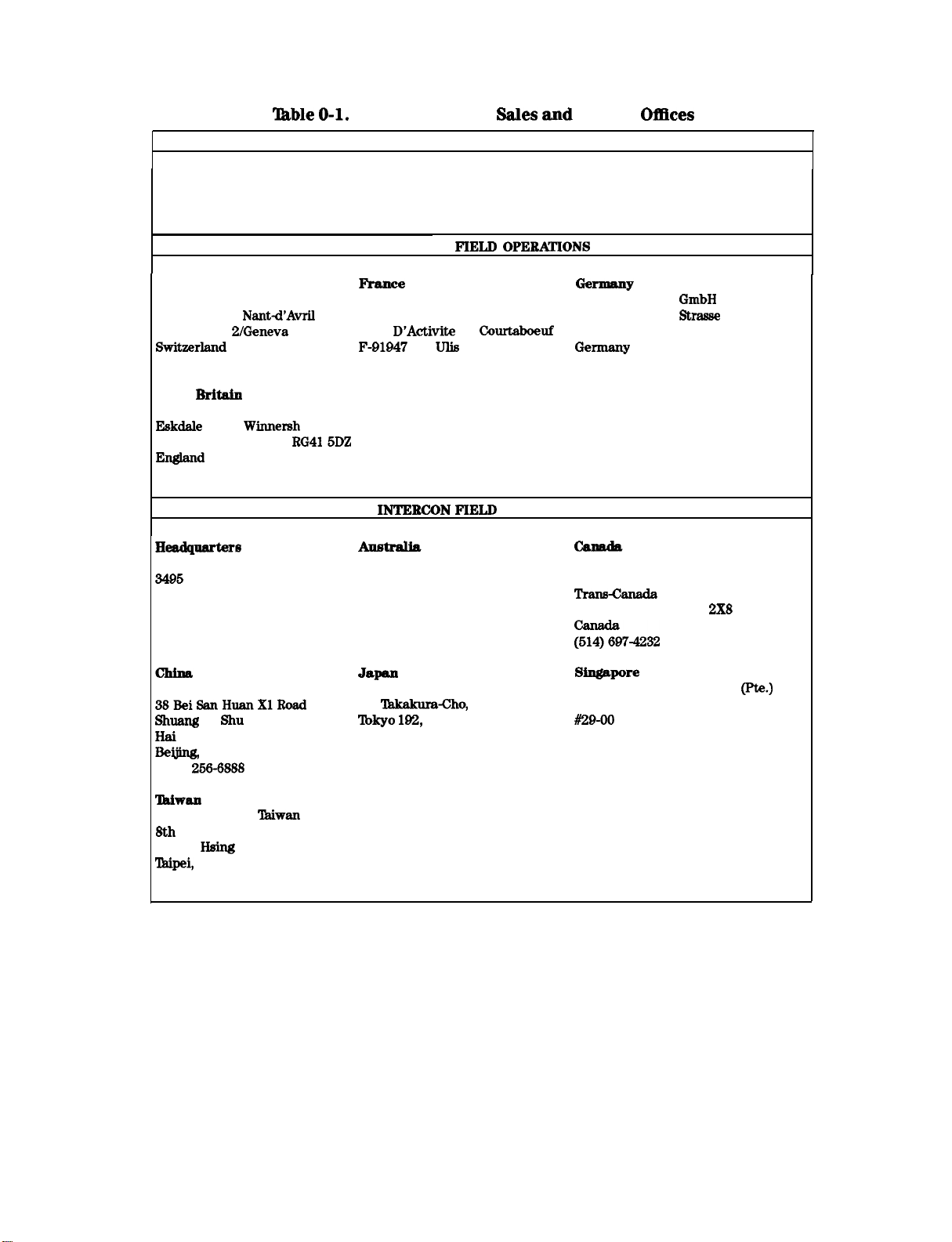
‘Iktble O-1.

Instrument Support Center Hewlett-Packard Company (800) 403-0801

Hewlett-Packard

UNITED STATES

Sales

and Service

OfEces

EUROPEAN

Headquarters Hewlett-Packard S.A. 150, Route du 1217 Meyrin

&vi&&and

(41 22) 780.8111 France Great

Hewlett-Packard Ltd.

E&dale Road,

Woldngham, Berkshire

England

(44 734) 696622

HWkpWtt%S

Hewlett-Packard Company

3495

Deer Creek Road Palo Alto, California, USA 94304-1316 (415) 857-5027

Nantd’Avril

Z/Geneva

Britah

Whmersh

RG415DZ

Triangle

Prame

Hewlett-Packard France Hewlett-Packard

1 Avenue Du Canada Zone D’Activite De

F-91947

(33 1) 69 82 60 60

Hewlett-Packard Australia Ltd. 31-41 Joseph Street Blackbum, Victoria 3130 (61 3) 895-2895

Les

INTERCON

JspaJp

China Hewlett-Packard Company Hewlett-Packard Japan, Ltd.

38BeiSanHuanXlRoad aulaug

shu Hai Dian District Beijin&

china

(86 1)

256-6888

Q-l %kakuraCho, Hachioji

lblcyo 192,

(81 426) 60-2111

FIELD OPEEA!l’IONS

Courtaboeuf

Ulis

Cedex

FIELD

OPERATIONS

Japan

G-m=w

Hewlett-Packard 61352 Bad Homburg v.d.H

Germany

(49 6172)

Hewlett-Packard (Canada) Ltd. 17500 South Service Road

TramCanada

Kirkland, Quebec HQJ

z7-4232

fb@me

Hewlett-Packard Singapore (Pte.) Ltd. 150 Beach Road

#29-00

Singapore 0718 (65) 291-9088

GmbH Strasse

16-O

Highway

2X8

Gateway West

IkbiWSn

Hewlett-Packard

8th Floor, H-P Building

337 Fu

I-king

Tkdpei,

Taiwan

(886 2) 712-0404

‘&wan

North Road

Safety Symbols

The following safety symbols are used throughout this manual. of the symbols and its meaning before operating this instrument.

Caution

Warning

Caution denotes a hazard. It calls attention to a procedure that, if not correctly performed or adhered to, would result in damage to or destruction of the instrument. Do not proceed beyond a caution note until the indicated conditions are fully understood and met.

Rkning

correctly performed or adhered to, could result in injury or loss of life. Do not proceed beyond a warning note until the indicated conditions are fully understood and met.

denotes a hazard. It calls attention to a procedure which, if not

Familiarize

yourself with each

Instrument Markings

is necessary for the user to refer to the instructions in the documentation. “CE” The CE mark is a registered trademark of the European Community. (If accompanied by

a year, it is when the design was proven.)

The instruction documentation symbol. The product is marked with this symbol when it

“ISMl-A”

“CSA” The CSA mark is a registered trademark of the Canadian Standards Association.

This is a symbol of an Industrial Scientific and Medical Group 1 Class A product.

General Safety Considerations

Note

Warning

Caution

Warning

This instrument has been designed and tested in accordance with IEC

Publication 1010, Safety Requirements for Electronics Measuring Apparatus,

and has been supplied in a safe condition. This instruction documentation

contains information and warnings which must be followed by the user to

ensure safe operation and to maintain the instrument in a safe condition.

This is a ground incorporated in the power cord). The mains plug shall only be

inserted in a socket outlet provided with a protective earth contact. Any

interruption of the protective conductor, inside or outside the instrument,

is likely to make the instrument dangerous. Intentional interruption is prohibited.

No operator serviceable parts inside. Refer servicing to qualified

personnel. lb prevent electrical shock, do not remove covers.

Before switching on this instrument, make sure that the line voltage selector switch is set to the voltage of the power supply and the correct fuse is installed. Assure the supply voltage is in the specified range.

The opening of voltages.

being opened.

safety

Class I product (provided with a protective earthing

covers

DiSCOMeCt

or removal of parts is likely to expose dangerous

the instrument from all voltage sources while it is

Warning

The power cord is connected to

for 10 seconds after disconnecting the plug from its power supply.

For continued protection against

same type and rating (F prohibited.

lb prevent electrical shock, disconnect the HP 87533 from mains before

cleaning. Use a dry cloth or one slightly dampened with water to clean

the external case parts. Do not attempt to clean internally.

If this product is not used as

equipment could be impaired. This product must be used in a normal condition (in which all means for protection are intact) only.

Always use the three-prong AC power cord supplied with this product.

FMlure

cause product damage.

to ensure adequate earth grounding by not using this cord may

3A/250V).

internal capacitors that may remain live

fire

hazard replace line fuse only with

The use of other fuses or material is

specitled,

the protection provided by the

Caution

This product is designed for use in Installation Category II and Pollution Degree 2 per IEC 1010 and 664 respectively.

Caution

Warning

VENTILATION REQUIREMENTS: When convection into and out of the product must not be restricted. The ambient temperature (outside the cabinet) must be less than the maximum operating temperature of the product by 4O C for every 100 watts dissipated in the cabinet. If the total power dissipated in the cabinet is greater that 800 watts, then forced convection must be used.

Install the instrument according to the enclosure protection provided. This instrument does not protect against the ingress of water. This

iustrument protects agaius

enclosure.

finger

instaIling

access to hazardous parts within the

the product in a cabinet, the

Compliance with German FTZ Emissions Requirements

This network analyzer complies with German Emission requirements.

FlZ

526/527 Radiated Emissions and Conducted

Compliance with German Noise Requirements

This is to declare that this instrument is in conformance with the German Regulation on Noise Declaration for Machines (Laermangabe nach der Maschinenlaermrerordung -3. GSGV Deutschland).

Acoustic Noise

LpA<70 dB

Emission/Geraeuschemission

Lpa<70 dD

User’s Guide Overview

Chapter 1, “HP 8753E Description and Options, ndescribes features, functions, and available

options.

Chapter 2, “Making Measurements,” contains step-by-step procedures for making

measurements or using particular functions.

Chapter 3, “Making Mixer Measurements,

contains step-by-step procedures for making

calibrated and error-corrected mixer measurements.

Chapter 4, “Printing, Plotting, and Saving Measurement Results,” contains instructions

for saving to disk or the analyzer internal memory, and printing and plotting displayed measurements.

Chapter 5, “Optimizing Measurement Results,

describes techniques and functions for

achieving the best measurement results

Chapter 6, “Application and Operation Concepts,

contains explanatory-style information

about many applications and analyzer operation.

Chapter 7, “Specifications and Measurement Uncertainties,” defines the performance

capabilities of the analyzer.

Chapter 8, “Menu Maps,” shows softkey menu relationships.

Chapter 9, “Key Dell&ions,” describes all the front panel keys, softkeys, and their

corresponding HP-IB commands.

Chapter 10, “Error Messages,” provides information for interpreting error messages

Chapter 11, “Compatible Peripherals,

lists measurement and system accessories, and other applicable equipment compatible with the analyzer. Procedures for configuring the peripherals, and an HP-IB programming overview are

Chapter 12, “Preset State and Memory Allocation,”

also

included.

contains a discussion of memory

allocation, memory storage, instrument state definitions, and preset conditions.

Appendix A, “The the

CITIGle

Appendix B, “Determining System Measurement Uncertainties,” contains information on how

data format as well as a list of

CITIlile

Data Format and Key Word Reference,

CITIflle

keywords

contains information on

to determine system measurement uncertainties.

Network Analyzer Documentation Set

The Installation and Quick Start Guide

familiarizes you with the network analyzer’s front and rear panels, electrical and environmental operating requirements, as well as procedures for installing, configuring, and verifying the operation of the analyzer.

The User’s Guide

shows how to make measurements, explains commonly-used features, and tells you how to get the most

performance from your analyzer.

The Quick Reference Guide

provides a

summary of selected user features.

The

HEW3

Programming and Command

Reference Guide

provides programming information for operation of the network analyzer under HP-IB control.

The HP BASIC Programming Examples Guide

provides a tutorial introduction using BASIC programming examples to demonstrate the remote operation of the network analyzer.

The System

Vertication

and

‘lkst

Guide

provides the system verification and performance tests and the Performance Test Record for your analyzer.

DECLARATION OF CONFORMITY

Manufacturer’s Name:

According to ISO/IEC Guide 22 and EN 45014

Hewlett-Packard Co.

Hewlett-Packard Japan, Ltd.

Manufacturer’s Address:

Microwave Instruments Division 1400 Fountaingrove Parkway

Santa Rosa, CA

95403-I

799

USA

Kobe Instrument Division

l-3-2,

Murotani, Nishi-ku, Kobe-shi

Hyogo, 651-22

Japan

Declares that the product:

Product Name: Model Number: Product Options:

Network Analyzer

8753E

This declaration covers all options of the above product

Conforms to the following Product specifications:

Safety: IEC

61010-1:199O/EN 61010-I:1993

CAN/CSA-C22.2 No. 1010.1-92

EMC:

CISPR 11:1990/EN

IEC

801-2:199l/EN

IEC

801-3:1984/EN

IEC

801-4:1988/EN 50982-I :I

5501

I:1991

Group I, Class A 50082-I:1992 4 kV CD, 8 kV AD 50082-I:1992 3 V/m, 27-500 MHz

992 0.5 kV sig. lines, 1 kV power lines

Supplenientary Information:

The product herewith complies with the requirements of the Low Voltage Directive

73/23/EEC

Jo HiaWQuality

Europeen Contact: Your knxl Hewlett-Packard Sales and Servke Oftice or Hewlett-Packard GmbH Department HQ-

TFIE, Heneneberger Strasse 130. D71034 Boblingen, Germany (FAX +49-7031-U-3143

and the EMC Directive

Engineering Manager

Santa Rosa, 21 Jan. 1998

89/336/EEC

and carries the CE-marking accordingly.

Obara/Quality Engineering Manager

Mike

Kobe, 14 Jan. 1998

xii

Contents

HP 8753E Description and Options

Where to Look for More Information Analyzer Description Front Panel Features Analyzer Display Rear Panel Features and Connectors Analyzer Options Available

Option lD5, High Stability Frequency Reference Option 002, Harmonic Mode Option Option 010, Time Domain Option 011, Receiver Configuration Option 075,750 Impedance Option Option

Option Service and Support Options Differences among the HP 8753 Network Analyzers

B¶akiug

Where to Look for More Information Principles of Microwave Connector Care Basic Measurement Sequence and Example

Basic Measurement Sequence

Basic Measurement Example

Using the Display Functions

‘Ib

lb View the Measurement Data and Memory Trace

lb Subtract the Memory Trace from the Measurement Data Trace

‘IbRatioMeasurementsinChannelland2

‘Ib Title

Using the Four-Parameter Display

Four-Parameter Display and Calibration

‘lb

Quick Four-Parameter Display

006,6 GHz

lDT,

Delete Display

lCM,

Rack Mount Flange Kit Without Handles

lCP,

Rack Mount Flange Kit With Handles

Measurements

Step 1. Connect the device under test and any required test equipment. Step 2. Choose the measurement parameters.

Setting the Frequency Range Setting the Source Power.

Setting the Measurement Step 3. Perform and apply the appropriate error-correction. Step 4. Measure the device under test. Step 5. Output the measurement results.

View Both Primary Measurement Channels Save a Data Trace to the Display Memory

Divide Measurement Data by the Memory Trace

the Active Channel Display

View AR Four S-Parameters of a Two-Port Device lb Activate and Configure the Auxiliary Channels

.............................

..............................

..........................

Operation

.........................

........................

.........................

.....................

........................

.....................

......................

.......................

.....................

.......................

...............

............

..............

...................

..................

...............

........

..................

.................

................

.............

.......

.................

...................

.............

l-l

l-2 l-4

l-7 l-11

1-13 1-13 1-13 1-13 1-13 1-13 1-13 1-13 1-13 1-14 1-14 1-15

2-l

2-2 2-3 2-3 2-3 2-3 2-3 2-3 2-4 2-4

2-4

2-5 2-5

2-6 2-6

2-7 2-7 2-8 2-8 2-8 2-9

2-10 2-10 2-10 2-12

2-13

conttmts-1

Characterizing a Duplexer . . . . . . . . . . . . . . . . . . . . . . . . . .

Required Equipment . . . . . . . . . . . . . . . . . . . . . . . . . . . .

Procedure for Characterizing a Duplexer . . . . . . . . . . . . . . . . . .

Using Analyzer Display Markers . . . . . . . . . . . . . . . . . . . . . . .

‘Ib

Use Continuous and Discrete Markers . . . . . . . . . . . . . . . . . .

Activate Display Markers . . . . . . . . . . . . . . . . . . . . . . . .

Move Marker Information off of the Grids . . . . . . . . . . . . . . . .

‘Ib

Use Delta (A) Markers . . . . . . . . . . . . . . . . . . . . . . . . . .

To Activate a.Fixed.@.arker

Using the ~~~~~~~~~.~

Using

the

~~~~~~~

Couple and Uncouple Display Markers . . . . . . . . . . . . . . . . . .

..:...i .:: .i

. . . . . . . . . . . . . . . . . . . . . . . . . . . . . .

Key

I..

.,.::

;.:::

. . . . .

;;..:.:.:

. . . . . .

Key

to Activate a Fixed Reference Marker

to A&iv&e a F&d Reference Marker

. .

. . . . . .

lb Use Polar Format Markers . . . . . . . . . . . . . . . . . . . . . . . .

TbUseSmithChartMarkers

. . . . . . . . . . . . . . . . . . . . . . . .

lb Set Measurement Parameters Using Markers . . . . . . . . . . . . . . .

Setting the Start Frequency . . . . . . . . . . . . . . . . . . . . . . .

Setting the Stop Frequency . . . . . . . . . . . . . . . . . . . . . . . .

Setting the Center Frequency . . . . . . . . . . . . . . . . . . . . . . .

Setting the Frequency Span . . . . . . . . . . . . . . . . . . . . . . .

Setting the Display Reference Value . . . . . . . . . . . . . . . . . . . .

Setting the Electrical Delay. . . . . . . . . . . . . . . . . . . . . . . .

Setting the CW Frequency . . . . . . . . . . . . . . . . . . . . . . . . .

‘RI

Search for a Specific Amplitude . . . . . . . . . . . . . . . . . . . . .

Searching for the Maximum Amplitude . . . . . . . . . . . . . . . . . .

Searching for the Minimum Amplitude . . . . . . . . . . . . . . . . . .

Searching for a

‘lhrget

Amplitude . . . . . . . . . . . . . . . . . . . . .

Searching for a Bandwidth . . . . . . . . . . . . . . . . . . . . . . . .

Tracking the Amplitude that You Are Searching . . . . . . . . . . . . . .

‘RI

Calculate the Statistics of the Measurement Data . . . . . . . . . . . . .

Measuring Magnitude and Insertion Phase Response . . . . . . . . . . . . . .

Measuring the Magnitude Response . . . . . . . . . . . . . . . . . . . . .

Measuring Insertion Phase Response . . . . . . . . . . . . . . . . . . . .

Measuring Electrical Length and Phase Distortion . . . . . . . . . . . . . . .

Measuring Electrical Length . . . . . . . . . . . . . . . . . . . . . . . .

Measuring Phase Distortion . . . . . . . . . . . . . . . . . . . . . . . . .

Deviation From Linear Phase . . . . . . . . . . . . . . . . . . . . . . .

Group Delay . . . . . . . . . . . . . . . . . . . . . . . . . . . . . . .

TestingADevicewithLimitLines

. . . . . . . . . . . . . . . . . . . . . .

Setting Up the Measurement Parameters . . . . . . . . . . . . . . . . . .

Creating Flat Limit Lines . . . . . . . . . . . . . . . . . . . . . . . . . .

CreatingaSlopingLimitLine

. . . . . . . . . . . . . . . . . . . . . . . .

Creating Single Point Limits . . . . . . . . . . . . . . . . . . . . . . . .

Editing Limit Segments. . . . . . . . . . . . . . . . . . . . . . . . . . .

Deleting Limit Segments . . . . . . . . . . . . . . . . . . . . . . . . .

RtmningaLimitTest

. . . . . . . . . . . . . . . . . . . . . . . . . . . .

Reviewing the Limit Line Segments . . . . . . . . . . . . . . . . . . . .

ActivatingtheLimitlbst

. . . . . . . . . . . . . . . . . . . . . . . . .

Offsetting Limit Lines . . . . . . . . . . . . . . . . . . . . . . . . . . .

Measuring Gain Compression . . . . . . . . . . . . . . . . . . . . . . . . .

Measuring Gain and Reverse Isolation Simultaneously . . . . . . . . . . . . .

Measurements Using the Swept List Mode . . . . . . . . . . . . . . . . . . .

Connect the Device Under

Test

. . . . . . . . . . . . . . . . . . . . . . .

Observe the Characteristics of the Filter . . . . . . . . . . . . . . . . . .

Choose the Measurement Parameters . . . . . . . . . . . . . . . . . . . .

2-13 2-14 2-14 2-17 2-17 2-18

2-19

2-20 2-21 2-22

2-23 2-24

2-24 2-25 2-26 2-27 2-27 2-28 2-29 2-30 2-31 2-31 2-32

2-32

2-33 2-34 2-35 2-35

2-36

2-37 2-37 2-38 2-40

2-40

2-42 2-42

2-43 2-46 2-46

2-47

2-49

2-51

2-52

2-53

2-54

2-55

2-59

2-61

2-61 2-62

2-62

Set Up the Lower Set Up the

Passband

Set Up the Upper

Calibrate and Measure

Measurements Using the Tuned Receiver Mode

Typical test setup Tuned receiver mode in-depth description

Frequency Range

Compatible Sweep Types

External Source Requirements Test Sequencing Creating a Sequence

Running a Sequence

Stopping a Sequence Editing a Sequence

Deleting Commands Inserting a Command Modifying a Command

Clearing a Sequence from Memory Changing the Sequence

Naming

Files

Generated by a Sequence Storing a Sequence on a Disk Loading a Sequence from Disk Purging a Sequence from Disk Printing a Sequence Cascading Multiple Example Sequences Loop Counter Example Sequence Generating Limit

Files

Test

Example Sequence Measuring Swept Harmonics (Option 002 Measuring a Device in the Time Domain (Option 010

Transmission Response in Time Domain Reflection Response in Time Domain

Non-coaxial Measurements

Stopband

Parameters

Stopband

Parameters

.....................

Parameters

..................

...........................

................

.............................

..................

............................

.........................

......................

...............................

.............................

............................

...........................

..........................

.....................

Title

........................

....................

........................

.......................

............................

...................

......................

in a Loop Counter Example Sequence

............

........................

only)

................

only)

...................

....................

..........................

...........

2-63 2-63

2-63 2-64 2-66 2-66 2-66 2-66 2-66

2-67

2-68

2-69 2-70 2-70 2-71

2-71 2-71 2-72

2-72 2-73 2-73

2-74 2-75 2-75

2-75 2-76 2-77 2-78 2-79 2-81 2-83 2-83 2-88 2-91

Making Mixer Measurements

Where to Look for More Information Measurement Considerations

.........................

Source and Load Mismatches Reducing the Effect of Spurious Responses

EliminatingUnwantedMirringandLeakageSignals. HowRFandIFAreDefIned

Frequency Offset Mode Operation

.....................

..................

.................

.............

........................

......................

Differences Between Internal and External R Channel Inputs Power Meter Calibration

Conversion Loss Using the Frequency Offset Mode High Dynamic Range Swept RF/IF Conversion Loss Fixed IF Mixer Measurements

Tuned Receiver Mode Sequence 1 Setup Sequence 2 Setup

.............................

Phase or Group Delay Measurements Amplitude and Phase Tracking Conversion Compression Using the Frequency Offset Mode Isolation Example Measurements

..........................

...............

..............

........................

...........................

.....................

........................

...........

.......................

.........

3-l

3-2

3-2 3-4

3-4

3-6 3-7

3-12 3-17 3-17 3-17 3-21 3-24

3-27

3-28 3-33

LO to RF Isolation RF Feedthrough

Printing, Plotting, and Saving Measurement Results

Where to Look for More Information

Printing or Plotting Your Measurement Results Configuring a Print Function

DeIIning

a Print Function

IfYouAreUsingaColorPrinter ‘Ib

Reset the Printing Parameters to Default Values Printing One Measurement Per Page Printing Multiple Measurements Per Page

Conllguring

a Plot Function If You Are Plotting to an If You Are Plotting to a Pen Plotter

If You Are Plotting to a Disk Drive

Defining

a Plot Function Choosing Display Elements Selecting Auto-Feed Selecting Pen Numbers and Colors Selecting Line Types

Choosing

Scale.

Choosing Plot Speed lb Reset the Plotting Parameters to Default Values

Plotting One Measurement Per Page Using a Pen Plotter Plotting Multiple Measurements Per Page Using a Pen Plotter

If You Are Plotting to an HPGL Compatible Printer

Plotting a Measurement to Disk

TbOutputthePlotFiles

TbViewPlotFilesonaPC

usingAmiPr0

Using Freelance Outputting Plot Files from a PC to a Plotter Outputting Plot Files from a PC to an HPGL Compatible Printer

Step 1. Store the HPGL initialization sequence.

Step 2. Store the exit HPGL mode and form feed sequence.

Step 3. Send the HPGL

Step 4. Send the plot

.............................

..............................

.....................

................. 4-3

......................... 4-3

..........................

...................... 4-6

..............

.....................

...................

.........................

HPGLIB

Compatible Printer

............. 4-8

.....................

...........................

.........................

............................

.....................

............................

..............................

............................

..............

............

..........

.............

........................

..........................

...............................

..............................

..................

........

...............

.........

initiahzation

flIe

to the printer.

sequence to the printer.

...................

.........

Step 5. Send the exit HPGL mode and form feed sequence to the printer.

OutputtingSiiePagePlotsUsingaPrinter.

Outputting Multiple Plots to a Siie Page Using a Printer Plotting Multiple Measurements Per Page From Disk

ToPlotMultipleMeasurementsonaFullPage ‘Ib

Plot Measurements in Page Quadrants

Titling the Displayed Measurement

......................

Con6guringtheAnalyzertoProduceaTimeStamp AbortingaPrintorPlotProcess

Printing or Plotting the List

IfYouWantaSiiePageofValues

Values

.......................

or Operating Parameters

.....................

IfYouWanttheEntireListofVaIues

Solving Problems with Printing or Plotting Saving and

Places Where You Can Save

Recalling

Instrument States

........................

What You Can Save to the Analyzer’s Internal Memory

WhatYouCanSavetoaFloppyDisk

.................

...........

..............

................

..................

..............

..........

....................

..................

....................

............

....................

...

3-33

3-35

4-2

4-5

4-6

4-7 4-8

4-10

4-11 4-12 4-12 4-12

4-13 4-14 4-15 4-15 4-16 4-16 4-17 4-18 4-19

4-20 4-20

4-21 4-22 4-22 4-23 4-23 4-24 4-24 4-24 4-24 4-24 425 4-26 4-26 4-28 4-29 4-30

4-30 4-30 4-30

4-31

4-32

4-33

4-33 4-33

4-33

Contentsll

What You Can Save to a Computer Saving an Instrument State Saving Measurement Results

ASCII Data Formats

CITIille

S2P

.................................

Data Format. Re-Saving an Instrument State Deleting a File

................................

..........................

.........................

............................

........................

lb Delete an Instrument State File

IbDeleteaIlFiles RenamingaFile RecallingaFile

Formatting a Disk

.............................

...............................

..............................

Solving Problems with Saving or Recalling

IfYouAreUsinganExtemalDiskDrive.

.....................

Files

................

..................

4-34 4-35 4-36

4-39

4-39 4-39 4-41 4-41

4-41 4-41

4-42 4-42 4-43

4-43

5. Optimizing Measurement

Where to Look for More Information Increasing Measurement Accuracy

Connector Repeatability

Interconnecting Cables Temperature Drift Frequency Drift

..............................

Performance Verification Reference Plane and Port Extensions

Measurement Error-Correction

Conditions Where Error-Correction is Suggested Types of Error-Correction Error-Correction Stimulus State Calibration Standards

Compensating for the Electrical Delay of Calibration Standards Clarifying Type-N Connector Sex

When to Use Interpolated Error-Correction

Procedures for Error-Correcting Your Measurements Frequency Response Error-Corrections

Response Error-Correction for Reflection Measurements Response Error-Correction for Transmission Measurements Receiver Calibration

Frequency Response and Isolation Error-Corrections

Response and Isolation Error-Correction for Reflection Measurements

Results

.....................

......................

..........................

...........................

.............................

..........................

....................

........................

...............

.........................

.......................

...........................

.......

.....................

.................

..............

....................

...........

..........

............................

..............

.....

Response and Isolation Error-Correction for Transmission Measurements

One-Port Reflection Error-Correction Full Two-Port Error-Correction

TRL*

and

TRM*

Error-Correction TRL Error-Correction TRM Error-Correction

...........................

Modifying Calibration Kit Standards

Definitions

................................

Outline of Standard Modification Modifying Standards Modifying TRL Standards. Modifying TRM Standards

............................

.........................

Power Meter Measurement Calibration

Entering the Power Sensor Calibration Data

Editing Frequency Segments

.....................

........................

.......................

......................

....................

.................

.......................

...

5-2 5-2 5-2 5-2 5-2 5-3 5-3 5-3 5-4 5-4

5-5 5-6

5-6

5-6 5-6 5-8 5-9

5-9 5-11 5-12

5-14 5-14 5-16 5-18 5-21

5-24

5-25 5-27 5-27

5-27

5-27 5-29 5-31

5-34

5-35

Contents-6

Deleting Frequency Segments Compensating for Directional Coupler Response Using Sample-and-Sweep Correction Mode Using Continuous Correction Mode

lb Calibrate the Analyzer Receiver to Measure Absolute Power

Calibrating for Noninsertable Devices

Adapter Removal

.............................

Perform the 2-port Error Corrections Remove the Adapter Verify the Results Example Program

Matched Adapters

...........................

............................

.............................

ModifytheCalKitThruDellnition

Making Accurate Measurements of Electrically Long Devices

The Cause of Measurement Problems lb Improve Measurement Results

Decreasing the Sweep Rate Decreasing the Time Delay

Increasing Sweep Speed

‘IbUseSweptListMode

Detecting IF Delay

Decrease the Frequency Span

...........................

..........................

............................

TbSettheAutoSweepTimeMode To

Widen the System Bandwidth lb Reduce the Averaging Factor

Reduce the Number of Measurement Points

‘IbSettheSweepType. To

View a Siie Measurement Channel

Activate Chop Sweep Mode

..........................

lb Use External Calibration

Use Fast

Increasing Dynamic Range

TIbIncreasetheTestPortInputPower

2-Port

Calibration

..........................

lb Reduce the Receiver Noise Floor

Changing System Bandwidth

Changing Measurement Averaging

Reducing Trace Noise

‘lb Activate Averaging

............................

...........................

‘Ib Change System Bandwidth

Reducing Receiver Crosstalk Reducing

RecaIl

Time

............................

Understanding Spur Avoidance

......................

...............

..................

.....................

.......

.....................

...................

.....................

..........

....................

......................

........................

......................

.....................

......................

................

...................

.......................

........................

.......................

....................

.....................

.......................

....................

.......................

.........................

.......................

5-36 5-36 5-37 5-38

5-39

5-40 5-41

5-42 5-43 5-44 5-45 5-46 5-47 5-48 5-48 5-48 5-48 5-49 5-50

5-50

5-50 5-51 5-51 5-52

5-52

5-52 5-53 5-53

5-54

5-56 5-56 5-56

5-56

5-57 5-57 5-57

5-57 5-58 5-59

Application and Operation Concepts

Where to Look for More Information HP 8753E System Operation

The

Built-In

Synthesized Source

The Source Step Attenuator

The Built-In

Test

The Receiver Block The Microprocessor

............................

Set

............................

Required Peripheral Equipment

Data Processing

Processing Details

TheADC

Contents-6

...............................

.............................

................................

.....................

.........................

......................

.......................

6-l

6-2 6-2 6-2 6-3 6-3

6-3 6-3 6-4 6-5 6-5

IF Detection Ratio Calculations Sampler/IF Correction Sweep-lb-Sweep Averaging Pre-Raw Data Arrays Raw Arrays Vector Error-correction (Accuracy Enhancement)

Trace

Math Operation Gating (Option 010 The Electrical Delay Block Conversion Transform (Option 010 Format Smoothing Format Arrays

OffsetandScaIe

Display Memory

Active Channel Keys

AuxiIiary

Channels and Two-Port Calibration

Enabling AuxiIiary

Multiple Channel Displays Uncoupling StimuIus Coupled Markers

Entry Block Keys

Units Terminator. Knob

...................................

StepKeys

...............................

............................

..........................

........................

..........................

...............................

.............

..........................

only)

.........................

........................

...............................

only)

.......................

.................................

................................

..............................

.............................

................

Channels

........................

.........................

Values

Between Primary Channels

...........

..............................

.............................

.................................

gqiif)

......................................................................

Modifying or Deleting Entries

TurningofftheSoftkeyMenu

.....................................

....................................

StimuIus Functions

Defining Ranges with

StimuIus Menu.

The Power Menu.

.............................

Stimulus

..............................

Understanding the Power Ranges

Automatic mode Manual mode

Power

Coupling

Channel

Test

port

SweepTime

coupling

couphng

.................................

.............................

..............................

Options

............................

Manual Sweep Time Mode Auto Sweep Time Mode Minimum Sweep Time

TriggerMenu..

...........................

..............................

Source Attenuator Switch Protection

Allowing Repetitive Switching of the Attenuator

Channel Sweep Type Menu

Linear

stimulus Coupling

..............................

Frequency Sweep (Hz) Logarithmic Frequency Sweep (Hz) Stepped List Frequency Sweep (Hz)

.......................

......................

Keys

....................

......................

..........................

.........................

..........................

.....................

..............

..........................

........................

.....................

6-5

6-6 6-6

6-6 6-6 6-6 6-6

6-6 6-7

6-7 6-7

6-7

6-8 6-8 6-9 6-9

6-9

6-10 6-10 6-10 6-11 6-11 6-11

6-11

6-11 6-11 6-12 6-12 6-13 6-14

6-14 6-14 6-14 6-16 6-16

6-16

6-17 6-17

6-19 6-20 6-20 6-21

6-22

6-23

Contentsd

Segment Menu. Stepped Edit List Menu Stepped Edit

Swept List Frequency Sweep (Hz)

Swept Edit List Menu Swept Edit Setting Segment Power

Setting Segment IF Bandwidth Power Sweep CW Time Sweep (Seconds) Selecting Sweep Modes

Response Functions S-Parameters

Understanding S-Parameters The S-Parameter Menu

Analog In Menu

Conversion Menu

Input Ports Menu

The Format Menu

Log Magnitude Format Phase Format Group Delay Format Smith Chart Format Polar Format Linear Magnitude Format.

SWRFormat RealFormat

Imaginary Format

Group Delay Principles

Scale

Reference Menu

Electrical Delay

Display Menu

Dual

Channel Mode

Dual

Channel Mode with Decoupled Stimulus

.............................

.........................

Subsweep

......................

...................... 6-25

..........................

Subsweep

....................... 6-25

..........................

......................

(dBm)

............................ 6-27

.........................

...........................

.............................

................................

........................ 6-29

...........................

.............................

............................

..............................

...........................

...............................

............................

...............................

.........................

................................

.............................

...........................

............................

..............................

................................

............................

...............

Dual Channel Mode with Decoupled Channel Power

Four-Parameter Display Functions

Customizing the Display Channel Position Softkey

Param

Displays

Softkey

Memory Math Functions

.........................

..........................

Adjusting the Colors of the Display

Setting Display Intensity Setting Default Colors Blanking the Display Saving

Modiiied

Colors Recalling Modified Colors The Modify Colors Menu

Averaging Menu

Averaging Smoothing

...............................

.................................

IF Bandwidth Reduction

Markers

Marker Menu

...................................

...............................

Delta Mode Menu

Fixed Marker Menu

.........................

..........................

...........................

..........................

.........................

..........................

............................

..........................

.....................

............

6-23 6-23

6-24 6-25 6-25

6-26 6-27

6-27 6-28 6-29

6-30 6-30 6-30

6-31

6-32 6-32 6-33 6-33

6-34

6-35 6-36 6-36 6-37 6-37 6-38

6-41 6-41

6-42 6-43 6-43

6-43

6-45 6-45 6-46

6-46

6-48

6-48 6-48 6-49 6-49 6-49 6-49 6-49

6-51

6-52 6-52

6%&

6-55

Contents-ll

Marker

Function

Marker Search Menu

lhrget Menu

..............................

Marker Mode Menu

Polar Marker Menu Smith Marker Menu

Measurement Calibration

What Is Accuracy Enhancement?

What Causes Measurement Errors?

Directivity Source Match Load Match

...............................

..............................

...............................

Isolation (Crosstalk) Frequency Response (Tracking)

Characterizing Microwave Systematic Errors

One-Port Error Model Device Measurement ‘Iwo-Port Error Model

Calibration Considerations

Measurement Parameters

Device Measurements Omitting Isolation Calibration Saving Calibration Data The Calibration Standards Frequency Response of Calibration Standards

Electrical Offset

Pringe

Capacitance

How Effective Is Accuracy Enhancement?

Correcting for Measurement Errors

Ensuring a Valid Calibration Interpolated Error-correction

The Calibrate Menu

Response Calibration Response and Isolation Calibration

Sll

and s2 One-Port Calibration Pull Two-Port Calibration.

TRL*/LRM*

Two-Port Calibration Restarting a Calibration

CalKitMenu

................................

TheSelectCalKitMenu

Modifying Calibration Kits

Definitions Procedure

................................

.................................

Modify Calibration Kit Menu

Defme

Standard Menus.

Specify Offset Menu

Label Standard Menu

Specify Class Menu Label Class Menu Label Kit Menu

Verify performance

TRL*/LRM*

Calibration Why Use TRL Calibration?

TRL

YIhminology

How

TRL*/LRM*

Calibration Works

...........................

..........................

...........................

......................

.....................

...........................

......................

.................

..........................

...........................

..........................

...........................

........................

..........................

.........................

................

.............................

...........................

...................

......................

........................

.............................

............................

.....................

......................

.........................

......................

...........................

..........................

........................

.........................

...........................

..........................

...........................

............................

.............................

............................

...........................

.........................

..............................

.....................

6-56 6-56 6-56 6-56 6-56 6-56 6-57 6-57 6-58

6-58 6-59 6-59

6-60

6-60 6-61

6-61 6-66

6-66

6-72 6-72

6-72

6-73

6-74

6-76

6-78

6-79

6-80

6-80 6-80 6-80

6-80

6-81

6-82

6-82 6-82

6-83

6-84

6-85

6-87

6-88

6-91

6-92

6-92 6-92 6-93

C0ti0ntr-8

TRL*

Error Model

Isolation

................................

Source match and load match Improving Raw Source Match and Load Match For The TRL Calibration Procedure

Requirements for TRL Standards

............................

......................

TRL*/LRM*

.......................

.....................

Fabricating and defining calibration standards for

TRL Options

Power Meter Calibration

Primary Applications Calibrated Power Level

Compatible Sweep Types Loss of Power Meter Calibration Data Interpolation in Power Meter Calibration Power Meter Calibration Modes of Operation

Continuous Sample Mode (Each Sweep) Sample-and-Sweep Mode (One Sweep)

Power Loss Correction List Power Sensor Calibration Factor List Speed and Accuracy

Test

Equipment Used

StimuIus

Notes On Accuracy.

Alternate and Chop Sweep Modes

Alternate Chop

...................................

Calibrating for Noninsertable Devices

Adapter Removal Matched Adapters

ModifytheCaIKitThruDefirdtion

Using the Instrument State Functions HP-IB Menu

EBKey.uS I.ndicatbrs

...............................

...........................

............................

..........................

....................

..................

................

..................

...................

........................

....................

............................

..........................

Parameters

...........................

......................

.................................

.....................

.............................

.....................

.................................

..........................

System Controller Mode

‘IhIker/Listener

Mode Pass Control Mode Address Menu Using the

...............................

Parallel

Port The Copy Mode The GPIO Mode

The System Menu

The Limits Menu.

.............................

..............................

.............................

Edit Limits Menu Edit Segment Menu Offset Limits Menu.

Knowing the Instrument Modes

Network Analyzer Mode External Source Mode

Primary Applications

QpicaI

Test Setup

External Source Mode In-Depth Description

External Source Auto External Source

..........................

............................

.............................

...........................

.............................

............................

...........................

........................

..........................

...........................

............................

................

.........................

Manual

........................

CW Frequency Range in External Source Mode

Calibration

TRL/LRM

........

.............

. .

6-93 6-94 6-95 6-95 6-97 6-97 6-98

6-100 6-102 6-102 6-102 6-102

6-103 6-103 6-103 6-103 6-104 6-105 6-105 6-106 6-106 6-106

6-107 6-108 6-108

6-108 6-109 6-109 6-109 6-109 6-110 6-111 6-111 6-112 6-112 6-112 6-112 6-112 6-113 6-113

6-113 6-114 6-114 6-115 6-115 6-116 6-117 6-117 6-117 6-117 6-118

6-118 6-118 6-118 6-119

Contents-10

Compatible Sweep Types External Source Requirements Capture Range. Locking onto a

Tuned

Receiver Mode

............................

signal

...........................

Frequency Offset Menu

Primary Applications Typical Test Setup

...........................

............................

Frequency Offset In-Depth Description

The Receiver

Frequency

The Offset Frequency (LO) Frequency Hierarchy Frequency Ranges

...........................

Compatible Instrument Modes and Sweep Types Receiver and Source Requirements Display Annotations Error Message Spurious

.............................

SiiaI Passband

Harmonic Operation (Option 002

Typical Test Setup

Single-Channel

............................

Operation Dual-Channel Operation

Coupling Frequency

Power Between Channels 1 and 2

Range

............................

Accuracy and input power

Time Domain Operation (Option 010)

The Transform Menu. General Theory Time Domain

..............................

Bandpass

...........................

Adjusting the Relative Velocity Factor Reflection Measurements Using

Interpreting the Interpreting the

bandpass

Transmission Measurements Using Bandpass Mode

Interpreting the Interpreting the

Timedomainlowpass

bandpass

...........................

Setting frequency range for time domain low pass

Minimum allowable

stop frequencies

Reflection Measurements In Time Domain Low Pass

Interpreting the low pass response horizontal axis Interpreting the low pass response vertical axis

Fault

Location Measurements Using Low Pass

Transmission Measurements In Time Domain Low Pass

Measuring

smaII signal

........................

.....................

with a frequency modulation component

..........................

..................

........................

.......................

..........................

.............

...................

..........................

Frequencies

only)

..................

...................

.........................

................

........................

.....................

..........................

...................

Bandpass

Mode

..............

reflection response horizontal axis reflection response vertical axis

.............

transmission response horizontal axis

transmission response vertical axis

.............

..................

............

.............

...............

...........

transient response using low pass step Interpreting the low pass step transmission response horizontal axis Interpreting the low pass step transmission response vertical axis Measuring separate transmission paths through the test device using low

pass impulse mode

Time Domain Concepts

Masking Windowing Range Resolution

.................................

...............................

..................................

................................

Response resolution

.........................

...........................

..........................

......

.......

........

.....

.......

......

...

.....

6-119 6-119 6-119

6-119

6-119 6-120 6-120 6-120 6-121 6-121 6-121 6-121 6-121

6-121 6-122 6-122

6-122

6-122 6-123

6-123 6-123 6-123

6-124

6-124 6-124 6-125 6-125 6-126 6-127 6-127 6-127 6-128 6-128 6-129 6-129

6-129

6-130 6-130 6-131 6-131 6-131

6-131 6-131 6-133 6-133

6-134

6-135

6-136

6-138

6-139

Contents-11

Range resolution

Gating

.................................

Setting the gate Selecting gate shape

Transforming CW Time Measurements Into the Frequency Domain

Forward Transform Measurements

Interpreting the forward transform vertical axis Interpreting the forward transform horizontal axis Demodulating the results of the forward transform Forward transform range

Test Sequencing

...............................

In-Depth Sequencing Information

Features That Operate Differently When Executed In a Sequence

............................

..........................

......

....................

.............

............

...........

........................

......................

......

6-140 6-141 6-141 6-142

6-142

6-143 6-143 6-143 6-143

6-145 6-146 6-146

6-146

Commands That Sequencing Completes Before the Next Sequence Command

Begins

Commands That Require a Clean Sweep Forward Stepping In Edit Mode

Titles.. ................................

Sequence Size Embedding the Autostarting Sequences The GPIO Mode

The Sequencing Menu

Gosub

Sequence Command

‘lTLI/OMenu

‘ITL

Output for

‘ITL Input Decision Making

TI'LOutMenu

Sequencing Special Functions Menu Sequence Decision Making Menu Decision Making Functions

................................

..................

......................

..............................

Value

of the Loop Counter In a Title

............

.........................

.............................

...........................

.........................

...............................

Controlling

Peripherals

..................

........................

..............................

.....................

......................

.........................

6-146

6-147

6-147 6-147 6-147

6-147

6-147 6-147

6-148

6-148 6-148 6-148 6-148

6-150 6-150 6-150 6-150

Decision making functions jump to a softkey location, not to a specific

sequence Having a sequence jump to itself

‘ITL

input decision making Limit test decision making Loop counter decision making

Naming

Files

HP-GL Considerations

Entering HP-GL Commands Special Commands Entering Sequences Using HP-IB Reading Sequences Using HP-IB

Amplifier Testing

AmpIifier

Gain Compression Metering the power level

MixerTesting..

Frequency Offset

Tuned

Receiver

Mixer Parameters That You Can Measure Accuracy Considerations

Attenuation at Mixer Ports Filtering Frequency Selection

title

............................

.....................

........................

......................

Generated by a Sequence

....................

...........................

........................

............................

.....................

..............................

parameters

...........................

.............................

..........................

..............................

.............................

..............................

..................

..........................

........................

.................................

...........................

6-150 6-150 6-150

6-150 6-151

6-151

6-151 6-151 6-152 6-152

6-152 6-153 6-153

6-154 6-156 6-157 6-157

6-157 6-158

6-158 6-159 6-160 6-161

Contents-12

LO Frequency Accuracy and

StabiIity

...................

Up-Conversion and Down-Conversion Definition Conversion Loss Isolation

LOFeedthru/LOtoRFLeakage

RFFeedthru

SWRlRetumLoss

Conversion Compression Phase Measurements

Amplitude and Phase Tracking

Phase Linearity and Group Delay

Connection Considerations

Adapters Fixtures

..................................

..............................

.................................

.....................

...............................

.............................

..........................

............................

.......................

......................

..........................

.................................

IfYouWanttoDesignYourOwnFixture.

Reference Documents

............................

General Measurement and Calibration Techniques

Fixtures and Non-Coaxial Measurements On-Wafer Measurements

Specifications and Measurement Uncertainties

DynamicRange

...............................

..........................

HP 8753E Measurement Port Specifications

HP87533(5013)with7mmTestPorts HP87533(509)withType-NTestPorts HP87533(509)with3.5-nunT&tPorts

HP 8753E

Instrument Specifications

(75n)

with Type-N Test Ports

(75Q)

with Type-F

Test

...........................

....................

...................

Ports

...................

HP 8753E Network Analyzer General Characteristics

Measurement Throughput Summary Remote Programming

Interface

................................

Transfer Formats Interface Function Codes

Front Panel Connectors Probe Power Rear

Panel

...............................

Connectors

...........................

............................

.........................

..........................

...........................

.....................

External Reference Frequency Input (EXT REF INPUT) High-Stability Frequency Reference Output (10 MHz)(Option External

ExtemaIAMInput(EXTAM).

External Trigger (EXT TRIGGER) Test Sequence Output (TEST SEQ)

LimitTestOutput(LIMlTTEST). Test

Video Output (VGA OUT) Display Pixel Integrity

AuxiIiary

Input (AUX INPUT)

......................

.....................

....................

.....................

Port Bias Input (BIAS CONNECT)

..........................

...........................

...................

Red, Green, or Blue Pixels Specifications

Dark Pixels

HP-IB

...................................

Parallel Port

RS-232

Specifications

................................

..................................

Mini-DIN Keyboard

LinePower..

..............................

............................

........................

..............

.................

..............

..................

..............

..........

......

lD5)

..................

.................

6-161

6-161 6-164

6-164 6-164 6-165

6-165

6-166 6-166 6-167 6-167 6-169

6-169

6-170 6-170 6-171

6-171

6-171 6-172

7-l

7-2 7-2 7-4 7-5 7-6 7-8 7-9

7-16

7-17 7-17 7-17 7-17 7-17 7-17 7-17 7-17 7-17 7-18 7-18

7-18 7-18 7-18

7-18 7-18

7-19 7-19

7-19

Contents-13

Environmental Characteristics

General Conditions

Operating Conditions

............................

...........................

Non-Operating Storage Conditions Weight Cabinet Dimensions Internal Memory

..................................

............................

..............................

.......................

....................

8. Menu Maps

9. Key Definitions

Where to Look for More Information

Guide Terms and Conventions

Analyzer

Functions

.............................

........................

.....................

Cross Reference of Key Function to Programming Command

Softkey

Locations

..............................

10. Error Messages

Where to Look for More Information Error Messages in Alphabetical Order Error Messages in Numerical Order

.....................

......................

..........

7-20 7-20 7-20 7-20 7-21 7-21

7-21

9-l

9-2 9-2

9-54

9-75

10-l

10-2

lo-28

11. Compatible Peripherals

Where to Look for More Information

Measurement Accessories Available

Calibration Kits Verification Kit

85029B 7-mm

Test

Port Return Cables

11857D ?-mm

..............................

Verification Kit

..........................

Test Port Return Cable Set

HP11857B75OhmType-N%stPortReturnCableSet

Adapter Kits.

...............................

HP11852B50to75OhmMinimumLossPad.

Transistor Test Fixtures

116OOB

11608A

11858A

Power Limiters

and

11602B

Option 003 Transistor Fixture. Transistor

..............................

System Accessories Available

System Cabinet System

Testmobile

..............................

Plotters and Printers

..........................

Transistor Fixtures.

F’ixture

Adapter.

.........................

.............................

............................

These plotters are compatible:

These printers are compatible: Mass Storage HP-IB Cables Interface Cables Keyboards

Controller

Sample Software.

External Monitors

Connecting Peripherals.

...............................

..............................

.................................

.............................

...........................

Connecting the Peripheral Device

Configuing the Analyzer for the Peripheral

If the

PeripheraiisaPrinter

........................

.....................

......................

.....................

...............

...........

...............

................

.................

..................

......................

..................

11-l 11-l 11-l

11-2 11-2 11-2 11-2 11-2 11-2 11-2 11-3 11-3 11-3 11-3 11-3 11-4 11-4 11-4

11-4 11-4 11-4

11-5

11-6

11-7

11-8

11-8 11-9

11-9

Contents-14

If the Peripheral Is a Plotter

HPGLIB

Pen Plotter

Compatible Printer (used as a plotter)

...............................

If the Peripheral Is a Power Meter If the Peripheral Is an External Disk Drive

If the Peripheral Is a Computer Controller

Conhguring

HP-IB HP-IB Operation

Device Types

IhIker

Listener Controller

HP-IB Bus Structure

Data Bus Handshake Lines

Control Lines

HP-IB Requirements

the Analyzer to Produce a Time Stamp

Progr

ammingtlverview

...............................

..................................

.................................

................................

............................

................................

............................

..............................

............................

HP-IB Operational Capabilities

HP-IB Status Indicators

Bus Device Modes

.............................

System-Controller Mode

‘IaIkerListener

Pass-Control Mode

Mode

............................

Setting HP-IB Addresses

Analyzer Command Syntax

Code

Naming Convention

Valid

Characters

units

HP-II3

...................................

Debug Mode

User Graphics

..............................

................................

........................

.....................

.................

..................

........................

.......................

.........................

...........................

..........................

.........................

...............

..............

11-10 11-10 11-12 11-13 11-13 11-13

11-14

11-15 11-16 11-16 11-16 11-16 11-16 11-17 11-17 11-17 11-17 11-18 11-19

11-20

11-20 11-21 11-21 11-21

11-21 1

l-22

11-22

l-23

l-24

11-24 11-24

12.

Preset State and Memory Allocation

Where to Look for More Information Types of Memory and Data Storage

Volatile Memory Non-Volatile Memory

Storing Data to Disk Conserving Memory Using Saved Calibration Sets Preset State

A. The

The

CITIfUe

CITIfIIe

Data Format

Data Format and Keyword Reference

Description and Overview

Data Formats

FiIe

and Operating System Formats

Definition of

CITIiiIe

The

CITItIIe

AnArrayofData

CITIIiIe

CITIllIe

Keyword

Examples

..............................

............................

.............................

.........................

.................................

...........................

.........................

..............................

CITI6Ie Terms

Package

Header

.........................

............................

...........................

............................

.............................

Example 2, An 8510 Display Memory

Example3,8510DatahIe

.....................

......................

....................

.................

FiIe

........................

12-1 12-1 12-1 12-2

12-4 12-6 12-6 12-7

A-l

A-l A-l A-l

A-2 A-2 A-2 A-2 A-3 A-4 A-4 A-4

Contents-l 6

Example

Conclusion

The

CITIfIIe

Determining System Measurement Uncertainties

Sources of Measurement Errors

Sources of Systematic Errors

Sources of Random Errors Sources of Drift Errors Sources of Additional Measurement Errors

Measurement Uncertainty Equations

Reflection Uncertainty Equations

Total

Reflection Phase Uncertainty (Erp)

Transmission Uncertainty Equations

Transmission Magnitude Uncertainty (Etm)

Transmission Phase Uncertainty (Etp)

DynamicAccuracy

Determining Expected System Performance

Procedures

Characteristic

Measurement Uncertainty Worksheet (1 of 3) Measurement Uncertainty Worksheet (2 of 3) Measurement Uncertainty Worksheet (3 of 3)

4,851O 3-Term kequency

................................

Keyword Reference

........................

.........................

...........................

Reflection Magnitude Uncertainty (Erm)

..............................

................................

Values lhble

........................

List

.......................

.....................

......................

....................

Cal

Set

F’iIe

............

.................

...............

................

...................

..................

...............

A-5

A-6 A-7

B-l

B-2 B-2

B-3

B-3 B-3 B-4 B-5 B-5 B-6 B-6 B-7

B-7

B-8

B-9 B-10 B-11

Index

Figures

l-l. HP 8753E Front Panel

l-2.

Analyzer Display

(Single

l-3. HP 8753E Rear Panel

2-l.

Basic Measurement Setup 2-2. Example of Viewing Channels 1 and 2 Simultaneously 2-3. Example

Dual

Channel With Split Display On 2-4. Example of a Display Title 2-5.

3-Channel

2-6.

4-Channel

Display

Display 2-7. Duplexer Measurement 2-8. Active Marker Control Example 2-9. Active and Inactive Markers Example

2-10. Marker Information Moved into the Softkey Menu Area

2-11. Marker Information 2-12. Marker 1 as the Reference Marker Example 2-13. Example of a Fixed Reference Marker Using

2-14. Example of a Fixed Reference Marker Using 2-15. Example of Coupled and Uncoupled Markers

2-16. Example of a Log Marker in Polar Format 2-17. Example of Impedance Smith Chart Markers 2-18. Example of Setting the Start Frequency Using a Marker 2-19. Example of Setting the Stop Frequency Using a Marker 2-20. Example of Setting the Center Frequency Using a Marker 2-21. Example of Setting the Frequency Span Using Marker 2-22. Example of Setting the Reference Value Using a Marker

2-23. Example of Setting the Electrical Delay Using a Marker

2-24. Example of Searching for the Maximum Amplitude Using a Marker

2-25. Example of Searching for the Minimum Amplitude Using a Marker

2-26. Example of Searching for a

2-27. Example of Searching for a Bandwidth Using Markers

2-28. Example Statistics of Measurement Data

2-29. Device Connections for Measuring a Magnitude Response

2-30. Example Magnitude Response Measurement Results

2-31. Example Insertion Phase Response Measurement 2-32. Phase Samples

...............................

2-33. Device Connections for Measuring Electrical Length . . . . .

2-34. Linearly Changing Phase . . . . . . . . . . . . . . . . . .

2-35. Example Best Flat Line with Added Electrical Delay . . . . .

2-36. Deviation From Linear Phase Example Measurement . . . . .

2-37. Group Delay Example Measurement . . . . . . . . . . . .

2-38. Group Delay Example Measurement with Smoothing . . . . .

2-39. Group Delay Example Measurement with Smoothing Aperture

2-40. Connections for SAW Filter Example Measurement . . . . . .

2-41.ExampleFlatLimitLine

2-42. Example Flat Limit Lines . . . . . . . . . . . . . . . . . .

...........................

Channel, Cartesian Format)

.............

...........................

.........................

............

................

.........................

.............................

...........................

.......................

....................

...........

the Graticules

....................

. .

...........

~~~~:~~;~~.~ ~~~~,,

..................................................

...........

........t ........

....

.......... ..............

.......

...........

................

..................

................

...........

..........

............

...........

......

Target

Amplitude Using a Marker

.........

............

..................

...........

.............

..............

........

. . . . . . . . . . . . . . . . . .

ncreased

........

. . .

l-4 l-7

l-11

2-3

2-6

2-9 2-11 2-12

2-16

2-18 2-18

2-19 2-20 2-21

2-22 2-23

2-24

2-25 2-26 2-27 2-27 2-28 2-29 2-30 2-31 2-32 2-33

2-34 2-35

2-36 2-37 2-38 2-38

2-39

2-40 2-41 2-42

2-43

2-44 2-44 2-45 2-46 2-48 2-49

Contents-17

2-43. Sloping Limit Lines 2-44. Example 2-45. Example Stimulus Offset of Limit Lines 2-46. Diagram of Gain Compression

Z-47.

Gain Compression Using Linear Sweep and 2-48. Gain Compression Using Power Sweep 2-49. Gain and Reverse Isolation 2-50. Swept List Measurement Setup

2-51. Characteristics of a 2-52. Calibrated Swept List Thru Measurement 2-53.

Filter

Measurement Using Swept List Mode 2-54. Typical Test Setup for Tuned Receiver Mode 2-55.

Test

Sequencing Help Instructions 2-56. Fundamental and 2-57.

2nd

Harmonic Power Level in 2-58. Device Connections for Time Domain Transmission Example Measurement 2-59. Time Domain Transmission Example Measurement 2-60. Gating in a Time Domain Transmission Example Measurement 2-61. Gate Shape 2-62. Gating Effects in a Frequency Domain Example Measurement

2-63. Device Connections for Reflection Time Domain Example Measurement 2-64. Device Response in the Frequency Domain 2-65. Device Response in the Time Domain

3-l.

Down Converter Port Connections

3-2. Up Converter Port Connections

3-3.

R Channel External Connection

3-4. An Example Spectrum of RF, LO, and IF

Measurement.

3-5. Connections for R Channel and Source Calibration

Single

Points’Lk’Line : 1 : 1 1 1 1 1 1 : : : : : 1 1 1 1 1 : 1

...................

........

PZ&$!&( h2 :9g.

....... .........

,,:-i-,T,,

........

...................

.........................

.......................

Filter

.........................

..................

.................

......................

2nd

Harmonic Power Levels in

.....................

dBc

............

dBm

. .

..............

........

................................

........

....

.................

....................

.....................

.......................

SiiaIs

Present in a Conversion Loss

.............................

..............

3-6. Connections for a One-Sweep Power Meter Calibration for Mixer Measurements 3-7. Diagram of Measurement Frequencies 3-8. Measurement Setup from Display 3-9. Conversion Loss Example Measurement

3-10. Connections for Broad Band Power Meter Calibration

3-l 1.

Connections for Receiver Calibration

....................

......................

...................

............

....................

3-12. Connections for a High Dynamic Range Swept IF Conversion Loss Measurement 3-13. Example of Swept IF Conversion Loss Measurement 3-14. Connections for a Response Calibration

...................

3-15. Connections for a Conversion Loss Using the Tuned Receiver Mode 3-16. Example Fixed IF Mixer Measurement 3-17. Connections for a Group Delay Measurement 3-18. Group Delay Measurement Example

...................

................

....................

.............

......

3-19. Conversion Loss and Output Power as a Function of Input Power Level Example 3-20. Connections for the First Portion of Conversion Compression Measurement

. . 3-21. Connections for the Second Portion of Conversion Compression Measurement . 3-22. Measurement Setup Diagram Shown on Analyzer Display 3-23. Example Swept Power Conversion Compression Measurement

3-24.SiiaIFIowinaMixerExample

3-25. Connections for a Response Calibration

3-26. Connections for a Mixer Isolation Measurement 3-27. Example Mixer LQ to RF Isolation Measurement

3-28. Connections for a Response Calibration

......................

...................

...............

...................

3-29. Connections for a Mixer RF Feedthrough Measurement 3-30. Example Mixer RF Feedthrough Measurement

4-l.

Printer Connections to the Analyzer

....................

................

...........

........

............

2-50

2-51 2-54

2-55

2-56

2-58 2-60 2-61 2-62

2-64

2-65 2-66 2-69

2-81

2-82

2-83 2-84

2-85

2-86

2-87 2-88

2-89 2-90

3-3 3-3

3-5 3-7

3-8

3-9 3-10 3-10

3-11 3-13

3-14 3-15 3-16 3-18 3-22 3-23 3-25

3-26 3-28

3-29 3-30

3-31

3-32

3-33

3-34

3-34 3-35

3-36

3-36 3-37

4-3

Contents-18

4-2. Printing Two Measurements 4-3. Peripheral Connections to the Analyzer 4-4. Plot Components Available through Definition

4-5. Line Types Available

..................

4-6. Locations of Pl and P2 in

4-7. Plot Quadrants 4-8. Automatic

File

..............................

Naming Convention for LIF Format

4-9. Plot Filename Convention 4-10. Plotting Two 4-11. Plot Quadrants

Files

on the Same Page

..............................

4-12. Data Processing Flow Diagram

5-l.

Standard Connections for a Response Error-Correction for Reflection

Measurement.

.............................

........................

...................

................

...............

.cY / 1.

~Z&U&.:.F~~~.

..u

.......

.........:...:....................... ........

...........

[GRAT]-

:%.:%.A..

............... ..........................

Mode

............

..............

.........................

....................

.......................

5-2. Standard Connections for Response Error-Correction for Transmission

Measurements

5-3. Standard Connections for Receiver Calibration

.............................

................

5-4. Standard Connections for a Response and Isolation Error-Correction for

Reflection Measurements

........................

5-5. Standard Connections for a Response and Isolation Error-Correction for

Transmission Measurements 5-6. Standard Connections for a One Port Reflection Error-Correction 5-7. Standard Connections for 5-8. Sample-and-Sweep Mode for Power Meter Calibration 5-9. Continuous Correction Mode for Power Meter Calibration

5-10. Noninsertable Device 5-11. Adapters Needed 5-12. Two-Port

Cal

Set 1

5-13.Two-PortCaISet2

...........................

.............................

5-14. Calibrated Measurement 5-15. Calibrating for Noninsertable Devices

6-l. SimpIified

6-2.

Data Processing Flow Diagram

6-3.

Active Channel Keys 6-4. Entry Block 6-5.

Stimulus

Block Diagram of the Network Analyzer System

............................

................................

Function Block 6-6. Power Range Transitions in the Automatic Mode 6-7. Response Function Block

6-8.

S-Parameters of a Two-Port Device

6-9. Reflection Impedance and Admittance Conversions

6-10. Transmission Impedance and Admittance Conversions 6-11. Log Magnitude Format 6-12. Phase Format

...............................

6-13. Group Delay Format

...........................

............................

6-14. Standard and Inverse Smith Chart Formats 6-15. Polar Format

...............................

6-16. Linear Magnitude Format. 6-17. 6-18.

Typical

Real

SWR Display

Format

................................

6-19. Constant Group Delay

6-20.

I-I.&her

Order Phase Shift

............................

...........................

6-21. Rate of Phase Change Versus Frequency 6-22. Variations in Frequency Aperture

6-23.

Dual

Channel Displays

6-24. 4

6-25.

Param

Displays Menu

Effect of Averaging on a Trace

...........................

.......................

.......

FuIi

Two port Error-Correction

..........

............

..........

..........................

....................

..........

.......................

..........................

...............

..........................

.....................

.............

............

.................

.........................

..........................

..................

......................

.......................

4-7

4-8

4-12

4-14 4-15

4-17

4-19

4-26

4-27

4-28

4-37 5-10 5-11

5-12 5-15 5-17

5-19

5-21

5-37 5-38

5-40

5-41 5-42 5-43 5-44 5-46

6-2 6-4

6-8 6-10 6-12

6-15

6-28

6-29 6-31 6-31 6-33 6-33

6-34 6-35

6-35 6-36

6-36

6-37

6-38

6-39

6-43

6-47

6-51

Contents-19

6-26. Effect of Smoothing on a Trace 6-27. IF Bandwidth Reduction 6-28. Markers on

Trace

..........................

.............................

6-29. Directivity 6-30. Source Match’ 1 1 1 : 1 1 1 1 : : : 1 1 : : 1 : : : : : : : 1 : : 1 1 1 1 6-31. Load Match

................................

6-32. Sources of Error in a Reflection Measurement 6-33. Reflection Coefficient

6-34. Effective Directivity 6-35. Source Match

Esr

6-36. Reflection Tracking Em

...........................

EDF

..........................

.............................

..........................

6-37. “Perfect Load” Termination 6-38. Measured Effective Directivity 6-39. Short Circuit Termination 6-40. Open Circuit Termination 6-41. Measured

S11

...............................

6-42. Major Sources of Error 6-43. Transmission Coefficient 6-44. Load Match 6-45. Isolation 6-46. Full Two-Port 6-47.

FuII

Two-Port Error Model Equations

ELF

..............................

Errbr’n;odeI : : : : : : : : : : : : : : : : : : : : : : : : :

..........................

...........................

..........................

6-48. Typical Responses of Calibration Standards after Calibration 6-49. Response versus S11 l-Port Calibration on Log Magnitude Format 6-50. Response versus 6-51. Response versus

Sll

l-Port Calibration on Smith Chart

FuII

Two-Port Calibration

.......................

................

........................

.......................

.........................

....................

.........

.......

............

.................

6-52 6-53 6-54 6-58

6-59 6-60 6-61 6-61 6-62 6-62 6-63 6-63

6-64 6-64 6-65

6-66

6-67 6-67 6-68 6-69 6-70 6-71 6-75 6-76 6-77 6-77

6-52. HP 87533 functional block diagram for a 2-port error-corrected measurement

system

6-53.

8-term

6-54. Typical Measurement Set up 6-55.

Test

Setup for Continuous Sample Mode

6-56.

Test

Setup for Sample-and-Sweep Mode 6-57. Alternate and Chop Sweeps Overlaid 6-58. Instrument State Function Block 6-59. Typical Setup for the External Source Mode 6-60.

Typical Test

6-61. Typical Harmonic Mode Test Setup 6-62. Device Frequency Domain and Time Domain Reflection Responses 6-63. A Reflection Measurement of Two Cables 6-64. Transmission Measurement in Time Domain 6-65. Time Domain Low Pass Measurements of an Unterminated Cable 6-66. Simulated Low Pass Step and Impulse Response Waveforms (Real Format) 6-67. Low Pass Step Measurements of Common Cable 6-68. Time Domain Low Pass Measurement of an Amplifier

Response 6-69. Transmission Measurements Using Low Pass Impulse Mode 6-70. Masking Example 6-71. Impulse Width, Sidelobes, and Windowing 6-72. The Effects of Windowing on the Time Domain Responses of a Short Circuit . . 6-73. Response Resolution

6-74. Range Resolution of a Siie Discontinuity 6-75. Sequence of Steps in Gating Operation 6-76. Gate Shape 6-77. Amplifier Gain Measurement 6-78. Combined Effects of Amplitude and Phase Modulation

.................................

TRL error model and generalized coefficients

.............

........................

...................

....................

......................

.................

Setup for a Frequency Offset Measurement

...........

.....................

..................

Bandpass

Mode

.........

.......

FauIts (Real

SmaII SiiaI

Format)

Transient

...............................

..........

.............................

..................

............................

.................

...................

................................

........................

............

......

...

.....

6-93 6-94 6-96

6-104 6-105 6-108 6-110 6-118 6-121 6-123 6-126

6-128 6-129 6-131

6-132 6-133

6-134

6-135

6-136

6-136 6-138 6-140 6-140 6-141 6-142 6-143 6-144

Contents-20

6-79. Separating the Amplitude and Phase Components of Test-Device-Induced

Modulation 6-80. Range of a Forward Transform Measurement 6-81.

ParaIIel

Port Input and Output Bus Pin Locations in GPIO Mode 6-82. Amplifier Parameters 6-83. Swept Frequency Amplifier Measurement of Absolute Fundamental,

Harmonic Output Levels

6-84. Swept Frequency Amplifier Measurement of

(dBc)

6-85. Diagram of Gain Compression

...............................

................

.......

............................

2nd

and

........................

2nd

and

3rd

Harmonic Distortion

.................................

.......................

6-144 6-145

6-149

6-153

3rd

6-153

6-154

6-155

6-86. Swept Power Measurement of Amplifier’s Fundamental Gain Compression and

2nd

Harmonic Output Level

.......................

6-155

6-87. Test Configuration for Setting RF Input using Automatic Power Meter Calibration 6-156 6-88. Mixer Parameters

.............................

6-89. Conversion Loss versus Output Frequency Without Attenuators at Mixer Ports 6-90. Example of Conversion Loss versus Output Frequency Without Correct IF

Path Filtering

.............................

SiiaI

6-158

6-159

6-160

6-91. Example of Conversion Loss versus Output Frequency With Correct IF Signal

Path Filtering and Attenuation at

aII

Mixer Ports 6-92. Examples of Up Converters and Down Converters 6-93. Down Converter Port Connections 6-94. Up Converter Port Connections 6-95. Example Spectrum of RF, LO, and IF

Measurement.

6-96. Main Isolation

.............................

Terms

............................

.....................

.......................

Signals

Present in a Conversion Loss

6-97. Conversion Loss and Output Power as a Function of Input Power Level

.............

..............

....

6-160

6-161

6-162

6-163

6-164 6-164 6-166

6-98. Connections for an Amplitude and Phase Tracking Measurement Between Two

Mixers

6-99. Adapter Considerations

7-l. External 11-l. Peripherd

11-2. HP-IB Bus Structure 11-3.

AnaIyzer

B-l. Error Model

.................................

..........................

Trigger Circuit

..........................

Connections to the Analyzer

............................

Siie Bus Concept

Flowgraph

..........................

...................

........................

6-167

6- 169

7-18

11-8 11-17 11-20

B-13

Contents-21

%bles

O-l. Hewlett-Packard l-l. Comparing the HP

l-2. ComparingtheHP8753DandHP8753k’ : : : 1 : : : 1 : 1 : 1 : 1 : : : : 2-l.

Connector Care Quick Reference

2-2. Gate Characteristics

4-l.

Default Values for Printing Parameters 4-2. Default Pen Numbers and Corresponding Colors 4-3. Default Pen Numbers for Plot Elements 4-4. Default Line Types for Plot Elements 4-5. Plotting Parameter Default 4-6. HPGL Initialization Commands 4-7. HPGL Test

5-l.

Differences between PORT EXTENSIONS and ELECTRICAL 5-2. Purpose and Use of Different Error-Correction Procedures 5-3. Typical Calibration Kit Standard and Corresponding Number 5-4. Characteristic Power Meter Calibration Sweep Speed and Accuracy 5-5. Band Switch Points

6-l.

Minimum Cycle Time (in seconds) 6-2. Customizing the Display 6-3. Display Colors with Maximum Viewing 6-4. Calibration Standard Types and Expected Phase Shift 6-5. Standard Dell&ions 6-6. Standard Class Assignments 6-7. Characteristic Power Meter Calibration Sweep Speed and Accuracy 6-8. External Source Capture Ranges 6-9. Maximum Fundamental Frequency using Harmonic Mode

6-10. Time Domain Reflection Formats 6-11. Minimum Frequency Ranges for Time Domain Low Pass 6-12. Impulse Width, 6-13. Gate Characteristics

7-l.

HP 87533 Dynamic Range 7-2. Measurement Port Characteristics (Corrected*) for HP 8753E (509) with

Test Ports

7-3. Measurement Port Characteristics (Uncorrected*) for HP 8753E

Test

Ports

7-4. Measurement Port Characteristics (Corrected)* for HP 8753E (509) with Type-N

%!stPorts

7-5. Measurement Port Characteristics (Corrected)* for HP 8753E (500) with

Test Ports

7-6. Measurement Port Characteristics (Corrected)* for HP 8753E

Test Ports

7-7. Measurement Port’ ~ha&teris&s

Type-N

7-8. Measurement Port Characteristics (Corrected)* for HP 8753E (750) with Type-F

Test Ports

9-l.

Cross Reference of Key Function to Programming Command

Test Ports.

Sales

and Service Offices

8753A/B/C/D

......................

............................

Values

.......................

File

Commands

............................

Sidelobe

............................

...............................

................

......................

..........................

........................

......................

Level, and Windowing Values

.........................

(Uncbrre%?dj*i for-HP 87533(753) -with *

...........................

..................

...................

...............

...................

....................

.....................

DEk ’ 1 : 1 : :

..........

.........

......

Angie

................

............

......

..........

...........

............

(509)

with

(75i2)

with Type-N

.........

7-mm

3.5~mm

1-1;

1-16

2-2

2-86

4-6

4-13 4-13 4-14

4-16

4-23 4-24

5-3

5-5 5-28 5-34 5-51 6-18 6-46

6-50

6-74 6-85 6-89

6-106 6-119

6-124

6-129 6-130

6-137

6-142

7-l

7-2 7-3 7-4 7-5 7-6

7-7 7-8

9-54

Contents-22

9-2.

Softkey 11-l. Keyboard Template

11-2. Code Naming Convention

12-1. Memory Requirements of Calibration and Memory Trace Arrays 12-2.

Sufhx

12-3. Preset Conditions (1 of 5)

12-4. Power-on Conditions (versus Preset) 12-5. Results of Power Loss to Non-Volatile Memory

Locations

.............................

Deilnition

.........................

Character Definitions

.........................

.......................

.......

........................

....................

................

9-76 11-6

11-23

12-3 12-5

12-8 12-11 12-12

Contents-23

HP 87533 Description and Options

This chapter contains information on the following topics:

Analyzer overview

Analyzer description

Front

panel features

Analyzer display

Rear panel features and connectors

Analyzer options available

Service and support options

Differences among the HP 8753 network analyzers

Where to Look for More Information

Additional information about many of the topics discussed in this chapter is located in the following areas:

Chapter 2, “Making Measurements,” contains step-by-step procedures for making

measurements or using particular functions.

Chapter 4, “Printing, Plotting, and Saving Measurement Results,” contains instructions

for saving to disk or the analyzer internal memory, and printing and plotting displayed measurements.

Chapter 5, “Optimizing Measurement Results,” describes techniques and functions for

achieving the best measurement results.

Chapter 6, “Application and Operation Concepts,

’

contains explanatory-style information

about many applications and analyzer operation.

5753E

Description and Options

1-l

Analyzer Description

The HP 8753E is a high performance vector network analyzer for laboratory or production

measurements of reflection and transmission parameters. It integrates a high resolution

synthesized RF source, an S-parameter test set, and a four-channel three-input receiver to measure and display magnitude, phase, and group delay responses of active and passive networks.

Two primary and two auxiliary display channels and a large screen color display can show the measured results of all channels, in Cartesian or polar/Smith chart formats. When the auxiliary channels are enabled, all four S-parameters of a two-port test device may be viewed simultaneously.

For information on options, refer to “Options Available” later in this chapter. The analyzer has the additional following features:

Control

Measurement functions selection with front panel keys and

External keyboard compatibility that allows you to title

Internal automation, using test sequencing to program analyzer measurements and control

softkey

illes

and control the analyzer.

menus.

other devices without an external controller.

•I Test system automation with the addition of an external controller. This allows

ail

of the analyzer’s measurement capabilities to be programmed over the Hewlett-Packard Interface Bus (HP-IB). (Refer to Chapter 11, “Compatible

PeripheraWor

the

87533 Network

Analyzer Programming Guide.)

A general purpose input/output (GPIO) bus that can control eight output bits and read five input bits through test sequencing. This can be useful for interfacing to material handlers or custom test sets.

Performance

Performance improvement through faster calculations, register recalls, and data transfers.

Automatic sweep time that selects the minimum sweep time for the given IF bandwidth, number of points, averaging mode, frequency range, and sweep type.

Built-in service diagnostics are available to simplify troubleshooting procedures.

Measurement flexibility through trace math, data averaging, trace smoothing, electrical

delay, and accuracy enhancement.

Simultaneous viewing of all four S-parameters by enabling the auxiliary channels 3 and 4.

External source mode capability that allows you to phase lock the analyzer’s receiver to an external source. Refer to Chapter 6, “Applications and Operation Concepts.”

Tuned receiver mode that

allows

you to use the receiver as a stand-alone device. Refer to

Chapter 6, “Applications and Operation Concepts”

Complete reflection and transmission measurements in either 50 or 75 ohm impedance

environments

Receiver/source frequency offset mode that allows you to set the analyzer’s receiver and

source with a llxed frequency offset for mixer test applications.

Flash EPROM allows

Flat panel display and VGA output.

l-2

5753E

Description and Options

llrmware

upgrades from the built-in disk drive.

Accuracy

Accuracy enhancement methods that range from

port vector error correction with up to 1601 measurement points, and

normalizing

data to complete one or two

TRL*/LRM*.

(Vector error correction reduces the effects of system directivity, frequency response, source and load match, and crosstalk.)

Power meter calibration that allows you to use an HP-IB compatible power meter to monitor and correct the analyzer’s output power at each data point. (The analyzer stores a power correction table that contains the correction values.)

w Printin&

Direct print or plot output of displayed measurement results, with a time stamp if desired,

Plotting, and Saving

to a compatible peripheral with a serial, parallel, or HP-IB interface.

Instrument states storage in internal memory for the following times, or on disk

indefinitely.

Temperature at 70 “C . . . . . . . . . . . . . . . . . . . . . . . . . . . . . . .

Temperature at 40 Temperature at 25 “C

LIF/DOS

Integration of a high capacity micro-floppy disk drive.

disk formats for saving instrument states and measurement data.

. . . . . . . . . . . . . . . . . . . . . . . . . . . . . .

. . . . . . . . . . . . . . . . . . . . . . . . . . . . . . . . .

250 days (0.68 year) characteristically

1244 days (3.4 years) characteristically

. . . . . . . . . .

10 years characteristically

5753E

Description and Options

l-3

Front Panel Features

Caution

Do not mistake the line switch for the disk eject button. See the figure below.

If the line switch is mistakenly pushed, the instrument will be turned off,

losing all settings and data that have not been saved.

Figure l-l. HP 8753E Front Panel

F’igure l-l shows the location of the following front panel features and key function blocks. These features are described in more detail later in this chapter, and in Chapter 9, “Key Definitions

LINE switch.

1. Display.

labels. The display is divided into specific information areas, illustrated in F’igure

Disk drive.

measurement results for later analysis,

Disk eject button. Softkeys.

S!CMULUS

source’s frequency, power, and other stimulus functions.

RESPONSE function block. The

and display functions of the active display channel.

ACI’IVE CEWUNEL

auxiliary channels. These keys allow you to select the active channel. Any function you enter applies to the selected active channel.

This switch controls ac power to the analyzer. 1 is on, 0 is off.

This shows the measurement data traces, measurement annotation, and softkey

l-2.

This 3.5 inch drive allows you to store and recall instrument states and

These keys provide access to menus that are shown on the display.

function block.

keys.

The keys in this block allow you to control the analyzer

keys in this block allow you to control the measurement

The analyzer has two independent primary channels and two

8753E

Description and Options

Note

The

@Ki)

and

@iGZ)

keys retain a history of the last active channel. For example, if channel 2 has been enabled after channel 3, you can go back to channel 3 without pressing

[Ghan’

twice.

5753E

Dessription and Options

l-5

The

ENTBY block.

This block includes the knob, the step &) @j keys, the number pad, and the backspace @ key. These allow you to enter numerical data and control the markers.

You can use the numeric keypad to select digits, decimal points, and a minus sign for numerical entries. You must also select a units terminator to complete value inputs.

The backspace key the softkey menu so that marker information can be

(ZJ

has two independent functions: it modifies entries, and it turns off

moveed

off of the grids and into the

softkey menu area. For more details, refer to Chapter 2.

10.

INSTBUMENT

STATE function block.

These keys allow you to control

channel-independent system functions such as the following:

copying, save/recall, and HP-IB controller mode

limit

testing

external source mode

tuned receiver mode

frequency offset mode

test sequence function

harmonic measurements (Option 002)

time

domain

transform (Option 010)

HP-IB STATUS indicators are also included in this block.

11.

key.

This

key returns the instrument to either a known factory preset state, or a

user preset state that can be

dellned.

Refer to the “Preset State and Memory Allocation”

chapter for a complete listing of the instrument preset condition.

PROBE POWER

12.

connector

This connector (fused inside the instrument) supplies power

to an active probe for in-circuit measurements of ac circuits

B CHANNEL

13.

connectors

These connectors allow you to apply an input signal to the

analyzer’s R channel, for frequency offset mode.

PORT 1 and POET 2.

14.

These ports output a signal from the source and receive input

signals from a device under test. PORT 1 allows you to measure

allows vou to measure SX and

SW.

S12

and

S1l.

PORT 2

l-6

HP 6753E Description and Options

Analyzer Display

o--

DATA DISPLAY

AREA

Figure 1-2. Analyzer Display (Single Channel, Cartesian Format)

The analyzer display shows various measurement information:

The grid where the analyzer plots the measurement data.

The currently selected measurement parameters.

The measurement data traces. Figure In addition to the full-screen display shown in Figure l-2, multi-graticule and multi-channel

displays are available, as described in “Using the Four-Parameter Display Mode” in Chapter 2,

“Making Measurements.

Several display formats are available for different measurements, as described under

in Chapter 9, “Key

l-2

illustrates the locations of the different information labels described below.

Definitions”

Stimulus Start Value. This

The start frequency of the source in frequency domain measurements.

The start time in CW mode (0 seconds) or time domain measurements

The lower power value in power sweep.

When the stimulus is in center/span mode, the center stimulus value is shown in this space. The color of the

value could be any one of the following:

stimuhis

display reflects the current active channel.

pg64d

“(jj)”

6753E

Description and Options

l-7

Stimulus Stop Value. This

The stop frequency of the source in frequency domain measurements.

The stop time in time domain measurements or CW sweeps.

The upper limit of a power sweep.

value could be any one of the following:

When the stimulus is in center/span mode, values can be blanked, as described under Definitions.

the,

s?an is shown in this space. The stimulus

~‘~~~~~‘~~~~~~~

Key” in Chapter 9, “Key

(For CW time and power sweep measurements, the CW frequency is displayed centered

between the start and stop times or power values)

3. Status Notations.

This area shows the current status of various functions for the active

channel.

The following notations are used:

Avg

Sweep-to-sweep averaging is on. The averaging count is shown immediately

below. (See

“(Avg)

Key” in Chapter 9, “Key

Definitions. “)

Error correction is on. (For error-correction procedures, refer to Chapter 5,

“Optimizing Measurement Results.” For error correction theory, refer to Chapter

6, “Application and Operation Concepts. Stimulus parameters have changed from the error-corrected state, or interpolated

“)

error correction is on. (For error-correction procedures, refer to Chapter 5,

“Optimizing Measurement Results.” For error correction theory, refer to Chapter

6, “Application and Operation Concepts “)

Full two-port error-correction is active and either the power range for each port

is different (~coupled),

the ~~~~~5~~~~~:

..:: :.:.::: .._..........

i;;;;u....zu;

i....... .:.. . . . . ..a L.::..: ::..::. . . . . . . . . .

a&vat&.

annotation

occurs because the analyzer does not switch between the test ports every sweep under these conditions. The measurement stays on the active port after an initial cycling between the ports (The active port is determined by the selected measurement parameter.) You can update all the parameters by pressing

~~~~~~~~

::..:.i.::..

../:...A;

. . .

. . . . .

..~.;..::..~.;..;;

. . .. .::.: ...,. L

. . .

or ~

key.

LMenu)

1-8

Del

ext

Ofs

Of?

Gat

Electrical delay has been added or subtracted, or port extensions are active. (See Chapter 6, “Application and Operation 9, “Key

Dehnitions.“)

Concepts”and

“(~J

Key” in Chapter

Waiting for an external trigger. Frequency offset mode is on. (See “Frequency Offset Operation” in Chapter 6,

“Application and Operation Concepts.

“)

Frequency offset mode error, the IF frequency is not withln 10 MHz of expected frequency. LO inaccuracy is the most likely cause. (See “Frequency Offset Operation” in Chapter 6, “Application and Operation Concepts.

“)

Gating is on (time domain Option 010 only). (For time domain measurement procedures, refer to Chapter 2, “Making Measurements.” For time domain theory, refer to Chapter 6 “Application and Operation Concepts.“)

6753E

Description and Options

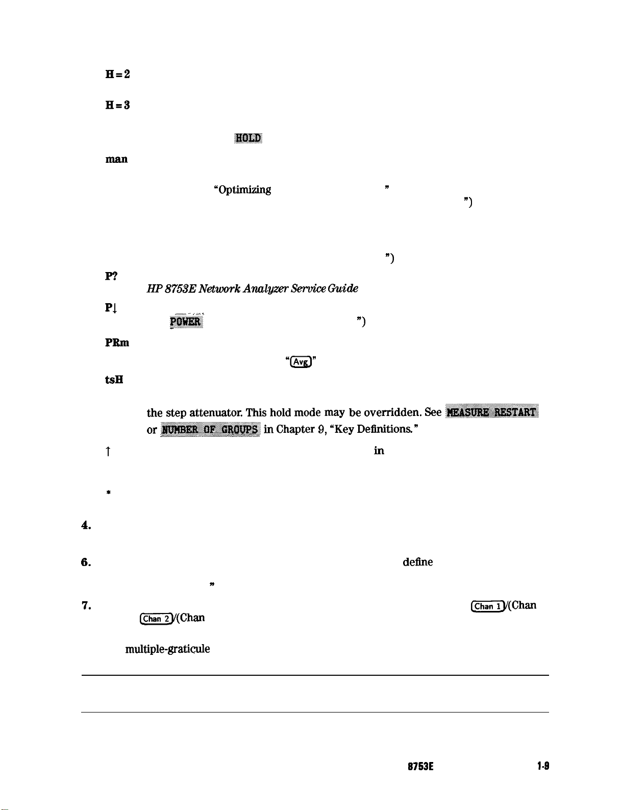
H=2

Harmonic mode is on, and the second harmonic is being measured (harmonics Option 002 only). (See “Analyzer Options Available” later in this chapter.)

H=3

Hld

PC?

PRltl

Smo

tsH

Harmonic mode is on, and the third harmonic is being measured (harmonics Option 002 only). (See “Analyzer Options Available” later in this chapter.)

Hold sweep. (See

:@&I$

in Chapter 9, “Key Definitions.“)

Waiting for manual trigger.

Power meter calibration is on. (For power meter calibration procedures, refer to Chapter 5,

“Optimlzmg

Measurement Results. n For power meter calibration

theory, refer to Chapter 6, “Application and Operation Concepts. “) The analyzer’s source could not be set to the desired level, following a power

meter calibration. (For power meter calibration procedures, refer to Chapter 5,

“Optimizing Measurement Results.” For power meter calibration theory, refer to

Chapter 6, “Application and Operation Concepts

“)

Source power is unleveled at start or stop of sweep. (Refer to the

8753E Network

Source power has been automatically set to

.i............/

..i ..i i

(See

J%I@

in Chapter 9, “Key Definitions. “)

An.uZgm

Semrice Guide

for troubleshooting.)

minimum, due to receiver overload.

Power range is in manual mode. Trace smoothing is on. (See

“0”

in Chapter 9, “Key Dellnitions.“) Indicates that the test set hold mode is engaged. That is, a mode of operation is selected which would cause repeated switching of

the step attenuator. This hold mode may be overridden. See ~~~~~~~~~

. . . . . .

or ~~~~~~~~~~~

) _,_/,,,/,,

.:.:.:,:.:.:.:.

;.;..~,.~,.~,.~.~~;~,:~:~~~~;.:~~:.:;~~~~~~~~:.:~.,.~:

/,,,. :.:.,.:.:.:

.,,,. :.:.: .,,,.... :.:-_

Chapter 9, “Key Definitions”

Fast sweep indicator. This symbol is displayed

the status notation block when

sweep time is less than 1.0 second. When sweep time is greater than 1.0 second,

this symbol moves along the displayed trace.

Source parameters changed: measured data in doubt until a complete fresh sweep has been taken.

Active

Message

Title.

Entry

This is a descriptive alphanumeric string title that you

Area.

This displays the active function and its current value.

Area.

This displays prompts or error messages.

define

and enter through

an attached keyboard or as described in Chapter 4, “Printing, Plotting, and Saving

Measurement Results.

Active Channel. This

3) and

w(Chan

is the label for the active channel, selected with the

@Gily(Chan

4) keys. If multiple channels are overlaid, the labels will appear in

this area. The active channel is denoted by a rectangle around the channel number. For

multiple-graticule

displays, the channel information labels will be in the same relative

position for each graticule.

Note

The label of the active channel is enclosed in a rectangle to differentiate it from inactive channels.

6753E

Description and Options

l-6

8. Measured Input(s).

This shows the S-parameter, input, or ratio of inputs currently measured, as selected display memory status.

using

the

LMeas)

key. Also indicated in this area is the current

Format.

10.

Scale/Div. This is the scale that you selected using the

This is the display format that you selected using the (Format] key.

(Gig)

key, in units appropriate

to the current measurement.

11. Reference Level.

in polar formats, whichever you selected using the

This value is the reference line in Cartesian formats or the outer circle

&XiGf]

key. The reference level is

also indicated by a small triangle adjacent to the graticule, at the left for channel 1 and at

the right for channel 2 in Cartesian formats.

12.

Marker Values.

These are the values of the active marker, in units appropriate to the

current measurement. (Refer to “Using Analyzer Display Markers” in Chapter 2, “Making

Measurements.

13. Marker Stats, Bandwidth.

calculates when you access the menus with the

“)

These are statistical marker values that the analyzer

@GZZ&)

key. (Refer to “Using Analyzer

Display Markers” in Chapter 2, “Making Measurements.“)

14.

Softkey

Labels. These menu labels

redellne

the function of the

softkeys

that are located

to the right of the analyzer display.

15. Pass

Fail.

Duriug

limit testing, the result will be annunciated as PASS if the limits are not

exceeded, and FAIL if any points exceed the limits.

l-10

HP 8753E Description and Options

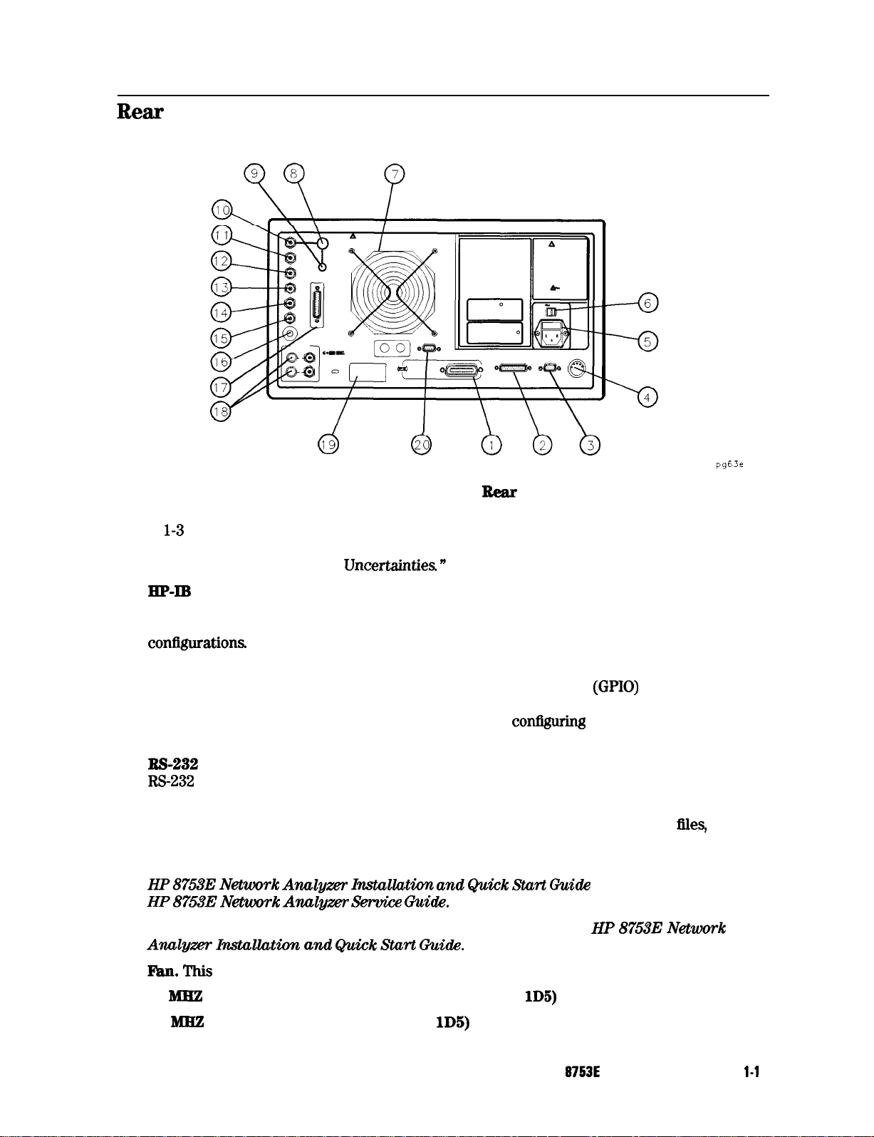
Rear

Panel Features and Connectors

Figure 1-3. HP 8753E Bear Panel

pg63e

Figure Requirements for input signals to the rear panel connectors are provided in Chapter 7,

“Specifications and Measurement

l-3

illustrates the features and connectors of the rear panel, described below.

Uncertanuies

HP-Ill connector. This allows you to connect the analyzer to an external controller,

compatible peripherals, and other instruments for an automated system. Refer to the

“Compatible Peripherals” chapter in this document for HP-IB information, limitations, and

coniigurations

PARALLEL interface.

a parallel input. Also included, is a general purpose input/output control eight output bits and read five input bits through test sequencing. Refer to the “Compatible Peripherals” chapter for information on

to “Application and Operation Concepts” for information on GPIO.

RS-232 W-232 (serial) input.

KEYBOARD input (mini-DIN). This

keyboard. This provides a more convenient means to enter a title for storage ties, as well as substitute for the analyzer’s front panel keyboard.

Power cord receptacle, with fuse.

HP87533 Network HP 87533 Network Analps- Seruice Guide.

Line voltage selector switch.

Analyzer Installation and Quick Start Guide.

interface

This connector allows the analyzer to output to a peripheral with

This connector allows the analyzer to output to a peripheral with an

connector allows you to connect an external

For information on replacing the fuse, refer to the

Anulgzer

Instullution

For more information refer to the

con@uing

and

Quick Start Guide or the

(GPIO)

a peripheral. Also refer

bus that can

87533 Network

l%.n. This

PRECISION REFERENCE OUTPUT. (Option lD5)

MHZ

REFERENCE ADJUST. (Option

fan provides forced-air cooling for the analyzer.

lD5)

8753E

Description and Options

l-1

10.

EXTERNAL

BEF‘ElUINCE INPUT. connector. This allows for a frequency reference signal

input that can phase lock the analyzer to an external frequency standard for increased frequency accuracy.

The analyzer automatically enables the external frequency reference feature when a signal is connected to this input. When the signal is removed, the analyzer automatically switches back to its internal frequency reference.

11.

AUXILIABY INPUT

connector.

This allows for a dc or ac voltage input from an external signal source, such as a detector or function generator, which you can then measure, using the S-parameter menu. (You can also use this connector as an analog output in service routines, as described in the service manual.)

12.

EXTERNAL AM connector.

applied to the

ALC

circuitry of the analyzer’s source. This input analog signal amplitude

This allows for an external analog signal input that is

modulates the RF output signal.

13.

EXTERNAL

TI’L-compatible

external through

14.

TEST SEQUENCE.

to be high or low, or pulse (10

TRIGGER

connector.

This allows connection of an external negative-going

signal that will trigger a measurement sweep. The trigger can be set to

softkey

functions.

This outputs a

‘ITL

pseconds)

signal that can be programmed in a test sequence

high or low at the end of a sweep for robotic part

handler interface.

15.

LIMIT TEST.

This outputs a

TI’L

signal of the limit test results as follows:

n Pass: TTLhigh

Fail:

ITLlow

MEASURB EJZSTART.

16.

This allows the connection of an optional

fo,ot.

switch. Using the

foot sMtch m duplicate the key sequence 1Meas) :~~~,~,~~~~~~~~.

TEST SET

17.

analyzer to an HP

INTEECONNECC.

85046A/B

This allows you

85047A

to connect an HP 8763E Option 011

S-parameter test set using the interconnect cable supplied with the test set. The S-parameter test set is then fully controlled by the analyzer.

BIAS INPUTS AND FUSES. These

18.

port 2. The fuses (1 A, 125

Serial number plate.

19. EXTERNAL

20.

MONITOB:

The serial number of the instrument is located on this plate.

V) protect the port 1 and port 2 bias lines

VGA.

connectors bias devices connected to port 1 and

VGA output connector provides analog red, green, and blue

video signals which can drive a VGA monitor.

l-12

HP8753EDesoriptionandOptions

Analyzer Options Available

Option

Option lD5 offers

lD6,

High Stability Frequency Reference

kO.05

ppm temperature stability from 0 to 60 OC (referenced to 25

“C).

Option 002, Harmonic Mode

Provides measurement of second or third harmonics of the test device’s fundamental output signal. Frequency and power sweep are supported in this mode. Harmonic frequencies can be measured up to the maximum frequency of the receiver. However, the fundamental frequency may not be lower than 16

Option 006, 6

Option 006 extends the maximum source and receiver frequency of the analyzer to 6

GHz

MHz.

Operation

GHz.

Option 010, Time Domain

This option displays the time domain response of a network by computing the inverse Fourier transform of the frequency domain response. It shows the response of a test device as a function of time or distance. Displaying the reflection coefficient of a network versus time determines the magnitude and location of each discontinuity. Displaying the transmission coefficient of a network versus time determines the characteristics of individual transmission paths. Time domain operation retains all accuracy inherent with the correction that is active in the frequency domain. The time domain capability is useful for the design and characterization of such devices as SAW

iilters,

SAW delay lines, RF cables, and RF antennas.

Option 011, Receiver Configuration

Option 011 allows front panel access to the R, A, and B samplers and receivers. The transfer

switch, couplers, and bias tees have been removed. Therefore, external accessories are

required to make most measurements.

Option

Option 075

Option

This option removes the built-in flat panel display, allowing measurement results to be viewed with an external monitor only.

Option

Option mount the instrument, with handles detached, in an equipment rack with 482.6 mm (19 inches) horizontal spacing.

076, 768

offers 75 ohm impedance bridges with type-N test port connectors.

lDT,

lCM,

1CM

is a rack mount kit containing a pair of flanges and the necessary hardware to

Impedance

Delete Display

Rack Mount Flange Kit Without Handles

HP 8753E Description and Options

1-13

Option

lCP,

Rack Mount Flange Kit With Handles

Option mount the instrument with handles attached in an equipment rack with 482.6 mm (19 inches) spacing.

1CP

is a rack mount kit containing a pair of flanges and the necessary hardware to

Service and Support Options

Hewlett-Packards offers many repair and calibration options for your analyzer. Contact the nearest Hewlett-Packard sales or service office for information on options available for your

analyzer.

l-14 HP

8753EDescriptionand

Options

Differences among the HP 8753 Network Analyzers

lhble

l-l. Comparing the

J3P 8753AIBKYD

Feature

Fully integrated measurement system (built-in test

s&J

lbst

port power Auto/manual power m selecting Port power Internal disk drive Precision frequency reference (Option Frequency range - low end Ext. freq. range to 6

750 system impedance (Option 075)

TRL*/LRM*

Power meter calibration Interpolated error correction Max. error corrected measurement points Segmented error correction in freq. list mode Color

CXT

Test sequencing Automatic sweep

JSxkrnal

Tuned receiver mode Printer/plotter

Harmonic measurements (Option 002) Frequency offset mode (mixer measurements) dc Interfaces:

keyboard

User-detlned

Non-volatile memory

Dvnamic~

Real

source capability

bias

to test device

3OkHzto3GHz 3GHzto6GHz

time clock

300

t For this network $ OOdBfrom30kHzto5OkHz, lOOdBfrom3OOkHzto16MHz

rfmge (dDm)

coupliug/uncoupling

GHz

(Option 006)

correction

time

bufPer

RS-232,

parallel, and DIN

preset

kHz

to 3

GHz,

without Option 006,

analyzel;

lD5)

the feature is dependent on the test

8763A

No 1 No

No No No

300 kHz

t No No No

801

No No No No No No No No No

t No

No 1 No

a30kHzto6GHz,wii

8753B

No No No

300 kHz

Yes

YeS

1001

No Yes Yes

YeS

Yes

8758C

8768D

Ye8

8758D

z-t++

3oolcHz

3okHz

Yes

No Yes Yes

1001

Yes YW

YeS

Yes

YeS Ye8

Yes Yes

Ye8

Yes Yes Yes Yes

YeS

1601

Ye8

Yes

YeS YeS YeS

Yes

YeS

?fjFpjc

Option 006

set

being used.

3OBOO

512

1OOdB

110 dB

Opt

011

No No

Ye8

Yes

kHz’

YeS

Yes

YeS

1601

YeS

Yes Yes Yes Yes

Ye8

Yes Yes

YeS

Yes

Kbytes

Ye8

8753E

Description and Options

l-15

‘able

1-2. Comparing the HP

8753D

and HP 8753E

300

lcHz

to 3

GHz,

without option 006, or 30

For this network

$ QOdBfrom30kHzto6OkHz, lOOdBfrom3OOkHzto16MHz

l-1

6763E

Description and Options

analyze5

the feature is dependent on the test set being used.

lcHz

to 6

GHz,

with Option 006

Making Measurements

This Chapter contains the following example procedures for making measurements or using particular functions:

Basic measurement sequence and example

0 Setting frequency range 0 Setting source power

Analyzer display functions

Four-Parameter Display Mode

Analyzer marker functions

Magnitude and insertion phase response

Electrical length and phase distortion

Deviation from linear phase

Group delay

Limit testing

Gain compression

Gain and reverse isolation

Measurements using the swept list mode

Tuned Receiver Mode

Test

sequencing

Measuring Swept Harmonics

Time domain

Transmission response

Reflection response

Non-coaxial measurements

Where to Look for More Information

Additional information about many of the topics discussed following areas:

Chapter 4, “Printing, Plotting, and Saving Measurement Results,” contains instructions for saving to disk or the analyzer internal memory, and printing and plotting displayed measurements.

Chapter 5, “Optimizing Measurement Results,” describes techniques and functions for achieving the best measurement results

Chapter 6, “Application and Operation Concepts, about many applications and analyzer operation.

Chapter 9, “Key Definitions,” describes all the front panel keys and softkeys.

Chapter 11, “Compatible Peripherals,” lists measurement and system accessories, and other applicable equipment compatible with the analyzer.

this Chapter is located in the

contains explanatory-style information

Making Measurements

2-l

Principles of Microwave Connector Care

Proper connector care and connection techniques are critical for accurate, repeatable measurements.

Refer to the calibration kit documentation for connector care information. Prior to making connections to the network analyzer, carefully review the information about inspecting, cleaning and gaging connectors.

Haying good connector care and connection techniques extends the life of these devices. In

addition, you obtain the most accurate measurements. This type of information is typically located in Chapter 3 of the calibration kit manuals. For additional connector care instruction, contact your local Hewlett-Packard Sales and Service

Office about course numbers HP See the following table for quick reference tips about connector care.

8505OA

24A

and HP

8505OA

24D.

‘lhble 2-l.

Extend sleeve or

Use plastic end-caps during storage

Inspect Look for metal particles, scratches, and dents

Clean connector threads

Use the correct Use correct end of calibration block Gage aU connectors before

alI

se isopropyl alcohol

conuector

connectors carefully

Connector Care Quick Reference

nut

Ilrst

use

Set connectors contact-end down

Get liquid into plastic support beads

Align

connectms

Make preliminary connection lightly

Turn only the connector nut

Use a torque wrench for

2-2

Making Measurements

carefully

Making connections

Do Not Apply bending force to connection Over tighten preliminary connection Twist or screw any connection

fInal

connect Tighten past torque wrench “break” point

Basic Measurement Sequence and Example

Basic Measurement Sequence

There are five basic steps when you are making a measurement.

1. Connect the device under test and any required test equipment.

Caution

Damage may result to the device under test if it is sensitive to the analyzer’s default output power level.

avoid damaging a sensitive DUT, be sure to set

the output power appropriately before connecting the dut to the analyzer.

2. Choose the measurement parameters.

3. Perform and apply the appropriate error-correction.

Measure the device under test.

5. Output the measurement results.

Basic Measurement Example

This example procedure shows you how to measure the transmission response of a

Glter.

bandpass

Step 1. Connect the device under test and any required test equipment.

1. Make the connections as shown in Figure

2-l.

NETWORK

ANALYZER

DEVICE

UNDER TEST

Figure 2-1. Basic Measurement Setup

Step 2. Choose the measurement parameters.

2. Press

Setting the Frequency Range.

3. To set the center frequency to 134 MHz, press:

To set preset to “Factory Preset,

press:

[centerl(TzJ(iiiJg

Meking

Measurements 23

pg6’e

‘lb

set the span to 30 MHz, press:

&g(ziJm

Note

Setting the Source Power.

change the power level to -5

Note

Setting the Measurement.

‘Ib

change the number of measurement data points to 101, press:

7. To select the transmission measurement, press:

8. To view the data trace, press:

You could also press the @ and limits as start frequency and stop frequency values

dRm,

press:

You could also press power ranges to keep the power setting within the

~~~~.~~~~~~~~ ~~~~~~:~,~~~~~

&TJ

keys and enter the frequency range

/ _

and select

deGned

range.

one

of the

Step 3.

9. Refer to the

10. To save the instrument state and error-correction in the analyzer internal memory, press:

Perform

measurement errors.

and apply the appropriate error-correction.

“OpUmizing

Measurement Results” Chapter for procedures on correcting

24 Making Measurements

Caution

Step

Measure the device under test.

11. Replace any standard used for error-correction with the device under test.

Do not mistake the Iine switch for the disk eject button. See the figure below. If the Iine switch is mistakenly pushed, the instrument losing ah settings and data that have not been saved.

DISK EJECT

BUTTON 1

LINE SWITCH’

wiIi

be turned off,

12. To measure the insertion loss of the

m(i5iJm

Step 6.

13.

Output

‘Ib

create a hardcopy of the measurement results, press:

Refer to Chapter 4, ‘Printing, Plotting, and Saving Measurement Results,” for procedures on how to define a print, plot, or save. For information on configuring a peripheral, refer to Chapter 11, “Compatible Peripherals.

the measurement results.

bandpass

filter, press:

Making Measurements

2-5

Using the Display Functions

View Both Primary Measurement Channels

In some cases, you may want to view more than one measured parameter at a time.

Simultaneous gain and phase measurements for example, are useful in evaluating stability in negative feedback amplifiers. You can easily make such measurements using the dual channel display.

1. To see channels 1 and 2 in the same grid, press:

2* ‘lb

view the measurements on separate graticules, press: Set

analyzer shows channel 1 on the upper half of the display

of the display. The analyzer also defaults to measuring

Sll

Figure 2-3. Example

Dua.l

Channel With Split Display On

” ,.:s’<$$:.<

~~~~~~~~‘~~~~~

an~~~~~~~~n

2X.

The

the lower half

on channel 1 and &I on channel

~000027

2-6

Making Measurements

3. To return to a single-graticule display, press:

~~~~~~~;.,~~~~~~~,,,

.,.. ..,......., ,,,,,,,,...........,.

..:.

. . .

. . . . . . . . .

$8,

. . . . .

..A .i

. . . . . . . . . .

..s..........i

Note

Save a Data Trace to the Display Memory

You can control the stimulus functions of the two channels independent of each

other, by pressing LMenu) &@&&

.kE

@FE

../

_ ., _ ., ,.

Press

(j) ~~~~~~~~~~

the active channel. The data trace is now also the memory trace. You can use a memory trace for subsequent math

manipulations.

View the Measurement Data and Memory Trace

The analyzer default setting shows you the current measurement data for the active channel.

1. To view a data trace that you have already stored to the active channel memory, press:

p&q--

i~~~~.~

..,........,

..:.......s

/:.i

. . . . . . . . . ..A.. ~..~...~

This is the only memory display mode where you can change the smoothing and gating of the memory trace.

‘lb

view both the memory trace and the current measurement data trace, press:

to store the current active measurement data in the memory of

Making Measurements

2-7

Divide Measurement Data by the Memory Trace

You can use this feature for ratio comparison of two traces, for example, measurements of gain or attenuation.

1. You must have already stored a data trace to the active channel memory, as described in Save a Data Trace to the Display Memory.”

2. Press (Display) The analyzer normalizes the data to the memory, and shows the results

..“’ :.

~~~~~~

il....:i.i

to divide the data by the memory.

.:..

“To

To Subtract the Memory Trace from the Measurement Data Trace

You can use this feature for storing a measured vector error, for example, directivity. Then, you can later subtract it from the device measurement.

1. You must have already stored a data trace to the active channel memory, as described in Save a Data Trace to the Display Memory.

press (jj

The analyzer performs a vector subtraction on the complex data.

‘RI

Ratio Measurements in Channel 1 and 2

You may want to use this feature when making amplifier measurements to produce a trace that represents gain compression. For example, with the channels uncoupled, you can increase the power for channel 2 while channel 1 remains unchanged. This will allow you to observe the gain compression on channel 2.

1. Press lMenJ ~~~~~~~~~~~~ to mcouple the c.,annels.

~~~ar~~~~, to subtract the memory from the measurement

;;;;A.::..:

..:.....,...:....

. . .

2..

,,.,.,....;

.,.,,.,.,.,.,.....,.,..,.;

. . . . . . . . . . . . .

..i ...........

. . .

.::

.: i.:::........;.;~

i... . . . . . . .

.:::

i.......i

.A..

data.

“‘lb

2. Make sure that both channels must have the same number of points.

a. press (~,

on the analyzer display.

b. Press

3. Press ~~isp,ay, ~~~

channel 2 data array. This ratio is applied to the complex data.

4. Refer to Chapter “Measuring Gain Compression” for the procedure on identifying the 1 compression point.

@iZZ) [Menu_)

the channel 1 setting.

[=, ~~~~~~~~~~

. . . .

..I.............................,.,.,..:

.,., p ,. ,,,,. ‘I .& ...:.,:::::~

~~~~~~~~~:~~~~~ and enter the same value that you observed for

,,a...

. . .

. . . . . . .

i ,......

.::::.:..

.A.................

~~~.~~.

. . . . .

.:.,.;.;.,;;;..;;;.i

~~~~~~~,~~~~

,.;;

. . . . . . . .

;;: .A....

LL.;.

;. . . . . .

. .

..A T.T

. . .

.._....

. . . . . . . . . . . . . . . . .

L.~~~~.,~...,..,~~~ .............i

and notice the number of points setting, shown

....

..:::.:

...: ,:,:, :-;,:::::.:

. . ....

.::::::

to ratio channels l and 2, and put the results in the

2-8

Making Measurements

Title the Active Channel Display

. ii

1. press (misplay)

press,~~~~~~~

>> ;.:..:.<:..

If you have a DIN keyboard attached to the analyzer, type the title you want from the keyboard. Then press

&&:: $&$ to access the title menu.

,... ..: i;: //

..c c......

.!;;:.;;::...iii

~.~./i

enter the title you want for your measurement

(WI

to enter the title into the analyzer. You can enter a title

&splay.

that has a maximum of 50 characters. (For more information on using a keyboard with the analyzer, refer to “Keyboards” in Chapter 11, “Compatible Peripherals.“)

If you do not have a DIN keyboard attached to the analyzer, enter the title from the analyzer front panel.

a. Turn the front panel knob to move the arrow pointer to the

first

character of the title.

c. Repeat the previous two steps to enter the rest of the characters in your title. You can

enter a title that has a maximum of 50 characters.

‘...:.:.:.:.:.....“”

. . . . . .

.,.,..,.,.,.

d. Press

.,. /

~@I@#$

to complete the title entry.

.:...

III CENTER

Figure 2-4. Example of a Display Title

135 BBB wad M!iz

Ill

5PRN

IllI

58 888

“HZ

aw000029

Making Measurements

2-8

The display will appear as shown in

F’igure

2-5. Channel 1 is in the upper left quadrant of the display, channel 2 is in the upper right quadrant, and channel 3 is in the lower half of the display.

LOG

dB/

CHl

LOG

Sll

CENTR 134.000 MHz

CH3

s12

REF -2

SPFIN

45.000 MHz

dB/REF

-50

17 Ssp 1998

CH2

LOG

521

Cot-

START 111.500 MHz STOP 156.500 MHz

dB/

11:13:31

REF

-50

I I I

DUAL

CHAN

ON off

AUX

CHAN

ON off

PARAM

DISPLAYS

SPLIT DISP

CHANNEL

POSITION

CENTER 134.000 000 MHz

Figure 2-5.

3-Channel

SPAN

Display

45000

RETURN

000 MHz

Making Measurements 2-11

This enables channel 4 and the screen now displays four separate grids as shown in Channel 4 is in the lower-right quadrant of the screen.

Figure

2-6.

CHI

LOG

-31

PRnE

CENTR 134.000

CH3

LOG 10

s12

. 5

dB/

MHz SPFIN

dB/

REF

-2

45.000 MHz

REF -50 dB

2 Sep 1998

CH2

LOG

s21

PRm

CENTR 134.000 MHz SPAN 45000

% LoG

14:is:

dB/

REF -50

dB/

REF -3 dB

MHz

DUAL CHAN

ON off

AUX CHAN

ON off

PARAM

DISPLAYS

SPLIT DISP

CHANNEL

POSITION

rll

CENTR 134.000 MHz SPAN 45.000 MHz CENTR 134.000 MHz SPAN

Activate and

I I

Co&lgure

I I

Figure 2-6.

4-Channel

the Auxilkry Channels

Display

45000

RETURN

MHz

This procedure continues from the previous procedure.

10. Press

(j-1

Observe that the amber LED adjacent to the

again.

@iGTj hardkey

is flashing. This indicates that

channel 4 is now active and can be configured.

........

11. &-ess w

...

:~~:~...;; ................................

Markers 1 and 2 appear on moves marker 2 on

.............................

~~~~~.,

.::.~~.~~~~~~~:~

all

...................................................................

..........

all

four channel traces. Rotating the front panel control knob

four channel traces. Note that the active function, in this case the

marker frequency, is the same color and in the same grid as the active channel (channel 4.)

12. Press

@GiJ.

Observe that the LED adjacent to

@GTj

is constantly lit, indicating channel 1 is active.

2-l 2 Making Measurements

13.

Press (Ghan] again.

Observe that the LED is flashing, indicating that channel 3 is active.

14. Rotate the front panel control knob and notice that marker 2 still moves on all four channel traces.

15. To independently control the channel markers:

**,, .:.

Press (Marker)

.::.

‘~~~~~~::::.~~,

. .

. .../ i

. . . . .

i......;.;;;;

.......... . .

i.i

....

. . .

..i.. i/......ii

set

~jQ#$JR&~~-

to UNCOUPLED.

Rotate the front panel control knob. Marker 2 moves only on the channel 3 trace.

Once made active, a channel can be variables except stimulus. For example, Smith chart by pressing

@GZ) $#$Z~B&KX..

conhgured

;

;;;

once~channel3

. . . . . .

.a:

;:., ,.:.:...:..

.._...,..........................

T .....

. . . . . . . . . .

independently of the other channels in most

is active, you can change its format to a

Quick Four-Parameter Display

.,. . . . . . . . . . . .

The ~~~.~~~~~~~~~:,;

>:;:,I; 1.:. $,>,;> ,,.:.::.,;,.,..:. :.: . . . . :.:.:.:.::..~:.~~~~~~::~~:.:.:.:.~~:::,~:.;,:.:.,.:.:.:.:.:.:.,.:

parameter assignments.

.,., .;:.. ,.

Press

. . . . . ._:...

~~~~~

For more information about the

and Operation Concepts.

.;. ,.., .,.

..::

.,.....,.,.......

. . . . . .

menu gives you a choice of standard

,,,,,,i: .,., <:...

in place of step 6.

~~~~~~~~~~~~~

channel

conmations

and

menu, refer to chapter 6, “Application

Characterizing a Duplexer

The following example demonstrates how to characterize a duplexer. This measurement utilizes four-parameter display mode.

A duplexer’s three ports are:

Transmit

Receive (Rx)

Antenna (Ant)

(TX)

There are two signal paths through a duplexer: from Tx to Ant, and from Ant to Rx. The two signal paths are offset in frequency from each other and have the antenna (Ant) port in common.

This example displays the tr

ansmission

(TX-to-Ant and Ant-to-Rx) characteristics of the duplexer in the top half of the display, and the reflection characteristics (Tx and Rx ports) in the bottom half. Therefore, the stimulus is set up so that it is centered midway between the transmit and receive frequencies of the duplexer, and the span is set to cover the combined receive and transmit frequencies.

Other display configurations are possible. For example, the display can be configured so that the transmission and reflection of the

TX-Ant

path is shown in the top half of the display, and

the transmission and reflection of the Ant-Rx path is shown in the bottom half of the display.

3-port

device, in this case a

Making

Meesurements 2-13

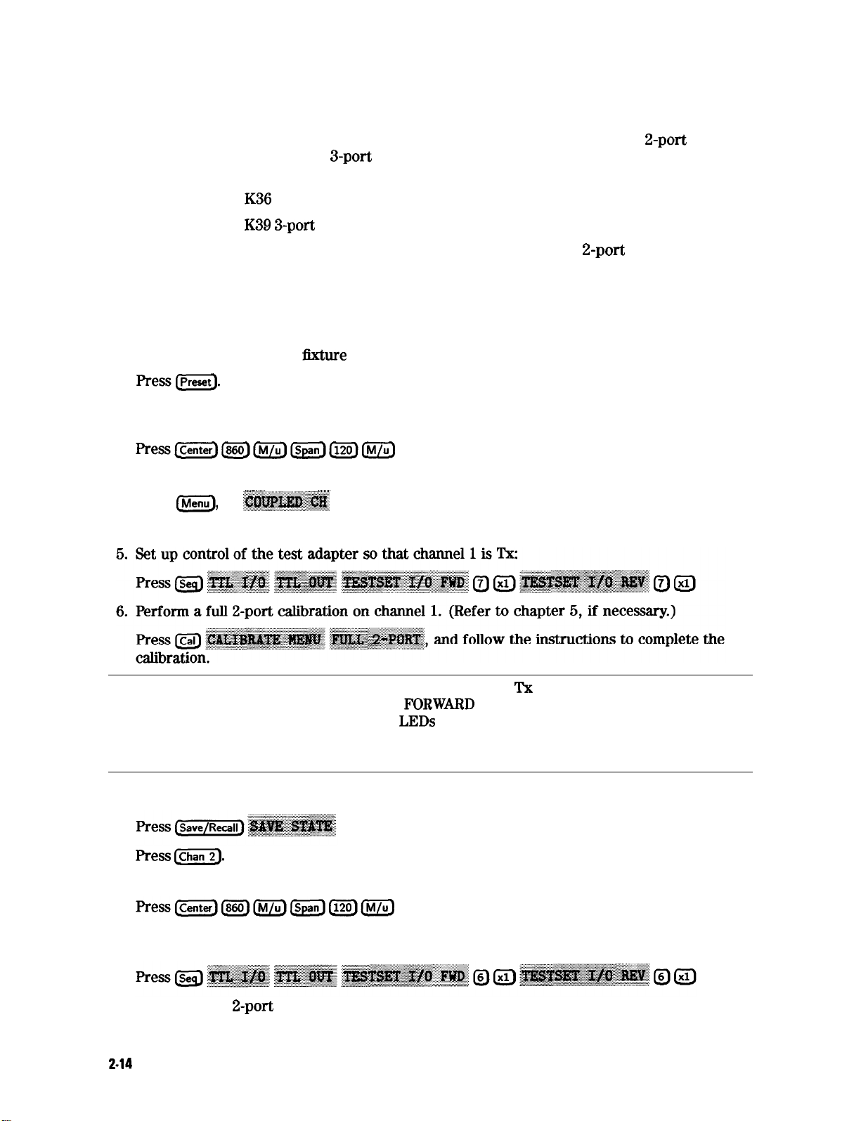
Required Equipment

Characterizing a duplexer requires that the test signals between the analyzer (a 2-port instrument) and the duplexer (a 3-port device) are routed correctly. This example uses one of the following adapters to perform this function:

HP 8753E Option

K36

duplexer test adapter

K39 3-port

test adapter

You must also have a set of calibration standards for performing a full 2-port calibration on your test set up.

Procedure for Characterizing a Duplexer

1. Connect the test adapter to the analyzer according to the instructions for your particular model. Connect any test

Press=.

3. Set up the stimulus parameters for channel 1 (center/span frequencies, power level, IF bandwidth). This example uses a span of 120 MHz centered at 860 MHz.

PressIcenter)@ZJLM/U)CSpan)(EJLM/U)

llxture

or cables to the duplexer test adapter.

4. Uncouple the primary channels from each other:

.,; .,.... .,.,.. ,,...:...

. . . . . . . . . . . . . . . . . . . . .

Press

m),

set

~~~~~~

.........

to OFF.

(This is necessary in order to set the test set I/O independently for each channel.)

Note

Make sure you connect the standards to the TX port of the test adapter (or a cable attached to it) for the FORWBD calibration and to the Ant port for the REVERSE calibration. The

LEDs

on the test adapter indicate the active ports: a brightly lit LED indicates the source port; a dimly lit port indicates the input port; an unlit LED indicates no connection.

When the calibration has been completed, save the instrument state:

8.9.Press

@iLZiJ

Set up channel 2 for the same stimulus parameters as channel 1.

Set up control of the test adapter so that channel 2 is measuring the receive path of the

10. duplexer: (Uncoupling the channels allows a different calibration for each signal path.)

Perform a full

11.

2.14

Making Measurements

2-port calibration on channel 2:

..:::c. ..:.:.:.: “)

.:.:.:.:..

,. ,.,..: _ _

Press Lcal] .~~~~~~;~~~~.~. &@f& &+%Rf~

.,.

::.:.

Note

Make sure you connect the calibration standards to the Rx port of the test

adapter (or a cable attached to it) for the FORWARD calibration, and the

Antenna port for the REVERSE calibration.

12. When the calibration has been completed, save this state in the analyzer:

13. Connect the DUT to the test adapter.

14. Enable both auxiliary channels 3 and 4: Press (Display)

..;;..~.....~._;

..z. / :+

. . . . .

. .

..i >n;;.~

,;..:.:;:;..::::

~7::

..:. .:’

set

..;p

~~~~~~~ ,;f@%JR~

. ..a

ii..;;;;; ii

x.... . . . . .

.A....

. .

..A

AI& ~:~I$&&

,,,,....

. . . . . . . . . . . . . . . . . . . . L.

to ON, press

@GiJ

and set

. .

..::::

&J@$HA#

. . . . . . . . .

:..:,;:

“,:,::...:...:.:.:.:..,,,::

ON.

15. Set up a two-graticule, four-channel display:

16. Set the measurement parameters (channel 1 should be active):

a. fiess IMeas] ~~~~

This is the transmission of the

b. Press

@iGil

.:.. ..,.,.:,..,,

. . .

.,.:::::

‘k-to-Ant

path.

,*;.................,.

to activate channel 3, press

@$g;.

,,.

This is the reflection at the TX port.

Press c-1

f&&g;

This is the transmission of the Ant-to-Rx path.

d. F%ess @G-T)

to activate channel 4, press

This is the reflection at the Rx port.

The display will be similar to Figure 2-7.

i /

...*.

$%$.‘.

Making Measurements

2-15

CHl CH2

s21 s12

LO8

LOG

10 10

dB/REF dB/REF

-40

dB dB

5 Au9 1998

13:10:11

Ref 1: FWD

Sll <A/R)

Trans: FWD

521 <B/R)

PRm Cot-

10 10

dB/REF dB.‘REF

0 0

dB dB

Trans: REV

S12

<FI.‘R)

Ref 1: REV

S22 (B/R)

ANALOG IN Aux Input

CONVERSION

COFFI

CHl/CH3 CHZ/CH4

CENTER CENTER

860.000 000

MHz MHz

120.000 000

SPAN

120.000 000

SPAN

MHz MHz

Figure 2-7. Duplexer Measurement

Normally, a

2-port

calibration requires a forward and reverse sweep to

Cnish

before updating the displayed trace. For faster tuning, it is possible to set the number of sweeps for the active display

(Sll

and

S21

for channel 1 in this case) to update more often than the unused parameters. In this example we choose 8 updates of the forward parameters to 1 update of the reverse in channel 1, and 8 updates of the reverse to 1 update of the forward in channel 2 (where the active parameters are

press I-1 Press c-1 (77) ~~~~~~~~~~

Lj)

~~~~~~~~

.._..............................-...-...-....................

.._.....................................-.........

S22

::..

_ __ . . . . .

and

S12).

.....

~~~~~ :;~~~~~~~~

_.........

_...

~~~~~.~~ ‘~~~~~~

..^..

i..~.;;Li.>:.:

..:::::..

.,. ,...; . . . . . . . ;;;; . . . . . . . . . . . . . . . . . i...~.,..i

. . . . . . . . . . . . . . . . . . . . . . . . . . . . . . . . . . . . . SW....;;;...:....

...,

../

@J). (QJ1.

. . . . . . . . . . . . . . . . . . . . . . . . . . . . .

..A. ii

.../... .>.~.,.W_,.

INPUT

PORTS

2-16

Making Measurements

Using Analyzer Display Markers

The analyzer markers provide numerical readout of trace data. You can control the marker search, the statistical functions, and the capability for quickly changing stimulus parameters with markers, from the

Markers have a stimulus value (the x-axis value in a Cartesian format) and a response value (the y-axis value in a Cartesian format). In a polar or Smith chart format, the second part of a complex data pair is also provided as an auxiliary response value. When you switch on a marker, and no other function is active, the analyzer shows the marker stimulus value in the active entry area. You can control the marker with the front panel knob, the step keys, or the front panel numeric keypad.

If you activate both data and memory traces, the marker values apply to the data trace.

If you activate only the memory trace, the marker values apply to the memory trace.

If you activate a memory math function (data/memory or data-memory), the marker values

apply to the trace resulting from the memory math function.

(jMarker)

key.

Use Continuous and Discrete Markers

The analyzer can either place markers on discrete measured points, or move the markers continuously along a trace by interpolating the data value between measured points

Press

@ilXZG) ~~~~~~~~

_ _ _ ,.__

..;~.‘. .~

.;y

. . . . . .

and select one of the following choices:

conveniently obtain round numbers for the stimulus value.

C.,oose ~~~~~~~~

;

you wmt the andyzer to place mxkers ody on measured

trace points determined by the stimulus settings. This may be the best mode to use with automated testing, using a computer or test sequencing because the analyzer does not interpolate between measured points.

; . ...% /:.:,,

..:...:. ..:. ..:. ...

.:~:.:~:~:~:~:~:~:.

. . .

;~~#$Z&$gm

..~..::::.~...:::::....:..;:::: . . . . ..““.;“; ../)

&so affect maker search ad positioning

Note

using ;m”

,. _ .,. _. . ,..........

2: . . . . . s.; . .

..A.. .>;

. . . . . . . .. . . . . . . .::::: ::.... ::..::;.../ii . . . . .zw;;...i . . ..A I .A.. .i . . . . . ..v >;.:: .A.. ~.......;;...i:..:.

functions when the value entered in a search or positioning function does not

exist as a measurement point.

Making Measurements

2-17

Activate Display Markers

switch on marker 1 and make it the active marker, press:

(Iizzia .~..~~~~~

The active marker appears on the analyzer display as V. The active marker stimulus value is displayed in the active entry area. You can modify the stimulus value of the active marker, using the front panel knob or numerical keypad. All of the marker response and stimulus values are displayed in the upper right comer of the display.

Figure 2-8. Active Marker Control Example

To switch on the corresponding marker and make it the active marker, press:

,,....,, ,,,,,,.,.,,,,

ihk.>,I .:.. .::::.w..::::::;:::::::::::::.~:;&::

All of the markers, other than the active marker, become inactive and are represented on the analyzer display as A.

~~~:

?cz;

‘. :

.:...:~~~~~~~~~:::.:----.~~~~~~~

..i: 9

~~~

.:*:~~<;~<:

Figure

“7

or ~~~~~

..,_.. :u::..p.*~~~

2-9. Active and Inactive

.. ,_,, ::*:,; ,,,, :~...i.~.~~v::~. ,. /

Markers

Example

‘Ib

switch off all of the markers, press:

.._; _/ ., _...

.,..,

/ _

~~~,

2-l 8

.,.... _

.,. .,.,.,.,. . . . . .

. .

i..;,; ...i..

Making Measurements

!tb

Move Marker Information off of the Grids

If marker information obscures the display traces, you can turn off the softkey menu and move the marker information off of the display traces and into the softkey menu area. Pressing the backspace key @ performs this function. This is a toggle function of the backspace key. That is, pressing @ alternately hides and restores the current softkey menu. The softkey menu is also restored when you press any softkey or a

hardkey

which leads to a menu.

1. Set up a four-graticule display as described in “Using the Four-Parameter Display Mode.

2. A&ivate four markers: Press B

Note

Observe that the markers appear on all of the grids. individual grids, press

jy :g

.Ti ?g

(jj] ‘~:~~~~~~~~~,

‘Ib

activate markers on

and set

I”’ .. ..A. :‘;;. .;;<w,y;,,..:

~~~

.;;:,; ;

to UNCOUPLED. Then, activate the channel in which you wish to have markers, press

3. Turn off the softkey menu and move the marker information off of the grids: Press

then select the markers for that channel.

The display will be similar to Figure 2-10.

CHl

LOG

4:-1.4031

Sll

PRnl

dB.’ REF -2

dB 151.504 500 MHz

CH2 s21

PRm

Sep 1998

LOG 10

4:-6X132

12:12:

dB/

REF -50 dB

dB 151.509 500 MHz

CH2

Markers

i:-75.710

116.88200 MHz 2:-23.481

129.46850 MHz

B-23.407

139.97600 MHz

CENTR 134.000 MHz SPAN 45.000 MHz

4:-70.257

27; LoG

i i

CENTR 134.000 MHz SPAN 45.000 MHz

10 dB.’ REF -50 dB

dB 151.509 500 MHz

CH3

larkers

l:-75.661 dB

11 r nn.-.nn “II-

i’Yi

-23.316

.46850

-22.928 dB

.97600

MHz

Figure 2-10. Marker Information Moved into the

CENTR 134.000 MHz

4:-2.1132

E2; LoG

SPfiN 45000 MHz

.5 dB/

REF -2.5 dB

dB 151.509 500 MHz

CENTR 134.000 MHz SPAN 45.000 MHz

Softkey

Menu Area

Making Measurements

CH4

Markers

Wi.7005

116.88200 MHz

Z-3.8129

129.46850 MHz

3:-3.9114

139.97600 MHz

pg654e

2-19

4. Restore the softkey menu and move the marker information back onto the graticules: Press

CEI

The display will be similar to Figure 2-11.

12:09:

CHI

LOG

Sll

4:-1.4066

dB.’ REF -2

dB 151.509

500

MHz

CH2

521

2 Sep 1998

LOG 10

4:-6X313

dB/

dB 151.509 500

REF -50 dB

MHz

MARKIER

8g0

MHz

PR”I

CENTR 134.000 MHz SPAN 45.000 MHz

;;;

LOG

4:-71.254 10 dB dB/

151.509 REF -50 500

MHz

‘-3.1585 dB

.97600

MHz

PRm

CENTR

134.000 MHz SPAN 45000

LoG 4:-2.1148 .5 dB dB.’

151.509 REF -2.5 500

MKR

all

OFF

MODE

ZERO

CH3 Markers

ti i i’ ~ i i’;‘r; ; ;

r--Pi----%

I I r I I I II I I

‘116.88200

9.46850 MHz

I:-75.952

MHZ

t t

CENTR 134.000 MHz SPAN 45.000 MHz

Figure 2-11.

Marker

You can also restore the softkey menu by pressing a

or pressing a

Use Delta (A) Markers

softkey.

rlllllllllll

CENTR 134.000 MHz SPAN

Information on the Graticules

hardkey

45000

MHz

which opens a menu (such as

This is a relative mode, where the marker values show the position of the active marker relative to the delta reference marker. You can switch on the delta mode by five markers as the delta reference.

1. press (jj)

,.,~,::::::::~::~~:.:.~

.“L..:::.:::::,:

. . . . .

~~~~~~~~ ‘~~~~, to m&e marker 1 a reference maker.

,,_: :,:,. :.,.:.,.:.:..:.:...:.:...:..‘“.“””

,,,,,,,,,,,,,,,,,..

,,...,..

/:... .,.,.,.,.,

defhdng

one of the

2. To move marker 1 to any point that you want to reference: a. Turn the front panel knob.

b. Enter the frequency value (relative to the reference marker) on the numeric keypad.

2.20

Making Measurements

and move marker 2 to any position that you want

to measure in reference

Figure 2-12.

‘Ib

change the reference marker to marker 2, press:

Activate a Fixed Marker

When a reference marker is position. The analyzer allows you to activate a tied marker with one of the following key sequences:

Marker

tied,

1 as the Reference Marker Example

it does not rely on a current trace to maintain its fixed

Making Measurements

2-21

Using

the

:~~~~~~~~~~~

Key to

Activate a

Fixed

Reference

Marker

1. To set the frequency value of a iixed marker that appears on the analyzer display, press:

keypad.

The marker is shown on the display as a small delta (A), smaller than the inactive marker

triangles.

‘RI

set the response value

~~~~“~~~~~:~~~.

:..:.

;..;;;,.;;~;;;..;~..~

ii i

:J;, ;T; g)i:

..i i . . . . . . . . . .: F..

,,.. .:::.

(dl3)

of a fixed marker, press:

and turn the front panel knob, or enter a v&e from the front pane]

keypad. In a Cartesian format, the setting is the y-axis value. In polar or Smith chart format, with a

magnitude/phase marker, a real/imaginary marker, an R + setting applies to the

Crst

part of the complex data pair. (F’ixed marker response values are

marker, or a G + jB marker, the

always uncoupled in the two channels.)

‘lb

set the auxiliary response value of a lixed marker when you are viewing a polar or Smith

format, press:

This value is the second part of complex data pair, and applies to a magnitude/phase marker, a real/imaginary marker, an R+ jX marker, or a G+ jB marker. (F’ixed marker auxiliary

response values are always uncoupled in the two channels.)

log FIAG

10 dfl,

REF -50

415 dB

2-22

Making Measurements

__ ., ,. _

,....,,

,.,

Using the

:,~~.~:~.~~~

:.i

. . . .

Key to Activate a Fixed Reference Marker

:<..s.:.

Marker zero enters the position of the active marker as the A reference position. Alternatively, you can specify the fixed point with

;$$&E& .~~~;~.~~~~~~~.

i ..i TT.......

.L....

Marker zero is canceled by

switching delta mode off.

1. To place marker 1 at a point that you would like to reference, press:

and turn the front panel knob, or enter a

value

from the front panel keypad.

2. To measure values along the measurement data trace, relative to the reference point that you set in the previous step, press:

#&+.k~&$

. . . . . . . . . . . . . . . . . . . T

and turn the front panel knob, or enter a v&e from the front panel keypad.

:.:./:.i

3. To move the reference position, press:

.,.,

;

.: ,( x:<p,,\,

:a*

.,:. ,.

.,,

. . . . . .

..e..

.<c.

. . .

_..._..

~~~~~~~~~. $Jw ~,~~~~~~~~~~

...:

. . . . . .

:.<.....:::.:.<.;..;:...:;.:.~~.:.%

or enter a

.-.

value

.._...........................

from the front panel keypad.

CHl

S21

PRm

-...- .._...

..;.

MRG

~~.~~.~~~:~~~~~~.~~~

.............................................................

dB/

REF-1.14 dB 1:-2.6579 dB

<<? II. ..:.

a.& turn the front panel

28.50 0 0MHz

knob,

SPFlNSPFlN

186 000 000

CENTER 125.

000 000

MHzCENTER 125.

MHz

186 000 000

Figure 2-14. Example ,,f a Fix& &,ference mke, Usu ibid

MHz

. . . . . .;.;;:,//..“i

Making Measurements

. . . . . . . . . . . . . . . . . . . . .

:..

..:......... ..,...A L

:..

2-23

‘lb

Couple and Uncouple Display Markers

At a preset state, the markers have the same

stimuhrs

values on each channel, but they can be

uncoupled so that each channel has independent markers.

1. Press CMarker Fct”)

Choose

~~~~~~~

. . . . . . . . . . .. . . . . . .: .:.../:..... .::::::..

:~:~~~:,~~~~~~~ Ed

,.,,,.............

;;..A....%%

. . . . .

..s..__/

..u..:

L /. ..:.

you wmt

sele~ from the fonowing keys:

the analyzer

couple

the maker

staff

values

for the display channels. Choose

..i .~~~~~~~~

. . . . . . . . ..<..<..... ::

.,.

,.. .sy....:.:.:...:.:.

/,.

:::..1...

if you want the analyzer to uncouple the marker stimulus

,,_,, : ., ;

values for the display channels. This allows you to control the marker stimulus values independently for each channel.

Figure 2-15. Example of Coupled and Uncoupled Markers

Use Polar Format Markers

The analyzer can display the marker value as magnitude and phase, or as a real/imaginary pair:

:~~~~ gives hear matude and phase, :~~~~~ gives log magnitude md phase,

. .

..A

. . .

.A....

s.;: . .

..A

. . . . . . .

..z.....

. . . . . . . . . . .:.>....

:......

:<:.

._.. i i:;~;~;:..~~~~.:.::::

ii .

...:

,. .,.,.,.,..,

_ _ _;

.,..............,.,...,.,.

$&@J

.._....._..................

gives the real value first, then the imaginary value. You can use these markers only when you are viewing a polar display format. (The format is

available from the

Note

(%GZ)

key.)

For greater accuracy when using markers in the polar format, it is recommended to activate the discrete marker mode. Press

i.._C*;;;._/

_... ._ _:, ;.

,:~~~~~~~

..~...~.................................

.:-::-_

__i...

~~~~~~~.

..‘.?Z

:::.:::::

:.................

.:.

..::::

. . . .

,.,.... ::.: ;.;

. . . .

<...

(jGiGEG)

1. To access the polar markers, press:

2-24 MaLinO

Measurements

Select the type of polar marker you want from the following choices:

Choose

The magnitude values appear in

. Choose

active marker. The magnitude values appear in

;&X#“?!&%

.:/.:..

;.~~~~~~

. . . . . . . . . . . . . . . . . . . .

if you want to view the magnitude and the phase of the active marker.

units

and the phase values appear in degrees.

you witnt

view the logarithmic

magnitude

dE?

and the phase values appear in

and the phase

degrees.

Choose data is separated into its real part and imaginary part. The analyzer shows the marker value the real part (M cos

%@&tt;JjX$I$

if you want to view the real and imaginary pair, where the complex

first

0),

and the second value is the imaginary part

(M sin 0, where M=magnitude).

the

Figure

Use Smith Chart Markers

2-16. Example of a Log

Marker

in Polar

Format

The amount of power reflected from a device is directly related to the impedance of the device and the measuring system. Each value of the reflection coefficient (I’) uniquely

deties

a device impedance; r = 0 only occurs when the device and analyzer impedance are exactly the same. The reflection coefficient for a short circuit is: r = 1 L

BOO.

Every other value for I’ also

corresponds uniquely to a complex device impedance, according to the equation:

= [( 1 + r) I (1 -

r)lxz,

where ZL is your test device impedance and Z0 is the measuring system’s characteristic impedance.

Note

Press

2. Ress

(jjj

(Marker]

For greater accuracy when using markers in the Smith chart format, it is recommended to activate the discrete marker mode. Press

. . . . . . . . . . . . . . . . . . . . . . . . . . . . . . . . . .

1.... ;;.\

. . . . . . . . . . . . . . . . . . . . . . .

~~~~~~~ ..,. .,.,.,

. . . . . . . . . . . . . . .

*/.:. . . . . . . . . . . . . . . . ..~.................

. . . . .

L... ,a..

. . . . . . . . . .

. ..A.. . . . . . . . .

..>>d ..i: .

~~#@j?IjI ‘j3JU&&.

. . . . . . . . . . . . . . . . . . . . . . . . . . . . . . . . .

.:..:..:

. . .

. . .. .::::

/ . . . . . . . . . . . . . . . . . . . . . . /

~~:::::

. . . . ... . . ;<.: . . . . . :.y,., ..::::

~~~~~~~~~

.,.,,.,.vii

. . . . . .

~;;~~.....................................~_/......

,, ,,*;

,,,,,,,,,,

. .

..A

. . . . ..A......

. . . .. ~~~.............~.;;;.i

::.<.z.;

:.....

.::~:...::~:::::~:p

. . . . . . . . . . . . . . . . . . . . . . . . . . . . . . ..i . . . . . . . . A...::>..; .

., /,. ,,......A

*..

“‘..T

~~~~~~. ;;; ._...:

../

c,.,.,.,.,

..i_ii ..A............_

. . . . . . . . . . . . . . . .

:,::

:;,

::-:<::<:

~~~~~~~~

. . . .

. . . . .

...............,..i

.,..

.,.a ..:.:

::.:.....

s..

. . . . . . .

., . . . . . ,.

.:: ..: :..:::::.::.::::.

.._.................. ,........................

turn the front panel

(j-1

knob, or

enter a value from the front panel keypad to read the resistive and reactive components of the complex impedance at any point along the trace. This is the default Smith chart marker.

Making Measurements

2-25

The marker annotation tells that the complex impedance is capacitive in the bottom half of the Smith chart display and is inductive in the top half of the display.

,/ “.’

Choose .X&@I#& if you want the analyzer to show the linear magnitude and the phase of

the reflection coefficient at the marker.

Choose

~~~~~~~~

if you want the analyzer to show the logarithmic magnitude and the

phase of the reflection coefficient at the active marker. This is useful as a fast method of

obtaining a reading of the log magnitude value without changing to log magnitude format.

. Choose

I’ .i

:&$&G@K

..><y%%,;; .s,:

if you want the analyzer to show the values of the reflection

coefficient at the marker as a real and imaginary pair.

. .

Choose

..y.::.,. ,,“‘,

, ‘IEZ$

:...: 3 :.:.:..:~L:+..

to show the real and imaginary parts of the device impedance at the marker. Also shown is the equivalent series inductance or capacitance (the series resistance and reactance, in ohms).

. Choose

. . . _ .,

.,~~~;~~~ to show

:d;$;:.:&~*+~+.

...,:.; ,,,,, a.:

the complex

admittance

values

l&e a&&e

marker

rectangular form. The active marker values are displayed in terms of conductance (in Siemens), susceptance, and equivalent parallel circuit capacitance or inductance. Siemens are the international unit of admittance and are equivalent to mhos (the inverse of ohms).

Figure 2-17. Example of Impedance Smith Chart Markers

‘lb

Set Measurement Parameters Using Markers

The analyzer allows you to set measurement parameters with the markers, without going through the usual key sequence. You can change certain stimulus and response parameters to make them equal to the current active marker value.

2-26

Making Measurements

Setting the Start Frequency

F’ress (mFctn)

keypad to position the marker at the value that you want for the start frequency.

Press

:.~~~~~~~~

/ .,., ,.

and turn the front panel knob, or enter a value from the front panel

change the St& frequency value to

the value of the

active

marker.

31 es2 588

SPAN

pg6232

Figure 2-18. Example of Setting

the

CENTER

13s

968.756 MHZ

Staxt

Frequency Using a Marker

Setting the Stop Frequency

1.2.Press

(Marker)

and turn the front panel knob, or enter a value from the front panel

keypad to position the marker at the value that you want for the stop frequency.

Press

~~~~~~~~

:.*z iJh<% . . . . . . . . . . . . .

Figure 2-19. Example of Setting

change

the stop frequency

v&e to the value

1 II

CENTER

132

892

11 Bll MHZ

the a&ive

”

SPW 24 989 ez?

the Stop Frequency Using a

’

Marker

maker.

“1

PtHl

WIL

~96233

Making Measurements 2-27

Setting

the Center Frequency

1. Press

Press

@GiFFXj

keypad to position the marker at the value that you want for the center frequency.

: *, ,, .Y%.. ::.

~.~~~:

marker.

and turn the front panel knob, or enter a value from the front panel

to change the center frequency value to the value of the active

1 i i i

Figure 2-20. Example of Setting the Center Frequency Using a Marker

2-28

Making Measurements

Setting the Frequency Span

You can set the span equal to the spacing between two markers. If you set the center frequency before you set the frequency span, you will have a better view of the area of interest.

Turn the front panel knob, or enter a value from the front panel keypad to position the markers where you want the frequency span.

Iterate between marker 1 and marker 2 by pressing

:#&&$,~~~~

and

~~~~~~,

and turning the front panel knob or entering values from the front panel keypad to position the markers around the center frequency. When

llnished

positioning the markers, make sure

that marker 2 is selected as the active marker.

,......,.,

and

~~~~~~.

/i . . . .

. .

Note

Step 2 can also be performed using

,~~~~~

. . .

using this method, it will not be possible to iterate between marker zero and marker 1.

.,. .,. .,. . . . . . . . . . . . . . . . . . . . ,.,.,..

.ii ..,.,,,.,.:;

,.....,.

Press

I-)

~~~~~~~

..::::

.... i ;: .’

i..... . . . . . .

..:. .: ..:::: :::...z

to change the frequency span to the range between

..,,.,,,

1 and marker 2.

.,.

respectively,

:.:.:.:.

However, when

marker

CHI

CHl

I I I I I I I I

Figure 2-21.

Example

of Setting

the

Frequency Span Using Marker

t-11

pg6231

Making Measurements

2-28

Setting the Display Reference

Viilue

1. Press

2. Press

(j.GLXGFctn_)

keypad to position the marker at the value that you want for the analyzer display reference value.

.... .<<.. ;:y;..

~~,~~~

.,...s...

. . . . . i < . . . .

Figure 2-22. Example of Setting the Reference Value Using a Marker

and turn the front panel knob, or enter a value from the front panel

.::.x.:i

. . . . . . . (6

..-..:..

to change the reference value to the value of the active marker.

..,.,.,<.:

:x..:..

2-30 Making Measurements

Setting the Electrical

This feature adds phase delay to a variation in phase versus frequency, therefore it is only applicable for

ratioed

Delay

inputs.

2. Press

Press

(jjFctn)

keypad to position the marker at a point of interest.

input to compensate for the phase slope at the active marker position. This effectively flattens the phase trace around the active marker. You can use this to measure the electrical length or deviation from linear phase.

Additional electrical delay adjustments are required on devices without constant group delay

over the measured frequency span.

~~~~~~~~

A:.,.:.,.,.;;;

..,.,......,,

and turn the front panel knob, or enter a value from the front panel

. . . .

‘..::.~~~~:.:.~.:..:::~:::..:..:::....:..~.:.:~~:~:..:.:~.

to automatically add or subtract enough line length to the receiver

Figure 2-23. Example of Setting the Electrical Delay Using a

Marker

Setting the CW Frequency

‘lb

place a marker at the desired CW frequency, press:

terminator.

You can use this function to set the marker to a gain peak in an amplifier. After pressing

:~~~~~~~ i

;:.;::::..::

increasing input power.

and either turn the front panel knob or enter the value, followed by a unit

. . . . . . . . . . .. %m . . . . . . .

i::.i;;u;;;

. . . . . . . . ..

a&ivate a CW frequency power sweep to loOk at the g.&., compres~on dtl,

. . . . .

. .. li

. . . . .

.A..

...A

’

Making Measurements 23 1

‘lb

Search for a Specific Amplitude

These functions place the marker at an amplitude-related point on the trace. If you switch on

tracking, the analyzer searches every new trace for the target point.

Searching for the Maximum Amplitude

Press CMarker

Press

~~~~~:.~~

trace.

Fct”, ,~~~;:~~~’

,/ .A..

. . . . . .

T.......

., ,,

,,,, ..ws/i

to move the active marker to the maximum point on the measurement

to acCeSS the marker search menu.

Example

Searching for the

Figure 2-24.

Maximum

Amplitude Using

a Marker

232 Making Measurements

Searching for the Minimum Amplitude

Press

($GiFFXFctnJ

;~~~~~~~:

ii.i .

. . . . . . .

. . .

.::./ i....

..i.

..T

i.;;;....;.....s

to access the marker search menu.

Press

trace.

$W#$f:,~&~~.

* r

to move the active marker to the

G-II

‘I

PIA&I1 1

14 85

I I I I I I I I

I I I I

minimum point on the measurement

Figure 2-25.

Example of Searching for the Minimum Amplitude

Using

a Marker

Making Measurements

2-33

Searching for a

‘beget

Amplitude

1. Press (@i&X$

Press

~~~~,~~~~~

/. ..d;:.:<IR;~ .z “F: :<:.

~~~~~~~~

access the marker search menu.

to move the active marker to the target point on the measurement

trace.

3. If you want to change the target amplitude value (default is -3

dB),

press

~~~~~

and

enter the new value from the front panel keypad.

4. If you want to search for multiple responses at the target amplitude value, press

.;“:.:~,. .:.: .v,..:.:/ ~~~;;~~

:... ..+<. :...

.y. ,, ..::.:......:>:;-

.A;... ..T ::... .:..::

dB/

,.,:; ,.. .:: .’ :...:,v ,:::....:..:..:

; .; ;.

:.: :‘:

‘~~~~:~~~6~.~.

:....:..:i:::.:~:.......~..

REF -45 dB

”

:i:.:

. . . . . .

:.:.

I -2s 01 dS

dB/

REF

-45 d*

1 -2s

087

Figure 2-26.

Example of Searching for a

Beget

Amplitude Using a

Marker

234 Making Measurements

Searching for a Bandwidth

The analyzer can automatically calculate and display the -3

bandwidth (BW:), center

frequency (CENT:), Q, and loss of the device under test at the center frequency. (Q stands for

“quality factor,”

defined

as the ratio of a circuit’s resonant frequency to its bandwidth.) These

values are shown in the marker data readout.

1. Press

and turn the front panel knob, or enter a value from the front panel keypad to

place the marker at the center of the filter passband.

. . . . .

,......,,,,...

.:: :..

:: ..%.. .i/. ,..

to access the marker search menu.

:::...

. . .

..i. ~..:........;../

dl3)

that defines the

passband

Press

~:~~~~~

~%&XRl&fl!&

,.,........ . . . . . . . .

bandpass

4. If you want to change the amplitude value (default is -3

rejectband, press ~~~~~~~. and enter tie new value from *e front panel keypad*

.,..,; :

,, ,.

(

* ..*..

/.i ..i i ‘,,

MarkerF

to calculate the center stimulus value, bandwidth, and the Q of a

ctn)

‘~~~~~~~

,/ ,,,,.,..........., s

or band reject shape on the measurement trace.

“’_i

i................../ .:::::..

........................i

Example of Searching for a Bandwidth Using

Z-27.

Tracking

Figure

the Amplitude that You Are Searching

1. Set up an amplitude search by following one of the previous procedures in Specific Amplitude.

Press

(MarkerFctn) ~~~~~~~~

with every new trace and put the active marker

When tracking is not activated, the analyzer

“::IxE:5~~~~

:.i..::: ...A .;::..:::: :...........

.‘?g .:Fj.::<~/:.::

.A.. .a:

. . . . . . . . . . . .

ii >u..;..>

..A.. .;:

. . . . . . .

.:.::..: .__. v~::..:::

:.~ .~.,.~.~.~.~,~,~,~,~,~

. . . . .

,.. .,

.:t :<::. ..c,:;, :e,

,~~~~~~~~~~

,... ..li

. .

..A ..L ..i

;,.,;...

. . . . .

.A....

to track the specified amplitude

.~;;...~..~::.:::..:..l.i

:..

on that

IInds

the specified amplitude on the current

point.

Markers

“To

Search for a

sweep and the marker remains at same stimulus value, regardless of changes in the trace response value with subsequent sweeps.

Making Measurements 236

Calculate the Statistics of the Measurement Data

This function calculates the mean, standard deviation, and peak-to-peak values of the section of the displayed trace between the active marker and the delta reference. If there is no delta reference, the analyzer calculates the statistics for the entire trace.

1. press (Marker_) ~~:~~~~~~ &&j@$:,$-

:..:..:.:

. . . . . s<

:..c..

;...~.:~.:.:..1.:..:.~.:.~...

,...... ::.

;..;;;......

.:...: . . . . . . . . . :.:.

m&e maker 1 a reference m&es.

2. Move marker 1 to any point that you want to reference:

Turn the front panel knob.

Enter the frequency value on the numeric keypad,

press ~~~~:

and move marker

to any position

*at you wat

measure

reference

to marker 1.

4. Press [)Fctn) ~~~~~~~~~~ ~~~~~~~~ to cd&ate md view the mem, smdard

:.::. ,.:.:. .;,.:.y

deviation, and peak-to-peak values of the section of the measurement data between the active marker and the delta reference marker.

An application for this feature is to

fmd

the peak-to-peak value of

passband

ripple without

searching separately for the maximum and minimum values. If you are viewing a measurement in the polar or Smith Chart format, the analyzer

calculates the statistics using the

first

value of the complex pair (magnitude, real part,

resistance, or conductance).

CHl S21

PRm

IogMRG

b 26. 04 0 0

MARKLR

2-e

26.304

ItHz

dB/

REF 0

2: -3.7131 dB

neon-

-8.

B deu:

1 5481

P-P

5.6718 dB

aREF-1

931 5 dB

MHz

2-36

Makin Measurements

CENTER 125 000 000 MHz

Figure Z-28.

Example Statistics of Measurement Data

SPAN

120.000 000 MHz

I I

Measuring Magnitude and Insertion Phase Response

The analyzer allows you to make two different measurements simultaneously. You can make these measurements in different formats for the same parameter. For example, you could measure both the magnitude and phase of transmission. You could also measure two different parameters

(Sll

and

S&.

This measurement example shows you how to measure the maximum amplitude of a SAW

filter

and then how to view the measurement data in the phase format, which provides information about the phase response.

Measuring the Magnitude Response

1. Connect your test device as shown in Figure 2-29.

NETWORK ANALYZER

DEVICE

UNDER TEST

Figure 2-29. Device Connections for Measuring a Magnitude Response

2. Press

1presei)

and choose the measurement settings. For this example the measurement

parameters are set as follows:

You may also want to select settings for the number of data points, averaging, and IF bandwidth.

3. Substitute a thru for the device and perform a response calibration for both channel 1 and channel 2.

Press Icall

press (-1

..CALIBRATE MENU RESPONSE THRU...............................................................

......;:...a..

.........

i..

.......................................

.:../._;;;;..~..~

.......................

...

...................................... . . . . . .

f~&#$~

...

.._......................... ...............................

...................

...........::.

;?$#@R@.

............

i..

.........................

........................................................................................

.._

.....

,:,:

:‘“:

....... a:..::

...................

.....

...........

Making Measurements

2.37

Reconnect your test device.

better view the measurement trace, press:

cm)

. . .

. . . . .

,._.,..,.,./.

&q?$f,, ,$&gg#

6. To locate the maximum amplitude of the device response, as shown in Figure

_ i _ ,..,..

(jj)

~~~~~~~

._.

. . . . . .

,......

~~~~~:~~:.~~~

..a %.;;A...:

.A.. i

./.

CENTER

. .

134

000 000

MHZ

SPAN

50 000 000

MHZ

2-30,

press:

Figure 2-30. Example Magnitude Response Measurement Results

Measuring Insertion Phase Response

7. To view both the magnitude and phase response of the device, as shown in Figure 2-31, press:

The channel 2 portion of Figure 2-31 shows the insertion phase response of the device under test. The analyzer measures and displays phase over the range of changes beyond these values, a sharp

360°

CENTER 134

transition occurs in the displayed data.

000 000

MHZ

SPAN

50 000 000

- MO0

MHZ

to +

1800.

As phase

Figure 2-31. Example Insertion Phase Response Measurement

2-36

Making Measurements

The phase response shown in phase delay between frequency points If the may result. greater than

Figure

2-32 shows an example of phase samples being with

MOO.

F’igure

2-32 is undersampled; that is, there is more than

A4 2 HO”,

HO0

incorrect phase and delay information

A+

less than

MO0

and

RESPONSE

UNDER SAMPLED REGION

(INCORRECT PHASE AND DELAY)

pb6125d

Figure 2-32. Phase Samples

Undersampling may arise when measuring devices with long electrical length. problem, the frequency span should be reduced, or the number of points increased until less than

180”

per point. Electrical delay may also be used to compensate for this effect (as

‘Ib

correct this

shown in the next example procedure).

Makinfl

Measurements 2-39

Measuring Electrical Length and Phase Distortion

Electrical Length

The analyzer mathematically implements a function similar to the mechanical “line stretchers” of earlier analyzers. This feature simulates a variable length you can add to or remove from the analyzer’s receiver input to compensate for interconnecting cables,

etc.

In this example, the electronic line stretcher measures the electrical length of a

SAW filter.

Phase Distortion

The analyzer allows you to measure the linearity of the phase shift through a device over a range of frequencies and the analyzer can express it in two different ways:

deviation from linear phase

group delay

Measuring Electrical Length

1. Connect your test device as shown in Figure 2-33.

NETWORK ANALYZER

lossless

transmission line, which

DEVICE UNDER TEST

2. Press

Figure

2-33. Device

Cmmections

for Measuring Electrical Length

and choose the measurement settings For this example, the measurement settings include reducing the frequency span to eliminate under sampled phase response. Press the following keys as shown:

/:...;

. . . . . . . . . . . . . . . . . . . . . . . . . . . . . . . . . . . . . . .

IMeas] ~~~~~~:,~~~~~~~~~

. - - -

Lcenter]@LM_U EEa cg@

LMenu)~~~~O(;;r) B

Cm,

J,; ..,.,.,.. ,...,.,.,.,.,.,.,.,.........;

.: / :.

7;;

. . . . . . . . . . .. . . . . . . . . . .

..z . . . . . . . . . . . . . . . . ..w..; .

.._..............~......~................~...........

gfgg&(

i.... i

. . . . . . . . . . . . . . . . . . . . .

. . .. . .

~~~~~.

. .

..~..~~~~~~~~~~.~~~:...:.:..:.:

_,. :.:.:.:.:.:.:..~:.:.:.,.:.,,:.:.:.:

,.,./ %

. . . . . . . . . . . . . .

. . . .v...: . . . . . . . ..a . . . . . . .

.,,/

::,:.::.,..

. . . .

.::

You may also want to select settings for the number of data points, averaging, and IF bandwidth.

240

Makine

Msasursments

3. Substitute a thru for the device and perform a response calibration by pressing:

&g ~:~~~~~~~~; ~~~~~~~,, ;@Ji@.

Reconnect your test device.

5. To better view the measurement trace, press:

,,..

(7) :&q#j : <&&$

. .

Notice that in Figure 2-34 the SAW filter under test has considerable phase shift within only a 2 MHz span. Other filters may require a wider frequency span to see the effects of phase shift.

The linearly changing phase is due to the device’s electrical length. You can measure this changing phase by adding electrical length (electrical delay) to compensate for it.

Figure 2-34. Linearly

changing

Phase

6. To place a marker at the center of the band, press:

and turn the front panel knob, or enter a value from the front panel keypad.

7. To activate the electrical delay function, press:

(Markeri$$&@,$&;TT

Fa”,

.MARKER DELAY

.;>..;;;; i ..>;;;;;;.;/i/.*

~~~~~~~,

This function calculates and adds in the appropriate electrical delay by taking a &lo%

span about the marker, measuring the

A4,

and computing the delay as the negative of

AdlAfrequency.

Making Measurements 241

Press (-Ref) ~~~~~~~~~~

>,...>,..... .. . . . . . .

. . . . . .

. . . . . . .

. . . . . . . . . . . .

.. <.:.,.,.:..........

i.i..i:<<<Y .:...

ad turn the front

. ..:::..

,.:.: ..,...

. .

..ss

panel knob to

increase me ele&ricd

length until you achieve the best flat line, as shown in Figure 2-35. The measurement value that the analyzer displays represents the electrical length of your

device relative to the speed of light in free space. The physical length of your device is

related to this value by the propagation velocity of its medium.

Note

Velocity factor is the ratio of the velocity of wave propagation in a coaxial cable to the velocity of wave propagation in free space. Most cables have a relative velocity of about 0.66 the speed in free space. This velocity depends on the relative permittivity of the cable dielectric

Velocity Factor

I 6

(cr)

where Ed is the relative permittivity of the cable dielectric You could change the velocity factor.to compensate for propagation velocity by

pressing (GJ

.Gst.. .: “” i;“.

:,&lRJE~

~~~~~~~~~~~’

;

. .

..A. .s

//1,...:.

. . . . . . . . . . . . . . . . . . . . . . . . . . . . .

.: .

. . ...

.:::.;:: .A..

.;;;;..;;;;; ..>>..

.:::..::

i............~.,.,.,.,. ... ..A

.,..i;::.: .._...... .,.

(enter the value) @. This will help the

analyzer to accurately calculate the equivalent distance that corresponds to the entered electrical delay.

CENTER 134

000 000

MHZ

SPAN 2000 000

MHZ

Figure 2-35. Example Best Flat Line with Added Electrical Delay

9. To display the electrical length, press:

In this example, there is a large amount of electrical delay due to the long electrical length of the SAW

filter

under test.

Measuring Phase Distortion

This portion of the example shows you how to measure the linearity of the phase shift over

a range of frequencies. The analyzer different ways: deviation from linear phase, or group delay.

Deviation From Linear Phase

By adding electrical length to “flatten out” the phase response, you have removed the linear phase shift through your device. The deviation from linear phase shift through your device is all that remains.

242 Making Measurements

allows

you to measure this linearity and read it in two

Follow the procedure in “Measuring Electrical Length.”

increase the scale resolution, press:

(m) keypad.

To use the marker statistics to measure the maximum peak-to-peak deviation from linear

~~~~~~, md turn the front panel knob, or enter a v&e from the front pmel

.A... . . . .

phase, press:

Marker Fctn

c-1

i.:,....

Activate

.:::::..::::::::.:~:.::. ..:: ..::

~~.:~~~~~~ ,f!@@

and

adjust the electrical delay to obtain a minimum peak-to-peak value.

:,.:.,.:::..;:., .,.:. ”

STAT&. ,088

i i . . . . . . . . . . . . .‘...... i.:.:

Note

It is possible to use delta markers to measure peak-to-peak deviation in only one portion of the trace, see “lb Calculate the Statistics of the Measurement Data” located earlier in this Chapter.

Figure 2-36. Deviation From Linear Phase Example Measurement

Group Delay

The phase linearity of many devices is specified in terms of group or envelope delay. The analyzer can translate this information into a related parameter, group delay. Group delay is the transmission time through your device under test as a function of frequency. Mathematically, it is the derivative of the phase response which can be approximated by the following ratio:

-A4/(360 * AF)

where A4 is the difference in phase at two frequencies separated by commonly

called

the “aperture” of the measurement. The analyzer

Al?

The quantity AF is

cakxrlates

group delay from

its phase response measurements. The default aperture is the total frequency span divided by the number of points across the

display (i.e. 201 points or 0.5% of the total span in this example).

1. Continue with the same instrument settings and measurements as in the previous procedure, “Deviation from Linear Phase.”

‘lb

view the measurement in delay format, as shown in Figure 2-37, press:

Making Measurements 243

3. lb activate a marker to measure the group delay at a particular frequency, press:

(%ZQ

and turn the front panel knob, or enter a value from the front panel keypad.

Figure 2-37. Group Delay Example Measurement

Group delay measurements may require a specific aperture

(AF’)

or frequency spacing between

measurement points The phase shift between two adjacent frequency points must be less than

180°,

otherwise incorrect group delay information may result.

‘lb

vary the effective group delay aperture from

appro~ately 1% of

the frequency span, press: LAvg) ~~~~~~~~~~~~

minimum aperture (no smoothing) to

:::::.

.:::..:::..:..;

.. ..A.. s.;..i

. . . . . . . . . . .

. . . .

2......22;;;:

. . . . . . . . . . .. . .

..A .:.:::*

When you increase the aperture, the analyzer removes fine grain variations from the response. It is critical that you specify the group delay aperture when you compare group delay measurements.

Figure 2-38. Group Delay Example Measurement with

244 Making Measurements

aw000008

Smoothing

increase the effective group

points over which the analyzer

__ _

~~~~~~~~G

:,;#pggm.; (g

delay aperture, by increasing the number of measurement

calculates the group delay, press:

Lxl]

As the aperture is increased the “smoothness” of the trace improves markedly, but at the expense of measurement detail.

Group Delay

III

CENTER 134

OBB

888 “HZ

SPRN2.mm BOB

MHZ

aw000009

Figure

Example Measurement with Smoothing Aperture

2-39.

Incrwed

Making Measurements 245

lksting A Device with Limit Lines

Limit testing is a measurement technique that compares measurement data to constraints that you define. Depending on the results of this comparison, the analyzer will indicate if your device either passes or fails the test.

Limit testing is implemented by creating individual flat, sloping, and single point limit lines on the analyzer display. When combined, these lines can represent the performance parameters for your device under test. The limit lines created on each measurement channel are independent of each other.

This example measurement shows you how to test a

bandpass

procedures:

creating flat limit lines

creating sloping limit lines

creating single point limit lines

editing limit segments

running

a limit test

Setting Up the Measurement Parameters

1. Connect your test device as shown in Figure 2-40.

NETWORK ANALYZER

filter using the following

DEVICE UNDER TEST

pg67e

Figure 2-40. Connections for SAW Filter Example Measurement

2. Press

IpresetJ

and choose the measurement settings. For this example the measurement

settings are as follows:

You may

also

want to select settings for the number of data points, power, averaging, and IF

bandwidth.

3. Substitute a thru for the device and perform a response calibration by pressing:

246 Making Measurements

Reconnect your test device.

5. To better view the measurement trace, press:

.....

.... .: ““:.:

......

.::.::

I-, @g@$f

Scale Ref

... ;:: /,,,,, i

: .;

1 :$?&% :

...

.........

.......::... ..::

: !<

Creating Flat Limit Lines

In this example procedure, the following flat Iimit Iine values are set:

Frequency Range

127 MHz to 140 MHz 100 MHz to 123 MHz 146 MHz to 160 MHz

Note

To access the Iimits menu and activate the Iimit

csystem_) ~~~~~~~~:~;~~

To create a new Iimit

g& :...

. . . . _ . . . . . . . .

. . . . . . . . . .

ii .:........,.,..

.................................................................

..........................................................

.........................................................

The minimum value for measured data is -200

lines,

press:

“:.~:.:...:........~..

.;,,.;;>z:

. . . . . /

. .

,:,::,:

,:;; .“.< ‘.“....:.~.~,..)) ..:.:.:...:

(,:,,,,,.

.,:,;

~~~~~~~~:~~~~~ ,EIJJ;~~,:~~~~~,~~~~~~~~~’ ~~~~~~~~~~~ !gg$j

.::::..: .::: &

.::

.::...//.........

.;.: . . . . .

line,

press:

<<<.y <<:. :<<:./I

.>.>

. . . . . . . . . . >a;; . . . . . . ,..,.

,.........,,,..........,........

,. ,,,,,................

; ..,.,.,..,..,.,.,.,., ,. .,. .,. _ ,.,...,.,.,.,.....,

.,...,. ......,:I.,.. _ ,. ,.

. . . .

. . . . . . . . . . . . . . . . . .

. . . . . . ..A.. . . . . . . . . . . . . . . . .

dR.

* ,.

. .

. . .

:::;:...i i. ;.....~.::...iii.i;::.:: .::::.::........................ .~.~.~.~_; i.z

The analyzer generates a new segment that appears on the center of the display.

Power Range

-27

dF3

-200

dB dE3

-200

to -21

to -65 to -65

dB dII dB

To specify the

:~~~~~~~~~~~~~~~ :.:,..l.~...l,~~;;:~~;~:.::e

~~~~~~~~ 1--21_) Ixl)

,,,,,........,....... :...

.,.,. z,;;,.;;;

~~~~~~~

limit’s stimuhis

.._ ::.;..,. >;,.; _ ..:

. . . . . .

;;zc.i :: ;;.

../.............

@-j @

~.~~~-“-‘:::::~:=::::~~~~” ., :.

you

Note

codd alsO set the upper md lower limits by using the ~~~~~~~~~ md

~~~~~~~~~~ i

""""""""""

;: .. . .. We.,/ ,,..,,,,,..,,,,................~..............

:::::::::::::::::::::::::::::::::::::::: @ Lxl]

:.::::::::;..:::I:::.:.:.::..::::.,........... ,:.., ii

This would correspond to a test specification of -24 f3

value, test

@JJ

,.,,...,,...,,...

..,.,.,.,.,.,.i

_,.

keys. m use these keys for the entry, press:

1--24_) @

.::

_.....

. . . . . . . . . . . .

::.:...:.:...

. . . .

..A

..u

. . . . . . . . .

.:a

limits

(upper and lower), and the Iimit type, press:

:.: . . . .

<.A;..;:

..,.....:

. . . . . . . . . . .

.A......

.A...z.A..i

......

. . . . . . . . . . . . . . . . . .

U.?..

dEX

T....

Making Measurements 247

5. To terminate the flat line segment by establishing a single point limit, press:

Figure 2-41 shows the flat limit lines that you have just created with the following parameters:

stimulus from 127 MHz to 140 MHz

upper limit of -21

lower limit of -27

Figure 2-41. Example Flat Limit Line

6. RI create a limit line that tests the low side of the filter, press:

248 Making Measurements

Figure 2-42. Example Flat Limit Lines

Creating a Sloping Limit Line

This example procedure shows you how to make limits that test the shape factor of a SAW

titer.

The following

Frequency Bange

123MHzto125MHz..

144 MHz to 146 MHz

access the limits menu and activate the limit lines, press:

limits

are set:

.................................................................

........................................................

..........................................................

Power Range

-65dBto-26dB

-26

to -65

dEI

To establish the start frequency and limits for a sloping

limit

the filter, press:

line that tests the low side of

Making Measurements

249

HP (Hewlett-Packard) 8753E User Manual

Specifications and Main Features

Frequently Asked Questions

User Manual

Certification

Maintenance

Assistance

Shipment for Service

Safety Symbols

Instrument Markings

General Safety Considerations

Compliance with German FTZ Emissions Requirements

Compliance with German Noise Requirements

Network Analyzer Documentation Set

DECLARATION OF CONFORMITY

Where to Look for More Information

Analyzer Description

Front Panel Features

Analyzer Display

Analyzer Options Available

Service and Support Options

Differences among the HP 8753 Network Analyzers

Making Measurements

Where to Look for More Information

Principles of Microwave Connector Care

Basic Measurement Sequence and Example

Basic Measurement Sequence

Basic Measurement Example

Using the Display Functions

To Subtract the Memory Trace from the Measurement Data Trace

Characterizing a Duplexer

Required Equipment

Procedure for Characterizing a Duplexer

Using Analyzer Display Markers

Setting the CW Frequency

Measuring Magnitude and Insertion Phase Response

Measuring Insertion Phase Response

Measuring Electrical Length and Phase Distortion

Measuring Electrical Length

Measuring Phase Distortion

Group Delay

Setting Up the Measurement Parameters

Creating Flat Limit Lines

Creating a Sloping Limit Line