HP 3000 schematic

Agilent InfiniiVision
3000 X-Series
Oscilloscopes

Programmer's Guide



Notices

CAUTION

WARNING

© Agilent Technologies, Inc. 2005-2011

No part of this manual may be reproduced
in any form or by any means (including
electronic storage and retrieval or transla­tion into a foreign language) without prior
agreement and written consent from Agi­lent Technologies, Inc. as governed by
United States and international copyright
laws.

Trademarks

Microsoft®, MS-DOS®, Windows®, Win­dows 2000®, and Windows XP® are U.S.
registered trademarks of Microsoft Corpo­ration.

Adobe®, Acrobat®, and the Acrobat
Logo® are trademarks of Adobe Systems
Incorporated.

Manual Part Number

Version 01.20.0000

Edition

June 15, 2011

Available in electronic format only

Agilent Technologies, Inc.
1900 Garden of the Gods Road
Colorado Springs, CO 80907 USA

Warranty

The material contained in this docu­ment is provided “as is,” and is sub­ject to being changed, without notice,
in future editions. Further, to the max­imum extent permitted by applicable
law, Agilent disclaims all warranties,
either express or implied, with regard
to this manual and any information
contained herein, including but not
limited to the implied warranties of
merchantability and fitness for a par­ticular purpose. Agilent shall not be
liable for errors or for incidental or
consequential damages in connection
with the furnishing, use, or perfor­mance of this document or of any
information contained herein. Should
Agilent and the user have a separate
written agreement with warranty
terms covering the material in this
document that conflict with these
terms, the warranty terms in the sep­arate agreement shall control.

Technology Licenses

The hardware and/or software described in
this document are furnished under a
license and may be used or copied only in
accordance with the terms of such license.

Restricted Rights Legend

agency regulation or contract clause. Use,
duplication or disclosure of Software is
subject to Agilent Technologies’ standard
commercial license terms, and non-DOD
Departments and Agencies of the U.S. Gov­ernment will receive no greater than
Restricted Rights as defined in FAR

52.227-19(c)(1-2) (June 1987). U.S. Govern­ment users will receive no greater than
Limited Rights as defined in FAR 52.227-14
(June 1987) or DFAR 252.227-7015 (b)(2)
(November 1995), as applicable in any
technical data.

Safety Notices

A CAUTION notice denotes a haz­ard. It calls attention to an operat­ing procedure, practice, or the like
that, if not correctly performed or
adhered to, could result in damage
to the product or loss of important
data. Do not proceed beyond a
CAUTION notice until the indicated
conditions are fully understood and
met.

A WARNING notice denotes a
hazard. It calls attention to an
operating procedure, practice, or
the like that, if not correctly per­formed or adhered to, could result
in personal injury or death. Do not
proceed beyond a WARNING
notice until the indicated condi­tions are fully understood and met.

If software is for use in the performance of
a U.S. Government prime contract or sub­contract, Software is delivered and
licensed as “Commercial computer soft­ware” as defined in DFAR 252.227-7014
(June 1995), or as a “commercial item” as
defined in FAR 2.101(a) or as “Restricted
computer software” as defined in FAR

52.227-19 (June 1987) or any equivalent

In This Book

This book is your guide to programming the 3000 X-Series oscilloscopes:

Table 1 InfiniiVision 3000 X-Series Oscilloscope Models

Channels Input Bandwidth

100 MHz 200 MHz 350 MHz 500 MHz

4analog +
16 digital (mixed
signal)

2analog +
16 digital (mixed
signal)

4 analog DSO-X 3014A DSO-X 3024A DSO-X 3034A DSO-X 3054A

2 analog DSO-X 3012A DSO-X 3032A DSO-X 3052A

The first few chapters describe how to set up and get started:

• Chapter 1, “What's New,” starting on page 27, describes programming

command changes in the latest version of oscilloscope software.

• Chapter 2, “Setting Up,” starting on page 37, describes the steps you

must take before you can program the oscilloscope.

• Chapter 3, “Getting Started,” starting on page 47, gives a general

overview of oscilloscope program structure and shows how to program
the oscilloscope using a few simple examples.

• Chapter 4, “Commands Quick Reference,” starting on page 61, is a brief

listing of the 3000 X-Series oscilloscope commands and syntax.

MSO-X 3014A MSO-X 3024A MSO-X 3034A MSO-X 3054A

MSO-X 3012A MSO-X 3032A MSO-X 3052A

The next chapters provide reference information on common commands,
root level commands, other subsystem commands, and error messages:

• Chapter 5, “Common (*) Commands,” starting on page 131, describes

commands defined by the IEEE 488.2 standard that are common to all
instruments.

• Chapter 6, “Root (:) Commands,” starting on page 157, describes

commands that reside at the root level of the command tree and control
many of the basic functions of the oscilloscope.

• Chapter 7, “:ACQuire Commands,” starting on page 193, describes

commands for setting the parameters used when acquiring and storing
data.

• Chapter 8, “:BUS<n> Commands,” starting on page 207, describes

commands that control all oscilloscope functions associated with the
digital channels bus display.

Agilent InfiniiVision 3000 X-Series Oscilloscopes Programmer's Guide 3

• Chapter 9, “:CALibrate Commands,” starting on page 217, describes

utility commands for determining the state of the calibration factor
protection button.

• Chapter 10, “:CHANnel<n> Commands,” starting on page 227, describes

commands that control all oscilloscope functions associated with
individual analog channels or groups of channels.

• Chapter 11, “:DEMO Commands,” starting on page 247, describes

commands that control the education kit (Option EDU) demonstration
signals that can be output on the oscilloscope's Demo 1 and Demo 2
terminals.

• Chapter 12, “:DIGital<d> Commands,” starting on page 253, describes

commands that control all oscilloscope functions associated with
individual digital channels.

• Chapter 13, “:DISPlay Commands,” starting on page 261, describes

commands that control how waveforms, graticule, and text are displayed
and written on the screen.

• Chapter 14, “:EXTernal Trigger Commands,” starting on page 269,

describes commands that control the input characteristics of the
external trigger input.

• Chapter 15, “:FUNCtion Commands,” starting on page 275, describes

commands that control math waveforms.

• Chapter 16, “:HARDcopy Commands,” starting on page 295, describes

commands that set and query the selection of hardcopy device and
formatting options.

• Chapter 17, “:LISTer Commands,” starting on page 313, describes

commands that turn on/off the Lister display for decoded serial data
and get the Lister data.

• Chapter 18, “:MARKer Commands,” starting on page 317, describes

commands that set and query the settings of X- axis markers (X1 and
X2 cursors) and the Y-axis markers (Y1 and Y2 cursors).

• Chapter 19, “:MEASure Commands,” starting on page 333, describes

commands that select automatic measurements (and control markers).

• Chapter 20, “:MTESt Commands,” starting on page 399, describes

commands that control the mask test features provided with
Option LMT.

• Chapter 21, “:POD Commands,” starting on page 433, describes

commands that control all oscilloscope functions associated with groups
of digital channels.

• Chapter 22, “:RECall Commands,” starting on page 439, describes

commands that recall previously saved oscilloscope setups, reference
waveforms, or masks.

• Chapter 23, “:SAVE Commands,” starting on page 447, describes

commands that save oscilloscope setups, screen images, and data.

4 Agilent InfiniiVision 3000 X-Series Oscilloscopes Programmer's Guide

• Chapter 24, “:SBUS<n> Commands,” starting on page 467, describes

commands that control oscilloscope functions associated with the serial
decode bus.

• Chapter 25, “:SEARch Commands,” starting on page 571, describes

commands that control oscilloscope functions associated with searching
for waveform events.

• Chapter 26, “:SYSTem Commands,” starting on page 629, describes

commands that control basic system functions of the oscilloscope.

• Chapter 27, “:TIMebase Commands,” starting on page 643, describes

commands that control all horizontal sweep functions.

• Chapter 28, “:TRIGger Commands,” starting on page 655, describes

commands that control the trigger modes and parameters for each
trigger type.

• Chapter 29, “:WAVeform Commands,” starting on page 731, describes

commands that provide access to waveform data.

• Chapter 30, “:WGEN Commands,” starting on page 767, describes

commands that control waveform generator (Option WGN) functions and
parameters.

• Chapter 31, “:WMEMory<r> Commands,” starting on page 785, describes

commands that control reference waveforms.

• Chapter 32, “Obsolete and Discontinued Commands,” starting on page

795, describes obsolete commands which still work but have been
replaced by newer commands and discontinued commands which are no
longer supported.

• Chapter 33, “Error Messages,” starting on page 847, lists the instrument

error messages that can occur while programming the oscilloscope.

The command descriptions in this reference show upper and lowercase
characters. For example, :AUToscale indicates that the entire command
name is :AUTOSCALE. The short form, :AUT, is also accepted by the
oscilloscope.

Then, there are chapters that describe programming topics and conceptual
information in more detail:

• Chapter 34, “Status Reporting,” starting on page 855, describes the

oscilloscope's status registers and how to check the status of the
instrument.

• Chapter 35, “Synchronizing Acquisitions,” starting on page 875,

describes how to wait for acquisitions to complete before querying
measurement results or performing other operations with the captured
data.

• Chapter 36, “More About Oscilloscope Commands,” starting on page

885, contains additional information about oscilloscope programming
commands.

Finally, there is a chapter that contains programming examples:

Agilent InfiniiVision 3000 X-Series Oscilloscopes Programmer's Guide 5

• Chapter 37, “Programming Examples,” starting on page 895.

Mixed-Signal

Oscilloscope

Channel

Differences

See Also • For more information on using the SICL, VISA, and VISA COM libraries

Because both the "analog channels only" oscilloscopes (DSO models) and
the mixed-signal oscilloscopes (MSO models) have analog channels, topics
that describe analog channels refer to all oscilloscope models. Whenever a
topic describes digital channels, that information applies only to the
mixed-signal oscilloscope models.

in general, see the documentation that comes with the Agilent IO
Libraries Suite.

• For information on controller PC interface configuration, see the

documentation for the interface card used (for example, the Agilent
82350A GPIB interface).

• For information on oscilloscope front-panel operation, see the User's

Guide.

• For detailed connectivity information, refer to the Agilent Technologies

USB/LAN/GPIB Connectivity Guide. For a printable electronic copy of

the Connectivity Guide, direct your Web browser to "www.agilent.com"
and search for "Connectivity Guide".

• For the latest versions of this and other manuals, see:

"http://www.agilent.com/find/3000X- Series- manual"

6 Agilent InfiniiVision 3000 X-Series Oscilloscopes Programmer's Guide

Contents

1 What's New

2 Setting Up

In This Book 3

What's New in Version 1.20 28

What's New in Version 1.10 30

Version 1.00 at Introduction 31

Command Differences From 7000B Series Oscilloscopes 32

Step 1. Install Agilent IO Libraries Suite software 38

Step 2. Connect and set up the oscilloscope 39

Using the USB (Device) Interface 39
Using the LAN Interface 39
Using the GPIB Interface 40

Step 3. Verify the oscilloscope connection 41

3 Getting Started

Basic Oscilloscope Program Structure 48

Initializing 48
Capturing Data 48
Analyzing Captured Data 49

Agilent InfiniiVision 3000 X-Series Oscilloscopes Programmer's Guide 7

Programming the Oscilloscope 50

Referencing the IO Library 50
Opening the Oscilloscope Connection via the IO Library 51
Initializing the Interface and the Oscilloscope 51
Using :AUToscale to Automate Oscilloscope Setup 52
Using Other Oscilloscope Setup Commands 52
Capturing Data with the :DIGitize Command 53
Reading Query Responses from the Oscilloscope 55
Reading Query Results into String Variables 56
Reading Query Results into Numeric Variables 56
Reading Definite-Length Block Query Response Data 56
Sending Multiple Queries and Reading Results 57
Checking Instrument Status 58

Other Ways of Sending Commands 59

Tel ne t Soc ke ts 59
Sending SCPI Commands Using Browser Web Control 59

4 Commands Quick Reference

Command Summary 62

Syntax Elements 127

Number Format 127
<NL> (Line Terminator) 127
[ ] (Optional Syntax Terms) 127
{ } (Braces) 127
::= (Defined As) 127
< > (Angle Brackets) 128
... (Ellipsis) 128
n,..,p (Value Ranges) 128
d (Digits) 128
Quoted ASCII String 128
Definite-Length Block Response Data 128

5 Common (*) Commands

*CLS (Clear Status) 135
*ESE (Standard Event Status Enable) 136
*ESR (Standard Event Status Register) 138
*IDN (Identification Number) 140
*LRN (Learn Device Setup) 141
*OPC (Operation Complete) 142
*OPT (Option Identification) 143

8 Agilent InfiniiVision 3000 X-Series Oscilloscopes Programmer's Guide

*RCL (Recall) 145
*RST (Reset) 146
*SAV (Save) 149
*SRE (Service Request Enable) 150
*STB (Read Status Byte) 152
*TRG (Trigger) 154
*TST (Self Test) 155
*WAI (Wait To Continue) 156

6 Root (:) Commands

:ACTivity 161
:AER (Arm Event Register) 162
:AUToscale 163
:AUToscale:AMODE 165
:AUToscale:CHANnels 166
:AUToscale:FDEBug 167
:BLANk 168
:DIGitize 169
:MTEenable (Mask Test Event Enable Register) 171
:MTERegister[:EVENt] (Mask Test Event Event Register) 173
:OPEE (Operation Status Enable Register) 175
:OPERegister:CONDition (Operation Status Condition Register) 177
:OPERegister[:EVENt] (Operation Status Event Register) 179
:OVLenable (Overload Event Enable Register) 181
:OVLRegister (Overload Event Register) 183
:PRINt 185
:RUN 186
:SERial 187
:SINGle 188
:STATus 189
:STOP 190
:TER (Trigger Event Register) 191
:VIEW 192

7 :ACQuire Commands

:ACQuire:COMPlete 195
:ACQuire:COUNt 196
:ACQuire:MODE 197
:ACQuire:POINts 198
:ACQuire:SEGMented:ANALyze 199
:ACQuire:SEGMented:COUNt 200

Agilent InfiniiVision 3000 X-Series Oscilloscopes Programmer's Guide 9

:ACQuire:SEGMented:INDex 201
:ACQuire:SRATe 204
:ACQuire:TYPE 205

8 :BUS<n> Commands

:BUS<n>:BIT<m> 209
:BUS<n>:BITS 210
:BUS<n>:CLEar 212
:BUS<n>:DISPlay 213
:BUS<n>:LABel 214
:BUS<n>:MASK 215

9 :CALibrate Commands

:CALibrate:DATE 219
:CALibrate:LABel 220
:CALibrate:OUTPut 221
:CALibrate:PROTected 222
:CALibrate:STARt 223
:CALibrate:STATus 224
:CALibrate:TEMPerature 225
:CALibrate:TIME 226

10 :CHANnel<n> Commands

:CHANnel<n>:BWLimit 230
:CHANnel<n>:COUPling 231
:CHANnel<n>:DISPlay 232
:CHANnel<n>:IMPedance 233
:CHANnel<n>:INVert 234
:CHANnel<n>:LABel 235
:CHANnel<n>:OFFSet 236
:CHANnel<n>:PROBe 237
:CHANnel<n>:PROBe:HEAD[:TYPE] 238
:CHANnel<n>:PROBe:ID 239
:CHANnel<n>:PROBe:SKEW 240
:CHANnel<n>:PROBe:STYPe 241
:CHANnel<n>:PROTection 242
:CHANnel<n>:RANGe 243
:CHANnel<n>:SCALe 244
:CHANnel<n>:UNITs 245
:CHANnel<n>:VERNier 246

10 Agilent InfiniiVision 3000 X-Series Oscilloscopes Programmer's Guide

11 :DEMO Commands

:DEMO:FUNCtion 248
:DEMO:FUNCtion:PHASe:PHASe 251
:DEMO:OUTPut 252

12 :DIGital<d> Commands

:DIGital<d>:DISPlay 255
:DIGital<d>:LABel 256
:DIGital<d>:POSition 257
:DIGital<d>:SIZE 258
:DIGital<d>:THReshold 259

13 :DISPlay Commands

:DISPlay:CLEar 263
:DISPlay:DATA 264
:DISPlay:LABel 265
:DISPlay:LABList 266
:DISPlay:PERSistence 267
:DISPlay:VECTors 268

14 :EXTernal Trigger Commands

:EXTernal:BWLimit 270
:EXTernal:PROBe 271
:EXTernal:RANGe 272
:EXTernal:UNITs 273

15 :FUNCtion Commands

:FUNCtion:DISPlay 278
:FUNCtion[:FFT]:CENTer 279
:FUNCtion[:FFT]:SPAN 280
:FUNCtion[:FFT]:VTYPe 281
:FUNCtion[:FFT]:WINDow 282
:FUNCtion:GOFT:OPERation 283
:FUNCtion:GOFT:SOURce1 284
:FUNCtion:GOFT:SOURce2 285
:FUNCtion:INTegrate:IOFFset 286
:FUNCtion:OFFSet 287
:FUNCtion:OPERation 288
:FUNCtion:RANGe 289
:FUNCtion:REFerence 290
:FUNCtion:SCALe 291

Agilent InfiniiVision 3000 X-Series Oscilloscopes Programmer's Guide 11

:FUNCtion:SOURce1 292
:FUNCtion:SOURce2 293

16 :HARDcopy Commands

:HARDcopy:AREA 297
:HARDcopy:APRinter 298
:HARDcopy:FACTors 299
:HARDcopy:FFEed 300
:HARDcopy:INKSaver 301
:HARDcopy:LAYout 302
:HARDcopy:NETWork:ADDRess 303
:HARDcopy:NETWork:APPLy 304
:HARDcopy:NETWork:DOMain 305
:HARDcopy:NETWork:PASSword 306
:HARDcopy:NETWork:SLOT 307
:HARDcopy:NETWork:USERname 308
:HARDcopy:PALette 309
:HARDcopy:PRINter:LIST 310
:HARDcopy:STARt 311

17 :LISTer Commands

:LISTer:DATA 314
:LISTer:DISPlay 315
:LISTer:REFerence 316

18 :MARKer Commands

:MARKer:MODE 319
:MARKer:X1Position 320
:MARKer:X1Y1source 321
:MARKer:X2Position 322
:MARKer:X2Y2source 323
:MARKer:XDELta 324
:MARKer:XUNits 325
:MARKer:XUNits:USE 326
:MARKer:Y1Position 327
:MARKer:Y2Position 328
:MARKer:YDELta 329
:MARKer:YUNits 330
:MARKer:YUNits:USE 331

12 Agilent InfiniiVision 3000 X-Series Oscilloscopes Programmer's Guide

19 :MEASure Commands

:MEASure:ALL 344
:MEASure:AREa 345
:MEASure:BWIDth 346
:MEASure:CLEar 347
:MEASure:COUNter 348
:MEASure:DEFine 349
:MEASure:DELay 352
:MEASure:DUTYcycle 354
:MEASure:FALLtime 355
:MEASure:FREQuency 356
:MEASure:NEDGes 357
:MEASure:NPULses 358
:MEASure:NWIDth 359
:MEASure:OVERshoot 360
:MEASure:PEDGes 362
:MEASure:PERiod 363
:MEASure:PHASe 364
:MEASure:PPULses 365
:MEASure:PREShoot 366
:MEASure:PWIDth 367
:MEASure:RESults 368
:MEASure:RISetime 371
:MEASure:SDEViation 372
:MEASure:SHOW 373
:MEASure:SOURce 374
:MEASure:STATistics 376
:MEASure:STATistics:INCRement 377
:MEASure:STATistics:MCOunt 378
:MEASure:STATistics:RESet 379
:MEASure:STATistics:RSDeviation 380
:MEASure:TEDGe 381
:MEASure:TVALue 383
:MEASure:VAMPlitude 385
:MEASure:VAVerage 386
:MEASure:VBASe 387
:MEASure:VMAX 388
:MEASure:VMIN 389
:MEASure:VPP 390
:MEASure:VRATio 391
:MEASure:VRMS 392

Agilent InfiniiVision 3000 X-Series Oscilloscopes Programmer's Guide 13

:MEASure:VTIMe 393
:MEASure:VTOP 394
:MEASure:WINDow 395
:MEASure:XMAX 396
:MEASure:XMIN 397

20 :MTESt Commands

:MTESt:ALL 404
:MTESt:AMASk:CREate 405
:MTESt:AMASk:SOURce 406
:MTESt:AMASk:UNITs 407
:MTESt:AMASk:XDELta 408
:MTESt:AMASk:YDELta 409
:MTESt:COUNt:FWAVeforms 410
:MTESt:COUNt:RESet 411
:MTESt:COUNt:TIME 412
:MTESt:COUNt:WAVeforms 413
:MTESt:DATA 414
:MTESt:DELete 415
:MTESt:ENABle 416
:MTESt:LOCK 417
:MTESt:RMODe 418
:MTESt:RMODe:FACTion:MEASure 419
:MTESt:RMODe:FACTion:PRINt 420
:MTESt:RMODe:FACTion:SAVE 421
:MTESt:RMODe:FACTion:STOP 422
:MTESt:RMODe:SIGMa 423
:MTESt:RMODe:TIME 424
:MTESt:RMODe:WAVeforms 425
:MTESt:SCALe:BIND 426
:MTESt:SCALe:X1 427
:MTESt:SCALe:XDELta 428
:MTESt:SCALe:Y1 429
:MTESt:SCALe:Y2 430
:MTESt:SOURce 431
:MTESt:TITLe 432

21 :POD Commands

:POD<n>:DISPlay 435
:POD<n>:SIZE 436
:POD<n>:THReshold 437

14 Agilent InfiniiVision 3000 X-Series Oscilloscopes Programmer's Guide

22 :RECall Commands

:RECall:FILename 441
:RECall:MASK[:STARt] 442
:RECall:PWD 443
:RECall:SETup[:STARt] 444
:RECall:WMEMory<r>[:STARt] 445

23 :SAVE Commands

:SAVE:FILename 450
:SAVE:IMAGe[:STARt] 451
:SAVE:IMAGe:FACTors 452
:SAVE:IMAGe:FORMat 453
:SAVE:IMAGe:INKSaver 454
:SAVE:IMAGe:PALette 455
:SAVE:LISTer[:STARt] 456
:SAVE:MASK[:STARt] 457
:SAVE:PWD 458
:SAVE:SETup[:STARt] 459
:SAVE:WAVeform[:STARt] 460
:SAVE:WAVeform:FORMat 461
:SAVE:WAVeform:LENGth 462
:SAVE:WAVeform:LENGth:MAX 463
:SAVE:WAVeform:SEGMented 464
:SAVE:WMEMory:SOURce 465
:SAVE:WMEMory[:STARt] 466

24 :SBUS<n> Commands

General :SBUS<n> Commands 469

:SBUS<n>:DISPlay 470
:SBUS<n>:MODE 471

:SBUS<n>:CAN Commands 472

:SBUS<n>:CAN:COUNt:ERRor 474
:SBUS<n>:CAN:COUNt:OVERload 475
:SBUS<n>:CAN:COUNt:RESet 476
:SBUS<n>:CAN:COUNt:TOTal 477
:SBUS<n>:CAN:COUNt:UTILization 478
:SBUS<n>:CAN:SAMPlepoint 479
:SBUS<n>:CAN:SIGNal:BAUDrate 480
:SBUS<n>:CAN:SIGNal:DEFinition 481
:SBUS<n>:CAN:SOURce 482
:SBUS<n>:CAN:TRIGger 483

Agilent InfiniiVision 3000 X-Series Oscilloscopes Programmer's Guide 15

:SBUS<n>:CAN:TRIGger:PATTern:DATA 485
:SBUS<n>:CAN:TRIGger:PATTern:DATA:LENGth 486
:SBUS<n>:CAN:TRIGger:PATTern:ID 487
:SBUS<n>:CAN:TRIGger:PATTern:ID:MODE 488

:SBUS<n>:I2S Commands 489

:SBUS<n>:I2S:ALIGnment 491
:SBUS<n>:I2S:BASE 492
:SBUS<n>:I2S:CLOCk:SLOPe 493
:SBUS<n>:I2S:RWIDth 494
:SBUS<n>:I2S:SOURce:CLOCk 495
:SBUS<n>:I2S:SOURce:DATA 496
:SBUS<n>:I2S:SOURce:WSELect 497
:SBUS<n>:I2S:TRIGger 498
:SBUS<n>:I2S:TRIGger:AUDio 500
:SBUS<n>:I2S:TRIGger:PATTern:DATA 501
:SBUS<n>:I2S:TRIGger:PATTern:FORMat 503
:SBUS<n>:I2S:TRIGger:RANGe 504
:SBUS<n>:I2S:TWIDth 506
:SBUS<n>:I2S:WSLow 507

:SBUS<n>:IIC Commands 508

:SBUS<n>:IIC:ASIZe 509
:SBUS<n>:IIC[:SOURce]:CLOCk 510
:SBUS<n>:IIC[:SOURce]:DATA 511
:SBUS<n>:IIC:TRIGger:PATTern:ADDRess 512
:SBUS<n>:IIC:TRIGger:PATTern:DATA 513
:SBUS<n>:IIC:TRIGger:PATTern:DATa2 514
:SBUS<n>:IIC:TRIGger:QUALifier 515
:SBUS<n>:IIC:TRIGger[:TYPE] 516

:SBUS<n>:LIN Commands 518

:SBUS<n>:LIN:PARity 520
:SBUS<n>:LIN:SAMPlepoint 521
:SBUS<n>:LIN:SIGNal:BAUDrate 522
:SBUS<n>:LIN:SOURce 523
:SBUS<n>:LIN:STANdard 524
:SBUS<n>:LIN:SYNCbreak 525
:SBUS<n>:LIN:TRIGger 526
:SBUS<n>:LIN:TRIGger:ID 527
:SBUS<n>:LIN:TRIGger:PATTern:DATA 528
:SBUS<n>:LIN:TRIGger:PATTern:DATA:LENGth 530
:SBUS<n>:LIN:TRIGger:PATTern:FORMat 531

16 Agilent InfiniiVision 3000 X-Series Oscilloscopes Programmer's Guide

:SBUS<n>:SPI Commands 532

:SBUS<n>:SPI:BITorder 534
:SBUS<n>:SPI:CLOCk:SLOPe 535
:SBUS<n>:SPI:CLOCk:TIMeout 536
:SBUS<n>:SPI:FRAMing 537
:SBUS<n>:SPI:SOURce:CLOCk 538
:SBUS<n>:SPI:SOURce:DATA 539
:SBUS<n>:SPI:SOURce:FRAMe 540
:SBUS<n>:SPI:SOURce:MISO 541
:SBUS<n>:SPI:SOURce:MOSI 542
:SBUS<n>:SPI:TRIGger:PATTern:MISO:DATA 543
:SBUS<n>:SPI:TRIGger:PATTern:MISO:WIDTh 544
:SBUS<n>:SPI:TRIGger:PATTern:MOSI:DATA 545
:SBUS<n>:SPI:TRIGger:PATTern:MOSI:WIDTh 546
:SBUS<n>:SPI:TRIGger:TYPE 547
:SBUS<n>:SPI:WIDTh 548

:SBUS<n>:UART Commands 549

:SBUS<n>:UART:BASE 552
:SBUS<n>:UART:BAUDrate 553
:SBUS<n>:UART:BITorder 554
:SBUS<n>:UART:COUNt:ERRor 555
:SBUS<n>:UART:COUNt:RESet 556
:SBUS<n>:UART:COUNt:RXFRames 557
:SBUS<n>:UART:COUNt:TXFRames 558
:SBUS<n>:UART:FRAMing 559
:SBUS<n>:UART:PARity 560
:SBUS<n>:UART:POLarity 561
:SBUS<n>:UART:SOURce:RX 562
:SBUS<n>:UART:SOURce:TX 563
:SBUS<n>:UART:TRIGger:BASE 564
:SBUS<n>:UART:TRIGger:BURSt 565
:SBUS<n>:UART:TRIGger:DATA 566
:SBUS<n>:UART:TRIGger:IDLE 567
:SBUS<n>:UART:TRIGger:QUALifier 568
:SBUS<n>:UART:TRIGger:TYPE 569
:SBUS<n>:UART:WIDTh 570

25 :SEARch Commands

General :SEARch Commands 572

:SEARch:COUNt 573
:SEARch:MODE 574

Agilent InfiniiVision 3000 X-Series Oscilloscopes Programmer's Guide 17

:SEARch:STATe 575

:SEARch:EDGE Commands 576

:SEARch:EDGE:SLOPe 577
:SEARch:EDGE:SOURce 578

:SEARch:GLITch Commands 579

:SEARch:GLITch:GREaterthan 580
:SEARch:GLITch:LESSthan 581
:SEARch:GLITch:POLarity 582
:SEARch:GLITch:QUALifier 583
:SEARch:GLITch:RANGe 584
:SEARch:GLITch:SOURce 585

:SEARch:RUNT Commands 586

:SEARch:RUNT:POLarity 587
:SEARch:RUNT:QUALifier 588
:SEARch:RUNT:SOURce 589
:SEARch:RUNT:TIME 590

:SEARch:TRANsition Commands 591

:SEARch:TRANsition:QUALifier 592
:SEARch:TRANsition:SLOPe 593
:SEARch:TRANsition:SOURce 594
:SEARch:TRANsition:TIME 595

:SEARch:SERial:CAN Commands 596

:SEARch:SERial:CAN:PATTern:DATA 597
:SEARch:SERial:CAN:PATTern:DATA:LENGth 598
:SEARch:SERial:CAN:PATTern:ID 599
:SEARch:SERial:CAN:PATTern:ID:MODE 600
:SEARch:SERial:CAN:MODE 601

:SEARch:SERial:I2S Commands 602

:SEARch:SERial:I2S:AUDio 603
:SEARch:SERial:I2S:MODE 604
:SEARch:SERial:I2S:PATTern:DATA 605
:SEARch:SERial:I2S:PATTern:FORMat 606
:SEARch:SERial:I2S:RANGe 607

:SEARch:SERial:IIC Commands 608

:SEARch:SERial:IIC:MODE 609
:SEARch:SERial:IIC:PATTern:ADDRess 611
:SEARch:SERial:IIC:PATTern:DATA 612
:SEARch:SERial:IIC:PATTern:DATA2 613
:SEARch:SERial:IIC:QUALifier 614

18 Agilent InfiniiVision 3000 X-Series Oscilloscopes Programmer's Guide

:SEARch:SERial:LIN Commands 615

:SEARch:SERial:LIN:ID 616
:SEARch:SERial:LIN:MODE 617
:SEARch:SERial:LIN:PATTern:DATA 618
:SEARch:SERial:LIN:PATTern:DATA:LENGth 619
:SEARch:SERial:LIN:PATTern:FORMat 620

:SEARch:SERial:SPI Commands 621

:SEARch:SERial:SPI:MODE 622
:SEARch:SERial:SPI:PATTern:DATA 623
:SEARch:SERial:SPI:PATTern:WIDTh 624

:SEARch:SERial:UART Commands 625

:SEARch:SERial:UART:DATA 626
:SEARch:SERial:UART:MODE 627
:SEARch:SERial:UART:QUALifier 628

26 :SYSTem Commands

:SYSTem:DATE 631
:SYSTem:DSP 632
:SYSTem:ERRor 633
:SYSTem:LOCK 634
:SYSTem:PRESet 635
:SYSTem:PROTection:LOCK 638
:SYSTem:SETup 639
:SYSTem:TIME 641

27 :TIMebase Commands

:TIMebase:MODE 645
:TIMebase:POSition 646
:TIMebase:RANGe 647
:TIMebase:REFerence 648
:TIMebase:SCALe 649
:TIMebase:VERNier 650
:TIMebase:WINDow:POSition 651
:TIMebase:WINDow:RANGe 652
:TIMebase:WINDow:SCALe 653

28 :TRIGger Commands

General :TRIGger Commands 657

:TRIGger:FORCe 658
:TRIGger:HFReject 659

Agilent InfiniiVision 3000 X-Series Oscilloscopes Programmer's Guide 19

:TRIGger:HOLDoff 660
:TRIGger:LEVel:HIGH 661
:TRIGger:LEVel:LOW 662
:TRIGger:MODE 663
:TRIGger:NREJect 664
:TRIGger:SWEep 665

:TRIGger:DELay Commands 666

:TRIGger:DELay:ARM:SLOPe 667
:TRIGger:DELay:ARM:SOURce 668
:TRIGger:DELay:TDELay:TIME 669
:TRIGger:DELay:TRIGger:COUNt 670
:TRIGger:DELay:TRIGger:SLOPe 671
:TRIGger:DELay:TRIGger:SOURce 672

:TRIGger:EBURst Commands 673

:TRIGger:EBURst:COUNt 674
:TRIGger:EBURst:IDLE 675
:TRIGger:EBURst:SLOPe 676
:TRIGger:EBURst:SOURce 677

:TRIGger[:EDGE] Commands 678

:TRIGger[:EDGE]:COUPling 679
:TRIGger[:EDGE]:LEVel 680
:TRIGger[:EDGE]:REJect 681
:TRIGger[:EDGE]:SLOPe 682
:TRIGger[:EDGE]:SOURce 683

:TRIGger:GLITch Commands 684

:TRIGger:GLITch:GREaterthan 686
:TRIGger:GLITch:LESSthan 687
:TRIGger:GLITch:LEVel 688
:TRIGger:GLITch:POLarity 689
:TRIGger:GLITch:QUALifier 690
:TRIGger:GLITch:RANGe 691
:TRIGger:GLITch:SOURce 692

:TRIGger:OR Commands 693

:TRIGger:OR 694

:TRIGger:PATTern Commands 695

:TRIGger:PATTern 696
:TRIGger:PATTern:FORMat 698
:TRIGger:PATTern:GREaterthan 699
:TRIGger:PATTern:LESSthan 700

20 Agilent InfiniiVision 3000 X-Series Oscilloscopes Programmer's Guide

:TRIGger:PATTern:QUALifier 701
:TRIGger:PATTern:RANGe 703

:TRIGger:RUNT Commands 704

:TRIGger:RUNT:POLarity 705
:TRIGger:RUNT:QUALifier 706
:TRIGger:RUNT:SOURce 707
:TRIGger:RUNT:TIME 708

:TRIGger:SHOLd Commands 709

:TRIGger:SHOLd:SLOPe 710
:TRIGger:SHOLd:SOURce:CLOCk 711
:TRIGger:SHOLd:SOURce:DATA 712
:TRIGger:SHOLd:TIME:HOLD 713
:TRIGger:SHOLd:TIME:SETup 714

:TRIGger:TRANsition Commands 715

:TRIGger:TRANsition:QUALifier 716
:TRIGger:TRANsition:SLOPe 717
:TRIGger:TRANsition:SOURce 718
:TRIGger:TRANsition:TIME 719

:TRIGger:TV Commands 720

:TRIGger:TV:LINE 721
:TRIGger:TV:MODE 722
:TRIGger:TV:POLarity 723
:TRIGger:TV:SOURce 724
:TRIGger:TV:STANdard 725

:TRIGger:USB Commands 726

:TRIGger:USB:SOURce:DMINus 727
:TRIGger:USB:SOURce:DPLus 728
:TRIGger:USB:SPEed 729
:TRIGger:USB:TRIGger 730

29 :WAVeform Commands

:WAVeform:BYTeorder 739
:WAVeform:COUNt 740
:WAVeform:DATA 741
:WAVeform:FORMat 743
:WAVeform:POINts 744
:WAVeform:POINts:MODE 746
:WAVeform:PREamble 748
:WAVeform:SEGMented:COUNt 751

Agilent InfiniiVision 3000 X-Series Oscilloscopes Programmer's Guide 21

:WAVeform:SEGMented:TTAG 752
:WAVeform:SOURce 753
:WAVeform:SOURce:SUBSource 757
:WAVeform:TYPE 758
:WAVeform:UNSigned 759
:WAVeform:VIEW 760
:WAVeform:XINCrement 761
:WAVeform:XORigin 762
:WAVeform:XREFerence 763
:WAVeform:YINCrement 764
:WAVeform:YORigin 765
:WAVeform:YREFerence 766

30 :WGEN Commands

:WGEN:FREQuency 769
:WGEN:FUNCtion 770
:WGEN:FUNCtion:PULSe:WIDTh 773
:WGEN:FUNCtion:RAMP:SYMMetry 774
:WGEN:FUNCtion:SQUare:DCYCle 775
:WGEN:OUTPut 776
:WGEN:OUTPut:LOAD 777
:WGEN:PERiod 778
:WGEN:RST 779
:WGEN:VOLTage 780
:WGEN:VOLTage:HIGH 781
:WGEN:VOLTage:LOW 782
:WGEN:VOLTage:OFFSet 783

31 :WMEMory<r> Commands

:WMEMory<r>:CLEar 787
:WMEMory<r>:DISPlay 788
:WMEMory<r>:LABel 789
:WMEMory<r>:SAVE 790
:WMEMory<r>:SKEW 791
:WMEMory<r>:YOFFset 792
:WMEMory<r>:YRANge 793
:WMEMory<r>:YSCale 794

32 Obsolete and Discontinued Commands

:CHANnel:ACTivity 800
:CHANnel:LABel 801

22 Agilent InfiniiVision 3000 X-Series Oscilloscopes Programmer's Guide

:CHANnel:THReshold 802
:CHANnel2:SKEW 803
:CHANnel<n>:INPut 804
:CHANnel<n>:PMODe 805
:DISPlay:CONNect 806
:DISPlay:ORDer 807
:ERASe 808
:EXTernal:PMODe 809
:FUNCtion:SOURce 810
:FUNCtion:VIEW 811
:HARDcopy:DESTination 812
:HARDcopy:FILename 813
:HARDcopy:GRAYscale 814
:HARDcopy:IGColors 815
:HARDcopy:PDRiver 816
:MEASure:LOWer 817
:MEASure:SCRatch 818
:MEASure:TDELta 819
:MEASure:THResholds 820
:MEASure:TMAX 821
:MEASure:TMIN 822
:MEASure:TSTArt 823
:MEASure:TSTOp 824
:MEASure:TVOLt 825
:MEASure:UPPer 827
:MEASure:VDELta 828
:MEASure:VSTArt 829
:MEASure:VSTOp 830
:MTESt:AMASk:{SAVE | STORe} 831
:MTESt:AVERage 832
:MTESt:AVERage:COUNt 833
:MTESt:LOAD 834
:MTESt:RUMode 835
:MTESt:RUMode:SOFailure 836
:MTESt:{STARt | STOP} 837
:MTESt:TRIGger:SOURce 838
:PRINt? 839
:SAVE:IMAGe:AREA 841
:SBUS<n>:LIN:SIGNal:DEFinition 842
:TIMebase:DELay 843
:TRIGger:THReshold 844
:TRIGger:TV:TVMode 845

Agilent InfiniiVision 3000 X-Series Oscilloscopes Programmer's Guide 23

33 Error Messages

34 Status Reporting

Status Reporting Data Structures 857

Status Byte Register (STB) 859

Service Request Enable Register (SRE) 861

Trigger Event Register (TER) 862

Output Queue 863

Message Queue 864

(Standard) Event Status Register (ESR) 865

(Standard) Event Status Enable Register (ESE) 866

Error Queue 867

Operation Status Event Register (:OPERegister[:EVENt]) 868

Operation Status Condition Register (:OPERegister:CONDition) 869

Arm Event Register (AER) 870

Overload Event Register (:OVLRegister) 871

Mask Test Event Event Register (:MTERegister[:EVENt]) 872

Clearing Registers and Queues 873

Status Reporting Decision Chart 874

35 Synchronizing Acquisitions

Synchronization in the Programming Flow 876

Set Up the Oscilloscope 876
Acquire a Waveform 876
Retrieve Results 876

Blocking Synchronization 877

Polling Synchronization With Timeout 878

Synchronizing with a Single-Shot Device Under Test (DUT) 880

Synchronization with an Averaging Acquisition 882

24 Agilent InfiniiVision 3000 X-Series Oscilloscopes Programmer's Guide

36 More About Oscilloscope Commands

Command Classifications 886

Core Commands 886
Non-Core Commands 886
Obsolete Commands 886

Valid Command/Query Strings 887

Program Message Syntax 887
Duplicate Mnemonics 891
Tree Traversal Rules and Multiple Commands 891

Query Return Values 893

All Oscilloscope Commands Are Sequential 894

37 Programming Examples

VISA COM Examples 896

VISA COM Example in Visual Basic 896
VISA COM Example in C# 905
VISA COM Example in Visual Basic .NET 914
VISA COM Example in Python for .NET or IronPython 922

Index

VISA Examples 929

VISA Example in C 929
VISA Example in Visual Basic 938
VISA Example in C# 948
VISA Example in Visual Basic .NET 959
VISA Example in Python 969

SICL Examples 976

SICL Example in C 976
SICL Example in Visual Basic 985

Agilent InfiniiVision 3000 X-Series Oscilloscopes Programmer's Guide 25

26 Agilent InfiniiVision 3000 X-Series Oscilloscopes Programmer's Guide

Agilent InfiniiVision 3000 X-Series Oscilloscopes
Programmer's Guide

1
What's New

What's New in Version 1.20 28
What's New in Version 1.10 30
Version 1.00 at Introduction 31
Command Differences From 7000B Series Oscilloscopes 32



27

1 What's New

What's New in Version 1.20

New features in version 1.20 of the InfiniiVision 3000 X-Series oscilloscope
software are:

• Edge Then Edge trigger.

• OR'ed edge trigger.

• Sine Cardinal, Exponential Rise, Exponential Fall, Cardiac, and

Gaussian Pulse waveform generator waveforms.

• X cursor units that let you measure time (seconds), frequency (Hertz),

phase (degrees), and ratio (percent), and Y cursor units that let you
measure the channel units (base) or ratio (percent).

• Option for specifying FFT vertical units as V RMS as well as decibels.

• Option for entering a DC offset correction factor for the integrate math

waveform input signal.

• Option for saving the maximum number of waveform data points.

New Commands

More detailed descriptions of the new and changed commands appear
below.

Command Description

:FUNCtion:INTegrate:IOFFset (see page 286) Lets you enter a DC offset correction factor for

the integrate math waveform input signal to
level a "ramp"ed waveform.

:FUNCtion[:FFT]:VTYPe (see page 281) Specifies FFT vertical units as DECibel or

VRMS.

:MARKer:XUNIts (see page 325) Specifies the units for X cursors.

:MARKer:XUNIts:USE (see page 326) Sets the current X1 and X2 cursor locations as

0 and 360 degrees if XUNIts is DEGRees or as 0
and 100 percent if XUNIts is PERCent.

:MARKer:YUNIts (see page 330) Specifies the units for Y cursors.

:MARKer:YUNIts:USE (see page 331) Sets the current Y1 and Y2 cursor locations as

0 and 100 percent if YUNIts is PERCent.

:MEASure:STATistics:MCOunt (see page 378) Specifies the maximum number of values used

when calculating measurement statistics.

:MEASure:STATistics:RSDeviation (see

page 380)

Disables or enables relative standard
deviations, that is, standard deviation/mean, in
the measurement statistics.

:SAVE:WAVeform:LENGth:MAX (see page 463) Enable or disables saving the maximum

number of waveform data points.

28 Agilent InfiniiVision 3000 X-Series Oscilloscopes Programmer's Guide

What's New 1

Command Description

:TRIGger:DELay:ARM:SLOPe (see page 667) Specifies the arming edge slope for the Edge

Then Edge trigger.

:TRIGger:DELay:ARM:SOURce (see page 668) Specifies the arming edge source for the Edge

Then Edge trigger.

:TRIGger:DELay:TDELay:TIME (see page 669) Specifies the delay time for the Edge Then Edge

trigger.

:TRIGger:DELay:TRIGger:COUNt (see page 670) Specifies the trigger edge count for the Edge

Then Edge trigger.

:TRIGger:DELay:TRIGger:SLOPe (see page 671) Specifies the trigger edge slope for the Edge

Then Edge trigger.

Changed

Commands

:TRIGger:DELay:TRIGger:SOURce (see

page 672)

:TRIGger:FORCe (see page 658) Now documented, this command is equivalent

:TRIGger:OR (see page 694) Specifies edges for the OR'ed edge trigger.

Command Differences

:DEMO:FUNCtion (see page 248) The ETE (Edge then Edge) function has been

:TRIGger:MODE (see page 663) The OR and DELay modes are added for the

:WGEN:FUNCtion (see page 770) The SINC, EXPRise, EXPFall, CARDiac, and

Specifies the trigger edge source for the Edge
Then Edge trigger.

to the front panel [Force Trigger] key which
causes an acquisition to be captured even
though the trigger condition has not been met.

added.

OR'ed edge trigger and the Edge Then Edge
trigger.

GAUSsian waveform types can now be
selected.

Agilent InfiniiVision 3000 X-Series Oscilloscopes Programmer's Guide 29

1 What's New

What's New in Version 1.10

New command descriptions for Version 1.10 of the InfiniiVision
3000 X-Series oscilloscope software appear below.

New Commands

Command Description

:SYSTem:PRESet (see page 635) Now documented, this command is equivalent

to the front panel [Default Setup] key which
leaves some user settings, like preferences,
unchanged. The *RST command is equivalent
to a factory default setup where no user
settings are left unchanged.

30 Agilent InfiniiVision 3000 X-Series Oscilloscopes Programmer's Guide

Version 1.00 at Introduction

The Agilent InfiniiVision 3000 X- Series oscilloscopes were introduced with
version 1.00 of oscilloscope operating software.

The command set is most closely related to the InfiniiVision 7000B Series
oscilloscopes (and the 7000A Series, 6000 Series, and 54620/54640 Series
oscilloscopes before them). For more information, see “Command

Differences From 7000B Series Oscilloscopes" on page 32.

What's New 1

Agilent InfiniiVision 3000 X-Series Oscilloscopes Programmer's Guide 31

1 What's New

Command Differences From 7000B Series Oscilloscopes

The Agilent InfiniiVision 3000 X- Series oscilloscopes command set is most
closely related to the InfiniiVision 7000B Series oscilloscopes (and the
7000A Series, 6000 Series, and 54620/54640 Series oscilloscopes before
them).

The main differences between the version 1.00 programming command set
for the InfiniiVision 3000 X-Series oscilloscopes and the 6.10 programming
command set for the InfiniiVision 7000B Series oscilloscopes are related
to:

• Built- in waveform generator (with Option WGN license).

• Built- in demo signals (with Option EDU license that comes with the

N6455A Education Kit).

• Reference waveforms (in place of trace memory).

• Multiple serial decode waveforms.

• Serial decode now available on 2- channel oscilloscopes.

New Commands

• Enhanced set of trigger types.

• Additional measurements.

• Different path name format for internal and USB storage device

locations.

More detailed descriptions of the new, changed, obsolete, and discontinued
commands appear below.

Command Description

:DEMO Commands (see

page 247)

:HARDcopy:NETWork
Commands (see page 295)

:MEASure:AREA (see

page 345)

:MEASure:BWIDth (see

page 346)

:MEASure:NEDGes (see

page 357)

Commands for using built-in demo signals (with the Option EDU
license that comes with the N6455A Education Kit).

For accessing network printers.

Measures the area between the waveform and the ground level.

Measures the burst width from the first edge on screen to the
last.

Counts the number of falling edges.

:MEASure:NPULses (see

page 358)

:MEASure:PEDGes (see

page 362)

32 Agilent InfiniiVision 3000 X-Series Oscilloscopes Programmer's Guide

Counts the number of negative pulses.

Counts the number of rising edges.

Command Description

What's New 1

:MEASure:PPULses (see

page 365)

:MEASure:WINDow (see

page 395)

:MTESt:ALL (see page 404) Specifies whether all channels are included in the mask test.

:RECall:WMEMory<r>[:STARt]
(see page 445)

:SAVE:WMEMory:SOURce
(see page 465)

:SAVE:WMEMory[:STARt]
(see page 466)

:SBUS<n>:CAN Commands
(see page 472)

:SBUS<n>:I2S Commands
(see page 489)

:SBUS<n>:IIC Commands (see

page 508)

:SBUS<n>:LIN Commands
(see page 518)

Counts the number of positive pulses.

When the zoomed time base in on, specifies whether the
measurement window is the zoomed time base or the main time
base.

Recalls reference waveforms.

Selects the source for saving a reference waveform.

Saves reference waveforms.

This subsystem contains commands/functions that are in the
7000B Series oscilloscope's :TRIGger:CAN subsystem.

This subsystem contains commands/functions that are in the
7000B Series oscilloscope's :TRIGger:I2S subsystem.

This subsystem contains commands/functions that are in the
7000B Series oscilloscope's :TRIGger:IIC subsystem.

This subsystem contains commands/functions that are in the
7000B Series oscilloscope's :TRIGger:LIN subsystem.

:SBUS<n>:SPI Commands
(see page 472)

:SBUS<n>:UART Commands
(see page 549)

:SEARch:EDGE Commands
(see page 576)

:SEARch:GLITch Commands
(see page 579)

:SEARch:RUNT Commands
(see page 586)

:SEARch:TRANsition
Commands (see page 576)

:TRIGger:LEVel:HIGH (see

page 661)

:TRIGger:LEVel:LOW (see

page 662)

:TRIGger:PATTern Commands
(see

page 695)

This subsystem contains commands/functions that are in the
7000B Series oscilloscope's :TRIGger:SPI subsystem.

This subsystem contains commands/functions that are in the
7000B Series oscilloscope's :TRIGger:UART subsystem.

Commands for searching edge events.

Commands for searching glitch events.

Commands for searching runt events.

Commands for searching edge transition events.

Sets runt and transition (rise/fall time) trigger high level.

Sets runt and transition (rise/fall time) trigger low level.

This subsystem contains commands/functions that are in the
7000B Series oscilloscope's :TRIGger:DURation subsystem.

Agilent InfiniiVision 3000 X-Series Oscilloscopes Programmer's Guide 33

1 What's New

Command Description

:TRIGger:RUNT Commands
(see page 704)

:TRIGger:SHOLd Commands
(see page 709)

:TRIGger:TRANsition
Commands (see page 715)

:WGEN Commands (see

page 767)

:WMEMory<r> Commands
(see page 785)

Commands for triggering on runt pulses.

Commands for triggering on setup and hold time violations.

Commands for triggering on edge transitions.

Commands for controlling the built-in waveform generator (with
Option WGN license).

Commands for reference waveforms.

Changed

Commands

Command Differences From InfiniiVision 7000B Series Oscilloscopes

:ACQuire:MODE (see

page 197)

:CALibrate:OUTPut (see

page 221)

:DISPlay:DATA (see page 264) Monochrome TIFF images of the graticule cannot be saved or

:DISPlay:LABList (see

page 266)

There is no ETIMe parameter with the 3000 X-Series
oscilloscopes.

The TRIG OUT signal can be a trigger output, mask test failure,
or waveform generator sync pulse.

restored.

The label list contains up to 77, 10-character labels (instead of

75).

:DISPlay:VECTors (see

page 268)

:MARKer Commands (see

page 317)

:MEASure Commands (see

page 333)

General :SBUS<n>
Commands (see page 469)

:SAVE:IMAGe[:STARt] (see

page 451)

:SEARch:MODE (see

page 574)

:SEARch:SERial:IIC:MODE
(see page 609)

:TRIGger:PATTern (see

page 696)

Always ON with 3000 X-Series oscilloscopes.

Can select reference waveforms as marker source.

Can select reference waveforms as the source for many
measurements.

With multiple serial decode waveforms, "SBUS" is now
"SBUS1" or "SBUS2".

Cannot save images to internal locations.

Can select EDGE, GLITch, RUNT, and TRANsition modes. Also,
SERial is now SERial{1 | 2}.

ANACknowledge parameter is now ANACk.

Takes <string> parameter instead of <value>,<mask>
parameters.

34 Agilent InfiniiVision 3000 X-Series Oscilloscopes Programmer's Guide

What's New 1

Command Differences From InfiniiVision 7000B Series Oscilloscopes

Obsolete

Commands

Discontinued

Commands

:WAVeform:SOURce (see

page 753)

:VIEW (see page 192) PMEMory (pixel memory) locations are not present.

Obsolete Command Current Command Equivalent Behavior Differences

Command Description

:ACQuire:RSIGnal The 3000 X-Series oscilloscope does not have a 10 MHz REF

:CALibrate:SWITch? Replaced by :CALibrate:PROTected? (see page 222). The

:DISPlay:SOURce PMEMory (pixel memory) locations are not present.

:EXTernal:IMPedance External TRIG IN connector is now fixed at 1 MOhm.

:EXTernal:PROBe:ID Not supported on external TRIG IN connector.

:EXTernal:PROBe:STYPe Not supported on external TRIG IN connector.

:EXTernal:PROTection Not supported on external TRIG IN connector.

Can select reference waveforms as the source.

BNC connector.

oscilloscope has a protection button instead of a switch.

:HARDcopy:DEVice,
:HARDcopy:FORMat

:MERGe Waveform traces have been replaced by reference waveforms.

:RECall:IMAGe[:STARt] Waveform traces have been replaced by reference waveforms.

:SYSTem:PRECision The 3000 X-Series oscilloscopes' measurement record is 62,500

:TIMebase:REFClock The 3000 X-Series oscilloscope does not have a 10 MHz REF

Use the :SAVE:IMAGe:FORMat, :SAVE:WAVeform:FORMat, and
:HARDcopy:APRinter commands instead.

points, and there is no need for a special precision mode.

BNC connector.

Agilent InfiniiVision 3000 X-Series Oscilloscopes Programmer's Guide 35

1 What's New

36 Agilent InfiniiVision 3000 X-Series Oscilloscopes Programmer's Guide

Agilent InfiniiVision 3000 X-Series Oscilloscopes
Programmer's Guide

2
Setting Up

Step 1. Install Agilent IO Libraries Suite software 38
Step 2. Connect and set up the oscilloscope 39
Step 3. Verify the oscilloscope connection 41

This chapter explains how to install the Agilent IO Libraries Suite
software, connect the oscilloscope to the controller PC, set up the
oscilloscope, and verify the oscilloscope connection.



37

2 Setting Up

Step 1. Install Agilent IO Libraries Suite software

1 Download the Agilent IO Libraries Suite software from the Agilent web

site at:

• "http://www.agilent.com/find/iolib"

2 Run the setup file, and follow its installation instructions.

38 Agilent InfiniiVision 3000 X-Series Oscilloscopes Programmer's Guide

Step 2. Connect and set up the oscilloscope

USB Device Port

LAN/VGA

Option Module

GPIB

Option Module

The 3000 X-Series oscilloscope has three different interfaces you can use
for programming:

• USB (device port).

• LAN, when the LAN/VGA option module is installed. To configure the

LAN interface, press the [Utility] key on the front panel, then press the
I/O softkey, then press the Configure softkey.

• GPIB, when the GPIB option module is installed.

When installed, these interfaces are always active.

Setting Up 2

Figure 1 Control Connectors on Rear Panel

Using the USB (Device) Interface

1 Connect a USB cable from the controller PC's USB port to the "USB

DEVICE" port on the back of the oscilloscope.

This is a USB 2.0 high-speed port.

Using the LAN Interface

1 If the controller PC is not already connected to the local area network

(LAN), do that first.

2 Contact your network administrator about adding the oscilloscope to

the network.

Find out if automatic configuration via DHCP or AutoIP can be used.
Also, find out whether your network supports Dynamic DNS or
Multicast DNS.

Agilent InfiniiVision 3000 X-Series Oscilloscopes Programmer's Guide 39

2 Setting Up

If automatic configuration is not supported, get the oscilloscope's
network parameters (hostname, domain, IP address, subnet mask,
gateway IP, DNS IP, etc.).

3 Connect the oscilloscope to the local area network (LAN) by inserting

LAN cable into the "LAN" port on the LAN/VGA option module.

4 Configure the oscilloscope's LAN interface:

a Press the Configure softkey until "LAN" is selected.
b Press the LAN Settings softkey.
c Press the Config softkey, and enable all the configuration options

supported by your network.

d If automatic configuration is not supported, press the Addresses

softkey.

Use the Modify softkey (and the other softkeys and the Entry knob)
to enter the IP Address, Subnet Mask, Gateway IP, and DNS IP
values.

When you are done, press the [Back up] key.

e Press the Host name softkey. Use the softkeys and the Entry knob to

enter the Host name.

When you are done, press the [Back up] key.

Using the GPIB Interface

1 Connect a GPIB cable from the controller PC's GPIB interface to the

"GPIB" port on the GPIB option module.

2 Configure the oscilloscope's GPIB interface:

a Press the Configure softkey until "GPIB" is selected.
b Use the Entry knob to select the Address value.

40 Agilent InfiniiVision 3000 X-Series Oscilloscopes Programmer's Guide

Step 3. Verify the oscilloscope connection

1 On the controller PC, click on the Agilent IO Control icon in the

taskbar and choose Agilent Connection Expert from the popup menu.

2 In the Agilent Connection Expert application, instruments connected to

the controller's USB and GPIB interfaces should automatically appear.
(You can click Refresh All to update the list of instruments on these
interfaces.)

Setting Up 2

Agilent InfiniiVision 3000 X-Series Oscilloscopes Programmer's Guide 41

2 Setting Up

You must manually add instruments on LAN interfaces:

a Right-click on the LAN interface, choose Add Instrument from the

popup menu

b If the oscilloscope is on the same subnet, select it, and click OK.

42 Agilent InfiniiVision 3000 X-Series Oscilloscopes Programmer's Guide

Setting Up 2

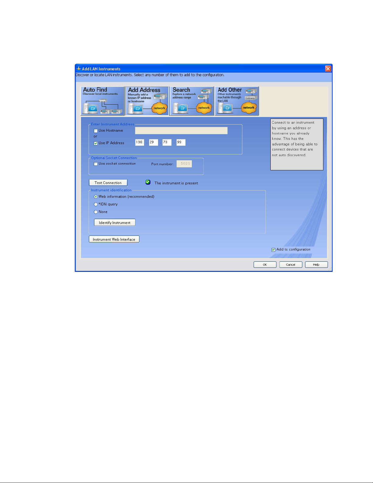
Otherwise, if the instrument is not on the same subnet, click Add
Address.

i In the next dialog, select either Hostname or IP address, and enter

the oscilloscope's hostname or IP address.

ii Click Te st Con ne cti on .

Agilent InfiniiVision 3000 X-Series Oscilloscopes Programmer's Guide 43

2 Setting Up

iii If the instrument is successfully opened, click OK to close the

dialog. If the instrument is not opened successfully, go back and
verify the LAN connections and the oscilloscope setup.

44 Agilent InfiniiVision 3000 X-Series Oscilloscopes Programmer's Guide

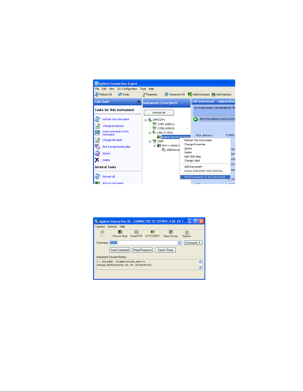
3 Test some commands on the instrument:

a Right- click on the instrument and choose Send Commands To This

Instrument from the popup menu.

Setting Up 2

b In the Agilent Interactive IO application, enter commands in the

Command field and press Send Command, Read Response, or Send&Read.

c Choose Connect>Exit from the menu to exit the Agilent Interactive IO

application.

4 In the Agilent Connection Expert application, choose File>Exit from the

menu to exit the application.

Agilent InfiniiVision 3000 X-Series Oscilloscopes Programmer's Guide 45

2 Setting Up

46 Agilent InfiniiVision 3000 X-Series Oscilloscopes Programmer's Guide

Agilent InfiniiVision 3000 X-Series Oscilloscopes

NOTE

Programmer's Guide

3
Getting Started

Basic Oscilloscope Program Structure 48
Programming the Oscilloscope 50
Other Ways of Sending Commands 59

This chapter gives you an overview of programming the 3000 X-Series
oscilloscopes. It describes basic oscilloscope program structure and shows
how to program the oscilloscope using a few simple examples.

The getting started examples show how to send oscilloscope setup, data
capture, and query commands, and they show how to read query results.

Language for Program Examples

The programming examples in this guide are written in Visual Basic using the Agilent VISA
COM library.



47

3 Getting Started

Basic Oscilloscope Program Structure

The following figure shows the basic structure of every program you will
write for the oscilloscope.

Initializing

To ensure consistent, repeatable performance, you need to start the
program, controller, and oscilloscope in a known state. Without correct
initialization, your program may run correctly in one instance and not in
another. This might be due to changes made in configuration by previous
program runs or from the front panel of the oscilloscope.

• Program initialization defines and initializes variables, allocates

memory, or tests system configuration.

• Controller initialization ensures that the interface to the oscilloscope is

properly set up and ready for data transfer.

• Oscilloscope initialization sets the channel configuration, channel labels,

threshold voltages, trigger specification, trigger mode, timebase, and
acquisition type.

Capturing Data

Once you initialize the oscilloscope, you can begin capturing data for
analysis. Remember that while the oscilloscope is responding to commands
from the controller, it is not performing acquisitions. Also, when you
change the oscilloscope configuration, any data already captured will most
likely be rendered.

To collect data, you use the :DIGitize command. This command clears the
waveform buffers and starts the acquisition process. Acquisition continues
until acquisition memory is full, then stops. The acquired data is displayed
by the oscilloscope, and the captured data can be measured, stored in

48 Agilent InfiniiVision 3000 X-Series Oscilloscopes Programmer's Guide

acquisition memory in the oscilloscope, or transferred to the controller for
further analysis. Any additional commands sent while :DIGitize is working
are buffered until :DIGitize is complete.

You could also put the oscilloscope into run mode, then use a wait loop in
your program to ensure that the oscilloscope has completed at least one
acquisition before you make a measurement. Agilent does not recommend
this because the needed length of the wait loop may vary, causing your
program to fail. :DIGitize, on the other hand, ensures that data capture is
complete. Also, :DIGitize, when complete, stops the acquisition process so
that all measurements are on displayed data, not on a constantly changing
data set.

Analyzing Captured Data

After the oscilloscope has completed an acquisition, you can find out more
about the data, either by using the oscilloscope measurements or by
transferring the data to the controller for manipulation by your program.
Built- in measurements include: frequency, duty cycle, period, positive
pulse width, and negative pulse width.

Getting Started 3

Using the :WAVeform commands, you can transfer the data to your
controller. You may want to display the data, compare it to a known good
measurement, or simply check logic patterns at various time intervals in
the acquisition.

Agilent InfiniiVision 3000 X-Series Oscilloscopes Programmer's Guide 49

3 Getting Started

Programming the Oscilloscope

• "Referencing the IO Library" on page 50

• "Opening the Oscilloscope Connection via the IO Library" on page 51

• "Using :AUToscale to Automate Oscilloscope Setup" on page 52

• "Using Other Oscilloscope Setup Commands" on page 52

• "Capturing Data with the :DIGitize Command" on page 53

• "Reading Query Responses from the Oscilloscope" on page 55

• "Reading Query Results into String Variables" on page 56

• "Reading Query Results into Numeric Variables" on page 56

• "Reading Definite- Length Block Query Response Data" on page 56

• "Sending Multiple Queries and Reading Results" on page 57

• "Checking Instrument Status" on page 58

Referencing the IO Library

No matter which instrument programming library you use (SICL, VISA, or
VISA COM), you must reference the library from your program.

In C/C++, you must tell the compiler where to find the include and library
files (see the Agilent IO Libraries Suite documentation for more
information).

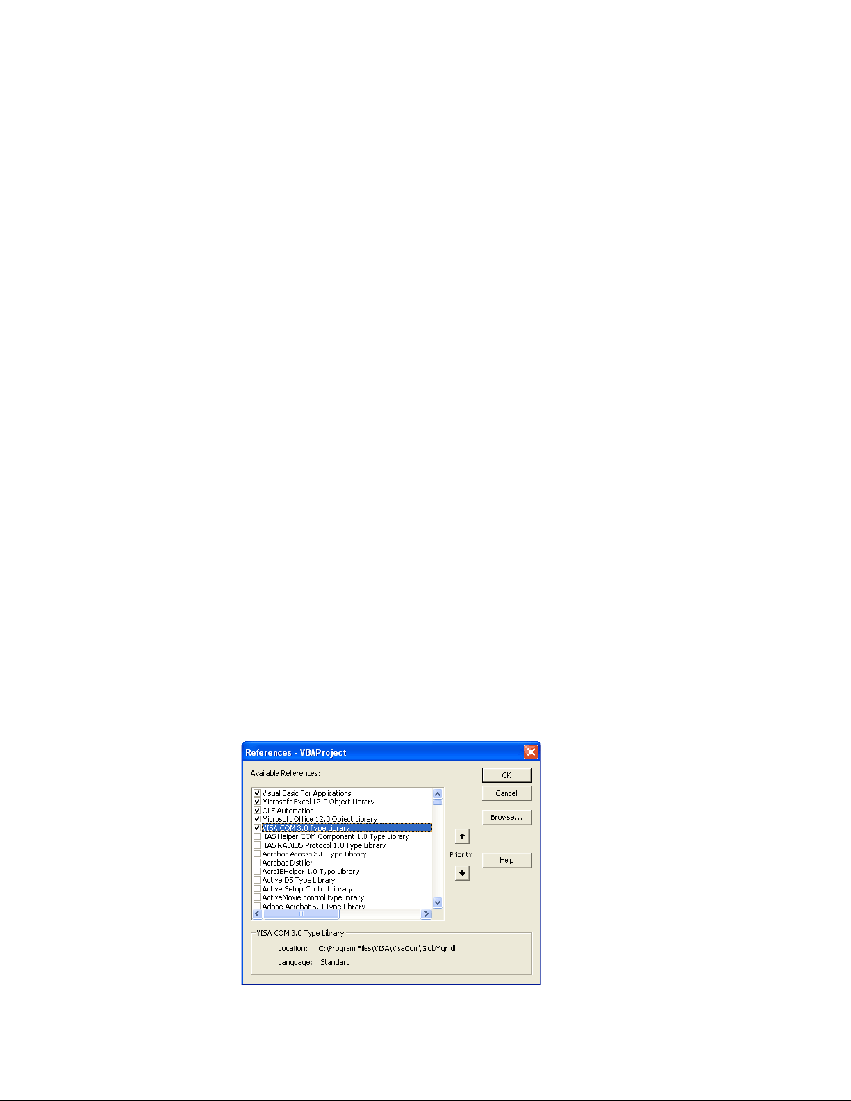
To reference the Agilent VISA COM library in Visual Basic for Applications
(VBA, which comes with Microsoft Office products like Excel):

1 Choose Tools>References... from the main menu.
2 In the References dialog, check the "VISA COM 3.0 Type Library".

50 Agilent InfiniiVision 3000 X-Series Oscilloscopes Programmer's Guide

3 Click OK.

To reference the Agilent VISA COM library in Microsoft Visual Basic 6.0:

1 Choose Project>References... from the main menu.
2 In the References dialog, check the "VISA COM 3.0 Type Library".
3 Click OK.

Opening the Oscilloscope Connection via the IO Library

PC controllers communicate with the oscilloscope by sending and receiving
messages over a remote interface. Once you have opened a connection to
the oscilloscope over the remote interface, programming instructions
normally appear as ASCII character strings embedded inside write
statements of the programing language. Read statements are used to read
query responses from the oscilloscope.

For example, when using the Agilent VISA COM library in Visual Basic
(after opening the connection to the instrument using the
ResourceManager object's Open method), the FormattedIO488 object's
WriteString, WriteNumber, WriteList, or WriteIEEEBlock methods are used
for sending commands and queries. After a query is sent, the response is
read using the ReadString, ReadNumber, ReadList, or ReadIEEEBlock
methods.

Getting Started 3

The following Visual Basic statements open the connection and send a
command that turns on the oscilloscope's label display.

Dim myMgr As VisaComLib.ResourceManager
Dim myScope As VisaComLib.FormattedIO488

Set myMgr = New VisaComLib.ResourceManager
Set myScope = New VisaComLib.FormattedIO488

' Open the connection to the oscilloscope. Get the VISA Address from the
' Agilent Connection Expert (installed with Agilent IO Libraries Suite).
Set myScope.IO = myMgr.Open("<VISA Address>")

' Send a command.
myScope.WriteString ":DISPlay:LABel ON"

The ":DISPLAY:LABEL ON" in the above example is called a program
message. Program messages are explained in more detail in "Program

Message Syntax" on page 887.

Initializing the Interface and the Oscilloscope

To make sure the bus and all appropriate interfaces are in a known state,
begin every program with an initialization statement. When using the
Agilent VISA COM library, you can use the resource session object's Clear
method to clears the interface buffer:

Agilent InfiniiVision 3000 X-Series Oscilloscopes Programmer's Guide 51

3 Getting Started

NOTE

Dim myMgr As VisaComLib.ResourceManager
Dim myScope As VisaComLib.FormattedIO488

Set myMgr = New VisaComLib.ResourceManager
Set myScope = New VisaComLib.FormattedIO488

' Open the connection to the oscilloscope. Get the VISA Address from the
' Agilent Connection Expert (installed with Agilent IO Libraries Suite).
Set myScope.IO = myMgr.Open("<VISA Address>")

' Clear the interface buffer and set the interface timeout to 10 seconds
.
myScope.IO.Clear
myScope.IO.Timeout = 10000

When you are using GPIB, CLEAR also resets the oscilloscope's parser. The
parser is the program which reads in the instructions which you send it.

After clearing the interface, initialize the instrument to a preset state:

myScope.WriteString "*RST"

Information for Initializing the Instrument

The actual commands and syntax for initializing the instrument are discussed in Chapter 5,
“Common (*) Commands,” starting on page 131.

Refer to the Agilent IO Libraries Suite documentation for information on initializing the
interface.

Using :AUToscale to Automate Oscilloscope Setup

The :AUToscale command performs a very useful function for unknown
waveforms by setting up the vertical channel, time base, and trigger level
of the instrument.

The syntax for the autoscale command is:

myScope.WriteString ":AUToscale"

Using Other Oscilloscope Setup Commands

A typical oscilloscope setup would set the vertical range and offset voltage,
the horizontal range, delay time, delay reference, trigger mode, trigger
level, and slope. An example of the commands that might be sent to the
oscilloscope are:

myScope.WriteString ":CHANnel1:PROBe 10"
myScope.WriteString ":CHANnel1:RANGe 16"
myScope.WriteString ":CHANnel1:OFFSet 1.00"
myScope.WriteString ":TIMebase:MODE MAIN"
myScope.WriteString ":TIMebase:RANGe 1E-3"
myScope.WriteString ":TIMebase:DELay 100E-6"

52 Agilent InfiniiVision 3000 X-Series Oscilloscopes Programmer's Guide

Getting Started 3

Vertical is set to 16 V full- scale (2 V/div) with center of screen at 1 V and
probe attenuation set to 10. This example sets the time base at 1 ms
full- scale (100 ms/div) with a delay of 100 µs.

Example Oscilloscope Setup Code

This program demonstrates the basic command structure used to program
the oscilloscope.

' Initialize the instrument interface to a known state.
myScope.IO.Clear
myScope.IO.Timeout = 10000 ' Set interface timeout to 10 seconds.

' Initialize the instrument to a preset state.
myScope.WriteString "*RST"

' Set the time base mode to normal with the horizontal time at
' 50 ms/div with 0 s of delay referenced at the center of the
' graticule.
myScope.WriteString ":TIMebase:RANGe 5E-4" ' Time base to 50 us/div.
myScope.WriteString ":TIMebase:DELay 0" ' Delay to zero.
myScope.WriteString ":TIMebase:REFerence CENTer" ' Display ref. at

' center.

' Set the vertical range to 1.6 volts full scale with center screen
' at -0.4 volts with 10:1 probe attenuation and DC coupling.
myScope.WriteString ":CHANnel1:PROBe 10" ' Probe attenuation

myScope.WriteString ":CHANnel1:RANGe 1.6" ' Vertical range

myScope.WriteString ":CHANnel1:OFFSet -0.4" ' Offset to -0.4.
myScope.WriteString ":CHANnel1:COUPling DC" ' Coupling to DC.

' Configure the instrument to trigger at -0.4 volts with normal
' triggering.
myScope.WriteString ":TRIGger:SWEep NORMal" ' Normal triggering.
myScope.WriteString ":TRIGger:LEVel -0.4" ' Trigger level to -0.4.
myScope.WriteString ":TRIGger:SLOPe POSitive" ' Trigger on pos. slope.

' Configure the instrument for normal acquisition.
myScope.WriteString ":ACQuire:TYPE NORMal" ' Normal acquisition.

Capturing Data with the :DIGitize Command

The :DIGitize command captures data that meets the specifications set up
by the :ACQuire subsystem. When the digitize process is complete, the
acquisition is stopped. The captured data can then be measured by the
instrument or transferred to the controller for further analysis. The
captured data consists of two parts: the waveform data record, and the
preamble.

' to 10:1.

' 1.6 V full scale.

Agilent InfiniiVision 3000 X-Series Oscilloscopes Programmer's Guide 53

3 Getting Started

NOTE

NOTE

Ensure New Data is Collected

When you change the oscilloscope configuration, the waveform buffers are cleared. Before
doing a measurement, send the :DIGitize command to the oscilloscope to ensure new data
has been collected.

When you send the :DIGitize command to the oscilloscope, the specified
channel signal is digitized with the current :ACQuire parameters. To obtain
waveform data, you must specify the :WAVeform parameters for the
SOURce channel, the FORMat type, and the number of POINts prior to
sending the :WAVeform:DATA? query.

Set :TIMebase:MODE to MAIN when using :DIGitize

:TIMebase:MODE must be set to MAIN to perform a :DIGitize command or to perform any
:WAVeform subsystem query. A "Settings conflict" error message will be returned if these
commands are executed when MODE is set to ROLL, XY, or WINDow (zoomed). Sending the
*RST (reset) command will also set the time base mode to normal.

The number of data points comprising a waveform varies according to the
number requested in the :ACQuire subsystem. The :ACQuire subsystem
determines the number of data points, type of acquisition, and number of
averages used by the :DIGitize command. This allows you to specify exactly
what the digitized information contains.

The following program example shows a typical setup:

myScope.WriteString ":ACQuire:TYPE AVERage"
myScope.WriteString ":ACQuire:COMPlete 100"
myScope.WriteString ":ACQuire:COUNt 8"
myScope.WriteString ":DIGitize CHANnel1"
myScope.WriteString ":WAVeform:SOURce CHANnel1"
myScope.WriteString ":WAVeform:FORMat BYTE"
myScope.WriteString ":WAVeform:POINts 500"
myScope.WriteString ":WAVeform:DATA?"

This setup places the instrument into the averaged mode with eight
averages. This means that when the :DIGitize command is received, the
command will execute until the signal has been averaged at least eight
times.

After receiving the :WAVeform:DATA? query, the instrument will start
passing the waveform information.

Digitized waveforms are passed from the instrument to the controller by
sending a numerical representation of each digitized point. The format of
the numerical representation is controlled with the :WAVeform:FORMat
command and may be selected as BYTE, WORD, or ASCii.

54 Agilent InfiniiVision 3000 X-Series Oscilloscopes Programmer's Guide

The easiest method of transferring a digitized waveform depends on data

NOTE

structures, formatting available and I/O capabilities. You must scale the
integers to determine the voltage value of each point. These integers are
passed starting with the left most point on the instrument's display.

For more information, see the waveform subsystem commands and
corresponding program code examples in Chapter 29, “:WAVeform
Commands,” starting on page 731.

Aborting a Digitize Operation Over the Programming Interface

When using the programming interface, you can abort a digitize operation by sending a
Device Clear over the bus (for example, myScope.IO.Clear).

Reading Query Responses from the Oscilloscope

After receiving a query (command header followed by a question mark),
the instrument interrogates the requested function and places the answer
in its output queue. The answer remains in the output queue until it is
read or another command is issued. When read, the answer is transmitted
across the interface to the designated listener (typically a controller).

Getting Started 3

The statement for reading a query response message from an instrument's
output queue typically has a format specification for handling the response
message.

When using the VISA COM library in Visual Basic, you use different read
methods (ReadString, ReadNumber, ReadList, or ReadIEEEBlock) for the
various query response formats. For example, to read the result of the
query command :CHANnel1:COUPling? you would execute the statements:

myScope.WriteString ":CHANnel1:COUPling?"
Dim strQueryResult As String
strQueryResult = myScope.ReadString

This reads the current setting for the channel one coupling into the string
variable strQueryResult.

All results for queries (sent in one program message) must be read before
another program message is sent.

Sending another command before reading the result of the query clears
the output buffer and the current response. This also causes an error to
be placed in the error queue.

Executing a read statement before sending a query causes the controller to
wait indefinitely.

The format specification for handling response messages depends on the
programming language.

Agilent InfiniiVision 3000 X-Series Oscilloscopes Programmer's Guide 55

3 Getting Started

NOTE

Reading Query Results into String Variables

The output of the instrument may be numeric or character data depending
on what is queried. Refer to the specific command descriptions for the
formats and types of data returned from queries.

Express String Variables Using Exact Syntax

In Visual Basic, string variables are case sensitive and must be expressed exactly the same
each time they are used.

The following example shows numeric data being returned to a string
variable:

myScope.WriteString ":CHANnel1:RANGe?"
Dim strQueryResult As String
strQueryResult = myScope.ReadString
MsgBox "Range (string):" + strQueryResult

After running this program, the controller displays:

Range (string): +40.0E+00

Reading Query Results into Numeric Variables

The following example shows numeric data being returned to a numeric
variable:

myScope.WriteString ":CHANnel1:RANGe?"
Dim varQueryResult As Variant
varQueryResult = myScope.ReadNumber
MsgBox "Range (variant):" + CStr(varQueryResult)

After running this program, the controller displays:

Range (variant): 40

Reading Definite-Length Block Query Response Data

Definite- length block query response data allows any type of
device-dependent data to be transmitted over the system interface as a
series of 8- bit binary data bytes. This is particularly useful for sending
large quantities of data or 8- bit extended ASCII codes. The syntax is a
pound sign (#) followed by a non-zero digit representing the number of
digits in the decimal integer. After the non-zero digit is the decimal
integer that states the number of 8-bit data bytes being sent. This is
followed by the actual data.

For example, for transmitting 1000 bytes of data, the syntax would be:

56 Agilent InfiniiVision 3000 X-Series Oscilloscopes Programmer's Guide

Getting Started 3

AXSDRNEC@S@SDQLHM@SNQ

"BST@K%@S@

/TLADQNE#XSDR
SNAD5Q@MRLHSSDC

/TLADQNE%HFHSR

5G@S'NKKNV

Figure 2 Definite-length block response data

The "8" states the number of digits that follow, and "00001000" states the
number of bytes to be transmitted.

The VISA COM library's ReadIEEEBlock and WriteIEEEBlock methods
understand the definite- length block syntax, so you can simply use
variables that contain the data:

' Read oscilloscope setup using ":SYSTem:SETup?" query.
myScope.WriteString ":SYSTem:SETup?"
Dim varQueryResult As Variant
varQueryResult = myScope.ReadIEEEBlock(BinaryType_UI1)

' Write learn string back to oscilloscope using ":SYSTem:SETup" command:
myScope.WriteIEEEBlock ":SYSTem:SETup ", varQueryResult

Sending Multiple Queries and Reading Results

You can send multiple queries to the instrument within a single command
string, but you must also read them back as a single query result. This can
be accomplished by reading them back into a single string variable,
multiple string variables, or multiple numeric variables.

For example, to read the :TIMebase:RANGe?;DELay? query result into a
single string variable, you could use the commands:

myScope.WriteString ":TIMebase:RANGe?;DELay?"
Dim strQueryResult As String
strQueryResult = myScope.ReadString
MsgBox "Timebase range; delay:" + strQueryResult

When you read the result of multiple queries into a single string variable,
each response is separated by a semicolon. For example, the output of the
previous example would be:

Timebase range; delay: <range_value>;<delay_value>

To read the :TIMebase:RANGe?;DELay? query result into multiple string
variables, you could use the ReadList method to read the query results
into a string array variable using the commands:

Agilent InfiniiVision 3000 X-Series Oscilloscopes Programmer's Guide 57

myScope.WriteString ":TIMebase:RANGe?;DELay?"
Dim strResults() As String
strResults() = myScope.ReadList(ASCIIType_BSTR)
MsgBox "Timebase range: " + strResults(0) + ", delay: " + strResults(1)

3 Getting Started

Checking Instrument Status

To read the :TIMebase:RANGe?;DELay? query result into multiple numeric
variables, you could use the ReadList method to read the query results
into a variant array variable using the commands:

myScope.WriteString ":TIMebase:RANGe?;DELay?"
Dim varResults() As Variant
varResults() = myScope.ReadList
MsgBox "Timebase range: " + FormatNumber(varResults(0) * 1000, 4) + _

" ms, delay: " + FormatNumber(varResults(1) * 1000000, 4) + " us"

Status registers track the current status of the instrument. By checking
the instrument status, you can find out whether an operation has been
completed, whether the instrument is receiving triggers, and more.

For more information, see Chapter 34, “Status Reporting,” starting on page
855 which explains how to check the status of the instrument.

58 Agilent InfiniiVision 3000 X-Series Oscilloscopes Programmer's Guide

Other Ways of Sending Commands

Standard Commands for Programmable Instrumentation (SCPI) can also be
sent via a Telnet socket or through the Browser Web Control:

• "Telnet Sockets" on page 59

• "Sending SCPI Commands Using Browser Web Control" on page 59

Telnet Sockets

The following information is provided for programmers who wish to
control the oscilloscope with SCPI commands in a Telnet session.

To connect to the oscilloscope via a telnet socket, issue the following
command:

telnet <hostname> 5024

where <hostname> is the hostname of the oscilloscope. This will give you a
command line with prompt.

Getting Started 3

For a command line without a prompt, use port 5025. For example:

telnet <hostname> 5025

Sending SCPI Commands Using Browser Web Control

To send SCPI commands using the Browser Web Control feature, establish
a connection to the oscilloscope via LAN as described in the InfiniiVision
3000 X- Series Oscilloscopes User's Guide. When you make the connection
to the oscilloscope via LAN and the instrument's welcome page is
displayed, select the Browser Web Control tab, then select the Remote

Programming link.

Agilent InfiniiVision 3000 X-Series Oscilloscopes Programmer's Guide 59

3 Getting Started

60 Agilent InfiniiVision 3000 X-Series Oscilloscopes Programmer's Guide

Agilent InfiniiVision 3000 X-Series Oscilloscopes
Programmer's Guide

4
Commands Quick Reference

Command Summary 62
Syntax Elements 127



61

4 Commands Quick Reference

Command Summary

• Common (*) Commands Summary (see page 63)

• Root (:) Commands Summary (see page 67)

• :ACQuire Commands Summary (see page 70)

• :BUS<n> Commands Summary (see page 70)

• :CALibrate Commands Summary (see page 71)

• :CHANnel<n> Commands Summary (see page 72)

• :DEMO Commands Summary (see page 74)

• :DIGital<n> Commands Summary (see page 74)

• :DISPlay Commands Summary (see page 75)

• :EXTernal Trigger Commands Summary (see page 75)

• :FUNCtion Commands Summary (see page 76)

• :HARDcopy Commands Summary (see page 78)

• :LISTer Commands Summary (see page 79)

• :MARKer Commands Summary (see page 79)

• :MEASure Commands Summary (see page 81)

• :MTESt Commands Summary (see page 90)

• :POD<n> Commands Summary (see page 92)

• :RECall Commands Summary (see page 93)

• :SAVE Commands Summary (see page 94)

• General :SBUS<n> Commands Summary (see page 95)

• :SBUS<n>:CAN Commands Summary (see page 95)

• :SBUS<n>:I2S Commands Summary (see page 97)

• :SBUS<n>:IIC Commands Summary (see page 99)

• :SBUS<n>:LIN Commands Summary (see page 100)

• :SBUS<n>:SPI Commands Summary (see page 101

• :SBUS<n>:UART Commands Summary (see page 103)

• General :SEARch Commands Summary (see page 105)

• :SEARch:EDGE Commands Summary (see page 106)

• :SEARch:GLITch Commands Summary (see page 106)

)

• :SEARch:RUNT Commands Summary (see page 107)

• :SEARch:TRANsition Commands Summary (see page 107)

• :SEARch:SERial:CAN Commands Summary (see page 107)

• :SEARch:SERial:I2S Commands Summary (see page 108)

62 Agilent InfiniiVision 3000 X-Series Oscilloscopes Programmer's Guide

Commands Quick Reference 4

• :SEARch:SERial:IIC Commands Summary (see page 109)

• :SEARch:SERial:LIN Commands Summary (see page 110)

• :SEARch:SERial:SPI Commands Summary (see page 110)

• :SEARch:SERial:UART Commands Summary (see page 111)

• :SYSTem Commands Summary (see page 111)

• :TIMebase Commands Summary (see page 112)

• General :TRIGger Commands Summary (see page 113)

• :TRIGger:DELay Commands Summary (see page 114)

• :TRIGger:EBURst Commands Summary (see page 114)

• :TRIGger[:EDGE] Commands Summary (see page 115)

• :TRIGger:GLITch Commands Summary (see page 116)

• :TRIGger:OR Commands Summary (see page 117)

• :TRIGger:PATTern Commands Summary (see page 118)

• :TRIGger:RUNT Commands Summary (see page 119)

• :TRIGger:SHOLd Commands Summary (see page 119)

• :TRIGger:TRANsition Commands Summary (see page 120)

• :TRIGger:TV Commands Summary (see page 120)

• :TRIGger:USB Commands Summary (see page 121)

• :WAVeform Commands Summary (see page 121)

• :WGEN Commands Summary (see page 124)

• :WMEMory<r> Commands Summary (see page 125)

Table 2 Common (*) Commands Summary

Command Query Options and Query Returns

*CLS (see page 135) n/a n/a

*ESE <mask> (see

page 136)

*ESE? (see page 136) <mask> ::= 0 to 255; an integer

in NR1 format:

Bit Weight Name Enables

--- ------ ---- ---------­7 128 PON Power On
6 64 URQ User Request
5 32 CME Command Error
4 16 EXE Execution Error
3 8 DDE Dev. Dependent Error
2 4 QYE Query Error
1 2 RQL Request Control
0 1 OPC Operation Complete

n/a *ESR? (see page 138) <status> ::= 0 to 255; an integer

in NR1 format

Agilent InfiniiVision 3000 X-Series Oscilloscopes Programmer's Guide 63

4 Commands Quick Reference

Table 2 Common (*) Commands Summary (continued)

Command Query Options and Query Returns

n/a *IDN? (see page 138) AGILENT

TECHNOLOGIES,<model>,<serial
number>,X.XX.XX
<model> ::= the model number of
the instrument

<serial number> ::= the serial
number of the instrument

<X.XX.XX> ::= the software
revision of the instrument

n/a *LRN? (see page 141) <learn_string> ::= current

instrument setup as a block of
data in IEEE 488.2 # format

*OPC (see page 142) *OPC? (see page 142) ASCII "1" is placed in the output

queue when all pending device
operations have completed.

64 Agilent InfiniiVision 3000 X-Series Oscilloscopes Programmer's Guide

Commands Quick Reference 4

Table 2 Common (*) Commands Summary (continued)

Command Query Options and Query Returns

n/a *OPT? (see page 143) <return_value> ::= 0,0,<license

info>
<license info> ::= <All field>,
<reserved>, <MSO>, <reserved>,
<Memory>, <Low Speed Serial>,
<Automotive Serial>, <reserved>,
<reserved>,
<Power Measurements>,
<RS-232/UART Serial>,
<Segmented Memory>, <Mask Test>,
<reserved>, <Bandwidth>,
<reserved>, <reserved>,
<reserved>, <I2S Serial>,
<reserved>, <reserved>,
<Waveform Generator>,
<reserved>, <reserved>
<All field> ::= {0 | All}
<reserved> ::= 0
<MSO> ::= {0 | MSO}
<Memory> ::= {0 | MEMUP}
<Low Speed Serial> ::= {0 | EMBD}
<Automotive Serial> ::= {0 |
AUTO}
<Power Measurements> ::= {0 |
PWR}
<RS-232/UART Serial> ::= {0 |
COMP}
<Segmented Memory> ::= {0 | SGM}
<Mask Test> ::= {0 | MASK}
<Bandwidth> ::= {0 | BW20 | BW50}
<I2S Serial> ::= {0 | AUDIO}
<Waveform Generator> ::= {0 |
WAVEGEN}

*RCL <value> (see

page 145)

*RST (see page 146) n/a See *RST (Reset) (see page 146)

*SAV <value> (see

page 149)

Agilent InfiniiVision 3000 X-Series Oscilloscopes Programmer's Guide 65

n/a <value> ::= {0 | 1 | 4 | 5 | 6 |

7 | 8 | 9}

n/a <value> ::= {0 | 1 | 4 | 5 | 6 |

7 | 8 | 9}

4 Commands Quick Reference

Table 2 Common (*) Commands Summary (continued)

Command Query Options and Query Returns

*SRE <mask> (see

page 150)

*SRE? (see page 151) <mask> ::= sum of all bits that

are set, 0 to 255; an integer in
NR1 format. <mask> ::= following
values:

Bit Weight Name Enables

--- ------ ---- ---------­7 128 OPER Operation Status Reg
6 64 ---- (Not used.)
5 32 ESB Event Status Bit
4 16 MAV Message Available
3 8 ---- (Not used.)
2 4 MSG Message
1 2 USR User
0 1 TRG Trigger

n/a *STB? (see page 152) <value> ::= 0 to 255; an integer

in NR1 format, as shown in the
following:

Bit Weight Name "1" Indicates

--- ------ ---- --------------­7 128 OPER Operation status

condition occurred.

6 64 RQS/ Instrument is

5 32 ESB Enabled event status

4 16 MAV Message available.
3 8 ---- (Not used.)
2 4 MSG Message displayed.
1 2 USR User event

0 1 TRG A trigger occurred.

MSS requesting service.

condition occurred.

condition occurred.

*TRG (see page 154) n/a n/a

n/a *TST? (see page 155) <result> ::= 0 or non-zero value;

an integer in NR1 format

*WAI (see page 156) n/a n/a

66 Agilent InfiniiVision 3000 X-Series Oscilloscopes Programmer's Guide

Commands Quick Reference 4

Table 3 Root (:) Commands Summary

Command Query Options and Query Returns

:ACTivity (see

page 161)

n/a :AER? (see page 162) {0 | 1}; an integer in NR1 format

:AUToscale
[<source>[,..,<source
>]] (see page 163)

:AUToscale:AMODE
<value> (see

page 165)

:ACTivity? (see

page 161)

n/a <source> ::= CHANnel<n> for DSO

:AUToscale:AMODE?
(see page 165)

<return value> ::=
<edges>,<levels>
<edges> ::= presence of edges
(32-bit integer in NR1 format)

<levels> ::= logical highs or
lows (32-bit integer in NR1
format)

models
<source> ::= {CHANnel<n> |

DIGital<d> | POD1 | POD2} for MSO
models

<source> can be repeated up to 5
times
<n> ::= 1 to (# analog channels)
in NR1 format

<d> ::= 0 to (# digital channels

- 1) in NR1 format

<value> ::= {NORMal | CURRent}}

:AUToscale:CHANnels
<value> (see

page 166)

:AUToscale:FDEBug {{0
| OFF} | {1 | ON}}
(see page 167)

:BLANk [<source>]
(see page 168)

:AUToscale:CHANnels?
(see page 166)

:AUToscale:FDEBug?
(see page 167)

n/a <source> ::= {CHANnel<n>} |

<value> ::= {ALL | DISPlayed}}

{0 | 1}

FUNCtion | MATH | SBUS{1 | 2}}
for DSO models

<source> ::= {CHANnel<n> |
DIGital<d> | POD{1 | 2} | BUS{1 |
2} | FUNCtion | MATH | SBUS{1 |
2}} for MSO models
<n> ::= 1 to (# analog channels)
in NR1 format

<d> ::= 0 to (# digital channels

- 1) in NR1 format

Agilent InfiniiVision 3000 X-Series Oscilloscopes Programmer's Guide 67

4 Commands Quick Reference

Table 3 Root (:) Commands Summary (continued)

Command Query Options and Query Returns

:DIGitize
[<source>[,..,<source
>]] (see page 169)

:MTEenable <n> (see

page 171)

n/a :MTERegister[:EVENt]?

:OPEE <n> (see

page 175)

n/a :OPERregister:CONDiti

n/a <source> ::= {CHANnel<n> |

:MTEenable? (see

page 171)

(see page 173)

:OPEE? (see page 175) <n> ::= 15-bit integer in NR1

on? (see page 177)

FUNCtion | MATH | SBUS{1 | 2}}
for DSO models
<source> ::= {CHANnel<n> |
DIGital<d> | POD{1 | 2} | BUS{1 |
2} | FUNCtion | MATH | SBUS{1 |
2}} for MSO models

<source> can be repeated up to 5
times

<n> ::= 1 to (# analog channels)
in NR1 format
<d> ::= 0 to (# digital channels

- 1) in NR1 format

<n> ::= 16-bit integer in NR1
format

<n> ::= 16-bit integer in NR1
format

format

<n> ::= 15-bit integer in NR1
format

n/a :OPERegister[:EVENt]?

(see page 179)

:OVLenable <mask>
(see page 181)

n/a :OVLRegister? (see

:OVLenable? (see

page 182)

page 183)

<n> ::= 15-bit integer in NR1
format

<mask> ::= 16-bit integer in NR1
format as shown:

Bit Weight Input

--- ------ ----------

10 1024 Ext Trigger Fault

9 512 Channel 4 Fault
8 256 Channel 3 Fault
7 128 Channel 2 Fault
6 64 Channel 1 Fault
4 16 Ext Trigger OVL
3 8 Channel 4 OVL
2 4 Channel 3 OVL
1 2 Channel 2 OVL
0 1 Channel 1 OVL

<value> ::= integer in NR1
format. See OVLenable for <value>

68 Agilent InfiniiVision 3000 X-Series Oscilloscopes Programmer's Guide

Commands Quick Reference 4

Table 3 Root (:) Commands Summary (continued)

Command Query Options and Query Returns

:PRINt [<options>]
(see page 185)

:RUN (see page 186) n/a n/a

n/a :SERial (see

:SINGle (see

page 188)

n/a :STATus? <display>

n/a <options> ::= [<print

option>][,..,<print option>]
<print option> ::= {COLor |
GRAYscale | PRINter0 | BMP8bit |
BMP | PNG | NOFactors | FACTors}
<print option> can be repeated up
to 5 times.

<return value> ::= unquoted

page 187)

n/a n/a

(see page 189)

string containing serial number

{0 | 1}
<display> ::= {CHANnel<n> |
DIGital<d> | POD{1 | 2} | BUS{1 |
2} | FUNCtion | MATH | SBUS{1 |
2}}
<n> ::= 1 to (# analog channels)
in NR1 format
<d> ::= 0 to (# digital channels

- 1) in NR1 format

:STOP (see page 190) n/a n/a

n/a :TER? (see page 191) {0 | 1}

:VIEW <source> (see

page 192)

n/a <source> ::= {CHANnel<n> |

FUNCtion | MATH | SBUS{1 | 2}}
for DSO models

<source> ::= {CHANnel<n> |
DIGital<d> | POD{1 | 2} | BUS{1 |
2} | FUNCtion | MATH | SBUS{1 |
2}} for MSO models
<n> ::= 1 to (# analog channels)
in NR1 format

<d> ::= 0 to (# digital channels

- 1) in NR1 format

Agilent InfiniiVision 3000 X-Series Oscilloscopes Programmer's Guide 69

4 Commands Quick Reference

Table 4 :ACQuire Commands Summary

Command Query Options and Query Returns

:ACQuire:COMPlete
<complete> (see

page 195)

:ACQuire:COUNt
<count> (see

page 196)

:ACQuire:MODE <mode>
(see page 197)

n/a :ACQuire:POINts? (see

:ACQuire:SEGMented:AN
ALyze (see page 199)

:ACQuire:SEGMented:CO
UNt <count> (see

page 200)

:ACQuire:SEGMented:IN
Dex <index> (see

page 201)

n/a :ACQuire:SRATe? (see

:ACQuire:COMPlete?
(see page 195)

:ACQuire:COUNt? (see

page 196)

:ACQuire:MODE? (see

page 197)

page 198)

n/a n/a (with Option SGM)

:ACQuire:SEGMented:CO
UNt? (see page 200)

:ACQuire:SEGMented:IN
Dex? (see page 201)

page 204)

<complete> ::= 100; an integer in
NR1 format

<count> ::= an integer from 2 to
65536 in NR1 format

<mode> ::= {RTIMe | SEGMented}

<# points> ::= an integer in NR1
format

<count> ::= an integer from 2 to
1000 in NR1 format (with Option
SGM)

<index> ::= an integer from 1 to
1000 in NR1 format (with Option
SGM)

<sample_rate> ::= sample rate
(samples/s) in NR3 format

:ACQuire:TYPE <type>
(see page 205)

:ACQuire:TYPE? (see

page 205)

<type> ::= {NORMal | AVERage |
HRESolution | PEAK}

Table 5 :BUS<n> Commands Summary

Command Query Options and Query Returns

:BUS<n>:BIT<m> {{0 |
OFF} | {1 | ON}} (see

page 209)

:BUS<n>:BITS
<channel_list>, {{0 |
OFF} | {1 | ON}} (see

page 210)

:BUS<n>:BIT<m>? (see

page 209)

:BUS<n>:BITS? (see

page 210)

{0 | 1}
<n> ::= 1 or 2; an integer in NR1
format
<m> ::= 0-15; an integer in NR1
format

<channel_list>, {0 | 1}
<channel_list> ::= (@<m>,<m>:<m>
...) where "," is separator and
":" is range
<n> ::= 1 or 2; an integer in NR1
format
<m> ::= 0-15; an integer in NR1
format

70 Agilent InfiniiVision 3000 X-Series Oscilloscopes Programmer's Guide

Commands Quick Reference 4

Table 5 :BUS<n> Commands Summary (continued)

Command Query Options and Query Returns

:BUS<n>:CLEar (see

page 212)

:BUS<n>:DISPlay {{0 |
OFF} | {1 | ON}} (see

page 213)

:BUS<n>:LABel
<string> (see

page 214)

:BUS<n>:MASK <mask>
(see page 215)

n/a <n> ::= 1 or 2; an integer in NR1

format

:BUS<n>:DISPlay? (see

page 213)

:BUS<n>:LABel? (see

page 214)

:BUS<n>:MASK? (see

page 215)

{0 | 1}
<n> ::= 1 or 2; an integer in NR1

format

<string> ::= quoted ASCII string
up to 10 characters
<n> ::= 1 or 2; an integer in NR1
format

<mask> ::= 32-bit integer in
decimal, <nondecimal>, or
<string>

<nondecimal> ::= #Hnn...n where n
::= {0,..,9 | A,..,F} for
hexadecimal
<nondecimal> ::= #Bnn...n where n
::= {0 | 1} for binary

<string> ::= "0xnn...n" where n
::= {0,..,9 | A,..,F} for
hexadecimal

<n> ::= 1 or 2; an integer in NR1
format

Table 6 :CALibrate Commands Summary

Command Query Options and Query Returns

n/a :CALibrate:DATE? (see

page 219)

:CALibrate:LABel
<string> (see

page 220)

:CALibrate:OUTPut
<signal> (see

page 221)

n/a :CALibrate:PROTected?

:CALibrate:STARt (see

page 223)

:CALibrate:LABel?
(see page 220)

:CALibrate:OUTPut?
(see page 221)

(see page 222)

n/a n/a

<return value> ::=
<year>,<month>,<day>; all in NR1
format

<string> ::= quoted ASCII string
up to 32 characters

<signal> ::= {TRIGgers | MASK |
WAVEgen}

{PROTected | UNPRotected}

Agilent InfiniiVision 3000 X-Series Oscilloscopes Programmer's Guide 71

4 Commands Quick Reference

Table 6 :CALibrate Commands Summary (continued)

Command Query Options and Query Returns

n/a :CALibrate:STATus?

(see page 224)

n/a :CALibrate:TEMPeratur

e? (see page 225)

n/a :CALibrate:TIME? (see

page 226)

<return value> ::=
<status_code>,<status_string>
<status_code> ::= an integer
status code

<status_string> ::= an ASCII
status string

<return value> ::= degrees C
delta since last cal in NR3
format

<return value> ::=
<hours>,<minutes>,<seconds>; all
in NR1 format

Table 7 :CHANnel<n> Commands Summary

Command Query Options and Query Returns

:CHANnel<n>:BWLimit
{{0 | OFF} | {1 |
ON}} (see page 230)

:CHANnel<n>:COUPling
<coupling> (see

page 231)

:CHANnel<n>:BWLimit?
(see page 230)

:CHANnel<n>:COUPling?
(see page 231)

{0 | 1}
<n> ::= 1 to (# analog channels)
in NR1 format

<coupling> ::= {AC | DC}
<n> ::= 1 to (# analog channels)

in NR1 format

:CHANnel<n>:DISPlay
{{0 | OFF} | {1 |
ON}} (see page 232)

:CHANnel<n>:IMPedance
<impedance> (see

page 233)

:CHANnel<n>:INVert
{{0 | OFF} | {1 |
ON}} (see page 234)

:CHANnel<n>:LABel
<string> (see

page 235)

:CHANnel<n>:OFFSet
<offset>[suffix] (see

page 236)

:CHANnel<n>:DISPlay?
(see page 232)

:CHANnel<n>:IMPedance
? (see page 233)

:CHANnel<n>:INVert?
(see page 234)

:CHANnel<n>:LABel?
(see page 235)

:CHANnel<n>:OFFSet?
(see page 236)

{0 | 1}
<n> ::= 1 to (# analog channels)

in NR1 format

<impedance> ::= {ONEMeg | FIFTy}
<n> ::= 1 to (# analog channels)

in NR1 format

{0 | 1}
<n> ::= 1 to (# analog channels)

in NR1 format

<string> ::= any series of 10 or
less ASCII characters enclosed in
quotation marks
<n> ::= 1 to (# analog channels)
in NR1 format

<offset> ::= Vertical offset
value in NR3 format

[suffix] ::= {V | mV}
<n> ::= 1-2 or 1-4; in NR1 format

72 Agilent InfiniiVision 3000 X-Series Oscilloscopes Programmer's Guide

Commands Quick Reference 4

Table 7 :CHANnel<n> Commands Summary (continued)

Command Query Options and Query Returns

:CHANnel<n>:PROBe
<attenuation> (see

page 237)

:CHANnel<n>:PROBe:HEA
D[:TYPE] <head_param>
(see page 238)

n/a :CHANnel<n>:PROBe:ID?

:CHANnel<n>:PROBe:SKE
W <skew_value> (see

page 240)

:CHANnel<n>:PROBe:STY
Pe <signal type> (see

page 241)

:CHANnel<n>:PROTectio
n (see page 242)

:CHANnel<n>:PROBe?
(see page 237)

:CHANnel<n>:PROBe:HEA
D[:TYPE]? (see

page 238)

(see page 239)

:CHANnel<n>:PROBe:SKE
W? (see page 240)

:CHANnel<n>:PROBe:STY
Pe? (see page 241)

:CHANnel<n>:PROTectio
n? (see page 242)

<attenuation> ::= Probe
attenuation ratio in NR3 format
<n> ::= 1-2 or 1-4r in NR1 format

<head_param> ::= {SEND0 | SEND6 |
SEND12 | SEND20 | DIFF0 | DIFF6 |
DIFF12 | DIFF20 | NONE}

<n> ::= 1 to (# analog channels)
in NR1 format

<probe id> ::= unquoted ASCII
string up to 11 characters

<n> ::= 1 to (# analog channels)
in NR1 format

<skew_value> ::= -100 ns to +100
ns in NR3 format
<n> ::= 1 to (# analog channels)
in NR1 format

<signal type> ::= {DIFFerential |
SINGle}

<n> ::= 1 to (# analog channels)
in NR1 format

{NORM | TRIP}
<n> ::= 1 to (# analog channels)

in NR1 format

:CHANnel<n>:RANGe
<range>[suffix] (see

page 243)

:CHANnel<n>:SCALe
<scale>[suffix] (see

page 244)

:CHANnel<n>:UNITs
<units> (see

page 245)

:CHANnel<n>:VERNier
{{0 | OFF} | {1 |
ON}} (see page 246

Agilent InfiniiVision 3000 X-Series Oscilloscopes Programmer's Guide 73

:CHANnel<n>:RANGe?
(see page 243)

:CHANnel<n>:SCALe?
(see page 244)

:CHANnel<n>:UNITs?
(see page 245)

:CHANnel<n>:VERNier?
(see page 246)

)

<range> ::= Vertical full-scale
range value in NR3 format

[suffix] ::= {V | mV}
<n> ::= 1 to (# analog channels)
in NR1 format

<scale> ::= Vertical units per
division value in NR3 format

[suffix] ::= {V | mV}
<n> ::= 1 to (# analog channels)
in NR1 format

<units> ::= {VOLT | AMPere}
<n> ::= 1 to (# analog channels)

in NR1 format

{0 | 1}
<n> ::= 1 to (# analog channels)

in NR1 format

4 Commands Quick Reference

Table 8 :DEMO Commands Summary

Command Query Options and Query Returns

:DEMO:FUNCtion
<signal> (see

page 248)

:DEMO:FUNCtion:PHASe:
PHASe <angle> (see

page 251)

:DEMO:OUTPut {{0 |
OFF} | {1 | ON}} (see

page 252)

:DEMO:FUNCtion? (see

page 250)

:DEMO:FUNCtion:PHASe:
PHASe? (see page 251)

:DEMO:OUTPut? (see

page 252)

<signal> ::= {SINusoid | NOISy |
PHASe | RINGing | SINGle | AM |
CLK | GLITch | BURSt | MSO | RUNT
| TRANsition | RFBurst | SHOLd |
LFSine | ETE | CAN | LIN | UART |
I2C | SPI | I2S | CANLin}

<angle> ::= angle in degrees from
0 to 360 in NR3 format

{0 | 1}

Table 9 :DIGital<d> Commands Summary

Command Query Options and Query Returns

:DIGital<d>:DISPlay
{{0 | OFF} | {1 |
ON}} (see page 255)

:DIGital<d>:LABel
<string> (see

page 256)

:DIGital<d>:DISPlay?
(see page 255)

:DIGital<d>:LABel?
(see page 256)

<d> ::= 0 to (# digital channels

- 1) in NR1 format

{0 | 1}

<d> ::= 0 to (# digital channels

- 1) in NR1 format

<string> ::= any series of 10 or
less ASCII characters enclosed in
quotation marks

:DIGital<d>:POSition
<position> (see

page 257)

:DIGital<d>:SIZE
<value> (see

page 258)

:DIGital<d>:THReshold
<value>[suffix] (see

page 259)

74 Agilent InfiniiVision 3000 X-Series Oscilloscopes Programmer's Guide

:DIGital<d>:POSition?
(see page 257)

:DIGital<d>:SIZE?
(see page 258)

:DIGital<d>:THReshold
? (see page 259)

<d> ::= 0 to (# digital channels

- 1) in NR1 format

<position> ::= 0-7 if display
size = large, 0-15 if size =
medium, 0-31 if size = small

Returns -1 when there is no space
to display the digital waveform.

<d> ::= 0 to (# digital channels

- 1) in NR1 format

<value> ::= {SMALl | MEDium |
LARGe}

<d> ::= 0 to (# digital channels

- 1) in NR1 format

<value> ::= {CMOS | ECL | TTL |
<user defined value>}

<user defined value> ::= value in
NR3 format from -8.00 to +8.00

[suffix] ::= {V | mV | uV}

Commands Quick Reference 4

Table 10 :DISPlay Commands Summary

Command Query Options and Query Returns

:DISPlay:CLEar (see

page 263)

n/a :DISPlay:DATA?

:DISPlay:LABel {{0 |
OFF} | {1 | ON}} (see

page 265)

:DISPlay:LABList
<binary block> (see

page 266)

:DISPlay:PERSistence
<value> (see

page 267)

:DISPlay:VECTors {1 |
ON} (see page 268)

n/a n/a

[<format>][,][<palett
e>] (see page 264)

:DISPlay:LABel? (see

page 265)

:DISPlay:LABList?
(see page 266)

:DISPlay:PERSistence?
(see page 267)

:DISPlay:VECTors?
(see page 268)

<format> ::= {BMP | BMP8bit |
PNG}

<palette> ::= {COLor | GRAYscale}
<display data> ::= data in IEEE

488.2 # format

{0 | 1}

<binary block> ::= an ordered
list of up to 75 labels, each 10
characters maximum, separated by
newline characters

<value> ::= {MINimum | INFinite |
<time>}
<time> ::= seconds in in NR3
format from 100E-3 to 60E0

1

Table 11 :EXTernal Trigger Commands Summary

Command Query Options and Query Returns

:EXTernal:BWLimit
<bwlimit> (see

page 270)

:EXTernal:PROBe
<attenuation> (see

page 271)

:EXTernal:RANGe
<range>[<suffix>]
(see page 272)

:EXTernal:UNITs
<units> (see

page 273)

:EXTernal:BWLimit?
(see page 270)

:EXTernal:PROBe? (see

page 271)

:EXTernal:RANGe? (see

page 272)

:EXTernal:UNITs? (see

page 273)

<bwlimit> ::= {0 | OFF}

<attenuation> ::= probe
attenuation ratio in NR3 format

<range> ::= vertical full-scale
range value in NR3 format

<suffix> ::= {V | mV}

<units> ::= {VOLT | AMPere}

Agilent InfiniiVision 3000 X-Series Oscilloscopes Programmer's Guide 75

4 Commands Quick Reference

Table 12 :FUNCtion Commands Summary

Command Query Options and Query Returns

:FUNCtion:DISPlay {{0
| OFF} | {1 | ON}}
(see page 278)

:FUNCtion[:FFT]:CENTe
r <frequency> (see

page 279)

:FUNCtion[:FFT]:SPAN
<span> (see page 280)

:FUNCtion[:FFT]:VTYPe
<units> (see

page 281)

:FUNCtion[:FFT]:WINDo
w <window> (see

page 282)

:FUNCtion:GOFT:OPERat
ion <operation> (see

page 283)

:FUNCtion:GOFT:SOURce
1 <source> (see

page 284)

:FUNCtion:DISPlay?
(see page 278)

:FUNCtion[:FFT]:CENTe
r? (see page 279)

:FUNCtion[:FFT]:SPAN?
(see page 280)

:FUNCtion[:FFT]:VTYPe
? (see page 281)

:FUNCtion[:FFT]:WINDo
w? (see page 282)

:FUNCtion:GOFT:OPERat
ion? (see page 283)

:FUNCtion:GOFT:SOURce
1? (see page 284)

{0 | 1}

<frequency> ::= the current
center frequency in NR3 format.
The range of legal values is from
0 Hz to 25 GHz.

<span> ::= the current frequency
span in NR3 format.

Legal values are 1 Hz to 100 GHz.

<units> ::= {DECibel | VRMS}

<window> ::= {RECTangular |
HANNing | FLATtop | BHARris}

<operation> ::= {ADD | SUBTract |
MULTiply}

<source> ::= CHANnel<n>
<n> ::= {1 | 2 | 3 | 4} for 4ch

models
<n> ::= {1 | 2} for 2ch models

:FUNCtion:GOFT:SOURce
2 <source> (see

page 285)

:FUNCtion:INTegrate:I
OFFset <input_offset>
(see page 286)

:FUNCtion:OFFSet
<offset> (see

page 287)

:FUNCtion:OPERation
<operation> (see

page 288)

76 Agilent InfiniiVision 3000 X-Series Oscilloscopes Programmer's Guide

:FUNCtion:GOFT:SOURce
2? (see page 285)

:FUNCtion:INTegrate:I
OFFset? (see

page 286)

:FUNCtion:OFFSet?
(see page 287)

:FUNCtion:OPERation?
(see page 288)

<source> ::= CHANnel<n>
<n> ::= {1 | 2 | 3 | 4} for 4ch
models
<n> ::= {1 | 2} for 2ch models

<input_offset> ::= DC offset
correction in NR3 format.

<offset> ::= the value at center
screen in NR3 format.

The range of legal values is
+/-10 times the current
sensitivity of the selected
function.

<operation> ::= {ADD | SUBTract |
MULTiply | INTegrate | DIFF | FFT
| SQRT}

Commands Quick Reference 4

Table 12 :FUNCtion Commands Summary (continued)

Command Query Options and Query Returns

:FUNCtion:RANGe
<range> (see

page 289)

:FUNCtion:REFerence
<level> (see

page 290)

:FUNCtion:SCALe
<scale
value>[<suffix>] (see

page 291)

:FUNCtion:SOURce1
<source> (see

page 292)

:FUNCtion:RANGe? (see

page 289)

:FUNCtion:REFerence?
(see page 290)

:FUNCtion:SCALe? (see

page 291)

:FUNCtion:SOURce1?
(see page 292)

<range> ::= the full-scale
vertical axis value in NR3
format.
The range for ADD, SUBT, MULT is
8E-6 to 800E+3. The range for the
INTegrate function is 8E-9 to
400E+3.

The range for the DIFF function
is 80E-3 to 8.0E12 (depends on
current sweep speed).

The range for the FFT function is
8 to 800 dBV.

<level> ::= the value at center
screen in NR3 format.

The range of legal values is
+/-10 times the current
sensitivity of the selected
function.

<scale value> ::= integer in NR1
format
<suffix> ::= {V | dB}

<source> ::= {CHANnel<n> | GOFT}
<n> ::= {1 | 2 | 3 | 4} for 4ch

models
<n> ::= {1 | 2} for 2ch models
GOFT is only for FFT, INTegrate,

DIFF, and SQRT operations.

:FUNCtion:SOURce2
<source> (see

page 293)

Agilent InfiniiVision 3000 X-Series Oscilloscopes Programmer's Guide 77

:FUNCtion:SOURce2?
(see page 293)

<source> ::= {CHANnel<n> | NONE}
<n> ::= {{1 | 2} | {3 | 4}} for

4ch models, depending on SOURce1
selection

<n> ::= {1 | 2} for 2ch models

4 Commands Quick Reference

Table 13 :HARDcopy Commands Summary

Command Query Options and Query Returns

:HARDcopy:AREA <area>
(see page 297)

:HARDcopy:APRinter
<active_printer> (see

page 298)

:HARDcopy:FACTors {{0
| OFF} | {1 | ON}}
(see page 299)

:HARDcopy:FFEed {{0 |
OFF} | {1 | ON}} (see

page 300)

:HARDcopy:INKSaver
{{0 | OFF} | {1 |
ON}} (see page 301)

:HARDcopy:LAYout
<layout> (see

page 302)

:HARDcopy:NETWork:ADD
Ress <address> (see

page 303)

:HARDcopy:AREA? (see

page 297)

:HARDcopy:APRinter?
(see page 298)

:HARDcopy:FACTors?
(see page 299)

:HARDcopy:FFEed? (see

page 300)

:HARDcopy:INKSaver?
(see page 301)

:HARDcopy:LAYout?
(see page 302)

:HARDcopy:NETWork:ADD
Ress? (see page 303)

<area> ::= SCReen

<active_printer> ::= {<index> |
<name>}

<index> ::= integer index of
printer in list

<name> ::= name of printer in
list

{0 | 1}

{0 | 1}

{0 | 1}

<layout> ::= {LANDscape |
PORTrait}

<address> ::= quoted ASCII string

:HARDcopy:NETWork:APP
Ly (see page 304)

:HARDcopy:NETWork:DOM
ain <domain> (see

page 305)

:HARDcopy:NETWork:PAS
Sword <password> (see

page 306)

:HARDcopy:NETWork:SLO
T <slot> (see

page 307)

:HARDcopy:NETWork:USE
Rname <username> (see

page 308)

:HARDcopy:PALette
<palette> (see

page 309)

78 Agilent InfiniiVision 3000 X-Series Oscilloscopes Programmer's Guide

n/a n/a

:HARDcopy:NETWork:DOM
ain? (see page 305)

n/a <password> ::= quoted ASCII

:HARDcopy:NETWork:SLO
T? (see page 307)

:HARDcopy:NETWork:USE
Rname? (see page 308

:HARDcopy:PALette?
(see page 309)

<domain> ::= quoted ASCII string

string

<slot> ::= {NET0 | NET1}

<username> ::= quoted ASCII

)

string

<palette> ::= {COLor | GRAYscale
| NONE}

Commands Quick Reference 4

Table 13 :HARDcopy Commands Summary (continued)

Command Query Options and Query Returns

n/a :HARDcopy:PRINter:LIS

T? (see page 310)

:HARDcopy:STARt (see

page 311)

n/a n/a

<list> ::= [<printer_spec>] ...
[printer_spec>]
<printer_spec> ::=
"<index>,<active>,<name>;"

<index> ::= integer index of
printer

<active> ::= {Y | N}
<name> ::= name of printer

Table 14 :LISTer Commands Summary

Command Query Options and Query Returns

n/a :LISTer:DATA? (see

page 314)

:LISTer:DISPlay {{OFF
| 0} | {SBUS1 | ON |
1} | {SBUS2 | 2} |
ALL} (see page 315)

:LISTer:DISPlay? (see

page 315)

<binary_block> ::=
comma-separated data with
newlines at the end of each row

{OFF | SBUS1 | SBUS2 | ALL}

:LISTer:REFerence
<time_ref> (see

page 316)

:LISTer:REFerence?
(see page 316)

<time_ref> ::= {TRIGger |
PREVious}

Table 15 :MARKer Commands Summary

Command Query Options and Query Returns

:MARKer:MODE <mode>
(see page 319)

:MARKer:X1Position
<position>[suffix]
(see page 320)

:MARKer:MODE? (see

page 319)

:MARKer:X1Position?
(see page 320)

<mode> ::= {OFF | MEASurement |
MANual | WAVeform}

<position> ::= X1 cursor position
value in NR3 format

[suffix] ::= {s | ms | us | ns |
ps | Hz | kHz | MHz}
<return_value> ::= X1 cursor
position value in NR3 format

Agilent InfiniiVision 3000 X-Series Oscilloscopes Programmer's Guide 79

4 Commands Quick Reference

Table 15 :MARKer Commands Summary (continued)

Command Query Options and Query Returns

:MARKer:X1Y1source
<source> (see

page 321)

:MARKer:X2Position
<position>[suffix]
(see page 322)

:MARKer:X2Y2source
<source> (see

page 323)

n/a :MARKer:XDELta? (see

:MARKer:XUNits <mode>
(see page 325)

:MARKer:X1Y1source?
(see page 321)

:MARKer:X2Position?
(see page 322)

:MARKer:X2Y2source?
(see page 323)

page 324)

:MARKer:XUNits? (see

page 325)

<source> ::= {CHANnel<n> |
FUNCtion | MATH | WMEMory<r>}
<n> ::= 1 to (# analog channels)
in NR1 format

<r> ::= 1-2 in NR1 format
<return_value> ::= <source>

<position> ::= X2 cursor position
value in NR3 format

[suffix] ::= {s | ms | us | ns |
ps | Hz | kHz | MHz}

<return_value> ::= X2 cursor
position value in NR3 format

<source> ::= {CHANnel<n> |
FUNCtion | MATH | WMEMory<r>}

<n> ::= 1 to (# analog channels)
in NR1 format

<r> ::= 1-2 in NR1 format
<return_value> ::= <source>

<return_value> ::= X cursors
delta value in NR3 format

<units> ::= {SEConds | HERTz |
DEGRees | PERCent}

:MARKer:XUNits:USE
(see page 326)

:MARKer:Y1Position
<position>[suffix]
(see page 327)

:MARKer:Y2Position
<position>[suffix]
(see page 328)

n/a :MARKer:YDELta? (see

:MARKer:YUNits <mode>
(see page 330)

:MARKer:YUNits:USE
(see page 331)

n/a n/a

:MARKer:Y1Position?
(see page 327)

:MARKer:Y2Position?
(see page 328)

page 329)

:MARKer:YUNits? (see

page 330)

n/a n/a

<position> ::= Y1 cursor position
value in NR3 format

[suffix] ::= {V | mV | dB}
<return_value> ::= Y1 cursor

position value in NR3 format

<position> ::= Y2 cursor position
value in NR3 format

[suffix] ::= {V | mV | dB}
<return_value> ::= Y2 cursor

position value in NR3 format

<return_value> ::= Y cursors
delta value in NR3 format

<units> ::= {BASE | PERCent}

80 Agilent InfiniiVision 3000 X-Series Oscilloscopes Programmer's Guide

Commands Quick Reference 4

Table 16 :MEASure Commands Summary

Command Query Options and Query Returns

:MEASure:ALL (see

page 344)

:MEASure:AREa
[<interval>][,][<sour
ce>] (see page 345)

:MEASure:BWIDth
[<source>] (see

page 346)

:MEASure:CLEar (see

page 347)

:MEASure:COUNter
[<source>] (see

page 348)

n/a n/a

:MEASure:AREa?
[<interval>][,][<sour
ce>] (see page 345)

:MEASure:BWIDth?
[<source>] (see

page 346)

n/a n/a

:MEASure:COUNter?
[<source>] (see

page 348)

<interval> ::= {CYCLe | DISPlay}
<source> ::= {CHANnel<n> |

FUNCtion | MATH | WMEMory<r>}
<n> ::= 1 to (# analog channels)

in NR1 format
<r> ::= 1-2 in NR1 format
<return_value> ::= area in
volt-seconds, NR3 format

<source> ::= {CHANnel<n> |
FUNCtion | MATH | WMEMory<r>}
<n> ::= 1 to (# analog channels)
in NR1 format

<r> ::= 1-2 in NR1 format
<return_value> ::= burst width in

seconds, NR3 format

<source> ::= {CHANnel<n> |
EXTernal} for DSO models

<source> ::= {CHANnel<n> |
DIGital<d> | EXTernal} for MSO
models

<n> ::= 1 to (# analog channels)
in NR1 format
<d> ::= 0 to (# digital channels

- 1) in NR1 format

<return_value> ::= counter
frequency in Hertz in NR3 format

:MEASure:DEFine
DELay, <delay spec>
(see page 349)

:MEASure:DEFine
THResholds,
<threshold spec> (see

page 349)

Agilent InfiniiVision 3000 X-Series Oscilloscopes Programmer's Guide 81

:MEASure:DEFine?
DELay (see page 350)

:MEASure:DEFine?
THResholds (see

page 350)

<delay spec> ::=
<edge_spec1>,<edge_spec2>
edge_spec1 ::=
[<slope>]<occurrence>

edge_spec2 ::=
[<slope>]<occurrence>

<slope> ::= {+ | -}
<occurrence> ::= integer

<threshold spec> ::= {STANdard} |
{<threshold mode>,<upper>,
<middle>,<lower>}

<threshold mode> ::= {PERCent |
ABSolute}

4 Commands Quick Reference

Table 16 :MEASure Commands Summary (continued)

Command Query Options and Query Returns

:MEASure:DELay
[<source1>]
[,<source2>] (see

page 352)

:MEASure:DUTYcycle
[<source>] (see

page 354)

:MEASure:FALLtime
[<source>] (see

page 355)

:MEASure:DELay?
[<source1>]
[,<source2>] (see

page 352)

:MEASure:DUTYcycle?
[<source>] (see

page 354)

:MEASure:FALLtime?
[<source>] (see

page 355)

<source1,2> ::= {CHANnel<n> |
FUNCtion | MATH | WMEMory<r>}
<n> ::= 1 to (# analog channels)
in NR1 format

<r> ::= 1-2 in NR1 format
<return_value> ::=

floating-point number delay time
in seconds in NR3 format

<source> ::= {CHANnel<n> |
FUNCtion | MATH | WMEMory<r>} for
DSO models

<source> ::= {CHANnel<n> |
DIGital<d> | FUNCtion | MATH |
WMEMory<r>} for MSO models

<n> ::= 1 to (# analog channels)
in NR1 format
<r> ::= 1-2 in NR1 format

<d> ::= 0 to (# digital channels

- 1) in NR1 format

<return_value> ::= ratio of
positive pulse width to period in
NR3 format

<source> ::= {CHANnel<n> |
FUNCtion | MATH | WMEMory<r>} for
DSO models

<source> ::= {CHANnel<n> |
DIGital<d> | FUNCtion | MATH |
WMEMory<r>} for MSO models

<n> ::= 1 to (# analog channels)
in NR1 format

<r> ::= 1-2 in NR1 format
<d> ::= 0 to (# digital channels

- 1) in NR1 format

<return_value> ::= time in
seconds between the lower and
upper thresholds in NR3 format

82 Agilent InfiniiVision 3000 X-Series Oscilloscopes Programmer's Guide

Commands Quick Reference 4

Table 16 :MEASure Commands Summary (continued)

Command Query Options and Query Returns

:MEASure:FREQuency
[<source>] (see

page 356)

:MEASure:NEDGes
[<source>] (see

page 357)

:MEASure:NPULses
[<source>] (see

page 358)

:MEASure:FREQuency?
[<source>] (see

page 356)

:MEASure:NEDGes?
[<source>] (see

page 357)

:MEASure:NPULses?
[<source>] (see

page 358)

<source> ::= {CHANnel<n> |
FUNCtion | MATH | WMEMory<r>} for
DSO models
<source> ::= {CHANnel<n> |
DIGital<d> | FUNCtion | MATH |
WMEMory<r>} for MSO models

<n> ::= 1 to (# analog channels)
in NR1 format

<r> ::= 1-2 in NR1 format
<d> ::= 0 to (# digital channels

- 1) in NR1 format

<return_value> ::= frequency in
Hertz in NR3 format

<source> ::= {CHANnel<n> |
FUNCtion | MATH | WMEMory<r>}
<n> ::= 1 to (# analog channels)
in NR1 format

<r> ::= 1-2 in NR1 format
<return_value> ::= the falling

edge count in NR3 format

<source> ::= {CHANnel<n> |
FUNCtion | MATH | WMEMory<r>}

<n> ::= 1 to (# analog channels)
in NR1 format

<r> ::= 1-2 in NR1 format
<return_value> ::= the falling

pulse count in NR3 format

:MEASure:NWIDth
[<source>] (see

page 359)

Agilent InfiniiVision 3000 X-Series Oscilloscopes Programmer's Guide 83

:MEASure:NWIDth?
[<source>] (see

page 359)

<source> ::= {CHANnel<n> |
FUNCtion | MATH | WMEMory<r>} for
DSO models

<source> ::= {CHANnel<n> |
DIGital<d> | FUNCtion | MATH |
WMEMory<r>} for MSO models

<n> ::= 1 to (# analog channels)
in NR1 format
<r> ::= 1-2 in NR1 format

<d> ::= 0 to (# digital channels

- 1) in NR1 format

<return_value> ::= negative
pulse width in seconds-NR3 format

4 Commands Quick Reference

Table 16 :MEASure Commands Summary (continued)

Command Query Options and Query Returns

:MEASure:OVERshoot
[<source>] (see

page 360)

:MEASure:PEDGes
[<source>] (see

page 362)

:MEASure:PERiod
[<source>] (see

page 363)

:MEASure:OVERshoot?
[<source>] (see

page 360)

:MEASure:PEDGes?
[<source>] (see

page 362)

:MEASure:PERiod?
[<source>] (see

page 363)

<source> ::= {CHANnel<n> |
FUNCtion | MATH | WMEMory<r>}
<n> ::= 1 to (# analog channels)
in NR1 format

<r> ::= 1-2 in NR1 format
<return_value> ::= the percent of

the overshoot of the selected
waveform in NR3 format

<source> ::= {CHANnel<n> |
FUNCtion | MATH | WMEMory<r>}

<n> ::= 1 to (# analog channels)
in NR1 format

<r> ::= 1-2 in NR1 format
<return_value> ::= the rising
edge count in NR3 format

<source> ::= {CHANnel<n> |
FUNCtion | MATH | WMEMory<r>} for
DSO models

<source> ::= {CHANnel<n> |
DIGital<d> | FUNCtion | MATH |
WMEMory<r>} for MSO models
<n> ::= 1 to (# analog channels)
in NR1 format

<r> ::= 1-2 in NR1 format
<d> ::= 0 to (# digital channels

- 1) in NR1 format

<return_value> ::= waveform
period in seconds in NR3 format

:MEASure:PHASe
[<source1>]
[,<source2>] (see

page 364)

:MEASure:PPULses
[<source>] (see

page 365)

84 Agilent InfiniiVision 3000 X-Series Oscilloscopes Programmer's Guide

:MEASure:PHASe?
[<source1>]
[,<source2>] (see

page 364)

:MEASure:PPULses?
[<source>] (see

page 365)

<source1,2> ::= {CHANnel<n> |
FUNCtion | MATH | WMEMory<r>}

<n> ::= 1 to (# analog channels)
in NR1 format

<r> ::= 1-2 in NR1 format
<return_value> ::= the phase
angle value in degrees in NR3
format

<source> ::= {CHANnel<n> |
FUNCtion | MATH | WMEMory<r>}

<n> ::= 1 to (# analog channels)
in NR1 format
<r> ::= 1-2 in NR1 format

<return_value> ::= the rising
pulse count in NR3 format

Commands Quick Reference 4

Table 16 :MEASure Commands Summary (continued)

Command Query Options and Query Returns

:MEASure:PREShoot
[<source>] (see

page 366)

:MEASure:PWIDth
[<source>] (see

page 367)

n/a :MEASure:RESults?

:MEASure:PREShoot?
[<source>] (see

page 366)

:MEASure:PWIDth?
[<source>] (see

page 367)

<result_list> (see

page 368)

<source> ::= {CHANnel<n> |
FUNCtion | MATH | WMEMory<r>}
<n> ::= 1 to (# analog channels)
in NR1 format

<r> ::= 1-2 in NR1 format
<return_value> ::= the percent of

preshoot of the selected waveform
in NR3 format

<source> ::= {CHANnel<n> |
FUNCtion | MATH | WMEMory<r>} for
DSO models

<source> ::= {CHANnel<n> |
DIGital<d> | FUNCtion | MATH |
WMEMory<r>} for MSO models

<n> ::= 1 to (# analog channels)
in NR1 format
<r> ::= 1-2 in NR1 format

<d> ::= 0 to (# digital channels

- 1) in NR1 format

<return_value> ::= width of
positive pulse in seconds in NR3
format

<result_list> ::=
comma-separated list of
measurement results

:MEASure:RISetime
[<source>] (see

page 371)

:MEASure:SDEViation
[<source>] (see

page 372)

:MEASure:SHOW {1 |
ON} (see page 373)

Agilent InfiniiVision 3000 X-Series Oscilloscopes Programmer's Guide 85

:MEASure:RISetime?
[<source>] (see

page 371)

:MEASure:SDEViation?
[<source>] (see

page 372)

:MEASure:SHOW? (see

page 373)

<source> ::= {CHANnel<n> |
FUNCtion | MATH | WMEMory<r>}

<n> ::= 1 to (# analog channels)
in NR1 format

<r> ::= 1-2 in NR1 format
<return_value> ::= rise time in
seconds in NR3 format

<source> ::= {CHANnel<n> |
FUNCtion | MATH | WMEMory<r>}

<n> ::= 1 to (# analog channels)
in NR1 format
<r> ::= 1-2 in NR1 format

<return_value> ::= calculated
std deviation in NR3 format

{1}

4 Commands Quick Reference

Table 16 :MEASure Commands Summary (continued)

Command Query Options and Query Returns

:MEASure:SOURce
<source1>
[,<source2>] (see

page 374)

:MEASure:STATistics
<type> (see page 376)

:MEASure:STATistics:I
NCRement (see

page 377)

:MEASure:STATistics:M
COunt <setting> (see

page 378)

:MEASure:SOURce? (see

page 374)

:MEASure:STATistics?
(see page 376)

n/a n/a

:MEASure:STATistics:M
COunt? (see page 378)

<source1,2> ::= {CHANnel<n> |
FUNCtion | MATH | WMEMory<r> |
EXTernal} for DSO models
<source1,2> ::= {CHANnel<n> |
DIGital<d> | FUNCtion | MATH |
WMEMory<r> | EXTernal} for MSO
models

<n> ::= 1 to (# analog channels)
in NR1 format

<r> ::= 1-2 in NR1 format
<d> ::= 0 to (# digital channels

- 1) in NR1 format

<return_value> ::= {<source> |
NONE}

<type> ::= {{ON | 1} | CURRent |
MEAN | MINimum | MAXimum | STDDev
| COUNt}
ON ::= all statistics returned

<setting> ::= {INFinite |
<count>}
<count> ::= 0 to 2000 in NR1
format

:MEASure:STATistics:R
ESet (see page 379)

:MEASure:STATistics:R
SDeviation {{0 | OFF}
| {1 | ON}} (see

page 380)

86 Agilent InfiniiVision 3000 X-Series Oscilloscopes Programmer's Guide

n/a n/a

:MEASure:STATistics:R
SDeviation? (see

page 380)

{0 | 1}

Commands Quick Reference 4

Table 16 :MEASure Commands Summary (continued)

Command Query Options and Query Returns

n/a :MEASure:TEDGe?

<slope><occurrence>[,
<source>] (see

page 381)

n/a :MEASure:TVALue?

<value>,
[<slope>]<occurrence>
[,<source>] (see

page 383)

<slope> ::= direction of the
waveform
<occurrence> ::= the transition
to be reported

<source> ::= {CHANnel<n> |
FUNCtion | MATH | WMEMory<r>} for
DSO models

<source> ::= {CHANnel<n> |
DIGital<d> | FUNCtion | MATH |
WMEMory<r>} for MSO models
<n> ::= 1 to (# analog channels)
in NR1 format

<r> ::= 1-2 in NR1 format
<d> ::= 0 to (# digital channels

- 1) in NR1 format

<return_value> ::= time in
seconds of the specified
transition

<value> ::= voltage level that
the waveform must cross.

<slope> ::= direction of the
waveform when <value> is crossed.
<occurrence> ::= transitions
reported.

<source> ::= {CHANnel<n> |
FUNCtion | MATH | WMEMory<r>} for
DSO models

<source> ::= {CHANnel<n> |
DIGital<d> | FUNCtion | MATH |
WMEMory<r>} for MSO models

<n> ::= 1 to (# analog channels)
in NR1 format
<r> ::= 1-2 in NR1 format

<d> ::= 0 to (# digital channels

- 1) in NR1 format

<return_value> ::= time in
seconds of specified voltage
crossing in NR3 format

Agilent InfiniiVision 3000 X-Series Oscilloscopes Programmer's Guide 87

4 Commands Quick Reference

Table 16 :MEASure Commands Summary (continued)

Command Query Options and Query Returns

:MEASure:VAMPlitude
[<source>] (see

page 385)

:MEASure:VAVerage
[<interval>][,][<sour
ce>] (see page 386)

:MEASure:VBASe
[<source>] (see

page 387)

:MEASure:VAMPlitude?
[<source>] (see

page 385)

:MEASure:VAVerage?
[<interval>][,][<sour
ce>] (see page 386)

:MEASure:VBASe?
[<source>] (see

page 387)

<source> ::= {CHANnel<n> |
FUNCtion | MATH | WMEMory<r>}
<n> ::= 1 to (# analog channels)
in NR1 format

<r> ::= 1-2 in NR1 format
<return_value> ::= the amplitude

of the selected waveform in volts
in NR3 format

<interval> ::= {CYCLe | DISPlay}
<source> ::= {CHANnel<n> |

FUNCtion | MATH | WMEMory<r>}
<n> ::= 1 to (# analog channels)

in NR1 format
<r> ::= 1-2 in NR1 format
<return_value> ::= calculated
average voltage in NR3 format

<source> ::= {CHANnel<n> |
FUNCtion | MATH | WMEMory<r>}
<n> ::= 1 to (# analog channels)
in NR1 format

<r> ::= 1-2 in NR1 format
<base_voltage> ::= voltage at the

base of the selected waveform in
NR3 format

:MEASure:VMAX
[<source>] (see

page 388)

:MEASure:VMIN
[<source>] (see

page 389)

88 Agilent InfiniiVision 3000 X-Series Oscilloscopes Programmer's Guide

:MEASure:VMAX?
[<source>] (see

page 388)

:MEASure:VMIN?
[<source>] (see

page 389)

<source> ::= {CHANnel<n> |
FUNCtion | MATH | WMEMory<r>}
<n> ::= 1 to (# analog channels)
in NR1 format
<r> ::= 1-2 in NR1 format
<return_value> ::= maximum
voltage of the selected waveform
in NR3 format

<source> ::= {CHANnel<n> |
FUNCtion | MATH | WMEMory<r>}

<n> ::= 1 to (# analog channels)
in NR1 format

<r> ::= 1-2 in NR1 format
<return_value> ::= minimum
voltage of the selected waveform
in NR3 format

Commands Quick Reference 4

Table 16 :MEASure Commands Summary (continued)

Command Query Options and Query Returns

:MEASure:VPP
[<source>] (see

page 390)

n/a :MEASure:VRATio?

:MEASure:VRMS
[<interval>][,]
[<type>][,]
[<source>] (see

page 392)

:MEASure:VPP?
[<source>] (see

page 390)

[<source1>]
[,<source2>] (see

page 391)

:MEASure:VRMS?
[<interval>][,]
[<type>][,]
[<source>] (see

page 392)

<source> ::= {CHANnel<n> |
FUNCtion | MATH | WMEMory<r>}
<n> ::= 1 to (# analog channels)
in NR1 format

<r> ::= 1-2 in NR1 format
<return_value> ::= voltage

peak-to-peak of the selected
waveform in NR3 format

<source1,2> ::= {CHANnel<n> |
FUNCtion | MATH | WMEMory<r>}

<n> ::= 1 to (# analog channels)
in NR1 format

<r> ::= 1-2 in NR1 format
<return_value> ::= the ratio
value in dB in NR3 format

<interval> ::= {CYCLe | DISPlay}
<type> ::= {AC | DC}
<source> ::= {CHANnel<n> |

FUNCtion | MATH | WMEMory<r>}
<n> ::= 1 to (# analog channels)

in NR1 format
<r> ::= 1-2 in NR1 format
<return_value> ::= calculated dc

RMS voltage in NR3 format

n/a :MEASure:VTIMe?

<vtime>[,<source>]
(see page 393)

Agilent InfiniiVision 3000 X-Series Oscilloscopes Programmer's Guide 89

<vtime> ::= displayed time from
trigger in seconds in NR3 format

<source> ::= {CHANnel<n> |
FUNCtion | MATH | WMEMory<r>} for
DSO models

<source> ::= {CHANnel<n> |
DIGital<d> | FUNCtion | MATH |
WMEMory<r>} for MSO models
<n> ::= 1 to (# analog channels)
in NR1 format

<r> ::= 1-2 in NR1 format
<d> ::= 0 to (# digital channels

- 1) in NR1 format

<return_value> ::= voltage at the
specified time in NR3 format

4 Commands Quick Reference

Table 16 :MEASure Commands Summary (continued)

Command Query Options and Query Returns

:MEASure:VTOP
[<source>] (see

page 394)

:MEASure:WINDow
<type> (see page 395)

:MEASure:XMAX
[<source>] (see

page 396)

:MEASure:XMIN
[<source>] (see

page 397)

:MEASure:VTOP?
[<source>] (see

page 394)

:MEASure:WINDow? (see

page 395)

:MEASure:XMAX?
[<source>] (see

page 396)

:MEASure:XMIN?
[<source>] (see

page 397)

<source> ::= {CHANnel<n> |
FUNCtion | MATH | WMEMory<r>}
<n> ::= 1 to (# analog channels)
in NR1 format

<r> ::= 1-2 in NR1 format
<return_value> ::= voltage at the

top of the waveform in NR3 format

<type> ::= {MAIN | ZOOM | AUTO}

<source> ::= {CHANnel<n> |
FUNCtion | MATH | WMEMory<r>}

<n> ::= 1 to (# analog channels)
in NR1 format
<r> ::= 1-2 in NR1 format

<return_value> ::= horizontal
value of the maximum in NR3
format

<source> ::= {CHANnel<n> |
FUNCtion | MATH | WMEMory<r>}
<n> ::= 1 to (# analog channels)
in NR1 format

<r> ::= 1-2 in NR1 format
<return_value> ::= horizontal

value of the maximum in NR3
format

Table 17 :MTESt Commands Summary

Command Query Options and Query Returns

:MTESt:ALL {{0 | OFF}
| {1 | ON}} (see

page 404)

:MTESt:AMASk:CREate
(see page 405)

:MTESt:AMASk:SOURce
<source> (see

page 406)

:MTESt:AMASk:UNITs
<units> (see

page 407)

90 Agilent InfiniiVision 3000 X-Series Oscilloscopes Programmer's Guide

:MTESt:ALL? (see

page 404)

n/a n/a

:MTESt:AMASk:SOURce?
(see page 406)

:MTESt:AMASk:UNITs?
(see page 407)

{0 | 1}

<source> ::= CHANnel<n>
<n> ::= {1 | 2 | 3 | 4} for 4ch
models
<n> ::= {1 | 2} for 2ch models

<units> ::= {CURRent | DIVisions}

Commands Quick Reference 4

Table 17 :MTESt Commands Summary (continued)

Command Query Options and Query Returns

:MTESt:AMASk:XDELta
<value> (see

page 408)

:MTESt:AMASk:YDELta
<value> (see

page 409)

n/a :MTESt:COUNt:FWAVefor

:MTESt:COUNt:RESet
(see page 411)

n/a :MTESt:COUNt:TIME?

n/a :MTESt:COUNt:WAVeform

:MTESt:DATA <mask>
(see page 414)

:MTESt:DELete (see

page 415)

:MTESt:ENABle {{0 |
OFF} | {1 | ON}} (see

page 416)

:MTESt:AMASk:XDELta?
(see page 408)

:MTESt:AMASk:YDELta?
(see page 409)

ms? [CHANnel<n>] (see

page 410)

n/a n/a

(see page 412)

s? (see page 413)

:MTESt:DATA? (see

page 414)

n/a n/a

:MTESt:ENABle? (see

page 416)

<value> ::= X delta value in NR3
format

<value> ::= Y delta value in NR3
format

<failed> ::= number of failed
waveforms in NR1 format

<time> ::= elapsed seconds in NR3
format

<count> ::= number of waveforms
in NR1 format

<mask> ::= data in IEEE 488.2 #
format.

{0 | 1}

:MTESt:LOCK {{0 |
OFF} | {1 | ON}} (see

page 417)

:MTESt:RMODe <rmode>
(see page 418)

:MTESt:RMODe:FACTion:
MEASure {{0 | OFF} |
{1 | ON}} (see

page 419)

:MTESt:RMODe:FACTion:
PRINt {{0 | OFF} | {1
| ON}} (see page 420)

:MTESt:RMODe:FACTion:
SAVE {{0 | OFF} | {1
| ON}} (see page 421)

:MTESt:RMODe:FACTion:
STOP {{0 | OFF} | {1
| ON}} (see page 422)

Agilent InfiniiVision 3000 X-Series Oscilloscopes Programmer's Guide 91

:MTESt:LOCK? (see

page 417)

:MTESt:RMODe? (see

page 418)

:MTESt:RMODe:FACTion:
MEASure? (see

page 419)

:MTESt:RMODe:FACTion:
PRINt? (see page 420)

:MTESt:RMODe:FACTion:
SAVE? (see page 421)

:MTESt:RMODe:FACTion:
STOP? (see page 422)

{0 | 1}

<rmode> ::= {FORever | TIME |
SIGMa | WAVeforms}

{0 | 1}

{0 | 1}

{0 | 1}

{0 | 1}

4 Commands Quick Reference

Table 17 :MTESt Commands Summary (continued)

Command Query Options and Query Returns

:MTESt:RMODe:SIGMa
<level> (see

page 423)

:MTESt:RMODe:TIME
<seconds> (see

page 424)

:MTESt:RMODe:WAVeform
s <count> (see

page 425)

:MTESt:SCALe:BIND {{0
| OFF} | {1 | ON}}
(see page 426)

:MTESt:SCALe:X1
<x1_value> (see

page 427)

:MTESt:SCALe:XDELta
<xdelta_value> (see

page 428)

:MTESt:SCALe:Y1
<y1_value> (see

page 429)

:MTESt:RMODe:SIGMa?
(see page 423)

:MTESt:RMODe:TIME?
(see page 424)

:MTESt:RMODe:WAVeform
s? (see page 425)

:MTESt:SCALe:BIND?
(see page 426)

:MTESt:SCALe:X1? (see

page 427)

:MTESt:SCALe:XDELta?
(see page 428)

:MTESt:SCALe:Y1? (see

page 429)

<level> ::= from 0.1 to 9.3 in
NR3 format

<seconds> ::= from 1 to 86400 in
NR3 format

<count> ::= number of waveforms
in NR1 format

{0 | 1}

<x1_value> ::= X1 value in NR3
format

<xdelta_value> ::= X delta value
in NR3 format

<y1_value> ::= Y1 value in NR3
format

:MTESt:SCALe:Y2
<y2_value> (see

page 430)

:MTESt:SOURce
<source> (see

page 431)

n/a :MTESt:TITLe? (see

:MTESt:SCALe:Y2? (see

page 430)

:MTESt:SOURce? (see

page 431)

page 432)

<y2_value> ::= Y2 value in NR3
format

<source> ::= {CHANnel<n> | NONE}
<n> ::= {1 | 2 | 3 | 4} for 4ch

models
<n> ::= {1 | 2} for 2ch models

<title> ::= a string of up to 128
ASCII characters

Table 18 :POD<n> Commands Summary

Command Query Options and Query Returns

:POD<n>:DISPlay {{0 |
OFF} | {1 | ON}} (see

page 435)

:POD<n>:DISPlay? (see

page 435)

{0 | 1}
<n> ::= 1-2 in NR1 format

92 Agilent InfiniiVision 3000 X-Series Oscilloscopes Programmer's Guide

Commands Quick Reference 4

Table 18 :POD<n> Commands Summary (continued)

Command Query Options and Query Returns

:POD<n>:SIZE <value>
(see page 436)

:POD<n>:THReshold
<type>[suffix] (see

page 437)

:POD<n>:SIZE? (see

page 436)

:POD<n>:THReshold?
(see page 437)

<value> ::= {SMALl | MEDium |
LARGe}

<n> ::= 1-2 in NR1 format
<type> ::= {CMOS | ECL | TTL |

<user defined value>}
<user defined value> ::= value in

NR3 format
[suffix] ::= {V | mV | uV }

Table 19 :RECall Commands Summary

Command Query Options and Query Returns

:RECall:FILename
<base_name> (see

page 441)

:RECall:MASK[:STARt]
[<file_spec>] (see

page 442)

:RECall:FILename?
(see page 441)

n/a <file_spec> ::= {<internal_loc>

<base_name> ::= quoted ASCII
string

| <file_name>}
<internal_loc> ::= 0-3; an

integer in NR1 format
<file_name> ::= quoted ASCII

string

:RECall:PWD
<path_name> (see

page 443)

:RECall:SETup[:STARt]
[<file_spec>] (see

page 444)

:RECall:WMEMory<r>[:S
TARt] [<file_name>]
(see page 445)

:RECall:PWD? (see

page 443)

n/a <file_spec> ::= {<internal_loc>

n/a <r> ::= 1-2 in NR1 format

<path_name> ::= quoted ASCII
string

| <file_name>}
<internal_loc> ::= 0-9; an

integer in NR1 format
<file_name> ::= quoted ASCII

string

<file_name> ::= quoted ASCII
string

If extension included in file
name, it must be ".h5".

Agilent InfiniiVision 3000 X-Series Oscilloscopes Programmer's Guide 93

4 Commands Quick Reference

Table 20 :SAVE Commands Summary

Command Query Options and Query Returns

:SAVE:FILename
<base_name> (see

page 450)

:SAVE:IMAGe[:STARt]
[<file_name>] (see

page 451)

:SAVE:IMAGe:FACTors
{{0 | OFF} | {1 |
ON}} (see page 452)

:SAVE:IMAGe:FORMat
<format> (see

page 453)

:SAVE:IMAGe:INKSaver
{{0 | OFF} | {1 |
ON}} (see page 454)

:SAVE:IMAGe:PALette
<palette> (see

page 455)

:SAVE:LISTer[:STARt]
[<file_name>] (see

page 456)

:SAVE:FILename? (see

page 450)

n/a <file_name> ::= quoted ASCII

:SAVE:IMAGe:FACTors?
(see page 452)

:SAVE:IMAGe:FORMat?
(see page 453)

:SAVE:IMAGe:INKSaver?
(see page 454)

:SAVE:IMAGe:PALette?
(see page 455)

n/a <file_name> ::= quoted ASCII

<base_name> ::= quoted ASCII
string

string

{0 | 1}

<format> ::= {{BMP | BMP24bit} |
BMP8bit | PNG | NONE}

{0 | 1}

<palette> ::= {COLor | GRAYscale}

string

:SAVE:MASK[:STARt]
[<file_spec>] (see

page 457)

:SAVE:PWD <path_name>
(see page 458)

:SAVE:SETup[:STARt]
[<file_spec>] (see

page 459)

:SAVE:WAVeform[:STARt
] [<file_name>] (see

page 460)

:SAVE:WAVeform:FORMat
<format> (see

page 461)

n/a <file_spec> ::= {<internal_loc>

| <file_name>}
<internal_loc> ::= 0-3; an

integer in NR1 format
<file_name> ::= quoted ASCII

string

:SAVE:PWD? (see

page 458)

n/a <file_spec> ::= {<internal_loc>

n/a <file_name> ::= quoted ASCII

:SAVE:WAVeform:FORMat
? (see page 461)

<path_name> ::= quoted ASCII
string

| <file_name>}
<internal_loc> ::= 0-9; an

integer in NR1 format
<file_name> ::= quoted ASCII

string

string

<format> ::= {ALB | ASCiixy | CSV
| BINary | NONE}

94 Agilent InfiniiVision 3000 X-Series Oscilloscopes Programmer's Guide

Commands Quick Reference 4

Table 20 :SAVE Commands Summary (continued)

Command Query Options and Query Returns

:SAVE:WAVeform:LENGth
<length> (see

page 462)

:SAVE:WAVeform:LENGth
:MAX {{0 | OFF} | {1
| ON}} (see page 463)

:SAVE:WAVeform:SEGMen
ted <option> (see

page 464)

:SAVE:WMEMory:SOURce
<source> (see

page 465)

:SAVE:WMEMory[:STARt]
[<file_name>] (see

page 466)

:SAVE:WAVeform:LENGth
? (see page 462)

:SAVE:WAVeform:LENGth
:MAX? (see page 463)

:SAVE:WAVeform:SEGMen
ted? (see page 464)

:SAVE:WMEMory:SOURce?
(see page 465)

n/a <file_name> ::= quoted ASCII

<length> ::= 100 to max. length;
an integer in NR1 format

{0 | 1}

<option> ::= {ALL | CURRent}

<source> ::= {CHANnel<n> |
FUNCtion | MATH | WMEMory<r>}
<n> ::= 1 to (# analog channels)
in NR1 format

<r> ::= 1-2 in NR1 format
NOTE: Only ADD or SUBtract math

operations can be saved as
reference waveforms.
<return_value> ::= <source>

string
If extension included in file

name, it must be ".h5".

Table 21 General :SBUS<n> Commands Summary

Command Query Options and Query Returns

:SBUS<n>:DISPlay {{0
| OFF} | {1 | ON}}
(see page 470)

:SBUS<n>:MODE <mode>
(see page 471)

:SBUS<n>:DISPlay?
(see page 470)

:SBUS<n>:MODE? (see

page 471)

{0 | 1}

<mode> ::= {CAN | I2S | IIC | LIN
| SPI | UART}

Table 22 :SBUS<n>:CAN Commands Summary

Command Query Options and Query Returns

n/a :SBUS<n>:CAN:COUNt:ER

Ror? (see page 474)

n/a :SBUS<n>:CAN:COUNt:OV

ERload? (see

page 475)

Agilent InfiniiVision 3000 X-Series Oscilloscopes Programmer's Guide 95

<frame_count> ::= integer in NR1
format

<frame_count> ::= integer in NR1
format

4 Commands Quick Reference

Table 22 :SBUS<n>:CAN Commands Summary (continued)

Command Query Options and Query Returns

:SBUS<n>:CAN:COUNt:RE
Set (see page 476)

n/a :SBUS<n>:CAN:COUNt:TO

n/a :SBUS<n>:CAN:COUNt:UT

:SBUS<n>:CAN:SAMPlepo
int <value> (see

page 479)

:SBUS<n>:CAN:SIGNal:B
AUDrate <baudrate>
(see page 480)

:SBUS<n>:CAN:SIGNal:D
EFinition <value>
(see page 481)

:SBUS<n>:CAN:SOURce
<source> (see

page 482)

n/a n/a

Tal? (see page 477)

ILization? (see

page 478)

:SBUS<n>:CAN:SAMPlepo
int? (see page 479)

:SBUS<n>:CAN:SIGNal:B
AUDrate? (see

page 480)

:SBUS<n>:CAN:SIGNal:D
EFinition? (see

page 481)

:SBUS<n>:CAN:SOURce?
(see page 482)

<frame_count> ::= integer in NR1
format

<percent> ::= floating-point in
NR3 format

<value> ::= {60 | 62.5 | 68 | 70
| 75 | 80 | 87.5} in NR3 format

<baudrate> ::= integer from 10000
to 4000000 in 100 b/s increments,
or 5000000

<value> ::= {CANH | CANL | RX |
TX | DIFFerential | DIFL | DIFH}

<source> ::= {CHANnel<n> |
EXTernal} for DSO models
<source> ::= {CHANnel<n> |
DIGital<d> |} for MSO models

<n> ::= 1 to (# analog channels)
in NR1 format

<d> ::= 0 to (# digital channels

- 1) in NR1 format

:SBUS<n>:CAN:TRIGger
<condition> (see

page 483)

:SBUS<n>:CAN:TRIGger:
PATTern:DATA <string>
(see page 485)

:SBUS<n>:CAN:TRIGger:
PATTern:DATA:LENGth
<length> (see

page 486)

96 Agilent InfiniiVision 3000 X-Series Oscilloscopes Programmer's Guide

:SBUS<n>:CAN:TRIGger?
(see page 484)

:SBUS<n>:CAN:TRIGger:
PATTern:DATA? (see

page 485)

:SBUS<n>:CAN:TRIGger:
PATTern:DATA:LENGth?
(see page 486)

<condition> ::= {SOF | DATA |
ERRor | IDData | IDEither |
IDRemote | ALLerrors | OVERload |
ACKerror}

<string> ::= "nn...n" where n ::=
{0 | 1 | X | $}

<string ::= "0xnn...n" where n
::= {0,..,9 | A,..,F | X | $}

<length> ::= integer from 1 to 8
in NR1 format

Commands Quick Reference 4

Table 22 :SBUS<n>:CAN Commands Summary (continued)

Command Query Options and Query Returns

:SBUS<n>:CAN:TRIGger:
PATTern:ID <string>
(see page 487)

:SBUS<n>:CAN:TRIGger:
PATTern:ID:MODE
<value> (see

page 488)

:SBUS<n>:CAN:TRIGger:
PATTern:ID? (see

page 487)

:SBUS<n>:CAN:TRIGger:
PATTern:ID:MODE? (see

page 488)

<string> ::= "nn...n" where n ::=
{0 | 1 | X | $}
<string ::= "0xnn...n" where n
::= {0,..,9 | A,..,F | X | $}

<value> ::= {STANdard | EXTended}

Table 23 :SBUS<n>:I2S Commands Summary

Command Query Options and Query Returns

:SBUS<n>:I2S:ALIGnmen
t <setting> (see

page 491)

:SBUS<n>:I2S:BASE
<base> (see page 492)

:SBUS<n>:I2S:CLOCk:SL
OPe <slope> (see

page 493)

:SBUS<n>:I2S:RWIDth
<receiver> (see

page 494)

:SBUS<n>:I2S:ALIGnmen
t? (see page 491)

:SBUS<n>:I2S:BASE?
(see page 492)

:SBUS<n>:I2S:CLOCk:SL
OPe? (see page 493)

:SBUS<n>:I2S:RWIDth?
(see page 494)

<setting> ::= {I2S | LJ | RJ}

<base> ::= {DECimal | HEX}

<slope> ::= {NEGative | POSitive}

<receiver> ::= 4-32 in NR1 format

:SBUS<n>:I2S:SOURce:C
LOCk <source> (see

page 495)

:SBUS<n>:I2S:SOURce:D
ATA <source> (see

page 496)

Agilent InfiniiVision 3000 X-Series Oscilloscopes Programmer's Guide 97

:SBUS<n>:I2S:SOURce:C
LOCk? (see page 495)

:SBUS<n>:I2S:SOURce:D
ATA? (see page 496)

<source> ::= {CHANnel<n> |
EXTernal} for DSO models

<source> ::= {CHANnel<n> |
DIGital<d> } for MSO models

<n> ::= 1 to (# analog channels)
in NR1 format
<d> ::= 0 to (# digital channels

- 1) in NR1 format

<source> ::= {CHANnel<n> |
EXTernal} for DSO models

<source> ::= {CHANnel<n> |
DIGital<d> } for MSO models
<n> ::= 1 to (# analog channels)
in NR1 format

<d> ::= 0 to (# digital channels

- 1) in NR1 format

4 Commands Quick Reference

Table 23 :SBUS<n>:I2S Commands Summary (continued)

Command Query Options and Query Returns

:SBUS<n>:I2S:SOURce:W
SELect <source> (see

page 497)

:SBUS<n>:I2S:TRIGger
<operator> (see

page 498)

:SBUS<n>:I2S:TRIGger:
AUDio <audio_ch> (see

page 500)

:SBUS<n>:I2S:TRIGger:
PATTern:DATA <string>
(see page 501)

:SBUS<n>:I2S:SOURce:W
SELect? (see

page 497)

:SBUS<n>:I2S:TRIGger?
(see page 498)

:SBUS<n>:I2S:TRIGger:
AUDio? (see page 500)

:SBUS<n>:I2S:TRIGger:
PATTern:DATA? (see

page 502)

<source> ::= {CHANnel<n> |
EXTernal} for DSO models
<source> ::= {CHANnel<n> |
DIGital<d> } for MSO models

<n> ::= 1 to (# analog channels)
in NR1 format

<d> ::= 0 to (# digital channels

- 1) in NR1 format

<operator> ::= {EQUal | NOTequal
| LESSthan | GREaterthan |
INRange | OUTRange | INCReasing |
DECReasing}

<audio_ch> ::= {RIGHt | LEFT |
EITHer}

<string> ::= "n" where n ::=
32-bit integer in signed decimal
when <base> = DECimal
<string> ::= "nn...n" where n ::=
{0 | 1 | X | $} when <base> =
BINary

<string> ::= "0xnn...n" where n
::= {0,..,9 | A,..,F | X | $}
when <base> = HEX

:SBUS<n>:I2S:TRIGger:
PATTern:FORMat <base>
(see page 503)

:SBUS<n>:I2S:TRIGger:
RANGe <lower>,<upper>
(see page 504)

98 Agilent InfiniiVision 3000 X-Series Oscilloscopes Programmer's Guide

:SBUS<n>:I2S:TRIGger:
PATTern:FORMat? (see

page 503)

:SBUS<n>:I2S:TRIGger:
RANGe? (see page 504)

<base> ::= {BINary | HEX |
DECimal}

<lower> ::= 32-bit integer in
signed decimal, <nondecimal>, or
<string>
<upper> ::= 32-bit integer in
signed decimal, <nondecimal>, or
<string>

<nondecimal> ::= #Hnn...n where n
::= {0,..,9 | A,..,F} for
hexadecimal

<nondecimal> ::= #Bnn...n where n
::= {0 | 1} for binary
<string> ::= "0xnn...n" where n
::= {0,..,9 | A,..,F} for
hexadecimal

Commands Quick Reference 4

Table 23 :SBUS<n>:I2S Commands Summary (continued)

Command Query Options and Query Returns

:SBUS<n>:I2S:TWIDth
<word_size> (see

page 506)

:SBUS<n>:I2S:WSLow
<low_def> (see

page 507)

:SBUS<n>:I2S:TWIDth?
(see page 506)

:SBUS<n>:I2S:WSLow?
(see page 507)

<word_size> ::= 4-32 in NR1
format

<low_def> ::= {LEFT | RIGHt}

Table 24 :SBUS<n>:IIC Commands Summary

Command Query Options and Query Returns

:SBUS<n>:IIC:ASIZe
<size> (see page 509)

:SBUS<n>:IIC[:SOURce]
:CLOCk <source> (see

page 510)

:SBUS<n>:IIC[:SOURce]
:DATA <source> (see

page 511)

:SBUS<n>:IIC:ASIZe?
(see page 509)

:SBUS<n>:IIC[:SOURce]
:CLOCk? (see

page 510)

:SBUS<n>:IIC[:SOURce]
:DATA? (see page 511)

<size> ::= {BIT7 | BIT8}

<source> ::= {CHANnel<n> |
EXTernal} for DSO models

<source> ::= {CHANnel<n> |
DIGital<d> } for MSO models

<n> ::= 1 to (# analog channels)
in NR1 format
<d> ::= 0 to (# digital channels

- 1) in NR1 format

<source> ::= {CHANnel<n> |
EXTernal} for DSO models

<source> ::= {CHANnel<n> |
DIGital<d> } for MSO models

<n> ::= 1 to (# analog channels)
in NR1 format
<d> ::= 0 to (# digital channels

- 1) in NR1 format

:SBUS<n>:IIC:TRIGger:
PATTern:ADDRess
<value> (see

page 512)

:SBUS<n>:IIC:TRIGger:
PATTern:DATA <value>
(see page 513)

:SBUS<n>:IIC:TRIGger:
PATTern:DATa2 <value>
(see page 514)

Agilent InfiniiVision 3000 X-Series Oscilloscopes Programmer's Guide 99

:SBUS<n>:IIC:TRIGger:
PATTern:ADDRess? (see

page 512)

:SBUS<n>:IIC:TRIGger:
PATTern:DATA? (see

page 513)

:SBUS<n>:IIC:TRIGger:
PATTern:DATa2? (see

page 514)

<value> ::= integer or <string>
<string> ::= "0xnn" n ::= {0,..,9

| A,..,F}

<value> ::= integer or <string>
<string> ::= "0xnn" n ::= {0,..,9
| A,..,F}

<value> ::= integer or <string>
<string> ::= "0xnn" n ::= {0,..,9

| A,..,F}

4 Commands Quick Reference

Table 24 :SBUS<n>:IIC Commands Summary (continued)

Command Query Options and Query Returns

:SBUS<n>:IIC:TRIGger:
QUALifier <value>
(see page 515)

:SBUS<n>:IIC:TRIGger[
:TYPE] <type> (see

page 516)

:SBUS<n>:IIC:TRIGger:
QUALifier? (see

page 515)

:SBUS<n>:IIC:TRIGger[
:TYPE]? (see

page 516)

<value> ::= {EQUal | NOTequal |
LESSthan | GREaterthan}

<type> ::= {STARt | STOP | READ7
| READEprom | WRITe7 | WRITe10 |
NACKnowledge | ANACk | R7Data2 |
W7Data2 | RESTart}

Table 25 :SBUS<n>:LIN Commands Summary

Command Query Options and Query Returns

:SBUS<n>:LIN:PARity
{{0 | OFF} | {1 |
ON}} (see page 520)

:SBUS<n>:LIN:SAMPlepo
int <value> (see

page 521)

:SBUS<n>:LIN:SIGNal:B
AUDrate <baudrate>
(see page 522)

:SBUS<n>:LIN:SOURce
<source> (see

page 523)

:SBUS<n>:LIN:PARity?
(see page 520)

:SBUS<n>:LIN:SAMPlepo
int? (see page 521)

:SBUS<n>:LIN:SIGNal:B
AUDrate? (see

page 522)

:SBUS<n>:LIN:SOURce?
(see page 523)

{0 | 1}

<value> ::= {60 | 62.5 | 68 | 70
| 75 | 80 | 87.5} in NR3 format

<baudrate> ::= integer from 2400
to 625000 in 100 b/s increments

<source> ::= {CHANnel<n> |
EXTernal} for DSO models
<source> ::= {CHANnel<n> |
DIGital<d>} for MSO models
<n> ::= 1 to (# analog channels)
in NR1 format

<d> ::= 0 to (# digital channels

- 1) in NR1 format

:SBUS<n>:LIN:STANdard
<std> (see page 524)

:SBUS<n>:LIN:SYNCbrea
k <value> (see

page 525)

:SBUS<n>:LIN:TRIGger
<condition> (see

page 526)

100 Agilent InfiniiVision 3000 X-Series Oscilloscopes Programmer's Guide

:SBUS<n>:LIN:STANdard
? (see page 524)

:SBUS<n>:LIN:SYNCbrea
k? (see page 525)

:SBUS<n>:LIN:TRIGger?
(see page 526)

<std> ::= {LIN13 | LIN20}

<value> ::= integer = {11 | 12 |
13}

<condition> ::= {SYNCbreak | ID |
DATA}