

horiba F-3029 Operation Manual

Quanta-φ rev. C (23 Apr 2010)
F-3029 Integrating Sphere
Quanta-φ
Operation Manual rev. C
http://www.HORIBA.com/scientific
i

Quanta-φ rev. C (23 Apr 2010)
Copyright © 2003–2010 by HORIBA Jobin Yvon Inc.
All rights reserved. No part of this work may be reproduced, stored, in a retrieval system, or transmitted in any form by any means, including electronic or mechanical, photocopying and recording, without prior written permission from HORIBA Jobin Yvon
Inc. Requests for permission should be requested in writing.
Information in this manual is subject to change without notice, and does not represent a
commitment on the part of the vendor.
Spectralon® is a registered trademark of Labsphere, Inc. Excel® is a registered trademark of Microsoft Corporation. Freon® is a registered trademark of E.I. du Pont de
Nemours and Company.
April 2010
Part Number J81089
ii

Quanta-φ rev. C (23 Apr 2010)
Table of Contents
0: Introduction ................................................................................................. 0-1
About the Quanta-φ integrating sphere .................................................................................................. 0-1
Disclaimer ............................................................................................................................................... 0-2
Safety summary ...................................................................................................................................... 0-4
Risks of ultraviolet exposure ................................................................................................................... 0-5
Additional risks of xenon lamps .............................................................................................................. 0-7
1: Theory of Operation ........................................................................................ 1-1
Introduction ............................................................................................................................................. 1-1
Spherical enclosures and radiance ........................................................................................................ 1-1
Time decay of signal ............................................................................................................................... 1-2
Coating of an integrating sphere ............................................................................................................ 1-2
Photoluminescence quantum yield ......................................................................................................... 1-3
Calculation and evaluation of chromaticity ........................................................................................... 1-11
Flowchart of method for data-acquisition .............................................................................................. 1-14
Additional references ............................................................................................................................ 1-15
2: Requirements & Unpacking .............................................................................. 2-1
Environmental requirements ................................................................................................................... 2-1
Software requirements ............................................................................................................................ 2-1
Unpacking ............................................................................................................................................... 2-2
3: Installation & Use .......................................................................................... 3-1
Method .................................................................................................................................................... 3-1
Continue here if your detector is a CCD .............................................................................................. 3-10
Using a photomultiplier tube as the detector ....................................................................................... 3-25
4: Maintenance ................................................................................................ 4-1
Handling .................................................................................................................................................. 4-1
Cleaning .................................................................................................................................................. 4-1
5: Generating Correction Files .............................................................................. 5-1
Introduction ............................................................................................................................................. 5-1
Flowchart for generating Quanta-φ correction-factor files ...................................................................... 5-2
Method for generating Quanta-φ correction-factor files ......................................................................... 5-3
6: Troubleshooting ............................................................................................ 6-1
Troubleshooting chart ............................................................................................................................. 6-1
Further assistance... ............................................................................................................................... 6-4
7: Technical Specifications .................................................................................. 7-1
Hardware ................................................................................................................................................ 7-1
Software ................................................................................................................................................. 7-2
8: Index ......................................................................................................... 8-1
iii

Quanta-φ rev. C (23 Apr 2010)
iv
Quanta-φ rev. C (23 Apr 2010) Introduction
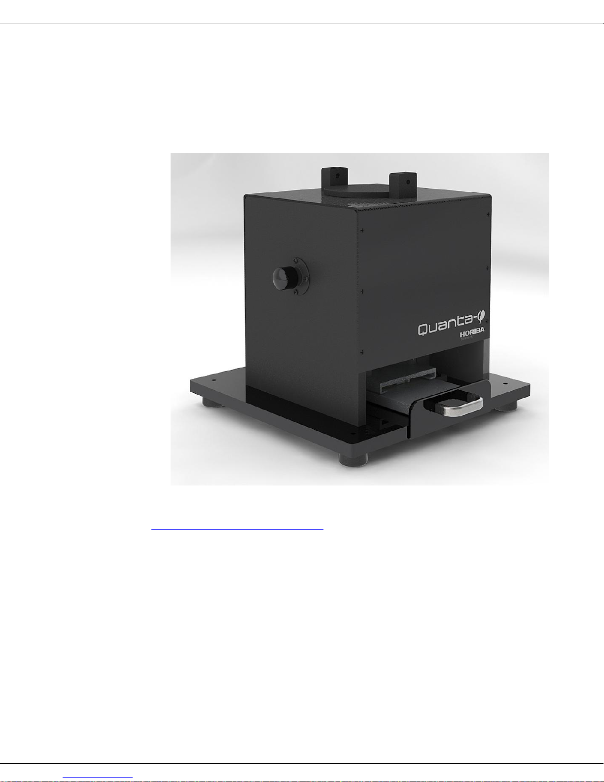
Note:
Keep this and the other reference manuals near the system.
0 : Introduction
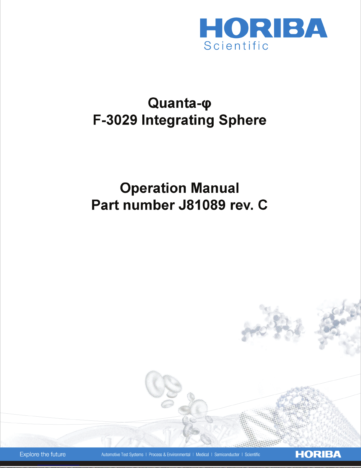
About the Quanta-φ integrating sphere
This manual explains the theoretical and practical issues of operating and maintaining
the Quanta- integrating sphere. The Quanta- is used with the Fluorolog®-3, FluoroMax®-3 and -4, and Fluorolog®-Tau-3 spectrofluorometers to study fluorescence from
solid, powder, thin-film and liquid samples. The main purpose of the Quanta- is the
measurement of photoluminescence quantum yields of such materials.
The Quanta- integrating sphere accessory is external to the spectrofluorometer. Light
from the sample compartment is directed into the sphere via a fiber-optic cable and the
F-3000 Fiber-Optic Adapter, and returned to the sample compartment (and then to the
emission monochromator) via a second fiber-optic cable and the F-3000.
0-1

Quanta-φ rev. C (23 Apr 2010) Introduction
Disclaimer
By setting up or starting to use any HORIBA Jobin Yvon product, you are accepting
the following terms:
You are responsible for understanding the information contained in this document. You
should not rely on this information as absolute or all-encompassing; there may be local
issues (in your environment) not addressed in this document that you may need to address, and there may be issues or procedures discussed that may not apply to your situation.
If you do not follow the instructions or procedures contained in this document, you are
responsible for yourself and your actions and all resulting consequences. If you rely on
the information contained in this document, you are responsible for:
Adhering to safety procedures
Following all precautions
Referring to additional safety documentation, such as Material Safety Data Sheets
(MSDS), when advised
As a condition of purchase, you agree to use safe operating procedures in the use of all
products supplied by HORIBA Jobin Yvon, including those specified in the MSDS
provided with any chemicals and all warning and cautionary notices, and to use all
safety devices and guards when operating equipment. You agree to indemnify and hold
HORIBA Jobin Yvon harmless from any liability or obligation arising from your use or
misuse of any such products, including, without limitation, to persons injured directly
or indirectly in connection with your use or operation of the products. The foregoing
indemnification shall in no event be deemed to have expanded HORIBA Jobin Yvon’s
liability for the products.
HORIBA Jobin Yvon products are not intended for any general cosmetic, drug, food, or
household application, but may be used for analytical measurements or research in
these fields. A condition of HORIBA Jobin Yvon’s acceptance of a purchase order is
that only qualified individuals, trained and familiar with procedures suitable for the
products ordered, will handle them. Training and maintenance procedures may be purchased from HORIBA Jobin Yvon at an additional cost. HORIBA Jobin Yvon cannot
be held responsible for actions your employer or contractor may take without proper
training.
Due to HORIBA Jobin Yvon’s efforts to continuously improve our products, all specifications, dimensions, internal workings, and operating procedures are subject to
change without notice. All specifications and measurements are approximate, based on
a standard configuration; results may vary with the application and environment. Any
software manufactured by HORIBA Jobin Yvon is also under constant development
and subject to change without notice.
Any warranties and remedies with respect to our products are limited to those provided
in writing as to a particular product. In no event shall HORIBA Jobin Yvon be held lia-
0-2

Quanta-φ rev. C (23 Apr 2010) Introduction
ble for any special, incidental, indirect or consequential damages of any kind, or any
damages whatsoever resulting from loss of use, loss of data, or loss of profits, arising
out of or in connection with our products or the use or possession thereof. HORIBA Jobin Yvon is also in no event liable for damages on any theory of liability arising out of,
or in connection with, the use or performance of our hardware or software, regardless
of whether you have been advised of the possibility of damage.
0-3
Quanta-φ rev. C (23 Apr 2010) Introduction
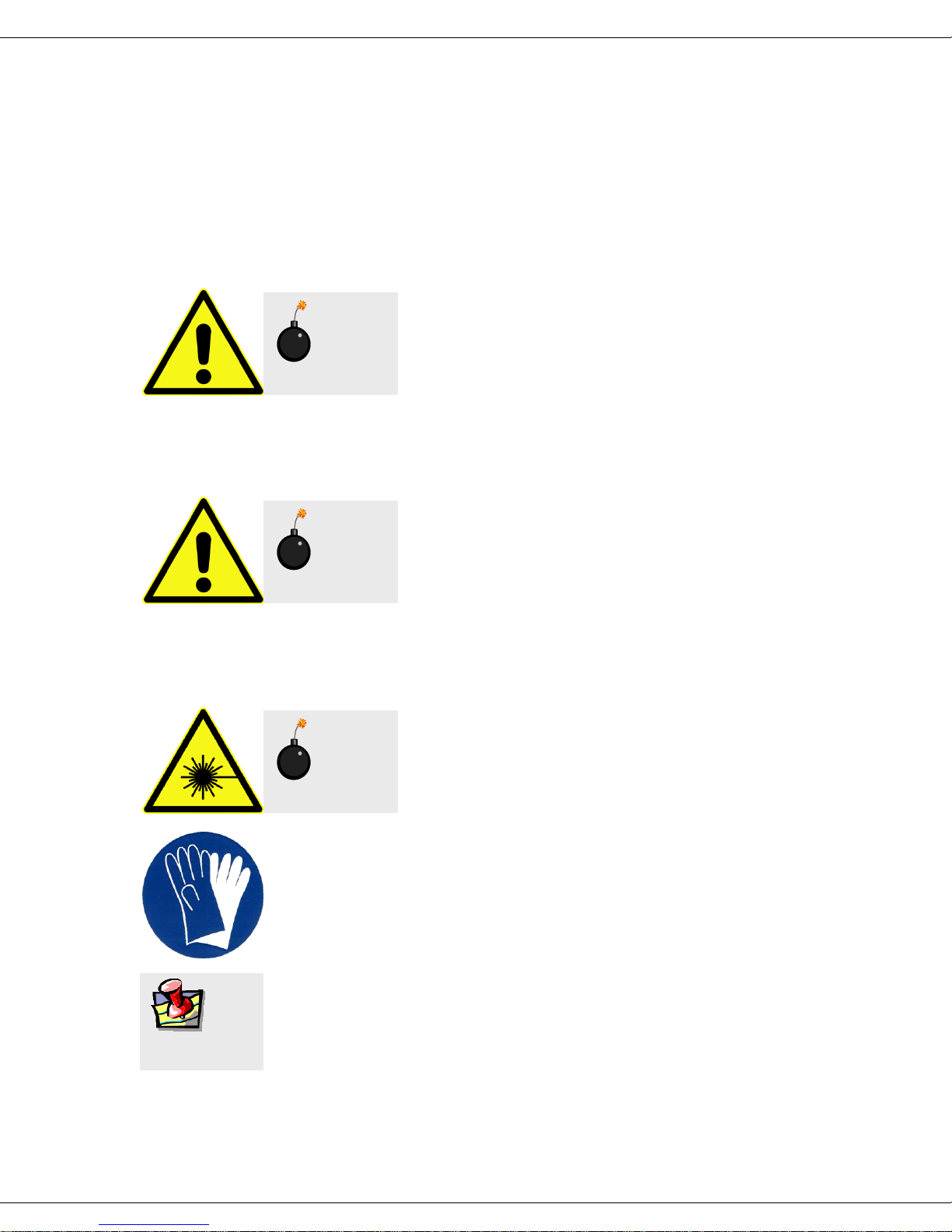
A WARNING notice denotes a hazard. It calls
attention to an operating procedure, practice, or
similar that, if incorrectly performed or adhered
to, could result in personal injury or death. Do
not proceed beyond a WARNING notice until
the indicated conditions are fully understood and
met. HORIBA Jobin Yvon Inc. is not responsible for damage arising out of improper use of the
equipment.
A CAUTION notice denotes a hazard. It calls
attention to an operating procedure, practice, or
similar that, if incorrectly performed or adhered
to, could result in damage to the product. Do not
proceed beyond a CAUTION notice until the
indicated conditions are fully understood and
met. HORIBA Jobin Yvon Inc. is not responsible for damage arising out of improper use of the
equipment.
Intense ultraviolet, visible, or infrared light!
Wear light-protective goggles, full-face shield,
skin-protection clothing, and light-blocking
gloves. Do not stare into light.
Wear protective gloves.
General information is given concerning operation of the equipment.
Note:
Caution:
Caution:
Warning:
Safety summary
The following general safety precautions must be observed during all phases of operation of this instrument. Failure to comply with these precautions or with specific warnings elsewhere in this manual violates safety standards of design, manufacture and in-
tended use of instrument. HORIBA Jobin Yvon assumes no liability for the customer’s
failure to comply with these requirements. Certain symbols are used throughout the text
for special conditions when operating the instruments:
0-4
Quanta-φ rev. C (23 Apr 2010) Introduction
Caution:
This instrument is used in conjunction with ultraviolet light. Exposure to these radiations, even reflected
or diffused, can result in serious, and sometimes irreversible, eye and skin injuries.
Overexposure to ultraviolet rays threatens human health
by causing:
Immediate painful sunburn
Skin cancer
Eye damage
Immune-system suppression
Premature aging
Risks of ultraviolet exposure
Do not aim the UV light at anyone.
Do not look directly into the light.
Always wear protective goggles, full-face shield and skin protection clothing and
gloves when using the light source.
Light is subdivided into visible light, ranging from 400 nm (violet) to 700 nm (red);
longer infrared, ―above red‖ or > 700 nm, also called heat; and shorter ultraviolet
radiation (UVR), ―below violet‖ or < 400 nm. UVR is further subdivided into UV-
A or near-UV (320–400 nm), also called black (invisible) light; UV-B or mid-UV
(290–320 nm), which is more skin penetrating; and UV-C or far-UV (< 290 nm).
Health effects of exposure to UV light are familiar to anyone who has had sunburn.
However, the UV light level around some UV equipment greatly exceeds the level
found in nature. Acute (short-term) effects include redness or ulceration of the skin.
At high levels of exposure, these burns can be serious. For chronic exposures, there
is also a cumulative risk of harm. This risk depends upon the amount of exposure
during your lifetime. The long-term risks for large cumulative exposure include
premature aging of the skin, wrinkles and, most seriously, skin cancer and cataract.
Damage to vision is likely following exposure to high-intensity UV radiation. In
adults, more than 99% of UV radiation is absorbed by the anterior structures of the
eye. UVR can contribute to the development of age-related cataract, pterygium,
photodermatitis, and cancer of the skin around the eye. It may also contribute to
age-related macular degeneration. Like the skin, the covering of the eye or the cornea, is epithelial tissue. The danger to the eye is enhanced by the fact that light can
enter from all angles around the eye and not only in the direction of vision. This is
especially true while working in a dark environment, as the pupil is wide open. The
lens can also be damaged, but because the cornea acts as a filter, the chances are re-
0-5
Quanta-φ rev. C (23 Apr 2010) Introduction
Caution:
UV exposures are not immediately felt. The user may not realize the hazard until it is too late and the
damage is done.
duced. This should not lessen the concern over lens damage however, because cataracts are the direct result of lens damage.
Burns to the eyes are usually more painful and serious than a burn to the skin. Make
sure your eye protection is appropriate for this work. NORMAL EYEGLASSES OR
CONTACTS OFFER VERY LIMITED PROTECTION!
Training
For the use of UV sources, new users must be trained by another member of the laboratory who, in the opinion of the member of staff in charge of the department, is sufficiently competent to give instruction on the correct procedure. Newly trained users
should be overseen for some time by a competent person.
0-6
Quanta-φ rev. C (23 Apr 2010) Introduction
Warning:
Xenon lamps
are dangerous. Please
read the following precautions.
Additional risks of xenon lamps
Among the dangers associated with xenon lamps
are:
Burns caused by contact with a hot xenon lamp.
Fire ignited by hot xenon lamp.
Interaction of other nearby chemicals with intense ultraviolet, visible, or infrared
radiation.
Damage caused to apparatus placed close to the xenon lamp.
Explosion or mechanical failure of the xenon lamp.
Visible radiation
Any very bright visible light source will cause a human aversion response: we either
blink or turn our head away. Although we may see a retinal afterimage (which can last
for several minutes), the aversion response time (about 0.25 seconds) normally protects
our vision. This aversion response should be trusted and obeyed. NEVER STARE AT
ANY BRIGHT LIGHT-SOURCE FOR AN EXTENDED PERIOD. Overriding the
aversion response by forcing yourself to look at a bright light-source may result in permanent injury to the retina. This type of injury can occur during a single prolonged exposure. Excessive exposure to visible light can result in skin and eye damage.
Visible light sources that are not bright enough to cause retinal burns are not necessarily safe to view for an extended period. In fact, any sufficiently bright visible light
source viewed for an extended period will eventually cause degradation of both night
and color vision. Appropriate protective filters are needed for any light source that
causes viewing discomfort when viewed for an extended period of time. For these reasons, prolonged viewing of bright light sources should be limited by the use of appropriate filters.
The blue-light wavelengths (400–500 nm) present a unique hazard to the retina by
causing photochemical effects similar to those found in UV-radiation exposure.
Infrared radiation
Infrared (or heat) radiation is defined as having a wavelength between 780 nm and 1
mm. Specific biological effectiveness ―bands‖ have been defined by the CIE (Commission Internationale de l’Eclairage or International Commission on Illumination) as follows:
IR-A (near IR) (780–1400 nm)
IR-B (mid IR) (1400–3000 nm)
IR-C (far IR) (3000 nm–1 mm)
0-7

Quanta-φ rev. C (23 Apr 2010) Introduction
The skin and eyes absorb infrared radiation (IR) as heat. Workers normally notice excessive exposure through heat sensation and pain. Infrared radiation in the IR-A that
enters the human eye will reach (and can be focused upon) the sensitive cells of the retina. For high irradiance sources in the IR-A, the retina is the part of the eye that is at
risk. For sources in the IR-B and IR-C, both the skin and the cornea may be at risk from
―flash burns.‖ In addition, the heat deposited in the cornea may be conducted to the lens
of the eye. This heating of the lens is believed to be the cause of so called ―glassblow-
ers’ ‖ cataracts because the heat transfer may cause clouding of the lens.
Retinal IR Hazards (780 to 1400 nm): possible retinal lesions from acute high irra-
diance exposures to small dimension sources.
Lens IR Hazards (1400 to 1900 nm): possible cataract induction from chronic lower
irradiance exposures.
Corneal IR Hazards (1900 nm to 1 mm): possible flashburns from acute high irra-
diance exposures.
Who is likely to be injured? The user and anyone exposed to the radiation or xenon
lamp shards as a result of faulty procedures. Injuries may be slight to severe.
0-8

Quanta-φ rev. C (23 Apr 2010) Theory of Operation
2
2
21
coscos
dA
Sπ
θθ
dF
sphere
A
A
rπ
A
F
2
2
2
4
Aπ
ρ
L
i
Φ
M
Aπ
L
i
Φ
1 : Theory of Operation
Introduction
An ideal integrating sphere is designed to integrate light for collection over all emission
angles from the sample. No integrating sphere is ideal, and so there are various approximations required.
Spherical enclosures and radiance
When light hits a diffuse surface, such as the interior of an integrating sphere, radiation
exchange occurs. Imagine an area dA1 that reflects light to another area dA2. We can
write the exchange factor dF, the fraction of energy leaving dA1, traveling a distance S,
and going to dA2.
(1)
For a spherical enclosure, the area dA1 actually exchanges light with an area A2 of definite size. With geometrical considerations, we can integrate the differentials to get
(2)
Equation (2) tells us that the fraction of light F that A2 receives is just A
’s fraction of
2
the sphere’s total surface area. The parameter F is independent of the viewing angle, is
the same when measured from anywhere within the integrating sphere, and is proportional to the area of the sphere.
Radiance, L, is the flux density of light emanating per unit solid angle. For a diffuse
surface receiving an incident flux Φi,
(3)
where A is the area under illumination, ρ is the reflectance, and π is the solid angle from
the surface. The main issue here is the reflectance for an integrating sphere. The reflectance can be rewritten as a simplification of a power series from multiple reflections
within the sphere. Thus we rewrite the radiance as
(4)
1-1
Quanta-φ rev. C (23 Apr 2010) Theory of Operation
fρ
ρ
M
11
τ
te
ρc
d
τ
sphere
ln
1
3
2
where M is a factor called the sphere multiplier. The sphere multiplier takes into account the total fractional area f that the entrance and exit ports occupy (and thus reduce
the reflectance), plus multiple reflections:
For a typical integrating sphere whose ρ ~ 0.95 and f ~ 0.03, M is between 10 and 30.
(5)
Time decay of signal
An incoming signal (such as a rapid fluorescence-decay) can be stretched temporally
because of the multiple diffuse reflections inside an integrating sphere. This can be important for fluorescence lifetime determinations. The impulse response of an integrating
sphere takes the form
where τ is the time constant of the integrating sphere, and is
Equation (6) considers also the diameter of the integrating sphere, d
reflectance, ρ, and the speed of light, c. A typical τ might range from several ns to sev-
eral dozen ns.
(6)
, the average
sphere
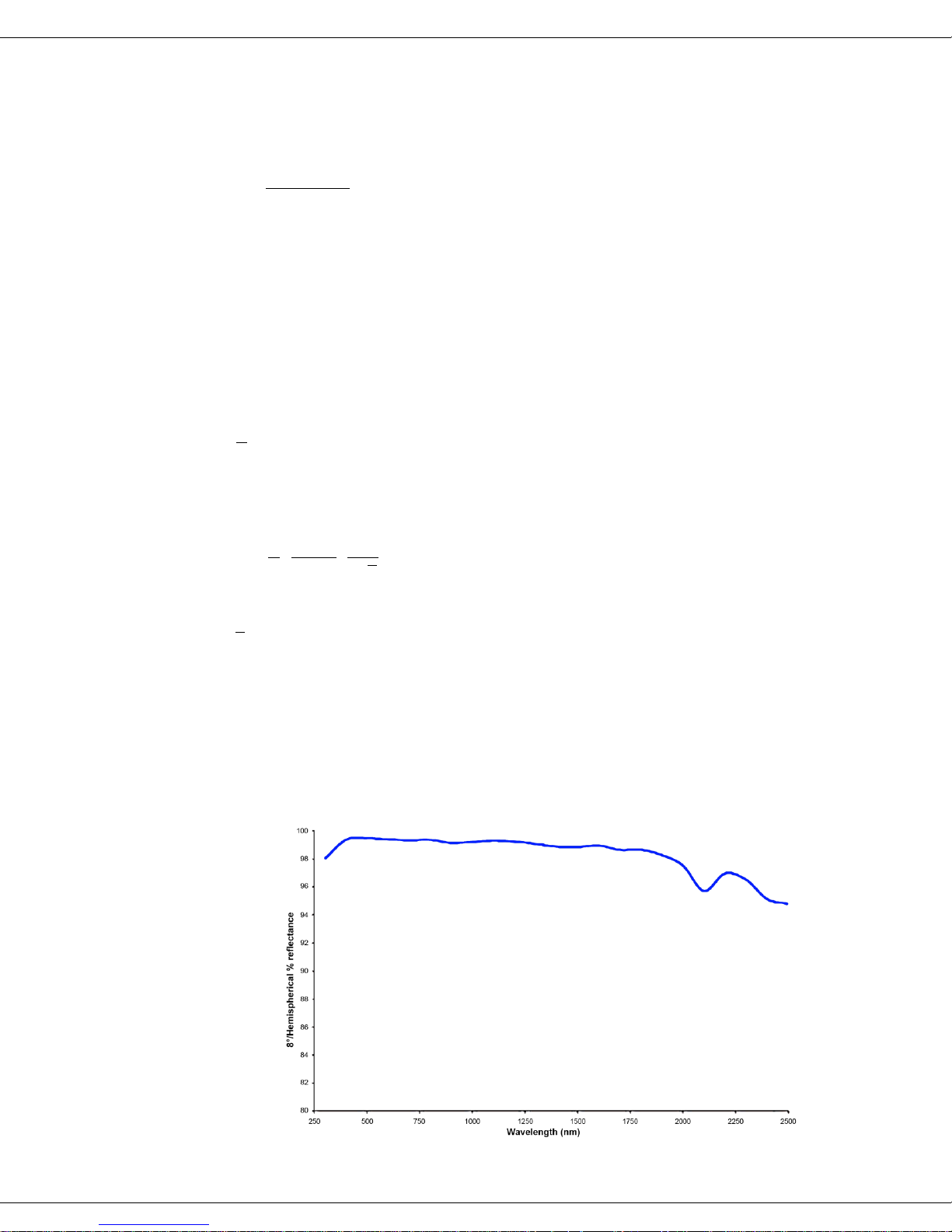
Coating of an integrating sphere
The interior reflective coating of an integrating sphere affects its overall performance.
The interior of the HORIBA Scientific integrating sphere is made from a proprietary
material known as Spectralon®, which has a very wide, flat reflectance of over 95%
from 250 nm to 2.5 μm (see graph below). Thus this integrating sphere is useful
throughout the
spectrofluorome-
ter’s scanning
range, from the
UV through the
near-IR.
1-2

Quanta-φ rev. C (23 Apr 2010) Theory of Operation
b
cb
L
LLA
Photoluminescence quantum yield
An important use of the integrating sphere in conjunction with your spectrofluorometer
is the determination of a sample’s photoluminescence quantum yield. The photoluminescence quantum yield for a particular molecular species is determined by the firstorder rate processes that compete for the excitation energy. The three main processes
can be defined with first-order rate constants, such as kF, the rate constant of fluorescence decay (in units of s–1), kNR, the rate constant of nonradiative decay, and kT, the
rate constant of photochemical energy transfer. Using these three rate constants, the
fluorescence quantum yield φ is defined as
The fluorescence quantum yield is directly related to the fluorescence lifetime τ:
Any increase in the nonradiative decay processes (kNR) related to events such as
quenching and thermal dissipation or energy-transfer (kT) processes—including Förster
Resonance Energy Transfer (FRET)—will decrease both the quantum yield φ and fluorescence lifetime τ. Likewise any decrease in kNR or kT will increase φ and τ.
The multiple randomized, diffused reflections in the integrating sphere eliminate
any isotropic (directional) features of the sample emission from the excited molecular
species. Hence, measurement of polarization is not possible within an integrating
sphere.
Following is a brief description of the theory and recommended procedure for measuring quantum yield using the Quanta-φ integrating sphere.
General approach
For a general approach, not requiring an integrating sphere, see Joseph R. Lakowicz’s
book, Principles of Fluorescence Spectroscopy.1
Theory
The sample is placed in the integrating sphere, and excited with a monochromatic
source of wavelength λ. The film absorbance, A, is
1
Joseph R. Lakowicz, Principles of Fluorescence Spectroscopy, 3rd ed., New York, Springer, 2006, pp.
8–10, 54–55.
(7)
1-3

Quanta-φ rev. C (23 Apr 2010) Theory of Operation
Caution:
Always attenuate or adjust the signal intensities to prevent saturation of the detector. Saturated signals can seriously deteriorate the
measurement precision and accuracy, and possibly damage the detection electronics.
1
cb
ca
a a c
E A E
EE
L A L L
where Lb is the integrated excitation profile when the sample is diffusely illuminated by
the integrating sphere’s surface; and Lc is the integrated excitation profile when the
sample is directly excited by the incident beam.
The quantum yield, υ, is, by definition, photons emitted to photons absorbed:
(8)
where Ec is the integrated luminescence of the film caused by direct excitation, and Eb
is the integrated luminescence of the film caused by indirect illumination from the
sphere. The term La is the integrated excitation profile from an empty integrating sphere
(without the sample, only a blank). Here Ea is the integrated luminescence from an
empty integrating sphere (only a blank).
For integration of function L over the wavelength, λ, the integration limits can be from
10 nm below the excitation wavelength to 10 nm above the excitation wavelength.
The spectra recorded must be background corrected, using a blank sample holder, and
corrected for wavelength dependence of the spectrofluorometer, sampling optics, and
integrating sphere.
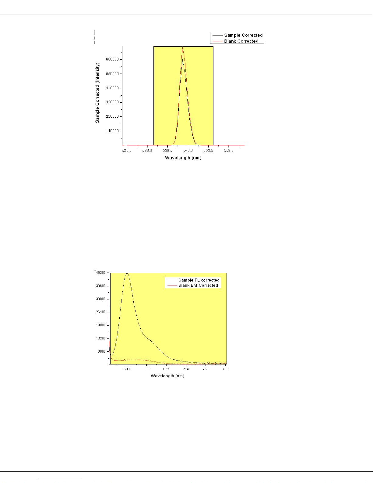
Example
An example is given for rhodamine 101 (see right) in anhydrous ethanol (with a peak
absorbance value of OD = 0.063 at 563 nm) excited
using 545-nm light (OD = 0.035) using 1 nm bandpass
for both excitation and emission.
Using a CCD detector, the scattered 545 nm excitation spectra were recorded for both
the blank cuvette containing only ethanol (red, La), and the sample cuvette (black, Lc).
Integration of the instrument-corrected incident beam’s signal intensities I was performed from 535 to 553 nm for 0.5 s (20 summed accumulations).
1-4
Quanta-φ rev. C (23 Apr 2010) Theory of Operation
553
6
535
2.27954 10
a
L I d
553
6
535
1.9856 10
c
L I d
800
5
553
3.29376 10
a
E I d
800
6
553
2.51648 10
c
E I d
(9)
(10)
Next, the sample and blank’s fluorescence spectral region intensities were measured using a 4-second integration time under otherwise the same instrument conditions as the
La and Lc. Integration of the emission-signal region Ea (blank) and Ec (sample) was
from 553 to 800 nm.
(11)
(12)
1-5

Quanta-φ rev. C (23 Apr 2010) Theory of Operation
65
66
[( )/8]
100%
[(2.51648 10 3.29376 10 ) /8]
100%
2.27954 10 1.9856 10
93.01%
ca
ac
EE
LL
Because the integration time constant used to collect Ea and Ec was 8 times longer than
for La and Lc, we need to divide the difference between Ea and Ec by 8 to calculate the
quantum yield, υ, below using the four parameters Ec, Ea, La, and Lc,.
This υ is slightly lower compared to some literature reports for rhodamine 101 in acidifed ethanol (~ 96–99%) primarily due to the anhydrous ethanol used as the solvent.
Error-propagation analysis
In addition to the calculation of υ, the Quanta-φ software performs an error-propagation
analysis to help evaluate when signal levels are not properly balanced. This may occur
with dilute concentrations of the sample, or when samples exhibit very low quantum efficiency. The error propagation is based on the Poissonian statistics of photon-counting,
where the standard deviation σ is equal to the square-root of the photon-count value,
i.e.,
The error propagation is performed in a stepwise manner.
First, find the standard deviations for Ea, Ec, La, and L
,
and
.
, respectively as
c
Second, evaluate the standard deviation of the numerator num = [(Ec – Ea)/8] of the υ
equation (considering the constant factor of 8 in the integration time) as
Then evaluate the standard deviation of the denominator den = (La – Lc), as
,
Propagation of the respective relative (σ
) and absolute errors (σ
rel
) of υ is as follows:
abs
1-6

Quanta-φ rev. C (23 Apr 2010) Theory of Operation
For the example given above for rhodamine 101 (υ = 93.01%), σ
= 0.007 and σ
rel
abs
=
0.654 %.
Consider that:
These values can be used to diagnose trends in the precision and accuracy of , es-
pecially when evaluated under conditions where the sample concentration or quantum efficiency is being systematically varied. An example is with a quenching experiment or when titrating the sample concentration to minimize reabsorption (inner
filter) effects.
The error-propagation routine is normalized to the La and Lc integration conditions
as a general rule. This is because the Ea and Ec values (which are typically less intense) are normally collected under conditions of longer integration time or higher
excitation power so that these values must be divided by a constant factor in the equation for υ.
The largest absolute source of error in the υ measurement is likely to be in the larg-
er La and Lc values. Therefore HORIBA Scientific recommends that you carefully
consider the required integration time and excitation-power conditions for the Ea
and Ec values to prevent the larger noise-levels in La and Lc from ―swamping out‖
the smaller fluorescence area signal value. This is a particularly important prob-
lem with the ratiometric nature of the equation, because the larger source of
error is in the denominator.
Self-absorption and inner-filter effects
The measurement of υ, as an absolute value, is strongly influenced by the sample concentration. Relative changes and observed values of υ can be easily complicated by
concentration-related artifacts. Because υ is determined by the number of photons absorbed, the concentration must be measured under the ―Beer-Lambert‖ criterion of a linear relationship between OD and sample concentration.
One important effect of increasing sample concentration is ―self-absorption‖, a depression in the bluer edge of the emission spectral region, where it overlaps with the redder
edge of the excitation or absorbance spectrum.
HORIBA Scientific recommends the following practical considerations to avoid selfabsorption:
Adjust the sample concentration so that, when plotting absorption (A) or optical
density (OD) against concentration, a linear plot appears. Generally this occurs at
the λ
When possible, make multiple measurements while varying the sample concentra-
tion (OD), to determine if (and when) observed υ and Ec area fall in a linear region
when plotted against sample concentration or OD.
Plot the ―normalized‖ Ec spectral areas, and evaluate their integrated areas relative
to the sample OD, to determine if the blue edges are depressed in a manner systematically related to the OD. For compounds with υ < 100%, and narrow Stokes
shifts between the excitation spectrum and emission spectrum, the relative areas
when OD < 0.1, and better around 0.05.
peak
1-7
Quanta-φ rev. C (23 Apr 2010) Theory of Operation
will be directly related to the measured values. For samples with high quantum
yields (like rhodamine 101), however, or with large Stokes shifts between excitation and emission spectra (like quinine sulfate), re-absorbance effects are significantly smaller.
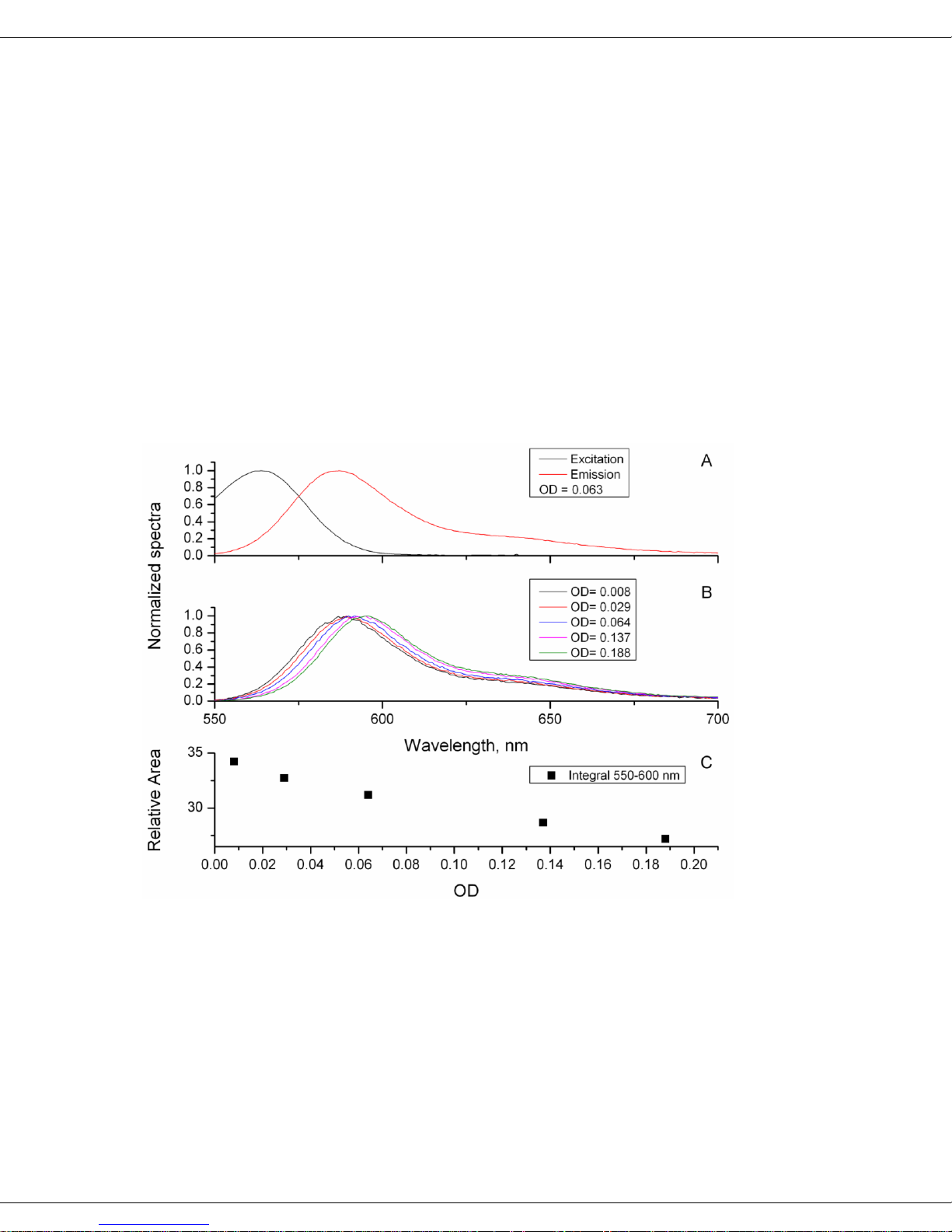
The following figures provide examples how increasing concentration and absorbance
affect emission spectra of rhodamine 101 in anhydrous ethanol, and quinine sulfate in
0.1 N H2SO4, as measured in the Quanta-υ. The top plots (A) for both figures exhibit
the normalized excitation (black) and emission (red) spectra to illustrate the overlapping regions responsible for self-absorption. Clearly the overlap is much larger in rhodamine 101 than in quinine sulfate. The middle plots (B) show the normalized emission
spectra at particular ODs, revealing self-absorption. Again, the rhodamine 101 spectra
are systematically red-shifted as OD increases (from self-absorption). Qunine sulfate,
however, shows little or no change in the emission spectrum as the OD changes. The
lower plots (C) reinforce the visual observations in plots A and B, by showing the relative area. Integrals decrease as OD rises for rhodamine 101, but there is no change in
quinine sulfate.
Influence of OD on fluorescence emission of rhodamine 101 dissolved in anhydrous
ethanol.
1-8
Quanta-φ rev. C (23 Apr 2010) Theory of Operation
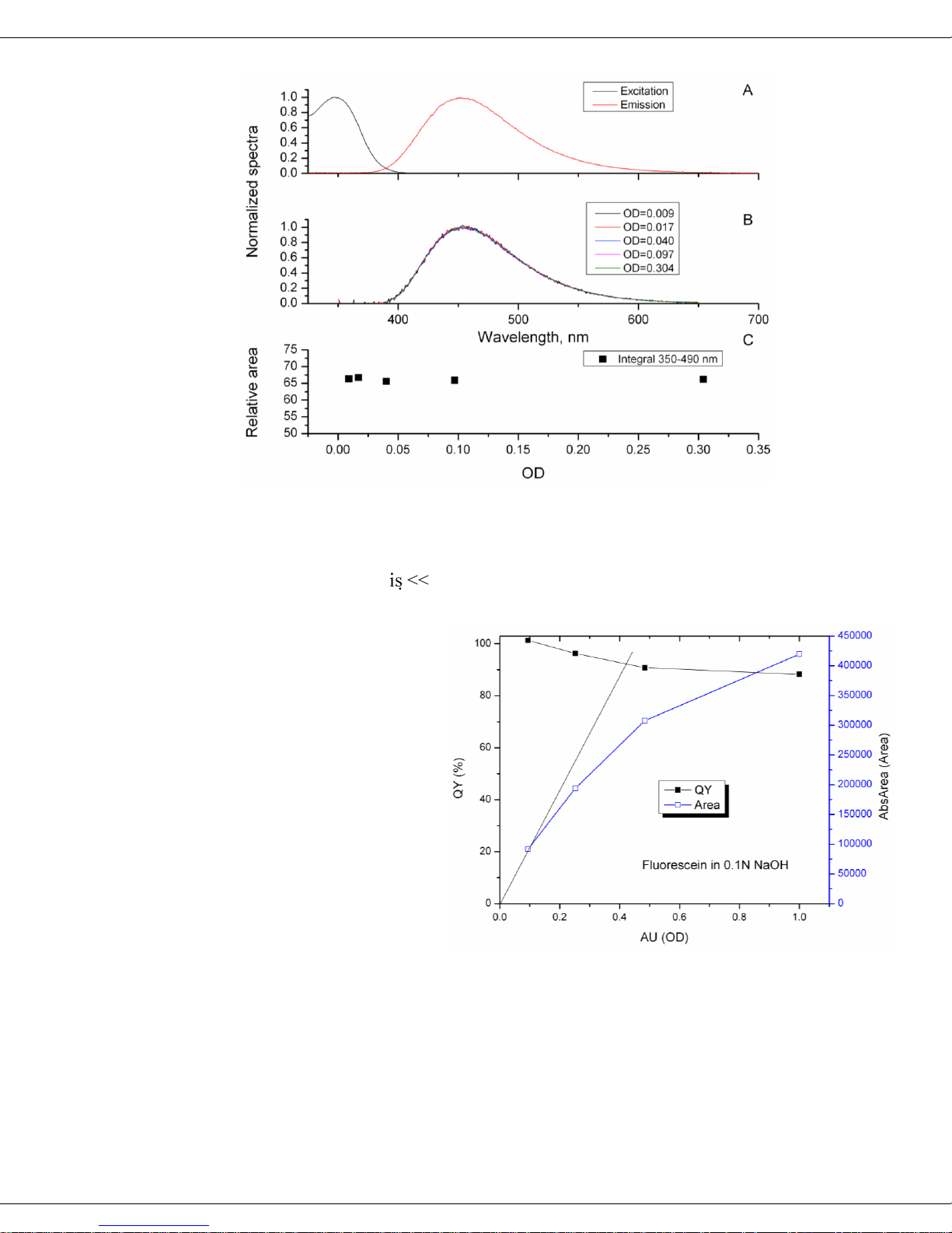
Influence of OD on fluorescence emission of quinine sulfate dissolved in 0.1 N H2SO4.
In both compounds there is no correlation of with concentration because rhodamine
101 has a υ ≈ 93% and quinine sulfate ( ≈ 55%) shows no re-absorption. Yet when the
sample’s intrinsic υ 100 % and self-absorption is strong, the measured υ will be
influenced in proportion to the absorbance (OD) of the sample.
In contrast to rhodamine
101 and quinine sulfate,
the figure to the right depicts the observed relationships between the integrated fluoresence area,
the absorbance, and quantum yield (%) of fluorescein in 0.1 N NaOH.
Clearly as the OD increases beyond 0.1 units,
the relationship between
the fluorescence area
(hollow symbols) and
quantum yield (filled
symbols) becomes increasingly non-linear. Likewise the observed quantum yield becomes depressed with increasing OD, consistent with the inner-filter effects.
Similar to the fluorescein data above, self-absorption is also a problem with many solid
samples and powders whose ODs cannot easily be determined. As with liquid samples,
in solid and powder samples, when possible, HORIBA Scientific advises you to vary
1-9

Quanta-φ rev. C (23 Apr 2010) Theory of Operation
the main chromophore’s concentration systematically to evaluate the self-absorbance
properties of the emission. In powder samples, for instance, pulverize and homogenize
the chromophoric sample with a non-luminescent powder such as barium sulfate, in order to dilute the solid. The principle is similar to that for liquids, in that the sample is
diluted to vary and minimize self-absorption at the surface. The solid dilution also
serves to dilute the chromophoric sample to the point where its light-scattering properties are primarily determined by the surrounding non-luminescent powder. This is important because non-luminescent powder—when similarly pulverized and homogenized—may be used as the blank sample. In powder measurements, homogenization of
the particle-size and light-scattering properties (that is, matching the sample and blank)
is vital to acquiring precise and accurate values for υ.
1-10
Quanta-φ rev. C (23 Apr 2010) Theory of Operation
Line of purples
Blue
apex
Red
apex
Green
apex
White
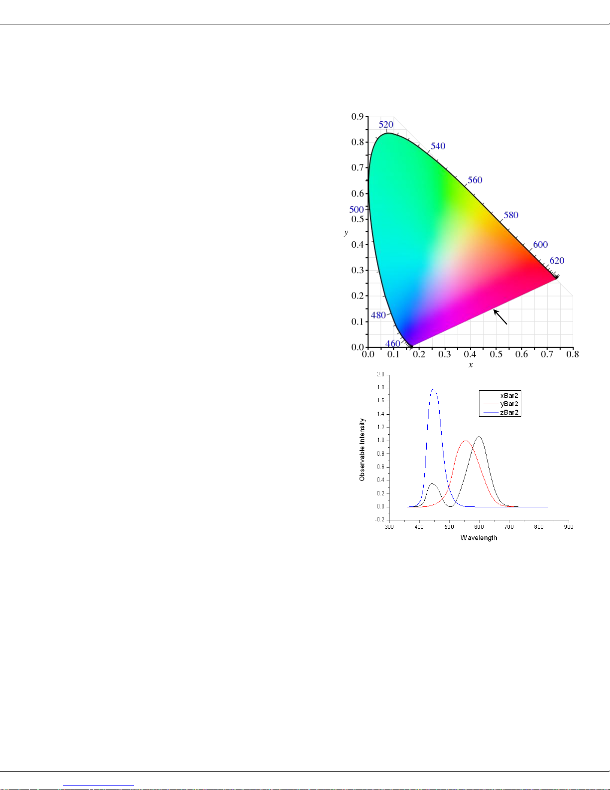
Calculation and evaluation of chromaticity
Theory
The Quanta-φ software automatically
calculates and presents the numerical
and graphical coordinate information
for the spectral region (Ec – Ea) dealing with the chromaticity observable
indices CIE 1931 and CIE 1976. The
chromaticity indices provide a means
for comparing the observed color (or
tint) of the luminescence relative to
the human visual perception of color.
As displayed in the figure on the
right, relative to the CIE 1931 index
plot, the boundary area outlines all
potential hues visible to the human
eye.
The chromaticity indices are based on
the overlapping regions of the normalized luminescence emission spectrum,
with each of the three spectral profiles
depicted in the figure on the right.
The regions of spectral overlap for the
luminescence emission spectrum is evaluated by calculating the sum-product
of the emission spectrum with each of
three observable profiles, namely, xBar,
yBar and zBar. The observable profiles
are related to the three visual sensorycell responses in the human eye, namely, the red (xBar), green (yBar) and blue (zBar).
Note that the red profile also includes a portion of the blue spectral region.
Calculations
The Quanta-φ calculations for CIE 1931 and CIE 1976 proceed as follows.
First the emission spectral regions from 360 nm–800 nm for Ec and Ea are interpo-
lated to 1-nm intervals, and the spectral curve of the blank (Ea) is subtracted from
the sample (Ec).
Then the resultant blank-subtracted sample spectral profile is converted from pho-
ton units to power units, by division of each intensity point by the wavelength value
in nm at which it was measured.
1-11

Quanta-φ rev. C (23 Apr 2010) Theory of Operation
The resultant sample power spectrum is then used to calculate three sum-product
values, namely, CIE_TX, CIE_TY and CIE_TZ, from the observable intensity spectra xBar, yBar and zBar, respectively.
For the CIE 1931 index, the following two coordinates are calculated,
The coordinates x and y are plotted graphically inside the CIE 1931 boundary area,
which is defined numerically for the x coordinate at each wavelength value, λ,
and for the y coordinate at each wavelength value, λ
where xBarλ, yBarλ and zBarλ are the intensity values from the three observable profiles
at wavelength λ. The corresponding xBA λ and yBA λ values are plotted against each
other to generate the semielliptical two-dimensional area-boundary plot for CIE 1931
(blue, left) as shown in the sample plot for rhodamine 101 in anhydrous ethanol in the
screenshot on the next page.
For the CIE 1976 index, two coordinates are calculated as follows:
The coordinates u′ and v′ are plotted graphically inside the CIE 1976 boundary area,
which is calculated from the xBA λ and yBA λ values for the u′ coordinate at each wavelength value, λ,
and for the v′ coordinate at each wavelength value, λ
1-12
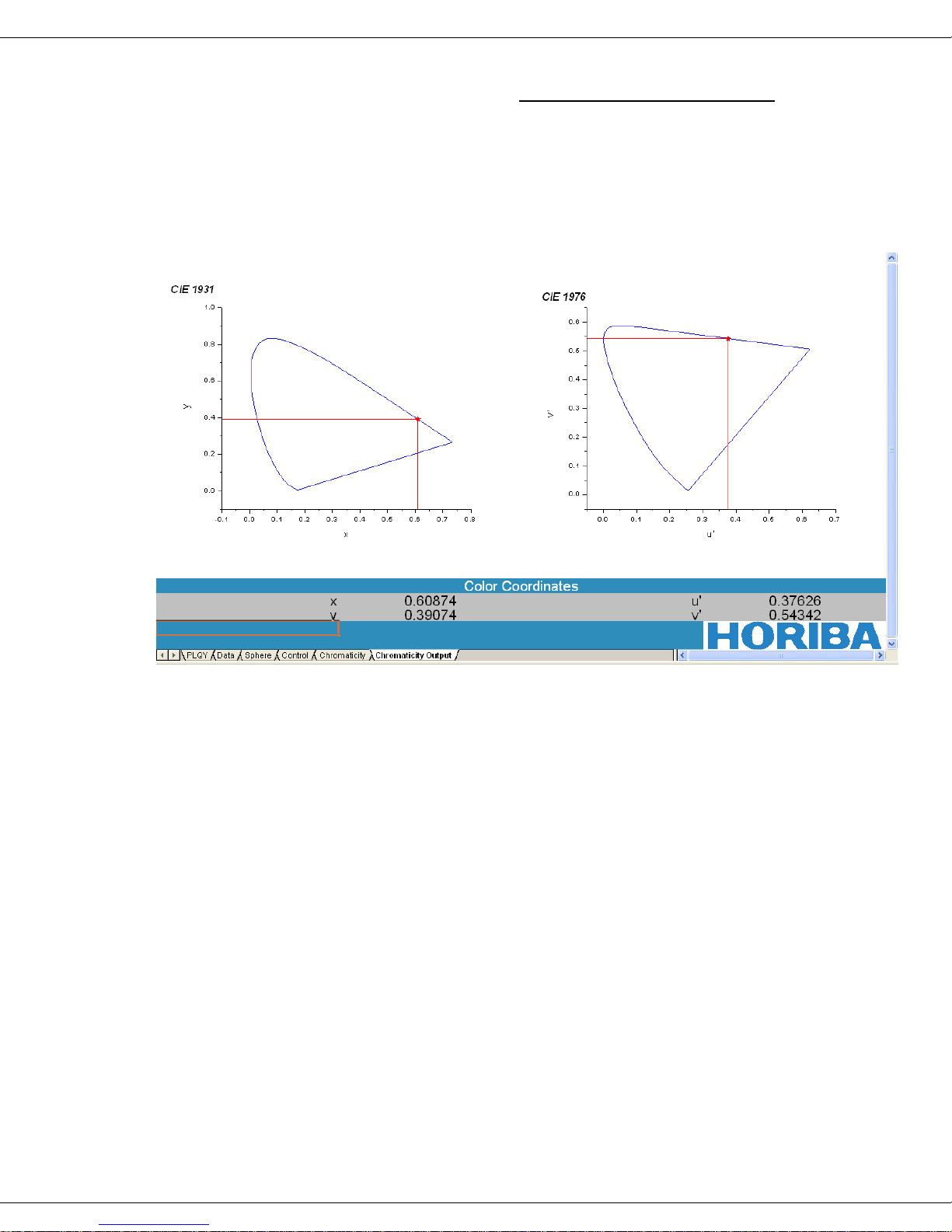
Quanta-φ rev. C (23 Apr 2010) Theory of Operation
The corresponding u′BA λ and v′BA λ values are plotted against each other to generate
the closed, semielliptical two-dimensional area-boundary plot for CIE 1976 (blue,
right) as shown in the sample plot for rhodamine 101 in anhydrous ethanol in the
screenshot below.
1-13
Quanta-φ rev. C (23 Apr 2010) Theory of Operation
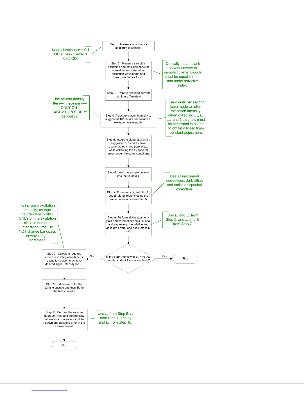
Flowchart of method for data-acquisition
1-14

Quanta-φ rev. C (23 Apr 2010) Theory of Operation
Additional references:
―An improved experimental determination of external photoluminescence quantum ef-
ficiency‖, J.C. deMello, H.F. Wittmann, and R.H. Friend, Adv. Mater. 9, 230 (1997).
―Measurement of Solid-State Photoluminescence Quantum Yields of Films using a
Fluorimeter‖, L.-O. Pålsson, A.P. Monkman, Adv. Mater. 14(10), 2002, 757–758.
―Absolute Measurements of Photoluminescence Quantum Yields of Solutions Using an
Integrating Sphere‖, L. Porrès, A. Holland, L.-O. Pålsson, A.P. Monkman, C. Kemp,
and A. Beeby, J. Fluorescence, 16, 2006.
1-15

Quanta-φ rev. C (23 Apr 2010) Theory of Operation
1-16
 Loading...