Honeywell HMC1055 User Manual

Download

查询HMC1055供应商

HMC1055

Advance Information SENSOR PRODUCTS

3-AXIS COMPASS SENSOR SET

Features

x 3 Precision Sensor Components x 2-Axis Magnetoresistive Sensor for X-Y Axis

Earth’s Field Detection

x 1-Axis Magnetoresistive Sensor for Z-Axis Earth’s

Field Detection

x 2-Axis Accelerometer for 60° Tilt Compensation x 2.7 to 5.5 volt Supply Range x 3-Axis Compass Reference Design Included

Product Description

The Honeywell HMC1055 3-Axis Compass Sensor Set combines the popular HMC1051Z one-axis and the HMC1052 two-axis magneto-resistive sensors plus a 2axis MEMSIC MXS3334UL accelerometer in a single kit. By combining these three sensor packages, OEM compass system designers will have the building blocks needed to create their own tilt compensated compass designs using these proven components.

The HMC1055 chip set includes the three sensor integrated circuits and an application note describing sensor function, a reference design, and design tips for integrating the compass feature into other product platforms.

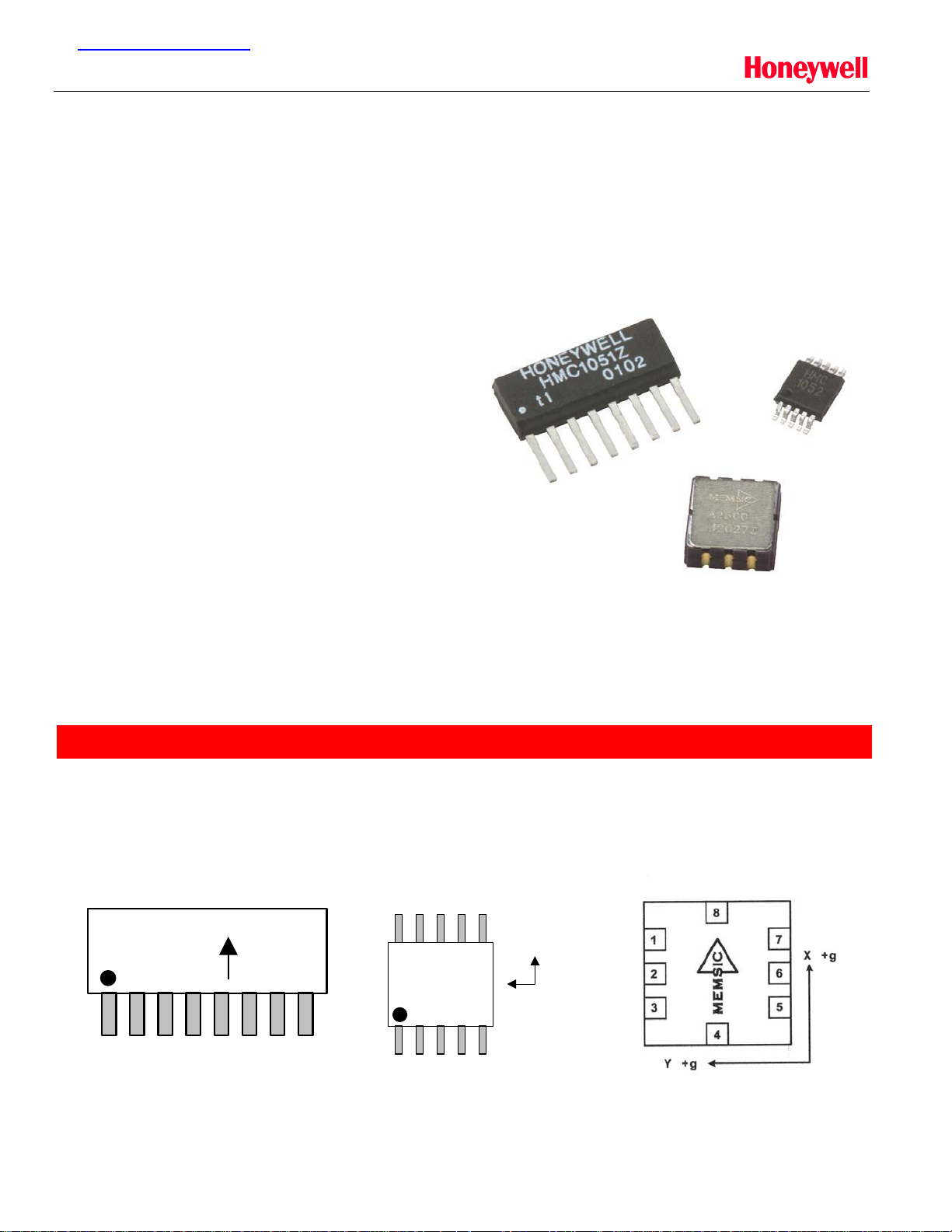
DIAGRAMS

Pinouts (top view)

HONEYWELL

HMC1051Z

HMC 1052

678910

12345678

12345

Solid State Electronics Center • www.magneticsensors.com • (800) 323-8295 • Page 1

HMC1055

Advance Information SENSOR PRODUCTS SPECIFICATIONS – MAGNETIC SENSORS HMC1051Z, HMC1052

Characteristics Conditions* Min Typ Max Units

Bridge Elements

Supply Vbridge referenced to GND 1.8 2.5 20 Volts

Resistance Bridge current = 1mA 800 1000 1500 ohms

Field Range Full scale (FS) – total applied field -6 +6 gauss

Sensitivity Set/Reset Current = 0.5A 0.8 1.0 1.2 mV/V/gauss

Bridge Offset Offset = (OUT+) – (OUT-)

Field = 0 gauss after Set pulse

Bandwidth Magnetic signal (lower limit = DC) 5 MHz

Noise Density @ 1kHz, Vbridge=5V 50 nV/sqrt Hz

Resolution 50Hz Bandwidth, Vbridge=5V 120

Disturbing Field Sensitivity starts to degrade.

Use S/R pulse to restore sensitivity.

Max. Exposed

No perming effect on zero reading 10000 gauss

Field

Operating

Ambient -40 125 °C

Temperature

Storage

Ambient, unbiased -55 150 °C

Temperature

Sensitivity

Tempco

Bridge Offset

Tempco

Bridge Ohmic

TA=-40 to 125°C, Vbridge=5V

=-40 to 125°C, Ibridge=5mA

TA=-40 to 125°C, No Set/Reset

=-40 to 125°C, With Set/Reset

Vbridge=5V, TA=-40 to 125°C 2100 2500 2900 ppm/°C

Tempco

Sensitivity Ratio of

TA=-40 to 125°C 95 101 105 %

X,Y Sensors

(HMC1052 Only)

X,Y sensor

Sensitive direction in X and Y sensors 0.01 degree

Orthogonality

(HMC1052)

Linearity Error Best fit straight line

± 1 gauss

± 3 gauss

± 6 gauss

Hysteresis Error 3 sweeps across ±3 gauss 0.06 %FS

Repeatability Error 3 sweeps across ±3 gauss 0.1 %FS

* Tested at 25°C except stated otherwise.

-1.25 ±0.5 +1.25 mV/V

Pgauss

20 gauss

-3000 -2700

-2400 ppm/°C

-600

±500

ppm/°C

±10

0.1

0.5

%FS

1.8

Solid State Electronics Center • www.magneticsensors.com • (800) 323-8295 • Page 2

HMC1055

Advance Information SENSOR PRODUCTS SPECIFICATIONS – MAGNETIC SENSORS HMC1051Z, HMC1052

Characteristics Conditions* Min Typ Max Units

Set/Reset Strap

Resistance Measured from S/R+ to S/R- 3 4 5 ohms

Current 0.1% duty cycle, or less,

2Psec current pulse

Resistance

Tempco

Offset Straps

Resistance Measured from OFFSET+ to OFFSET- 12 15 18 ohms

Offset

Constant

Resistance

Tempco

* Tested at 25°C except stated otherwise.

SPECIFICATIONS – ACCELEROMETER MXS3334UL Characteristics Conditions* Min Typ Max Units

Sensor Input

Range ±1 g

Non-Linearity Best fit straight line 0.5 1.0 % of FS

Alignement Error ±1.0 degree

Transverse

Sensitivity

Digital Outputs Vdd = 5.0 volts 19.00 20.00 21.00

Change Over

Temperature

Resistance TA= -40 to 125°C 3900 ppm/°C

Zero g Bias Level

0 g Offset -0.1 0.00 +0.1 g

0 g Duty Cycle 48 50 52 % Duty Cycle

0 g Offset Over

Temperature

Performance

Noise Density rms 0.2 0.4 mg/sqrt-Hz

Frequency

Response

Tested at 25°C except stated otherwise.

(available on die)

Field applied in sensitive direction

(Each Axis)

Compensated (-40°C to +105°C)

(Each Axis)

TA= -40 to 125°C 3700 ppm/°C

DC Current

TA= -40 to 125°C 3900 ppm/°C

-40°C, Uncompensated

+105°C, Uncompensated

' from 25°C

' from 25°C, based on 20%/g

3dB Bandwidth 25 Hz

0.4 0.5 4 Amp

10 mA/gauss

±2.0 %

%Duty

Cycle/g

+100 %

-50

< 3.0

±0.75

±0.015

mg/°C

%/°C

Solid State Electronics Center • www.magneticsensors.com • (800) 323-8295 • Page 3

HMC1055

Advance Information SENSOR PRODUCTS MXS3334UL SPECIFICATIONS

Characteristics Conditions* Min Typ Max Units

Voltage Reference

Vref Vdd = 2.7 to 5.0 2.4 2.5 2.65 volts

Change Over

Temperature

Current Drive

Source 100

Capability

Self Test

Continuous

Voltage Under

Vdd = 5.0 volts, D

Vdd = 2.7 volts, D

OUTX

and D

OUTY

Failure

Digital Outputs

OUTX

and D

Normal Range Vdd = 5.00 volts

)

OUTY

Vdd = 2.7 volts

0.1

Current Source or Sink (Vdd =2.7 to 5.0v) 100

Rise/Fall Time Vdd = 2.7 to 5.0 volts 90 100 110

Turn-On Time Vdd = 5.0 volts

Vdd = 2.7 volts

Power Supply

Operating Voltage

2.7 5.25 volts

Range

Supply Current Vdd = 5.0 volts

Vdd = 2.7 volts

3.0

4.0

Temperature

Operating Range -40 +105 °C

Storage Range -65 +150 °C

Tested at 25°C except stated otherwise.

0.1 mV/°C

5.0

volts

2.7

4.9

volts

2.6

Ksec

100

3.6

4.9

4.2

5.8

msec

Pin Configurations (Arrow indicates direction of applied field that generates a positive output voltage after a SET pulse.)

HMC1051

Vcc

(3)

HMC1051

BRIDGE A BRIDGE B

Vo+(A)

Solid State Electronics Center • www.magneticsensors.com • (800) 323-8295 • Page 4

GND Plane

(2)

Vo-(A)

S/R+

(6)

(8)

Set/Reset Strap

(4)

GND1(B)

(1)

S/R-

(7)

GND2(B)

(5)

HMC1051Z Pinout

HONEYWELL

HMC1051Z

12345678

HMC1055

Advance Information SENSOR PRODUCTS

HMC1052

MXD3334UL

(7)

Sck

(optional)

Vcc

(5)

HMC1052

BRIDGE A BRIDGE B

GND2

OUT-

(10)

GND2

(9)

CLK

Heater

Control

GND1

(3)

S/R+

(6)

Oscillator

OUT+

Internal

(4)

Set/Reset Strap

OUT-

(7)

Continous

Self Test

GND

(1)

S/R-

(8)

Temperature

Reference

Sensor

Voltage

OUT+

(2)

HMC1052 Pinout

678910

HMC

1052

12345

(1)

OUT

(6)

REF

X +g

Low Pass

Gnd

Low Pass

Filter

Low Pass

Filter

(4)(3)(8)

(5)

OUTX

(2)

OUTY

2-AXIS

SENSOR

X axis

Factory Adjust

Offset & Gain

Y axis

Pin Descriptions

HMC1051Z

Pin Name Description

1 GND1(B) Bridge B Ground 1 (normally left open) 2 Vo+(A) Bridge Output Positive 3 Vcc Bridge Positive Supply 4 GND Plane Bridge Ground (substrate) 5 GND2(B) Bridge B Ground 2 (normally left open) 6 S/R+ Set/Reset Strap Positive 7 S/R- Set/Reset Strap Negative 8 Vo-(A) Bridge Output Negative

Y +g

MEMSIC

Top View

Solid State Electronics Center • www.magneticsensors.com• (800) 323-8295•Page 5

HMC1055

Advance Information SENSOR PRODUCTS

HMC1052

Pin Name Description

1 GND Bridge B Ground 2 OUT+ Bridge B Output Positive 3 GND1 Bridge A Ground 1 4 OUT+ Bridge B Output Positive 5 Vcc Bridge Positive Supply 6 S/R+ Set/Reset Strap Positive 7 OUT- Bridge B Output Negative 8 S/R- Set/Reset Strap Negative 9 GND2 Bridge A Ground 2

10 OUT- Bridge A Output Negative

MXD3334UL

Pin Name Description

1T 2D

OUT

OUTY

3 Gnd Ground 4V 5D 6V

OUTX

ref

7 Sck Optional External Clock 8V

Temperature (Analog Voltage) Y-Axis Acceleration Digital Signal

Analog Supply Voltage X-Axis Acceleration Digital Signal

2.5V Reference

Digital Supply Voltage

Package Dimensions

HMC1051Z

HMC1052

Symbol Millimeters

Min Max

B D E

1.371 1.728

0.101 0.249

0.355 0.483

9.829 11.253

3.810 3.988

1.270 ref

6.850 7.300

0.381 0.762

Symbol Millimeters

Min Max

B D

- 1.10

0.05 0.15

0.15 0.30

2.90 3.10

0.50 BSC

4.75 5.05

0.95 BSC

Inches x 10E-3

Min Max

54 68 4 10

14 19 387 443 150 157

50 ref

270 287

15 30

Inches x 10E-3

Min Max

- 43

2.0 5.9

5.9 11.8

114 122

2.0 BSC

187 199

37.4

Solid State Electronics Center • www.magneticsensors.com • (800) 323-8295 • Page 6

HMC1055

Advance Information SENSOR PRODUCTS

MXS3334UL

Application Notes

The HMC1055 Chipset is composed of three sensors packaged as integrated circuits for tilt compensated electronic compass development. These three sensors are composed of a Honeywell HMC1052 two-axis magnetic field sensor, a Honeywell HMC1051Z one-axis magnetic sensor, and the Memsic MXS3334UL two-axis accelerometer. Traditionally, compassing is done with a two-axis magnetic sensor held level (perpendicular to the gravitational axis) to sense the horizontal vector components of the earth’s magnetic field from the south pole to the north pole. By incorporating a third axis magnetic sensor and the two-axis accelerometer to measure pitch and roll (tilt), the compass is able to be electronically “gimbaled” and can point to the north pole regardless of level.

The HMC1052 two-axis magnetic sensor contains two Anisotropic Magneto-Resistive (AMR) sensor elements in a single MSOP-10 package. Each element is a full wheatstone bridge sensor that varies the resistance of the bridge magneto-resistors in proportion to the vector magnetic field component on its sensitive axis. The two bridges on the HMC1052 are orientated orthogonal to each other so that a two-dimensional representation of an magnetic field can be measured. The bridges have a common positive bridge power supply connection (Vb); and with all the bridge ground connections tied together, form the complete two-axis magnetic sensor. Each bridge has about an 1100-ohm load resistance, so each bridge will draw several milli-amperes of current from typical digital power supplies. The bridge output pins will present a differential output voltage in proportion to the exposed magnetic field strength and the amount of voltage supply across the bridge. Because the total earth’s magnetic field strength is very small (~0.6 gauss), each bridge’s vector component of the earth’s field will even be smaller and yield only a couple milli-volts with nominal bridge supply values. An instrumentation amplifier circuit; to interface with the differential bridge outputs, and to amplify the sensor signal by hundreds of times, will then follow each bridge voltage output.

The HMC1051Z is an additional magnetic sensor in an 8-pin SIP package to place the sensor silicon die in a vertical orientation relative to a Printed Circuit Board (PCB) position. By having the HMC1052 placed flat (horizontal) on the PCB and the HMC1051Z vertical, all three vector components of the earth’s magnetic field (X, Y, and Z) are sensed. By having the Z-axis component of the field, the electronic compass can be oriented arbitrarily; and with a tilt sensor, perform tilt-compensated compass heading measurements as if the PCB where perfectly level.

Solid State Electronics Center • www.magneticsensors.com • (800) 323-8295 • Page 7

HMC1055

Advance Information SENSOR PRODUCTS

C1 150P

VCC

VEE

VCC

VEE

Vdd

150P

Vdd

X1 LMV324M

LMV324M

C2 150P

150P

Vdd

X2 LMV324M

LMV324M

Vref

0.1U

Vdd

R12

R12 10K

10K

R13

R13 10K

10K

R10

R10 10

DO0

MICRO-

CONTROLLER

VDD

AN0

AN1

AN2

AN3

GND

DI0

DI1

SCK

RXD

TXD

R1A6R2A

R3A R4A

HMC1052

R1B11R2B

R3B R4B

Rsr1

Rsr1 4

Vdd

1.00MEG

4.99K

Vref

R9 220

220

1.00MEG

4.99K

C4 1U

Vref

X4 IRF7509P

IRF7509P X5

X5 IRF7509N

IRF7509N

R18

1.00MEG

R20

1.00MEG

VCC

VEE

C5 150P

150P

Vdd

X3 LMV324M

LMV324M

Rsr2

Rsr2 4

HMC1051Z

R14Z21R15Z

R16Z R17Z

0.22U

Vdd

R19

4.99K

R21

4.99K

Solid State Electronics Center • www.magneticsensors.com • (800) 323-8295 • Page 8

VDAVDD

VREF

DOUTY

MXS3334UL

TOUT

DOUTX

GND

Figure 1

SCK

3-Axis Compass Reference Design

HMC1055

Advance Information SENSOR PRODUCTS

The MXS3334UL is a two-axis accelerometer in an 8-pin LCC package that provides a digital representation of the earth’s gravitational field. When the MXS3334UL is held level and placed horizontally on a PCB, both digital outputs provide a 100 Hz Pulse Width Modulated (PWM) square wave with a 50 percent duty cycle. As the accelerometer is pitched or rolled from horizontal to vertical, the Doutx and Douty duty cycles will shift plus or minus 20% of its duty from the 50% center point.

The reference design in Figure 1 shows a reference design incorporating all three sensor elements of the HMC1055 chipset for a tilt compensated electronic compass operating from a 5.0 volt regulated power supply described as Vdd. The HMC1052 sensor bridge elements A and B are called out as R1A, R2A, R3A, R4A, and R1B, R2B, R3B, R4B respectively; and create a voltage dividing networks that place nominally 2.5 volts into the succeeding amplifier stages. The HMC1051Z sensor bridge elements R14Z, R15Z, R16Z, and R17Z also do a similar voltage dividing method to its amplifier stage.

In this design each amplifier stage uses a single operational amplifier (op-amp) from a common LMV324M quad opamp Integrated Circuit (IC). For example, resistors R1, R2, R3, and R4 plus capacitor C1 configure op-amp X1 into an instrumentation amplifier with a voltage gain of about 200. These instrumentation amplifier circuits take the voltage differences in the sensor bridges, and amplify the signals for presentation at the micro-controller Analog to Digital Converter (ADC) inputs, denoted as AN1, AN2, and AN3. Because the zero magnetic field reference level is at 2.5 volts, each instrumentation amplifier circuit receives a 2.5 volt reference voltage (Vref) from a resistor divider circuit composed of R12 and R13.

For example, a +500 milli-gauss earth’s field on bridge A of the HMC1052 will create a 2.5 milli-volt difference voltage at the sensor bridge output pins (0.5 gauss multiplied by the 1.0mV/V/gauss sensitivity rating). This 2.5mV then is multiplied by 200 for 0.5 volt offset that is referenced to the 2.5 volt Vref for a total of +3.0 volts at AN1. Likewise any positive and or negative magnetic field vectors from bridge B and the HMC1051Z bridge are converted to voltage representations at AN2 and AN3.

The micro-controller also receives the sensor inputs from the MXS3334UL accelerometer directly from Doutx and Douty into two digital inputs denoted as DI0 and DI1. Optionally, the MXS3334UL temperature output pin (Tout) can routed to another microcontroller ADC input for further temperature compensation of sensor inputs. Power is supplied to the MXS3334UL from the 5.0 volt Vdd source directly to the accelerometer VDA pin and on to the VDD pin via a ten ohm resistor (R10) for modest digital noise decoupling. Capacitors C6 and C7 provide noise filtering locally at the accelerometer and throughout the compass circuit.

The set/reset circuit for this electronic compass is composed of MOSFETs X4 and X5, capacitors C3 and C4, and resistor R9. The purpose of the set/reset circuit is to re-align the magnetic moments in the magnetic sensor bridges when they exposed to intense magnetic fields such as speaker magnets, magnetized hand tools, or high current conductors such as welding cables or power service feeders. The set/reset circuit is toggled by the microcontroller and each logic state transition creates a high current pulse in the set/reset straps for both HMC1052 and the HMC1051Z.

Operational Details

With the compass circuitry fully powered up, sensor bridge A creates a voltage difference across OUTA- and OUTA+ that is then amplified 200 times and presented to microcontroller analog input AN1. Similarly, bridges B and C create a voltage difference that is amplified 200 times and presented to microcontroller analog inputs AN2 and AN3. These analog voltages at AN1 and AN2 can be thought of as “X” and “Y” vector representations of the magnetic field. The third analog voltage (AN3) plus the tilt information from accelerometer, is added to the X and Y values to create tilt compensated X and Y values, sometimes designated X’ and Y’.

To get these X, Y, and Z values extracted, the voltages at AN1 through AN3 are to be digitized by the microcontroller’s onboard Analog-to-Digital Converter (ADC). Depending on the resolution of the ADC, the resolution of the Compass is set. Typically compasses with one degree increment displays will have 10-bit or greater ADCs, with 8-bit ADCs more appropriate for basic 8-cardinal point (North, South, East, West, and the diagonal points) compassing. Individual microcontroller choices have a great amount of differing ADC implementations, and there may be instances where the ADC reference voltage and the compass reference voltage can be shared. The point to

Solid State Electronics Center • www.magneticsensors.com • (800) 323-8295 • Page 9

HMC1055

Advance Information SENSOR PRODUCTS

remember is that the analog voltage outputs are referenced to half the supplied bridge voltage and amplified with a similar reference.

The most often asked question on AMR compass circuits is how frequent the set/reset strap must be pulsed. The answer for most low cost compasses is fairly infrequently; from a range of once per second, to once per compass menu selection by the user. While the set circuit draws little energy on a per pulse basis, a constant one pulse per second rate could draw down a fresh watch battery in less than a year. In the other extreme of one “set” pulse upon the user manually requesting a compass heading, negligible battery life impact could be expected. From a common sense standpoint, the set pulse interval should be chosen as the shortest time a user could withstand an inaccurate compass heading after exposing the compass circuit to nearby large magnetic sources. Typical automatic set intervals for low cost compasses could be once per 10 seconds to one per hour depending on battery energy capacity. Provision for a user commanded “set” function may be a handy alternative to periodic or automatic set routines.

In portable consumer electronic applications like compass-watches, PDAs, and wireless phones; choosing the appropriate compass heading data flow has a large impact on circuit energy consumption. For example, a one heading per second update rate on a sport watch could permit the compass circuit to remain off to nearly 99 percent of the life of the watch, with just 10 millisecond measurement snapshots per second and a one per minute set pulses for perming correction. The HMC1052 and HMC1051Z sensors have a 5 MHz bandwidth in magnetic field sensing, so the minimum snapshot measurement time is derived principally by the settling time of the op-amps plus the sampleand-hold time of the microcontroller’s ADCs.

In some “gaming” applications in wireless phones and PDAs, more frequent heading updates permits virtual reality sensor inputs for software reaction. Typically these update rates follow the precedent set more than a century ago by the motion picture industry (“Movies”) at 20 updates or more per second. While there is still some value in creating off periods in between these frequent updates, some users may choose to only switch power on the sensor bridges exclusively and optimize the remainder of the circuitry for low power consumption.

Compass Firmware Development

To implement an electronic compass with tilt compensation, the microcontroller firmware must be developed to gather the sensor inputs and to interpret them into meaningful data to the end user system. Typically the firmware can be broken into logical routines such as initialization, sensor output collection and raw data manipulation, heading computation, calibration routines, and output formatting.

For the sensor output data collection, the analog voltages at microcontroller inputs AN0 through AN3 are digitized and a “count” number representing the measured voltage is the result. For compassing, the absolute meaning of the ADC counts scaled back to the sensor’s milli-gauss measurement is not necessary, however it is important to reference the zero-gauss ADC count level. For example, an 8-bit ADC has 512 counts (0 to 511 binary), then count 255 would be the zero offset and zero-gauss value.

In reality errors will creep in due to the tolerances of the sensor bridge (bridge offset voltage), multiplied by the amplifier gain stages plus any offset errors the amplifiers contribute; and magnetic errors from hard iron effects (nearby magnetized materials). Usually a factory or user calibration routine in a clean magnetic environment will obtain a correction value of counts from mid ADC scale. Further tweaking of the correction value for each magnetic sensor axis once the compass assembly is in its final user location, is highly desired to remove the magnetic environment offsets.

For example, the result of measuring AN0 (Vref) is about count 255, and the measuring of AN1, AN2, and AN3 results in 331, 262, and 205 counts respectively. Next calibration values of 31, -5, and 20 counts would be subtracted to result in corrected values of 301, 267, and 205 respectively. If the pitch and roll were known to be zero; then the AN3 (Z-axis output) value could be ignored and the tilt corrected X and Y-axis values would be the corrected values of AN1 and AN2 minus the voltage reference value of AN0. Doing the math yields arctan [y/x] or arctan [(267-255)/(301-255)] or 14.6 degrees east of magnetic north.

Solid State Electronics Center • www.magneticsensors.com • (800) 323-8295 • Page 10

HMC1055

Advance Information SENSOR PRODUCTS Heading Computation

Once the magnetic sensor axis outputs are gathered and the calibration corrections subtracted, the next step toward heading computation is to gather the pitch and roll (tilt) data from the MEMSIC MXS3334UL accelerometer outputs. The MXS3334UL in perfectly horizontal (zero tilt) condition produces a 100Hz, 50 percent duty cycle Pulse Width Modulated (PWM) digital waveform from its Doutx and Douty pins corresponding to the X and Y sensitive axis. These output pins will change their duty cycle from 30% to 70% when tilted fully in each axis (±1g). The scaling of the PWM outputs is strictly gravitational, so that a 45 degree tilt results in 707 milli-g’s or a slew of ±14.1% from the 50% center point duty cycle.

With the MXS3334UL’s positive X-axis direction oriented towards the front of the user’s platform, a pitch downward will result in a reduced PWM duty cycle, with a pitch upward increasing in duty cycle. Likewise, the Y-axis arrow is 90 degrees counter-clockwise which results in a roll left corresponding to a decreasing duty cycle, and roll right to an increasing duty cycle.

Measuring the pitch and roll data for a microcontroller is reasonably simple in that the Doutx and Douty logic signals can be sent to microcontroller digital input pins for duty cycle measurement. At firmware development or factory calibration, the total microcontroller clock cycles between Doutx or Douty rising edges should be accrued using an interrupt or watchdog timer feature to scale the 100Hz (10 millisecond) edges. Then measuring the Doutx and Douty falling edges from the rising edge (duty cycle computation) should be a process of clock cycle counting. For example, a 1MHz clocked microcontroller should count about 10,000 cycles per rising edge, and 5,000 cycle counts from rising to falling edge would represent a 50% duty cycle or zero degree pitch or roll.

Once the duty cycle is measured for each axis output and mathematically converted to a gravitational value, these values can be compared to a memory mapped table, if the user desires the true pitch and roll angles. For example, if the pitch and roll data is to be known in one degree increments, a 91-point map can be created to match up gravitational values (sign independent) with corresponding degree indications. Because tilt-compensated compassing requires sine and cosine of the pitch and roll angles, the gravitational data is already formatted between zero and one and does not require further memory maps of trigonometric functions. The gravity angles for pitch and roll already fit the sine of the angles, and the cosines are just one minus the sine values (cosine = 1 – sine).

The equations:

X’ = X * cos(I) + Y * sin(T) * sin(I) – Z * cos(T) * sin(I)

Y’ = Y * cos(T) + Z * sin(T)

Create tilt compensated X and Y magnetic vectors (X’, Y’) from the raw X, Y, and Y magnetic sensor inputs plus the pitch (I) and roll (T) angles. Once X’ and Y’ are computed, the compass heading can be computed by equation:

Azimuth (Heading) = arctan (Y’ / X’)

To perform the arc-tangent trigonometric function, a memory map needs to be implemented. Thankfully the pattern repeats in each 90° quadrant, so with a one-degree compass resolution requirement, 90 mapped quotients of the arctangent function can be used. If 0.1° resolution is needed then 900 locations are needed and only 180 locations with

0.5° resolution. Also, special case quotient detections are needed for the zero and inifinity situations at 0°, 90, 180°, and 270° prior to the quotient computation.

After the heading is computed, two heading correction factors may be added to handle declination angle and platform angle error. Declination angle is the difference between the magnetic north pole and the geometric north pole, and varies depending on the latitude and longitude (global location) of the user compass platform. If you have access to Global Positioning Satellite (GPS) information resulting in a latitude and longitude computation, then the declination angle can be computed or memory mapped for heading correction. Platform angle error may occur if the sensors are not aligned perfectly with the mechanical characteristics of the user platform. These angular errors can be inserted in firmware development and or in factory calibration.

Solid State Electronics Center • www.magneticsensors.com • (800) 323-8295 • Page 11

HMC1055

Advance Information SENSOR PRODUCTS COMPASS CALIBRATION

In the paragraphs describing raw magnetic sensor data, the count values of X, Y, and Z are found from inputs AN0 to AN3. A firmware calibration routine will create Xoff, Yoff and Xsf, and Ysf for calibration factors for “hard-iron” distortions of the earth’s magnetic field at the sensors. Typically these distortions come from nearby magnetized components. Soft-iron distortions are more complex to factor out of heading values and are generally left out for low cost compassing applications. Soft-iron distortion arises from magnetic fields bent by un-magnetized ferrous materials either very close to the sensors or large in size. Locating the compass away from ferrous materials provides the best error reduction. The amount of benefit is dependant on the amount of ferrous material and its proximity to the compass platform.

To derive the calibration factors, the sensor assembly (platform) and its affixed end-platform (e.g. watch/human, boat, auto, etc.) are turned at least one complete rotation as the compass electronics collects many continuous readings. The speed and rate of turn are based on how quickly the microcontroller can collect and process X, Y, and Z data during the calibration routine. A good rule of thumb is to collect readings every few degrees by either asking the user to make a couple rotations or by keeping in the rotation(s) slow enough to collect readings of the correct rate of turn.

The Xh and Yh readings during calibration are done with Xoff and Yoff at zero values, and axis scale factors (Xsf and Ysf) at unity values. The collected calibration X and Y values are then tabulated to find the min and max of both X and Y. At the end of the calibration session, the Xmax, Ymax, Xmin, and Ymin values are converted to the following:

Xsf = 1 or (Ymax –Ymin) / (Xmax – Xmin) , whichever is greater

Ysf = 1 or (Xmax –Xmin) / (Ymax – Ymin) , whichever is greater

Xoff = [(Xmax – Xmin)/2 – Xmax] * Xsf

Yoff = [(Ymax –Ymin)/2 –Ymax] * Ysf

Z-axis data is generally not corrected if the end-platform can not turned upside-down. In portable or hand-held applications, then the compass assembly can be tipped upside down and Zoff can be computed like Xoff and Yoff, but with only two reference points (upright and upside down). Factory values for Zoff maybe the only values possible. Creating corrected X, Y, and Z count values are done as previously mentioned by subtracting the offsets. The scale factor values are used only after the Vref counts are subtracted form the offset corrected axis counts. For more details on calibration for iron effects, see the white paper “Applications of Magnetoresistive Sensors in Navigation Systems” located on the magneticsensors.com website.

Offsets due to sensor bridge offset voltage of each sensor axis are part of the Xoff, Yoff, and Zoff computation. These offsets are present even with no magnetic field disturbances. To find their true values, the set and reset drive circuits can be toggled while taking measurements shortly after each transition. After a reset pulse, the magnetic field portion of the sensor bridge will have flipped polarity while the offset remains the same. Thus two measurements, after a reset and a set pulse can be summed together. The magnetic portions of the sum will cancel, leaving just a double value of the offset. The result can then be divide by two to derive the bridge offset.

The reason for knowing the bridge offset, is that the offset will drift with temperature. Should the user desire the best accuracy in heading, a new calibration should be performed with each encounter with a new temperature environment. See application notes AN-212, AN-213, and AN-214 for further compass design considerations.

Ordering Information

Ordering Number Product

HMC1055 3-Axis Compass Sensor Set

Honeywell reserves the right to make changes to improve reliability, function or design. Honeywell does not assume any liability arising out of the application or use of any product or circuit described herein; neither does it convey any license under its patent rights nor the rights of others. 900302 12-02 Rev –

Solid State Electronics Center • www.magneticsensors.com • (800) 323-8295 • Page 12

Honeywell HMC1055 User Manual

Specifications and Main Features

Frequently Asked Questions

User Manual