Hameg CombiScope HM2008 User Manual

200 MHz Mixed Signal

CombiScope

®

HM2008

Manual

English

2

Subject to change without notice

General information regarding the CE marking

HAMEG instruments fulfi ll the regulations of the EMC directive. The
conformity test made by HAMEG is based on the actual generic- and
product standards. In cases where different limit values are applicable,
HAMEG applies the severer standard. For emission the limits for
residential, commercial and light industry are applied. Regarding the
immunity (susceptibility) the limits for industrial environment have
been used.

The measuring- and data lines of the instrument have much infl uence
on emission and immunity and therefore on meeting the acceptance
limits. For different applications the lines and/or cables used may
be different. For measurement operation the following hints and
conditions regarding emission and immunity should be observed:

1. Data cables

For the connection between instrument interfaces and external devices,
(computer, printer etc.) suffi ciently screened cables must be used.
Without a special instruction in the manual for a reduced cable length,
the maximum cable length of a dataline must be less than 3 meters and
not be used outside buildings. If an interface has several connectors
only one connector must have a connection to a cable.

Basically interconnections must have a double screening. For IEEE-bus
purposes the double screened cable HZ72 from HAMEG is suitable.

2. Signal cables

Basically test leads for signal interconnection between test point and
instrument should be as short as possible. Without instruction in the
manual for a shorter length, signal lines must be less than 3 meters
and not be used outside buildings.

Signal lines must screened (coaxial cable - RG58/U). A proper ground
connection is required. In combination with signal generators double
screened cables (RG223/U, RG214/U) must be used.

Die HAMEG Instruments GmbH bescheinigt die Konformität für das Produkt
The HAMEG Instruments GmbH herewith declares conformity of the product
HAMEG Instruments GmbH déclare la conformite du produit

Bezeichnung / Product name / Designation:
Oszilloskop
Oscilloscope
Oscilloscope

Typ / Type / Type: HM2008

mit / with / avec: HO720, HZ200

Optionen / Options / Options: HO730, HO740, HO2010

mit den folgenden Bestimmungen / with applicable regulations / avec les
directives suivantes

EMV Richtlinie 89/336/EWG ergänzt durch 91/263/EWG, 92/31/EWG
EMC Directive 89/336/EEC amended by 91/263/EWG, 92/31/EEC
Directive EMC 89/336/CEE amendée par 91/263/EWG, 92/31/CEE

Niederspannungsrichtlinie 73/23/EWG ergänzt durch 93/68/EWG
Low-Voltage Equipment Directive 73/23/EEC amended by 93/68/EEC
Directive des equipements basse tension 73/23/CEE amendée par 93/68/CEE

Angewendete harmonisierte Normen / Harmonized standards applied / Normes
harmonisées utilisées:

Sicherheit / Safety / Sécurité: EN 61010-1:2001 (IEC 61010-1:2001)
Überspannungskategorie / Overvoltage category / Catégorie de surtension: II
Verschmutzungsgrad / Degree of pollution / Degré de pollution: 2

Elektromagnetische Verträglichkeit / Electromagnetic compatibility /
Compatibilité électromagnétique

EN 61326-1/A1 Störaussendung / Radiation / Emission:
Tabelle / table / tableau 4; Klasse / Class / Classe B.

Störfestigkeit / Immunity / Imunitée: Tabelle / table / tableau A1.

EN 61000-3-2/A14 Oberschwingungsströme / Harmonic current emissions /
Émissions de courant harmonique:
Klasse / Class / Classe D.

EN 61000-3-3 Spannungsschwankungen u. Flicker / Voltage fl uctuations and fl icker /
Fluctuations de tension et du fl icker.

Datum /Date /Date

02. 04. 2007
Unterschrift / Signature / Signatur

Holger Asmussen
Manager

3. Infl uence on measuring instruments

Under the presence of strong high frequency electric or magnetic
fi elds, even with careful setup of the measuring equipment, infl uence
of such signals is unavoidable.
This will not cause damage or put the instrument out of operation. Small
deviations of the measuring value (reading) exceeding the instruments
specifi cations may result from such conditions in individual cases.

4. RF immunity of oscilloscopes.

4.1 Electromagnetic RF fi eld

The infl uence of electric and magnetic RF fi elds may become visible
(e.g. RF superimposed), if the fi eld intensity is high. In most cases
the coupling into the oscilloscope takes place via the device under
test, mains/line supply, test leads, control cables and/or radiation.
The device under test as well as the oscilloscope may be effected by
such fi elds.

Although the interior of the oscilloscope is screened by the cabinet,
direct radiation can occur via the CRT gap. As the bandwidth of
each amplifi er stage is higher than the total –3dB bandwidth of the
oscilloscope, the infl uence of RF fi elds of even higher frequencies
may be noticeable.

4.2 Electrical fast transients / electrostatic discharge

Electrical fast transient signals (burst) may be coupled into the
oscilloscope directly via the mains/line supply, or indirectly via test
leads and/or control cables. Due to the high trigger and input sensitivity
of the oscilloscopes, such normally high signals may effect the trigger
unit and/or may become visible on the CRT, which is unavoidable.
These effects can also be caused by direct or indirect electrostatic
discharge.

HAMEG Instruments GmbH

Hersteller HAMEG Instruments GmbH KONFORMITÄTSERKLÄRUNG
Manufacturer Industriestraße 6 DECLARATION OF CONFORMITY
Fabricant D-63533 Mainhausen DECLARATION DE CONFORMITE

General information regarding the CE marking

3

Subject to change without notice

Contents

General information regarding the CE marking 2

200 MHz Mixed Signal CombiScope

®

HM2008 4

Specifi cations 5

Important hints 6

List of symbols used: 6
Positioning the instrument 6
Safety 6
Proper operation 6
CAT I 6
Environment of use. 6
Environmental conditions 7
Warranty and repair 7
Maintenance 7
Line voltage 7

Front Panel Elements – Brief Description 8

Basic signal measurement 10

Signals which can be measured 10
Amplitude of signals 10
Values of a sine wave signal 10
DC and AC components of an input signal 11
Timing relationships 11
Connection of signals 11

First time operation and initial adjustments 12

Trace rotation TR 12
Probe adjustment and use 12
1 kHz – adjustment 12
1 MHz adjustment 13

Operating modes of the vertical amplifi er 13

XY operation 14
Phase measurements with Lissajous fi gures 14
Measurement of phase differences in

dual channel Yt mode 14

Measurement of amplitude modulation 15

Triggering and time base 15

Automatic peak triggering (MODE menu) 15
Normal trigger mode (See menu MODE) 16
Slope selection (Menu FILTER) 16
Trigger coupling (Menu: FILTER) 16
Video (tv triggering) 16
Frame sync pulse triggering 17
Line sync pulse triggering 17
LINE trigger 17
Alternate trigger 17
External triggering 17
Indication of triggered operation (TRIG’D LED) 17
Hold-off time adjustment 18
Time base B (2nd time base). Delaying,
Delayed Sweep. Analog mode 18
Alternate sweep 18

AUTOSET 19

Component Tester 19

CombiScope® 21

Signal display modes 21
Vertical resolution 21
Horizontal resolution 22
Memory depth 22
Horizontal resolution using ZOOM 22
(variable X magnifi cation) 22
Maximum signal frequency in digital mode 23
Display of aliases 23
Vertical amplifier operating modes 23

Data transfer 24

Description 24

Accessories supplied + Options 24

General information concerning MENU 25

Menu and HELP displays 25

Controls and Readout 26

4

Subject to change without notice

HM2008

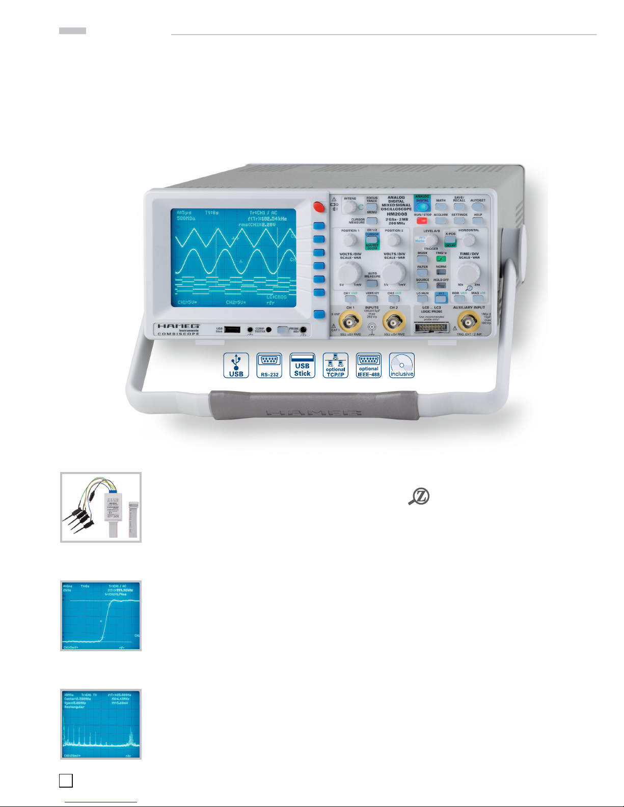
 2GSa/s Real Time Sampling, 20GSa/s Random Sampling

 2MPts Memory per Channel, Memory oom up to 100,000:1

 FFT for spectral analysis

 2 Channels + 4 Logic Channels with Option HO2010 (MSO)

 Deflection coefficients 1mV/div.…5V/div.,

with adjustable DC offset voltage;
Time Base 2ns/div.…50s/div.

 Acquisition modes: Single, Refresh, Average, Envelope,

Roll, Peak-Detect

 Front USB-Stick Connector for Screenshots

 USB/RS-232, optional: IEEE-488 or Ethernet/USB

 Signal display: Yt, XY and FFT;

Interpolation: Sinx/x, Pulse, Dot Join (linear)

 Adjustable input impedance 1MΩ/50Ω

 See HM2005-2 for analog mode

200MHz Mixed Signal

CombiScope

®

HM2008

HM2008

Frequency Analysis of a
Video Signal with FFT

Rise Time Measurement
in DSO Mode with 2ns/div.,
2GSa/s

Logic Probe HO2010

5

Subject to change without notice

Specifications

200 MHz Mixed Signal CombiScope®HM2008

All data valid at 23 °C after 30 minute warm-up

Vertical Deflection

Channels:

Analog: 2
Digital: 2 + (additionally with Option HO2010) 4 Logic

Channels

Operating Modes:

Analog: CH 1 or CH 2 separate, DUAL (CH 1 and

CH 2 alternate or chopped), Addition

Digital: Analog Signal Channels: CH 1 or CH 2

separate, DUAL (CH 1 and CH 2) or Addition.
Logic Signal Channels (LCH 0…3) switchable.

X in XY-Mode: CH 1
Invert: CH 1, CH 2
Bandwidth (-3dB): 2 x 0…200 MHz
Rise time: ‹ 1,75 ns
Bandwidth Limiter (switchable): approx. 20MHz (1 mV/div.…5V/div.)
Deflection Coefficients (CH 1, 2): 12 calibrated steps

1…2 mV/div.: ± 3 % (0…100MHz (-3 dB))
5 mV…5 V/div.: ± 3 % (1-2-5 sequence)
variable (uncalibrated): › 1 mV/div.…5V/div., continuous

Inputs CH 1, 2:

Impedance: 1 MΩ II 13 pF
Coupling: DC, AC, 50Ω, GND (ground)
Offset control:

1 mV, 2 mV ± 0.2 V
5…50mV ±1V
100mV…5V ±20V

Max. Input Voltage: 250 V (DC + peak AC), 50Ω ‹ 5V

rms

Y Delay Line (analog): 70 ns
Measuring Circuits: Measuring Category I
Analog mode only:

Auxiliary input:
Function (selectable): Ext. Trigger, Z (unblank in analog mode)
Coupling (Ext. Trig./ Z): all/AC, DC

Max. input voltage: 100 V (DC + peak AC)
Digital mode only:
Logic Channels in combination with Option HO2010:

Quantity 4 (LCH 0…3)
Select. switching thresholds: TTL, CMOS, ECL (common for all)
User definable thresholds: 2

within the range: -2…+8 V (common for all)

Triggering

Analog and Digital Mode
Automatic (Peak to Peak):

Min. signal height: 5mm

Frequency range: 10Hz…250 MHz

Level control range: from Peak- to Peak+
Normal (without peak):

Min. signal height: 5mm

Frequency range: 0…250MHz

Level control range: –10…+10 div.
Operating modes: Slope/Video/Logic
Slope: Rising, falling, both
Sources: CH 1, CH 2, alt. CH 1/2 (≥ 8 mm, analog

mode only), Line, Ext.

Coupling: AC: 10 Hz…250MHz

DC: 0…250 MHz
HF: 30 kHz…250MHz
LF: 0…5 kHz

Noise Rej. switchable

Video: pos. /neg. Sync. Impulse

Standards: 525 Line/60 Hz Systems

625 Line/50 Hz Systems

Field: even/odd/both

Line: all/line number selectable

Source: CH 1, CH 2, Ext.
Indicator for trigger action: LED
External Trigger via: AUXILIARY INPUT (0.3 Vpp, 0…200MHz)
Coupling: AC, DC
Max. input voltage: 100V (DC + peak AC)
Digital mode:
Pre/Post Trigger: -100…+400 % relative to complete memory

Analog mode:
2nd Trigger

Min. signal height: 5mm

Frequency range: 0…250MHz

Coupling: DC

Level control range: -10…+10 div.

Horizontal Deflection

Analog Time Base

Operating modes: A, ALT (alternating A/B), B

Time base A: 20 ns/ div.…0.5 s/ div. (1-2-5 sequence)

Time base B: 20 ns/div…20 ms/div. (1-2-5 sequence)

Accuracy A and B: ±3%

X Magnification x10: to 2 ns/div.

Accuracy: ±5%
Variable time base A/B: cont. 1:2.5
Hold Off time: var. 1:10 (LED-Indication)

Analog XY Mode
Bandwidth X-Amplifier: 0…3 MHz (-3dB)
X Y phase shift: ‹ 3° ‹ 220kHz
Digital Time Base
Time base range (1-2-5 sequence)

Refresh Mode: 2 ns/div.…50s/div.
with Peak Detect: 500ns/div.…50 s/div. (min. Pulse Width 10 ns)
Roll Mode: 50 ms/div.…50s/div.

Accuracy time base

Time coefficient: 50 ppm
Display: ±1%

MEMORY ZOOM: max. 100,000:1
Digital XY Mode

Bandwidth X-Amplifier: 0…200 MHz (-3dB)
XY phase shift: ‹ 3° ‹ 200 MHz

Digital Storage

Sampling Rate (real time): Analog channels: 2 x 1 GSa/s or 1 x 2GSa/s

(interleaved);
Logic Channels: max. 4 x 500 MSa/s

Sampling Rate (random sampling): 20 GSa/s (1-Channel mode)

25 GSa/s (2-Channel mode)

Bandwidth: 2 x 0…200 MHz (Random)
Memory: 2 x 2MPts (analog); 4 x 2 MPts (logic)
Operating modes: Refresh, Average, Envelope, Roll:

Free Run/ Triggered, Peak-Detect

Resolution (vertical): 8Bit (25 Pts/ div.)
Resolution (horizontal):

Yt: 11Bit (200 Pts/ div.)
XY: 8Bit (25 Pts/div.)

Interpolation: Sinx/ x, Dot Join (linear)
Delay: 2 Million x (1/Sampling Rate; max.)

8 Million x (1/Sampling Rate; max.)

Display refresh rate: max.170/s at 2 MPts
Display: Dots (acquired points only), Vectors (inter-

polation), Optimal (complete memory
weighting and vector display)

Reference Memories: 9 with 2 kPts each (for recorded signals)
Display: 2 signals of 9 (freely selectable)

FFT Mode

Display X: Frequency Range
Display Y: True rms value of spectrum

Scaling: Linear or logarithmic
Level display: dBV, V

Window: Square, Hanning, Hamming, Blackman
Control: Center frequency, Span
Marker: Frequency, Amplitude
Zoom (frequency axis): up to x20

Operation/Measuring /Interfaces

Operation: Menu (multilingual), Autoset, Help functions (multilingual)
Save/Recall internal:

analog: 9 Instrument parameter settings
digital: 9 Signals (each 2k) incl. instrument parameters
Signal sources: CH 1, CH 2, LCH 0…3, ZOOM, Reference 1–9

or Mathematics

Signal display: max. 6 signals

USB Memory-Stick:

Save/Recall external:
Instrument settings and Signals: CH1, CH2, LCH 0…3, ZOOM,

Reference 1–9 or Mathematics

Screen-shot: as Bitmap
Signal display data (2k per channel): Binary (SCPI-Data), Text (ASCII-

Format), CSV (Spread Sheet)

Logic (with Option HO2010): AND/OR, TRUE/FALSE

Source: Logic Channel 0…3
State: X, H, L

6

Subject to change without notice

Important hints

Frequency counter:

6 digit resolution: › 1…250MHz
5 digit resolution: 0.5 Hz…1MHz
Accuracy: 50 ppm

Auto Measurements:

Analog mode: Frequency, Period, V

dc

, Vpp, Vp+, V

p-

plus in digital mode: V

rms

, V

avg

Cursor Measurements:

Analog mode: Δt, 1/Δt (f), tr, ΔV, V to GND, ratio X, ratio Y
plus in digital mode: V

pp

, Vp+, Vp-, V

avg

, V

rms

, pulse count

Resolution Readout/Cursor: 1000 x 2000 Pts, Signals: 250 x 2000
Interfaces (plug-in): USB/RS-232 (HO720)
Optional: IEEE-488, Ethernet/USB

Mathematic functions

Number of Formula Sets: 5 with 5 formulas each
Sources: CH 1, CH 2, Math 1 - Math 5
Targets: 5 math. memories (Math 1…5)
Functions: ADD, SUB, 1/X, ABS, MUL, DIV, SQ, POS,

NEG, INV

Display: max. 2 math. memories (Math 1…5)

Display

CRT: D14-375GH
Display area (with graticule): 8div. x 10 div.
Acceleration voltage: approx. 14 kV

General Information

Component tester

Test voltage: approx. 7V

rms

(open circuit), approx. 50Hz

Test current: max. 7mA

rms

(short circuit)

Reference Potential: Ground (safety earth)

Probe ADJ Output: 1 kHz/ 1MHz square wave signal 0.2 V

pp

(tr ‹ 4 ns)

Trace rotation: electronic
Line voltage: 105…253V, 50/60 Hz ±10 %, CAT II
Power consumption: 48 Watt at 230 V, 50 Hz
Protective system: Safety class I (EN61010-1)
Operating temperature: +5…+40°C
Storage temperature: -20…+70 °C
Rel. humidity: 5…80% (non condensing)
Dimensions (W x H x D): 285 x 125 x 380 mm
Weight: 5.6kg

Important hints

Please check the instrument for mechanical damage or loose
parts immediately after unpacking. In case of damage we advise
to contact the sender. Do not operate.

List of symbols used:

Consult the manual High voltage

Important note Ground

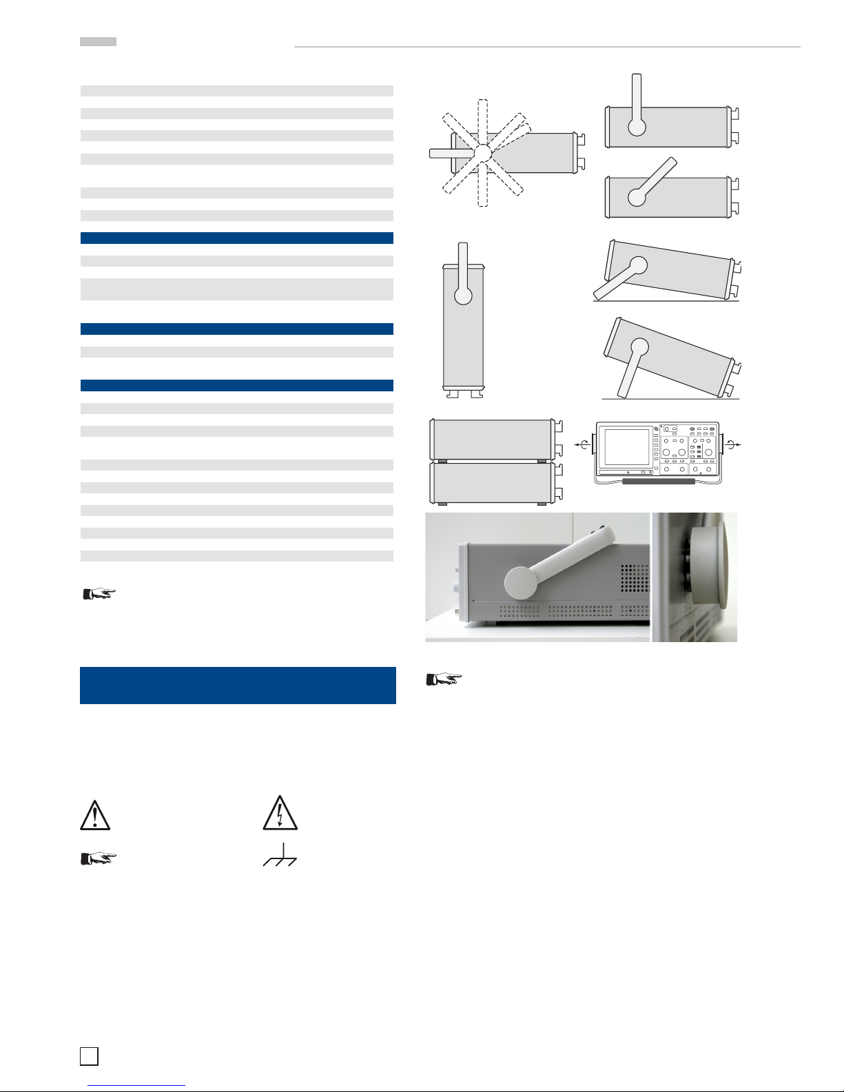
Positioning the instrument

As can be seen from the fi gures, the handle can be set into
different positions:
A and B = carrying
C = horizontal operating
D and E = operating at different angles
F = handle removal
T = shipping (handle unlocked)

A

A

B

B

C

C

D

D

E

E

T

F

PUkT

PUkT

PUk PUk

PUk PUk

PUk PUk

PUkT PUkT

PUkT

PUkT

PUkT

HGOPFFD

PUkT
HGOFFD

PUOPFGkT

PUkT

PUkTKl

15pF
max

400 Vp

PUOPFGkT

PUOPFGkT

PUOPFGkT

PUOPFGkT

PGkT

PUOPFGkT

PUOPFGkT

PFGkT

PUOPFGkT PUOPFGkT

PUOPFGkT

PUOPFGkT

PUOPFGkT

HAMEG

PUOPFGkT

PUOPFGkT

PUOPFGkT

ANALOG
DIGITAL

MIXED SIGNAL

COMBISCOPE

HM1508

1 GSa · 1MB

150 MHz

PUOGkT

VOLTS/DIVV
HGOPFFD

VOLTS/DIVV
HGOPFFD

VOLTS/DIVV
HGOPFFD

PUkT
HGOPFFD

PUkT
HGOPFFD

PUkT

PUkT

PUkT

PUkT

PUkT

PUkT

PUkT

PUkTKl

15pF
max
400 Vp

PUOPFGkT
INPUTS

PUOPF

PUOPF

PUOPF

PUOPF PUOPF

C O M B I S C O P E

B

T

T

Attention!

When changing the handle position, the instrument

must be placed so that it can not fall (e.g. placed
on a table). Then the handle locking knobs must be
simultaneously pulled outwards and rotated to the
required position. Without pulling the locking knobs
they will latch in into the next locking position.

Handle mounting/dismounting

The handle can be removed by pulling it out further, depending
on the instrument model in position B or F.

Safety

The instrument fulfi ls the VDE 0411 part 1 regulations for
electrical measuring, control and laboratory instruments and
was manufactured and tested accordingly. It left the factory in
perfect safe condition. Hence it also corresponds to European
Standard EN 61010-1 resp. International Standard IEC 1010-1.
In order to maintain this condition and to ensure safe operation
the user is required to observe the warnings and other directions
for use in this manual. Housing, chassis as well as all measu­ring terminals are connected to safety ground of the mains.
All accessible metal parts were tested against the mains with
2200 V

DC

. The instrument conforms to safety class I.

For Accessories supplied and options please refer

to page 24.

7

Subject to change without notice

Important hints

Type of fuse:

Size 5 x 20 mm; 250V~, C;
IEC 127, Bl. III; DIN 41 662
(or DIN 41 571, Bl. 3).
Cut off: slow blow (T) 0,8A.

The oscilloscope may only be operated from mains outlets with
a safety ground connector. The plug has to be installed prior to
connecting any signals. It is prohibited to separate the safety
ground connection.
Most electron tubes generate X-rays; the ion dose rate of this in­strument remains well below the 36 pA/kg permitted by law.
In case safe operation may not be guaranteed do not use the
instrument any more and lock it away in a secure place.

Safe operation may be endangered if any of the following
was noticed:

– in case of visible damage.
– in case loose parts were noticed
– if it does not function any more.
– after prolonged storage under unfavourable conditions (e.g.

like in the open or in moist atmosphere).

– after any improper transport (e.g. insuffi cient packing not

conforming to the minimum standards of post, rail or trans­port fi rm)

Proper operation

Please note: This instrument is only destined for use by person­nel well instructed and familiar with the dangers of electrical
measurements. For safety reasons the oscilloscope may only
be operated from mains outlets with safety ground connector.
It is prohibited to separate the safety ground connection. The
plug must be inserted prior to connecting any signals.

CAT I

This oscilloscope is destined for measurements in circuits not
connected to the mains or only indirectly. Direct measurements,
i.e. with a galvanic connection to circuits corresponding to the
categories II, III, or IV are prohibited!
The measuring circuits are considered not connected to the
mains if a suitable isolation transformer fulfi lling safety class
II is used. Measurements on the mains are also possible if
suitable probes like current probes are used which fulfi l the
safety class II. The measurement category of such probes must
be checked and observed.

Measurement categories

The measurement categories were derived corresponding to
the distance from the power station and the transients to be
expected hence. Transients are short, very fast voltage or cur­rent excursions which may be periodic or not.
Measurement CAT IV: Measurements close to the power station,
e.g. on electricity meters
Measurement CAT III: Measurements in the interior of buildings
(power distribution installations, mains outlets, motors which
are permanently installed).
Measurement CAT II: Measurements in circuits directly connec­ted to the mains (household appliances, power tools etc).
Measurement CAT I: Electronic instruments and circuits which
contain circuit breakers resp. fuses.

Environmental conditions

The oscilloscope is destined for operation in industrial, business,
manufacturing, and living sites.
Operating ambient temperature: +5 °C to +40 °C. During
transport or storage the temperature may be –20 °C to +70°C.
Please note that after exposure to such temperatures or in
case of condensation proper time must be allowed until the
instrument has reached the permissible temperature, resp.
until the condensation has evaporated before it may be turned
on! Ordinarily this will be the case after 2 hours. The oscillo­scope is destined for use in clean and dry environments. Do

not operate in dusty or chemically aggressive atmosphere or if
there is danger of explosion.
The operating position may be any, however, suffi cient ventila­tion must be ensured (convection cooling). Prolonged operation
requires the horizontal or inclined position.

Do not obstruct the ventilation holes!

Specifi cations are valid after a 30 minute warm-up period
between 15 and 30 degr. C. Specifi cations without tolerances
are average values.

Warranty and repair

HAMEG instruments are subjected to a strict quality control.
Prior to leaving the factory, each instrument is burnt-in for 10
hours. By intermittent operation during this period almost all
defects are detected. Following the burn-in, each instrument is
tested for function and quality, the specifi cations are checked
in all operating modes; the test gear is calibrated to national
standards.
The warranty standards applicable are those of the country
in which the instrument was sold. Reclamations should be
directed to the dealer.

Only valid in EU countries

In order to speed reclamations customers in EU countries may
also contact HAMEG directly. Also, after the warranty expired,
the HAMEG service will be at your disposal for any repairs.

Return material authorization (RMA):

Prior to returning an instrument to HAMEG ask for a RMA
number either by internet (http://www.hameg.com) or fax. If
you do not have an original shipping carton, you may obtain one
by calling the HAMEG service dept (++49 (0) 6182 800 500) or by
sending an email to [e-mail].

Maintenance

Clean the outer shell using a dust brush in regular intervals.
Dirt can be removed from housing, handle, all metal and plastic
parts using a cloth moistened with water and 1 % detergent.
Greasy dirt may be removed with benzene (petroleum ether) or
alcohol, there after wipe the surfaces with a dry cloth. Plastic
parts should be treated with an antistatic solution destined
for such parts. No fl uid may enter the instrument. Do not use
other cleansing agents as they may adversely affect the plastic
or lacquered surfaces.

Line voltage

The instrument has a wide range power supply from 105 to
253 V, 50 or 60 Hz ±10%. There is hence no line voltage selector.
The line fuse is accessible on the rear panel and part of the line
input connector. Prior to exchanging a fuse the line cord must be
pulled out. Exchange is only allowed if the fuse holder is undama­ged, it can be taken out using a screwdriver put into the slot. The
fuse can be pushed out of its holder and exchanged.
The holder with the new fuse can then be pushed back in place
against the spring. It is prohibited to ”repair“ blown fuses or to
bridge the fuse. Any damages incurred by such measures will
void the warranty.

8

Subject to change without notice

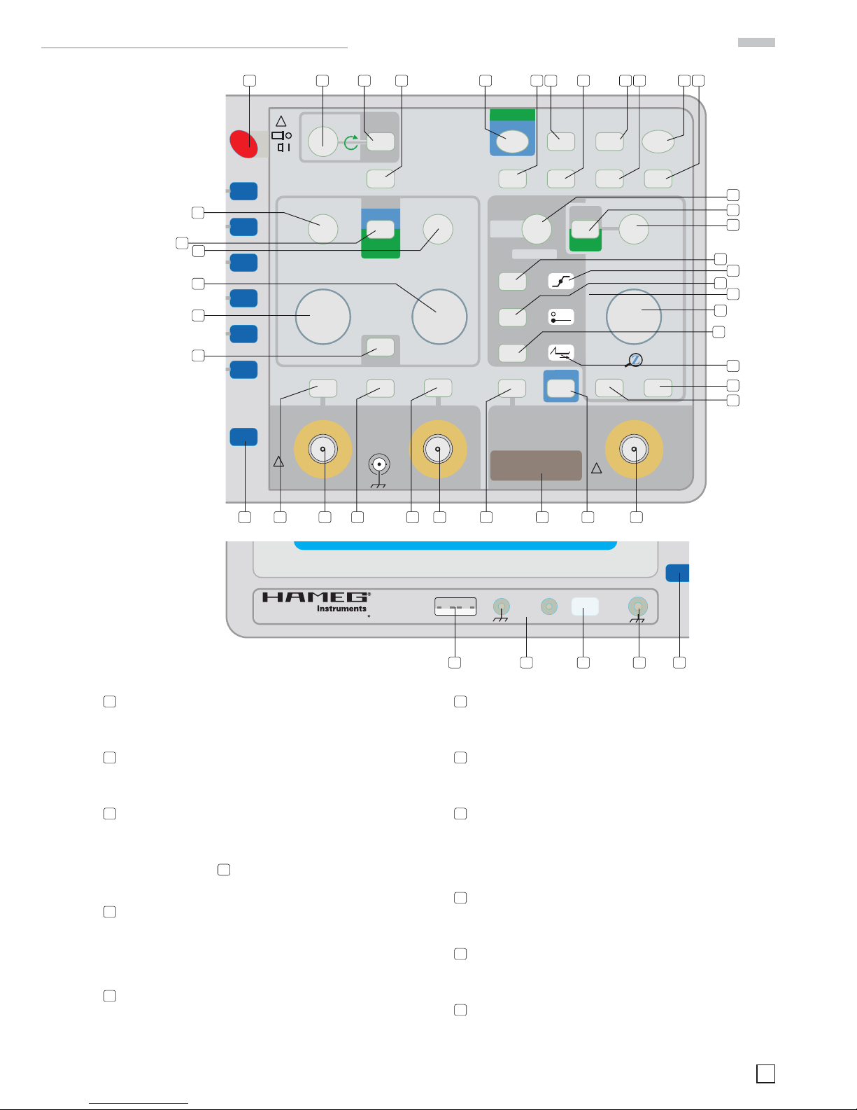
Front Panel Elements – Brief Description

Front Panel Elements – Brief Description

1

POWER (pushbutton) 26

Turns scope on and off.

2

INTENS (knob) 26

Intensity for trace- and readout brightness, focus and trace

rotation control.

3

FOCUS, TRACE, MENU (pushbutton) 26

Calls the Intensity knob menu to be displayed and enables

the change of different settings using the INTENS knob. See
item 2.

4

CURSOR MEASURE (pushbutton) 26

Calls the CURSOR menu and offers measurement selection

and activation.

5

ANALOG/DIGITAL (pushbutton) 27

Switches between analog (green) and digital mode (blue).

6

RUN / STOP (pushbutton) 27
RUN: Signal data acquisition enabled.
STOP (constantly lit): Signal data acquisition is stopped
STOP (fl ashing): Signal data acquisition is in progress and

will be stopped after being completed.

7

MATH (pushbutton) 28
Calls mathematical function menu if digital mode is present.

8

ACQUIRE (pushbutton) 29
Calls the signal capture and display mode menu in digital

mode.

9

SAVE/RECALL (pushbutton) 30
Offers access to the reference signal (digital mode only) and

the instrument settings memory.

10

SETTINGS (pushbutton) 31
Opens menu for language and miscellaneous function; in

digital mode also signal display mode.

11

AUTOSET (pushbutton) 32
Enables appropriate, signal related, automatic instrument

settings.

12

HELP (pushbutton) 32
Switches help texts regarding controls and menus on/off.

13

POSITION 1 (knob) 32
Controls position of actual present functions

15

: Signal
(current, reference or mathematics), Cursor and ZOOM
(digital).

14

POSITION 2 (knob) 33

Controls position of actual present functions

15

: Signal
(current, reference or mathematics) Cursor and ZOOM
(digital).

15

CH1/2-CURSOR-MA/REF-ZOOM (pushbutton) 34

Calls the menu and indicates the current function of POSI-

TION 1 and 2 controls.

16

VOLTS/DIV-SCALE-VAR (knob) 34

Channel 1 Y defl ection coeffi cient, Y variabel and Y scaling
setting.

17

VOLTS/DIV-SCALE-VAR (knob) 34

Channel 2 Y defl ection coeffi cient, Y variabel and Y scaling

setting.

18

AUTO MEASURE (pushbutton) 35

Calls menus and submenus for automatic measurement.

19

LEVEL A/B – FFT-Marker (knob) 36

Trigger level control for A- and B Time Base. Marker position

shift in FFT mode.

20

MODE (pushbutton) 36

Calls selectable trigger modes.

21

FILTER (pushbutton) 37

Calls menu for trigger fi lter (coupling), noise reject and slope

selection.

22

SOURCE (pushbutton) 38

Calls trigger source menu (e.g. CH1, CH2, Alt. 1/2, External,

AC Line).

23

TRIG’d (LED) 38

Lit when the trigger signal meets the trigger conditions.

24

NORM (LED) 38

Lit if normal or single event triggering is chosen.

25

HOLD OFF (LED) 38

Lit if a hold off time is set (only in analog mode) > 0% in the

HOR menu (HOR VAR pushbutton

30

).

26

X-POS / DELAY (pushbutton) 38

Calls and indicates (colour) the actual function of the HO-

RIZONTAL knob

27

, (X-POS = dark).

27

HORIZONTAL (knob) 39

Changes the X position or in digital mode, the delay time

(Pre- or Post-Trigger).

In FFT mode for center frequency control.

28

TIME/DIV-SCALE-VAR (knob) 39

Setting of A and B time base (defl ection coeffi cient), time

fi ne control (VAR; only in analog mode) and scaling; Span
in FFT mode.

29

MAG x10 (pushbutton) 40

10 fold expansion in X direction in analog Yt mode, with

simultaneous change of the defl ection coeffi cient display
in the readout.

30

HOR / VAR (pushbutton) 41

Calls ZOOM function (digital); in analog mode time base A

and B, time base variable and hold off control.

31

CH1 / VAR (pushbutton) 42

Calls channel 1 menu with input coupling (AC, DC, 50 Ohm,

GND), inverting, probe, signal input offset and Y variable
control.

32

VERT/XY (pushbutton) 43

Calls vertical mode selection, addition, XY mode and band-

width limiter.

33

CH2 / VAR (pushbutton) 44

Calls channel 1 menu with input coupling (AC, DC, 50 Ohm,

GND), inverting, probe, signal input offset and Y variable
control.

The fi gures indicate the page for complete discription

in the chapter CONTROLS AND READOUT

▼

9

Subject to change without notice

Front Panel Elements – Brief Description

34

INPUT CH1 (BNC-socket) 45

Channel 1 signal input and input for horizontal defl ection in

XY mode.

35

INPUT CH2 (BNC-socket) 45

Channel 2 signal input and input for vertical deflection in XY

mode.

36

LC/AUX (pushbutton) 45

Digital mode: Logic signal channels LC0 to LC3 activa-

tion/deactivation and threshold setting. Analog mode: If
external triggering is not chosen, activation/deactivation of
AUXILIARY INPUT

38

for intensity modulation (Z) and input

coupling selection.

37

FFT (pushbutton) 46

Calls FFT menu, offers window and scaling selection, as

well as function switch off.

Calls FFT menu if FFT mode is present. Direct switch over

from digital Yt mode to FFT mode.

38

AUXILIARY INPUT (BNC socket) 46
Digital mode: Input for external trigger signals.
Analog mode: Input for intensity modulation (Z) or external

trigger signals.

39

LC0 ... LC3 LOGIC PROBE (multi pin connector) 47

Digital mode: In connection with Option HO2010 input for

logic signals.

40

PROBE / ADJ (socket) 47

Square wave signal output for frequency compensation of

x10 probes.

41

PROBE / ADJ (pushbutton) 47

Calls menu that offers COMPONENT Tester operation, fre-

quency selection of PROBE ADJ square wave signal, hard­ware and software information and details about interface
(rear side) and USB Stick (fl ash drive) connector.

42

COMPONENT TESTER (2 sockets with 4 mm Ø) 47

Connectors for test leads of the Component Tester. Left

socket is galvanically connected with protective earth.

43

USB Stick (USB fl ash drive connector; front side) 47

Enables storage and load of signals and signal parameters

in connection with USB fl ash drives.

44

MENU OFF (pushbutton) 47

Switches the menu display off or one step back in the menu

hierarchy.

FFT­Marker

VAR VAR VA R x10

VOLTS / DIV

SCALE · VAR

VOLTS / DIV

SCALE · VAR

TIME / DIV

SCALE · VAR

AUTO

MEASURE

5 V 1 mV 5 V 1 mV

X-POS

AUXILIARY INPUTLC0 ... LC

3

LOGIC PROBE

Use recommended

probe only!

TRIG. EXT. / Z-INP.

INTENS

!

LEVEL A/B

HM2008

2 GSa · 2 MB

200 MHz

50s 2ns

LC/AUX

FFT

1MΩ II

15pF

max

100 Vp

HORIZONTAL

INPUTS

1MΩII15pF

max

250 Vp

DIGITAL

ANALOG

DELAY

CH 1/2

CURSOR

X-INP

FOCUS
TRACE

MENU

CURSOR

MEASURE

MA/REF

ZOOM

MATH

SAVE/

RECALL

AUTOS ET

RUN / STOP ACQUIRE SETTINGS HELP

MODE

FILTER

SOURCE

TRIG ’d

NORM

HOLD OFF

TRIGGER

POSITION 1 POSITION 2

CH 1

VERT/XY

CH 2 HOR MAG

CAT I

!

50Ω ≤5V RMS 50Ω ≤5V RMS

CH 1 CH 2

!

ANALOG

DIGITAL

MIXED SIGNAL

OSCILLOSCOPE

POWER

POWER

MENU

MENU

OFF

OFF

1 2 3 4 5 76

10

8

12911

19

26

27

23

24

25

29

30

38

22

20

21

28

373936353332343144

13

15

14

17

16

18

COMBISCOPE

USB

Stick

COMP.

TESTER

PROBE

ADJ

POWER

MENUMENU

OFFOFF

4440414243

10

Subject to change without notice

Basic signal measurement

Signals which can be measured

The following description pertains to analog and digital ope­ration. The different specifications in both operating modes
should be kept in mind.

The oscilloscope HM2008 can display all repetitive signals
with a fundamental repetition frequency of at least 200 MHz.
The frequency response is 0 to 200 MHz (–3 dB). The vertical
amplifi ers will not distort signals by overshoots, undershoots,
ringing etc.

Simple electrical signals like sine waves from line frequency
ripple to hf will be displayed without problems. However, when
measuring sine waves, the amplitudes will be displayed with
an error increasing with frequency. At 120 MHz the amplitude
error will be around –10 %. As the bandwidths of individual
instruments will show a certain spread (the 200 MHz are a
guaranteed minimum) the actual measurement error for sine
waves cannot be exactly determined.

Pulse signals contain harmonics of their fundamental fre­quency which must be represented, so the maximum useful
repetition frequency of nonsinusoidal signals is much lower
than 200 MHz (5 to 10 times). The criterion is the relationship
between the rise times of the signal and the scope; the scope’s
rise time should be <1/3 of the signal’s rise time if a faithful
reproduction without too much rounding of the signal shape
is to be preserved.

The display of a mixture of signals is especially diffi cult if it con­tains no single frequency with a higher amplitude than those of
the other ones as the scope’s trigger system normally reacts to
a certain amplitude. This is e.g. typical of burst signals. Display
of such signals may require using the HOLD-OFF control.

Composite video signals may be displayed easily as the instru­ment has a TV SYNC separator.

The maximum sweep speed of 2 ns/cm allows suffi cient time
resolution, e.g. a 200 MHz sine wave will be displayed one
period per 2.5 cm. The vertical amplifi er inputs may be DC or
AC coupled. Use DC coupling only if necessary and preferably
with a probe.

Low frequency signals when AC coupled will show tilt (AC low
frequency – 3 dB point is 1.6 Hz), so if possible use DC coupling.
Using a probe with 10:1 or higher attenuation will lower the
–3 dB point by the probe factor. If a probe cannot be used due
to the loss of sensitivity DC coupling the scope and an external
large capacitor may help which, of course, must have a suffi cient
DC rating. Care must be taken, however, when charging and
discharging a large capacitor.

DC coupling is preferable with all signals of varying duty cycle,
otherwise the display will move up and down depending on the
duty cycle. Of course, pure DC can only be measured with DC
coupling.
The readout will show which coupling was chosen: = stands
for DC, ~ stands for AC. For hf measurement an internal 50 Ω
terminator can be activated which is indicated by an Ω-symbol
in the readout.

Amplitude of signals

In contrast to the general use of rms values in electrical engi­neering oscilloscopes are calibrated in Vpp as that is what is
displayed.

Derive rms from V

pp

: divide by 2.84. Derive Vpp from rms: mul-

tiply by 2.84.

Values of a sine wave signal

V

rms

= rms value

V

pp

= pp – value

V

mom

= momentary value, depends on time vs. period.

The minimum signal for a one cm display is 1 mV

pp

±5 % provi­ded 1 mV/cm was selected and the variable is in the calibrated
position.

The available sensitivities are given in mV

pp

or Vpp. The cursors
allow to indicate the amplitudes of the signals immediately on
the readout as the attenuation of probes is automatically taken
into account. Even if the probe attenuation was selected manu­ally this will be overridden if the scope identifi es a probe with
an identifi cation contact as different. The readout will always
give the true amplitude.

It is important that the variable be in its calibrated position. The
sensitivity may be continuously decreased by using the variable
(see Controls and Readout). Each intermediate value between
the calibrated positions 1–2–5 may be selected. Without using
a probe thus a maximum of 100 V

PP

may be displayed (20 V/div

x 8 cm screen x 2.5 variable).

Amplitudes may be directly read off the screen by measuring
the height and multiplying by the V/div. setting.

Please note: Without a probe the maximum permis-

sible voltage at the inputs must not exceed 250 Vp
irrespective of polarity.

In case of signals with a DC content the peak value DC + AC
peak must not exceed + or –250 V

p

. Pure AC of up to 500 Vpp is

permissible.

If probes are used their possibly higher ratings are

only usable if the scope is DC coupled.

In case of measuring DC with a probe while the scope input is
AC coupled the capacitor in the scope input will see the input
DC voltage as it is in series with the internal 1 MΩ resistor.
This means that the maximum DC voltage (or DC + peak AC) is
that of the scope input, i.e. 250 V

P

! With signals which contain
DC and AC the DC content will stress the input capacitor while
the AC content will be divided depending on the AC impedance

Basic signal measurement

V

p

V

rms

V

mom

V

pp

11

Subject to change without notice

of the capacitor. It may be assumed that this is negligible for
frequencies >40 Hz.

Considering the foregoing you may measure DC signals of up to
600 V or pure AC signals of up to 1200 V

PP

with a HZ200 probe.
Probes with higher attenuation like HZ53 100:1 allow to measure
DC up to 1200 V and pure AC of up to 2400 V

PP

. (Please note
the derating for higher frequencies, consult the HZ53 manual).
Stressing a 10:1 probe beyond its ratings will risk destruction of
the capacitor bridging the input resistor with possible ensuing
damage of the scope input!

In case the residual ripple of a high voltage is to be measured a
high voltage capacitor may be inserted in front of a 10:1 probe, it
will take most of the voltage as the value of the probe’s internal
capacitor is very low, 22 to 68 nF will be suffi cient.

If the input selector is switched to Ground the reference trace
on the screen may be positioned at graticule center or else­where.

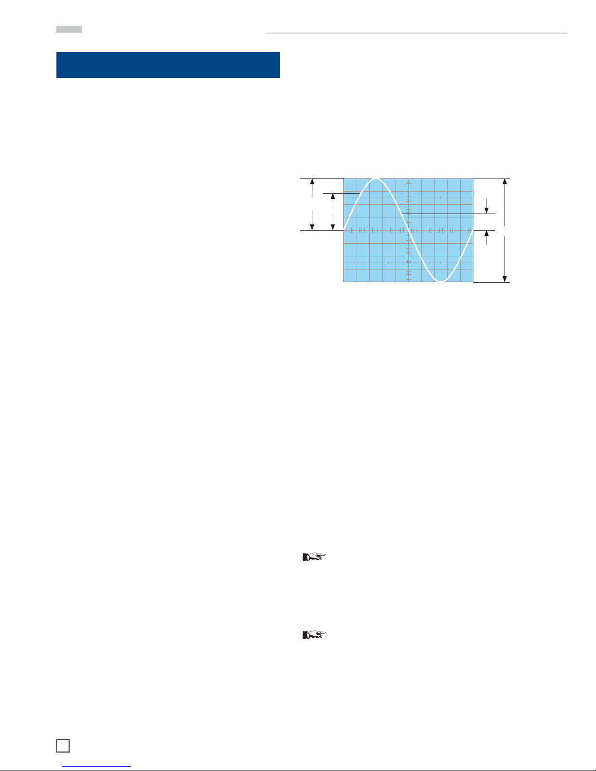
DC and AC components of an input signal

The dashed curve shows an AC signal symmetrical to zero. If
there is a DC component the peak value will be DC + AC peak.

Timing relationships

In most cases repetitive signals must be measured. The repe­tition frequency of a signal is equal to the number of periods
per second. Depending on the TIME/DIV setting one or more
periods or part of a period of the signal may be displayed. The
time base settings will be indicated on the readout in s/cm,
ms/cm, μs/cm and ns/cm (1 cm is the equivalent of 1 div. on
the crt graticule). Also the cursors may be used to measure the
frequency or the period.

Without cursor the cycle duration can be determined by multi­plying the length (cm) with the (calibrated) time coeffi cient. The
reciprocal value is the frequency.

If portions of the signal are to be measured use delayed sweep
(analog mode) or zoom (digital mode) or the magnifi er x 10. Use
the HORIZONTAL positioning control to shift the portion to be
zoomed into the screen center.

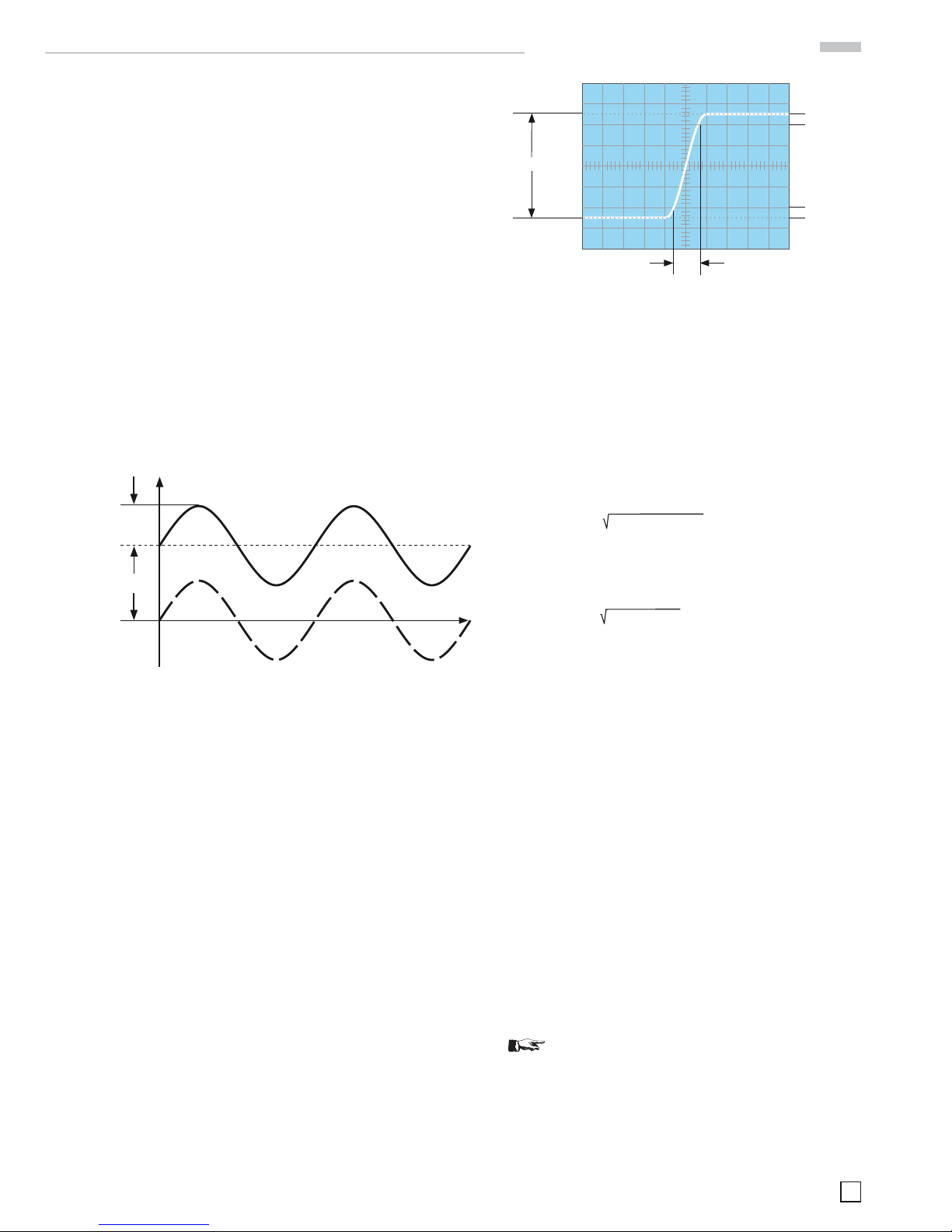
Pulse signals are characterized by their rise and fall times
which are measured between the 10 % and 90 % portions. The
following example uses the internal graticule of the crt, but also
the cursors may be used for measurement.

Measurement:

– Adjust the rising portion of the signal to 5 cm.

– Position the rising portion symmetrically to the graticule

centre line, using both Y and X positioning controls.

– Notice the intersections of the signal with the 10 and 90 %

lines and project these points to the centre line in order to
read the time difference.

In the example it was 1.6 cm at 5 ns/cm equals 8 ns rise time.

When measuring very short rise times coming close to the scope
rise time it is necessary to subtract the scope’s (and if used the
probe’s) rise times geometrically from the rise time as seen on
the screen. The true signal rise time will become:

t

tot

is the rise time seen, t

osc

is the scope’s own rise time (1.75

ns with the HM2008), t

t

is the rise time of the probe, e.g. 2 ns.
If the signal’s rise time is >22 ns, the rise times of scope and
probe may be neglected.

For the measurement of rise times it is not necessary to proceed
as outlined above. Rise times may be measured anywhere on
the screen. It is mandatory that the rising portion of the signal
be measured in full and that the 10 to 90 % are observed. In
case of signals with over- or undershoot the 0 and 100 % levels
are those of the horizontal portions of the signal, i.e. the over­resp. undershoots must be disregarded for rise and fall time
measurements. Also, glitches will be disregarded. If signals
are very distorted, however, rise and fall time measurements
may be of no value.

For most amplifi ers, even if their pulse behaviour is far from
ideal, the following relationship holds:

350 350
t

a

=

——

B =

——

B t

a

tr/ns = 350/Bandwidth/MHz

Connection of signals

In most cases pressing the AUTOSET button will yield a satisf­actory display (see AUTOSET). The following relates to special
cases where manual settings will be advisable. For a description
of controls refer to ”Controls and Readout“.

Take care when connecting unknown signals to the

inputs!

It is recommended to use probes whenever possible. Without
a probe start with the attenuator set to its 20 V/cm position.
If the trace disappears the signal amplitude may be too large
overdriving the vertical amplifi er or/and its DC content may be
too high. Reduce the sensitivity until the trace will reappear

Basic signal measurement

ta= 82 - 2.32 - 22 = 7,5 ns

ta= t

tot

2

– t

osc

2

– t

t

2

voltage

peak

AC

DC

DC

AC

DC + AC

peak

= 400 V

max

5 cm

t

tot

100%

90%

10%

0%

12

Subject to change without notice

onscreen. If calibrated measurements are desired it will be
necessary to use a probe if the signal becomes >40 V

pp

. Check
the probe specifi cations in order to avoid overstressing. If the
time base is set too fast the trace may become invisible, then
reduce the time base speed.

If no probe is used at least screened cable should be used,
such as HZ32 or HZ34. However, this is only advisable for low
impedance sources or low frequencies (<50 kHz). With high
frequencies impedance matching will be necessary.

Non sinusoidal signals particularly require impedance matching,
preferably at both ends. At the scope input, a 50 Ω termination is
selectable with a maximum load of 0.5 Watt (5 V

rms

, or in case of

sine wave signals, 14.7 V

pp

). If proper terminations are not used,
sizeable pulse aberrations will result. Also sine wave signals
of >100 kHz should be properly terminated. Most generators
control signal amplitudes only if correctly terminated.
For higher loads (up to 1 Watt; 7 V

rms

or 20 Vpp) HAMEG offers

the external 50 Ω termination HZ22.

For probes terminations are neither required nor allowed, they
would ruin the signal.

Probes feature very low loads at fairly low frequencies: 10 MΩ
in parallel to a few pF, valid up to several hundred kHz. How­ever, the input impedance diminishes with rising frequency to
quite low values. This has to be borne in mind as probes are,
e.g., entirely unsuitable to measure signals across high impe­dance high frequency circuits such as bandfi lters etc.! Here
only FET probes can be used. Use of a probe as a rule will also
protect the scope input due to the high probe series resistance
(9 MΩ). As probes cannot be calibrated exactly enough during
manufacturing individual calibration with the scope input used
is mandatory! (See Probe Calibration).

Passive probes will, as a rule, decrease the scope bandwidth
resp. increase the rise time. We recommend to use HZ200 pro­bes in order to make maximum use of the combined bandwidth.
HZ200 features 2 additional hf compensation adjustments.

Whenever the DC content is > 250 V

DC

coupling must be used in
order to prevent overstressing the scope input capacitor. This is
especially important if a 100:1 probe is used as this is specifi ed
for 1200 V

DC

+ peak AC.

AC coupling of low frequency signals may produce tilt.

If the DC content of a signal must be blocked it is possible to
insert a capacitor of proper size and voltage rating in front of the
probe, a typical application would be a ripple measurement.

When measuring small voltages the selection of the ground
connection is of vital importance. It should be as close to voltage
take-off point as possible, otherwise ground currents may de­teriorate the measurement. The ground connections of probes
are especially critical, they should be as short as possible and
of large size.

If a probe is to be connected to a BNC connector use

a probe tip to BNC adapter.

If ripple or other interference is visible, especially at high sen­sitivity, one possible reason may be multiple grounding. The
scope itself and most other equipment are connected to safety
ground, so ground loops may exist. Also, most instruments will
have capacitors between line and safety ground installed which
conduct current from the live wire into the safety ground.

First time operation and initial adjustments

Prior to fi rst time operation the connection between the instru­ment and safety ground must be ensured, hence the plug must
be inserted fi rst.

Use the red pushbutton POWER to turn the scope on. Several
displays will light up. The scope will then assume the set-up,
which was selected before it was turned off. If no trace and
no readout are visible after approximately 20 sec, push the
AUTOSET button.

As soon as the trace becomes visible select an average inten­sity with INTENS, then select FOCUS and adjust it, then select
TRACE ROTATION and adjust for a horizontal trace.

With respect to crt life use only as much intensity as necessary
and convenient under given ambient light conditions, if unused
turn the intensity fully off rather than turning the scope off and
on too much, this is detrimental to the life of the crt heater.
Do not allow a stationary point to stay, it might burn the crt
phosphor.

With unknown signals start with the lowest sensitivity 5 V/cm,
connect the input cables to the scope and then to the measu­ring object which should be deenergized in the beginning. Then
turn the measuring object on. If the trace disappears, push
AUTOSET.

Trace rotation TR

The crt has an internal graticule. In order to adjust the defl ected
beam with respect to this graticule the Trace Rotation control
is provided. Select the function Trace Rotation and adjust for a
trace which is exactly parallel to the graticule.

Probe adjustment and use

In order to ensure proper matching of the probe used to the
scope input impedance the scope contains a calibrator with
short rise time and an amplitude of 0.2 Vpp ± 1 %, equivalent
to 4 cm at 5 mV/cm when using 10:1 probes.

The inner diameter of the calibrator connector is 4.9 mm and
standardized for series F probes. Using this special connec­tor is the only way to connect a probe to a fast signal source
minimizing signal and ground lead lengths and to ensure true
displays of pulse signals.

1 kHz – adjustment

This basic adjustment will ensure that the capacitive at­tenuation equals the resistive attenuation thus rendering the
attenuation of the probe independent of frequency. 1:1 probes
can not be adjusted and need no such adjustment anyway.

First time operation and initial adjustments

incorrect correct incorrect

13

Subject to change without notice

Operating modes of the vertical amplifi er

The controls most important for the vertical amplifi er are: VERT/
XY

32

, CH 1 31, CH 2 33 – and in digital mode also – LC/AUX 36.
They give access to the menus containing the operating modes
and the parameters of the individual channels.

Changing the operating mode is described in the chapter:
”Controls and Readout“.

Remark: Any reference to ”both channels“ always refers to
channels 1 and 2.

Usually oscilloscopes are used in the Yt mode. In analog mode
the amplitude of the measuring signal will defl ect the trace
vertically while a time base will defl ect it from left to right.

The vertical amplifi ers offer these modes:
– One signal only with CH1.
– One signal only with CH2.

− Two signals with channels 1 and 2 (DUAL trace mode).

− Two signals displayed as one in addition (ADD) mode.

In digital mode the Option HO2010 additionally enables the logic
state display of 4 logic channels (LC0 ... LC3).

In DUAL mode both channels are operative. In analog mode
the method of signal display is governed by the time base (see
also ”Controls and Readout“). Channel switching may either
take place after each sweep (alternate) or during sweeps with
a high frequency (chopped).

The normal choice is alternate, however, at slow time base set­tings the channel switching will become visible and disturbing,
when this occurs select the chopped mode in order to achieve
a stable quiet display.

In digital mode no channel switching is necessary as each input
has its own A/D converter, signal acquisition is simultaneous.

In ADD mode the two channels 1 and 2 are algebraically ad­ded (±CH1 ±CH2). With + polarity the channel is normal, with
– polarity inverted. If + Ch1 and – CH2 are selected the difference
will be displayed or vice versa.

Same polarity input signals:

Both channels not inverted: = sum
Both channels inverted: = sum
Only one channel inverted: = difference

Opposite polarity input signals:

Both channels not inverted: = difference
Both channels inverted: = difference
One channel inverted: = sum.

Please note that in ADD mode both position controls will be
operative. The INVERT function will not affect positioning.

Often the difference of two signals is to be measured at signal
take-offs which are both at a high common mode potential.
While this one typical application of the difference mode one
important precaution has to be borne in mind: The oscillosco­pe vertical amplifi ers are two separate amplifi ers and do not
constitute a true difference amplifi er with as well a high CM
rejection as a high permissible CM range! Therefore please
observe the following rule: Always look at the two signals in
the one channel only or the dual modes and make sure that

Prior to adjustment make sure that the trace rotation adjust­ment was performed.

Connect the 10:1 probe to the input. Use DC coupling. Set the
VOLTS/DIV knob for a signal display height of 4 cm and TIME/
DIV to 0.2 ms/cm, both calibrated. Insert the probe tip into the
calibrator connector PROBE ADJ.

You should see 2 signal periods. Adjust the compensation ca­pacitor (see the probe manual for the location) until the square
wave tops are exactly parallel to the graticule lines (see picture
1 kHz). The signal height should be 4 cm ±1.6 mm (3% oscillo­scope and 1% probe tolerance). The rising and falling portions
of the square wave will be invisible.

1 MHz adjustment

The HAMEG probes feature additional adjustments in the
compensation box which allow to optimise their hf behaviour.
This adjustment is a precondition for achieving the maximum
bandwidth with probe and a minimum of pulse aberrations.

This adjustment requires a calibrator with a short rise time
(typ. 4 ns) and a 50 Ω output, a frequency of 1 MHz, an amplitude
of 0.2 V

pp

. The PROBE ADJ. output of the scope fulfi ls these

requirements.

Connect the probe to the scope input to which it is to be adjusted.
Select the PROBE ADJ. signal 1 MHz. Select DC coupling and
5 mV/cm with VOLTS/DIV. and 0.1 μs/cm with TIME/DIV., both
calibrated. Insert the probe tip into the calibrator output connec­tor. The screen should show the signal, rise and fall times will
be visible. Watch the rising portion and the top left pulse corner,
consult the manual for the location of the adjustments.

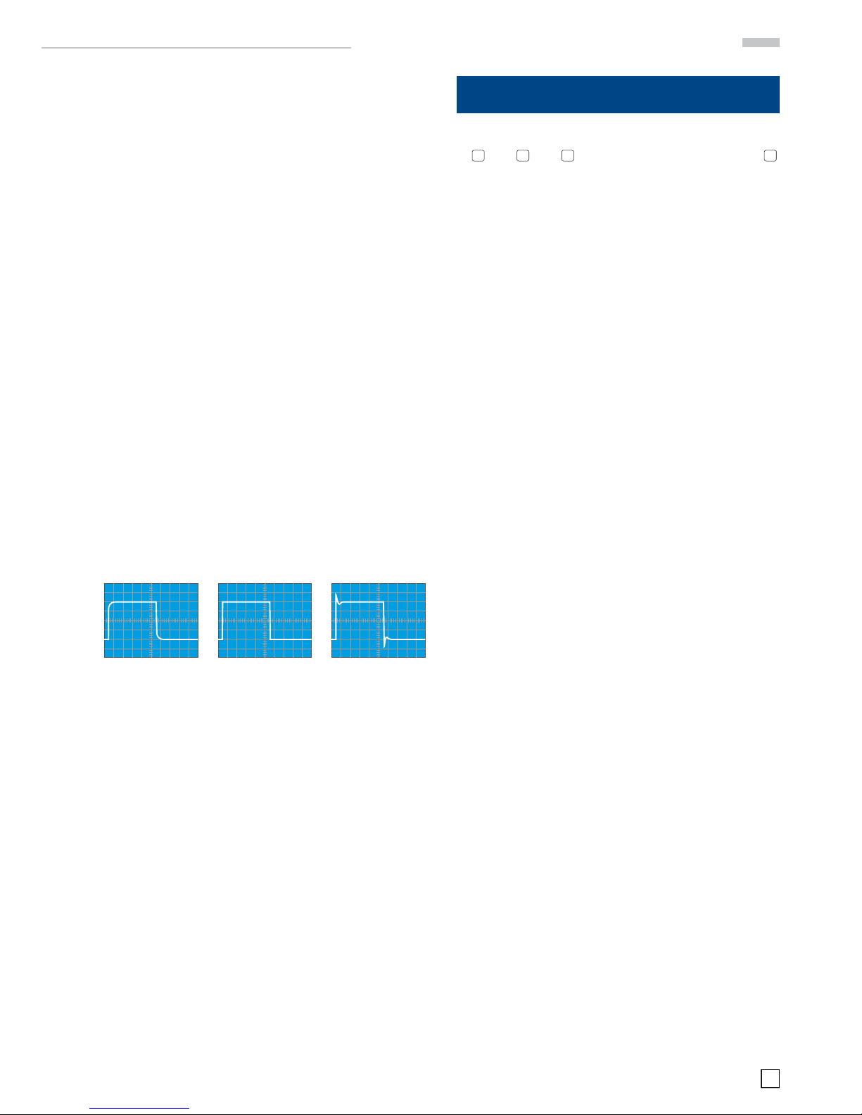
The criteria for a correct adjustment are:

– short rise time, steep slope.

– clean top left corner with minimum over- or undershoot,

fl at top.

After adjustment check the amplitude which should be the
same as with 1 kHz.

It is important to fi rst adjust 1 kHz, then 1 MHz. It may be ne­cessary to check the 1 kHz adjustment again.

Please note that the calibrator signals are not calibrated with
respect to frequency and thus must not be used to check the
time base accuracy, also their duty cycle may differ from 1:1.The
probe adjustment is completed if the pulse tops are horizontal
and the amplitude calibration is correct.

Operating modes of the vertical amplifier

incorrect correct incorrect

14

Subject to change without notice

they are within the permissible input signal range; this is the
case if they can be displayed in these modes. Only then switch
to ADD. If this precaution is disregarded grossly false displays
may result as the input range of one or both amplifi ers may
be exceeded.
Another precondition for obtaining true displays is the use of
two identical probes at both inputs. But note that normal probe
tolerances (percent) will cause the CM rejection to be expected
to be rather moderate. In order to obtain the best possible re­sults proceed as follows: First adjust both probes as carefully
as possible, then select the same sensitivity at both inputs and
then connect both probes to the output of a pulse generator
with suffi cient amplitude to yield a good display. Readjust one
(!) of the probe adjustment capacitors for a minimum of over­or undershoot. As there is no adjustment provided with which
the resistors can be matched a residual pulse signal will be
unavoidable.
When making difference measurements it is good practice
to fi rst connect the ground cables of the probes to the object
prior to connecting the probe tips. There may be high potentials
between the object and the scope. If a probe tip is connected
fi rst there is danger of overstressing the probe or/and the scope
inputs! Never perform difference measurements without both
probe ground cables connected.

XY operation

This mode is accessed by VERT/XY 32 > XY. In analog mode the
time base will be turned off. The channel 1 signal will defl ect in X
direction (X-INP. = horizontal input), hence the input attenuators,
the variable and the POSITION 1 control will be operative. The
HORIZONTAL control will also remain functional.

Channel 2 will defl ect in Y direction.

The x10 magnifi er will be inoperative in XY mode. Please note the
differences in the Y and X bandwidths, the X amplifi er has a lower
–3 dB frequency than the Y amplifi er. Consequently the phase
difference between X and Y will increase with frequency.

In XY mode the X signal (CH1 = X-INP). can not be inverted.

The XY mode may generate Lissajous fi gures which simplify
some measuring tasks and make others possible:

– Comparison of two signals of different frequency or adjust-

ment of one frequency until it is equal to the other resp.
becomes synchronized.

– This is also possible for multiples or fractions of one of the

frequencies.

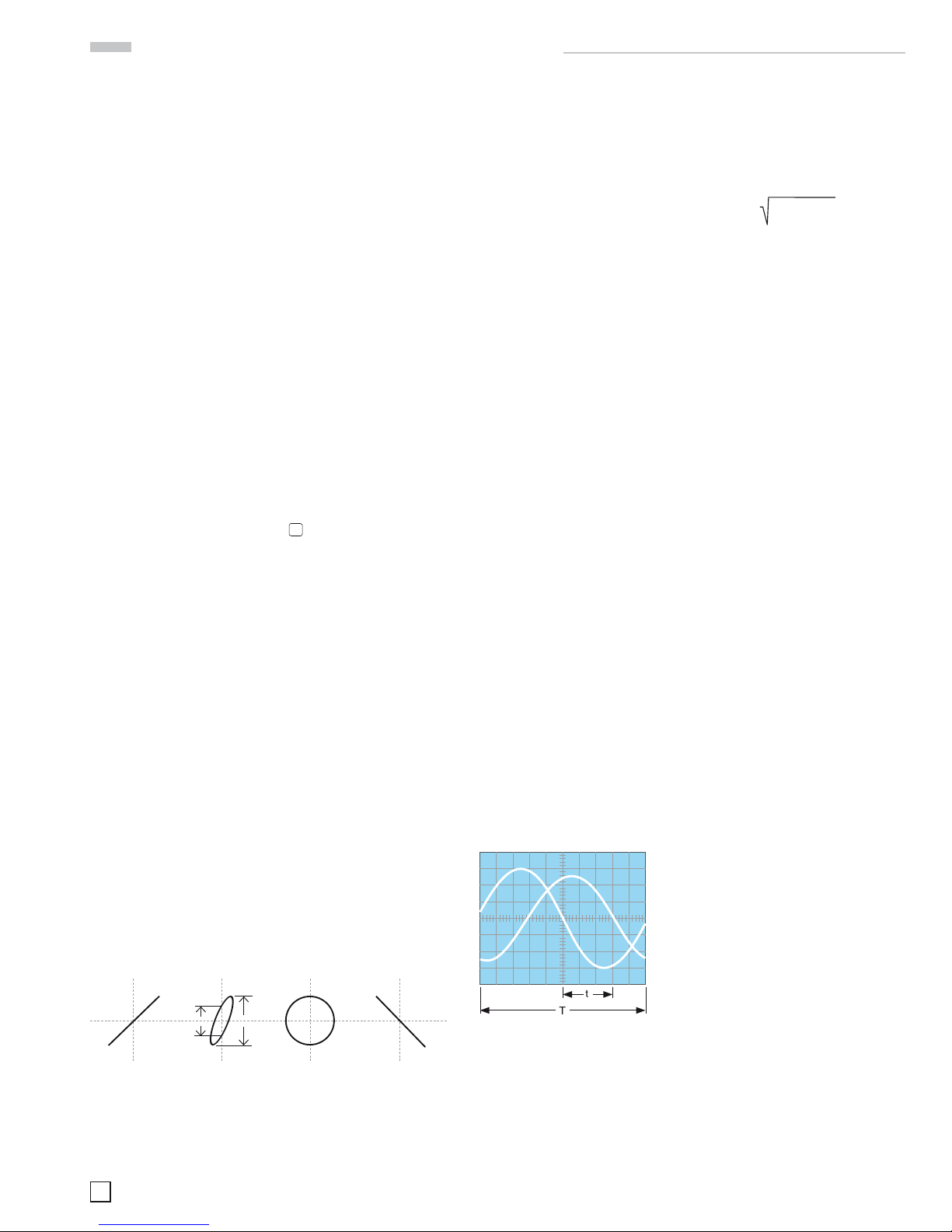
Phase measurements with Lissajous fi gures

The following pictures show two sine waves of equal amplitude
and frequency but differing phase.

0° 35° 90° 180°

ab

Calculation of the phase angle between the X- and Y-signals (af­ter reading a and b off the screen) is possible using the following
formulas and a pocket calculator with trigonometric functions.
This calculation is independent of the signal amplitudes:

Please note:

– As the trigonometric functions are periodic limit the calcu-

lation to angles <90 degrees. This is where this function is
most useful.

– Do not use too high frequencies,

because, as explained above, the
two amplifiers are not identical,
their phase difference increases
with frequency. The spec gives the
frequency at which the phase diffe­rence will stay <3 degrees.

– The display will not show which of the two frequencies does

lead or lag. Use a CR combination in front of the input of the
frequency tested. As the input has a 1 MΩ resistor it will be
suffi cient to insert a suitable capacitor in series. If the ellipse
increases with the C compared to the C short-circuited the
test signal will lead and vice versa. This is only valid <90
degrees. Hence C should be large and just create a barely
visible change.

If in XY mode one or both signals disappear, only a line or a point
will appear, mostly very bright. In case of only a point there is
danger of phosphor burn, so turn the intensity down immedia­tely; if only a line is shown the danger of burn will increase the
shorter the line is. Phosphor burn is permanent.

Measurement of phase differences in dual channel
Yt mode

Please note: Do not use ”alternate trigger“ because the time
differences shown are arbitrary and depend only on the respec­tive signal shapes! Make it a rule to use alternate trigger only
in rare special cases.
The best method of measuring time or phase differences is using
the dual channel Yt mode. Of course, only times may be read off
the screen, the phase must then be calculated as the frequency
is known. This is a much more accurate and convenient method
as the full bandwidth of the scope is used, and both amplifi ers
are almost identical. Trigger the time base from the signal
which shall be the reference. It is necessary to position both
traces without signal exactly on the graticule center (POSITION
1 and 2). The variables and trigger level controls may be used,
this will not infl uence the time difference measurement. For
best accuracy display only one period at high amplitude und
observe the zero crossings. One period equals 360 degrees. It
may be advantageous to use AC coupling if there is an offset
in the signals.

In this example t = 3 cm and T = 10 cm, the phase difference in
degrees will result from:

5 3
ϕ° =

—

· 360° = — · 360° = 108°

T 10

or in angular units:

t 3
arc ϕ° =

—

· 2π = — · 2π = 1,885 rad

T 10

Operating modes of the vertical amplifier

t = horizontal spacing of the zero

transitions in div

T= horizontal spacing for one

period in div

a
sin ϕ =

—

b

a
cos ϕ = 1 –

(—)

2

b

a
ϕ = arc sin

—

b

15

Subject to change without notice

Very small phase differences with moderately high frequencies
may yield better results with Lissajous fi gures.

However, in order to get higher precision it is possible to switch
to higher sensitivities – after accurately positioning at graticule
centre – thus overdriving the inputs resulting in sharper zero
crossings. Also, it is possible to use half a period over the full
10 cm. As the time base is quite accurate increasing the time
base speed after adjusting for e.g. one period = 10 cm and
positioning the fi rst crossing on the fi rst graticule line will also
give better resolution.

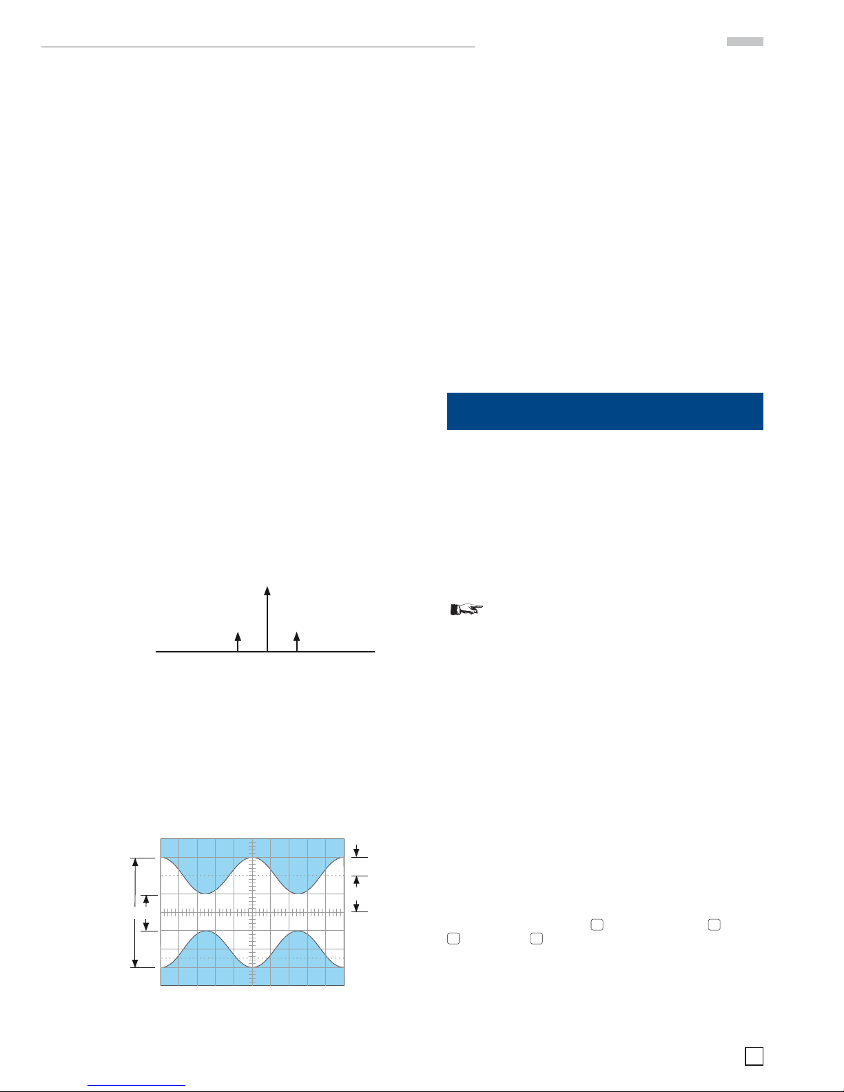
Measurement of amplitude modulation

Please note: Use this only in analog mode because in digital
mode alias displays may void the measurement! For the display
of low modulation frequencies a slow time base (TIME/DIV) has
to be selected in order to display one full period of the modu­lating signal. As the sampling frequency of any digital must be
reduced at slow time bases it may become too low for a true
representation.

The momentary amplitude at time t of a hf carrier frequency
modulated by a sinusoidal low frequency is given by:

u = UT · sinΩt + 0,5 m · UT · cos (Ω - ω) t - 0,5 m · UT · cos (Ω - ω) t

where: UT = amplitude of the unmodulated carrier
Ω = 2πF = angular carrier frequency
ω = 2πf = modulation angular frequency
m = modulation degree (≤1

v100%)

In addition to the carrier a lower side band F – f and an upper
side band F + f will be generated by the modulation.

Picture 1: Amplitudes and frequencies with AM (m = 50 %) of
the spectra

As long as the frequencies involved remain within the scope’s
bandwidth the amplitude-modulated hf can be displayed. Pre­ferably the time base is adjusted so that several signal periods
will be displayed. Triggering is best done from the modulation
frequency. Sometimes a stable displayed can be achieved by
twiddling with the time base variable.

Picture 2: Amplitude modulated hf. F = 1 MHz, f = 1 kHz,
m = 50 %, U

T

= 28,3 mV

rms

Set the scope controls as follows in order to display the picture
2 signal:

CH1 only, 20 mV/cm, AC
TIME/DIV: 0.2 ms/cm
Triggering: NORMAL, AC, internal.
Use the time base variable or external triggering.

Reading a and b off the screen the modulation degree will
result:

a – b a – b
m =

——

bzw. m =

—— · 100 [%]

a + b a + b

a = U

T

(1 + m) and b = UT (1 – m)

When measuring the modulation degree the amplitude and time
variables can be used without any infl uence on the result.

Triggering and time base

The most important controls and displays for these functions
are to be found in the shaded TRIGGER area, they are described
in „Controls and Readout“.-

In YT mode the signal will defl ect the trace vertically while the
time will defl ect it horizontally, the speed can be selected.
In general periodic voltage signals are displayed with a peri­odically repeating time base. In order to have a stable display
successive periods must trigger the time base at exactly the
same time position of the signal (amplitude and slope).

Pure DC can not trigger the time base, a voltage

change is necessary.

Triggering may be internal from any of the input signals or
externally from a time-related signal.

For triggering a minimum signal amplitude is required which
can be determined with a sine wave signal. With internal trigge­ring the trigger take-off within the vertical amplifi ers is directly
following the attenuators. The minimum amplitude is specifi ed
in mm on the screen. Thus it is not necessary to give a minimum
voltage for each setting of the attenuator.

For external triggering the appropriate input connector is used,
the amplitude necessary there is given in V

pp

. The voltage for
triggering may be much higher than the minimum, however, it
should be limited to 20 times the minimum. Please note that
for good triggering the voltage resp. signal height should be a
good deal above the minimum. The scope features two trigger
modes to be described in the following:

Automatic peak triggering (MODE menu)

Consult the chapters MODE 20 > AUTO, LEVEL A/B 19, FILTER

21

and SOURCE 22 in ”Controls and Readout“. Using AUTOSET
this trigger mode will be automatically selected. With DC coup­ling and with alternate trigger this mode will be left while the
automatic triggering will remain.

Automatic triggering causes a new time base start after the end
of the foregoing and after the hold-off time has elapsed even

Triggering and time base

F – f F F + f

0,5 m · U

T

0,5 m · U

T

U

T

ba

m · U

T

U

T