Fluke 718, 725, 753, 754, 707 Service Guide

Eliminating sensor

errors in loop

calibrations

Calibrating a loop is more than just

4 mA to 20 mA

Significant performance
improvement can realized by
optimizing the loop calibration
measurement system to better
accommodate the unique char­acteristics of the temperature
sensing element. All tempera­ture probes and their sensing
elements are unique, with
variations in materials, con­struction and usage, or exposure
to different environments. This
uniqueness continues through­out the useful life of the sensor,
in the form of drift due to
mechanical shock and vibra­tion or to contamination of the
materials when exposed to the
material they are measuring.
Only through periodic verifica­tion can these differences and
changes be accommodated,
improving total measurement
performance.

Temperature plays an impor­tant role in many industrial and
commercial processes. Examples
range from sterilization in
pharmaceutical companies,
metal heat-treatment to ensure
optimal strength in aerospace
applications, temperature
verification in a cold storage
warehouse, and atmospheric
and oceanographic research. In
all temperature measurement
applications, the sensor strongly
affects the results; unfortu­nately, many measurements are
made without optimizing the
system to get the best perfor­mance from the temperature
transducer.

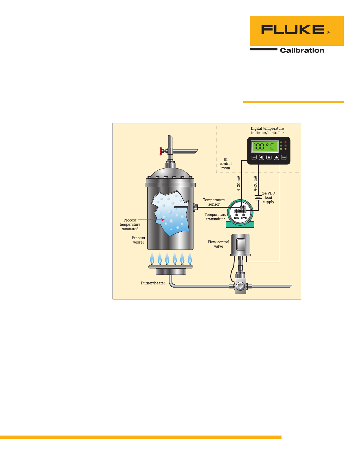
The majority of process
temperature measurements are
performed using a sensing ele­ment connected to a transmitter.

Figure 1. Diagram of a typical process temperature measurement system.

Figure 1 shows a diagram of a
common configuration.

In many applications, it is
common to verify the elements
of the measurement system
separately, but in doing so,
significant improvements made
possible by considering the
system as a whole are ignored.
One of the main reasons the
elements are verified or cali­brated separately is that it is
often considered to be more
efficient. Verifying the mea­surement component is done
simply and quickly with an
electronic thermocouple (TC) or

Application Note

resistance temperature detector
(RTD) simulator. This approach
does not verify the performance
of the associated temperature
probe, and assumes all probes
are identical and closely follow
some standard. In practice, no
two probes are identical; they
all vary from the ideal standard,
and over time and usage their
characteristics change. Under­standing how probes vary from
the ideal will allow you to opti­mize the measurement system
to achieve the best performance.

From the Fluke Calibration Digital Library @ www.flukecal.com/library

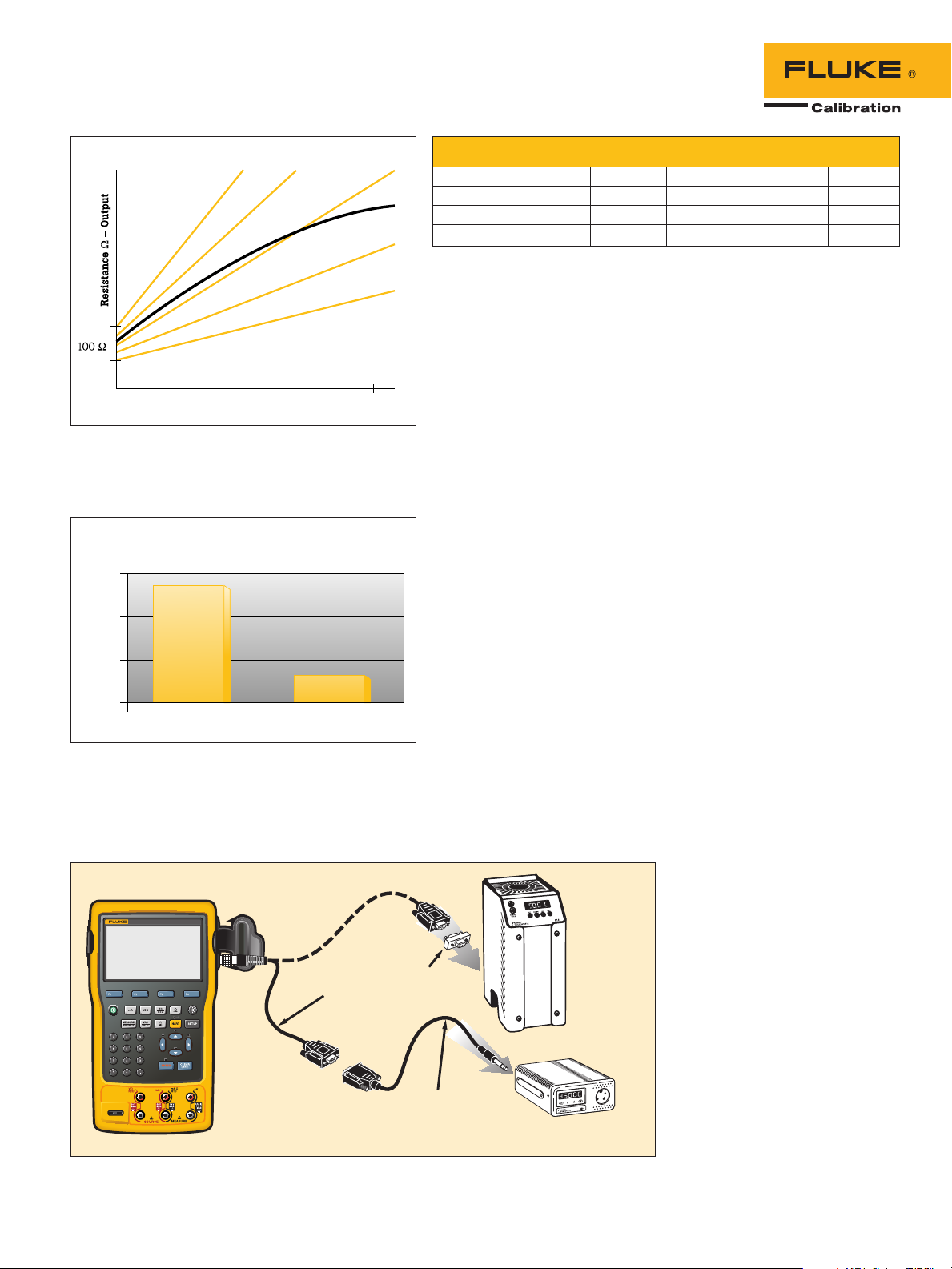
Ideal curve

Actual curve

Class A tolerance

Class B tolerance

0 °C 400 °C

Figure 2.

System accuracy improved by more than 75 %!

1.2

0.8

0.4

RSS Error ± °C

0

Figure 3. System accuracy improvement achieved with a
calibrated Pt100 Sensor.

DOCUMENTING PROCESS CALIBRATOR

754

Figure 4. Connecting a Fluke 754 to a Fluke Calibration dry-well.

Temperature °C – Input

Standard Sensor Calibrated Sensor

2514 dry-well

interface cable

System accuracy comparison measuring 150 °C using a Pt100 (IEC751)
RTD with a transmitter span of 0 to 200 °C

Standard RTD Accuracy Characterized RTD Accuracy
Rosemount Model 644H ± 0.15 °C Rosemount Model 644H ± 0.15 °C
Standard RTD ± 1.05 °C Matched (calibrated) RTD ± 0.18 °C
Total system ± 1.06 °C Total system ± 0.23 °C

Total system accuracy calculated using RSS statistical method.

Table 1

Rosemount Inc. uses the
example provided in Table 1 for
information on the possible per­formance improvement of their
Model 644H Smart Tempera­ture Transmitter. To achieve
this performance improvement,
the Rosemount 644H is given
information (Callendar Van
Dusen Coefficients) that allows
it to correct for the unique
performance of the temperature
sensing element, in this case a
standard IEC751 Pt100 sensor.

Dry-wells and micro-baths
are good choices for verifying
the performance of tempera­ture probes and other related
sensors. But they do not have
the capability to calibrate the
transmitter’s output or read­out and, by themselves, do
not allow the entire measure­ment loop to be optimized. A
heat source, combined with an
intelligent electronic process
calibrator that is capable of
calibrating the transmitter and
readout, is required if the above
performance improvement is to
be realized and maintained.

By combining the automating
and documenting capabilities
of the Fluke 754 Document­ing Process Calibrator with
Fluke Calibration’s intelligent
and stable family of field dry­wells and micro-baths, you
have the capability to test the
entire loop. This combination of
equipment allows you to easily
verify the characteristics of the
temperature sensor and mea­surement electronics. Using this
information, the entire loop can
be adjusted to optimize system
measurement performance.
Below are some examples of
how to optimize the perfor­mance of your measurement
system using these instruments.

The Fluke 754 is connected
to a Fluke Calibration dry-well
or micro-bath by way of a serial
RS-232 interface cable. Version

2.3 or greater firmware for the
754 is required. The firmware
version is displayed briefly on
the display of the 754 during
power-up. If you do not have
the required firmware, contact
your authorized Fluke distribu­tor for information regarding an
upgrade. The serial cable may
be obtained from either your
authorized Fluke distributor or
directly from your Fluke Calibra­tion representative. The heat

Null modem

Fluke Calibration

Dry-well

(DB9)

source is connected to the 754
pressure port and is accessed
by the 754 TC/RTD source
key. Due to the length of these
tests, it is recommended that a
fully charged battery or battery
eliminator for the 754 be used.
A diagram of the connection of

Fluke Calibration

3.5 mm

interface cable

Fluke Calibration

Dry-well (3.5 mm)

this equipment is pictured in
Figure 4.

In many process applications,
the instrumentation of choice
for temperature measurements

2 Fluke Corporation Eliminating sensor errors in loop calibrations

is a transmitter that accepts the
output from the temperature
sensor and drives a 4-20 mA
signal back to the PLC, DCS or
indicator. This example describes
one method for verifying per­formance and offers to optimize
this measurement to improve
performance.

To perform this test, the RTD
sensor is removed from the
process and inserted in to the
dry-block calibrator. The mA
connections from the transmit­ter are connected directly to
the 754 Documenting Process
Calibrator (see Figure 5). In
most applications, this solution
provides adequate performance.
But if your application includes
a uniquely-shaped sensor, you
might want to consider the use
of a micro-bath. If increased
heat source accuracy is needed,
the use of a reference thermom­eter combined with the 754’s
User-Entered Values feature can
be used. See application note
1263925 for more information
on 754 User-Entered Values.

Once connections are made,
you are ready to acquire trans­mitter configuration (if you
have a transmitter with HART
communications), set the test
parameters, and configure the
calibrator for mA measurement
and dry-well control as the
sourcing parameter.

Pressing the HART key on
the 754 allows the calibra­tor to acquire the transmitter
configuration from a transmit­ter with HART communication
capability. Following is a sample
of this acquired configuration
information.

Pressing the HART key on
the 754 again presents the
following screen with several
options for configuring the cali­brator to the correct parameters
for this test. For the purposes
of this example, we’ll use the
transmitter configured to output
a 4-20mA signal; therefore the
correct configuration of the 754
is to measure mA and source
temperature via the dry-well.

Pressing the AS FOUND soft
key on the 754 provides access
to parameters needed to con­figure an automated test. Below
is a typical definition that will
test the measurement system
from 50°C to 150°C sourcing
temperatures using a dry-well

in ascending order.

After the test has been
defined, the Fluke 754 will take
over and run the test record­ing the sourced temperature,
measured output of the trans­mitter, in mA. At the end of the
test, the results will be dis­played on the screen, allowing
the test technician to evaluate
the results and take corrective
action if needed. Following is

Figure 5. Fluke 754 and Fluke Calibration dry-well calibrating a
4-20 mA transmitter and temperature sensor.

an example of the results.

One method of optimizing
this system to minimize error
is to shift the URV or LRV of
the transmitter to the values
measured by the 754. With a
transmitter with HART capa­bilities, this is easily done via
the 754, by simply entering
new values in the HART SETUP

3 Fluke Corporation Eliminating sensor errors in loop calibrations

screen below. With an analog
transmitter, you will need to
mechanically adjust the Zero
and Span adjustments when
sourcing the appropriate tem­perature values. The 754 has
a convienent menu key that
allows you to easily set the cor­rect value on the dry-well with
a single button press.

a sensor and the ability to
perform curve-fitting of the
collected data.

The method of character­izing a probe is similar to the
procedure above, but rather
than measuring the output of
the transmitter, the output of
the sensor is connected directly
to the 754. An example of data
collected by a 754 on a temper-

Calibrating and adjusting
measurement systems using
characterized sensors and

ature sensor is shown below.

Data like this can be entered

calibration constants

Another method of reducing
uncertainty and optimizing tem­perature measurement systems
is to carefully characterize the
temperature sensor, calculate
correction coefficients and load
these correction coefficients into
the measurement equipment.
This is the method used in the
Rosemount 644H example on
the previous page. This method
does a better job of reducing
the error in the measurement
system that comes from the
sensor. But it requires trans­mitters that have a correction

into Fluke Calibration’s software
using the screens in Figure 6
and then unique CVD constants
calculated for that probe.

These coefficients can then
be entered into a suitable
measurement device that allows
its linearizations to match the
characteristics of the probe.

or linearization algorithm that
can accommodate the sensor.
For example, Platinum RTDs
typically use the Callendar­Van Dusen (CVD) equation for
linearizing the sensor’s output.
A characterized sensor will
provide unique CVD coefficients
that can be input into the trans­mitter, allowing its conversion
algorithm to more closely match
the unique characteristics of the

Summary

Using a dry-well in combina­tion with a process calibrator
allows measurement systems
to be verified and adjusted to
optimize measurement perfor­mance. By verifying the entire
measurement system, unique
characteristics of the sensing
element can be combined with
the measurement electronics

sensor.

The Fluke 754 connected
with a dry-well can help
to collect the necessary
information to characterize the
sensor, but additional software
and resources will be needed
to take this data and generate
new CVD constants. Examples
of the required software include
Fluke Calibration’s TableWare.
Other software that could
be used include Mathcad,
Mathematica, Maple or Excel.
But these packages require
considerable knowledge of
the equations used to linearize

4 Fluke Corporation Eliminating sensor errors in loop calibrations

Figure 6. TableWare software from Fluke Calibration calculates unique
CVD constants that match the characteristics of the probe.

to minimize measurement
error. This can result in a
significant reduction in mea­surement errors. The Fluke 754
Documenting Process Calibra­tor, combined with a Fluke
Calibration dry-well makes this
process faster and easier.

Fluke Calibration. Precision, performance, confidence.

Fluke Calibration
PO Box 9090,
Everett, WA 98206 U.S.A.

For more information call:
In the U.S.A. [phone] or Fax [phone]
In Europe/M-East/Africa [phone] or Fax [phone]
In Canada (800)-36-FLUKE or Fax [phone]
From other countries [phone] or Fax [phone]
Web access: http://www.flukecal.com

©2004-2011 Fluke Corporation. Specifications subject to change without notice.
Printed in U.S.A. 11/2011 2148146C A-EN-N

Modification of this document is not permitted without written permission from Fluke Corporation.

Fluke Europe B.V.

PO Box 1186, 5602 BD
Eindhoven, The Netherlands

™