Fluke 19xC-2x5C ScopeMeter User manual

Fluke 19xC-2x5C

ScopeMeter

Software version 8.00 onwards

Users Manual

4822 872 30805
July 2008

© 2008 Fluke Corporation. All rights reserved.
All product names are trademarks of their respective companies.

LIMITED WARRANTY & LIMITATION OF LIABILITY

Each Fluke product is warranted to be free from defects in material and workmanship under normal use and service. The warranty period is three years for the
test tool and one year for its accessories. The warranty period begins on the date of shipment. Parts, product repairs and services are warranted for 90 days.
This warranty extends only to the original buyer or end-user customer of a Fluke authorized reseller, and does not apply to fuses, disposable batteries or to any
product which, in Fluke's opinion, has been misused, altered, neglected or damaged by accident or abnormal conditions of operation or handling. Fluke
warrants that software will operate substantially in accordance with its functional specifications for 90 days and that it has been properly recorded on non­defective media. Fluke does not warrant that software will be error free or operate without interruption.

Fluke authorized resellers shall extend this warranty on new and unused products to end-user customers only but have no authority to extend a greater or different
warranty on behalf of Fluke. Warranty support is available if product is purchased through a Fluke authorized sales outlet or Buyer has paid the applicable
international price. Fluke reserves the right to invoice Buyer for importation costs of repair/replacement parts when product purchased in one country is submitted for
repair in another country.

Fluke's warranty obligation is limited, at Fluke's option, to refund of the purchase price, free of charge repair, or replacement of a defective product which is returned to
a Fluke authorized service center within the warranty period.

To obtain warranty service, contact your nearest Fluke authorized service center or send the product, with a description of the difficulty, postage and insurance
prepaid (FOB Destination), to the nearest Fluke authorized service center. Fluke assumes no risk for damage in transit. Following warranty repair, the product will be
returned to Buyer, transportation prepaid (FOB Destination). If Fluke determines that the failure was caused by misuse, alteration, accident or abnormal condition of
operation or handling, Fluke will provide an estimate of repair costs and obtain authorization before commencing the work. Following repair, the product will be
returned to the Buyer transportation prepaid and the Buyer will be billed for the repair and return transportation charges (FOB Shipping Point).

THIS WARRANTY IS BUYER'S SOLE AND EXCLUSIVE REMEDY AND IS IN LIEU OF ALL OTHER WARRANTIES, EXPRESS OR IMPLIED, INCLUDING BUT
NOT LIMITED TO ANY IMPLIED WARRANTY OF MERCHANTABILITY OR FITNESS FOR A PARTICULAR PURPOSE. FLUKE SHALL NOT BE LIABLE FOR ANY
SPECIAL, INDIRECT, INCIDENTAL OR CONSEQUENTIAL DAMAGES OR LOSSES, INCLUDING LOSS OF DATA, WHETHER ARISING FROM BREACH OF
WARRANTY OR BASED ON CONTRACT, TORT, RELIANCE OR ANY OTHER THEORY.

Since some countries or states do not allow limitation of the term of an implied warranty, or exclusion or limitation of incidental or consequential damages, the
limitations and exclusions of this warranty may not apply to every buyer. If any provision of this Warranty is held invalid or unenforceable by a court of competent
jurisdiction, such holding will not affect the validity or enforceability of any other provision.

Fluke Corporation, P.O. Box 9090, Everett, WA 98206-9090 USA, or

Fluke Industrial B.V., P.O. Box 90, 7600 AB, Almelo, The Netherlands

SERVICE CENTERS

To locate an authorized service center, visit us on the World Wide Web:

http://www.fluke.com

or call Fluke using any of the phone numbers listed below:

[phone] in U.S.A. and Canada

[phone] in Europe

[phone] from other countries

Table of Contents

Chapter Title Page

Unpacking the Test Tool Kit........................................................................................ 0-2

Safety Information: Read First .................................................................................... 0-4

1 Using The Scope....................................................................................................... 1-7

Powering the Test Tool ............................................................................................... 1-7

Resetting the Test Tool............................................................................................... 1-8

Navigating a Menu ...................................................................................................... 1-9

Hiding Key Labels and Menus .................................................................................... 1-10

Input Connections ....................................................................................................... 1-10

Making Scope Connections ........................................................................................ 1-11

Displaying an Unknown Signal with Connect-and-View™........................................... 1-12

Making Automatic Scope Measurements.................................................................... 1-13

Freezing the Screen.................................................................................................... 1-14

Using Average, Persistence and Glitch Capture ......................................................... 1-15

Acquiring Waveforms.................................................................................................. 1-18

Pass - Fail Testing ...................................................................................................... 1-24

Analyzing Waveforms ................................................................................................. 1-25

i

Fluke 19xC-2x5C

Users Manual

2 Using The Multimeter ............................................................................................... 2-27

Making Meter Connections ......................................................................................... 2-27

Making Multimeter Measurements.............................................................................. 2-28

Freezing the Readings................................................................................................ 2-31

Selecting Auto/Manual Ranges................................................................................... 2-31

Making Relative Measurements.................................................................................. 2-32

3 Using The Recorder Functions ............................................................................... 3-33

Opening the Recorder Main Menu.............................................................................. 3-33

Plotting Measurements Over Time (TrendPlot™) ....................................................... 3-34

Recording Scope Waveforms In Deep Memory (Scope Record)................................ 3-37

Analyzing a TrendPlot or Scope Record..................................................................... 3-40

4 Using Replay, Zoom and Cursors ........................................................................... 4-41

Replaying the 100 Most Recent Scope Screens......................................................... 4-41

Zooming in on a Waveform......................................................................................... 4-44

Making Cursor Measurements.................................................................................... 4-46

5 Triggering on Waveforms ........................................................................................ 5-51

Setting Trigger Level and Slope.................................................................................. 5-52

Using Trigger Delay or Pre-trigger .............................................................................. 5-53

Automatic Trigger Options .......................................................................................... 5-54

Triggering on Edges ................................................................................................... 5-55

Triggering on External Waveforms ............................................................................. 5-58

Triggering on Video Signals........................................................................................ 5-59

Triggering on Pulses................................................................................................... 5-61

ii

Contents

6 Using The Bushealth Function................................................................................ 6-65

Bushealth Function Availability ................................................................................... 6-65

Introduction ................................................................................................................. 6-65

Performing Bushealth Measurements......................................................................... 6-66

Reading the Screen .................................................................................................... 6-68

Input Connections and Tested Signals ....................................................................... 6-70

Viewing the Bus Waveform Screen............................................................................. 6-80

Setting the Test Limits ................................................................................................ 6-81

Saving and Recalling Test Limits ................................................................................ 6-82

7 Using Memory, PC and Printer ................................................................................ 7-83

Saving and Recalling .................................................................................................. 7-83

Documenting Screens................................................................................................. 7-88

8 Tips ............................................................................................................................ 8-91

Using the Standard Accessories ................................................................................. 8-91

Using the Independently Floating Isolated Inputs ....................................................... 8-93

Using the Tilt Stand..................................................................................................... 8-95

Resetting the Test Tool............................................................................................... 8-95

Suppressing Key Labels and Menu’s.......................................................................... 8-95

Changing the Information Language........................................................................... 8-96

Adjusting the Contrast and Brightness........................................................................ 8-96

Changing the Display Color ........................................................................................ 8-97

Changing Date and Time ............................................................................................ 8-97

Saving Battery Life...................................................................................................... 8-98

Changing the Auto Set Options................................................................................... 8-99

9 Maintaining the Test Tool......................................................................................... 9-101

(continued)

iii

Fluke 19xC-2x5C

Users Manual

Cleaning the Test Tool................................................................................................ 9-101

Storing the Test Tool .................................................................................................. 9-101

Charging the Batteries ................................................................................................ 9-102

Extending Battery Operation Time.............................................................................. 9-103

Replacing the NiMH Battery Pack BP190................................................................... 9-104

Calibrating the Voltage Probes ................................................................................... 9-104

Displaying Calibration Information .............................................................................. 9-106

Parts and Accessories ................................................................................................ 9-106

Troubleshooting .......................................................................................................... 9-111

10 Specifications ........................................................................................................... 10-113

Introduction................................................................................................................. 10-113

Dual Input Oscilloscope .............................................................................................. 10-114

Automatic Scope Measurements ................................................................................ 10-116

Meter .......................................................................................................................... 10-120

DMM Measurements on Meter Inputs......................................................................... 10-120

Recorder..................................................................................................................... 10-122

Zoom, Replay and Cursors......................................................................................... 10-123

Fieldbus – Bushealth .................................................................................................. 10-123

Miscellaneous ............................................................................................................. 10-124

Environmental............................................................................................................. 10-125

Safety.................................................................................................................. 10-126

10:1 Probe .................................................................................................................. 10-127

Electromagnetic Immunity........................................................................................... 10-129

Appendices

iv

Contents

A Bushealth Measurements .................................................................................... A-1

(continued)

v

Unpacking the Test Tool Kit

Declaration of Conformity

for

Fluke 192C - 196C - 199C – 215C – 225C

ScopeMeter

Manufacturer

Fluke Industrial B.V.

7602 EA Almelo

The Netherlands

Statement of Conformity

Based on test results using appropriate standards,

the product is in conformity with

Electromagnetic Compatibility Directive 2004/108/EC

Low Voltage Directive 2006/95/EC

®

test tools

Lelyweg 14

Sample tests

Standards used:

EN 61010.1 : 2001

Safety Requirements for Electrical Equipment for

Measurement, Control, and Laboratory Use

EN61326-1:2006

Electrical equipment for

measurements and laboratory

use -EMC requirements-

The tests have been performed in a

typical configuration.

This Conformity is indicated by the symbol

i.e. “Conformité Européenne”.

,

1

Fluke 19xC-2x5C

Users Manual

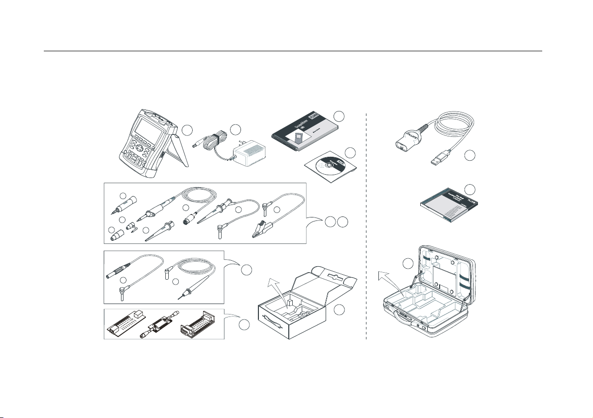
Unpacking the Test Tool Kit

The following items are included in your test tool kit:

1

(2x)

e

(2x)

f

(2x)

g

(2x)

b

b

(2x)

a

(2x)

a

2

(2x)

c

5

6

Figure 1. ScopeMeter Test Tool Kit

Note

When new, the rechargeable NiMH battery is not
fully charged. See Chapter 9.

7

8

(2x)

d

3

4

12

9

10

11

2

Unpacking the Test Tool Kit

# Description

1 ScopeMeter Test Tool

2 Battery Charger (country dependent)

3 10:1 Voltage Probe Set (red)

a) 10:1 Voltage Probe (red)
b) Hook Clip for Probe Tip (red)
c) Ground Lead with Hook Clip (red)
d) Ground Lead with Mini Alligator Clip (black)
e) 4-mm Test Probe for Probe Tip (red)
f) Ground Spring for Probe Tip (black)

g) Insulation Sleeve (red)

4 10:1 Voltage Probe Set (gray)

a) 10:1 Voltage Probe (gray)
b) Hook Clip for Probe Tip (gray)
c) Ground Lead with Hook Clip (gray)
d) Ground Lead with Mini Alligator Clip (black)

e) 4-mm Test Probe for Probe Tip (gray)
f) Ground Spring for Probe Tip (black)
g) Insulation Sleeve (grey)

a) Test Lead Set

5

b) Probe ground lead with 4 mm banana jack

6 BHT190 Bus Health Test adapter (2x5C only)

7 Getting Started Manual

8 CD ROM with Users Manual (multi-language)

9 Shipment box (basic version only)

Fluke 19xC and 2x5C -S versions include also the
following items:

# Description

10 Optically Isolated USB Adapter/Cable

11 FlukeView® ScopeMeter® Software for

Windows®

12 Hard Case

3

Fluke 19xC-2x5C

Users Manual

Safety Information: Read First

Carefully read the following safety information before using
the test tool.

Specific warning and caution statements, where they
apply, appear throughout the manual.

A “Warning” identifies conditions and actions
that pose hazard(s) to the user.

A “Caution” identifies conditions and actions
that may damage the test tool.

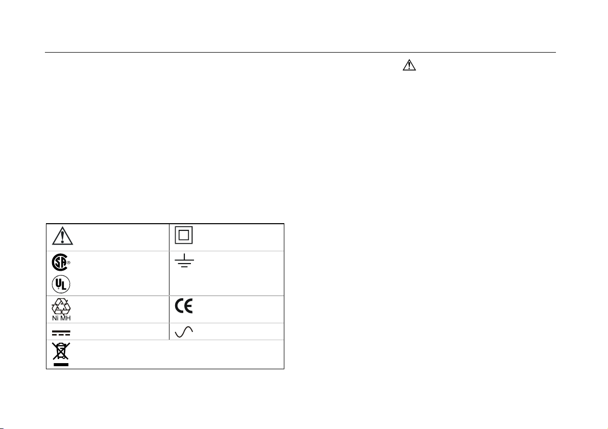
The following international symbols are used on the test
tool and in this manual:

See explanation in
manual

Safety Approval

Recycling information

Direct Current

Do not dispose of this product as unsorted municipal
waste. Go to Fluke's website for recycling information.

Double Insulation
(Protection Class)

Earth ground

Conformité
Européenne

Alternating Current

Warning

To avoid electrical shock or fire:

• Use only the Fluke power supply, Model

BC190 (Battery Charger / Power Adapter).

• Before use check that the selected/indicated

range on the BC190 matches the local line
power voltage and frequency.

• For the BC190/808 universal Battery Charger /

Power Adapter) only use line cords that
comply with the local safety regulations.

Note:

To accomodate connection to various line power
sockets, the BC190/808 universal Battery
Charger / Power Adapter is equipped with a male
plug that must be connected to a line cord
appropriate for local use. Since the adapter is
isolated, the line cord does not need to be
equipped with a terminal for connection to
protective ground. Since line cords with a
protective grounding terminal are more commonly
available you might consider using these anyhow.

4

Safety Information: Read First

Warning

To avoid electrical shock or fire if a test tool
input is connected to more than 42 V peak (30
Vrms) or on circuits of more than 4800 VA:

• Use only insulated voltage probes, test leads

and adapters supplied with the test tool, or
indicated by Fluke as suitable for the Fluke
19xC – 2x5C ScopeMeter series.

• Before use, inspect voltage probes, test leads

and accessories for mechanical damage and
replace when damaged.

• Remove all probes, test leads and accessories

that are not in use.

• Always connect the battery charger first to the

ac outlet before connecting it to the test tool.

• Do not connect the ground spring (figure 1,

item f) to voltages higher than 42 V peak (30
Vrms) from earth ground.

• Do not apply voltages that differ more than 600

V from earth ground to any input when
measuring in a CAT III environment.
Do not apply voltages that differ more than
1000 V from earth ground to any input when
measuring in a CAT II environment.

• Do not apply voltages that differ more than 600

V from each other to the isolated inputs when
measuring in a CAT III environment.
Do not apply voltages that differ more than
1000 V from each other to the isolated inputs
when measuring in a CAT II environment.

• Do not apply input voltages above the rating of

the instrument. Use caution when using 1:1
test leads because the probe tip voltage will be
directly transmitted to the test tool.

• Do not use exposed metal BNC or banana plug

connectors.

• Do not insert metal objects into connectors.

• Always use the test tool only in the manner

specified.

Voltage ratings that are mentioned in the warnings, are
given as limits for “working voltage”. They represent
V ac rms (50-60 Hz) for ac sinewave applications and as V
dc for dc applications.

Measurement Category III refers to distribution level and
fixed installation circuits inside a building.
Measurement Category II refers to local level, which is
applicable for appliances and portable equipment.

5

Fluke 19xC-2x5C

Users Manual

The terms ‘Isolated’ or ‘Electrically floating’ are used in this
manual to indicate a measurement in which the test tool
input BNC or banana jack is connected to a voltage
different from earth ground.

The isolated input connectors have no exposed metal and
are fully insulated to protect against electrical shock.

The red and gray BNC jacks, and the red and black
4-mm banana jacks can independently be connected to a
voltage above earth ground for isolated (electrically
floating) measurements and are rated up to 1000 Vrms
CAT II and 600 Vrms CAT III above earth ground.

If Safety Features are Impaired

Use of the test tool in a manner not specified may
impair the protection provided by the equipment.

Before use, inspect the test leads for mechanical damage
and replace damaged test leads!

Whenever it is likely that safety has been impaired, the
test tool must be turned off and disconnected from the line
power. The matter should then be referred to qualified
personnel. Safety is likely to be impaired if, for example,
the test tool fails to perform the intended measurements or
shows visible damage.

6

About this Chapter

This chapter provides a step-by-step introduction to the
scope functions of the test tool. The introduction does not
cover all of the capabilities of the scope functions but gives
basic examples to show how to use the menus and
perform basic operations.

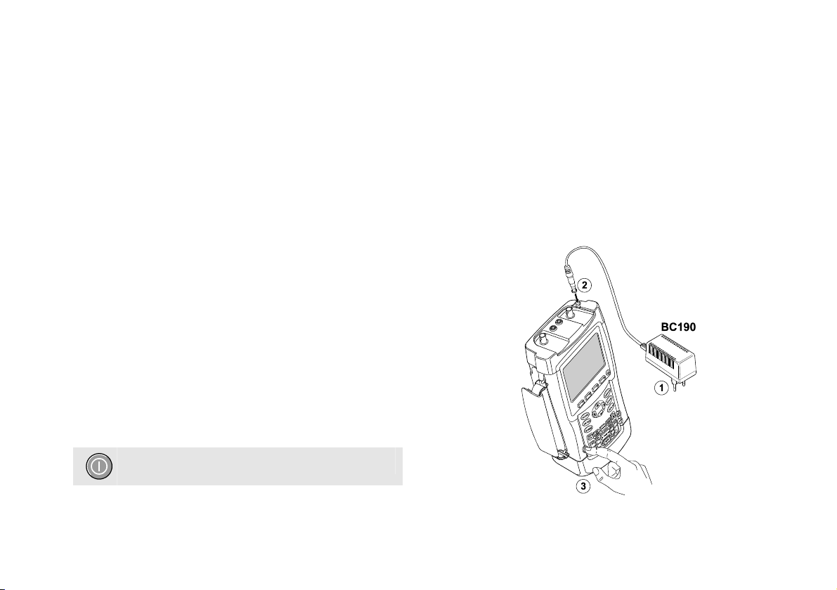
Powering the Test Tool

Follow the procedure (steps 1 through 3) in Figure 2 to
power the test tool from a standard ac outlet.
See Chapter 8 for instructions on using battery power.

Turn the test tool on with the on/off key.

The test tool powers up in its last setup configuration.

Chapter 1

Using The Scope

Figure 2. Powering the Test Tool

7

Fluke 19xC-2x5C

Users Manual

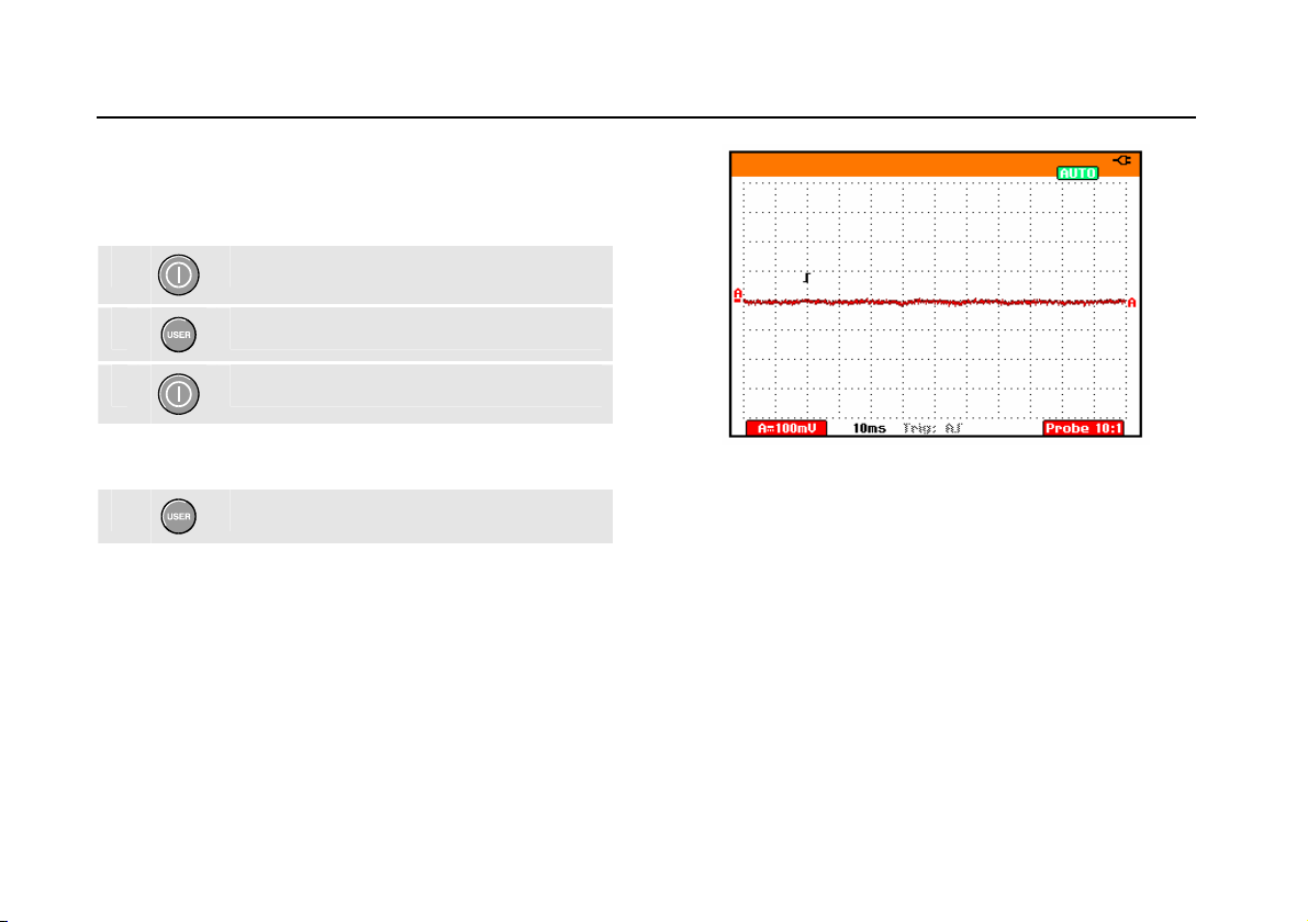
Resetting the Test Tool

If you want to reset the test tool to the factory settings, do
the following:

1

Turn the test tool off.

2

3

Press and hold the USER key.

Press and release.

The test tool turns on, and you should hear a double beep,
indicating the reset was successful.

4

Now look at the display; you will see a screen that looks
like

Figure 3.

8

Release the USER key.

Figure 3. The Screen After Reset

Using The Scope
Navigating a Menu

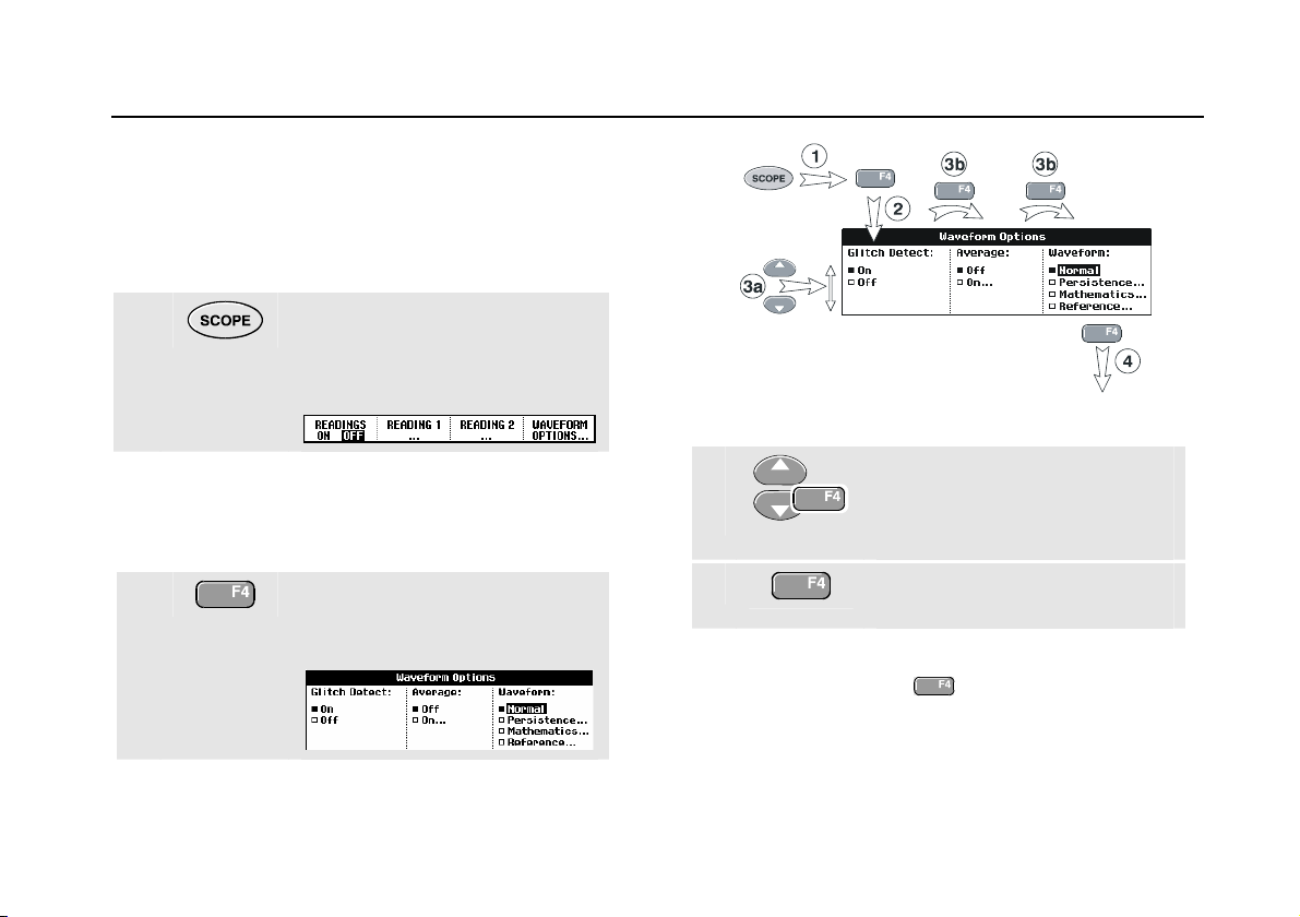
Navigating a Menu

The following example shows how to use the test tool's
menus to select a function. Subsequently follow steps
1 through 4 to open the scope menu and to choose an
item.

1

1

Press the SCOPE key to display
the labels that define the present
use for the four blue function keys
at the bottom of the screen.

Figure 4. Basic Navigation

Note

To hide the labels for full screen view, press the

SCOPE key again. This toggling enables you to

check the labels without affecting your settings.

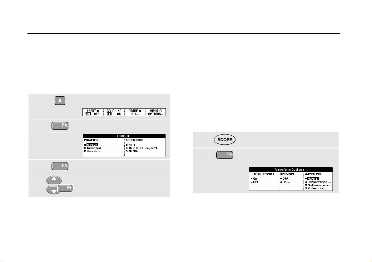
2

Open the Waveform Options
menu. This menu is displayed at
the bottom of the screen.

3a

3b

4

Repeatedly pressing
through a menu without changing the settings.

9

Use the blue arrow keys to
highlight the item.
Press the blue ENTER key to
accept the selection.

Press the ENTER key until you exit
the menu.

Note

lets you to step

Fluke 19xC-2x5C

Users Manual

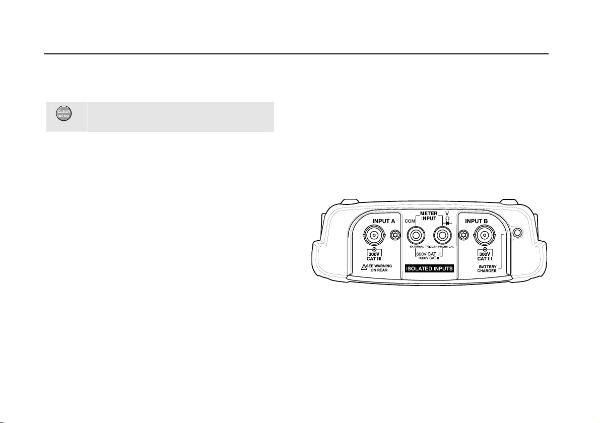
Hiding Key Labels and Menus

You can hide a menu or key label at any time:

Press the CLEAR MENU key to hide any key
label or menu.

To display menus or key labels, press one of the yellow
menu keys, e.g. the SCOPE key.

Input Connections

Look at the top of the test tool. The test tool has four
signal inputs: two safety BNC jack inputs (red input A and
gray input B) and two safety 4-mm banana jack inputs (red
and black). Use the two BNC jack inputs for scope
measurements, and the two banana jack inputs for meter
measurements.

Isolated input architecture allows independent floating
measurements with each input.

Figure 5. Measurement Connections

10

Using The Scope
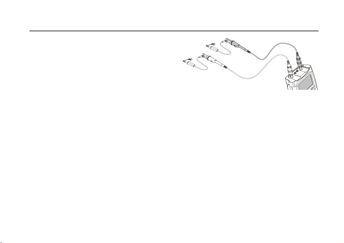
Making Scope Connections

Making Scope Connections

To make dual input scope measurements, connect the red
voltage probe to input A, and the gray voltage probe to
input B. Connect the short ground leads of each voltage
probe to its own reference potential. (See

Figure 6.)

1

Note

To maximally benefit from having independently
isolated floating inputs and to avoid problems
caused by improper use, read Chapter 8: “Tips”.

11

Figure 6. Scope Connections

Fluke 19xC-2x5C

Users Manual

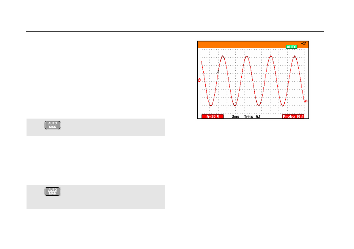
Displaying an Unknown Signal with Connect-and-View™

The Connect-and-View feature lets the test tool display
complex, unknown signals automatically. This function
optimizes the position, range, time base, and triggering
and assures a stable display of virtually any waveform. If
the signal changes, the setup is automatically adjusted to
maintain the best display result. This feature is especially
useful for quickly checking several signals.

To enable the Connect-and-View feature, do the following:

1

Perform an Auto Set. AUTO appears at
the top right of the screen.

Figure 7. The Screen After an Auto Set

The bottom line shows the range, the time base, and the
trigger information.

The waveform identifier (A) is visible on the bottom right
side of the screen, as shown in
icon (-) at the left side of the screen identifies the ground
level of the waveform.

2

Press a second time to select the
manual range again. MANUAL appears
at the top right of the screen.

Figure 7. The input A zero

12

Use the light-gray
bottom of the keypad to change the view of the waveform
manually.

RANGE, TIME and MOVE keys at the

Using The Scope
Making Automatic Scope Measurements

1

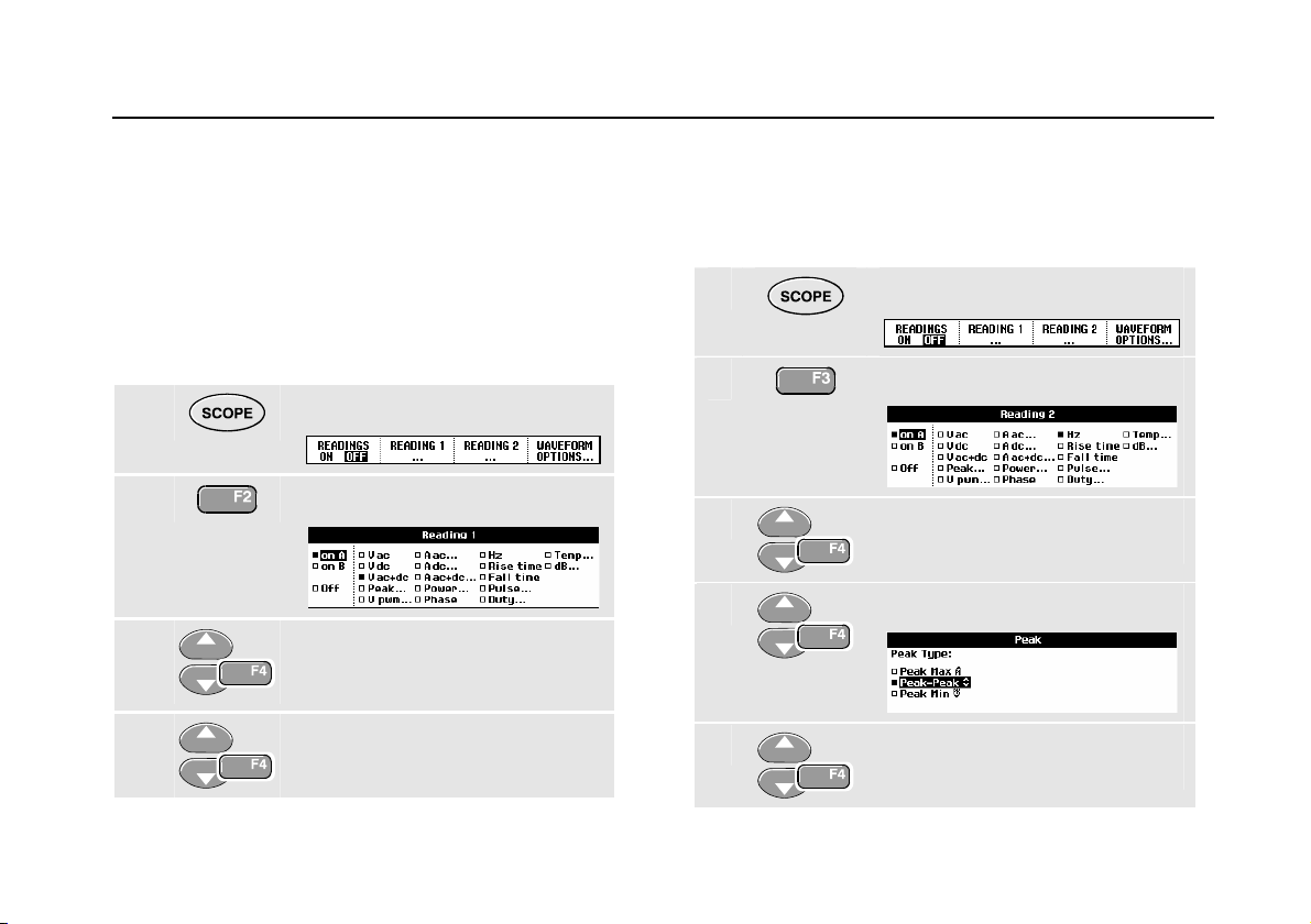
Making Automatic Scope Measurements

The test tool offers a wide range of automatic scope
measurements. You can display two numeric readings:

R

EADING 1 and READING 2. These readings are selectable

independently, and the measurements can be done on the
input A or input B waveform

To choose a frequency measurement for input A, do the
following:

1

2

3

4

Display the SCOPE key labels.

Open the Reading 1 menu.

Select on A. Observe that the
highlight jumps to the present
measurement.

Select the Hz measurement.

Observe that the top left of the screen displays the Hz
measurement. (See Figure 8.)

To choose also a Peak-Peak measurement for Input B as
second reading, do the following:

1

Display the SCOPE key labels.

2

Open the Reading 2 menu.

3

Select on B. The highlight jumps
to the measurements field.

4

Open the PEAK menu.

5

Select the Peak-Peak
measurement.

13

Fluke 19xC-2x5C

Users Manual

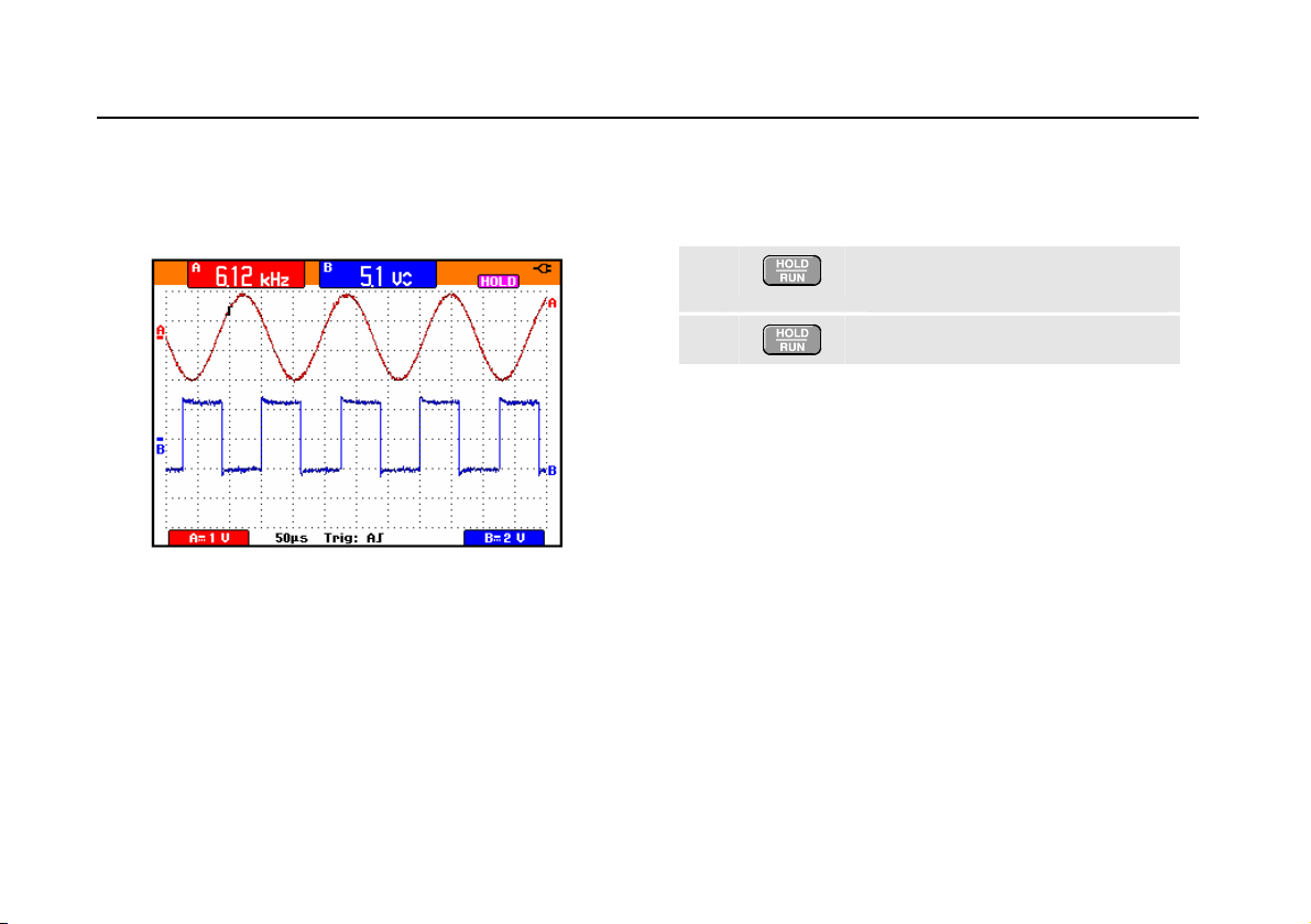
Figure 8 shows an example of the screen. Note that the
Peak-Peak reading for input B appears next to the input A
frequency reading at the top of the screen.

Figure 8. Hz and V peak-peak as Scope Readings

.

Freezing the Screen

You can freeze the screen (all readings and waveforms) at
any time.

1

2

Freeze the screen. HOLD appears
at the right of the reading area.

Resume your measurement.

14

Using The Scope
Using Average, Persistence and Glitch Capture

1

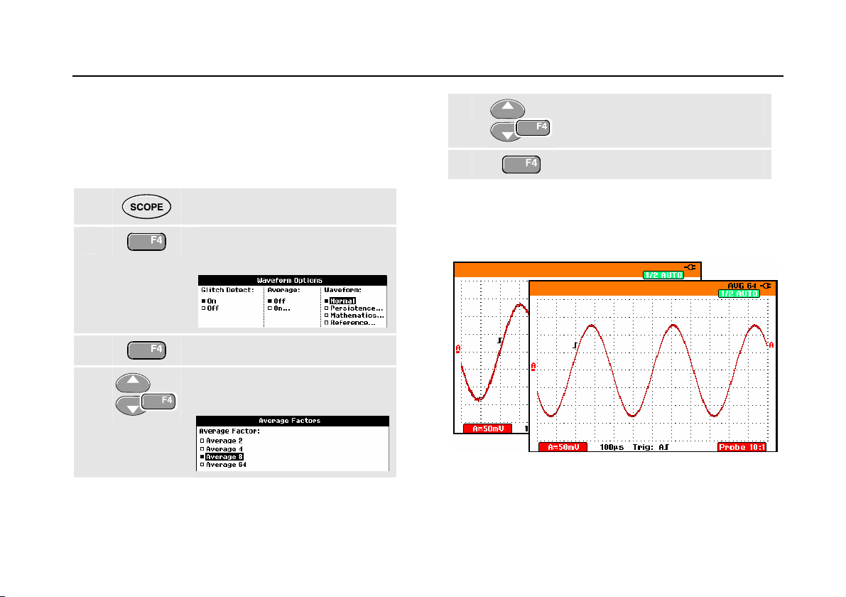
Using Average, Persistence and Glitch Capture

Using Average for Smoothing Waveforms

To smooth the waveform, do the following:

1

2

3

4

Display the SCOPE key labels.

Open the Waveform Options
menu.

Jump to Average:

Select On... to open the Average

Factors menu

5

Select Average 64.This averages
the outcomes of 64 acquisitions.

6

You can use the average functions to suppress random or
uncorrelated noise in the waveform without loss of
bandwidth. Waveform samples with and without smoothing
are shown in Figure 9.

Figure 9. Smoothing a Waveform

Exit the menu.

15

Fluke 19xC-2x5C

Users Manual

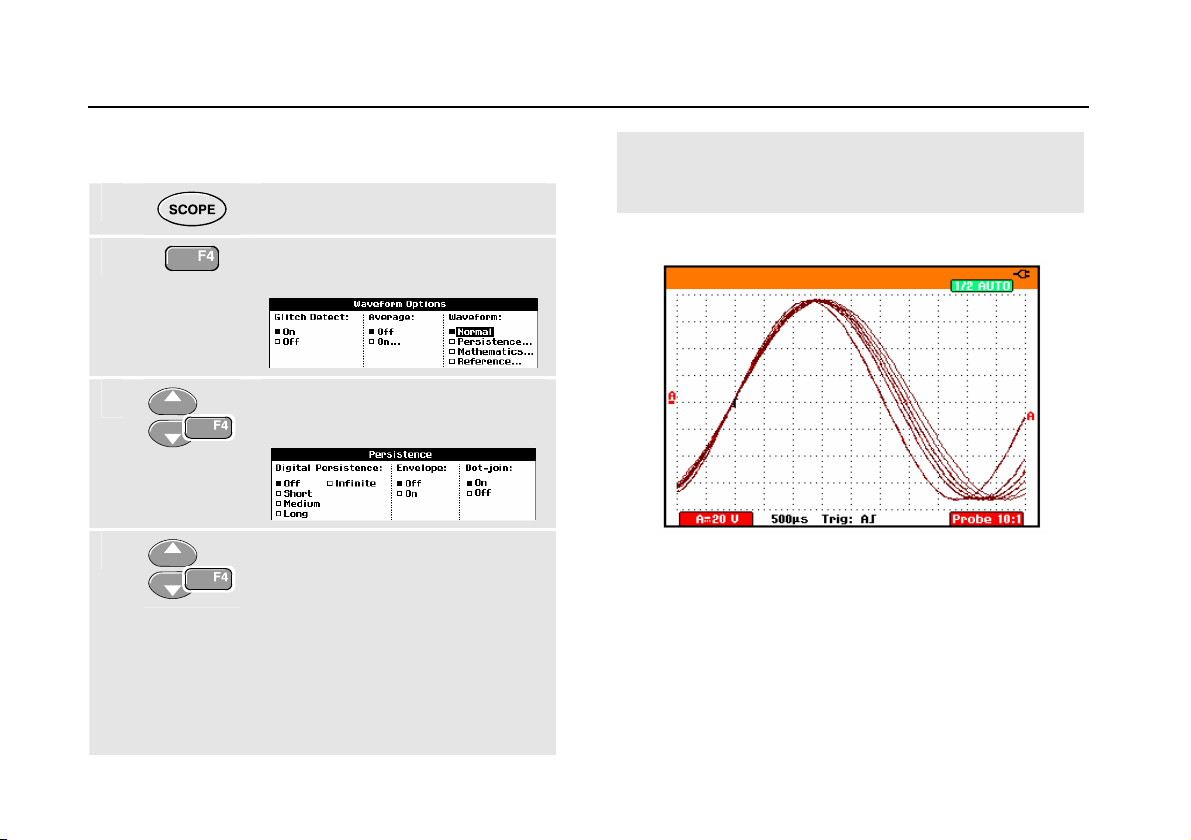
Using Persistence to Display Waveforms

You can use Persistence to observe dynamic signals.

1

Display the SCOPE key labels.

2

3

Open the Waveform Options
menu.

Jump to Waveform: and open the

Persistence... menu.

4

Select Digital Persistence: Short,
Medium, Long or Infinite to

observe dynamic waveforms .

Select Digital Persistence: Off ,
Envelope: On to see the upper
and lower boundaries of dynamic
waveforms (envelope mode).

Select Dot-join: On or Off to
choose your personal preference
for the waveform representation.

Figure 10. Using Persistence to Observe Dynamic

Signals

16

Using The Scope
Using Average, Persistence and Glitch Capture

1

Displaying Glitches

To capture glitches on a waveform, do the following:

1

Display the SCOPE key labels.

2

Open the Waveform Options
menu.

3

Select Glitch Detect: On

4

You can use this function to display events (glitches or
other asynchronous waveforms) of 50 ns (nanoseconds)
or wider, or you can display HF modulated waveforms.

When you select the 2 mV/div range Glitch Detect will be
turned Off. In the 2 mV/div range you can set Glitch Detect
On .

Exit the menu.

Suppressing High Frequency Noise

Switching Glitch Detect to Off will suppress the high
frequency noise on a waveform. Averaging will suppress
the noise even more.

1

Display the SCOPE key labels.

2

3

4

Open the Waveform Options
menu.

Select Glitch Detect: Off, then
select Average: On to open the
Average menu

Select Factor : 8x

Tip

Glitch capture and average do not affect
bandwidth. Further noise suppression is possible
with bandwidth limiting filters. See Chapter 1:
“Working with Noisy Waveforms”.

17

Fluke 19xC-2x5C

Users Manual

Acquiring Waveforms

Selecting AC-Coupling

After a reset, the test tool is dc-coupled so that ac and dc
voltages appear on the screen.

Use ac-coupling when you wish to observe a small ac
signal that rides on a dc signal. To select ac-coupling, do
the following:

1

2

Observe that the bottom left of the screen displays the
ac-coupling icon: .

Display the INPUT A key labels.

Highlight AC.

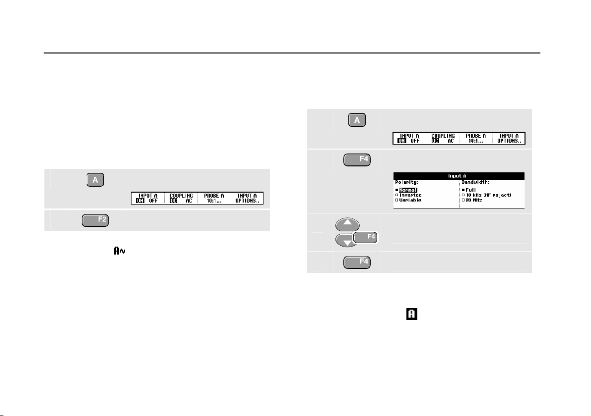
Reversing the Polarity of the Displayed Waveform

To invert the input A waveform, do the following:

1

2

3

Display the INPUT A key labels.

Open the Input A menu.

Select Inverted and accept
inverted waveform display.

4

For example, a negative-going waveform is displayed as
positive-going waveform which may provide a more
meaningful view. An inverted display is identified by an
inversed trace identifier (

Exit the menu.

) at the right of the waveform.

18

Using The Scope
Acquiring Waveforms

1

Variable Input Sensitivity

The variable input sensitivity allows you to adjust the input
A sensitivity continuously, for example to set the amplitude
of a reference signal to exactly 6 divisions.

The input sensitivity of a range can be increased up to 2.5
times, for example between 10 mV/div and 4 mV/div in the
10 mV/div range.

To use the variable input sensitivity, do the following:

1 Apply the input signal

2

An Auto Set will turn off the variable input sensitivity. You
can now select the required input range. Keep in mind
that the sensitivity will increase when you start adjusting
the variable sensitivity (the displayed trace amplitude will
increase).

3

Perform an Auto Set (AUTO must
appear at the top of the screen)

Display the INPUT A key labels.

4

Open the Input A Options...
menu.

5

Select and accept Variable.

6

At the bottom left of the screen the text A Var is
displayed.

Selecting Variable will turn off cursors and automatic input
ranging.

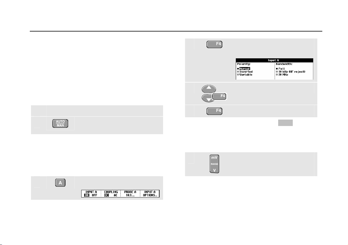
7

Exit the menu.

Press mV to increase the
sensitivity, press V to decrease
the sensitivity.

19

Fluke 19xC-2x5C

Users Manual

Working with Noisy Waveforms

To suppress high frequency noise on waveforms, you can
limit the working bandwidth to 10 kHz or 20 MHz. This
function smoothes the displayed waveform. For the same
reason, it improves triggering on the waveform.

To choose HF reject, do the following:

1

Display the INPUT A key labels.

2

Open the Input A menu.

3

4

Jump to Bandwidth.

Select 10kHz (HF reject) to
accept the bandwidth limitation.

Tip

To suppress noise without loss of bandwidth,
use the average function or turn off Display

Glitches.

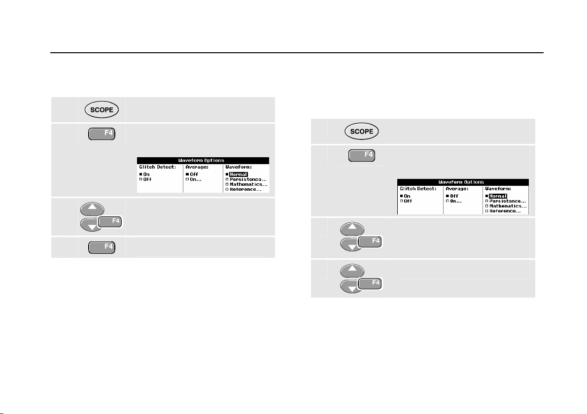
Using Mathematics Functions A±B, AxB, A vs B

When adding (A+B), subtracting (A-B), or multiplying (A*B)
the input A and input B waveform, the test tool will display
the mathematical result waveform and the input A and
input B waveforms.

A versus B provides a plot with input A on the vertical axis
and input B on the horizontal axis.

The Mathematics functions perform a point-to-point
operation on waveforms A and B.

To use a Mathematics function, do the following:

1

Display the SCOPE key labels.

2

Open the Waveform Options
menu.

20

Using The Scope
Acquiring Waveforms

1

3

Jump to Waveform: and Select
Mathematics... to open the
Mathematics menu.

4

Select Function: A+B, A-B, AxB or
A vs B.

5

The sensitivity range of the mathematical result is equal to
the sensitivity range of the least sensitive input divided by
the scale factor.

Select a scale factor to fit the
mathematical result waveform onto
the display, and return.

Using Mathematics Function Spectrum (FFT)

The Spectrum function shows the spectral content of the
input A or input B waveform. It performs an FFT to
transform the amplitude waveform from the time domain
into the frequency domain.

To reduce the effect of side-lobes (leakage) it is
recommended to use auto windowing. It will automatically
adapt the part of the waveform that is analyzed to a
complete number of cycles

Selecting Hanning, Hamming or no windowing results in a
faster update, but also in more leakage.

Ensure that the entire waveform amplitude remains on the
screen.

To use the Spectrum function, do the following:

1

Display the SCOPE key labels.

2

Open the Waveform Options
menu.

21

Fluke 19xC-2x5C

Users Manual

3

Jump to Waveform: and select
Mathematics... to open the
Mathematics menu.

4

Select Function: Spectrum.

5

You will see a screen that looks like Figure 11.

Observe that the top right of the screen displays
SPECTRUM.
If it displays LOW AMPL a spectrum measurement cannot
be done as the waveform amplitude is too low.
If it displays WRONG TB the time base setting does not
enable the test tool to display an FFT result. It is either too
slow, which can result in aliasing, or too fast, which results
in less than one signal period on the screen.

Select Window: Auto (automatic
windowing), Hanning, Hamming,
or None (no windowing).

6

7

8

Perform a spectrum analysis on
trace A, or trace B.

Set the vertical amplitude scale to
linear or logarithmic. The horizontal
frequency scale is always
logarithmic.

Turn the spectrum function off/on
(toggle function).

Figure 11. Spectrum measurement

22

Using The Scope
Acquiring Waveforms

1

Comparing Waveforms

You can display a fixed reference waveform with the
actual waveform for comparison.

To create a reference waveform and to display it with the
actual waveform, do the following:

1

Display the SCOPE key labels.

2

3

4

Open the Waveform Options
menu.

Jump to the Waveform field.

2x

Select Reference… to open the
Waveform Reference menu.

5

Select On to display the reference
waveform. This can be:

- the last used reference waveform
(if not available no reference
waveform will be shown).

- the envelope waveform if the
persistence function Envelope is
on.

Select Recall… to recall a saved
waveform (or waveform envelope)
from memory and use it as a
reference waveform.

Select New… to open the New
Reference menu.

Continue at step 6.

6

Select the width of an additional
envelope to be added to the
momentary waveform.

23

Fluke 19xC-2x5C

Users Manual

7

To recall a saved waveform from memory and use it as a
reference waveform refer also to Chapter 6 Recalling
Screens with Associated Setups.

Example of reference waveform with an additional
envelope of ±2 pixels:

black pixels: basic waveform
gray pixels: ± 2 pixels envelope

1 vertical pixel on the display is 0.04 x range/div
1 horizontal pixel on the display is 0.0375 x range/div

Store the momentary waveform
and display it permanently for
reference. The display also shows
the actual waveform.

Pass - Fail Testing

You can use a reference waveform as a test template for
the actual waveform. If at least one sample of a waveform
is outside the test template, the failed or passed scope
screen will be stored. Up to 100 screens can be stored.
If the memory is full, the first screen will be deleted in favor
of the new screen to be stored.

The most appropriate reference waveform for the
Pass-Fail test is a waveform envelope.

To use the Pass - Fail function using a waveform
envelope, do the following:

1 Display a reference waveform as described in the

previous section “Comparing Waveforms”

2

Each time a scope screen is stored you will hear a beep.
Chapter 4 provides information on how to analyze the
stored screens.

From the Pass Fail Testing: menu
select

Store Fail : each scope screen with
samples outside the reference will
be stored

Store Pass: each scope screen
with no samples outside the
reference will be stored

24

Using The Scope
Analyzing Waveforms

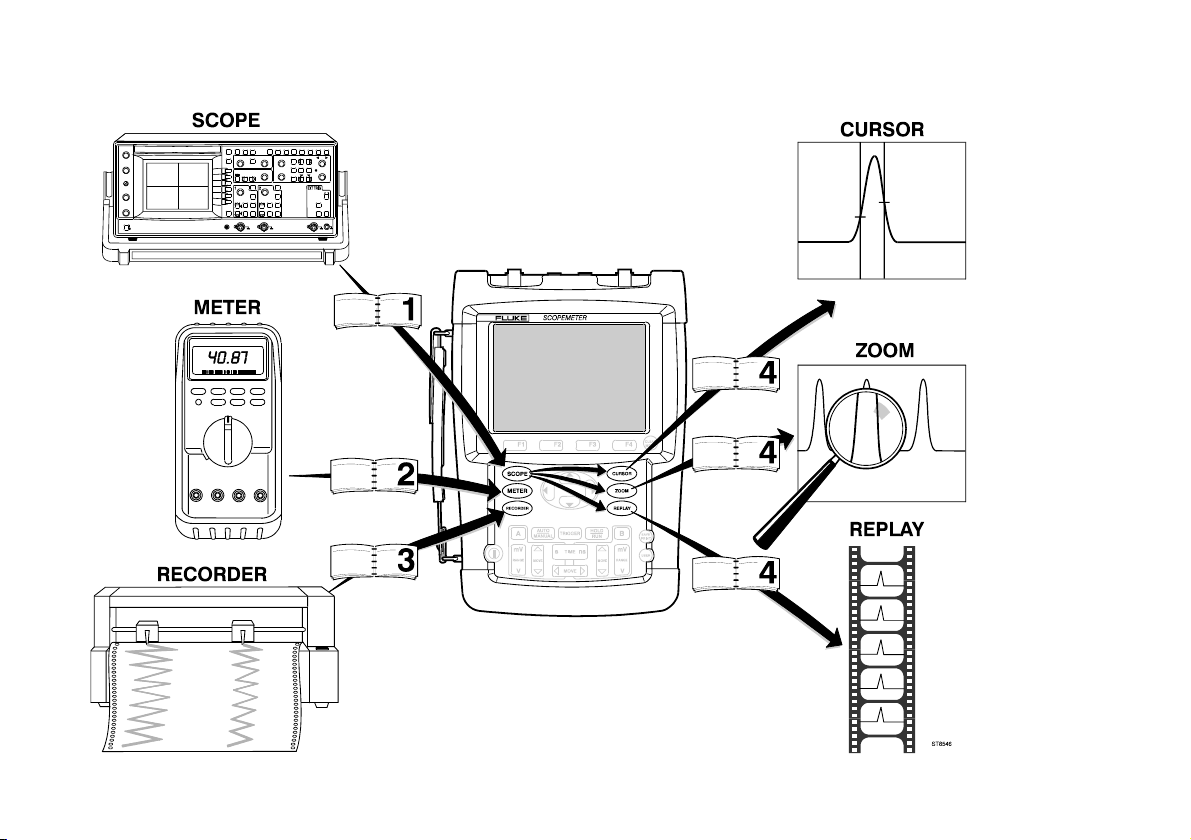
Analyzing Waveforms

You can use the analysis functions CURSOR, ZOOM and

REPLAY to perform detailed waveform analysis. These

functions are described in Chapter 4: “Using Cursors,
Zoom and Replay”.

1

25

Fluke 19xC-2x5C

Users Manual

26

About this Chapter

This chapter provides a step-by-step introduction to the
multimeter functions of the test tool (hereafter called
“meter”). The introduction gives basic examples to show
how to use the menus and perform basic operations.

Chapter 2

Using The Multimeter

Making Meter Connections

Use the two 4-mm safety red ( ) and black (COM)
banana jack inputs for the Meter functions. (See Figure

12.)

Note

Typical use of the Meter test leads and
accessories is shown in Chapter 8.

Figure 12. Meter Connections

27

Fluke 19xC-2x5C

Users Manual

Making Multimeter Measurements

The screen displays the numeric readings of the
measurements on the meter input.

Measuring Resistance Values

To measure a resistance, do the following:

1 Connect the red and black test leads from the

4-mm banana jack inputs to the resistor.

2

3

4

5

Display the METER key labels.

Open the Measurement menu.

Highlight Ohms.

Select Ohms measurement.

The resistor value is displayed in ohms. Observe also that
the bargraph is displayed. (See

Figure 13.)

Figure 13. Resistor Value Readings

28

Using The Multimeter
Making Multimeter Measurements

Making a Current Measurement

You can measure current in both Scope mode and Meter
mode. Scope mode has the advantage of two waveforms
being displayed while you perform measurements.
Meter mode has the advantage of high measurement
resolution.

2

The next example explains a typical current measurement
in Meter mode.

Warning

Carefully read the instructions about the
current probe you are using.

To set up the test tool, do the following:

1 Connect a current probe (e.g. i400, optional)

from the 4-mm banana jack outputs to the
conductor to be measured.

Ensure that the red and black probe connectors
correspond to the red and black banana jack
inputs. (See Figure 14.)

2

Display the METER key labels.

Figure 14. Measurement Setup

3

4

5

Open the Measurement menu.

Highlight A ac....

Open the Current Probe
submenu.

29

Fluke 19xC-2x5C

Users Manual

6

7

Now, you will see a screen like in Figure 15

Observe the sensitivity of the
current probe. Highlight the
corresponding sensitivity in the
menu, e.g. 10 mV/A.

Accept the current measurement.

Figure 15. Ampere Measurement Readings

30

Using The Multimeter
Freezing the Readings

2

Freezing the Readings

You can freeze the displayed readings at any time.

1

2

You can use this function to hold accurate readings for
later examination.

For saving screens into memory, see Chapter 7.

Freeze the screen. HOLD appears
at the top right of the reading
area.

Resume your measurement.

Note

Selecting Auto/Manual Ranges

To activate manual ranging, do the following during any
Meter measurement:

1

2 Increase or decrease the range.

Observe how the bargraph sensitivity changes.

Use manual ranging to set a fixed bargraph sensitivity and
decimal point.

3

When in auto ranging, the bargraph sensitivity and decimal
point are automatically adjusted while checking different
signals.

Activate manual ranging.

Choose auto ranging again.

31

Fluke 19xC-2x5C

Users Manual

Making Relative Measurements

A relative measurement displays the present
measurement result relative to a defined reference value.

The following example shows how to perform a relative
voltage measurement. First obtain a reference value:

1

2

3

This stores the reference value as reference for
subsequent measurements. The stored reference value is
displayed in small digits at the bottom right side of the
screen after the word

4

Display the METER key labels.

Measure a voltage to be used as
reference value.

Set RELATIVE to ON. (ON is
highlighted.)

REFERENCE.

Measure the voltage to be
compared to the reference.

Observe that the main reading is displayed as variations
from the reference value. The actual reading with its
bargraph is displayed beneath these readings. (See Figure

16.)

Figure 16. Making a Relative Measurement

You can use this feature when, for example, you need to
monitor input activity (voltage, resistance, temperature) in
relation to a known good value.

32

About this Chapter

This chapter provides a step-by-step introduction to the
recorder functions of the test tool. The introduction gives
examples to show how to use the menus and perform
basic operations.

Opening the Recorder Main Menu

First choose a measurement in scope or meter mode. Now
you can choose the recorder functions from the recorder
main menu. To open the main menu, do the following:

Chapter 3

Using The Recorder Functions

1

RECORDER

ANALYZE

Open the RECORDER main menu.
(See Figure 17.)

Figure 17. Recorder Main Menu

33

Fluke 19xC-2x5C

A

Users Manual

Plotting Measurements Over Time (TrendPlot™)

Use the TrendPlot function to plot a graph of Scope or
Meter measurements as function of time.

Note

Because the navigations for the dual input
TrendPlot (Scope) and the single input TrendPlot
(Meter) are identical, only TrendPlot (Scope) is
explained in the next sections.

Starting a TrendPlot Function

To start plotting a graph of the reading over time, do the
following:

1 Apply a signal to the red BNC input A and turn

on Reading 1 in scope mode

2

RECORDER

NALYZE

3

4

The test tool continuously records the digital readings of
the input A measurements and displays these as a graph.
The TrendPlot graph rolls from right to left like a paper
chart recorder.

Observe that the recorded time from start appears at the
bottom of the screen. The present reading appears on top
of the screen. (See

When simultaneously TrendPlotting two readings,
the screen area is split into two sections of four
divisions each.

Open the RECORDER main menu.

Highlight Trend Plot (Scope).

Start the TrendPlot recording.

Figure 18.)

Note

34

Using The Recorder Functions
Plotting Measurements Over Time (TrendPlot™)

Displaying Recorded Data

When in normal view (NORMAL), only the twelve most
recently recorded divisions are displayed on screen. All
previous recordings are stored in memory.

VIEW ALL shows all data in memory:

3

7

Press repeatedly to toggle between normal view
(NORMAL) and overview (VIEW ALL)

Display an overview of the full
waveform.

Figure 18. TrendPlot Reading

When the Scope is in automatic mode, automatic vertical
scaling is used to fit the TrendPlot graph on the screen.

5

6

Set RECORDER to STOP to freeze
the recorder function.

Set RECORDER to RUN to restart.

When the recorder memory is full, an automatic
compression algorithm is used to compress all samples
into half of the memory without loss of transients. The
other half of the recorder memory is free again to continue
recording.

35

Fluke 19xC-2x5C

Users Manual

Changing the Recorder Options

At the right bottom of the display you can choose to
display the time elapsed from start and the actual time of
the day.

To change the time reference, proceed from step 6 as
follows:

7

Open the Recorder Options
menu.

8

Select Time of Day or From
Start

Now the recorded time or the current time appear at the
bottom of the screen.

Turning Off the TrendPlot Display

9

Exit the recorder function.

36

Using The Recorder Functions
Recording Scope Waveforms In Deep Memory (Scope Record)

Recording Scope Waveforms In Deep Memory (Scope Record)

The SCOPE RECORD function is a roll mode that logs one or
two long waveforms. This function can be used to monitor
waveforms like motion control signals or the power-on
event of an Uninterruptable Power Supply (UPS). During
recording, fast transients are captured. Because of the
deep memory, recording can be done for more than one
day. This function is similar to the roll mode in many
DSO’s but has deeper memory and better functionality.

Starting a Scope Record Function

1 Apply a signal to the red BNC input A.

2

3

The waveform moves across the screen from right to left
like a normal chart recorder. (See

From the Recorder main menu,
highlight Scope Record.

Start the recording.

Figure 19.)

Observe that the top of the screen displays the following:

• Time from start at the top of the screen.

• The status at the bottom of the screen which includes

Figure 19. Recording Waveforms

the time/div setting as well as the total timespan that
fits the memory.

Note

For accurate recordings it is advised to let the
instrument first warm up for five minutes.

3

37

Fluke 19xC-2x5C

Users Manual

Displaying Recorded Data

In Normal view, the samples that roll off the screen are
stored in deep memory. When the memory is full,
recording continues by shifting the data in memory and
deleting the first samples out of memory.

In View All mode, the complete memory contents are
displayed on the screen.

4

You can analyze the recorded waveforms using the
Cursors and Zoom functions. See Chapter 4: “Using
Replay, Zoom and Cursors”.

Press to toggle between VIEW ALL
(overview of all recorded
samples) and NORMAL view.

Using Scope Record in Single Sweep Mode

Use the recorder Single Sweep function to automatically
stop recording when the deep memory is full.

Continue from step 3 of the previous section:

4

Open the Recorder options
menu.

5

6

Jump to the Mode field

(2x)

Select Single Sweep and accept
the recorder options.

38

Using The Recorder Functions
Recording Scope Waveforms In Deep Memory (Scope Record)

Using External Triggering to Start or Stop Scope Record

To record an electrical event that causes a fault, it might
be useful to start or stop recording on an external trigger
signal:

Start on trigger to start recording; recording stops when
the deep memory is full

Stop on trigger to stop recording.

Stop when untriggered to continue recording as long as

a next trigger comes within 1 division in view all mode.

To set up the test tool, continue from step 3 of the
previous section:

4 Apply the signal to be recorded to the red BNC

input A. Apply a trigger signal to the red and
black external trigger banana inputs. (See Figure

20.)

5

Open the Recorder Options
menu.

Figure 20. Scope Record Using External Triggering

6

7

8

Jump to Display Glitches:.

Jump to Mode:.

Select on EXT. ... to open the

Single Sweep on Ext. menu.

3

39

Fluke 19xC-2x5C

Users Manual

9

Select one of the Conditions:
and jump to Slope:.

10

Select the desired trigger slope,
and jump to Level:

11

During recording samples are continuously saved in deep
memory. The last twelve recorded divisions are displayed
on the screen. Use View All to display the full memory
contents.

To learn more about the Single Shot trigger
function, see Chapter 5 “Triggering on
Waveforms”.

Select the 0.12V or 1.2 V trigger
level and accept all recorder
options.

Note

Figure 21. Triggered Single Sweep Recording

Analyzing a TrendPlot or Scope Record

From a Scope TrendPlot or Scope Record you can use the
analysis functions CURSORS and ZOOM to perform
detailed waveform analysis. These functions are described
in Chapter 4: “Using Replay, Zoom and Cursors”.

40

Using Replay, Zoom and Cursors

About this Chapter

This chapter covers the capabilities of the analysis
functions Cursor, Zoom, and Replay. These functions
can be used with one or more of the primary functions
Scope, TrendPlot or Scope Record.

It is possible to combine two or three analysis functions. A
typical application using these functions follows:

• First replay the last screens to find the screen of

special interest.

• Then zoom in on the signal event.

• Finally, make measurements using the cursors.

Chapter 4

Replaying the 100 Most Recent Scope Screens

When you are in scope mode, the test tool automatically
stores the 100 most recent screens. When you press the

HOLD key or the REPLAY key, the memory contents are

frozen. Use the functions in the REPLAY menu to “go back
in time” by stepping through the stored screens to find the
screen of your interest. This feature lets you capture and
view signals even if you did not press HOLD.

41

Fluke 19xC-2x5C

Users Manual

Replaying Step-by-Step

To step through the last scope screens, do the following:

1

From scope mode, open the

REPLAY menu.

Observe that the trace is frozen
and that REPLAY appears at the
top of the screen (see Figure 22).

2

3

Observe that the bottom of the waveform area displays the
replay bar with a screen number and related time stamp:

Step through the previous
screens.

Step through the next screens.

42

Figure 22. Replaying a Waveform

The replay bar represents all 100 stored screens in
memory. The icon represents the picture being
displayed on the screen (in this example: SCREEN -84). If
the bar is partly white, the memory is not completely filled
with 100 screens.

From this point you can use the zoom and cursor functions
to study the signal in more detail.

Using Replay, Zoom and Cursors
Replaying the 100 Most Recent Scope Screens

4

Replaying Continuously

You can also replay the stored screens continuously, like
playing a video tape.

To replay continuously, do the following:

1

From Scope mode, open the

REPLAY menu.

Observe that the trace is frozen
and REPLAY appears at the top of
the screen.

2

Wait until the screen with the signal event of interest
appears.

3

Continuously replay the stored
screens in ascending order.

Stop the continuous replay.

Turning Off the Replay Function

4

Turn off REPLAY.

Capturing 100 Intermittents Automatically

When you use the test tool in triggered mode, 100
triggered screens are captured. This way you could use
Pulse Triggering to trigger and capture 100 intermittent
glitches or you could use External Triggering to capture
100 UPS startups.

By combining the trigger possibilities with the capability of
capturing 100 screens for later replay, you can leave the
test tool unattended to capture intermittent signal
anomalies.

For triggering, see Chapter 5: “Triggering on Waveforms”.

43

Fluke 19xC-2x5C

Users Manual

Zooming in on a Waveform

To obtain a more detailed view of a waveform, you can
zoom in on a waveform using the

To zoom in on a waveform, do the following:

ZOOM function.

1

Display the ZOOM key labels.

Observe that the trace is frozen,

ZOOM appears at the top of the

screen, and the waveform is
magnified.

2

3

Enlarge (decrease the time/div) or
shrink (increase the time/div) the
waveform.

Scroll. A position bar displays the
position of the zoomed part in
relation to the total waveform.

Tip

Even when the key labels are not displayed at the
bottom of the screen, you can still use the arrow
keys to zoom in and out.

44

Figure 23. Zooming in a Waveform

Observe that the bottom of the waveform area displays the
zoom ratio, position bar, and time/div (see
zoom range depends on the amount of data samples
stored in memory.

From this point you can use the cursor function for further
measurements on the waveform.

Figure 23). The

Using Replay, Zoom and Cursors
Zooming in on a Waveform

4

Displaying the Zoomed Waveform

The VIEW ALL feature is useful when you quickly need to
see the complete waveform and then return to the zoomed
part.

4

Press repeatedly to toggle between the zoomed part
of the waveform and the complete waveform.

Display the complete waveform.

Turning Off the Zoom Function

5

Turn off the ZOOM function.

45

Fluke 19xC-2x5C

Users Manual

Making Cursor Measurements

Cursors allow you to make precise digital measurements
on waveforms. This can be done on live waveforms,
recorded waveforms, and on saved waveforms.

Using Horizontal Cursors on a Waveform

To use the cursors for a voltage measurement, do the
following:

1

2

3

4

5

6

From scope mode, display the
cursor key labels.

Press to highlight . Observe
that two horizontal cursors are
displayed.

Highlight the upper cursor.

Move the upper cursor to the
desired position on the screen.

Highlight the lower cursor.

Move the lower cursor to the
desired position on the screen.

Note

Even when the key labels are not displayed at the
bottom of the screen, you still can use the arrow
keys. This allows full control of both cursors while
having full screen view.

Figure 24. Voltage Measurement with Cursors

The screen shows the voltage difference between the two
cursors and the voltage at the cursors. (See

Use horizontal cursors to measure the amplitude, high or
low value, or overshoot of a waveform.

Figure 24.)

46

Using Replay, Zoom and Cursors
Making Cursor Measurements

Using Vertical Cursors on a Waveform

To use the cursors for a time measurement, or for an RMS
measurement of the trace section between the cursors (C
versions), do the following:

4

1

From scope mode, display the
cursor key labels.

2

3

4

5

6

7

47

Press to highlight . Observe
that two vertical cursors are
displayed. Markers (—) identify the
point where the cursors cross the
waveform.

Choose for example time
measurement: READING T.

If necessary, choose the trace:

TRACE A ,B, or M (Mathematics).

Highlight the left cursor.

Move the left cursor to the desired
position on the waveform.

Highlight the right cursor.

Figure 25. Time Measurement with Cursors

8

The screen shows the time difference between the cursors
and the voltage difference between the two markers. (See
Figure 25.)

9

Move the right cursor to the
desired position on the waveform.

Select OFF to turn off the cursors.

Fluke 19xC-2x5C

Users Manual

Using Cursors on a A+B, A-B or A*B Waveform

Cursor measurements on a A*B waveform give a reading
in Watts if input A measures (milli)Volts and input B
measures (milli)Amperes.

For other cursor measurements on a A+B, A-B or A*B
waveform no reading will be available if the input A and
input B measurement unit are different.

Using Cursors on Spectrum Measurements

To do a cursor measurent on a spectrum, do the following:

1

From Spectrum measurement
display the cursor key label.

2

Move the cursor and observe the
readings at the top of the screen.

48

Using Replay, Zoom and Cursors
Making Cursor Measurements

4

Making Rise Time Measurements

To measure rise time, do the following:

1

2

3

4

From scope mode, display the
cursor key labels.

Press to highlight (rise time).
Observe that two horizontal
cursors are displayed.

For multiple traces select the
required trace A, B, or M (if a
math function is active).

Select MANUAL or AUTO (this
automatically does steps 5 to 7).

5

6

Move the upper cursor to 100% of
the trace height. A marker is
shown at 90%.

Highlight the other cursor.

7

The reading shows the risetime from 10%-90% of the
trace amplitude.

Move the lower cursor to 0% of
the trace height. A marker is
shown at 10%.

Figure 26. Risetime Measurement

49

Fluke 19xC-2x5C

Users Manual

50

About this Chapter

This chapter provides an introduction to the trigger
functions of the test tool. Triggering tells the test tool when
to begin displaying the waveform. You can use fully
automatic triggering, take control of one or more main
trigger functions (semi-automatic triggering), or you can
use dedicated trigger functions to capture special
waveforms.

Following are some typical trigger applications:

• Use the Connect-and-View™ function to have full

automatic triggering and instant display of virtually any
waveform.

Chapter 5

Triggering on Waveforms

• If the signal is unstable or has a very low frequency,

you can control the trigger level, slope, and trigger
delay for a better view of the signal. (See next
section.)

• For dedicated applications, use one of the four

manual trigger functions:

• Edge triggering

• External triggering

• Video triggering

• Pulse Width triggering

51

Fluke 19xC-2x5C

Users Manual

Setting Trigger Level and Slope

The Connect-and-View™ function enables hands-off
triggering to display complex unknown signals.

When your test tool is in manual range, do the following:

Automatic triggering assures a stable display of virtually
any signal.

From this point, you can take over the basic trigger
controls such as level, slope and delay. To optimize trigger
level and slope manually, do the following:

1

2

Perform an auto set. AUTO appears
at the top right of the screen.

Display the TRIGGER key labels.

Trigger on either positive slope or
negative slope of the chosen
waveform.

Dual Slope Triggering ( X ):

19xC-2x5C versions can trigger on
both positive slope and negative
slope.

3

Enable the arrow keys for manual
trigger level adjustment.

Figure 27. Screen with all Trigger Information

4

Observe the trigger icon that indicates the trigger
position, trigger level, and slope.

At the bottom of the screen the trigger parameters are
displayed (See Error! Reference source not found.) .
For example,
the trigger source with a positive slope.

When no trigger is found, the trigger parameters appear in
gray.

Adjust the trigger level.

means that input A is used as

52

Triggering on Waveforms
Using Trigger Delay or Pre-trigger

Using Trigger Delay or Pre-trigger

You can begin to display the waveform some time before
or after the trigger point has been detected. Initially, you
have 2 divisions of pre-trigger view (negative delay).

To set the trigger delay, do the following:

5

5

Observe that the trigger icon on the screen moves to
show the new trigger position. When the trigger position
moves left off of the screen, the trigger icon changes into

to indicate that you have selected a trigger delay.
Moving the trigger icon to the right on the display gives
you a pre-trigger view.

In case of a trigger delay, the status at the bottom of the
screen will change. For example:

This means that input A is used as the trigger source with
a positive slope. The 500.0 ms indicates the (positive)
delay between trigger point and waveform display.

When no trigger is found, the trigger parameters appear in
gray.

Hold down to adjust the trigger
delay.

Figure 28. Trigger Delay or Pre-trigger View

Figure 28 shows an example of a trigger delay of 500 ms
(top) and an example of pre-trigger view of 8 divisions
(bottom).

53

Fluke 19xC-2x5C

Users Manual

Automatic Trigger Options

In the trigger menu, settings for automatic triggering can
be changed as follows. (See also Chapter 1: “Displaying
an Unknown Signal with Connect-and-View”)

1

The

TRIGGER key labels can differ depending on

the latest trigger function used.

2

3

Display the TRIGGER key labels.

Note

Open the Trigger Options menu.

Open the Automatic Trigger menu.

If the frequency range of the automatic triggering is set to
> 15 Hz, the Connect-and-View™ function responds more
quickly. The response is quicker because the test tool is
instructed not to analyze low frequency signal
components. However, when you measure frequencies
lower than 15 Hz, the test tool must be instructed to
analyze low frequency components for automatic
triggering:

4

Select > 1 HZ and return to the
measurement screen.

54

Triggering on Waveforms
Triggering on Edges

5

Triggering on Edges

If the signal is instable or has a very low frequency, use
edge triggering to obtain full manual trigger control.

To trigger on rising edges of the input A waveform, do the
following:

1

2

3

When Free Run is selected, the test tool updates the
screen even if there are no triggers. A trace always
appears on the screen.

Display the TRIGGER key labels.

Open the Trigger Options menu.

Open the Trigger on Edge menu.

When On Trigger is selected, the test tool needs a trigger
to display a waveform. Use this mode if you want to
update the screen only when valid triggers occur.

When Single Shot is selected, the test tool waits for a
trigger. After receiving a trigger, the waveform is displayed
and the instruments is set to HOLD.

In most cases it is advised to use the Free Run mode:

4

Select Free Run, jump to Noise
reject Filter.

5

Set Noise reject Filter to Off.

6

Set NCycle to Off

Observe that the key labels at the bottom of the screen
have adapted to allow further selection of specific edge
trigger settings:

55

Fluke 19xC-2x5C

Users Manual

Triggering on Noisy Waveforms

To reduce jitter on the screen when triggering on noisy
waveforms, you can use a noise rejection filter. Continue
from step 3 of the previous example as follows:

4

Select On Trigger, jump to Noise
reject Filter.

5

Set Noise reject Filter to On.

Observe that the trigger gap has increased. This is
indicated by a taller trigger icon .

Making a Single Acquisition

To catch single events, you can perform a single shot
acquisition (one-time screen update). To set up the test
tool for a single shot of the input A waveform, continue
from step 3 again:

4

Select Single Shot.

5

Accept the settings.

The word WAITING appears at the top of the screen
indicating that the test tool is waiting for a trigger. As soon
as the test tool receives a trigger, the waveform is
displayed and the instrument is set to hold. This is
indicated by the word HOLD at top of the screen.

The test tool will now have a screen like

6

Arm the test tool for a new single
shot.

Figure 29.

Tip

The test tool stores all single shots in the replay
memory. Use the Replay function to look at all
the stored single shots.

Figure 29. Making a Single Shot Measurement

56

Triggering on Waveforms
Triggering on Edges

5

N-Cycle Triggering

N-Cycle triggering enables you to create a stable picture of
for example n-cycle burst waveforms.

Each next trigger is generated after the waveform has
crossed the trigger level N times in the direction that
complies with the selected trigger slope.

To select N-Cycle triggering, continue from step 3 again:

4

Select On Trigger or Single Shot,
jump to Noise reject Filter.

5

Set Noise reject Filter On or Off.

6

Set NCycle to On

Observe that the key labels at the bottom of the screen
have been changed to allow further selection of specific
N-Cycle trigger settings:

7

Set the number of cycles N

8 Adjust the trigger level

Traces with N-Cycle triggering (N=2) and without N-Cycle
triggering are shown in Figure 30.

Figure 30. N-Cycle triggering

57

Fluke 19xC-2x5C

Users Manual

Triggering on External Waveforms

Use external triggering when you want to display
waveforms on inputs A and B while triggering on a third
signal. You can choose external triggering with automatic
triggering or with edge triggering.

1 Supply a signal to the red and black 4-mm

banana jack inputs. See Figure 31.

In this example you continue from the Trigger on Edges
example. To choose the external signal as trigger source,
continue as follows:

Figure 31. External Triggering

2

3

Observe that the key labels at the bottom of the screen
have been adapted to allow selection of two different
external trigger levels: 0.12 V and 1.2 V:

Display the TRIGGER (On Edges)
key labels.

Select Ext (external) edge trigger.

58

4

From this point the trigger level is fixed and is compatible
with logic signals.

Select 1.2V under the Ext LEVEL
label.

Triggering on Waveforms
Triggering on Video Signals

Triggering on Video Signals

To trigger on a video signal, first select the standard of the
video signal you are going to measure:

1 Apply a video signal to the red input A.

5

2

Display the TRIGGER key labels.

3

Open the Trigger Options menu.

Figure 32. Measuring Interlaced Video Signals

4

Select Video on A … to open the
Trigger on Video menu.

6

Select the video standard and
return.

Trigger level and slope are now fixed.

Observe that the key labels at the bottom of the screen

5

59

Select positive signal polarity for
video signals with negative going
sync pulses.

have been changed to allow further selection of specific
video trigger settings:

Fluke 19xC-2x5C

Users Manual

Triggering on Video Frames

Use FIELD 1 or FIELD 2 to trigger either on the first half of
the frame (odd) or on the second half of the frame
(even).To trigger on the second half of the frame, do the
following:

7

The signal part of the even field is displayed on the
screen.

Choose FIELD 2.

Triggering on Video Lines

Use ALL LINES to trigger on all line synchronization
pulses (horizontal synchronization).

7

The signal of one line is displayed on the screen. The
screen is updated with the signal of the next line
immediately after the test tool triggers on the horizontal
synchronization pulse.

To view a specific video line in more detail, you can select
the line number. For example, to measure on video line
123, continue from step 6 as follows:

7

8

The signal of line 123 is displayed on the screen. Observe
that the status line now also shows the selected line
number. The screen is continuously updated with the
signal of line 123.

Choose ALL LINES.

Enable video line selection.

Select number 123.

60

Triggering on Waveforms
Triggering on Pulses

5

Triggering on Pulses

Use pulse width triggering to isolate and display specific
pulses that you can qualify by time, such as glitches,
missing pulses, bursts or signal dropouts.

Detecting Narrow Pulses

To set the test tool to trigger on narrow positive pulses
shorter than 5 ms, do the following:

1 Apply a video signal to the red input A.

2

3

Display the TRIGGER key labels.

Open the Trigger Options menu.

4

Select Pulse Width on A... to
open the Trigger on Pulse Width
menu.

5

Select the positive pulse icon,
then jump to Condition.

6

Select <t, then jump to Update.

7

Select On Trigger.

The test tool is now prepared to trigger on narrow pulses
only. Observe that the trigger key labels at the bottom of
the screen have been adapted to set the pulse conditions:

61

Fluke 19xC-2x5C

Users Manual

To set the pulse width to 5 ms, do the following:

7

8

All narrow positive pulses shorter than 5 ms are now
displayed on the screen. (See Figure 33.)

Enable the arrow keys to adjust
the pulse width.

Select 5 ms.

Tip

The test tool stores all triggered screens in the
replay memory. For example, if you setup your
triggering for glitches, you can capture 100
glitches with time stamps. Use the REPLAY key to
look at all the stored glitches.

Figure 33. Triggering on Narrow Glitches

62

Triggering on Waveforms
Triggering on Pulses

5

Finding Missing Pulses

The next example covers finding missing pulses in a train
of positive pulses. In this example it is assumed that the
pulses have a 100 ms distance between the rising edges.
If the time accidently increases to 200 ms, a pulse is
missing. To set the test tool to trigger on such missing
pulses, let it trigger on gaps bigger than about 150 ms.
Do the following:

1

Display the TRIGGER key labels.

2

Open the Trigger Options menu.

3

Select Pulse Width on A... to
open the Trigger on Pulse Width
menu.

4

5

Select the positive pulse icon to
trigger on the gap between the
positive pulses, then jump to
Condition.

Select >t, then jump to Update.

6

The test tool is now prepared to trigger on pulse gaps.
Observe that the trigger menu at the bottom of the screen
has been adapted to set the pulse condition:

Select On Trigger.

63

Fluke 19xC-2x5C

Users Manual

To set the pulse width to 150 ms, continue as follows:

7

8

Enable the arrow keys to adjust
the pulse width.

Select 150 ms.

Figure 34. Triggering on Missing Pulses

64

Chapter 6

Using The Bushealth Function

About this Chapter

This chapter provides a step-by-step introduction to the
Bushealth function of the test tool. For extended
information on Fieldbuses and fieldbus measurement
please consult Appendix A of this manual.

Bushealth Function Availability

The Bushealth function is available in the models
Fluke 215C and Fluke 225C.

Introduction

Fieldbuses are bi-directional, digital, serial control
networks used in process control and industrial
automation.

The test tool bushealth function indicates the status of the
following aspects of the OSI model Physical Layer:

• Voltage levels (bias, high level, low level)

• Bit width – baud rate

• Rise and fall time

• Distortion

Moreover the test tool can show the bus signal waveform
in the Eye-pattern mode, see

Figure 46.

65

Fluke 19xC-2x5C

A

Users Manual

The bushealth measurement is based upon the test tool
Scope mode. The test tool selects settings that are
optimized to the signal characteristics of the selected bus
type. It operates in full automatic (ranging and triggering)
mode.

Test limits are preset, but can be changed, see page

For supported bus types and protocols see Chapter 10,
Specifications, section ‘Fieldbus Measurements’.

Note

You can perform resistance measurements using
the Meter mode to check a suspected cable or
bus termination.

81.

Performing Bushealth Measurements

Caution

Fieldbuses often are controlling delicate
processes that must not be disturbed. It is
strongly recommended to contact the system
manager before any connections are made!

Selecting the bus type

To select the fieldbus type do the following:

1

2 Highlight Bushealth.

3

NALYZE

4 Select the bus type.

Open the bushealth/fieldbus main
selection screen.

Open the Select Fieldbus
menu:

66

Using The Bushealth Function
Performing Bushealth Measurements

6

5

The test tool starts measuring now. You will see a screen
like

Figure 35.

Each bus type has a default probe setting (e.g. 10:1). If the
probe setting before selecting the fieldbus type was
different from this default probe setting, the probe menu is
shown with the default setting highlighted. To accept the

default setting press
probe type now using the arrow keys.

6 Connect the inputs as indicated in section Input

Connections and Tested Signals on page 70

Press
on measurement connections.

Accept your choice.

For bus types followed by 3 dots
… a new menu will open:

Select the required item and

press .

. You can also select another

Tip

(WIRING INFO) to get information

Starting and Stopping Measuring

Measuring starts immediately after you selected a bus
type. The test tool now continuously monitors the bus
signal and shows the signal properties. Measured
minimum and maximum values (the extremes) will be
stored and displayed from now on. To clear these values
you can stop and start measuring as follows:

1

2

Press to stop measuring. The
screen is frozen now. Press again
to start a new measurement

Press to clear the screen and
start measuring again.

Selecting a probe type

To select another probe type, do the following:

1

2

3

Select the input A or B key labels.

Open the Probe On A (B) menu

Select and accept ( ) the
required probe attenuation.

67

Fluke 19xC-2x5C

A

Users Manual

Reading the Screen

The bus test screen (see the example Figure 35 ) shows
the status of the various signal properties.

Information is represented in five columns:

A. signal property that is being tested, for example

V-Level Bias. See page

tested signal properties for each bus.

B. status indicator, for example . See Table 1 for a

description of the indicators.

C. most recent measurement value, for example 3.5.

--- indicates that no reading is available

OL indicates that the signal is out of the

measurement range (overload)

D. Min Max : the lowest and highest measured value

E. Limit: used low (left) and high (right) test limits, for

example 18.5 31.6V.

LIMIT * the * indicates that one or more of the

limits are not set to the default value!

N/A indicates that limit does Not Apply to this

bus type.

The F1…F4 function key labels are explained in

70 for a description of the

Table 2.

B C D E

Figure 35. Field Bus Test Screen Example

68

Using The Bushealth Function

MAXMI

N

Reading the Screen

6

Table 1. Bus Test Screen Indicators

Bus activity indicator 1:

Q (filled) : voltage measured

{ (open) : no voltage measured

Bus activity indicators 2 and 3:
{ { (both open) : no activity

: bus activity indicators.

ÑÑ(blinking) : activity

Busy, the test tool is measuring/processing
data.

No reading available.

Test OK. Measurement results are within 80%
of allowable range, see

Warning. Measurement results are between
80% and 100% of allowable range, see
36

Test failed. Measurement results are out of
allowable range, see

Figure 36.

Figure

Figure 36.

Figure 36 shows the bus health indicator boundaries.

WEAK WEAK BADBAD

Figure 36. Bus Health Indicator Boundaries

Example:

the high level voltage of a bus must be between +3.0 V
(MIN) and +15.0 V (MAX). Depending on the
measurement result the displayed indicator will be:

If the result is between 4.2 and 13.8V. (10% of
12 V = 1.2 V)

If the result is between 3 V and 4.2 V, or between

13.8 V and 15 V.

If the result is < 3 V or >15 V.

GOOD

80 %10 % 10 %

69

Fluke 19xC-2x5C

Users Manual

Table 2. F1...F4 Key Functions

Select the Limit Setup function, see page

81.

Shows how to connect the test tool to the
bus.

Select the Eye-pattern screen mode, see
Viewing the Bus Waveform Screen on
page 79.

Turn fieldbus test function ON/OFF.

Input Connections and Tested Signals

This section provides a short description of the required
bus connection and the measured signal properties.

See Appendix A for detailed information.

For correct measurements you should calibrate your
probe to match its characteristics to the test tool. A
poorly calibrated probe can introduce measurement
errors. See Chapter 9, section ‘Calibrating the Voltage
Probes’ for calibration instructions.

Data Traffic

In some bus systems (AS-i for instance) the protocol uses
continuous polling of all devices in a fixed time schedule
so that there is continuous data traffic. Other systems
such as RS-232 only carry data when communication is
required. Bushealth requires continuous data traffic to
perform its measurements. In case of very low data
repetition rates, the banner ‘NO DATA’ is displayed. In
systems with low data rates, it is recommended to
increase the data rate by e.g. knob operation. Contact the
system manager for this.

70

Using The Bushealth Function
Input Connections and Tested Signals

6

AS-i Bus

Default probe setting 10:1. Use the Fluke 10:1 probe.

1 Connect the red probe to test tool input A

2 Connect the probe ground lead to the AS-i bus -

3 Connect the probe tip to the AS-i bus +

AS-i +
AS-i -

Figure 37. AS-i Bus Measurement Connections

Table 3. AS-i Bus Tested Signal Properties

Signal Description

V-Level Bias Bias voltage
V-Level Peak-Peak voltage

Note

The bus normally has continuous data traffic.

71

Fluke 19xC-2x5C

Users Manual

CAN Bus

Default probe setting 10:1. Use the Fluke 10:1 probes.

1 Connect the red probe to the test tool input A,

connect the grey probe to input B.

2 Connect the ground lead of the input A probe to

the CAN bus High (CAN_H)

3 Connect the probe tip of the input A probe to the

CAN bus Low (CAN_L)

4 Connect the ground lead of the input B probe to

the CAN bus ground (CAN_GND)

5 Connect the probe tip of the input B probe to the

CAN bus high (CAN_H)

Note

The bus normally has continuous data traffic.

CAN-H

CAN-GND

CAN-L

Figure 38. CAN Bus Measurement Connections

Table 4. CAN Bus Tested Signal Properties

Signal Description

CAN Dom. H-L Dominant high to low level voltage
CAN Rec. H-L Recessive high to low level voltage
CAN-Level Common mode voltage
Data Bit width
Rise Rise time as % of bit width
Fall Fall time as % of bit width
Jitter Jitter distortion
Overshoot Overshoot distortion

72

Using The Bushealth Function

TxD

D

Input Connections and Tested Signals

6

RS-232 Bus & Modbus IEA-232/RS-232

Default probe setting 10:1. Use the Fluke 10:1 probe.

1 Connect the red probe to the test tool input A.

2 Connect the probe ground lead to the RS-232

bus Signal Ground.

3 Connect the probe tip to the RS-232 bus TxD or

RxD.

or Rx

GND

Figure 39. RS-232 Bus Measurement Connections

Table 5. RS-232 Bus Tested Signal Properties

Signal Description

V-Level High High level voltage
V-Level Low Low level voltage
Data Bit width
Rise Rise time as % of bit width
Fall Fall time as % of bit width
Jitter Jitter distortion
Overshoot Overshoot distortion

Note

Continuous data traffic is not ensured . See
Traffic on page 70

Data

73

Fluke 19xC-2x5C

DATA

Users Manual

RS-485 Bus & MOD Bus IEA-485/RS-485

Default probe setting 10:1. Use the Fluke 10:1 probes.

1 Connect the red probe to the test tool input A

and the grey probe to input B.

2 Connect the ground lead of the input A probe to

the RS-485 bus RxD/TxD N (-)

3 Connect the ground lead of the input B probe to

the RS-485 bus cable shield.

4 Connect the probe tip of both probes to the

RS-485 bus RxD/TxD P (+)

+

DATA -

DATA GND

Figure 40. RS-485 Bus Measurement Connections

Table 6. RS-485 Bus Tested Signal Properties

Signal Description

V-Offset High level voltage
V-Level Peak-peak voltage
Data Bit width
Rise Rise time as % of bit width
Fall Fall time as % of bit width
Jitter Jitter distortion
Signal Dist.

Overshoot

Signal distortion (Manchester
decoding, default setting)
Overshoot (NRZ decoding, can be
selected via limit setup)

Note

Continuous data traffic is not ensured . See

Data

Traffic on page 70

74

Using The Bushealth Function
Input Connections and Tested Signals

6

Foundation H1 Bus

Default probe setting 10:1. Use the Fluke 10:1 probe.

1 Connect the red probe to test tool input A

2 Connect the probe ground lead to the H1 bus +

3 Connect the probe tip to the H1 bus -

DATA +

DATA -

Figure 41. Foundation H1 Bus Measurement

Connections

Table 7. Foundation H1 Bus Tested Signal Properties

Signal Description

V-Level Bias Bias voltage level
V-Level Peak-peak voltage
Data Bit width
Rise Rise time as % of bit width
Fall Fall time as % of bit width
Jitter Jitter distortion
Signal Dist. Signal distortion
Noise-HF High Frequency noise >39.1 kHz
Noise Mid Frequency noise 7.8 ….39.1 kHz
Noise-LF Low Frequency noise < 7.8 kHz

The bus normally has continuous data traffic.

Note

75

Fluke 19xC-2x5C

Users Manual

Profibus PA/31.25 kBit/s

Default probe setting 10:1. Use the Fluke 10:1 probe.

1 Connect the red probe to test tool input A

2 Connect the probe ground lead to the PA bus -

3 Connect the probe tip to the PA bus +

DATA +

DATA -

Figure 42. Profibus PA Measurement Connections

Warning

Profibus PA is optimized for process control
with focus on explosion safety.

When planning tests on this bus type, make
sure the proper safety rules are adhered to!

Table 8. Profibus PA Tested Signal Properties

Signal Description

V-Level Bias Bias voltage level
V-Level Peak-peak voltage
Data Bit width
Rise Rise time as % of bit width
Fall Fall time as % of bit width
Jitter Jitter distortion
Signal Dist. Signal distortion
Noise-HF High Frequency noise >39.1 kHz
Noise Mid Frequency noise 7.8 -39.1 kHz
Noise-LF Low Frequency noise < 7.8 kHz

Note

The bus normally has continuous data traffic.

76

Using The Bushealth Function

DATA

Input Connections and Tested Signals

6

Profibus DP/RS-485

Default probe setting 10:1. Use the Fluke 10:1 probes.

1 Connect the red probe to the test tool input A

and the grey probe to input B.

2 Connect the ground lead of the input A probe to

the DP bus RxD/TxD N (-)

3 Connect the ground lead of the input B probe to

the DP bus cable shield.

4 Connect the probe tip of both probes to the DP

bus RxD/TxD P (+)

+

DATA -

DATA GND

Figure 43. Profibus DP Measurement Connections

Table 9. Profibus DP Tested Signal Properties

Signal Description

V-Offset

V-Level Peak-peak voltage
Data Bit width
Rise Rise time as % of bit width
Fall Fall time as % of bit width
Jitter Jitter distortion
Signal Dist.

Overshoot

The bus normally has continuous data traffic.

V offset

Signal distortion (Manchester
decoding, default setting)
Overshoot (NRZ decoding, can be
selected via limit setup)

Note

77

Fluke 19xC-2x5C

Eth

Users Manual

Ethernet Coax/10Base2

Default probe setting 1:1. Use the Fluke 1:1 probes.

1 Connect a male BNC to dual female BNC

adapter (Fluke PM9093) to input A.

2 Connect the Ethernet bus as shown below,

using an additional coax cable.

Caution

The Ethernet cabling may be interrupted for
onlly a few seconds during normal process
operation!

ernet coax

Ethernet coax

PM9093

Figure 44. Ethernet Bus Measurement Connections

Table 10. Ethernet Coax Bus Tested Signal Properties

Signal Description

V-Level High Voltage level high
V-Level Low Voltage level low
Data Bit width
Rise Rise time as % of bit width
Fall Fall time as % of bit width
Jitter Jitter distortion
Signal Dist. Signal distortion

Note

Normally the Ethernet bus has continuous data
traffic. Incidentally the bus may have no
continuous data traffic. See

Data Traffic on page

70.

78

Using The Bushealth Function
Input Connections and Tested Signals

6

Ethernet Twisted Pair/10BaseT/100BaseT

Default probe setting 10:1. Use the Fluke 10:1 probe.

1 Connect the red probe to test tool input A

2 Connect the probe ground lead to the bus TD+

(RD+)

3 Connect the probe tip to the bus TD- (RD-)

TD+ (RD+)
TD- (RD-)

Figure 45. Ethernet Twisted Pair Measurement

Connections

Note

Normally the Ethernet bus has continuous data
traffic. Incidentally the bus may have no
continuous data traffic. See

70.

Data Traffic on page

Table 11. Ethernet Twisted Pair Tested Signal

Properties

Signal Description

V-Level Peak-Peak voltage
Data Bit width
Rise Rise time as % of bit width
Fall Fall time as % of bit width
Jitter Jitter distortion
Signal Dist. Signal distortion

79

Fluke 19xC-2x5C

Users Manual

Viewing the Bus Waveform Screen

To view the waveform eye pattern of the bus voltage, do
the following:

1

The screen shows the waveforms of one bit time triggered
on a positive as well as on a negative edge in persistence
mode.

2

3

4

In the main screen select eye
pattern mode. You will see a
screen like Figure 46.

Clear the persisted waveforms
and restart showing the
waveform.

Open the Persistence menu.

Select Digital Persistence:
Short, Medium, Long or Infinite
to observe dynamic waveforms .

Select Dot-join: On or Off to
choose your personal preference
for the waveform representation.

Return to the test screen.

5

Figure 46. Eye Pattern Screen

- Press

again will clear the persistence waveform

and restart showing the waveform eye pattern.

Exit the Bushealth mode and
enter the Scope/Meter mode.

Notes

to freeze the screen. Pressing

80

Using The Bushealth Function
Setting the Test Limits

6

- When saving a screen the most recently

acquired waveform will be stored. Persistence
waveforms will not be stored.

Setting the Test Limits

You can change the test limits used to generate the
messages OK , WARNING , and NOT OK .

The test limits apply to the selected bus type. To select a
bus type do steps 1-5 on page

To change the test limits of the selected bus, do the
following:

1

From the bus test screen open
the SETUP LIMITS menu. You
will see a screen like Figure 47.

The header does not show the
bus type. To see the bus type
when you are changing the limits
press the CLEAR MENU key.
Press this key again to return to
the setup limits screen.

66.

2 Select the signal property for

which you want to set the limit.

3

4

5

Select the level to be adjusted:
LOW (low level), HIGH (high
level) or WARNING ! (warning
level)

Change the limits.

A * before a line in the SETUP
LIMITS screen indicates that a
signal property in that line has
limits that differ from the default
setting.

Press N/A if a limit should
not be involved in the test.

Press DEFAULTS to set
all limits to the default values.

Accept the limits and return to the
test screen.

In the test screen the word LIMIT
will be followed by a * if any of the
limits has not the default value.

81

Fluke 19xC-2x5C

Users Manual

Note

Changed limits will persist until:

- you change them again,

- you reset the test tool; resetting will restore the
default limits.

Figure 47. Setup Limits Menu Screen

Saving and Recalling Test Limits

You can save a screen, plus the test setup with (adjusted)
test limits, plus the most recent eye pattern trace as a new
dataset. By recalling this dataset you can do a bus test
according to your own pre-defined test limits.

Refer to chapter 7 ‘Saving and Recalling Datasets’.

82

Chapter 7

Using Memory, PC and Printer

About this Chapter

This chapter provides a step-by-step introduction to the
general functions of the test tool that can be used in the
three main modes: Scope, Meter, or Recorder. You will
find information on printer and computer communication at
the end of this chapter.

Saving and Recalling

You can:

• Save screens and setups to memory, and recall them

again from memory. The test tool has 15 ‘screen and
setup’ memories and 2 ‘record and setup’ memories.

• Name saved screens and setups according to your

own preferences.

• Recall screens and recordings to analyze or print the

screen image at a later date.

• Recall a setup to continue a measurement with the

recalled operating configuration.

83

Fluke 19xC-2x5C

Users Manual

Saving Screens with Associated Setups

To save for example a screen+setup in Scope mode, do
the following:

1

From this point the screen is frozen until you hide the

SAVE/PRINT key labels again.

2

3

Display the SAVE/PRINT key labels.

Open the Save menu.

Observe the number of available
and used memory locations.

In METER mode the Edit Name
menu will be shown now as only a
setup+screen can be saved.

Highlight Screen+Setup .

4

Open the Edit Name menu. This
menu enables you to name the
saved screen+setup (Save as: )

If no free memory locations are available a message pops
up that proposes to you to overwrite the oldest data set.

Do one of the following:

If you don’t want to overwrite the oldest data set,

- press , then delete one or more memory

locations, and save again.

If you want to overwrite the oldest data set,

- press and continue at step 4.

To name the screen+setup according to your own
preferences, do the following:

5

Skip to a new character position.

84

Using Memory, PC and Printer
Saving and Recalling

7

6

7

To use the default name generated by the test tool,
continue from step 4 as follows:

5

6

The two record+setup memory locations store more than
what is just visible on the screen. In TrendPlot or scope
record mode the full recording is saved. In scope mode
you can save all 100 replay screens in a single
record+setup memory location. The table below shows
what you can store for the various test tool modes.

To save a Trendplot press STOP first.

Select another character.

Repeat 5 and 6 until done.

Save the actual screen.

Use default name.

Save the actual screen.

Notes

Mode Memory locations

15x ‘screen+setup’ 2x ‘record+setup’

METER setup+1screen N/A

SCOPE setup+1screen setup+100 replay screens

SCOPE REC setup setup+record data

TRENDPLOT setup setup+trendplot data

BUSHEALTH setup+1 screen *) N/A

*) in eye pattern mode and persistence mode the most
recently written trace will be saved, not all persistence
traces.

Deleting Screens with Associated Setups

To delete a screen and associated setup, do the following:

1

Display the SAVE/PRINT key labels.

2

3

4

Open the View/Delete menu.

Highlight a screen+setup

Delete the saved screen+setup.

85

Fluke 19xC-2x5C

Users Manual

Recalling Screens with Associated Setups

To recall a screen+setup, do the following:

1

Display the SAVE/PRINT key labels.

2

3

4

Observe that the recalled waveform is displayed and that

HOLD appears on the screen. From this point you can use

cursors and zoom for analysis or you can print the recalled
screen.

To recall a screen as a reference waveform to compare it
with an actually measured waveform, continue from step 3
as follows:

4

5

Open the Recall menu.

Highlight a screen+setup.

Recall the saved screen+setup.

Use RECALL FOR REFERENCE to
recall the saved screen.

Resume the measurement. Both,
the reference screen and the
measurement screen will be
displayed.

Recalling a Setup Configuration

To recall a setup configuration, do the following:

1

2

3

4

Observe that RUN appears at the top right of the screen.
From this point you continue in the new operating
configuration.

Display the SAVE/PRINT key labels.

Open the Recall menu.

Highlight a screen+setup.

Recall the saved setup.

86

Using Memory, PC and Printer
Saving and Recalling

7

Viewing Stored Screens

To scroll through the memories while looking at the stored
screens, do the following:

1

Display the SAVE/PRINT key labels.

2

3

4

5

6

The replay stores (max. 2) cannot be viewed!

Open the View/Delete menu.

Highlight a screen+setup location..

View the screen, and open the
viewer.

Scroll through all stored screens.

Exit the View mode.

Note:

Renaming Stored Screens

To modify the name of stored screens, do the following:

1

Display the SAVE/PRINT key labels.

2

3

4

5

6 Select another character.

7

To select a default name generated by the test tool,
continue from step 4 as follows:

5

6

Open the View/Delete menu.

Highlight a screen+setup location.

Open the Rename menu.

Skip to a new character position.

Repeat 5 and 6 until done.

Save the new name.

Generate the default name.

Save the new name.

87

Fluke 19xC-2x5C

Users Manual

Documenting Screens

With the FlukeView® software you can upload waveform
data and screen bitmaps to your PC or notebook computer
for further processing. Printing can also be done by
connecting the test tool directly to a printer.

Connecting to a Computer

To connect the test tool to a PC or notebook computer and
use the FlukeView software for Windows® (SW90W), do
the following:

z Use the Optically Isolated Adapter/Cable (USB:

OC4USB; RS-232: PM9080) to connect a computer to
the OPTICAL PORT of the test tool. (See

Figure 48. Connecting a Computer

Figure 48.)

Note

For information about installing and using the
FlukeView ScopeMeter software, see the
SW90W Users Manual.

A Software & Cable Carrying Case Kit is optionally
available as model number SCC190.

Connecting to a Printer

To print a screen directly to a printer, use one of the
following adapters:

z The Optically Isolated RS-232 Adapter/Cable

(PM9080, optional) to connect a serial printer to the
OPTICAL PORT of the test tool. (See

z The Print Adapter Cable (PAC91, optional) to connect

a parallel printer to the OPTICAL PORT of the test
tool. (See

Before printing, you must setup the test tool for a specific
printer.

Figure 50.)

Figure 49.)

88

Using Memory, PC and Printer
Documenting Screens

7

Setting up the Printing Configuration

This example demonstrates how to set up the test tool for
printing on a postscript printer with a 9600 baud rate:

1

Display the USER OPTIONS key
labels.

Figure 49. Connecting a Serial Printer

2

Open the User Options menu.

3

Open the Printer Setup submenu.

4

Figure 50. Connecting a Parallel Printer

5

Select Postscript and jump to
Baud Rate.

Select a baud rate of 9600 and
return to normal mode.

89

Fluke 19xC-2x5C

Users Manual

Whenever possible, choose the option Postscript when
printing screens. This option gives the best printing results.
Consult the manual that came with your printer to find out
whether it has Postscript printing possibilities.

To connect the SII (Seiko Instruments Inc.) DPU-414
thermal printer you must use the printer adapter cable
PAC91. (See

Figure 50)

Printing a Screen

To print the currently displayed screen, do the following:

1

2

3

A message appears at the bottom of the screen indicating
that the test tool is busy printing.

Screens will be printed in black and white.

Clear the menu if you do not want
to print it.

Display the SAVE/PRINT key labels.

Start printing.

90