FLIR A6700sc, A6750sc, A6650, A6600 User Manual

A6700sc/A6750sc

User’s Manual

This document is controlled to FLIR Technology Level 2. The information contained in this document pertains to a dual use product controlled for export by the Export Administration Regulations (EAR). Diversion contrary to US law is prohibited. US Department of Commerce authorization is not required prior to export or transfer to foreign persons or parties unless otherwise prohibited.

Document Number: 29249-000 Version: 5 Issue Date: February 2, 2015

FLIR Systems, Inc.

9 Townsend West, Nashua, NH 03063

Support: 1-800-GO-INFR A (800-464-6372)

http://flir.custhelp.com

A6700sc/A6750sc User’s Manual

Service: 1-866-FLIR-911

www.flir.com

Table of Contents

1 REVISION HISTORY ...................................................................................................................................... 6

2 INTRODUCTION ............................................................................................................................................. 7

2.1 Camera System Components .......................................................................................... 7

2.2 System Overview............................................................................................................. 7

2.3 Key features of the A6700sc/A6750sc cameras .............................................................. 8

3 WARNINGS AND CAUTIONS ...................................................................................................................... 10

4 INSTALLATION ............................................................................................................................................ 11

4.1 Basic Connections ......................................................................................................... 11

4.1.1 Power ......................................................................................................................................... 12

4.1.2 Analog Video .............................................................................................................................. 12

4.1.3 GigE Digital Vi deo ...................................................................................................................... 12

5 CAMERA CONTROLLER ............................................................................................................................. 13

5.1 ResearchIR Mini Controller ............................................................................................ 13

5.1.1 Single Preset Mode .................................................................................................................... 13

5.1.2 Superframing Mode [A675xsc only] ........................................................................................... 13

5.2 Menu Bar ....................................................................................................................... 14

5.2.1 Tools Menu ................................................................................................................................. 14

Advanced Time Controls .................................................................................................................................... 14

5.2.2 Help Menu .................................................................................................................................. 15

5.2.3 Status Page ................................................................................................................................ 15

5.2.4 Setup Page ................................................................................................................................. 16

5.2.4.1 Setup Tab ................................................................................................................................... 16

5.2.4.2 Sync Tab [A6750sc only] ............................................................................................................ 17

5.2.4.2.1 Sync Mode .......................................................................................................................................... 17

5.2.4.2.2 Sync Source ........................................................................................................................................ 20

5.2.4.2.3 Sync Options ....................................................................................................................................... 21

5.2.4.2.4 Sync Out ............................................................................................................................................. 22

5.2.5 Correction Page .......................................................................................................................... 22

NUC Information ................................................................................................................................................. 24

Manage NUCs .................................................................................................................................................... 24

Load NUC Options .............................................................................................................................................. 24

Performing a NUC .............................................................................................................................................. 25

What is a Non-Uniformity Correction (NUC)? ..................................................................................................... 27

5.2.5.1.1 One-Point Correction Process............................................................................................................. 28

5.2.5.1.2 Two-Point Correction Process............................................................................................................. 28

A6700sc/A6750sc User’s Manual

5.2.5.1.3 Offset Update ...................................................................................................................................... 29

5.2.5.1.4 Bad Pixel Correction ........................................................................................................................... 29

5.2.6 Video Page ................................................................................................................................. 31

6 INTERFACES ................................................................................................................................................ 34

6.1 Mechanical (dimensions in inches) ................................................................................ 34

6.1.1 Status Lights ............................................................................................................................... 36

6.1.2 Power Interface .......................................................................................................................... 36

6.1.3 Other Interfaces .......................................................................................................................... 37

6.1.3.1 Gigabit Ethernet .......................................................................................................................... 37

6.1.3.2 Sync In ........................................................................................................................................ 37

6.1.3.3 Video .......................................................................................................................................... 37

6.1.3.4 AUX Connector [A6750sc only] .................................................................................................. 37

7 SPECIFICATIONS ........................................................................................................................................ 39

7.1 Interface ........................................................................................................................ 39

7.2 Windowing Capacity ...................................................................................................... 39

7.3 Acquisition Modes and Features .................................................................................... 39

7.4 Analog Video ................................................................................................................. 40

7.5 Performance Characteristics ......................................................................................... 40

7.6 Non Uniformity Correction ............................................................................................. 41

7.7 Detector/FPA ................................................................................................................. 41

7.8 General Characteristics ................................................................................................. 42

8 MAINTENANCE ............................................................................................................................................ 43

8.1 Camera and Lens Cleaning ........................................................................................... 43

8.1.1 Camera Body, Cables and Accessories ..................................................................................... 43

8.1.2 Lenses ........................................................................................................................................ 43

9 INFRARED PRIMER ..................................................................................................................................... 45

9.1 History of Infrared .......................................................................................................... 45

9.2 Theory of Thermography ............................................................................................... 48

9.2.1 Introduction ................................................................................................................................. 48

9.2.2 The Electromagnetic Spectrum .................................................................................................. 48

9.2.3 Blackbody Radiation ................................................................................................................... 48

Planck’s Law ....................................................................................................................................................... 49

Wien’s Displacement Law ................................................................................................................................... 50

Stefan-Boltzmann's Law ..................................................................................................................................... 51

Non-Blackbody Emitters ..................................................................................................................................... 52

9.2.4 Infrared Semi-Transparent Materials .......................................................................................... 54

9.3 The Measurement Formula ........................................................................................... 55

9.4 Emissivity tables ............................................................................................................ 58

A6700sc/A6750sc User’s Manual

1 Revision History

Version

Date

Initials

Changes

08/27/13

Added 2D drawings, corrections

1 08/26/13 RM Initial Release

3 11/21/13 RM Corrections to specifications section 4 11/05/14 RM Removed ITAR control statement. 5 02/02/15 RM Added A6750sc GigE

1 – Revision History

A6700sc/A6750sc User’s Manual

2 – Introduction

2 Introduction

2.1 Camera System Components

The A6700sc infrared camera and its accessories are delivered in a box which typically contains the items below. There may also be additional items that you have ordered such as lenses, software, CDs, etc.

Description FLIR Part Number A67xxsc Camera 29350-2xx Power supply, 24V, 4A 24123-000 AC line cord 24124-000 Gigabit Ethernet Cat-6 cable, 2m length 23700-000 Bayonet mount plug 23901-000 BNC cable 26393-000 ResearchIR Max download/activation card T199013 AUX connector breakout cable [A6750sc only] 29402-500 Laboratory calibration plate 261-0005-00 Water-resistant transit case 24043-000 Documentation CD 24048-050

2.2 System Overview

The A6700sc infrared camera system has been developed by FLIR Advanced Thermal Solutions (ATS) to meet the needs of the commercial R&D user. The camera makes use of FLIR’s advanced ISC0403 4-channel readout integrated circuit (ROIC), mated to an Indium Antimonide (InSb) detector to cover the midwave infrared band. The A6700sc camera utilizes a large format, 640 x 512 array with 15μm pixel pitch.

The A6700sc is a stand-alone imaging camera that interfaces to host PC using Gigabit Ethernet. An SDK is available, which makes it possible for t he system designer to write their own camera cont roller and acquire image data with their own custom application.

A6700sc/A6750sc User’s Manual

2.3 Key features of the A6700sc/A6750sc cameras

Fully GEV/GenICam compliant

The image stream protocol is GigE Vision 2.0 compliant and the camera is fully controllable by GenICam.

Improved Linearity to Zero Well-Fill

Typical direct injection ROIC designs exhibit a non-linear response when the signal drops below 10% of well-fill. The ISC0403 ROIC provides a linear response even at very low signal levels. This results in an increased linear dynamic range, much better NUC performance at low signal levels and makes it easier to perform a user calibration of the camera.

14-Bit Digital Image Data

The A6700sc camera system is built around high performance 14-bit A/D converters, preserving the full dynamic range of the FPA.

Windowing Capability

Higher frame rates are available by windowing down at the Focal Plane Array (FPA) level. The A6700sc has three available window sizes with a max frame rate of 480Hz. The A6750sc has flexible window sizes with frame rates up to 4kHz.

2 – Introduction

Presets

Up to four presets and their associated parameters such as integration time, frame rate, window size and window location, are available for instant selection with a single command.

Superframing [A6750sc only]

Up to four presets can be cycled continuously. This can be used in conjunction with the Dynamic Range Extension (DRX) algorithm to provide a single movie with increased dynamic range.

Independently Adjustable Frame Rates

Frame rate is user selectable from 0.0015 Hz up to the maximum allowed for the select ed window size.

External Sync

The A6700sc camera provides a SYNC input that can be used to control the camera frame rate using an external LVCMOS input (can handle 5.5V Max) .

External Trigger [A6750sc only]

An external trigger input can be used to signal ResearchIR to start rec ording or to precisely start the image stream relative to an external event.

Multiple Video Outputs

The A6700sc camera features multiple independent and simultaneous video:

▫ Digital – Gigabit Ethernet ▫ Analog – Composite video (NTSC or PAL)

Analog Video Color Palettes

The A6700sc camera supports a selection of standard and user-defined color palettes f or th e analog video output.

A6700sc/A6750sc User’s Manual

2 – Introduction

Digital Detail Enhancement (DDE)

DDE is an analog video AGC mode that provides a significant improvement to scene detail

and contrast.

On-Camera NUCs with Auto Update

NUCs can be stored in camera memory and can be applied independently to the digital and

analog video outputs. The camera can be configured to automatically update the NUC using the internal flag based on a change of an internal temperature sensor and/or a timer.

Standard Lens Interface

The A6700sc camera uses th e same bayonet-mount as other SCx000 series cameras. However, even though the mount is the same, due to differences in the opto-mechanical layout, lenses for the SC6000/4000 are not an optimal solution for the A6700sc. The SC6000 lenses will provide fairly good imagery but some vignetting in the corners may be visible. For best performance the user should use lenses designed for the A6700sc. Lenses for the SC8000 will not work on the A6700sc.

A6700sc/A6750sc User’s Manual

3 – Warnings and Cautions

3 Warnings and Cautions

For best results and user safety, the following warnings and precautions should be followed when handling and operating the camera.

Warnings and Cautions:

 Do not open the camera body for any reason. Disassembly of the camera (including

removal of the cover) can cause permanent damage and will void the warranty.

 Great care should be exercised with your camera optics. Refer to Chapter 7 for lens

cleaning.

 Operating the camera outside of the specified input voltage range or the specified

operating temperature range can cause permanent damage.

 The camera is not completely sealed. Avoid exposure to dust and moisture and replace

the lens cap when not in use.

 Do not image extremely high intensity radiation sources, such as the sun, lasers, arc

welders, etc.

 The camera is a precision optical instrument and should not be exposed to excessive

shock and/or vibration. Refer to the Chapter 6 for detailed environmental requirements.

 The camera contains static-sensitive electronics and should be handled appropriately.

A6700sc/A6750sc User’s Manual

4 Installation

4.1 Basic Connections

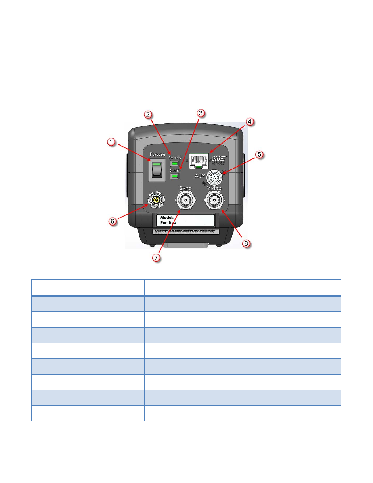
All connections to the A6700sc are located on the Back Panel.

4 – Installation

Item Name Description

1 2 3 4 5 6 7 8

Power Switch LED will light when power is ON

Ready Light LED will turn on when camera is booted

Cold LED LED will light when FPA temp is <80K

Gigabit Ethernet (RJ45) Connect to a PC for digital IR image data

AUX Connector A675xsc only. (See Section 6.1.3.4 for details) DC Power Input 24VDC

Sync Input External Frame Sync

Video Out NTSC or PAL, selectable in camera controller

A6700sc/A6750sc User’s Manual

4 – Installation

4.1.1 Power

Plug in the AC power supply to a standard 120V outlet. Connect the DC power cable between the power supply and the power connector located on the rear panel of the A6700sc camera. Turn on the imaging head by pressing the power button on the rear panel. The green power LED will illuminate to indicate that the unit is ON.

4.1.2 Analog Video

The camera will automatically boot up into the last saved state. The boot process takes about 30 seconds. To see the Composite video on a monitor, connect the provided BNC cable from the VIDEO port to your monitor. If you are powering up the camera for the first time, the camera should produce a 640x480 image with Non-Unifority Correction (NUC), ba d pixel replacement enabled.

4.1.3 GigE Digital Video

If you have a PC data system running ResearchIR (or your own custom application based on the BHP SDK) you can view the 14-bit digital video over Gigabit Ethernet.

The A6700sc has a Gigabit Ethernet interface that is GigE Vision (GEV) and GenICam compliant Use a regular CAT5e or CAT6 Ethernet patch cable. If a crossover cable is used, the camera interface will automatically detect and configure itself to work with this kind of cable.

A6700sc/A6750sc User’s Manual

5 –Camera Controller

5 Camera Controller

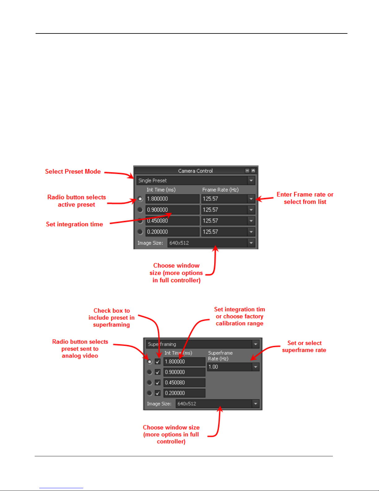
5.1 ResearchIR Mini Controller

The Camera Controller (also called the Graphical User Interface or GUI) can be accessed from within the ResearchIR software. Once you are connected to the camera, a mini controller will be visible in the left pane. This controller will have basic controls for the most commonly used settings, like integration time, frame rate, preset selection, and window size. Choosing the Camera>>Control menu option will display the full camera controller. The rest of this chapter will describe the full camera controller features in detail.

5.1.1 Single Preset Mode

5.1.2 Superframing Mode [A675xsc only]

A6700sc/A6750sc User’s Manual

5.2 Menu Bar

The menu bar is the same for both Basic and Advanced User Modes .

Saves the camera state to the current (name). This

Save State (name)

Save State As

Load State Load a state from flash memory. Manage States Rename or delete states from camera memory.

state will be reloaded at power up. Stored in flash memory.

Saves the current camera state to a name chosen by the user. State names other than (name) my be loaded manually. Stored in flash memory

5 –Camera Controller

Load Factory Defaults

Loads factory defaults for all camera Settings and NUCs. The factory defaults cannot be modified by the user.

NOTE: Camera states contain information about all configurable camera parameters. They do not contain the NUC data, but contain the filenames of the currently loaded NUCs. These NUCs will be reloaded with the state, however, if the NUCs are changed, deleted, or renamed, the state may not be able to load the NUCs.

5.2.1 Tools Menu

Set Camera Time to

PC Time

NOTE: The A6700sc has two internal clocks: a Real Time Clock (RTC) and a timestamp clock. The RTC is a low

resolution clock used to keep system time. The RTC has a battery backup and will retain time while the camera is off. The timestamp clock is a high resolution clock (1us). This clock does not have a battery backup but at power up the timestamp clock is initialized to the current RTC time and will free-wheel until the camera is power cycled.

Advanced…

Sets the camera RTC clock to the time from the PC clock.

Allows user to manually set the IRIG and RTC clocks in the camera. See Section

4.2.2.1

Advanced Time Controls

This dialog is accessed using the Tools>>Set Time>>Advanced menu options. This allows the user to directly set the cameras system time. The Get button will pull time from the PC clock. The Set button will set the camera RTC clock using the manually entered time.

A6700sc/A6750sc User’s Manual

5 –Camera Controller

Figure 4-1 Advanced Time Controls

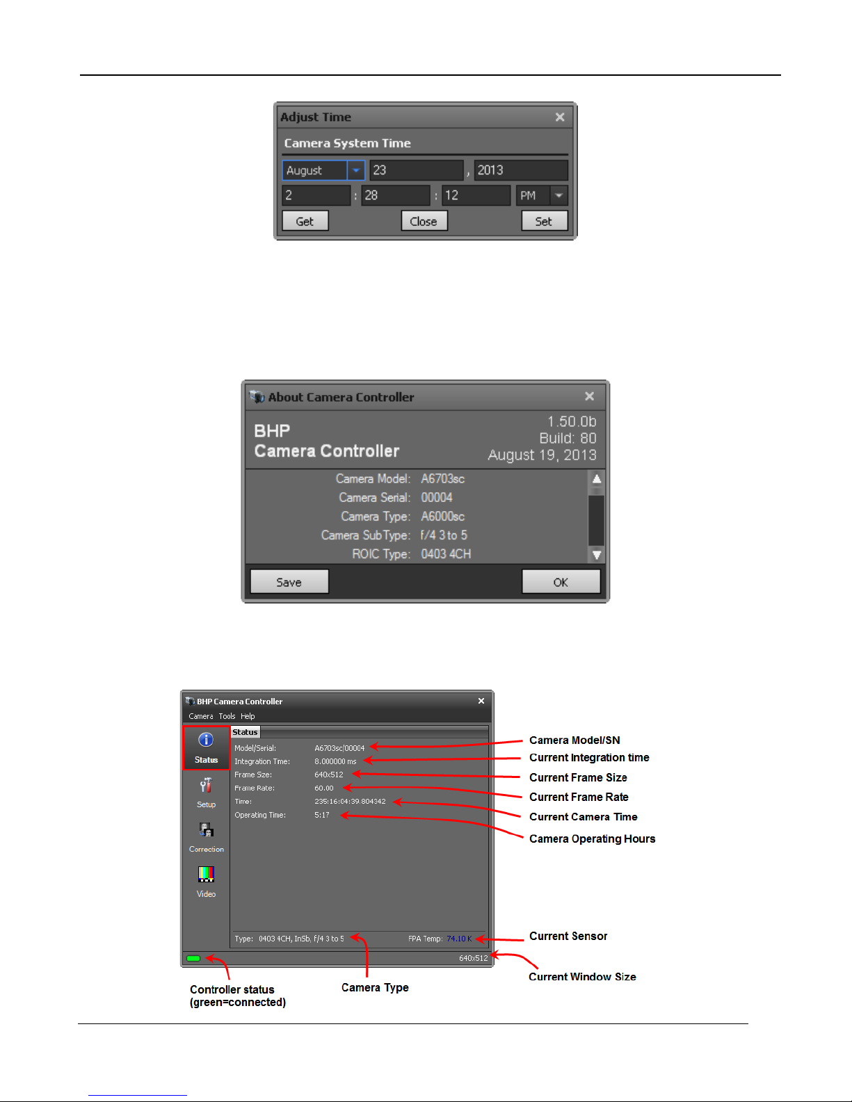
5.2.2 Help Menu

The “About” menu item shows a dialog indicating the current controller version number. If the controller is connected to a camera a list will be displayed that shows all versions of software and firmware in the camera. The “Save” button allows the user to create a text file with this version information.

5.2.3 Status Page

The Status Page gives general information about the camera state including camera type, camera time, integration time, frame size, and frame rate.

A6700sc/A6750sc User’s Manual

5 –Camera Controller

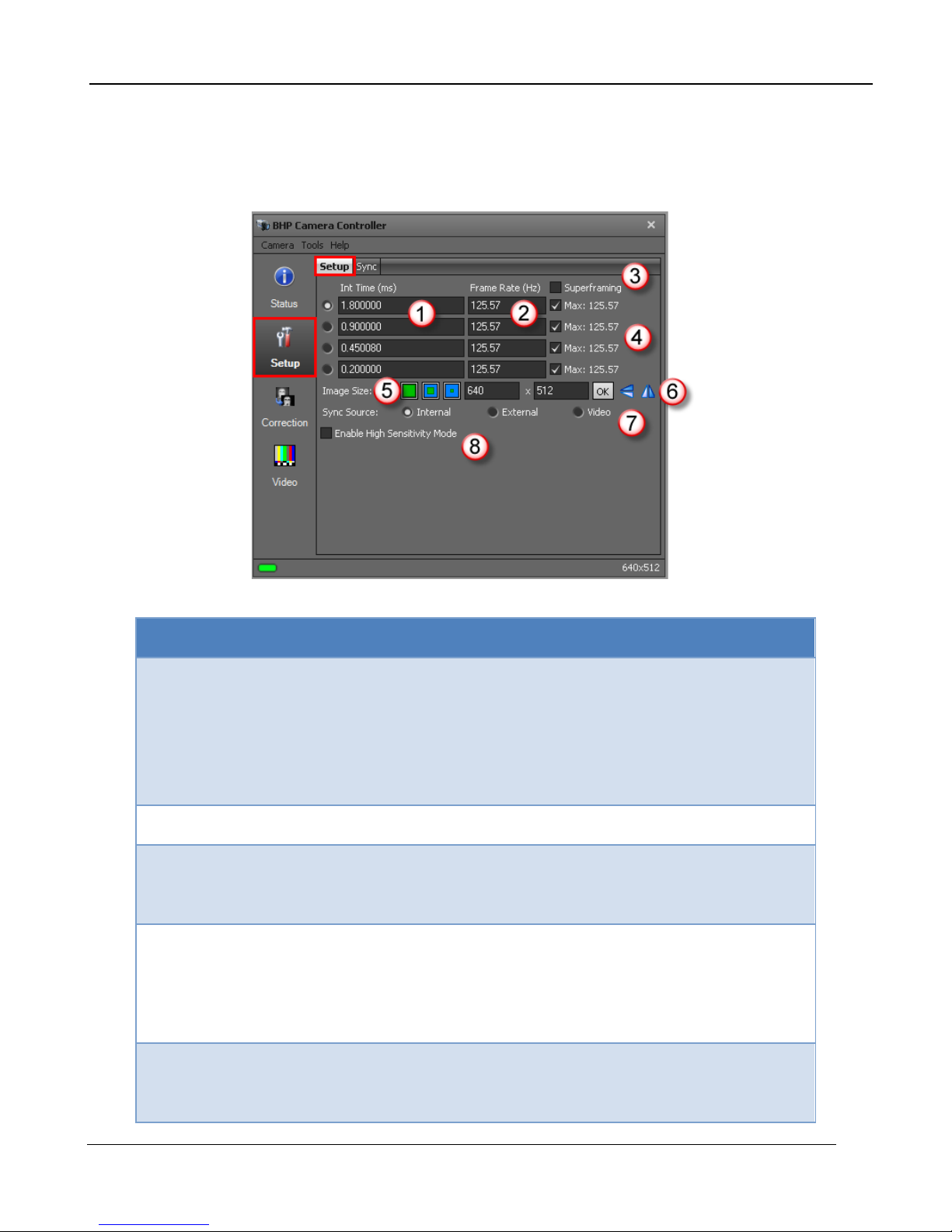
5.2.4 Setup Page

The Setup page allows the user to set integration time, frame rate, frame size, and Sync source.

5.2.4.1 Setup Tab

Item Name Description

Integration Time No factory calibration: Enter desired integration

time in milliseconds. With factory calibration: The box will have a

dropdown list with the available ranges. To manually enter integration time scroll to bottom of list and select “no factory calibration”.

2 3

Frame Rate Enter the desired frame rate in Hz.

Superframing

[A6750sc only]. When this is enabled the user can then select the presets to include and set the burst rate.

Max Frame Rate This indicates the max possible frame rate based

on the current window size and integration time. Checking the box will automatically keep the camera at max frame rate as these parameters change.

Image size A6700sc: This control will be simply a dropdown

A6700sc/A6750sc User’s Manual

list with the three window size options available (Full, ½, ¼).

Item Name Description

A6750sc: There are buttons to select Full, ½, ¼

windows as well as boxes to enter other sizes. Click “OK” to set a size. The box will turn red if the size is not valid.

5 –Camera Controller

Image Flipping

The icons control horizontal and vertical image flipping. With these controls, the flipping is done in the camera so both the digital and analog video are affected.

Sync Source Select internal, external, or video.

Internal: The frame sync is generated internally to run at the frequency set by the user

External: The frame sync is generated externally through the Sync In connect on the camer a rear chassis.

Video: The FPA frame sync is generated from the internal video encoder , locking the digital and analog clocks together

High Sensitivity Mode

(HSM)

HSM is a FLIR-patented algorithm first introduced in the Gas FindIR cameras that allows the user to see small temperature changes in the scene.

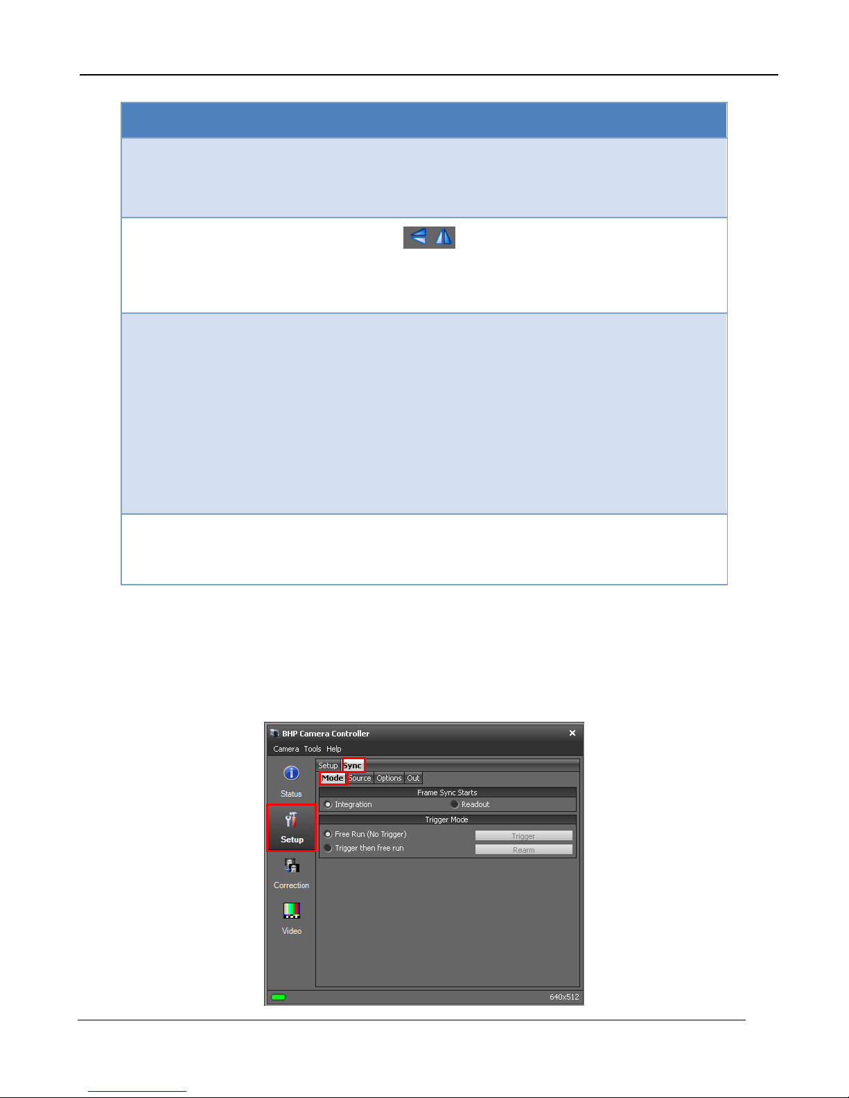
5.2.4.2 Sync Tab [A6750sc only]

The sync tab allows the user to control function for Syncs, and triggers. All of these sync features apply only to the A6750sc.

5.2.4.2.1 Sync Mode

A6700sc/A6750sc User’s Manual

5 –Camera Controller

Preset 0

Data

Frame Sync

Preset 1

Data

Preset 2

Data

Preset 3

Data

Frame Sync Frame Sync Frame Sync

Preset 3

Integration

Preset 2

Integration

Preset 1

Integration

Preset 0

Integration

5.2.4.2.1.1 Frame Sync Starts

The A6750sc makes use of frame syncs and triggers to control the generation of image data. Frame syncs control the start of individual frames whereas triggers start sequences of frames.

The generation of a frame consists of two phases: integration and data readout. Depending on the timing between these two events, you can have two basic integration modes: Integrate Then Read (ITR), and Integrate While Read (IWR). In ITR, integration and data readout occur sequentially. The complete frame time is the combined total of the integration time plus readout time. In IWR, the integration phase of the current frame occurs during the readout phase of the previous fra me. In other words, ITR and IWR terms refer to whether or not the camera will overlap the data readout and integration periods. In ITR, the data is not overlapped which means lower frame rates but provides a less noisy image. IWR can achieve much faster frame rates with a slight increase in noise. The A6750sc does not require the user to explicitly choose whether to operate in ITR or IWR modes. The camera will automatically select the integration mode based on the integration time, frame rate, and frame sync mode.

The A6750sc supports two Frame Sync Modes: Frame Sync Starts Integration (FSSI), and Frame Sync Starts Readout (FSSR). FSSI and FSSR determine which phase of the frame generation process (integration or data readout) is synchronized to the frame sync. FSSI starts the integration period when a frame sync occurs (i.e. “take a picture now”). The camera automatically calculates when to start data readout. FSSR starts the data readout (for the previous frame) when a frame sync occurs (i.e. “give me data now”). The camera automatically calculates when to start integration for the current frame. In FSSI mode, the camera could be in either ITR or IWR mode. In FSSR mode, the camera is always in IWR mode.

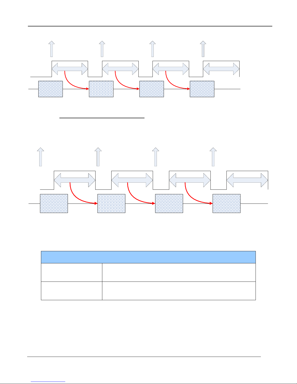
5.2.4.2.1.1.1 Frame Sync Starts Integration (FSSI) Upon frame sync, the camera immediately integrates followed by data read out. Based on integration

time, frame size, and frame rate, the camera will automatically choose ITR or IWR mode.

NOTE: When using an external frame sync and superframing, the external frame sy nc should be set

to comply with ITR frame rate limits. If the exte rnal syn c rate is to o fast, the camera w ill ignore syncs that come before the camera is ready

Figure 4-2: Frame Sync Starts Integration, ITR

A6700sc/A6750sc User’s Manual

5 –Camera Controller

Frame

1 Data

Frame 1 Integration

Frame 2 Integration

Frame Sync

Frame 2 Data

Frame 3 Integration

Frame Sync

Frame 3 Data

Frame 4 Integration

Frame Sync

Frame 1

Data

Frame 1 Integration

Frame 2 Integration

Frame Sync

Frame 2 Data

Frame 3 Integration

Frame Sync

Frame 3 Data

Frame 4 Integration

Frame Sync

Figure 4-3: Frame Sync Starts Integration, IWR

5.2.4.2.1.1.2 Frame Sync Starts Readout (FSSR) Upon frame sync, the camera immediately transmits the data from the previous frame. The

integration period is then placed to meet ROIC requirements. This mode always operates in IWR mode. This mode can be used with either internal or external frame sync at full frame rates.

Figure 4-4: Frame Sync Starts Readout

5.2.4.2.1.2 Trigger Mode

When the camera is placed in a triggered mode, the image stream will stop until the trigger is received.

Trigger Modes

Free Run (No Trigger)

Trigger then free run

In free run the camera cycles through frames/sequences continuously.

Upon receiving a trigger (external or software) the camera will start to generate sequences continuously.

A6700sc/A6750sc User’s Manual

5 –Camera Controller

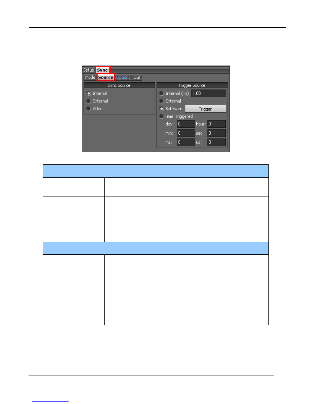
5.2.4.2.2 Sync Source

The Source options page allows the user to select the source for Syncs and Triggers.

Sync Sources

Internal

External

The frame sync is generated internally to run at the frequency set by the user

The frame sync is generated externally through the Sync In connect on the camera rear chassis.

The frame sync is generated from a external video source

Video

connected to the Gen Lock In connector on the camera rear chassis.

Trigger Sources

Internal

External

The tri gger is gener ated internally to run at the frequency set by the user (Hz).

The trigger is generated externally through the Trigger In connector on the camera rear chassis. (3.3V LVCMOS)

Software The trigger is generated via a software button (Trigger button)

Time Triggered

Camera generates an internal trigger when the internal timestamp clock reaches a specified time.

A6700sc/A6750sc User’s Manual

5 –Camera Controller

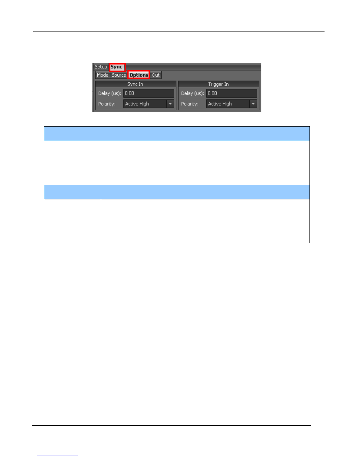
5.2.4.2.3 Sync Options

The Sync Options page allows the user to set delays and polarities for the Sync and Trigger In.

Sync In

Delay

Polarity

Delay

Polarity

Allows for the user to set a delay (µsec) for the external sync. See timing diagrams below.

The sync is edge triggered. Allows for the camera to use the rising or falling edge.

Allows for the user to set a delay (µsec) for the external trigger. See timing diagrams below.

Trigger is edge triggered. Allows for the camera to use the rising or falling edge.

Trigger In

A6700sc/A6750sc User’s Manual

5 –Camera Controller

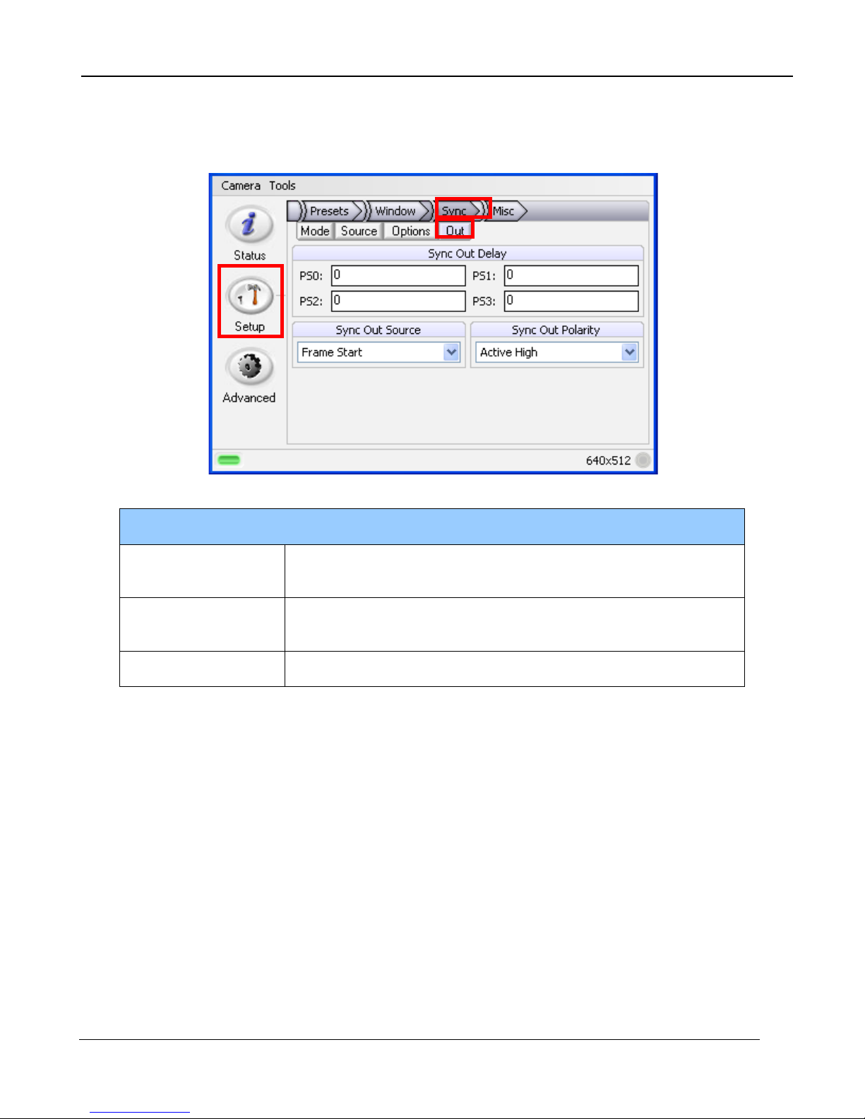
5.2.4.2.4 Sync Out

The Sync Out options allow the user to set a delay for the sync out pulse as well as the sync delay reference and polarity. The Sync Out signal always has a jitter of ±1 clock (160nsec).

Sync Out Options

Sync Out Delay Allows for the user to set a delay for the sync out on a preset

basis.

Sync Out Source Allows for the sync out to be referenced to the star t of frame or

start of integration.

Sync Out Polarity Allows for the sync out to be active high or low.

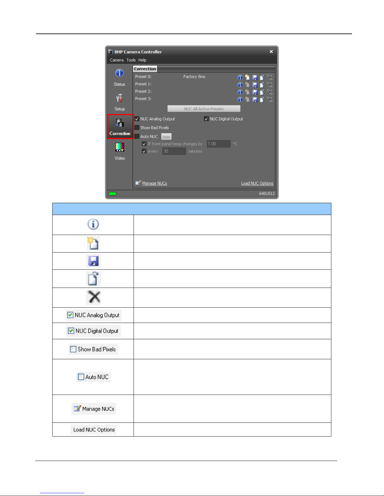
5.2.5 Correction Page

The Correction Tab contains all the controls needed to manage the on-camera NUCs. On-camera NUCs are stored in two types of memory:

RAM memory. This type of memory is used to store NUCs that will be applied to live image data. There is enough RAM memory for one NUC to be loaded for each Preset. This memory is volatile and is lost when then camera is turned off. If a NUC was loaded into RAM, the camera will reload that NUC from flash automatically when the camera is turned on if a Save State was performed.

Flash Memory. This type of memory is used as nonvolatile NUC storage. There is about 2GB of flash memory available for storing NUCs. This is enough space to store hundreds of full frame NUCs.

A6700sc/A6750sc User’s Manual

5 –Camera Controller

flag and perform a NUC Offset Update when selected criteria

Displays a list of NUCs stored in flash memory. User can

NUC Controls

NUC Info. Displays camera parameters and statistics related to the selected NUC

Perform NUC. Starts the NUC Wizar d.

Updates the current NUC to flash memory

Load a NUC from flash to RAM memory. Unload NUC from RAM mem ory. No on-camera NUC will be

applied to the data. Apply NUC to Analog video data

Apply NUC to Digital output (Gig E, CameraLink) Displays all pixels marked as “bad” as white dots on both the

analog and digital outputs. When enabled, the camera will automatically drop the internal

are met. The NUC update can be triggered on demand, by a change in the internal temperature sensor or by a ti mer

delete NUCs from flash memory as well as upload/download NUCs (.NPK files) from the host PC.

Displays options for loading NUCs.

A6700sc/A6750sc User’s Manual

5 –Camera Controller

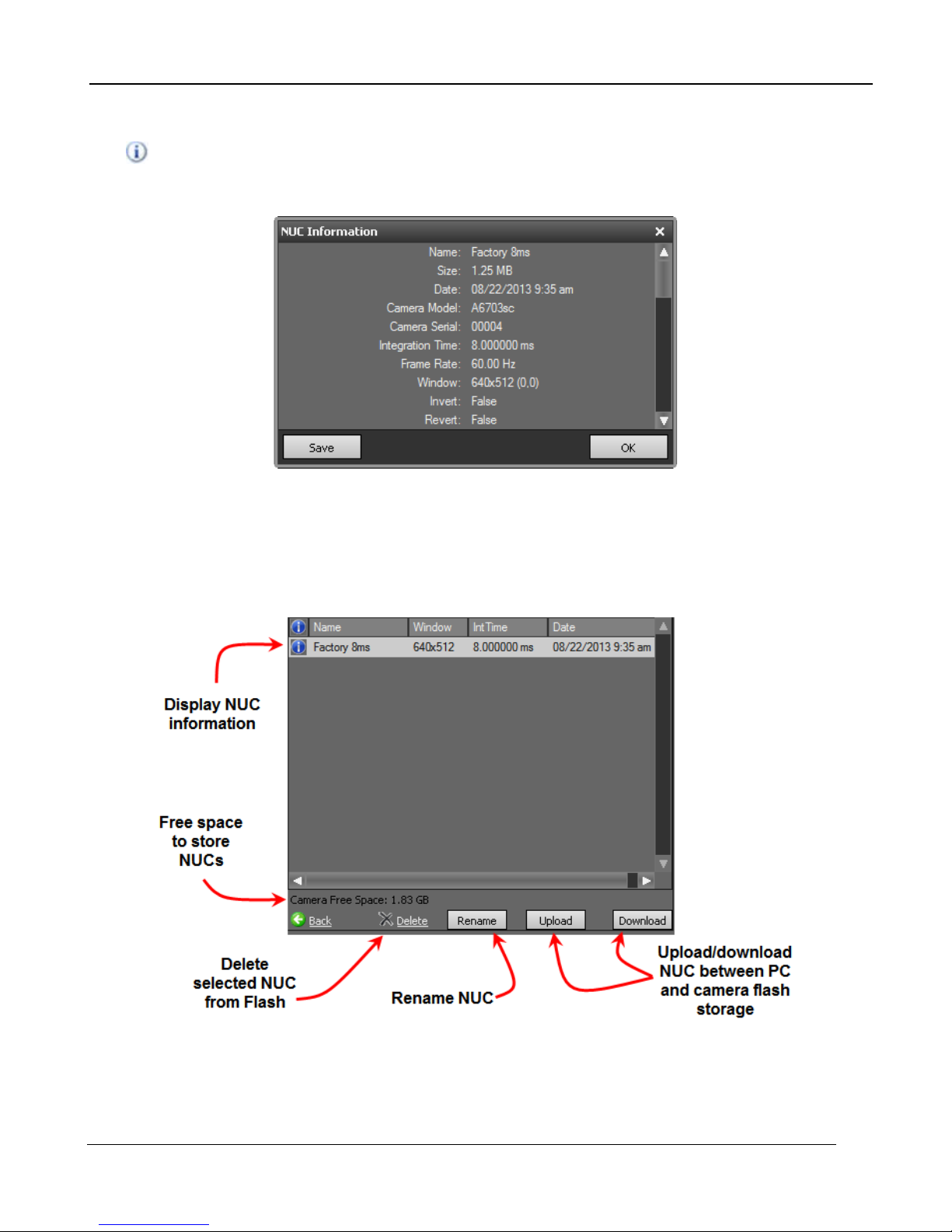
NUC Information

The button displays a list of camera parameters that are saved as part of the NUC as well as bad pixel statistics. Note that there is a scroll bar that can be used to see the whole list. The Save button allows the user to dump this list to a text file.

Manage NUCs

This dialog box allows the user to manage NUCs stored in non-volatile flash memory. Changes here will persists through a camera power cycle. For example, if you rename a NUC here and do not update the NUC loaded into RAM and the camera state, the camera will not be able to reload the NUC after a power cycle.

Load NUC Options

Typically, all of the camera configuration parameters are derived from the current Camera State. When the camera is powered up, it loads the last saved camera state. The names of the NUCs are stored as part of the state. Normally the NUC is performed with the settings that are eventually going

A6700sc/A6750sc User’s Manual

5 –Camera Controller

to be part of the state. If a NUC is loaded that has a setting that differs from the camera state, the state will override the NUC. If the user wants the NUC setting to override the state then “Load NUC Options” can be set.

The default setting is to “Load Table Only”, in which case only the NUC coefficients are used from a NUC file. When the user selects “Load Table and the Following Settings”, the user can select which parameters from the NUC will override the current state. The option will not affect NUCs that are currently loaded into RAM, only those NUCs that are subsequently loaded from Flash memory. Unless a new state is saved, these override settings will not be remembered after a power cycle.

Performing a NUC

To build a NUC table using the camera electronics, select the Perform Correction icon to start the NUC Wizard for the desired preset.

NOTE: Due to differences in camera electronics and FP A timi ngs i t is i mpo rtant to p erform the NUC

with the camera operatin g modes confi gured as it w ill be used w hen imaging.

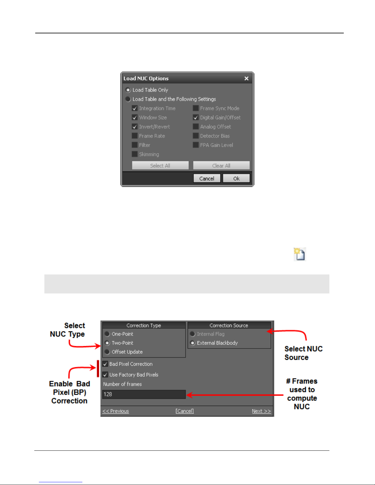
After selecting the Perform Correction a second window comes up to allow the user to select correction parameters. When all selections have been made, click Next>> to continue.

A6700sc/A6750sc User’s Manual

One Point

5 –Camera Controller

Correction (NUC) Types

Sets the gain terms to “1” and computes the offset terms. Uses a single NUC source. Does not compute a BP correction.

Two Point

Sets both the gain and offset terms. Uses two NUC sources. Computes a bad pixel correction.

Retains the current NUC gain terms and updates the offset

Offset Update

terms. Uses a single NUC source. Retains the current bad pixel (BP) correction.

Correction Sources

Use the internal flag as the NUC source. Because the flag

Internal Flag

is not temperature controlled, it can only be used for 1-point and Offset Update NUC functions

Use an external blackbody as the NUC source. Program

External Blackbody

will prompt the user to place each source in front of the camera. NUC source needs to fill the entire field of view.

Set the number of to average when computing NUC

Number of frames

coefficients. 16 frames is the default and works well for most scenarios. The value can be to be 2, 4, 8, 16, 32, 64, or 128.

After configuring the correction parameters and selecting Next>> the next window allows the user to set up the parameters used for the Bad Pixel Detection. Once the parameters are set, select Next>> to continue.

A6700sc/A6750sc User’s Manual

5 –Camera Controller

The next window allows the user to name the NUC. Simply type in the name for the table in the text box or select a previously saved file to replace it. Select Next>> to continue.

The next two screens will collect data from the NUC sources. If using the internal flag you will only see a few status messages. If using external blackbodies you will be prompted. After each step, click Next>> to continue.

The last screen gives a report of the bad pixels found. The dialog shows how many pixels failed in each category. If the result is satisfactory, click Accept to save the NUC. The NUC table will be stored to flash memory and loaded into RAM memory for that preset. If the NUC is poor and you want to abort, click[Discard].

NOTE: It is possible for a bad pixel to fail more than one category , so the total bad pixels may be less

than the sum of each category. “Fac tory” bad pixels are those that were deter mined to be bad during camera production testing.

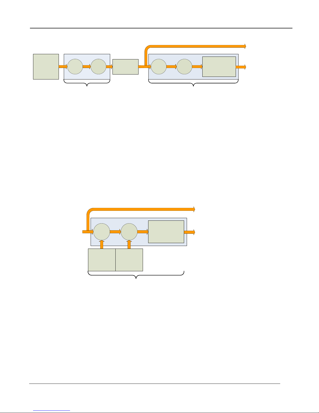
What is a Non-Uniformity Correction (NUC)?

Non-Uniformity Correction (NUC) refers the process by which the camera electronics correct for the differences in the pixel-to-pixel response for each individual pixel in the detector array. The camera can create (or allow for the user to load) a Non-Uniformity Correction (NUC) table which consists of a unique gain and offset coefficient and a bad pixel indicator for each pixel. The table is then applied in the digital processing pipeline as shown in Figure 4-12. The result is corrected data where each pixel responds consistently across the detector input range creating a uniform image.

A6700sc/A6750sc User’s Manual

5 –Camera Controller

Detector

-bit A/D

x +

NUC Table

Bad Pixel

Replacement

Algorithm

Corrected Data

Uncorrected Data

Analog

Gain/Offset

NUC Table

Bad Pixel

Replacement

Algorithm

Corrected Data

Uncorrected Data

“

1”

Offset

Coefficients

Figure 4-12: Digital Process Showing NUC Table Application

To create the NUC table, the camera images either one or two uniform temperature sources. The source can be an external source provided by the user or the camera’s internal NUC flag which is basically a shutter the camera places in front of the detector. If the source is external it should be uniform and large enough to overfill the cameras field-of-view (FOV). By analyzing the pixel data from these constant sources, the non-uniformity of the pixels can be determined and corrected. There are three types of processes which are used to create the NUC table; One-Point, Two-Point, and Offset Update.

5.2.5.1.1 One-Point Correction Process

A One-Point Correction Process requires one uniform source, which is typically in the middle of the usable range. The One-Point Correction replaces all gain coefficients in the NUC table with a value of one (“1”) as seen in Figure 4-13. The offset coefficients are computed uniquely for each pixel.

5.2.5.1.2 Two-Point Correction Process

The Two-Point Correction Process builds a NUC table that contains an individually computed gain and offset coefficient for each pixel as seen in Figure 4-14. Two uniform sources are required for this correction. One source at the low end and a second source at the upper end of the usable detector input range. Because of the use of two images at either end of the input range, the Two-Point Correction yields better correction results verses the One-Point process. A 2-point correct will also work better over a wider range of scene temperatures than a 1-point correction.

A6700sc/A6750sc User’s Manual

Figure 4-13: One-Point Correction

5 –Camera Controller

NUC Table

Bad Pixel

Replacement

Algorithm

Corrected Data

Uncorrected Data

Gain

Coefficients

Offset

Coefficients

NUC Table

Bad Pixel

Replacement

Algorithm

Corrected Data

Uncorrected Data

Bad Pixel

Indicator

Figure 4-14: Two-Point Correction

5.2.5.1.3 Offset Update

Often times during the normal operation of a camera the electronics and/or optics will heat up or cool down which changes the uniformity of the camera image. This change requires a new NUC. However, this change is mainly in the offset response of the image while the gain component stays constant. An Offset Update simply computes a new offset coefficient using the existing gain coefficient and corrects the image non-uniformity. Offsets Update are typically performed when a Two-Point NUC table is being used.

An Offset Update requires only one uniform source, usually set at a temperature on the lower edge of the operational range.

5.2.5.1.4 Bad Pixel Correction

Within the NUC table there is an indication as to whether or not a pixel has been determined to be bad as seen in Figure 4-15. There are two methods the A6700sc uses to determine bad pixels.

First, the NUC table gain coefficients are compared to a user defined acceptance boundary, Responsivity Limit Low/High (%). The responsivity of a pixel can be thought of as the gain of that pixel. The gain coefficient in the NUC Table is a computed value that attempts to correct the individual pixel gain, or responsivity, to a normalized value across the array. Since the responsivity

A6700sc/A6750sc User’s Manual

Figure 4-15: Bad Pixel Correction

5 –Camera Controller

value directly relates to the gain coefficient in the NUC table, the A6700sc can scan the NUC table gain coefficients and use them to determine if a pixel’s responsivity exceeds the limits as set by the user.

The second method of determining bad pixels is to search for twinklers. Twinklers are pixels that have responsivity values within normal tolerances, but still exhibit large swings for small input changes. These pixels are on the “verge” of being bad and often appear to be noisy. To find these types of pixels the camera collects N number of frames and records the maximum and minimum values across that sample set for each pixel. If the delta between max and min exceeds the Twinkler max pixel value delta then the pixel is determined to be bad.

Since the responsivity test requires a gain coefficient, it is useless on NUC tables determine by the One-Point Correction because those tables have a value of one (“1”) as the gain coefficients. The Twinkler test can be done on either correction process.

The A6700sc uses two algorithms for bad pixel replacement: 2-point Gradient, and Nearest Neighbor. The 2-point gradient algorithm is the default bad pixel correction method. With this algorithm, the two

pairs of pixels above and below and to the left and right of the bad pixel are evaluated. The algorithm compares the differences between the pixels and chooses the pair with smallest gradient (difference). It then averages the two adjacent pixels and uses that value for the replacement value. This algorithm is better at handling bad pixels near a high contrast edge and is the default method. If the algorithm encounters a situation is cannot solve (for example, an edge or corner) it will fall back on the nearest neighbor algorithm.

Nearest neighbor uses a simple replacement using an adjacent pixel. The adjacent pixel is picked using the pattern depicted below. When a bad pixel is near an edge, those search positions are skipped.

A6700sc/A6750sc User’s Manual

5 –Camera Controller

5.2.6 Video Page

The A6700sc camera has a 14-bit digital output. However, the analog output is only 8-bit. An Automatic Gain Control (AGC) algorithm is used to map the 14-bit digital to the 8-bit analog data. The Video Tab provides controls related to optimizing the Analog video output. These controls affect only the analog video. Figure 4-16 shows a flow chart of the analog video process and how the parameters of this screen are used.

Analog Video Setup Options

NTSC: 640x480, 30Hz interlaced, color based on Palette selection,

(Note: top and bottom 16 lines are truncated when full images are displayed. The Analog window can be adjusted +/- 16 rows using the

Format

Overlay Enables the analog video overlay.

Filter Rate Rate at which AGC is com puted (1 to 20 Hz)

Dampening

Setup>>Window Tab)

PAL: 640x480, 25Hz interlaced, color based on Palette selection

Note: When camera frame size is smaller than video frame size, black borders are added to maintain standard video output sizes

Rate at which AGC is allowed to change. This will keep the AGC from responding rapidly to fast tridents changes. Specified as a fraction from 0 to 1. This fraction is used as a weighting factor for the current AGC vs. the newly computed AGC.

A6700sc/A6750sc User’s Manual

AGC Mode

Corrected Data

Uncorrected Data

Mux

Plateau

Scalar

Linear Scalar

GUI: Plateau P

GUI: Bounds

Mux

GUI

: AGC Mode

Video

Encoder

GUI: Format

GUI: Position

GUI: Brightness

GUI: Contrast

Overlay

GUI: Overlay

GUI: NUC’d

Analog Video

Pallete

Scalar

GUI: Palette

5 –Camera Controller

Analog Video Setup Options

Plateau: Uses a plateau equalization (PE) algorithm to scale the image data for video display

DDE: Digital Detail Enhancement. Manual Linear: Scales the im age data to a windowed s ec tion of data range

as set by the user Auto Linear: Same as Manual Linear except camera analyzes image and

sets limits at ~1% and 98% of the histogram.

Plateau P

Bounds

DDE Sharpness

Scaling factor for the Plateau Equalization function Note: Plateau P is only visible when AGC Mode>> Plat eau is select ed Sets the lower and upper data range to be scaled to on the video data. Note: Bounds is only visible when AGC Mode>>Manual Linear is selected

Only visible when AGC is set to DDE. Selects the amount of enhancement processing.

Palette Allows user to select the color scheme to use on the analog video channel.

Allows user to set brightness and contrast on the video encoder. As shown

Brightness and

Contrast

in Figure 4-16, this occurs after the digital data has been scaled and converted to analog. These controls don’t tend to have as much effect as the controls that are applied to the digital side (before the video encoder).

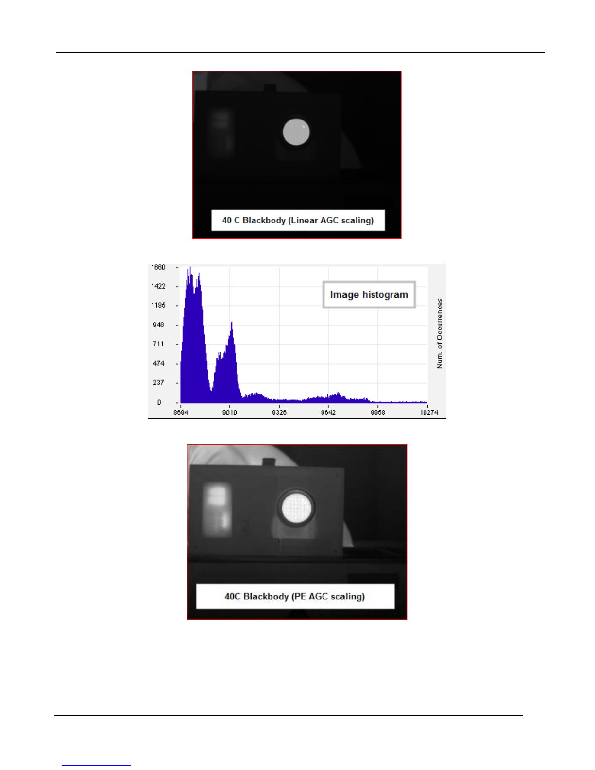
The Manual Linear algorithm evenly distributes the grayscale values over the digital values. This works fairly well if the image dynamic range is fairly evenly distributed but in general does not produce high contrast imagery, but it also does not saturate or clip the hot and cold regions either. The Plateau Equalization algorithm (also called PE) is a nonlinear AGC algorithm that uses the image histogram to optimally map the 256 gray scales. This algorithm works well for most scenes but it works best when the scene has a “bi-modal” distribution (two clumps). It usually the most popular because algorithm because it produces high contrast (but more saturated) video. The following pictures illustrate the differences in AGC algorithms. (The data was captured from the digital output but the effect is similar for the analog side.)

A6700sc/A6750sc User’s Manual

Figure 4-5: Analog Video Flow

5 –Camera Controller

One final note about the PE algorithm. It is very aggressive. It can pull detail out of very low contrast imagery. It can also pull out some very low-level NUC and FPA artifacts and noise if the contrast is low enough. This does not necessarily mean there is a problem with the camera, or NUC.

A6700sc/A6750sc User’s Manual

6 Interfaces

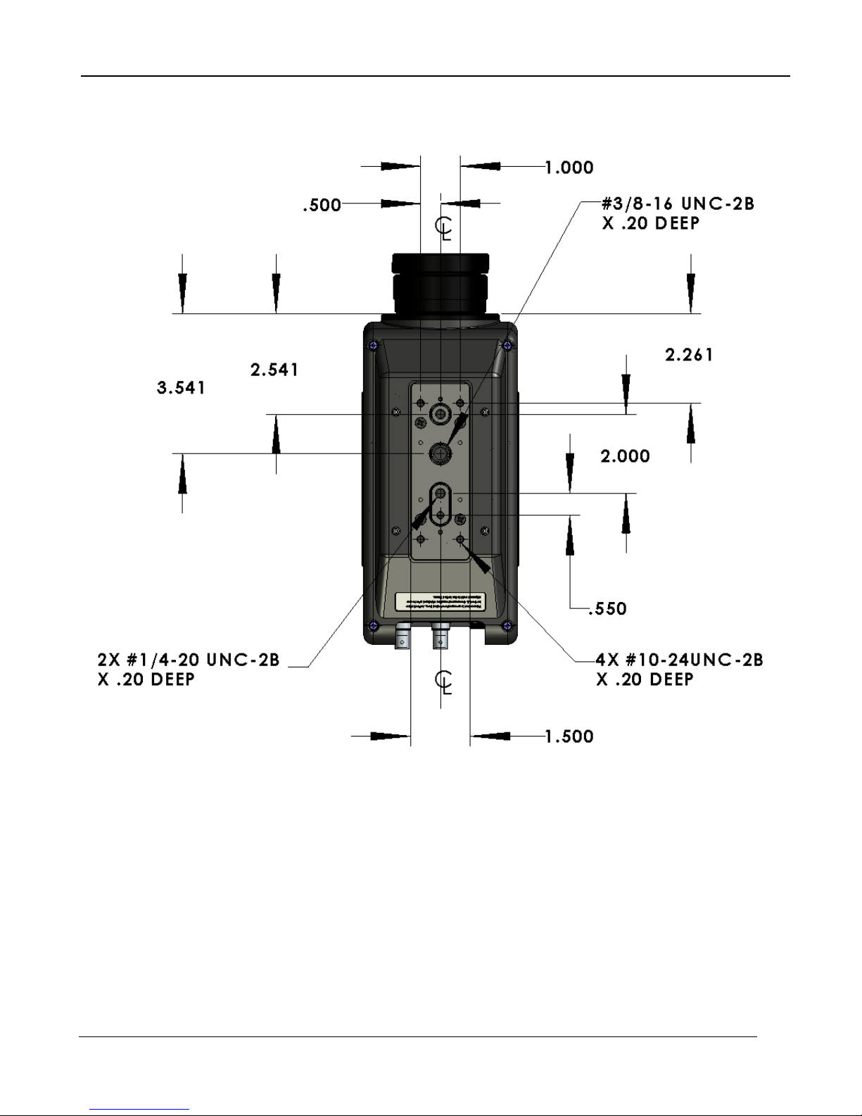
6.1 Mechanical (dimensions in inches)

6 – Interfaces

Figure 6-1: Front view of A6700sc

Figure 6-2: Side view of A6700sc with 50mm lens

A6700sc/A6750sc User’s Manual

6 – Interfaces

A6700sc/A6750sc User’s Manual

Figure 6-1: Bottom view of A6700sc

6 – Interfaces

6.1.1 Status Light s

The A6700sc provides a set of status indicators on the back panel to give the user some visual feedback on the camera operating state.

POWER (on power switch): Indicates that the camera is ON. READY: Camera electronics have completed boot up. Camera is

ready to accept commands. COLD: Indicates that the FPA has reached operating tem perature

(<80K).

6.1.2 Power Interface

24V DC nominal, external AC-DC power converter is provided with the A6700sc camera system as a standard accessory. Power supply specifications are:

Input voltage range: 100-250VAC 50/60Hz Current draw: 24 VDC at up to 4.0 amps input to the camera Converter dimensions: 6.25 inches x 3.5 inches x 2.75 inch (L x W x H) Converter weight: approximately 1 lb The power input pinouts are shown in Figure 6-4.

Figure 6-4: A6700sc Power Input Pinouts

When using your own DC power supply, you should take note of the following information: Output voltage: 24 VDC

Current draw: 1.4 amps nominal steady state, 2.6 amps peak (during cooldown) A6700sc power dissipation is <50 Watts steady state at nominal ambient temperature. Mating Connector: Fisher Connectors, S103A052-130+E31 103.1/5.7 +B. (FLIR PN 26399-000).

The power cable should be 20AWG (stranded 10/30), 3 conductor, no shield, max diameter of 0.223 inches. (Example: Alphawire PN 882003)

A6700sc/A6750sc User’s Manual

6 – Interfaces

6.1.3 Other Interfaces

6.1.3.1 Gigabit Ethernet

Gigabit Ethernet (GigE) is a common interface found in most PC’s. The GigE interface can be used for image acquisition and/or camera control. The GigE interface is GigE Vision compliant (for the image stream, but does not support Genicam for camera control).

6.1.3.2 Sync In

The Sync In can be selected, by the user, to operate as an external clock It is a rising edge LV-CMOS signal (5.5V max). The minimum width is 160nS.

6.1.3.3 Video

Composite video out (BNC connector). User selectable to be NTSC standard (640x480, 30Hz interlaced) or PAL standard (640x512, 25Hz interlaced). Video supports user selectable color palettes.

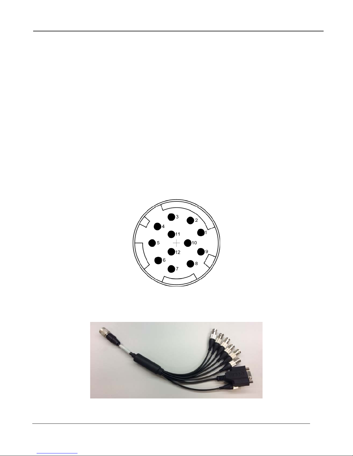
6.1.3.4 AUX Connector [A6750sc only]

The AUX connector provides access to additional signals. The diagram below shows a closeup view of the rear panel connector.

A breakout cable is provided with all A6750sc cameras.

A6700sc/A6750sc User’s Manual

6 – Interfaces

The provided breakout cable has numerical markings on the BNC overmolding that are described in the table below.

Pin Name Breakout

Type Description

Connector

RECORD START

SYNC OUT BNC 4 OUTPUT 160ns wide pulse at start of integration

GROUND

GPIO IN BNC 6 INPUT Sets bits in image header. Updated at ~1Hz rate.

Reserved BNC 7

TRIGGER BNC 8 INPUT External trigger. Can be used by ResearchIR to start

BNC 3 INPUT Sets bit in image header. Can be used by

ResearchIR to start recording.

recording.

Reserved BNC 9

SYNC IN BNC 10 INPUT Duplicate of rear panel input. Do not use both at the

same time.

RS-232 TX DB9 Male OUTPUT For camera control

RS-232 RX DB9 Male INPUT For camera control

Inputs are all LV-CMOS. High>2V, Low<0.2V. Max is 5.5V

If you wish to make your own breakout cable, there are three variants of the Hirose mating connector that will work: HR10A-10P-12S(73), HR10-10P-12S(73) or HR10A-10P-12SC(73).

A6700sc/A6750sc User’s Manual

7.1 Interface

7 – Specifications

7 Specifications

AC Power Control

Analog Video Out

Frame Sync In

Digital Video Out Optical Interface Thermal Interface

Mechanical Interface

7.2 Windowing Capacity

Window Sizes

90-230VAC, 50-60 Hz (using FLIR 24123-000 power supply) Genicam over Gigabit Ethernet (10/100/1000) Selectable

• NTSC/PAL selectable, BNC, 75Ω, 1V pk-pk

LVCMOS singled ended, BNC, selectable polarity, >160ns pulse width

14-bit Gigabit Ethernet (GigE Vision 2.0) Bayonet Semi-sealed enclosure with integral forced air heat exchanger 2 (two) ¼-20 tripod screws; 1 (one) 3/8-16 professional tripod

screw; 4 (four) 10-24 mount holes

640x512, 320x256, 160x120, [flexible for A6750sc]

Windowing Step Size Window Offset Step Size

16 columns, 4 rows (A6750sc) No offset, FPA centered

7.3 Acquisition Modes and Features

Frame Rate :

Max at Full Window

Max w/ Windowing

Max @ Min Window

Minimum

Resolution Pixel Rate (burst) Integration Width

Maximum

60 Hz for A6700, 125Hz for A6750sc 240 Hz @ ½ window, 480 Hz @ ¼ window (A6700sc) 406 Hz @ ½ window, 1063 Hz @ ¼ window (A6750sc) 4175 Hz @ 16x4 (A6750sc)

1.45mHz 160nS

50 MHz

98% selected frame time (1/frame rate)

A6700sc/A6750sc User’s Manual

7 – Specifications

Minimum

480 nS

Resolution Preset Sequencing

Digital Video Output

7.4 Analog Video

Video Output

Data Output

AGC

160 nS

• N/A

Selectable:

• Raw digital video (14-bits)

• Gain and offset (NUC) corrected (14-bits)

• NUC with bad pixel replaced (14-bits)

• NTSC or PAL composite

Selectable

• Raw, uncorrected

• Corrected

Selectable

• DDE

• Plateau based equalization

• Linear equalization

User controlled damping factor

AGC Filter

User controlled update rate

Overlay

Available on analog output Selectable

Palettes

• Grayscale

• Various color palettes

Auto-selected

Zoom (Analog video)

• x1 for 640x512

• x2 for 320x256 and 160x120 window sizes

Brightness and Contrast (analog video)

User controlled to increase or decrease

7.5 Performance Characteristics

Power Consumption

FLIR PWR Supply @ 120V

Continuous Cool Down: 50 VA

Continuous Normal: 41 VA

A6700sc/A6750sc User’s Manual

7 – Specifications

Power Consumption

Camera DC Power @ 24V

Cool-down Ti me Sensitivity (w/o optics)

NEΔT

1) NE∆T is at 50% nominal bucket fill, 298K background, + 5oC signal

Continuous Cool Down: 24 Watts

Continuous Normal: 21.25 Watts

≈7 minutes to reach operating temperature

18 mK typ .

7.6 Non Uniformity Correcti on

One Point (offset value with unity gain)

NUC Types

NUC Source

Bad Pixel Replacement

Two Point (offset and gain values) non-volatile Two Point w/Bad Pixel Detection/Replacement Update Offset (recalculates offset using current gain)

Internal: Ambient flag (for 1-pt and offset update only) External: Any user supplied source which covers entire FOV

Two-Point Gradient and neares t neighbor (autoselected)

Number of NUC’s

NUC Time NUC Performance

7.7 Detector/FPA

Spectral Response Detector Type f/# Integration Mode Format (HxV) Operability Charge Handling

Capacity Detector Pitch

4 active NUC’s in preset selectable form >100 NUCs in on-board flash

< 15 seconds

0.1%

3-5um (1-5um for broadband models) InSb f/2.5 or f/4 Snapshot 640 x 512 >99.8%, 99.95% typical

7.2 x106 e-

15 microns

Detector Cooling

A6700sc/A6750sc User’s Manual

Rotary Cryo Cooler

7.8 General Characteristics

7 – Specifications

Size

Length

Width

Height

Weight Temperature

Operating

Storage Shock Vibration Humidity Altitude Operating Orientation

8.5 inches

4.0 inches

4.3 inches (not including lens or lens cover)

5 lbs (not including lens or lens cover)

-40C to +50C

-55C to +80C 40 g’s, 11 msec half sine pulse

4.3 g's RMS random vibration, all three axes <95% relative humidity, non-condensing 0 to 10,000 feet operational, 0 to 70,000 feet non-operational No restriction in orientation

A6700sc/A6750sc User’s Manual

8 – Maintenance

8 Maintenance

8.1 Camera and Lens Cleaning

8.1.1 Camera Body, Cables and Accessories

The camera body, cables and accessories may be cleaned by wiping with a soft cloth. To remove stains, wipe with a soft cloth moistened with a mild detergent solution and wrung dry, then wipe with a dry soft cloth.

Do not use benzene, thinner, or any other chemical product on the camera, the cables or the accessories, as this may cause deterioration.

8.1.2 Lenses

It is recommends that all optics be handled with care and the need for cleaning is eliminated or at least reduced. If however,cleaning is deemed necessary, the methods herein are accepted industry standards and should yield good results.

Before you BEGIN,

Identify the type of optic to be cleaned.

▫ Is it hard or soft material? ▫ Is it coated & with what?

How is it contaminated?

▫ Particulate or film or both.

Set a standard of cleanliness.

▫ What is clean enough? ▫ Establish & document a standard.

Know your solvent.

▫ Read the MSDS ▫ See recommended solvents

Assemble your supplies:

▫ Latex gloves ▫ Clean, well-lit work area ▫ Inspection light ▫ Lens tissue or cloth ▫ Dust bulb or filtered air ▫ Proper solvent ▫ Solvent dispenser

The Drag Wipe Method: Set-up a clean area to work from with an anti-roll barrier around the edge to prevent anything from

leaving the table. Use a clean, lint free cloth or lens tissue. Wear latex gloves - clean them with alcohol or detergent before handling optic.

A6700sc/A6750sc User’s Manual

8 – Maintenance

NEVER touch the face of the optic. Cover the optic and store in a dry - dust free area immediately after cleaning.

1. Blow or brush loose particles from surface. Don’t let them contaminate your work area. Use air from a can or a filtered source.

2. Apply solvent directly to your cloth. Use slow, even, light pressure working from edge to edge across the optic.

Recommended Solvents

Material Solvent

Fused Silica 1,2,3,4 Zinc Selenide 1,2,4

BK-7 1,2,3,4 Zinc Sulfide 1,2,4

Optical Crown Glass 1,2,3,4 Sapphire 1,2,3,4

Zerodur 1,2,3,4

Calcium Fluoride 1,2,4 Coated Optics

Magnesium Fluoride 1,2,4 Dielectric coating 1,2,3,4

Sodium Chloride Nitrogen Interference filters 3

Potassium Chloride Nitrogen Soft metallic coating Air only

Potassium Bromide Nitrogen Hard/Protected metallic 1,2,3,4

Thallium Bromoiodide Nitrogen

1] Water free Acetone 2] Ethanol 3] Methanol 4] Isopropanol

A6700sc/A6750sc User’s Manual

9 – Infrared Primer

9 Infrared Primer

9.1 History of Infrared

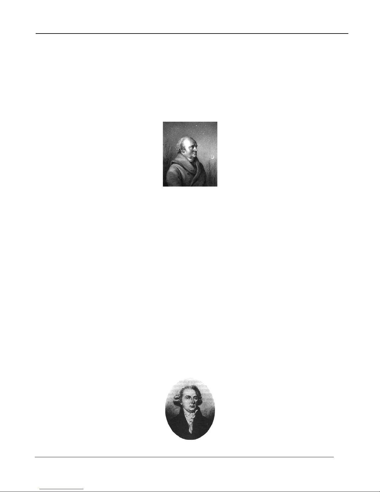
Less than 200 years ago the existence of the infrared portion of the electromagnetic spectrum wasn't even suspected. The original significance of the infrared spectrum, or simply ‘the infrared’ as it is often called, as a form of heat radiation is perhaps less obvious today than it was at the time of its discovery by Herschel in 1800.

Figure 8-1: Sir William Herschel (1738–1822)

The discovery was made accidentally during the search for a new optical material. Sir William Herschel – Royal Astronom er to King George III of England, and already famous for his discovery of the planet Uranus – was searching for an optical filter material to reduce the brightness of the sun’s image in telescopes during solar observations. While testing different samples of colored glass which gave similar reductions in brightness he was intrigued to find that some of the samples passed very little of t he sun’s heat, while others passed so much heat that he risked eye damage aft er only a few seconds’ observation.

Herschel was soon convinced of the necessity of setting up a systematic experiment, with the objective of finding a single material that would give the desired reduction in brig htness as well as the maximum reduction in heat. He began the experiment by actually repeating Newton’s prism experiment, but looking for the heating effect rather than the visual distribution of intensity in the spectrum. He first blackened the bulb of a sensitive mercury-in-glass thermometer with ink, and with this as his radiation detector he proceeded to test the heating effect of the various colors of the spectrum formed on the top of a table by passing sunlight t hrough a g lass prism. Other thermometers, placed outside the sun’s rays, served as controls.

As the blackened thermometer was moved slowly along the colors of the spectrum, the temperature readings showed a steady increase from the violet end to the red end. This was not entirely unexpected, since the Italian researcher, Landriani, in a similar experiment in 1777 had observed much the same effect. It was Herschel, however, who was the f irst to recognize that there must be a point where the heating effect reaches a maximum, and those measurements confined to the visible portion of the spectrum failed to locate this point.

A6700sc/A6750sc User’s Manual

9 – Infrared Primer

Figure 8-2: Marsilio Landriani (1746–1815)

Moving the thermometer into the dark region beyond the red end of the spectrum, Her s c h el c onfirmed that the heating continued to increase. The maximum point, when he found it, lay well beyond the red end – in what is known today as the ‘infrared wavelengths’.

When Herschel revealed his discovery, he referred to this new portion of the electromagnetic spectrum as the ‘thermometrical spectrum’. The radiation itself he sometimes referred to as ‘dark heat’, or simply ‘the invisible rays’. Ironically, and contrary to popular opinion, it wasn't Herschel who originated the term ‘infrared’. The word only began to appear in print around 75 years later, and it is still unclear who should receive credit as the originator.

Herschel’s use of glass in the prism of his original experiment led to some early controversies with his contemporaries about the actual existence of the infrared wavelengths. Different investigators, in attempting to confirm his work, used various types of glass indiscriminately, having different transparencies in the infrared. Through his later experiments, Herschel was aware of the limited transparency of glass to the newly-discovered thermal radiation, and he was forced to conclude that optics for the infrared would probably be doomed to the use of reflective elements exclusively (i.e. plane and curved mirrors). Fortunately, this proved to be true only until 1830, when the Italian investigator, Melloni, made his great disc overy that naturally occurring rock salt (NaCl) – whic h was available in large enough natural crystals to be made into lenses and prisms – is remarkably transparent to the infrared. The result was that rock salt became the principal infrared optical material, and remained so for the next hundred years, until the art of synthetic crystal growing was mastered in the 1930’s.

Figure 8-3: Macedonio Melloni (1798–1854)

Thermometers, as radiation detectors, remained unchallenged until 1829, the year Nobili invented the thermocouple. (Herschel’s own thermometer could be read to 0.2 °C (0.036 °F), and later models were able to be read to 0.05 °C (0.09 °F)). Then a breakthrough occurred; Melloni connected a number of thermocouples in series to form the first thermopile. The new device was at least 40 times as sensitive as the best thermometer of the day for detecting heat radiation – capable of detecting the heat from a person standing three meters away.

The first so-called ‘heat-picture’ became possible in 1840, the result of work by Sir John Herschel, son of the discoverer of the infrared and a famous astronomer in his own right. Based upon the differential evaporation of a thin film of oil when exposed to a heat pattern focused upon it, the thermal image could be seen by reflected light where the interference effects of the oil film made the image visible to the eye. Sir John also m anaged to obtain a primitive record of the thermal image on paper, which he called a ‘thermograph’.

A6700sc/A6750sc User’s Manual

9 – Infrared Primer

Figure 8-4: Samuel P. Langley (1834–1906)

The improvement of infrared-detector sensitivity progressed slowly. Another major breakthrough, made by Langley in 1880, was the invention of the bolometer. This consisted of a thin blackened strip of platinum connected in one arm of a Wheatstone bridge circuit upon which the infrared radiation was focused and to which a sensitive galvanometer responded. This instrument is said to have been able to detect the heat from a cow at a distance of 400 meters.

An English scientist, Sir James Dewar, first introduced the use of liquefied gases as cooling agents (such as liquid nitrogen with a temperature of -196 °C (-320. 8 °F)) in low temperature research. In 1892 he invented a unique vacuum insulating container in which it is possible to store liquefied gases for entire days. The common ‘thermos bottle’, used for storing hot and c old drinks, is based upon his invention.

Between the years 1900 and 1920, the inventors of the world ‘discovered’ the infrared. Many patents were issued for devices to detect personnel, artillery, aircraft, ships – and even icebergs. The first operating systems, in the modern sense, began to be developed during the 1914–18 war, when both sides had research programs devoted to the military exploitation of the infrared. These programs included experimental systems for enemy intrusion/detection, remote temperature sensing, secure communications, and ‘flying torpedo’ guidance. An infrared search system tested during this period was able to detect an approaching airplane at a distance of 1.5 km (0.94 miles), or a person more than 300 meters (984 ft.) away.

The most sensitive systems up to this time were all based upon variations of the bolometer idea, but the period between the two wars saw the development of two revolutionary new infrared detectors: the image converter and the photon detector. At first, the image converter received the greatest attention by the military, because it enabled an observer for the first time in history to literally ‘see in the dark’. However, the sensitivity of the image converter was limited to the near infrared wavelengths, and the most inter esting military targets (i.e. enemy soldiers) had to be illuminated by infrared search beams. Since this involved the risk of giving away the observer’s position to a similarly-equipped enemy observer, it is underst andable that military interest in the imag e converter eventually faded.

The tactical military disadvantages of so-called 'active’ (i.e. search beam-equipped) thermal imaging systems provided impetus following the 1939–45 war for extensive secret military infrared-research programs into the possibilities of developing ‘passive’ (no search beam) systems around the extremely sensitive photon detector. During this period, military secrecy regulations completely prevented disclosure of the status of infrare d -imaging technology. This secrecy only began to be lifted in the middle of the 1950’s, and from that time adequate thermal-imaging devices finally began to be available to civilian science and industry.

A6700sc/A6750sc User’s Manual

9 – Infrared Primer

9.2 Theory of Thermography

9.2.1 Introduction

The subjects of infrared radiation and the related technique of thermography are still new to many who will use an infrared camera. In this section the theory behind thermography will be given.

9.2.2 The Electromagnetic Spectrum

The electromagnetic spectrum is divided arbitrarily into a number of wavelength regions, called bands, distinguished by the methods used to produce and detect the radiation. There is no fundamental difference between radiation in the different bands of the electromagnetic spectrum. They are all governed by the same laws and the only differences are those due to differences in wavelength.

Figure 8-5 The Electromagnetic Spectrum

1: X-ray; 2: UV; 3: Visible; 4: IR; 5: Microwaves; 6: Radiowaves.

Thermography makes use of the infrared spectral band. At the short -wavelength end the boundary lies at the limit of visual perception, in the deep red. At the longwavelength end it merges with the microwave radio wavelengths, in the millimeter range.

The infrared band is often further subdivided into four smaller bands, the boundaries of which are also arbitrarily chosen. They include: the near infrared (0.75–3 μm), the middle infrared (3–6 μm), t he far infrared (6–15 μm) and the extreme infrared (15–100 μm). Although the wavelengths are given in μm (micrometers), other units are often still used to measure wavelength in this spectral region, e.g. nanometer (nm) and Ångström (Å). The relationships between the different wavelength measurements is:

9.2.3 Blackbod y Radiation

A blackbody is defined as an object which absorbs all radiation that impinges on it at any wavelength. The apparent misnomer black relating to an object emitting radiation is explained by Kirchhoff’s Law

A6700sc/A6750sc User’s Manual

9 – Infrared Primer

(after Gustav Robert Kirchhoff, 1824–1887), which states that a body capable of absorbing all radiation at any wavelength is equally capable in the emission of radiation.

Figure 8-6: Gustav Robert Kirchhoff (1824–1887)

The construction of a blackbody source is, in principle, very simple. The radiation characteristics of an aperture in an isotherm cavity made of an opaque absorbing material represents almost exactly the properties of a blackbody. A practical application of the principle to the construction of a perfect absorber of radiation consists of a box that is light tight except for an aperture in one of the sides. Any radiation which then enters the hole is scattered and absorbed by repeated reflections so only an infinitesimal fraction can possibly escape. The blackness which is obtained at the aperture is nearly equal to a blackbody and almost perfect for all wavelengths.

By providing such an isothermal cavity with a suitable heater it becomes what is termed a cavity radiator. An isothermal cavity heated to a uniform temperature generates blackbody radiation, the characteristics of which are determined solely by the temperature of the cavity. Such cavity radiators are commonly used as sources of radiation in temperature reference standards in the laboratory for calibrating thermographic instruments, such as a FLIR Systems camera for example.

If the temperature of blackbody radiation increases to more than 525 °C (977 °F), the source begins to be visible so that it appears to the eye no longer black. This is the incipient red heat temperature of the radiator, which then becomes orange or yellow as the temperature increases further. In fact, the definition of the so-called color temperature of an object is the temperature to which a blackbody would have to be heated to have the same appearance. Now consider three expressions that describe the radiation emitted from a blackbody.

Planck’s Law

Figure 8-7: Max Planck (1858–1947)

Max Planck (1858–1947) was able to describe the spectral distribution of the radiation from a blackbody by means of the following formula:

A6700sc/A6750sc User’s Manual

9 – Infrared Primer

Where:

Wλb = Blackbody spectral radiant emittance at wavelength λ. c = Velocity of light = 3 × 108 m/s h = Planck’s constant = 6.6 × 10-34 Joule sec. k = Boltzmann’s constant = 1.4 × 10-23 Joule/K. T = Absolute temperature (K) of a blackbody.

λ = Wavelength (μm).

Note

The factor 10-6 is used since spectral emittance in the curves is expressed in Watt/m2 m. If the factor is excluded, the dim ension w ill be Watt/m2μm.

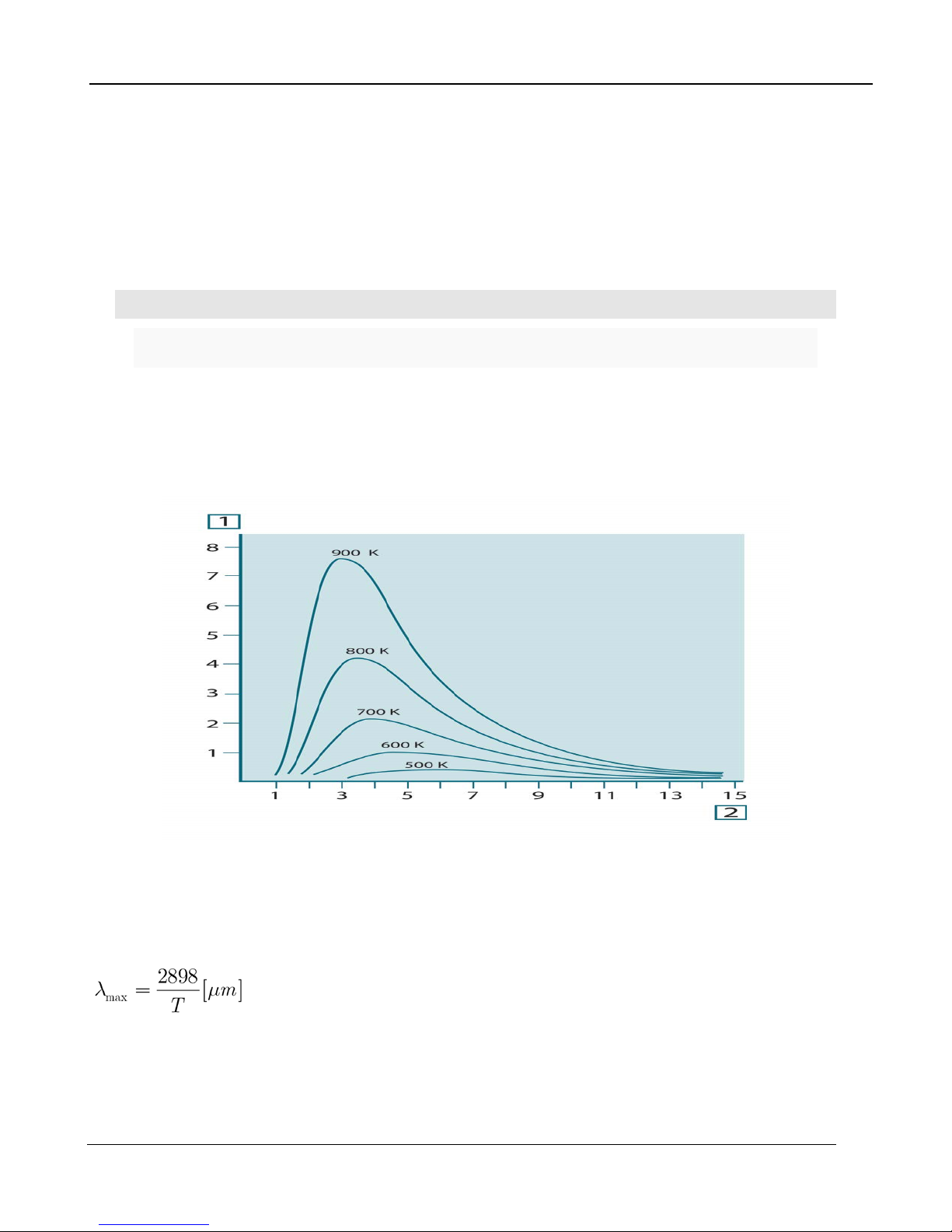
Planck’s formula, when plotted graphically for various temperatures, produces a family of curves. Following any particular Planck curve, the spectral emittance is zero at λ = 0, then increases r apidly to a maximum at a wavelength λmax and after passing it approaches zero again at very long wavelengths. The higher the temperature, the shorter the wavelength at which maximum occurs.

Figure 8-8: Blackbody spectral radiant emittance according to Planck’s law, plotted for various

absolute temperatures. 1: Spectral radiant emittance (W/cm2 × 103(μm)); 2: Wavelength (μm)

Wien’s Displacement Law

By differentiating Planck’s formula with respect to λ, and finding the maximum, we have:

This is Wien’s formula (after Wilhelm Wien, 1864–1928), which expresses mathematically the common observation that colors vary from red to orange or yellow as the temperature of a thermal radiator increases. The wavelength of the color is the same as the wavelength calculated for λmax. A good approximation of the value of λma x for a g iven blackbody temperature is obtained by applying

A6700sc/A6750sc User’s Manual

9 – Infrared Primer

the rule-of-thumb 3 000/T μm. Thus, a very hot star such as Sirius (11 000 K), em itting bluish-white light, radiates with the peak of spectral radiant emittance occurring within the invisible ultraviolet spectrum, at wavelength 0.27 μm.

Figure 8-9: Wilhelm Wien (1864–1928)

The sun (approx. 6 000 K) emits yellow light, peaking at about 0.5 μm in the middle of the visible light spectrum.

At room temperature (300 K) the peak of radiant emittance lies at 9.7 μm, in the f ar infrared, while at the temperature of liquid nitrogen (77 K) the maximum of the almost insignificant amount of radiant emittance occurs at 38 μm, in the extreme infrared wavelengths.

Figure 8-10: Planckian curves plotted on semi-log scales from 100 K to 1000 K. The dotted line

represents the locus of maximum radiant emittance at each temperature as described by

Wien's displacement law. 1: Spectral radiant emittance (W/cm2 (μm)); 2: Wavelength (μm).

Stefan-Boltzmann's Law

By integrating Planck’s form ula from λ = 0 to λ = ∞, we obtain the total r adiant emittance (Wb) of a blackbody:

A6700sc/A6750sc User’s Manual

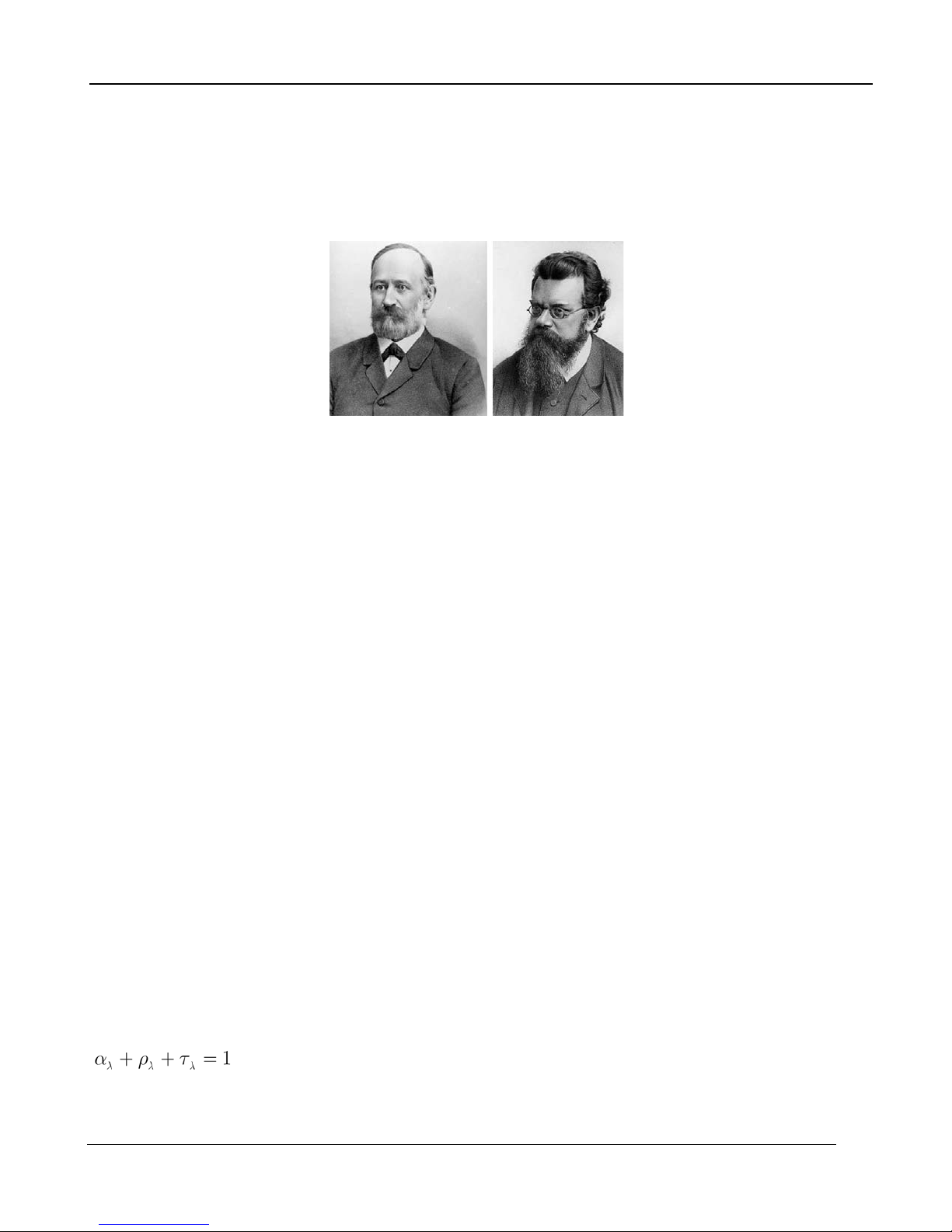
9 – Infrared Primer

This is the Stefan-Boltzmann formula (after Josef Stefan, 1835–1893, and Ludwig Boltzmann, 1844–

1906), which states that the total emissive power of a blackbody is proportional to the fourth power of its absolute temperature. Graphically, Wb represents the area below the Planck curve for a particular temperature. It can be shown that the radiant emittance in the interval λ = 0 t o λmax is only 25 % of the total, which represents about the amount of the sun’s radiation which lies inside the visible light spectrum.

Figure 8-11: Josef Stefan (1835–1893), and Ludwig Boltzmann (1844–1906)

Using the Stefan-Boltzmann formula to calculate the power radiated by the human body, at a temperature of 300 K and an external surface area of approx. 2 m2, we obtain 1 kW. This power loss could not be sustained if it were not for the compensating absorption of radiation from surrounding surfaces, at room temperatures which do not vary too drastically from the temperature of the body – or, of course, the addition of clothing.

Non-Blackbody Emitters

So far, only blackbody radiators and blackbody radiation have been discussed. However, real objects almost never comply with these laws over an extended wavelength region – although they may approach the blackbody behavior in certain spectral intervals. For example, a certain type of white

paint may appear perfectly white in the visible light spectrum, but becomes distinctly gray at about 2 μ m, and beyond 3 μm it is almost black.

There are three processes which can occur that prevent a real object from acting like a blackbody: a fraction of the incident radiation α may be absorbed, a fraction ρ may be reflected, and a fraction τ

may be transmitted. Since all of these factors are more or less wavelength dependent, the subscript λ is used to imply the spectral dependence of their definitions. Thus:

The spectral absorptance αλ= the ratio of the spectral radiant power absorbed by an object to that incident upon it.

The spectral reflectance ρλ = the ratio of the spectral radiant power reflected by an object to that incident upon it.

The spectral transmittance τλ = the ratio of the spectral radiant power transmitted thr o ug h an o b j ec t to that incident upon it.

The sum of these three factors must always add up to the whole at any wavelength, so we have the relation:

For opaque materials τ

λ = 0 and the relation simplifies to:

A6700sc/A6750sc User’s Manual

9 – Infrared Primer

Another factor, called the emissivity, is required to describe the fraction ε of the radiant emittance of a blackbody produced by an object at a specific temperature. Thus, we have the definition: The spectral emissivity ε

λ= the ratio of the spectral radiant power from an object to that from a blackbody at the

same temperature and wavelength. Expressed mathematically, this can be written as the ratio of the spectral emittance of the object to that of a blackbody as follows:

Generally speaking, there are three types of radiat ion source, distinguished by the ways in which the spectral emittance of each varies with wavelength.

A blackbody, for which ελ = ε = 1 A graybody, for which ελ = ε = constant less than 1 A selective radiator, for which ε varies with wavelength According to Kirchhoff’s law, for any material the spectral emissivity and spectral absorptance of a

body are equal at any specified temperature and wavelength. That is:

From this we obtain, for an opaque material (since α

λ + ρλ = 1):

For highly polished materials ε

λ approaches zero, so that for a perfectly reflecting material (i.e. a

perfect mirror) we have:

For a graybody radiator, the Stefan-Boltzmann formula becomes:

This states that the total emissive power of a graybody is the same as a blackbody at the same temperature reduced in proportion to the value of ε from the graybody.

A6700sc/A6750sc User’s Manual

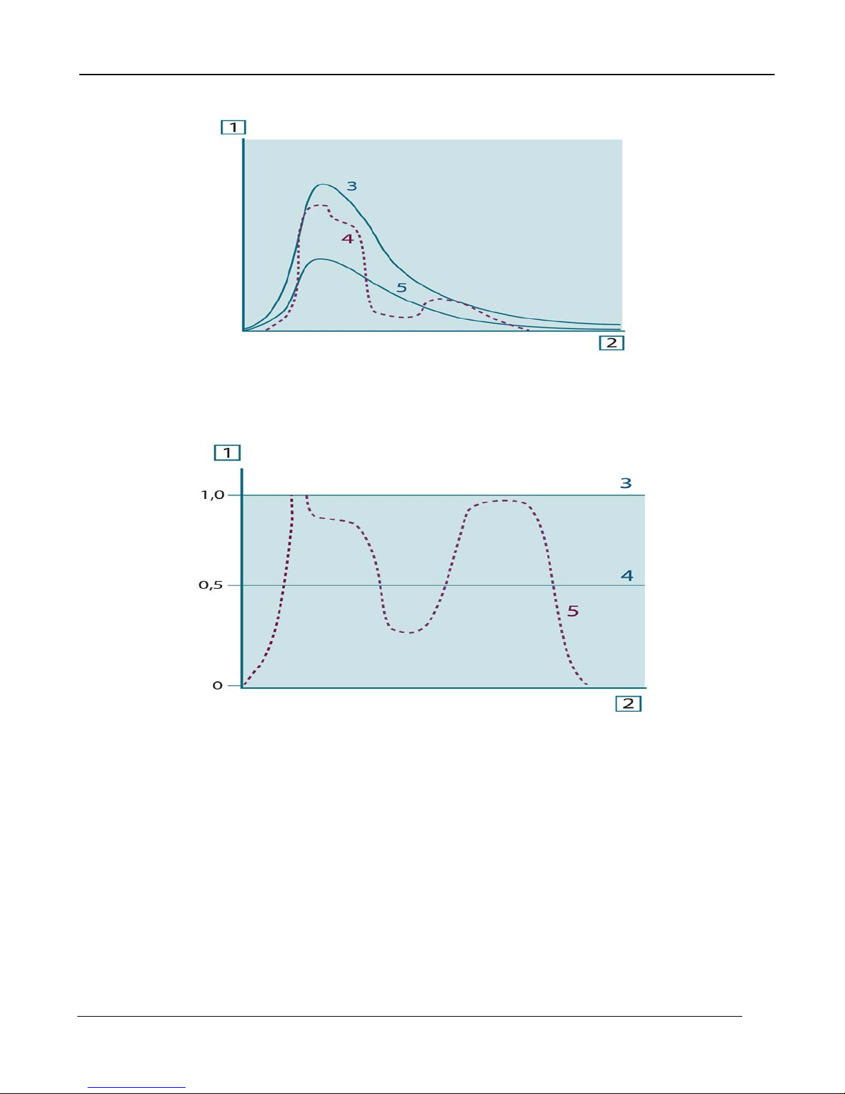
9 – Infrared Primer

Figure 8-12: Spectral radiant emittance of three types of radiators. 1: Spectral radiant

emittance; 2: avelength; 3: Blackbody; 4: Selective radiator; 5: Graybody.

Figure 8-13: Spectral emissivity of three types of radiators. 1: Spectral emissivity; 2:

Wavelength; 3: blackbody; 4: Graybody; 5: Selective radiator.

9.2.4 Infrared Semi-Transparent Materials

Consider now a non-metallic, semi-transparent body – let us say, in the form of a thick flat plate of plastic material. When the plate is heated, radiation generated within its volume must work its way toward the surfaces through the material in which it is partially absorbed. Moreover, when it arrives at the surface, some of it is reflected back into the interior. The back-reflected radiation is again partially absorbed, but some of it arrives at the other surface, through which most of it escapes; part of it is reflected back again. Although the progressive reflections become weaker and weaker they must all be added up when the total emittance of the plate is sought. W hen the resulting geometrical series is summed, the ef fecti ve emissivity of a semi-transparent plate is obtained as:

A6700sc/A6750sc User’s Manual

9 – Infrared Primer

When the plate becomes opaque this formula is reduced to the single formula:

This last relation is a particularly convenient one, because it is often easier to measure reflectance than to measure emissivity directly.

9.3 The Measurement Formula

As already mentioned, when viewing an object, the camera receives radiation not only from the object itself. It also collects radiation from the surroundings reflected via the object surface. Both these radiation contributions become attenuated to some extent by the atmosphere in the measurement path. To this comes a third radiation contribution from the atmosphere itself.

This description of the measurement situation, as illustrated in the figure below, is so far a fairly true description of the real conditions. What has been neglected could for instance be sun lig ht scattering in the atmosphere or stray radiation from intense radiation sources outside the field of view. Such disturbances are difficult to quantify, however, in most cases they are fortunately small enough to be neglected. In case they are not negligible, the measurement configuration is likely to be such that the risk for disturbance is obvious, at least to a tr ained operator. It is then his r esponsibility to modify the measurement situation to avoid the disturbance e.g. by changing the viewing direction, shielding off intense radiation sources etc.

Accepting the description above, we can use the figure below to derive a formula for the calculation of the object temperature from the calibrated camera output.

Figure 8-14: A schematic representation of the general thermographic measurement

situation.1: Surroundings; 2: Object; 3: Atmosphere; 4: Camera

A6700sc/A6750sc User’s Manual

9 – Infrared Primer

Assume that the received radiation power W from a blackbody source of temperature Tsource on short distance generates a camera output signal U

source that is proportional to the power input (power linear

camera). We can then write (Equation 1):

Where C i s a const ant. Should the source be a graybody with emittance ε, the received radiation would consequently be ε

source.

We are now ready to write the three collected radiation power terms:

1. Emission from the object = ετWobj, where ε is the emittance of the object and τ is the transmittance of the atmosphere. The object temperature is Tobj.

2. Reflected emission from am bient sources = (1 – ε)τWrefl, where (1 – ε) is the reflectance of the object. The ambient sources have the temperature Trefl.

It has here been assumed that the temperature T

refl is the same for all emitting surfaces within the

halfsphere seen from a point on the object surface. This is of course sometimes a simplif ication of the true situation. It is, however, a necessary simplification in order to derive a workable formula, and T

refl

can – at least theoretically – be given a value that represents an efficient temperature of a complex surrounding.

Note also that we have assumed that the emittance for the surroundings = 1. This is correct in accordance with Kirchhoff’s law: All radiation impinging on the surrounding surfaces will eventually be absorbed by the same surfaces. Thus the emittance = 1.

Note

Though that the latest discussion requires the complete sphere around theobject to be considered.

3. Emission from the atmosphere = (1 – τ)τWatm, where (1 – τ) is the emittance of the atmosphere. The temperature of the atmosphere is Tatm.

The total received radiation power can now be written (Equation 2):

We multiply each term by the constant C of Equation 1 and replace the CW products by the corresponding U according to the same equation, and get (Equation 3):

Solve Equation 3 for U

obj (Equation 4):

A6700sc/A6750sc User’s Manual

9 – Infrared Primer

This is the general measurement formula used in all the FLIR Systems thermographic equipment. The voltages of the formula are:

Uobj = Calculated camera output voltage for a blackbody of temperature T obj i. e. a voltag e that ca n be directly converted into true requested object temperature.

Utot = Measured camera output voltage for the actual case. Urefl = Theoretical camera output voltage for a blackbody of temperature Trefl according to the

calibration. Uatm = Theoretical camera output voltage for a blackbody of temperature Tatm according to the

calibration. The operator has to supply a number of parameter values for the calculation:

The object emittance ε, The relative humidity, Tatm Object distance (Dobj) The (effective) temperature of the object surroundings, or the reflected ambient temperature Trefl, and The temperature of the atmosphere Tatm This task could sometimes be a heavy burden for the operator since there are normally no easy ways

to find accurate values of emittance and atmospheric transmittance for the actual case. The two temperatures are normally less of a problem provided the surroundings do not contain large and intense radiation sources.

A natural question in this connection is: How important is it to know the right values of these parameters? It could though be of interest to get a feeling for this problem already here by looking into some different measurement cases and compare the relative magnitudes of the three radiation terms. This will give indications about when it is important to use correct values of which parameters.

The figures below illustrates the relative magnitudes of the three radiation contributions for three different object temperatures, two emittances, and two spectral ranges: SW and LW. Remaining parameters have the following fixed values:

τ = 0.88 Trefl = +20 °C (+68 °F) Trefl = +20 °C (+68 °F) It is obvious that measurement of low object temperatures are more critical than measuring high

temperatures since the ‘disturbing’ radiation sources are relatively much stronger in the first case. Should also the object emittance be low, the situation would be still more difficult.

We have finally to answer a question about the importance of being allowed to use the calibration curve above the highest calibration point, what we call extrapolation. Imagine that we in a certain case

measure U value unknown to the operator. Thus, even if the object happened to be a blackbody, i.e. U

tot = 4.5 volts. The highest calibrat ion point for the camera was in the order of 4.1 volts, a

obj = Utot,

we are actually performing extrapolation of the calibration curve when converting 4.5 volts into temperature.

Let us now assume that the object is not black, it has an emittance of 0.75, and the transmittance is

0.92. We also assume that the two second terms of Equation 4 amount to 0.5 volts together. Computation of U

obj by means of Equation 4 then results in Uobj = 4.5 / 0.75 / 0.92 – 0.5 = 6.0. This is a

rather extreme extrapolation, particularly when considering that the video amplifier might limit the

A6700sc/A6750sc User’s Manual

9 – Infrared Primer

output to 5 volts! Note, though, that the application of the calibration curve is a theoretical procedure where no electronic or other limitations exist. W e trust that if there had been no signal limitations in the camera, and if it had been calibrated far beyond 5 volts, the resulting curve would have been very much the same as our real curve extrapolated beyond 4.1 volts, provided t he calibration algorithm is based on radiation physics, like the FLIR Systems algorithm. Of course there must be a limit to such extrapolations.

Figure 8-15: Relative magnitudes of radiation sources under varying measurement conditions

(SW camera).1: Object temperature; 2: Emittance; RED: Object radiation; BLUE: Reflected

radiation; GREEN: atmosphere radiation. Fixed parameters: τ = 0.88; Trefl = 20 °C (+68 °F);

Tatm = 20 °C (+68 °F).

9.4 Emissivity tables

This section presents a compilation of emissivity data from the infrared literature and FLIR Systems own measurements.

Table 8-1: T: Total spectrum; SW: 2–5 µm; LW: 8–14 µm, LLW: 6.5–20 µm; 1: Material; 2:

Specification; 3: Temperature in °C; 4: Spectrum; 5: Emissivity: 6: Reference

1. Mikael A. Bramson: Infrared Radiation, A Handbook for Applications, Plenum press, N.Y.

2. William L. Wolfe, George J. Zissis: The Infrared Handbook, Office of Naval Research,

Department of Navy, Washington, D.C.

3. Madding, R. P.: Thermographic Instruments and systems. Madison, Wisconsin: University of Wisconsin–Extension, Department of Engineering and Applied Science.

4. William L. Wolfe: Handbook of Military Infrared Technology, Office of Naval Research, Department of Navy, Washington, D.C.

5. Jones, Smith, Probert: External thermography of buildings..., Proc. of the Society of PhotoOptical Instrumentation Engineers, vol.110, Industrial and Civil Applications of Infrared Technology, June 1977, London.

A6700sc/A6750sc User’s Manual

9 – Infrared Primer

6. Paljak, Pettersson: Thermography of Buildings, Swedish Building Research Institute, Stockholm 1972.

7. Vlcek, J: Determination of emissivity with imaging radiometers and some emissivities at l ~ 5 mm. Photogrammetric Engineering and Remote Sensing.

8. Kern: Evaluation of infrared emission of clouds and gr ound as measured by weather satellites, Defence Documentation Center, AD 617 417.

9. Ohman, Claes: Emittansmatningar med AGEMA E-Box. Teknisk rapport, AGEMA 1999. (Emittance measurements using AGEMA E-Box. Technical report, AGEMA 1999.)

A6700sc/A6750sc User’s Manual

9 – Infrared Primer

3 4 5

Aluminum

anodized, black, dull

0.95

Aluminum

anodized, black, dull

0.67

Aluminum

anodized, light gray, dull

70 T 0.97

Aluminum

anodized, light gray, dull

70 T 0.61

Aluminum

anodized sheet

100 T 0.55

Aluminum

as received, plate

100 T 0.09

Aluminum

as received, sheet

100 T 0.09

Aluminum

cast, blast cleaned

0.46

Aluminum

cast, blast cleaned

0.47

Aluminum

dipped in HNO3, plate

100 T 0.09

Aluminum

Foil

3 µm

0.09

Aluminum

Foil

10 µm

0.04

Aluminum

oxidized, strongly

50-100

0.2-0.3

Aluminum

polished

50-100

0.04-0.06

Aluminum

polished, sheet

100 T 0.05

Aluminum

polished plate

100 T 0.05

Aluminum

roughened

3 µm

0.28

Aluminum

roughened

10 µm

0.18

Aluminum

rough surface

20-50

0.06-0.07

Aluminum

Sheet, 4 samples differently

0.03-0.06

Aluminum

Sheet, 4 samples differently

0.05-0.08

9 Aluminum

vacuum deposited

20 T 0.04

Aluminum

weathered, heavily

0.83-0.94

Aluminum bronze

20 T 0.60

Aluminum hydroxide

powder

T 0.28

Aluminum oxide

activated, powder

T 0.46

Aluminum oxide

pure, powder alumina

T 0.16

Asbestos

Board

20 T 0.96

Asbestos

Fabric

T 0.78

Asbestos

floor tile

0.94

Asbestos

Paper

40-400

0.93-0.95

Asbestos

Powder

T 0.40-0.60

Asbestos

Slate

20 T 0.96

scratched

A6700sc/A6750sc User’s Manual

9 – Infrared Primer

Asphalt paving

4 LLW

0.967

Brass

dull, tarnished

20-350

0.22

Brass

oxidized

0.04-0.09

Brass

oxidized

0.03-0.07

Brass

oxidized

100 T 0.61

Brass

oxidized at 600 °C

200-600

0.59-0.61

Brass

polished

200 T 0.03

Brass

polished, highly

100 T 0.03

Brass

rubbed with 80- grit emery

20 T 0.20

Brass

Sheet, rolled

20 T 0.06

Brass

Sheet, worked with emer y

20 T 0.2 5 Brick

Alumina

0.68

Brick

common

0.86-0.81

Brick

Dinas silica, glazed, rough

1100

0.85

Brick

Dinas silica, refractory

1000

0.66

Brick

Dinas silica, unglazed, rough

1000

0.80

Brick

firebrick

0.68

Brick

Fireclay

20 T 0.85

Brick

fireclay

1000

0.75

Brick

fireclay

1200

0.59

Brick

masonry

0.94

Brick

masonry,

20 T 0.94

1 Brick

red, common

20 T 0.93

Brick

red, rough

20 T 0.88-0.93

Brick

refractory, corundum

1000

0.46

Brick

refractory, magnesite

1000-1300

0.38

Brick

refractory, strongly radiating

500-1000

0.8-0.9

Brick

refractory, weakly radiating

500-1000

0.65-0.75

Brick

Silica, 95 % SiO2

1230

0.66

Brick

sillimanite, 33 % SiO2, 64 %

1500

0.29

1 Brick

waterproof

0.87

Bronze

phosphor bronze

0.06

Bronze

phosphor bronze

0.08

Bronze

polished

50 T 0.1

plastered

Al2O3

A6700sc/A6750sc User’s Manual

9 – Infrared Primer

Bronze

porous, rough

50-150

0.55

Bronze

Powder

T 0.76-0.80

Carbon

candle soot

20 T 0.95

Carbon

charcoal powder

T 0.96

Carbon

graphite, filed surface

20 T 0.98

Carbon

graphite powder

T 0.97

Carbon

lampblack

20-400

0.95-0.97

Chipboard

untreated

0.90

Chromium

polished

50 T 0.10

Chromium

Polished

500-1000

0.28-0.38

Clay

Fired

70 T 0.91

Cloth

Black

20 T 0.98

Concrete

0.92

Concrete

Dry

0.95

Concrete

Rough

LLW

0.97

Concrete

Walkway

5 T 0.974

Copper

commercial, burnished

20 T 0.07

Copper

electrolytic, carefully polished

80 T 0.018

Copper

electrolytic, polished

-34 T 0.006

Copper

Molten

1100-1300

0.13-0.15

Copper

Oxidized

50 T 0.6-0.7

Copper

oxidized, black

27 T 0.78

Copper

oxidized, heavily

20 T Copper

oxidized to blackness

T 0.88

Copper

Polished

50-100

0.02

Copper

Polished

100 T 0.03

Copper

polished, commercial

27 T 0.03

Copper

polished, mechanical

22 T 0.015

Copper

pure, carefully prepared surface

22 T 0.008

Copper

Scraped

27 T 0.07

Copper dioxide

Powder

T 0.84

Copper oxide

red, powder

T 0.70

Ebonite

0.89

Emery

Coarse

80 T 0.85

Enamel

20 T 0.9

A6700sc/A6750sc User’s Manual

9 – Infrared Primer

Enamel

Lacquer

20 T 0.85-0.95

Fiber board

hard, untreated

0.85

Fiber board

Masonite

0.88

Fiber board

Masonite

0.75

Fiber board

particle board

0.89

Fiber board

particle board

0.77

Fiber board

porous, untreated

0.85

Gold

Polished

130 T 0.018

Gold

polished, carefully

200-600

0.02-0.03

Gold

polished, highly

100 T 0.02

Granite

Polished

LLW

0.849

Granite

Rough

LLW

0.879

Granite

rough, 4 different samples

0.77-0.87

Granite

rough, 4 different samples

0.95-0.97

Gypsum

20 T 0.8-0.9

Ice: See Water

Iron, cast

Casting

50 T 0.81

Iron, cast

Ingots

1000

0.95

Iron, cast

Liquid

1300

0.28

Iron, cast

Machined

800-1000

0.60-0.70

Iron, cast

Oxidized

38 T 0.63

Iron, cast

Oxidized

100 T 0.64

Iron, cast

Oxidized

260 T 0.66

Iron, cast

Oxidized

538 T 0.76

Iron, cast

oxidized at 600°C

200-600

0.64-0.78

Iron, cast

Polished

38 T 0.21

Iron, cast

Polished

40 T 0.21

Iron, cast

Polished

200 T 0.21

Iron, cast

Unworked

900-1100

0.87-0.95

Iron and steel

cold rolled

0.09

Iron and steel

cold rolled

0.20

Iron and steel

covered with red rust

20 T 0.61-0.85

Iron and steel

Electrolytic

22 T 0.05

Iron and steel

Electrolytic

100 T 0.05

Iron and steel

Electrolytic

260 T 0.07

A6700sc/A6750sc User’s Manual

9 – Infrared Primer

Iron and steel

electrolytic, carefully polished

175-225

0.05-0.06

Iron and steel

freshly worked with emer y

20 T 0.24

Iron and steel

ground sheet

950-1100

0.55-0.61

Iron and steel

heavily rusted sheet

20 T 0.69

Iron and steel

hot rolled

20 T 0.77

Iron and steel

hot rolled

130 T 0.60

Iron and steel

Oxidized

100 T 0.74

Iron and steel

Oxidized

100 T 0.74

Iron and steel

Oxidized

125-525

0.78-0.82

Iron and steel

Oxidized

200 T 0.79

Iron and steel

Oxidized

1227

0.89

Iron and steel

Oxidized

200-600

0.80

Iron and steel

oxidized strongly

50 T 0.88

Iron and steel

oxidized strongly

500 T 0.98

Iron and steel

Polished

100 T 0.07

Iron and steel

Polished

400-1000

0.14-0.38

Iron and steel

polished sheet

750-1050

0.52-0.56

Iron and steel

rolled, freshly

20 T 0.24

Iron and steel

rolled sheet

50 T 0.56

Iron and steel

rough, plane surface

50 T 0.95-0.98

Iron and steel

rusted, heavily

0.96

Iron and steel

rusted red, sheet

22 T 0.69

Iron and steel

rusty, red

20 T 0.69

Iron and steel

shiny, etched

150 T 0.16

Iron and steel

Shiny oxide layer, sheet

20 T 0.82

Iron and steel

Wrought, carefully polished

40-250

0.28

Iron galvanized

heavily oxidized

0.85

Iron galvanized

heavily oxidized

0.64

Iron galvanized

Sheet

92 T 0.07

Iron galvanized

sheet, burnished

30 T 0.23

Iron galvanized

sheet, oxidized

20 T 0.28

Iron tinned

Sheet

24 T 0.064

Lacquer

3 colors sprayed on Aluminum

0.92-0.94

Lacquer

3 colors sprayed on Aluminum

0.50-0.53

Lacquer

Aluminum on rough surface

20 T 0.4

A6700sc/A6750sc User’s Manual

9 – Infrared Primer

Lacquer

Bakelite

80 T 0.83

Lacquer

black, dull

40-100

0.96-0.98

Lacquer

black, matte

100 T 0.97

Lacquer

black, shiny, sprayed on iron

20 T 0.87

Lacquer

heat–resistant

100 T 0.92

Lacquer

White

40-100

0.8-0.95

Lacquer

White

100 T 0.92

Lead

oxidized, gray

20 T 0.28

Lead

oxidized, gray

22 T 0.28

Lead

oxidized at 200 °C

200 T 0.63

Lead

Shiny

250 T 0.08

Lead

unoxidized, polished

100 T 0.05

Lead red

100 T 0.93

Lead red, powder

100 T 0.93

Leather

Tanned

T 0.75-0.80

Lime

0.3-0.4

Magnesium

22 T 0.07

Magnesium

260 T 0.13

Magnesium

538 T 0.18

Magnesium

Polished

20 T 0.07

Magnesium

0.86

1 Molybdenum

600-1000

0.08-0.13

Molybdenum

1500-2200

0.19-0.26

Molybdenum

Filament

700-2500

0.1-0.3

Mortar

0.87

Mortar

Dry

0.94

Nichrome

Rolled

700 T 0.25

Nichrome

Sandblasted

700 T 0.70

Nichrome

wire, clean

50 T 0.65

Nichrome

wire, clean

500-1000

0.71-0.79

Nichrome

wire, oxidized

50-500

0.95-0.98

Nickel

bright matte

122 T 0.041

Nickel

Commercially pure, polished

100 T 0.045

Nickel

Commercially pure, polished

200-400

0.07-0.09

powder

A6700sc/A6750sc User’s Manual

9 – Infrared Primer

Nickel

Electrolytic

22 T 0.04

Nickel

Electrolytic

38 T 0.06

Nickel

Electrolytic

260 T 0.07

Nickel

Electrolytic

538 T 0.10

Nickel

electroplated, polished

20 T 0.05

Nickel

Electroplated on iron, polished

22 T 0.045

Nickel

electroplated on iron,

20 T 0.11-0.40

Nickel

electroplated on iron,

22 T 0.11

4 Nickel

Oxidized

200 T 0.37

Nickel

Oxidized

227 T 0.37

Nickel

Oxidized

1227

0.85

Nickel

oxidized at 600 °C

200-600

0.37-0.48

Nickel

Polished

122 T 0.045

Nickel

Wire

200-1000

0.1-0.2

Nickel oxide

500-650

0.52-0.59

Nickel oxide

1000-1250

0.75-0.86

Oil, lubricating

0.025 mm film

20 T 0.27

Oil, lubricati ng

0.050 mm film

20 T 0.46

Oil, lubricati ng

0.125 mm film

20 T 0.72

Oil, lubricati ng

film on Ni base: Ni base only

20 T 0.05

Oil, lubricati ng

thick coating

20 T 0.82

Paint

8 different colors and qualities

0.92-0.94

Paint

8 different colors and qualities

0.88-0.96

Paint

Aluminum, various ages

50-100

0.27-0.67

Paint

cadmium yellow

T 0.28-0.33

Paint

chrome green

T 0.65-0.70

Paint

cobalt blue

T 0.7-0.8

Paint

Oil

0.87

Paint

oil, black flat

0.94

Paint

oil, black gloss

0.92

Paint

oil, gray flat

0.97

Paint

oil, gray gloss

0.96

Paint

oil, various colors

100 T 0.92-0.96

Paint

oil based, average of 16 colors

100 T 0.94

unpolished

A6700sc/A6750sc User’s Manual

9 – Infrared Primer

Paint

plastic, black

0.95

Paint

plastic, white

0.84

Paper

4 different colors

0.92-0.94

Paper

4 different colors

0.68-0.74

Paper

Black

T 0.90

Paper

black, dull

T 0.94

Paper

black, dull

0.89

Paper

black, dull

0.86

Paper

blue, dark

T 0.84

Paper

coated with black lacquer

T 0.93

Paper

Green

T 0.85

Paper

Red

T 0.76

Paper

White

20 T 0.7-0.9

Paper

white, 3 different glosses

0.88-0.90

Paper

white, 3 different glosses

0.76-0.78

Paper

white bond

20 T 0.93

Paper

Yellow

T 0.72

Plaster

0.86

Plaster

plasterboard, untreated

0.90

Plaster

rough coat

20 T 0.91

Plastic

glass fibre laminate (printed

0.91

Plastic

glass fibre laminate (printed

0.94

9 Plastic

Polyurethane isolation boar d

0.55

Plastic

Polyurethane isolation boar d

0.29

Plastic

PVC, plastic floor, dull,

0.93

9 Plastic

PVC, plastic for, dull, structured

0.94

Platinum

17 T 0.016

Platinum

22 T 0.03

Platinum

100 T 0.05

Platinum

260 T 0.06

Platinum

538 T 0.10

Platinum

1000-1500

0.14-0.18

Platinum

1094

0.18

circ. board)

structured

A6700sc/A6750sc User’s Manual

9 – Infrared Primer

Platinum

pure, polished

200-600

0.05-0.10

Platinum

Ribbon

900-1100

0.12-0.17

Platinum

Wire

50-200

0.06-0.07

Platinum

Wire

500-1000

0.10-0.16

Platinum

Wire

1400

0.18

Porcelain

Glazed

20 0.92

Porcelain

white, shiny

T 0.70-0.75

Rubber

Hard

20 T 0.95

Rubber

soft, gray, rough

20 T 0.95

Sand

0.60

Sand

20 T 0.90

Sandstone

Polished

LLW

0.909

Sandstone

Rough

LLW

0.935

Silver

Polished

100 T 0.03

Silver

pure, polished

200-600

0.02-0.03

Skin

Human

32 T 0.98

Slag

Boiler

0-100

0.97-0.93

Slag

Boiler

200-500

0.89-0.78

Slag

Boiler

600-1200

0.76-0.70

Slag

Boiler

1400-1800

0.69-0.67

Snow: See Water

Soil

Dry

20 T 0.92

Soil

saturated with water

20 T 0.95

Stainless steel

alloy, 8 % Ni, 18 % Cr

500 T 0.35

Stainless steel

Rolled

700 T 0.45

Stainless steel

Sandblasted

700 T 0.70

Stainless steel

sheet, polished

0.14

Stainless steel

sheet, polished

0.18

Stainless steel

sheet, untreated, somewhat

0.28

Stainless steel

sheet, untreated, somewhat

0.30

9 Stainless steel

type 18-8, buffed

20 T 0.16

Stainless steel

type 18-8, oxidized at 800 °C

60 T 0.85

Stucco

rough, lime

10-90

0.91

Styrofoam

Insulation

0.60

scratched

A6700sc/A6750sc User’s Manual

9 – Infrared Primer

Tar T 0.79-0.84

Tar

Paper

20 T 0.91-0.93

Tile

Glazed

0.94

Tin

Burnished

20-50

0.04-0.06

Tin

tin–plated sheet iron

100 T 0.07

Titanium

Oxidized at 540 °C

200 T 0.40

Titanium

Oxidized at 540 °C

500 T 0.50

Titanium

Oxidized at 540 °C

1000

0.60

Titanium

Polished

200 T 0.15

Titanium

Polished

500 T 0.20

Titanium

Polished

1000

0.36

Tungsten

200 T 0.05

Tungsten

600-1000

0.1-0.16

Tungsten

1500-2200

0.24-0.31

Tungsten

Filament

3300

0.39

Varnish

Flat

0.93

Varnish

on oak parquet floor

0.90-0.93

Varnish

on oak parquet floor

0.90

Wallpaper

slight pattern, light gray

0.85

Wallpaper

slight pattern, red

0.90

Water

Distilled

20 T 0.96

Water

frost crystals

-10 T 0.98

Water

ice, covered with heavy frost

0 T 0.98

Water

ice, smooth

-10 T 0.96

Water

ice, smooth

0 T 0.97

Water

layer >0.1 mm thick

0-100

0.95-0.98

Water

Snow

T 0.8 1 Water

Snow

-10 T 0.85

Wood

0.98

Wood

LLW

0.962

Wood

Ground

T 0.5-0.7

Wood

pine, 4 different samples

0.81-0.89

Wood

pine, 4 different samples

0.67-0.75

Wood

Planed

20 T 0.8-0.9

Wood

planed oak

20 T 0.90

A6700sc/A6750sc User’s Manual

9 – Infrared Primer

Wood

planed oak

0.88

Wood

planed oak

0.77

Wood

plywood, smooth, dry

0.82

Wood

plywood, untreated

0.83

Wood

white, damp

20 T 0.7-0.8

Zinc

oxidized at 400 °C

400 T 0.11

Zinc

oxidized surface

100-1200

0.50-0.60

Zinc

Polished

200-300

0.04-0.05

Zinc

Sheet

50 T 0.20

A6700sc/A6750sc User’s Manual

FLIR A6700sc, A6750sc, A6650, A6600 User Manual

Specifications and Main Features

Frequently Asked Questions

User Manual