Fairchild AN-9729 service manual

www.fairchildsemi.com

AN-9729

LED Application Design Guide Using Half-Bridge LLC Resonant Converter for 100W Street Lighting

Introduction

This application note describes the LED driving system using a half-bridge LLC resonant converter for high power LED lighting applications, such as outdoor or street lighting. Due to the existence of the non-isolation DC-DC converter to control the LED current and the light intensity, the conventional PWM DC-DC converter has the problem of low-power conversion efficiency. The halfbridge LLC converter can perform the LED current control and the efficiency can be significantly improved. Moreover, the cost and the volume of the whole LED driving system can be reduced.

Consideration of LED Drive

LED lighting is rapidly replacing conventional lighting sources like incandescent bulbs, fluorescent tubes, and halogens because LED lighting reduces energy consumption. LED lighting has greater longevity, contains no toxic materials, and emits no harmful UV rays, which are 5 ~ 20 times longer than fluorescent tubes and incandescent bulbs. All metal halide and fluorescent lamps, including CFLs, n contain mercury.

The amount of current through an LED determines the light it emits. The LED characteristics determine the forward voltage necessary to achieve the required level of current. Due to the variation in LED voltage versus current characteristics, controlling only the voltage across the LED leads to variability in light output. Therefore, most LED drivers use current regulation to support brightness control. Brightness can be controlled directly by changing the LED current.

Consideration of LLC Resonant Converter

The attempt to obtain ever-increasing power density of switched-mode power supplies has been limited by the size of passive components. Operation at higher frequencies considerably reduces the size of passive components, such as transformers and filters; however, switching losses have been an obstacle to high-frequency operation. To reduce switching losses and allow highfrequency operation, resonant switching techniques have been developed. These techniques process power in a sinusoidal manner and the switching devices are softly commutated. Therefore, the switching losses and noise can be dramatically reduced

[1-7]

.

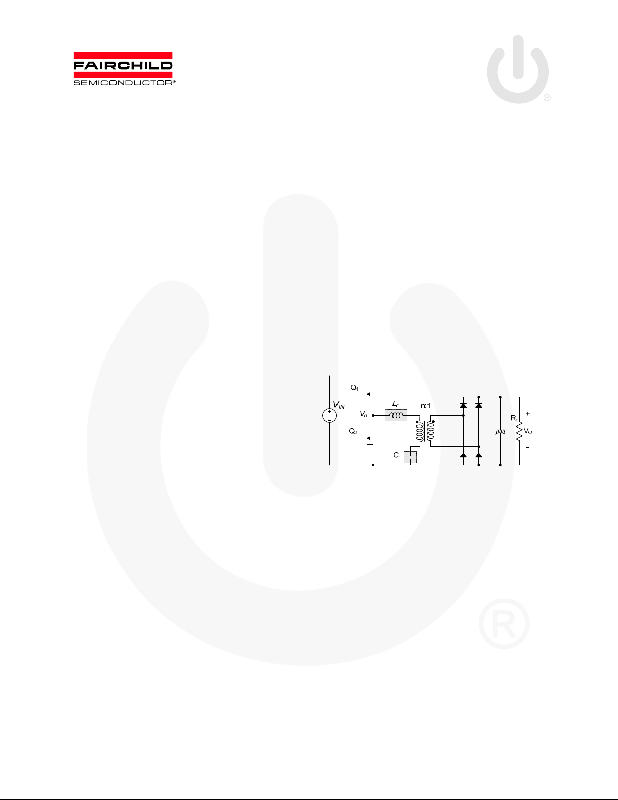
Among various kinds of resonant converters, the simplest and most popular is the LC series resonant converter, where the rectifier-load network is placed in series with the L-C resonant network, as depicted in Figure 1 configuration, the resonant network and the load act as a voltage divider. By changing the frequency of driving voltage Vd, the impedance of the resonant network changes. The input voltage is split between this impedance and the reflected load. Since it is a voltage divider, the DC gain of a LC series resonant converter is always <1. At light-load condition, the impedance of the load is large compared to the impedance of the resonant network; all the input voltage is imposed on the load. This makes it difficult to regulate the output at light load. Theoretically, frequency should be infinite to regulate the output at no load.

Figure 1. Half-Bridge, LC Series Resonant Converter

To overcome the limitation of series resonant converters, the LLC resonant converter has been proposed LLC resonant converter is a modified LC series resonant converter implemented by placing a shunt inductor across the transformer primary winding, as depicted in Figure 2. When this topology was first presented, it did not receive much attention due to the counterintuitive concept that increasing the circulating current in the primary side with a shunt inductor can be beneficial to circuit operation. However, it can be very effective in improving efficiency for high-input voltage applications where the switching loss is more dominant than the conduction loss.

In most practical designs, this shunt inductor is realized using the magnetizing inductance of the transformer. The circuit diagram of LLC resonant converter looks much the same as the LC series resonant converter: the only difference is the value of the magnetizing inductor. While the series resonant converter has a magnetizing inductance larger than the LC series resonant inductor (Lr), the magnetizing inductance in an LLC resonant converter is just 3~8 times Lr, which is usually implemented by introducing an air gap in the transformer.

[2-4].

In this

[8-12]

. The

AN-9729 APPLICATION NOTE

network even though a square-wave voltage is applied to the resonant network. The current (Ip) lags the voltage applied to the resonant network (that is, the fundamental component of the square-wave voltage (Vd) applied to the half-bridge totem pole), which allows the MOSFETs to be turned on with zero voltage. As shown in Figure 4, the MOSFET turns on while the voltage across the MOSFET is zero by

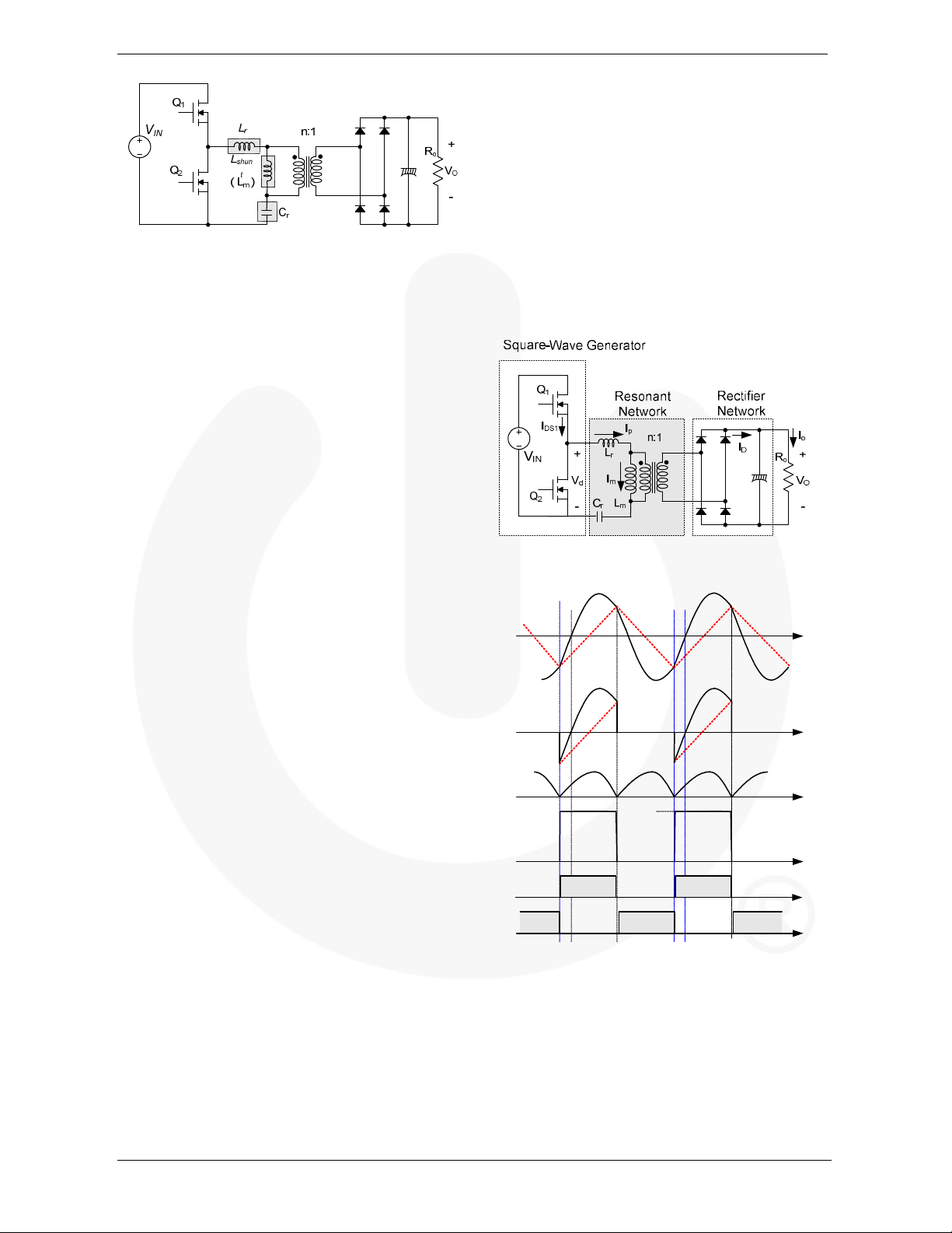
Figure 2. Half-Bridge LLC Resonant Converter

An LLC resonant converter has many advantages over a series resonant converter. It can regulate the output over wide line and load variations with a relatively small variation of switching frequency. It can achieve zero

flowing current through the anti-parallel diode.



The rectifier network produces DC voltage by rectifying the AC current with rectifier diodes and a capacitor. The rectifier network can be implemented as a full-wave bridge or center-tapped configuration with capacitive output filter.

voltage switching (ZVS) over the entire operating range. All essential parasitic elements, including junction capacitances of all semiconductor devices and the leakage inductance and magnetizing inductance of the transformer, are utilized to achieve soft switching.

This application note presents design considerations of an LLC resonant half-bridge converter employing Fairchild’s FLS-XS series. It includes explanation of the LLC resonant converter operation principles, designing the transformer and resonant network, and selecting the components. The step-by-step design procedure, explained with a design example, helps design the LLC resonant converter.

Figure 3. Schematic of Half-Bridge LLC

Resonant Converter

LLC Resonant Converter and Fundamental Approximation

Figure 3 shows a simplified schematic of a half-bridge LLC resonant converter, where Lm is the magnetizing inductance that acts as a shunt inductor, Lr is the series resonant inductor, and Cr is the resonant capacitor. Figure 4 illustrates the typical waveforms of the LLC resonant converter. It is assumed that the operation frequency is same as the resonance frequency, determined by the resonance between Lr and Cr. Since the magnetizing inductor is relatively small, a considerable amount of magnetizing current (Im) exists, which freewheels in the primary side without being involved in the power transfer. The primary-side current (Ip) is sum of the magnetizing current and the secondary-side current referred to the primary.

In general, the LLC resonant topology consists of three stages shown in Figure 3; square-wave generator, resonant network, and rectifier network.



The square-wave generator produces a square-wave voltage, Vd, by driving switches Q1 and Q2 alternately with 50% duty cycle for each switch. A small dead time is usually introduced between the consecutive transitions. The square-wave generator stage can be built as a full-bridge or half-bridge type.



The resonant network consists of a capacitor, leakage inductances, and the magnetizing inductance of the transformer. The resonant network filters the higher harmonic currents. Essentially, only sinusoidal current is allowed to flow through the resonant

I

p

I

m

I

DS1

I

D

V

IN

V

d

V

gs1

V

gs2

Figure 4. Typical Waveforms of Half-Bridge LLC

Resonant Converter

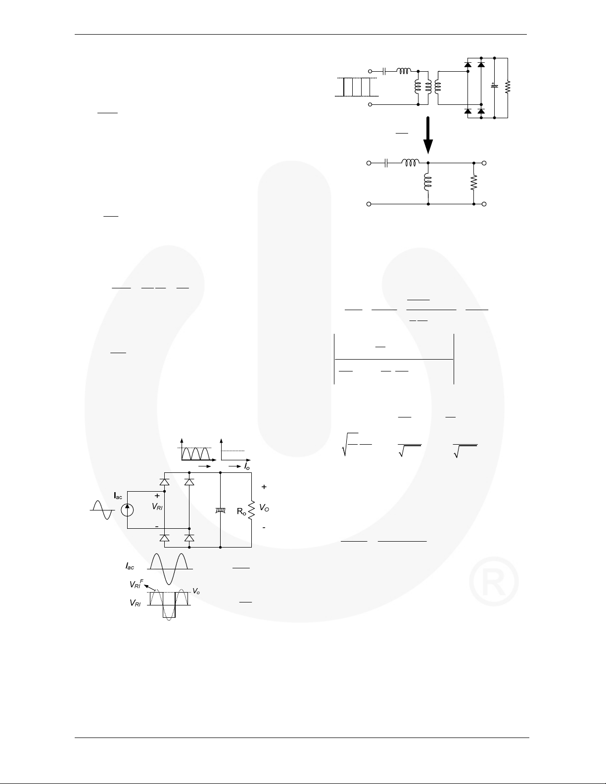
The filtering action of the resonant network allows use of the fundamental approximation to obtain the voltage gain of the resonant converter, which assumes that only the fundamental component of the square-wave voltage input to the resonant network contributes to the power transfer to the output. Because the rectifier circuit in the secondary side acts as an impedance transformer, the equivalent load resistance is different from actual load resistance. Figure 5 shows how this equivalent load resistance is derived. The

AN-9729 APPLICATION NOTE

sin( )

2

I t

π

ω

⋅

sin( ) 0

ω

= + >

= − <

sin( )

V t

ω

ac o

R R

ac o

R R

sin( )

V wt

π

⋅

π

ac o

R R

RO RI o

V n V n V

⋅

⋅ ⋅

L C L C

o

ω ω

= = = =

primary-side circuit is replaced by a sinusoidal current source, Iac, and a square wave of voltage, VRI, appears at the input to the rectifier. Since the average of |Iac| is the output current, Io, Iac, is obtained as:

I

o

=

ac

(1)

and VRI is given as:

V V if t

RI o

V V if t

RI o

ω

(2)

where Vo is the output voltage.

The fundamental component of VRI is given as:

4

V

F

o

=

RI

π

(3)

Since harmonic components of VRI are not involved in the power transfer, AC equivalent load resistance can be calculated by dividing V

F

by Iac as:

RI

F

8 8

VV

RI

= = =

I I

ac o

o

2 2

π π

(4)

Considering the transformer turns ratio (n=Np/Ns), the equivalent load resistance shown in the primary side is obtained as:

2

8

n

=

2

π

(5)

By using the equivalent load resistance, the AC equivalent circuit is obtained, as illustrated in Figure 6, where V

F

and V

d

F

are the fundamental components of

RO

the driving voltage, Vd, and reflected output voltage, VRO (nVRI), respectively.

pk

I

ac

V

IN

n=Np/N

Figure 6. AC Equivalent Circuit for LLC

With the equivalent load resistance obtained in Equation 5, the characteristics of the LLC resonant converter can be derived. Using the AC equivalent circuit of Figure 6, the voltage gain, M, is obtained as:

M

= = = =

V V V

d d in

=

2 2

ω ω ω

( 1) ( 1)( 1)

2 2

ω ω ω

p o o

where:

L L L R R m

= + = =

p m r ac o

L

Q

= = =

C R

C

r

L

V

d

+

-

s

F

V

d

r

L

m

Np:N

s

2

8

n

=

2

π

L

C

r

L

m

Resonant Converter

4

n V

o

F F

ω

2

( ) ( 1)

m

ω

o

j m Q

− + − −

8

, ,

π

1 1 1

r

, ,

ω ω

r ac

o p

sin( )

π

4

V

in

sin( )

2

π

−

2

n

2

r r p r

+

V

(nV

O

R

o

-

F

Ro

F

)

RI

+

V

RI

-

R

ac

t

ω

2

t

ω

(6)

L

p

L

r

As can be seen in Equation (6), there are two resonant frequencies. One is determined by Lr and Cr, while the other is determined by Lp and Cr.

Equation (6) shows the gain is unity at resonant frequency (ωo), regardless of the load variation, which is given as:

( 1)

m

o

− ⋅

ω ω

2

n V

M at

I

o

I

=

ac

)sin(2wt

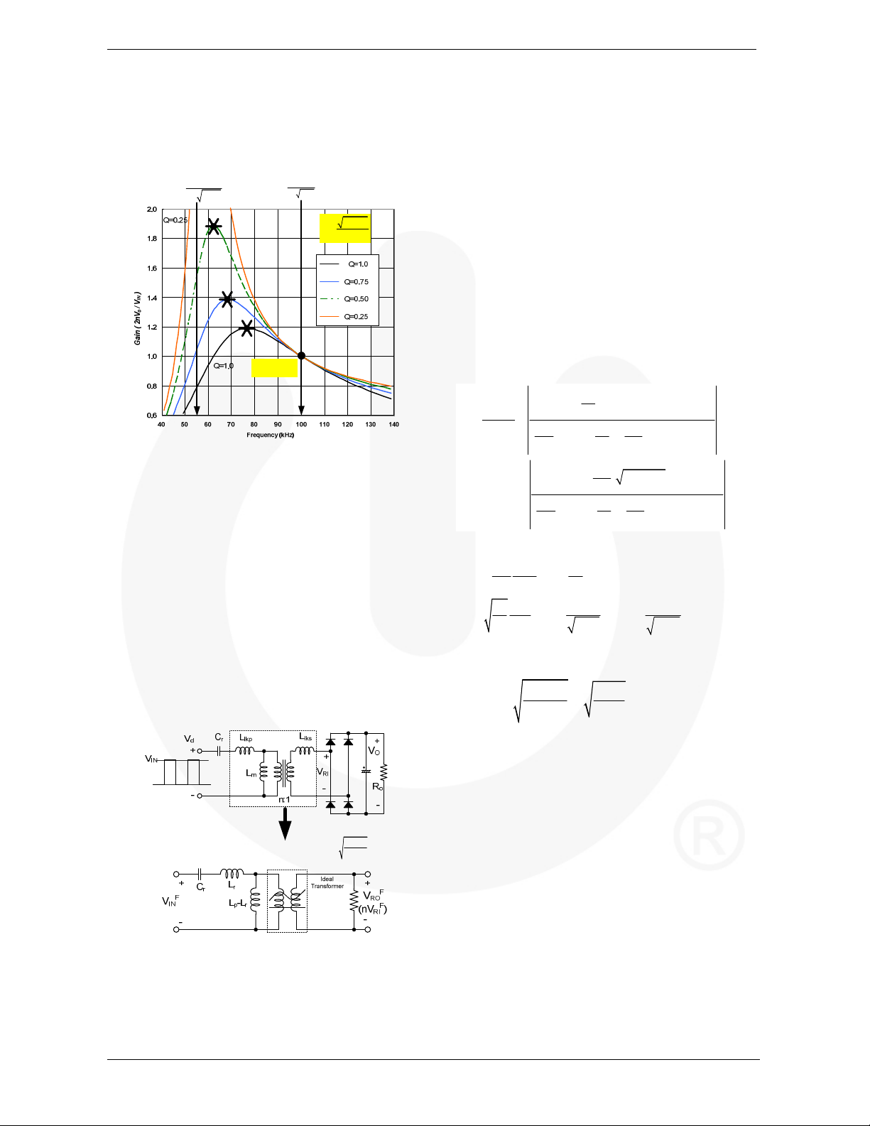
The gain of Equation (6) is plotted in Figure 7 for different Q values with m=3, fo=100kHz, and fp=57kHz.

⋅

V

in o p

ω

2 2

−

2

p

1

(7)

As observed in Figure 7, the LLC resonant converter

4

V

F

o

=

RI

Figure 5. Derivation of Equivalent Load Resistance Rac

shows gain characteristics that are almost independent of the load when the switching frequency is around the resonant frequency, fo. This is a distinct advantage of LLC-type resonant converter over the conventional series resonant converter. Therefore, it is natural to operate the converter around the resonant frequency to minimize the switching frequency variation.

The operating range of the LLC resonant converter is limited by the peak gain (attainable maximum gain), which is indicated with ‘*’ in Figure 7. Note that the peak voltage gain does not occur at fo or fp. The peak gain frequency where the peak gain is obtained exists between

AN-9729 APPLICATION NOTE

p r

L C

/

r r

L C

1

=

r r

L C

( )

p r

L L

//( )

r lkp m lks

L L L n L

p lkp m

L L L

= +

ac

R

1:VM

//( ) //

r lkp m lks lkp m lkp

L L L n L L L L

= +

e

j m Q

− + ⋅ − ⋅ − ⋅

L C L C

V o

ω ω

= = = =

fp and fo, as shown in Figure 7. As Q decreases (as load

decreases), the peak gain frequency moves to fp and higher peak gain is obtained. Meanwhile, as Q increases (as load increases), the peak gain frequency moves to fo and the peak gain drops; the full load condition should be worst case for the resonant network design.

1

f

=

p

2

π

1

f

=

o

2

π

QR=

ac

In Figure 8, the effective series inductor (Lp) and shunt inductor (Lp-Lr) are obtained by assuming n2L

lks=Llkp

and referring the secondary-side leakage inductance to the primary side as:

L L L

p m lkp

= + = +

2

(8)

When handling an actual transformer, equivalent circuit with Lp and Lr is preferred since these values can be measured with a given transformer. In an actual transformer, Lp and Lr can be measured in the primary side with the secondary-side winding open circuited and short circuited, respectively.

In Figure 9, notice that a virtual gain MV is introduced, which is caused by the secondary-side leakage inductance. By adjusting the gain equation of Equation (6) using the modified equivalent circuit of Figure 9, the gain equation

M

@

f

o

Figure 7. Typical Gain Curves of LLC Resonant

Converter (m=3)

Consideration for Integrated Transformer

For practical design, it is common to implement the magnetic components (series inductor and shunt inductor) using an integrated transformer; where the leakage inductance is used as a series inductor, while the magnetizing inductor is used as a shunt inductor. When building the magnetizing components in this way, the equivalent circuit in Figure 6 should be modified as shown in Figure 8 because leakage inductance exists, not only in the primary side, but also in the secondary side. Not considering the leakage inductance in the transformer secondary side generally results in an ineffective design.

for integrated transformer is obtained by:

ω

2

( ) ( 1)

m M

2

n V

⋅

M

O o

= =

V

in

2 2

ω ω ω

( 1) ( ) ( 1) ( 1)

− + ⋅ − ⋅ −

2 2

ω ω ω

p o o

=

2 2

ω ω ω

( 1) ( ) ( 1) ( 1)

2 2

ω ω ω

p o o

where:

2

R L

8

n

e

R m

ac

e

Q

= = =

o

= =

C R

,

2 2

M L

π

V r

1 1 1

L

r

, ,

ω ω

o p

e

r ac

⋅ − ⋅

ω

j m Q

2

ω

( ) ( 1)

2

ω

o

p

r r p r

m m

V

e

−

(9)

The gain at the resonant frequency (ωo) is fixed regardless of the load variation, which is given as:

L

M M at

p

L L m

− −

p r

m

1

(10)

The gain at the resonant frequency (ωo) is unity when using individual core for series inductor, as shown in Equation 7. However, when implementing the magnetic components with integrated transformer, the gain at the resonant frequency (ωo) is larger than unity due to the

= +

L L L

= +

lkp m lkp

2

//

L

p

M

=

V

−

virtual gain caused by the leakage inductance in the transformer secondary side.

The gain of Equation (9) is plotted in Figure 10 for different Qe values with m=3, fo=100kHz, and fp=57kHz. As observed in Figure 9, the LLC resonant converter shows gain characteristics almost independent of the load when the switching frequency is around the resonant frequency, fo.

Figure 8. Modified Equivalent Circuit to

Accommodate the Secondary-Side Leakage

Inductance

AN-9729 APPLICATION NOTE

p r

L C

/

r r

L C

f V

M M

=

r r

L C

1

2of

1

2Sf

1

f

=

p

2

π

1

f

=

o

2

π

Gain (M)

B

e

QR=

e

ac

@

o

Figure 9. Typical Gain Curves of LLC Resonant

Converter (m=3) Using an Integrated Transformer

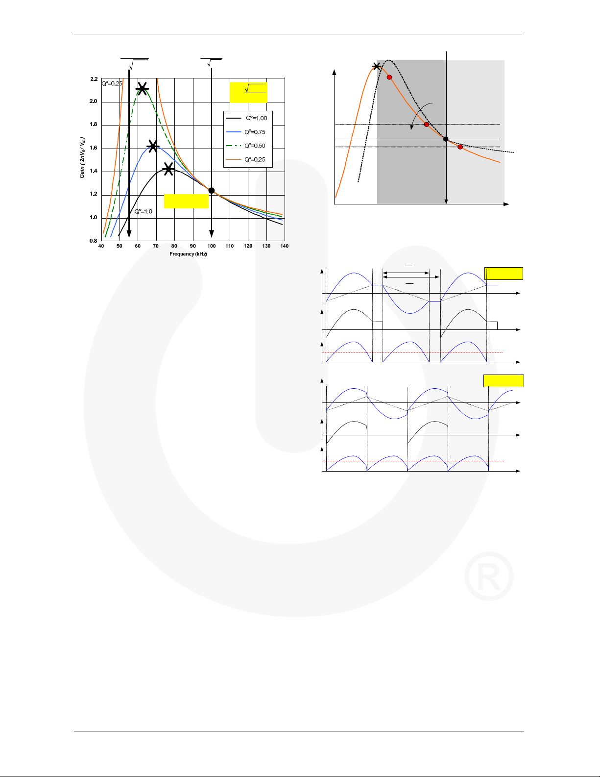
Consideration of Operation Mode and Attainable Maximum Gain

Operation Mode

The LLC resonant converter can operate at frequency below or above the resonance frequency (fo), as illustrated in Figure 10. Figure 11 shows the waveforms of the currents in the transformer primary side and secondary side for each operation mode. Operation below the resonant frequency (case I) allows the soft commutation of the rectifier diodes in the secondary side, while the circulating current is relatively large. The circulating current increases more as the operation frequency moves downward from the resonant frequency. Meanwhile, operation above the resonant frequency (case II) allows the circulating current to be minimized, but the rectifier diodes are not softly commutated. Below-resonance operation is preferred for high output voltage applications, such as street LED lighting systems where the reverserecovery loss in the rectifier diode is severe. Belowresonance operation has a narrow frequency range with respect to the load variation since the frequency is limited below the resonance frequency even at no-load condition.

On the other hand, above-resonance operation has less conduction loss than the below-resonance operation. It can show better efficiency for low output voltage applications, such as Liquid Crystal Display (LCD) TV or laptop adaptor, where Schottky diodes are available for the secondary-side rectifiers and reverse-recovery problems are insignificant. However, operation above the resonant frequency may cause too much frequency increase at light-load condition. Above-frequency operation requires frequency skipping to prevent too much increase of the switching frequency.

A

Loa d Increase

I

II

Below

Res onance

(fs<fo)

Figure 10. Operation Modes According to the

Operation Frequency

I

p

I

DS1

I

D

I

p

I

DS1

I

D

I

m

I

m

Figure 11. Waveforms of Each Operation Mode

Above

Res onance

f

o

(fs>fo)

Required Maximum Gain and Peak Gain

Above the peak gain frequency, the input impedance of the resonant network is inductive and the input current of the resonant network (Ip) lags the voltage applied to the resonant network (Vd). This permits the MOSFETs to turn on with zero voltage (ZVS), as illustrated in Figure 12. Meanwhile, the input impedance of the resonant network becomes capacitive and Ip leads Vd below the peak gain frequency. When operating in capacitive region, the MOSFET body diode is reverse recovered during the switching transition, which results in severe noise. Another problem of entering the capacitive region is that the output voltage becomes out of control since the slope of the gain is reversed. The minimum switching frequency should be limited above the peak gain frequency.

f

s

(I) fs< f

I

(II) fs> f

I

o

O

o

O

AN-9729 APPLICATION NOTE

Even though the peak gain at a given condition can be

M

Capacitive Region

Peak Gain

Inductive

Region

obtained using the gain in Equation (6), it is difficult to express the peak gain in explicit form. To simplify the analysis and design, the peak gains are obtained using simulation tools and depicted in Figure 14, which shows how the peak gain (attainable maximum gain) varies with Q for different m values. It appears that higher peak gain

f

s

V

d

V

d

can be obtained by reducing m or Q values. With a given resonant frequency (fo) and Q value, decreasing m means reducing the magnetizing inductance, which results in increased circulating current. There is a trade-off between the available gain range and conduction loss.

2.2

2.1

2

I

p

DS1

I

p

DS1

Reverse Recovery ZVS

Figure 12. Operation Waveforms for Capacitive

and Inductive Regions

The available input voltage range of the LLC resonant converter is determined by the peak voltage gain. Thus, the resonant network should be designed so that the gain curve has an enough peak gain to cover the input voltage range. However, ZVS condition is lost below the peak gain point, as depicted in Figure 12. Therefore, some margin is required when determining the maximum gain to guarantee stable ZVS operation during the load transient and startup. Typically 10~20% of the maximum gain is used as a margin, as shown in Figure 13.

Gain (M)

Peak Gain

Maximum Operation Gain

max

(M

)

10~20% of M

max

1.9

1.8

1.7

1.6

1.5

Peak Gain

1.4

1.3

1.2

m=5.0

1.1

1

0.2 0.4 0.6 0.8 1 1.2 1.4

m=9.0

0.3

0.5 0.7 0.9 1.1 1.3

m=6.0

m=7.0m=8.0

Q

m=4.5

m=4.0

m=3.5

m=2.25

m=2.5

m=3.0

Figure 14. Peak Gain (Attainable Maximum Gain)

vs. Q for Different m Values

f

o

f

s

Figure 13. Determining the Maximum Gain

AN-9729 APPLICATION NOTE

Features of FLS-XS Series

FLS-XS series is an integrated Pulse Frequency Modulation (PFM) controller and MOSFETs specifically designed for Zero Voltage Switching (ZVS) half-bridge converters with minimal external components. The internal controller includes an under-voltage lockout, optimized high-side / low-side gate driver, temperaturecompensated precise current controlled oscillator, and self-protection circuitry. Compared with discrete MOSFET and PWM controller solutions, FLS-XS series can reduce total cost, component count, size, and weight; while simultaneously increasing efficiency, productivity, and system reliability.

Figure 15. Package Diagram

Table 1. Pin Description

Pin# Name Description

1 VDL

2 AR

3 RT

4 CS

5 SG This pin is the control ground.

6 PG

7 LVCC

8 NC No connection.

9 HVCC

10 V

This pin is the drain of the high-side MOSFET, typically connected to the input DC link voltage.

This pin is for discharging the external soft-start capacitor when any protections are triggered. When the voltage of this pin drops to 0.2V, all protections are reset and the controller starts to operate again.

This pin is to program the switching frequency. Typically, opto-coupler and resistor are connected to this pin to regulate the output voltage.

This pin is to sense the current flowing through the low-side MOSFET. Typically negative voltage is applied on this pin.

This pin is the power ground. This pin is connected to the source of the lowside MOSFET.

This pin is the supply voltage of the control IC.

This pin is the supply voltage of the high-side drive circuit.

This pin is the drain of the low-side MOSFET. Typically transformer is

CTR

connected to this pin.

Figure 16. Functional Block Diagram of FSFR-Series

AN-9729 APPLICATION NOTE

o

ff

P

in O PFC

in HU

P T

400

V V V

Series

FLS-XS

Figure 17. Reference Circuit for Design Example of LLC Resonant Half-Bridge Converter

Design Procedure

In this section, a design procedure is presented using the schematic in Figure 17 as a reference. An integrated transformer with center tap, secondary side is used and input is supplied from Power Factor Correction (PFC) preregulator. A DC-DC converter with 100W/100V output has been selected as a design example. The design specifications are as follows:

 Nominal input voltage: 400VDC (output of PFC stage)  Output: 100V/1A (100W)  Hold-up time requirement: 30ms (50Hz line freq.)  DC link capacitor of PFC output: 240µF

[STEP-1] Define System Specifications

Estimated Efficiency (Eff): The power conversion efficiency must be estimated to calculate the maximum input power with a given maximum output power. If no reference data is available, use Eff = 0.88~0.92 for lowvoltage output applications and Eff = 0.92~0.96 for highvoltage output applications. With the estimated efficiency, the maximum input power is given as:

PE=

in

Input Voltage Range (V

input voltage would be the nominal PFC output voltage as:

V V=

max

min

and V

in

.

max

): The maximum

in

(11)

(12)

Even though the input voltage is regulated as constant by PFC pre-regulator, it drops during the hold-up time. The minimum input voltage considering the hold-up time requirement is given as:

min 2

V V

= −

in O PFC

where V

O.PFC

2

.

C

DL

(13)

is the nominal PFC output voltage, THU is

a hold-up time, and CDL is the DC link bulk capacitor.

(Design Example)

P

o

P

in

E

ff

max

= =

min

400

.

2

−=

in O PFC

Assuming the efficiency is 92%,

100

92.0

W

109

===

TPVV2

2

PFCOin

.

×⋅⋅

10240

×

HUin

−=

−

10301092

6

−

C

DL

3

V364

=

[STEP-2] Determine Maximum and Minimum Voltage Gains of the Resonant Network

As discussed in the previous section, it is typical to operate the LLC resonant converter around the resonant frequency (fo) to minimize switching frequency variation. Since the input of the LLC resonant converter is supplied from PFC output voltage, the converter should be designed to operate at fo for the nominal PFC output voltage.

AN-9729 APPLICATION NOTE

1

m

−

max min

1.12

min

2 2

o

n V

P

o ac

Q f R

⋅ ⋅

o r

f C

p r

L m L

= ⋅

As observed in Equation (10), the gain at fo is a function of m (m=Lp/Lr). The gain at fo is determined by choosing that

value of m. While a higher peak gain can be obtained with a small m value, too small m value results in poor coupling of the transformer and deteriorates the efficiency. It is typical to set m to be 3~7, which results in a voltage gain of 1.1~1.2 at the resonant frequency (fo).

With the chosen m value, the voltage gain for the nominal PFC output voltage is obtained as:

min

Mm=

@f=fo

(14)

[STEP-4] Calculate Equivalent Load Resistance

With the transformer turns ratio obtained from Equation (16), the equivalent load resistance is obtained as:

8

R

=

ac

(Design Example)

8

= 405

R

ac

2

π

2

n

2

+

)(

VV

Fo

=

P

o

2

⋅

ππ

⋅⋅

100

22

9.10022.28

(17)

Ω=

[STEP-5] Design the Resonant Network

With m value chosen in STEP-2, read proper Q value from

which would be the minimum gain because the nominal PFC output voltage is the maximum input voltage (V

max

in

The maximum voltage gain is given as:

max

V

M M

in

=

min

V

in

(Design Example)

(15)

The ratio (m) between Lp and Lr is chosen as 5. The minimum and maximum gains are obtained as:

V

min

M

max

M

V

in

max

V

in

min

V

in

Gain (M)

max

M

min

M

RO

max

2

min

400

364

Mm= =

5

m

=

1

−==m

=⋅== m

(Available Maximum Gain)

1.23

m

1

−

23.112.1

=

15

Peak Gain

12.1

1.12

for V

V

( V

IN

for

max

IN

O.PFC

min

)

the peak gain curves in Figure 14 that allows enough peak

).

gain. Considering the load transient and stable zerovoltage-switching (ZVS) operation, 10~20% margin should be introduced on the maximum gain when determining the peak gain. Once the Q value is determined, the resonant parameters are obtained as:

C

=

r

L

=

r

2

π

1

(2 )

π

1

2

(Design Example)

From STEP-2, the maximum voltage gain (M minimum input voltage (V

min

) is 1.23. With 15% margin, a

in

peak gain of 1.41 is required. m has been chosen as 5 in STEP-2 and Q is obtained as 0.42 from the peak gain curves in Figure 19. By selecting the resonant frequency as 100kHz, the resonant components are determined as:

C 35.9

=

r

L

r

1

2

π

1

)2(

rp

=

RofQ

⋅⋅

π

ac

==

Cf

ππ

ro

HLmL

µ

1355=⋅=

1

1010042.02

=

3

405

⋅×⋅⋅

1

9232

−

1035.9)101002(

×⋅××

=

max

) for the

nF

µ

271

(18)

(19)

(20)

H

f

o

s

Figure 18. Maximum Gain / Minimum Gain

[STEP-3] Determine the Transformer Turns Ratio (n=Np/Ns)

With the minimum gain (M transformer turns ratio is given as:

N

p

n M

= = ⋅

N V V

s o F

max

V

in

2( )

+

where VF is the secondary-side rectifier diode voltage drop.

(Design Example) assuming VF is 0.9V

N

p

n

N

s

max

V

in

== M

+

VV

min

) obtained in STEP-2, the

,

400

=⋅

min

)(2

FO

)9.0100(2

+

(16)

Figure 19. Resonant Network Design Using the Peak Gain

(Attainable Maximum Gain) Curve for m=5

22.212.1

=⋅

AN-9729 APPLICATION NOTE

s V e

f M B A

+

⋅ ⋅ ∆ ⋅

B

∆

min

10

10711.14.01080

2

[STEP-6] Design the Transformer

The worst case for the transformer design is the minimum switching frequency condition, which occurs at the minimum input voltage and full-load condition. To obtain the minimum switching frequency, plot the gain curve using gain Equation 9 and read the minimum switching frequency. The minimum number of turns for the transformer primary-side is obtained as:

( )

min

N

p

n V V

min

o F

=

2

(21)

where Ae is the cross-sectional area of the transformer core in m2 and ∆B is the maximum flux density swing in Tesla, as shown in Figure 20. If there is no reference data, use ∆B =0.3~0.4 T.

V

1/(2fs)

RI

n (Vo+VF)/M

V

Figure 21. Gain Curve

[STEP-7] Transformer Construction

Parameters Lp and Lr of the transformer were determined in

-n (Vo+VF)/M

V

B

Figure 20. Flux Density Swing

Choose the proper number of turns for the secondary side that results in primary-side turns larger than N

N n N N= ⋅ >

p s p

(Design Example)

EER3542 core (Ae=107mm2) is selected for the transformer. From the gain curve of Figure 21, the minimum switching frequency is obtained as 70KHz. The minimum primary-side turns of the transformer is given as:

VVn

+

min

N

=

p

min

=

)(

Fo

ABf

⋅⋅∆

11.12

es

9.10022.2

×

=

63

−

×⋅⋅⋅××

Choose Ns so that the resultant Np is larger than N

min

291322.2

NNnN

<=×=⋅=

psp

min

311422.2

NNnN

>=×=⋅=

psp

min

331522.2

NNnN

>=×=⋅=

361622.2

>=×=⋅=

381722.2

>=×=⋅=

psp

min

NNnN

psp

min

NNnN

psp

min

as:

p

(22)

turns 30

min

:

p

STEP-5. Lp and Lr can be measured in the primary side with the secondary-side winding open circuited and short circuited, respectively. Since LLC converter design requires a relatively large Lr, a sectional bobbin is typically used, as shown in Figure 22, to obtain the desired Lr value. For a sectional bobbin, the number of turns and winding configuration are the major factors determining the value of Lr, while the gap length of the core does not affect Lr much. Lp can be controlled by adjusting the gap length. Table 2 shows measured Lp and Lr values with different gap lengths. A gap length of 0.05mm obtains values for Lp and Lr closest to the designed parameters.

N p

Figure 22. Sectional Bobbin

Table 2.

Measured Lp and Lr with Different Gap Lengths

Gap Length Lp Lr

0.0mm 2,295µH 123µH

0.05mm 943µH 122µH

0.10mm 630µH 118µH

0.15mm 488µH 117µH

0.20mm 419µH 115µH

0.25mm 366µH 114µH

N

s2

N

s1

AN-9729 APPLICATION NOTE

2 2

[ ] [ ]

2 2 4 2 ( )

2( )

D o F

V V V

= +

4

D o

I I

π

8

Co o o

I I I

(Design Example)

Final Resonant Network Design

Even though the integrated transformer approach in LLC resonant converter design can implement the magnetic components in a single core and save one magnetic component, the value of Lr is not easy to control in real transformer design. Resonant network design sometimes requires iteration with a resultant Lr value after the transformer is built. The resonant capacitor value is also changed since it should be selected among off-the-shelf capacitors. The final resonant network design is summarized in Table 3 and the new gain curves are shown in Figure 23.

Table 3.

Final Resonant Network Design Parameters

Parameters Initial Design Final Design

Lp 1365µH

Lr 273H

Cr 9.3nF

fo 100kHz

m 5

Q 0.42 0.26

M@fo 1.12

Minimum

Frequency

80kHz

850µH

170µH

15nF

99.7kHz

5

1.12

80kHz

Gain

The nominal voltage of the resonant capacitor in normal operation is given as:

V

nom

C

r

max

V I

in Cr

≅ +

2 2

2

⋅

f C

π

⋅ ⋅ ⋅

RMS

o r

(24)

However, the resonant capacitor voltage increases much higher at overload condition or load transient. Actual capacitor selection should be based on the Over-Current Protection (OCP) trip point. With the OCP level, I

OCP

, the

maximum resonant capacitor voltage is obtained as:

max

V I

nom

V

C

r

(Design Example)

RMS

I

C

r

1

=

92.0

in OCP

≅ +

2 2

1

[

E

ff

1

⋅

π

[

22.222

⋅

I

π

⋅ ⋅ ⋅

22

n

[2]

+

f C

o r

[]

+≅

)(

VVn

+

FoO

LLMf

−

)9.0100(22.2

+

3

109924

(25)

22

]

)(24

rpvo

2

]

6

−

1068012.1

×⋅⋅×⋅

=0.78A

The peak current in the primary side in normal operation is:

peak

C

OCP level is set to 1.75A with 50% margin on I

nom

V

C

r

400

+=

2

max

V

C

r

400

+=

2

rms

C

rr

max

V

in

+≅

2

⋅

π

max

+≅

22

75.1

π

AII

103.12 =⋅=

peak

:

RMS

I

⋅

2

C

r

Cf

⋅⋅⋅

π

ro

78.02

101510992

×⋅×⋅⋅

IV

OCPin

Cf

⋅⋅⋅

π

101510992

×⋅×⋅⋅

V318

=

93

−

ro

V7.387

=

93

−

Cr

A 630V rated low-ESR film capacitor is selected for the resonant capacitor.

Figure 23. Gain Curve of the Final Resonant

[STEP-8] Select the Resonant Capacitor

When choosing the resonant capacitor, the current rating should be considered because a considerable amount of current flows through the capacitor. The RMS current through the resonant capacitor is given as:

1 ( )

RMS

I

≅ +

C

r

E

ff

Network Design

I n V V

π

o o F

n f M L L

o V p r

[STEP-9] Rectifier Network Design

When the center tap winding is used in the transformer

+

−

secondary side, the diode voltage stress is twice of the output voltage expressed as:

The RMS value of the current flowing through each rectifier diode is given as:

RMS

=

Meanwhile, the ripple current flowing through output capacitor is given as:

(23)

I

RMS

π π

o

( )

= − =

2 2

2

−

8

(26)

(27)

(28)

AN-9729 APPLICATION NOTE

2

o o C

V I R

π

∆ = ⋅

Loss Co Co C

P I R

= ⋅

=+=+=

100( )

f kHz

Ω

( ) 100 ( )

f kHz

Ω Ω

( ) 100 40 ( )

f kHz

Ω Ω

SS SS SS

T times of R C

= ⋅

The voltage ripple of the output capacitor is:

(29)

where RC is the effective series resistance (ESR) of the output capacitor and the power dissipation is the output capacitor is:

2

RMS

( )

.

(Design Example)

(30)

The voltage stress and current stress of

the rectifier diode are:

VVVV

FoD

π

RMS

D

o

AII

785.04==

8.201)9.0100(2)(2

The 600V/8A Ultra fast recovery diode is selected for the rectifier, considering the voltage overshoot caused by the stray inductance.

The RMS current of the output capacitor is:

I

RMS

I

C

o

π

2

o

)

(

22

2

8

−

π

2

=−=

8

AII

48.0

=

oo

When two electrolytic capacitors with ESR of 100mΩ are used in parallel, the output voltage ripple is given as:

1.0

ππ

Coo

(1

2

22

VRIV

079.0)

=⋅⋅=⋅=∆

The loss in electrolytic capacitors is:

RMS

CCLoss

,

oo

22

C

WRIP

01.005.048.0)(

==⋅=⋅=

Figure 24. Typical Circuit Configuration for RT Pin

Soft-Start To prevent excessive inrush current and overshoot of output voltage during startup, increase the voltage gain of the resonant converter progressively. Since the voltage gain of the resonant converter is reversely proportional to the switching frequency, soft-start is implemented by sweeping down the switching frequency from an initial high frequency (f

ISS

) until the output voltage is established, as illustrated in Figure 25. The soft-start circuit is made by connecting RC series network on the RT pin as shown in Figure 24. FLS-XS series also has an internal soft-start for 3ms to reduce the current overshoot during the initial cycles, which adds 40KHz to the initial frequency of the external soft-start circuit, as shown in Figure 25. The actual initial frequency of the soft-start is given as:

[STEP-10] Control Circuit Configuration

Figure 24 shows the typical circuit configuration for the RT pin of FLS-XS series, where the opto-coupler transistor is connected to the RT pin to control the switching frequency. The minimum switching frequency occurs when the optocoupler transistor is fully tuned off, which is given as:

5.2

k

= ×

min

R

min

Assuming the saturation voltage of the opto-coupler transistor is 0.2V, the maximum switching frequency is determined as:

5.2 4.68

k k

= + ×

max

R R

min max

(31)

(32)

5.2 5.2

ISS

It is typical to set the initial frequency of soft-start (f

k k

= + × +

R R

min

SS

ISS

(33)

) as

2~3 times of the resonant frequency (fo).

The soft-start time is determined by the RC time constant:

3 ~ 4

Figure 25. Frequency Sweep of the Soft-Start

(34)

AN-9729 APPLICATION NOTE

×

(Design Example)

STEP-6. R

R 5.62.5

min

100

f

min

KHz

Considering the output voltage overshoot during transient

The minimum frequency is 80kHz in

is determined as:

Ω=Ω×= KK

(Design Example)

Since the OCP level is determined as

1.75A in STEP-8 and the OCP threshold voltage is -0.6V, a sensing resistor of 0.33Ω is used. The RC time constant is set to 100ns (1/100 of switching period) with 1kΩ resistor and 100pF capacitor.

(10%) and the controllability of the feedback loop, the maximum frequency is set as 140kHz. R

68.4

K

R

=

max

f

o

(

100

= K

×

KHz

(

KHz

100

×

KHz

68.4

Ω

40.1

−

Ω

K

40.199

−

2.5

K

Ω

)

R

min

8.7

Ω

K

2.5 )

Ω

K

5.6

is determined as:

max

Ω=

Setting the initial frequency of soft-start as 250kHz (2.5 times of the resonant frequency), the soft-start resistor RSS is given as:

2.5

K

R

=

SS

ISS

(

100

= K

(

100

−

KHz

−

40

KHz

40250

Ω

KHzf

−

Ω

K

2.5

KHzKHz

−

2.5

K

Ω

)

R

min

Ω=

4

Ω

K

2.5 )

Ω

K

5.6

[STEP-11] Current Sensing and Protection

FLS-XS series senses low-side MOSFET drain current as a negative voltage, as shown in Figure 26 and Figure 27. Half-wave sensing allows low-power dissipation in the sensing resistor, while full-wave sensing has less switching noise in the sensing signal. Typically, RC low-pass filter is used to filter out the switching noise in the sensing signal. The RC time constant of the low-pass filter should be 1/100~1/20 of the switching period.

C

r

Np

Ns

Control

IC

V

CS

SG PG

R

sense

I

DS

Ns

I

DS

V

CS

[STEP-12] Voltage and Current Feedback

Power supplies for LED lighting must be controlled by Constant Current (CC) Mode as well as a Constant Voltage (CV) Mode. Because the forward-voltage drop of LED varies with the junction temperature and the current also increases greatly consequently, devices can be damaged. Figure 28 shows an example of a CC and CV Mode feedback circuit for single output LED power supply. During normal operation, CC Mode is dominant and CV control circuit does not activate as long as the feedback voltage is lower than reference voltage, which means that CV control circuit only acts as OVP for abnormal modes.

(Design Example)

design target. VO is determined as:

V +=

o

Set the upper-side feedback resistance (RFU) as 330KΩ. RFL is determined as:

5.2

= K

R

FL

−

V

o

The output voltage of op-amp is given as:

V

sense

R

0

=

V

OC

sC

Actually, the V resistors have the same value for simplification;

V −

−=

The output voltage of the op-amp for CC control keeps zero voltage as long as the sensing voltages are lower than the reference voltage.

The output voltage (VO) is 100V in

R

FU

)1(5.2

R

FL

R

1

201

FU

=

)5.2(

V

REF

203201

R

1

203

RR

V

1

sense

(

201

R

has a negative value and assume all

sense

1

201

RsC

×

Ω×

K

3305.2

−

201

46.8

)5.2100(

VsC

⋅++

OC

201

sC

++

V

REF

)

+−=

203201

R

)(

VV

REFsenseOC

Ω=

Figure 26. Half-Wave Sensing

Figure 27. Full-Wave Sensing

Figure 28. Example of CC and CV Feedback Circuit

AN-9729 APPLICATION NOTE

×

=

Figure 29 shows another example of a CC and OverVoltage Regulation (OVR) Mode feedback circuit for multi-output LED power supply. The FAN7346 is a LED current-balance controller that controls four LED arrays to maintain equal LED current. To prevent LED driving voltage being over the withstanding voltage of component, the FAN7346 controls LED driving voltage. The OVR control circuit activates when the ENA pin is in HIGH state. If OVR pin voltage is lower than 1.5V, the Feedback Control (FB) pin voltage follows headroom control to maintain minimum voltage of drain voltages as 1V. If OVR pin voltage is higher than 1.5V, the FAN7346 controls FB (FB is pulled LOW) through FB regulation so the OVR pin voltage is not over 1.5V.

LED current is controlled by FBx pin voltage. The external current balance switch is operating in linear region to control LED current. Sensed voltage at the FBx pin is compared with internal reference voltage and controller

stress problems in the other channel. OLP function has auto-recovery: As soon as drain voltage is higher than

0.3V, OLP is finished and drain voltage feedback system is restored.

To sense over-current condition, the FAN7346 monitors FBx pin voltage. If FBx voltage is higher than 1V for 20µs, CHx is considered in over-current condition. After sensing OCP condition, individual channel switch is latched off. So, even if a channel is in OCP condition, other channels keep operating. Any OCP channel is restarted after UVLO is reset.

(Design Example)

The output voltage (VO) is 100V in

design target. VO is determined as:

V

o

+=

10

R

8

R

)

1(5.1

Set the upper-side feedback resistance (R8) as 1MΩ. R10 is determined as:

signals the gate (or base) for external current balance switch. Internal reference voltage is made from ADIM voltage. The LED current is determined as:

V

10

ADIM

R

SENSE

(35)

I×=

LED

ADIM voltage is clamped internally from 0.5V to 4V. The protections; such as open LED Protection (OLP), Short LED Protection (SLP), and Over-Current Protection (OCP); which increase system reliability, are applied in individual string protection method.

To sense a short LED condition, the FAN7346 senses drain voltage level. If LEDs are shorted, the LED forward voltage is lower than other LED strings, so its drain voltage of external balance switch is higher than other drain voltage. The SLP condition detection threshold voltage can be programmed by SLPR voltage. The internal short LED protection reference is determined as:

VV

10

_

SLPRTHSLP

(36)

Minimum SLP threshold voltage is 0V and maximum SLP threshold voltage is 45V. If any string is in SLP condition, SLP string is turned off and other string is operated normally. If the sensed drain voltage (CHx voltage) is higher than the programmed threshold voltage for 20µs, CHx goes to short LED protection. As soon as encountering SLP, the corresponding channel is forced off.

To sense an open LED condition, the FAN7346 senses drain voltage level. If LED string is opened, its drain voltage of external balance switch is grounded, so the FAN7346 detects the open-LED condition. The detection threshold voltage is 0.3V. If CHx voltage is lower than

×

R

85.1

= K

R

10

V

=

−

)5.1(

o

The output channel current (I Setting the V

ADIM

determined as:

SENSE

×

10 mA

I

V

ADIM

= 6.1

R

Choose the sense resistor (R29, R30, R31, and R32) is

1.5Ω, the OCP level is determined as:

V

THOCP

I

OCP

V

LED

RS21 RS24

RS20

CS12

RS28

_

R

SENSE

CS6

RS12

PC101

RS22

RS18

RS17

RS15

RS14

RS19 RS27

RS13 CS 9

CS14

CS15

CS8

Ω×

M

15.1

−

)5.1100(

Ω=

23.15

) is 250mA in design target.

LED

is above 4V, the current sense R

4

LED

V

=

×

25010

V

1

666

=

==

5.1

Ω

mA

Ω=

RS8

RS10

OVR

REF

CH1

RS11

FB

PWM1

PWM2

PWM3

PWM4

PWM5

ENA

SLPR

ADIM

CMP

OUT3

OUT4

OUT1

OUT2

CH4

FB4

GND

FB1

CH2

FB2

CH3

FB3

V

DD

V

CC

Q1

RS16

RS23

RS25

CS7

V

CC

Q2

CS10

CS11

RS30

RS29

Q3

RS31

SENSE

CS13

is

0.3V for 20µs, its drain voltage feedback is pulled up to 5V. This means the opened LED string is eliminated from drain feedback loop. Without OLP, minimum drain voltage

Figure 29. Example of CC and OVR Feedback Circuit

is 0V, so drain voltage feedback forces the FB signal to increase output power. This can cause SLP or thermal

Q4

RS32

AN-9729 APPLICATION NOTE

Design Summary

Figure 30 and Figure 31 show the final schematic of the LLC resonant half-bridge converter for LED lighting

Figure 30. Final Schematic of Half-Bridge LLC Resonant Converter for Single Channel

design example. EER3543 core with sectional bobbin is used for the transformer. Efficiency at full-load is around 94%.

CS7

RS11

OVR

CH1

OUT1

V

Series

FLS-XS

CC

PWM5

RS14

FB1

PWM4

PWM3

PWM2

RS15

RS17

RS18

CS10

RS16

RS29

CH2

OUT2

FB2

PWM1

VMIN

REF

RS22

CS11

RS23

RS30

CH3

OUT3

FB3

ENA

FB

Figure 31. Final Schematic of Half-Bridge LLC Resonant Converter for Multi Channel

RS32

CS13

RS25

RS31

FAN7346

CH4

GND

OUT4

FB4

SLPR

ADIM

AN-9729 APPLICATION NOTE

DS

LOAD

OP_CC

VCR [200V/div]

300V

Experimental Verification

To show the validity of the design procedure presented in this application note, the converter of the design example was built and tested. All the circuit components are used as designed in the design example.

V

Figure 32 and Figure 33 show the operation waveforms at full-load and no-load conditions for nominal input voltage. As observed, the MOSFET drain-to-source voltage (VDS) drops to zero by resonance before the MOSFET is turned on and zero voltage switching is achieved.

Figure 34 shows the waveforms of the resonant capacitor voltage and primary-side current at full-load condition. The peak values of the resonant capacitor voltage and primaryside current are 300V and 1.1A, respectively, which are well matched with the calculated values in STEP-8 of design procedure section.

Figure 35 shows the rectifier diode voltage and current waveforms at full-load condition. Due to the voltage overshoot caused by stray inductance, the voltage stress is a little bit higher than the value calculated in STEP-9.

Figure 36 shows the output load current and output voltage of op-amp waveforms for constant-current control when output load is step changed from 140mA to 1000mA at t0.

Figure 37 shows the operation waveform when LED string is opened and restored condition

IP [1A/div]

[200V/div]

IP [1A/div]

1.1A

Time (5µs/div)

Figure 34. Resonant Capacitor Voltage and Primary-

Side Current Waveforms at Full-Load Condition

IP [1A/div]

ID [1A/div]

VD [100V/div]

257V

Time (5µs/div)

Figure 35. Rectifier Diode Voltage and Current

Waveforms at Full-Load Condition

IDS [1A/div]

VDS [200V/div]

Time (5µs/div)

Figure 32. Operation Waveforms at Full-Load Condition

IP [2A/div]

IDS [1A/div]

VDS [200V/div]

Time (5µs/div)

Figure 33. Operation Waveforms at No-Load Condition

V

[2V/div]

1000mA

140mA

I

[0.5A/div]

Transient Mode

t0

Time (50ms/div)

CC Mode

t1

Figure 36. Soft-Start Waveforms

V

LED

[100V/div]

Open LED Restore LED

I

LED_OPEN

[200mA/div]

V

DS_NORMAL_LED

[500mV/div]

V

DSD_OPEN_LED

[500mV/div]

Figure 37. Open LED Protection Operation

AN-9729 APPLICATION NOTE

References

[1] Robert L. Steigerwald, “A Comparison of Half-bridge

resonant converter topologies,” IEEE Transactions on Power Electronics, Vol. 3, No. 2, April 1988.

[2] A. F. Witulski and R. W. Erickson, “Design of the series

resonant converter for minimum stress,” IEEE Transactions on Aerosp. Electron. Syst., Vol. AES-22, pp. 356-363, July 1986.

[3] R. Oruganti, J. Yang, and F.C. Lee, “Implementation of

Optimal Trajectory Control of Series Resonant Converters,” Proc. IEEE PESC ’87, 1987.

[4] V. Vorperian and S. Cuk, “A Complete DC Analysis of the

Series Resonant Converter,” Proc. IEEE PESC’82, 1982.

[5] Y. G. Kang, A. K. Upadhyay, D. L. Stephens, “Analysis and

design of a half-bridge parallel resonant converter operating above resonance,” IEEE Transactions on Industry Applications, Vol. 27, March-April 1991, pp. 386 – 395.

[6] R. Oruganti, J. Yang, and F.C. Lee, “State Plane Analysis of

Parallel Resonant Converters,” Proc. IEEE PESC ’85, 1985.

This application note written based on Fairchild Semiconductor Application Note AN-4137.

[7] M. Emsermann, “An Approximate Steady State and Small

Signal Analysis of the Parallel Resonant Converter Running Above Resonance,” Proc. Power Electronics and Variable Speed Drives ’91, 1991, pp. 9-14.

[8] Yan Liang, Wenduo Liu, Bing Lu, van Wyk, J.D, “Design

of integrated passive component for a 1MHz 1kW halfbridge LLC resonant converter,” IAS 2005, pp. 2223-2228.

[9] B. Yang, F.C. Lee, M. Concannon, “Over-current protection

methods for LLC resonant converter” APEC 2003, pp. 605 - 609.

[10] Yilei Gu, Zhengyu Lu, Lijun Hang, Zhaoming Qian,

Guisong Huang, “Three-level LLC series resonant DC/DC converter,” IEEE Transactions on Power Electronics Vol.20, July 2005, pp.781 – 789.

[11] Bo Yang, Lee, F.C, A.J Zhang, Guisong Huang, “LLC

resonant converter for front-end DC/DC conversion,” APEC

2002. pp.1108 – 1112.

[12] Bing Lu, Wenduo Liu, Yan Liang, Fred C. Lee, Jacobus D.

Van Wyk, “Optimal design methodology for LLC Resonant Converter,” APEC, 2006, pp.533-538.

Related Datasheets

FLS1800XS — Half-Bridge LLC Resonant Control IC for Lighting

FLS2100XS — Half-Bridge LLC Resonant Control IC for Lighting

FAN7346 — 4-Channel LED Current Balance Control IC

DISCLAIMER FAIRCHILD SEMICONDUCTOR RESERVES THE RIGHT TO MAKE CHANGES WITHOUT FURTHER NOTICE TO ANY PRODUCTS HEREIN TO IMPROVE RELIABILITY, FUNCTION, OR DESIGN. FAIRCHILD DOES NOT ASSUME ANY LIABILITY ARISING OUT OF THE APPLICATION OR USE OF ANY PRODUCT OR CIRCUIT DESCRIBED HEREIN; NEITHER DOES IT CONVEY ANY LICENSE UNDER ITS PATENT RIGHTS, NOR THE RIGHTS OF OTHERS.

LIFE SUPPORT POLICY FAIRCHILD’S PRODUCTS ARE NOT AUTHORIZED FOR USE AS CRITICAL COMPONENTS IN LIFE SUPPORT DEVICES OR SYSTEMS WITHOUT THE EXPRESS WRITTEN APPROVAL OF THE PRESIDENT OF FAIRCHILD SEMICONDUCTOR CORPORATION. As used herein:

1. Life support devices or systems are devices or systems which, (a) are intended for surgical implant into the body, or (b) support or sustain life, or (c) whose failure to perform when properly used in accordance with instructions for use provided in the labeling, can be reasonably expected to result in significant injury to the user.

2. A critical component is any component of a life support device or system whose failure to perform can be reasonably expected to cause the failure of the life support device or system, or to affect its safety or effectiveness.

Fairchild AN-9729 service manual

Specifications and Main Features

Frequently Asked Questions

User Manual