Ericsson AXE 2 Service Manual

Competence Development Centre

AXE Operation & Maintenance Platform

Exchange Data



Help Exit

PREFACE

Target Audience

This book is preliminary intended to be used as a course manual in the
Ericsson Operation and Maintenance training program. The book is a
training document and is not to be considered as a specification of any
Ericsson language or system.

Identification

EN/LZT 101 105/2 R1A

Responsibility

Training Supply
ETX/TK/ZM

 Ericsson Telecom AB 1996, Stockholm, Sweden

All rights reserved. No part of this document may be reproduced in any
form without the written permission of the copyright holder.

Table of Contents

1. Introduction 3

1.1 Module Objectives . . . . . . . . . . . . . . . . . . . . . . . . . . . . . . . . . . . . . 3

1.2 General . . . . . . . . . . . . . . . . . . . . . . . . . . . . . . . . . . . . . . . . . . . . . 3

2. Device and Route Data 5

2.1 Route Concepts and Definition . . . . . . . . . . . . . . . . . . . . . . . . . . . 5

2.1.1 General . . . . . . . . . . . . . . . . . . . . . . . . . . . . . . . . . . . . . . . . . . . . . 5

2.1.2 Definition of Regional Processors . . . . . . . . . . . . . . . . . . . . . . . . . 5

2.1.3 Definition of Extension Modules . . . . . . . . . . . . . . . . . . . . . . . . . . 9

2.1.4 Definition of Routes . . . . . . . . . . . . . . . . . . . . . . . . . . . . . . . . . . . 10

2.1.5 Connection of Devices to the Route . . . . . . . . . . . . . . . . . . . . . . 14

2.1.6 Printout of Device and Route Data . . . . . . . . . . . . . . . . . . . . . . . 16

2.2 Supervision Data for Trunks. . . . . . . . . . . . . . . . . . . . . . . . . . . . . 19

2.2.1 General Principles of Supervision . . . . . . . . . . . . . . . . . . . . . . . . 19

2.2.2 Blocking Supervision . . . . . . . . . . . . . . . . . . . . . . . . . . . . . . . . . . 20

2.2.3 Disturbance Supervision of Devices . . . . . . . . . . . . . . . . . . . . . . 23

2.2.4 Disturbance Supervision of Routes . . . . . . . . . . . . . . . . . . . . . . . 25

2.2.5 Seizure Quality Supervision of Devices. . . . . . . . . . . . . . . . . . . . 26

2.2.6 Groups for Seizure Quality Supervision. . . . . . . . . . . . . . . . . . . . 27

2.2.7 Seizure Supervision of Trunks. . . . . . . . . . . . . . . . . . . . . . . . . . . 28

2.3 Chapter Summary . . . . . . . . . . . . . . . . . . . . . . . . . . . . . . . . . . . . 30

3. Connection to Group Switch 31

3.1 GSS in General . . . . . . . . . . . . . . . . . . . . . . . . . . . . . . . . . . . . . . 31

3.1.1 Basic Functions, Hardware and Software.. . . . . . . . . . . . . . . . . . 31

3.1.2 Hardware Structure and Switching . . . . . . . . . . . . . . . . . . . . . . . 36

3.1.3 Control of the Switching. . . . . . . . . . . . . . . . . . . . . . . . . . . . . . . . 39

3.1.4 Security . . . . . . . . . . . . . . . . . . . . . . . . . . . . . . . . . . . . . . . . . . . . 42

3.1.5 Synchronization. . . . . . . . . . . . . . . . . . . . . . . . . . . . . . . . . . . . . . 43

3.1.6 Printouts. . . . . . . . . . . . . . . . . . . . . . . . . . . . . . . . . . . . . . . . . . . . 46

3.1.7 Blocking of Units . . . . . . . . . . . . . . . . . . . . . . . . . . . . . . . . . . . . . 47

3.2 Connection of SNT and DIP . . . . . . . . . . . . . . . . . . . . . . . . . . . . 48

i

AXE 10, Operation & Maintenance, Platform

3.2.1 General . . . . . . . . . . . . . . . . . . . . . . . . . . . . . . . . . . . . . . . . . . . . 48

3.2.2 Devices Connected to the Group Switch. . . . . . . . . . . . . . . . . . . 49

3.2.3 ETC (Exchange Terminal Circuit) . . . . . . . . . . . . . . . . . . . . . . . . 49

3.2.4 PCD (Pulse Code Device) . . . . . . . . . . . . . . . . . . . . . . . . . . . . . . 52

3.3 The SNT Concept . . . . . . . . . . . . . . . . . . . . . . . . . . . . . . . . . . . . 53

3.3.1 Connection of SNT . . . . . . . . . . . . . . . . . . . . . . . . . . . . . . . . . . . 53

3.3.2 Connection of Devices to the SNT. . . . . . . . . . . . . . . . . . . . . . . . 55

3.4 The DIP Concept. . . . . . . . . . . . . . . . . . . . . . . . . . . . . . . . . . . . . 57

3.5 Chapter Summary . . . . . . . . . . . . . . . . . . . . . . . . . . . . . . . . . . . . 62

3.6 Appendix 1. . . . . . . . . . . . . . . . . . . . . . . . . . . . . . . . . . . . . . . . . . 63

3.6.1 Channel Associated Signalling, CAS. . . . . . . . . . . . . . . . . . . . . . 63

3.6.2 Common Channel Signalling, CCS . . . . . . . . . . . . . . . . . . . . . . . 64

3.6.3 Supervision of the PCM Line. . . . . . . . . . . . . . . . . . . . . . . . . . . . 64

4. Size Alteration 67

4.1 Size Alteration . . . . . . . . . . . . . . . . . . . . . . . . . . . . . . . . . . . . . . . 67

4.1.1 Introduction . . . . . . . . . . . . . . . . . . . . . . . . . . . . . . . . . . . . . . . . . 67

4.1.2 Initial Setting . . . . . . . . . . . . . . . . . . . . . . . . . . . . . . . . . . . . . . . . 68

4.1.3 Hardware Extension . . . . . . . . . . . . . . . . . . . . . . . . . . . . . . . . . . 70

4.1.4 Extension by Using More Software Individuals . . . . . . . . . . . . . . 71

4.1.5 What is a Data File? . . . . . . . . . . . . . . . . . . . . . . . . . . . . . . . . . . 72

4.1.6 The Use of Size Alteration Events. . . . . . . . . . . . . . . . . . . . . . . . 73

4.1.7 Commands Related to Size Alteration. . . . . . . . . . . . . . . . . . . . . 74

4.2 Chapter Summary . . . . . . . . . . . . . . . . . . . . . . . . . . . . . . . . . . . . 76

5. Analysis 77

5.1 Analysis in General . . . . . . . . . . . . . . . . . . . . . . . . . . . . . . . . . . . 77

5.1.1 The Use of Operating and Non-Operating Area . . . . . . . . . . . . . 78

5.2 Branching. . . . . . . . . . . . . . . . . . . . . . . . . . . . . . . . . . . . . . . . . . . 80

5.3 Route Analysis. . . . . . . . . . . . . . . . . . . . . . . . . . . . . . . . . . . . . . . 81

5.3.1 The Sending Program . . . . . . . . . . . . . . . . . . . . . . . . . . . . . . . . . 83

5.3.2 The Commands Used to Define Routing Cases . . . . . . . . . . . . . 85

5.4 Charging Analysis . . . . . . . . . . . . . . . . . . . . . . . . . . . . . . . . . . . . 86

5.4.1 Charging Principle . . . . . . . . . . . . . . . . . . . . . . . . . . . . . . . . . . . . 86

5.4.2 Charging Method. . . . . . . . . . . . . . . . . . . . . . . . . . . . . . . . . . . . . 88

5.4.3 A Survey of the Charging Analysis . . . . . . . . . . . . . . . . . . . . . . . 89

5.4.4 Definition of Tariffs. . . . . . . . . . . . . . . . . . . . . . . . . . . . . . . . . . . . 90

5.4.5 Definition of Tariff Class. . . . . . . . . . . . . . . . . . . . . . . . . . . . . . . . 92

5.4.6 Definition of Charging Case. . . . . . . . . . . . . . . . . . . . . . . . . . . . . 93

5.4.7 The Calendar Function . . . . . . . . . . . . . . . . . . . . . . . . . . . . . . . . 94

ii

5.5 B-Number Analysis . . . . . . . . . . . . . . . . . . . . . . . . . . . . . . . . . . . 97

5.5.1 An Example of an Analysis Table. . . . . . . . . . . . . . . . . . . . . . . . . 97

5.5.2 A Study (Case) of an Outgoing Call. . . . . . . . . . . . . . . . . . . . . . . 99

5.5.3 A Study Case of an Internal Call . . . . . . . . . . . . . . . . . . . . . . . . 103

5.5.4 Parameters in the Analysis Table. . . . . . . . . . . . . . . . . . . . . . . . 103

5.5.5 Commands . . . . . . . . . . . . . . . . . . . . . . . . . . . . . . . . . . . . . . . . 104

5.5.6 Pre-Analysis of B-numbers . . . . . . . . . . . . . . . . . . . . . . . . . . . . 106

5.6 Chapter Summary . . . . . . . . . . . . . . . . . . . . . . . . . . . . . . . . . . . 107

iii

1. Introduction

1.1 Module Objectives

Module Objectives

After completing this module the participant will be able to:

• Define various types of Routes in the exchange with Route Data as
well as connected Devices.

• Load, print and change Supervision Data for Trunks.

• Briefly describe the Group Switch.

• Perform connection of SNT and DIP.

• Perform Size Alteration of data files in the Data Store.

• Understand the main principles of analysis.

• Perform changes in Route Analysis, Charging Analysis and B­number Analysis.

Figure 1.1

Module Objectives

1.2 General

This module is named Exchange Data, Basic. The subjects covered in this
module are:

Route and Device Data

•

Supervision Data for Trunks

•

Group Switch Subsystem

•

SNT and DIP Data

•

Size Alteration

•

Route Analysis

•

Charging Analysis

•

B-number Analysis.

•

These subjects are based on AXE Local 12.3 for ordinary telephone calls.
(Not for ISDN calls using ISDN services.)

03802-EN/LZM 112 18 R1 1

Exchange Data Basic

2 03802-EN/LZM 112 18 R1

2. Device and Route Data

Chapter Objectives

After completing this chapter the participant will be able to:

• Define a Regional Processor.

• Define an Extension Module.

• Define a new Route and modify existing Route Data.

• Connect Devices to Routes and generate and interpret printouts of
the specified data.

• Load, print and change Supervision Data for Trunks.

Figure 2.1

Chapter Objectives

2.1 Route Concepts and Definition

2.1.1 General

To be able to set up a call between two exchanges you must have a route.
In this route devices must be connected. All devices in an exchange must
belong to an EM that are controlled by an RP-pair. This is the reason why
we have to start with defining the Regional Processors (RP).

2.1.2 Definition of Regional Processors

If the exchange is extended with new hardware devices, new Regional
Processors may be needed for the control of the new equipment. Howev er,
if some RPs have spare capacity (i.e. all EMs are not used), they can in
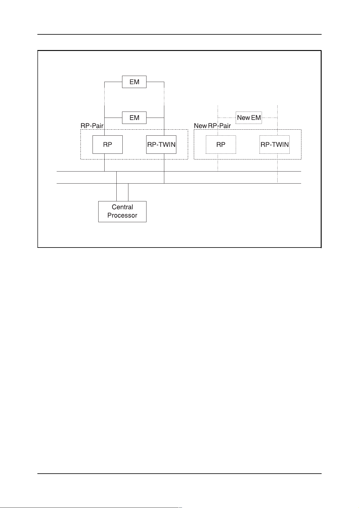
some cases be used for the extension. Figure 2.2, on the next page, shows
the parts of the system that are handled in this chapter.

03802-EN/LZM 112 18 R1 3

Exchange Data Basic

Figure 2.2

The control part of the AXE system

First of all, the hardware of the RP pair must be connected and the power
must be connected to the magazine. Howe ver , this i s not enough as the RP
pair must be defined in data as well. This means that some initial data is
loaded into the system and that the parts that take care of the maintenance
of the RPs are informed of their location. The location of the RP pair is
marked by an address strap on one of the boards in the RP and that address
must always be used when using commands related to the RP. The Opera­tional Instruction “Connection of RP” describes the actions required for
the definition. The first command used for the definition of an RP pair is
the EXRPI command.

EXRPI:RP=rp,RPT=rpt,TYPE=type;

The RP and RPT parameters are used to indicate to the system the
addresses allocated to the RPs with the address strap. The TYPE parameter
is used to indicate the version of the RP as both old and new RPs can be
used in the same exchange. The Command Description of the command
EXRPI contains a list of valid RP types.

When the RP pair has been defined, the next step will be to define which
software units (programs) that should be loaded into the RP pair when
deblocked. The programs loaded into the RP should be some operating

4 03802-EN/LZM 112 18 R1

Device and Route Data

software and the regional software of the blocks connected to the RP (e.g.
the regional software of block BT1 is referred to as BT1R).

The command used to define the RP programs to be loaded is EXRUI.
This command will build up a table inside the APZ related to each RP pair.
The table can be used by the APZ when reloading it, e.g. in connection
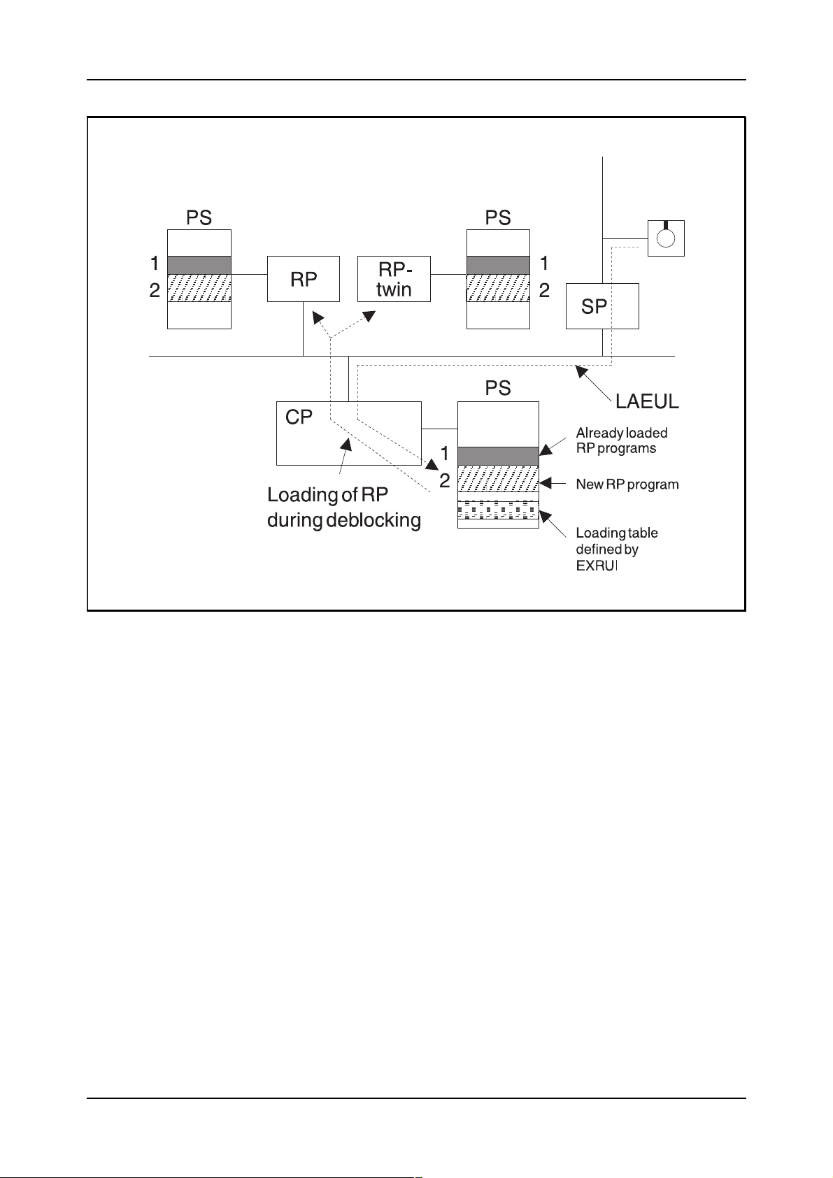
with deblocking. Then the software indicated in the table is sent to the Pro­gram Store of the RPs in the RP pair. This also means that a copy of all
regional software units must be a v ailable in the CP as a backup. When ne w
equipment is installed in the exchange (e.g. a new type of BT devices), the
new RP program must be loaded into the CP by means of command
LAEUL.

The parameters included in the EXRUI command are RP and SUNAME
or SUID. The RP parameter is used to indicate one of the RPs in the RP
pair (only one has to be specified). The SUNAME and SUID parameters
are used to indicate the name or the identity of the software units that
should be included in the RP pair . Which parameter to use is determined as
follows:

SUNAME This parameter is used if there is only one version of the

software unit loaded in the CP. An example of a software
unit name is BT1R.

SUID If there is more than one version of the RP program

loaded into the CP, this parameter must be used to indicate
which version to use. This parameter is used if the version
of a Regional Software unit is changed because of soft­ware update or function change. An example of the
parameter is “5/CAA1052105/1R2A02”. The correct
identities can be printed by using command LAEUP.

When the loading table has been defined, perhaps using several EXRUI
commands, the RP pair can be put into service by deblocking it. The
deblocking is done by using command BLRPE which first includes a test
of the RP and then a reload of the software units specified in the table.
Please study figure 2.3, on the next page.

03802-EN/LZM 112 18 R1 5

Exchange Data Basic

Figure 2.3

The new RP programs are loaded into the CP and defined for the RP pair

6 03802-EN/LZM 112 18 R1

When the data has been specified, the EXRPP command can be used to
check it. Please study figure 2.4.

Figure 2.4

Answer printout of command EXRPP

All the data related to an RP pair can be removed by the EXRPE com­mand. This command is used if the RP pair is to be removed from the
exchange.

Device and Route Data

2.1.3 Definition of Extension Modules

When the new RPs have been defined, it is time to define the equipment
they should control. As you probably know, this equipment is located in
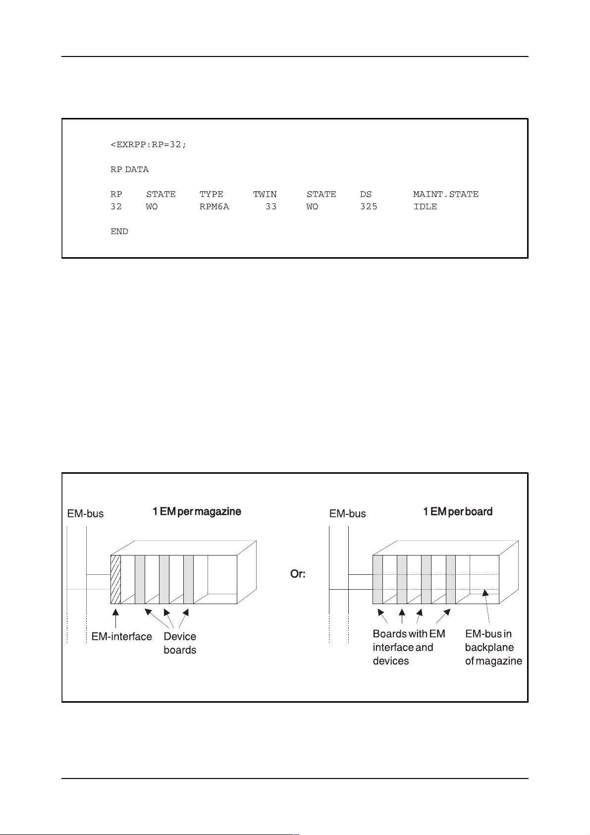
Extension Modules using the same type of interface to the RPs. Figure 2.5
shows the principle of connecting two different types of EMs to the EM
bus.

Figure 2.5

Connection of two different types of EMs to the RP pair

03802-EN/LZM 112 18 R1 7

Exchange Data Basic

When the EMs are defined, the data in both the APZ and the blocks that
own the hardware is updated with various types of information. The data
in the block that controls the hardware is updated with information about
the address of the hardware (RP and EM addresses). This information is
required when sending signals to the hardware for initiating functions in
the hardware.

The command used to define the EMs is EXEMI and the following param­eters are included for a normal definition:

EXEMI:RP=rp,RPT=rpt,EM=em,EQM=eqm;

RP: Indicates the RP that controls the EM in normal cases.
RPT: Indicates the stand-by RP. This RP must be the twin RP in an

RP pair.
EM: Address of EM (an address strap is used).
EQM: Used to indicate the equipment type and identity of the devices

in the EM. Example: EQM=BT1-32&&-63.
When the EM has been defined, it can be deblocked by command

BLEME. This means that the EM is put into service from a control point
of view. The devices in the EM are probably still blocked as more data
related to the devices must be specified.

If an EM is to be removed from the exchange, command EXEME is used.
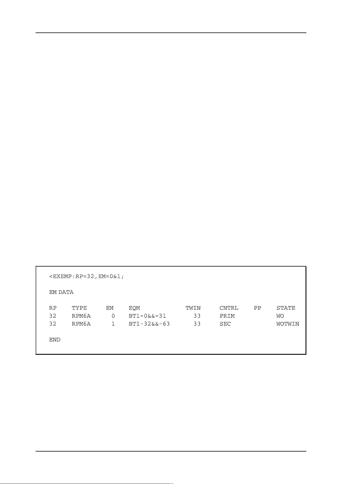
When the data has been specified, the print command EXEMP can be
used. Figure 2.6 shows an example of a printout of command EXEMP.

Figure 2.6

Answer printout of command EXEMP

2.1.4 Definition of Routes

Before we discuss how routes are connected and defined in the software of
AXE, the route concept in AXE should be studied. In AXE, the concept
“route” has been extended slightly if compared with other, analog systems.

8 03802-EN/LZM 112 18 R1

Device and Route Data

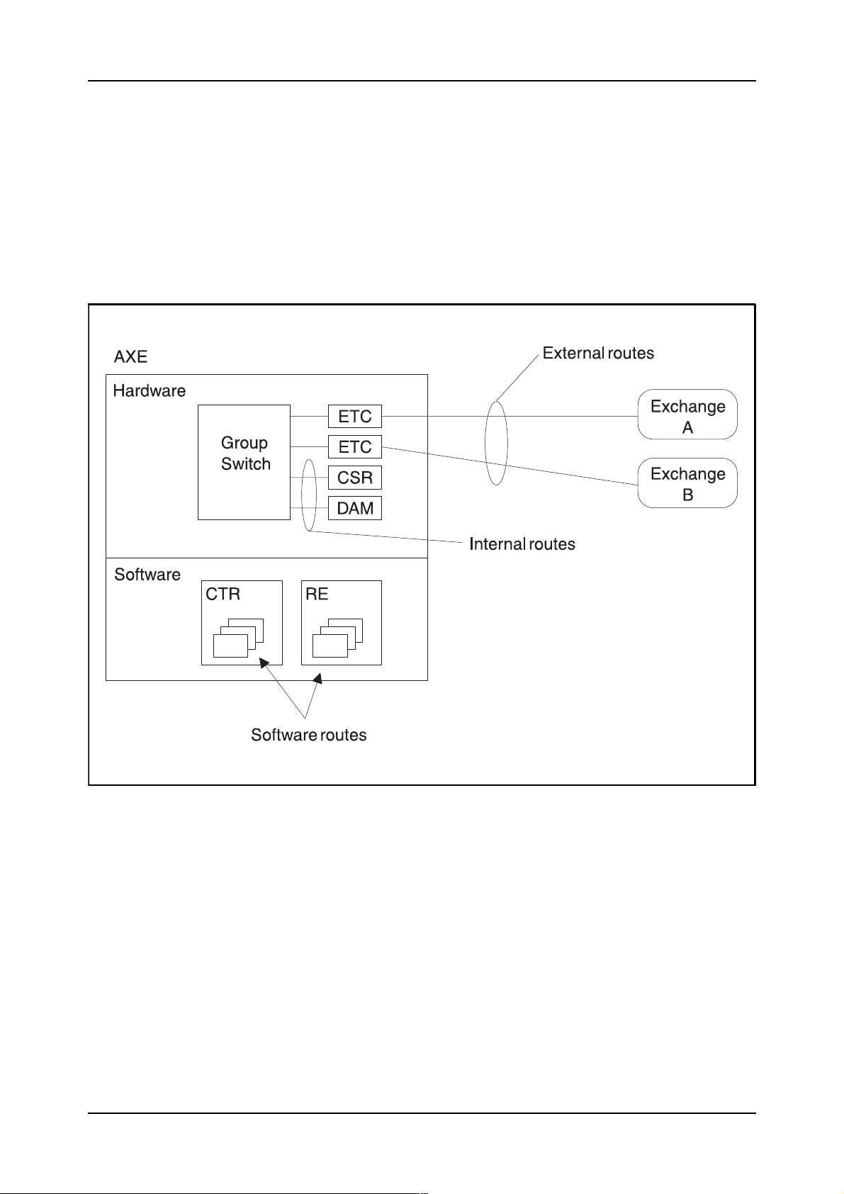
There are basically three types of routes in the system:

1. External routes, e.g. routes to other exchanges

2. Internal routes, e.g. routes to Code Senders and Announcing

Machines

3. Software routes, e.g. routes to subscriber services or routes for regis-

ter individuals.

Figure 2.7 shows the three variants of the routes.

Figure 2.7

The three types of routes used in AXE

03802-EN/LZM 112 18 R1 9

Exchange Data Basic

All the three types of routes require “Route Data” in order to function in a
specified way. Route data is, as the name says, data related to a route in the
exchange. Examples of route data for an external route is the type of sig­nalling system used, the function of the route (incoming or outgoing) and
the number of devices connected to the route. The route data is stored in
the block to which the hardware belongs. The Operational Instruction
“Connection of route for BT” is one of the documents available that
describes the commands that should be used. In this chapter, only the com­mands and the most common parameters are described. Supervision and
connection of the devices to the Group Switch are handled in other parts of
this Module.

How, then, is the route data defined in the exchange? The answer is the
two commands
lowing meaning:

•

EXROI
This command is used to initiate the route for the very first time. The
parameters included in the command are (not all shown):

−

EXROI

R, Route name
This parameter gives the route a name consisting of up to 7
characters. Characters like #, % and + can be used in the route
name to distinguish between incoming and outgoing routes.

and

EXRBC

. The two commands have the fol-

−

DETY, Device type
The device type indicates the type of de vices used in the block.
The parameter should be the same as the block name of the
block used for the route (e.g. BT1).

−

FNC, Function Code
The function code is used to indicate the function of the route.
The meaning of the parameter must be fetched from the Appli­cation Information of the block indicated in DETY. For exter­nal routes, the parameter is usually used to indicate the traffic
direction of the route.

•

EXRBC
This command is used when more route data is to be assigned to the
route. Also existing routes can be changed by this command. The com­mand has several parameters of which only a few are explained here:

−

R1, Register Signalling Route
This parameter is used to indicate if another route must be
used for the register signalling. If MFC (Multi-Frequency
Compelled) signalling is used, the route name of the Code
Sender route is indicated here. Figure 2.8 shows the principle.

10 03802-EN/LZM 112 18 R1

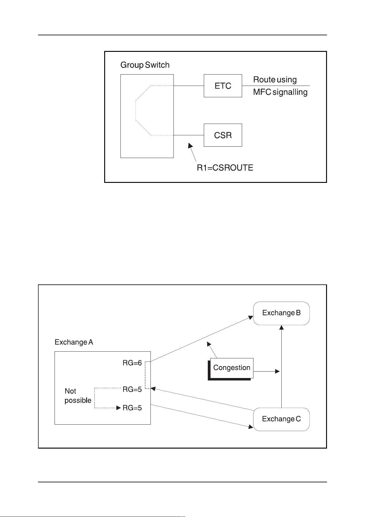
Figure 2.8

Register signalling route

Device and Route Data

−

RG, Route Group
The Route Group parameter is used to prevent the traffic from
one exchange to be returned to the same exchange (also
referred to as “return blocking”). By giving all routes to and
from the same exchange the same RG value, the system will
not route the traffic back to the same destination.
Please study figure 2.9.

Figure 2.9

Return blocking principle

03802-EN/LZM 112 18 R1 11

Exchange Data Basic

−

RO, Origin for route analysis
For incoming routes, this parameter can be used if the Route
Analysis should be made differently for this route compared
with others. More about this in the Unit describing Route
Analysis.

−

PRI, Priority
Some incoming routes can be given priority. This parameter
can be used in various analyses in the exchange.

−

MB, Modification of B-number
This parameter can be used to add or delete digits from the B­number.

As already mentioned, there are several other parameters included in the
EXRBC command. For more details please study the Command Descrip­tion and the Application Information for the blocks concerned.

When all the route data has been specified for the route, and if the route
should be put into service, it should be deblocked by using the BLORE
command. Note that only outgoing routes can be blocked/deblocked. The
command BLORP can be used to check if any outgoing route is blocked in
the exchange.

2.1.5 Connection of Devices to the Route

When all the route data has been specified, it is time to connect devices to
the route. Howev er, before this is done, the devices should be connected to
the Group Switch. How that is done is described in Unit 3 of this Module.

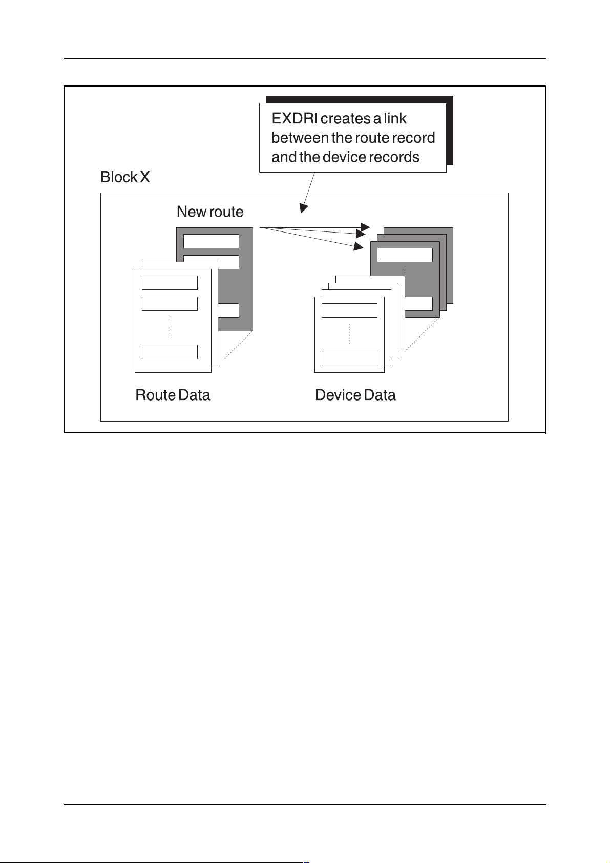
Before this step is started, the route has been properly defined by means of
EXROI and EXRBC. However, no devices are connected to the route. The
EXDRI command is used to make a connection in data between the
devices and the route:

EXDRI:DEV=dev,R=r;

In case of ISDN services special devices are required, but this is not the
case for ordinary telephone calls.

Figure 2.10 shows what the command does in the data of the block.

12 03802-EN/LZM 112 18 R1

Device and Route Data

Figure 2.10

The effect of command EXDRI in the data of a block

When all the devices have been connected to the route, they should be
taken into service by using the command EXDAI. This command will
change the state of the devices from “Pre-post service” to “service”.

Finally, the devices can be deblocked by using command BLODE. That
will enable the system to use the devices in traffic handling.

In most cases, the supervisory functions should be connected to the route
in order to activate functions like “Blocking supervision”. In case of an
extension of an existing route, the data related to t he supervisory functions
should be changed (the number of devices included in the route has
changed).

03802-EN/LZM 112 18 R1 13

Exchange Data Basic

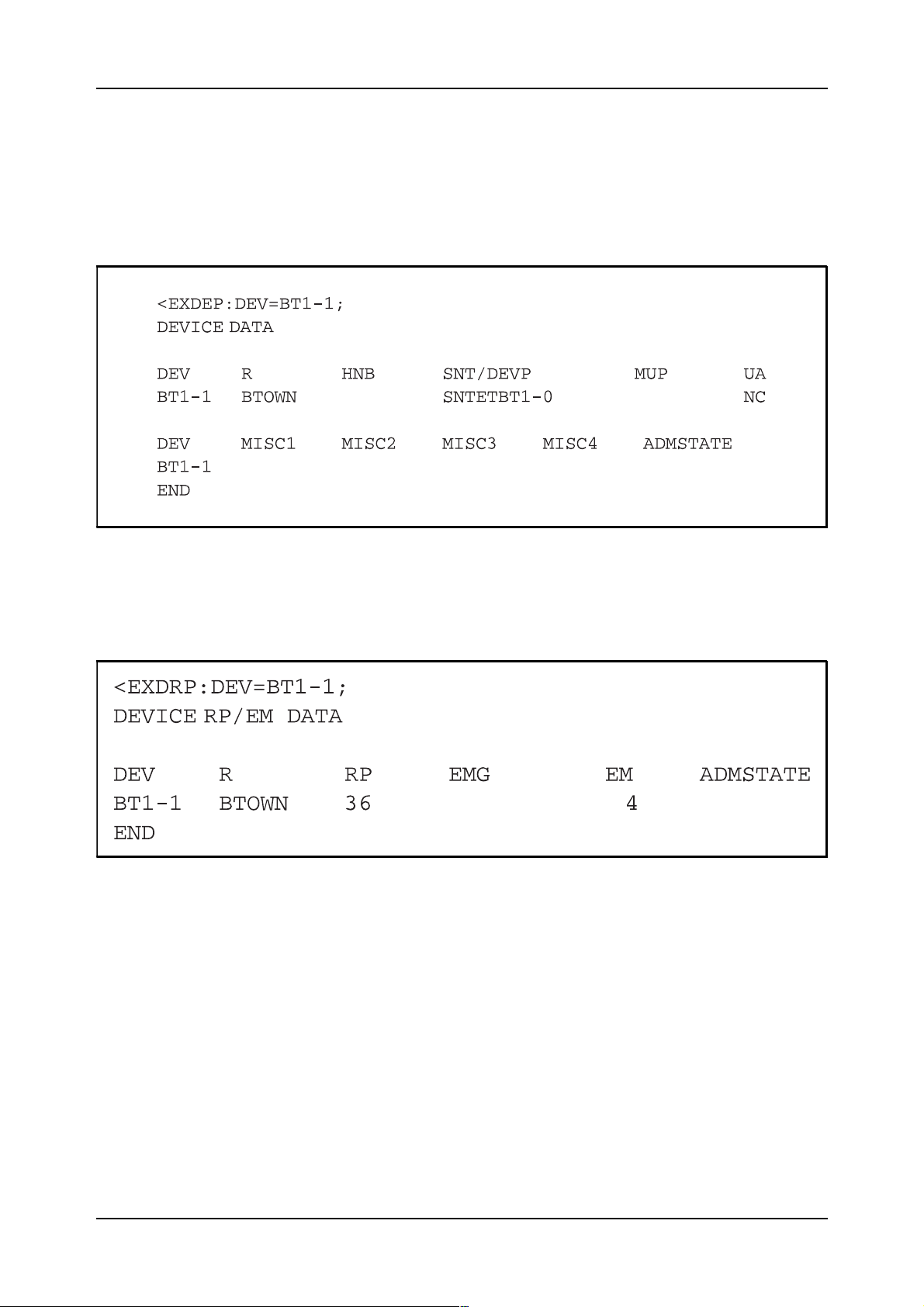
2.1.6 Printout of Device and Route Data

When the data has been defined, and also during the definition, the data
loaded can be printed by using print commands. Some of the most useful
commands are shown below.

EXDEP, please study figure 2.11.

Figure 2.11

Printout of device data

EXDRP, please study figure 2.12.

Figure 2.12

Printout of the RP and EM that the device belongs to

14 03802-EN/LZM 112 18 R1

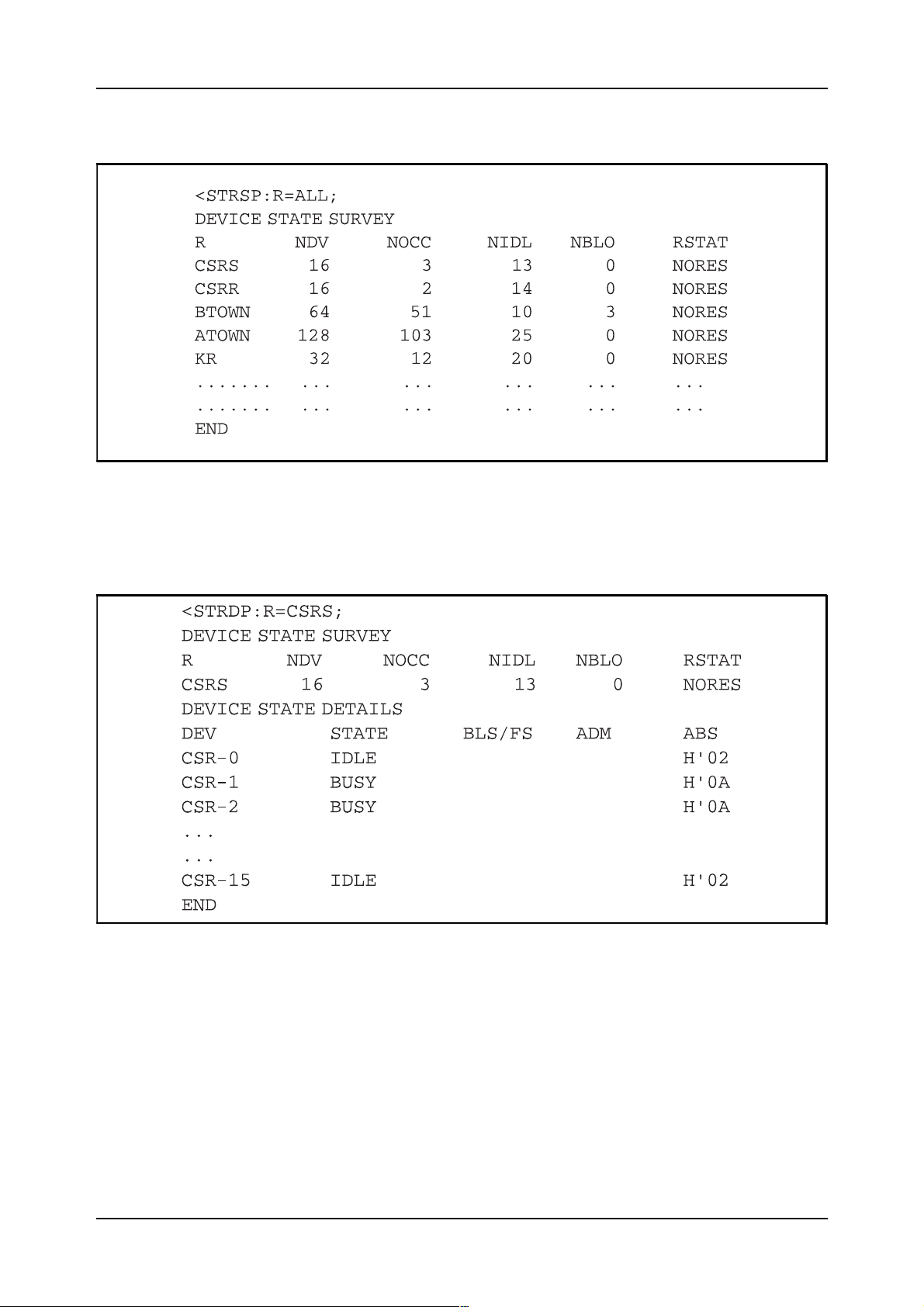
STRSP, please study figure 2.13.

Figure 2.13

Printout of device state survey

Device and Route Data

STRDP, please study figure 2.14.

Figure 2.14

Printout of device state survey and details

03802-EN/LZM 112 18 R1 15

Exchange Data Basic

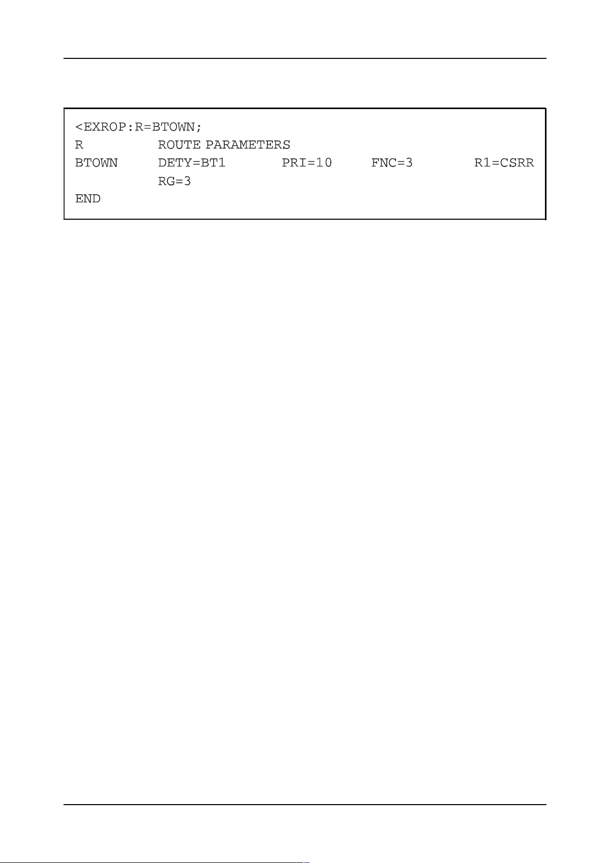
Figure 2.15

Printout of route data

EXROP, please study figure 2.15.

16 03802-EN/LZM 112 18 R1

2.2 Supervision Data for Trunks

2.2.1 General Principles of Supervision

Telephony devices interwork with their environment, such as subscribers,
other exchanges and transmission equipment. A single disturbance in one
device does not mean that the device is faulty. The disturbance might come
from the environment. For that reason, the supervision of telephony
devices is rather a slow process. Several calls causing disturbances will in
many cases have to be registered before any actions are taken by the sys­tem. In some cases, the supervisory period will cover several days.

The actual supervision of the devices is performed by the blocks that own
the hardware. As an example, disturbances in devices belonging to block
BT1 are also registered in that block. Disturbances are registered by means
of counters in the software. In some cases, the counters are common to one
route and in others, there is one disturbance counter per device.

The errors that are to step the disturbance counter are to a great extent
determined by the protocol of the signalling system. Any abnormal event
such as time out, signalling errors and state error, are registered in the dis­turbance counter.

Device and Route Data

When should an alarm be initiated and what alarm class should be used? Is
the supervision activated or not? These types of questions are usually han­dled by blocks specially dedicated to the administration of the supervisory
functions. These blocks are located in the OMS, Operation and Mainte­nance Subsystem, and they handle functions such as:

•

changing of alarm levels

•

changing of alarm classes

•

activation and deactivation of the supervision

•

handling of commands and printouts.

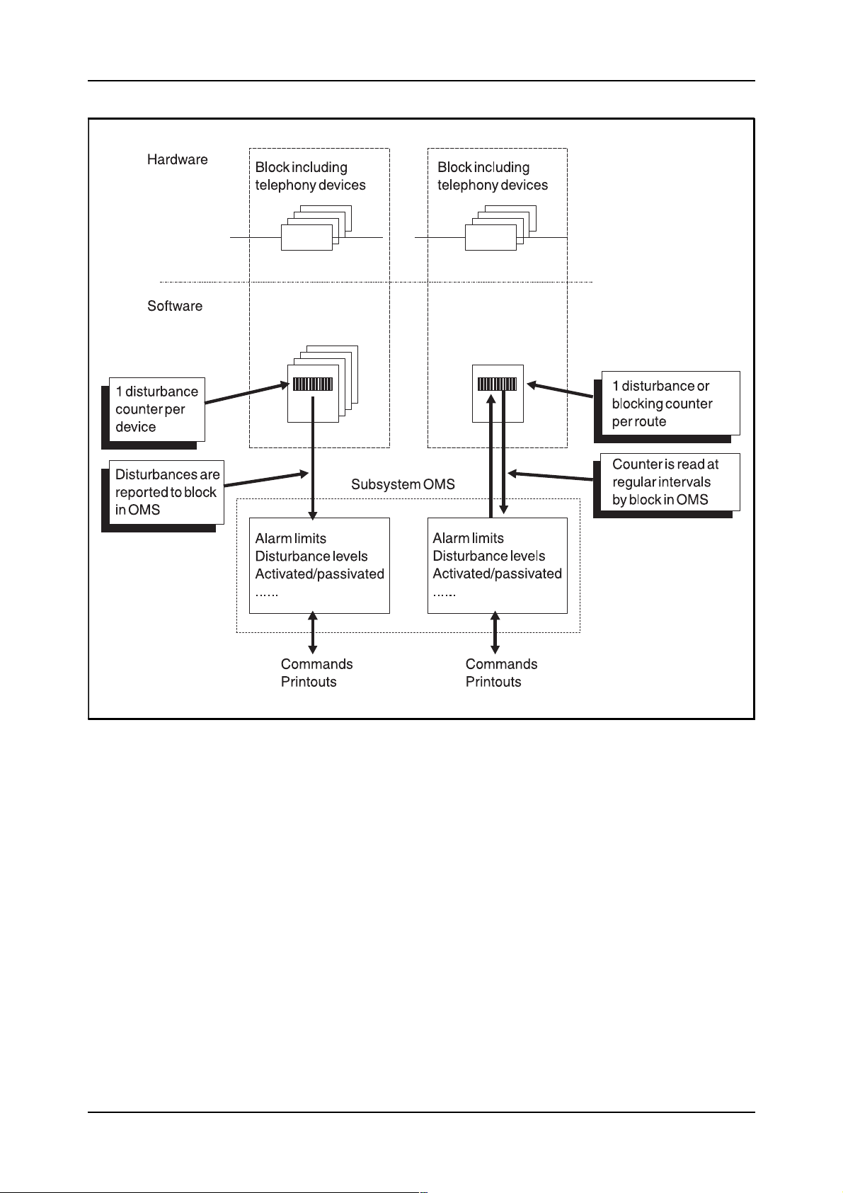
When the supervision is activated, the block in OMS that administers the
function, reads the disturbance counters at regular intervals. The time
between the readings is usually between 10 seconds and 1 minute. If the
readings are too frequent, they will load the processor unnecessarily. The
read disturbance counters will then be compared with the stated alarm lev­els which are stored inside the block. For some types of functions, the
block that own the disturbed device will report each disturbance to the
block that handles the administration related to the function. Figure 2.16,
on next the page, shows an example of how the supervision can be made.

03802-EN/LZM 112 18 R1 17

Exchange Data Basic

Figure 2.16

General principle of supervision of telephony devices

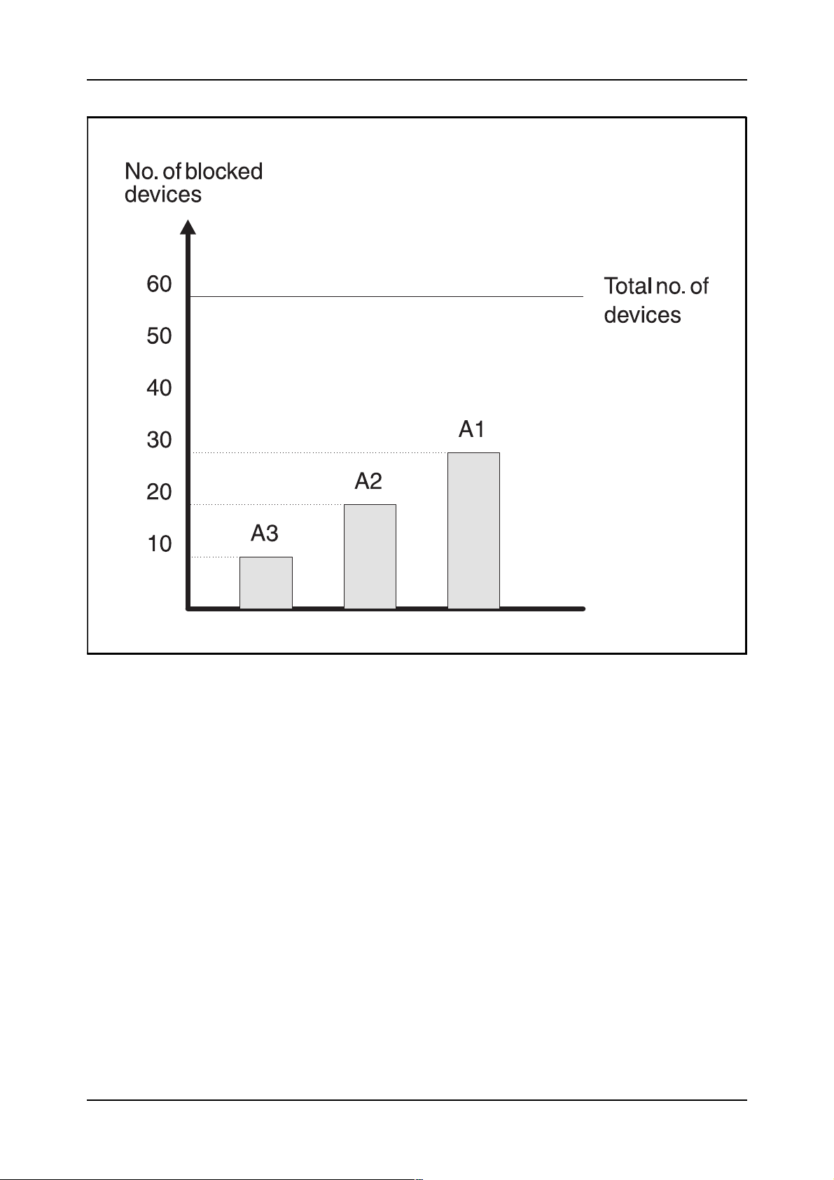
2.2.2 Blocking Supervision

This function, handled by block BLOS, checks that the number of blocked
devices in a route does not exceed a preset value. The function counts the
number of manually, automatically and control blocked devices. If
required, the function can use several alarm limits tied to different alarm
classes. Figure 2.17 shows the principle.

18 03802-EN/LZM 112 18 R1

Device and Route Data

Figure 2.17

Alarm limits in the blocking supervision, example

The Blocking Supervision is always initiated per route and all commands
and printouts are related to a given route in the exchange. The function can
be used to supervise routes belonging to blocks of type BT, AS, CR, CS
and KR.

If no data has been specified for a route, e.g. the route has just been initi­ated, new supervision data will hav e to be loaded b y means of the BLURC
command. The parameters in the command are:

R=r,LVB=lvb1[&lvb2][&lvb3],ACL=acl;

The “R” parameter indicates the name of the route (the same as in
EXROI). The “LVB” parameter, Limit Value for Blocking, is used to indi­cate the maximum number of blocked devices in the route. If several val­ues are to be used (as in figure 2.17) the values are listed and separated by
“&”. The last parameter is “ACL”, Alarm Class, which is used to indicate
the alarm class the alarm should have if the limits are exceeded. If several
limits have been specified, this parameter indicates the alarm class tied to
the first limit value. An example is:

03802-EN/LZM 112 18 R1 19

Exchange Data Basic

BLURC:R=ALPHA,LVB=10&20&30,ACL=A3;

If this command is used, the system will initiate the following alarms:
A3 alarm: if the number of blocked devices is between 10 and 20.
A2 alarm: if the number of blocked devices is between 20 and 30.
A1 alarm: if the number of blocked devices exceeds 30.
The blocking supervision of a route can be temporarily disconnected dur-

ing maintenance activities or other changes related to the route. It is also
possible to disconnect the blocking supervision permanently. The com­mands used to disconnect and reconnect the blocking supervision are:

BLURE:R=r[,PERM];
BLURI:R=r;

BLURE

The

PERM

“

command is used to disconnect the supervision. If the

” parameter is used, the supervision is permanently disconnected.
This means that the supervision data is erased. When the supervision is to
be connected again, the

BLURI

command is to be used.

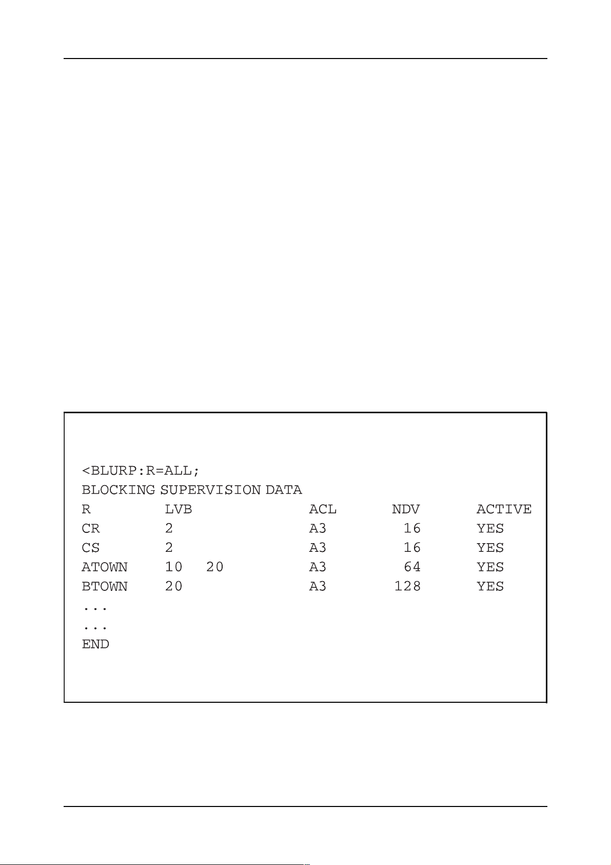
The supervision data can be printed by using command

BLURP

example of the printout generated can be seen in figure 2.18.

. An

Figure 2.18

An example of a printout of the blocking supervision data

20 03802-EN/LZM 112 18 R1

2.2.3 Disturbance Supervision of Devices

This function supervises that the proportion of the number of disturbances
to the number of selections will not exceed a preset v alue. The supervision
is used to supervise individual devices of type CS, CR and some variants
of BT (not all types of BT can have this type of disturbance supervision).
In case of analogue CS and CR devices, they are blocked if a number of
consecutive disturbances are detected.

Disturbances are defined as disconnections not caused by the subscriber or
not allowed traffic cases. Examples are time out, not valid signals and
abnormal states in the signalling.

When a new route is defined which should have this type of supervision,
the data must be loaded by means of command DUIAC. The parameters
included in the command are:

DUIAC:R=r,ADL=adl,ACL=acl;

Parameter “R” indicates the name of the route concerned. Parameter
“ADL”, Allowed Disturbance Level, indicates the level in percent. If this
level is reached, an alarm with the alarm class according to parameter
“ACL” will be generated. The possible values in ADL are 1, 2, 4, 5, 10,
20, 25, 33 and 50%.

Device and Route Data

How, then, is the supervision made in block DISSD which handles the
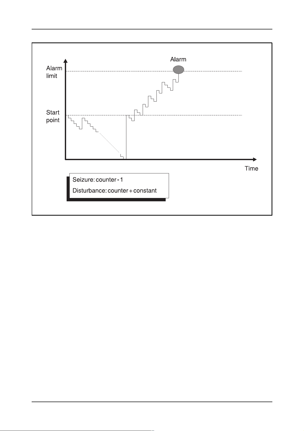
function? The answer is a disturbance counter used to record both the sei­zures and the disturbances. Figure 2.19, on the next page, shows the prin­ciple.

03802-EN/LZM 112 18 R1 21

Exchange Data Basic

Figure 2.19

The use of a disturbance counter

For each seizure of the device, the counter is decremented by one. In case
of a disturbance, the counter is incremented by a value dependent on the
parameter ADL, Allowed Disturbance Level.

The loaded data can be printed by using the print command DUISP. Figure

2.20 shows an example of such a printout.

22 03802-EN/LZM 112 18 R1

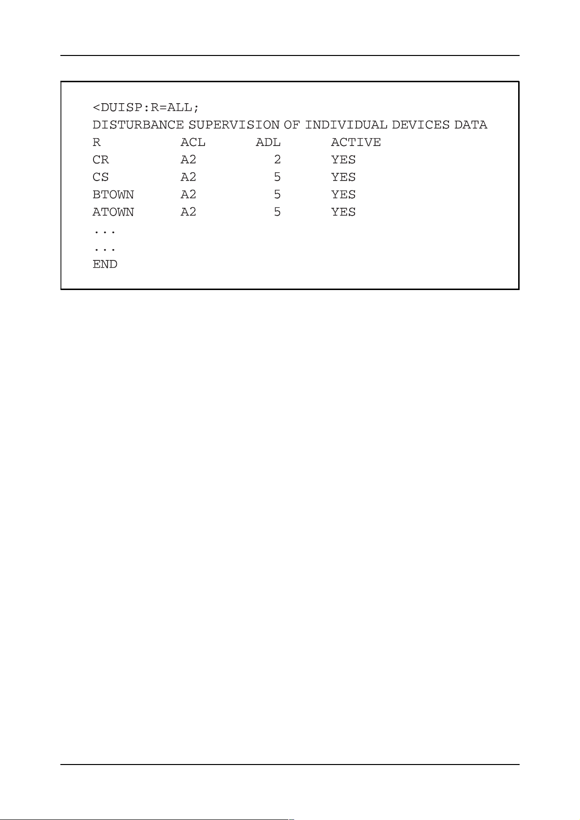
Figure 2.20

The printout of the Disturbance Supervision of Individual Devices, example

Device and Route Data

2.2.4 Disturbance Supervision of Routes

This function is very similar to the one described in the previous chapter.
The only major difference is that this function supervises the disturbance
level of each route, not individual devices. The function is implemented in
block DISSR and the routes that can be supervised are the ones of type BT .
The function uses a disturbance counter like the one described in figure

2.19, with the only difference that there is one counter per route.
When a new route has been introduced in the exchange, or if some e xisting

data should be changed, command DUDAC shall be used. The parameters
included in the command are:

DUDAC:R=r,ADL=adl,ACL=acl;

Parameter “R” is used to indicate the route. Parameter “ADL”, Allowed
Disturbance Level, specifies the maximum disturbance level allowed in
the route (in percent). If this value is exceeded, an alarm with the alarm
class according to parameter “ACL” will be generated. The possible dis­turbance levels in parameter ADL are 1, 2, 4, 5, 10, 20, 25, 33 and 50%.

03802-EN/LZM 112 18 R1 23

Exchange Data Basic

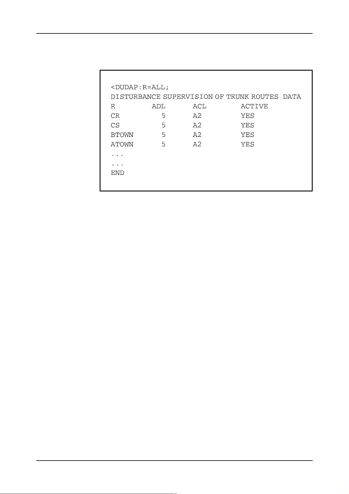
When the data has been loaded, it can be printed by using the print com­mand DUDAP. Figure 2.21 shows an example of such a printout.

Figure 2.21

Printout using command DUDAP

2.2.5 Seizure Quality Supervision of Devices

This function is used to supervise the ratio (quotient) of the number of sei­zures to the number of normal calls. What, then, is meant by “normal
call”? This is nothing but a time (usually set to 60 seconds) specified by
command which is used to indicate a minimum duration of a normal call.
This function utilizes the fact that subscribers connected to bad lines,
replace earlier than if they were connected to normal lines.

The average quotient is also calculated for the devices in the same route,
and each device in the route is compared with this value. If any of the
devices deviates more than a command specified value, an alarm will be
initiated. Two limits are used by the function:

•

one limit which indicates that the device is suspected of being faulty

•

one level which indicates that the device should be blocked.

When the function is started the very first time, i.e. when the exchange is
installed, the time for a “normal call” is loaded. This is done by using the
command SEQAC . This command ca n al so be used when time is cha nged
if other conversation times are used in the exchange (can be detected by
means of Traffic Recording). An example of how the time is changed is:

SEQAC:CTIME=55;

The normal conversation time is, in this case, set to 55 seconds. The time
can vary between 10 and 255 seconds.

24 03802-EN/LZM 112 18 R1

Device and Route Data

If the supervision is to be initiated for a new defined route in the exchange,
the same command is also used to load the supervision data related to the
function. An example of the command is:

SEQAC:R=BTOWN+,ACL=A3,QUOS=30,QUOB=60;

If this command is used, the supervision will be initiated for the route
“BTOWN+”. If any abnormal devices are detected, an A3 alarm will be
generated. If a device deviates by more than 30% from the average quo­tient, the device is suspecte d of being faulty. In that case, the device is still
in traffic (only fault marked). If a device deviates by more than 60% from
the average quotient, it will be blocked.

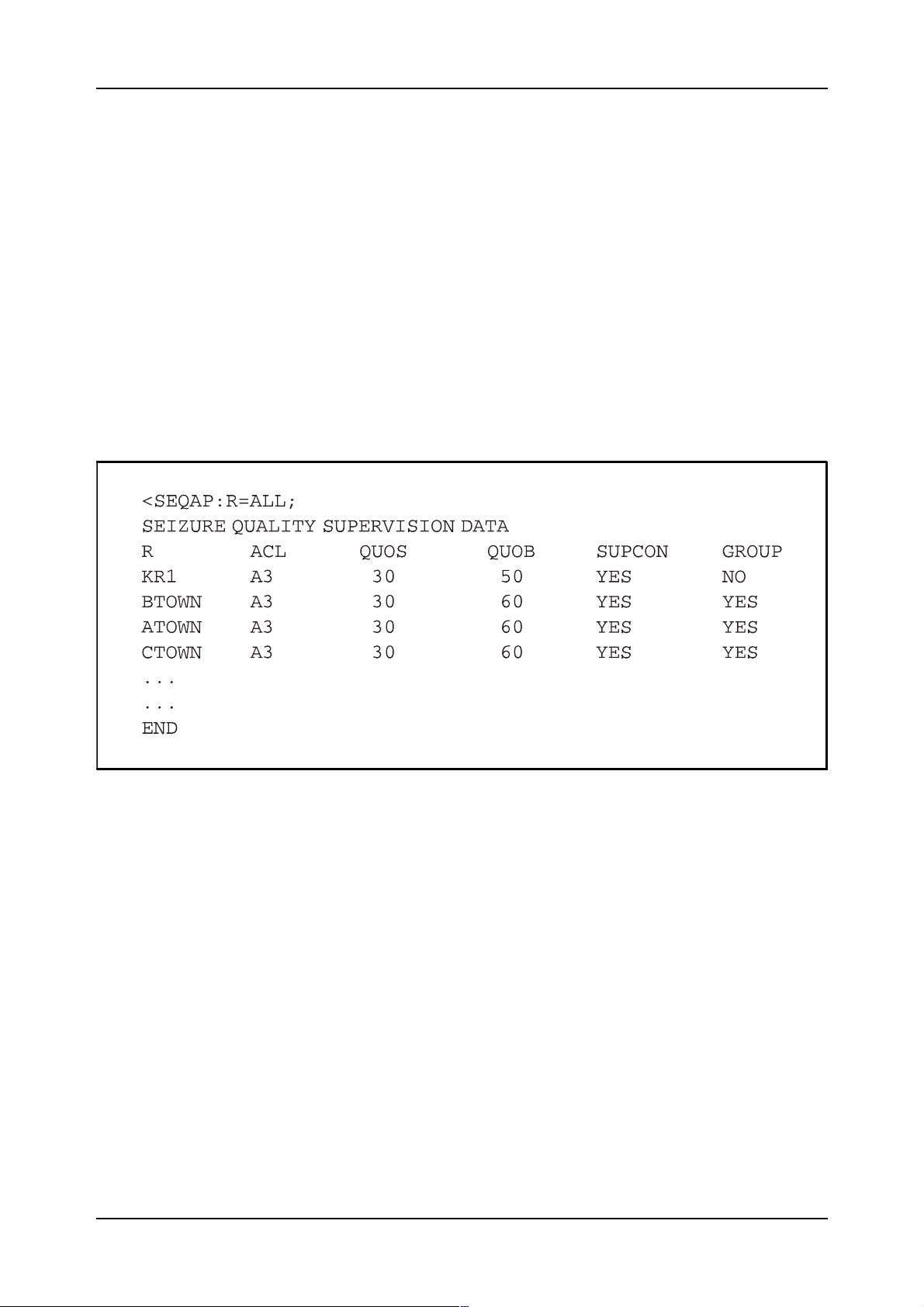
The data specified for a route can be printed by using command SEQAP.
Figure 2.22 shows an example of a printout generated by command
SEQAP.

Figure 2.22

Example of printout related to Seizure Quality Supervision

2.2.6 Groups for Seizure Quality Supervision

The Seizure Quality Supervision function uses the routes as groups if
nothing is indicated to the system. If there are requirements that new
groups should be defined, command SEQGI can be used to group routes
together. This means that the average quotient (Q) will be calculated for
the whole group. Different types of routes with different characteristics
can be grouped together with this function. Command SEQGI has only
one parameter:

SEQGI:R=r....;

Several routes can be specified in one command and the number of routes
included in one group is unlimited. When the groups have been specified,
command SEQGP can be used to print the routes included in each group.
Please study figure 2.23.

03802-EN/LZM 112 18 R1 25

Exchange Data Basic

Figure 2.23

A printout of route groups

If changes should be made in any route group, the command SEQGC will
be used. The command can either remove one or several routes from a
route group, or it can be used to split a route group. The parameters
included in the command are:

SEQGC:R=r...[,ALL];

If only the “R” parameter is used, the specified route(s) will be removed
from the route group. If the “ALL” parameter is included as well, the
whole route group will be split up.

2.2.7 Seizure Supervision of Trunks

Most of the supervisory functions studied so far, uses live traffic for their
supervision. In order to detect errors for lines not having any traffic at all,
or for lines which are continuously busy, the Seizure Supervision function
is used (implemented in block SETS).

The principle of the function is to check that all lines in a route have been
selected at least once during a specified period. A seizure is registered
when a B-answer is received. If no seizures are registered during the
period, an alarm will be generated.

The command used to load and change the data related to the function is:

SETAC:PL=pl,ACL=acl;

Parameter “PL”, Period Length” is used to specify a period stated in days.
If a route with unused lines is detected at the end of the period, an alarm
with the alarm class as specified in parameter “ACL” will be generated.
The period length can vary between 1 and 3 days.

26 03802-EN/LZM 112 18 R1

Device and Route Data

When the data has been specified, it can be printed by means of command
SETAP. Please study figure 2.24.

Figure 2.24

An example of data generated by command SETAP

03802-EN/LZM 112 18 R1 27

Exchange Data Basic

2.3 Chapter Summary

• Regional Processors

•

An RP pair can maximum control 16

•

An EM is a magazine which contains a number of devices of the same
type.

route

•

A

•

A route can be going between exchanges or internal or be a software
route.

•

An AXE 10 exchange has built in supervision.

is a group of devices having the same characteristics.

• Blocking Supervision

route.

• Disturbance Supervision

on routes.

• Seizure Supervision

never seized or permanently seized in a preset supervision period.

• Seizure Quality Supervision

tion.

(RPs) always work in a pair.

Extension Modules

monitors the number of blocked devices on a

monitors line and register signalling quality

monitors routes to detect devices which are either

monitors the number of calls of short dura-

(EMs).

28 03802-EN/LZM 112 18 R1

3. Connection to Group Switch

Chapter Objectives

After completing this chapter the participant will be able to:

• Understand the main principles of the Group Switch.

• Describe the basic blocks in subsystem GSS.

• Describe the basic hardware of the Group Switch.

• Perform connection of SNT and devices to the GSS.

• Perform connection of DIP.

Figure 3.1

Chapter Objectives

3.1 GSS in General

The Group Switching Subsystem, GSS, belongs to the APT and contains
both hardware and software. As its main task GSS connects an incoming
channel to an outgoing channel.

As GSS is designed to work with different transmission media and sys­tems, it is possible to hav e PCM links as well as analog links . This enables
GSS to connect digital lines from Remote Subscriber Stages, RSS, or other
switches. This is done via an ETC (Exchange Terminal Circuit) for digital
links, or via PCD (Pulse Code Device) for analog links. More about ETC
and PCD later on in this chapter.

Generally speaking, we can say that GSS connects one inlet in the Group
Switch to one outlet, since all telephony devices connected to an AXE 10
exchange need to be through connected via GSS. The Group Switch has
one inlet and one outlet per device/channel. This makes it possible to have
a bothway connection.

3.1.1 Basic Functions, Hardware and Software.

The Group Switching Subsystem has the following functions:

a) Selection, connection and disconnection of speech or signal

paths through the Group Switch.

b) Supervision of hardware in the subsystem by continuous par-

ity checks.

c) Supervision of digital links connected to the switch.

03802-EN/LZM 112 18 R1 29

Exchange Data Basic

d) Maintaining a stable clock frequency or synchronization of the

clock frequency of the network.

To make these functions possible in GSS, lots of functions have been
implemented in different function blocks. Some of these which are related
to traffic handling are described in this chapter. Figure 3.2 shows the most
important blocks.

Figure 3.2

The basic blocks in GSS related to traffic handling and synchronization

30 03802-EN/LZM 112 18 R1

Connection to Group Switch

A brief description of the different blocks follows below:

GS, Group Switch

1.

It is implemented in central software only and it is responsible for
storing connection information and also interfaces towards some
other subsystems.
Also, it should be mentioned that the former version of the GS func­tion block contained hardware and some other functions that now are
implemented in other function blocks. Note that this earlier version
is still available in some application systems.

GSM1/GSM2, Group Switch Maintenance

2.

These two blocks assist block TSM with maintenance functions
regarding TSMs and SPMs. They contain administration functions
for all SNTs (Switching Network Terminals) connected to the
switch.

TSM, Time Switch Module

3.

This block consists of hardware, central and regional software. Its
hardware is the TSMs and SPMs. It handles the normal switching
functions such as connection and release of speech paths, adminis­tration of TSMs and SPMs as well as counters for statistics and traf­fic measurements. This function block did not exist in the former
version of the GSS.

GSBOARD, Group Switch Board Names

4.

This block is fully realized in central software and some of its main
functions are translation of fault cases into suspected printed boards
for printing when fault diagnostic functions are performed. This
block did not exist either in the previous version of the GSS.

CLT, Clock Pulse Generation and Timing

5.

The hardware of this block is the three Clock Modules which supply
the TSMs and the SPMs with clock pulses. It also handles mainte­nance functions as well as counters for statistics and traffic measure­ments. Due to the introduction of new clock modules the CLT
function block has been revised.

NS, Network Synchronization

6.

The digital exchanges must be synchronized with each other. Block
NS contains functions, implemented in both hardware and software,
for synchronization of the network.

Blocks for Operation and Maintenance

7.

There are several blocks related to the O&M of the GSS. These
blocks supervise the hardware, handle commands, alarms, handle
temporary errors in the hardware and perform routine tests of the
hardware.

Subsystem GSS is a central part of the system as almost all calls and sig­nalling systems use the switch to connect hardware to various channels.

03802-EN/LZM 112 18 R1 31

Exchange Data Basic

Examples of other subsystems that interwork with GSS are:

For traffic handling:

TCS for connection of A and B-subscribers
TSS for connection of Code Senders / Code Receivers and trunk

lines

SSS for call release and connection of subscribers and PABX,

(Private Automatic Branch Exchange)
BGS for call set-up within the Business Group
ESS for operator calls, monitoring and subscriber services. Function

blocks CCD (Call Conference Device) and MJD (Multi Junctor

Digital) belonged to the GSS earlier but have been incorporated

in ESS.

For Operation and Maintenance:

OMS handling of test calls (call set-up and release).

Statistics:

STS Statistics & Traffic Measurement Subsystem.

Others:

OPS for trunk offering and operator-assisted calls
SUS subscriber services requiring three-party conference calls and

other services requiring conference calls (Call Waiting)
MTS for connection of Code Senders and other equipment included

in subsystem MTS.

32 03802-EN/LZM 112 18 R1

Connection to Group Switch

Figure 3.3 gives some examples of subsystems interworking with GSS.

Figure 3.3

Other subsystems that interwork with GSS, example

03802-EN/LZM 112 18 R1 33

Exchange Data Basic

3.1.2 Hardware Structure and Switching

In order to ensure adequate flexibility, the Group Switch has been
designed and structured into modules referred to as Time Switch Modules
(TSM) and Space Modules (SPM). The number of TSMs and SPMs
required in an exchange depends on the number of trunk and subscriber
lines.

To each Time Switch Module, up to 16 PCM systems can be connected.
This means that each TSM has 16x32=512 inlets, or Multiple Positions.
Each 32-channel PCM system is connected to the TSM in a so called
Switching Network Terminal Point, SNTP. See figure 3.4. The “Switching
Network Terminal, SNT” is a common term for all type of equipment that
can be connected to the Group Switch. SNT is, however, a software con­cept and represents the software connection of the physical hardware to
the Group Switch.

Examples of equipment that can be connected to the GS are:

•

Exchange Terminal Circuits, ETC

•

Conference Call Devices, CCD

•

Pulse Code Devices, PCD.

The PCD is used if analog devices should be connected to the GS. The
PCD is nothing but an analog-digital converter. Figure 3.4 shows the prin­ciple.

Figure 3.4

Connection of devices to the Time Switch Module

34 03802-EN/LZM 112 18 R1

Connection to Group Switch

1. The speech samples originating from the subscribers (or the signals

from signalling devices such as Code Senders) are stored in a speech
store referred to as Speech Store A, SSA. Each channel in the PCM
systems connected to the TSM has its own storage position in SSA.
This means that the SSA has 512 store positions, one for each chan­nel (16x32).

2. We can now introduce the concept of multiple position (MUP)

which is the common term used when talking about either channels
or storage positions within a TSM.

3. To make it possible to switch between TSMs, the Space Module

(SPM) is used. The SPM is also used for speech samples that are to
be sent back to the same TSM in the case when the A-party and B­party are connected to the same TSM. More about the SPM later on.

4. When the SPM has switched the speech sample and sent it to the

correct TSM, the sample is stored in another store. This store is
referred to as Speech Store B, SSB. As with SSA, each channel in
the connected PCM systems has its own store position. This means
that the relationship between channel and store position is fixed in
both SSA and SSB. Figure 3.5 shows the general principle.

Figure 3.5

The connection of the channel used by the A-subscriber

Within a Time Switch Module, no connection is provided between the
incoming and the outgoing channels (SSA and SSB). An incoming speech
sample is always sent via the Space Module before it is stored in SSB. In

03802-EN/LZM 112 18 R1 35

Exchange Data Basic

the GS, there is full availability. This means that any position connected to
the GS can be connected to any other position via an SPM (from one TSM
to another or within the same TSM). To make it possible to have a Group
Switch with a size varying from some thousand multiple positions to 65
thousand, 64K, the number of SPMs used in the switch can vary. Figure

3.6 shows the extension steps of the Space Modules.

Figure 3.6

The connection and extension steps of the Space Module

Up to 32 Time Switch Modules can be connected to one SPM. This means
that one SPM is enough for Group Switches up to the size of 16384 multi­ple positions (32x32x16). This is called 16K GS. In case of more TSMs,
there must be a matrix of SPMs built up. The reason for having this mat rix
is that only one SPM can be used for the switching (Time-Space-Time
principle). If more SPMs were involved in the switching, time delays
would be a great problem.

The maximum size of the Group Switch is reached when 128 TSMs are
connected to the matrix with 4x4 SPMs, see figure above. This will make

36 03802-EN/LZM 112 18 R1

up a Group Switch with 65536 multiple positions (2048 PCM systems
with 32 channels each). This is called 64K GS.

A PCM line is a time-division multiplexed connection used by a number
of channels in both directions. The number of channels per PCM system is
24 or 32. The 24-channel system is used in the US and some other coun­tries. If compared with an analog transmission system, the PCM line can
be compared with a four-wire system, two wires in each direction.

3.1.3 Control of the Switching

When are the speech samples sent over from SSA to SSB and how is the
SPM going to know to which TSM it should send the information? All
these things are controlled inside the Group Switch by means of “Control
Stores”. The control stores are hardware registers that control both the
SSA/SSB and the Space Module. When a path is to be established in the
switch, the software of block GS in the CP will select a path and then write
the proper information in the control stores. The actual writing is carried
out by the Regional Processors (regional software of block GS).

The first part studied is the control of the Space Module. In order to make
it easier to understand the SPM, it can be illustrated by drawing a matrix
composed of horizontal and vertical lines. Speech Store A of all TSMs are
connected to the horizontal lines and Speech Store B to the vertical lines.
The lines are in fact time multiplexed buses containing 10 bits in parallel.
There are 8 bits for the speech sample, one bit for parity and one bit for the
plane select function (more about that later on). Figure 3.7 shows this sim­plified Space Module and Speech Stores A and B in the TSMs.

Connection to Group Switch

Figure 3.7

The Space Module, SPM

03802-EN/LZM 112 18 R1 37

Exchange Data Basic

When a cross point is operated, the 10 bits are connected in parallel from a
horizontal line to a vertical line. This means that the speech samples are
sent over from SSA to SSB.

All cross points along a vertical line are controlled by a control store
referred to as Control Store C, or just CSC. There is one CSC per TSM in
the switch and the store has 512 positions. Figure 3.8 shows the principle.

Figure 3.8

The cross points in the SPM are controlled by Control Store C, CSC

Each address inside the CSCs contains the number of the cross point to be
operated at each moment. This means that the information written in the
CSCs is the number of the sending TSM.

The storage position in SSA to be sent to the SPM in the internal time slot
must be indicated. The internal time slot is nothing but a time when the
information is to be transferred from SSA to SSB. Also the reading into
the SSB must be controlled in some way.

38 03802-EN/LZM 112 18 R1

Connection to Group Switch

This is done by a control store referred to as “Control Store AB” or just
CSAB. The name indicates that the store is used to control reading and
writing from and to Speech Stores A and B respectively. To see how the
CSAB is used, the example in figure 3.9 is studied.

Figure 3.9

A complete path in the Group Switch

The example described here shows how the hardware of the Group Switch
is used to set up a two-way connection between two points. This simplified
description shows the general principles of how the control stores are used
to control the switching.

CSAB as it's mentioned above in one of its storage positions st ores the cor­respondent SSA address from where the incoming information is to read
out (MUP 12).

The speech sample will be switched to the receiving TSM which in our
example is TSM-1.

03802-EN/LZM 112 18 R1 39

Exchange Data Basic

3.1.4 Security

In order to transfer the incoming speech from the SSA to the SSB, a cross
point is operated and this is done via the SPM (Space Module). How is this
switching achieved?

The CSC located in the receiving TSM (TSM-1 in this example) will be
used for this purpose. The information written in one of the CSCs storage
positions is the number of the sending TSM, TSM-0 in our example.

Note that the selected storage position in CSAB (TSM-1) and CSC (TSM-

1) is the same (address number 279), though the address number in CSAB
(TSM-0) is 23, this means that the so called “Anti-phase method” is used
when selecting the storage position from where the outgoing speech sam­ple will be written.

The Group Switch consists of two identical, parallel working planes, they
are referred as the “A-plane” and “B-plane”. This avoids up to 500 calls
from being interrupted or disturbed when a TSM becomes blocked. The
two planes are totally independent of each other and all units that are con­nected to the GS are connected to both planes. The speech samples are
always sent to both planes but the data is only fetched from one of the
planes, usually the A-plane.

In order to tell the connected units from which plane they should fetch the
information, a so called “Plane Select Bit” is used. This bit tells the con­nected units if they should read from plane A or B. Figure 3.10 shows the
general principle.

Figure 3.10

The use of the Plane Select Bit

40 03802-EN/LZM 112 18 R1

If only one TSM is blocked in one of the planes, all connections to that
TSM will use the other plane. Howev er, if two different TSMs are blocked
in different planes, it is not possible to set up calls between these TSMs. In
that case, the software of GSS will generate a special alarm indicating that
there are traffic restrictions in the Group Switch.

3.1.5 Synchronization

The main purpose of synchronizing a network is to minimize the slip rate
between the exchanges. The whole network must keep almost the same
clocking speed for their Group Switches. In the case of AXE 10, the Group
Switch controls the clocking of the transmitted data on the outgoing PCM
links. Also the reading of speech samples is controlled by the clock in the
GS.

In order to supply the Group Switch with reliable clock information, three
so called Clock Modules (CLM) are used. These three clocks are all oper­ating and one of them is master . This means that the other two C LMs try to
synchronize themselves to this clock.

Inside each CLM, there is a VCXO, Voltage Controlled crystal Oscillator,
and a Device Processor (microprocessor) which contains software for
adjustment of the VCXO. Depending on the phase measuring results from
the other CLMs, the Device Processor adjusts the VCXO in one direction
or the other. Via driver circuits, the TSMs and SPMs are supplied with
clocking information from all three CLMs. Inside the TSM/SPMs, there is
a clock selection circuit that performs a majority choice of the incoming
clock signals.

Connection to Group Switch

The clock rates that are required in the TSMs are 4.096 MHz and 8 kHz.
The 4.096 MHz is the internal speed of the switch and it is used when
reading and writing speech samples from/to SSA and S SB respect i v ely, on
the other hand the 8 kHz frequency is required for synchronization of the

03802-EN/LZM 112 18 R1 41

Exchange Data Basic

switch. Please study figure 3.11.

2x4,096MHz a nd 8 k Hz

Group Sw itch (one plane)

TSM

SPM

Clock
select

Clock
select

Figure 3.11

The hardware of the Clock Modules

If the exchange is connected with other digital exchanges, the network
must be synchronized in some way. If that is the case, block NS, Network
Synchronization, is required in the exchange. This block will supply the
CLMs with a reference clock that the CLMs have to follow.

Phas e
difference
measurement

VCXO

VCXO

VCXO

CLM-2

A/D conv

C LM-1

DP

CLM-0

Order from
softw are in C P

Several methods exist for the synchronization of the exchanges in a di gital
network. One of the methods is the so called “Master-Slave” method. For
security reasons, there is usually a secondary master in the network. This
means that the incoming PCM lines are used as reference when synchro­nizing the Group Switch (channel 0). Figure 3.12 give s an e xample of ho w
the Master exchange can synchronize the Slaves and also the hardware
required in a Slave exchange.

42 03802-EN/LZM 112 18 R1

Connection to Group Switch

Figure 3.12

Hardware required in a Slave exchange

If the exchange is operating as a Master exchange, the reference in the
exchange is usually a so called RCM, Reference Clock Module or a CCM,
Cesium Clock Module. The CCM is more accurate but also much more
expensiv e than the RCM. It is also possible to have a combination of RCM
and CCM in an exchange. Usually, there are three RCM/CCM as the
majority principle is used to check if one clock is starting to deviate from
the other clocks.

03802-EN/LZM 112 18 R1 43

Exchange Data Basic

3.1.6 Printouts

In order to check the state of the Group Switch and the Clock Modules,
some print commands are av ailable. The first command studied, GSSTP, is
the print command to print the state of the different parts of the Group
Switch. The command prints the states of the TSMs, SPMs and CLMs. If
no parameters are given in the command, all the units in the switch will be
printed. If a parameter is used, (TSM, SPM or CLM) only that type of
equipment will be shown. Figure 3.13 shows an example of the printout
received when using command GSSTP.

Figure 3.13

Printout of the state of the Group Switch

When the Clock Modules were described, it was mentioned that the
Device Processor controls the VCXO and that one of the CLMs acts as a
Master . This can be seen by using the print command GSCVP. Figure 3.14
shows an example of such a printout.

Figure 3.14

Printout of Clock Module control value

44 03802-EN/LZM 112 18 R1

The CLM with the value of 2048 is the one that is Master related to the
other two. The Device Processor can, via an A/D-converter, control the
VCXO with a value between 0 and 4095. If the value is reaching the lim­its, i.e. close to 0 or 4095, an alarm will be initiated telling the staf f that the
CLM must be adjusted manually or changed.

3.1.7 Blocking of Units

When blocking the units belonging to the GS (TSM, SPM or CLM) the
command GSBLI is entered.

In the case of CLMs, the system does not allow the operators to manually
block all the clocks. However, when more than one clock is to be bl ocked,
before confirming this blocking, the system issues a warning telling the
operators that it is on their own responsibility to proceed with this task. If
two of the clocks are already blocked and if, by chance, the command is
confirmed the blocking is never carried out due to security reasons.

Connection to Group Switch

03802-EN/LZM 112 18 R1 45

Exchange Data Basic

3.2 Connection of SNT and DIP

3.2.1 General

As the Group Switch, GS, is a central part of the exchange, almost all
telephony devices are connected to it. The only exceptions are the devices
connected to the Subscriber Switch, e.g. LIC and KRC. As several types of
devices are connected, a standard hardware interface is required. The
standard interface is implemented in a circuit called GSNIC, Group
Switching Network Interface Circuit. The GSNIC is a custom circuit that
handles functions such as plane selection, link supervision and test rou­tines and is included on the ETC board. For some older types of equipment
connected to the GS, this function is implemented in a PCB referred to as
TPLU, Time and Plane selection Unit. In that case the GSNIC is mounted
on the TPLU board. Figure 3.15 shows the principle.

Figure 3.15

The hardware interface towards the Group Switch

46 03802-EN/LZM 112 18 R1

3.2.2 Devices Connected to the Group Switch

Which devices then, can be connected to the GS? Figure 3.16 shows the
most common devices that can be connected to the Group Switch.

Connection to Group Switch

Figure 3.16

Devices connected to the Group Switch

3.2.3 ETC (Exchange Terminal Circuit)

The hardware unit ETC, Exchange Terminal Circuit, is the interface
towards the connected external PCM lines as well as connected Remote
Subscriber Switches. This unit together with some other blocks is respon­sible for the supervision of the PCM lines. These blocks, and the functions
included in them, are described later on in this Unit.

The ETC belongs to a block called ET , Exchange T erminal. This block has
a close cooperation with block BT which contains the telephony functions.
One can say that block ET handles the supervision and block BT the traffic
handling. Figure 3.17, on the next page, shows the structure.

03802-EN/LZM 112 18 R1 47

Exchange Data Basic

Figure 3.17

The structure of block ET

In the hardware of the ETC, supervisory circuits read the alarm words
transferred in channels 0 and 16 (if CAS is used). When something abnor­mal is detected, e.g. an alarm is sent out or a slip is generated, the informa­tion is sent to ETR, the regional software of block ET. The information is
then sent further on to ETU the central software of block ET. In the other
direction, the central software of block ET can send alarm information to
the other end by ordering the regional software to write in some registers
in the ETC.

For functions related to traffic handling, block BT will be responsible. If a
line signal is to be sent in channel 16, block BT will send signals to block

48 03802-EN/LZM 112 18 R1

Connection to Group Switch

ET which will forward the signal to the hardware. In this case, block ET
does not process the signal in any sense, it just forwards the information to
the hardware, ETC.

The ETC contains functions for error detection, such as slip, alarm words
in channel 0 and loss of frame synchronization words. The TPLU function
is the interface towards the Group Switch described earlier. Figure 3.18
shows the main functions in the ETC.

Figure 3.18

The main functions in the ETC

If the ETC is used to connect Remote Subscriber Switches to the Group
Switch, block ET is the owner of the ETC. In the other end of the digital
line, the ETB, Exchange Terminal Board, is used to connect the Remote
Subscriber Stage to the PCM line. This means that blocks ET and RT are
both handling the same PCM line. The supervision of the PCM line is in
this case handled by both blocks. Figure 3.19, on the next page, shows the
principle.

Block RT administers traffic handling functions on the PCM line.

03802-EN/LZM 112 18 R1 49

Exchange Data Basic

Figure 3.19

The blocks handling the PCM line to an RSS

Some device types which use the ETC as interface are digital bothway
trunks (i.e. BT2, BT4,...etc. including also C7 trunks) and Remote Termi­nal devices (i.e. RT1, RT2,...etc.)

3.2.4 PCD (Pulse Code Device)

As shown in figure 3.15, PCD is the hardware unit used as an interface to
connect analogue and some other devices to the Group Switch. The func­tion blocks which handle those device types are not the owners of their
own hardware, as the ETC is.

There are two PCD types, the normal PCD and the PCDD which is digital.
PCD is used by analogue devices. PCDD is the PCD variant intended for
Signalling Terminals used by the CCITT 7 signalling system mainly.

The rest of the interfaces used to connect devices to the Group Switch are
among others CSR and DAM which are used by Code Sender-Code
Receiver devices (CSR) and Digital Announcement Machine devices
(DAM) respectively. Both device types are digital.

50 03802-EN/LZM 112 18 R1

3.3 The SNT Concept

The SNT concept, Switching Network Terminal, has been introduced in
the AXE system for several reasons:

1. Hardware Interface

As several different types of hardware units can be connected to the
Group Switch, there is a need for a standard. All units designed must
follow this standard.

2. Software Interface Regarding Supervision

The digital lines between the Group Switch and the connected
devices must be supervised. The Group Switch software can order
the connected units to perform tests. All units designed must be able
to handle the supervision in a similar way.

3. Operation and Maintenance

T o make it easier for the O&M staf f to handle the dif ferent units con­nected to the Group Switch, the SNT concept includes a standard
interface (commands and printouts) towards the operators. All units
connected to the Group Switch are handled in the same way.

Connection to Group Switch

In hardware, the ETCs and PCDs are connected to the LMU boards in the
Time Switch Modules. This is done with a cable from the ETC/PCD (see
figure 3.20). Because of timing of the digital pulses, the length of the cable
is limited to 40 meters.

In software, one block must be pointed out to be responsible for the super­vision of the digital link between the device and the Group Switch. For
blocks which are designed to cooperate with the 64k Group Switch, the
blocks that “own” the hardware can handle that supervision. If this is pos­sible, the Application Information of the block indicates it by including
some parameters related to SNT.

For blocks designed to cooperate with some other Group Switch versions
(an older variant), an adaptation block has to be responsible for the super­vision. In that case, one of the following blocks should be used:

For units of type ET: SNTET and SNTETM
For units of type PCD: SNTPCD and SNTPCDM

3.3.1 Connection of SNT

When defining the SNT (i.e. the ETC is connected to the Group Switch in
software), the command includes a parameter indicating the variant of the
SNT. This means that the operator indicates which type of magazine is
used. This information is required when errors in the hardware are
detected. As the variant of the magazine is indicated, the SNT function can
generate a list of boards suspected of being faulty. The document Applica­tion Information of the SNT block (e.g. SNTET) contains a list of the vari­ants and the numbers they correspond to.

03802-EN/LZM 112 18 R1 51

Exchange Data Basic

When defining the SNT, there are Operational Instructions that must be
followed. The OPI is called “Connection of Switching Network Termi­nal”. The initiating command is NTCOI. See figure 3.20.

Figure 3.20

Connection of SNT

The command has the following parameters:

NTCOI:SNTP=sntp,SNT=snt,SNTV=sntv;

The parameters have the following meanings:

SNTP, SNT Point

•

This parameter indicates the hardware position of the connection in the
Group Switch. If the second inlet in TSM-2 is used, the parameter
should be SNTP=TSM-2-1.

SNT, Switching Network Terminal

•

This is the name of the SNT. The name must follow a special syntax as
the name of the SNT block must be the first part of the name followed
by a number. The name and the number must be separated by a dash
“-”. If the first SNT is defined using ETC devices, the name is ET6-0 (if
block ET6 has SNT functions).

SNTV, SNT Variant

•

This information indicates the magazine type used or, in some cases,
the board type (for single-board ETC). The parameter value is found in
the block that handles the SNT (e.g. SNTET).

52 03802-EN/LZM 112 18 R1

When the SNT has been defined, the SNT is tested by using the command
NTTEI. The test checks the connected hardware by using a special test
program. The test checks the hardware of the ETC and also the interface
between the ETC and the Group Switch. Finally, the SNT is deblocked by
using the command NTBLE.

3.3.2 Connection of Devices to the SNT

When the SNT has been installed and tested, the devices can be connected
to the SNT. That is done by using the command EXDUI. See figure 3.20.
The command has only one parameter:

EXDUI:DEV=dev;

How, then, will the system know which SNT to use? The answer is that
there is a fixed relationship between the SNT number and the device
number:

Device number SNT number

Connection to Group Switch

0-31 0
32-63 1
64-95 2
...
320-351 10
...
and so on..
There are several possibilities of printing the state of the SNTs and also of

checking to which SNT a device belongs. In the following figures 3.21 and

3.22, the SNT is printed in two ways.

Figure 3.21

EXDEP is used to check to which SNT the device belongs

03802-EN/LZM 112 18 R1 53

Exchange Data Basic

Figure 3.22

NTSTP is used to print the state of the SNTs

54 03802-EN/LZM 112 18 R1

3.4 The DIP Concept

DIP stands for Digital Path and is the name of the function used for super­vision of the connected PCM lines. CCITT has issued recommendations
which state how the PCM systems should be supervised. All these recom­mendations are implemented in the DIP function which belongs to subsys­tem TSS, Trunk and Signalling Subsystem. A number of blocks starting
with the letters DIP contain the functions described here. In this chapter,
only the connection of the function is described. Modules in the mainte­nance part of this course describe how the actual supervision and alarms
are handled.

The SNT supervision supervises the hardware of the connected units, e.g.
the ETC, while the DIP function supervises the PCM line. Please study
figure 3.23.

Connection to Group Switch

Figure 3.23

Digital Path supervision

When connecting the Digital Path supervision, the Operational Instruction
called “Connection of DIP” must be used. The first command in the OPI is
DTDII which connects the SNT, that must be defined in the system to a

03802-EN/LZM 112 18 R1 55

Exchange Data Basic

Digital Path. The Digital Path, called DIP hereafter, is given a name of a
maximum of 7 characters. The name is used just as a route name: it should
be given a name that reflects where the traffic on those lines goes to and
come from as the DIP name is included in alarms related to the DIP. An
example of the command is:

DTDII:DIP=0BT6,SNT=ET6-0;

When the DIP has been defined, some initial data is set by using the com­mand DTIDC, see B11 Command description. This command defines
functions like:

attenuation of high-level signals (used with echo canceller)

•

line code (only used for 24-channel ETC)

•

frame structure (only used for 24-channel ETC)

•

handling of channel 16 in case of Common Channel Signalling between

•

the parent exchange and RSS
supervisory parameters.

•

Some of the parameters in the command are only used if the DIP is a 24­channel ETC (e.g. US market). Please study the command description for
the DTIDC command.

The next action is to load the fault supervision data for the DIP . The data is
loaded with command DTFSC and printed with DTFSP. Command
DTFSC connects different types of fault cases to the DIP and associates an
alarm class with each fault case. The principle is easiest explained by first
looking at a printout of the fault supervision data. Please study figure 3.24.

Figure 3.24

Printout of DIP Fault Supervision Parameters

The eight fault cases are listed and the other columns indicate if each fault
case is supervised (ACT) and the alarm class associated with it. The fault

56 03802-EN/LZM 112 18 R1

Connection to Group Switch

cases are listed in the command description of command DTFSC and also
the possibility of combinations for dif ferent t ypes of PCM syste ms (not all
fault cases can be supervised by all PCM systems, e.g. 24-channel systems
and CCS). However, the fault cases in the command are:

Fault case Meaning
1 Alarm Indication Signal, AIS.
2 Loss of Frame Alignment.
3 Excessive error rate.
4 Alarm indication from remote end.
5 Alarm indication in ch. 16 (only CAS).
6 Loss of Multi Frame Alignment (only CAS).
7 Alarm indication from remote end signalling equipment.
8 Alarm Indication signal, ALL1.
9 Loss of CRC multiframe alignment.
For further information regarding DIP fault supervision please consult the

Appendix 1 at the end of this chapter.

When the fault supervision data has been loaded for the DIP, the next step
is to load the quality supervision parameters. The quality supervision is
used to monitor the quality of the PCM line and if the qua lity on the line is
below defined values, alarms will be gene rated. The quality supervisi on is
divided into three main parts:

1. Bit Fault Frequency supervision

2. Slip Frequency supervision

3. Disturbance Frequency supervision.
All the parameters related to these functions are loaded by command

DTQSC. The parameters can also be printed by means of command
DTQSP. Figure 3.25, on the next page, shows the printout generated.

03802-EN/LZM 112 18 R1 57

Exchange Data Basic

Figure 3.25

Printout of DIP quality supervision parameters

As can be seen in the printout, there are three groups of parameters related
to the three types of supervision mentioned above.

58 03802-EN/LZM 112 18 R1

Connection to Group Switch

Figure 3.26 shows how the printout should be interpreted.

Figure 3.26

Interpretation of DIP quality supervision parameters, example

03802-EN/LZM 112 18 R1 59

Exchange Data Basic

3.5 Chapter Summary

Connection to Group Switch is realized based upon as follows:

Basic functions implemented in hardware and software.

•

A set of function blocks, some of them comprising both hardware and
software and some only software.

Hardware structure and switching.

•

Well structured hardware to provide switching based upon Time-Space

-Time principle.

Security

•

Hardware reliability is provided by two identical, parallel working
planes that are referred as “A-plane” and “B-plane”.

Synchronization

•

Internal synchronization is provided by 3
external synchronization comes from either a
(RCM),

Cesium Clock Module

(CCM) or any other 8KHz source.

Clock Modules

Reference Clock Module

(CLM) while

Connection of

•

GSS is executed according to the existing hardware interfaces such as

Exchange Terminal Circuits

(PCD (analogue)) among others and a command sequence to follow in
the correspondent OPI.

PCM line supervision and the

•

Supervision of the connected PCM lines to the Group Switch is per­formed by the so called DIP that actually is the PCM line name. Fault
and quality supervisions are handled by the DIP, the parameters to
supervise and their values are entered by command.

Switching Network Terminals

(ETC (digital)) and

Digital Path

(SNT) and devices to the

Pulse Code Devices

(DIP) concept.

60 03802-EN/LZM 112 18 R1

3.6 Appendix 1

3.6.1 Channel Associated Signalling, CAS

When using this method for the signalling, the line signals are transmitted
in channel 16 of the 32 channels (other principles for 24-channel systems).
In order to know to which channel the signalling is related, a multi frame
structure has to be defined. Please study figure 3.27.

Connection to Group Switch

Figure 3.27

Frame and Multiframe structure of 32-channel PCM when using Channel Associated Signalling

Channel 0 is always used for Frame synchronization and alarm informa­tion to the remote end. In channel 16 of each frame, line signals are trans­mitted. In the first frame of the Multiframe, a so called Multiframe
synchronization word is inserted. This makes it possible for the receiver to
synchronize to the multiframe. In frames 1 to 15, the actual signalling is
sent with 4 bits for each channel (30 channels as 0 and 16 are used for
other purposes than speech).

03802-EN/LZM 112 18 R1 61

Exchange Data Basic

3.6.2 Common Channel Signalling, CCS

3.6.3 Supervision of the PCM Line

If signalling system CCITT No 7 is used, the frame structure differs
slightly compared with CAS. As all signals are sent by the Signalling Ter­minal, there is no need to have a multi frame structure on the PCM line. In
that case, only channel 0 is used for the transmission of alarm and Frame
synchronization words. This fact will also reflect the supervision of the
PCM line as described later in this Appendix1.

Functions inside the AXE system are used for supervision of the con­nected PCM lines, i.e. the DIPs. The supervision is performed by the ETC
and some software functions for processing of error information. Whereas
the ETC hardware is supervised by the SNT, the ETC (plus some DIP
supervision blocks) supervises the DIP.

The main principle when supervising a PCM system is that the receiving
end checks the information in channels 0 and 16 (only in channel 0 if CCS
is used). In channel 0, the alarm word is read and in channel 16, there is
alarm information related to the multiframes. If the receiver of a PCM sig­nal detects any errors (e.g. no Frame Synchronization word found), it will
indicate that to the other end by inserting the alarm information in channel

0. Please study figure 3.28.

Figure 3.28

The remote end sends an alarm in channel 0

What types of errors are superv ised in the PCM system ? Some of the most
important functions supervised in the PCM line are:

1. Alarm Indication Signal, AIS

If the connection between the ETC and the Group Switch is inter-

62 03802-EN/LZM 112 18 R1

Connection to Group Switch

rupted, the ETC will not be able to generate any clocking and no
speech can be transmitted to the other end. In that case, the ETC will
start to transmit only “1” in all channels. The sending of only ones
will be interpreted as an AIS by the receiving end.

2. Loss of Frame Alignment

If an ETC is unable to find the Frame Synchronization word in chan­nel 0, it will indicate that to the other end by generating an alarm in
channel 0 in the other direction.

3. Excessive Error Rate

If the frequency of lost frames, multiframes, AIS and AIS from the
remote end exceeds a preset value, it is referred to as “Excessive
error rate”.

4. Alarm Indication from Remote End

This is the same event as number 1 (AIS) but when the other end
indicates the alarm in channel 0.

5. Alarm Indication Signal in Channel 16

If the remote end does not find the multiframe synchronization word
in channel 16, this alarm is issued to the other end.

6. Loss of Multiframe Alignment

The home exchange does not find the multiframe alignment word.

7. Slip Rate

Slip occurs if the sending and the receiving ends of the PCM line
have different clocking speeds. If that is the case, one complete
frame is lost or read twice in the ETC. If too many slips are counted
during a period, the system should generate an alarm as the quality
of the connection is too bad. The slip rate is more critical for data
transmission than for speech. How many slips per time unit is
acceptable? A standard value is 5 slips in 24 hours. If more slips are
counted, an alarm should be generated.

8. Bit Faults

If the PCM link generates too many bit faults, the data transmission
on the link is disturbed (e.g. digital telefax or CCITT no 7 signal­ling). CCITT states, that if more than 1000 bits are faulty out of 1
million (1000 ppm), the line should be blocked. How, then, will the
system know if a bit has changed? It is not possible to read the
speech samples as their contents are unknown. Instead, the Frame
Synchronization and, if used, the Multi Frame Synchronization
words can be used as there contents are known.

9. Disturbance Frequency

If the number of disturbances, i.e. temporary errors, is too large dur­ing a specified time, the quality of the line is poor. The function
“Disturbance Frequency Supervision” checks that the number of dis­turbances in a specified time does not exceed a preset value.

03802-EN/LZM 112 18 R1 63

Exchange Data Basic

64 03802-EN/LZM 112 18 R1

4. Size Alteration

Chapt er Object ive s

After completing this chapter the participant will be able to:

• Describe the main principles of Size Alterations.

• Perform Size Alteration.

• Generate and interpret printouts related to Size Alteration.

• Explain the use of Size Alteration Events.

• Find the correct Size Alteration Events in the B-module.

Figure 4.1

Chapter Objectives

4.1 Size Alteration

4.1.1 Introduction

Size Alteration is the name of the function used to change the file sizes in
the Data Store of the Central Processor. The changes are normally initiated
by a change in the size of the exchange or in the traffic intensity of the
exchange. Examples of changes in the size of the exchange are addition of
more subscribers or more trunk lines added. If the traffic intensity is
increasing, the number of register individuals must be increased.

The affected part of the AXE system is the Data Store in the CP. In this
store, the data related to all the blocks are stored. The size of the data, i.e.
the number of data individuals, is changed by the function Size Alteration.
The Program Store is not affected by this function as there is no change of
the function of the system. If new or modified functions are loaded into the
exchange, the process referred to as Function Change is used.

03802-EN/LZM 112 18 R1 65

Exchange Data Basic

Figure 4.2 shows the difference between these two methods.

Figure 4.2

The parts in the exchange affected by Size Alteration and Function Change

4.1.2 Initial Setting

The initial size of the data records in the Data Store is set when the
exchange is installed. The information about the sizes to set originates
from the customer in the form of filled in data forms or similar informa­tion. This information is referred to as Exchange Requirement. The docu­ment Exchange Requirement is the input for the department inside
Ericsson that produces the initial data. The process is referred to as Data
Transcript. One of the activities included in the Data Transcript, is the set­ting of the file sizes in the software of the exchange. The output from the
Data Transcript is a command file with commands related to Size Altera­tion and also other functions described later on in this Module. The size
alteration commands are loaded as one of the first files when loading the
exchange data. This has to be done because no other data can be loaded
before the file sizes in data have enough space for storage of the data. Fig­ure 4.3 shows the principle.

66 03802-EN/LZM 112 18 R1

Size Alteration

Figure 4.3

Initial Setting

03802-EN/LZM 112 18 R1 67

Exchange Data Basic

4.1.3 Hardware Extension

If e.g. the number of trunk lines in an exchange is extended, there is usu­ally a requirement for more hardware to be installed as well. This means
that more ETC boards (or magazines for older types of ETCs) have to be
installed in the exchange. For each channel in the PCM system (24 or 32
channels per ETC), there is some data in the Data Store that defines e.g.
the state of the device and to which route it belongs. As there is data
related to each hardware unit, the file sizes in the Data Store must be
changed by means of a Size Alteration. Please study figure 4.4.

Figure 4.4

Extension of hardw are requires change of file sizes in the Data Store

When the hardware is installed in the exchange, various Operational
Instructions have to be used depending on the hardware type (the names of
the instructions are “Connection of...”. These Operational Instructions
describe the commands and actions required to “connect” the new hard­ware with software).

68 03802-EN/LZM 112 18 R1

4.1.4 Extension by Using More Software Individuals

In many cases of Size Alteration, only software is affected. Some exam­ples of changes that only affect software are given below:

1. If the traffic intensity (Erlang) is increasing in the exchange, more

Register individuals are required to handle more simultaneous call
set-ups. In this case, no additional hardware is required as the RE
block is implemented in software only.

2. If more subscribers would like to have a certain subscriber service

(e.g. Call Transfer), more data individuals are required in order to
handle more call transfers at the same time. Also the storage capac­ity of the service will probably have to be increased (e.g. the C­number in the case of Call Transfer). Also in this case, only software
is affected as all subscriber services are implemented in software
only.

3. Analysis tables have space for a limited number of analysis cases.

The size of each analysis table is set by means of a Size Alteration.
Examples of such tables are the analysis table for the B-number
analysis and the Charging analysis table. If more analysis cases are
to be introduced (e.g. more Charging Cases or new subscriber
number series), a Size Alteration is used to create more space in the
table.

Size Alteration

Figure 4.5 gives an example of a change when only software is affected.

Figure 4.5

New register individuals are defined by means of a Size Alteration

If only a Size Alteration in software is to be made in the exchange, the
Operational Instruction “Size Alteration of Data Records” has to be fol­lowed. Note that this instruction will also be used for reduction of data
files.

03802-EN/LZM 112 18 R1 69

Exchange Data Basic

4.1.5 What is a Data File?

A size alteration affects a data file consisting of data records (referred to as
an individual in some cases). What, then, is a data record? Please study
figure 4.6.

Figure 4.6

Definition of data file and data record

The hardware located in the EMs must have some data related to it in the
Data Store. For the same type of hardware in one block, the same type of
data can be used. The designer of the Function Block describes one record
only . The “record” is the data required for one devi ce. If the block contains
16 devices for one exchange, the number of records must also be 16. These
16 records make up one “data file” and the size of that file is in this exam­ple 16. If more hardware devices are to be added to the block, a corre­sponding change of the number of records in the data file is required. The
change of the number of records is made by using commands belonging to
the function Size Alteration. As already mentioned, most of the Size Alter­ation cases involve no hardware. Only the file size in the Data Store will
have to be affected in order to increase the number of devices.

70 03802-EN/LZM 112 18 R1

It should also be noted that one Function Block usually contains more than
one file. As an example, one type of record is used to store data related to
the devices inside the block and one type of record is used to store the data
related to the routes defined in the block. This means that the block has
two different files in the Data Store that can be changed independently of
each other.

4.1.6 The Use of Size Alteration Events

In order to find the blocks that are affected by a Size Alteration, the AXE
system numbers the Size Alteration cases. Each number is referred to as
“Size Alteration Event” or just SAE. The SAE is used as a parameter in all
the commands related to the size alteration function. Also the documenta­tion of the B-module uses the SAE number in various documents and lists.

There are two different types of size alterations in the AXE:

Local Size Alteration Events

•

These events will only affect one block in the exchange. An example of
such an event is the number of devices inside one block.

Size Alteration

Global Size Alteration Events

•

These events will affect files in more than one block. An example is the
number of routes in the exchange. Several blocks in the system store
information about each route and all these blocks require the same file
size (e.g. blocks for statistics and supervision).

The Size Alteration Events (the numbers) are allocated in a special way so
that AXE will know which system (APT or APZ) and which type of event
it is (Local or Global). The following numbering has been used inside the
system:

Global Events:

•

APT: 000-299

−

APZ: 300-499

−

Local Events:

•

APT: 500-799

−

APZ: 800-999

−

This means that all SAEs higher than No. 499 are Local events. This is
important to know as the parameters included in the commands related to
the function are affected.

03802-EN/LZM 112 18 R1 71

Exchange Data Basic

4.1.7 Comma nds Related to Size Altera ti on

There are only three commands related to the function for Size Alteration
function. The three commands are:

SAAII

The command is used to Increase the file sizes in a Size Alteration Event.

SAADI

Used when Decreasing the file sizes in one SAE.

SAAEP

Used when Printing the number of individuals currently defined for the
SAE.

The two commands for changing the file size (
an optional parameter, “

BLOCK

=block”. This parameter must be used if

SAAII

and

SAADI

) have

the SAE is a local event. The reason for having this parameter is that the
Local SAEs (e.g. SAE=500) use the same SAE number for several blocks.
As an example, all the blocks that have telephony devices use SAE=500
for changing the number of devices in the block. If the operator wishes to
change the number of BT1-devices, the format of the command is:

SAAII:SAE=500,BLOCK=BT1,NI=XX;

The parameter “NI=XX” in the command is the parameter indicating the
total number of records after the change. Note that the total number is
stated, not the number of records added.

When the change has been ordered by the operator, the system will reallo­cate the Data Store in order to create more space for the variables included
in the records. This reallocation will take some time to perform as much of
the data must be moved in the store. This work has to be given lo w priority
in the system as traffic is handled at the same time. It usually takes 5 to 10
seconds but may take several minutes for a Global Event affecting several
blocks. The result of the Size Alteration is sent to the operator in the result
printout called Data File Information. Figure 4.7 shows the format of the
printout.

Figure 4.7

The result printout of the Size Alteration

72 03802-EN/LZM 112 18 R1

Size Alteration

Which SAE number is related to which block? The SAE number is
required in all the commands for the Size Alteration function and must be
found before the work can start. There are two ways to find this relation:

1. In the Application Information of the block affected.

We use this method if we know the block and want to know the SAE
number. In the Application Information, we can find all the SAE­numbers related to the block.

2. In the Parameter List in the last part of B14.

This list is sorted in numerical order starting with SAE=0. The list
contains information about the block/blocks affected by the event as
well as information about how to calculate the number of individu­als. This method is to be used when we know the SAE number and
would like to know the block or read some information about the
event.

Figure 4.8 shows the principle.

Figure 4.8

The two ways to find the relation between the SAE numbers and the blocks in the exchange library

03802-EN/LZM 112 18 R1 73

Exchange Data Basic

4.2 Chapter Summary

When you change the file size in Data Store it is called

•

When you add more hardware to the exchange this is called

•

of Exchange

A

•

Data Record

record can contain information about a specific subscriber number.
A

•

Data File

are of the same type, e.g. ten data records with information about ten
Regional Processors.

There are one thousand

•

bered from 0 to 999.
The first five hundred are called

•

file size for more than one function block.
SAE numbered from 500 and higher are called

•

change the data file size for only one function block.

.

contains data specific to one individual, e.g. a data

consists of a number of Data Records. These Data Records

Size Alteration Events

Global events

(SAE) and they are num-

. They change the data

Local events

Size Alteration

Extension

. They

.

74 03802-EN/LZM 112 18 R1

5. Analysis

Chapt er Object ive s

After completing this chapter the participant will be able to:

• Describe the general principles of analysis in AXE.

• Describe the use of Operating and Non-Operating Areas.

• Briefly describe the parameter Branching.

• Print and interpret basic information in the Route Analysis table.

• Describe and use the commands related to Route Analysis.

• Describe the main methods for Charging.

• Define the different parts of the Charging Analysis.

• Describe the calendar function.

• Define the B-number Analysis table.

Figure 5.1

Chapter Objectives

5.1 Analysis in General

Analyses inside the AXE system are nothing but looking up data in tables.
The word “analysis” will perhaps remind the reader of some advanced and
difficult mathematical calculation. Once again, this is not the case when
talking about analyses inside the software of the AXE system. Examples
of analyses are “Route Analysis”, “Charging Analysis” and “B-number
Analysis”.

The input to the analysis tables is mainly of three types:

1. External data, such as B-number digits and A-number digits.

2. Internal data, such as subscriber categories and route data.

3. Results from other analysis tables, e.g. Routing Cases.

03802-EN/LZM 112 18 R1 75

Exchange Data Basic

Figure 5.2 shows the general principles of the analyses inside the AXE
system.

.

Figure 5.2

The general principle of traffic analyses in the AXE software

5.1.1 The Use of Operating and Non-Operating Ar ea

For most analysis functions inside the traffic handling part of the AXE
system, there are two tables used for each analysis table. One of the tables
is used for the actual analysis and the other is used when performing
changes. The two tables are referred to as “Operating Area” and “Non­Operating Area”, abbreviated OP and NOP respectively. This principle has
several advantages compared with just having one set of tables:

1. Major changes or extensions require several commands. All the

commands must in most cases be specified before the analysis is
made properly.

2. The new data, loaded into the NOP area, can be tested, printed and

changed before it is put into traffic.

3. When existing analysis data is changed, the old data is kept in a

write-protected state for 24 hours. It is possible to revert to the old
data if the new data is faulty in some way, by just using one com­mand.

4. Changes in the NOP areas can be made during traffic handling. Also

major changes can be made without disturbing the traffic.

In case of Route Analysis, the commands used to handle the analysis
tables start with the letters ANRxx. Figure 5.3 shows how an existing
Routing Case is changed by specifying data in the NOP area, where upon
the data is activated.

76 03802-EN/LZM 112 18 R1

Analysis

Figure 5.3

An example of how the OP and NO P areas are handled for a Routing Case

03802-EN/LZM 112 18 R1 77

Exchange Data Basic

5.2 Branching

Branching can be used for two main reasons.
One reason is when branching is used for treating some subscribers differ-

ently than the others. That is, when one or more of the subscribers con­nected in our exchange are to be treated differently than the other
subscribers in our exchange. Another case is when subscribers connected
in other exchanges
incoming route), are to be treated differently than our own normal sub­scribers.

Branching can also be used when the analysis result from the table should
be affected by some other parameter.

When we want to treat one incoming route differently from the other
routes, we have to make a change in the route data, for that incoming
route, by using command EXRBC.

For a subscriber we have to perform a change in that subscribers data with
the command SUSCC and the parameter SCL.

, using our exchange as a transit exchange (i.e. an

78 03802-EN/LZM 112 18 R1

5.3 Route Anal ysis

In this module, we have already described how new devices and new
routes were defined in the system. The next action, if a new route is to be
defined in the exchange, is to define the Route Analysis for the new route.
Existing data in the Route Analysis can also be modified by using the
commands described in this chapter.

The Route Analysis in the AXE system is implemented in central software
in a Function Block called RA, Route Analysis. Block RE, Register, inter­works with block RA as described in figure 5.4.

Analysis

Figure 5.4

The interwork between the blocks RE and RA

A brief explanation of the different steps shown in the figure (numbers
referring to the numbers in the figure) is given below:

1. The B-number is sent to the Register from another block in the sys-

tem. The digits are stored in the register for future use.

2. The digits are sent for analysis in block DA, Digit Analysis, which

contains the B-number analysis table.

3. The result from the B-number analysis table is among other things a

03802-EN/LZM 112 18 R1 79

Exchange Data Basic

Routing Case, RC. The Routing Cases are numbered, e.g. RC-40.
The RC number is sent back to the register which stores the informa­tion in the register record reserved for the call.

4. The Routing Case is sent to block RA together with some more

information, such as subscriber categories or route data (depending
on the origin of the call). In RA, the Route Analysis table indicates
which route to use for the call.

5. The identity of the route indicated in the analysis is sent back to the

register.

The route analysis in the RA is in the form of a table that can be printed by
means of the ANRSP command. Figure 5.5 shows an example of a print­out of a small part of the Route Analysis table.

Figure 5.5

An example of a printout of the Route Analysis table

A brief explanation of some of the most important columns in the printout
is given below. For a detailed description, please study the Printout
Description of the “Routing Case Data” printout.

RC Routing Case

This column is used to indicate the number of the Routing
Cases. The RC number will be the input position to the
table.

BR Branching

The Routing Cases can give different results depending
on different input parameters (e.g. subscriber class).

ROUTING Under this heading, the different routing alternatives are

listed. If several “lines” exist for one RC, that means that

80 03802-EN/LZM 112 18 R1

there is more than one alternative for that Routing Case.
Each RC can have up to 25 “routing programs” denoted
P01, P02, P03 up to P25. Within each routing program, up
to 8 alternatives can be specified. The alternatives are

indicated by 1 to 8 (P01=1, P01=2 .... P01=8). The

parameter “R=...” indicates the route name of the alterna­tive. The same route names as specified for command
EXROI should be used.

SP Sending Program

This information is used to indicate when an outgoing
device is to be seized.

The other columns are used for special cases and for international
exchanges (e.g. handling of echo suppressors).

5.3.1 The Sending Progra m

The column marked “SP” in the printout depicted in figure 5.5 indicates
when different actions should be taken regarding the seizure of outgoing
device and digit transmission. The sending program consists of three parts
and their meaning is explained in figure 5.6.

Analysis

Figure 5.6

The meaning of the three digits in the sending program

As can be seen in the Sending Program, the e vents initiated in the outgoing
side are determined by the incoming digits. As the register controls the call
set-up, the events depend on when the digits are received by the register. If
the sending program in figure 5.6 is used (SP=553), it means that seizure
of the outgoing device is initiated when the register has received the 5:th
digit of the B-number. The seizure signal to the other exchange is also sent
after the 5:th digit and the first digit transmitted is the 3:rd.

03802-EN/LZM 112 18 R1 81

Exchange Data Basic

Figure 5.7 shows an example of how the sending program is used by the
outgoing exchange in a call between two exchanges.

Figure 5.7

An example of how the sending program is used

The information in the sending program is determined by the administra­tion (Traffic Engineering Department) and the values written in the send­ing program depend on several factors:

1. Signalling system
If an old, and usually slow, signalling system is used in the route, the start

position of the seizure should be early in order to have time to transmit the
digits. If, on the other hand, a fast signalling system is used, e.g. CCITT
No 7, the seizure position is in most cases on the very last digit.

2. Distance
For international calls, the outgoing exchange does not know the signal-

ling system used in the other country. For that reason, the start position is
usually as early as possible.

3. Numbering Plan
The value written in the last digit of the sending program (i.e. the first digit

to be sent) is determined by the numbering plan of the network.

82 03802-EN/LZM 112 18 R1

Analysis

4. Post Dialling Delay
The time between the dialling of the last digit until ring control tone is

heard by the calling subscriber is referred to as Post Dialling Delay. The
administrations and CCITT set up maximum values for this parameter and
it might affect the sending program.

In some cases, no digits should be transmitted to the outgoing route.
Examples are routes towards subscriber services and announcing
machines. In that case, the sending program is specified in a special way.
Some examples of how the sending program can be specified for some
special cases are given below:

1. SP=330

If the last digit in the sending program is set to zero, no digits at all
will be transmitted to the route. If all digits are to be transmitted, a
“1” should be specified.

2. SP=300

If also the middle digit in the sending program is set to zero, no sei­zure signal will be sent on the route.

3. SP=MM5

If the number length is unknown, and if seizure should be made on
the last digit, the letter “M” is used to indicate “maximum”.

5.3.2 The Commands Us ed to Define Routing Case s

We have already studied some of the commands used to specify routing
cases. This chapter describes the commands related to this function and
indicates what the commands perform. For detailed information about
parameters and correct syntax, please study the Command Description in
the exchange library.

Commands for specification and deletion of RC:

ANRSI Specifies new RCs in the NOP area.
ANRSE Deletes RCs from the OP area. This is only possible if

there is no reference to the RC from the B-number analy­sis table.

Commands for initiating and terminating procedures:

ANRPI Initiates a procedure
ANRPE Ends an initiated procedure

Commands for the handling of OP and NOP areas:

ANRZI Clears the NOP area of all or specified RCs
ANRAI Activates the specified RCs
ANRAR Deactivates specified RCs and reverts to the old data if it

is available (change of existing RC).

03802-EN/LZM 112 18 R1 83

Exchange Data Basic

5.4 Charging Analysis

5.4. 1 C h arg in g Principle

Basically there are two different variants of how calls are charged by the
administration, namely:

1. Pulse Metering, PM

If Pulse Metering is used in the exchange, each subscriber has a call
meter that is stepped according to the pulses generated by the tariff.

When Pulse Metering is used, the block CHSUB, Changeable Sub­scriber Data Handling, in the Charging Subsystem stores the values of
the subscribers call meters in the exchange. The counters are stepped
by order of block MP, Meter Pulse, which contains information about
the tariffs in the exchange. At regular intervals, the call meters are
copied to a tape or sent via a data link to an external computer for
generation of bills.

2. Toll Ticketing, TT

When this method is used, the Charging Subsystem will assemble
information about each call such as the A- and B-numbers, start and
stop time of the call and the destination of the call. This information
will at the end of the call be copied to a tape or sent via a data link to
an external computer that can generate a detailed bill from this infor­mation. Please study figure 5.8 .

84 03802-EN/LZM 112 18 R1

Analysis

Figure 5.8

The principles of Pulse Metering and T oll Ticketing

03802-EN/LZM 112 18 R1 85

Exchange Data Basic

5.4.2 Charging Me thod

When Toll Ticketing is used, the block CHMON (Charging Monitoring)
together with some other blocks, records all the information required.
When the call is terminated, the information is sent to block CHOD/CHOF
which performs the formatting of the data according to the requirements of
the administration. This information is then sent to the IOG and stored as a
record in a dedicated charging file called TTFILExx where xx indicates
the file identity. At regular intervals, the files are sent to the administration
for post-processing and generation of bills.

Different administrations use different methods when charging the sub­scribers by means of Pulse Metering. The two most common methods are
referred to as “The Karlsson principle” and “Modifie d Karlsson principle”,
named after the inventor, a Finn.

Which method to use in an exchange is determined by the administration
when the Application System is assembled. The method used is deter­mined by setting some parameters in the program of one of the blocks in
the Charging Subsystem. This also means that it is not possible to change
the charging method used by means of a command. The basic principles of
the two variants of Pulse Metering can be seen in figure 5.9.

Figure 5.9

The charging principles of Pulse Metering

86 03802-EN/LZM 112 18 R1

5.4.3 A Survey of the Charging Analysis

The charging analysis in AXE is made by means of several tables that
deliver different analysis results. The general principle of the tables, and
also their way of interworking, is described in this chapter. However, a
detailed description of most of the tables and the parameters included is
given in separate chapters following this. Figure 5.10 shows the general
principles of the charging analysis in the Charging Subsystem.

Analysis

Figure 5.1 0

The Charging Analysis, a survey

The input to the charging analysis is the so called “Charging Case” which
is one of the results from the B-number analysis table. The Charging Case
gives the input to the first analysis table in the Charging Subsystem. From
the Traffic Activity Analysis we will either get a “New CC” (NCC) or just
have a through connection as the result. Then we will go to the Charging
Case Branching. The result from here will be a “Charging Program”
(CHP). The CHP will lead us to the Charging Program table and the result
from here will be the “Tariff Class”. The Tariff Class is further analysed in
the next table. The Tariff Class may be affected by a so called “Switching
Class” which is used if time differentiated charging is used. The Switching
Class is nothing but a timetable for the tariff switching. This means that
the tariffs, which are indicated in the Tariff Class, are dependent on the
time of the day. The Tariffs included in the Tariff Class are listed in the
table for the Tariff Class.

The last table, the Tariff Data, contains information about each tariff spec­ified in the exchange. One of the parameters in the Tariff Data is the TDS,
Time Duration in Seconds. This parameter specifies the time in seconds
between the charging pulses.

03802-EN/LZM 112 18 R1 87

Exchange Data Basic

5.4.4 Definition of T ariffs

One very important thing to know about the charging analysis is that the
analysis order is as already described. However, the order of specification
must be made “backwards”, starting with Tariffs. The reason for this is that
the system checks that something referred to exists before the command
can be accepted (Fault Code in the command indicating reference to non
existent data).

We will now look at the most important steps in specifying a simple CC.

Tariffs are defined by the command CHTSI, and the required parameters
in the command are:

T, Tariff number

•

The tariffs are numbered in order to make it possible to refer to them
from the Tariff Class.

TDS, Time Duration in Seconds

•

This parameter indicates the time in seconds, or parts of a second,
between the pulses. The tariffs can be specified in the range of 0.01 to
3276 seconds. The Application Information of block MP gives more
information.

NSP, Number of Start Pulses

•

Indicates the number of start pulses when the charging is initiated, e.g.
on the receipt of a B-answer.

An example of a tariff specification is:

CHTSI:T=3,NSP=1,TDS=60;

The command defines the tariff number 3, with 1 start pulse on B-answer
and 60 seconds between the pulses. A printout of the Tariff Data, which is
the name of the table, can be seen in figure 5.11, on the next page.

88 03802-EN/LZM 112 18 R1

Figure 5.11

An example of a printout of tarif fs

Analysis

Tariffs no longer used can be removed by means of command CHTSE.
However, if a reference is given to the tariff from any Tariff Class, the
deletion will fail.

As can be seen from the printout of the tariffs, some tariffs have start
pulses defined only as (NSP). This type of tariff is used when charging
subscriber services (e.g. activation of a service).

03802-EN/LZM 112 18 R1 89

Exchange Data Basic

5.4.5 Definition of T ariff Class

In the T ariff Cla ss, the tariffs used during the day are specified. This can be
seen in the printout of the Tariff Class Data. Please study figure 5.12.

Figure 5.12

Printout of Tariff Class Data, example

The different columns in the printout have the following meanings:

TC, Tariff Class

•

This is the identity of the Tariff Class. The number is used when refer­ring to the Tariff Class from the Charging Case. There can be up to 511
Tariff Classes in the exchange. However, the maximum number availa­ble in the exchange is set by a Size Alteration.

SWC, Switching Class

•

If time-differentiated charging is used, there is a reference to an SWC
used for the tariff switching. If nothing is indicated in this column, there
is only one tariff used for the Tariff Class.

DCAT, Day Category

•

Same meaning as in the Switching Class.
T, Tariff

•

If only one tariff is indicated under this column, only one tariff is used
and there is no tariff switching for that Tariff Class or for that Day Cat­egory. If several tariffs are indicated under this column, the tariff writ­ten to the left is the first tariff used that day.

When specifying a T ariff Cl ass without any time-differentiated charging, i t
will not be necessary to use any procedure as one command is enough.
However, if a Switching Class is used in the Tariff Class, a procedure will
have to be used.

90 03802-EN/LZM 112 18 R1

Analysis

All the commands for the handling of Tariff Classes are listed below:

Handling of OP and NOP areas:

CHCZI Resets data in the NOP area.
CHCAI Activates data specified in the NOP area.
CHCAR Reverts to the old data valid after the activation.

Handling of procedures:

CHCPI Initiates a procedure (required if SWC is used).
CHCPE Ends a procedure.

Initiate and delete Tariff Classes:

CHCSI Initiates data in the NOP area for a new or modified TC.
CHCSE Removes a not used TC from the OP area. Not possible if

the TC is referenced from any Charging Case.

Printout of data:

CHCSP Prints “Tariff Class Data”.

5.4.6 Defi nition of Charging Case

The last part of the definition of charging data is the definition of a Charg­ing Case. This is done in three main steps:

1. Charging Program

2. Charging Case Branching

3. Traffic Activity Analysis
Charging Case analysis is also implemented by means of tables that can

easily be printed.

In the

Charging Program table

going to be charged and where, in which exchange, the charging is to take
place. Some of the commands to use are:

Initiate and delete Charging Programs:

CIPSI Initiates data in the NOP area for a new or modified CHP.

we define which TC to be used, who is

CIPSE Removes a not used CHP from the OP area.

Printout of data:

CIPSP Prints “Charging Program Data”.

03802-EN/LZM 112 18 R1 91

Exchange Data Basic

In the

Charging Case Branching

also if we want to have branching. Some of the commands to be used are:

Initiate and delete Charging Case:

CIBSI Initiates data in the NOP area for a new or modified CC.
CIBSE Removes a not used CC from the OP area.

Printout of data:

CIBSP Prints “Charging Case Data”.

And at last we specify the

Traffic Activity

branching parameter in this table. This is used when we want to have spe­cial ISDN services. The result from this table can either be a new charging
case NCC or just a through connection, if we don’t need to branch. One of
the commands is:

Printout of data:

CHISP Prints “Traffic Activity Dependent Charging Case Data”.

5.4.7 The Calendar Funct io n

The calendar function in AXE is controlled by a clock that is handled by
the operating system of the APZ. The clock is used by sev eral functions in
the system which require a real time clock. Examples of such functions are
charging, routine tests and traf fic recording functions. The clock indication
can be printed at any time by using the CACLP command. Figure 5.13, on
the next page, shows the printout received.

we specify which CHP to be used and

. Also we can specify the

Figure 5.13

Printout of Clock Data

The clo c k is contr ol led by the ope rati n g sys te m of th e AP Z tha t in cr eme nts
the clock. Over a longer period of time, the clock can start losing or gain­ing. This fact makes it necessary to check and in some cases adjust the

92 03802-EN/LZM 112 18 R1

Analysis

clock at regular intervals. However, the adjustments should not be more
than a few seconds over a period of several months. If the clock is to be
adjusted, the CACLC command can be used. An example of the command
is:

CACLC:TDSF=5;

The command orders the clock to be adjusted forwards 5 seconds. The
time it takes before the clock has been adjusted is twice the adjusted time.

In some countries, summer and winter time is used. This means that also
the clock of AXE must be adjusted. The adjustment is one hour in either
direction. The change of the clock is made by using the CACLC command
in the following way:

CACLC:DATE=960331,TIME=0200,TDSF=3600;

This command will forward the clock by one hour at 0200 hours March
31, 1996. The use of the parameters DATE and TIME makes it possible to
order the adjustment in advance.

The day categories used in the Switching Class are set by command. When
the exchange is installed, the day categories are set according to the
requirements of the administration. This information can be printed by
using command CACAP. Figure 5.14 shows an example of the printout
received.

03802-EN/LZM 112 18 R1 93

Exchange Data Basic

Figure 5.14

Printout of day categories, example

Days that deviate from the standard day categories, e.g. Christmas and
other public holidays in the middle of the week, must be specified manu­ally by the operator. If Christmas is in the middle of the week one year, the
days with day category DCAT-1 and DCAT-2 must be defined to the sys­tem by using command CACAS. An example of the command is:

CACAS:DATE=961225,DCAT=2;

If day categories are to be removed from the list, the command CACAR
will have to be used.

94 03802-EN/LZM 112 18 R1

5.5 B-Nu mber Anal ysis

5.5.1 An Example of an Analysis Table

We are now, finally, going to look at the analysis table that has supplied all
the information to the other analysis tables. From the B-number analysis
table, we have received the Routing Case and the Charging Case. To illus­trate the principle of B-number analysis, we will use a simple network
with a few exchanges. The B-number analysis table that we are going to
study is located in exchange A. Please study the simple network in figure

5.15.

Analysis

Figure 5.1 5

An example of a simple network

03802-EN/LZM 112 18 R1 95