Emerson Rosemount 1066 User manual

Download

Page 1

Rosemount™ 1066

Smart-Enabled, 2-Wire Transmitter

Reference Manual

00809-0100-3166

ev. AD

March 2020

Page 2

Page 3

Essential Instructions

Read this page before proceeding

Emerson designs, manufactures, and tests its Rosemount products to meet many national and international standards. Because these instruments are sophisticated technical products, you must properly install, use, and maintain them to ensure they continue to operate within their normal specifications. The following instructions must be adhered to and integrated into your safety program when installing, using, and maintaining Rosemount products. Failure to follow the proper instructions may cause any one of the following situations to occur: Loss of life; personal injury; property damage; damage to this instrument; and warranty invalidation.

• Read all instructions prior to installing, operating, and servicing the product. If this Reference Manual is not the correct manual, telephone 1-800-854-8257 and the requested manual will be provided. Save this Reference Manual for future reference.

• If you do not understand any of the instructions, contact your Emerson representative for clarification.

• Follow all warnings, cautions, and instructions marked on and supplied with the product.

• Inform and educate your personnel in the proper installation, operation, and maintenance of the product.

• Install your equipment as specified in the Installation Instructions of the appropriate Reference Manual and per applicable local and national codes. Connect all products to the proper electrical and pressure sources.

• To ensure proper performance, use qualified personnel to install, operate, update, program, and maintain the product.

• When replacement parts are required, ensure that qualified people use replacement parts specified by Rosemount. Unauthorized parts and procedures can affect the product’s performance and place the safe operation of your process at risk. Look alike substitutions may result in fire, electrical hazards, or improper operation.

• Ensure that all equipment doors are closed and protective covers are in place, except when maintenance is being performed by qualified persons, to prevent electrical shock and personal injury.

WARNING: EXPLOSION HAZARD

DO NOT OPEN WHILE CIRCUIT IS LIVE. ONLY CLEAN WITH DAMP CLOTH.

NOTICE

If a 475 Universal HART®Communicator is used with these transmitters, the software within the 475 may require modification. If a software modification is required, please contact your local Emerson Service Group or National Response Center at 1-800-654-7768.

Electrostatic ignition hazard. Special condition for safe use (when installed in hazardous area)

1. The plastic enclosure, excepting the front panel, must only be cleaned with a damp cloth. The

surface resistivity of the non-metallic enclosure materials is greater than one gigaohm. Care must be taken to avoid electrostatic charge build-up. The 1066 Transmitter must not be rubbed or cleaned with solvents or a dry cloth.

2. The panel mount gasket has not been tested for type of protection IP66 or Class II and III.

Type of protection IP66 and Class II, III refer the enclosure only.

Essential Instructions I

Page 4

3. The surface resistivity of the non-metallic enclosure materials is greater than one gigaohm. Care must be taken to avoid electrostatic charge build-up. The Model 1066 Transmitter must not be rubbed or cleaned with solvents or a dry cloth.

4. Special Condition of Use of 1066 C FF/FII5 and 1066T FF/FII5. For use with simple apparatus model series 140, 141, 142, 150, 400, 401, 402, 402VP, 403, 403VP, 404, and 410VP contacting conductivity sensors and model series 222, 225, 226, 228 toroidal sensors.

WARNING

Physical access

Unauthorized personnel may potentially cause significant damage to and/or misconfiguration of end users’ equipment. This could be intentional or unintentional and needs to be protected against.

Physical security is an important part of any security program and fundamental to protecting your system. Restrict physical access by unauthorized personnel to protect end users’ assets. This is true for all systems used within the facility.

Page 5

Reference Manual Table of Contents

00809-0100-3166 March 2020

Contents

Section 1: Quick Start Guide

1.1 Quick start guide..........................................................................................................1

Section 2: Description and Specifications

2.1 Features and Applications...........................................................................................3

2.2 Specifications - General................................................................................................4

2.3 pH/ORP ........................................................................................................................4

2.3.1 Performance Specifications - Transmitter (pH input)......................................6

2.2.2 Performance Specifications - Transmitter (ORP input)....................................6

2.4 Contacting Conductivity (Codes - C) ............................................................................7

2.4.1 Performance Specifications.............................................................................7

2.4.2 Recommended Sensors for Conductivity .......................................................8

2.5 Toroidal Conductivity (Codes - T).................................................................................8

2.5.1 Performance Specifications.............................................................................8

2.5.2 Recommended Sensors for Conductivity........................................................9

2.6 Chlorine (Codes - L)......................................................................................................9

2.6.1 Free and Total Chlorine ...................................................................................9

2.6.2 Performance Specifications.............................................................................9

2.6.3 Recommended Sensors .................................................................................9

2.6.4 Monochloromine ............................................................................................9

2.6.5 Performance Specifications ..........................................................................10

2.6.6 Recommended Sensors ...............................................................................10

2.7 Dissolved Oxygen (Codes - DO).................................................................................10

2.7.1 Performance Specification............................................................................10

2.7.2 Recommended Sensors................................................................................10

2.8 Dissolved Oxygen (Codes - DO) .................................................................................10

2.8.1 Performance Specification............................................................................10

2.8.2 Recommended Sensors................................................................................10

2.9 Ordering Information.................................................................................................11

Section 3: Installation

3.1 Unpacking and Inspection..........................................................................................13

3.2 Installation – General Information .............................................................................13

3.3 Preparing Conduit Openings......................................................................................13

Section 4: Wiring

4.1 General...................................................................................................................... 17

4.1.1 General Information......................................................................................17

4.1.2 Digital Communication.................................................................................17

4.2 Power Supply/Current Loop – 1066 HT......................................................................17

Table of Contents III

Page 6

Table of Contents Reference Manual

March 2020 00809-0100-3166

4.2.1 Power Supply and Load Requirements..........................................................17

4.2.2 Power Supply-Current Loop Wiring...............................................................18

.2.3Current Output Wiring..................................................................................19

4.3 Power Supply Wiring For 1066 FF...............................................................................20

4.3.1 Power Supply Wiring.....................................................................................20

4.4 Sensor Wiring to Main Board......................................................................................21

Section 5: Intrinsically Safe Installation

5.1 All Intrin sically Safe Installations ................................................................................27

Section 6: Display and operation

6.1 User Interface.............................................................................................................33

6.2 Instrument Keypad ....................................................................................................33

6.3 Main Display...............................................................................................................34

6.4 Menu System .............................................................................................................35

Section 7: Programming – Basics

7.1 General.......................................................................................................................37

7.2 Changing the Startup Settings...................................................................................37

7.2.1 Purpose.........................................................................................................37

7.2.2 Procedure......................................................................................................38

7.3 Choosing Temperature Units and Automatic/Manual Temperature Compensation.38

7.3.1 Purpose.........................................................................................................38

7.4 Configuring and Ranging Current Outputs................................................................38

7.4.1 Purpose.........................................................................................................38

7.4.2 Definitions.....................................................................................................38

7.4.3 Procedure: Configure Outputs......................................................................38

7.4.4 Procedure: Ranging the Current Outputs .....................................................38

7.5 Setting a Security Code ..............................................................................................38

7.5.1 Purpose.........................................................................................................39

7.5.2 Procedure......................................................................................................39

7.6 Security Access...........................................................................................................40

7.6.1 How the Security Code Works ......................................................................40

7.6.2 Procedure......................................................................................................40

7.7 Using Hold..................................................................................................................40

7.7.1 Purpose.........................................................................................................40

7.7.2 Using the Hold Function................................................................................40

7.8 Resetting Factory Default Settings.............................................................................41

7.8.1 Purpose.........................................................................................................41

7.8.2 Procedure......................................................................................................41

Section 8: Programming – Measurements

8.1 Introduction ..............................................................................................................44

IV Table of Contents

Page 7

Reference Manual Table of Contents

00809-0100-3166 March 2020

8.2 pH Measurement Programming................................................................................44

8.2.1 Description....................................................................................................44

8.2.2 Measurement................................................................................................44

8.2.3 Preamp..........................................................................................................44

8.2.4 Solution Temperature Correction ................................................................45

8.2.5 Temperature Coefficient...............................................................................45

8.2.6 Resolution.....................................................................................................45

8.2.7 Filter..............................................................................................................45

8.2.8 Reference Impedance...................................................................................45

8.3 ORP Measurement Programming..............................................................................45

8.3.1 Measurement................................................................................................46

8.3.2 Preamp..........................................................................................................46

8.3.3 Filter..............................................................................................................46

8.3.4 Reference Impedance...................................................................................46

8.4 Contacting Conductivity ............................................................................................47

8.4.1 Description....................................................................................................47

8.4.2 Sensor Type...................................................................................................47

8.4.3 Measure ........................................................................................................48

8.4.4 Range............................................................................................................48

8.4.5 Cell Constant.................................................................................................48

8.4.6 RTD Offset.....................................................................................................48

8.4.7 RTD Slope......................................................................................................48

8.4.8 Temp Comp..................................................................................................48

8.4.9 Slope .............................................................................................................49

8.4.10 Reference Temp............................................................................................49

8.4.11 Filter ..............................................................................................................49

8.4.12 Custom Setup ...............................................................................................49

8.4.13 Cal Factor ......................................................................................................49

8.5 Toroidal Conductivity Measurement Programming..................................................50

8.5.1 Description....................................................................................................50

8.5.2 Sensor Type...................................................................................................50

8.5.3 Measure ........................................................................................................51

8.5.4 Range............................................................................................................51

8.5.5 Cell Constant.................................................................................................51

8.5.6 Temp Comp..................................................................................................51

8.5.7 Slope .............................................................................................................52

8.5.8 Reference Temp............................................................................................52

8.5.9 Filter..............................................................................................................52

8.5.10 Custom Setup ...............................................................................................52

8.6 Chlorine Measurement Programming .......................................................................53

8.6.1 Free Chlorine Measurement Programming ..................................................53

8.6.1.1 Measure..........................................................................................54

8.6.1.2 Units ...............................................................................................54

Table of Contents V

Page 8

Table of Contents Reference Manual

March 2020 00809-0100-3166

8.6.1.3 Filter................................................................................................54

8.6.1.4 Free Chlorine pH Correction...........................................................54

.6.1.5Manual pH Correction ....................................................................54

8.6.1.6 Resolution ......................................................................................54

8.6.2 Total Chlorine Measurement Programming.................................................55

8.6.2.1 Description.....................................................................................55

8.6.2.2 Measure..........................................................................................55

8.6.2.3 Units ...............................................................................................55

8.6.2.4 Filter................................................................................................55

8.6.2.5 Resolution ......................................................................................55

8.6.3 Monochloramine Measurement Programming............................................56

8.6.3.1 Measure: Monochloramine ............................................................56

8.6.3.2 Units ...............................................................................................56

8.6.3.3 Filter................................................................................................57

8.6.3.4 Resolution ......................................................................................57

8.7 Oxygen Measurement Programming ........................................................................57

8.7.1 Oxygen Measurement Application.................................................58

8.7.2 Units ...............................................................................................58

8.7.3 Partial Press ....................................................................................58

8.7.4 Salinity............................................................................................58

8.7.5 Filter................................................................................................58

8.7.6 Pressure Units.................................................................................58

8.8 Ozone Measurement Programming..........................................................................59

8.8.1 Units ...............................................................................................59

8.8.2 Filter................................................................................................59

8.8.3 Resolution ......................................................................................59

Section 9: Calibration

9.1 Introduction ..............................................................................................................67

9.2 Calibration..................................................................................................................67

9.2.1 Auto Calibration.........................................................................................................68

9.2.2 Manual Calibration – pH................................................................................68

9.2.3 Entering a Known Slope Value – pH..............................................................68

9.2.4 Standardization – pH ....................................................................................69

9.2.5 SMART sensor auto calibration upload – pH .................................................69

9.3 ORP and Redox Calibration ........................................................................................70

9.4 Contacting Conductivity Calibration..........................................................................71

9.4.1 Entering the Cell Constant ............................................................................72

9.4.2 Zeroing the Instrument.................................................................................72

9.4.3 Calibrating the Sensor in a Conductivity Standard (in process cal)................72

9.4.4 Calibrating the Sensor To A Laboratory Instrument (meter cal)....................73

9.4.5 Cal Factor ......................................................................................................73

VI Table of Contents

Page 9

Reference Manual Table of Contents

00809-0100-3166 March 2020

9.5 Toroidal Conductivity Calibration...............................................................................74

9.5.1 Entering the Cell Constant ............................................................................74

9.5.2 Zeroing the Instrument.................................................................................75

9.5.3 Calibrating the Sensor in a Conductivity Standard (in process cal)................75

9.6 Calibration –Chlorine.................................................................................................76

9.6.1 Calibration –Free Chlorine............................................................................76

9.6.1.1 Zeroing the Sensor .........................................................................77

9.6.1.2 In Process Calibration .....................................................................77

9.6.2 Calibration –Total Chlorine...........................................................................77

9.6.2.1 Zeroing the Sensor .........................................................................78

9.6.2.2 In Process Calibration .....................................................................78

9.6.3 Calibration –Monochloromine..................................................................................79

9.6.4 Zeroing the Sensor........................................................................................80

9.6.5 In Process Calibration....................................................................................80

9.7 Calibration –Oxygen..................................................................................................80

9.7.1 Zeroing the Sensor........................................................................................82

9.7.2 Calibrating the Sensor in Air..........................................................................82

9.7.3 Calibrating the Sensor Against A Standard Instrument (in process cal) ........83

9.8 Calibration –Ozone....................................................................................................83

9.8.1 Zeroing the Sensor........................................................................................84

9.8.2 In Process Calibration....................................................................................84

9.9 Calibrating Temperature............................................................................................85

9.9.1 Calibration.....................................................................................................85

Section 10: HART®Communications

10.1 Introduction ...............................................................................................................93

10.2 Physical Installation and Configuration......................................................................94

10.3 Measurements Available via HART.............................................................................96

10.4 Diagnostics Available via HART ..................................................................................96

10.5 HART Hosts ................................................................................................................97

10.6 Wireless Communication using the 1066................................................................100

10.7 Field Device Specification (FDS)...............................................................................100

10.1 Device Variables........................................................................................................101

10.2 Additional Transmitter Status – Command 48 Status Bits ........................................103

10.3 1066 HART Configuration Parameters.......................................................................108

10.4 475 Menu Tree for 1066 HART 7................................................................................115

Section 11: Return of Material

11.1 General.....................................................................................................................121

11.2 Warranty Repair.......................................................................................................121

11.3 Non-Warranty Repair...............................................................................................121

Table of Contents VII

Page 10

Table of Contents Reference Manual

March 2020 00809-0100-3166

VIII

Page 11

Reference Manual Section 1: Quick Start Guide

00809-0100-3166 March 2020

Section 1: Quick Start Guide

1.1

1. For mechanical installation instructions, see page 14 for panel mounting and page 15 for pipe or wall mounting.

2. Wire the sensor to the main circuit board. See pages 21-23 for wiring instructions. Refer to the sensor instruction sheet for additional details. Make loop power connections.

3. Once connections are secured and verified, apply DC power to the transmitter.

4. When the transmitter is powered up for the first time, Quick Start screens appear. Quick Start operating tips are as follows:

a. A highlighted field shows the position of the cursor. b. To move the cursor left or right, use the keys to the left or right of the ENTER key. To scroll

up or down or to increase or decrease the value of a digit use the keys above and below the ENTER key. Use the left or right keys to move the decimal point.

c. Press ENTER to store a setting. Press EXIT to leave without storing changes. Pressing EXIT

during Quick Start returns the display to the initial start-up screen (select language).

5. Choose the desired language and press ENTER.

6. Choose measurement and press ENTER.

a. For pH, choose preamplifier location. Select Analyzer to use the integral preamplifier in the

transmitter; select Sensor/J-Box if your sensor is SMART or has an integral preamplifier or if you are using a remote preamplifier located in a junction box.

5. If applicable, choose units of measurement.

6. For contacting and toroidal conductivity, choose the sensors type and enter the numeric cell constant using the keys.

7. Choose temperature units: °C or °F.

8. After the last step, the main display appears. The outputs are assigned to default values.

9. To change output settings, to scale the 4-20 mA current outputs, to change measurementrelated settings from the default values, and to enable pH diagnostics, press MENU. Select Program and follow the prompts. Refer to the appropriate menu.

10. To return the transmitter to the factory default settings, choose Program under the main menu, and then scroll to Reset.

11. Please call the Rosemount Customer Support Center at 1-800-854-8257 if you need further support.

Quick Start Guide 1

Page 12

Section 2: Description and Specifications Reference Manual

March 2020 00809-0100-3166

2 Description and Specifications

Page 13

Reference Manual Section 2: Description and Specifications

00809-0100-3166 March 2020

Section 2: Description and Specifications

2.1

Features and Applications

This loop-powered multi-parameter unit serves industrial, commercial and municipal applications with the widest range of liquid measurement inputs available for a two-wire liquid transmitter.

The 1066 Smart transmitter supports continuous measurement of one liquid analytical input. The design supports easy internal access and wiring connections.

Analytical Inputs Total Chlorine, Free Chlorine, Monochloramine, Dissolved Oxygen, and Ozone.

Large Display up to four additional variables or diagnostic parameters.

Digital Communications

Menus

: Menu screens for calibrating and programming are simple and intuitive. Plain language prompts and help screens guide the user through the procedures. All menu screens are available in eight languages. Live process values are displayed during programming and calibration.

Quick Start Programming instrument prompts the user to configure the sensor loop in a few quick steps for immediate commissioning.

User Help Screens provide useful troubleshooting tips to the user. These on-screen instructions are intuitive and easy to use.

: Ordering options for pH/ORP, Resistivity/Conductivity, % Concentration,

: The high-contrast LCD provides live measurement readouts in large digits and shows

: HART 7 and FOUNDATION Fieldbus options.

: Popular Quick Start screens appear the first time the unit is powered. The

: Fault and warning messages include help screens similar to PlantWeb™alerts that

Diagnostics: banner on the screen alerts Technicians to Fault and/or Warning conditions.

Languages German, Italian, Spanish, Portuguese, Chinese and Russian.

Current Outputs ability to transmit the live measurement value and the process temperature reported from the sensor.

Input Dampening

Smart-Enabled pH through automatic upload of calibration data and history.

Automatic Temperature Compensation The 1066 will automatically recognize Pt100, Pt1000 or 22k NTC RTDs built into the sensor.

Smart Wireless Thum Adaptor Compatible diagnostics from hard-to-reach locations.

The transmitter continuously monitors itself and the sensor for problems. A display

: Emerson extends its worldwide reach by offering eight languages – English, French,

: HART units include two 4-20 mA electrically isolated current outputs giving the

: is automatically enabled to suppress noisy process readings.

: Rosemount SMART pH capability eliminates field calibration of pH probes

: Most measurements require temperature compensation.

: Enable wireless transmissions of process variables and

Specifications 3

Page 14

Section 2: Description and Specifications Reference Manual

March 2020 00809-0100-3166

2.2

Specifications - General

Case: Polycarbonate. IP66 (CSA, FM), Type 4X (CSA)

Dimensions: Overall 155 x 155 x 131mm (6.10 x 6.10 x 5.15 in.). Cutout: 1/2 DIN 139mm x

139mm (5.45 x 5.45 in.)

Conduit openings: Six. Accepts PG13.5 or 1/2 in. conduit fittings

Display: Monochromatic graphic liquid crystal display. No backlight. 128 x 96 pixel display resolu-

tion. Active display area: 58 x 78mm (2.3 x 3.0 in.). All fields of the main instrument display can be customized to meet user requirements.

Ambient temperature and humidity: -20 to 65 °C (-4 to 149°F), RH 5 to 95% (non-condensing).

Storage Temperature: -20 to 70 °F (-4 to 158 °F)

HART

HART diagnostics.

EMI/RFI effect Meets all basic environment requirements of EN61326.

Analog and digital communications No effect on the values being given if using a 4-20 mA analog, FOUNDATION Fieldbus digital, or HART digital signal with shielded, twisted pair wiring.

Note 1:

Communications: PV, SV, TV, and 4V assignable to measurement, temperature and all live

During EMI disturbance, maximum deviation is ±0.006 ppm (6 ppb) for model options

CL, DO, and OZ.

Note 2:

Hazardous Location Approvals

Intrinsic Safety (with appropriate safety barrier):

Class I, II, III, Div. 1* Groups A-G T4 Tamb = -20 °C to 65 °C Enclosure 4X, IP66 For Intrincically Safe Installation, see drawing 1400669

ATEX

1180 II 1 G Baseefa11ATEX0195X Ex ia IIC T4 Ga T4 Tamb = -20 °C to 65 °C

Non-Incendive:

Class I, Div. 2, Groups A-D* Dust Ignition Proof Class II & III, Div 1, Groups EFG Class II & III, Div. 1, Groups E-G Type 4/4X Enclosure T4 Tamb = -20 °C to 65 °C

For Non-Incendive Field Wiring Installation, see drawing 1400669

*Additionally approved as a system with models 140,141,142, 150, 400, 400VP, 401, 402, 402VP, 403,403VP, 404 & 410VP contacting conductivity sensors and models 222, 225, 226 & 228 inductive conductivity sensors.

During EMI disturbance, maximum deviation is ±150 µS/cm for model option T.

IECEx BAS 11.0098X Ex ia IIC T4 Ga T4 Tamb = -20 °C to 65 °C

Class I, II & III, Division 1, Groups A-G T4 Tamb = -20 °C to 65 °C IP66 enclosure

Class I, Zone 0, AEx ia IIC T4 Tamb = -20°C to 65°C

For Intrinsically Safe Installation, see drawing 1400670

Class I, Division 2 Groups A-D Dust Ignition proof Class II & III, Div 1, Groups EFG Class II & III, Division 1, Groups E-G Tamb = -20°C to 65°C, IP66 enclosure

For Non-Incendive Field Wiring Installation, see drawing 1400670

4 Specifications

Page 15

Reference Manual Section 2: Description and Specifications

1500

1250

1000

750

500

250

Load, ohm s

with HART

com m uni cation

without HART

com m uni cation

12 18 24 30 36 42

545 ohm s

1364 ohm s

Pow e r supp l y vol tag e, Vdc

HART option

00809-0100-3166 March 2020

Complies with the following Standards:

CSA: C22.2 No 0 – 10; C22.2 No 0.4 – 04; C22.2 No. 25-M1966: , C22.2 No. 94-M91: , C22.2 No.142-M1987: , C22.2 No. 157-M1992: , C22.2 No. 213-M1987: , C22.2 No. 60529:05. UL: 50:11th Ed.; 508:17th Ed.; 913:7th Ed.; 1203:4th Ed.. ANSI/ISA: 12.12.10-2013.

ATEX: EN 60079-0:2012+A11:2013, 60079-11:2012

IECEx: IEC 60079-0: 2011 Edition: 6.0, I EC 60079-11 : 2011-06 Edition: 6.0

FM: 3600: 2011, 3610: 2010, 3611: 2004, 3810: 2005, IEC 60529:2004, ANSI/ISA 60079-0: 2009, ANSI/ISA 60079-11: 2009Input: One isolated sensor input. Measurement choices of pH/ORP, resis- tivity/conductivity/TDS, % concentration, total and free chlorine, monochloramine, dissolved oxygen, dissolved ozone, and temperature. For contacting conductivity measurements, temperature element can be a PT1000 RTD or a PT100 RTD. Other measurements (except ORP) and use PT100 or PT1000 RTDs or a 22k NTC (D.O. only).

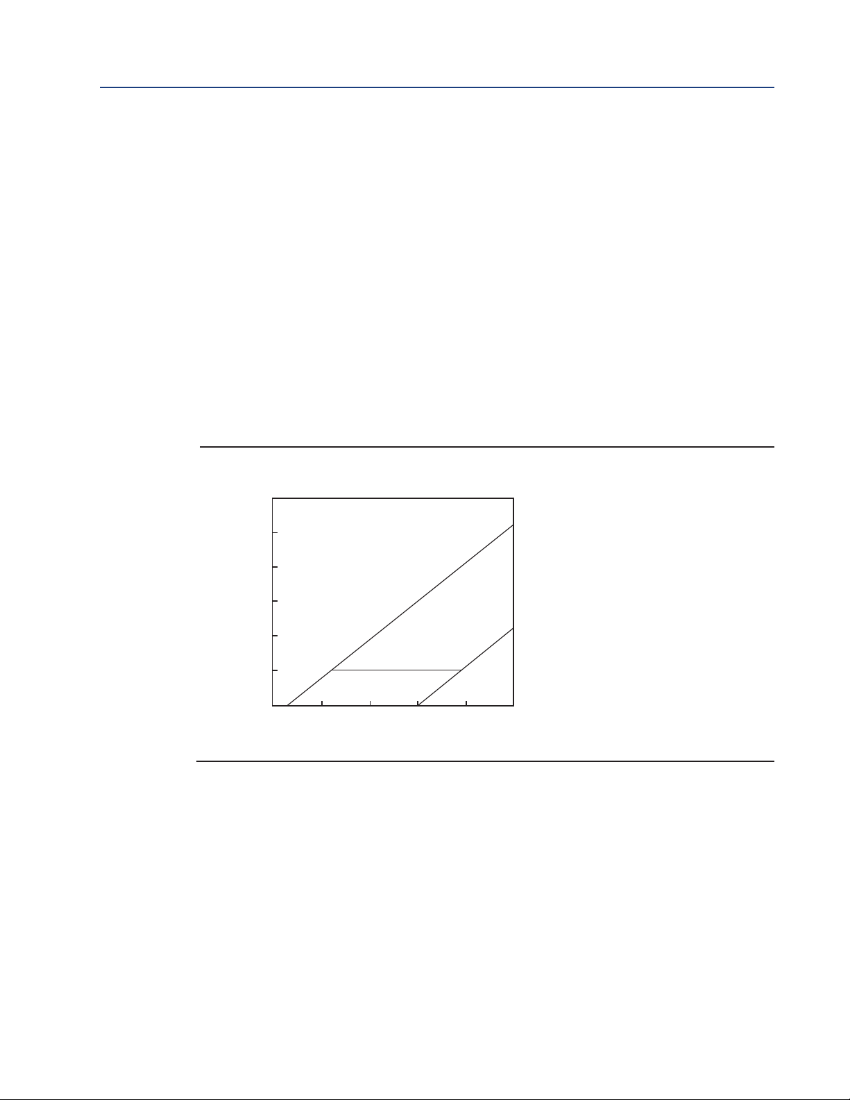
Power and Load Requirements:Supply voltage at the transmitter terminals should be at least 12.7 Vdc. Power supply voltage should cover the voltage drop on the cable plus the external load resistor required for HART communications (250 Ω minimum). Minimum power supply voltage is 12.7 Vdc. Maximum power supply voltage is 42.4 Vdc (30 Vdc for intrinsically safe operation). The graph shows the supply voltage required to maintain 12 Vdc (upper line) and 30 Vdc (lower line) at the transmitter terminals when the current is 22 mA.

FIGURE 2-1. Load/Power Supply Requirements

Analog Outputs: Two-wire loop powered (Output 1 only). Two 4-20 mA electrically isolated cur-

rent outputs (Output 2 must be externally powered). Superimposed HART digital signal on Output 1. Fully scalable over the operating range of the sensor.

Weight/Shipping Weight: 2 lbs/3 lbs (1 kg/1.5 kg)

Specifications 5

Page 16

Section 2: Description and Specifications Reference Manual

March 2020 00809-0100-3166

2.3

2.3.1

2.3.2

pH/ORP (Codes – P)

For use with any standard pH or ORP sensor. SMART pH sensor with SMART pre-amplifiers from Rosemount. Measurement choices are pH, ORP, or Redox. The automatic buffer recognition feature uses stored buffer values and their temperature curves for the most common buffer standards available worldwide. The transmitter will recognize the value of the buffer being measured and perform a self stabilization check on the sensor before completing the calibration. Manual or automatic temperature compensation is menu selectable. Change in pH due to process temperature can be compensated using a programmable temperature coefficient.

Performance Specifications - Transmitter (pH input)

Measurement Range [pH]: 0 to 14 pH Accuracy: ±0.01 pH Buffer recognition: NIST, DIN 19266, JIS 8802, and BSI. Input filter: Time constant 1 - 999 sec, default 4 sec. Response time: 5 seconds to 95% of final reading Recommended Sensors for pH:

All standard pH sensors. Supports SMART pH sensors from Rosemount.

Performance Specifications - Transmitter (ORP input)

Measurement Range [ORP]: -1400 to +1400 mV Accuracy: ± 1 mV Input filter: Time constant 1 - 999 sec, default 4 sec. Response time: 5 seconds to 95% of final reading Recommended Sensors for ORP: All standard ORP sensors

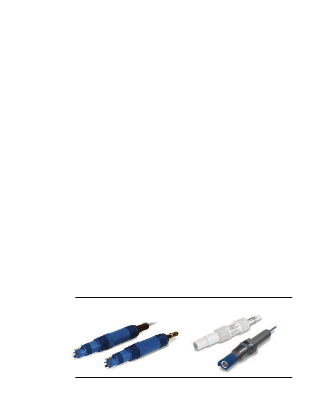
FIGURE 2-2. General purpose and high performance pH sensors 3900, 396PVP and 3300HT

6 Specifications

Page 17

Reference Manual Section 2: Description and Specifications

00809-0100-3166 March 2020

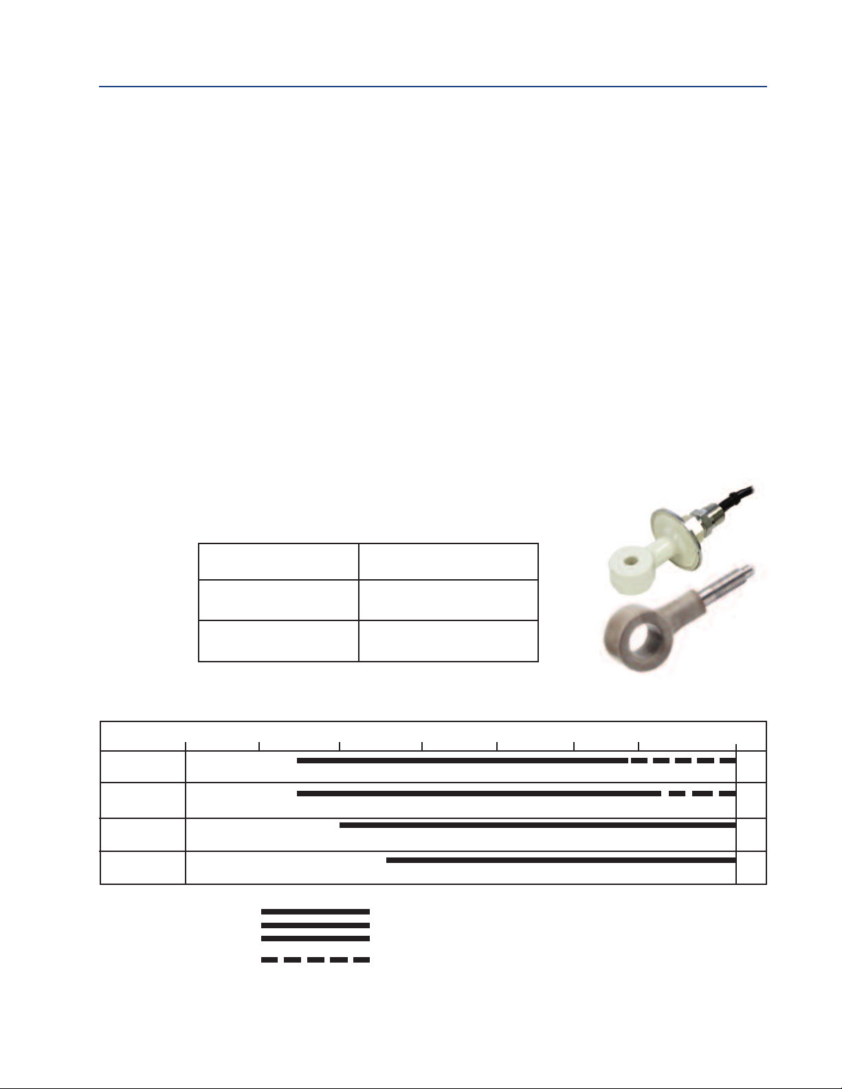
2.4

2.4.1

Contacting Conductivity (Codes – C)

Measures conductivity in the range 0 to 600,000 µS/cm (600mS/cm). Measurement choices are conductivity, resistivity, total dissolved solids, salinity, and % concentration. In addition, the “Custom Curve” feature allows users to define a three to five point curve to measure ppm, %, or a no unit variable. The % concentration selection includes the choice of five common solutions (012% NaOH, 0-15% HCl, 0-20% NaCl, and 0-25% or 96-99.7% H2SO4). The conductivity concentration algorithms for these solutions are fully temperature compensated. Three temperature compensation options are available: manual slope (X% / °C), high purity water (dilute sodium chloride), and cation conductivity (dilute hydrochloric acid). Temperature compensation can be disabled, allowing the transmitter to display raw conductivity. For more information concerning the use of the contacting conductivity sensors, refer to the product data sheets.

Note: The 410VP 4-electrode high-range conductivity sensor is compatible with the 1066.

Performance Specifications

Temperature specifications:

Temperature range 0-200 °C

Temperature Accuracy, Pt-1000, 0-50 °C

Temperature Accuracy, Pt-1000, Temp. > 50 °C

± 0.1 °C

± 0.5 °C

ENDURANCETMseries of

conductivity sensors

Input filter: Time constant 1 - 999 sec, default 2 sec. Response time: 3 seconds to 95% of final reading using the default input filter Salinity: Uses Practical Salinity Scale Total Dissolved Solids: Calculated by multiplying conductivity at 25 °C by 0.65

Table 2-1. Performance Specifications: Recommended Range – Contacting Conductivity

Cell 0.01S/cm 0.1µS/cm 1.0µS/cm 10µS/cm 100µS/cm 1000µS/cm 10mS/cm 100mS/cm 1000mS/cm Constant

0.01

0.1

1.0

4-electrode

Linearity for Standard

Cable ≤ 50 ft (15 m)

Specifications 7

0.01µS/cm to 200µS/cm

0.1µS/cm to 2000µS/cm

1 µS/cm to 20mS/cm

±0.6% of reading in recommended range

±2% of reading outside high recommended range

±5% of reading outside low recommended range

±4% of reading in recommended range

200µS/cm to 2000µS/cm

2000µS/cm to 20mS/cm

20mS/cm to 200mS/cm

2µS/cm to 1400mS/cm

Page 18

Section 2: Description and Specifications Reference Manual

March 2020 00809-0100-3166

2.4.2

2.5

2.5.1

Recommended Sensors for Conductivity

All Rosemount 400 series conductivity sensors (Pt 1000 RTD) and 410VP 4-electrode sensor.

Toroidal Conductivity (Codes – T)

Measures conductivity in the range of 1 µS/cm to 2,000,000 µS/cm (2 S/cm). Measurement choices are conductivity, resistivity, total dissolved solids, salinity, and % concentration. The % concentration selection includes the choice of five common solutions (0-12% NaOH, 0-15% HCl, 0-20% NaCl, and 025% or 96-99.7% H2SO4). The conductivity concentration algorithms for these solutions are fully temperature compensated. For other solutions, a simple-to-use menu allows the customer to enter his own data. The transmitter accepts as many as five data points and fits either a linear (two points) or a quadratic function (three to five points) to the data. Reference temperature and linear temperature slope may also be adjusted for optimum results. Two temperature compensation options are available: manual slope (X% / °C) and neutral salt (dilute sodium chloride). Temperature compensation can be disabled, allowing the transmitter to display raw conductivity. For more information concerning use of the toroidal conductivity sensors, refer to the product data sheets.

Performance Specifications

Temperature specifications:

High performance 225 Toroidal &

226 Conductivity sensors

Temperature range -25 to 210 °C (-13 to 410 °F)

Temperature Accuracy, Pt-100, -25 to 50 °C

Temperature Accuracy, Pt-100, 50 to 210 °C

± 0.5 °C

± 1 °C

Repeatability: ±0.25% ±5 µS/cm after zero cal

TABLE 2-2. Performance Specifications: Recommended Range – Toroidal Conductivity

Model 1µS/cm 10µS/cm 100µS/cm 1000µS/cm 10mS/cm 100mS/cm 1000mS/cm 2000mS/cm

226

225 & 228

242

222 (1in & 2in)

Loop Performance

(Following Calibration)

50µS/cm to 500mS/cm

50µS/cm to 1500mS/cm

100µS/cm to 2000mS/cm

500µS/cm to 2000mS/cm

226: ±1% of reading ±5µS/cm in recommended range 225 & 228: ±1% of reading ±15 222, 242: ±4% of reading ±5mS/cm in recommended range

225, 226 & 228: ±5% of reading outside high recommended range

µS/cm in recommended range

500mS/cm to 2000mS/cm

1500mS/cm to 2000mS/cm

8 Specifications

Page 19

Reference Manual Section 2: Description and Specifications

00809-0100-3166 March 2020

Input filter: time constant 1 - 999 sec, default 2 sec.

esponse time: 3 seconds to 95% of final reading

R Salinity: Uses Practical Salinity Scale Total Dissolved Solids: Calculated by multiplying conductivity at 25 °C by 0.65

2.5.2

2.6

2.6.1

2.6.2

Recommended Sensors for Conductivity

All Rosemount submersion/immersion and flow-through toroidal sensors.

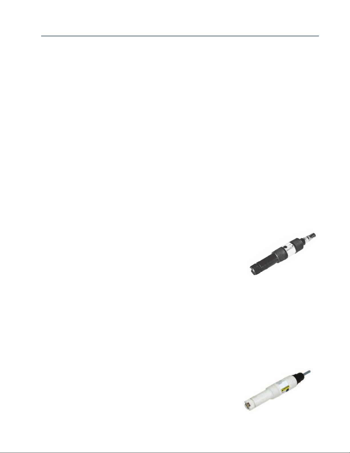
Chlorine (Codes – CL)

Free and Total Chlorine

The 1066 is compatible with the 499ACL-01 free chlorine sensor and the 499ACL-02 total chlorine sensor. The 499ACL-02 sensor must be used with the TCL total chlorine sample conditioning system. The 1066 fully compensates free and total chlorine readings for changes in membrane permeability caused by temperature changes. For free chlorine measurements, both automatic and manual pH correction are available. For automatic pH correction select an appropriate pH sensor. For more information concerning the use and operation of the amperometric chlorine sensors and the TCL measurement system, refer to the product data sheets.

Performance Specifications

Resolution: 0.001 ppm or 0.01 ppm – selectable Input Range: 0nA – 100 µA Automatic pH correction for Free Chlorine: (user selectable for code -CL): 6.0 to 10.0 pH Temperature compensation: Automatic (via RTD) or manual (050 °C). Input filter: Time constant 1 - 999 sec, default 5 sec. Response time: 6 seconds to 95% of final reading

499ACL-01

Chlorine sensor

2.6.3

2.6.4

Specifications 9

Recommended Sensors

Chlorine: 499ACL-01 Free Chlorine or 499ACL-02Total Residual Chlorine pH: These pH sensors are recommended for automatic pH correction of free chlorine readings: 3900-02-10, 3900-01-10, and 3900VP-02-10.

Monochloramine

The 1066 is compatible with the 499A CL-03 Monochloramine sensor. The 1066 fully compensates readings for changes in membrane permeability caused by temperature changes. Because monochloramine measurement is not affected by pH of the process, no pH sensor or correction is required. For more information concerning the use and operation of the amperometric chlorine sensors, refer to the product data sheets.

Page 20

Section 2: Description and Specifications Reference Manual

March 2020 00809-0100-3166

2.6.5

2.6.6

2.7

2.7.1

Performance Specifications

esolution: 0.001 ppm or 0.01 ppm – selectable

R Input Range: 0nA – 100µA Temperature compensation: Automatic (via RTD) or manual (0-50 °C). Input filter: Time constant 1 - 999 sec, default 5 sec. Response time: 6 seconds to 95% of final reading

Recommended Sensors

Rosemount 499ACL-03 Monochloramine sensor

Dissolved Oxygen (Codes –DO)

The 1066 is compatible with the 499ADO, 499ATrDO, Hx438, Gx438 and Bx438 dissolved oxygen sensors and the 4000 percent oxygen gas sensor. The 1066 displays dissolved oxygen in ppm, mg/L, ppb, µg/L, % saturation, % O2in gas, ppm O2in gas. The transmitter fully compensates oxygen readings for changes in membrane permeability caused by temperature changes. Automatic air calibration, including salinity correction, is standard. The only required user entry is barometric pressure. For more information on the use of amperometric oxygen sensors, refer to the product data sheets.

Performance Specifications

2.7.2

2.8

2.8.1

2.8.2

Resolution: 0.01 ppm; 0.1 ppb for 499A TrDO sensor (when O2<1.00 ppm); 0.1% Input Range: 0nA – 100 µA Temperature Compensation: Automatic (via RTD) or manual (0-50 °C). Input filter: Time constant 1 - 999 sec, default 5 sec. Response time: 6 seconds to 95% of final reading

Recommended Sensors

Rosemount amperometric membrane and steam-sterilizable sensors listed above

Dissolved Oxygen 499ADO sensor with Variopol connection

Ozone (Codes –OZ)

The 1066 is compatible with the 499AOZ sensor. The 1066 fully compensates ozone readings for changes in membrane permeability caused by temperature changes. For more information concerning the use and operation of the amperometric ozone sensors, refer to the product data sheets.

Performance Specifications

Resolution: 0.001 ppm or 0.01 ppm – selectable Input Range: 0nA – 100A Temperature Compensation: Automatic (via RTD) or manual (0-35 °C) Input filter: Time constant 1 - 999 sec, default 5 sec. Response time: 6 seconds to 95% of final reading

Recommended Sensors

Dissolved Ozone

499AOZ sensors with

Variopol connection

Rosemount 499A OZ ozone sensor

10 Specifications

Page 21

Reference Manual Section 2: Description and Specifications

00809-0100-3166 March 2020

2.9

Ordering Information

The 1066 2-Wire Transmitter is intended for the continuous determination of pH, ORP (Redox), conductivity, (both contacting and toroidal), and for measurements using membrane-covered amperometric sensors (oxygen, ozone, free and total chlorine, and monochloramine). For free chlorine measurements, which often require continuous pH correction a second input for a pH sensor is available. Two 4-20mA analog outputs are standard on HART units. The 1066 is compatible with SMART pH sensors from Rosemount. HART digital communications is standard and F

OUNDATION

Communication with the 1066 is through:

 Local keypad interface

 475 HART

 HART protocol version 7

FOUNDATION fieldbus

 AMS (Asset Management Solutions) Aware

 SMART Wireless THUM™Adapter

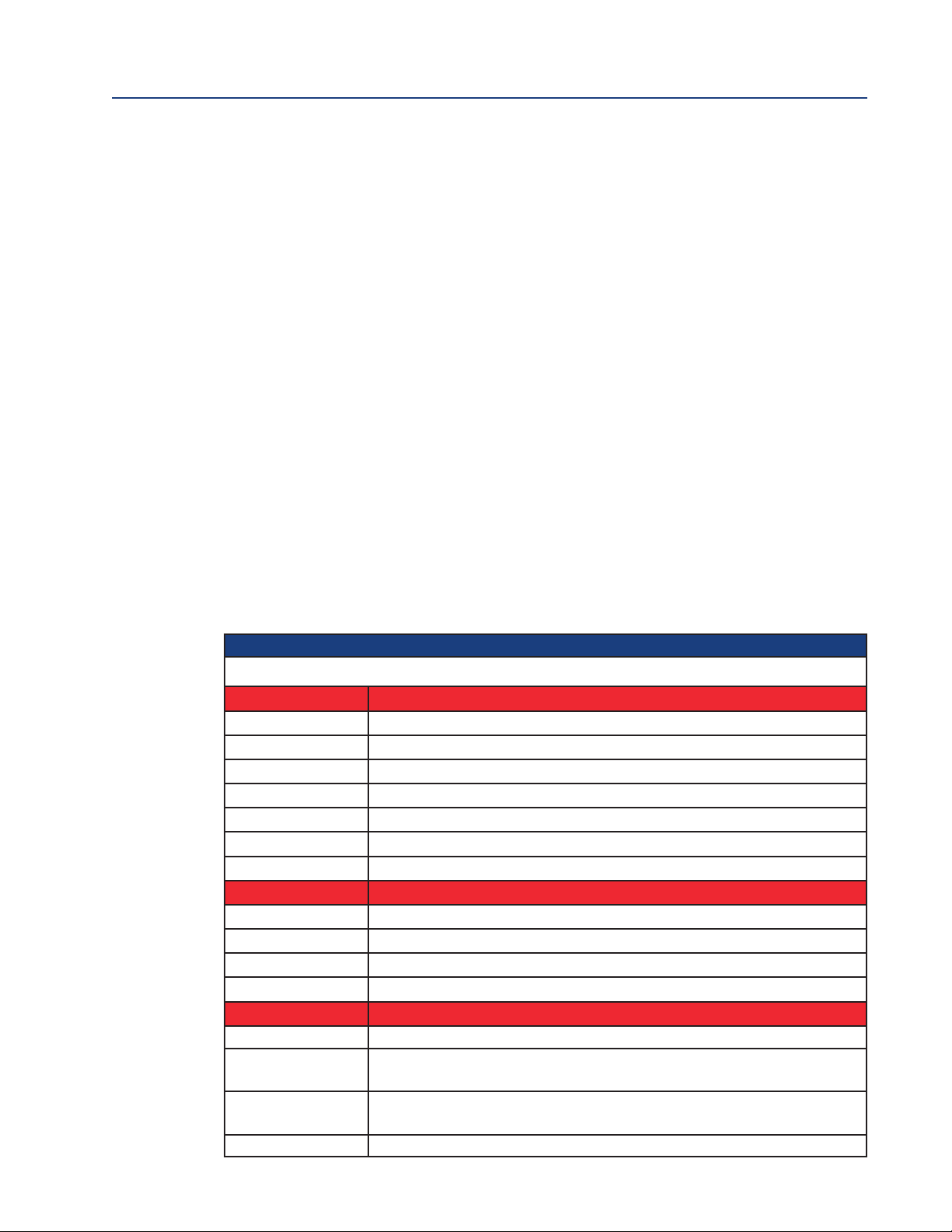
TABLE 2-3. Ordering Information

fieldbus digital communication is offered as an option.

and FO

UNDATION

fieldbus Communicator

Description

1066 pH/ORP, Conductivity, Chlorine, Oxygen, and Ozone 2-Wire Transmitter

Measurement

P pH/ORP

C Contacting Conductivity

T Toroidal Conductivity

CL Chlorine

DO Dissolved Oxygen

OZ Ozone

Communication

HT HART® Digital Communication Superimposed on 4-20mA Output

FF FOUNDATION™ fieldbus Digital Output

FI FOUNDATION™ fieldbus Digital Output with FISCO

Agency Approval

60 None Required

73 ATEX/IECEx Approved, Intrinsically Safe (safety barrier required)

FM Approved, Intrinsically Safe (appropriate sensor & safety barrier required), and Non-Incendive

CSA Approved , Intrinsically Safe (appropriate sensor & safety barrier required), and Non-Incendive

Specifications 11

Page 22

Section 2: Description and Specifications Reference Manual

March 2020 00809-0100-3166

12 Specifications

Page 23

Reference Manual Section 3: Installation

00809-0100-3166 March 2020

Section 3: Installation

3.1

3.2

Unpacking and inspection

Inspect the shipping container. If it is damaged, contact the shipper immediately for instructions. Save the box. If there is no apparent damage, unpack the container. Be sure all items shown on the packing list are present. If items are missing, notify Rosemount immediately.

Installation – General Information

1. Although the transmitter is suitable for outdoor use, installation is direct sunlight or in areas of extreme temperatures is not recommended unless a sunshield is used.

2. Install the transmitter in an area where vibration and electromagnetic and radio frequency interference are minimized or absent.

3. Keep the transmitter and sensor wiring at least one foot from high voltage conductors. Be sure there is easy access to the transmitter.

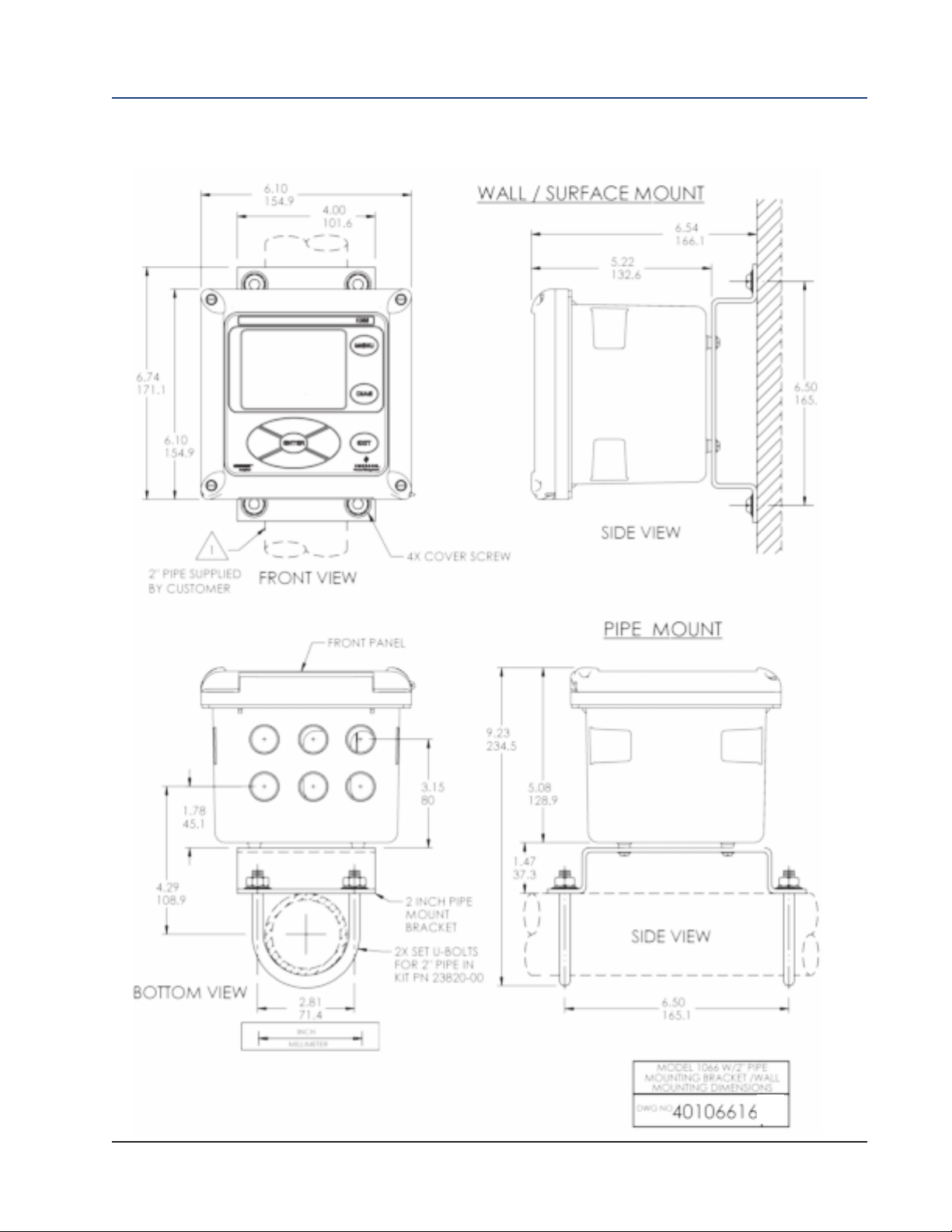
4. The transmitter is suitable for panel, pipe, or surface mounting.

5. The transmitter case has six 1/2-inch (PG13.5) conduit openings. Use separate conduit openings for the power/output cable, the sensor cable, and the other the sensor cable as needed (pH input for free chlorine with continuous pH correction).

6. Use weathertight cable glands to keep moisture out to the transmitter. If conduit is used, plug and seal the connections at the transmitter housing to prevent moisture from getting inside the instrument.

3.3

Preparing Conduit Openings

There are six conduit openings in all configurations of 1066. Conduit openings accept 1/2-inch conduit fittings or PG13.5 cable glands. To keep the case

watertight, block unused openings with Type 4X or IP66 conduit plugs. To maintain ingress protection for outdoor use, seal unused conduit holes with suitable conduit

plugs.

NOTE: Use watertight fittings and hubs that comply with your requirements. Connect the conduit hub to the conduit before attaching the fitting to the transmitter.

Electrical installation must be in accordance with the National Electrical Code (ANSI/NFPA-70) and/or any

other applicable national or local codes.

Installation 13

Page 24

Section 3: Installation Reference Manual

March 2020 00809-0100-3166

FIGURE 3-1. Panel Mounting Dimensions

14 Installation

Page 25

Reference Manual Section 3: Installation

00809-0100-3166 March 2020

FIGURE 3-2. Pipe and wall mounting dimensions (Mounting bracket PN: 23820-00)

Installation 15

Page 26

Section 3: Installation Reference Manual

March 2020 00809-0100-3166

16 Installation

Page 27

1500

1250

1000

750

500

250

Load, ohm s

with HART

com m uni cat i on

without HART

com m uni cat i on

12 18 24 30 36 42

545 ohm s

1364 ohm s

Pow er su pp l y vol tag e, Vdc

HART option

Reference Manual Section 4: Wiring

00809-0100-3166 March 2020

Section 4: Wiring

4.1

4.1.1

4.1.2

4.2

4.2.1

General

General Information

The 1066 is easy to wire. All wiring connections are located on the main circuit board. The front panel is hinged at the bottom. The panel swings down for easy access to the wiring locations.

Digital Communication

HART and FO units support Bell 202 digital communications over analog 4-20mA current output 1.

UNDATION

fieldbus communications are available as ordering options for 1066. HART

Power Supply/Current Loop – 1066 - HT

Power Supply and Load Requirements

Refer to Figure 4-1. The supply voltage must be at least 12.7 Vdc at the transmitter terminals.. The power supply must be able to cover the voltage drop on the cable as well as the load resistor (250 Ω minimum) required for HART communications. The maximum power supply voltage is 42.0 Vdc. For intrinsically safe installations, the maximum power supply voltage is 30.0 Vdc. The graph shows load and power supply requirements. The upper line is the power supply voltage needed to provide

12.7 Vdc at the transmitter terminals for a 22 mA current. The lower line is the power supply volt-

age needed to provide 30 Vdc for a 22 mA current. The power supply must provide a surge current during the first 80 milliseconds of startup. The maximum current is about 24 mA.

Wiring 17

For digital communications, the load must be at least 250 ohms. To supply the 12.7 Vdc lift off voltage at the transmitter, the power supply voltage must be at least 17.5 Vdc.

FIGURE 4-1. Load/Power Supply Requirements

Page 28

Section 4: Wiring Reference Manual

March 2020 00809-0100-3166

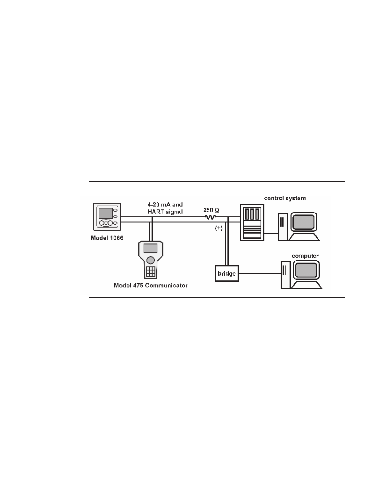
4.2.2

Power Supply-Current Loop Wiring

Refer to Figure 4-2.

Run the power/signal wiring through the opening nearest TB-2.

For optimum EMI/RFI protection:

1. Use shielded power/signal cable and ground the shield at the power supply.

2. Use a metal cable gland and be sure the shield makes good electrical contact with the gland.

3. Use the metal backing plate when attaching the gland to transmitter enclosure. The power/signal cable can also be enclosed in an earth-grounded metal conduit.

Do not run power supply/signal wiring in the same conduit or cable tray with loop power lines. Keep power supply/signal wiring at least 6 ft (2 m) away from heavy electrical equipment.

FIGURE 4-2. HART Communications

18 Wiring

Page 29

OUTPUT 2

TB5 TB3 TB2

TB4 TB1

+24V GND

GND

+24V

THUM

ANODE

CATHODE

RTN SNS

RTD IN

-V

REF SHLD

SENSOR WIRING

TB7

TB6

_ +

GND

SOL

SHLD pH

(OUTPUT1) LOOP PWR

4-20mA / -24VDC RETURN

4-20mA / +24VDC

INSTALL PLUGS IN ALL OTHER OPENINGS AS NEEDED

INNER ENCLOSURE

HINGE SIDE OF FRON T PANEL

TB7

/OUTPUT 2 REQUIRES EXTERNAL DC POWER.

TB6/

THUM T ERMINAL IS USED ONLY FOR

WIRELESS THUM ADA PT OR INSTALLATIONS

1066 HART CIRCUIT BO ARD (pH/CL/DO/OZ) ASS Y 24406-xx

HINGED PANEL

DW G NO.

40106613

Reference Manual Section 4: Wiring

00809-0100-3166 March 2020

4.2.3 Current Output wiring

The 1066 HART units are shipped with two 4-20mA current outputs. Current Output 1 is loop power; it is the HART communications channel. Current output 2 is available to report process temperature measured by the temperature sensing element or RTD within the sensor.

Wiring locations for the outputs are on the main board which is mounted on the hinged door of the instrument. Wire the output leads to the correct position on the main board using the lead markings (+/positive, -/negative) on the board.

Note: Twisted pairs are required to minimize noise pickup in the 4-20 mA current outputs. For high EMI/RFI environments, shielded sensor wire is required and recommended in all other installations.

FIGURE 4-3. 1066 HART Loop Power Wiring

Wiring 19

Page 30

Section 4: Wiring Reference Manual

March 2020 00809-0100-3166

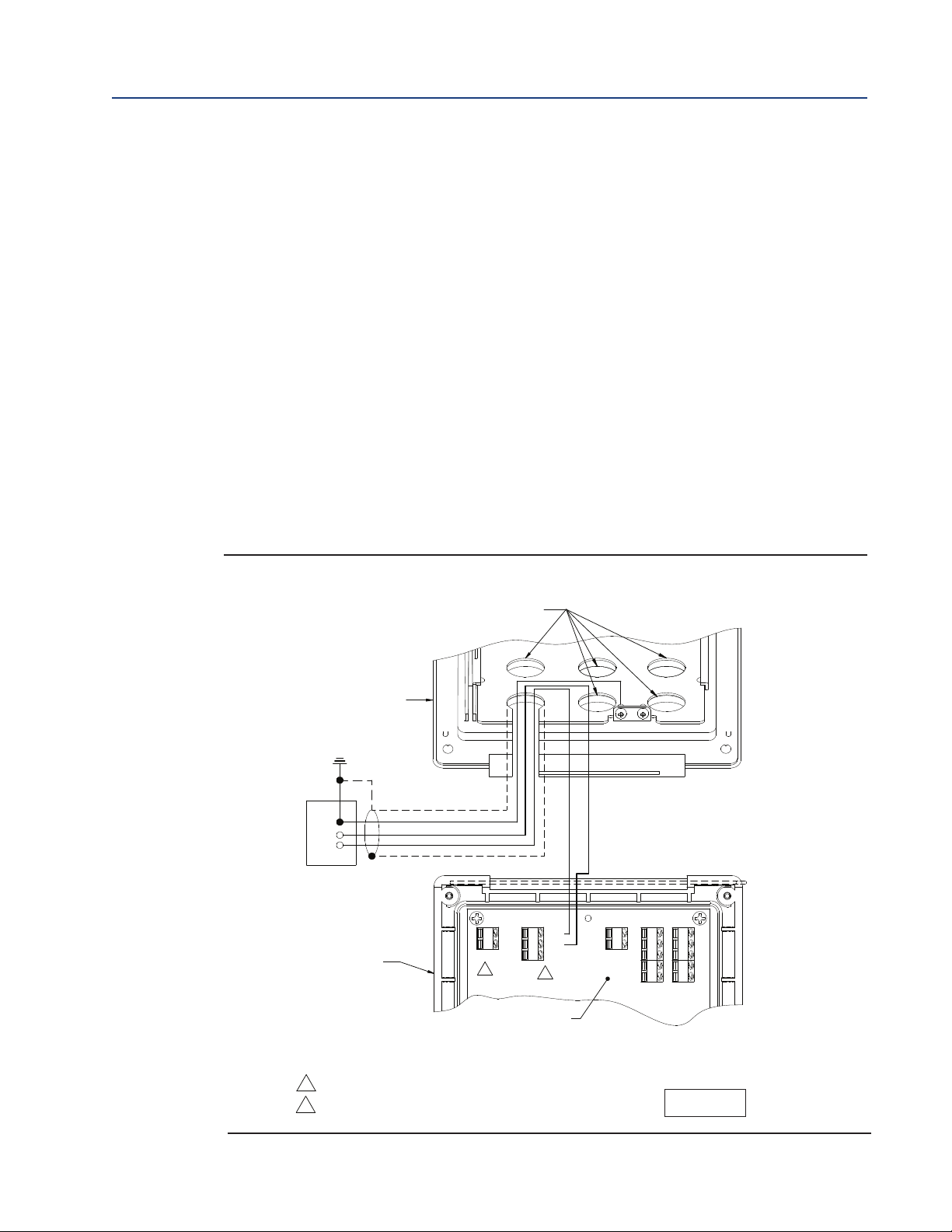
4.3

4.3.1

Power Supply Wiring For 1066-FF

Power Supply Wiring

Run the power/signal wiring through the opening nearest TB2. Use shielded cable and ground the shield at the power supply. To ground the transmitter, attach the shield to TB2-3.

Note: For optimum EMI/RFI immunity, the power supply/output cable should be shielded and enclosed in an earth-grounded metal conduit. Do not run power supply/signal wiring in the same conduit or cable tray with loop power lines. Keep power supply/signal wiring at least 6 ft (2 m) away from heavy electrical equipment.

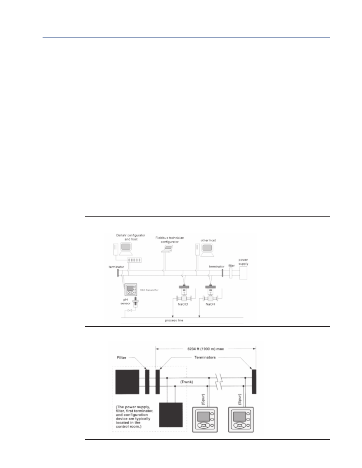
UNDATION

Figure 4-4 shows a 1066PFF being used to measure and control pH and chlorine levels in drinking

water. The figure also shows three ways in which Fieldbus communication can be used to read process variables and configure the transmitter.

FIGURE 4-4. Configuring 1066P Transmitter with FOUNDATION fieldbus

Fieldbus

FIGURE 4-5. Typical Fieldbus Network Electrical Wiring Configuration

20 Wiring

Page 31

DWG NO.

40106612

Reference Manual Section 4: Wiring

00809-0100-3166 March 2020

4.4

Sensor Wiring to Main Board

Wire the correct sensor leads to the main board using the lead locations marked directly on the board. Rosemount SMART pH sensors can be wired to the 1066 using integral cable SMART sensors or compatible VP8 pH cables. After wiring the sensor leads, carefully take up the excess sensor cable through the cable gland.

Keep sensor and output signal wiring separate from loop power wiring. Do not run sensor and power wiring in the same conduit or close together in a cable tray.

FIGURE 4-6. pH/ORP sensor wiring to the 1066 printed circuit board

Wiring 21

Page 32

Section 4: Wiring Reference Manual

DWG NO.

40106615

March 2020 00809-0100-3166

FIGURE 4-7. Contacting and Toroidal Conductivity sensor wiring to the 1066 circuit board

22 Wiring

Page 33

Reference Manual Section 4: Wiring

OUTPU T 2

(OUTPUT1) LOOP PWR

TB5 TB3 TB2

TB4 TB1

+24V GND

GND

+24V

THUM

ANODE

CATHO DE

RTN SNS

RTD IN

-V

REF

SHLD

SENSOR WIRING

TB7

TB6

GND

SOL

SHLD pH

HINGE SIDE OF FRONT PANEL

CHLORINE, OXYGEN , OZ ONE SENSOR WIRING

(FOLLOW RECOM M ENDED ORDER)

ANODE

CA THODE

TB5

/ANODE

& CATH ODE

RETURN SENSE

TB3

/RTD

SOLU TION GROU ND

TB2

/ SOLUT IO N

GROUND

RTD IN NO CONNECTION

NO CONNECTION

NOTE: A) TB1, TB4, TB6 AND TB7 NOT USED F O R OXYGEN AND OZONE SENSO R WIRING B) TB1, TB2 A ND TB4 MAY BE USED FOR p H SENSOR WIRING IF FREE CHLORINE MEASUREMENT REQ UIRES

LIVE pH INPU T.

1066 CIRCUIT BOARD ASSY 24406-xx

DWG NO.

40106611

00809-0100-3166 March 2020

FIGURE 4-8. Chlorine, oxygen, ozone sensor wiring to 1066 printed circuit board (1066-CL, 1066-DO,

066-OZ)

Wiring 23

Page 34

Section 4: Wiring Reference Manual

OUTPUT 2

B5 TB3 TB2

TB4 TB1

+24V GND

GND

+24V

THUM

NODE

CATHODE

RTN SNS

RTD IN

-V

REF

SHLD

GND

SOL

SHLD pH

SENSOR WIRING

TB7

TB6

_ +

RED / +VDC

YELLO W / OUTPUT 1 +24V

BLACK / OUTPUT 1 GND

GREEN / GROUND SCREW

W HITE

WIRE NUT

LOOP POWER/THUM

(OUTPUT1) LOOP PWR

4-20mA / -24VDC RETURN

4-20m A / +24VDC

TB7

/OUTPUT 2 REQUIRES EXTERNAL DC POWER.

TB6/

THUM TERMINAL IS USED ONL Y FOR WIRELESS THUM ADAPTOR INSTALLATIONS. 250 OHM RESISTOR IS PRE-INSTALLED IN-CIRCUIT.

3 SPLICE CONNECTOR - PROVIDED BY END USER.

INSTALL PLUGS IN ALL OTHER

OPENINGS AS NEE D ED

INNER ENCLOSURE

HINGE S IDE OF FRONT PANEL

WIRELESS

THUM

ADAPTOR

1066 HART CIRCUIT BOARD (pH/CL/DO/OZ) ASSY 24406-xx

DWG NO.

40106614

March 2020 00809-0100-3166

FIGURE 4-9. Power/Current Loop wiring with wireless THUM Adaptor

24 Wiring

Page 35

Reference Manual Section 4: Wiring

OUTPU T 2

TB5 TB3 TB2

TB4 TB1

+24V

GND

+24V

THUM

ANODE

CATHODE

RTN SNS

RTD IN

-V

REF SHLD

SENSOR WIRING

TB7

TB6

GND

SOL

SHLD pH

(OUTPUT1) LOOP PW R

4-20mA / -24VDC RETURN

4-20m A / +24VDC

INSTALL PLUGS IN ALL OTHER OPENINGS AS NEEDED

INNER ENCLOSURE

HINGE SIDE O F FR ONT PANEL

TB7

/OUTPUT 2 REQUIRES EXTERNAL DC POWER.

TB6/

THUM TERMINAL IS USED ONLY FOR

WIRELESS THUM ADAPTOR INSTALLATIONS

1066 HART CIRCUIT BOARD (pH/CL/DO/OZ) ASS Y 24406-xx

HINGED PANEL

DWG NO.

40106613

00809-0100-3166 March 2020

FIGURE 4-10. HART Loop Power Wiring

Wiring 25

Page 36

Section 4: Wiring Reference Manual

March 2020 00809-0100-3166

26 Wiring

Page 37

Reference Manual Section 4: Wiring

(



)

(

)

:

ARAM

RAN

(

ALLAT

RAW

)

RMI

ALS

...

RMI

ALS

...H

...

ALO

RMI

(

)

(

)

(

)

(

)

ABLE

ARAME

ABLE

(

...)

(



)

(

)

ABLE

(

L/D

066-AA-BB-C

LON G

AN D

AN C

O NN EC

O R

EXC

EED

DEV

G E

Y C

O N

O L

O C

G E

PPR

O VA

00809-0100-3166 March 2020

Section 5: Intrinsically Safe Installation

5.1

All Intrin sically Safe Installations

FIGURE 5-1. CSA Installation

Intrinsically Safe Installation 27

Page 38

Section 4: Wiring Reference Manual

SHLD

SOL

GND

TB6

TB7

SENSOR W IRING

SHLD

REF

RTD IN

SNS

RTN

CATHODE

ANO DE

THUM

GND

TB1

TB4

TB2TB3

TB5

LOOP PWR

(OUTPUT1)

OUTPUT 2

SHLD

SOL

GND

TB6

TB7

SENSOR W IRING

SHLD

REF

RTD IN

SNS

RTN

CATHODE

ANO DE

THUM

GND

TB1

TB4

TB2TB3

TB5

LOOP PWR

(OUTPUT1)

OUTPUT 2

SHLD

SOL

GND

TB6

TB7

SENSOR W IRING

SHLD

REF

RTD IN

SNS

RTN

CATHODE

ANO DE

THUM

GND

TB1

TB4

TB2TB3

TB5

LOOP PWR

(OUTPUT1)

OUTPUT 2

W ARNING- SUBSTITUTION OF CO M PONENTS M AY IM PAIR INTRINSIC SAFETY O R

SUITABILITY FOR DIVISION 2.

W ARNING- TO PREVENT IGNITION OF FLAM M ABLE OR COM BUSTIBLE ATMO SPHERES,

DISCONNECT POW ER BEFORE SERVICING.

ROSEMOUN T M O DEL 375 OR 475

FIELD CO M M UNICATOR REMOTE TRANSMITTER

INTERFACE FOR USE IN CLASS I AREA

(SEE NOTE 3 AND TABLE III)

PH SENSOR

CSA APPROVED DEVICE OR

SIM PLE APPARATUS

NI CLASS I, DIV 2

GRPS A-D

CLASS II, DIV 2

GRPS E-G

AM PEROM ETRIC SENSOR

CSA APPROVED DEVICE OR

SIM PLE APPARATUS

1066-CL/D O/OZ...O NLY

EITHER O R BOTH

MAY BE INSTALLED

ROSEMOUN T M O DEL 375 OR 475

FIELD CO M M UNICATOR REMOTE TRANSMITTER

INTERFACE FOR USE IN CLASS I AREA

(SEE NOTE 3 AND TABLE III)

LOAD

UNSPECIFIED

POW ER SUPPLY

30 VDC M AX FOR IS

24V TYPICAL

SAFETY BARRIER

(SEE NOTES 10 & 11)

SPLICE CONNECTOR

RED

SMART THUM

W IRELESS

ADAPTER

ALTERNATE POW ER CONN ECTION IF SM ART

THUM W IRELESS AD APTER IS USED

(SENSOR AND SECOND ANALOG O UTPUT

CONNECTION U NCHANGED FROM ABOVE)

ROSEMOUN T M O DEL 375 OR 475

FIELD CO M M UNICATOR REMOTE TRANSMITTER

INTERFACE FOR USE IN CLASS I AREA

(SEE NOTE 3 AND TABLE III)

AM PEROM ETRIC SENSOR

CSA APPROVED DEVICE

OR SIM PLE APPARATUS

1066-CL/D O/OZ...O NLY

EITHER O R

BOTH MAY BE

INSTALLED

OPTIO NAL

CSA APPROVED PREAMP THAT

MEETS REQUIREMENTS O F

NOTE 4

PH SENSOR

CSA APPROVED DEVICE OR

SIM PLE APPARATUS

RECOMM ENDED CABLE PN 9200273

(UNPREPED) PN 23646-01 (PREPPED)

10 CO ND, 2 SHIELDS, 24 AW G. SEE NOTE 2

ANALOG OUTPUT 2 ONLY AVAILABLE

ON 1066...HT...

ANALOG OUTPUT 2 ONLY AVAILABLE

ON 1066...HT...

LOAD

UNSPECIFIED POW ER SUPPLY

30 VDC M AX FOR INTRINSIC SAFETY (24 VDC TYPICAL)

17.5 VDC M AX. FOR FISCO OPTION

LOAD

UNSPECIFIED POW ER SUPPLY

30 VDC M AX FOR INTRINSIC SAFETY (24 VDC TYPICAL)

17.5 VDC M AX. FOR FISCO OPTION

SAFETY BARRIER

(SEE NOTES 2 & 8 FOR FISCO,

SEE NO TES 2, 8, 9 & 10

FOR ALL O THER OPTIONS.)

LOAD

UNSPECIFIED POW ER SUPPLY

30 VDC M AX FOR INTRINSIC SAFETY (24 VDC TYPICAL)

17.5 VDC M AX. FOR FISCO OPTION

SAFETY BARRIER

(SEE NOTES 2 & 8 FOR FISCO,

SEE NO TES 2, 8, 9 & 10

FOR ALL O THER OPTIONS.)

LOAD

SAFETY BARRIER

(SEE NOTES 2 & 8 FOR FISCO,

SEE NO TES 2, 8, 9 & 10

FOR ALL O THER OPTIONS.)

GREEN

BLACK

YELLOW

W HITE

N/C

O R

SAFETY BARRIER

(SEE NOTES 2 & 8 FOR FISCO,

SEE NO TES 2, 8, 9 & 10

FOR ALL O THER OPTIONS.)

UNSPECIFIED POW ER SUPPLY

30 VDC M AX FOR INTRINSIC SAFETY (24 VDC TYPICAL)

17.5 VDC M AX. FOR FISCO OPTION

IS CLASS I, GRPS A-D

CLASS II, GRPS E-G

CLASS III

REV

DW G NO

October 2017 00809-0100-3166

FIGURE 5-2. CSA Installation

28 Intrinsically Safe Installation

Page 39

Reference Manual Section 5: Intrinsically Safe Installation

OUTPUT2

TB2

TB1

LOOP PWR

DSHLD

DRV_A

RTN

DRV_B

RSHLD

RCV_A

SHLD

RTDIN

TB7

TB6

GND

+24V

THUM

RCV_B

SENSE

+24V

OUTPUT2

TB2

TB1

LOOP PWR

DSHLD

DRV_A

RTN

DRV_B

RSHLD

RCV_A

SHLD

RTDIN

TB7

TB6

GND

+24V

HUM

RCV_B

SENSE

OUTPUT 2

(OUTPUT1)

LOOP PWR

TB5

TB3 TB2

TB4

TB1

GND

THUM

ANO DE

CATHODE

RTN

SNS

RTD IN

REF

SHLD

SENSOR W IRING

TB7

TB6

GND

SOL

SHLD

W ARNING- SUBSTITUTION OF COM PONENTS M AY IM PAIR INTRINSIC SAFETY OR

SUITABILITY FOR DIVISION 2.

W ARNING- TO PREVENT IGNITION O F FLAMM ABLE O R CO M BUSTIBLE ATMOSPHERES,

DISCONNECT POW ER BEFORE SERVICING.

ROSEMOUN T M O DEL 375 OR 475

FIELD COM M UNICATOR REMOTE

TRANSMITTER INTERFACE FOR USE

IN CLASS I AREA

(SEE NOTE 3 AND TABLE III)

LOAD

IS CLASS I, GRPS A-D

CLASS II, GRPS E-G

CLASS III

NI CLASS I, DIV 2

GRPS A-D

CLASS II, DIV 2

GRPS E-G

ANALOG OUTPUT 2 ONLY

AVAILABLE ON 1066...HT...

APPROVED M ODEL 222, 225, 226 OR 228 TOROIDAL COND UCTIVITY SENSOR

MODELS 140, 141, 142, 150, 400, 400VP, 401, 402, 402VP, 403, 403VP, 404 &

410VP CONTACTING CONDUCTIVITY SENSOR

ANY SIM PLE APPARATUS W ITH LESS THAN 200 FEET OF ATTACHED CABLE

UNSPECIFIED POW ER SUPPLY

30 VDC M AX FOR INTRINSIC

SAFETY (24 VDC TYPICAL)

17.5 VDC M AX. FOR FISCO OPTION

SAFETY BARRIER

(SEE NOTES 2 & 8 FOR FISCO,

SEE NOTES 2, 8, 9 & 10

FOR ALL OTHER OPTIONS.)

LOAD

UNSPECIFIED POW ER SUPPLY

30 VDC M AX FOR INTRINSIC

SAFETY (24 VDC TYPICAL)

17.5 VDC M AX. FOR FISCO OPTION

SAFETY BARRIER

(SEE NOTES 2 & 8 FOR FISCO,

SEE NOTES 2, 8, 9 & 10

FOR ALL OTHER OPTIONS.)

PH SENSOR

CSA APPROVED DEVICE O R

SIM PLE APPARATUS

AM PEROM ETRIC SENSOR

CSA APPROVED DEVICE O R

SIM PLE APPARATUS

1066-CL/D O/OZ...ONLY

EITHER OR BOTH

MAY BE INSTALLED

ANALOG OUTPUT 2 ONLY AVAILABLE ON 1066...HT...

ANALOG OUTPUT 2 ONLY AVAILABLE ON 1066....HT...

O R

APPROVED M ODEL 222, 225, 226 OR 228 TOROIDAL COND UCTIVITY SENSOR

MODELS 140, 141, 142, 150, 400, 400VP, 401, 402, 402VP, 403, 403VP, 404 &

410VP CONTACTING CONDUCTIVITY SENSOR

ANY SIM PLE APPARATUS W ITH LESS THAN 200 FEET OF ATTACHED CABLE

1066C... ENTITY OUTPUT PARAMETERS: Voc = 4.75V, Isc = 676.93m A, Pmax = 258m W

THE 1066C IS CERTIFIED AS A SYSTEM FOR USE W ITH M ODELS 140, 141, 142, 150, 400, 400VP, 401, 402, 402VP, 403, 403VP, 404 & 410VP CONTACTING

CONDUCTIVITY SENSORS, OR ANY SIM PLE APPARATUS W ITH < 200 FEET OF CABLE.

THE 1066T... IS CERTIFIED AS A SYSTEM FOR USE W ITH THE M ODELS 222, 225, 226 & 228 TOROIDAL CONDUCTIVITY SENSORS, OR ANY SIM PLE APPARATUS

W ITH < 200 FEET OF CABLE.

17 18

15 16 17

17 18

REV

DW G NO

00809-0100-3166 March 2020

FIGURE 5-3. CSA Installation

Intrinsically Safe Installation 29

Page 40

Section 5: Intrinsically Safe Installation Reference Manual

TABLE III

19. A 1066 W ITH THE -FI O PTIO N M AY BE INSTA LLED PER THE FISCO INSTRUCTIO NS O R PER THE INTRINSIC ALLY SAFE IN STRUC TIO NS O N THIS DRAW ING .

IN STALLATIO N TO BE IN AC C O RDA N C E W ITH THE NA TIO NA L ELEC TRIC AL C O D E.16 N O N -INC END IVE FIELD W IRIN G METHO D S M A Y BE USED FOR C O NN EC TIN G SENSORS TO THE INSTRUM ENT. A TTA C H ED SENSO RS M UST BE FM A PPRO V ED

D IVISIO N 2 W IRING M ETHO D PER THE N EC (EXCLUDIN G NO N IN C END IV E FIELD W IRIN G ).

14. M ETAL C O ND UIT IS NO T REQ UIRED FOR INTRINSIC A LLY SAFE IN STA LLATIO N S. HO W EVER, IF C O NDU IT IS USED, BO N DING BETW EEN C O NDU IT IS N O T

AUTOM A TIC A N D M UST BE PRO V ID ED AS PART O F THE INSTA LLATIO N.

13. N O REVISIO N TO DRAW ING W ITHO UT PRIO R FM A PPRO V AL. A G ENC Y C O N TROLLED D O C UM ENT.

12. THE ASSOC IATED APPA RA TUS M UST BE FM A PPRO V ED AN D M UST BE RESISTIVELY LIM ITED HAV IN G LINEAR O UTPUTS.

11. C O NTROL EQ UIPM ENT C O N N EC TED TO A SSOCIATED A PPA RATUS M UST NO T USE O R G EN ERATE M O RE THAN 250 Vrm s O R V dc.

9. THE IN TRIN SICALLY SAFE ENTITY C O N C EPT A LLO W S INTERC O N NECTIO N O F IN TRIN SIC ALLY SAFE D EVIC ES W ITH ASSOC IATED APPA RA TUS W HEN

THE FO LLO W IN G IS TRUE:

FIELD D EVIC E IN PUT ASSO C IA TED APPARA TUS O UTPUT

8. RESISTAN C E BETWEEN IN TRIN SIC ALLY SAFE G RO UN D AND EARTH G RO UN D M UST BE LESS THAN 1.0 O hm .

7. DUST-TIG HT CO N D UIT SEAL M UST BE USED W HEN IN STALLED IN CLASS II A N D C LASS III ENVIRO N M ENTS.

6. C O NTAC TIN G C O NDUC TIVITY SENSORS, AM PERO M ETRIC AN D pH SENSO RS W ITHO UT PREAM PS SHALL M EET THE REQ UIREM ENTS O F SIM PLE APPARA TUS

AS D EFIN ED IN AN SI/ISA RP12.6 A ND THE N EC , A N SI/NFPA 70. THEY C A N N O T G EN ERATE N O R STO RE M O RE THAN 1.5 V, 100 m A , 25 m W O R A PA SSIVE

CO M PO NEN T THAT DO ES NO T D ISSIPATE M O RE THAN 1.3W .

4. W HEN C O NNEC TIO NS A RE M A DE TO 1066...H T... O PTIO N A NALOG O UTPUT 2 (TB7-1 & -2), SEPARA TE W IRIN G AND A SEC O N D BA RRIER ARE

REQ UIRED . THE W IRIN G FROM EAC H BARRIER M UST BE IN STALLED AS SEPARATE INTRINSIC ALLY SAFE C IRC U ITS IN AC C O RD A NC E W ITH THE N A TIO N A L

ELECTRICAL C O DE.

3. INTRINSIC A LLY SAFE A PPA RATUS (M O DEL 1066, SM ART THUM W IRELESS A D A PTER, M O D EL 375, 475) AN D A SSOC IATED A PPARATUS (SAFETY BARRIER)

OR G REATER THA N THE V O LTAG E (Voc O R Vt) A N D C URRENT (Isc O R It) W HIC H CAN BE D EVELOPED BY THE ASSO C IA TED APPARA TUS (SAFETY BARRIER).

IN ADD ITIO N, THE M A XIM UM U NPRO TECTED C APAC ITAN C E (Ci) A ND INDU C TANC E (Li) O F THE IN TRIN SIC ALLY SAFE APPARA TUS, INC LUDING

INTERCO NNEC TIN G W IRIN G , M UST BE EQ UA L O R LESS THA N THE C APA C ITAN C E (Ca) AN D IN D UC TAN C E (La) W HIC H C A N BE SAFELY C O N N EC TED TO

THE A PPARATUS. (REF. TABLES I, II AN D III).

2. THE M O DEL 1066-C /T HA S SYSTEM APPRO VA L FOR USE W ITH M O DELS 222, 225, 226 & 228 TORO ID A L SENSO RS O R 140, 141, 142, 150, 400, 401, 402,

1066 M O D ELS W ITH P/L/D/Z OPTIO NS H AVE O UTPUT ENTITY PA RA M ETERS W HIC H A LLO W THE USE O F VA RIO US SENSORS W H IC H M AY

TO THE SENSOR TERMINA LS D O NO T EXCEED THE V ALUES SPECIFIED IN TABLE I W HERE:

1. ANY SIN G LE SHUNT ZENER DIO D E SAFETY BA RRIER A PPRO V ED BY FM HAV IN G THE FO LLO W IN G O UTPUT PARAM ETERS: SUPPLY/SIG NAL TERM IN A LS TB6-1

AND 2 FO R FIELDBUS O PTIO N O R TB6-1, 2 A ND 3 FO R HA RT O PTIO N. A LSO TB7-1 AN D 2 IF A NALO G O UTPUT 2 IS USED.

APPRO VED M O DELS 1066-AA-BB-CC XMTR

20. THE FISCO C O N C EPT A LLO W S INTERCO NNEC TIO N O F IN TRIN SICALLY SAFE APPARA TUS TO A SSOC IA TED APPARA TUS N O T SPECIA LLY EXAM IN ED

DELIV ERED BY THE ASSO C IA TED APPARA TUS, CO N SIDERIN G FAULTS A ND APPLICABLE FAC TORS. IN AD D ITIO N, THE M A XIM UM UNPRO TECTED

CAPAC ITAN C E (Ci) A N D THE IN D UC TAN C E (Li) O F EA C H APPARA TUS (OTHER THAN THE TERM IN A TIO N) C O N NECTED TO THE FIELDBUS M UST BE

LESS THAN O R EQ UAL TO 5nF and 10

H RESPECTIV ELY.

IN EA C H SEG M ENT O NLY O NE AC TIVE D EVIC E, NO RM ALLY THE ASSO C IA TED APPA RA TUS, IS ALLO W ED TO PRO VID E THE NEC ESSARY ENERG Y

FO R THE FIELDBUS SYSTEM . THE VO LTA G E Uo (O R V oc O R V t) O F THE A SSOC IATED A PPARATUS IS LIM ITED TO A RA NG E O F 14 V TO 24 Vd c. ALL

OTHER EQ UIPM ENT C O N N EC TED TO THE BUS C ABLE HAS TO BE PA SSIVE, M EAN ING THAT THEY ARE N O T ALLO W ED TO PRO VID E ENERG Y TO THE

SYSTEM , EXCEPT A LEAKA G E C URRENT O F 50

FOR EACH C O N N ECTED DEVIC E. SEPARATELY PO W ERED EQUIPM ENT NEEDS G ALVAN IC

ISOLATIO N TO A SSURE THAT THE IN TRIN SICALLY SAFE FIELDBUS C IRC UIT REM A IN S PASSIV E.

THE C A BLE USED TO INTERCO NNEC T DEVICES N EEDS TO H AVE THE PARA M ETERS IN THE FOLLO W ING RAN G E:

AT EAC H END O F THE TRUNK C ABLE AN A PPRO VED IN FALLIBLE LINE TERM IN ATIO N W ITH THE FOLLO W ING PA RA M ETERS IS SUITABLE:F ON E O F THE ALLOW ED TERMINA TIO NS M IG HT ALREAD Y BE INTEG RA TED IN THE ASSO C IA TED APPARA TUS. THE N UM BER O F PASSIVE A PPARATUS

CO N N EC TED TO THE BUS SEGM ENT IS NO T LIM ITED

DUE TO I.S. REASO N S. IF THE A BO V E RULES ARE

RESPECTED , UP TO A TO TAL LENG TH O F 1000 m

(SUM O F TRUNK AND ALL SPUR C A BLES) O F C ABLE

IS PERM ITTED. THE IND UC TANC E AN D THE

CAPAC ITAN C E O F THE C A BLE W ILL NO T IM PA IR THE

INTRINSIC SAFETY O F THE INSTALLA TIO N .

GAS

GROUPS

OUTPUT PARAMETERS

FF/FI

2.22

0.795

5.86

II B

15.5 3.17 23.5

II A

68.9 6.36

OUTPUT

PARAMETERS

Uo (Vt) Volts

10.69 11.33

211.2 77.77

250

110.12

MODEL NO.

SIGNAL

MODEL NO.

NO TES: UNLESS OTHERW ISE SPECIFIED

SCALE: 1:1

W EIG H T:

SIZE

DW G NO

SHEET 1 OF 3

1400670

REV

AG ENC Y C O NTRO LLED D O CUM ENT

AN Y C HA NG E W ILL REQ UIRE

C ERTIFIC A TIO N AG ENC Y

SUBM ITTA L/A PPRO VA L

March 2020 00809-0100-3166

FIGURE 5-6. FM installation

30 Intrinsically Safe Installation

Page 41

Reference Manual Section 5: Intrinsically Safe Installation

OUTPUT 2

(OUTPUT1)

LOOP PWR

TB5

TB3 TB2

TB4

TB1

+24V

GND

+24V

THUM

ANODE

CATHODE

RTN

SNS

RTD IN

-V

REF

SHLD

SENSOR W IRING

TB7

TB6

GND

SOL

SHLD

OUTPUT 2

(OUTPUT1)

LOOP PWR

TB5

TB3 TB2

TB4

TB1

+24V

GND

+24V

THUM

ANODE

CATHODE

RTN

SNS

RTD IN

-V

REF

SHLD

SENSOR W IRING

TB7

TB6

GND

SOL

SHLD

OUTPUT 2

(OUTPUT1)

LOOP PWR

TB5

TB3 TB2

TB4

TB1

+24V

GND

+24V

THUM

ANODE

CATHODE

RTN

SNS

RTD IN

-V

REF

SHLD

SENSOR W IRING

TB7

TB6

GND

SOL

SHLD

LOA D

M ULTIPLE D EVIC ES

(N UM BER IS LIM ITED BY

THE REQ UIREM ENT TO

M EET ALL O THER

FIELDBUS I.S. & FISCO

REQ UIREM ENTS FOR THE

NETW O RK.)

O PTIO NA L FOR

FIELDBUS /FISCO

INSTALLA TIO N S

O PTIO NA L FOR

FIELDBUS /FISCO

INSTALLA TIO N S

O R

W HITE

YELLOW

GREEN

SAFETY BARRIER

( SEE N O TES 2, 8, 9 & 10

FOR ALL O THER O PTIO N S.)

UNSPECIFIED PO W ER SUPPLY

30 V DC M A X FO R IN TRIN SIC SAFETY

(24 VDC TYPIC A L)

LOA D

SAFETY BARRIER

(SEE N O TES 2,8,20

FOR FISCO IN STALLA TIO N S,

SEE NO TES 2, 8, 9 & 10

FOR ANY O THER)

UNSPECIFIED PO W ER SUPPLY

30 V DC M A X FO R IN TRIN SIC

SAFETY (24 VD C TYPIC AL)

17.5 V DC M A X. FO R FISCO O PTIO N

LOA D

AN A LOG O UTPUT 2 O N LY AV A ILABLE

O N 1066...HT...

AN A LOG O UTPUT 2 O N LY AV A ILABLE

O N 1066...HT...

EITHER O R

BO TH M AY BE

INSTALLED

1066-C L/DO /OZ... O N LY

AM PERO M ETRIC SENSO R

FM A PPRO V ED DEVICE

O R SIM PLE APPA RA TUS

RO SEM O UNT M O D EL 375 O R 475

FIELD C O M M UNIC ATO R REM O TE TRAN SM ITTER

INTERFA C E FO R USE IN C LASS I AREA

(SEE N O TE 3 AN D TABLE III)

(SENSO R A N D SECO N D ANALO G O UTPUT

C O N N EC TIO N U NC HA N G ED FRO M A BO VE)

ALTERNATE POW ER CONNECTIO N IF SMART

THUM W IRELESS ADAPTER IS USED

RED

SAFETY BARRIER

(SEE N O TES 10 & 11)

UNSPECIFIED

PO W ER SUPPLY

30 V DC M A X FO R IS

24V TYPIC A L

LOA D

1066-C L/DO /OZ... O N LY

HAZARDOUS AREA

IS C LASS I, G RPS A -D

C LASS II, G RPS E-G

C LASS III

NI CLASS I, D IV 2

G RPS A-D

CLASS II, D IV 2

G RPS E-G

W ARNING- SUBSTITUTION OF COM PONENTS M AY IM PAIR INTRINSIC SAFETY OR

SUITABILITY FOR DIVISIO N 2.

W ARNING- TO PREVENT IGNITION OF FLAM M ABLE OR COM BUSTIBLE ATMOSPHERES,

DISCONNECT POW ER BEFO RE SERVICING.

NON-HAZARDOUS AREA

REC O M M END ED CABLE PN 9200273

(UNPREPED) PN 23646-01 (PREPPED)

10 C O N D , 2 SHIELDS, 24 A W G . SEE N O TE 2

M O D EL 775

SM ART THUM

W IRELESS

AD A PTER

RO SEM O UNT M O D EL 375 O R 475

FIELD C O M M UNIC ATO R REM O TE TRAN SM ITTER

INTERFA C E FO R USE IN C LASS I AREA

(SEE N O TE 3 AN D TABLE III)

PH SENSO R

FM A PPRO V ED DEVICE O R

SIM PLE APPARA TUS

O PTIO NA L

FM A PPRO V ED PREAM P

THA T M EETS REQ UIREM ENTS

O F NO TE 9

PH SENSO R

FM A PPRO V ED DEVICE O R

SIM PLE APPARA TUS

EITHER O R

BO TH M AY BE

INSTALLED

AM PERO M ETRIC SENSO R

FM A PPRO V ED DEVICE

O R SIM PLE APPA RA TUS

SPLICE CONNECTOR

AN Y FM APPRO VED

FF/FISCO D EVIC E

AN Y FM APPRO VED

TERM IN ATOR

AN Y FM APPRO VED

FF/FISCO D EVIC E

AN Y FM APPRO VED

FF/FISCO D EVIC E

AN Y FM APPRO VED

FF/FISCO D EVIC E

AN Y FM APPRO VED

TERM IN ATOR

M ULTIPLE D EVIC ES

(N UM BER IS LIM ITED BY

THE REQ UIREM ENT TO

M EET ALL O THER

FIELDBUS I.S. & FISCO

REQ UIREM ENTS FOR THE

NETW O RK.)

SAFETY BARRIER

( SEE N O TES 2, 8, 9 & 10

FOR ALL O THER O PTIO N S.)

SAFETY BARRIER

(SEE N O TES 2,8,20

FOR FISCO IN STALLA TIO N S,

SEE NO TES 2, 8, 9 & 10

FOR ANY O THER)

UNSPECIFIED PO W ER SUPPLY

30 V DC M A X FO R IN TRIN SIC SAFETY

(24 VDC TYPIC A L)

UNSPECIFIED PO W ER SUPPLY

30 V DC M A X FO R IN TRIN SIC SAFETY (24 VD C TYPIC AL)

17.5 V DC M A X. FO R FISCO O PTIO N

RO SEM O UNT M O D EL 375 O R 475

FIELD C O M M UNIC ATO R REM O TE

TRAN SM ITTER IN TERFA C E FO R USE

IN CLASS I A REA

(SEE N O TE 3 AN D TABLE III)

REV

1400670

SHEET 2 O F 3

DW G NO

SIZE

W EIG H T:

SCALE: 1:1

NO TES: UNLESS O THERW ISE SPECIFIED

00809-0100-3166 March 2020

FIGURE 5-7. FM installation

Intrinsically Safe Installation 31

Page 42

Section 5: Intrinsically Safe Installation Reference Manual

OUTPUT 2

(OUTPUT1)

LOOP PWR

TB5

TB3 TB2

TB4

TB1

+24V

GND

+24V

THUM

ANODE

CATHODE

RTN

SNS

RTD IN

-V

REF

SHLD

SENSOR W IRIN G

TB7

TB6

GND

SOL

SHLD

SENSE

THUM

GND

RTDIN

SHLD

RSHLD

RTN

DSHLD

LOOP PWR

TB2

OUTPUT2

SENSE

THUM

GND

RTDIN

SHLD

RSHLD

RTN

DSHLD

LOOP PWR

TB2

OUTPUT2

LOA D

APPRO VED FO R USE W ITH RO SEM O UN T M O DELS:

222, 225, 226 & 228 TO RO IDA L C O N D UC TIVITY SENSO RS

O R RO SEM O UNT M O D ELS:

140,141, 142, 150, 400, 401, 402, 402VP, 403, 403VP, 404 & 410VP

C O N TAC TIN G C O ND UC TIVITY SENSORS.

O R

AN A LOG O UTPUT 2 O N LY AV A ILABLE O N 1066...H T...

1066-C L/DO /OZ... O NLY

LOA D

APPRO VED FO R USE W ITH RO SEM O UN T M O DELS:

222, 225, 226 & 228 TO RO IDA L C O N D UC TIVITY SENSO RS

O R RO SEM O UNT M O D ELS:

140,141, 142, 150, 400, 401, 402, 402VP, 403, 403VP, 404 & 410VP

C O N TAC TIN G C O ND UC TIVITY SENSORS.

W ARNING- SUBSTITUTIO N OF COM PONENTS MAY IMPAIR INTRINSIC SAFETY O R

SUITABILITY FOR DIVISION 2.

W ARNING- TO PREVENT IGNITION O F FLAMM ABLE OR COM BUSTIBLE ATM OSPHERES,

DISCONNECT POW ER BEFORE SERVICING.

IS C LASS I, G RPS A-D

C LASS II, G RPS E-G

C LASS III

NI CLASS I, D IV 2

G RPS A-D

C LASS II, DIV 2

G RPS E-G

O PTIO NA L FOR

FIELDBUS /FISCO

INSTALLA TIO NS

AN Y FM APPRO VED

TERM IN ATOR

AN Y FM APPRO VED

FF/FISCO D EVIC E

AN Y FM APPRO VED

FF/FISCO D EVIC E

M ULTIPLE D EVIC ES

(N UM BER IS LIM ITED BY

THE REQ UIREM ENT TO

M EET A LL O THER

FIELDBUS I.S. & FISC O

REQ UIREM ENTS FOR THE

NETW O RK.)

RO SEM O UNT M O D EL 375 O R 475

FIELD C O M M UNIC ATO R REM O TE

TRAN SM ITTER INTERFA C E FO R USE

IN CLASS I A REA

(SEE N O TE 3 AND TABLE III)

AN A LOG O UTPUT 2 O N LY

AV AILABLE O N 1066...HT...

SAFETY BA RRIER

( SEE NO TES 2, 8, 9 & 10

FOR ALL O THER O PTIO N S.)

SAFETY BA RRIER

(SEE N O TES 2,8,20

FOR FISCO INSTALLA TIO N S,

SEE NO TES 2, 8, 9 & 10

FOR ANY O THER)

UNSPECIFIED PO W ER SUPPLY

30 V D C M A X FO R IN TRIN SIC SAFETY

(24 VDC TYPIC A L)

UNSPECIFIED PO W ER SUPPLY

30 V D C M A X FO R IN TRIN SIC

SAFETY (24 VD C TYPIC AL)

17.5 V D C M A X. FOR FISCO O PTIO N

PH SENSO R

FM A PPRO V ED DEVICE O R

SIM PLE A PPARATUS

EITHER O R

BO TH M AY BE

INSTALLED

AM PERO M ETRIC SENSO R

FM A PPRO V ED DEVICE

O R SIM PLE APPARA TUS

NON-INCENDIVE FIELD WIRING CONNECTIONS

FOR CLASS1, DIVISION 2, GROUPS ABCD

16 17

15 17

16 17

REV

1400670

SHEET 3 OF 3

DW G NO

SIZE

W EIG H T:

SCALE: 1:1

NO TES: UNLESS OTHERW ISE SPECIFIED

March 2020 00809-0100-3166

FIGURE 5-8. FM installation

32 Intrinsically Safe Installation

Page 43

Reference Manual Section 6: Display and Operation

00809-0100-3166 March 2020

Section 6: Display and Operation

6.1

6.2

User Interface

The 1066 has a large display which shows the measurement readout and temperature in large digits and up to four additional process variables or diagnostic parameters concurrently. The displayed variables can be customized to meet user requirements. This is called display Format. The intuitive menu system allows access to Calibration, Hold (of current outputs), Programming, and Display functions. In addition, a dedicated DIAG button is available to provide access to useful operational information on installed sensor(s) and any problematic conditions that might occur. The display flashes Fault and/or Warning when these conditions occur. Help screens are displayed for most fault and warning conditions to guide the user in troubleshooting. During calibration and programming, key presses cause different displays to appear. The displays are self-explanatory and guide the user step-by-step through the procedure.

Instrument Keyboard

There are four Function keys and four Selection keys on the instrument keypad.

Function Keys:

The MENU key is used to access menus for programming and calibrating the instrument. Four top- level menu items appear when pressing the MENU key:

• Calibrate: calibrate the attached sensor and analog output(s).

• Hold: Suspend current output(s).

• Program: Program outputs, measurement, temperature, security and reset.

• Display: Program display format, language, warnings, and contrast

Pressing MENU from the main (live values) screen always causes the main menu screen to appear. Pressing MENU followed by EXIT causes the main screen to appear.

Pressing the DIAG keydisplays active Faults and Warnings, and provides detailed instrument infor- mation and sensor diagnostics including: Faults, Warnings, Sensor information, Out 1 and Out 2 live current values, model configuration string e.g. 1066-P-HT-60 and Instrument Software version. Pressing DIAG provides useful diagnostics and information (as applicable): Measurement, Sensor Type, Raw signal value, Cell constant, Zero Offset, Temperature, Temperature Offset, selected measurement range, Cable Resistance, Temperature Sensor Resistance, software version.

The ENTER key. Pressing ENTER stores numbers and settings and moves the display to the next screen.

The EXIT key. Pressing EXIT returns to the previous screen without storing changes.

Display and Operation 33

Page 44

Section 6: Display and Operation Reference Manual

March 2020 00809-0100-3166

Selection Keys:

urrounding the ENTER key, four Selection keys – up, down, right and left, move the cursor to all

S areas of the screen while using the menus.

Selection keys are used to:

1. Select items on the menu screens

2. Scroll up and down the menu lists

3. Enter or edit numeric values

4. Move the cursor to the right or left

5. Select measurement units during operations

6.3

Main Display

The 1066 displays the primary measurement value and temperature, and up to four secondary measurement values, a fault and warning banner, and a digital communications icon.

Process Measurements:

One process variable and process temperature is displayed by default. For all configurations, the Upper display area shows the live process variable and the Center display area shows the Temperature (default screen settings).

Secondary Values:

Up to four secondary values are shown in display quadrants at the bottom half of the screen. All four secondary value positions can be programmed by the user to any displayable parameter available.

Fault and Warning Banner:

If the transmitter detects a problem with itself or the sensor the word Fault or Warning will appear at the bottom of the display. A fault requires immediate attention. A warning indicates a problematic condition or an impending failure. For troubleshooting assistance, press Diag.

Formatting the Main Display

The main display screen can be programmed to show primary process variables, secondary process variables and diagnostics.

1. Press MENU

2. Scroll down to Display. Press ENTER.

3. Main Format will be highlighted. Press ENTER.

4. The sensor 1 process value will be highlighted in reverse video. Press the selection keys to navigate down to the screen sections that you wish to program. Press ENTER.

5. Choose the desired display parameter or diagnostic for each of the four display sections in the lower screen.

6. Continue to navigate and program all desired screen sections. Press MENU and EXIT. The screen will return to the main display.

34 Display and Operation

Page 45

Reference Manual Section 6: Display and Operation

00809-0100-3166 March 2020

The default display shows the live process measurement in the upper display area and temperature in the center display area. The user can elect to disable the display of temperature in the center display area using the Main Format function. See Figure 4-1 to guide you through programming the main display to select process parameters and diagnostics of your choice.

6.4

Menu System

The 1066 uses a scroll and select menu system. Pressing the MENU key at any time opens the top-level menu including Calibrate, Hold, Program and Display functions.

To find a menu item, scroll with the up and down keys until the item is highlighted. Continue to scroll and select menu items until the desired function is chosen.

To select the item, press ENTER. To return to a previous menu level or to enable the main live display, press the EXIT key repeatedly. To return immediately to the main display from any menu level, simply press MENU then EXIT.

The selection keys have the following functions:

• The Up key (above ENTER) increments numerical values, moves the decimal place one place to the right, or selects units of measurement.

• The Down key (below ENTER) decrements numerical values, moves the decimal place one place to the left, or selects units of measurement

• The Left key (left of ENTER) moves the cursor to the left.

• The Right key (right of ENTER) moves the cursor to the right.

To access desired menu functions, use the Quick Reference. During all menu displays (except main display format and Quick Start), the live process measurement and temperature value are displayed in the top two lines of the Upper display area. This conveniently allows display of the live values during important calibration and programming operations. Menu screens will time out after two minutes and return to the main live display.

Display and Operation 35

Page 46

Section 6: Display and Operation Reference Manual

March 2020 00809-0100-3166

36 Display and Operation

Page 47

Reference Manual Section 7: Transmitter Programming

00809-0100-3166 March 2020

Section 7: Programming the Transmitter – Basics

7.1

7.2

7.2.1

General

Typical programming steps include the following listed procedures. Each of these programming functions are easily and quickly accomplished using the intuitive menu system.

• Changing the measurement type, measurement units and temperature units.

• Choose temperature units and manual or automatic temperature compensation mode

• Configure and assign values to the current outputs

• Set a security code for two levels of security access

• Accessing menu functions using a security code

• Enabling and disabling Hold mode for current outputs

• Resetting all factory defaults, calibration data only, or current output settings only

Changing Startup Settings

Purpose

To change the measurement type, measurement units, or temperature units that were initially entered in Quick Start, choose the Reset analyzer function or access the Program menus for the sensor. The following choices for specific measurement type, measurement units are available for each sensor measurement board.

TABLE 7-1. Measurements and Measurement Units

Signal board Available measurements

pH/ORP – P pH, ORP, Redox pH, mV (ORP, Redox)

Conductivity, Resistivity, TDS, Salinity,

Contacting conductivity - C

Toroidal conductivity - T

Chlorine - CL

Oxygen - DO

Ozone - OZ Ozone ppm, mg/L, ppb, g/L

NaOH (0-12%), HCl (0-15%), Low H High H Custom Curve

Conductivity, Resistivity, TDS, Salinity, NaOH (0-12%), HCl (0-15%), Low H High H Custom Curve

Free Chlorine, Total Chlorine, Monochloramine ppm, mg/L

Oxygen (ppm), Trace Oxygen (ppb), Percent Oxygen in gas

, NaCl (0-20%),

2SO4

, NaCl (0-20%),

2SO4

Measurements units:

S/cm, mS/cm, S/cm

% (concentration)

S/cm, mS/cm, S/cm

% (concentration)

ppm, mg/L, ppb, µg/L % Sat, Partial Pressure, % Oxygen In Gas, ppm Oxygen In Gas

Transmitter Programming 37

Page 48

Section 7: Transmitter Programming Reference Manual

March 2020 00809-0100-3166

7.2.2

7.3

7.3.1

7.4

Procedure

Follow the Reset Analyzer procedure (Section 7.8) to reconfigure the transmitter to display new

easurements or measurement units. To change the specific measurement or measurement

m units for each measurement type, refer to the Program menu for the appropriate measurement

Section 6.0).

(

Choosing Temperature Units and Automatic/Manual Temperature Compensation

Purpose

Most liquid analytical measurements (except ORP and Redox) require temperature compensation. The 1066 performs temperature compensation automatically by applying internal temperature correction algorithms. Temperature correction can also be turned off. If temperature correction is off, the 1066 uses the temperature entered by the user in all temperature correction calculations.

.234 µS/cm 25.0 ºC

Temperature Units: °C Temp Comp: Auto Manual: +25.0 °C

Configuring and Ranging Current Outputs

7.4.1

7.4.2

7.4.3

Purpose

The 1066 has two analog current outputs. Ranging the outputs means assigning values to the low (4 mA) and high (20 mA) outputs. This section provides a guide for configuring and ranging the outputs. ALWAYS CONFIGURE THE OUTPUTS FIRST.

Definitions

1. CURRENT OUTPUTS. The transmitter provides a continuous output current (4-20 mA) directly proportional to the process variable or temperature. The low and high current outputs can be set to any value.

2. ASSIGNING OUTPUTS. Assign a measurement or temperature to Output 1 or Output 2.

3. DAMPEN. Output dampening smooths out noisy readings. It also increases the response time of the output. Output dampening does not affect the response time of the display.

4. MODE. The current output can be made directly proportional to the displayed value (linear mode) or directly proportional to the common logarithm of the displayed value (log mode).

Procedure: Configure Outputs

Under the Program/Outputs menu, the adjacent screen will appear to allow configuration of the outputs. Follow the menu screens in Figure 7-1 to configure the outputs.

1.234 µS/cm 25.0 ºC

OutputM Configure Assign: Meas Scale: Linear Dampening: 0sec

Fault Mode: Fixed Fault Value: 21.00 mA

38 Transmitter Programming

Page 49

Reference Manual Section 7: Transmitter Programming

1.234S/cm 25.0”C

Program

utputs

easurement

Tem peratur e Security

Diagnostic Setup R

eset Analyzer

utputs

Program

Range

Configure

Simulate

1.234S/cm 25.0”C

Output Configure

Output1 Output2

1.234S/cm 25.0”C

Outputs

Range C

onfigure

Simulate

1.234S/cm 25.0”C

utput Range

O1 SN 4m A: 0.000 O1 SN 20m A: 20.00 O2 SN 4m A: 0” C S2 20m A : 100” C

1.234S / cm 25.0”C

Simulate

Output 1 Output 2

1.234S/cm 25.0”C

utput Range

OM 4m A : 1.000 O

M 20m A: 1.000% OM 4m A : 1.000% OM 20m A : 7.0 pH

1.234S/cm 25.0”C

OutputN Hold

12.00m A

1.234S/cm 25.0”C

utputM Configur e

Assign: S1 Meas R

ange: 4- 20mA

cale: Linear

am pening: 0sec

M AIN M EN U

1.234S/cm 25.0”C

OutputM Assign

S1 Measurem ent S1 Tem perature

1.234S/cm 25.0”C

OutputM Range

4-20m A 0-20m A

1.234S/cm 25.0”C

cale

inear

00809-0100-3166 March 2020

FIGURE 7-1. Configuring and Ranging the Current Outputs

7.4.4

7.5

7.5.1

7.5.2

Transmitter Programming 39

Procedure: Ranging the Current Outputs

The adjacent screen will appear under Program/Output/Range. Enter a value for 4 mA and 20 mA for each output. Follow the menu screens in Figure 7-1 to assign values to the outputs.

Setting a Security Code

Purpose

The security codes prevent accidental or unwanted changes to program settings, displays, and calibration. The 1066 has two levels of security code to control access and use of the instrument to different types of users. The two levels of security are:

• All: This is the Supervisory security level. It allows access to all menu functions, including Programming, Calibration, Hold and Display.

• Calibration/Hold: This is the operator or technician level menu. It allows access to only calibration and Hold of the current outputs.

Procedure

1. Press MENU. The main menu screen appears. Choose Program.

2. Scroll down to Security. Select Security.

3. The security entry screen appears. Enter a three digit security code for each of the desired security levels. The security code takes effect two minutes after the last key stroke. Record the security code(s) for future access and communication to operators or technicians as needed.

4. The display returns to the security menu screen. Press EXIT to return to the previous screen. To return to the main display, press MENU followed by EXIT.

Figure 7-2 displays the security code screens.

1.234µS/cm 25.0 ºC

Output Range O1 SN 4mA: 0.000 µS/cm O1 SN 20mA: 20.00 µS/cm O2 SN 4mA: 0 °C O2 SN 20mA: 100 °C

Page 50

Section 7: Transmitter Programming Reference Manual

March 2020 00809-0100-3166

FIGURE 7-2. Setting a Security Code

.234 µS/cm 25.0 ºC

Program

utputs

MAIN MENU

Program

easurement

M Temperature

Security

Diagnostic Setup Reset Analyzer

1.234 µS/cm 25.0 ºC

Security

Calibration/Hold: 000

All: 000

7.6

7.6.1

7.6.2

7.7

Security Access

How the Security Code Works

When entering the correct access code for the Calibration/Hold security level, the Calibration and Hold menus are accessible. This allows operators or technicians to perform routine maintenance. This security level does not allow access to the Program or Display menus. When entering the correct access code for All security level, the user has access to all menu functions, including Programming, Calibration, Hold and Display.

Procedure

1. If a security code has been programmed, selecting the Calibrate, Hold, Program or Display top menu items causes the security access screen to appear

2. Enter the three-digit security code for the appropriate security level.

3. If the entry is correct, the appropriate menu screen appears. If the entry is incorrect, the Invalid Code screen appears. The Enter Security Code screen reappears after 2 seconds.

1.234 µS/cm 25.0 ºC

Security Code

000

Using Hold

7.7.1

40 Transmitter Programming

Purpose

The transmitter output is always proportional to measured value. To prevent improper operation of systems or pumps that are controlled directly by the current output, place the analyzer in hold before removing the sensor for calibration and maintenance. Be sure to remove the transmitter from hold once calibration is complete. During hold, both outputs remain at the last value. Once in hold, all current outputs remain on Hold indefinitely.

Page 51

Reference Manual Section 7: Transmitter Programming

00809-0100-3166 March 2020

FIGURE 7-3. Using Hold

.234 µS/cm 25.0 ºC

1.234 µS/cm 25.0 ºC

Hold

MAIN MENU

Hold

old: No

Hold outputs?

N Yes

7.7.2

7.8

7.8.1

Using the Hold Function

To hold the outputs,

1. Press MENU. The main menu screen appears. Choose Hold.

2. The Hold Outputs? screen appears. Choose Yes to place the analyzer in hold. Choose No to take the analyzer out of hold.

3. The Hold screen will then appear and Hold will remain on indefinitely until Hold is disabled. See Figure 7-3.

Resetting Factory Default Settings

Purpose

This section describes how to restore factory calibration and default values. The process also clears all fault messages and returns the display to the first Quick Start screen. The 1066 offers three options for resetting factory defaults.

1. Reset all settings to factory defaults

2. Reset sensor calibration data only

3. Reset analog output settings only

7.8.2

Transmitter Programming 41

Procedure

To reset to factory defaults, reset calibration data only or reset analog outputs only, follow the Reset Analyzer flow diagram.

Page 52

Section 7: Transmitter Programming Reference Manual

March 2020 00809-0100-3166

FIGURE 7-4. Resetting Factory Default Settings

42 Transmitter Programming

Page 53

Reference Manual Section 8: Programming Measurements

00809-0100-3166 March 2020

Section 8: Programming Measurements

8.1

Introduction

The 1066 automatically recognizes the measurement input upon first power-up and each time the transmitter is powered. Completion of Quick Start screens upon first power up enable measurements, but additional steps may be required to program the transmitter for the desired measurement application. This section covers the following programming and configuration functions:

1. Selecting measurement type or sensor type (all sections)

2. Identifying the preamp location (pH-see

3. Enabling manual temperature correction and entering a reference temperature (all sections)

4. Enabling sample temperature correction and entering temperature correction slope (selected sections)

5. Defining measurement display resolution (pH and amperometric)

6. Defining measurement display units (all sections)

7. Adjusting the input filter to control display and output reading variability or noise (all sections)

8. Selecting a measurement range (conductivity – see Section 8.4, 8.5)

9. Entering a cell constant for a contacting or toroidal sensor (see Section 8.4, 8.5)

10. Creating an application-specific concentration curve (conductivity-see Section 8.4, 8.5)

Section 8.2)

11. Enabling automatic pH correction for free chlorine measurement (Section 8.6.1)

To fully configure the transmitter, you may use the following:

1. Reset Transmitter function to reset factory defaults and configure to the desired measurement. Follow the Reset Transmitter menu to reconfigure the transmitter to display new measurements or measurement units.

2. Program menus to adjust any of the programmable configuration items. Use the following configuration and programming guidelines for the applicable measurement.

Programming Measurements 43

Page 54

Section 8: Programming Measurements Reference Manual

March 2020 00809-0100-3166

8.2

8.2.1

pH Measurement Programming

Description

The section describes how to configure the 1066 transmitter for pH measurements. The following programming and configuration functions are covered.

1. Measurement type: pH Select pH, ORP, Redox.

2. Preamp location: Transmitter Identify preamp location (automatic detection for SMART pH sensors)

3. Filter: 4 sec Override the default input filter, enter 0-999 seconds

4. Reference Z: Low Select low or high reference impedance

5. Resolution: 0.01pH Select 0.01pH or 0.1pH for pH display resolution

To configure pH:

.234 µS/cm 25.0 ºC

1. Press MENU

2. Scroll down to Program. Press ENTER.

3. Scroll down to Measurement. Press ENTER.

The adjacent screen format will appear (factory defaults are shown). To program any function, scroll to the desired item and press ENTER.

SN Configure Measure: pH Preamp: Analyzer Sol’n Temp Corr: Off

Resolution: 0.01pH Filter: 4 sec Reference Z: Low

8.2.2

8.2.3

The following sub-sections provide you with the initial display screen that appears for each configuration function. Use the flow diagram for pH programming and the 1066 live screen prompts for each function to complete configuration and programming.

Measurement

1.234 µS/cm 25.0 ºC

The display screen for selecting the measurement is shown. The default value is displayed in bold type. R e f e r to the pH/ORP Programming flow diagram to complete this function.

SN Measurement

ORP Redox

Preamp

The display screen for identifying the Preamp location is shown. The default value is displayed in bold type. Refer to the pH/ORP Programming flow diagram to complete this function.

Note: Sensor/JBox must be selected to support SMART pH sensors from Rosemount.

1.234 µS/cm 25.0 ºC

SN Preamp

Analyzer

Sensor/JBox

44 Programming Measurements

Page 55

Reference Manual Section 8: Programming Measurements

00809-0100-3166 March 2020

8.2.4

8.2.5

8.2.6

8.2.7

Solution Temperature Correction

The display screen for selecting the Solution temperature correction

lgorithm is shown. The default value is displayed in bold type. Refer

a to the pH/ORP Programming flow diagram to complete this function.

Temperature Coefficient

The display screen for entering the custom solution temperature coefficient is shown. The default value is displayed in bold type. Refer to the pH/ORP Programming flow diagram to complete this function.

Resolution

The display screen for selecting 0.01pH or 0.1pH for pH display resolution is shown. The default value is displayed in bold type. Refer to the pH/ORP Programming flow diagram to complete this function.

Filter

The display screen for entering the input filter value in seconds is shown. The default value is displayed in bold t ype. Refer to the pH/ORP Programming flow diagram to complete this function.

.234 µS/cm 25.0 ºC

SN Sol’n Temp Corr.

Off

Ultra Pure Water High pH

ustom

.234µS/cm 25.0ºC

SN Sol’n Temp Coeff.

- 0.032pH/ºC

1.234 µS/cm 25.0 ºC

SN Resolution

0.01pH

0.1pH

1.234 µS/cm 25.0 ºC

SN Input filter

04 sec

8.2.8

8.3

Reference Impedance

The display screen for selecting Low or High Reference impedance is shown. The default value is displayed in bold type. Refer to the pH/ORP Programming flow diagram to complete this function.

1.234 µS/cm 25.0 ºC

SN Reference Z

Low

High

ORP Measurement Programming

The section describes how to configure the 1066 transmitter for ORP measurements. The following programming and configuration functions are covered:

1. Measurement type: pH Select pH, ORP, Redox.

2. Preamp location: Transmitter Identify preamp location

3. Filter: 4 sec Override the default input filter, enter 0-999 seconds

4. Reference Z: Low Select low or high reference impedance

5. Sensor wiring scheme: Normal or Reference to Ground

Programming Measurements 45

Page 56

Section 8: Programming Measurements Reference Manual

March 2020 00809-0100-3166

8.3.1

8.3.2

To configure ORP:

1. Press MENU

. Scroll down to Program. Press ENTER.

3. Scroll down to Measurement. Press ENTER.

The adjacent screen format will appear (factory defaults are shown). To program any displayed function, scroll to the desired item and press ENTER.

The following sub-sections provide you with the initial display screen that appears for each configuration function. Use the flow diagram for ORP programming at the end of Sec. 6 and the 1066 live screen prompts for each function to complete configuration and programming.

Measurement

The display screen for selecting the measurement is shown. The default value is displayed in bold type. Refer to the pH/ORP Programming flow diagram to complete this function.

.234 µS/cm 25.0 ºC

N Configure

S Measure: pH Preamp: Analyzer Flter: 4 sec Reference Z: Low

.234 µS/cm 25.0 ºC

SN Measurement pH ORP Redox

Preamp

1.234 µS/cm 25.0 ºC

The display screen for identifying the Preamp location is shown. The default value is displayed in bold type. Refer to the pH/ORP Programming flow diagram to complete this function.

SN Preamp

Analyzer

Sensor/JBox

8.3.3

8.3.4

Filter

The display screen for entering the input filter value in seconds is shown. The default value is displayed in bold t ype. Refer to the pH/ORP Programming flow diagram to complete this function.

Reference Impedance

The display screen for Selecting Low or high Reference impedance is shown. The default value is displayed in bold type. Refer to the pH/ORP Programming flow diagram to complete this function.

1.234 µS/cm 25.0 ºC

SN Input filter

04 sec

1.234 µS/cm 25.0 ºC

SN Reference Z

Low

High

46 Programming Measurements

Page 57

Reference Manual Section 8: Programming Measurements

00809-0100-3166 March 2020

8.4

8.4.1

Contacting Conductivity Measurement Programming

Description

The section describes how to configure the 1066 transmitter for conductivity measurements using contacting conductivity sensors. The following programming and configuration functions are covered.

1. Measure: Conductivity Select Conductivity, Resistivity, TDS. Salinity or % conc

2. Type: 2-Electrode Select 2-Electrode or 4-Electrode type sensors

3. Cell K: 1.00000/cm Enter the cell Constant for the sensor

4. Measurement units

5. Filter: 2 sec Override the default input filter, enter 0-999 seconds

6. Range: Auto Select measurement Auto-range or specific range

7. Temp Comp: Slope Select Temp Comp: Slope, Neutral Salt, Cation or Raw

8. Slope: 2.00% / °C Enter the linear temperature coefficient

9. Ref Temp: 25.0 °C Enter the Reference temp

10. Cal Factor: default=0.95000/cm Enter the Cal Factor for 4-Electrode sensors from the sensor tag

8.4.2

1.234 µS/cm 25.0 ºC

SN Configure

To configure the contacting conductivity:

1. Press MENU

2. Scroll down to Program. Press ENTER.

3. Scroll down to Measurement. Press ENTER.

The adjacent screen format will appear (factory defaults are shown). To program any displayed function, scroll to the desired item and press ENTER.

The following sub-sections provide you with the initial display screen that appears for each configuration function. Use the flow diagram for contacting conductivity programming at the end

Section 8 and the 1066 live screen prompts for each function to complete configuration and

of programming.

Type: 2-Electrode Measure: Cond Range: Auto Cell K: 1.00000/cm RTD Offset: 0.00 ºC RTD Slope: 0 Temp Comp: Slope Slope: 2.00% / °C Ref Temp: 25.0 °C Filter: 2 sec Custom Setup

Sensor Type

The display screen for selecting 2-Electrode or 4-Electrode type sensors is shown. The default value is displayed in bold type. Refer to the contacting conductivity Programming flow diagram to complete this function.

1.234 µS/cm 25.0 ºC

SN Type

2-Electrode

4-Electrode

Programming Measurements 47

Page 58

Section 8: Programming Measurements Reference Manual

March 2020 00809-0100-3166

8.4.3

8.4.4

Measure

The display screen for selecting the measurement is shown. The default

alue is displayed in bold type. Refer to the contacting conductivity

v Programming flow diagram to complete this function.

Range

The display screen for Selecting Auto-ranging or a specific range is shown. The default value is displayed in bold type. Note: Ranges are shown as conductance, not conductivity. Refer to the contacting conductivity Programming flow diagram to complete this function.

1.234 µS/cm 25.0 ºC

SN Measurement

Conductivity

Resistivity

Salinity

aOH (0-12%)

N HCl (0-15%) Low H2SO4 High H2SO4

aCl (0-20%)

N Custom Curve

.234 µS/cm 25.0 ºC

SN Range

Auto

50 µS 500 µS 2000 µS 20 mS 200 mS 600 mS

8.4.5

8.4.6

8.4.7

8.4.8

Cell Constant

The display screen for entering a cell Constant for the sensor is shown. The default value is displayed in bold type. Refer to the contacting conductivity Programming flow diagram to complete this function.

RTD Offset

The display screen for Entering the RTD Offset for the sensor is shown. The default value is displayed in bold type. Refer to the contacting conductivity Programming flow diagram to complete this function.

RTD Slope

The display screen for entering the RTD slope for the sensor is shown. The default value is displayed in bold type. Refer to the contacting conductivity Programming flow diagram to complete this function.

Temp Comp

The display screen for Selecting Temperature Compensation as Slope, Neutral Salt, Cation or Raw is shown. The default value is displayed in bold type. Refer to the contacting conductivity Programming flow diagram to complete this function.

1.234 µS/cm 25.0 ºC

SN Cell Constant

1.00000 /cm

1.234 µS/cm 25.0 ºC

SN RTD Offset

0.00 °C

1.234µS/cm 25.0ºC

SN RTD Slope

2.00%/ºC

1.234 µS/cm 25.0 ºC

SN Temp Comp

Slope

Neutral Salt Cation Raw

48 Programming Measurements

Page 59

Reference Manual Section 8: Programming Measurements

00809-0100-3166 March 2020

8.4.9

8.4.10

8.4.11

8.4.12

Slope

The display screen for Entering the conductivity/temp Slope is shown.

he default value is displayed in bold type. Refer to the contacting

T conductivity Programming flow diagram to complete this function.

Reference Temp

The display screen for manually entering the Reference temperature is shown. The default value is displayed in bold type. Refer to the contacting conductivity Programming flow diagram to complete this function.

Filter

The display screen for entering the input filter value in seconds is shown. The default value is displayed in bold type. Refer to the contacting conductivity Programming flow diagram to complete this function.

Custom Setup

The display screens for creating a custom curve for converting conductivity to concentration is shown. Refer to the contacting conductivity Programming flow diagram to complete this function.

1.234 µS/cm 25.0 ºC

SN Slope

2.00 %/ºC

1.234 µS/cm 25.0 ºC

SN Ref Temp

25.0ºC normal)

(

+25.0ºC

.234 µS/cm 25.0 ºC

SN Input filter

02 sec

1.234µS/cm 25.0ºC

SN Custom Curve Configure Enter Data Points Calculate Curve

8.4.13

When the custom curve data entry is complete, press ENTER. The display will confirm the determination of a custom curve fit to the entered data by displaying this screen:

If the custom curve fit is not completed or is unsuccessful, the display will read as follows and the screen will return to the beginning custom curve screen.

Cal Factor

Upon initial installation and power up, if 4-electrode was selected for the sensor type in the Quick Start menus, the user enters a Cell Constant and a “Cal Factor” using the instrument keypad. The cell constant is needed to convert measured conductance to conductivity as displayed on the transmitter screen. The “Cal Factor” entry is needed increase the accuracy of the live conductivity readings, especially at low conductivity readings below 20 uS/cm. Both the Cell Constant and the “Cal Factor” are printed on the tag attached to the 4-electrode sensor/cable.

1.234 µS/cm 25.0 ºC

SN Calculate Curve Custom curve fit completed. In Process Cal recommended.

1.234 µS/cm 25.0 ºC

SN Calculate Curve Failure

1.234µS/cm 25.0 ºC

SN Cal Factor

0.95000/cm

Programming Measurements 49

Page 60

Section 8: Programming Measurements Reference Manual

March 2020 00809-0100-3166

8.5

8.5.1

Toroidal Conductivity Measurement Programming

Description

The section describes how to configure the 1066 transmitter for conductivity measurements using inductive/toroidal sensors. The following programming and configuration functions are covered:

1. Measure: Conductivity Select Conductivity, Resistivity, TDS. Salinity or % conc

2. Sensor Model: 228 Select sensor type

3. Measurement units

4. Range selection

5. Cell K: 3.00000/cm Enter the cell Constant for the sensors

6. Temp Comp: Slope Select Temp Comp: Slope, Neutral Salt, Cation or Raw

7. Slope: 2.00% / °C Enter the linear temperature coefficient

8. Ref Temp: 25.0 °C Enter the Reference temp

9. Filter: 2 sec Override the default input filter, enter 0-999 seconds

To configure toroidal conductivity:

1. Press MENU

2. Scroll down to Program. Press ENTER.

3. Scroll down to Measurement. Press ENTER.

The adjacent screen format will appear (factory defaults are shown). To program any displayed function, scroll to the desired item and press ENTER.

1.234 µS/cm 25.0 ºC

SN Configure Model: 228 Measure: Cond Range: Auto

Cell K: 3.00000/cm RTD Offset: 0.00 ºC RTD Slope: 0 Temp Comp: Slope Slope: 2.00% / °C Ref Temp: 25.0 °C Filter: 2 sec Custom Setup

The following sub-sections provide you with the initial display screen that appears for each configuration function. Use the flow diagram for toroidal conductivity programming at the end of Section 8 and the 1066 live screen prompts for each function to complete configuration and programming.

8.5.2

50 Programming Measurements

Sensor Type

The display screen for selecting the sensor model is shown. The default value is displayed in bold type. Refer to the toroidal conductivity Programming flow diagram to complete this function.

1.234 µS/cm 25.0 ºC

SN Model

228

225 226 247

Other

Page 61

Reference Manual Section 8: Programming Measurements

00809-0100-3166 March 2020

8.5.3

8.5.4

Measure

The display screen for selecting the measurement is shown. The default

alue is displayed in bold type. Refer to the toroidal conductivity

v Programming flow diagram to complete this function.

Range

The display screen for Selecting Auto-ranging or a specific range is shown. The default value is displayed in bold type. Note: Ranges are shown as conductance, not conductivity. Refer to the toroidal conductivity Programming flow diagram to complete this function.

NOTE: when manually changing ranges, a Zero calibration and recalibration in a solution of known conductivity must be performed with the toroidal sensor wired to the instrument. Refer to Section 9.5.2 Zeroing the Instrument and Section 9.5.3 Calibrating the Sensor in a Conductivity Standard.

1.234 µS/cm 25.0 ºC

Measurement

Conductivity

Resistivity TDS Salinity

NaOH (0-12%) HCl (0-15%)

ow H2SO4

L High H2SO4 NaCl (0-20%) Custom Curve

1.234 µS/cm 25.0 ºC

SN Range Auto 50-600 µS

0.5-100 mS

90-1500 mS

8.5.5

8.5.6

Cell Constant

The display screen for entering a cell Constant for the sensor is shown. The default value is displayed in bold type. Refer to the toroidal conductivity Programming flow diagram to complete this function.

NOTE: When manually changing ranges, the Cell Constant may change through the calibration process.

Temp Comp

The display screen for Selecting Temperature Compensation as Slope, Neutral Salt, or Raw is shown. The default value is displayed in bold type. Refer to the toroidal conductivity Programming flow diagram to complete this function.

1.234 µS/cm 25.0 ºC

Cell Constant

2.7000 /cm

1.234 µS/cm 25.0 ºC

Temp Comp Slope Raw

Programming Measurements 51

Page 62

Section 8: Programming Measurements Reference Manual

March 2020 00809-0100-3166

8.5.7

8.5.8

8.5.9

Slope

The display screen for Entering the conductivity/temp Slope is shown. The default value is displayed in bold type. Refer to the toroidal conductivity Programming flow diagram to complete this function.

Ref Temp

The display screen for manually Entering the Reference temperature is shown. The default value is displayed in bold type. Refer to the toroidal conductivity Programming flow diagram to complete this function.

Filter

The display screen for entering the input filter value in seconds is shown. The default value is displayed in bold type. Refer to the toroidal conductivity Programming flow diagram to complete this function.

Using the highest range (90 mS to 1500 mS) in very low conductivity processes below 100 µS (conductance) might generate a high noise value relative to the actual process value. In these cases, it is recommended to increase the input filter setting above the default value of 2 sec. to suppress the effect of noise.

.234 µS/cm 25.0 ºC

N Slope

2.00%/ºC

1.234 µS/cm 25.0 ºC

SN Ref Temp

25.0ºC normal)

(

+25.0ºC

1.234 µS/cm 25.0 ºC

SN Input filter

02 sec

8.5.10

Custom Setup

The display screens for creating custom curves for converting conductivity to concentration is shown. Refer to the toroidal conductivity Programming flow diagram to complete this function.

When the custom curve data entry is complete, press ENTER. The display will confirm the determination of a custom curve fit to the entered data by displaying this screen:

If the custom curve fit is not completed or is unsuccessful, the display will read as follows and the screen will return to the beginning custom curve screen.

1.234 µS/cm 25.0 ºC

SN Custom Curve

Configure Enter Data Points Calculate Curve

1.234 µS/cm 25.0 ºC

SN Calculate Curve Custom curve fit completed. In Process Cal recommended.

1.234 µS/cm 25.0 ºC

SN Calculate Curve Failure

52 Programming Measurements

Page 63

Reference Manual Section 8: Programming Measurements

00809-0100-3166 March 2020

8.6

8.6.1

Chlorine Measurement Programming

The 1066 can measure any of three variants of Chlorine:

• Free Chlorine

• Total Chlorine

• Monochloramine

The section describes how to configure the 1066 transmitter for Chlorine measurements.

Free Chlorine Measurement Programming

This Chlorine sub-section describes how to configure the 1066 transmitter for Free Chlorine measurement using amperometric chlorine sensors. Automatic temperature compensation is available using Auto or Manual pH correction. For maximum accuracy, use automatic temperature compensation.

The following programming and configuration functions are covered:

1. Measure: Free Chlorine Select Free Chlorine, Total Cl, Monochloramine

2. Units: ppm Select units ppm or mg/L

3 Resolution: 0.001 Select display resolution 0.01 or 0.001

4. Free Cl Correct: Live Select Live/Continuous pH correction or Manual

5. Manual pH: 7.00 pH For Manual pH correction, enter the pH value

6. Filter: 5sec Override the default input filter, enter 0-999 seconds

To configure chlorine for free chlorine:

1. Press MENU

2. Scroll down to Program. Press ENTER.

3. Scroll down to Measurement. Press ENTER.

The adjacent screen format will appear (factory defaults are shown). To program any displayed function, scroll to the desired item and press ENTER.

The following sub-sections provide you with the initial display screen that appears for each configuration function. Use the flow diagram for chlorine programming at the end of Sec. 8 and the 1066 live screen prompts for each function to complete configuration and programming.

1.234 µS/cm 25.0 ºC

SN Configure Measure: Free Chlorine Units: ppm

Filter: 5sec Free Cl Correct: Live Manual pH: 7.00 pH Resolution: 0.001

Programming Measurements 53

Page 64

Section 8: Programming Measurements Reference Manual

March 2020 00809-0100-3166

8.6.1.1

8.6.1.2

8.6.1.3

8.6.1.4

Measure

The display screen for selecting the measurement is shown. The default

alue is displayed in bold type. Refer to the Chlorine Programming flow

v diagram to complete this function.

Units

The display screen for selecting units as ppm or mg/L is shown. The default value is displayed in bold type. Refer to the Chlorine Programming flow diagram to complete this function.

Filter

The display screen for entering the input filter value in seconds is shown. The default value is displayed in bold type. Refer to the Chlorine Programming flow diagram to complete this function.

Free Chlorine pH Correction

The display screen for Selecting Live/Continuous pH correction or Manual pH correction is shown. The default value is displayed in bold type. Refer to the Chlorine Programming flow diagram to complete this function.

1.234 µS/cm 25.0 ºC

N Measurement

Free Chlorine

Total Chlorine Monochloramine

1.234µS/cm 25.0ºC

N Units

ppm

mg/L

1.234 µS/cm 25.0 ºC

SN Input filter

05 sec

1.234 µS/cm 25.0 ºC

SN Free Cl

pH Correction

Live/Continuous

Manual

8.6.1.5

8.6.1.6

Manual pH Correction

The display screen for manually entering the pH value of the measured process liquid is shown. The default value is displayed in bold type. Refer to the Chlorine Programming flow diagram to complete this function.

Resolution

The display screen for selecting display resolution as 0.001 or 0.01 is shown. The default value is displayed in bold type. Refer to the Chlorine Programming flow diagram to complete this function.

1.234 µS/cm 25.0 ºC

SN Manual pH

07.00 pH

1.234 µS/cm 25.0 ºC

SN Resolution -

0.001

0.01

54 Programming Measurements

Page 65

Reference Manual Section 8: Programming Measurements

00809-0100-3166 March 2020

8.6.2

8.6.2.1

Total Chlorine Measurement Programming

Description

This Chlorine sub-section describes how to configure the 1066 transmitter for Total Chlorine measurement using amperometric chlorine sensors. The following programming and configuration functions are covered:

1. Measure: Free Chlorine Select Free Chlorine, pH Ind. Free Cl. Total Cl, Monochloramine

2. Units: ppm Select units ppm or mg/L

3. Resolution: 0.001 Select display resolution 0.01 or 0.001

4. Filter: 5sec Override the default input filter, enter 0-999 seconds

.234 µS/cm 25.0 ºC

To configure chlorine measurement for total chlorine:

1. Press MENU

2. Scroll down to Program. Press ENTER.

3. Scroll down to Measurement. Press ENTER.

The adjacent screen format will appear (factory defaults are shown). To program any displayed function, scroll to the desired item and press ENTER.

SN Configure

Measure: Free Chlorine

Units: ppm Filter: 5sec Resolution: 0.001

8.6.2.2

8.6.2.3

8.6.2.4

The following sub-sections provide you with the initial display screen that appears for each configuration function. Use the flow diagram for chlorine programming at the end of Sec. 6 and the 1066 live screen prompts for each function to complete configuration and programming.

Measure

The display screen for selecting the measurement is shown. The default value is displayed in bold type. Refer to the chlorine Programming flow diagram to complete this function.

1.234 µS/cm 25.0 ºC

SN Measurement

Free Chlorine

Total Chlorine Monochloramine

Units

The display screen for selecting units as ppm or mg/L is shown. The default value is displayed in bold type. Refer to the Chlorine Programming flow diagram to complete this function

1.234 µS/cm 25.0 ºC

SN Units

ppm

mg/L

Filter

The display screen for entering the input filter value in seconds is shown. The default value is displayed in bold type. Refer to the Chlorine Programming flow diagram to complete this function.

1.234 µS/cm 25.0 ºC

SN Input filter

05 sec

Programming Measurements 55

Page 66

Section 8: Programming Measurements Reference Manual

March 2020 00809-0100-3166

8.6.2.5

8.6.3

Resolution

The display screen for selecting display resolution as 0.001 or 0.01 is

hown. The default value is displayed in bold type. Refer to the

s Chlorine Programming flow diagram to complete this function.

1.234 µS/cm 25.0 ºC

SN Resolution

.001

0.01

Monochloramine Measurement Programming

This Chlorine sub-section describes how to configure the 1066 transmitter for Monochloramine measurement using amperometric chlorine sensors. The following programming and configuration functions are covered:

1. Measure: Free Chlorine Select Free Chlorine, pH Ind. Free Cl. Total Cl, Monochloramine

2. Units: ppm Select units ppm or mg/L

3. Resolution: 0.001 Select display resolution 0.01 or 0.001

4. Filter: 5 sec Override the default input filter, enter 0-999 seconds

To configure chlorine for monochloramine:

1. Press MENU

2. Scroll down to Program. Press ENTER.

3. Scroll down to Measurement. Press ENTER.

1.234 µS/cm 25.0 ºC

SN Configure Measure: Free Chlorine Units: ppm Filter:

Resolution: 0.001

5 sec

8.6.3.1

8.6.3.2

The following screen format will appear (factory defaults are shown). To program any displayed function, scroll to the desired item and press ENTER.

Measure: Monochloramine

The display screen for selecting the measurement is shown. The default value is displayed in bold type. Refer to the Chlorine Programming flow diagram to complete this function.

Units

The display screen for selecting units as ppm or mg/L is shown. The default value is displayed in bold type. Refer to the Chlorine Programming flow diagram to complete this function.

1.234 µS/cm 25.0 ºC

SN Measurement

Free Chlorine

Total Chlorine Monochloramine

1.234 µS/cm 25.0 ºC

SN Units

ppm

mg/L

56 Programming Measurements

Page 67

Reference Manual Section 8: Programming Measurements

00809-0100-3166 March 2020

8.6.3.3

8.6.3.4

8.7

Filter

The display screen for entering the input filter value in seconds is

hown. The default value is displayed in bold type. Refer to the

s Chlorine Programming flow diagram to complete this function.

Resolution

The display screen for selecting display resolution as 0.001 or 0.01 is shown. The default value is displayed in bold type. Refer to the Chlorine Programming flow diagram to complete this function.

.234 µS/cm 25.0 ºC

SN Input filter

05 sec

.234 µS/cm 25.0 ºC

SN Resolution

0.001

0.01

Oxygen Measurement Programming

This section describes how to configure the 1066 transmitter for dissolved and gaseous oxygen measurement using amperometric oxygen sensors. The following programming and configuration functions are covered:

1. Sensor type: Select Water/Waste, Trace. BioRx, BioRx-Other, Brew, %O2In Gas

2. Measure type: Select Concentration, % Saturation, Partial Pressure, Oxygen in Gas

3. Units: ppm Select ppm, mg/L, ppb, g/L, % Sat, %O2-Gas, ppm Oxygen-Gas

4. Pressure Units: bar Select pressure units: mm Hg, in Hg, Atm, kPa, mbar, bar

5. Salinity: 00.0 %. Enter Salinity as %.

6. Filter: 5 sec Override the default input filter, enter 0-999 seconds

7. Partial Press: mmHg Select mm Hg, in Hg. atm, kPa, mbar or bar for Partial pressure

To configure Oxygen:

1. Press MENU

2. Scroll down to Program. Press ENTER.

3. Scroll down to Measurement. Press ENTER.

The adjacent screen format will appear (factory defaults are shown). To program any displayed function, scroll to the desired item and press ENTER.

The following sub-sections show the initial display screen that appears for each configuration function. Use the flow diagram for oxygen programming at the end of Sec. 6 and the 1066 live screen prompts for each function to complete configuration and programming.

1.234µS/cm 25.0ºC

SN Configure Type: Water/Waste Units: ppm Partial Press: mmHg

Salinity: 00.0‰ Filter: 5sec Pressure Units: bar Use Press: At Air Cal Custom Setup

Programming Measurements 57

Page 68

Section 8: Programming Measurements Reference Manual

March 2020 00809-0100-3166

.234 µS/cm 25.0ºC

SN Type

8.7.1

Oxygen Measurement application

The display screen for programming the measurement is shown. The default value is displayed in bold type. Refer to the Oxygen Programming flow diagram to complete this function.

Water/Waste Trace Oxygen BioRx-Rosemount BioRx-Other

Brewing Oxygen In Gas

8.7.2

8.7.3

8.7.4

Units

The display screen for selecting units as ppm , mg/L, ppb, µg/L, % Saturation, %Oxygen in Gas, or ppm Oxygen in Gas is shown. The default value is displayed in bold type. Refer to the Oxygen Programming flow diagram to complete this function.

Partial Press

The display screen for selecting pressure units for Partial pressure is shown. This selection is needed if the specified measurement is Partial pressure. The default value is displayed in bold type. Refer to the Oxygen Programming flow diagram to complete this function.

Salinity

The display screen for Entering the Salinity (as parts per thousand) of the process liquid to be measured is shown. The default value is displayed in bold type. Refer to the Oxygen Programming flow diagram to complete this function.

1.234 µS/cm 25.0 ºC

SN Units

ppm

mg/L ppb µg/L

% Saturation Partial Pressure % Oxygen In Gas ppm Oxygen In Gas

1.234 µS/cm 25.0 ºC

SN Partial Press

mm Hg

in Hg atm kPa

mbar bar

1.234 µS/cm 25.0ºC

SN Salinity

00.0 ‰

Enter Salinity as ‰

8.7.5

8.7.6

58 Programming Measurements

Filter

The display screen for entering the input filter value in seconds is shown. The default value is displayed in bold type. Refer to the Oxygen Programming flow diagram to complete this function.

Pressure Units

The display screen for selecting pressure units for atmospheric pressure is shown. This selection is needed for the display of atmospheric pressure. The default value is displayed in bold type. The user must enter a known value for local atmospheric pressure. Refer to the Oxygen Programming flow diagram to complete this function.

1.234 µS/cm 25.0 ºC

SN Input filter

05 sec

1.234 µS/cm 25.0 ºC

Pressure Units

mm Hg

in Hg atm kPa

mbar bar

Page 69

Reference Manual Section 8: Programming Measurements

00809-0100-3166 March 2020

8.8

Ozone Measurement Programming

This section describes how to configure the 1066 transmitter for ozone measurement using

mperometric ozone sensors. The following programming and configuration functions are

a covered:

1. Units: ppm Select ppm, mg/L, ppb, µg/L

2. Resolution: 0.001 Select display resolution 0.01 or 0.001

3. Filter: 5sec Override the default input filter, enter 0-999 seconds

To configure Ozone:

1. Press MENU

2. Scroll down to Program. Press ENTER.

3. Scroll down to Measurement. Press ENTER.

The adjacent screen format will appear (factory defaults are shown). To program any displayed function, scroll to the desired item and press ENTER.

.234 µS/cm 25.0ºC

SN Configure Units: ppm Filter: 5 sec Resolution: 0.001

8.8.1

8.8.2

8.8.3

The following sub-sections show the initial display screen that appears for each configuration function. Use the flow diagram for ozone programming at the end of Sec. 6 and the 1066 live screen prompts for each function to complete configuration and programming.

Note: Ozone measurement boards are detected automatically by the analyzer. No measurement selection is necessary.

1.234 µS/cm 25.0 ºC

Units

The display screen for selecting measurement units is shown. The default value is displayed in bold type. Refer to the Ozone Programming flow diagram to complete this function.

Filter

The display screen for entering the input filter value in seconds is shown. The default value is displayed in bold type. Refer to the Ozone Programming flow diagram to complete this function.

Resolution

The display screen for selecting display resolution as 0.001 or 0.01 is shown. The default value is displayed in bold type. Refer to the Ozone Programming flow diagram to complete this function.

SN Units

ppm

mg/L ppb µg/L

1.234 µS/cm 25.0 ºC

SN Input filter

05 sec

1.234 µS/cm 25.0 ºC

SN Resolution

0.001

0.01

Programming Measurements 59

Page 70

Section 8: Programming Measurements Reference Manual

March 2020 00809-0100-3166

FIGURE 8-1. Configuring pH/ORP Measurements

60 Programming Measurements

Page 71

Reference Manual Section 8: Programming Measurements

1.234S/cm 25.0…C

Program

Outputs

M easurem ent

Temperature

Security

Reset Analyzer

Frequency

1.234S/cm 25.0…C

Configure?

1.234S/cm 25.0…C

SN C onfigure

M easure: Cond

Type: 2-Electrode

Range: Auto

Cell K: 1.00000/cm

RTD O ffset: 0.00…C

RTD Slope: 0

Temp Com p: Slope

Slope: 2.00% /¡C

Ref Tem p: 25.0¡C

Filter: 2 sec

Custom Setup

M easurem ent

contacting

1.234S/cm 25.0…C

SN Type

2-Electrode

4-Electrode

1.234S/cm 25.0…C

SN R ange

Auto

0-50 S

50-500 S

500-2000 S

2000 S - 20 m S

20 m S - 200 m S

200 m S - 600 m S

1.234S/cm 25.0…C

SN C ell Constant

1.00000 /cm

1.234S/cm 25.0…C

SN M easurem ent

Conductivity

Resistivity

TDS

Salinity

1.234S/cm 25.0…C

SN RTD Offset

0.00¡C

1.234S/cm 25.0…C

SN RTD Slope

2.00% /…C

1.234S/cm 25.0…C

SN Temp Com p

Slope

Neutral Salt

Cation

Raw

1.234S/cm 25.0…C

SN Slope

2.00 % /…C

1.234S/cm 25.0…C

SN R ef Tem p

(25.0…C norm al

)

+25.0…C

1.234S/cm 25.0…C

SN C ustom Curve

Configure

Enter Data Points

Calculate Curve

1.234S/cm 25.0…C

SN Custom Config

Units: ppm

# of Points: 2

Ref Tem p: 25.0 …C

Slope: 2.00 % /¡C

1.234S/cm 25.0…C

SN U nits

ppm

m g/L

g/L

1.234S/cm 25.0…C

SN D ata Points

Pt1: 1.000 ppm

Pt1: 1.000 S/cm

Pt2: 1.000 ppm

Pt2: 1.000 S/cm

Pt3: 1.000 ppm

Pt3: 1.000 S/cm

Pt4: 1.000 ppm

Pt4: 1.000 S/cm

Pt5: 1.000 ppm

Pt5: 1.000 S/cm

1.234S/cm 25.0…C

SN PointM

1.000 ppm

1.234S/cm 25.0…C

SN C alculate Curve

Custom curve

fit com pleted.

In Process Cal

recom m ended.

1.234S/cm 25.0…C

SN C alculate Curve

Curve fit in

progress 

M easurem ent

gra

00809-0100-3166 March 2020

Figure 8-2. Configure Contacting Measurements

Programming Measurements 61

Page 72

Section 8: Programming Measurements Reference Manual

1.234S/cm 25.0…C

Program

Outputs

Measurement

Temperature

Security

Reset Analyzer

Frequency

Measurement

1.234S/cm 25.0…C

Configure?

1.234S/cm 25.0…C

SN Configure

Model: 228

Measure: Cond

Range: Auto

Cell K: 3.00000/cm

RTD Offset: 0.00…C

RTD Slope: 0

Temp Comp: Slope

Slope: 2.00%/¡C

Ref Temp: 25.0¡C

Filter: 2 sec

Custom Setup

Measurement

Toroidal

1.234S/cm 25.0…C

SN Measurement

Conductivity

Resistivity

TDS

Salinity

NaOH (0-12%)

HCl (0-15%)

Low H2SO4

High H2SO4

NaCl (0-20%)

1.234S/cm 25.0…C

SN Cell Constant

3.00000 /cm

1.234S/cm 25.0…C

SN Model

228

225

226

247

1.234S/cm 25.0…C

SN RTD Offset

0.00¡C

1.234S/cm 25.0…C

SN RTD Slope

2.00%/…C

1.234S/cm 25.0…C

SN Temp Comp

Slope

Neutral Salt

Raw

1.234S/cm 25.0…C

SN Slope

2.000 %/…C

1.234S/cm 25.0…C

SN Ref Temp

(25.0…C normal

)

+25.0…C

1.234S/cm 25.0…C

SN Custom Curve

Configure

Enter Data Points

Calculate Curve

1.234S/cm 25.0…C

SN Custom Config

Units: ppm

# of Points: 2

Ref Temp: 25.0 …C

slope: 2.00 %/¡C

1.234S/cm 25.0…C

SN Units

ppm

mg/L

g/L

1.234S/cm 25.0…C

SN Data Points

Pt1: 1.000 ppm

Pt1: 1.000 S/cm

Pt2: 1.000 ppm

Pt2: 1.000 S/cm

Pt3: 1.000 ppm

Pt3: 1.000 S/cm

Pt4: 1.000 ppm

Pt4: 1.000 S/cm

Pt5: 1.000 ppm

Pt5: 1.000 S/cm

1.234S/cm 25.0…C

SN PointM

1.000 ppm

1.234S/cm 25.0…C

SN Calculate Curve

Custom curve

fit completed.

In Process Cal

recommended.

1.234S/cm 25.0…C

SN Calculate Curve

Curve fit in

progress 

1.234S/cm 25.0…C

SN Range

Auto

50-600 S

0.5-100 mS

90-1500 mS

200S

gra

March 2020 00809-0100-3166

Figure 8-3. Configure Toroidal Measurements

62 Programming Measurements

Page 73

Reference Manual Section 8: Programming Measurements

1.234S/cm 25.0”C

Program

Outputs

Alarms

Measurement

Temperature

Security

Reset Analyzer

Frequency

Measurement

1.234S/cm 25.0”C

Configure?

1.234S/cm 25.0”C

SN Configure

Type: Water/Waste

Units: ppm

Partial Press: mmHg

Salinity: 00.0

Filter: 5sec

Pressure Units: bar

Resolution: 0.001

Use Press: At Air Cal

Measurement

Oxygen

1.234S/cm 25.0”C

SN Units

ppm

mg/L

ppb

g/L

% Saturation

Partial Pressure

% Oxygen In Gas

ppm Oxygen In Gas

1.234S/cm 25.0”C

SN Salinity

00.0 

1.234S/cm 25.0”C

SN Type

Water/Waste

Trace Oxygen

BioRx-Rosemount

BioRx-Other

Brewing

Oxygen In Gas

1.234S/cm 25.0”C

SN Input filter

05 sec

1.234S/cm 25.0”C

SN Partial Press

mm Hg

in Hg

atm

kPa

mbar

bar

1.234S/cm 25.0”C

Presssure Units

mm Hg

in Hg

atm

kPa

mbar

bar

1.234S/cm 25.0”C

SN Use Pressure?

At Air Cal

m A Input

1.234S/cm 25.0”C

SN Resolution

0.001

0.01

gra

00809-0100-3166 March 2020

Figure 8-4. Configure Oxygen Measurements

Programming Measurements 63

Page 74

MAIN MENU

1.234S/cm 25.0”C

Program

Outputs

Measurement

Temperature

Security

Diagnostic Setup

Reset Analyzer

Frequency

Measurement

Program

1.234S/cm 25.0”C

Configure?

1.234S/cm 25.0”C

SN Configure

M easure: Free Chlorine

Units: ppm

Filter: 5sec

Dual Cal: Disable

Free Cl Correct: Live

Manual pH: 7.00 pH

Resolution: 0.001

Measurement

Chlorine

1.234S/cm 25.0”C

SN Units

ppm

m g/L

1.234S/cm 25.0”C

SN Free Cl

pH Correction

Live/Continuous

Manual

1.234S/cm 25.0”C

SN Measurement

Free Chlorine

Total Chlorine

Monochloramine

1.234S/cm 25.0”C

SN Manual pH

07.00 pH

1.234S/cm 25.0”C

SN Input filter

05 sec

1.234S/cm 25.0”C

SN Resolution

0.001

0.01

Section 8: Programming Measurements Reference Manual

March 2020 00809-0100-3166

FIGURE 8-5. Configuring Chlorine Measurements

64 Programming Measurements

Page 75

MAIN MENU

1.234S/cm 25.0”C

Program

Outputs

Measurement

Temperature

Security

Reset Analyzer

Frequency

Measurement

Program

1.234S/cm 25.0”C

Configure?

1.234S/cm 25.0”C

SN Configure

Units: ppm

Filter: 5sec

Resolution: 0.001

Measurement

Ozone

1.234S/cm 25.0”C

SN Input filter

05 sec

1.234S/cm 25.0”C

SN Units

ppm

m g/L

ppb

g/L

1.234S/cm 25.0”C

SN Resolution

0.001

0.01

Reference Manual Section 8: Programming Measurements

00809-0100-3166 March 2020

FIGURE 8-5. Configuring Ozone Measurements

Programming Measurements 65

Page 76

Section 8: Programming Measurements Reference Manual

March 2020 00809-0100-3166

66 Programming Measurements

Page 77

Reference Manual Section 9: Calibration

00809-0100-3166 March 2020

Section 9: Calibration

9.1

9.2

Introduction

Calibration is the process of adjusting or standardizing the transmitter to a lab test or a calibrated laboratory instrument, or standardizing to some known reference (such as a commercial buffer). The auto-recognition feature of the transmitter will enable the appropriate calibration screens to allow calibration for any configuration of the transmitter. Completion of Quick Start upon first power up enables live measurements but does not ensure accurate readings in the lab or in process. Calibration should be performed with each attached sensor to ensure accurate, repeatable readings.

This section covers the following calibration functions:

1. Auto buffer cal for pH (pH Cal - Section 9.2)

2. Manual buffer cal for pH (pH Cal - Section 9.2)

3. Set calibration stabilization criteria for pH (pH Cal - Section 9.2)

4. Standardization calibration (1-point) for pH, ORP and Redox (pH Cal - Section 9.2 and 9.3)

5. SMART sensor auto calibration upload

Calibration

New sensors must be calibrated before use. Regular recalibration is also necessary. Use auto calibration instead of manual calibration. Auto calibration avoids common pitfalls and reduces errors. The transmitter recognizes the buffers and uses temperature-corrected pH values in the calibration. Once the 1066 successfully completes the calibration, it calculates and displays the calibration slope and offset. The slope is reported as the slope at 25 °C.

To calibrate the pH loop with a connected pH sensor, access the Calibration screen by pressing ENTER from the main screen and press ENTER.

The following calibration routines are covered:

1. Auto Calibration - pH 2 point buffer calibration with auto buffer recognition

2. Manual Calibration - pH 2 point buffer calibration with manual buffer value entry

3. Standardization - pH 1 point buffer calibration with manual buffer value entry

4. Entering A Known Slope Value - pH Slope calibration with manual entry of known slope value

5. SMART sensor auto calibration – auto detection and upload of cal data

To calibrate pH:

1. Press the MENU button

2. Select Calibrate. Press ENTER.

3. Select pH. Press ENTER.

1.234 µS/cm 25.0 ºC

The following sub-sections show the initial display screen that appears for each calibration routine. Use the flow diagram for pH calibrationat the end of

Calibration 67

Section 7 and the live screen prompts to complete

SN Calibrate? pH Temperature

Page 78

Section 9: Calibration Reference Manual

March 2020 00809-0100-3166

9.2.1

Auto Calibration

1.234 µS/cm 25.0 ºC

This screen appears after selecting pH calibration.

Note that pH auto calibration criteria can be changed. The following criteria can be adjusted:

• Stabilization time (default 10 sec.)

• Stabilization pH value (default 0.02 pH)

• Type of Buffer used for AUTO CALIBRATION (default is Standard, non-commercial buffers).

The following commercial buffer tables are recognized by the analyzer:

• Standard (NIST plus pH7)

• DIN 19267

• Ingold

• Merck

This screen will appear if the auto cal is successful. The screen will return to the pH Buffer Cal Menu.

SN pH Cal Buffer Cal Standardize

Slope: 59.16mV/pH

ffset: 600 mV

1.234 µS/cm 25.0 ºC

SN Setup Stable Time: 10 sec Stable Delta: 0.02 pH Buffer: Standard

1.234 µS/cm 25.0 ºC

SN pH Auto Cal Slope: 59.16 mV/pH Offset: 60 mV

The following screens may appear if the auto cal is unsuccessful.

1. A High Slope Error will generate this screen display:

2. A Low Slope Error will generate this screen display:

3. An Offset Error will generate this screen display:

1.234 µS/cm 25.0ºC

SN pH Auto Cal High Slope Error Calculated: 62.11 mV/pH Max: 62.00 mV/pH Press EXIT

1.234 µS/cm 25.0 ºC

SN pH Auto Cal Low Slope Error Calculated: 39.11mV/pH Min: 40.00 mV/pH Press EXIT

1.234 µS/cm 25.0 ºC

SN pH Auto Cal Offset Error Calculated: 61.22mV Max: 60.00mV Press EXIT

68 Calibration

Page 79

Reference Manual Section 9: Calibration

00809-0100-3166 March 2020

9.2.2

9.2.3

9.2.4

Manual Calibration – pH

New sensors must be calibrated before use. Regular recalibration is also necessary. Use manual calibration if non-standard buffers are being used; otherwise, use auto calibration. Auto calibration avoids common pitfalls and reduces errors. The adjacent appears after selecting Manual pH calibration.

1.234 µS/cm 25.0 ºC

SN pH Manual Cal Buffer 1 Buffer 2

Entering a Known Slope Value – pH

.234 µS/cm 25.0 ºC

If the electrode slope is known from other measurements, it can be entered directly in the 1066 transmitter. The slope must be entered as the slope at 25 °C.

SN pH Slope@25ºC

59.16 mV/pH

Standardization – pH

The pH measured by the 1066 transmitter can be hanged to match the reading from a second or referee instrument. The process of making the two readings agree is called standardization. During standardization, the difference between the two pH values is converted to the equivalent voltage. The voltage, called the reference offset, is added to all subsequent measured cell voltages before they are converted to pH. If a standardized sensor is placed in a buffer solution, the measured pH will differ from the buffer pH by an amount equivalent to the standardization offset.

1.234 µS/cm 25.0 ºC

SN Enter Value

07.00pH

9.2.5

This screen may appear if pH Cal is unsuccessful. An Offset Error will generate this screen display:

If the pH Cal is successful, the screen will return to the Cal sub-menu.

1.234 µS/cm 25.0 ºC

SN Standardize Offset Error Calculated: 96mV Max: 60mV Press EXIT

SMART sensor auto calibration upload – pH

All calibration data including slope (mV/pH unit), offset (mV), glass impedance (MegOhms), and reference impedance (kOhms) is automatically downloaded to the SMART sensor upon successful calibration. This data transfer to the sensor is transparent and does not require any user action. Calibrated SMART sensors will be loop-calibrated when wired or attached (via VP8 cable connection) to any SMART-enabled Rosemount instrument.

To calibrate any SMART sensor, choose any available calibration method. Note that new SMART sensors upon first shipment from Emerson are pre-calibrated and do not require buffer calibration or standardization to be used in process immediately.

Calibration 69

Page 80

Section 9: Calibration Reference Manual

March 2020 00809-0100-3166

9.3

ORP and Redox Calibration

For process control, it is often important to make the measured ORP or Redox agree with the ORP

r Redox of a standard solution. During calibration, the measured ORP or Redox is made equal to

o the ORP or Redox of a standard solution at a single point.

To calibrate the ORP loop with a connected ORP sensor, access the Calibration screen by pressing ENTER from the main screen and press ENTER.

The following calibration routine is covered:

1. Standardization ORP 1 point buffer calibration with manual buffer value entry.

To calibrate ORP:

1. Press the MENU button.

2. Select Calibrate. Press ENTER.

3. Select ORP and Redox. Press ENTER.

The following sub-sections show the initial display screen that appears for each calibration routine. Use the flow diagram for ORP calibration at the end of to complete calibration.

Section 8 and the live screen prompts

1.234 µS/cm 25.0 ºC

SN Calibrate?

ORP

Temperature

9.3.1

Standardization – ORP and Redox

For process control, it is often important to make the measured ORP and Redox agree with the ORP and Redox of a standard solution. During calibration, the measured ORP and Redox is made equal to the ORP and Redox of a standard solution at a single point. This screen appears after selecting ORP and Redox calibration:

If the ORP and Redox Cal is successful, the screen will return to the Cal sub-menu.

The following screen may appear if ORP and Redox Cal is unsuccessful.

1.234 µS/cm 25.0 ºC

SN Enter Value

+0600 mV

1.234 µS/cm 25.0 ºC

SN Standardize Offset Error Calculated: 61.22mV Max: 60.00mV Press EXIT

70 Calibration

Page 81

Reference Manual Section 9: Calibration

00809-0100-3166 March 2020

9.4

Contacting Conductivity Calibration

ew conductivity sensors rarely need calibration. The cell constant printed on the label is

N sufficiently accurate for most applications.

CALIBRATING AN IN-SERVICE CONDUCTIVITY SENSOR

After a conductivity sensor has been in service for a period of time, recalibration may be necessary. There are three ways to calibrate a sensor.

a. Use a standard instrument and sensor to measure the conductivity of the process stream. It is

not necessary to remove the sensor from the process piping. The temperature correction used by the standard instrument may not exactly match the temperature correction used by the

1066. To avoid errors, turn off temperature correction in both the transmitter and the standard instrument.

b. Place the sensor in a solution of known conductivity and make the transmitter reading match

the conductivity of the standard solution. Use this method if the sensor can be easily removed from the process piping and a standard is available. Be careful using standard solutions having conductivity less than 100 µS/cm. Low conductivity standards are highly susceptible to atmospheric contamination. Avoid calibrating sensors with 0.01/cm cell constants against conductivity standards having conductivity greater than 100 µS/cm. The resistance of these solutions may be too low for an accurate measurement. Calibrate sensors with 0.01/cm cell constant using method c.

c. To calibrate a 0.01/cm sensor, check it against a standard instrument and 0.01/cm sensor while

both sensors are measuring water having a conductivity between 5 and 10 µS/cm. To avoid drift caused by absorption of atmospheric carbon dioxide, saturate the sample with air before making the measurements. To ensure adequate flow past the sensor during calibration, take the sample downstream from the sensor. For best results, use a flow-through standard cell. If the process temperature is much different from ambient, keep connecting lines short and insulate the flow cell.

To calibrate the conductivity loop with a connected contacting conductivity sensor, access the Calibration screen by pressing ENTER from the main screen and press ENTER.

The following calibration routines are covered:

1. Zero Cal Zero the transmitter with the sensor attached

2. In Process Cal Standardize the sensor to a known conductivity

3. Cell K: 1.00000/cm Enter the cell Constant for the sensor

4. Meter Cal Calibrate the transmitter to a lab conductivity instrument

5. Cal Factor: 0.95000/cm Enter the Cal Factor for 4-Electrode sensors from the sensor tag

To calibrate contacting conductivity:

1. Press the MENU button

2. Select Calibrate. Press ENTER.

3. Select Conductivity. Press ENTER.

The adjacent screen will appear. To calibrate Conductivity or Temperature, scroll to the desired item and press ENTER.

1.234 µS/cm 25.0 ºC

SN Calibrate? Conductivity Temperature

Calibration 71

Page 82

Section 9: Calibration Reference Manual

March 2020 00809-0100-3166

9.4.1

9.4.2

The following sub-sections show the initial display screen that appears for each calibration routine. Use the flow diagram for Conductivity calibration at the end of Section 7 and the live screen prompts for each routine to complete calibration.

The adjacent screen appears after selecting Conductivity calibration:

.234 µS/cm 25.0 ºC

SN Calibration Zero Cal In Process Cal Meter Cal

ell K: 1.00000/cm

Entering the Cell Constant

New conductivity sensors rarely need calibration. The cell constant printed on the label is sufficiently accurate for most applications. The cell constant should be entered:

• When the unit is installed for the first time

• When the probe is replaced

The display screen for entering a cell Constant for the sensor is shown. The default value is displayed in bold type.

Zeroing the Instrument

This procedure is used to compensate for small offsets to the conductivity signal that are present even when there is no conductivity to be measured. This procedure is affected by the length of extension cable and should always be repeated if any changes in extension cable or sensor have been made. Electrically connect the conductivity probe as it will actually be used and place the measuring portion of the probe in air. Be sure the probe is dry.

1.234 µS/cm 25.0 ºC

SN Cell Constant

1.00000 /cm

1.234 µS/cm 25.0 ºC

SN Zero Cal In Air In Water

1.234 µS/cm 25.0 ºC

SN Zero Cal Sensor Zero Done

9.4.3

The adjacent screen will appear after selecting Zero Cal from the Conductivity Calibration screen:

The adjacent screen will appear if zero Cal is successful. The screen will return to the conductivity Cal Menu.

1.234 µS/cm 25.0 ºC

SN Zero Cal Sensor Zero Fail Offset too high

The adjacent screen may appear if zero Cal is unsuccessful.

Press EXIT

Calibrating the Sensor in a Conductivity Standard (in process cal)

This procedure is used to calibrate the sensor and transmitter against a solution of known conductivity. This is done by submerging the probe in the sample of known conductivity, then adjusting the displayed value, if necessary, to correspond to the conductivity value of the sample. Turn temperature correction off and use the conductivity of the standard. Use a calibrated thermometer to measure temperature. The probe must be cleaned before performing this procedure.

The adjacent screen will appear after selecting In Process Cal from the Conductivity Calibration screen:

The adjacent screen will appear if In Process Cal is successful. The screen will return to the conductivity Cal Menu.

The adjacent screen may appear if In Process Cal is unsuccessful. The screen will return to the conductivity Cal Menu.

1.234 µS/cm 25.0 ºC

SN InProcess Cal Wait for stable reading.

72 Calibration

Page 83

Reference Manual Section 9: Calibration

00809-0100-3166 March 2020

he adjacent screen will appear if In Process Cal is successful. The screen

T will return to the conductivity Cal Menu.

The adjacent screen may appear if In Process Cal is unsuccessful. The screen will return to the conductivity Cal Menu.

.234 µS/cm 25.0 ºC

SN InProcess Cal Updated cell constant:

1.00135/cm

.234 µS/cm 25.0 ºC

SN InProcess Cal Calibration

rror

Press EXIT

9.4.4

Calibrating the Sensor To A Laboratory Instrument (meter cal)

This procedure is used to check and correct the conductivity reading of the 1066 using a laboratory conductivity instrument. This is done by submerging the conductivity probe in a bath and measuring the conductivity of a grab sample of the same bath water with a separate laboratory instrument. The 1066 reading is then adjusted to match the conductivity reading of the lab instrument.

1.234 µS/cm 25.0 ºC

The adjacent screen will appear after selecting Meter Cal from the Conductivity Calibration screen:

After pressing ENTER, the display shows the live value measured by the sensor

If the meter cal is successful the screen will return to the conductivity Cal Menu.

The adjacent screen will appear if Meter Cal is unsuccessful. The screen will return to the conductivity Cal Menu.

SN Meter Cal Use precision resistors only

1.234 µS/cm 25.0 ºC

SN Enter Value

xx.xx kΩ

1.234 µS/cm 25.0 ºC

SN Meter Cal Calibration Error

Press EXIT

9.4.5

Cal Factor

Upon initial installation and power up, if 4-electrode was selected for the sensor type in the Quick Start menus, the user enters a Cell Constant and

1.234 µS/cm 25.0 ºC

SN Cal Factor

0.95000 /cm

a “Cal Factor” using the instrument keypad. The cell constant is needed to convert measured conductance to conductivity as displayed on the transmitter screen. The “Cal Factor” entry is needed increase the accuracy of the live conductivity readings, especially at low conductivity readings below 20uS/cm. Both the Cell Constant and the “Cal Factor” are printed on the tag attached to the 4-electrode sensor/cable.

Calibration 73

Page 84

Section 9: Calibration Reference Manual

March 2020 00809-0100-3166

9.5

Toroidal Conductivity Calibration

alibration is the process of adjusting or standardizing the transmitter to a lab test or a calibrated

C laboratory instrument, or standardizing to some known reference (such as a conductivity standard). This section contains procedures for the first time use and for routine calibration of the 1066 transmitter.

To calibrate the conductivity loop with a connected contacting conductivity sensor, access the Calibration screen by pressing ENTER from the main screen and press ENTER.

The following calibration routines are covered:

1. Zero Cal Zero the transmitter with the sensor attached

2. In Process Cal Standardize the sensor to a known conductivity

3. Cell K: 1.00000/cm Enter the cell Constant for the sensor

4. Meter Cal Calibrate the transmitter to a lab conductivity instrument

To calibrate toroidal conductivity:

1. Press the MENU button

2. Select Calibrate. Press ENTER.

3. Select Conductivity. Press ENTER.

The adjacent screen will appear. To calibrate Toroidal Conductivity or Temperature, scroll to the desired item and press ENTER

9.5.1

The following sub-sections show the initial display screen that appears for each calibration routine. Use the flow diagram for Conductivity calibration at the end of prompts to complete calibration.

The adjacent screen appears after selecting Conductivity calibration:

Section 7 and the live screen

1.234 µS/cm 25.0 ºC

Calibration Zero Cal In Process Cal Cell K: 2.7000/cm

Entering the Cell Constant

New toroidal sensors always need to be calibrated. The cell constant provided on the sensor label is a nominal value and does not need to be entered.

This procedure sets up the transmitter for the probe type connected to the transmitter. Each type of probe has a specific cell constant

The display screen for entering a cell constant for the sensor is shown. The default value is displayed in bold type.

1.234 µS/cm 25.0 ºC

Cell Constant

2.7000/cm

74 Calibration

Page 85

Reference Manual Section 9: Calibration

00809-0100-3166 March 2020

9.5.2

9.5.3

Zeroing the Instrument

1.234 µS/cm 25.0 ºC

The adjacent screen will appear after selecting Zero Cal from the Conductivity Calibration screen:

The adjacent screen will appear if zero Cal is successful. The screen will return to the conductivity Cal Menu.

The adjacent screen may appear if zero Cal is unsuccessful.

SN Zero Cal

In Air In Water

1.234 µS/cm 25.0 ºC

SN Zero Cal

Sensor Zero Done

1.234 µS/cm 25.0 ºC

SN Zero Cal Sensor Zero Fail Offset too high

Press EXIT

Calibrating the Sensor in a Conductivity Standard (in process cal)

This procedure is used to check and correct the conductivity reading of the 1066 to ensure that the reading is accurate. This is done by submerging the probe in the sample of known conductivity, then adjusting the displayed value, if necessary, to correspond to the conductivity value of the sample. The probe must be cleaned before performing this procedure. The temperature reading must also be checked and standardized if necessary, prior to performing this procedure.

The adjacent screen will appear after selecting In Process Cal from the Conductivity Calibration screen:

The following screen will appear if In Process Cal is successful. The screen will return to the conductivity Cal Menu.

This screen may appear if In Process Cal is unsuccessful. The screen will return to the conductivity Cal Menu.

1.234 µS/cm 25.0 ºC

SN InProcess Cal Wait for stable reading.

1.234 µS/cm 25.0 ºC

SN InProcess Cal

Updated cell constant:

3.01350/cm

1.234 µS/cm 25.0 ºC

SN InProcess Cal

Calibration Error

Press EXIT

Calibration 75

Page 86

Section 9: Calibration Reference Manual

March 2020 00809-0100-3166

9.6

9.6.1

Calibration – Chlorine

he 1066 can measure three variants of Chlorine:

• Free Chlorine

• Total Chlorine

• Monochloramine

The section describes how to calibrate any compatible amperometric chlorine sensor. The following calibration routines are covered in the family of supported Chlorine sensors:

• Air Cal

• Zero Cal

• In Process Cal

Calibration – Free Chlorine

A free chlorine sensor generates a current directly proportional to the concentration of free chlorine in the sample. Calibrating the sensor requires exposing it to a solution containing no chlorine (zero standard) and to a solution containing a known amount of chlorine (full-scale standard). The zero calibration is necessary because chlorine sensors, even when no chlorine is in the sample, generate a small current called the residual current. The transmitter compensates for the residual current by subtracting it from the measured current before converting the result to a chlorine value. New sensors require zeroing before being placed in service, and sensors should be zeroed whenever the electrolyte solution is replaced.

To calibrate the chlorine sensor, access the Calibration screen by pressing ENTER from the main screen and press ENTER.

The following calibration routines are covered:

1. Zero Cal Zeroing the sensor in solution with zero free chlorine

2. Grab Cal Standardizing to a sample of known free chlorine concentration

To calibrate free chlorine:

1. Press the MENU button

2. Select Calibrate. Press ENTER.

3. Select Free Chlorine. Press ENTER.

The adjacent screen will appear. To calibrate Free Chlorine or Temperature, scroll to the desired item and press ENTER.

The following sub-sections show the initial display screen that appears for each calibration routine. Use the flow diagram for Chlorine calibration at the end of Section 7 and the live screen prompts to complete calibration.

The adjacent screen appears after selecting Free Chlorine calibration:

1.234 µS/cm 25.0 ºC

SN Calibrate? Free Chlorine Temperature

1.234 µS/cm 25.0 ºC

SN Calibration Zero Cal In Process Cal

76 Calibration

Page 87

Reference Manual Section 9: Calibration

00809-0100-3166 March 2020

9.6.1.1

9.6.1.2

Zeroing the Sensor

The adjacent screen will appear during Zero Cal. Be sure sensor has been running in zero solution for at least two hours before starting zero step.

The adjacent screen will appear if In Zero Cal is successful. The screen will return to the Amperometric Cal Menu.

The adjacent screen may appear if In Zero Cal is unsuccessful. The screen will return to the Amperometric Cal Menu.

In Process Calibration

The adjacent screen will appear prior to In Process Cal

.234 µS/cm 25.0 ºC

SN Zero Cal Zeroing Wait

.234 µS/cm 25.0 ºC

SN Zero Cal Sensor zero done

.234 µS/cm 25.0 ºC

SN Zero Cal Sensor zero failed

Press EXIT

1.234 µS/cm 25.0 ºC

SN InProcess Cal Wait for stable reading.

9.6.2

If the In Process Cal is successful, the screen will return to the Cal sub-menu.

The adjacent screen may appear if In Zero Cal is unsuccessful. The screen will return to the Amperometric Cal Menu.

1.234 µS/cm 25.0 ºC

SN InProcess Cal

Calibration Error

Press EXIT

Calibration – Total Chlorine

Total chlorine is the sum of free and combined chlorine. The continuous determination of total chlorine requires two steps. First, the sample flows into a conditioning system (TCL) where a pump continuously adds acetic acid and potassium iodide to the sample. The acid lowers the pH, which allows total chlorine in the sample to quantitatively oxidize the iodide in the reagent to iodine. In the second step, the treated sample flows to the sensor. The sensor is a membranecovered amperometric sensor, whose output is proportional to the concentration of iodine. Because the concentration of iodine is proportional to the concentration of total chlorine, the transmitter can be calibrated to read total chlorine. Because the sensor really measures iodine, calibrating the sensor requires exposing it to a solution containing no iodine (zero standard) and to a solution containing a known amount of iodine (full-scale standard). The Zero calibration is necessary because the sensor, even when no iodine is present, generates a small current called the residual current. The transmitter compensates for the residual current by subtracting it from the measured current before converting the result to a total chlorine value. New sensors require zeroing before being placed in service, and sensors should be zeroed whenever the electrolyte solution is replaced. The best zero standard is deionized water. The purpose of the In Process

Calibration 77

Page 88

Section 9: Calibration Reference Manual

March 2020 00809-0100-3166

Calibration is to establish the slope of the calibration curve. Because stable total chlorine standards do not exist, the sensor must be calibrated against a test run on a grab sample of the process liquid. Several manufacturers offer portable test kits for this purpose.

To calibrate the chlorine sensor, access the Calibration screen by pressing ENTER from the main screen, and press ENTER.

The following calibration routines are covered:

1. Zero Cal Zeroing the sensor in solution with zero total chlorine

2. Grab Cal Standardizing to a sample of known total chlorine concentration

To calibrate total chlorine:

1. Press the MENU button

2. Select Calibrate. Press ENTER.

3. Select Total Chlorine. Press ENTER.

The adjacent screen will appear. To calibrate Total Chlorine or Temperature, scroll to the desired item and press ENTER

1.234 µS/cm 25.0 ºC

SN Calibrate?

Total Chlorine

Temperature

9.6.2.1

9.6.2.2

The following sub-sections provide you with the initial display screen that appears for each calibration routine. Use the flow diagram for Chlorine calibration at the end of Sec. 9 and the live screen prompts to complete calibration.

This adjacent screen appears after selecting Total Chlorine calibration:

Zeroing the Sensor

The adjacent screen will appear during Zero Cal. Be sure sensor has been running in zero solution for at least two hours before starting zero step.

The adjacent screen will appear if In Zero Cal is successful. The screen will return to the Amperometric Cal Menu.

The adjacent screen may appear if In Zero Cal is unsuccessful. The screen will return to the Amperometric Cal Menu.

1.234 µS/cm 25.0 ºC

SN Calibration Zero Cal In Process Cal

1.234 µS/cm 25.0 ºC

SN Zero Cal Zeroing Wait

1.234µS/cm 25.0ºC

SN Zero Cal Sensor zero done

1.234 µS/cm 25.0 ºC

SN Zero Cal

Sensor zero failed

Press EXIT

In Process Calibration

The adjacent screen will appear prior to In Process Cal

If the In Process Cal is successful, the screen will return to the Cal sub-

1.234 µS/cm 25.0 ºC

SN InProcess Cal Wait for stable reading.

menu.

The adjacent screen may appear if In Process Cal is unsuccessful. The screen will return to the Amperometric Cal Menu.

78 Calibration

1.234 µS/cm 25.0 ºC

SN InProcess Cal Calibration error

Press EXIT

Page 89

Reference Manual Section 9: Calibration

00809-0100-3166 March 2020

9.6.3

Calibration – Monochloromine

A monochloramine sensor generates a current directly proportional to the concentration of monochloramine in the sample. Calibrating the sensor requires exposing it to a solution containing no monochloramine (zero standard) and to a solution containing a known amount of monochloramine (full-scale standard). The zero calibration is necessary because monochloramine sensors, even when no monochloramine is in the sample, generate a small current called the residual or zero current. The transmitter compensates for the residual current by subtracting it from the measured current before converting the result to a monochloramine value. New sensors require zeroing before being placed in service, and sensors should be zeroed whenever the electrolyte solution is replaced. The best zero standard is deionized water. The purpose of the In Process calibration is to establish the slope of the calibration curve. Because stable monochloramine standards do not exist, the sensor must be calibrated against a test run on a grab sample of the process liquid. Several manufacturers offer portable test kits for this purpose.

To calibrate the chlorine sensor, access the Calibration screen by pressing ENTER from the main screen, and press ENTER.

The following calibration routines are covered:

1. Zero Cal Zeroing the sensor in solution with zero total chlorine

2. Grab Cal Standardizing to a sample of known monochloramine concentration

To calibrate monochloramine:

1. Press the MENU button

2. Select Calibrate. Press ENTER.

3. Select Monochloramine. Press ENTER.

The adjacent screen will appear. To calibrate Monochloramine or Temperature, scroll to the desired item and press ENTER.

1.234 µS/cm 25.0 ºC

SN Calibrate? Monochloramine Temperature

1.234 µS/cm 25.0 ºC

The adjacent screen appears after selecting Monochloramine calibration:

SN Calibration Zero Cal In Process Cal

Calibration 79

Page 90

Section 9: Calibration Reference Manual

March 2020 00809-0100-3166

9.6.4

9.6.5

Zeroing the Sensor

The adjacent screen will appear during Zero Cal. Be sure sensor has been running in zero solution for at least two hours before starting zero step.

The adjacent screen will appear if In Zero Cal is successful. The screen will return to the Amperometric Cal Menu.

The adjacent screen may appear if In Zero Cal is unsuccessful. The screen will return to the Amperometric Cal Menu.

In Process Calibration

The adjacent screen will appear prior to In Process Cal

If the In Process Cal is successful, the screen will return to the Cal submenu.

The adjacent screen may appear if In Process Cal is unsuccessful. The screen will return to the Amperometric Cal Menu.

.234 µS/cm 25.0 ºC

SN Zero Cal

eroing

Z Wait

.234 µS/cm 25.0 ºC

SN Zero Cal

Sensor zero done

.234 µS/cm 25.0 ºC

SN Zero Cal

Sensor zero failed

Press EXIT

.234 µS/cm 25.0 ºC

SN InProcess Cal Wait for stable reading.

1.234 µS/cm 25.0 ºC

SN InProcess Cal Calibration Error

9.7

Press EXIT

Calibration – Oxygen

Oxygen sensors generate a current directly proportional to the concentration of dissolved oxygen in the sample. Calibrating the sensor requires exposing it to a solution containing no oxygen (zero standard) and to a solution containing a known amount of oxygen (full-scale standard). The Zero Calibration is necessary because oxygen sensors, even when no oxygen is present in the sample, generate a small current called the residual current. The transmitter compensates for the residual current by subtracting it from the measured current before converting the result to a dissolved oxygen value. New sensors require zeroing before being placed in service, and sensors should be zeroed whenever the electrolyte solution is replaced. The recommended zero standard is 5% sodium sulfite in water, although oxygen-free nitrogen can also be used. The 499A TrDO sensor, used for the determination of trace (ppb) oxygen levels, has very low residual current and does not normally require zeroing. The residual current in the 499A TrDO sensor is equivalent to less than

0.5 ppb oxygen. The purpose of the In Process Calibration is to establish the slope of the calibration curve. Because the solubility of atmospheric oxygen in water as a function of temperature and barometric pressure is well known, the natural choice for a full-scale standard is air-saturated water. However, air-saturated water is difficult to prepare and use, so the universal practice is to use air for calibration. From the point of view of the oxygen sensor, air and air-

80 Calibration

Page 91

Reference Manual Section 9: Calibration

00809-0100-3166 March 2020

saturated water are identical. The equivalence comes about because the sensor really measures the chemical potential of oxygen. Chemical potential is the force that causes oxygen molecules to diffuse from the sample into the sensor where they can be measured. It is also the force that causes oxygen molecules in air to dissolve in water and to continue to dissolve until the water is

aturated with oxygen. Once the water is saturated, the chemical potential of oxygen in the two

s phases (air and water) is the same. Oxygen sensors generate a current directly proportional to the rate at which oxygen molecules diffuse through a membrane stretched over the end of the sensor. The diffusion rate depends on the difference in chemical potential between oxygen in the sensor and oxygen in the sample. An electrochemical reaction, which destroys any oxygen molecules entering the sensor, keeps the concentration (and the chemical potential) of oxygen inside the sensor equal to zero. Therefore, the chemical potential of oxygen in the sample alone determines the diffusion rate and the sensor current. When the sensor is calibrated, the chemical potential of oxygen in the standard determines the sensor current. Whether the sensor is calibrated in air or air-saturated water is immaterial. The chemical potential of oxygen is the same in either phase. Normally, to make the calculation of solubility in common units (like ppm DO) simpler, it is convenient to use water-saturated air for calibration. Automatic air calibration is standard. The user simply exposes the sensor to water-saturated air. The transmitter monitors the sensor current. When the current is stable, the transmitter stores the current and measures the temperature using a temperature element inside the oxygen sensor. The user must enter the barometric pressure. From the temperature the transmitter calculates the saturation vapor pressure of water. Next, it calculates the pressure of dry air by subtracting the vapor pressure from the barometric pressure. Using the fact that dry air always contains 20.95% oxygen, the transmitter calculates the partial pressure of oxygen. Once the transmitter knows the partial pressure of oxygen, it uses the Bunsen coefficient to calculate the equilibrium solubility of atmospheric oxygen in water at the prevailing temperature. At 25 °C and 760 mm Hg, the equilibrium solubility is 8.24 ppm. Often it is too difficult or messy to remove the sensor from the process liquid for calibration. In this case, the sensor can be calibrated against a measurement made with a portable laboratory instrument. The laboratory instrument typically uses a membrane-covered amperometric sensor that has been calibrated against water-saturated air.

To calibrate the oxygen sensor, access the Calibration screen by pressing ENTER from the main screen, select and press ENTER.

The following calibration routines are covered:

1. Zero Cal Zeroing the sensor in a medium with zero oxygen

2. Air Cal Calibrating the sensor in a water-saturated air sample

3. In Process Cal Standardizing to a sample of known oxygen concentration

4. Sen@ 25 °C:2500 nA/ppm Entering a known slope value for sensor response

To calibrate oxygen:

1. Press the MENU button

2. Select Calibrate. Press ENTER.

3. Select Oxygen. Press ENTER.

1.234 µS/cm 25.0 ºC

The adjacent screen will appear. To calibrate Oxygen or Temperature, scroll to the desired item and press ENTER

Calibration 81

SN Calibrate? Oxygen Temperature

Page 92

Section 9: Calibration Reference Manual

March 2020 00809-0100-3166

The following sub-sections provide you with the initial display screen that appears for each calibration routine. Use the flow diagram for Oxygen calibration at the end of Section 9 and the live screen prompts for each routine to complete calibration.

.234 µS/cm 25.0 ºC

The adjacent screen appears after selecting Oxygen calibration:

Air calibration criteria can be changed.

The following criteria can be adjusted:

• Stabilization time (default 10 sec.)

SN Calibration Air Cal Zero Cal In Process Cal Sen@ 25 °C:2500nA/ppm

Zero Current: 1234 nA

• Stabilization pH value (default 0.05 ppm)

• Salinity of the solution to be measured (default 00.0 parts per thousand)

1.234 µS/cm 25.0 ºC

The adjacent screen will appear to allow adjustment of these criteria:

Stable Time: 10 sec Stable Delta: 0.05 ppm Salinity: 00.0 ‰

SN Setup

9.7.1

9.7.2

Zeroing the Sensor

The adjacent screen will appear during Zero Cal.

The adjacent screen will appear if In Zero Cal is successful. The screen will return to the Amperometric Cal Menu.

The adjacent screen may appear if In Zero Cal is unsuccessful. The screen will return to the Amperometric Cal Menu.

Calibrating the Sensor in Air

The adjacent screen will appear prior to Air Cal

The adjacent screen will appear if In Air Cal is successful. The screen will return to the Amperometric Cal Menu.

1.234 nA

SN Zero Cal Zeroing Wait

1.234 nA

SN Zero Cal

Sensor zero done

1.234 nA

SN Zero Cal Sensor zero failed

Press EXIT

1.234 µS/cm 25.0 ºC

SN Air Cal Start Calibration Setup

1.234 µS/cm 25.0 ºC

SN Air Cal Done

The adjacent screen may appear if In Air Cal is unsuccessful. The screen will return to the Amperometric Cal Menu.

82 Calibration

1.234 µS/cm 25.0 ºC

SN Air Cal Failure Check Sensor

Press EXIT

Page 93

Reference Manual Section 9: Calibration

00809-0100-3166 March 2020

9.7.3

9.8

Calibrating the Sensor Against A StandardInstrument (in process cal)

The adjacent screen will appear prior to In Process Cal

If the In Process Cal is successful, the screen will return to the Cal sub-menu.

The adjacent screen may appear if In Zero Cal is unsuccessful. The screen will return to the Amperometric Cal Menu.

Calibration – Ozone

An ozone sensor generates a current directly proportional to the concentration of ozone in the sample. Calibrating the sensor requires exposing it to a solution containing no ozone (zero standard) and to a solution containing a known amount of ozone (full-scale standard). The Zero Calibration is necessary because ozone sensors, even when no ozone is in the sample, generate a small current called the residual or zero current. The transmitter compensates for the residual current by subtracting it from the measured current before converting the result to an ozone value. New sensors require zeroing before being placed in service, and sensors should be zeroed whenever the electrolyte solution is replaced. The best zero standard is deionized water. The purpose of the In Process Calibration is to establish the slope of the calibration curve. Because stable ozone standards do not exist, the sensor must be calibrated against a test run on a grab sample of the process liquid. Several manufacturers offer portable test kits for this purpose.

To calibrate the ozone sensor, access the Calibration screen by pressing ENTER from the main screen, select and press ENTER.

The following calibration routines are covered:

1. Zero Cal Zeroing the sensor in solution with zero total chlorine

2. Grab Cal Standardizing to a sample of known ozone concentration

To calibrate ozone:

1. Press the MENU button

2. Select Calibrate. Press ENTER.

3. Select Ozone. Press ENTER.

The adjacent screen will appear. To calibrate Ozone or Temperature, scroll to the desired item and press ENTER.

1.234 µS/cm 25.0 ºC

SN Calibrate? Ozone Temperature

Calibration 83

Page 94

Section 9: Calibration Reference Manual

March 2020 00809-0100-3166

The following sub-sections provide you with the initial display screen that appears for each calibration routine. Use the flow diagram for Ozone calibration at the end of Section 9 and the live screen prompts to complete calibration.

9.8.1

The adjacent screen appears after selecting Ozone calibration:

Zeroing the Sensor

The following screen will appear during Zero Cal

The following screen will appear if In Zero Cal is successful. The screen will return to the Amperometric Cal Menu.

The following screen may appear if In Zero Cal is unsuccessful. The screen will return to the Amperometric Cal Menu.

1.234 µS/cm 25.0 ºC

SN Calibration

Zero Cal

n Process Cal

SN Zero Cal Zeroing Wait

SN Zero Cal Sensor zero done

SN Zero Cal Sensor zero failed

Press EXIT

1.234 nA

.234 nA

1.234 nA

9.8.2

In Process Calibration

The following screen will appear after selecting In Process Cal

If the In Process Cal is successful, the screen will return to the Cal submenu. The following screen may appear if In Zero Cal is unsuccessful. The screen will return to the Amperometric Cal Menu.

1.234 µS/cm 25.0 ºC

SN InProcess Cal Wait for stable reading.

1.234 µS/cm 25.0 ºC

SN InProcess Cal Calibration Error

Press EXIT

84 Calibration

Page 95

Reference Manual Section 9: Calibration

00809-0100-3166 March 2020

9.9

Calibrating Temperature

Most liquid analytical measurements require temperature compensation (except ORP and

edox). The 1066 performs temperature compensation automatically by applying internal

R temperature correction algorithms. Temperature correction can also be turned off. If temperature correction is off, the 1066 uses the manual temperature entered by the user in all temperature correction calculations.

To calibrate temperature, access the Calibration screen by pressing ENTER from the main screen, select Temperature and press ENTER.

The following calibration routine is covered:

1. Temperature with manual temperature entry

To calibrate temperature:

1. Press the MENU button

2. Select Calibrate. Press ENTER.

3. Select Temperature. Press ENTER. The adjacent screen will appear.

The following sub-section provides you with the initial display screen that appears for temperature calibration. Use the flow diagram for Temp calibration at the end of Sec. 7 to complete calibration.

1.234 µS/cm 25.0 ºC

SN Calibrate

+0 25.0 °C

9.9.1

Calibration

The adjacent screen will appear during Temperature Cal. If the sensor Temperature offset is greater than 5 °C from the default

value, the following screen will appear:

You may continue by selecting Yes or suspend this operation by selecting No.

If the Temp Cal is successful, the screen will return to the Cal Menu.

Note: To select automatic or manual temp compensation or to program temperature units as °C or °F, refer to Section 7.3 – Programming Temperature in this manual.

1.234 µS/cm 25. 0 ºC

SN Calibrate Cal in progress. Please wait.

1.234 µS/cm 25.0 ºC

SN Temp Offset > 5 °C

Continue?

Yes

Calibration 85

Page 96

1.234S/cm 25.0…C

Calibrate?

1.234S/cm 25.0…C

SN Calibrate?

Free Chlorine

otal Chlorine

Chloram ine

Ozone

Oxygen

ORP

Redox

Conductivity

TDS

Salinity

NaOH

HCl

Low H2SO 4

High H2SO 4

NaCl

Resistivity

Custom Concn

Temperature

1.234S/cm 25.0…C

SN pH Cal

Buffer Cal

Standardize

Slope: 59.16m V/pH

Offset: 600m V

1.234S/cm 25.0…C

Changing slope

overrides

buffer Cal

1.234S/cm 25.0…C

SN pH O ffset

060 m V

1.234S/cm 25.0…C

SN pH Slope@ 25…C

59.16 m V/pH

1.234S/cm 25.0…C

Changing offset

overrides

buffer Cal

1.234S/cm 25.0…C

SN Standardize

Cal in progress.

Please wait.

1.234S/cm 25.0…C

SN Standardize

Offset Error

Calculated: 96mV

M ax: 60mV

Press EXIT

1.234S/cm 25.0…C

SN Enter Value

07.00pH

1.234S/cm 25.0…C

M anual BufferM

07.00pH

1.234S/cm 25.0…C

SN pH M anual Cal

Buffer 1

Buffer 2

1.234S/cm 25.0…C

SN M anual Cal

Cal in progress.

Please wait.

1.234S/cm 25.0…C

SN pH M anual Cal

Slope: 59.16m V/pH

Offset: 60 mV

1.234S/cm 25.0…C

SN pH Buffer Cal

Auto

M anual

1.234S/cm 25.0…C

SN pH Auto Cal

Start AutoCal

Setup

1.234S/cm 25.0…C

SN Setup

Stable Tim e: 10 sec

Stable Delta: 0.02 pH

Buffer: Standard

1.234S/cm 25.0…C

SN pH Auto Cal

Place Sensor in

Buffer 1

Press ENTER

1.234S/cm 25.0…C

SN Buffer

Standard

DIN 19267

Ingold

M erck

1.234S/cm 25.0…C

SN pH Auto Cal

Place Sensor in

Buffer 1

Press ENTER

1.234S/cm 25.0…C

SN pH Auto Buffer 1

W ait

1.234S/cm 25.0…C

SN pH Auto Buffer 1

07.01pH

1.234S/cm 25.0…C

SN pH Auto Buffer 2

W ait

1.234S/cm 25.0…C

SN pH Auto Buffer 2

10.01pH

1.234S/cm 25.0…C

SN pH Auto Cal

Cal in progress.

Please wait.

1.234S/cm 25.0…C

SN pH Auto Cal

Slope: 59.16 mV/pH

Offset: 60 m V

brate

Section 9: Calibration Reference Manual

March 2020 00809-0100-3166

FIGURE 9-1. Calibrate pH

86 Calibration

Page 97

Reference Manual Section 9: Calibration

1.234S/cm 25.0”C

Calibrate?

TDS

Salinity

NaOH

HCl

Low H2SO4

High H2SO4

NaCl

Resistivity

Custom Concn

Temperature

1.234S/cm 25.0”C

SN Calibrate?

Free Chlorine

pH Independ. Free Cl

Total Chlorine

Chloramine

Ozone

Oxygen pHORP

Redox

1.234S/cm 25.0”C

N Calibration

Zero Cal

n Process Cal

eter Cal

ell K: 1.00000/cm

1.234S/cm 25.0”

N Zero Cal

Zeroing

W ait

1.234S/cm 25.0”C

SN Meter Cal

Use precision

resistors only

1.234S/cm 25.0”C

SN Enter Value

xx.xx k!

1.234S/cm 25.0”C

SN M eter Cal

Cal in progress.

Please wait.

1.234S/cm 25.0”C

SN Zero Cal

In Air

n W ater

1.234S/cm 25.0”C

SN InProcess Cal

Press ENTER if

reading is stable.

1.234S/cm 25.0”C

SN InProcess Cal

Cal in progress.

Please wait.

1.234S/cm 25.0”C

SN InProcess Cal

Updated cell

constant:

1.00135/cm

1.234S/cm 25.0”C

SN InProcess Cal

W ait for stable

reading.

1.234S/cm 25.0”

SN Zero Cal

Sensor m ust be

dry and in air

1.234S/cm 25.0”C

SN InProcess Cal

Take sample;

Press ENTER.

1.234S/cm 25.0”C

SN Zero Cal

Sensor m ust be

In 0% solution

1.234S/cm 25.0”C

SN Zero Cal

Zeroing

W ait

1.234S/cm 25.0”C

SN Zero Cal

Sensor Zero Done

1.234S/cm 25.0”C

SN Enter Value

10.00 uS/cm

Conductivity

TDS

Salinity

NaOH

HCl

Low H2SO4

High H2SO4

NaCl

Resistivity

Custom Concn

brate

00809-0100-3166 March 2020

Figure 9-2. Calibrate Contacting and Toroidal Conductivity

Calibration 87

Page 98

1.234S/cm 25.0”C

Calibrate?

TDS

Salinity

NaOH

HCl

Low H2SO4

High H2SO4

NaCl

Resistivity

Custom Concn

Temperature

1.234S/cm 25.0”C

SN InProcess Cal

Cal in progress.

Please wait.

1.234S/cm 25.0”C

SN Calibrate?

Free Chlorine

pH Independ. Free Cl

Total Chlorine

Chloramine

Ozone

Oxygen

ORP

Redox

Conductivity

1.234S/cm 25.0”C

SN Calibration

Zero Cal

In Process Cal

1.234S/cm 25.0”C

SN Enter Value

10.00 ppm

1.234S/cm 25.0”C

SN Zero Cal

Sensor zero done

1.234S/cm 25.0”C

SN Zero Cal

Zeroing

W ait

1.234S/cm 25.0”C

SN InProcess Cal

W ait for stable

reading

1.234S/cm 25.0”C

SN InProcess Cal

Press ENTER if

reading is stable.

1.234S/cm 25.0”C

SN InProcess Cal

Take sample;

Press ENTER.

Free Chlorine

Total Chlorine

Chloramine

brate

Section 9: Calibration Reference Manual

March 2020 00809-0100-3166

Figure 9-3. Calibrate Free Chlorine, Total Chlorine, and Monochloramine

88 Calibration

Page 99

Reference Manual Section 9: Calibration

1.234S/cm 25.0”C

SN Calibrate?

Free Chlorine

Total Chlorine

Chloramine

Ozone

Oxygen pHORP

Redox

Conductivity

1.234S/cm 25.0”C

Calibrate?

TDS

Salinity

NaOH

HCl

Low H2SO4

High H2SO4

NaCl

Resistivity

CustomConcn

Temperature

1.234S/cm 25.0”C

N Calibration

ir Cal

Zero Cal

In Process Cal

Sen@ 25C:2500nA/ppm

ero Current: 1234nA

1.234S/cm 25.0”C

Air Cal

W ait

1.234S/cm 25.0”C

SN Air Cal

Done

1.234S/cm 25.0”C

SN Zero Cal

Sensor zero done

1.234S/cm 25.0”C

SN InProcess Cal

Cal in progress.

Please wait.

1.234S/cm 25.0”C

SN Enter Value

10.00 ppm

1.234S/cm 25.0”C

SN InProcess Cal

Wait for stable

reading

1.234S/cm 25.0”C

SN InProcess Cal

Press ENTER if

reading is stable.

1.234S/cm 25.0”C

SN InProcess Cal

Take sample;

Press ENTER.

1.234S/cm 25.0”C

SN Air Cal

Start C alibration

Setup

1.234S/cm 25.0”C

SN Setup

Stable Tim e: 10 sec

Stable Delta: 0.05 ppm

Salinity: 00.0 

1.234S/cm 25.0”C

SN Air Pressure

760 m m Hg

1.234S/cm 25.0”C

SN Zero Cal

Zeroing

Wait

1.234S/cm 25.0”C

SN Stable Tim e

10 sec

1.234S/cm 25.0”C

SN Stable Delta

0.05 ppm

1.234S/cm 25.0”C

SN Salinity

00.0 

Oxygen

brate

00809-0100-3166 March 2020

Figure 9-4. Calibrate Oxygen

Calibration 89

Page 100

Section 9: Calibration Reference Manual

1.234S/cm 25.0”C

Calibrate?

TDS

Salinity

NaOH

HCl

Low H2SO4

High H2SO4

NaCl

Resistivity

Custom Concn

Temperature

1.234S/cm 25.0”C

SN InProcess Cal

Cal in progress.

Please wait.

1.234S/cm 25.0”C

SN Calibrate?

Free Chlorine

Total Chlorine

Chloramine

Ozone

Oxygen

ORP

Redox

Conductivity

1.234S/cm 25.0”C

N Calibration

Zero Cal

In Process Cal

1.234S/cm 25.0”C

SN Enter Valu

10.00 ppm

1.234S/cm 25.0”C

SN Zero Cal

eroing

W ait

1.234S/cm 25.0”C

SN Zero Cal

Sensor zero done

1.234S/cm 25.0”C

SN InProcess C al

W ait for stable

reading

1.234S/cm 25.0”C

SN InProcess C al

Press ENTER if

reading is stable.

1.234S/cm 25.0”C

SN InProcess C al

Take sam ple;

Press ENTER .

Ozone

ate

March 2020 00809-0100-3166

Figure 9-5. Calibrate Ozone

90 Calibration