Emerson Rosemount 1056 Reference Manual

Download

Page 1

Reference Manual

00809-0100-3156

Rev. AD

March 2020

Rosemount

™

1056

Dual-Input Intelligent Analyzer

Page 2

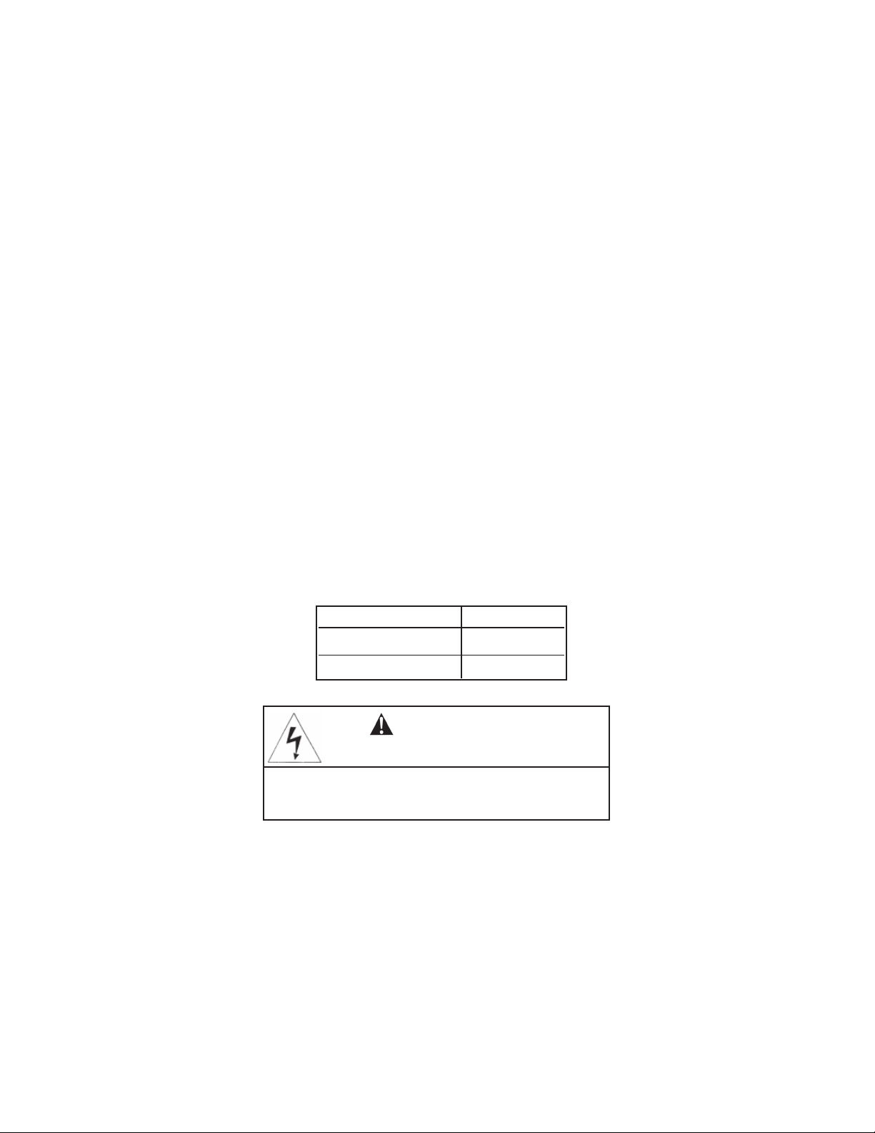
Essential Instructions

READ THIS PAGE BEFORE PROCEEDING!

WARNING

RISK OF ELECTRICAL SHOCK

Your instrument purchase from Emerson is one of the finest available for your particular application. These instruments have been designed, and tested to meet many national and international standards. Experience indicates that its performance is directly related to the quality of the installation and knowledge of the user in operating and maintaining the instrument. To ensure their continued operation to the design specifications, personnel should read this manual thoroughly before proceeding with installation, commissioning, operation, and maintenance of this instrument. If this equipment is used in a manner not specified by the manufacturer, the protection provided by it against hazards may be impaired.

• Failure t o follow th e proper in st ru ct ions may ca use an y one o f the f ollow ing si tuation s to occur: Loss of life; personal injury; property damage; damage to this instrument; and warranty invalidation.

• Ensure that you have received the correct model and options from your purchase order. Verify that this manual covers your model and options. If not, call 1-800-854-8257 or 949-757-8500 to request correct manual.

• For c la rification of i nstructions, con ta ct your Rosemount representative.

• Follow all warnings, cautions, and instructions marked on and supplied with the product.

• Use only qualified personnel to install, operate, update, program and maintain the product.

• Educate your personnel in the proper installation, operation, and maintenance of the product.

• Install equipment as specified in the Installation section of this manual. Follow appropriate local and national codes. Only connect the product to electrical and pressure sources specified in this manual.

• Use only factory documented components for repair. Tampering or unauthorized substitution of parts and procedures can affect the performance and cause unsafe operation of your process.

• All equipment doors must be closed and protective covers must be in place unless qualified personnel are performing maintenance.

Equipment protected throughout by double insulation.

• Installation and servicing of this product may expose personel to dangerous voltages.

• Main power wired to separate power source must be disconnected before servicing.

• Do not operate or energize instrument with case open!

• Signal wiring connected in this box must be rated at least 240 V.

• Non-metallic cable strain reliefs do not provide grounding between conduit connections! Use grounding type bushings and jumper wires.

• Unused cable conduit entries must be securely sealed by non-flammable closures to provide enclosure integrity in compliance with personal safety and environmental protection requirements. Unused conduit openings must be sealed with NEMA 4X or IP65 conduit plugs to maintain the ingress protection rating (NEMA 4X).

• Electrical installation must be in accordance with the National Electrical Code (ANSI/NFPA-70) and/or any other applicable national or local codes.

• Operate only with front panel fastened and in place.

• Safety and performance require that this instrument be connected and properly grounded through a three-wire power source.

• Proper use and configuration is the responsibility of the

user.

CAUTION

This product generates, uses, and can radiate radio frequency energy and thus can cause radio communication interference. Improper installation, or operation, may increase such interference. As temporarily permitted by regulation, this unit has not been tested for compliance within the limits of Class A computing devices, pursuant to Subpart J of Part 15, of FCC Rules, which are designed to provide reasonable protection against such interference. Operation of this equipment in a residential area may cause interference, in which case the user at his own expense, will be required to take whatever measures may be required to correct the interference.

WARNING

Physical access

Unauthorized personnel may potentially cause significant damage to and/or misconfiguration of end users’ equipment. This could be intentional or unintentional and needs to be protected against.

Physical security is an important part of any security program and fundamental to protecting your system. Restrict physical access by unauthorized personnel to protect end users’ assets. This is true for all systems used within the facility.

Page 3

Quick Start Guide

Rosemount 1056 Dual-Input Intelligent Analyzer

1. Refer to Section 2.0 for mechanical installation instructions.

2. Wire sensor(s) to the signal boards. See Section 3.0 for wiring instructions. Refer to the sensor instruction sheet for additional details. Make current output, alarm relay and power connections.

3. Once connections are secured and verified, apply power to the analyzer.

WARNING

RISK OF ELECTRICAL SHOCK

Electrical installation must be in accordance with the National Electrical Code (ANSI/NFPA-70) and/or any other applicable national or local codes.

4. When the analyzer is powered up for the first time, Quick Start screens appear. Quick Start operating tips are as follows:

a. A backlit field shows the position of the cursor.

b. To move the cursor left or right, use the keys to the left or right of the ENTER key. To scroll up or down

or to increase or decrease the value of a digit use the keys above and below the ENTER key . Use the left or right keys to move the decimal point.

c. Press ENTER to store a setting. Press EXIT to leave without storing changes. Pressing EXIT during Quick

Start returns the display to the initial start-up screen (select language).

5. Complete the steps as shown in the Quick Start Guide flow diagram, Fig. A on the following page.

6. After the last step, the main display appears. The outputs are assigned to default values.

7. To change output, and temperature-related settings, go to the main menu and choose Program. Follow the prompts. For a general guide to the Program menu, see the Quick Reference Guide, Fig.B.

8. To return the analyzer to the default settings, choose Reset Analyzer under the Program menu.

Page 4

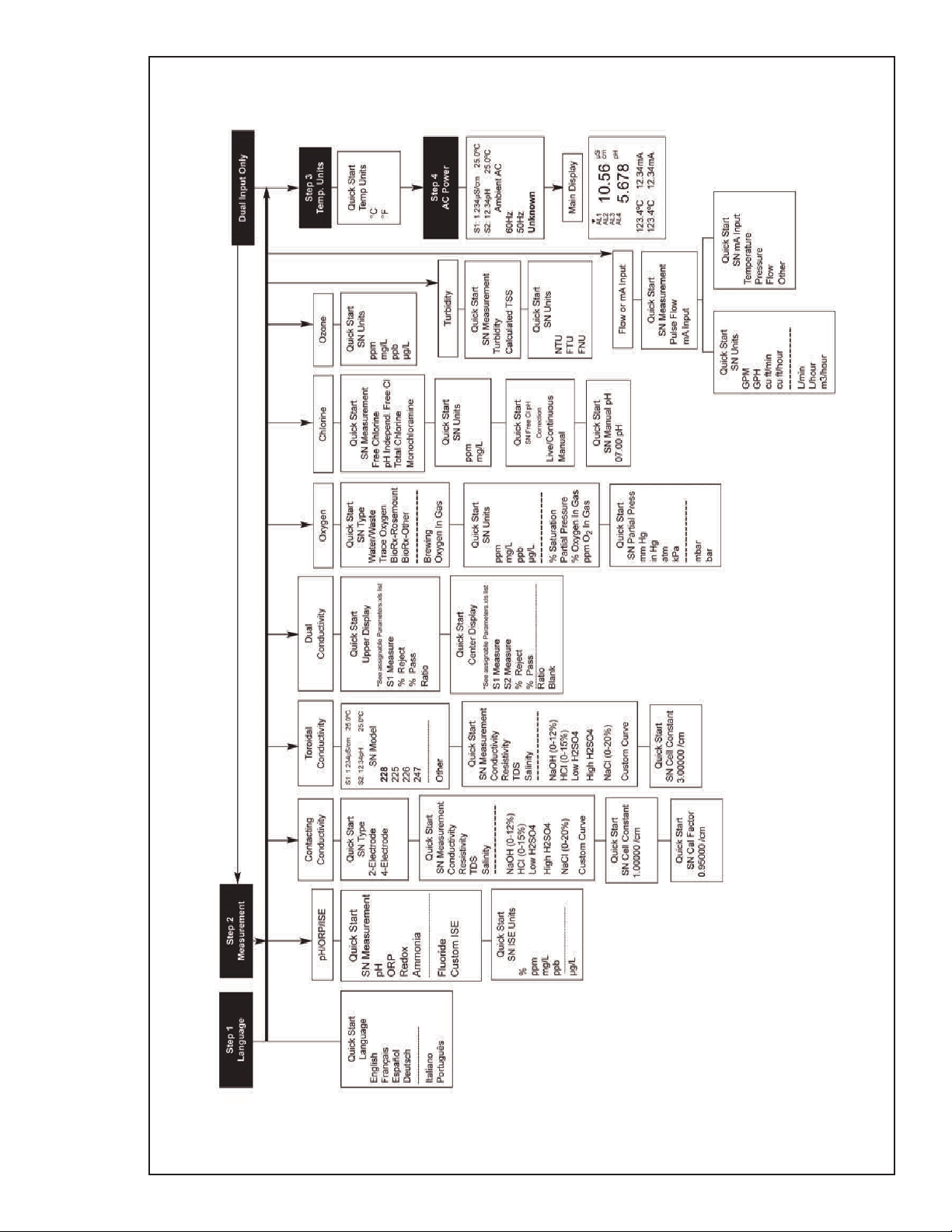
Figure A. Quick Start Guide

Quick Start Guide

Page 5

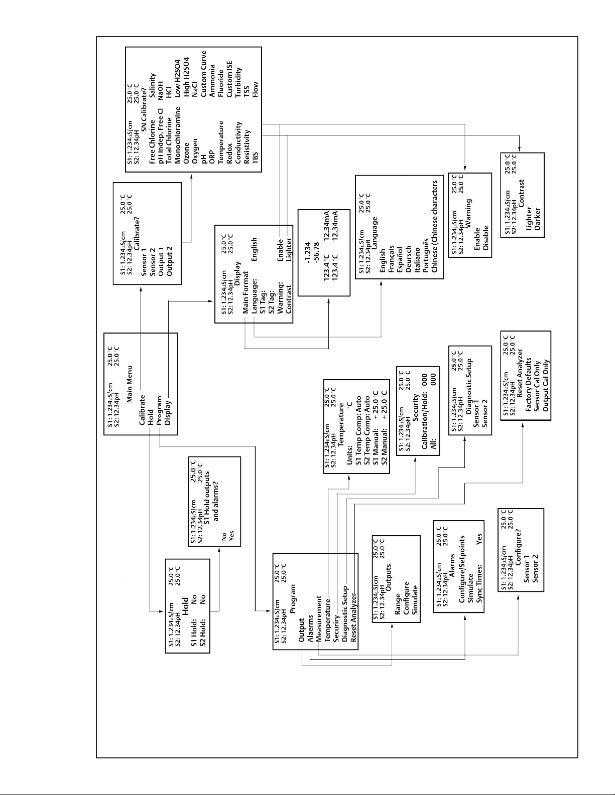
Figure B. Model 1056 Menu Tree

Quick Reference Guide

Page 6

Reference Manual

00809-0100-3156

MODEL 1056

DUAL INPUT INTELLIGENT ANALYZER

TABLE OF CONTENTS

QUICK START GUIDE QUICK REFERENCE GUIDE TABLE OF CONTENTS

Section Title Page

1.0 DESCRIPTION AND SPECIFICATIONS ................................................................ 1

2.0 INSTALLATION ....................................................................................................... 11

2.1 Unpacking and Inspection........................................................................................ 11

2.2 Installation................................................................................................................ 11

3.0 WIRING.................................................................................................................... 21

3.1 General .................................................................................................................... 21

3.2 Preparing Conduit Openings.................................................................................... 21

3.3 Preparing Sensor Cable .......................................................................................... 22

3.4 Power, Output, Alarms and Sensor Connections ..................................................... 22

4.0 DISPLAY AND OPERATION ................................................................................... 29

4.1 User Interface .......................................................................................................... 29

4.2 Instrument Keypad................................................................................................... 29

4.3 Main Display ............................................................................................................ 30

4.4 Menu System ........................................................................................................... 31

5.0 PROGRAMMING – BASICS ................................................................................... 33

5.1 General .................................................................................................................... 33

5.2 Changing the StartUp Settings ................................................................................ 33

5.3 Choosing Temperature units and Automatic/Manual Temperature Compensation .. 34

5.4 Configuring and Ranging the Current Outputs......................................................... 34

5.5 Setting a Security Code ........................................................................................... 36

5.6 Security Access........................................................................................................ 37

5.7 Using Hold ............................................................................................................... 37

5.8 Resetting Factory Defaults – Reset Analyzer .......................................................... 38

5.9 Alarm Relays............................................................................................................ 39

6.0 PROGRAMMING - MEASUREMENTS ................................................................... 43

6.1 Programming Measurements – Introduction ........................................................... 43

6.2 pH ............................................................................................................................ 44

6.3 ORP ......................................................................................................................... 45

6.4 Contacting Conductivity .......................................................................................... 47

6.5 Toroidal Conductivity ................................................................................................ 50

6.6 Chlorine.................................................................................................................... 53

6.6.1 Free Chlorine .................................................................................................. 53

6.6.2 Total Chlorine ................................................................................................. 55

6.6.3 Monochloramine ............................................................................................ 56

6.6.4 pH-independent Free Chlorine ....................................................................... 57

6.7 Oxygen..................................................................................................................... 59

6.8 Ozone ...................................................................................................................... 60

Table of Contents

March 2020

Page 7

Reference Manual

00809-0100-3156

6.9 Turbidity ................................................................................................................... 62

6.10 Flow ......................................................................................................................... 65

6.11 Current Input ............................................................................................................ 66

7.0 CALIBRATION ...................................................................................................... 77

7.1 Calibration – Introduction ......................................................................................... 77

7.2 pH Calibration .......................................................................................................... 78

7.3 ORP Calibration ....................................................................................................... 80

7.4 Contacting Conductivity Calibration ......................................................................... 81

7.5 Toroidal Conductivity Calibration ............................................................................. 84

7.6 Chlorine Calibration ................................................................................................. 86

7.7 Oxygen Calibration .................................................................................................. 94

7.8 Ozone Calibration .................................................................................................... 97

7.9 Temperature Calibration........................................................................................... 99

7.10 Turbidity ................................................................................................................... 100

7.11 Pulse Flow ............................................................................................................... 102

8.0 RETURN OF MATERIAL ........................................................................................ 115

Table of Contents

March 2020

TABLE OF CONTENTS CONT’D

7.6.1 Free Chlorine .................................................................................................. 86

7.6.2 Total Chlorine .................................................................................................. 88

7.6.3 Monochloramine ............................................................................................. 90

7.6.4 pH-Independent Free Chlorine ....................................................................... 92

Warranty................................................................................................................... 115

Page 8

Reference Manual

00809-0100-3156

Section 1.0: Description and Specification

March 2020

Section 1.0

Description and Specifications

• MULTI-PARAMETER INSTRUMENT – single or dual input. Choose from pH/ORP/ISE, Resistivity/Conductivity, % Concentration, Chlorine, Oxygen, Ozone, Temperature, Turbidity, Flow, and 4-20mA Current Input.

• LARGE DISPLAY – large easy-to-read process measurements.

• EASY TO INSTALL – modular boards, removable connectors, easy to wire power, sensors, and outputs.

• INTUITIVE MENU SCREENS with advanced diagnostics and help screens.

• SEVEN LANGUAGES included: English, French, German, Italian, Spanish, Portuguese, and Chinese.

• HART

AND PROFIBUS®DP Digital Communications options

1.1 Features and Applications

The 1056 dual-input analyzer offers single or dual sensor input with an unrestricted choice of dual measurements. This multi-parameter instrument offers a wide range of measurement choices supporting most industrial, commercial, and municipal applications. The modular design allows signal input boards to be field replaced making configuration changes easy. Conveniently, live process values are always displayed during programming and calibration routines.

Quick Start Programming: Exclusive Quick Start screens appear the first time the 1056 is powered. The instrument auto-recognizes each measurement board and prompts the user to configure each sensor loop in a few quick steps for immediate deployment.

Digital Communications: HART and Profibus DP digital communications are available. The 1056 HART units communicate with the Model 375 HART held communicator and HART hosts, such as AMS Intelligent Device Manager. Model 1056 Profibus units are fully compatible with Profibus DP networks and Class 1 or Class 2 masters. HART and Profibus DP configured units will support any single or dual measurement configuration of Model 1056.

hand-

Menus: Menu screens for calibrating and programming are simple and intuitive. Plain language prompts and help screens guide the user through these procedures.

Dual Sensor Input and Output: The 1056 accepts single or dual sensor input. Standar d 0/4-20 mA curr e n t ou t puts c a n be programmed to correspond to any measurement or temperature.

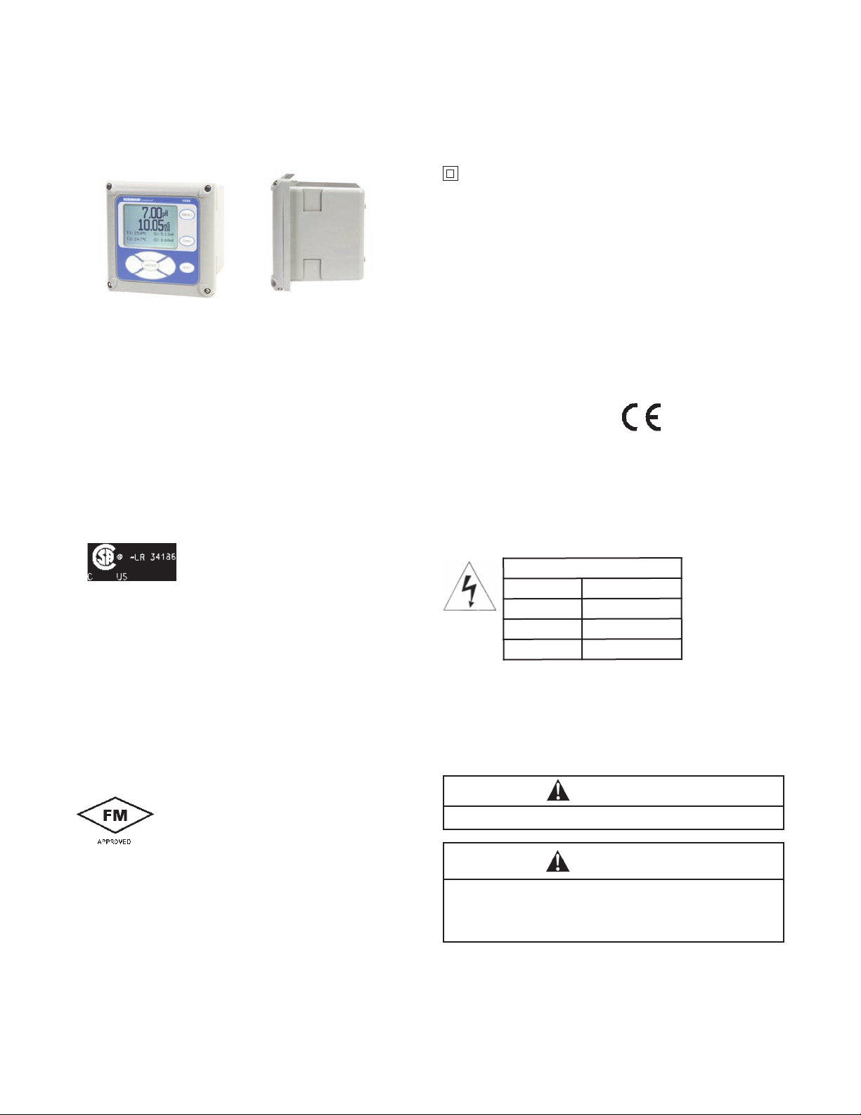
Enclosure: The instrument fits standard ½ DIN panel cutouts. The versatile enclosure design supports panel-mount, pipe-mount, and surface/wall-mount installations.

Isolated Inputs: Inputs are isolated from other signal sources and earth ground. This ensures clean signal inputs for single and dual input configurations. For dual input configurations, isolation allows any combination of measurements and signal inputs without cross-talk or signal interference.

Temperature: Most measurements require temperature compensation. The 1056 will automatically recognize Pt100, Pt1000 or 22k NTC RTDs built into the sensor.

Security Access Codes: Two levels of security access are available. Program one access code for routine calibration and hold of current outputs; program another access code for all menus and functions.

Page 9

Reference Manual

00809-0100-3156

Section 1.0: Description and Specification

March 2020

Diagnostics: The analyzer continuously monitors itself and the sensor(s) for problematic conditions. The display flashes Fault and/or Warning when these conditions occur.

S1: 1.234µS/cm 25.0ºC

S2: 12.34pH 25.0ºC

Diagnostics Faults Warnings Sensor 1 Sensor 2

Out 1: 12.05 mA Out 2: 12.05 mA 1056-01-20-32-HT Instr SW VER: 2.12 AC Freq. Used: 60Hz

Information about each condition is quickly accessible by pressing DIAG on the keypad. User help screens are displayed for most fault and warning conditions to assist in troubleshooting.

Display: The high-contrast LCD provides live measurement readouts in large digits and shows up to four additional process variables or diagnostic parameters. The display is back-lit and the format can be customized to meet user requirements.

LOCAL LANGUAGES:

Rosemount extends its worldwide reach by offering seven local languages – English, French, German, Italian, Spanish, Portuguese, and Chinese. Every unit includes user programming menus; calibration routines; faults and warnings; and user help screens in all seven languages. The displayed language can be easily set and changed using the menus.

Special Measurements: The Model 1056 offers measuring capabilities for many applications.

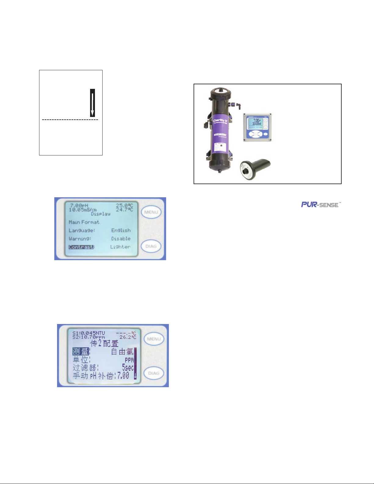
Single or Dual Turbidity: Ideal in municipal applications for measurement of low-NTU filtered drinking water. Must be used with Clarity II sensor, sensor cable and debubbler.

Model T1056

Clarity®II

Turbidimeter

System

4-Electrode Conductivity:

The 1056 is compa tible with Rosem ount 4-electrode Model 410VP in the PUR-SENSE family of conductivity sensors. This sensor supports a wide array of applications and is capable of measuring a large range of conductivity with one geometric configuration. Wired to the 1056, this sensor can measure 2µS/cm to 300mS/cm with an accuracy of 4% of reading throughout the entire range.

4-20mA Current Input: Accepts any analog current input from an external device for temperature compensation of measurements and atmospheric pressure input for partial pressure correction of oxygen.

Selective Ions: The analyzer is able to measure ammonia and fluoride using commercially available ion-selective electrodes. All analyzers with installed pH boards can be programmed to measure selective ions.

Inferential pH: The analyzer is able to derive and display inferred pH (pHCalc) using two contacting conductivity signal boards and the appropriate contacting conductivity sensors. This method will calculate the pH of condensate and boiler water from conductivity and cation conductivity measurements.

Differential Conductivity: Dual input conductivity configurations can measure differential conductivity. The analyzer can be programmed to display dual conductivity as ratio, % rejection, or % passage.

CURRENT OUTPUTS: Two 4-20 mA or 0-20 mA current outputs are electrically isolated. Outputs are fully scalable and can be programmed to linear or logarithmic modes. Output dampening can be enabled with time constants from 0 to 999 seconds. Output 1 includes digital signal 4-20 mA superimposed HART (option -HT only)

Page 10

Reference Manual

00809-0100-3156

Section 1.0: Description and Specification

March 2020

1.2 Specifications - General

Enclosure: Polycarbonate. Type 4X, IP65.

Note: To ensure a water-tight seal, tighten all four front panel

screws to 6 in-lbs of torque

Dimensions: Overall 155 x 155 x 131mm (6.10 x 6.10 x 5.15 in.). Cutout: 1/2 DIN 139mm x 139mm (5.45 x 5.45 in.)

Conduit Openings: Accepts 1/2” or PG13.5 conduit fittings

Display: Monochromatic graphic liquid crystal display.

128 x 96 pixel display resolution. Backlit. Active display area: 58 x 78mm (2.3 x 3.0 in.).

Ambient Temperature and Humidity: 0 to 55 °C

(32 to 131°F). Turbidity only: 0 to 50°C (32 to 122°F), RH 5 to 95% (non-condensing)

Hazardous Location Approvals -

Options for CSA: 01, 02, 03, 20, 21, 22, 24, 25, 26, 27, 30, 31, 32, 34, 35, 36, 37, 38, AN, DP and HT.

Class I, Division 2, Groups A, B, C, & D Class Il, Division 2, Groups E, F, & G

Class Ill T4A Tamb= 50 °C

Type 4X, IP66 Enclosure

Non-Incendive Field Wiring (NIFW) may be used when installed per drawing 1400325. The ‘C’ and ‘US’ indicators adjacent to the CSA Mark signify that the product has been evaluated to the applicable CSA and ANSI/UL Standards, for use in Canada and the U.S. respectively. Evaluated to CSA Standard 22.2 No. 0-10, 0.4-04, 25-1996, 94-M1991, 142-M1987, 213-M1987, 60529-2005/2015. ANSI/IEC 60529-2004/2011. ANSI/ISA 12.12.01:2007. UL No. 50, 11th Ed., 508 17th Ed.

Options for FM: 01, 02, 03, 20, 21, 22, 24, 25, 26, 30, 31, 32, 34, 35, 36, 38, AN, and HT. 01 power supply not available with turbidity sensor options.

Class I, Division 2, Groups A, B, C, & D Class Il & lll, Division 2, Groups E, F, & G T4A -20°C ≤ Tamb ≤ +50°C Enclosure Type 4X

Non-Incendive Field Wiring (NIFW) may be used when installed per drawing 1400324. Evaluated to FM standards 3600:1998, 3611:2004, 3810:2005,ANSI/NEMA 250:2003.

Storage Temperature Effect: -20 to 60 ºC (-4 to 140 °F)

POLLUTION DEGREE 2: Normally only non-conductive

pollution occurs. Occasionally, however, a temporary conductivity caused by condensation must be expected. Altitude: for use up to 2000 meter (6562 ft.)

Power: Code -01: 115/230 VAC ±15%, 50/60 Hz. 10W.

Note: Code -02 and -03 power supplies include four

EMI/RFIEffect

Note 1

During EMI disturbance, the maximum allowable deviation is ±0.004 ppm (4 ppb) for model options 24, 25, 26, 35, 35, and

36.

LVD: EN 61010-1

Alarms relays*: Four alarm relays for process measure-

ment(s) or temperature. Any relay can be configured as a fault alarm instead of a process alarm. Each relay can be configured independently and each can be programmed with interval timer settings.

Relays: Form C, SPDT, epoxy sealed

Inductive load: 1/8 HP motor (max.), 120/240 VAC

*Relays only available with 02 power supply (20 - 30 VDC) or 03 switching power supply (85 - 265 VAC)

Inputs: One or two isolated sensor inputs

Outputs: Two 4-20 mA or 0-20 mA isolated current

Current Output Accuracy: ±0.05 mA @ 25 ºC

Code -02: 20 to 30 VDC. 15 W.

Code -03: 85 to 265 VAC, 47.5 to 65.0 Hz, switching. 15 W.

programmable relays

Equipment protected by double insulation

Meets all industrial requirements of EN 61326.

HART Analog and Digital Communication

No effect on the values being given if using 4-20 mA analog or HART digital signal with shielded, twisted pair wiring.

Profibus DP Digital Communication

No effect on the values being given if using Profibus DP digital signal

Maximum Relay Current

Resistive

28 VDC 115 VAC 230 VAC

5.0 A

CAUTION

RISK OF ELECTRICAL SHOCK

WARNING

Exposure to some chemicals may degrade the sealing properties used in the following devices: Zettler Relays (K1-K4) PN AZ8-1CH-12DSEA

outputs. Fully scalable. Max Load: 550 Ohm.

Output 1 has superimposed HART signal

(1056-0X-2X-3X-HT only)

Page 11

Reference Manual

00809-0100-3156

Section 1.0: Description and Specification

March 2020

Terminal Connections Rating:

Powe r con nector (3-leads): 24-12 AWG wire size. Signal board terminal blocks: 26-16 AWG wire size. Current output connectors (2-leads): 24-16 AWG wire size.

Alarm rela y termi nal b locks: 24- 12 AW G wire si ze (02 24 VDC power supply and -03 85-265VAC power supply)

Weight/Shipping Weight:

(rounded up to nearest lb or nearest 0.5 kg): 3 lbs/4 lbs (1.5 kg/2.0 kg)

Measures conductivity in the

range 0 to 600,000 µS/cm (600mS/cm).

1.3 Contacting Conductivity (Code -20 and -30)

Measurement choices are conductivity, resistivity, total dissolved solids, salinity, and % concentration. The % concentration selection includes the choice of five common solutions (0-12% NaOH, 0-15% HCl, 0-20% NaCl, and 0-25% or 96-99.7% H2SO4).

The conductivity concentration algorithms for these solutions are fully temperature compensated. Three temperature compensation options are available: manual slope (X%/°C), high purity water (dilute sodium chloride), and cation conductivity (dilute hydrochloric acid). Temperature compensation can be disabled, allowing the analyzer to display raw conductivity. For more information concerning the use and operation of the contacting conductivity sensors, refer to the product

data sheets.

Note: When two contacting conductivity sensors are used, Model 1056 can derive an inferred pH value called pHCalc. pHCalc is calculated pH, not directly measured pH.(Model 1056-0X-20-30-AN required)

Note: Selected 4-electrode, high-range contacting conductivity sensors are compatible with Model 1056.

Input filter: time constant 1 - 999 sec, default 2 sec.

Response time: 3 seconds to 100% of final reading

Salinity: uses Practical Salinity Scale

Total Dissolved Solids: Calculated by multiplying

conductivity at 25 ºC by 0.65

Temperature Specifications:

Temperature range 0-150ºC

Temperature Accuracy, Pt-1000, 0-50 ºC

Temperature Accuracy,

Pt-1000, Temp. > 50 ºC

± 0.1ºC

± 0.5ºC

Recommended Sensors For Conductivity

All Rosemount ENDURANCE Model 400 series conductivity sensors (Pt 1000 RTD) and Model 410 sensor.

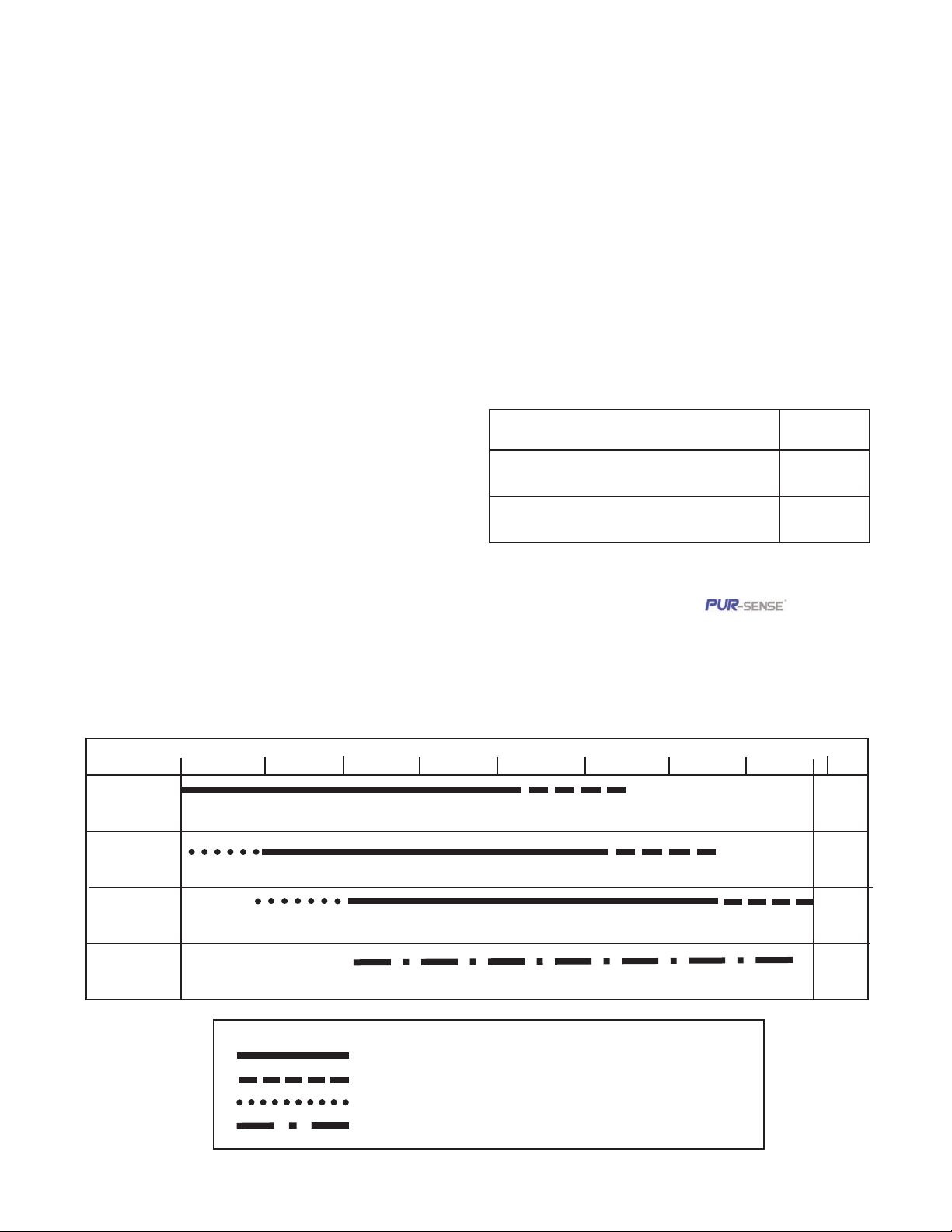
Performance Specifications

Recommended Range – Contacting Conductivity

Cell 0.01µS/cm 0.1µS/cm 1.0µS/cm 10µS/cm 100µS/cm 1000µS/cm 10mS/cm 100mS/cm 1000mS/cm Constant

0.01

0.1

1.0

4-electrode

0.01µS/cm to 200µS/cm

0.1µS/cm to 2000µS/cm

1 µS/cm to 20mS/cm

200µS/cm to 6000µS/cm

2000µS/cm to 60mS/cm

20mS/cm to 600mS/cm

2 µS/cm to 300mS/cm

Cell Constant Linearity

±0.6% of reading in recommended range

+2 to -10% of reading outside high recommended range

±5% of reading outside low recommended range

±4% of reading in recommended range

Page 12

Reference Manual

00809-0100-3156

Section 1.0: Description and Specification

March 2020

1.4 Toroidal Conductivity (Code -21 and -31)

Measures conductivity in the range of 1 (one) µS/cm to 2,000,000 µS/cm (2 S/cm), Measurement choices are conductivity, resistivity, total dissolved solids, salinity, and % concentration. The % concentration selection includes the choice of five common solutions (0-12% Na OH, 0- 15% HCl, 0-20% NaCl, and 0-2 5% or 96-99.7% H2SO4). The conductivity concentration algorithms for these solutions are fully temperature compensated. For other solutions, a simple-to-use menu allows the customer to enter his own data. The analyzer accepts as many as five data points and fits either a linear (two points) or a quadratic function (three or more points) to the data. Two temperature compensation options are available: manual slope (X%/°C) and neutral salt (dilute sodium chloride). Temperature compensation can be disabled, allowing the analyzer to display raw conductivity. Reference temperature and linear temperature slope may also be adjusted for optimum results. For more information concerning the use and operation of the toroidal conductivity sensors, refer to the product data sheets.

Repeatability: ±0.25% ±5 µS/cm after zero cal

Input filter: time constant 1 - 999 sec, default 2 sec.

Response time: 3 seconds to 100% of final reading

Salinity: uses Practical Salinity Scale

Total Dissolved Solids: Calculated by multiplying

conductivity at 25ºC by 0.65

Temperature Specifications:

Temperature range -25 to 210ºC (-13 to 410ºF)

Temperature Accuracy,

Pt-100, -25 to 50 ºC

Temperature Accuracy,

Pt-100,. 50 to 210ºC

± 0.5ºC

± 1ºC

Recommended Sensors

All Rosemount submersion/immersion and flowthrough toroidal sensors.

High performance toroidal conductivity sensors

Models 226 and 225

Performance Specifications

Recommended Range - Toroidal Conductivity

Model 1µS/cm 10µS/cm 100µS/cm 1000µS/cm 10mS/cm 100mS/cm 1000mS/cm 2000mS/cm

226

225 & 228

242

222 (1in & 2in)

5 µS/cm to 500mS/cm

15 µS/cm to 1500mS/cm

100 µS/cm to 2000mS/cm

500 µS/cm to 2000mS/cm

LOOP PERFORMANCE (Following Calibration)

Model 226: ±1% of reading ±5 µS/cm in recommended range Models 225 & 228: ±1% of reading ±10 Models 222,242: ±4% of reading in recommended range

Model 225, 226 & 228: ±5% of reading outside high recommended range

Model 226: ±5 Models 225 & 228: ±15 µS/cm outside low recommended range

µS/cm outside low recommended range

µS/cm in recommended range

500mS/cm to 2000mS/cm

1500mS/cm to 2000mS/cm

Page 13

Reference Manual

00809-0100-3156

1.5 pH/ORP/ISE (Code -22 and -32)

For use with any standard pH or ORP sensor. Measurement choices are pH, ORP, Redox, ammonia, fluoride or custom ISE. The automatic buffer recognition feature uses stored buffer values and their temperature curves for the most common buffer standards available worldwide. The analyzer will recognize the value of the buffer being measured and perform a self stabilization check on the sensor before completing the calibration. Manual or automatic temperature compensation is menu selectable. Change in pH due to process temperature can be compensated using a programmable temperature coefficient. For more information concerning the use and operation of the pH or ORP sensors, refer to the product data sheets.

Model 1056 can also derive an inferred pH value called pHCalc (calculated pH). pHCalc can be derived and displayed when two contacting conductivity sensors are used. (Model 1056-0X-20-30-AN)

Section 1.0: Description and Specification

March 2020

Performance Specifications (ORP Input)

Measurement Range [ORP]: -1500 to +1500 mV

Accuracy: ± 1 mV

Temperature coefficient: ±0.12mV / ºC

Input filter: time constant 1 - 999 seconds, default 4

seconds.

Response time: 5 seconds to 100% of final reading

RECOMMENDED SENSORS FOR pH:

All standard pH sensors.

RECOMMENDED SENSORS FOR ORP:

All standard ORP sensors.

Performance Specifications (pH Input)

Measurement Range [pH]: 0 to 14 pH

Accuracy: ±0.01 pH

Diagnostics: glass impedance, reference impedance

Temperature coefficient: ±0.002pH/ ºC

Solution temperature correction: pure water, dilute

base and custom.

Buffer recognition: NIST, DIN 19266, JIS 8802, BSI,

DIN19267, Ingold, and Merck.

Input filter: time constant 1 - 999 seconds, default 4

seconds.

Response time: 5 seconds to 100%

Temperature Specifications:

Temperature range 0-150 ºC

Temperature Accuracy, Pt-100, 0-50 ºC ± 0.5 ºC

Temperature Accuracy, Temp. > 50 ºC ± 1 ºC

General purpose and high performance pH sensors

Models 396PVP, 399VP and 3300HT

Page 14

Reference Manual

00809-0100-3156

Section 1.0: Description and Specification

March 2020

1.6 Flow (Code -23 and -33)

For use with most pulse signal flow sensors, the 1056 user-selectable units of measurement include flow rates in GPM (Gallons per minute), GPH (Gallon per hour), cu ft/min (cubic feet per min), cu ft/hour (cubic feet per hour), LPM (liters per minute), LPH (liters per hour), or m3/hr (cubic meters per hour), and velocity in ft/sec or m/sec. When configured to measure flow, the unit also acts as a totalizer in the chosen unit (gallons, liters, or cubic meters).

Dual flow instruments can be configured as a % recovery, flow difference, flow ratio, or total (combined) flow.

Performance Specifications

Frequency Range: 3 to 1000 Hz

Flow Rate: 0 - 99,999 GPM, LPM, m3/hr, GPH, LPH,

cu ft/min, cu ft/hr.

1.7 4-20mA Current Input (Code -23 and -33)

For use with any transmitter or external device that transmits 4-20mA or 0-20mA current outputs. Typical uses are for temperature compensation of live measurements (except ORP, turbidity and flow) and for continuous atmospheric pressure input for determination of partial pressure, needed for compensation of live dissolved oxygen measurements. External input of atmospheric pressure for DO measurement allows continuous partial pressure compensation while the Model 1056 enclosure is completely sealed. (The pressure transducer component on the DO board can only be used for calibration when the case is open to atmosphere.)

Externally sourced current input is also useful for calibration of new or existing sensors that require temperature measurement or atmospheric pressure inputs (DO only).

For externally sourced temp or pressure compensation, the user must program the 1056 to input the 4-20mA current signal from the external device.

In addition to live continuous compensation of live measurements, the current input board can also be used simply to display the measured temperature. or the calculated partial pressure from the external device.

Totalized Flow: 0 – 9,999,999,999,999 Gallons or m3, 0 – 999, 999,999,999 cu ft.

Accuracy: 0.5%

Input filter: time constant 0-999 sec., default 5 sec.

Recommended Sensors*

+GF+ Signet 515 Rotor-X Flow sensor

* Input voltage not to exceed ±36V

This feature leverages the large display variables on the Model 1056 as a convenience for technicians. Temperature can be displayed in degrees C or degrees F. Partial pressure can be displayed in inches Hg, mm Hg, atm (atmospheres), kPa (kiloPascals), bar or mbar.

The current input board can be used with devices that do not actively power their 4-20mA output signals. The Model 1056 actively powers to the + and – lines of the current input board to enable current input from a 4-20mA output device.

Note: this Model 1056 signal input board (23, 33 model option code) also includes flow measurement functionality. The signal board, however, must be configured to measure either mA current input or flow.

PERFORMANCE SPECIFICATIONS

Measurement Range *[mA]: 0-20 or 4-20

Accuracy: ±0.03mA

Input filter: time constant 0-999 sec., default 5 sec.

*Current input not to exceed 22mA

Page 15

Reference Manual

00809-0100-3156

Section 1.0: Description and Specification

March 2020

1.8 Chlorine (Code -24 and -34)

Free and Total Chlorine

The 1056 is compatible with the 499ACL-01 free chlorine sensor and the 499ACL-02 total chlorine sensor. The 499ACL-02 sensor must be used with the TCL total chlorine sample conditioning system. The 1056 fully compensates free and total chlorine readings for changes in membrane permeability caused by temperature changes. For free chlorine measurements, both automatic and manual pH correction are available. For automatic pH correction select code 32 and an appropriate pH sensor. For more information concerning the use and operation of the amperometric chlorine sensors and the TCL measurement system, refer to the product data sheets.

Performance Specifications

Resolution: 0.001 ppm or 0.01 ppm – selectable Input Range: 0 nA – 100 µA Automatic pH correction (requires Code P): 6.0 to

10.0 pH

Temperature compensation: Automatic (via RTD) or

manual (0-50°C).

Input filter: time constant 1 - 999 sec, default 5 sec. Response time: 6 seconds to 100% of final reading

Recommended Sensors

Rosemount Model 499ACL-03 Monochloramine sensor

Recommended Sensors*

Chlorine: Model 499ACL-01 Free Chlorine or Model

499ACL-02 Total Residual Chlorine

pH: The following pH sensors are recommended for

automatic pH correction of free chlorine readings: Models: 399-09-62, 399-14, and 399VP-09

Monochloramine

The Model 1056 is compatible with the Model 499A CL-03 Monochloramine sensor. The Model 1056 fully compensates readings for changes in membrane permeability caused by temperature changes. Because monochloramine measurement is not affected by pH of the process, no pH sensor or correction is required. For more information concerning the use and operation of the amperometric chlorine sensors, refer to the product data sheets.

Performance Specifications

Resolution: 0.001 ppm or 0.01 ppm – selectable Input Range: 0nA – 100 Temperature compensation: Automatic (via RTD) or

manual (0-50°C).

Input filter: time constant 1 - 999 sec, default 5 sec. Response time: 6 seconds to 100% of final reading

µA

Page 16

Reference Manual

00809-0100-3156

Section 1.0: Description and Specification

March 2020

1.9 Dissolved Oxygen (Code -25 and -35)

The 1056 is compatible with the 499ADO, 499ATrDO, Hx438, and Gx438 dissolved oxygen sensors and the 4000 percent oxygen gas sensor. The 1056 displays dissolved oxygen in ppm, mg/L, ppb, µg/L, % saturation, % O2in gas, ppm O2in gas. The analyzer fully compensates oxygen readings for changes in membrane permeability caused by temperature changes. An atmospheric pressure sensor is included on all dissolved oxygen signal boards to allow automatic atmospheric pressure determination at the time of calibration. If removing the sensor from the process liquid is impractical, the analyzer can be calibrated against a standard instrument. Calibration can be corrected for process salinity. For more information on the use of amperometric oxygen sensors, refer to the product data sheets.

Performance Specifications

Resolution: 0.01 ppm; 0.1 ppb for 499A TrDO sensor

(when O2<1.00 ppm); 0.1%

Input Range: 0 nA – 100 Temperature Compensation: Automatic (via RTD) or

manual (0-50 °C).

Input filter: time constant 1 - 999 sec, default 5 sec. Response time: 6 seconds to 100% of final reading

µA

1.10 Dissolved Ozone (Code -26 and -36)

The 1056 is compatible with the Model 499AOZ sensor. The 1056 fully compensates ozone readings for changes in membrane permeability caused by temperature changes. For more information concerning the use and operation of the amperometric ozone sensors, refer to the product data sheets.

Performance Specifications

Resolution: 0.001 ppm or 0.01 ppm – selectable Input Range: 0nA – 100 Temperature Compensation: Automatic (via RTD) or

manual (0-35°C)

Input filter: time constant 1 - 999 sec, default 5 sec. Response time: 6 seconds to 100% of final reading

Recommended Sensor

Rosemount Model 499A OZ ozone sensor

µA

Recommended Sensors

Rosemount amperometric membrane and

steam-sterilizable sensors listed above

Dissolved Oxygen sensor with Variopol connection

Model 499ADO

Dissolved Ozone sensors with Polysulfone body

Variopol connection and cable connection

Model 499AOZ

Page 17

Reference Manual

00809-0100-3156

Section 1.0: Description and Specification

March 2020

1.11 Turbidity (Code 27 and 37)

The 1056 instrument is available in single and dual turbidity configurations for the Clarity II®turbidimeter. It is intended for the determination of turbidity in filtered drinking water. The other components of the Clarity II turbidimeter – sensor(s), debubbler/measuring chamber(s), and cable for each sensor must be ordered separately or as a complete system with the Model

1056.

The 1056 turbidity instrument accepts inputs from both USEPA 180.1 and ISO 7027-compliant sensors

When ordering the Model 1056 turbidity instrument, the 02 (24VDC power supply) or the 03 (switching 115/230VAC power supply) are required. Both of these power supplies include four fully programmable relays with timers.

Note: Model 1056 Turbidity must be used with Clarity II sensor, sensor cable and debubbler.

Performance Specifications

Units: Turbidity (NTU, FTU, or FNU); total suspended

solids (mg/L, ppm, or no units)

Display resolution-turbidity: 4 digits; decimal point moves from x.xxx to xxx.

Display resolution-TSS: 4 digits; decimal point moves from x.xxx to xxxx

Calibration methods: user-prepared standard, commercially prepared standard, or grab sample. For total suspended solids user must provide a linear calibration equation.

Inputs: Choice of single or dual input, EPA 180.1 or ISO 7027 sensors.

Field wiring terminals: removable terminal blocks for sensor connection.

Accuracy after calibration at 20.0 NTU:

0-1 NTU ±2% of reading or 0.015 NTU, whichever is greater.

0-20 NTU: ±2% of reading.

Clarity ll Turbidimeter

Page 18

Reference Manual

00809-0100-3156

Section 2.0: Installation

March 2020

Section 2.0 Installation

2.1 Unpacking and Inspection

2.2 Installation

2.1 Unpacking and Inspection

Inspect the shipping container. If it is damaged, contact the shipper immediately for instructions. Save the box. If there is no apparent damage, unpack the container. Be sure all items shown on the packing list are present. If items are missing, notify Emerson immediately.

2.2 Installation

2.2.1 General Information

1. Although the analyzer is suitable for outdoor use, do not install it in direct sunlight or in areas of extreme temperatures.

2. Install the analyzer in an area where vibration and electromagnetic and radio frequency interference are minimized or absent.

3. Keep the analyzer and sensor wiring at least one foot from high voltage conductors. Be sure there is easy access to the analyzer.

4. The analyzer is suitable for panel, pipe, or surface mounting. Refer to the table below.

Type of Mounting Figure

Panel 2-1

Wall and Pipe 2-2

WARNING

RISK OF ELECTRICAL SHOCK

Electrical installation must be in accordance with the National Electrical Code (ANSI/NFPA-70) and/or any other applicable national or local codes.

Page 19

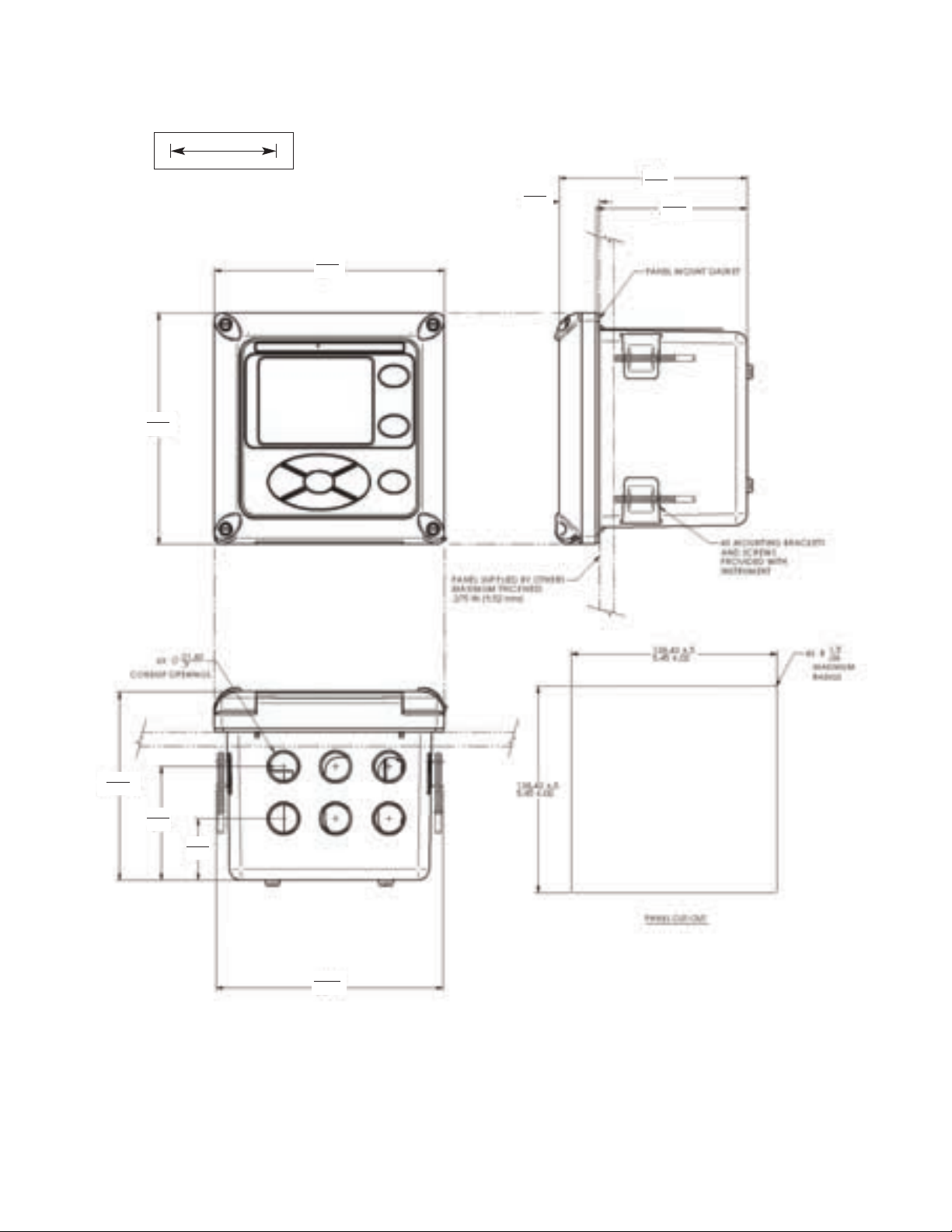
Figure 2-1 Panel Mounting Dimensions

MILLIMETER

INCH

154.9

6.1

154.9

6.1

17.13

1.1

126.4

5.0

101.6

4.00

(

126.4

5.0

Front View

Side View

)

76.2

3.0

41.4

1.6

Bottom View

152.73

6.0

Note: Panel mounting seal integrity (4/4X) for outdoor applications is the responsibility of the end user.

Page 20

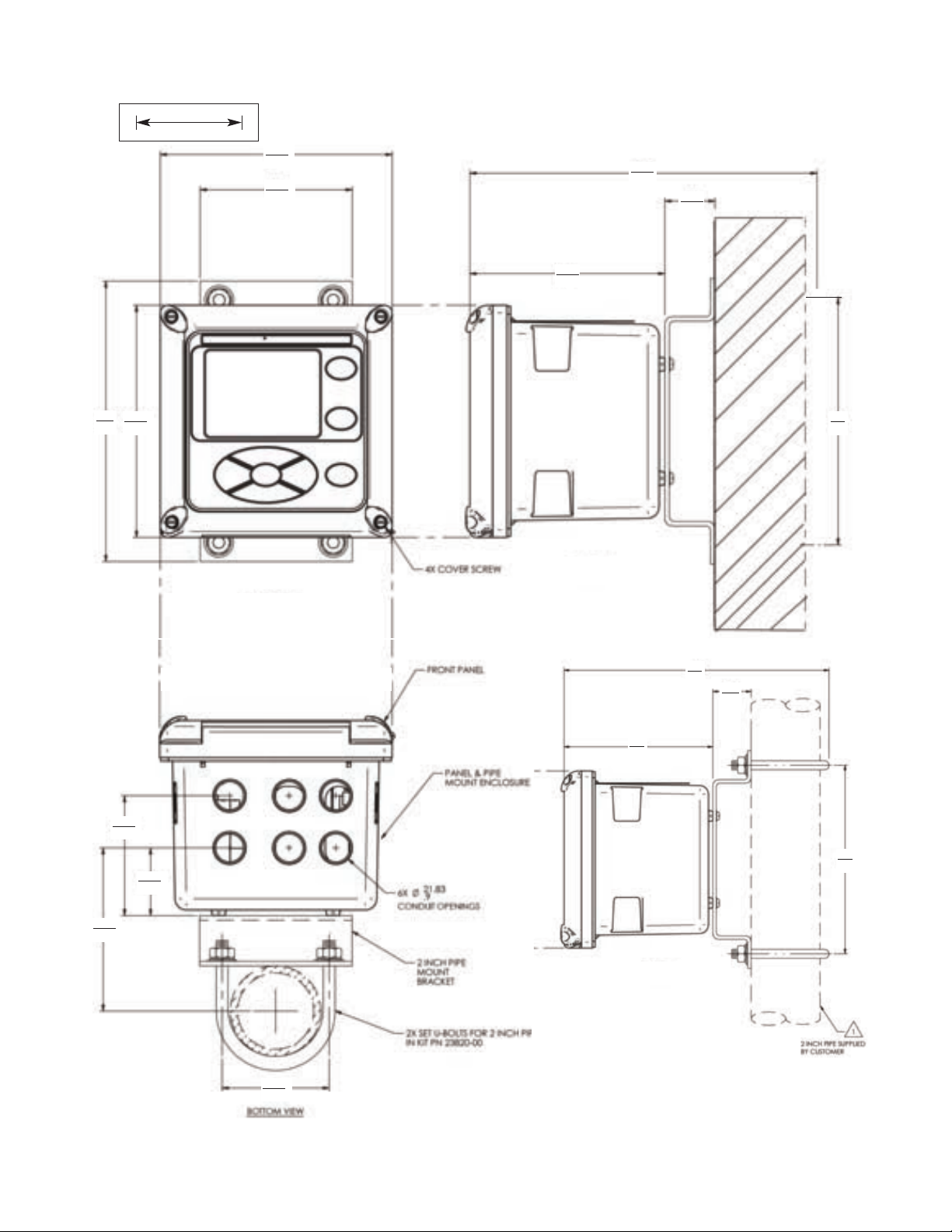
Figure 2-2 Pipe and Wall Mounting Dimensions

(Mounting bracket PN:23820-00)

187

7.4

154.9

6.1

MILLIMETER

INCH

154.9

6.1

102

4.0

Wall / Surface Mount

130

5.1

232

9.1

33.5

1.3

165

6.5

108.9

4.3

80.01

3.2

45.21

1.8

Front View

Bottom View

Pipe Mount

Side View

130

5.1

Side View

232

9.1

33.5

1.3

165

6.5

71.37

2.8

The front panel is hinged at the bottom. The panel swings down for easy access to the wiring locations.

Page 21

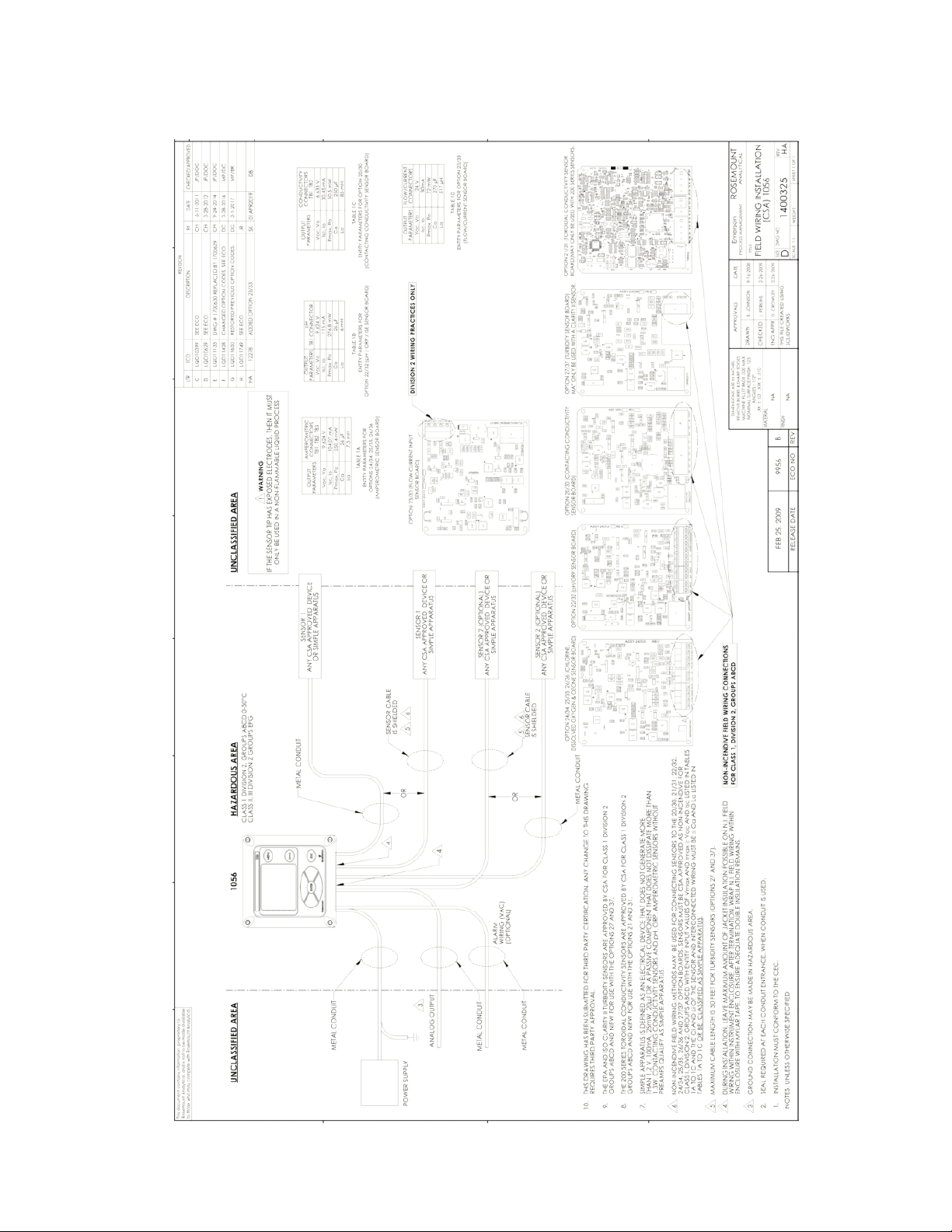
Reference Manual

00809-0100-3156

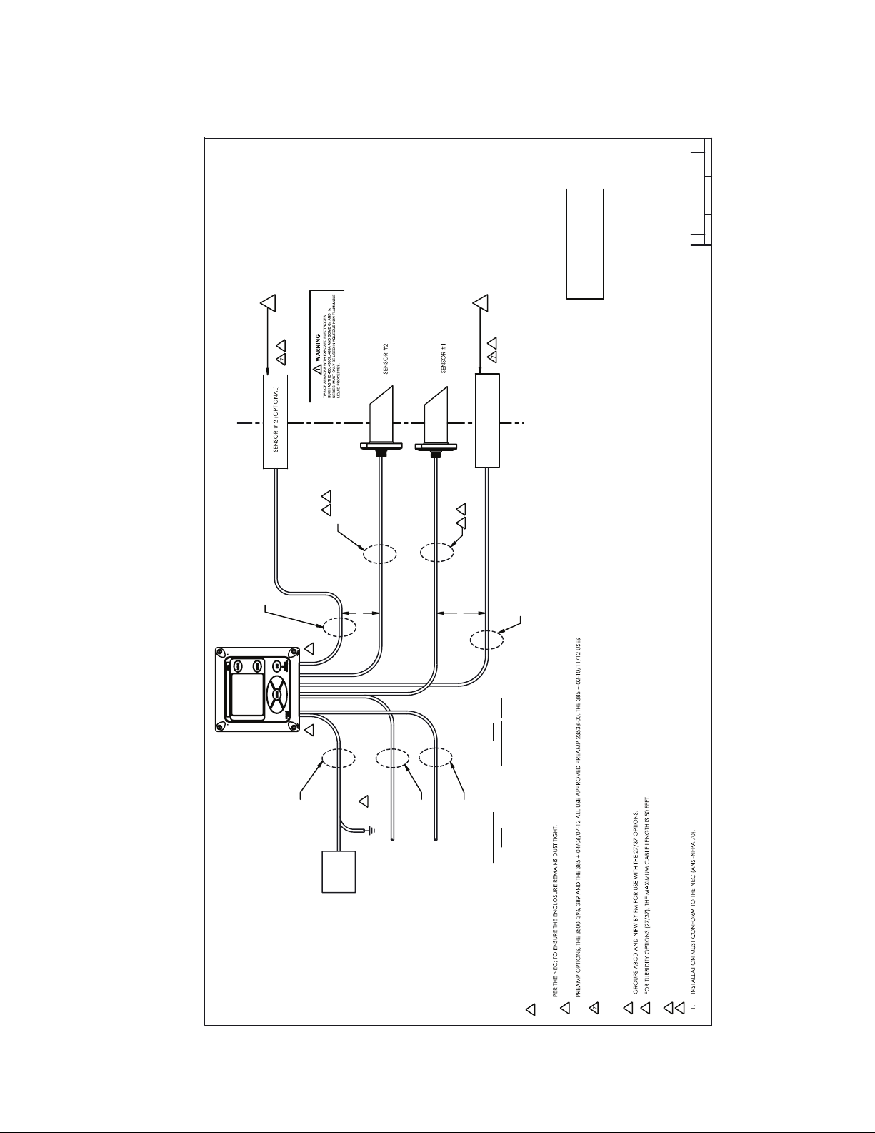
FIGURE 2-3. CSA Non Incendive Field Wiring Installation

Section 2.0: Installation

March 2020

Page 22

Reference Manual

O R

PO W ER SUPPLY

ALARM

W IRING (VAC)

(O PTIO NAL)

AN ALO G O UTPUT

IF A C URRENT LO O P INPUT IS USED W ITH C URREN T/FLO W O PTIO N S (23/33), THE M A XIM U M A LLO W ED VA LUES O F THE INPUTS

ARE: 28 VO LTS, 22mA AN D 616mW AN D THE PO W ER SO URC E M UST BE FM A PPRO VED FO R C LASS 1 DIV ISIO N 2.

9. W H EN INSTALLIN G IN CLASS II AN D III LO C ATIO NS, USE A CLASS II A ND III W IRING M ETHOD

M O DEL 222, 225, 226, 228, 242 A ND 245 TORO IDAL C O NDUC TIVITY SENSORS H AV E BEEN A PPRO VED BY FM FO R USE W ITH THE 1056.

O RP SENSORS W ITH A PPRO VED PREAM PS M A Y BE USED IN 1056 C LASS I D IVISIO N 2 INSTALLA TIO N S. W HEN SELECTED W ITH O RP AN D

A PPRO VED PREAM P 23546-00. O RP SENSO RS W ITHO UT PREAM PS A RE SIM PLE A PPARATUS.

SENSO RS W HICH A RE FM A PPRO VED FO R C LASS I D IVISIO N 2, O R A RE SIM PLE APPA RATUS M A Y BE USED W ITH THE 1056.

SIM PLE APPA RATUS IS DEFINED A S AN ELECTRIC A L DEVICE THAT DO ES N O T G ENERATE M O RE

THAN 1.5V, 100m A , AN D 25 m W O R A PASSIVE C O M PO NENT THAT DO ES N O T D ISSIPA TE

M O RE THAN 1.3W . CONTAC TIN G C O ND UC TIV ITY SENSO RS AND pH SENSO RS W ITHO UT

PREAM PS M A Y BE A SIM PLE APPA RATUS, VERIFY THIS W ITH THE SENSO R M ANUFACTURER.

THE EPA A ND ISO CLARITY II TURBIDITY SENSORS ARE A PPRO VED FO R C LASS 1, D IVISIO N 2

5 4. NO REVISIO N TO DRA W ING W ITHO UT FM APPRO VA L. THIS IS AN A G ENC Y CO NTRO LLED D O C UM EN T.

G RO UN D C O N NEC TIO N M AY BE M A DE IN HAZARDO US AREA.

W H EN C O ND UIT IS USED, A SEAL IS REQUIRED AT EAC H C O NDUIT ENTRAN C E.

M ETAL C O N D UIT

SENSO R CA BLE

IS SHIELDED

SENSO R CA BLE

IS SHIELDED

M ETAL C O N D UIT

SENSO R 1

5 6

C LARITY II

TURBID ITY

(O PTIO NAL)

C LARITY II

TURBID ITY

UNCLASSIFIED

AREA

UNCLASSIFIED

AREA

1056

HAZARDOUS

AREA

C LASS I, DIV. 2, G PS A-D, 0 - 50C

C LASS II, III, D IV 2, G PS E-G

NO TES: UNLESS O THERW ISE SPECIFIED

SCALE: NO NE

W EIG HT:

SIZE

DW G NO

SHEET 1 O F 1

1400324

REV

AG ENC Y C O N TROLLED DRA W ING

AN Y C HAN G E W ILL REQ UIRE

C ERTIFIC A TIO N AG ENC Y

SUBM ITTA L / APPRO VA L

00809-0100-3156

FIGURE 2-3. FM Non Incendive Field Wiring Installation

Section 2.0: Installation

March 2020

Page 23

Reference Manual

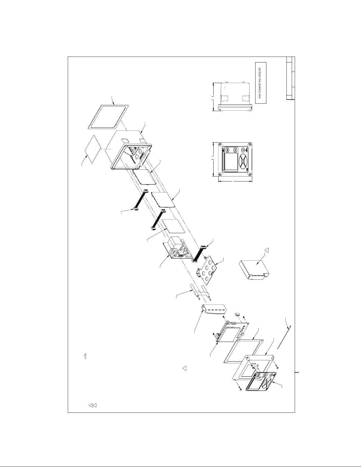
M YLAR AG ENCY

LABEL SEE SHEET 2

2X PO LYCA RBO NATE

10 PIN RIBBO N C ABLE

PO W ER SUPPLY

PCB ASSY

115/230V O R

24VDC O R

85-265VA C

PO LYCA RBO NA TE

TRAN SFORM ER C LAM P

PO LYCA RBO NA TE W IRIN G INSULATOR,

USED W ITH 24VD C PO W ER SUPPLY O PTIO N

W HEN O RDERED W ITH UL O PTIO N

M A IN PCB A SSY

W ITH LCD DISPLAY

NEO PRENE G ASKET

PO LYCA RBO NA TE

ENC LOSURE

SENSOR 1

SIG NA L PC B ASSY

SENSOR 2

SIG NA L PC B ASSY

(O PTIO NAL)

PO LYCA RBO NA TE

14 PIN RIBBO N C ABLE

SS G RO UND ING

PLATE

NEO PRENE G ASKET

PO LYCA RBO NA TE

FRON T CO VER

PO LYESTER OVERLAY

SS HING E W IRE

NO TES: UNLESS O THERW ISE SPECIFIED

1. ALL INSULATING MA TERIALS HA VE C TI

USED W ITH U L O PTIO N O N LY.

INFO RM A TIO N FRO M OTHER AG ENC IES (NO T RATIFIED BY C SA)M AY OPTIO NA LLY APPEAR HERE.

PO LYCA RBO NA TE W IRIN G INSULATOR

USED W ITH 85-265VA C SW ITCH ING PO W ER SUPPLY O PTIO N

W HEN O RDERED W ITH UL O PTIO N

PO LYCA RBO NA TE

PCB IN SULATO R

154.9

6.1

129.1

5.1

NO N-INCEND IVE C LASS 1, D IVISIO N 2 G RO UPS A , B, C & D

T4A Tam b 0-50C

DUST-TIG HT CLASS II D IVISIO N 2, G RO UPS E, F & G

C LASS III ENCLO SURE TYPE 4X

FOR USE IN THE FOLLOW ING

HAZARDOUS (CLASSIFIED) AREAS:

SCALE: 1:2

W EIG HT:

SIZE

DW G NO

SHEET 1 O F 2

1700629

REV

AG ENC Y C O N TROLLED DO C UM ENT

C ERTIFIC A TIO N A G ENC Y

SUBM ITTA L / A PPRO VA L

00809-0100-3156

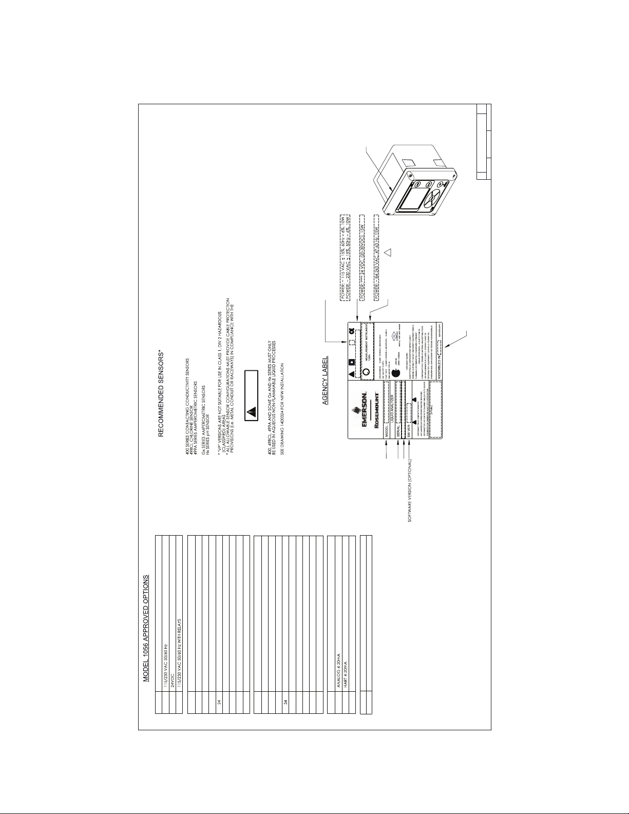
FIGURE 2-3. CSA NonIncendive Class I, Division 2 Certified product for selected configurations

Section 2.0: Installation

March 2020

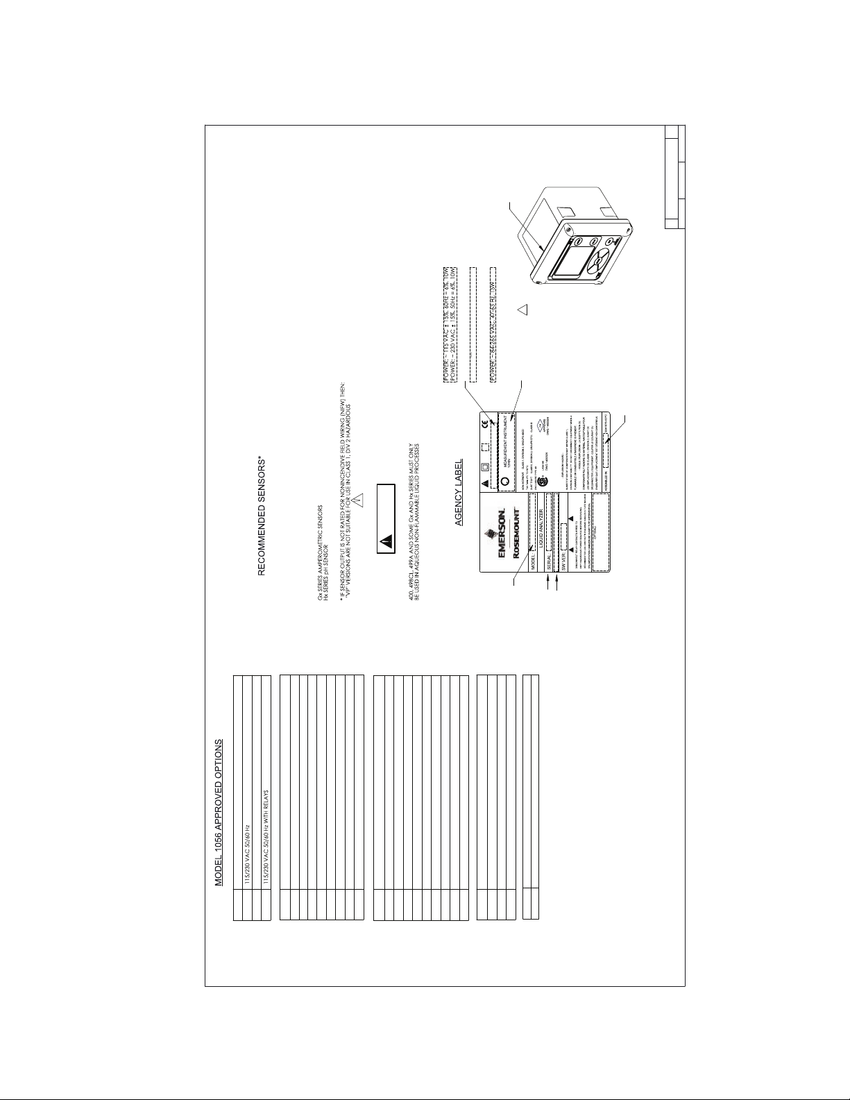
Page 24

Reference Manual

W ARNING

LISTED

AG ENC Y LABEL

TO P EDG E

TIPS O F SENSORS W ITH EXPO SED ELECTRODES SUCH A S THE M O DEL

100 SERIES CONTAC TIN G C O ND UC TIV ITY SENSO RS

200 SERIES TO RO ID AL C O N DUCTIVITY SENSORS

300 SERIES pH SENSO RS

400 SERIES CONTAC TIN G C O ND UC TIV ITY SENSO RS

498CL C HLO RINE SENSO R

499A SERIES AM PERO M ETRIC SENSO RS

3000 SERIES pH SENSO R

SEE DRAW IN G 1400325 FO R N O NINC ENDIV E FIELD W IRIN G (N IFW ) INSTALLATIO N

(C LASSIFIED) AREA S

ALL ALLO W A BLE SENSOR C O NFIG URATIO NS M UST PRO VIDE CA BLE PRO TECTIO N

PROVISIO N S (i.e. M ETAL CO ND UIT O R RAC EW A YS) IN C O M PLIAN C E W ITH THE

CA NAD IAN ELEC TRIC A L CO DE

M O D EL O PTIO N C O DE EXAM PLES:

1056-02-24-38-HT-UL

1056-03-22-38-HT

M O D EL O PTIO N STRING

SERIA L N UM BER

ASSEMBLY LOCA TIO N

IF O PTIO N UL, PRINT THIS

IF O PTIO N 01, PRINT:

ELSE, IF O PTIO N 02 PRIN T:

PO W ER: --- 24 VDC , (20-30VDC ), 15W

ELSE, IF O PTIO N 03 PRIN T:

BAR CODE

W ARNING

WARNING

AVERTISSEMENT

ORDINARY LOCATION:

HAZARDOUS LOCATION:

DESIG N AUTHO RITY LOC A TIO N

C O DE

PO W ER SUPPLY

24VDC

C O DE

M EASUREMENT 2 30 C O NTAC TIN G CO ND UC TIVITY31 TORO IDA L CO ND UC TIV ITY32 pH/O RP/ISE34 C HLO RINE35 DISSO LVED O XYG EN36 O ZONE37 TURBID ITY (W HEN IN STALLED PER DRA W ING 1400325)33 FLO W /CU RRENT INPUT38 NONE

C O DE

O UTPUTSAN ANA LOG 4-20m AHT HA RT 4-20m ADP PRO FIBUS DP PRO TOC O L

C O DE

M EASUREMENT 1 20 C O NTAC TIN G CO ND UC TIVITY21 TORO IDA L CO ND UC TIV ITY22 pH/O RP/ISE24 C HLO RINE25 DISSO LVED O XYG EN26 O ZONE27 TURBID ITY (W HEN IN STALLED PER DRA W ING 1400325)23 FLO W /CU RRENT INPUT

C O DE

UL APPROVAL (BLA NK IF NO NE SELECTED)UL UL O RD INA RY LO C ATIO NS A PPRO VAL

REV

1700629

SHEET 2 O F 2

DW G NO

SIZE

W EIG HT:

SCALE: 1:2

NO TES: UNLESS O THERW ISE SPECIFIED

00809-0100-3156

FIGURE 2-3. CSA NonIncendive Class I, Division 2 Certified product for selected configurations

Section 2.0: Installation

March 2020

Page 25

Reference Manual

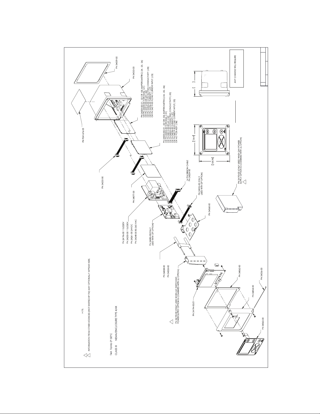
M YLAR

AG ENC Y LABEL

SEE SHEET 2

2X PO LYCA RBO NATE

10 PIN RIBBO N

C ABLE

PO W ER SUPPLY ASSY

O R

PO LYCA RBO NA TE

TRAN SFORM ER C LAM P

O R

PO LYCA RBO NA TE W IRIN G INSULATOR

M A IN PCB A SSY

W ITH LC D DISPLA Y

NEO PRENE G ASKET

PO LYCA RBO NA TE

ENC LOSURE

SENSOR 1

SIG NA L PC B ASSY

SENSOR 2

SIG NA L PC B ASSY

PO LYCA RBO NA TE

SS G RO UND ING

PLATE

NEO PRENE G ASKET

PO LYCA RBO NA TE

FRON T CO VER

PO LYESTER O VERLAY

SS HING E W IRE

NO TES: UNLESS O THERW ISE SPECIFIED

1. ALL INSULATIN G M ATERIALS HAVE C TI

USED W ITH UL O PTIO N O NLY.

PO LYCA RBO NA TE W IRIN G INSULATOR

PO LYCA RBO NA TE

PCB IN SULATOR

O VERA LL DIM ENSIO N S

PRO FIBUS BO ARD

RIBBO N C ABLE

SEE SHEET 2

6.1

129.1

5.1

NO N-INC END IVE C LASS 1, D IVISIO N 2 G RO UPS A, B, C & D

DUST-TIG HT C LASS II D IVISIO N 2, G RO UPS E, F & G

FOR USE IN THE FOLLOW ING

HAZARDOUS (CLASSIFIED) AREAS:

SCALE: 1:2

W EIG HT:

SIZE

DW G NO

SHEET 1 O F 2

1700630

REV

AG ENC Y C O N TROLLED DO C UM ENT

C ERTIFIC A TIO N AG ENC Y

SUBM ITTA L/ APPRO V AL

00809-0100-3156

Section 2.0: Installation

March 2020

FIGURE 2-3. FM NonIncendive Class I, Division 2 Certified product for selected configurations

Page 26

Reference Manual

W ARNING

LISTED

AG ENC Y LABEL

TO P EDG E

TIPS O F SENSORS W ITH EXPO SED ELECTRODES SUCH A S THE M O D EL

100 SERIES C O NTAC TIN G CO ND UC TIVITY SENSORS

200 SERIES TO RO ID AL C O N DU CTIVITY SENSORS

300 SERIES p H SENSO RS

3000 SERIES pH SENSO R

IF NO NINC END IVE FEILD W IRING M ETHO D S ARE NO T USED, THEN:

NA TIO N AL ELECTRIC AL C O D E

1056 O PTIO N C O DE EXAM PLES:

1056PP03ANKC

1056CL02HTN5

M O D EL O PTIO N STRING

SERIA L NUM BER

ASSEMBLY LOCA TIO N

PRINTED IF O PTIO N UL

IF O PTIO N 01, PRINT:

ELSE, IF O PTIO N 02 PRIN T:

ELSE, IF O PTIO N 03 PRIN T:

BAR CODE

W ARNING

WARNING

AVERTISSEMENT

ORDINARY LOCATION:

HAZARDOUS LOCATION :

C HIN A RoHS LO G O M AY BE PRINTED H ERE

DESIG N AUTHORITY A DD RESS

CODE

POW ER SUPPLY

010203

CODE

MEASUREMENT 2

C O NTAC TIN G CO ND UC TIVITY31 TORO IDAL C O NDUC TIVITY32 pH/O RP/ISE

C HLO RINE35 DISSO LVED O XYG EN36 O ZO NE37 TURBID ITY33 FLO W /CURRENT INPUT38 NO NE

CODE

OUTPUTS

PRO FIBUS DP PRO TOC O L

CODE

M EASUREMENT 1

C O NTAC TIN G CO ND UC TIVITY21 TORO IDAL C O NDUC TIVITY22 pH/O RP/ISE

C HLO RINE25 DISSO LVED O XYG EN36 O ZO NE27 TURBID ITY23 FLO W /CURRENT INPUT

CODE

UL APPROVAL (BLANK IF NONE SELECTED)

UL O RD INARY LO C ATIO NS A PPRO VAL

REV

1700630

SHEET 2 O F 2

DW G NO

SIZE

W EIG HT:

SCALE: 1:2

NO TES: UNLESS O THERW ISE SPECIFIED

00809-0100-3156

FIGURE 2-3. FM NonIncendive Class I, Division 2 Certified product for selected configurations

Section 2.0: Installation

March 2020

Page 27

Reference Manual

00809-0100-3156

Section 2.0: Installation

March 2020

Page 28

Reference Manual

00809-0100-3156

Section 3.0: Wiring

March 2020

Section 3.0

Wiring

3.1 General

3.2 Preparing Conduit Openings

3.3 Preparing Sensor Cable

3.4 Power, Output, and Sensor Connections

3.1 General

The 1056 is easy to wire. It includes removable connectors and slide-out signal input boards. The front panel is hinged at the bottom. The panel swings down for easy access to the wiring locations.

3.1.1. Removable connectors and signal input boards

Model 1056 uses removable signal input boards and communication boards for ease of wiring and installation. Each of the signal input boards can be partially or completely removed from the enclosure for wiring. The Model 1056 has three slots for placement of up to two signal input boards and one communication

board.

Slot 1-Left Slot 2 – Center Slot 3 – Right

Comm. board Input Board 1 Input Board 2

3.1.2 Signal Input Boards

Slots 2 and 3 are for signal input measurement boards. Wire the sensor leads to the measurement board following the lead locations marked on the board. After wiring the sensor leads to the signal board, carefully slide the wired board fully into the enclosure slot and take up the excess sensor cable through the cable gland. Tighten the cable gland nut to secure the cable and ensure a sealed enclosure.

3.1.3 Digital Communication Boards

HART and Profibus DP communication boards will be available in the future as options for Model 1056 digital communication with a host. The HART board supports Bell 202 digital communications over an analog 4-20mA current output. Profibus DP is an open communications protocol which operates over a dedicated digital line to the host.

3.1.4 Alarm Relays

Four alarm relays are supplied with the switching power supply (85 to 265VAC, 03 order code) and the 24VDC power supply (20-30VDC, 02 order code). All relays can be used for process measurement(s) or temperature. Any relay can be configured as a fault alarm instead of a process alarm. Each relay can be configured independently and each can be programmed as an interval timer, typically used to activate pumps or control valves. As process alarms, alarm logic (high or low activation or USP*) and deadband are user-programmable. Customer-defined failsafe operation is supported as a programmable menu function to allow all relays to be energized or not-energized as a default condition upon powering the analyzer. The USP* alarm can be programmed to activate when the conductivity is within a user-selectable percentage of the limit. USP alarming is available only when a contacting conductivity measurement board is installed.

3.2 Preparing Conduit Openings

There are six conduit openings in all configurations of Model 1056. (Note that four of the openings will be fitted with plugs upon shipment.)

Conduit openings accept 1/2-inch conduit fittings or PG13.5 cable glands. To keep the case watertight, block unused openings with NEMA 4X or IP65 conduit plugs.

NOTE: Use watertight fittings and hubs that comply with your requirements. Connect the conduit hub to the conduit before attaching the fitting to the analyzer.

Page 29

Reference Manual

00809-0100-3156

Section 3.0: Wiring

March 2020

3.3 Preparing Sensor Cable

The 1056 is intended for use with all Rosemount sensors. Refer to the sensor installation instructions for details on preparing sensor cables.

3.4 Power, Output, and Sensor Connections

3.4.1 Power Wiring

Three Power Supplies are offered for Model 1056:

a. 115/230 VAC Power Supply (-01 ordering code)

b. 24 VDC (20 – 30V) Power Supply (-02 ordering code)

c. 85 – 265 VAC Switching Power Supply (-03 ordering code)

AC mains (115 or 230 V) leads and 24 VDC leads are wired to the Power Supply board which is mounted vertically on the left side of the main enclosure cavity. Each lead location is clearly marked on the Power Supply board. Wire the power leads to the Power Supply board using the lead markings on the board.

The grounding plate is connected to the earth terminal of power supply input connector TB1 on the -01 (115/230 VAC) and -03 (85-265 VAC) power supplies. The green colored screws on the grounding plate are intended for connection to some sensors to minimize radio frequency interference. The green screws are not intended to be used for safety purposes.

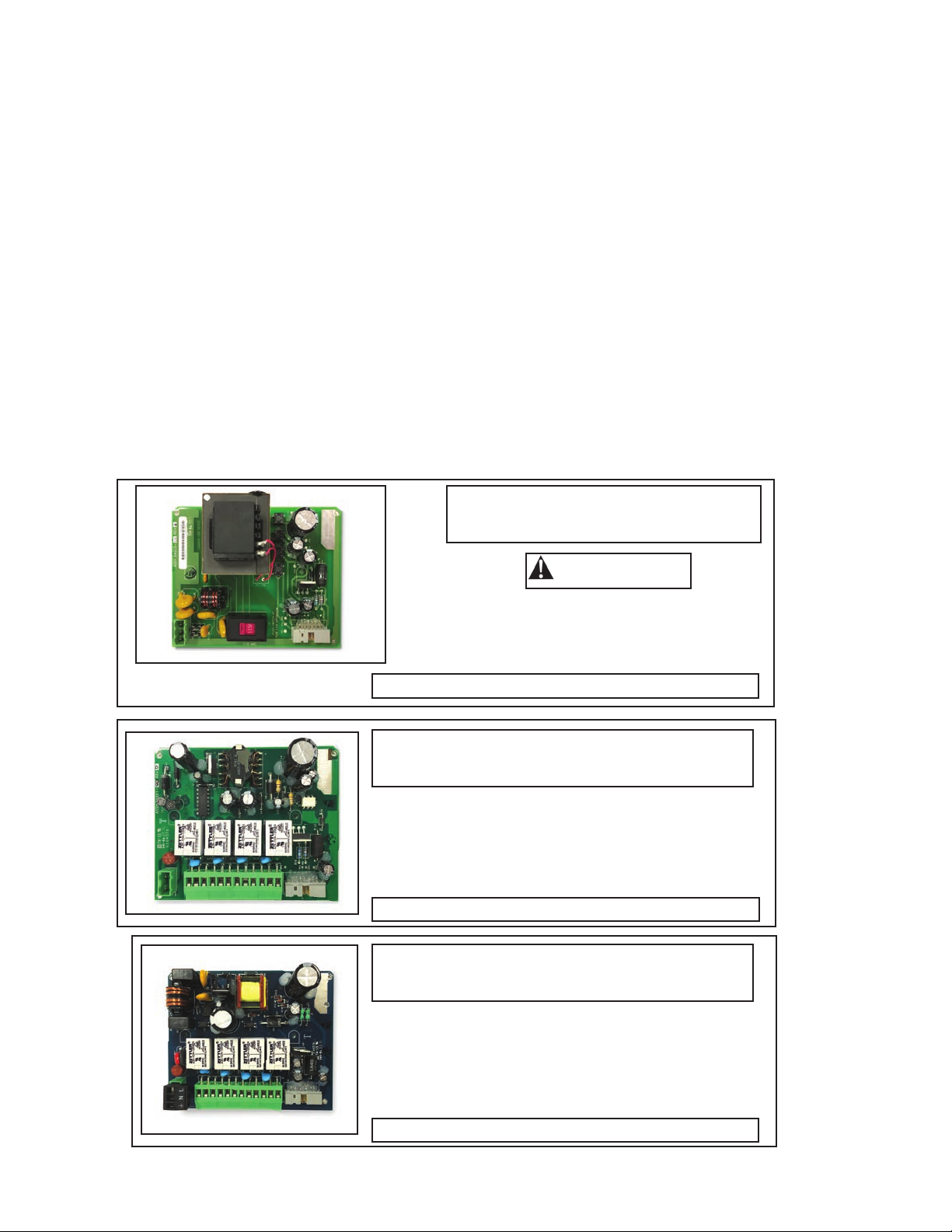
115/230 VAC Power Supply (-01 ordering code) is shown below:

CAUTION

AC Power switch shipped in the 230 VAC position. Adjust switch upwards to 115 VAC position

for 110 VAC – 120 VAC operation.

Figure 3-1

24 VDC Power Supply (-02 ordering code) is shown below:

This power supply automatically detects DC power and accepts 20 VDC to 30 VDC inputs.

Four programmable alarm relays are included.

Figure 3-2

Switching AC Power Supply (-03 ordering code) is shown below:

This power supply automatically detects AC line conditions and switches to the proper line voltage and line frequency.

Four programmable alarm relays are included.

Figure 3-3

Page 30

Reference Manual

00809-0100-3156

Section 3.0: Wiring

March 2020

3.4.2 Current Output Wiring

All instruments are shipped with two 4-20 mA current outputs. Wiring locations for the outputs are on the Main board which is mounted on the hinged door of the instrument. Wire the output leads to the correct position on the Main board using the lead markings (+/positive,

-/negative) on the board. Male mating connectors are provided with each unit.

Note

Twisted pairs are required to minimize noise pickup in

Figure 3-4 4-20 mA current outputs. For high EMI/RFI environments, shielded sensor wire is required and recommended in all other installations.

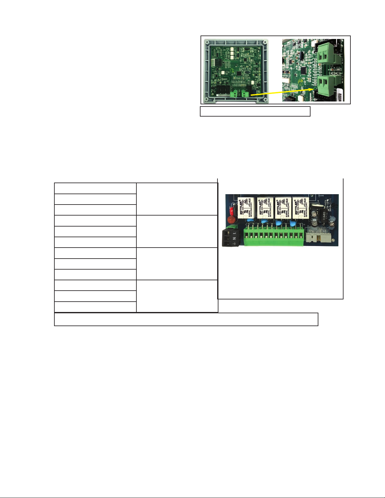
3.4.3 Alarm Relay Wiring

Four alarm relays are supplied with the switching power supply (85 to 265VAC, -03 order code) and the 24VDC power supply (20-30 VDC, -02 order code). Wire the relay leads on each of the independent relays to the correct position on the power supply board using the printed lead markings (NO/Normally Open, NC/Normally Closed, or Com/Common) on the board. See Fig 3-4.

NO1

RELAY 1COM1

NC1

NO2

RELAY 2COM2

NC2

NO3

RELAY 3COM3

NC3

NO4

RELAY 4COM4

NC4

Figure 3-5 Alarm Relay Wiring for Model 1056 Switching Power Supply (-03 Order Code)

3.4.4 Sensor Wiring to Signal Boards

Wire the correct sensor leads to the measurement board using the lead locations marked directly on the b o a r d . After wiring the sensor leads to the signal board, carefully slide the wired board fully into the enclosure slot and take up the excess sensor cable through the cable gland.

For best EMI/RFI protection use shielded output signal cable enclosed in an earth-grounded metal conduit. Connect the shield to earth ground. AC wiring should be 14 gauge or greater. Provide a switch or breaker to disconnect the analyzer from the main power supply. Install the switch or breaker near the analyzer and label it as the disconnecting device for the analyzer.

Keep sensor and output signal wiring separate from power wiring. Do not run sensor and power wiring in the sameconduit or close together in a cable tray.

NOTE:

Twisted pairs are required to minimize noise pickup in the flow and current sensor inputs. For high EMI/RFI environments, shielded sensor wire is required and recommended in all other installations.

Page 31

Reference Manual

00809-0100-3156

Section 3.0: Wiring

March 2020

WARNING

RISK OF ELECTRICAL SHOCK

Electrical installation must be in accordance with the National Electrical Code (ANSI/NFPA-70) and/or any other applicable national or local codes.

Figure 3-6 Contacting Conductivity signal board and Sensor cable leads

Figure 3-7 Toroidal Conductivity Signal board and Sensor cable leads

Page 32

Reference Manual

00809-0100-3156

Section 3.0: Wiring

March 2020

Figure 3-8 pH/ORP/ISE signal board and Sensor cable leads

Figure 3-9 Amperometric signal (Chlorine, Oxygen, Ozone) board and Sensor cable leads

Page 33

Reference Manual

00809-0100-3156

Section 3.0: Wiring

March 2020

Figure 3-10 Turbidity signal board with plug-in Sensor connection

Figure 3-11 Flow/Current Input signal board and Sensor cable leads

Page 34

Reference Manual

00809-0100-3156

Section 3.0: Wiring

March 2020

FIGURE 3-12 Power Wiring for the 1056 115/230VAC Power Supply (-01 Order Code)

FIGURE 3-13 Power Wiring for the 1056 85-265 VAC Power Supply (-03 ordering code)

Page 35

Reference Manual

00809-0100-3156

Section 3.0: Wiring

March 2020

FIGURE 3-14 Output Wiring for Model 1056 Main PCB

To Main PCB

FIGURE 3-15 Power Wiring for Model 1056 24VDC Power Supply (-02 ordering code)

Page 36

Reference Manual

00809-0100-3156

Section 4.0

Display and Operation

4.1 User Interface

4.2 Keypad

4.3 Main Display

4.4 Menu System

4.1 User Interface

The 1056 has a large display which shows two live measurement readouts in large digits and up to four additional process variables or diagnostic parameters concurrently. The display is back-lit and the format can be customized to meet user requirements. The intuitive menu system allows access to Calibration, Hold (of current outputs), Programming, and Display functions by pressing the MENU button. In addition, a dedicated DIAGNOSTIC button is available to provide access to useful operational information on installed sensor(s) and any problematic conditions that might occur. The display flashes Fault and/or Warning when these conditions occur. Help screens are displayed for most fault and warning conditions to guide the user in troubleshooting. During calibration and programming, key presses cause different displays to appear. The displays are selfexplanatory and guide the user step-by-step through the procedure.

Section 4.0: Display and Operation

March 2020

4.2 Instrument Keypad

There are 4 Function keys and 4 Selection keys on the instrument keypad.

Function keys:

The MENU key is used to access menus for programming and calibrating the instrument. Four top-level menu items appear when pressing the MENU key:

 Calibrate: calibrate attached sensors and

analog outputs.

 Hold: Suspend current outputs.  Program: Program outputs, measurement,

temperature, security and reset.

 Display: Program display format, language,

warnings, and contrast Pressing MENU always causes the main menu screen to appear. Pressing MENU followed by EXIT causes

the main display to appear.

Page 37

Reference Manual

00809-0100-3156

Section 4.0: Display and Operation

March 2020

Pressing the DIAG key displays active Faults and Warnings, and provides detailed instrument information and sensor diagnostics including: Faults, Warnings, Sensor 1 and 2 information, Out 1 and Out 2 live current values, Instrument Software version, and AC frequency used. Pressing ENTER on Sensor 1 or Sensor 2 provides useful diagnostics and information (as applicable): Measurement, Sensor Type, Raw signal value, Cell constant, Zero Offset, Temperature, Temperature Offset, selected measurement range,

Selection keys:

Surrounding the ENTER key, four Selection keys – up, down, right and left, move the cursor to all areas of the screen while using the menus. Selection keys are used to:

1. select items on the menu screens

2. scroll up and down the menu lists.

3. enter or edit numeric values.

4. move the cursor to the right or left

5. select measurement units during operations

4.3 Main Display

The Model 1056 displays one or two primary measurement values, up to four secondary measurement values, a fault and warning banner, alarm relay flags, and a digital communications icon.

Cable Resistance, Temperature Sensor Resistance, Signal Board software version.

The ENTER key. Pressing ENTER stores numbers and settings and moves the display to the next screen.

The EXIT key. Pressing EXIT returns to the previous screen without storing changes.

Process measurements:

Two process variables are displayed if two signal boards are installed. One process variable and process temperature is displayed if one signal board is installed with one sensor. The Upper display area shows the Sensor 1 process reading. The Center display area shows the Sensor 2 process reading. For dual conductivity, the Upper and Center display areas can be assigned to different process variables as follows:

Process variables for Upper display- example: Process variables for Center display- example:

Measure 1 Measure 1

% Reject Measure 2

% Pass % Reject

Ratio % Pass

Ratio

Blank

For single input configurations, the Upper display area shows the live process variable and the Center display area can be assigned to Temperature or blank.

Slope 1 Man Temp 2

Displayable Secondary Values

Ref Off 1 Output 1 mA

Secondary values:

Up to four secondary values are shown in four display quadrants at the bottom half of the screen. All four secondary value positions can be programmed by the user to any display parameter available. Possible secondary values include:

Gl Imp 1 Output 2 mA

Ref Imp 1 Output 1 %

Raw Output 2 %

mV Input Measure 1

Temp 1 Blank

Man Temp 1

Page 38

Reference Manual

00809-0100-3156

Section 4.0: Display and Operation

March 2020

Fault and Wa rning banner:

If the analyzer detects a problem with itself or the sensor the word Fault or Warning will appear at the bottom of the display. A fault requires immediate attention. A warning indicates a problematic condition or an impending failure. For troubleshooting assitance, press Diag.

For matt ing the Main D ispl ay

The main display screen can be programmed to show primary process variables, secondary process variables and diagnostics.

1. Press MENU

2. Scroll down to Display. Press ENTER.

3. Main Format will be highlighted. Press ENTER.

4. The sensor 1 process value will be highlighted in reverse video. Press the selection keys to navigate down to the screen sections that you wish to program. Press ENTER.

5. Choose the desired display parameter or diagnostic for each of the four display sections in the lower screen.

6. Continue to navigate and program all desired screen sections. Press MENU and EXIT. The screen will return to the main display.

For single sensor configurations, the default display shows the live process measurement in the upper display area and temperature in the center display area. The user can elect to disable the display of temperature in the center display area using the Main Format function. See Fig. 4-1 to guide you through programming the main display to select process parameters and diagnostics of your choice.

For dual sensor configurations, the default display shows Sensor 1 live process measurement in the upper display area and Sensor 2 live process measurement temperature in the center display area. See Fig. 4-1 to guide you through programming the main display to select process parameters and diagnostics of your choice.

4.4 Menu System

Model 1056 uses a scroll and select menu system. Pressing the MENU key at any time opens the top-level menu including Calibrate, Hold, Program and Display functions.

To find a menu item, scroll with the up and down keys until the item is highlighted. Continue to scroll and select menu items until the desired function is chosen. To select the item, press ENTER. To return to a previous menu level or to enable the main live display, press the EXIT key repeatedly. To return immediately to the main display from any menu level, simply press MENU then EXIT.

The selection keys have the following functions:  The Up key (above ENTER) increments numerical values, moves the decimal place one place to the right,

or selects units of measurement.

 The Down key (below ENTER) decrements numerical values, moves the decimal place one place to the

left, or selects units of measurement

 The Left key (left of ENTER) moves the cursor to the left.  The Right key (right of ENTER) moves the cursor to the right.

To access desired menu functions, use the “Quick Reference” Figure B. During all menu displays (except main display format and Quick Start), the live process measurements and secondary measurement values are displayed in the top two lines of the Upper display area. This conveniently allows display of the live values during important calibration and programming operations.

Menu screens will time out after two minutes and return to the main live display.

Page 39

Reference Manual

00809-0100-3156

Section 5.0: Programming the Analyzer - Basics

March 2020

FIGURE 4-1 Formatting the Main Display

Page 40

Reference Manual

00809-0100-3156

Section 5.0: Programming the Analyzer - Basics

Section 5.0

Programming The Analyzer - Basics

5.1 General

5.2 Changing Start-Up Settings

5.3 Programming Temperature

5.4 Configuring and Ranging 4-20ma Outputs

5.5 Setting Security Codes

5.6 Security Access

5.7 Using Hold

5.8 Resetting Factory Defaults – Reset Analyzer

5.9 Programming Alarm Relays

5.1 General

Section 5.0 describes the following programming functions:

 Changing the measurement type, measurement units and temperature units.  Choose temperature units and manual or automatic temperature compensation mode  Configure and assign values to the current outputs  Set a security code for two levels of security access  Accessing menu functions using a security code  Enabling and disabling Hold mode for current outputs  Choosing the frequency of the AC power (needed for optimum noise rejection)  Resetting all factory defaults, calibration data only, or current output settings only

March 2020

5.2 Changing Startup Settings

5.2.1 Purpose

To change the measurement type, measurement units, or temperature units that were initially entered in Quick Start, choose the Reset analyzer function (Sec. 5.9) or access the Program menus for sensor 1 or sensor 2 (Sec.

6.0). The following choices for specific measurement type, measurement units are available for each sensor measurement board.

TABLE 5-1. Measurements and Measurement Units

Signal board Available measurements

pH/ORP (22, 32)

Contacting conductivity (20, 30)

Toroidal conductivity

(21, 31)

Chlorine (24, 34)

Oxygen (25, 35)

Ozone (-26, -36) Ozone

Temperature (all)

pH, ORP, Redox, Ammonia, Fluoride, Custom ISE

Conductivity, Resistivity, TDS, Salinity, NaOH (0-12%), HCl (0-15%), Low H2SO4, High H2SO4, NaCl (0-20%), Custom Curve

Free Chlorine, pH Independ. Free Cl, Total Chlorine, Monochloramine

Oxygen (ppm), Trace Oxygen (ppb), Percent Oxygen in gas, Salinity

Temperature °C. ºF

5.2.2 Procedure

Follow the Reset Analyzer procedure (Sec 5.8) to reconfigure the analyzer to display new measurements or measurement units. To change the specific measurement or measurement units for each signal board type, refer to the Program menu for the appropriate measurement (Sec. 6.0).

Measurements units:

pH, mV (ORP) %, ppm, mg/L, ppb,

µg/L, (ISE)

µS/cm, mS/cm, S/cm

% (concentration)

µS/cm, mS/cm, S/cm

% (concentration)

ppm, mg/L

ppm, mg/L, ppb, µg/L % Sat, Partial Pressure, % Oxygen In Gas, ppm Oxygen In Gas

ppm, mg/L, ppb, µg/L

Page 41

Reference Manual

00809-0100-3156

Section 5.0: Programming the Analyzer - Basics

March 2020

5.3 Choosing Temperature Units And Automatic/Manual Temperature Compensation

5.3.1 Purpose

Most liquid analytical measurements (except ORP) require temperature compensation. The Model 1056 performs temperature compensation automatically by applying internal temperature correction algorithms. Temperature correction can also be turned off. If temperature correction is off, the Model 1056 uses the temperature entered by the user in all temperature correction calculations.

5.3.2 Procedure

Follow the menu screens in Fig. 5.1 to select automatic or manual temp compensatio n, set the manual reference temperature, and to program temperature units as °C or °F.

Figure 5-1. Choosing Temp Units and Manual Auto Temp Compensation

S1: 1.234µS/cm 25.0ºC

S2: 12.34pH 25.0ºC

Temperature Units: °C S1 Temp Comp: Auto S2 Temp Comp: Auto S1 Manual: +25.0°C

S2 Manual: +25.0ºC

5.4 Configuring and Ranging The Current Outputs

5.4.1 Purpose

The Model 1056 accepts inputs from two sensors and has two analog current outputs. Ranging the outputs means assigning values to the low (0 or 4 mA) and high (20 mA) outputs. This section provides a guide for configuring and ranging the outputs. ALWAYS CONFIGURE THE OUTPUTS FIRST.

5.4.2 Definitions

1. CURRENT OUTPUTS. The analyzer provides a continuous output current (4-20 mA or 0-20 mA) directly proportional to the process variable or temperature.

The low and high current outputs can be set to any value.

2. ASSIGNING OUTPUTS. Assign a measurement to Output 1 or Output 2.

3. DAMPEN. Output dampening smooths out noisy readings. It also increases the response time of the output. Output dampening does not affect the response time of the display.

4. MODE. The current output can be made directly proportional to the displayed value (linear mode) or directly proportional to the common logarithm of the displayed value (log mode).

Page 42

Reference Manual

00809-0100-3156

Section 5.0: Programming the Analyzer - Basics

March 2020

5.4.3 Procedure: Configure Outputs

Under the Program/Outputs menu, the adjacent screen will appear to allow configuration of the outputs. Follow the menu screens in Fig. 5-2 to configure the outputs.

5.4.4 Procedure: Assigning Measurements the Low and High Current Outputs

The adjacent screen will appear when entering the Assign function under Program/Output/Configure. These screens allow you to assign a measurement, process value, or temperature input to each output. Follow the menu screens in Fig. 5-2 to assign measurements to the outputs.

5.4.5 Procedure: Ranging the Current Outputs

The adjacent screen will appear under Program/Output/Range. Enter a value for 4mA and 20mA (or 0mA and 20mA) for each output. Follow the menu screens in Fig. 5-2 to assign values to the outputs.

S1: 1.234µS/cm 25.0ºC

S2: 12.34pH 25.0ºC

OutputM Configure

Assign: S1 Meas Range: 4-20mA Scale: Linear Dampening: 0sec

Fault Mode: Fixed Fault Value: 21.00mA

S1: 1.234µS/cm 25.0ºC

S2: 12.34pH 25.0ºC

OutputM Assign

S1 Measurement S1 Temperature S2 Measurement S2 Temperature

S1: 1.234µS/cm 25.0ºC

S2: 12.34pH 25.0ºC

Output Range OM SN 4mA: 0.000µS/cm OM SN 20mA: 20.00µS/cm OM SN 4mA: 00.00pH OM SN 20mA: 14.00pH

Figure 5-2. Configuring and Ranging the Current Outputs

Page 43

Reference Manual

00809-0100-3156

Section 5.0: Programming the Analyzer - Basics

March 2020

5.5 Setting A Security Code

5.5.1 Purpose

The security codes prevent accidental or unwanted changes to program settings, displays, and calibration. Model 1056 has two levels of security code to control access and use of the instrument to different types of users. The two levels of security are:

- All: This is the Supervisory security level. It allows access to all menu functions, including

Programming, Calibration, Hold and Display.

- Calibration/Hold: This is the operator or

technician level menu. It allows access to

only calibration and Hold of the current outputs.

5.5.2 Procedure

1. Press MENU. The main menu screen appears.

Choose Program.

Figure 5-3. Setting a Security Code

S1: 1.234µS/cm 25.0ºC S2: 12.34pH 25.0ºC

Program

Outputs

MAIN MENU

Program

Measurement Temperature

Security

Diagnostic Setup Ambient AC Power:Unk

Reset Analyzer

2. Scroll down to Security. Select Security.

3. The security entry screen appears. Enter a three digit security code for each of the desired security levels. The security code takes effect

two minutes after the last key stroke. Record the security code(s) for future access and communication to operators or technicians as needed.

4. The display returns to the security menu screen. Press EXIT to return to the previous screen. To return to t he ma in displ ay, press ME NU followed by EXIT.

Fig. 5-3 displays the security code screens.

S1: 1.234µS/cm 25.0ºC S2: 12.34pH 25.0ºC

Security

Calibration/Hold: 000

All: 000

Page 44

Reference Manual

00809-0100-3156

Section 5.0: Programming the Analyzer - Basics

March 2020

5.6 Security Access

5.6.1 How the Security Code Works

When entering the correct access code for the Calibration/Hold security level, the Calibration and Hold menus are accessible. This allows operators or technicians to perform routine maintenance. This security level does not allow access to the Program or Display menus. When entering the correct access code for All security level, the user has access to all menu functions, including Programming, Calibration, Hold and Display.

5.6.2 Procedure

1. If a security code has been programmed, selecting the Calibrate, Hold, Program or Display top menu items causes the security access screen to appear

2. Enter the three-digit security code for the appropriate security level.

S1: 1.234µS/cm 25.0ºC

S2: 12.34pH 25.0ºC

Security Code

000

3. If the entry is correct, the appropriate menu screen appears. If the entry is incorrect, the Invalid Code screen appears. The Enter Security Code screen reappears after 2 seconds.

5.7 UsingHold

5.7.1 Purpose

The analyzer output is always proportional to measured value. To prevent improper operation of systems or pumps that are controlled directly by the current output, place the analyzer in hold before removing the sensor for calibration and maintenance. Be sure to remove the analyzer from hold once calibration is complete. During hold, both outputs remain at the last value. Once in hold, all current outputs remain on

Hold indefinitely.

5.7.2 Using the Hold Function

To hold the outputs,

1. Press MENU. The main menu screen appears. Choose Hold.

2. The Hold Outputs and Alarms? screen appears. Choose Yes to place the analyzer in hold. Choose No to take the analyzer out of hold. Note: There are no alarm relays with this con figuration. Current outputs are included with all configurations.

3. The Hold screen will then appear and Hold

wi ll remain on i ndefinitely unt il H old is disabled.

See figure 5-1 below.

MAIN MENU

Figure 5-4. Using Hold

S1: 1.234µS/cm 25.0ºC S2: 12.34pH 25.0ºC

Hold

S1 Hold: No S2 Hold: No

Hold

S1: 1.234µS/cm 25.0ºC

S2: 12.34pH 25.0ºC

S1 Hold outputs

and alarms? No Yes

Page 45

Reference Manual

00809-0100-3156

Section 5.0: Programming the Analyzer - Basics

March 2020

5.8 Resetting Factory Default Settings

5.8.1 Purpose

This section describes how to restore factory calibration and default values. The process also clears all fault messages and returns the display to the first Quick Start screen. The Model 1056 offers three options for resetting factory defaults.

a. reset all settings to factory defaults b. reset sensor calibration data only c. reset analog output settings only

5.8.2. Procedure

To reset to factory defaults, reset calibration data only or reset analog outputs only, follow the Reset Analyzer flow diagram.

Figure 5-5. Resetting Factory Default Settings

Page 46

Reference Manual

00809-0100-3156

Section 5.0: Programming the Analyzer - Basics

March 2020

5.9 Programming Alarm Relays

5.9.1 Purpose

The Model 1056 24VDC (02 order code) and the AC switching power supply (03 order code) provide four alarm relays for process measurement or temperature. Each alarm can be configured as a fault alarm instead of a process alarm. Also, each relay can be programmed independently and each can be programmed as an interval timer. This section describes how to configure alarm relays, simulate relay activation, and synchronize timers for the four alarm relays. This section provides details to program the following alarm features:

Sec.

5.9.2

5.9.3

5.9.4 Set relay logic High Program relay to activate at High or Low reading

5.9.5 Deadband: 0.00uS/cm

5.9.6 USP Safety: 0%↓ Program percentage of the limit to activate the alarm

5.9.7

5.9.8 Interval time: 24.0 hr Time in hours between relay activations

5.9.9

5.9.10

5.9.11

5.9.12 Simulate

5.9.13

Under the Program/Alarms menu, this screen will appear to allow configuration of the alarm relays. Follow the menu screens in Fig. XX to configure the outputs.

Alarm relay feature: default Description

Enter Setpoint 100.0uS/cm Enter alarm trigger value

Assign measurement S1 Measure Select alarm assignment

Program the change in process value after the relay deactivates

Normal state: Open

On-Time: 10 min Enter the time in seconds that the relay is activated.

Recover time: 60 sec Enter time after the relay deactivation for process recovery

Hold while active: S1 Holds current outputs during relay activation

Synchronize Timers Yes Control the timing of two or more relay timers set as Interval timers

Program relay default condition as open or closed for failsafe operation

Manually simulate alarms to confirm relay operation

S1: 1.234µS/cm 25.0ºC

S2: 12.34pH 25.0ºC

Alarms Configure/Setpoint Simulate Synchronize Timers: Yes

This screen will appear to allow selection of a specific alarm relay. Select the desired alarm and press ENTER.

This screen will appear next to allow complete programming of each alarm. Factory defaults are displayed as they would appear for an installed contacting conductivity board. USP Safety only appears if alarm logic is set to “USP”. Interval timer, On Time, Recover Time, and Hold While Active only appear if the alarm is configured as an Interval timer.

S1: 1.234µS/cm 25.0ºC

S2: 12.34pH 25.0ºC

Configure/Setpoint Alarm 1 Alarm 2 Alarm 3 Alarm 4

S1: 1.234µS/cm 25.0ºC

S2: 12.34pH 25.0ºC

AlarmM Settings

Setpoint: 100.0uS/cm Assign: S1 Measure Logic: High Deadband: 0.00uS/cm USP Safety: 0%↓

Interval time: 24.0 hr On Time: 120 sec Recover time: 60 sec Hold while active: Sens1

Page 47

Reference Manual

00809-0100-3156

Section 5.0: Programming the Analyzer - Basics

March 2020

5.9.2 Procedure – Enter Setpoints

Under the Program/Alarms menu, this screen will appear to allow configuration of the alarm relays. Enter the desired value for the process measurement or temperature at which to activate an alarm event.

5.9.3 Procedure – Assign Measurement

Under the Alarms Settings menu, this screen will appear to allow assignment of the alarm relays. select an alarm assignment. Additional assignment choices are shown in Figure X-X depending on which measurement board(s) is installed.

5.9.4 Procedure – Set Relay Logic

Under the Alarms Settings menu, this screen will appear to set the alarm logic. Select the desired relay logic to activate alarms at a High reading or a Low reading. USP Safety only appears if a contacting conductivity board is installed.

S1: 1.234µS/cm 25.0ºC

S2: 12.34pH 25.0ºC

Alarm1 S2 Setpoint

+100.0uS/cm

S1: 1.234µS/cm 25.0ºC

S2: 12.34pH 25.0ºC

AlarmM Assign:

S1 Measurement S1 Temperature S2 Measurement S2 Temperature Interval Timer Fault Off

S1: 1.234µS/cm 25.0ºC

S2: 12.34pH 25.0ºC

AlarmM Logic:

High Low USP

5.9.5 Procedure – Deadband

Under the Alarms Settings menu, this screen will appear to program the deadband as a measurement value. Enter the change in the process value needed after the relay deactivates to return to normal (and thereby preventing repeated alarm activation).

5.9.6 Procedure – USP Safety

Under the Alarms Settings menu, this screen will appear to program the USP alarm setting. Enter the percentage below the limit at which to activate the alarm.

5.9.7 Procedure – Normal State

The user can define failsafe condition in software by programming the alarm default state to normally open or normally closed upon power up. To display this alarm configuration item, enter the Expert menus by holding down the EXIT key for 6 seconds while in the main display mode. Select Yes upon seeing the screen prompt: “Enable Expert Menu?” Under the Alarms Settings menu, this screen will appear to set the normal state of the alarms. Select the alarm condition that is desired each time the analyzer is powering up.

S1: 1.234µS/cm 25.0ºC

S2: 12.34pH 25.0ºC

Alarm1 Deadband

+000.5uS/cm

S1: 1.234µS/cm 25.0ºC

S2: 12.34pH 25.0ºC

Alarm1 USP Safety

+0%

S1: 1.234µS/cm 25.0ºC

S2: 12.34pH 25.0ºC

Alarm2 Normal State

Open

Closed

Page 48

Reference Manual

00809-0100-3156

Section 5.0: Programming the Analyzer - Basics

March 2020

5.9.8 Procedure – Interval time

Under the Alarms Settings menu, this screen will appear to set the interval time. Enter the fixed time in hours between relay activations.

5.9.9 Procedure – On time

Under the Alarms Settings menu, this screen will appear to set the relay on time. Enter the time in seconds that the relay is activated.

5.9.10 Procedure – Recovery time

Under the Alarms Settings menu, this screen will appear to set the relay recovery time. Enter time after the relay deactivation for process recovery.

5.9.11 Procedure – Hold while active

Under the Alarms Settings menu, this screen will appear to program the feature that Holds the current outputs while alarms are active. Select to hold the current outputs for Sensor 1, Sensor 2 or both sensors while the relay is activated.

S1: 1.234µS/cm 25.0ºC

S2: 12.34pH 25.0ºC

Alarm1 Interval Time

024.0 hrs

S1: 1.234µS/cm 25.0ºC

S2: 12.34pH 25.0ºC

Alarm1 On-Time

00.00sec

S1: 1.234µS/cm 25.0ºC

S2: 12.34pH 25.0ºC

Alarm1 Recovery

060sec

S1: 1.234µS/cm 25.0ºC

S2: 12.34pH 25.0ºC

Alarm1 Hold while active Sensor 1 Sensor 2 Both None

5.9.12 Procedure – Simulate

Alarm relays can be manually set for the purposes of checking devices such as valves or pumps. Under the Alarms Settings menu, this screen will appear to allow manual forced activation of the alarm relays. Select the desired alarm condition to simulate.

5.9.13 Procedure – Synchronize

Under the Alarms Settings menu, this screen will appear to allow Synchronization of alarms that are set to interval timers. Select yes or no to Synchronize two or more timers.

S1: 1.234µS/cm 25.0ºC

S2: 12.34pH 25.0ºC

Simulate Alarm M

Don’t simulate De-energize Energize

S1: 1.234µS/cm 25.0ºC

S2: 12.34pH 25.0ºC

Synchronize Timers

Yes

Page 49

Reference Manual

00809-0100-3156

Section 6.0: Programming the Measurements

March 2020

Page 50

Reference Manual

00809-0100-3156

6.1 Configuring Measurements – Introduction

6.2 pH

6.3 ORP

6.4 Contacting Conductivity

6.5 Toroidal Conductivity

6.6 Chlorine

6.6.1 Free Chlorine

6.6.2 Total Chlorine

6.6.3 Monochloramine

6.6.4 pH-Independent Free Chlorine

6.7 Oxygen

6.8 Ozone

Section 6.0: Programming the Measurements

March 2020

Section 6.0

Programming - Measurements

6.9 Turbidity

6.10 Flow

6.11 Current Input

6.1 Programming Measurements – Introduction

The Model 1056 automatically recognizes each installed measurement board upon first power-up and each time the analyzer is powered. Completion of Quick Start screens upon first power up enable measurements, but additional steps may be required to program the analyzer for the desired measurement application. This section covers the following programming and configuration functions;

1. Selecting measurement type or sensor type (all sections)

2. Identifying the preamp location (pH-see Sec. 6.2)

3. Enabling manual temperature correction and entering a reference temperature (all sections)

4. Enabling sample temperature correction and entering temperature correction slope (selected sections)

5. Defining measurement display resolution (pH and amperometric)

6. Defining measurement display units (all sections)

7. Adjusting the input filter to control display and output reading variability or noise (all sections)

8. Selecting a measurement range (conductivity – see Sec’s 6.4, 6.5)

9. Entering a cell constant for a contacting or toroidal sensor (see Sec’s 6.4, 6.5)

10. Entering a temperature element/RTD offset or temperature slope (conductivity-see Sec’s 6.4)

11. Creating an application-specific concentration curve (conductivity-see Sec’s 6.4, 6.5)

12. Enabling automatic pH correction for free chlorine measurement (Sec. 6.6.1)

To fully configure the analyzer for each installed measurement board, you may use the following:

1. Reset Analyzer function to reset factory defaults and configure the measurement board to the desired measurement. Follow the Reset Analyzer menu (Fig. 5-5) to reconfigure the analyzer to display new measurements or measurement units.

2. Program menus to adjust any of the programmable configuration items. Use the following configuration and programming guidelines for the applicable measurement.

Page 51

Reference Manual

00809-0100-3156

Section 6.0: Programming the Measurements

March 2020

6.2 pH Measurement Programming

6.2.1 Description

This section describes how to configure the Model 1056 analyzer for pH measurements. The following programming and configuration functions are covered.

TABLE 6-1. pH Measurement Programming

Measure Sec. Menu function: default setting pH

6.2.2 Measurement type: pH

6.2.3 Preamp location: Analyzer

6.2.4 Solution temperature correction Off

6.2.5 Temp coefficient (custom)

6.2.6 Resolution: 0.01pH

6.2.7

6.2.8 Reference Z: Low

Filter: 4 sec Override the default input filter, enter 0-999 seconds

A detailed flow diagram for pH programming is provided at the end of Sec. 6 to guide you through all basic programming and configuration functions.

Description

Select pH, ORP, Redox, Ammonia, Fluoride, Custom ISE

Identify preamp location

Select Off, ultra-pure, high pH, custom

Enter the temp coefficient

Select 0.01pH or 0.1pH for pH display resolution

Select low or high reference impedance

To configure the pH measurement board:

1. Press MENU

2. Scroll down to Program. Press ENTER.

3. Scroll down to Measurement. Press ENTER.

4. Select Sensor 1 or Sensor 2 corresponding to pH. Press ENTER.

The adjacent screen format will appear (factory defaults are shown). To program any function, scroll to the desired item and press ENTER.

S1: 1.234µS/cm 25.0ºC

S2: 12.34pH 25.0ºC

SN Configure

Measure: pH Preamp: Analyzer Sol’n Temp Corr: Off T Coeff: -0.029pH/°C

Resolution: 0.01pH Filter: 4 sec Reference Z: Low

The following sub-sections provide you with the initial display screen that appears for each configuration function. Use the flow diagram for pH programming at the end of Sec. 6 and the Model 1056 live screen prompts for each function to complete configuration and programming.

6.2.2 Measurement

The display screen for selecting the measurement is shown. The default value is displayed in bold type. Refer to the pH/ORP Programming flow diagram to complete this function.

S1: 1.234µS/cm 25.0ºC

S2: 12.34pH 25.0ºC

SN Measurement

ORP Redox Ammonia

Fluoride Custom ISE

6.2.3 Preamp

The display screen for identifying the Preamp location is shown. The default value is displayed in bold type. Refer to the pH/ORP Programming flow diagram to complete this function.

S1: 1.234µS/cm 25.0ºC

S2: 12.34pH 25.0ºC

SN Preamp

Analyzer

Sensor/JBox

Page 52

Reference Manual

00809-0100-3156

Section 6.0: Programming the Measurements

March 2020

6.2.4 Solution Temperature Correction

Th e di splay scree n fo r se lecting the Soluti on temperature correction algorithm is shown. The default value is displayed in bold type. Refer to the pH/ORP Programming flow diagram to complete this function.

6.2.5 Temperature Coefficient

The display screen for entering the custom solution temperature coefficient is shown. The default value is displayed in bold type. Refer to the pH/ORP Programming flow diagram to complete this function.

6.2.6 Resolution

The display screen for selecting 0.01pH or 0.1pH for pH display resolution is shown. The default value is displayed in bold type. Refer to the pH/ORP Programming flow diagram to complete this function.

6.2.7 Filter

The display screen for entering the input filter value in seconds is shown. The default value is displayed in bold type. Refer to the pH/ORP Programming flow diagram to complete this function.

S1: 1.234µS/cm 25.0ºC

S2: 12.34pH 25.0ºC

SN Sol’n Temp Corr.

Off

Ultra Pure Water High pH Custom

S1: 1.234µS/cm 25.0ºC

S2: 12.34pH 25.0ºC

SN Sol’n Temp Coeff.

- 0.032pH/ºC

S1: 1.234µS/cm 25.0ºC

S2: 12.34pH 25.0ºC

SN Resolution

0.01pH

0.1pH

S1: 1.234µS/cm 25.0ºC

S2: 12.34pH 25.0ºC

SN Input filter

04 sec

6.2.8 Reference Impedence

The display screen for selecting Low or High Reference impedance is shown. The default value is displayed in bold type. Refer to the pH/ORP Programming flow diagram to complete this function.

S1: 1.234µS/cm 25.0ºC

S2: 12.34pH 25.0ºC

SN Reference Z

Low

High

6.3 ORP Measurement Programming

6.3.1 Description

The section describes how to configure the Model 1056 analyzer for ORP measurements. The following programming and configuration functions are covered:

TABLE 6-2. ORP Measurement Programming

Measure Sec. Menu function: default

ORP

6.3.2 Measurement type: pH

6.3.3 Preamp location: Analyzer

6.3.4 Filter: 4 sec

6.3.5 Reference Z: Low

Description

Select pH, ORP, Redox, Ammonia, Fluoride, Custom ISE

Identify preamp location

Override the default input filter, enter 0-999 seconds

Select low or high reference impedance

Page 53

Reference Manual

00809-0100-3156

Section 6.0: Programming the Measurements

March 2020

A detailed flow diagram for ORP programming is provided at the end of Sec. 6 to guide you through all basic programming and configuration functions.

To configure the ORP measurement board:

1. Press MENU

2. Scroll down to Program. Press ENTER.

3. Scroll down to Measurement. Press ENTER.

4. Select Sensor 1 or Sensor 2 corresponding to

S1: 1.234µS/cm 25.0ºC

S2: 12.34pH 25.0ºC

SN Configure

Measure: pH Preamp: Analyzer Flter: 4 sec Reference Z: Low

ORP. Press ENTER.

The adjacent screen format will appear (factory defaults are shown). To program any displayed function, scroll to the desired item and press ENTER.

The following sub-sections provide you with the initial display screen that appears for each configuration function. Use the flow diagram for ORP programming at the end of Sec. 6 and the Model 1056 live screen prompts for each function to complete configuration and programming.

6.3.2 Measurement

The display screen for selecting the measurement is shown. The default value is displayed in bold type. Refer to the pH/ORP Programming flow diagram to complete this function.

6.3.3 Preamp

The display screen for identifying the Preamp location is shown. The default value is displayed in bold type. Refer to the pH/ORP Programming flow diagram to complete this function.

6.3.4 Filter

The display screen for entering the input filter value in seconds is shown. The default value is displayed in bold type. Refer to the pH/ORP Programming flow diagram to complete this function.

6.3.5 Reference Impedence

The display screen for Selecting Low or high Reference impedance is shown. The default value is displayed in bold type. Refer to the pH/ORP Programming flow diagram to complete this function.

S1: 1.234µS/cm 25.0ºC

S2: 12.34pH 25.0ºC

SN Measurement

pH ORP Redox

Ammonia

Fluoride Custom ISE

S1: 1.234µS/cm 25.0ºC

S2: 12.34pH 25.0ºC

SN Preamp

Analyzer

Sensor/JBox

S1: 1.234µS/cm 25.0ºC

S2: 12.34pH 25.0ºC

SN Input filter

04 sec

S1: 1.234µS/cm 25.0ºC

S2: 12.34pH 25.0ºC

SN Reference Z

Low

High

Page 54

Reference Manual

00809-0100-3156

Section 6.0: Programming the Measurements

March 2020

6.4 Contacting Conductivity Measurement Programming

6.4.1 Description

The section describes how to configure the Model 1056 analyzer for conductivity measurements using contacting conductivity sensors. The following programming and configuration functions are covered.

TABLE 6-3. Contacting Conductivity Measurement Programming

Measure Sec. Menu function: default Contacting Conductivi

6.4.2 Type: 2-Electrode

6.4.3 Measure: Conductivity

6.4.4 Range: Auto

6.4.5 Cell K: 1.00000/cm

6.4.6 RTD Offset: 0.00ºC

6.4.7

6.4.8 Temp Comp: Slope

6.4.9 Slope: 2.00%/°C Enter the linear temperature coefficient

6.4.10 Ref Temp: 25.0°C Enter the Reference temp

6.4.11 Filter: 2 sec Override the default input filter, enter 0-999 seconds

6.4.12 Custom Setup Enter 2-5 data points in ppm and µS/cm for custom curves

6.4.13 Cal Factor: 0.95000/cm Enter the Cal Factor for 4-Electrode sensors from the sensor tag

RTD Slope: 0 Enter the RTD Slope

Description

Select 2-Electrode or 4-Electrode type sensors

Select Conductivity, Resistivity, TDS. Salinity or % conc

Select measurement Auto-range or specific range

Enter the cell Constant for the sensor

Enter the RTD Offset

Select Temp Comp: Slope, Neutral Salt, Cation or Raw

A detailed flow diagram for contacting conductivity programming is provided at the end of Sec. 6 to guide you through all basic programming and configuration functions.

To configure the contacting conductivity measurement board:

1. Press MENU

2. Scroll down to Program. Press ENTER.

3. Scroll down to Measurement. Press ENTER.

4. Select Sensor 1 or Sensor 2 corresponding to contacting conductivity. Press ENTER.

The adjacent screen format will appear (factory defaults are shown). To program any displayed function, scroll to the desired item and press ENTER.

S1: 1.234µS/cm 25.0ºC

S2: 12.34pH 25.0ºC

SN Configure

Type: 2-Electrode Measure: Cond Range: Auto Cell K: 1.00000/cm RTD Offset: 0.00ºC RTD Slope: 0 Temp Comp: Slope Slope: 2.00%/°C Ref Temp: 25.0°C Filter: 2 sec Custom Setup

The following sub-sections provide you with the initial display screen that appears for each configuration function. Use the flow diagram for contacting conductivity programming at the end of Sec. 6 and the Model 1056 live screen prompts for each function to complete configuration and programming.

6.4.2 Sensor Type

Th e display scre en for sele cting 2-E lectrod e or 4-Electrode type sensors is shown. The default value is displayed in bold type. Refer to the contacting conductivity Programming flow diagram to complete this function.

S1: 1.234µS/cm 25.0ºC

S2: 12.34pH 25.0ºC

SN Type

2-Electrode

4-Electrode

Page 55

Reference Manual

00809-0100-3156

Section 6.0: Programming the Measurements

March 2020

6.4.3 Measure

The display screen for selecting the measurement is shown. The default value is displayed in bold type. Refer to the contacting conductivity Programming flow diagram to complete this function.

6.4.4 Range

The display screen for Selecting Auto-ranging or a specific range is shown. The default value is displayed in bold type. Note: Ranges are shown as conductance, not conductivity. Refer to the contacting conductivity Programming flow diagram to complete this function.

S1: 1.234µS/cm 25.0ºC

S2: 12.34pH 25.0ºC

SN Measurement

Conductivity

Resistivity TDS Salinity

NaOH (0-12%) HCl (0-15%) Low H2SO4 High H2SO4 NaCl (0-20%) Custom Curve

S1: 1.234µS/cm 25.0ºC

S2: 12.34pH 25.0ºC

SN Range

Auto

50 µS 500 µS 2000 µS 20 mS 200 mS 600 mS

6.4.5 Cell Constant

The display screen for entering a cell Constant for the sensor is shown. The default value is displayed in bold type. Refer to the contacting conductivity Programming flow diagram to complete this function.

6.4.6 RTD Offset

The display screen for Entering the RTD Offset for the sensor is shown. The default value is displayed in bold type. Refer to the contacting conductivity Programming flow diagram to complete this function.

6.4.7 RTD Slope

The display screen for entering the RTD slope for the sensor is shown. The default value is displayed in bold type. Refer to the contacting conductivity Programming flow diagram to complete this function.

6.4.8 Temp Comp

The display screen for Selecting Temperature Compensation as Slope, Neutral Salt, Cation or Raw is shown. The default value is displayed in bold type. Refer to the contacting conductivity Programming flow diagram to complete this function.

S1: 1.234µS/cm 25.0ºC

S2: 12.34pH 25.0ºC

SN Cell Constant

1.00000 /cm

S1: 1.234µS/cm 25.0ºC

S2: 12.34pH 25.0ºC

SN RTD Offset

0.00°C

S1: 1.234µS/cm 25.0ºC

S2: 12.34pH 25.0ºC

SN RTD Slope

2.00%/ºC

S1: 1.234µS/cm 25.0ºC

S2: 12.34pH 25.0ºC

SN Temp Comp

Slope

Neutral Salt Cation Raw

Page 56

Reference Manual

00809-0100-3156

Section 6.0: Programming the Measurements

March 2020

6.4.9 Slope

The display screen for Entering the conductivity/temp Slope is shown. The default value is displayed in bold type. Refer to the contacting conductivity Programming flow diagram to complete this function.

6.4.10 Reference Temp

The display screen for manually entering the Reference temperature is shown. The default value is displayed in bold type. Refer to the contacting conductivity Programming flow diagram to complete this function.

6.4.11 Filter

The display screen for entering the input filter value in seconds is shown. The default value is displayed in bold type. Refer to the contacting conductivity Programming flow diagram to complete this function.

6.4.12 Custom Setup

The display screens for creating a custom curve for converting conductiv ity to conce ntr ation i s shown. Re fer t o the contacting conductivity Programming flow diagram to complete this function.

S1: 1.234µS/cm 25.0ºC

S2: 12.34pH 25.0ºC

SN Slope

2.00 %/ºC

S1: 1.234µS/cm 25.0ºC

S2: 12.34pH 25.0ºC

SN Ref Temp

(25.0ºC normal)

+25.0ºC

S1: 1.234µS/cm 25.0ºC

S2: 12.34pH 25.0ºC

SN Input filter

02 sec

S1: 1.234µS/cm 25.0ºC

S2: 12.34pH 25.0ºC

SN Custom Curve

Configure Enter Data Points Calculate Curve

When the custom curve data entry is complete, press ENTER. The display will confirm the determination of a custom curve fit to the entered data by displaying this screen:

If the custom cu rve fit is not completed or i s unsuccessful, the display will read as follows and the screen will return to the beginning custom curve screen.

6.4.13 Cal Factor

Upon initial installation and power up, if 4-electrode was selected for the sensor type in the Quick Start menus, the user enters a Cell Constant and a “Cal Factor” using the instrument keypad. The cell constant is needed to convert measured conductance to conductivity as displayed on the analyzer screen. The “Cal Factor” entry is needed increase the accuracy of the live conductivity readings, especially at low conductivity readings below 20uS/cm. Both the Cell Constant and the “Cal Factor” are printed on the tag attached to the 4-electrode sensor/cable.

S1: 1.234µS/cm 25.0ºC

S2: 12.34pH 25.0ºC

SN Calculate Curve

Custom curve fit completed. In Process Cal recommended.

S1: 1.234µS/cm 25.0ºC

S2: 12.34pH 25.0ºC

SN Calculate Curve

Failure

The display screen for entering Cal Factor is shown. The default value is displayed in bold type. If necessary after initial installation and start-up, enter the “Cal Factor” as printed on the sensor tag.

S1: 1.234µS/cm 25.0ºC

S2: 12.34pH 25.0ºC

SN Cal Factor

0.95000/cm

Page 57

Reference Manual

00809-0100-3156

Section 6.0: Programming the Measurements

March 2020

6.5 Toroidal Conductivity Measurement Programming

6.5.1 Description

The section describes how to configure the Model 1056 analyzer for conductivity measurements using inductive/toroidal sensors. The following programming and configuration functions are covered.

TABLE 6-4. Toroidal Conductivity Measurement Programming

Measure Sec. Menu function: default

Toroidal

conductivi

6.5.2 Model: 228

6.5.3 Measure: Conductivity

6.5.4 Range: Auto

6.5.5 Cell K: 3.00000/cm

6.5.6 Temp Comp: Slope

6.5.7 Slope: 2.00%/°C Enter the linear temperature coefficient

6.5.8 Ref Temp: 25.0°C Enter the Reference temp

6.5.9 Filter: 2 sec Override the default input filter, enter 0-999 seconds

6.5.10 Custom Setup Enter 2-5 data points in ppm and µS/cm for custom curves

Description

Select sensor type

Select Conductivity, Resistivity, TDS, Salinity or % conc

Select measurement Auto-range or specific range

Enter the cell Constant for the sensor

Select Temp Comp: Slope, Neutral Salt, or Raw

A detailed flow diagram for toroidal conductivity programming is provided at the end of Sec. 6 to guide you through all basic programming and configuration functions.

To configure the toroidal conductivity measurement board:

1. Press MENU

2. Scroll down to Program. Press ENTER.

3. Scroll down to Measurement. Press ENTER.

S1: 1.234µS/cm 25.0ºC

S2: 12.34pH 25.0ºC

SN Configure

Model: 228 Measure: Cond Range: Auto

4. Select Sensor 1 or Sensor 2 corresponding to

toroidal conductivity. Press ENTER. The adjacent screen format will appear (factory defaults are shown). To program any displayed function, scroll to the desired item and press ENTER.

Cell K: 3.00000/cm RTD Offset: 0.00ºC RTD Slope: 0 Temp Comp: Slope Slope: 2.00%/°C Ref Temp: 25.0°C Filter: 2 sec Custom Setup

The following sub-sections provide you with the initial display screen that appears for each configuration function. Use the flow diagram for toroidal conductivity programming at the end of Sec. 6 and the Model 1056 live screen prompts for each function to complete configuration and programming.

6.5.2 Sensor Model

The display screen for selecting the sensor model is shown. The default value is displayed in bold type. Refer to the toroidal conductivity Programming flow diagram to complete this function.

S1: 1.234µS/cm 25.0ºC

S2: 12.34pH 25.0ºC

SN Model

228

225 226 247

Other

Page 58

Reference Manual

00809-0100-3156

Section 6.0: Programming the Measurements

March 2020

6.5.3 Measure

The display screen for selecting the measurement is shown. The default value is displayed in bold type. Refer to the toroidal conductivity Programming flow diagram to complete this function.

6.5.4 Range

The display screen for Selecting Auto-ranging or a specific range is shown. The default value is displayed in bold type. Note: Ranges are shown as conductance, not conductivity. Refer to the toroidal conductivity Programming flow diagram to complete this function.

6.5.5 Cell Constant

The display screen for entering a cell Constant for the sensor is shown. The default value is displayed in bold type. Refer to the toroidal conductivity Programming flow diagram to complete this function.

S1: 1.234µS/cm 25.0ºC

S2: 12.34pH 25.0ºC

SN Measurement

Conductivity

Resistivity TDS Salinity

NaOH (0-12%) HCl (0-15%) Low H2SO4 High H2SO4 NaCl (0-20%) Custom Curve

S1: 1.234µS/cm 25.0ºC

S2: 12.34pH 25.0ºC

SN Range

Auto

2000 mS 50 mS 2 mS 200µS

S1: 1.234µS/cm 25.0ºC

S2: 12.34pH 25.0ºC

SN Cell Constant

3.00000 /cm

6.5.6 Temp Comp

The display screen for Selecting Temperature Compensation as Slope, Neutral Salt, or Raw is shown. The default value is displayed in bold type. Refer to the toroidal conductivity Programming flow diagram to complete this function.

S1: 1.234µS/cm 25.0ºC

S2: 12.34pH 25.0ºC

SN Temp Comp

Slope Neutral Salt Raw

Page 59

Reference Manual

00809-0100-3156

Section 6.0: Programming the Measurements

March 2020

6.5.7 Slope

The display screen for Entering the conductivity/temp Slope is shown. The default value is displayed in bold type. Refer to the toroidal conductivity Programming flow diagram to complete this function.

6.5.8 Ref Temp

The display screen for manually Entering the Reference temperature is shown. The default value is displayed in bold type. Refer to the toroidal conductivity Programming flow diagram to complete this function.

6.5.9 Filter

The display screen for entering the input filter value in seconds is shown. The default value is displayed in bold type. Refer to the toroidal conductivity Programming flow diagram to complete this function.

6.5.10 Custom Setup

The display screens for creating custom curves for converting conductivity to concentration is shown. Refer to the toroidal conductivity Programming flow diagram to complete this function.

S1: 1.234µS/cm 25.0ºC

S2: 12.34pH 25.0ºC

SN Slope

2.00%/ºC

S1: 1.234µS/cm 25.0ºC

S2: 12.34pH 25.0ºC

SN Ref Temp

(25.0ºC normal)

+25.0ºC

S1: 1.234µS/cm 25.0ºC

S2: 12.34pH 25.0ºC

SN Input filter

02 sec

S1: 1.234µS/cm 25.0ºC

S2: 12.34pH 25.0ºC

SN Custom Curve

Configure Enter Data Points Calculate Curve

When the custom curve data entry is complete, press ENTER. The display will confirm the determination of a custom curve fit to the entered data by displaying this screen:

If the custom cu rve fit is not completed or i s unsuccessful, the display will read as follows and the screen will return to the beginning custom curve screen.

S1: 1.234µS/cm 25.0ºC

S2: 12.34pH 25.0ºC

SN Calculate Curve

Custom curve fit completed. In Process Cal recommended.

S1: 1.234µS/cm 25.0ºC

S2: 12.34pH 25.0ºC

SN Calculate Curve

Failure

Page 60

Reference Manual

00809-0100-3156

Section 6.0: Programming the Measurements

March 2020

6.6 Chlorine Measurement Programming

With a Chlorine measurement board installed, Model 1056 can measure any of four variants of Chlorine:

• Free Chlorine

• Total Chlorine

• Monochloramine

• pH-independent Free Chlorine

The section describes how to configure the Model 1056 analyzer for Chlorine measurements.

6.6.1 Free Chlorine Measurement Programming

6.6.1.1 Description

This Chlorine sub-section describes how to configure the Model 1056 analyzer for Free Chlorine measurement using amperometric chlorine sensors. The following programming and configuration functions are covered:

TABLE 6-5. Free Chlorine Measurement Programming

Measure Sec. Menu function: default Free

Chlorine

6.6.1.2 Measure: Free Chlorine

6.6.1.3

6.6.1.4 Filter: 5sec

6.6.1.5 Free Cl Correct: Live

6.6.1.6 Manual pH: 7.00 pH For Manual pH correction, enter the pH value

6.6.1.7 Resolution: 0.001 Select display resolution 0.01 or 0.001

Units: ppm Select units ppm or mg/L

Description

Select Free Chlorine, pH Ind. Free Cl. Total Cl, Monochloramine

Override the default input filter, enter 0-999 seconds

Select Live/Continuous pH correction or Manual

A detailed flow diagram for programming of all chlorine measurements is provided at the end of Sec. 6 to guide you through all basic programming and configuration functions.

To configure the chlorine measurement board for free chlorine:

1. Press MENU

2. Scroll down to Program. Press ENTER.

3. Scroll down to Measurement. Press ENTER.

4. Select Sensor 1 or Sensor 2 corresponding to chlorine. Press ENTER.

S1: 1.234µS/cm 25.0ºC

S2: 12.34pH 25.0ºC

SN Configure

Measure: Free Chlorine Units: ppm

The adjacent screen format will appear (factory defaults are shown). To program any displayed function, scroll to the desired item and press ENTER.

Filter: 5sec Free Cl Correct: Live Manual pH: 7.00 pH Resolution: 0.001

Page 61

Reference Manual

00809-0100-3156

Section 6.0: Programming the Measurements

March 2020

The following sub-sections provide you with the initial display screen that appears for each configuration function. Use the flow diagram for chlorine programming at the end of Sec. 6 and the Model 1056 live screen prompts for each function to complete configuration and programming.

6.6.1.2 Measure

The display screen for selecting the measurement is shown. The default value is displayed in bold type. Refer to the Chlorine Programming flow diagram to

complete this function.

6.6.1.3 Units

The display screen for selecting units as ppm or mg/L is shown. The default value is displayed in bold type. Refer to the Chlorine Programming flow diagram to complete this function.

6.6.1.4 Filter

The display screen for entering the input filter value in seconds is shown. The default value is displayed in bold type. Refer to the Chlorine Programming flow diagram to complete this function.

6.6.1.5 Free Chlorine pH Correction

The display screen for Selecting Live/Continuous pH correction or Manual pH correction is shown. The default value is displayed in bold type. Refer to the Chlorine Programming flow diagram to complete this function.

S1: 1.234µS/cm 25.0ºC

S2: 12.34pH 25.0ºC

SN Measurement

Free Chlorine

pH Independ. Free Cl Total Chlorine Monochloramine

S1: 1.234µS/cm 25.0ºC

S2: 12.34pH 25.0ºC

SN Units

ppm

mg/L

S1: 1.234µS/cm 25.0ºC

S2: 12.34pH 25.0ºC

SN Input filter

05 sec

S1: 1.234µS/cm 25.0ºC

S2: 12.34pH 25.0ºC

SN Free Cl

pH Correction

Live/Continuous

Manual

6.6.1.6 Manual pH Correction

The display screen for manually entering the pH value of the measured process liquid is shown. The default value is displayed in bold type. Refer to the Chlorine Programming flow diagram to complete this function.

6.6.1.7 Resolution

The display screen for selecting display resolution as

0.001 or 0.01 is shown. The default value is displayed in bold type. Refer to the Chlorine Programming flow diagram to complete this function.

S1: 1.234µS/cm 25.0ºC

S2: 12.34pH 25.0ºC

SN Manual pH

07.00 pH

S1: 1.234µS/cm 25.0ºC

S2: 12.34pH 25.0ºC

SN Resolution -

0.001

0.01

Page 62

Reference Manual

00809-0100-3156

Section 6.0: Programming the Measurements

March 2020

6.6.2 Total Chlorine Measurement Programming

6.6.2.1 Description

This Chlorine sub-section describes how to configure the Model 1056 analyzer for Total Chlorine measurement using amperometric chlorine sensors. The following programming and configuration functions are covered:

TABLE 6-6. Total Chlorine Measurement Programming

Measure Sec. Menu function: default

Total

Chlorine

6.6.2.2 Measure: Free Chlorine

6.6.2.3 Units: ppm

6.6.2.4 Filter: 5sec

6.6.2.5 Resolution: 0.001

Description

Select Free Chlorine, pH Ind. Free Cl. Total Cl, Monochloramine

Select units ppm or mg/L

Override the default input filter, enter 0-999 seconds

Select 0.01 or 0.001 display resolution

A detailed flow diagram for programming of all chlorine measurements is provided at the end of Sec. 6 to guide you through all basic programming and configuration functions.

To configure the chlorine measurement board for total chlorine:

1. Press MENU

2. Scroll down to Program. Press ENTER.

3. Scroll down to Measurement. Press ENTER.

4. Select Sensor 1 or Sensor 2 corresponding to chlorine. Press ENTER.

S1: 1.234µS/cm 25.0ºC

S2: 12.34pH 25.0ºC

SN Configure

Measure: Free Chlorine Units: ppm Filter: 5sec Resolution: 0.001

The adjacent screen format will appear (factory defaults are shown). To program any displayed function, scroll to the desired item and press ENTER.

6.6.2.2 Measure

The display screen for selecting the measurement is shown. The default value is displayed in bold type. Refer to the chlorine Programming flow diagram to complete this function.

6.6.2.3 Units

The display screen for selecting units as ppm or mg/L is shown. The default value is displayed in bold type. Refer to the Chlorine Programming flow diagram to complete this function

S1: 1.234µS/cm 25.0ºC

S2: 12.34pH 25.0ºC

SN Measurement

Free Chlorine

pH Independ. Free Cl Total Chlorine Monochloramine

S1: 1.234µS/cm 25.0ºC

S2: 12.34pH 25.0ºC

SN Units

ppm

mg/L

Page 63

Reference Manual

00809-0100-3156

Section 6.0: Programming the Measurements

March 2020

6.6.2.4 Filter

The display screen for entering the input filter value in seconds is shown. The default value is displayed in

S1: 1.234µS/cm 25.0ºC

S2: 12.34pH 25.0ºC

SN Input filter

bold type. Refer to the Chlorine Programming flow diagram to complete this function.

6.6.2.5 Resolution

The display screen for selecting display resolution as

0.001 or 0.01 is shown. The default value is displayed

in bold type. Refer to the Chlorine Programming flow diagram to complete this function.

05 sec

S1: 1.234µS/cm 25.0ºC

S2: 12.34pH 25.0ºC

SN Resolution

0.001

0.01

6.6.3 Monochloramine Measurement Programming

6.6.3.1 Description

This Chlorine sub-section describes how to configure the Model 1056 analyzer for Monochloramine measurement using amperometric chlorine sensors. The following programming and configuration functions are covered:

TABLE 6-7. Monochloramine Measurement Programming

Measure Sec. Menu function: default

Monochloramine

6.6.3.2 Measure: Free Chlorine

6.6.3.3 Units: ppm

6.6.3.4 Filter: 5sec

6.6.3.5 Resolution: 0.001

Description

Select Free Chlorine, pH Ind. Free Cl. Total Cl, Monochloramine

Select units ppm or mg/L

Override the default input filter, enter 0-999 seconds

Select 0.01pH or 0.1ppm/mg/L for display Resolution

A detailed flow diagram for programming of all chlorine measurements is provided at the end of Sec. 6 to guide you through all basic programming and configuration functions.

To configure the chlorine measurement board for monochloramine:

1. Press MENU

2. Scroll down to Program. Press ENTER.

3. Scroll down to Measurement. Press ENTER.

4. Select Sensor 1 or Sensor 2 corresponding to chlorine. Press ENTER.

S1: 1.234µS/cm 25.0ºC

S2: 12.34pH 25.0ºC

SN Configure

Measure: Free Chlorine Units: ppm Filter:

Resolution: 0.001

5sec

The following screen format will appear (factory defaults are shown). To program any displayed function, scroll to the desired item and press ENTER.

6.6.3.2-Measure: Monochloramine

The display screen for selecting the measurement is shown. The default value is displayed in bold type. Refer to the Chlorine Programming flow diagram to complete this function.

S1: 1.234µS/cm 25.0ºC

S2: 12.34pH 25.0ºC

SN Measurement

Free Chlorine

pH Independ. Free Cl Total Chlorine Monochloramine

Page 64

Reference Manual

00809-0100-3156

Section 6.0: Programming the Measurements

March 2020

6.6.3.3 Units

The display screen for selecting units as ppm or mg/L is shown. The default value is displayed in bold type. Refer to the Chlorine Programming flow diagram to complete this function.

6.6.3.4 Filter

The display screen for entering the input filter value in seconds is shown. The default value is displayed in

S1: 1.234µS/cm 25.0ºC

S2: 12.34pH 25.0ºC

SN Units

ppm

mg/L

S1: 1.234µS/cm 25.0ºC

S2: 12.34pH 25.0ºC

SN Input filter

bold type. Refer to the Chlorine Programming flow diagram to complete this function.

6.6.3.5 Resolution

The display screen for selecting display resolution as

0.001 or 0.01 is shown. The default value is displayed in bold type. Refer to the Chlorine Programming flow diagram to complete this function.

05 sec

S1: 1.234µS/cm 25.0ºC

S2: 12.34pH 25.0ºC

SN Resolution

0.001

0.01

6.6.4 pH-Independent Free Chlorine Measurement Programming

6.6.4.1 Description

This Chlorine sub-section describes how to configure the Model 1056 analyzer for Free Chlorine measurements using the pH-independent free chlorine sensor, Model 498CL-01, manufactured by Rosemount. The following programming and configuration functions are covered:

TABLE 6-8. pH-independent Free Chlorine Measurement Programming

Measure Sec. Menu function: default pH-independent Free Chlorine

6.6.4.2

6.6.4.3

6.6.4.4 Filter: 5sec

6.6.4.5

Measure: pH Indep Free Cl Select Free Chlorine, pH Ind. Free Cl. Total Cl, Monochloramine

Units: ppm Select units ppm or mg/L

Resolution: 0.001

Description

Override the default input filter, enter 0-999 seconds

Select 0.01pH or 0.1ppm/mg/L for display Resolution

A detailed flow diagram for programming of all chlorine measurements is provided at the end of Sec. 6 to guide you through all basic programming and configuration functions.

To configure the chlorine measurement board for pH-independent free chlorine:

1. Press MENU

2. Scroll down to Program. Press ENTER.

3. Scroll down to Measurement. Press ENTER.

4. Select Sensor 1 or Sensor 2 corresponding to chlorine. Press ENTER.

S1: 1.234µS/cm 25.0ºC

S2: 12.34pH 25.0ºC

SN Configure

Measure: Free Chlorine Units: ppm Filter: 5sec Resolution: 0.001

The adjacent screen format will appear (factory defaults are shown). To program any displayed function, scroll to the desired item and press ENTER.

Page 65

Reference Manual

00809-0100-3156

Section 6.0: Programming the Measurements

March 2020

6.6.4.2 Measurement: pH-independent Free Chlorine

The display screen for selecting the measurement is shown. The default value is displayed in bold type. Refer to the chlorine Programming flow diagram to complete this function.

6.6.4.3 Units

The display screen for selecting units as ppm or mg/L is shown. The default value is displayed in bold type. Refer to the Chlorine Programming flow diagram to complete this function.

6.6.4.4 Filter

The display screen for entering the input filter value in seconds is shown. The default value is displayed in bold type. Refer to the Chlorine Programming flow diagram to complete this function.

6.6.4.5 Resolution

The display screen for selecting display resolution as

0.001 or 0.01 is shown. The default value is displayed in bold type. Refer to the Chlorine Programming flow diagram to complete this function.

S1: 1.234µS/cm 25.0ºC

S2: 12.34pH 25.0ºC

SN Measurement

Free Chlorine

pH Independ. Free Cl Total Chlorine Monochloramine

S1: 1.234µS/cm 25.0ºC

S2: 12.34pH 25.0ºC

SN Units

ppm

mg/L

S1: 1.234µS/cm 25.0ºC

S2: 12.34pH 25.0ºC

SN Input filter

05 sec

S1: 1.234µS/cm 25.0ºC

S2: 12.34pH 25.0ºC

SN Resolution

0.001

0.01

Page 66

Reference Manual

00809-0100-3156

Section 6.0: Programming the Measurements

March 2020

6.7 Oxygen Measurement Programming

6.7.1 Description

This section describes how to configure the Model 1056 analyzer for dissolved and gaseous oxygen measurement using amperometric oxygen sensors. The following programming and configuration functions are covered:

TABLE 6-9. Oxygen Measurement Programming

Measure Sec. Menu function: default

Oxygen

6.7.2

6.7.3 Units: ppm

6.7.4

6.7.5 Salinity: 00.0‰

6.7.6 Filter: 5sec Override the default input filter, enter 0-999 seconds

6.7.7

6.7.8 Use Press: At Air Cal Select atmospheric pressure source – internal or mA Input

Type: Water/Waste Select Water/Waste, Trace. BioRx, BioRx-Other, Brew, %O2 In Gas

Partial Press: mmHg

Pressure Units: bar

A detailed flow diagram for oxygen programming is provided at the end of Sec. 6 to guide you through all basic programming and configuration functions.

To configure the Oxygen measurement board:

1. Press MENU

2. Scroll down to Program. Press ENTER.

3. Scroll down to Measurement. Press ENTER.

4. Select Sensor 1 or Sensor 2 corresponding to Oxygen. Press ENTER.

The adjacent screen format will appear (factory defaults are shown). To program any displayed function, scroll to the desired item and press ENTER.

Description

Select ppm, mg/L, ppb, µg/L, % Sat, %O2-Gas, ppm Oxygen-Gas

Select mm Hg, in Hg. atm, kPa, mbar or bar for Partial pressure

Enter Salinity as ‰

Select pressure units: mm Hg, in Hg,. Atm, kPa, mbar, bar

S1: 1.234µS/cm 25.0ºC

S2: 12.34pH 25.0ºC

SN Configure

Type: Water/Waste

Units: ppm Partial Press: mmHg

Salinity: 00.0‰ Filter: 5sec Pressure Units: bar Use Press: At Air Cal Custom Setup

The following sub-sections show the initial display screen that appears for each configuration function. Use the flow diagram for oxygen programming at the end of Sec. 6 and the Model 1056 live screen prompts for each function to complete configuration and programming.

6.7.2 Oxygen Measurement application

The display screen for programming the measurement is shown. The default value is displayed in bold type. Refer to the Oxygen Programming flow diagram to complete this function.

6.7.3 Units

The display screen for selecting units as ppm , mg/L, ppb, µg/L, % Saturation, %Oxygen in Gas, or ppm Oxygen in Gas is shown. The default value is displayed in bold type. Refer to the Oxygen Programming flow diagram to complete this function.

S1: 1.234µS/cm 25.0ºC

S2: 12.34pH 25.0ºC

SN Type

Water/Waste Trace Oxygen BioRx-Rosemount BioRx-Other

Brewing Oxygen In Gas

S1: 1.234µS/cm 25.0ºC

S2: 12.34pH 25.0ºC

SN Units

ppm

mg/L ppb µg/L

% Saturation Partial Pressure % Oxygen In Gas ppm Oxygen In Gas

Page 67

Reference Manual

00809-0100-3156

Section 6.0: Programming the Measurements

March 2020

6.7.4 Partial Press

The display screen for selecting pressure units for Partial pressure is shown. This selection is needed if the specified measurement is Partial pressure. The default value is displayed in bold type. Refer to the Oxygen Programming flow diagram to complete this function.

6.7.5 Salinity

The display screen for Entering the Salinity (as parts per thousand) of the process liquid to be measured is shown. The default value is displayed in bold type. Refer to the Oxygen Programming flow diagram to complete this function. Enter Salinity as ‰

6.7.6 Filter

The display screen for entering the input filter value in seconds is shown. The default value is displayed in bold type. Refer to the Oxygen Programming flow diagram to complete this function.

S1: 1.234µS/cm 25.0ºC

S2: 12.34pH 25.0ºC

SN Partial Press

mm Hg

in Hg atm kPa

mbar bar

S1: 1.234µS/cm 25.0ºC

S2: 12.34pH 25.0ºC

SN Salinity

00.0 ‰

S1: 1.234µS/cm 25.0ºC

S2: 12.34pH 25.0ºC

SN Input filter

05 sec

6.7.7 Pressure Units

The display screen for selecting pressure units for atmospheric pressure is shown. This selection is needed for the display of atmospheric pressure measured by the onboard pressure transducer on the Oxygen measurement board. The default value is displayed in bold type. Refer to the Oxygen Programming flow diagram to complete this function.

6.7.8 Use Pressure

The display screen for selecting atmospheric pressure source. The default value is displayed in bold type. Refer to the Oxygen Programming flow diagram to complete this function.

S1: 1.234µS/cm 25.0ºC

S2: 12.34pH 25.0ºC

Pressure Units

mm Hg

in Hg atm kPa

mbar bar

S1: 1.234µS/cm 25.0ºC

S2: 12.34pH 25.0ºC

SN Use Pressure?

At Air Cal

mA Input

Page 68

Reference Manual

00809-0100-3156

Section 6.0: Programming the Measurements

March 2020

6.8 Ozone Measurement Programming

6.8.1 Description

This section describes how to configure the 1056 analyzer for ozone measurement using amperometric ozone sensors. The following programming and configuration functions are covered:

TABLE 6-10. Ozone Measurement Programming

Measure Sec. Menu function: default

Ozone

6.8.2 Units: ppm

6.8.3 Filter: 5sec

6.8.4

Resolution: 0.001

A detailed flow diagram for ozone programming is provided at the end of Sec. 6 to guide you through all basic programming and configuration functions.

To configure the Ozone measurement board:

1. Press MENU

2. Scroll down to Program. Press ENTER.

3. Scroll down to Measurement. Press ENTER.

4. Select Sensor 1 or Sensor 2 corresponding to Ozone. Press ENTER.

The adjacent screen format will appear (factory defaults are shown). To program any displayed function, scroll to the desired item and press ENTER.

Description

Select units ppm, mg/L, ppb, µg/L

Override the default input filter, enter 0-999 seconds

Select 0.01or 0.001 for display resolution

S1: 1.234µS/cm 25.0ºC

S2: 12.34pH 25.0ºC

SN Configure

Units: ppm Filter: 5 sec Resolution: 0.001

The following sub-sections show the initial display screen that appears for each configuration function. Use the flow diagram for ozone programming at the end of Sec. 6 and the Model 1056 live screen prompts for each function to complete configuration and programming.

Note: Ozone measurement boards are detected automatically by the analyzer. No measurement selection is necessary.

6.8.2 Units

The display screen for selecting measurement units is shown. The default value is displayed in bold type. Refer to the Ozone Programming flow diagram to complete this function.

6.8.3 Filter

The display screen for entering the input filter value in seconds is shown. The default value is displayed in bold type. Refer to the Ozone Programming flow diagram to complete this function.

6.8.4 Resolution

The display screen for selecting display resolution as

0.001 or 0.01 is shown. The default value is displayed in bold type. Refer to the Ozone Programming flow diagram to complete this function.

S1: 1.234µS/cm 25.0ºC

S2: 12.34pH 25.0ºC

SN Units

ppm

mg/L ppb µg/L

S1: 1.234µS/cm 25.0ºC

S2: 12.34pH 25.0ºC

SN Input filter

05 sec

S1: 1.234µS/cm 25.0ºC

S2: 12.34pH 25.0ºC

SN Resolution

0.001

0.01

Page 69

Reference Manual

00809-0100-3156

Section 6.0: Programming the Measurements

March 2020

6.9 Turbidity Measurement Programming

6.9.1 Description

This section describes how to configure the Model 1056 analyzer for Turbidity measurements. The following programming and configuration functions are covered.

TABLE 6-11 Turbidity Measurement Programming

Measure Sec. Menu function: default

Turbidity

*TSS: Total Suspended Solids

6.9.2 Measurement type: Turbidity

6.9.3 Measurement units: NTU

6.9.4 Enter TSS* Data:

6.9.5 Filter: 20 sec

6.9.6 Bubble Rejection: On

A detailed flow diagram for Turbidity programming is provided at the end of Sec. 6 to guide you through all basic programming and configuration functions.

To configure the Turbidity measurement board:

1. Press MENU

2. Scroll down to Program. Press ENTER.

3. Scroll down to Measurement. Press ENTER.

4. Select Sensor 1 or Sensor 2 corresponding to Turbidity. Press ENTER.

Description

Select Turbidity or TSS calculation (estimated TSS)

NTU, FTU, FNU

Enter TSS and NTU data to calculate TSS based on Turbidity

Override the default input filter, enter 0-999 seconds

Intelligent software algorithm to eliminate erroneous readings caused by bubble accumulation in the sample

S1: 1.234µS/cm 25.0ºC

S2: 12.34pH 25.0ºC

SN Configure

Measure: Turbidity Units: NTU Enter TSS Data Filter: 20sec

The following screen format will appear (factory defaults are shown).

Bubble Rejection: On

To program Turbidity, scroll to the desired item and press ENTER.

The following sub-sections provide you with the initial display screen that appears for each programming routine. Use the flow diagram for Turbidity programming at the end of Sec. 6 and the live screen prompts to complete programming.

6.9.2 Measurement

The display screen for selecting the measurement is shown. The default measurement is displayed in bold type. Refer to the Turbidity Programming flow diagram to complete this function.

6.9.3 Units

The display screen for selecting the measurement units is shown. The default value is displayed in bold type. Refer to the Turbidity Programming flow diagram to complete this function.

S1: 1.234µS/cm 25.0ºC

S2: 12.34pH 25.0ºC

SN Measurement

Turbidity

Calculated TSS

S1: 1.234µS/cm 25.0ºC

S2: 12.34pH 25.0ºC

SN Units

NTU

FTU FNU

Page 70

Normal case: TSS is alw ays a pos itive num ber when Turbidity is a positive num ber.

Abnormal c ase: TSS can be a negative num ber when Turbidity is a pos itive num ber.

Reference Manual

00809-0100-3156

Section 6.0: Programming the Measurements

March 2020

If TSS data (Total Suspended Solids) calculation is selected, the following screen will be displayed. Refer to the Turbidity programming flow diagram to complete this function.

6.9.4 Enter TSS Data

The display screen for entering TSS Data is shown. The default values are displayed. Refer to the Turbidity Programming flow diagram to complete this function

Note: Based on user-entered NTU data, calculating TSS as a straight line curve could cause TSS to go below zero. The following screen lets users know that TSS will become zero below a certain NTU value.

S1: 1.234µS/cm 25.0ºC

S2: 12.34pH 25.0ºC

SN Units

ppm mg/L none

S1: 1.234µS/cm 25.0ºC

S2: 12.34pH 25.0ºC

SN TSS Data

Pt1 TSS: 0.000ppm Pt1 Turbid: 0.000NTU Pt2 TSS: 100.0ppm Pt2 Turbid: 100.0NTU

Calculate

S1: 1.234µS/cm 25.0ºC

S2: 12.34pH 25.0ºC

SN TSS Data

Calculation Complete Calculated TSS = 0 below xxxx NTU

The following illustration shows the potential for calculated TSS to go below zero

Page 71

Reference Manual

00809-0100-3156

Section 6.0: Programming the Measurements

March 2020

When the TSS data entry is complete, press ENTER. The display will confirm the determination of a TSS straight line curve fit to the entered NTU/turbidity data by displaying this screen:

The following screen may appear if TSS calculation is unsuccessful. Re-entry of NTU and TSS data is required.

6.9.5 Filter

The display screen for entering the input filter value in seconds is shown. The default value is displayed in bold type. Refer to the Turbidity Programming flow diagram to complete this function.

S1: 1.234µS/cm 25.0ºC

S2: 12.34pH 25.0ºC

SN TSS Data

Calculation Complete

S1: 1.234µS/cm 25.0ºC

S2: 12.34pH 25.0ºC

SN TSS Data

Data Entry Error

Press EXIT

S1: 1.234µS/cm 25.0ºC

S2: 12.34pH 25.0ºC

SN Input Filter

020sec

6.9.6 Bubble Rejection

Bubble rejection is an internal software algorithm that characterizes turbidity readings as bubbles as opposed to true turbidity of the sample. With Bubble rejection enabled, these erroneous readings are eliminated from the live measurements shown on the display and transmitted via the current outputs.

The display screen for selecting bubble rejection algorithm is shown. The default setting is displayed in bold type. Refer to the Turbidity Programming flow diagram to complete this function.

S1: 1.234µS/cm 25.0ºC

S2: 12.34pH 25.0ºC

SN Bubble Rejection

Off

Page 72

Reference Manual

00809-0100-3156

Section 6.0: Programming the Measurements

March 2020

6.10 Flow Measurement Programming

6.10.1 Description

This section describes how to configure the 1056 analyzer for flow measurement when used with a compatible pulse flow sensor. The following programming and configuration functions are covered.

TABLE 6-12 Flow Measurement Programming

Measure Sec. Menu function: default

Flow

6.10.2 Measurement type Pulse Flow

6.10.3 Measurement units: GPH

6.10.4 Enter TSS* Data: 0 Sec

Description

Select Pulse Flow or mA Current Input

Select GPM, GPH, cu ft/min, cu ft/hour, LPM, L/hour, m3/hr

Override the default input filter, enter 0-999 seconds

To configure the flow measurement board:

1. Press MENU

2. Scroll down to Program. Press ENTER.

3. Scroll down to Measurement. Press ENTER.

4. Select Sensor 1 or Sensor 2 corresponding to flow. Press ENTER.

S1: 1.234µS/cm 25.0ºC

S2: 12.34pH 25.0ºC

SN Configure Measure: Pulse Flow Units: GPM Filter: 5sec

The following screen format will appear (factory defaults are shown).

To program pulse flow, scroll to the desired item and press ENTER.

The following sub-sections provide you with the initial display screen that appears for each programming routine. Use the diagram for pulse flow programming at the end of Sec. 6 and the live screen prompts to complete programming.

6.10.2 Measurement

The display screen for selecting the measurement is shown. The default measurement is displayed in bold type. Refer to the pulse flow Programming diagram to complete this function.

6.10.3 Units

The display screen for selecting measurement units is shown. The default units are displayed in bold type. Refer to the pulse flow Programming diagram to complete this function.

S1: 1.234µS/cm 25.0ºC

S2: 12.34pH 25.0ºC

SN Measurement

Pulse Flow

mA Input

S1: 1.234µS/cm 25.0ºC

S2: 12.34pH 25.0ºC

SN Units

GPM

GPH cu ft/min cu ft/hour

6.10.4 Filter

The display screen for entering the input filter value in seconds is shown. The default value is displayed in bold type. Refer to the pulse flow Programming diagram to complete this function.

L/min L/hour m3/hour

S1: 1.234µS/cm 25.0ºC

S2: 12.34pH 25.0ºC

SN Input Filter

005sec

Page 73

Reference Manual

00809-0100-3156

Section 6.0: Programming the Measurements

March 2020

6.11 Current Input Programming

6.11.1 Description

This section describes how to configure the Model 1056 analyzer for current input measurement when wired to an external device that transmits 4-20mA or 0-20mA analog current output. The following programming and configuration functions are covered.

TABLE 6-13 Current Input Programming

Measure Sec. Menu function: default Current

Input

6.11.2 Measurement type mA input

6.11.3 mA Input Temperature

6.11.4 Measurement units: ºC

6.11.5 Input Range: 4-20mA

6.11.6 Low Value: 0.000ºC Enter the low measurement value to assign to 4mA

6.11.7

6.11.8

High Value: 100.0ºC Enter the high measurement value to assign to 20mA

Filter: 05 sec Override the default input filter, enter 0-999 seconds

A detailed flow diagram for current input programming is provided at the end of Sec. 6 to guide you through all basic programming and configuration functions.

To configure the current input measurement board:

1. Press MENU

2. Scroll down to Program. Press ENTER.

3. Scroll down to Measurement. Press ENTER.

4. Select Sensor 1 or Sensor 2 corresponding to current input. Press ENTER.

Note that factory default is Pulse Flow not mA Input. The user must override the factory default and select mA Input to enable the current input functionality. Upon selecting mA Input, the following menu screen will appear to allow complete programming of mA Current Input.

Description

Override the default (Flow) and select mA current input

Select Temperature, Pressure, Flow or Other

Select measurement units based on selected input device type

Select 4-20mA or 0-20mA

S1: 1.234µS/cm 25.0ºC

S2: 12.34pH 25.0ºC

SN Configure

Measure: mA Input mA Input: Temperature Units: ºC Input Range: 4-20mA

Low Value: 0.001% High Value : 100.0% Filter: 5sec

To program current input, scroll to the desired item and press ENTER.

The following sub-sections provide you with the initial display screen that appears for each programming routine. Use the flow diagram for current input programming at the end of Sec. 6 and the live screen prompts to complete programming.

6.11.2 Measurement

The display screen for selecting the signal board functionality is shown. The default value is displayed in bold type. Scroll down to select mA Input to enable the current input functionality. Refer to the current

S1: 1.234µS/cm 25.0ºC

S2: 12.34pH 25.0ºC

SN Measurement

Pulse Flow

mA Input

input Programming flow diagram to complete this function.

6.11.3 mA Input

The display screen for selecting the type of measurement is shown. The default measurement type for mA Input is displayed in bold type. Refer to the current input Programming flow diagram to complete this function.

S1: 1.234µS/cm 25.0ºC

S2: 12.34pH 25.0ºC

SN mA Input

Temperature

Pressure Flow Other

Page 74

Reference Manual

00809-0100-3156

Section 6.0: Programming the Measurements

March 2020

6.11.4 Units

The display screen for selecting measurement units is shown. The default value for temperature is displayed in bold type. Refer to the current input Programming flow diagram to complete this function.

If Pressure is selected as the measurement type for mA Input, the following display screen is shown:

The current input board can also be used to accept a 4-20mA current input from a pulse flow sensor. If Flow is selected as the measurement type for the 4-20mA current input board, the following display screen is shown:

S1: 1.234µS/cm 25.0ºC

S2: 12.34pH 25.0ºC

SN Units

°C

ºF

S1: 1.234µS/cm 25.0ºC

S2: 12.34pH 25.0ºC

SN Units

mm Hg

in Hg atm kPa mbar bar

S1: 1.234µS/cm 25.0ºC

S2: 12.34pH 25.0ºC

SN Units

GPM

GPH cu ft/min cu ft/hour L/min L/hour m3/hour

Current input can serve as a universal measurement board. 4-20mA current input can be accepted from any device and assigned to represent a wide range of measurements. If Other is selected as the measurement type for the 4-20mA current input board, the following display screen is shown:

S1: 1.234µS/cm 25.0ºC

S2: 12.34pH 25.0ºC

SN Units

% Saturation pH mV

Any of the following units can also be selected to represent the 4-20mA current input. Simply scroll down to identify and select the desired measurement units as listed in the table below.

µS/cm ppm µg/L NTU ft/sec

mS/cm ppb

MΩ-cm g/L FNU

kΩ-cm ‰ none

6.11.5 Input Range

The display screen for selecting the Input Range is shown. The default value for mA Input is displayed in bold type. Refer to the current input Programming flow diagram to complete this function.

mg/L FTU m/sec

S1: 1.234µS/cm 25.0ºC

S2: 12.34pH 25.0ºC

SN Input Range

4-20mA

0-20mA

Page 75

Reference Manual

00809-0100-3156

Section 6.0: Programming the Measurements

March 2020

6.11.6 Low Value

The display screen for entering the Low Value to be assigned to 4mA (or 0mA) current input is shown. The default value for temperature is displayed in bold type. Refer to the current input Programming flow diagram to complete this function.

6.11.7 High Value

The display screen for entering the High Value to be assigned to 20mA current input is shown. The default value for temperature is displayed in bold type. Refer to the current input Programming flow diagram to complete this function.

6.11.8 Filter

The display screen for entering the input filter value in seconds is shown. The default value is displayed in bold type. Refer to the current input Programming diagram to complete this function. .

S1: 1.234µS/cm 25.0ºC

S2: 12.34pH 25.0ºC

SN Low Value

0.000ºC

S1: 1.234µS/cm 25.0ºC

S2: 12.34pH 25.0ºC

SN High Value

100.0ºC

S1: 1.234µS/cm 25.0ºC

S2: 12.34pH 25.0ºC

SN Input Filter

005sec

Page 76

Reference Manual

00809-0100-3156

Section 6.0: Programming the Measurements

March 2020

FIGURE 6-1 Configuring pH/ORP Measurements

Page 77

Reference Manual

00809-0100-3156

Section 6.0: Programming the Measurements

March 2020

FIGURE 6-2 Configure Contacting Measurements

Page 78

Reference Manual

00809-0100-3156

Section 6.0: Programming the Measurements

March 2020

FIGURE 6-3 Configure Toroidal Measurements

Page 79

Reference Manual

00809-0100-3156

Section 6.0: Programming the Measurements

March 2020

FIGURE 6-5 Configure Oxygen Measurements

Page 80

Reference Manual

00809-0100-3156

Section 6.0: Programming the Measurements

March 2020

FIGURE 6-4 Configure Chlorine Measurements

FIGURE 6-6 Configure Ozone Measurements

Page 81

Reference Manual

00809-0100-3156

Section 6.0: Programming the Measurements

March 2020

FIGURE 6-7 Configure Turbidity Measurement

Page 82

Reference Manual

00809-0100-3156

Section 6.0: Programming the Measurements

March 2020

FIGURE 6-8 Configure Flow Measurement

FIGURE 6-9 Configure mA Current Input Measurement

Page 83

Reference Manual

00809-0100-3156

Section 6.0: Programming the Measurements

March 2020

Page 84

Reference Manual

00809-0100-3156

7.1 Calibration – Introduction

7.2 Ph Calibration

7.3 Orp Calibration

7.4 Contacting Conductivity Calibration

7.5 Toroidal Conductivity Calibration

7.6 Chlorine Calibration

7.6.1 Free Chlorine

7.6.2 Total Chlorine

7.6.3 Monochloramine

7.6.4 pH-Independent Free Chlorine

7.7 Oxygen Calibration

Section 7.0: Calibration

March 2020

Section 7.0

Calibration

7.8 Ozone Calibration

7.9 Temperature Calibration

7.10 Turbidity Calibration

7.11 Flow Calibration

7.1 Calibration – Introduction

Calibration is the process of adjusting or standardizing the analyzer to a lab test or a calibrated laboratory instrument, or standardizing to some known reference (such as a commercial buffer).

The auto-recognition feature of the analyzer will enable the appropriate calibration screens to allow calibration for any single sensor configuration or dual sensor configuration of the analyzer. Completion of Quick Start upon first power up enables live measurements but does not ensure accurate readings in the lab or in process. Calibration should be performed with each attached sensor to ensure accurate, repeatable readings.

This section covers the following programming and configuration functions:

1. Auto buffer cal for pH (pH Cal - Sec.7.2)

2. Manual buffer cal for pH (pH Cal - Sec.7.2)

3. Set calibration stabilization criteria for pH (pH Cal -

Sec.7.2)

4. Standardization calibration (1-point) for pH, ORP and Redox (pH Cal - Sec.7.2 and 7.3)

5. Entering the cell constant of a conductivity sensor (Conductivity Cal - Sec. 7.4 and 7.5)

6. Calibrating the sensor in a conductivity standard Conductivity Cal - Sec. 7.4 and 7.5)

7. Calibrating the analyzer to a laboratory instrument (Contacting Conductivity Cal - Sec.7.4)

8. Zeroing an chlorine, oxygen or ozone sensor (Amperometric Cal - Sec’s 7.6, 7.7, 7.8)

9. Calibrating an oxygen sensor in air (Oxygen Cal

- Sec’s 7.6)

10. Calibrating the sensor to a sample of known

concentration (Amperometric Cal - Sec’s 7.6, 7.7, 7.8)

11. Enter a manual reference temperature for temperature compensation of the process measurement

Page 85

Reference Manual

00809-0100-3156

Section 7.0: Calibration

March 2020

7.2 pH Calibration

7.2.1 Description

New sensors must be calibrated before use. Regular recalibration is also necessary. Use auto calibration instead of manual calibration. Auto calibration avoids common pitfalls and reduces errors. The analyzer recognizes the buffers and uses temperature-corrected pH values in the calibration. Once the Model 1056 successfully completes the calibration, it calculates and displays the calibration slope and offset. The slope is reported as the slope at 25°C.

THIS SECTION DESCRIBES HOW TO CALIBRATE THE MODEL 1056 WITH A pH SENSOR. THE FOLLOWING CALIBRATION ROUTINES ARE COVERED.

TABLE 7-1 pH Calibration Routines

Measure Sec. Menu function: default

7.2.2 Auto Calibration - pH

7.2.3 Manual Calibration - pH

7.2.4 Entering A Known Slope Value - pH

7.2.5

Standardization - pH 1 point buffer calibration with manual buffer value entry

A detailed flow diagram is provided at the end of Sec. 7 to guide you through the calibration routines.

To calibrate pH:

1. Press the MENU button

2. Select Calibrate. Press ENTER.

3. Select Sensor 1 or Sensor 2 corresponding to pH. Press ENTER.

4. Select pH. Press ENTER.

Description

2 point buffer calibration with auto buffer recognition

2 point buffer calibration with manual buffer value entry

Slope calibration with manual entry of known slope value

The following screen will appear. To calibrate pH or Temperature scroll to the desired item and press ENTER.

S1: 1.234µS/cm 25.0ºC

S2: 12.34pH 25.0ºC

SN Calibrate?

pH Temperature

The following sub-sections show the initial display screen that appears for each calibration routine. Use the flow

diagram for pH calibration at the end of Sec. 7 and the live screen prompts to complete calibration.

7.2.2 Auto Calibration — pH

This screen appears after selecting pH calibration.

Note that pH auto calibration criteria can be changed. The following criteria can be adjusted:

The following screen will appear to allow adjustment of these criteria:

S1: 1.234µS/cm 25.0ºC

S2: 12.34pH 25.0ºC

SN pH Cal

Buffer Cal Standardize Slope: 59.16mV/pH Offset: 600 mV

 Stabilization time (default 10 sec.)  Stabilization pH value (default 0.02 pH)  Type of Buffer used for AUTO CALIBRATION

(default is Standard, non-commercial buffers). The following commercial buffer tables are recognized by the analyzer:

 Standard (NIST plus pH7)  DIN 19267  Ingold

S1: 1.234µS/cm 25.0ºC

S2: 12.34pH 25.0ºC

SN Setup

Stable Time: 10 sec Stable Delta: 0.02 pH Buffer: Standard

 Merck

Page 86

Reference Manual

00809-0100-3156

The following screen will appear if the auto cal is successful. The screen will return to the pH Buffer Cal Menu.

The following screens may appear if the auto cal is unsuccessful.

1. A High Slope Error will generate this screen display:

Section 7.0: Calibration

March 2020

S1: 1.234µS/cm 25.0ºC

S2: 12.34pH 25.0ºC

SN pH Auto Cal

Slope: 59.16 mV/pH Offset: 60 mV

S1: 1.234µS/cm 25.0ºC

S2: 12.34pH 25.0ºC

SN pH Auto Cal

High Slope Error Calculated: 62.11 mV/pH Max: 62.00 mV/pH Press EXIT

2. A Low Slope Error will generate this screen display:

3. An Offset Error will generate this screen display:

7.2.3 Manual Calibration — pH

New sensors must be calibrated before use. Regular recalibration is also necessary. Use manual calibration if non-standard buffers are being used; otherwise, use auto calibration. Auto calibration avoids common pitfalls and reduces errors. The adjacent appears after selecting Manual pH calibra-

7.2.4 Entering A Known Slope Value — pH

If the electrode slope is known from other measurements, it can be entered directly in the Model 1056 analyzer. The slope must be entered as the slope at 25°C.

S1: 1.234µS/cm 25.0ºC

S2: 12.34pH 25.0ºC

SN pH Auto Cal

Low Slope Error Calculated: 39.11mV/pH Min: 40.00 mV/pH Press EXIT

S1: 1.234µS/cm 25.0ºC

S2: 12.34pH 25.0ºC

SN pH Auto Cal

Offset Error Calculated: 61.22mV Max: 60.00mV Press EXIT

tion.

S1: 1.234µS/cm 25.0ºC

S2: 12.34pH 25.0ºC

SN pH Manual Cal

Buffer 1 Buffer 2

S1: 1.234µS/cm 25.0ºC

S2: 12.34pH 25.0ºC

SN pH Slope@25ºC

59.16 mV/pH

7.2.5 Standardization — pH

The pH measured by the Model 1056 analyzer can be changed to match the reading from a second or referee instrument. The process of making the two readings agree is called standardization. During standardization, the difference between the two pH values is converted to the equivalent voltage. The voltage, called the reference offset, is added to all subsequent measured cell voltages before they are converted to pH. If a standardized sensor is placed in a buffer solution, the measured pH will differ from the buffer pH by an amount equivalent to the standardization offset.

S1: 1.234µS/cm 25.0ºC

S2: 12.34pH 25.0ºC

SN Enter Value

07.00pH

Page 87

Reference Manual

00809-0100-3156

Section 7.0: Calibration

March 2020

The following screen may appear if ORP Cal is unsuccessful. An Offset Error will generate this screen display:

If the ORP Cal is successful, the screen will return to the Cal sub-menu.

S1: 1.234µS/cm 25.0ºC

S2: 12.34pH 25.0ºC

SN Standardize

Offset Error Calculated: 96mV Max: 60mV Press EXIT

7.3 ORP Calibration

7.3.1 Description

For process control, it is often important to make the measured ORP agree with the ORP of a standard solution. During calibration, the measured ORP is made equal to the ORP of a standard solution at a single point.

THIS SECTION DESCRIBES HOW TO CALIBRATE THE MODEL 1056 WITH AN ORP SENSOR. THE FOLLOWING CALIBRATION ROUTINE IS COVERED.

TABLE 7-2 ORP Calibration Routine

Measure Sec. Menu function: default

ORP 7.3.2 Standardization — ORP

A detailed flow diagram is provided at the end of Sec. 7 to guide you through the calibration routines.

To calibrate ORP:

1. Press the MENU button

2. Select Calibrate. Press ENTER.

3. Select Sensor 1 or Sensor 2 corresponding to ORP. Press ENTER.

4. Select ORP. Press ENTER.

Description

1 point buffer calibration with manual buffer value entry

The following screen will appear. To calibrate ORP or Temperature, scroll to the desired item and press ENTER.

S1: 1.234µS/cm 25.0ºC

S2: 12.34pH 25.0ºC

SN Calibrate?

ORP

Temperature

The following sub-sections show the initial display screen that appears for each calibration routine. Use the flow

diagram for ORP calibration at the end of Sec. 7 and the live screen prompts to complete calibration.

7.3.2 Standardization — ORP

Cal sub-menu. For process control, it is often important to make the measured ORP agree with the ORP of a standard solution. During calibration, the measured ORP is made equal to the ORP of a standard solution at a single point. This screen appears after selecting ORP cali-

S1: 1.234µS/cm 25.0ºC

S2: 12.34pH 25.0ºC

SN Enter Value

+0600 mV

bration:

If the ORP Cal is successful, the screen will return to the

The following screen may appear if ORP Cal is unsuccessful.

S1: 1.234µS/cm 25.0ºC

S2: 12.34pH 25.0ºC

SN Standardize

Offset Error Calculated: 61.22mV Max: 60.00mV Press EXIT

Page 88

Reference Manual

00809-0100-3156

Section 7.0: Calibration

March 2020

7.4 Contacting Conductivity Calibration

standard solution. Use this method if the sensor can be easily

removed from the process piping and a standard is

7.4.1 Description

PLACING A NEW CONDUCTIVITY SENSOR IN SERVICE New conductivity sensors rarely need calibration. The cell constant printed on the label is sufficiently accurate for most applications. CALIBRATING AN IN-SERVICE CONDUCTIVITY SENSOR

1. After a conductivity sensor has been in service for a period of time, recalibration may be necessary. There are three

available. Be careful using standard solutions having

conductivity less than 100 µS/cm. Low conductivity standards

are highly susceptible to atmospheric contamination. Avoid

calibrating sensors with 0.01/cm cell constants against

conductivity standards having conductivity greater than 100

µS/cm. The resistance of these solutions may be too low for

an accurate measurement. Calibrate sensors with 0.01/cm

cell constant using method c. ways to calibrate a sensor.

c. To calibrate a 0.01/cm sensor, check it against a standard a. Use a standard instrument and sensor to measure the

conductivity of the process stream. It is not necessary to remove the sensor from the process piping. The temperature correction used by the standard instrument may not exactly match the temperature correction used by the Model 1056. To avoid errors, turn off temperature correction in both the analyzer and the standard instrument.

instrument and 0.01/cm sensor while both sensors are

measuring water having a conductivity between 5 and 10

µS/cm. To avoid drift caused by absorption of atmospheric

carbon dioxide, saturate the sample with air before making

the measurements.

To ensure adequate flow past the sensor during calibration,

take the sample downstream from the sensor. For best

results, use a flow-through standard cell. If the process b. Place the sensor in a solution of known conductivity and

make the analyzer reading match the conductivity of the

temperature is much different from ambient, keep

connecting lines short and insulate the flow cell.

THIS SECTION DESCRIBES HOW TO CALIBRATE THE MODEL 1056 WITH AN ATTACHED CONTACTING CONDUCTIVITY SENSOR. THE FOLLOWING CALIBRATION ROUTINES ARE COVERED.

TABLE 7-3 Contacting Conductivity Calibration Routines

Measure Sec. Menu function: default

Contacting

Conductivity

7.4.2 Cell K: 1.00000/cm

7.4.3 Zero Cal

7.4.4 In Process Cal

7.4.5

7.4.6

Meter Cal Calibrate the analyzer to a lab conductivity instrument

Cal Factor: 0.95000/cm Enter the Cal Factor for 4-Electrode sensors from the sensor tag

Description

Enter the cell Constant for the sensor

Zero the analyzer with the sensor attached

Standardize the sensor to a known conductivity

A detailed flow diagram is provided at the end of Sec. 7 to guide you through the calibration routines

To calibrate contacting conductivity:

1. Press the MENU button

2. Select Calibrate. Press ENTER.

3. Select Sensor 1 or Sensor 2 corresponding to contacting conductivity. Press ENTER.

4. Select Conductivity. Press ENTER.

The adjacent screen will appear. To calibrate

S1: 1.234µS/cm 25.0ºC

S2: 12.34pH 25.0ºC

SN Calibrate?

Conductivity Temperature

Conductivity or Temperature, scroll to the desired item and press ENTER.

The following sub-sections show the initial display screen that appears for each calibration routine. Use the flow diagram for Conductivity calibration at the end of Sec. 7 and the live screen prompts for each routine to complete calibration.

The adjacent screen appears after selecting

S1: 1.234µS/cm 25.0ºC

S2: 12.34pH 25.0ºC

SN Calibration

Zero Cal In Process Cal Meter Cal Cell K: 1.00000/cm

Conductivity calibration:

Page 89

Reference Manual

00809-0100-3156

7.4.2 Entering The Cell Constant

New conductivity sensors rarely need calibration. The cell constant printed on the label is sufficiently accurate for most applications. The cell constant should be entered:

• When the unit is installed for the first time

• When the probe is replaced

The display screen for entering a cell Constant for the sensor is shown. The default value is displayed in bold

type.

7.4.3 Zeroing The Instrument

This procedure is used to compensate for small offsets to the conductivity signal that are present even when there is no conductivity to be measured. This procedure is affected by the length of extension cable and should always be repeated if any changes in extension cable or sensor have been made. Electrically connect the

conductivity probe as it will actually be used and place the measuring portion of the probe in air. Be sure the probe is dry.

The adjacent screen will appear after selecting Zero Cal from the Conductivity Calibration screen:

Section 7.0: Calibration

March 2020

S1: 1.234µS/cm 25.0ºC

S2: 12.34pH 25.0ºC

SN Cell Constant

1.00000 /cm

S1: 1.234µS/cm 25.0ºC

S2: 12.34pH 25.0ºC

SN Zero Cal

In Air In Water

The adjacent screen will appear if zero Cal is successful. The screen will return to the conductivity Cal Menu.

The adjacent screen may appear if zero Cal is unsuccessful.

7.4.4 Calibrating The Sensor In A Conductivity Standard (In Process CAL)

This procedure is used to calibrate the sensor and analyzer against a solution of known conductivity. This is done by submerging the probe in the sample of known conductivity, then adjusting the displayed value, if necessary, to correspond to the conductivity value of the sample. Turn temperature correction off and use the conductivity of the standard. Use a calibrated thermometer to measure temperature. The probe must be cleaned before performing this procedure.

The adjacent screen will appear after selecting In Process Cal from the Conductivity Calibration screen:

S1: 1.234µS/cm 25.0ºC

S2: 12.34pH 25.0ºC

SN Zero Cal

Sensor Zero Done

S1: 1.234µS/cm 25.0ºC

S2: 12.34pH 25.0ºC

SN Zero Cal

Sensor Zero Fail Offset too high

Press EXIT

S1: 1.234µS/cm 25.0ºC

S2: 12.34pH 25.0ºC

SN InProcess Cal

Wait for stable reading.

Page 90

Reference Manual

00809-0100-3156

Section 7.0: Calibration

March 2020

The adjacent screen will appear if In Process Cal is successful. The screen will return to the conductivity Cal Menu.

The adjacent screen may appear if In Process Cal is unsuccessful. The screen will return to the conductivity Cal Men

7.4.5 Calibrating The Sensor To A Laboratory Instrument (Meter Cal)

This procedure is used to check and correct the conductivity reading of the Model 1056 using a laboratory conductivity instrument. This is done by submerging the conductivity probe in a bath and measuring the conductivity of a grab sample of the same bath water with a separate laboratory instrument. The Model 1056 reading is then adjusted to match the conductivity reading of the lab instrument.

The adjacent screen will appear after selecting Meter Cal from the Conductivity Calibration screen:

S1: 1.234µS/cm 25.0ºC

S2: 12.34pH 25.0ºC

SN InProcess Cal

Updated cell constant:

1.00135/cm

S1: 1.234µS/cm 25.0ºC

S2: 12.34pH 25.0ºC

SN InProcess Cal

Calibration Error

Press EXIT

S1: 1.234µS/cm 25.0ºC

S2: 12.34pH 25.0ºC

SN Meter Cal

Use precision resistors only

After pressing ENTER, the display shows the live value measured by the sensor

If the meter cal is successful the screen will return to the conductivity Cal Menu.

The adjacent screen will appear if Meter Cal is unsuccessful. The screen will return to the conductivity Cal Menu.

7.4.6 Cal Factor

S1: 1.234µS/cm 25.0ºC

S2: 12.34pH 25.0ºC

SN Enter Value

xx.xx kΩ

S1: 1.234µS/cm 25.0ºC

S2: 12.34pH 25.0ºC

SN Meter Cal

Calibration Error

Press EXIT

S1: 1.234µS/cm 25.0ºC

S2: 12.34pH 25.0ºC

SN Cal Factor

0.95000 /cm

Page 91

Reference Manual

00809-0100-3156

Section 7.0: Calibration

March 2020

7.5 Toroidal Conductivity Calibration

7.5.1 Description

Calibration is the process of adjusting or standardizing the analyzer to a lab test or a calibrated laboratory instrument, or standardizing to some known reference (such as a conductivity standard). This section contains procedures for the first time use and for routine calibration of the Model 1056 analyzer.

THIS SECTION DESCRIBES HOW TO CALIBRATE THE MODEL 1056 WITH A N AT TA C H E D INDUCTIVE/TOROIDAL CONDUCTIVITY SENSOR. THE FOLLOWING CALIBRATION ROUTINES ARE COVERED

TABLE 7-4 Toroidal Conductivity Calibration

Measure Sec. Calibration function: default value

Toroidal

Conductivity

7.5.2

7.5.3

7.5.4

Cell K: 3.00000/cm

Zero Cal

In Process Cal

Description

Enter the cell Constant for the sensor

Zeroing the analyzer with the sensor attached

Standardizing the sensor to a known conductivity

A detailed flow diagram is provided at the end of Sec. 7 to guide you through the calibration routines.

To calibrate toroidal conductivity:

1. Press the MENU button

2. Select Calibrate. Press ENTER.

3. Select Sensor 1 or Sensor 2 corresponding to Toroidal Conductivity. Press ENTER.

4. Select Conductivity. Press ENTER.

The adjacent screen will appear. To calibrate Toroidal Conductivity or Temperature, scroll to the desired item and press ENTER

S1: 1.234µS/cm 25.0ºC

S2: 12.34pH 25.0ºC

SN Calibrate?

Conductivity Temperature

The a djacent screen a ppears after selecting

Conductivity calibration:

S1: 1.234µS/cm 25.0ºC

S2: 12.34pH 25.0ºC

SN Calibration

Zero Cal In Process Cal Cell K: 1.00000/cm

Page 92

Reference Manual

00809-0100-3156

7.5.2 Entering The Cell Constant

New conductivity sensors rarely need calibration. The cell constant printed on the label is sufficiently accurate for most applications. The cell constant should be entered:

• When the unit is installed for the first time

• When the probe is replaced

• During troubleshooting This procedure sets up the analyzer for the probe type connected to the analyzer. Each type of probe has a specific cell constant:

The display screen for entering a cell constant for the sensor is shown. The default value is displayed in bold

type.

7.5.3 Zeroing The Instrument

The adjacent screen will appear after selecting Zero Cal from the Conductivity Calibration screen:

Section 7.0: Calibration

March 2020

S1: 1.234µS/cm 25.0ºC

S2: 12.34pH 25.0ºC

SN Cell Constant

3.00000 /cm

S1: 1.234µS/cm 25.0ºC

S2: 12.34pH 25.0ºC

SN Zero Cal

In Air In Water

The adjacent screen will appear if zero Cal is successful. The screen will return to the conductivity Cal Menu.

The adjacent screen may appear if zero Cal is unsuccessful.

7.5.4 Calibrating The Sensor In A Conductivity Standard (In Process Cal)

This procedure is used to check and correct the conductivity reading of the Model 1056 to ensure that the reading is accurate. This is done by submerging the probe in the sample of known conductivity, then adjusting the displayed value, if necessary, to correspond to the conductivity value of the sample. The probe must be cleaned before performing this procedure. The temperature reading must also be checked and standardized if necessary, prior to performing this procedure.

S1: 1.234µS/cm 25.0ºC

S2: 12.34pH 25.0ºC

SN Zero Cal

Sensor Zero Done

S1: 1.234µS/cm 25.0ºC

S2: 12.34pH 25.0ºC

SN Zero Cal

Sensor Zero Fail Offset too high

Press EXIT

S1: 1.234µS/cm 25.0ºC

S2: 12.34pH 25.0ºC

SN InProcess Cal

Wait for stable reading.

The adjacent screen will appear after selecting In Process Cal from the Conductivity Calibration screen:

Page 93

Reference Manual

00809-0100-3156

Section 7.0: Calibration

March 2020

The following screen will appear if In Process Cal is successful. The screen will return to the conductivity Cal Menu.

This screen may appear if In Process Cal is unsuccessful. The screen will return to the conductivity Cal Menu.

S1: 1.234µS/cm 25.0ºC

S2: 12.34pH 25.0ºC

SN InProcess Cal

Updated cell constant:

3.01350/cm

S1: 1.234µS/cm 25.0ºC

S2: 12.34pH 25.0ºC

SN InProcess Cal

Calibration Error

Press EXIT

7.6 Calibration — Chlorine

With a Chlorine measurement board and the appropriate sensor, Model 1056 can measure any of four variants of Chlorine:

• Free Chlorine

• Total Chlorine

• Monochloramine

• pH-independent Free Chlorine

The section describes how to calibrate any compatible amperometric chlorine sensor. The following calibration routines are covered in the family of supported Chlorine sensors:

• Air Cal

• Zero Cal

• In Process Cal

7.6.1 Calibration — Free Chlorine

7.6.1.1 Description

A free chlorine sensor generates a current directly proportional to the concentration of free chlorine in the sample. Calibrating the sensor requires exposing it to a solution containing no chlorine (zero standard) and to a solution containing a known amount of chlorine (full-scale standard). The zero calibration is necessary because chlorine sensors, even when no chlorine is in the sample, generate a small current called the residual current. The analyzer compensates for the residual current by subtracting it from the measured current before converting the result to a chlorine value. New sensors require zeroing before being placed in service, and sensors should be zeroed whenever the electrolyte solution is replaced. Either of the following makes a good zero standard:

• Deionized water containing about 500 ppm sodium chloride. Dissolve 0.5 grams (1/8 teaspoonful) of table salt in 1 liter of water. DO NOT USE DEIONIZED WATER ALONE FOR ZEROING THE SENSOR. THE CONDUCTIVITY OF THE ZERO WATER MUST BE GREATER THAN 50 μS/cm.

• Tap water known to contain no chlorine. Expose tap water to bright sunlight for at least 24 hours. The purpose of the In Process calibration is to establish the slope of the calibration curve. Because stable chlorine standards do not exist, the sensor must be calibrated against a test run on a grab sample of the process liquid. Several manufacturers offer portable test kits for this purpose. Observe the following precautions when taking and testing the grab sample.

• Take the grab sample from a point as close to the sensor as possible. Be sure that taking the sample does not alter the flow of the sample to the sensor. It is best to install the sample tap just downstream from the sensor.

• Chlorine solutions are unstable. Run the test immediately after taking the sample. Try to calibrate the sensor when the chlorine concentration is at the upper end of the normal operating range.

THIS SECTION DESCRIBES HOW TO CALIBRATE THE MODEL 1056 WITH A FREE CHLORINE SENSOR. THE FOLLOWING CALIBRATION ROUTINES ARE COVERED.

Page 94

Reference Manual

00809-0100-3156

TABLE 7-5 Free Chlorine Calibration Routines

Measure Sec. Calibration function: default value

Free Chlorine

7.6.1.2 Zero Cal Zeroing the sensor in solution with zero free chlorine

Section 7.0: Calibration

March 2020

Description

7.6.1.3

In Process Cal

Standardizing to a sample of known chlorine concentration

A detailed flow diagram is provided at the end of Sec. 7 to guide you through the calibration routines.

To calibrate free chlorine:

1. Press the MENU button

2. Select Calibrate. Press ENTER.

3. Select Sensor 1 or Sensor 2 corresponding to Free Chlorine. Press ENTER.

4. Select Free Chlorine. Press ENTER.

The adjacent screen will appear. To calibrate Free Chlorine or Temperature, scroll to the desired item and press ENTER.

S1: 1.234µS/cm 25.0ºC

S2: 12.34pH 25.0ºC

SN Calibrate?

Free Chlorine Temperature

The following sub-sections show the initial display screen that appears for each calibration routine. Use the flow diagram for Chlorine calibration at the end of Sec. 7 and the live screen prompts to complete calibration.

The adjacent screen appears after selecting Free

S1: 1.234µS/cm 25.0ºC

S2: 12.34pH 25.0ºC

SN Calibration

Zero Cal In Process Cal

Chlorine calibration:

7.6.1.2 Zeroing the sensor

The adjacent screen will appear during Zero Cal. Be sure sensor has been running in zero solution for at least two hours before starting zero step.

S1: 1.234µS/cm 25.0ºC

S2: 12.34pH 25.0ºC

SN Zero Cal

Zeroing Wait

The adjacent screen will appear if In Zero Cal is successful. The screen will return to the Amperometric Cal Menu.

The adjacent screen may appear if In Zero Cal is unsuccessful. The screen will return to the Amperometric Cal Menu.

7.6.1.3 In Process Calibration

The adjacent screen will appear prior to In Process Cal

S1: 1.234µS/cm 25.0ºC

S2: 12.34pH 25.0ºC

SN Zero Cal

Sensor zero done

S1: 1.234µS/cm 25.0ºC

S2: 12.34pH 25.0ºC

SN Zero Cal

Sensor zero failed

Press EXIT

S1: 1.234µS/cm 25.0ºC

S2: 12.34pH 25.0ºC

SN InProcess Cal

Wait for stable reading.

Page 95

Reference Manual

00809-0100-3156

Section 7.0: Calibration

March 2020

If the In Process Cal is successful, the screen will return to the Cal sub-menu. The adjacent screen may appear if In Zero Cal is unsuccessful. The screen will return to the Amperometric Cal Menu.

7.6.2 Calibration — Total Chlorine

7.6.2.1 Description

Total chlorine is the sum of free and combined chlorine. The continuous determination of total chlorine requires two steps. First, the sample flows into a conditioning system (TCL) where a pump continuously adds acetic acid and potassium iodide to the sample. The acid lowers the pH, which allows total chlorine in the sample to quantitatively oxidize the iodide in the reagent to iodine. In the second step, the treated sample flows to the sensor. The sensor is a membrane-covered amperometric sensor, whose output is proportional to the concentration of iodine. Because the concentration of iodine is proportional to the concentration of total chlorine, the analyzer can be calibrated to read total chlorine. Because the sensor really measures iodine, calibrating the sensor requires exposing it to a solution containing no iodine (zero standard) and to a solution containing a known amount of iodine (full-scale standard). The Zero calibration is necessary because the sensor, even when no iodine is present, generates a small current called the residual current. The analyzer compensates for the residual current by subtracting it from the measured current before converting the result to a total chlorine value. New sensors require zeroing before being placed in service, and sensors should be

S1: 1.234µS/cm 25.0ºC

S2: 12.34pH 25.0ºC

SN InProcess Cal

Calibration Error

Press EXIT

zeroed whenever the electrolyte solution is replaced. The best zero standard is deionized water.

The purpose of the In Process Calibration is to establish the slope of the calibration curve. Because stable total chlorine standards do not exist, the

sensor must be calibrated against a test run on a grab sample of the process liquid. Several manufac-

turers offer portable test kits for this purpose. Observe the following precautions when taking and testing the grab sample:

• Take the grab sample from a point as close as possible to the inlet of the TCL sample conditioning system. Be sure that taking the sample does not alter the flow through the TCL.

• Chlorine solutions are unstable. Run the test immediately after taking the sample. Try to calibrate the sensor when the chlorine concentration is at the upper end of the normal operating range.

Note this measurement must be made using the Model TCL total chlorine sample conditioning system.

THIS SECTION DESCRIBES HOW TO CALIBRATE THE MODEL 1056 WITH AN ATTACHED TOTAL CH L OR I NE S E N S O R . TH E FO L L O W I N G CALIBRATION ROUTINES ARE COVERED.

TABLE 7- 6 Total Chlorine Calibration Routines

Measure Sec. Calibration function: default value

Total Chlorine

7.6.2.2 Zero Cal Zeroing the sensor in solution with zero total chlorine

7.6.2.3

In Process Cal

Description

Standardizing to a sample of known chlorine concentration

A detailed flow diagram is provided at the end of Sec. 7 to guide you through the calibration routines.

To calibrate total chlorine:

1. Press the MENU button

2. Select Calibrate. Press ENTER.

3. Select Sensor 1 or Sensor 2 corresponding to Total Chlorine. Press ENTER.

4. Select Total Chlorine. Press ENTER.

S1: 1.234µS/cm 25.0ºC

S2: 12.34pH 25.0ºC

SN Calibrate?

Total Chlorine

The adjacent screen will appear. To calibrate Total

Temperature

Chlorine or Temperature, scroll to the desired item and press ENTER

Page 96

Reference Manual

00809-0100-3156

Section 7.0: Calibration

March 2020

The following sub-sections provide you with the initial display screen that appears for each calibration routine. Use the flow diagram for Chlorine calibration at the end of Sec. 7 and the live screen prompts to complete calibration.

This adjacent screen appears after selecting Total

Chlorine calibration:

7.6.2.2 Zeroing The Sensor

The adjacent screen will appear during Zero Cal. Be sure sensor has been running in zero solution for at least two hours before starting zero step.

The adjacent screen will appear if In Zero Cal is successful. The screen will return to the Amperometric Cal Menu.

The adjacent screen may appear if In Zero Cal is unsuccessful. The screen will return to the Amperometric Cal Menu.

S1: 1.234µS/cm 25.0ºC

S2: 12.34pH 25.0ºC

SN Calibration

Zero Cal In Process Cal

S1: 1.234µS/cm 25.0ºC

S2: 12.34pH 25.0ºC

SN Zero Cal

Zeroing Wait

S1: 1.234µS/cm 25.0ºC

S2: 12.34pH 25.0ºC

SN Zero Cal

Sensor zero done

S1: 1.234µS/cm 25.0ºC

S2: 12.34pH 25.0ºC

SN Zero Cal

Sensor zero failed

7.6.2.3 In Process Calibration

The adjacent screen will appear prior to In Process Cal

If the In Process Cal is successful, the screen will return to the Cal sub-menu.

The adjacent screen may appear if In Process Cal is unsuccessful. The screen will return to the Amperometric Cal Menu.

Press EXIT

S1: 1.234µS/cm 25.0ºC

S2: 12.34pH 25.0ºC

SN InProcess Cal

Wait for stable reading.

S1: 1.234µS/cm 25.0ºC

S2: 12.34pH 25.0ºC

SN InProcess Cal

Calibration error

Press EXIT

Page 97

Reference Manual

00809-0100-3156

7.6.3 Calibration - Monochloramine

Section 7.0: Calibration

March 2020

7.6.3.1 Description

A monochloramine sensor generates a current directly proportional to the concentration of monochloramine in the sample. Calibrating the sensor requires exposing it to a solution containing no monochloramine (zero standard) and to a solution containing a known amount of monochloramine (full-scale standard). The Zero

The purpose of the In Process calibration is to establish the slope of the calibration curve. Because stable monochloramine standards do not exist, the sensor

must be calibrated against a test run on a grab sample of the process liquid. Several manufacturers offer

portable test kits for this purpose. Observe the following precautions when taking and testing the grab sample.

calibration is necessary because monochloramine sensors, even when no monochloramine is in the sample, generate a small current called the residual or zero current. The analyzer compensates for the residual current by subtracting it from the measured current

before converting the result to a monochloramine value. New sensors require zeroing before being placed in service, and sensors should be zeroed whenever the electrolyte solution is replaced. The best zero standard is deionized water.

• Monochloramine solutions are moderately unstable. Run the test as soon as possible after taking the sample. Try to calibrate the sensor when the monochloramine concentration is at the upper end of the normal operating range.

THIS SECTION DESCRIBES HOW TO CALIBRATE T H E MODEL 1056 WITH AN AT TACH E D MONOCHLORAMINE SENSOR. THE FOLLOWING CALIBRATION ROUTINES ARE COVERED.

TABLE 7-7 Monochloramine Calibration Routines

Measure Sec. Calibration function: default value

Monochloramine

7.6.3.2 Zero Cal Zeroing the sensor in solution with zero monochloramine

Description

7.6.3.3

In Process Cal

Standardizing to a sample of known chlorine concentration

A detailed flow diagram is provided at the end of Sec. 7 to guide you through the calibration routines.

To calibrate monochloramine:

1. Press the MENU button

2. Select Calibrate. Press ENTER.

3. Select Sensor 1 or Sensor 2 corresponding to Monochloramine. Press ENTER.

4. Select Monochloramine. Press ENTER.

The adjacent screen will appear. To calibrate Monochloramine or Temperature, scroll to the desired item and press ENTER.

S1: 1.234µS/cm 25.0ºC

S2: 12.34pH 25.0ºC

SN Calibrate?

Monochloramine Temperature

The adjacent screen appears after selecting

S1: 1.234µS/cm 25.0ºC

S2: 12.34pH 25.0ºC

SN Calibration

Zero Cal In Process Cal

Monochloramine calibration:

Page 98

Reference Manual

00809-0100-3156

Section 7.0: Calibration

March 2020

7.6.3.2 Zeroing The Sensor

The adjacent screen will appear during Zero Cal. Be sure sensor has been running in zero solution for at least two hours before starting zero step.

The adjacent screen will appear if In Zero Cal is successful. The screen will return to the Amperometric Cal Menu.

The adjacent screen may appear if In Zero Cal is unsuccessful. The screen will return to the Amperometric Cal Menu.

7.6.3.3 In Process Calibration

The adjacent screen will appear prior to In Process Cal

S1: 1.234µS/cm 25.0ºC

S2: 12.34pH 25.0ºC

SN Zero Cal

Zeroing Wait

S1: 1.234µS/cm 25.0ºC

S2: 12.34pH 25.0ºC

SN Zero Cal

Sensor zero done

S1: 1.234µS/cm 25.0ºC

S2: 12.34pH 25.0ºC

SN Zero Cal

Sensor zero failed

Press EXIT

S1: 1.234µS/cm 25.0ºC

S2: 12.34pH 25.0ºC

SN InProcess Cal

Wait for stable reading.

If the In Process Cal is successful, the screen will return to the Cal sub-menu.

The adjacent screen may appear if In Process Cal is unsuccessful. The screen will return to the Amperometric Cal Menu.

S1: 1.234µS/cm 25.0ºC

S2: 12.34pH 25.0ºC

SN InProcess Cal

Calibration Error

Press EXIT

Page 99

Reference Manual

00809-0100-3156

Section 7.0: Calibration

March 2020

7.6.4 pH-Independent Free Chlorine Measurement

The purpose of the In Process calibration is to establish the slope of the calibration curve. Because stable chlorine standards do not exist, the sensor must

7.6.4.1 Description

A free chlorine sensor generates a current directly proportional to the concentration of free chlorine in the sample. Calibrating the sensor requires exposing it to a solution containing no chlorine (zero standard) and to a solution containing a known amount of chlorine (fullscale standard). The zero calibration is necessary because chlorine sensors, even when no chlorine is in the sample, generate a small current called the residual current. The analyzer compensates for the residual current by subtracting it from the measured current before converting the result to a chlorine value. New sensors require zeroing before being placed in service, and sensors should be zeroed whenever the electrolyte solution is replaced. Either of the following makes a good zero standard:

• Deionized water.

• Tap water known to contain no chlorine. Expose tap

be calibrated against a test run on a grab sample of the process liquid.

Several manufacturers offer portable test kits for this purpose. Observe the following precautions when taking and testing the grab sample.

• Chlorine solutions are unstable. Run the test immediately after taking the sample. Try to calibrate the sensor when the chlorine concentration is at the upper end of the normal operating range.

Note: This measurement is made using the model 498CL-01 - pH-independent Free Chlorine sensor manufactured by Rosemount.

water to bright sunlight for at least 24 hours.

THIS SECTION DESCRIBES HOW TO CALIBRATE T H E M O D E L 1 0 5 6 W I T H A N AT TA C H E D PHINDEPENDENT FREE CHLORINE SENSOR. THE FOLLOWING CALIBRATION R O UTINE S A R E COVERED.

TABLE 7- 8 pH-independent Free Chlorine Calibration Routines

Measure Sec. Calibration function: default value

pH-independent Free Chlorine

7.6.4.2 Zero Cal Zeroing the sensor in solution with zero free chlorine

7.6.4.3

In Process Cal

Description

Standardizing to a sample of known chlorine concentration

A detailed flow diagram is provided at the end of Sec. 7 to guide you through the calibration routines.

To calibrate pH-independent free chlorine:

1. Press the MENU button

2. Select Calibrate. Press ENTER.

3. Select Sensor 1 or Sensor 2 corresponding to

pH-independent free chlorine. Press ENTER.

4. Select pH Ind. Free Cl. Press ENTER.

S1: 1.234µS/cm 25.0ºC

S2: 12.34pH 25.0ºC

SN Calibrate?

pH Ind. Free Cl

Temperature

The adjacent screen will appear. To calibrate pH-independent Free Chlorine or Temperature, scroll to the desired item and press ENTER.

Page 100

Reference Manual

00809-0100-3156

The following sub-sections provide you with the initial display screen that appears for each calibration rou tine . U se the f low diag ram f or Chlo rine calibration at the end of Sec. 7 and the live screen prompts to complete calibration.

The adjacent screen appears after selecting pH-inde-

pendent free chlorine calibration:

Section 7.0: Calibration

March 2020

S1: 1.234µS/cm 25.0ºC

S2: 12.34pH 25.0ºC

SN Calibration

Zero Cal In Process Cal

7.6.4.2 Zeroing The Sensor

The adjacent screen will appear during Zero Cal

The adjacent screen will appear if In Zero Cal is successful. The screen will return to the Amperometric Cal Menu.

The adjacent screen may appear if In Zero Cal is unsuccessful. The screen will return to the Amperometric Cal Menu.

7.6.4.3 In Process Calibration

The following screen will appear prior to In Process Cal

S1: 1.234µS/cm 25.0ºC

S2: 12.34pH 25.0ºC

SN Zero Cal

Zeroing Wait

S1: 1.234µS/cm 25.0ºC

S2: 12.34pH 25.0ºC

SN Zero Cal

Sensor zero done

S1: 1.234µS/cm 25.0ºC

S2: 12.34pH 25.0ºC

SN Zero Cal

Sensor zero failed

Press EXIT

S1: 1.234µS/cm 25.0ºC

S2: 12.34pH 25.0ºC

SN InProcess Cal

Wait for stable reading.

If the In Process Cal is successful, the screen will return to the Cal sub-menu.

The adjacent screen may appear if In Process Cal is unsuccessful. The screen will return to the Amperometric Cal Menu.

S1: 1.234µS/cm 25.0ºC

S2: 12.34pH 25.0ºC

SN InProcess Cal

Calibration Error

Press EXIT

Emerson Rosemount 1056 Reference Manual

Specifications and Main Features

Frequently Asked Questions

User Manual