Emerson MON2020 User Manual

Download

Software for Gas Chromatographs

MON2020

Applies to all Emerson XA Series Gas Chromatographs

3-9000-745, Rev F

April 2014

NOTICE

ROSEMOUNT ANALYTICAL, INC. (“SELLER”) SHALL NOT BE LIABLE FOR TECHNICAL OR EDITORIAL ERRORS IN THIS MANUAL OR OMISSIONS FROM THIS MANUAL. SELLER MAKES NO WARRANTIES, EXPRESSED OR IMPLIED, INCLUDING THE IMPLIED WARRANTIES OF MERCHANTABILITY AND FITNESS FOR A PARTICULAR PURPOSE WITH RESPECT TO THIS MANUAL AND, IN NO EVENT, SHALL SELLER BE LIABLE FOR ANY SPECIAL OR CONSEQUENTIAL DAMAGES INCLUDING, BUT NOT LIMITED TO, LOSS OF PRODUCTION, LOSS OF PROFITS, ETC.

PRODUCT NAMES USED HEREIN ARE FOR MANUFACTURER OR SUPPLIER IDENTIFICATION ONLY AND MAY BE TRADEMARKS/ REGISTERED TRADEMARKS OF THESE COMPANIES.

THE CONTENTS OF THIS PUBLICATION ARE PRESENTED FOR INFORMATIONAL PURPOSES ONLY, AND WHILE EVERY EFFORT HAS BEEN MADE TO ENSURE THEIR ACCURACY, THEY ARE NOT TO BE CONSTRUED AS WARRANTIES OR GUARANTEES, EXPRESSED OR IMPLIED, REGARDING THE PRODUCTS OR SERVICES DESCRIBED HEREIN OR THEIR USE OR APPLICABILITY. WE RESERVE THE RIGHT TO MODIFY OR IMPROVE THE DESIGNS OR SPECIFICATIONS OF SUCH PRODUCTS AT ANY TIME.

SELLER DOES NOT ASSUME RESPONSIBILITY FOR THE SELECTION, USE OR MAINTENANCE OF ANY PRODUCT. RESPONSIBILITY FOR PROPER SELECTION, USE AND MAINTENANCE OF ANY SELLER PRODUCT REMAINS SOLELY WITH THE PURCHASER AND END-USER.

ROSEMOUNT AND THE ROSEMOUNT ANALYTICAL LOGO ARE REGISTERED TRADEMARKS OF ROSEMOUNT ANALYTICAL. THE EMERSON LOGO IS A TRADEMARK AND SERVICE MARK OF EMERSON ELECTRIC CO.

2014

ROSEMOUNT ANALYTICAL INC.

HOUSTON, TX

USA

All rights reserved. No part of this work may be reproduced or copied in any form or by any means—graphic, electronic, or mechanical—without first receiving the written permission of Rosemount Analytical Inc., Houston, Texas, U.S.A.

Warranty

1. LIMITED WARRANTY: Subject to the limitations contained in Section 2 herein and except as otherwise expressly provided herein, Rosemount Analytical, Inc. (“Seller”) warrants that the firmware will execute the programming instructions provided by Seller, and that the Goods manufactured or Services provided by Seller will be free from defects in materials or workmanship under normal use and care until the expiration of the applicable warranty period. Goods are warranted for twelve (12) months from the date of initial installation or eighteen (18) months from the date of shipment by Seller, whichever period expires first. Consumables and Services are warranted for a period of 90 days from the date of shipment or completion of the Services. Products purchased by Seller from a third party for resale to Buyer (“Resale Products”) shall carry only the warranty extended by the original manufacturer. Buyer agrees that Seller has no liability for Resale Products beyond making a reasonable commercial effort to arrange for procurement and shipping of the Resale Products. If Buyer discovers any warranty defects and notifies Seller thereof in writing during the applicable warranty period, Seller shall, at its option, promptly correct any errors that are found by Seller in the firmware or Services, or repair or replace F.O.B. point of manufacture that portion of the Goods or firmware found by Seller to be defective, or refund the purchase price of the defective portion of the Goods/Services. All replacements or repairs necessitated by inadequate maintenance, normal wear and usage, unsuitable power sources, unsuitable environmental conditions, accident, misuse, improper installation, modification, repair, storage or handling, or any other cause not the fault of Seller are not covered by this limited warranty, and shall be at Buyer's expense. Seller shall not be obligated to pay any costs or charges incurred by Buyer or any other party except as may be agreed upon in writing in advance by an authorized Seller representative. All costs of dismantling, reinstallation and freight and the time and expenses of Seller's personnel for site travel and diagnosis under this warranty clause shall be borne by Buyer unless accepted in writing by Seller. Goods repaired and parts replaced during the warranty period shall be in warranty for the remainder of the original warranty period or ninety (90) days, whichever is longer. This limited warranty is the only warranty made by Seller and can be amended only in a writing signed by an authorized representative of Seller. Except as otherwise expressly provided in the Agreement, THERE ARE NO REPRESENTATIONS OR WARRANTIES OF ANY KIND, EXPRESSED OR IMPLIED, AS TO MERCHANTABILITY, FITNESS FOR PARTICULAR PURPOSE, OR ANY OTHER MATTER WITH RESPECT TO ANY OF THE GOODS OR SERVICES. It is understood that corrosion or erosion of materials is not covered by our guarantee.

2. LIMITATION OF REMEDY AND LIABILITY: SELLER SHALL NOT BE LIABLE FOR DAMAGES CAUSED BY DELAY IN PERFORMANCE. THE SOLE AND EXCLUSIVE REMEDY FOR BREACH OF WARRANTY HEREUNDER SHALL BE LIMITED TO REPAIR, CORRECTION, REPLACEMENT OR REFUND OF PURCHASE PRICE UNDER THE LIMITED WARRANTY CLAUSE IN SECTION 1 HEREIN. IN NO EVENT, REGARDLESS OF THE FORM OF THE CLAIM OR CAUSE OF ACTION (WHETHER BASED IN CONTRACT, INFRINGEMENT, NEGLIGENCE, STRICT LIABILITY, OTHER TORT OR OTHERWISE), SHALL SELLER'S LIABILITY TO BUYER AND/OR ITS CUSTOMERS EXCEED THE PRICE TO BUYER OF THE SPECIFIC GOODS MANUFACTURED OR SERVICES PROVIDED BY SELLER GIVING RISE TO THE CLAIM OR CAUSE OF ACTION. BUYER AGREES THAT IN NO EVENT SHALL SELLER'S LIABILITY TO BUYER AND/OR ITS CUSTOMERS EXTEND TO INCLUDE INCIDENTAL, CONSEQUENTIAL OR PUNITIVE DAMAGES. THE TERM “CONSEQUENTIAL DAMAGES” SHALL INCLUDE, BUT NOT BE LIMITED TO, LOSS OF ANTICIPATED PROFITS, LOSS OF USE, LOSS OF REVENUE AND COST OF CAPITAL.

Contents

Chapter 1 Getting started .................................................................................................................1

1.1 MON2000 and MON2020 ...............................................................................................................2

1.2 Getting started with MON2020 ...................................................................................................... 3

1.2.1 System requirements ...................................................................................................... 4

1.2.2 Install MON2020 ..............................................................................................................4

1.2.3 Start MON2020 ............................................................................................................... 4

1.2.4 Register MON2020 ..........................................................................................................4

1.2.5 Set up the data folder ...................................................................................................... 5

1.2.6 Set up MON2020 to connect to a gas chromatograph ..................................................... 5

1.2.7 Export a GC directory .......................................................................................................7

1.2.8 Import a GC Directory file ................................................................................................ 7

1.2.9 Launch MON2020 from the SNAP-ON for DeltaV ............................................................. 8

1.2.10 Launch MON2020 from the AMS Device Manager ........................................................... 8

1.2.11 The MON2020 user interface ...........................................................................................9

1.2.12 Connect to a gas chromatograph .................................................................................. 12

1.2.13 Disconnect from a gas chromatograph ..........................................................................13

1.3 Keyboard commands ................................................................................................................... 13

1.4 Procedures guide ......................................................................................................................... 14

1.5 Configuration files ........................................................................................................................17

1.5.1 Edit a configuration file ..................................................................................................17

1.5.2 Save the current configuration ...................................................................................... 17

1.5.3 Import a configuration file ............................................................................................. 18

1.5.4 Restore the GC's factory settings ................................................................................... 18

1.6 Configure your printer ..................................................................................................................19

1.7 Online help ...................................................................................................................................19

1.8 Operating modes for MON2020 ...................................................................................................19

1.9 The Physical Name column ...........................................................................................................20

1.10 Select the GC’s networking protocol ............................................................................................ 20

1.11 The context-sensitive variable selector .........................................................................................20

Chapter 2 Chromatograph ............................................................................................................. 23

2.1 The Chromatogram Viewer .......................................................................................................... 24

2.1.1 Data displayed in the chromatogram window ................................................................25

2.1.2 Display a live chromatogram ......................................................................................... 26

2.1.3 Display an archived chromatogram ............................................................................... 26

2.1.4 Protected chromatograms ............................................................................................ 28

2.1.5 Display a saved chromatogram ......................................................................................29

2.2 Options for displaying chromatograms ........................................................................................ 29

2.3 Configure the appearance of the chromatograph .........................................................................30

2.3.1 The Graph bar ................................................................................................................30

2.3.2 Additional plot commands ............................................................................................ 32

2.4 Change how a chromatogram displays .........................................................................................33

2.4.1 Edit a chromatogram .....................................................................................................33

2.4.2 Display chromatogram results .......................................................................................34

2.4.3 Save a chromatogram ....................................................................................................34

2.4.4 Remove a chromatogram from the Chromatogram Viewer ...........................................34

2.4.5 Initiate a forced calibration ............................................................................................ 35

Contents

2.4.6 Chromatogram Viewer tables ........................................................................................35

2.4.7 Open a comparison file ..................................................................................................37

2.4.8 Save a comparison file ................................................................................................... 37

2.5 Miscellaneous commands ............................................................................................................ 37

2.5.1 The Chromatogram Viewer's Timed Events table ...........................................................38

2.5.2 Launch the Timed Events table from the Chromatogram Viewer ................................... 39

2.5.3 Edit Timed Events from the Chromatogram Viewer ....................................................... 39

2.5.4 Use the Chromatogram Viewer’s cursor to update a Timed Event ..................................40

2.5.5 The Chromatogram Viewer's Component Data table .....................................................41

2.5.6 Edit retention times from the Chromatogram Viewer ....................................................42

2.5.7 Display raw data from the Chromatogram Viewer ......................................................... 42

2.6 Set the gas chromatograph’s date and time .................................................................................43

2.6.1 Set daylight savings ....................................................................................................... 43

Chapter 3 Hardware .......................................................................................................................47

3.1 Heater configuration ....................................................................................................................47

3.1.1 Set the temperature of the gas chromatograph’s heaters ..............................................47

3.1.2 Rename a heater ............................................................................................................47

3.1.3 Set a heater’s voltage type .............................................................................................48

3.1.4 Monitor the temperature of a heater ............................................................................. 48

3.1.5 Monitor the operational status of a heater .....................................................................48

3.1.6 Set the desired temperature ..........................................................................................48

3.1.7 Set PWM Output ............................................................................................................49

3.1.8 Take a heater out of service ........................................................................................... 50

3.2 Valve configuration ...................................................................................................................... 50

3.2.1 Rename a valve ..............................................................................................................51

3.2.2 Set a valve’s operational mode ...................................................................................... 51

3.2.3 Monitor the operational status of a valve ....................................................................... 52

3.2.4 Invert the polarity of a valve ...........................................................................................52

3.2.5 Set the usage mode for a valve ...................................................................................... 52

3.3 Managing the gas chromatograph's pressure ............................................................................... 53

3.3.1 Change the carrier pressure set point ............................................................................ 53

3.3.2 Check the status of the EPC ........................................................................................... 54

3.3.3 Switch to a different EPC mode ......................................................................................54

3.4 Detectors ..................................................................................................................................... 55

3.4.1 Offset the baseline .........................................................................................................56

3.4.2 Ignite the FID flame ....................................................................................................... 56

3.4.3 Reset the preamp value ................................................................................................. 57

3.4.4 Balance the preamp .......................................................................................................57

3.5 Discrete inputs ............................................................................................................................. 58

3.5.1 Rename a discrete input ................................................................................................ 58

3.5.2 Set a discrete input’s operational mode .........................................................................58

3.5.3 Monitor the operational status of a discrete input ..........................................................59

3.5.4 Invert the polarity of a discrete input ............................................................................. 59

3.6 Discrete outputs .......................................................................................................................... 59

3.6.1 Rename a discrete output ..............................................................................................59

3.6.2 Set a discrete output’s operational mode ...................................................................... 60

3.6.3 Monitor the operational status of a discrete output .......................................................60

3.6.4 Set the usage mode for a discrete output ...................................................................... 61

3.7 Manage your gas chromatograph’s analog inputs ........................................................................ 62

3.7.1 Rename an analog input ................................................................................................62

3.7.2 Set an analog input’s operational mode .........................................................................62

Contents

3.7.3 Set the scale values for an analog input device ...............................................................63

3.7.4 Set the type of analog input signal .................................................................................63

3.7.5 Monitor the status of an analog input ............................................................................ 64

3.7.6 Calibrate an analog input ...............................................................................................64

3.8 Analog outputs ............................................................................................................................ 65

3.8.1 Rename an analog output ..............................................................................................65

3.8.2 Set an analog output’s operational mode ...................................................................... 65

3.8.3 Set the scale values for an analog output device ............................................................ 66

3.8.4 Map a system variable to an analog output ....................................................................66

3.8.5 Monitor the status of an analog output ..........................................................................66

3.8.6 Calibrate an analog output ............................................................................................ 67

3.9 The Hardware Inventory List .........................................................................................................67

Chapter 4 Application .................................................................................................................... 69

4.1 Configure the system ................................................................................................................... 69

4.2 The Component Data Tables ........................................................................................................ 72

4.2.1 Edit a Component Data Table ........................................................................................ 73

4.2.2 Add a component to a Component Data Table .............................................................. 76

4.2.3 Remove a component from a Component Data Table ................................................... 77

4.2.4 View the standard values for a component .................................................................... 77

4.2.5 Display raw data from the Component Data table ......................................................... 78

4.2.6 Change the default C6+ mixture ratio ........................................................................ 79

4.3 The Timed Events tables ...............................................................................................................80

4.3.1 Configure valve events .................................................................................................. 81

4.3.2 Configure integration events ......................................................................................... 82

4.3.3 Configure spectrum gain events .................................................................................... 85

4.3.4 Set the cycle and analysis time .......................................................................................86

4.3.5 Remove an event from the Timed Event Table ............................................................... 86

4.3.6 Add an event to the Timed Event Table .......................................................................... 87

4.4 The Validation Data Tables ...........................................................................................................88

4.5 Calculations ................................................................................................................................. 89

4.5.1 Set standard calculations by stream ...............................................................................89

4.5.2 Edit average calculations ............................................................................................... 90

4.5.3 View an archive of averages for a given variable ............................................................. 91

4.5.4 Copy an average calculation configuration .................................................................... 92

4.5.5 Copy component settings ..............................................................................................93

4.6 Set the calculation method to GPA or ISO .....................................................................................93

4.7 Set alarm limits ............................................................................................................................ 95

4.8 System alarms ..............................................................................................................................97

4.9 Streams ........................................................................................................................................97

4.9.1 Designate how a stream will be used ............................................................................. 98

4.9.2 Link a valve with a stream .............................................................................................. 98

4.9.3 Assign a data table to a particular stream .......................................................................99

4.9.4 Change the base pressure for a stream .......................................................................... 99

4.10 Create a stream sequence for a detector .................................................................................... 100

4.11 Communications ........................................................................................................................100

4.11.1 Create or edit registers ................................................................................................ 101

4.11.2 Create a MAP file ..........................................................................................................103

4.11.3 Assign a variable to a register .......................................................................................106

4.11.4 View or edit scales ....................................................................................................... 106

4.12 Configure an Ethernet port .........................................................................................................107

iii

Contents

4.13 Local Operator Interface variables .............................................................................................. 107

4.14 Map a FOUNDATION fieldbus variable ........................................................................................ 108

Chapter 5 Logs and reports ...........................................................................................................111

5.1 Alarms ........................................................................................................................................111

5.1.1 View unacknowledged and active alarms .....................................................................111

5.1.2 Acknowledge and clear alarms .................................................................................... 112

5.1.3 View the alarm log ....................................................................................................... 112

5.2 The maintenance log ..................................................................................................................113

5.2.1 Add an Entry to the Maintenance Log .......................................................................... 114

5.2.2 Delete an entry from the maintenance log ...................................................................114

5.3 The parameter list ...................................................................................................................... 114

5.3.1 View and edit the parameter list .................................................................................. 115

5.3.2 Import the Parameter List ............................................................................................ 115

5.4 Drawings and documents ...........................................................................................................116

5.4.1 View drawings or documents .......................................................................................116

5.4.2 Add files to the GC ....................................................................................................... 117

5.4.3 Delete files from the GC ...............................................................................................117

5.5 The event log ............................................................................................................................. 117

5.6 Reports ...................................................................................................................................... 118

5.6.1 Report types ................................................................................................................ 118

5.6.2 View reports from live data .......................................................................................... 127

5.6.3 View a saved report ..................................................................................................... 128

5.7 Generate reports from archived data ..........................................................................................129

5.7.1 Generate analysis and calibration reports from archived data ...................................... 129

5.7.2 Generate an Average report from archived data .......................................................... 130

5.7.3 Schedule the generation of reports ..............................................................................131

5.8 Trend data ..................................................................................................................................132

5.8.1 View live trend data ..................................................................................................... 132

5.8.2 View saved trend data ................................................................................................. 133

5.9 Trend Graph options .................................................................................................................. 133

5.10 Properties of the trend graph ..................................................................................................... 135

5.10.1 The trend graph bar .....................................................................................................135

5.11 The Trend bar .............................................................................................................................137

5.11.1 Edit a trend graph ........................................................................................................ 137

5.11.2 Enter a description for a trend graph ............................................................................137

5.11.3 Save a trend .................................................................................................................138

5.11.4 View associated trend data ..........................................................................................138

5.11.5 Remove a trend graph from view .................................................................................138

5.11.6 Refresh a trend graph .................................................................................................. 139

5.11.7 Display trend data ....................................................................................................... 139

5.12 Generate a repeatability certificate ............................................................................................ 140

5.13 Generate a GC Configuration report ........................................................................................... 142

5.14 Delete archived data from the gas chromatograph .................................................................... 144

5.15 The molecular weight vs. response factor graph .........................................................................145

Chapter 6 Analysis ........................................................................................................................147

6.1 Auto sequencing ........................................................................................................................ 147

6.2 Analyze a single stream .............................................................................................................. 147

6.3 Calibrate the gas chromatograph ...............................................................................................148

6.4 Validate the gas chromatograph ................................................................................................ 149

6.5 Configure the valve timing ......................................................................................................... 150

6.6 Auto valve timing alarms ............................................................................................................151

Contents

6.7 Halt an analysis ...........................................................................................................................151

6.8 Stop an analysis ..........................................................................................................................152

Chapter 7 Tools ............................................................................................................................ 155

7.1 The Modbus Test program ......................................................................................................... 155

7.1.1 Modbus protocol comparison ...................................................................................... 155

7.1.2 Set communication parameters .................................................................................. 156

7.1.3 Obtain Modbus Data ................................................................................................... 157

7.1.4 Transmit a single data type .......................................................................................... 158

7.1.5 Transmit data using a template ................................................................................... 160

7.1.6 Set the log parameters ................................................................................................ 162

7.1.7 Save Modbus data ....................................................................................................... 163

7.1.8 Print Modbus data ....................................................................................................... 163

7.1.9 Assign scale ranges to User_Modbus registers ............................................................. 163

7.2 Communication errors ............................................................................................................... 164

7.3 Users ..........................................................................................................................................164

7.3.1 Create a user ................................................................................................................166

7.3.2 Export a list of user profiles .......................................................................................... 167

7.3.3 Import a list of user profiles ......................................................................................... 167

7.3.4 Edit a user profile ......................................................................................................... 167

7.3.5 Remove a user ............................................................................................................. 168

7.3.6 Change a user’s password ............................................................................................168

7.3.7 Reset the administrator password ............................................................................... 168

7.3.8 Find out who is connected to the gas chromatograph ................................................. 169

7.4 Upgrade the firmware ................................................................................................................ 169

7.5 Cold booting .............................................................................................................................. 170

7.6 View diagnostics ........................................................................................................................ 170

7.7 Adjust the sensitivity of the LOI Keys .......................................................................................... 171

7.8 Set the I/O card type ...................................................................................................................171

Appendices and reference

Appendix A Custom calculations ..................................................................................................... 173

A.1 Insert a comment ....................................................................................................................... 178

A.2 Insert a conditional statement ....................................................................................................178

A.3 Insert an expression ....................................................................................................................180

A.4 Create a constant ....................................................................................................................... 181

A.5 Create a temporary variable ....................................................................................................... 182

A.6 Insert a system variable .............................................................................................................. 182

Contents

Getting started

1 Getting started

Welcome to MON2020—a menu-driven, Windows-based software program designed to remotely operate and monitor the Daniel® Danalyzer™ XA series and the Rosemount Analytical XA series of gas chromatographs.

MON2020 operates on an IBM-compatible personal computer (PC) running the Windows XP operating system or later.

MON2020 can initiate or control the following gas chromatograph (GC) functions:

• Alarm parameters

• Alarm and event processing

• Analog scale adjustments

• Analyses

• Baseline runs

• Calculation assignments and configurations

• Calibrations

• Component assignments and configurations

• Diagnostics

• Event sequences

• Halt operations

• Stream assignments and sequences

• Valve activations

• Timing adjustments

Getting started

MON2020 can generate the following reports:

• 24-Hour Averages

• Analysis (GPA)

• Analysis (ISO)

• Calibration

• Final Calibration

• Validation

• Final Validation

• Hourly Averages

• Monthly Averages

• GC Configuration

• Raw Data

• Variable Averages

• Weekly Averages

Getting started

• Dew Temperature Calculation (optional)

MON2020 can access and display the following GC-generated logs:

• Alarm Log

• Event Log

• Parameter List

• Maintenance Log

1.1 MON2000 and MON2020

Users familiar with MON2000 or MON2000 Plus will find a few changes when using MON2020:

• Login security is at the gas chromatograph level instead of at the software level. This

means that you no longer have to log in after starting MON2020—but you do have to log in to the gas chromatograph to which you are trying to connect. For more information, see Section 1.2.12.

• An “administrator” role has been added to the list of user roles. This new role has the

highest level of authority and is the only role that can create or delete all other roles. For more information, see Section 7.3.

• Multiple users can connect to the same gas chromatograph simultaneously. By

default, the first user to log in to the GC with “supervisor” authority will have read/ write access; all other users, including other supervisor-level users, will have read access only. This configuration can be changed so that all supervisor-level users have read/write access regardless of who logs in first. For more information, see

Section 4.1.

• Users can display multiple windows within MON2020.

• Automatic re-connection. If MON2020 loses its connection with the GC, it

automatically attempts to reconnect.

• Users can view multiple instances of certain windows. To aid in data processing or

troubleshooting, MON2020 is capable of displaying more than one instance of certain data-heavy windows such as the Chromatogram Viewer and the Trend Data window.

• Enhanced Chromatogram Viewer. The following enhancements have been made to

the Chromatogram Viewer:

- Users can view an unlimited number of chromatograms, in any configuration. For

example, a user can view an archived chromatogram and a live chromatogram. For more information, see Section 2.1.

- The “Keep Last CGM” option. Upon starting a new run, MON2020 can keep the

most recently completed chromatogram on the graph for reference.

- Overview window. When zoomed in to a smaller section of a chromatogram, the

user can open a miniature ‘overview’ window that displays the entire chromatogram, for reference. For more information, see Section 2.3.2.

Getting started

- Older chromatograms available. MON2020 has access to archived

chromatograms as old as four or five days. For more information, see

Section 2.1.3.

- Full screen mode. For more information, see Section 2.2.

- Protected chromatograms. Chromatograms that you designate as “protected”

will not be deleted. For more information, see Section 2.1.4.

• The “Invert Polarity “option. This feature reverses a device’s effect. For more

information, see Section 3.2.4 and Section 3.5.4.

• Streamlined variables-picking menu. The method for selecting variables for

calculations and other purposes is contained within one simple, self-contained menu. For more information, see Section 1.11.

• GC Time. The GC Status Bar displays the date and time based on the GC’s physical

location, which may be different than the PC’s location. For more information, see

Section 2.6.

• Daylight savings time. You have option of enabling a GC’s daylight savings time

feature. Also, there are two options for setting the start and end times for daylight savings time on the GC. For more information, see Section 2.6.1.

• Baseline offsetting. In some situations that involve TCD detectors the baseline may

be displayed either too high on the graph, in which case the tops of the peaks are cut off, or too low on the graph, so that the bases of the peaks are cut off. If this occurs it is possible to offset the baseline either up or down so that the entire peak can be displayed on the graph. This offset will be applied to all traces—live, archived and saved—that are displayed thereafter. For more information, see Section 2.5.7.

• Microsoft Excel-based Parameter List. The Parameter List has been expanded to offer

seven pages of information, and is Microsoft® Excel-based to allow for access outside of MON2020. The document can be imported to and exported from GCs. For more information, see Section 5.3.

• Optional FOUNDATION fieldbus variables. If your GC is installed with a Foundation

fieldbus, you can map up to 64 GC variables to monitor using the AMS Suite. For more information, see Section 4.14.

• Optional local operator interface (LOI) variables. If your GC is installed with an LOI,

you can configure up to 25 GC parameters to monitor using the LOI’s Display mode. For more information, see Section 4.13.

• Access to GC-related drawings such as flow diagrams, assembly drawings, and

electrical diagrams.

• Validation runs. During a validation run, the GC performs a test analysis to verify that

it is working properly. For more information, see Section 4.4 and Section 6.4.

Getting started

1.2 Getting started with MON2020

This section covers such issues as installing, registering and setting up the software, as well as configuring MON2020 to meet your specific needs.

Getting started

1.2.1 System requirements

To achieve maximum performance when running MON2020, ensure your PC meets the following specifications:

Compatible operating systems

Compatible browser

Minimum hardware specifications

Windows® XP (Service Pack 2 or later), Windows® Vista, or

Windows® 7.

Internet Explorer® 6.0 or later.

A PC with a 400 MHz Pentium or higher processor. At least 256 MB of RAM. At least 100 MB of available hard disk space. On Windows XP, if NET

2.0 is not installed, an additional 280 MB of hard disk space will be needed.

A Super VGA monitor with at least 1024 x 768 resolution. One Ethernet port for connecting remotely or locally to the gas

chromatograph.

1.2.2 Install MON2020

You must install MON2020 from the CD-ROM onto your hard drive; you cannot run the program from the CD-ROM.

Double-click the Setup file and follow the on-screen installation instructions.

Upon successful installation, MON2020 creates a shortcut icon on the computer’s desktop.

Note

MON2020 is not an upgrade to MON2000; therefore, MON2020 should be installed to its own directory, separate from the MON2000 directory.

Note

You must be logged onto the computer as an administrator to install MON2020. Windows® Vista and Windows® 7 users, even with administrator privileges, will be prompted by the operating system’s User Account Control feature to allow or cancel the installation.

1.2.3 Start MON2020

To launch MON2020, double-click its desktop icon or click the Start button and select Emerson Process Management → MON2020.

1.2.4 Register MON2020

Each time you start MON2020 it will prompt you to register if you have not already done so. You can also register by selecting Register MON2020... from the Help menu.

Getting started

Registering your copy of MON2020 allows you to receive information about free updates and related products.

1. Complete the appropriate fields on the Register MON2020 window.

Note

The software's serial number is located on the back of its CD case.

2. Click Next to continue.

3. Choose the desired registration method by clicking the corresponding checkbox.

4. Click Finish.

1.2.5 Set up the data folder

The data folder stores GC-specific files such as reports and chromatograms. The default location for the data folder is C:\Users\user_account_name\Documents\GCXA Data. If you want MON2020 to store its data in a different location—on a network drive, for instance—do the following:

1. Move the data folder to its new location.

2. Select Program Settings... from the File menu.

3. The current location of the data folder displays in the Data Folder field.

Getting started

To change the data folder’s location, click on the Browse button that is located to the right of the Data Folder field.

4. Use the Browse for Folder window to navigate to the GCXP Data folder’s new location and click OK.

Note

Another method for changing the folder location is to type the folder’s location into the Data Folder field and press ENTER. When the “Create the folder?” message appears, click Yes.

5. The Data Folder field updates to display the new location.

1.2.6 Set up MON2020 to connect to a gas chromatograph

To configure MON2020 to connect to a GC, do the following:

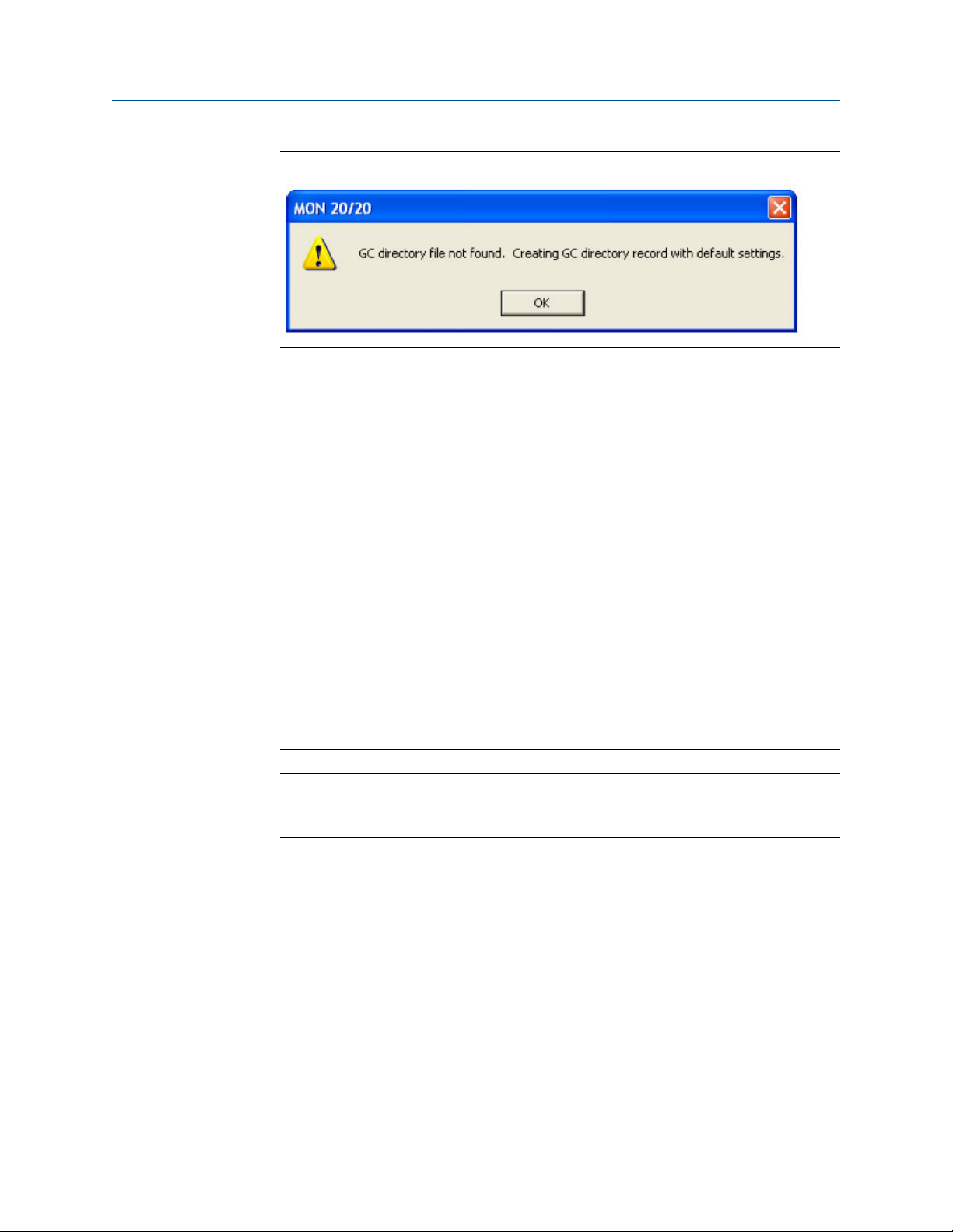
1. Select GC Directory... from the File menu.

If this is the first time that this option was selected, you will get the following error message:

Getting started

“GC directory file not found” messageFigure 1-1:

If you get the “GC directory file not found” message, click OK. The GC Directory window appears and displays a table containing an inventory of the GCs to which MON2020 can connect.

2. If you are configuring the first GC connection for MON2020, there will be only one generic GC record listed in the window. To add another record, select Add from the GC Directory window’s File menu. A new row will be added to the bottom of the table.

3. Click in the GC Name field and enter the name for the GC to which you want to connect.

4. Optionally, you can click in the Short Desc field and enter pertinent information about the GC to which you want to connect, such as its location. You can enter up to 100 characters in this field.

5. Click Ethernet. The Ethernet Connection Properties for New GC window appears.

6. In the IP address field, enter the IP address of the GC to which you want to connect.

Note

The default address for the GC's RJ-45 port in DHCP mode is 192.168.135.100.

Note

If you type in an invalid IP address, you will get an error message when MON2020 attempts to connect to the GC.

7. Click OK. When the Save changes? message appears, click Yes.

8. Repeat steps 2 through 7 for any other GCs to which you want to connect.

9. To delete a GC from the table, select the GC and then select Delete from the File menu.

10. To copy a GC's configuration information into a new row, select the row to be copied and then select Insert Duplicate from the File menu.

11. To insert a row below a GC, select the GC and then select Insert from the File menu.

12. To sort the table alphabetically, select Sort from the Table menu or click Sort from the GC Directory window.

13. To copy the list of GCs to the clipboard to be pasted into another application, select Copy Table to Clipboard from the Table menu.

Getting started

14. To print the list of GCs, select Print Table... from the Table menu.

15. To save the changes and keep the window open click Save from the GC Directory window. To save the changes and close the window, click OK. When the Save changes? message appears, click Yes.

For more details about configuring MON2020 connections, see Section 4.12.

1.2.7 Export a GC directory

The GC Directory, which contains the list of networked GCs that are currently configured for your copy of MON2020, can be saved as a DAT file to a PC or other storage media such as a compact disk or flash drive.

To save the GC Directory to the PC, do the following:

1. Click Export.

The Export GC Directory window displays.

2. Select the checkbox for each gas chromatograph whose information you want to save.

Note

If you want to save the entire list, click Select All.

Getting started

3. Click OK.

The Export GC Directory File save as dialog displays.

4. Choose a save location.

The default location is C:\Users\user_account_name\Documents\GCXA Data.

Note

The file is automatically given the name of GC_DIRECTORY_EXPORT.DAT. If you prefer a different name, type it into the File name field.

5. Click Save.

1.2.8 Import a GC Directory file

A GC Directory file can be used to restore GC directory information to your copy of MON2020, or it can be used to quickly and easily supply other copies of MON2020 that are installed on other computers with the profiles of the GCs that are in your network.

To import a GC Directory file, do the following:

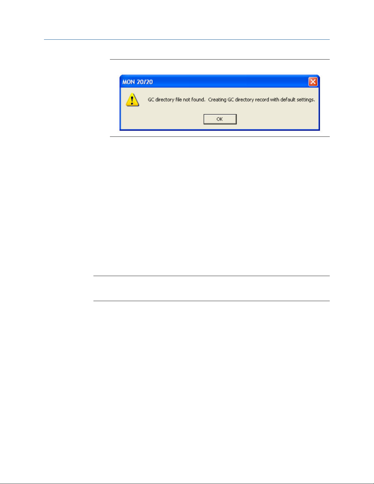
1. Select GC Directory... from the File menu.

If this is the first time that this option was selected, you will get the following error message:

Getting started

“GC directory file not found” messageFigure 1-2:

If you get the “GC directory file not found” message, click OK. The GC Directory window appears

2. Click Import.

The Import GC Directory File dialog displays.

3. Locate the GC directory file and select it.

4. Click Open.

The newly configured GC Directory window reappears with the list of networked GCs displayed in the GC Directory table.

1.2.9 Launch MON2020 from the SNAP-ON for DeltaV

This section assumes that DeltaV is installed on the PC along with MON2020.

Note

To successfully use MON2020 SNAP-ON for DeltaV, you must be familiar with using the DeltaV digital automation system.

To start MON2020, do the following:

1. Start the DeltaV Explorer by clicking on its desktop icon or by clicking the Start button and selecting DeltaV → Engineering → DeltaV Explorer.

2. In the Device Connection View, open device icons by clicking once on each icon. Follow the path of connections until you locate the desired gas chromatograph icon.

3. Right-click on a connected gas chromatograph icon to display the context menu.

4. Select SNAP-ON/Linked Apps → Launch MON2020.

MON2020 starts and connects automatically to the GC.

1.2.10 Launch MON2020 from the AMS Device Manager

This section assumes that DeltaV and AMS are installed on the PC along with MON2020.

To start MON2020, do the following:

Getting started

1. Start the AMS Device Manager by clicking on its desktop icon or by clicking the Start button and selecting AMS Device Manager → AMS Device Manager.

2. In the Device Connection View, open device icons by clicking once on each icon. Follow the path of connections until you locate the desired gas chromatograph icon.

3. Right-click on a connected gas chromatograph icon to display the context menu.

4. Select SNAP-ON/Linked Apps → Launch MON2020.

MON2020 starts and connects automatically to the GC.

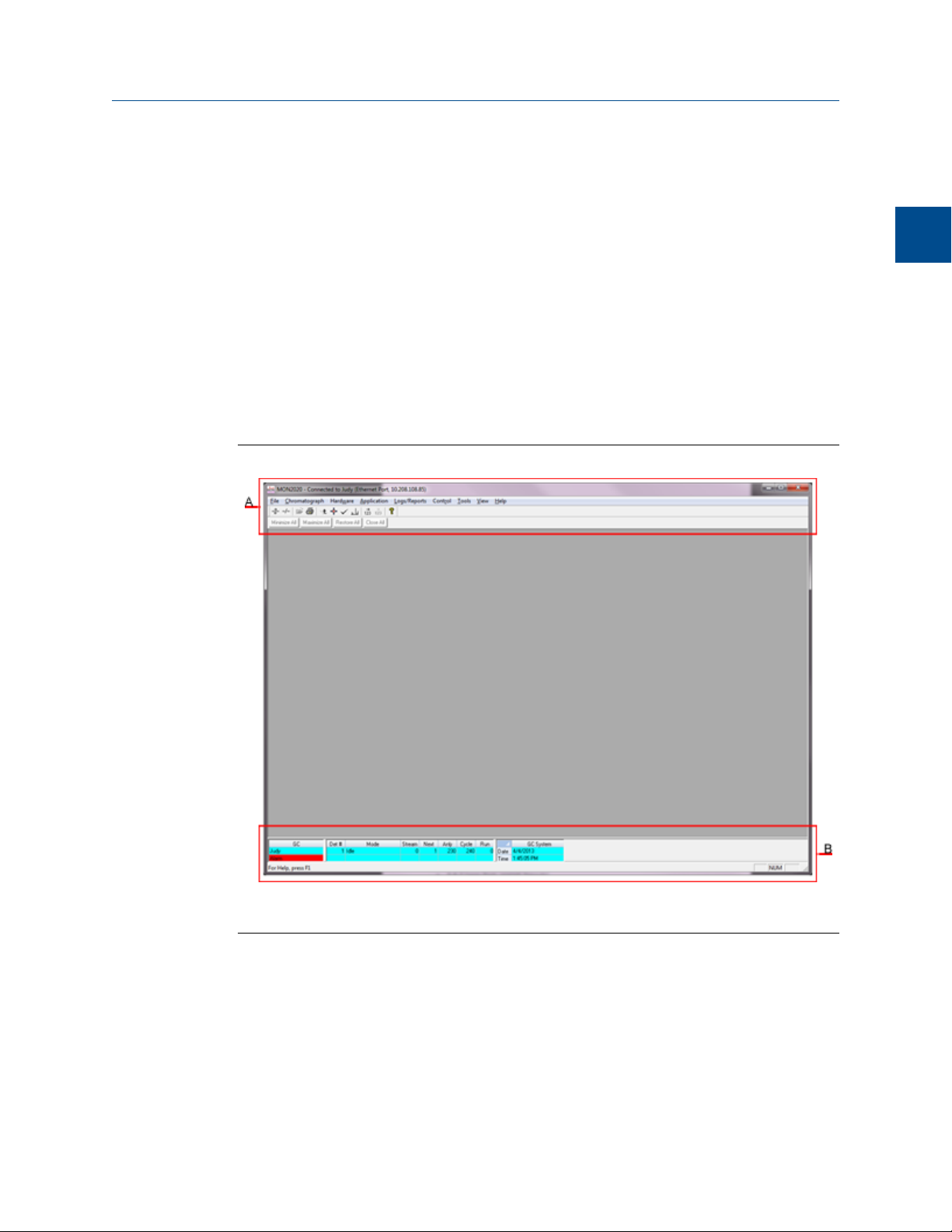
1.2.11 The MON2020 user interface

MON2020 has two areas of interaction: the Control Area, at the top of the program’s main window, and the GC Status Bar, located at the bottom of the program’s main window.

The MON2020 windowFigure 1-3:

Getting started

A. Control Area B. GC Status Bar

The main user interface

The main user interface of the main window contains the menus and icons that allow you to control MON2020 and the GC to which MON2020 is connected.

Getting started

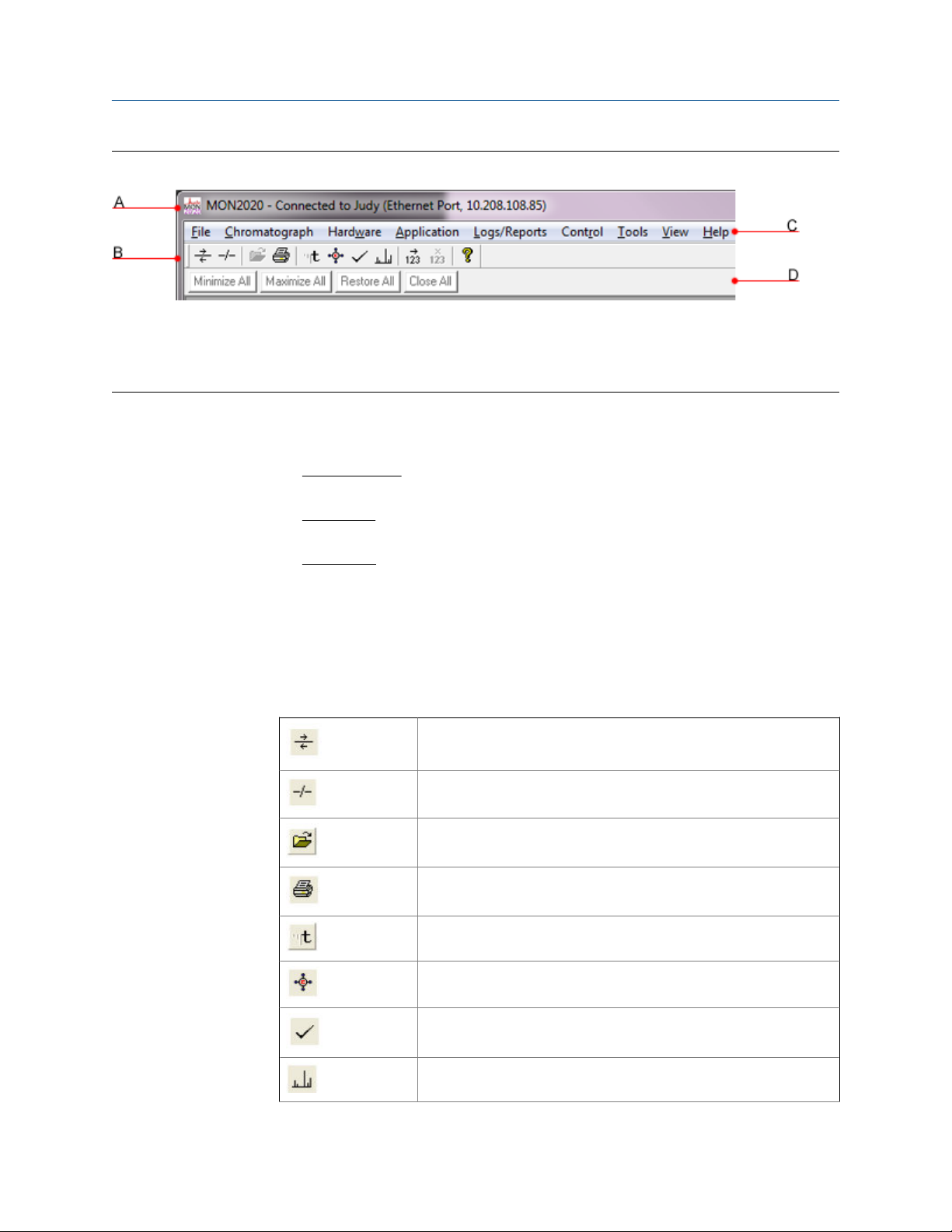
The Control AreaFigure 1-4:

A. Title bar B. Toolbar C. Menu bar D. Dialog Control Tabs

• Title bar - The Title bar displays the name of the program, as well as the program’s

• Menu bar - The Menu bar contains the commands that allow you to control and

• Toolbar - The Toolbar contains shortcut icons for the most important and/or most

connection status. MON2020 has the following three overall status modes:

- Not connected - If MON2020 is not connected to a GC, then “MON2020”

displays in the Title bar.

- Connected - If MON2020 is connected to a GC, then “MON2020 - Connected to”

and the name of the GC and the connection type displays in the Title bar.

- Offline Edit - If MON2020 is in offline edit mode, then “MON2020 - Offline Edit

<filename>” displays in the Title bar.

monitor gas chromatographs.

often used MON2020 commands. From the Toolbar you can do such things as connect to and disconnect from a GC, view chromatographs, and view help files.

Connect to a gas chromatograph.

Disconnect from a gas chromatograph.

Open a configuration file.

Print a GC configuration report.

View the Timed Events window.

View the Component Data window.

Clear or acknowledge alarms.

Open the CGM Viewer window.

Getting started

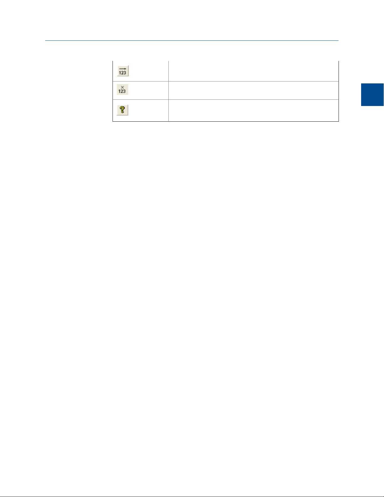
Begin auto sequencing.

Halt auto sequencing.

Open the About MON2020 window.

• Dialog Control Tabs bar - The Dialog Control Tabs bar contains four buttons that

allow you to manage the behavior of all windows that are open in the main window. The four buttons are Minimize All, Maximize All, Restore All, and Close All. The bar also displays a button for each open window that allows you to select or deselect that window.

You can hide or display the Toolbar and the Dialog Control Tabs bar by clicking the appropriate option from the View menu.

The GC Status Bar

The GC Status Bar of the main window displays useful information about the status and functioning of the gas chromatograph to which MON2020 is connected.

The GC Status Bar contains the following sections:

Getting started

GC The first row displays the name of the GC to which MON2020 is connected.

If MON2020 is not connected to a GC, “Not Connected” displays in this row. If MON2020 loses its connection to the GC, “Comm Fail” displays in this row, and the program will automatically try to reconnect. The second row displays status flags such as active alarms (with red background), unacknowledged alarms (with yellow background), or File Edit modes.

Det # A GC can have a maximum of two detectors.

Mode Potential modes are: Idle, Warmstart Mode, Manual Anly, Manual Cal,

Manual Validation, Auto Anly, Auto Cal, Auto Validation, Auto Valve Timing, Module Validation, CV Check, Manual Purge, Auto Purge, and Actuation Purge.

Stream The current stream being analyzed.

Next The next stream to be analyzed.

Anly The analysis time.

Cycle The total cycle time, in seconds, between successive analyses.

Run The amount of time, in seconds, that has elapsed since the current cycle

began.

GC System Displays the date and time according to the GC to which MON2020 is

connected. The date and time displayed may be different from the user’s date and time, depending on the physical location of the GC.

Getting started

FID Flame Status

Displays the status of the FID flame. Options are OFF with red background, ON with green background, and OVER TEMP with red background. The FID Flame Status indicator only displays on the GC Status Bar when the GC to which MON2020 is connected has an FID detector.

You can hide or display the GC Status Bar by clicking GC Status Bar from the View menu.

1.2.12 Connect to a gas chromatograph

Before connecting to a GC you must create a profile for the it on MON2020. See

Section 1.2.6 to learn how to do this.

Also, to connect to a gas chromatograph you must log on to it first. Most of MON2020’s menus and options are inactive until you have logged on to a GC.

To connect to a GC, do the following:

1. There are two ways to start the process:

On the Toolbar, click .

b. Select Connect... from the Chromatograph menu.

The Connect to GC dialog, which displays a list of all the GCs to which you can connect, appears.

Note

If you want to edit the connection parameters for one or all GCs listed in the Connect to GC window, click Edit Directory. The GC Directory window will appear. See Section 1.2.6 for more information.

2. Click the Ethernet button beside the GC to which you want to connect.

The Login dialog appears.

3. Enter a user name and user PIN and click OK.

Once connected, the name of the GC appears under the GC column in the GC Status Bar.

Note

All GCs are shipped with a default user name: emerson. A user password is not required when using this administrator-level user name. To add a user password to either of these user names or for information about creating and edit user names in general, see Section 7.3.

Note

If you enter an invalid user name or password, the Login dialog will close without connecting to the GC.

Getting started

1.2.13 Disconnect from a gas chromatograph

Disconnecting from a GC will automatically log you off of the GC.

To disconnect from a gas chromatograph, do one of the following:

•

On the Toolbar, click .

• Select Disconnect from the Chromatograph menu.

Note

If you are connected to a GC and want to connect to a different GC, it is not necessary to disconnect first; simply connect to the second GC, and in the process MON2020 will disconnect from the first GC.

1.3 Keyboard commands

You can use the following keyboard keystrokes throughout the program:

Arrow keys

Moves cursor:

• Left or right in a data field.

• Up or down in a menu or combo box.

• Up or down (column), left or right (row) through displayed data

entries.

Getting started

Delete

Enter Activates the default control element (e.g., the OK button) in current

Esc Exits application or active window without saving data.

F1 Accesses context-sensitive help topics.

Insert

Tab Moves to the next control element (e.g., button) in the window; to use Tab

Shift+Tab Moves to previous control element (e.g., button) or data field in window;

Space Toggles settings (via radio buttons or check boxes).

You can use the following function keys from the main window:

F2 Starts the Auto-Sequencing function. See Section 6.1 for more information.

• Deletes the character after cursor.

• Deletes selected rows from a table or return row values to the default

settings.

window.

• Toggles between insert and type-over mode in selected cell.

• Inserts a new row above the highlighted row.

key to move to next data field, select Program Settings... from the File menu and clear the Tab from spreadsheet to next control check box.

see Tab description.

Getting started

F3 Halts the GC (e.g., an analysis run) at the end of the current cycle. See Section 6.1 for

more information.

F5 Displays the Timed Events table per specified stream. See Section 4.3 for more

information.

F6 Displays the Component Data table per specified stream. See Section 4.2 for more

information.

F7 Displays the chromatogram for the sample stream being analyzed. See Section 2.1.2

for more information.

F8 Displays any chromatogram stored in the GC Controller. See Section 2.1.3 for more

information.

1.4 Procedures guide

Use the following table to look up the related manual section, menu path and, if appropriate, the keystroke for a given procedure.

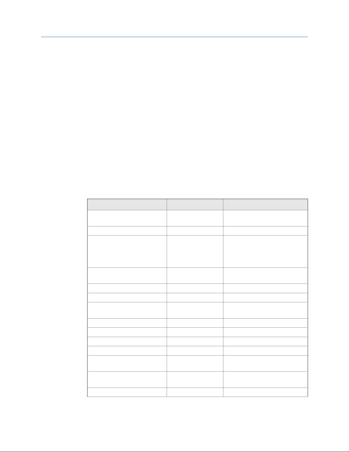
MON2020 Task ListTable 1-1:

Task or Data Item Section(s) Menu Path [Keystroke]

24-hour average, component(s) measured

Add a gas chromatograph Section 1.2.6 File → GC Directory

Alarms, related components Section 4.2

Alarms, stream number(s) programmed

Analysis Report (on/off) Section 5.7.3 Logs/Reports → Printer Control...

Analysis time Section 4.3.4 Application → Timed Events... [F5]

Starting or ending auto-calibration

Auto-calibration interval Section 4.9 Application → Streams...

Auto-calibration start time Section 4.9 Application → Streams...

Autocal time Section 4.9 Application → Streams...

Baseline Section 4.9 Application → Streams...

Base pressure used for calculations

Calibration concentration Section 4.2 Application → Component Data...

Calibration cycle time Section 4.3.4 Application → Timed Events... [F5]

Section 4.5.2 Application → Calculations → Aver-

ages...

Application → Component Data...

Section 4.7

Section 3.5

Section 4.7 Application → Limit Alarms → User...

Section 4.9 Application → Streams...

[F6]

Application → Limit Alarms → User...

Hardware → Discrete Outputs...

[F6]

Getting started

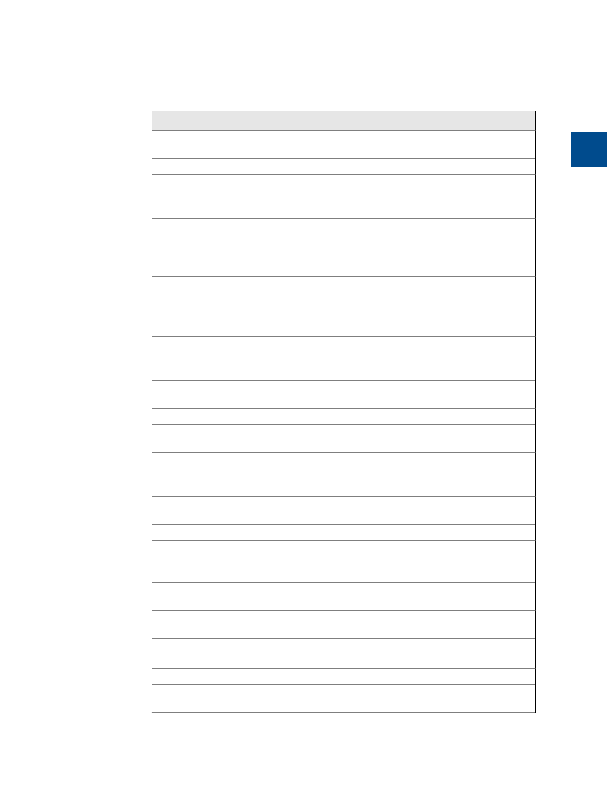
MON2020 Task List (continued)Table 1-1:

Task or Data Item Section(s) Menu Path [Keystroke]

Calibration runs, number averaged

Calibration runs, number of Section 4.9 Application → Streams...

Calibration stream number Section 4.9 Application → Streams...

Change the default C6+ mixture ratio

Communications Section 4.11 Application → Communication...

Component code and name Section 4.2 Application → Component Data...

Component full scale (for output) Section 4.1

Component(s) programmed for input

Component(s) programmed for output

Component, retention time Section 4.2 Application → Component Data...

Component zero (for output) Section 3.7 Hardware → Analog Outputs...

Compressibility (on/off) Section 4.5.1 Application → Calculations → Con-

Configure the valve timing Section 6.5 Control → Auto Valve Timing...

Current date Section 2.6 Chromatograph → View/Set GC

Current time Section 2.6 Chromatograph → View/Set GC

Cycle time Section 4.3.4 Application → Timed Events... [F5]

Delete alarms Section 4.7

Delete component from component list

Delete inhibit, integration, peak width

Delete output(s) Section 3.7

Enable or disable multi-user write Section 4.1 Application → System...

Existing alarm(s) Section 5.1 Logs/Reports → Alarms → Alarm

Section 4.9 Application → Streams...

Section 4.2.6 Application → Compnent Data Ta-

ble...

Application → Ethernet Ports...

[F6]

Application → System...

Section 3.7

Section 3.6

Section 3.4

Section 4.7

Section 3.7

Section 3.5

Section 5.1

Section 4.2 Application → Component Data...

Section 4.2 Application → Timed Events... [F5]

Section 3.5

Hardware → Analog Outputs...

Application → Analog Inputs...

Application → Discrete Inputs...

Application → Limit Alarms → User...

Hardware → Analog Outputs...

Hardware → Discrete Outputs...

[F6]

trol...

Time...

Application → Limit Alarms...

Logs/Reports → Alarms → Alarm Log...

[F6]

Hardware → Analog Outputs...

Hardware → Discrete Outputs...

Log...

Getting started

MON2020 Task List (continued)Table 1-1:

Task or Data Item Section(s) Menu Path [Keystroke]

Full-scale value (for input) Section 3.6 Hardware → Analog Inputs...

Generate a repeatability certificate

GPM liquid equivalent (on/off) Section 4.5.1 Application → Calculations → Con-

Height or area measurement method

High alarm Section 4.7 Application → Limit Alarms → User...

(Analyzer) I.D. Section 4.1 Application → System...

Inhibit on-off times Section 4.3.4 Application → Timed Events... [F5]

Input(s) being used Section 3.6

Integration on-off times Section 4.3.4 Application → Timed Events... [F5]

Low alarm Section 4.7 Application → Limit Alarms → User...

Manage the GC's pressure Section 3.3 Hardware → EPC...

Mole percent (on/off) Section 4.5.1 Application → Calculations → Con-

Normalization (on/off) Section 4.5.1 Application → Calculations → Con-

Outputs being used Section 4.7

Peak width, on time Section 4.3.4 Application → Timed Events... [F5]

Relative density (on/off) Section 4.5.1 Application → Calculations → Con-

Response factor Section 4.2 Application → Component Data...

Response factor, percent deviation

Retention time, percent deviation Section 4.2 Application → Component Data...

Spectrum gain Section 4.3.3 Application → Timed Events... [F5]

Stream number(s) (for output) Section 4.7

Stream sequences skipped, number

Streams analyzed, number Section 4.1

Section 5.12 Logs/Reports → Repeatability Certif-

icate...

trol...

Section 4.2 Application → Component Data...

[F6]

Hardware → Analog Inputs...

Section 3.4

Section 3.7

Section 3.5

Section 4.2 Application → Component Data...

Section 3.7

Section 3.5

Section 4.1

Section 4.9

Hardware → Discrete Inputs...

trol...

Application → Limit Alarms → User...

Hardware → Analog Outputs...

Hardware → Discrete Outputs...

trol...

[F6]

Application → Limit Alarms → User...

Hardware → Analog Outputs...

Hardware → Discrete Outputs...

Application → System...

Application → Streams...

Application → System...

Application → Streams...

Getting started

MON2020 Task List (continued)Table 1-1:

Task or Data Item Section(s) Menu Path [Keystroke]

Streams analyzed, sequence Section 4.1

Section 4.9

Valve on/off times Section 4.3.1 Application → Timed Events... [F5]

Weight percent (on/off) Section 4.5.1 Application → Calculations → Con-

Wobbe value (on/off) Section 4.5.1 Application → Calculations → Con-

Zero value (for input) Section 3.6 Hardware → Analog Inputs...

1.5 Configuration files

Use the File menu to edit, save, and restore configuration files.

1.5.1 Edit a configuration file

To edit a configuration file, do the following:

Application → System...

Application → Streams...

trol...

Getting started

1. Disconnect from the GC.

2. Select Open Configuration File... from the File menu.

The Open dialog displays. Configuration files are saved with the .xcfg extension.

3. Locate and select the configuration file that you want to edit and click Open.

MON2020 opens the file in offline edit mode.

4. Use the Application and Hardware menu commands to edit the configuration file. For more information on these commands, see Chapter 3 and Chapter 4.

5. When finished editing the configuration file, click

configuration file and to leave offline edit mode.

1.5.2 Save the current configuration

Configuration files are saved with the .xcfg extension. To save a GC’s current configuration to a PC, do the following:

1. Select Save Configuration (to PC)... from the File menu.

The Save as dialog displays.

to save the changes to the

2. Give the file a descriptive name or use the pre-generated file name and navigate to the folder to which you want to save the file.

Getting started

3. Click Save.

1.5.3 Import a configuration file

CAUTION!

The current configuration will be overwritten, so be sure to save it before importing a new or previous configuration. See Section 1.5.2 to learn how to save a configuration.

CAUTION!

The GC must be in Idle mode while performing this task.

To import a configuration into a GC, do the following:

1. Select Restore Configuration (to GC)... from the File menu.

The Open dialog displays. Configuration files are saved with the .xcfg extension.

2. Locate and select the configuration file that you want to import and click Open.

The file’s data is loaded into the GC.

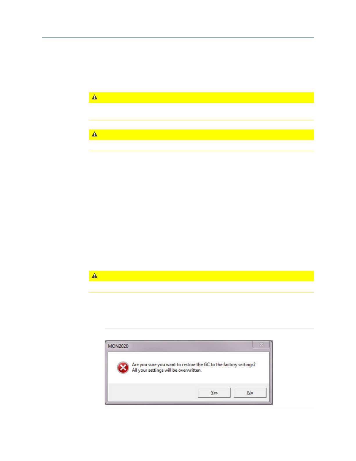
1.5.4 Restore the GC's factory settings

The GC’s default timed event, component data and validation data tables are created at the factory and are not accessible by users. To restore these tables to their default values, do the following:

CAUTION!

The GC must be in Idle mode while performing this task.

1. Select Restore to Factory Settings... from the File menu.

The following warning message displays:

Restore to Factory Settings warning messageFigure 1-5:

Getting started

2. Click Yes.

MON2020 restores the default values to the GC’s data tables. When the process is completed, a confirmation message displays.

3. Click OK.

1.6 Configure your printer

Select Print Setup... from the File menu to configure the settings for the printer connected to your PC. These settings will apply to any print job queued from MON2020, such as the reports that are configured by the Printer Control. See Section 5.7.3 for information.

The settings available depend on the printer model. Refer to the printer manufacture’s user manual for more information.

Note

Your new configuration will be cleared, i.e., the settings will return to the default values, when you exit MON2020.

Getting started

1.7 Online help

Currently, the online help feature contains all user information and instructions for each MON2020 function as well as the MON2020 system.

To access the online help, do one of the following:

• Press F1 to view help topics related to the currently active dialog or function.

• Select Help Topics from the Help menu to view the help contents dialog.

1.8 Operating modes for MON2020

The GC supports two different operating modes. Each mode allows the GC to analyze data from a given number of detectors, streams, and methods, as detailed in below.

Operating Modes for MON2020Table 1-2:

Mode ID Number Detectors Supported Streams Supported Methods Supported

0 1 1 1

1 2 1 1

Getting started

1.9 The Physical Name column

Most MON2020 hardware windows, such as the analog inputs or the valves, contain a hidden column called Physical Name that lists the default name of the associated GC device. It might be useful to know a device’s physical name while troubleshooting.

To view the hidden column, do the following:

1. Select Program Settings... from the File menu.

The Program Settings window displays.

2. Select the Show Physical Names checkbox.

3. Click OK.

The Physical Name column now will be visible on all windows that have the column, such as the Heater window or the Valves window.

1.10 Select the GC’s networking protocol

MON2020 can connect to the GC using one of two networking protocols: PPP or SLIP. If the version level of the GC’s firmware is 1.2 or lower, MON2020 should be configured to use the SLIP protocol; otherwise, the PPP protocol should be used.

To select the GC’s networking protocol, do the following:

1. Select Program Settings... from the File menu.

The Program Settings window displays.

2. To use the PPP protocol, make sure the Use PPP protocol for serial connection (use SLIP

if unchecked) checkbox is selected; to use the SLIP protocol, make sure the Use PPP protocol for serial connection (use SLIP if unchecked) checkbox is not selected.

3. Click OK.

1.11 The context-sensitive variable selector

The MON2020 method for selecting variables for calculations and other purposes is based on a simple, self-contained system.

Getting started

Example of a context-sensitive variable selectorFigure 1-6:

The context-sensitive variable selector consists of a first-level element, called the context element, that is followed by a series of tiered, drop-down lists. The options available from

the drop-down lists depend upon the context element.

The following example explains how to use the context-sensitive variable selector to select a user alarm variable:

1. Click on the second-level drop-down list.

The full list of available streams displays.

2. Select the stream you want to use for the alarm.

3. Click the third-level drop-down list.

Getting started

The full list of available user alarm variables displays.

4. Select the variable you want to use for the alarm.

If there are components associated with the variable, the fourth-level drop-down list will display.

5. If displayed, click the fourth-level drop-down list.

The full list of available components displays.

6. Select the component you want to use for the alarm.

7. Click [Done].

The context-sensitive variable selector closes and the variable displays in the Variable field.

Getting started

2 Chromatograph

When it comes to viewing and managing chromatograms, MON2020 is flexible and straightforward. This chapter shows you how to access the Chromatogram Viewer, as well as how to use the viewer to display, print, and manipulate live, archived, or saved chromatograms. There is no limit to the number of archived and saved chromatograms that can be displayed at once. The Chromatogram Viewer can display all three types of chromatograms together, alone, or in any combination.

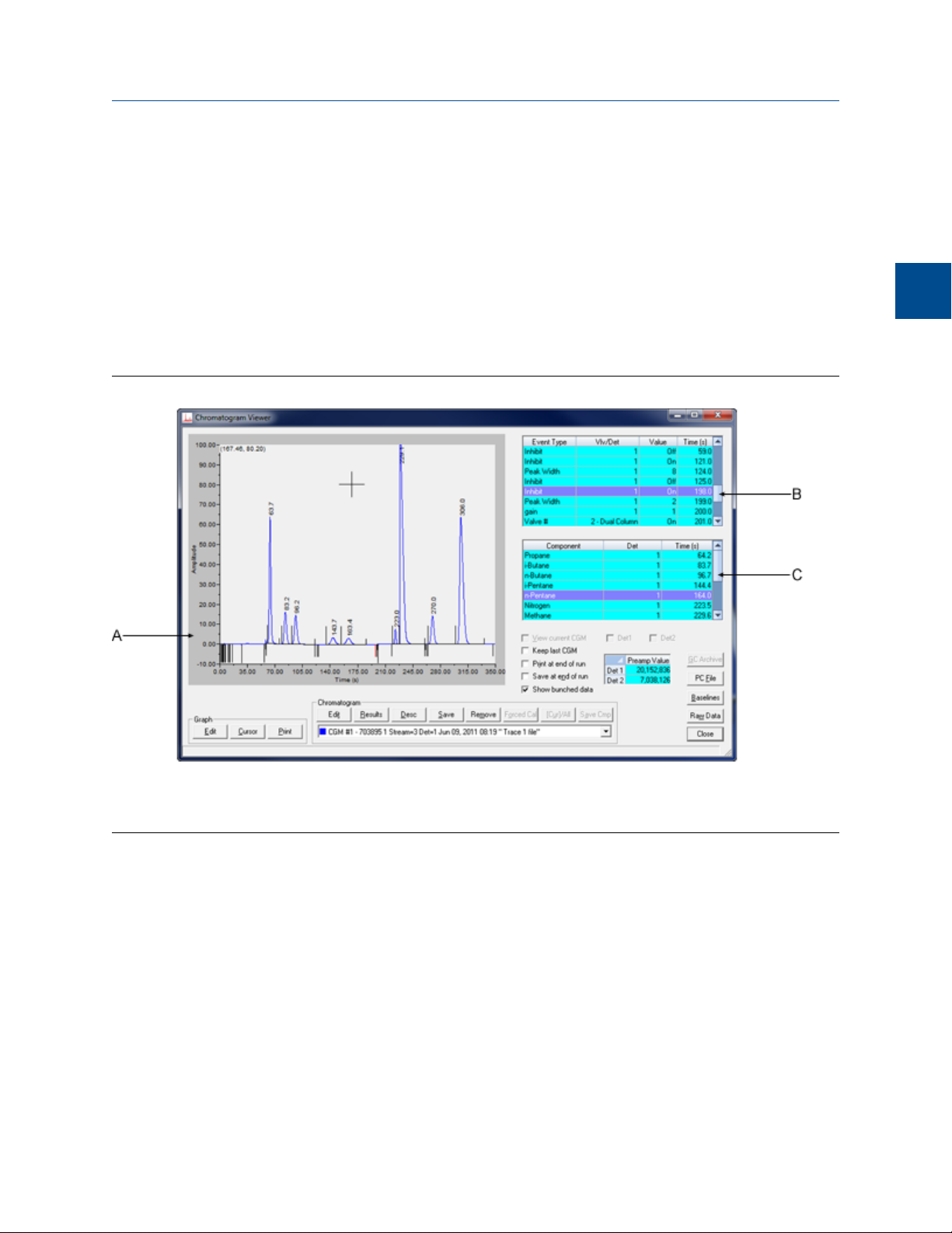
The Chromatogram ViewerFigure 2-1:

Chromatograph

A. Chromatogram window B. Time events table C. Component data table

A chromatogram displays in the chromatogram window. If the chromatogram contains one trace, the Det1 checkbox is automatically checked; if the chromatogram contains two traces, the Det1 and Det2 checkboxes are automatically checked. To remove a trace, uncheck its detector checkbox.

Each trace that displays is color-coded; use the Chromatogram pull-down menu to select a specific trace.

Chromatograph

Chromatogram pull-down menuFigure 2-2:

The list of GC events associated with the production of the chromatogram, along with each event’s status and time, displays in the Timed Events table to the right of the chromatogram display window. The Component Data table, to the lower right of the chromatogram display window, lists the components measured during the analysis. These tables are updated in real-time, just as the chromatogram is.

Note

By default, the timed events and component data tables are configured to scroll to and highlight the next occurring event in the analysis cycle. To disable this feature, right-click on one of the tables and uncheck the Auto Scroll option on the pop-up menu.

2.1 The Chromatogram Viewer

Use the Chromatogram Viewer to display and print live, archived, or saved chromatograms. There is no limit to the number of archived and saved chromatograms that can be displayed at once; however, to maximize performance, the number of chromatograms displayed should be limited to 25 or less. The Chromatogram Viewer can display all three types of chromatograms together, alone, or in any combination.

The Chromatogram Viewer contains a host of information about both current and past GC analyses, and it contains just as many ways of editing and manipulating that data.

2.1.1 Data displayed in the chromatogram window

Chromatograph

The chromatogram windowFigure 2-3:

Chromatograph

A. Retention time B. Peak detection marker C. Timed event marker

The following elements are displayed in the chromatogram window:

The chromatogram

Retention times The retention time, which displays above each component's peak,

Baselines The baseline extends from the beginning to the end of a peak. You

Timed event markers

A trace is the graphical representation of the detector output from a single detector; a chromatogram is the collection of all traces and associated data that are generated by a gas chromatograph’s detector or detectors. Each trace displays in a different color.

is the time that elapses between the start of an analysis and the sensing of the maximum concentration of that component by the detector.

can turn the baseline on or off by clicking Baselines.

These markers, which correspond to events from the Timed Events table, display on the chromatogram as black vertical lines below the trace-line. There are three types of timed event markers:

• Valve events display as long vertical lines.

• Integration events display as medium vertical lines.

Chromatograph

• Spectrum gain events display as short vertical lines.

Peak detection markers

These markers display on the chromatogram as black vertical lines above the trace-line. Each peak has two peak detection markers: one at its beginning and one at its end.

2.1.2 Display a live chromatogram

To view a live chromatogram, do the following:

1. Connect to the GC.

2. Select Chromatogram Viewer... from the Chromatograph menu.

Note

Another way to display the Chromatogram Viewer is to click , which is located on the Toolbar.

3. From the Chromatogram Viewer window, select the View current CGM check box.

2.1.3 Display an archived chromatogram

Archived chromatograms are stored on the GC, so you must be logged in to access them.

Archived chromatograms are sorted and displayed on four tabbed panes:

Chromatograms This view displays all chromatogram types sorted by time so that

the newest file is always listed first. This view can be further configured to display only the files from the last five runs for each stream, or to display all the files that are stored on the GC.

Protected chromatograms

Final Calibration chromatograms

Protected chromatograms are never deleted from the GC. To protect a chromatogram, see Section 2.1.4.

Note

Protected chromatogram files have a “lock” icon ( ) displayed beside them.

As long as there is space, MON2020 will store all final calibration chromatograms; once space runs out, MON2020 will delete the oldest non-protected final calibration chromatogram for each new final calibration chromatogram that is created. If multiple final calibration chromatograms are created on the same day, the last chromatogram created is archived, unless MON2020 has been configured to archive all final calibration chromatograms.

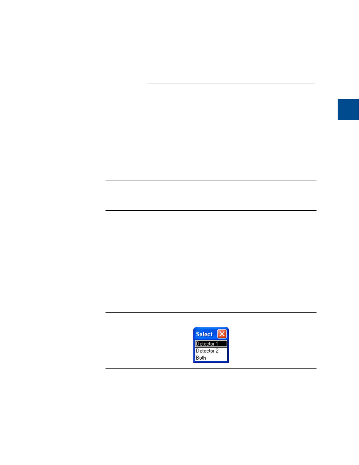
Note

See Section 4.1 to learn how to configure MON2020’s archiving behavior.

Final Validation chromatograms

These chromatograms are treated in the same manner as final calibration chromatogram files.

To view one or more archived chromatograms, do the following:

1. Click GC Archive.

The Select archive file(s) window appears. The files can be sorted by date, file name, analysis type, time, or stream number by clicking the appropriate column header. By default, they are sorted by date, with the newest file listed first.

Note

By default, only recent chromatograms—that is, the last five runs for each stream—are displayed. To view all archived chromatograms, click All. To return to viewing only recent chromatograms, click Recent.

Chromatograph

2. Select one or more archive files by clicking them.

Use the SHIFT and CTRL keys to make multiple selections.

Note

To save the selected files to the PC without displaying them first, select the Download and save selected chromatograms check box and click Download & Save.

3. Click Download & Show.

The Select window displays for each chromatogram that contains data from more than one detector.

The Select windowFigure 2-4:

4. For each chromatogram, double-click either “Detector 1”, “Detector 2”, or “Both” from the Select window.

MON2020 plots the archived chromatogram(s) and the corresponding data displays in the timed event and component data tables.

Chromatograph

2.1.4 Protected chromatograms

By default, archived chromatograms are not saved indefinitely. Once the GC’s storage capacity for archived chromatograms has been reached, the oldest archived chromatograms are deleted to make room for the newest archived chromatograms.

If you have a chromatogram that you would like to preserve, it is possible to "protect" it. Protected chromatograms will not be deleted to accommodate newer chromatograms. To delete a protected chromatogram, it must first be unprotected. See

Unprotect a protected chromatogramfor more information. MON2020 will save up to 100

protected chromatograms.

Note

Protected chromatograms have a “lock” icon ( ) displayed beside them.

Note

To protect an archived chromatogram you must be logged in as a supervisor or administrator. To protect a chromatogram, do the following:

1. Click GC Archive.

The Select Archive File(s) window appears. The chromatograms can be sorted by date, file name, analysis type, time, or stream number by clicking the appropriate column header. By default, they are sorted by date, with the newest chromatogram listed first.

Note

2. Make sure the Chromatogram tab is selected and then select the appropriate archived chromatogram by clicking it. Use the SHIFT or CTRL key to make multiple selections.

3. Click Protect.

The Edit Description window displays.

4. Enter any information that you would like to have associated with the chromatogram and then click OK. If you do not want to enter any information, click Cancel.

MON2020 will place a “lock” icon ( ) beside the selected chromatogram to verify its protected status. You can also click on the Protected Chromatograms tab to view your newly protected archived chromatogram.

2.1.5 Display a saved chromatogram

To view a chromatogram that was saved to disk, do the following:

Chromatograph

1. Click PC File.

The Open dialog appears.

2. Navigate to the desired .xcgm file or .xcmp comparison file and select it.

To make multiple selections, use the SHIFT or CTRL key.

3. Click OK.

The Select window displays for each chromatogram that contains data for more than one detector.

The Select windowFigure 2-5:

4. For each chromatogram, double-click either “Detector 1”, “Detector 2”, or “Both” from the Select window.

MON2020 plots the archived chromatogram(s) and the corresponding data displays in the timed event and component data tables.

Chromatograph

2.2 Options for displaying chromatograms

Right-clicking on the graph brings up the following commands:

Command Name Shortcut Description

Zoom In “+” (NUMPAD) Zooms in on the entire graph.

Note: Another way to zoom in is by clicking and dragging your mouse to select

the region of the graph that you want to zoom in on.

Zoom Out “-” (NUMPAD) Zooms out from the entire graph.

Zoom X In “6” (NUMPAD) Zooms in on the X axis.

Zoom X Out “4” (NUMPAD) Zooms out from the X axis.

Zoom Y In “8” (NUMPAD) Zooms in on the Y axis.

Zoom Y Out “2” (NUMPAD) Zooms out from the Y axis.

Chromatograph

Command Name Shortcut Description

Save State CTRL + HOME Saves current or archived display settings for the selected chromatogram.

Note: The Save State function is available only when viewing a live or archived chromatogram.

Restore State HOME Restores the last saved display settings for the selected chromatogram.

Note: Pressing HOME returns the user to the saved state.

Toggle Full Screen F11 Toggles the display of the Chromatogram Viewer’s tables and buttons and

maximizes the chromatogram window.

Cursor to Nearest Point

Toggle Coarse/Fine Cursor

Toggle Lines/Dots Displays

Toggle Mouse Position Tip

Toggle Nearest Position Tip

Print CTRL + P Prints the chromatogram.

Copy to clipboard CTRL + C Copies from the graph the raw detector data that was used to plot the selected

Paste from clipboard

F8 Snaps the cursor to the nearest point on the chromatograph in both the X and

Y directions.

F4 Toggles the cursor from coarse and less accurate to fine and more accurate.

F9 Toggles the chromatographs from lines to dots, or dots to lines.

CTRL + F4 The graph’s cursor follows the movement of the mouse while a hovering tool-

tip displays the exact coordinates of the current point.

CTRL + F9 The graph’s cursor follows the movement of the mouse cursor.

chromatogram. This data can be pasted into another application such as Microsoft Word or Microsoft Excel.

CTRL + V Plots a range of points copied from another application such as Microsoft Word

or Microsoft Excel.

2.3 Configure the appearance of the chromatograph

MON2020 allows you to change the appearance of many of the chromatogram’s elements, such as its x-axis and y-axis values, the color of the chromatograph’s background, and the display status of its labels.

2.3.1 The Graph bar

Use the Graph bar buttons to change the display parameters of the chromatogram.

Click Edit from the Graph bar. The Edit Scales window displays.

The following table lists the parameters that can be edited:

Chromatograph

Command Description

X Min Sets the minimum value, in seconds, for the X axis. 0

X Max Sets the maximum value, in seconds, for the X axis. The is value is

determined by the Timed Events table.

Y Min Sets the minimum value for the Y axis. -10

Y Max Sets the maximum value for the Y axis. 100

Print Speed Sets the number of inches per second for the x-axis while printing a

chromatogram, similar to an XY plotter.

X Intervals Sets the number of intervals to be displayed on the graph for the X

axis.

Y Intervals Sets the number of intervals to be displayed on the graph for the Y

axis.

Display Option

Show labels Toggles the display of the graph labels. Checked

Scroll newestXDetermines whether the graph’s window moves to focus on the

Determines whether the chromatograph is displayed as a solid line or as a dotted line. Lines is checked by default.

most recent data point along the x axis. This feature only applies to live chromatograms.

Default Value

100

Lines

Unchecked

Chromatograph

A chromatographFigure 2-6:

To see how your changes affect the graph, click Apply. To accept your changes, click OK.

• Click Cursor to toggle the cursor size from coarse movement (less accurate) to fine

movement (more accurate).

• Click Print to print the chromatogram window.

2.3.2 Additional plot commands

In addition to the Graph bar, there are a few other commands available that allow you to manipulate the look and feel of the graph. To access the additional plot commands menu, right-click on the Chromatogram Viewer anywhere except on the graph or the timed event and component data tables. The additional commands are:

Set Plot Area Color

Auto Resize Series

Changes the color of the graph’s background. This may be necessary to make the chromatograms more visible. The default RGB color values are 236, 233, and 216.

Scales down the X-axis and the Y-axis to fit the entire chromatogram onto the window.

Chromatograph

Show Mini Plot

Rearrange Series

Trace Offset Settings

Toggles the display of a smaller version of the chromatogram in a separate, smaller, and resizable window. This allows you to keep an overview of the entire graph at all times, especially when zoomed in.

This window automatically displays whenever you zoom in on the original chromatogram.

Resizes and offsets two or more traces so that they can both be fully displayed on the graph. To offset a trace means to raise its Y-axis relative to the Y-axis of the previous trace so that one trace is not drawn over the other but instead one trace is drawn above the other.

Indicates the amount of offset between two or more traces. To offset a trace means to raise its Y-axis relative to the Y-axis of the previous trace so that one trace is not drawn over the other but instead one trace is drawn above the other.

If two detectors are in use, each set of traces can be offset independently--that is, the traces for one detector can be offset relative to each other, but independent of the traces from the second detector.

2.4 Change how a chromatogram displays

The Chromatogram barFigure 2-7:

Chromatograph

The Chromatogram bar contains a row of buttons that allows you to manipulate a single chromatogram. Below the row of buttons is the Chromatogram bar's pull-down menu, which contains a list of all of the currently displayed chromatograms/traces. Before you can work with a chromatogram you must first select it from the pull-down menu.

2.4.1 Edit a chromatogram

You can use the Edit function to change the X and Y offset values for a trace, as well as its color. These changes may be necessary to make the trace more distinguishable from those that surround it, or to align a trace with a different trace for comparison.

To edit a trace, do the following:

1. Select the trace that you want to edit from the Chromatogram pull-down menu.

2. Click Edit.

The Edit Chromatogram dialog appears.

Chromatograph

X Offset Enter a positive number to move the trace to the right, or a negative

number to move the trace to the left.

Y Offset Enter a positive number to move the trace up, or a negative number to

move the trace down.

# points Number of data points in the trace. This field is read-only.

Color Assigns a color to the trace.

3. To see how your changes affect the trace, click Apply. To accept your changes, click

OK.

2.4.2 Display chromatogram results

To display a table of calculation results for a chromatogram, do the following:

1. From the Chromatogram bar's pull-down menu, select the appropriate trace.

2. Click Results.

A window appears displaying the calculation results for the selected trace.

• Click Save to save these results in one of the following formats: tab-delimited (.txt),

comma-delimited (.csv), Microsoft Excel (.xls), HTM (.htm), or XML (.xml).

• Click Clipboard to copy the data to the Windows® clipboard, where it can be pasted

into another document.

• Click Print to print a tab-delimited version of the results.

2.4.3 Save a chromatogram

To save a chromatogram, do the following:

1. From the Chromatogram bar's pull-down menu, select the trace that you want to

save.

2. Click Save.

The Save As window displays.

For convenience the file is given an auto-generated file name that includes the trace’s creation date and time; however, you can give the file any name that you choose.

3. Click Save.

2.4.4 Remove a chromatogram from the Chromatogram

Viewer

To remove a live trace from the chromatogram window, do one of the following:

• If you want to remove all live traces, click the View current CGM check box to uncheck

it.

• If you want to remove a single live trace, click the appropriate detector checkbox

beside the View current CGM check box.

To remove a saved or an archived chromatogram from the chromatogram window and to close the file, do the following:

1. From the Chromatogram bar's pull-down menu, select the trace that you want to

remove.

2. Click Remove.

2.4.5 Initiate a forced calibration

The Forced Cal command uses an archived chromatogram’s raw data to calibrate the GC. The calculation results are stored in the component data table for the corresponding stream number.

A major benefit of a forced calibration is increased efficiency. Using a previously validated chromatogram removes the necessity for the GC to perform a calibration and a validation before performing an analysis.

To perform a forced calibration, do the following:

Chromatograph

1. From the Chromatogram bar's pull-down menu, select the trace that you want to

use to calibrate the GC.

2. Click Forced Cal.

2.4.6 Chromatogram Viewer tables

MON2020 can display two levels of information in the Chromatogram Viewer's timed events and component data tables:

• All timed events and all components for all open chromatograms.

• Timed events and components for the currently selected chromatogram.

By default, the two tables show only the timed events and components for the currently selected chromatogram.

Chromatograph

Figure 2-8:

Figure 2-9:

Timed events and component data tables showing data for a currently selected trace

Timed events and component data tables showing data for all open traces

Note

The brackets ([ ]) on the Cur/All button indicate which mode is being displayed in the tables.

1. To view the data for a different chromatogram, select the trace from the

Chromatogram bar's pull-down menu.

2. To view all timed events and all components for all open chromatograms, click Cur/

All.

3. To toggle back to viewing only the timed events and components for the currently

selected chromatogram, click Cur/All again.

2.4.7 Open a comparison file

A comparison file contains two or more chromatograms and their associated data. To open a comparison file, do the following:

1. Click PC File. The Open dialog displays.

2. Select XA CMP Files (*.xcmp) from the Files of type drop-down menu.

3. Navigate to the folder that contains the comparison file that you want to open and

select the file.

4. Click Open.

2.4.8 Save a comparison file

A comparison file allows you to save your current view, including all open chromatograms, for later review and reuse. To save a comparison file, do the following:

1. Click Save Cmp.

The Save As dialog appears.

Chromatograph

2. Navigate to the folder in which you want to save the file.

Note

For convenience the file is given an auto-generated file name that includes the current date and time; however, you can give the file any name that you choose.

3. Click Save.

2.5 Miscellaneous commands

The series of check boxes to the right of the graph have the following functions:

Miscellaneous optionsFigure 2-10:

Keep last CGM When viewing a live chromatogram, upon starting a new run,

MON2020 keeps the most recently completed chromatogram on the graph for comparative purposes.

Chromatograph

Print at end of run

Save at end of run

Show bunched data

Prints the chromatogram to the PC's default printer at the end of the run and is unchecked by default.

Saves the chromatogram to the GC's Data folder at the end of the run and is unchecked by default.

If this box is unchecked, then all of the raw data points are plotted to the chromatogram window; if this box is checked, which is the default option, then each point plotted on the graph represents the average of a group of raw data values. The size of the data group is determined by the peak width value listed in the Timed Events table.

2.5.1 The Chromatogram Viewer's Timed Events table

The Chromatogram Viewer displays a compact version of the Timed Events table, located on the upper right side of the window. The events displayed in the table are sorted by time. See Section 4.3 for more information.

The Timed Event table displays the following data for each event:

Event Type The type of timed event. These events are mapped to the Time Events

window and include Valve, Integration and Gain events.

Vlv/Det Identifies which valve or detector is involved in the event.

Value Setting of the event; for example, a valve was turned ON, or the gain was

set to 4.

Time (s) The number of seconds into the cycle that the event occurred or will occur.

Timed events from live or archived chromatograms can be edited from the Chromatogram Viewer by double-clicking on the Timed Events table. The changes will affect the next analysis run. The following commands are available by right-clicking on the table:

Auto Scroll When checked, if a live trace has been selected from the

Chromatogram bar's pull-down menu, the Timed Event table will keep its focus on the event closest in time by highlighting that event in dark blue.

Save Sheet Allows you to save the table to the PC in one of the following formats:

TXT, CSV, XLS, HTM, or XML.

Copy to Clipboard

Allows you to copy the table to the clipboard. This data can be pasted into another application such as Microsoft

Word or Microsoft Excel.

Print Sheet Allows you to print the table to your default printer.

Chromatograph

2.5.2 Launch the Timed Events table from the Chromatogram Viewer

To launch the Timed Events dialog directly, right-click on the Chromatogram Viewer’s Timed Events table and select Edit Timed Events Table. The Timed Events dialog displays. See Section 4.3 for more information.

2.5.3 Edit Timed Events from the Chromatogram Viewer

To edit timed events from the Chromatogram Viewer, do the following:

1. From the Chromatogram bar's pull-down menu, select the chromatogram whose

timed events you want to edit.

2. Right-click on the Timed Events table and select Edit.

The cells that can be edited turn white.

3. Edit the appropriate event.

4. Right-click on the Timed Events table and select Save Changes.

The data will be saved and the table's cells will turn blue, indicating that they are read-only. The changes will affect the next analysis run.

Chromatograph

Note

To return to the Timed Events table without saving your changes, select Discard Changes.

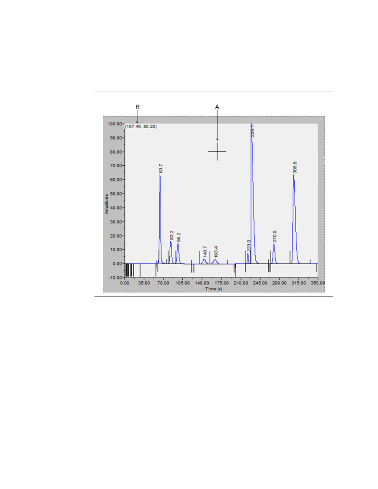
Chromatograph

2.5.4 Use the Chromatogram Viewer’s cursor to update a Timed Event

Chromatograph cursorFigure 2-11:

The Chromatogram Viewer's cursor (A) can be dragged to any point on the graph, or it can be relocated by double-clicking within the boundaries of the graph.

As the cursor moves across the chromatogram, the Timed Events table automatically scrolls to the event that corresponds to the cursor’s coordinates. The cursor’s coordinates (B) display in the upper left corner of the graph.

The cursor can be useful if you want to change a timed event based on the data displayed by the chromatogram.

To update a timed event based on the location of the Chromatogram Viewer’s cursor, do the following:

1. Select the live or archived trace that you want to use as the source for changing the

timed event.

2. Drag the cursor to the desired location.

Chromatograph

You can track the cursor's location by watching the coordinates that display in the upper left corner (B). The x-coordinate represents the analysis time in seconds. When you see the desired time displayed, stop dragging the cursor.

Note

To toggle the cursor’s size between coarse movement (less accurate) and fine movement (more accurate), click the Cursor button on the Graph bar.

3. Go to the Time Events table and right-click on the appropriate event.

4. Select Update Time from Cursor.

The event’s time will be changed to match the cursor’s time (x-coordinate).

5. To save your changes, right-click on the Timed Events table and select Save

Changes.

The changes will affect the next analysis run.

Note

To return to the Timed Events table without saving your changes, select Discard Changes.

2.5.5 The Chromatogram Viewer's Component Data table

The Chromatogram Viewer displays a compact version of the Component Data table beneath the Timed Events table. See Section 4.2 for more information.

The Component Data table displays the following data for each component:

Chromatograph

Component The name of the component.

Det Identifies the detector associated with the component.

Time (s) The retention time for the component.

Retention times for components from live or archived chromatograms can be edited from the Chromatogram Viewer by double-clicking on the Component Data table. The changes will affect the next analysis run. The following commands are available by right-clicking on the table:

Auto Scroll When checked, if a live trace has been selected from the

Chromatogram bar's pull-down menu, the Component Data table will keep its focus on the component closest in time by highlighting that it in dark blue.

Save Sheet Allows you to save the table to the PC in one of the following formats:

TXT, CSV, XLS, HTM, or XML.

Copy to Clipboard

Print Sheet Allows you to print the table to your default printer.

Allows you to copy the table to the clipboard . This data can be pasted into another application such as Microsoft Word or Microsoft Excel.

Chromatograph

2.5.6 Edit retention times from the Chromatogram Viewer

To edit the retention time for a component, do the following:

1. Double-click on the Component Data table or right-click on the table and select Edit

Retention Times.

The Ret Time column turns white, indicating that its cells are editable.

2. Click on the appropriate cell for the component that you want edit, and enter a new

retention time, in seconds. The value must be less than the analysis time.

3. To save your changes, right-click on the table and select Save Changes.

The changes will affect the next analysis run.

Note

To return to the Component Data table without saving your changes, select Discard Changes.

2.5.7 Display raw data from the Chromatogram Viewer

Use the Raw Data button to display the Raw Data table for the selected trace.

1. Use the Chromatogram bar's pull-down menu to select a specific trace.

Note

Even though you are selecting a trace, the data that is displayed will be for the chromatogram, which may include more than one trace.

2. Click Raw Data.

The Raw Data window displays and shows the raw data for the selected chromatogram. The following data displays for each peak from the trace:

No. Numerical identifier for the peak, listed by the order of

discovery.

Ret Time Time, in seconds, that the component eluted.

Peak Area The area under the peak.

Peak Height The maximum height of the peak.

Det The detector associated with the peak.

Method Method of peak end detection. Options are:

• 1 (Baseline)

• 2 (Fused Peak)

• 3 (Last Fused Peak)

• 4 (Tangent Skim)

• 100 (Inhibit)

• 300 (Forced Integration)

• 500 (Summation)

Chromatograph

Integ. Start Time, in seconds, when integration started.

Integ. Stop Time, in seconds, when integration stopped.

Peak Width Half Height

Is Partial Peak If Y, then the Partial Peak value is used in the summation

The width of the peak taken at half of the peak’s height.

calculation; if N, then the Partial Peak value is not used in the summation calculation.

2.6 Set the gas chromatograph’s date and time

When MON2020 connects to a gas chromatograph, the Status Bar displays the gas chromatograph’s date and time.

Note

The date and time displayed for the GC may be different from the user’s date and time, depending on the physical location of the GC.

To set the gas chromatograph’s date and time, do the following:

1. Select View/Set Date Time... from the Chromatograph menu.

Chromatograph

The View/Set Date Time window displays.

2. Use the drop-down menus to set the date and time.

To enable or adjust daylight savings, see Section 2.6.1.

3. Click OK.

2.6.1 Set daylight savings

Daylight savings time is the practice of temporarily advancing clocks so that afternoons have more daylight and mornings have less. Typically clocks are adjusted forward one hour near the start of spring and are adjusted backward in autumn. Since the use of daylight savings time is not universal, you have the option of enabling or disabling it in MON2020.

To configure MON2020 to use daylight savings time, do the following:

1. Select View/Set Date Time... from the Chromatograph menu.

The View/Set Date Time window displays.

Note

Make sure the GC is set to the current date and time before enabling the daylight savings feature.

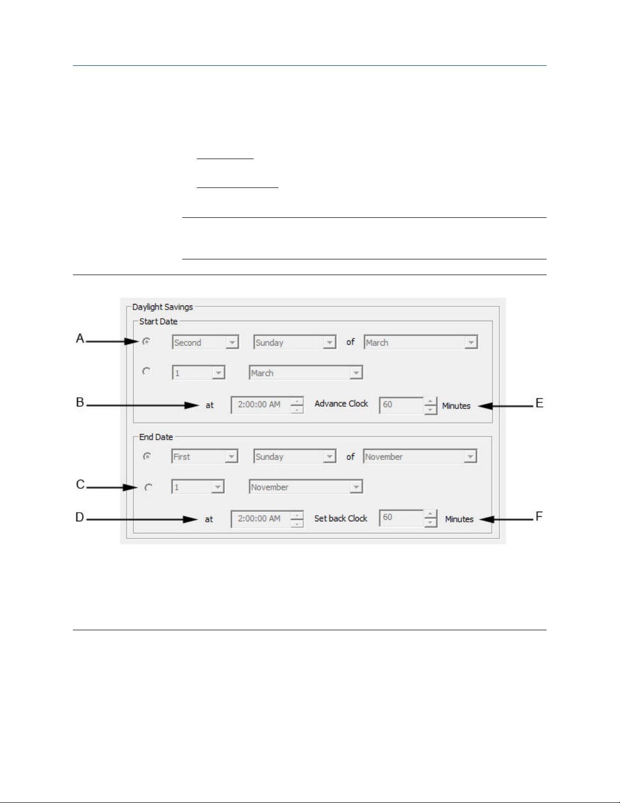
Chromatograph

2. Click the Enable Daylight Savings checkbox.

The Daylight Savings section will be enabled, giving you the following two options for setting the start and end times for daylight savings:

• Week format. You can specify on which week day, of what week, and of what

month DST to start and end.

• Month/Day format. You can specify the exact day of the month and the month

number for which you want daylight savings to start and end.

Note

These formats can be used interchangeably; for example, the Week format can be used to specify the start date, and the Month/Day format can be used to specify the end date.

The Daylight Savings optionsFigure 2-12:

A. Week format B. Start time C. Month/day time D. End time E. Advance time F. Set back time

3. Set the start date for daylight savings time.

4. Set the start time and the advance time.

5. Set the end date for daylight savings time.

6. Set the end time and the setback time.

7. Click OK to implement your changes and close the View/Set Date Time window.

Chromatograph

Note

To implement your changes without closing the View/Set Date Time window, click Save.

Note

Daylight savings time should be configured each time the feature is enabled; thereafter, each year MON2020 will automatically compute the start and end times based on the initial configuration.

Chromatograph

3 Hardware

Many of a gas chromatograph’s hardware components—such as its heaters, valves, and discrete outputs—can be easily managed through MON2020.

This chapter shows you how to view and administer each of a gas chromatograph’s major hardware components.

Hardware

This chapter also shows you how to view an inventory of all of a gas chromatograph’s installed hardware components.

3.1 Heater configuration

MON2020 allows you to do the following from the Heaters window:

• Name each heater.

• Monitor the heaters' performance.

• Set a target temperature.

3.1.1 Set the temperature of the gas chromatograph’s heaters

You can set a heater’s desired temperature or fix its power output by selecting Heaters… from the Hardware menu.

Each heater can be set to one of the following modes:

Auto Allows you to set the desired temperature for the heater.

Fixed On Allows you to set the power output for the heater without regard to

temperature.

Not Used Removes the heater from service.

3.1.2 Rename a heater

To assign an identifying label to a heater, do the following:

1. Select Heaters… from the Hardware menu.

The Heaters window displays.

2. Double-click on the appropriate row under the Label column for the heater that you want to name.

3. Type in a descriptive name for the heater. This name must be unique; two heaters cannot share the same label.

4. Click OK.

Hardware

3.1.3 Set a heater’s voltage type

To set a heater’s voltage type, do the following:

1. Select Heaters… from the Hardware menu.

2. Click on the appropriate Heater Type cell and select AC or DC from the drop-down list.

3. Click OK to save the changes and close the window.

Note

To save the changes without closing the window, click Save.

3.1.4 Monitor the temperature of a heater

To check a heater’s temperature, select Heaters… from the Hardware menu.

The current temperature of each heater displays under the Temperature column, and updates in real time. The percentage of the GC’s power output that is being used by each heater displays under the Current PWM column.

3.1.5 Monitor the operational status of a heater

To check a heater’s status, select Heaters… from the Hardware menu.

The status of each heater displays under the Status column. There are four possible status states, and their meanings are as follows:

OK The heater’s control card is installed and is working correctly.

Not Installed The heater’s control card is not installed.

Out of Control The heater is running and is in the process of reaching its temperature

set point.

Error The GC cannot communicate with the heater.

3.1.6 Set the desired temperature

To set the desired temperature for a heater, do the following:

1. Select Heaters… from the Hardware menu.

The Heaters window displays.

2. For each heater that you want to set, select Auto from the appropriate row under the Switch column.

3. For each heater that you want to set, double-click on the appropriate row under the Setpoint column, and enter the desired temperature, in degrees Celsius. You can enter a value between 20 and 500.

Hardware

Note

Heaters 1 and 2 should never exceed 150 °C.

4. To exclude a heater from the Warm Start process, select its Ignore Warm Start check box.

Note

A warm start occurs when the GC restarts after having been shut down during an auto sequence analysis run. The GC will activate the heaters and wait until they reach their setpoints and the temperature stabilizes; the GC will then resume the auto sequence run.

5. The appropriate rows under the PID Gain, PID Integral, and PID Derivative columns can also be edited by double-clicking and entering a new value. The value ranges for each column is as follows:

PID Gain 0 - 500

PID Integral 0 - 500

PID Derivative 0 - 50000

Note

You should not deviate from the default settings for these variables, which were determined by experienced personnel.

6. Click OK to save the changes and close the window.

Note

To save the changes and leave the window open so that you can monitor the heaters’ status, click Save. The current temperature of each heater displays in the Temperature column, and is updated in real time.

Hardware

3.1.7 Set PWM Output

Note

Pulse-Width Modulation (PWM) is a technique for providing intermediate amounts of electrical power between fully on and fully off.

A heater needs voltage to operate. The amount of voltage that is delivered to a heater can be controlled manually when the heater is set to Fixed On mode. Setting a heater to Fixed On mode can be useful when troubleshooting heater issues.

Hardware

CAUTION!

Fixed On mode is not recommended for general GC operations. Switching a heater to Fixed On mode removes its ability to maintain a constant temperature because the power delivered to the heater will not fluctuate based on the temperature setpoint, but will instead remain at the level set by the user.

To set a heater’s PWM Output, do the following:

1. Select Heaters… from the Hardware menu.

The Heaters window displays.

2. For each heater that you want to set, select Fixed On from the appropriate row under the Switch column.

3. For each heater that you want to set, double-click on the appropriate row under the Fixed PWM Output column, and enter the desired percentage of output. You can enter a decimal value between 0 and 100.

4. Click OK to save the changes and close the window, .

Note

3.1.8 Take a heater out of service

To remove a heater from service, do the following:

1. Select Heaters… from the Hardware menu.

The Heaters window displays.

2. For each heater that you want to set, select Not Used from the appropriate row under the Switch column.

The row turns turquoise, indicating that it is no longer in service.

3. To save the changes and close the window, click OK.

Note

To save the changes without closing the window, click Save.

3.2 Valve configuration

MON2020 allows you to do the following from the Valves window:

• Assign identifying labels to each valve.

• Monitor valve operation.

• Control the operation modes for each valve.

3.2.1 Rename a valve

Hardware

Give each valve a descriptive label to avoid confusing one valve for another. To assign an identifying label, do the following:

1. Select Valves… from the Hardware menu.

The Valves window displays.

2. Double-click on the appropriate row under the Label column for the valve that you want to name.

Note

The valves are labeled Valve 1 - Valve N by default, where N equals the total number of valves available to the GC.

3. Type in a new descriptive name for the valve.

4. Click OK.

3.2.2 Set a valve’s operational mode

A valve has three operational modes: Auto, On, and Off.

• Setting the valve to Off means that the valve will turn off and remain off until the

operational mode is changed.

• Setting the valve to Auto means that the valve will turn on and off according to the

Timed Events table.

• Setting the valve to On means that the valve will turn on and remain on until the

operational mode is changed.

Hardware

Note

The GC’s switch panel or LOI settings override MON2020’s valve settings.

To set a valve’s operational mode, do the following:

1. Select Valves… from the Hardware menu.

The Valves window displays.

2. Select the desired mode from the drop-down menu under the Switch cloumn for the valve.

3. Click OK to save the changes and close the window.

Hardware

Note

To save the changes and leave the window open so that you can monitor the valve’s progress, click Save. The current state of the valve displays in the State column, and is updated in real time.

3.2.3 Monitor the operational status of a valve

To check a valve’s status, select Valves… from the Hardware menu.

The status of each valve displays under the Status column. There are five possible status readings, and their meanings are as follows:

OK The valve is installed and is working correctly.

Not Installed The valve is not installed.

Under/Over Current Error

Error The Heater/Solenoid board is installed but the GC cannot

Unable to switch the solenoid on or off. There is a potential problem with the solenoid.

communicate with it.

3.2.4 Invert the polarity of a valve

The Invert Polarity option reverses the effect of switching a valve on or off. By default, the Invert Polarity option is set to FALSE, which means that switching a valve to ON activates it, and switching the valve to OFF deactivates it. Setting Invert Polarity to TRUE means that switching a valve to ON deactivates it, and switching the valve to OFF activates it.

To set the polarity of a valve, do the following:

1. Select Valves… from the Hardware menu.

The Valves window displays.

2. If the Invert Polarity checkbox is selected, it is set to True; to set it to False, uncheck the box by clicking it. If the Invert Polarity checkbox is not selected, it is set to False; to set it to True, click the box.

3.2.5 Set the usage mode for a valve

A valve’s usage mode determines its general function, or role, during an analysis run. A valve can be assigned one of the following usage modes:

• Unused

• DO (700XA and 1500XA only.)

• FID H2 Valve (700XA and 1500XA only.)

• Common Alarm (700XA and 1500XA only.)

• Stream

• Analyzer01

…

Hardware

• Analyzer016

The usage mode is set at the factory and under ordinary circumstances it should not be changed.

To set the usage mode for a valve, do the following:

1. Select Valves… from the Hardware menu.

The Valves window displays.

2. Select the desired mode from the drop-down menu under the Usage column for the valve.

3. Click OK to save the changes and close the window.

Note

To save the changes and leave the window open so that you can monitor the valve’s progress, click Save. The current state of the valve displays in the State column, and is updated in real time.

3.3 Managing the gas chromatograph's pressure

MON2020 allows you to do the following from the EPC window:

• Change the carrier pressure set point.

• Monitor the EPC's status.

• Switch EPC modes.

Hardware

3.3.1 Change the carrier pressure set point

Note

This feature only works with the 370XA.

1. Select EPC on the Hardware menu.

The EPC window opens.

2. Double-click the Set Point field and enter the desired value.

Note

If the field does not become active after double-clicking it, make sure the Switch field is set to Auto.

3. Click OK.

The new set point will be accepted and the EPC window will close.

Hardware

3.3.2 Check the status of the EPC

Note

This feature only works with the 370XA.

Select EPC on the Hardware menu. The EPC window opens.

Check the Status column to learn the current state of the EPC:

State Description

Ok EPC is working normally and controlling the

Pressure Low The carrier pressure is too low.

Out of range The EPC is not able to control the pressure to

pressure to the set point.

the desired set point.

3.3.3 Switch to a different EPC mode

Note

This feature only works with the 370XA.

1. Select EPC on the Hardware menu.

The EPC window opens.

2. Click the Switch field.

A drop-down listbox opens.

3. Select the appropriate mode.

Option Description

Auto Let's the GC control and maintain its pressure at the desired set point.

Manual Allows you to control the power output for the EPC valve by entering a value, in

the Fixed PWM Output field.

Not Used Shuts off the EPC.

4. Click OK.

The EPC will switch modes and the EPC window will close.

3.4 Detectors

Use the Detectors window to monitor the activity and status of the GC’s detectors.

To view the Detectors window, select Detectors… from the Hardware menu.

Hardware

Note

Before making any modifications to this window, halt the analysis. See Section 6.7 for more information.

Note

Blue cells display read-only data; white cells display editable data.

The following data displays for each detector:

Det # Numerical identifier for the detector to which the following

data applies.

Detector Options, which depend on your GC’s configuration, are TCD,

FPD, or FID.

FID Temp RTD Applies to FIDs only. Select the appropriate RTD from the drop-

down list. The RTD measures the temperature of the FID flame.

FID Ignition Applies to FIDs only. Select Manual if you want to control the

ignition of the FID; select Auto if you want the GC to control the ignition of the FID.

Ignition Attempts Applies to FIDs only. Indicates the number of times the GC will

try to light the flame. If an 'Auto' FID ignition sequence fails to light the flame after the specified number of attempts, the GC will close the hydrogen valve, switch the FID ignition parameter to Manual, and set an active alarm.

Wait Time Bet Tries Applies to FIDs only. Indicates the amount of time, in seconds,

the GC will wait between ignition attempts.

Igniter On Duration Applies to FIDs only. Indicates the length of time that the igniter

will remain on.

Flame On Sense Temp Applies to FIDs only. The flame ignites when the FID internal

temperature exceeds the value set in this field.

Flame Out Sense Temp

FPD Flame Status DI Applies to FPDs only. Allows you to select from a list of available

Preamp Val FID count. Read-only. See Section 3.4.3 for more information.

FID Flame Temp Temperature of the FID flame as read by the RTD. Read-only.

Flame Status Options are: Off, On, and Over Temperature. Read-only.

H2 Valve Cur State Options are: Open and Closed. Read-only.

Scaling Factor Preamp calibration factor.

Applies to FIDs only. The flame is extinguished when the FID internal temperature falls below the value set in this field.

digital inputs. The digital input that is selected will receive the FPD’s flame status value.

Hardware

Igniter Status Options are: Off and On. Read-only.

Electrometer Voltage Output at first stage of FID preamp. Read-only.

Pre Amplifier Voltage Output at second stage of FID preamp. Read-only.

Polarizing Voltage Igniter voltage. Read-only.

FID Gain Status Options are: Low and High.

Status Options are: Ok, Not Installed and Internal Error. Read-only.

3.4.1 Offset the baseline

In some situations that involve TCD detectors the baseline may be displayed either too high on the graph, in which case the tops of the peaks are cut off, or too low on the graph, so that the bases of the peaks are cut off. If this occurs it is possible to offset the baseline either up or down so that the entire peak can be displayed on the graph. This offset will be applied to all traces—live, archived and saved—that are displayed thereafter.

To offset the baseline, do the following:

1. Select Detectors… from the Hardware menu.

The Detectors window displays.

2. Select the appropriate detector. It may be necessary to return to the Chromatogram Viewer to learn which detector is the source of the trace that needs to be offset.

3. To lower the baseline, click Lower Baseline(N). Each time this button is clicked, N is incremented by -1. For example, is this is the first time the button has been clicked, Lower Baseline(0) will be increment to Lower Baseline(-1) and the baseline will be lowered one step. If Raise Baseline(N) was clicked previously, then that button will be incremented by -1 first, until it reached Raise Baseline(0); at the point, Lower Baseline(N) will be incremented by -1.

Note

To reset the baseline to its default setting, click Raise Baseline(N) and Lower Baseline(N) until they read Raise Baseline(0) and Lower Baseline(0).

4. To raise the baseline, click Raise Baseline(N).

5. After the baseline has been raised or lowered to your satisfaction, click OK.

3.4.2 Ignite the FID flame

If the FID Ignition field on the Detectors window is set to “Manual” and if the Flame status field is set to “Off”, do the following to restart the flame:

1. Click Open H2 Valve.

The H2 Valve Cur State field changes to “Open”.

2. Click Ignite.

Hardware

The Flame Status field changes to “On” when the FID internal temperature exceeds the value set in the Flame On Sense Temp field.

Note

If the FID Ignition field is set to “Auto”, the GC will automatically restart the flame if it goes out.

3.4.3 Reset the preamp value

To reset the Preamp Val field on the Detectors window to 0, click Auto-Zero.

3.4.4 Balance the preamp

To offset the baseline, do the following:

1. Select Detectors… from the Hardware menu.

The Detectors window displays.

2. Select the appropriate detector.

It may be necessary to return to the Chromatogram Viewer to learn which detector is the source of the trace that needs to be offset.

3. Balance the preamp:

Hardware

• To lower the baseline, click Left(N). Each time this button is clicked, N is

incremented by -1. For example, is this is the first time the button has been clicked, Left(0) will be increment to Left(-1) and the baseline will be lowered one step. If Right(N) was clicked previously, then that button will be incremented by

-1 first, until it reached Right(0); at the point, Left(N) will be incremented by -1.

Note

To reset the baseline to its original setting, click Right(N) and Left(N) until they read Right(0) and Left(0).

• To raise the baseline, click Right(N). Each time this button is clicked, N is

incremented by 1. For example, is this is the first time the button has been clicked, Right(0) will be increment to Right(1) and the baseline will be raised one step. If Left(N) was clicked previously, then that button will be incremented by 1 first, until it reaches Left(0); at the point, Right(N) will be incremented by 1.

Note

To reset the baseline to its original setting, click Right(N) and Left(N) until they read Right(0) and Left(0).

Hardware

3.5 Discrete inputs

You can use MON2020 to assign labels to the GC’s discrete inputs and to control the discrete inputs’ operational modes. The number of discrete inputs available depends on the GC.

3.5.1 Rename a discrete input

Give each discrete input a descriptive label to avoid confusing one unit for another. To assign an identifying label, do the following:

1. Select Discrete Inputs… from the Hardware menu.

The Discrete Inputs window displays.

2. Double-click on the appropriate row under the Label column for the discrete input that you want to rename.

Note

The discrete inputs are labeled Discrete Input 1 - Discrete Input N by default, where N equals the total number of discrete inputs available to the GC.

3. Type in a new descriptive name for the discrete input.

4. Click OK.

3.5.2 Set a discrete input’s operational mode

A discrete input has three operational modes: Auto, On, and Off.

• Setting the discrete input to Off means that it will interpret all incoming signals as

OFF, despite the true nature of the signal.

• Setting the discrete input to Auto means that it will analyze the incoming signal to

determine whether it is ON or OFF.

• Setting the discrete input to On means that it will interpret all incoming signals as

ON, despite the true nature of the signal.

Note

The GC’s switch panel settings override MON2020’s settings.

To set a discrete input’s operational mode, do the following:

1. Select Discrete Input… from the Hardware menu.

The Discrete Input window displays.

2. Select the desired mode from the drop-down menu under the Switch column for the discrete input.

3. To save the changes and leave the window open so that you can monitor the discrete input’s progress, click Save. The current state of the discrete input displays in the State column, and is updated in real time.

4. To save the changes and close the window, click OK.

Hardware

3.5.3 Monitor the operational status of a discrete input

To check a valve’s status, select Discrete Input… from the Hardware menu.

The status of each discrete input displays under the Status column. There are three possible status readings, and their meanings are as follows:

OK The discrete input is installed and is working correctly.

Not Installed The discrete input is not installed.

Error The Heater/Solenoid board is installed but the GC cannot communicate

with it.

3.5.4 Invert the polarity of a discrete input

The Invert Polarity option reverses the way a voltage signal is interpreted by the discrete input. By default, the Invert Polarity option is set to Normally Open, which means that a low voltage signal is interpreted by the discrete input as ON, and a high voltage signal is interpreted by the discrete input as OFF. Setting Invert Polarity to Normally Closed means that a low voltage signal is interpreted by the discrete input as OFF, and a high voltage signal is interpreted by the discrete input as ON.

To set the polarity of a discrete input, do the following:

1. Select Discrete Input… from the Hardware menu.

Hardware

The Discrete Inputs window displays.

2. Select Normally Open or Normally Closed from the drop-down menu under the Invert Polarity column.

3.6 Discrete outputs

You can use MON2020 to assign labels to the GC’s discrete outputs and to control the discrete outputs’ operational modes. The number of discrete outputs available depends on the GC.

3.6.1 Rename a discrete output

Give each discrete output a descriptive label to avoid confusing one unit for another. To assign an identifying label, do the following:

1. Select Discrete Outputs… from the Hardware menu.

The Discrete Outputs window displays.

Hardware

2. Double-click on the appropriate row under the Label column for the discrete output that you want to rename.

Note

The discrete outputs are labeled Discrete Output 1 - Discrete Output N by default, where N equals the total number of discrete outputs available to the GC.

3. Type in a new descriptive name for the discrete output.

4. Click OK.

3.6.2 Set a discrete output’s operational mode

A discrete output has three operational modes: Auto, On, and Off.

• Setting the discrete output to Off means that the discrete output will turn off and

remain off until the operational mode is changed.

• Setting the discrete output to Auto means that the discrete output will turn on and

off according to the Timed Events table or the Discrete Outputs table.

• Setting the discrete output to On means that the discrete output will turn on and

remain on until the operational mode is changed.

To set a discrete output’s operational mode, do the following:

1. Select Discrete Output… from the Hardware menu.

The Discrete Output window displays.

2. Select the desired mode from the drop-down menu under the Switch cloumn for the discrete output.

3. Click OK to save the changes and close the window.

Note

To save the changes and leave the window open so that you can monitor the discrete output’s progress, click Save. The current state of the discrete output displays in the State column, and is updated in real time.

3.6.3 Monitor the operational status of a discrete output

To check a discrete output’s status, select Discrete Output… from the Hardware menu.

The status of each discrete output displays under the Status column. There are three possible status readings, and their meanings are as follows:

OK The discrete output is installed and is working correctly.

Not Installed The discrete output is not installed.

Error The Heater/Solenoid board is installed but the GC cannot communicate

with it.

3.6.4 Set the usage mode for a discrete output

A discrete output’s usage mode determines which signals are routed to it via the Limited Alarm and Discrete Alarm functions. A discrete output can be assigned one of the following usage modes:

• DO

• Common Alarm

• Stream

• Analyzer01

…

• Analyzer016

• Calibration

• Maintenance

• Calibration or Maintenance

• Validation

• Calibration or Validation or Maintenance

Hardware

To set the usage mode for a discrete output, do the following:

1. Select Discrete Output… from the Hardware menu.

The Discrete Output window displays.

2. Select the desired mode from the drop-down menu under the Usage column for the discrete output.

3. If you select DO for Usage, then you must also set the Start Time and Duration.

a. Click on the appropriate row under the Start Time column and enter the time that

the digital output should be turned on.

b. Click on the appropriate row under the Duration column and enter the amount of

time, in seconds, that the digital output should remain on.

c. Click on the appropriate row under the Interval column and enter the amount of

time, in hours, that should pass before the digital output turns on again.

4. Click OK to save the changes and close the window.

Note

Hardware

3.7 Manage your gas chromatograph’s analog inputs

With MON2020 you can control analog inputs in the following ways:

• Assign identifying labels.

• Assign scale ranges.

• Calibrate analog inputs for zero and full scale values.

Note

Electrical current signals ranging from 4 to 20 mA (±10%) are accepted as analog inputs.

3.7.1 Rename an analog input

Give each analog input a descriptive label to avoid confusing one unit for another. To assign an identifying label, do the following:

1. Select Analog Inputs… from the Hardware menu.

The Analog Inputs window displays.

2. Double-click on the appropriate row under the Label column for the analog input

that you want to rename.

Note

The analog input devices are labeled Analog Input 1 and Analog Input N by default, where N equals the total number of analog inputs available to the GC.

3. Type in a new descriptive name for the analog input.

4. Click OK.

3.7.2 Set an analog input’s operational mode

An analog input has two operational modes: Variable and Fixed.

• Var_Normal: The analog input will be set automatically, based on the signal it

receives. This is the default setting.

• Var_Namur_NE43: Namur_NE43 uses the 3.8 to 20.5 mA signal range for

measurement information, with ≥21 mA or ≤3.6 mA to indicate diagnostic failures.

• Setting the switch to Fixed means that the analog input will be set to the value that

you enter in the appropriate row under the Fixed Value column.

To set an analog input’s operational mode, do the following:

1. Select Analog Input… from the Hardware menu.

The Analog Input window displays.

Hardware

2. Select the desired mode from the drop-down menu under the Switch cloumn for the

analog input.

3. Click OK to save the changes and close the window.

Note

To save the changes and leave the window open so that you can monitor the analog input, click Save. The current value of the analog input signal displays in the Current Value column, and is updated in real time.

Hardware

3.7.3 Set the scale values for an analog input device

To set the zero scale and full scale, which are used when converting the analog input value, do the following:

1. Select Analog Input… from the Hardware menu.

The Analog Input window displays.

2. Double-click on appropriate row under the Zero Scale column and enter a zero scale

value.

3. Double-click on appropriate row under the Full Scale column and enter a full scale

value.

4. Click OK to save the changes and close the window.

Note

To save the changes and leave the window open so that you can monitor the analog input, click Save.

3.7.4 Set the type of analog input signal

The GC’s analog inputs can receive two types of signal: a 0 - 10 V current or the industry standard, which is a 4-20 mA current. To set the type of signal generated by the analog input device, do the following:

1. Select Analog Input… from the Hardware menu.

The Analog Input window displays.

2. Select the signal type from the appropriate row under the mA/Volt column.

3. Click OK to save the changes and close the window.

Note

To save the changes and leave the window open so that you can monitor the analog input’s progress, click Save. The type of signal being generated displays in the mA/Volts column, and is updated in real time.

Hardware

3.7.5 Monitor the status of an analog input

To check an analog input’s status, select Analog Input… from the Hardware menu.

The operational status of each analog input displays under the Status column. There are three possible status readings, and their meanings are as follows:

OK The analog input is installed and is working correctly.

Not Installed The analog input is not installed.

Error The analog input is installed but the GC cannot communicate with it.

This window also displays other types of data, such as the following:

mA/Volts The type of analog input signal being received.

mA If mA displays in the mA/Volts column, then this column displays the amount

of current being received, in milliamperes.

Volts If Volts displays in the mA/Volts column, then this column displays the

amount of current being received, in volts.

Cur Val The current value of the analog input signal.

3.7.6 Calibrate an analog input

To calibrate an analog input, do the following:

1. Select Analog Input… from the Hardware menu.

The Analog Input window displays.

2. Click on the analog input that you want to calibrate.

3. Set the analog input’s Zero Scale by entering its minimum anticipated value.

4. Set the analog input’s Full Scale by entering your maximum anticipated value.

5. Click AutoCal…(F4) or press F4.

The Analog Input Calibration Wizard runs.

6. Click Next.

Step 2 of the Analog Input Calibration Wizard displays.

7. 7. Click Next.

Step 3 of the Analog Input Calibration Wizard displays.

8. 8. Click Next.

Step 4 of the Analog Input Calibration Wizard displays.

9. 9. Click Finish.

The calibration is complete.

3.8 Analog outputs

With MON2020 you can control the analog outputs in the following ways:

• Assign identifying labels.

• Assign scale ranges.

• Calibrate analog outputs for zero and full scale values.

Hardware

3.8.1 Rename an analog output

Give each analog output a descriptive label to avoid confusing one unit for another. To assign an identifying label, do the following:

1. Select Analog Outputs… from the Hardware menu.

The Analog Outputs window displays.

2. Double-click on the appropriate row under the Label column for the analog output

that you want to rename.

Note

The analog output devices are labeled Analog Output 1 - Analog Output N by default, where N equals the total number of analog outputs available to the GC.

3. Type in a new descriptive name for the analog output.

4. Click OK.

3.8.2 Set an analog output’s operational mode

An analog output has two operational modes: Variable and Fixed.

• Setting the switch to Var_Standard means that the analog output will be

proportional to the variable selected in from the Variables column. This is the default setting.

• Var_Namur_NE43: Namur_NE43 uses the 3.8 to 20.5 mA signal range for

measurement information, with ≥21 mA or ≤3.6 mA to indicate diagnostic failures.

• Setting the switch to Fixed means that the analog output will be set to the value

that is entered in the appropriate row under the Fixed Value column.

To set an analog output’s operational mode, do the following:

1. Select Analog Output… from the Hardware menu.

The Analog Output window displays.

2. Select the desired mode from the drop-down menu under the Switch column for the

analog output.

3. Click Save to save the changes and leave the window open so that you can monitor

the analog output.

Hardware

Note

To save the changes and close the window, click OK. The current value of the analog output displays in the Cur Val column, and is updated in real time.

3.8.3 Set the scale values for an analog output device

To set the zero scale and full scale, which are used when converting the analog output value, do the following:

1. Select Analog Output… from the Hardware menu.

The Analog Output window displays.

2. Click on appropriate row under the Zero Scale column and enter a zero scale value.

3. Click on appropriate row under the Full Scale column and enter a full scale value.

4. Click OK to save the changes and close the window.

To save the changes and leave the window open so that you can monitor the analog output’s progress, click Save.

3.8.4 Map a system variable to an analog output

To select the system variable on which to base the signal level of the analog output, do the following:

1. Select Analog Output… from the Hardware menu.

The Analog Output window displays.

2. Select a new variable by clicking on the appropriate drop-down list under the

Variable column.

For a demonstration of how to use the context-sensitive variable selector, see

Section 1.11.

3. Click OK to save the changes and close the window.

Note

To save the changes and leave the window open so that you can monitor the analog output’s progress, click Save.

3.8.5 Monitor the status of an analog output

To check an analog output device’s status, select Analog Output… from the Hardware menu.

The operational status of each analog output displays under the Status column. There are three possible status readings, and their meanings are as follows:

OK The analog output device is installed and is working correctly.

Hardware

Not Installed The analog output device is not installed.

Error The Heater/Solenoid board is installed but the GC cannot communicate

with it.

This window also displays other types of data, such as the following:

mA The amount of current being generated in milliamperes.

Cur Val The current scaled value of the analog output signal.

3.8.6 Calibrate an analog output

To automatically calibrate an analog output, do the following:

1. Select Analog Output… from the Hardware menu.

The Analog Outputs window displays.

2. Click on the analog output that you want to calibrate.

3. Click AutoCal…(F4) or press F4.

The Analog Output Calibration Wizard runs.

4. Select the check box for the unit of measure you want to use for the calibration and

then click Next.

Step 2 of the Analog Output Calibration Wizard displays.

5. Enter the Zero Scale Adjustment value and then click Next.

If the value entered is within tolerance, it is accepted and Step 3 of the Analog Output Calibration Wizard displays. If the value is not within tolerance, an error icon

Hardware

( ) appears beside the field. Tolerance is set to ±1 mA of the analog output’s default zero adjustment setting, which is 4 mA. Enter a different value and try again.

6. Enter the Full Scale Adjustment value and then click Next.

If the value entered is within tolerance, it is accepted and Step 4 of the Analog Output Calibration Wizard displays. If the value is not within tolerance, an error icon

(

) appears beside the field. Tolerance is set to ±1 mA of the analog output’s

default full adjustment setting, which is 20 mA. Enter a different value and try again.

7. Click Finish.

The calibration is complete.

3.9 The Hardware Inventory List

MON2020 can compile an inventory table of all hardware that is installed on the GC. To view this table, select Installed Hardware… from the Hardware menu.

Hardware

The type of hardware installed is listed under the Device Description column. The other types of information available on this screen are the following:

IO Function Describes the function of the device.

Slot Number Describes the location of the hardware in the GC. The slot number refers

to the card cage assembly, which is located in the GC’s lower enclosure and which has eight slots. For the 700XA and 1500XA, the slots are labeled:

• Expansion Slot 1-2

• LOI

• Expansion Slot 1-4

• Base IO

• Foundation Field Bus

There are no slots in the 370XA, therefore this column will display "Analyzer" for all hardware.

Revision The revision number of the backplane.

4 Application

Many of the variables that a gas chromatograph uses during an analysis run—such as timed events, stream sequence, and calculation types—can be easily managed through MON2020.

This chapter explains how to do the following:

• View and edit general information about the GC to which MON2020 is connected,

such as name, model, and default stream sequence.

• View and edit component data, validation data, and timed event tables.

• View and change control, average, and user-defined calculations.

• View and edit limit alarm data.

• View and change stream data.

• View and edit the stream sequence.

• View and edit communication and ethernet port data.

• View and map LOI status variables.

• View and map the FOUNDATION fieldbus process variables.

Application

4.1 Configure the system

To view the System window, select System on the Application menu.

Use this window to select the default GC stream sequence and to set or edit system-wide variables such as the GC’s name, serial number, and system description.

Analyzer Name Defines the GC name that appears in the Status Bar on the main

window when MON2020 is connected to the GC. Can contain up to 12 characters.

System Description A field to record miscellaneous reference information to further

identify the currently connected system. Can contain up to 28 characters.

Site Id Holds customer-defined site identification information.

Company Name The name of the company that operates the GC.

Location The physical location of the GC to which MON2020 is connected.

Model The model number of the GC to which MON2020 is connected.

Serial No Serial number of the GC to which MON2020 is connected.

Firmware Version Revision level of firmware of the GC to which MON2020 is

connected.

Standard Component Table Version for GPA

Indicates which version of the GPA’s standard component table is being used.

Application

Standard Component Table

Indicates which version of the ISO’s standard component table is being used.

Version for ISO

CGM FCAL Archive Sets the storage behavior for final calibration chromatograms. The

options are:

• Keep Last FCAL Per Day - Saves only the last final calibration

chromatogram of the day.

• Keep All FCAL Per Day - Saves all final calibration

chromatograms.

CGM FVAL Archive Sets the storage behavior for final validation chromatograms. The

options are:

• Keep Last FVAL Per Day - Saves only the last final validation

chromatogram of the day.

• Keep All FVAL Per Day - Saves all final validation

chromatograms.

Date Format Defines how the date will be displayed. The options are:

• MM$$DD$$YYYY

• MM$DD$YY

• DD$MM$YYYY

• DD$MM$YY

• YYYY$MM$DD

• YY$MM$DD

$ is the Date Field Separator.

Date Field Separator

Defines the text symbol that will be used as the separator when displaying the date. The options are:

• /

• -

• .

Time Format Defines how the time will be displayed. The options are:

• HH:MM:SS

• HH:MM

Time Notation Defines the cycle of time to use when displaying the time. The

options are:

• 12 Hr

• 24 Hr

Show Advanced System Variables

Allow Multiple

Determines whether advanced system variables will be displayed along with basic system variables.

Determines whether more than one user can connect to the GC.

Writers

Application

Maintenance Mode Switches the GC to maintenance mode and triggers an alarm that

the GC is down for maintenance.

Ideal RF Order/ Limit Check

Applies to the 370XA only. If enabled the GC will verify the following during a calibration:

• The order of magnitude of the response factors for all the

components should be in a particular order. The GC will verify that the response factors follow this pattern.

• The response factor ratio for each component with respect

to a reference component should be within a pre-defined range. The GC will verify that the ratio is within acceptable limits.

Application

Max Warmstart Delay

Applies to the 370XA only. This is the maximum time, after a GC recovers from a power failure during normal operation, that the GC will wait for the heaters and electronic pressure controller to reach their respective set points and stabilize before triggering the Warmstart Failure alarm.

EV Check Applies to the 370XA only. If enabled, the GC analyzes the

calibration gas as an unknown stream and computes its energy value. The GC then compares this value to the Cal Gas Cert CV and determines if the calibration gas' energy value is within the CV Check Allowed Deviation. If it isn't, the GC triggers the Energy Value Invalid alarm.

The following conditions must be met before the GC can perform a EV Check:

• The EV Check flag in the System window must be enabled.

• At least one stream must be set up in the Streams window as

a calibration stream and the Auto flag for this stream must be enabled.

The EV Check is performed under any of the following circumstances:

• During a warm start that follows a power failure during

normal operation. The GC waits for the heater and electronic pressure controller to reach their respective set points and stabilize. It then analyzes the calibration gas as an unknown stream and identifies the peaks. If all the component peaks are identified, the GC computes the calibration gas' energy value and performs the EV Check.

• After a successful calibration, the GC computes the gas'

energy value with the new response factors and performs the EV Check.

GC Sales Serial Number

Calibration Retry on Failure

The sales order number for the GC. When contacting Customer Support, the customer should provide this number to the Customer Support agent.

If a calibration fails, the GC will re-run the calibration sequence.

Application

Calibration Repeatability Check

Metrology Type Shows the metrology type that the GC is configured for.

GC Id

Identification Number

Configuration Checksum at Lockout

Current Configuration Checksum

Checksum Update Time

GC Mode Allows you to select an operating mode for the GC. See Section 1.8 for

Default Stream Sequence

If enabled, the GC will perform a check of the repeatability of calibration runs to the limits specified in ISO6974-1984(E) 8.2.1 Table 6. If the calibration fails to meet the conditions set forth in the table, then the calibration is deemed to have failed and the GC will rerun the calibration sequence.

The checksum of the configuration fields that is calculated when the security switch is locked.

The GC will periodically recalculate and update the configuration checksum. This ‘current’ value will be the latest calculated value.

The time that the configuration checksum was last updated.

more information.

Sets the default sequence to be used by the indicated detector during auto-sequencing. To create a new stream sequence or to edit an

already-created sequence, click Stream Sequence....

See Section 4.10 for more information.

After making changes, click Save to save the changes without closing the window. To save the changes and close the window, click OK.

4.2 The Component Data Tables

MON2020 allows you to view and edit the component data tables. The number of available component data tables depends on the GC unit configuration.

To assign a component data table to a stream, see Section 4.9.2.

1. To view a component data table, select Component Data... from the Application menu.

The Component Data Tables window appears, displaying a list of available component data tables.

Note

Other ways of accessing the component data tables are by pressing F6 or by clicking from the Toolbar.

2. Select the table that you want to view.

The selected component data table displays.

Note

To see a different table, select it from the Choose table drown-down list.

Note

To sort the list of components by detector, and then by retention time, click Sort RT.

Application

4.2.1 Edit a Component Data Table

Note

Table cells with a white background are editable; table cells with a turquoise background are not editable.

To edit a cell, do the following:

1. Click on the cell.

Depending on the cell type, you will either be required to select a value from a dropdown list, or you will be able to type in the value directly.

2. To save the changes and close the window, click OK.

Note

To save the changes without closing the window, click Save.

The following table lists all of the editable parameters available on the Component Data Table window. The standard values for these parameters were taken from the second editions of the Orifice Metering of Natural Gas and Other Related Hydrocarbon

Fluids and the Compressibility Factors of Natural Gas and Other Related Hydrocarbon Gases.

Application

Component This drop-down list contains the complete catalog of

available components for the selected stream.

Usr Std Indicates the source of the component:

• Usr - The component was edited or defined by the user.

• Std - The component was selected from the standard list

of components and no changes were made to its standard data.

Det # The component’s detector number.

Ret Time Time in seconds before the apex of the component’s peak will

appear. The rentention time can be set from 0 to 3600 seconds.

Application

CAUTION!

Ensure that the component retention times do not exceed the analysis time, as defined by the Timed Events table. MON2020 does not automatically prevent the user from defining excessive component retention times.

Resp Fact A component’s response factor is equal to the raw data of the

component’s peak divided by the component’s concentration. The maximum value is 1.0E+38.

Calib Type MON2020 can perform four types of calibrations:

• Single-Level - Uses the standard calibration in which the

response factor is needed to determine the mole percentage during the calibration.

• Fixed - During the calibration, the response factor is not

updated.

• Relative - Calibration in which a reference component is

used to compute the mole percentage.

• Multi-Level - Uses a polynomial equation to compute the

mole percentage during the calibration. Values must be entered in the Mult-level Calib ‘a’, Mult-level Calib ‘b’, Mult-level Calib ‘c’, and Mult-level Calib ‘d’ cells.

Calib Conc The amount, in mole percent, parts per million (ppm) or parts

per billion (ppb), of the component that is present in the calibration gas.

Unit Indicates the unit of measure used when calculating and

displaying the component’s calibration concentration. Options are Mole%, ppm and ppb.

Anly Meth Defines how the component concentration is computed. The

analysis method can take one of the following values:

• Area - Calculates the component concentration by

dividing the peak area by the response factor.

• Height - Calculates the component concentration by

dividing the peak height by the response factor.

• Fixed - The component concentration equals the

component's calibration concentration displayed in the Calib Conc column of the component data table. No calculation is performed using the response factor.

• Analog Input - The GC reads the analog input channel,

scales the raw milliampere value to engineering values that were set in the Analog Inputs window, and uses this value as the component concentration. No calculation is performed using the response factor.

RT Secs Dev The maximum acceptable deviation time, in seconds, of the

new retention time from the current retention time.

Application

RT Upd Meth Determines when the retention time will be updated. Options

are:

• Cal - Updates the retention time only during the final

calibration run.

• Anly - Updates after each analysis.

Resp Fact % The maximum acceptable percent of deviation between the

new response factor and the current response factor.

Gross Dry BTU Gross energy content per cubic foot (ft3), assuming no water

is present.

Net Dry BTU Net energy content per cubic foot, assuming no water is

present.

Gross Dry BTU perlbGross energy content per pound, assuming no water is

present.

HV Sup MJ/m

HV Inf MJ/m

Gross heating value in megajoules per cubic meter.

Net heating value in megajoules per cubic meter.

HV Sup MJ/kg Gross heating value in megajoules per kilogram.

HV Inf MJ/kg Net heating value in megajoules per kilogram.

Sum Factor Pri Used to calculate the compressibility factor.

Sum Factor Sec Used to calculate the compressibility factor.

CV Superior Pri Gross caloric value per kilojoule (kJ).

CV Inferior Pri Net caloric value per kilojoule (kJ).

CV Superior Sec Gross caloric value per kilojoule (kJ).

CV Inferior Sec Net caloric value per kilojoule (kJ).

Gals/1000 SCF Liquid equivalent volume in gallons/1000ft3.

Reid Vapor The component’s vapor pressure in pounds per square inch

(psia) at 100.0 °F

LBs/Gallon Liquid density for the component at base conditions.

Rel Dens Gas The relative density of the gas phase for the component at

base conditions.

Rel Dens Liquid The relative density of the liquid phase for the component at

base conditions.

Molecular Weight The molecular weight of the component, which is used to

calculate the weight percent of each component in the sample.

Carbon Weight The molecular weight of the carbon atoms in the component.

AGA 8 Component

The name of the component according to the American Gas Association, which is used in the AGA 8 compressibility calculation.

Ref Comp The component not found in the calibration gas but in the

sample gas for indirect calibration. If ‘none’, normal (direct) calibration is used.

Not editable unless the calibration type is set to Relative.

Application

Rel Resp Fact A fixed multiple of the response factor of the component

found in the sample gas for indirect calibration. Not editable unless the calibration type is set to Relative.

Rel Dens Liquid 15C

The relative density in kilograms per cubic meter (kg/m3) of the liquid phase for the component at 15 °C.

Molar Mass The mass of one mole of the component.

Mult-level Calib ‘a’

Mult-level Calib ‘b’

Third-order polynomial coefficient for multi-level calibrations. Not editable unless the calibration type is set to Multi-Level.

Second-order polynomial coefficient for multi-level calibrations.

Not editable unless the calibration type is set to Multi-Level.

Mult-level Calib ‘c’

Mult-level Calib ‘d’

First-order polynomial coefficient for multi-level calibrations. Not editable unless the calibration type is set to Multi-Level.

Zero-order polynomial coefficient for multi-level calibrations. Not editable unless the calibration type is set to Multi-Level.

Component Code An index number that corresponds to the standard

component numbers taken from the American Gas Association. Up to 20 components can be defined per data table.

4.2.2 Add a component to a Component Data Table

To add a component to a component data table, do the following:

1. Select Component Data... from the Application menu.

The Component Data Tables window appears, displaying a list of available component data tables.

Note

Other ways of accessing the component data tables are by pressing F6 or by clicking from the Toolbar.

2. Select the table that you want to view.

The selected component data table displays.

Note

To sort the list of components by detector, and then by retention time, click Sort RT.

3. If you want to add the component above the currently selected component, click Insert before. If you want to add the component below the currently selected component, select Insert after from the Insert arrow.

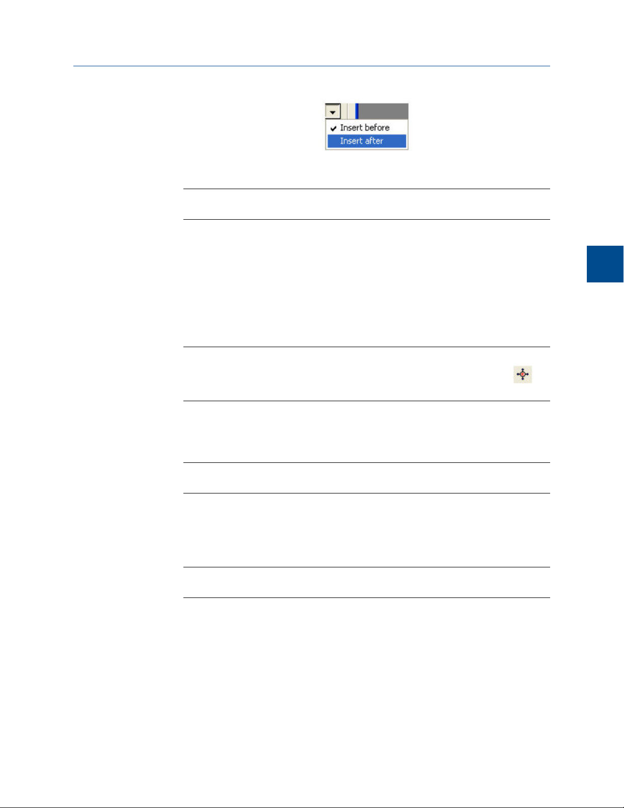
Application

4. To save the changes and close the window, click OK.

Note

To save the changes without closing the window, click Save.

4.2.3 Remove a component from a Component Data Table

Application

To remove a component from a component data table, do the following:

1. Select Component Data... from the Application menu.

The Component Data Tables window appears, displaying a list of available component data tables.

Note

Other ways of accessing the component data tables are by pressing F6 or by clicking from the Toolbar.

2. Select the table that you want to view.

The selected component data table displays.

Note

To sort the list of components by detector, and then by retention time, click Sort RT.

3. Select the component that you want to remove.

4. Click Delete.

5. To save the changes and close the window, click OK.

Note

To save the changes without closing the window, click Save.

4.2.4 View the standard values for a component

If a component’s values have been changed by the user, it is still possible to view the standard values for that particular component. To view the standard values for a component, do the following:

1. Select Component Data... from the Application menu.

The Component Data Tables window appears, displaying a list of available component data tables.

Application

Note

Other ways of accessing the component data tables are by pressing F6 or by clicking from the Toolbar.

2. Select the table that you want to view.

The selected component data table displays.

Note

To sort the list of components by detector, and then by retention time, click Sort RT.

3. Click Std Values (F3).

The Standard Component Values window displays.

4. When you are finished viewing the window, click Close.

4.2.5 Display raw data from the Component Data table

To view the raw data for the displayed component data table, do the following:

1. Select Component Data... from the Application menu.

The Component Data window displays.

2. Click Raw Data (F4) or press F4.

The Select dialog displays, listing the streams that are associated with the component data table.

3. Double-click the desired stream.

The Raw Data window appears, listing the peak raw data from the last run of the stream represented by the component data table.

The following data displays for each peak:

Peak No. Numerical identifier for the peak, listed by the order of

discovery.

Ret Time Time, in seconds, that the component eluted.

Peak Area The area under the peak.

Peak Height The maximum height of the peak.

Det The detector associated with the peak.

Method Method of peak end detection. Options are:

• 1 (Baseline). Baseline termination occurs when the absolute

values of twelve successive slope calculations are less than the slope sensitivity.

Application

• 2 (Fused Peak). A fused peak is found if a peak onset is

detected subsequent to the discovery of a peak crest and before the baseline termination is detected.

• 3 (Last Fused Peak). The last peak in a group of fused peaks.

• 4 (Tangent Skim). Baseline termination occurs when the

current level is lower than the Start Baseline value and the slope at the point is negative and smaller in magnitude than the average slope from the beginning of the peak.

• 100 (Inhibit). An Inhibit On event in the Timed Events table

caused the peak to be terminated.

• 300 (Forced Integration). An Integration Off event in the

Timed Events table caused the peak to be terminated.

• 500 (Summation). A Summation Off event in the Timed

Events table caused the peak detection logic to sum together the peak areas under multiple peaks between the Summation On and Summation Off events and to add an entry for an artificial peak with its area set to the composite area under the constituent peaks.

Application

Baseline Start The raw detector counts at the start of an integration. For

example, if the peak starts at 10 seconds, then the raw detector counts at 10 seconds becomes the Baseline Start value.

Baseline End The raw detector counts at the end of an integration. For

example, if the peak ends at 35 seconds, then the raw detector counts at 35 seconds becomes the Baseline End value.

Integration Start

Integration Stop

Peak Width @ Half Height

Partial Peak If Yes, then the Partial Peak value is used in the summation

4. Click Close to return to the Component Data window.

Time, in seconds, when integration started.

Time, in seconds, when integration stopped.

The width of the peak taken at half of the peak’s height.

calculation; if No, then the Partial Peak value is not used in the summation calculation.

4.2.6 Change the default C6+ mixture ratio

The C6+ component that is detected by the GC is actually a mixture of up to four heavy hydrocarbons -- from hexane and above. When the energy value and other physical properties are calculated for the mixture, the GC assumes a ratio of heavy hydrocarbon components is used for the C6+ value. By default, there are four pre-defined ratios:

Component C6/C7/C8 percentages

C6+ 47/35/17 47.466/35.34/17.194

Application

Component C6/C7/C8 percentages

C6+ GPA 2261-99 60.0/30.0/10.0

C6+ 57/28/14 57.143/28.572/14.285

C6+ 50/50/0 50.0/50.0/0

To define a different ratio, do the following:

1. Select Component Data on the Application menu.

The Component Data window opens.

Note

You can also click F6 to open the Component Data window.

2. Click the first field in the Component column. This is the C6+ component field and it will display one of the four ratios described above.

A drop-down list opens.

3. Select C6+ (User Def.) from the drop-down list.

4. Click Edit Percentage.

The C6+ User Def. window opens.

5. Enter a composition percentage for each component.

The Total Percentage, which must equal 100 and is displayed on the window's title bar, will update with the sum of the four ratios.

6. Click OK.

The Component Data window closes. The C6+ row on the Component Data table will be updated based on the new ratio.

7. Click Save to accept the changes without closing the window; click OK to accept the changes and to close the window.

4.3 The Timed Events tables

Use this function to view and/or edit the timed events tables assigned to and used by particular gas streams. The number of available timed events depends on the GC unit configuration. The standard GC application contains four timed events tables.

Note

See Section 2.5.2 for more information about editing timed events from the Chromatogram Viewer. To assign a timed events table to a stream, see Section 4.9.2.

Application

1. Select Timed Events... from the Application menu. The Timed Events Tables selector window appears, displaying a list of available timed events tables.

Note

Other ways of accessing the timed event tables are by pressing F5 or by clicking from the Toolbar.

Note

If only one timed events table is available, it will display immediately, bypassing the Timed Events Tables selector window.

2. Select the table that you want to view.

The selected timed events table displays.

Note

To sort events by time, click the appropriate Sort button.

3. To see a different timed events table, select it from the Choose table drop-down list.

4.3.1 Configure valve events

Valve-related events are grouped on the upper left side of the Timed Events window. To edit valve-related events, do the following:

1. Select Timed Events... from the Application menu.

The Timed Events Tables selector window appears, displaying a list of available timed events tables.

Note

Application

Other ways of accessing the timed event tables are by pressing F5 or by clicking the Toolbar.

Note

If only one timed events table is available, it will display immediately, bypassing the Timed Events Tables selector window.

2. Select the table that you want to view.

The selected timed events table displays.

Note

To sort events by time, click the appropriate Sort button.

3. Click on the cell that you want to edit.

from

Application

Depending on the cell type, you will either be required to select a value from a dropdown list, or you will be able to type in the value directly. The following list describes the valve-related parameters that are available on the Timed Events window.

TEV Type The type of device associated with the event. You have the following

choices:

• Valve #

• DO # - A discrete output.

• Strm Sw - Switches to the next stream in the sequence.

• Cal Gas Save - Sets the start or end time for the Cal-Gas Saver

feature.

Valve/ DO #

Use the drop-down menu to select the specific valve or discrete output that should be used for the event.

This column does not apply if Strm Sw was selected from the TEV Type column.

State Turns the valve or discrete output on or off, or sets the FID to high or

low. This column does not apply if Strm Sw was selected from the TEV Type

column.

Time Indicates the time, in seconds, that the event should occur during the

analysis. Enter a value between 0.0 and 3600.0.

Note

Event times must be less than the analysis time.

4. To save the changes and close the window, click

Note

To save the changes without closing the window, click Save.

4.3.2 Configure integration events

OK.

Integration-related events are grouped on the upper right side of the Timed Events window. To edit integration-related events, do the following:

1. Select Timed Events... from the Application menu.

The Timed Events Tables selector window appears, displaying a list of available timed events tables.

Note

Other ways of accessing the timed event tables are by pressing F5 or by clicking the Toolbar.

from

Note

If only one timed events table is available, it will display immediately, bypassing the Timed Events Tables selector window.

2. Select the table that you want to view.

The selected timed events table displays.

Note

To sort events by time, click the appropriate Sort button.

3. Double-click on the cell that you want to edit.

Depending on the cell type, you will either be required to select a value from a dropdown list, or you will be able to type in the value directly. The following list describes the integration-related parameters that are available on the timed events window.

Application

TEV Type

The type of integration event. You have the following options:

• Inhibit: Set to Off to start look for a peak; set to On to stop looking for

a peak.

• Integrate: Set to On and Off to set a region in which the area under

the trace is computed as a peak regardless of peak onset discovery. The resulting area is added to the raw data as a peak with the retention time set to the Integration Off time.

• Summation: Set to On and Off to set a region in which the area of all

peaks found will be added together to create a single summed value. The peaks that contribute to the summation are marked as partial peaks in the raw data table, and the summation total is added to the raw data as a new peak with the retention time set to the Summation OFF time.

• Slope Sens: The peak starts when the slope of six consecutive points is

greater than the slope sensitivity value that is displayed in the Value column; the peak ends when the slope of six consecutive points is less than the slope sensitivity value that is displayed in the Value column.

• Peak Width: Each point displayed on the graph represents the

average of N raw data points, where N is the value displayed in the corresponding Value column.

• Single Base: Determines how the baseline is drawn under a peak.

- Off: The baseline is drawn from the point of peak onset to the

point of peak termination. This is not necessarily horizontal and if fact usually has a slight slope. (Default)

- Bgn: Draws a horizontal baseline from the point of peak onset to a

point above or below the peak termination.

- End: Draws a horizontal baseline from a point above or below the

peak onset to the point of peak termination.

• Fused Ovrrd: Determines how the baseline is drawn when two or

more peaks are ‘fused’ together.

Application

- Off: A single baseline is drawn from the onset of the first peak of

the fused group to the termination of the last peak of the group. (Default)

- On: Causes a separate baseline to be drawn for each peak in the

fused group.

• Negative Peak: Determines whether peak detection will detect

inverted peaks, which are peaks that point downward from the baseline. At any given moment we can detect positive or negative peaks but not both at once.

- Off: Detect positive peaks. (Default)

- On: Detective negative peaks.

TEV Type

SW Auto Zero: Re-zeros the baseline of the trace at the specified time for the specified detector. Used after a FID gain change event or a spectrum gain change event.

Note

The Single Base and Fused Override events can act together to produce multiple horizontal baselines, at different heights, for a fused peak group.

Value The values available depend on the integration type selected from the

TEV Type column.

• Slope Sensitivity and Peak Width: Enter the number of points,

between 1 and 99, to be used.

• Single Baseline: Select Off, End, Bgn.

• SW Auto Zero: No options.

• All other integration types: Select On or Off.

Det # The ID number of the detector that will be affected by the event. Valid

values are 1 and 2.

Time Indicates the time, in seconds, that the event should occur during the

analysis. Enter a value between 0.0 and 3600.0.

Note

Event times must be less than the analysis time.

4. To save the changes and close the window, click OK.

Note

To save the changes without closing the window, click Save.

4.3.3 Configure spectrum gain events

The spectrum gain feature graphically magnifies the size of a chromatogram’s peaks. The data itself is not affected; only the presentation of the data. This feature can be useful for viewing peaks that are otherwise too small to examine or so large that the top of the peak can not be seen.

Spectrum gain-related events are grouped on the lower left side of the Timed Events window. To edit spectrum gain-related events, do the following:

Application

1. Select Timed Events... from the Application menu.

The Timed Events Tables selector window appears, displaying a list of available timed events tables.

Note

Other ways of accessing the timed event tables are by pressing F5 or by clicking from the Toolbar.

Note

If only one timed events table is available, it will display immediately, bypassing the Timed Events Tables selector window.

2. Select the table that you want to view.

The selected timed events table displays.

Note

To sort events by time, click the appropriate Sort button.

3. Click on the cell that you want to edit.

Application

Depending on the cell type, you will either be required to select a value from a dropdown list, or you will be able to type in the value directly. The following list describes the spectrum gain-related parameters that are available on the timed events window.

Det # The ID number of the detector that will be affected by the event. Select 1 or

Gain Enter a value between 0 and 64. This is the exponent value in the following

expression: 2

gain value

. For example, a value of 0 means no gain is applied; a

value of 5 means the gain is increased to 32 times it’s original value.

Time Indicates the time, in seconds, that the event should occur during the

analysis. Enter a value between 0.0 and 3600.0.

Note

Event times must be less than the analysis time.

Application

4. To save the changes and close the window, click OK.

Note

To save the changes without closing the window, click Save.

4.3.4 Set the cycle and analysis time

To set the cycle and analysis time, do the following:

1. Select Timed Events... from the Application menu.

The Timed Events Tables selector window appears, displaying a list of available timed events tables.

Note

Other ways of accessing the timed event tables are by pressing F5 or by clicking from the Toolbar.

Note

If only one timed events table is available, it will display immediately, bypassing the Timed Evetns Tables selector window.

2. Select the table that you want to view. The selected timed events table displays.

The Analysis Time section is located on the lower right side of the Timed Events window.

Note

To sort events by time, click the appropriate Sort button.

3. Click on the Analysis Time cell and enter a value, in seconds, between 0 and 3600.

4. Click on the Cycle Time cell and enter a value, in seconds, between 0 and 3620.

Note

The Cycle Time must be at least 10 seconds greater than the Analysis Time.

5. To save the changes and close the window, click OK.

Note

To save the changes without closing the window, click Save.

4.3.5 Remove an event from the Timed Event Table

To remove an event from one of the Valve Events, Integrate Events, or Spectrum Gain Events tables on the Timed Events window, do the following:

1. Select Timed Events... from the Application menu.

The Timed Events Tables selector window appears, displaying a list of available timed events tables.

Note

Other ways of accessing the timed event tables are by pressing F5 or by clicking from the Toolbar.

Note

If only one timed events table is available, it will display immediately, bypassing the Timed Events Tables selector window.

2. Select the table that you want to view.

The selected timed events table displays.

Note

To sort events by time, click the appropriate Sort button.

Application

3. Select the event that you want to delete.

4. Click the appropriate Delete button.

4.3.6 Add an event to the Timed Event Table

To add an event to one of the Valve Events, Integrate Events, or Spectrum Gain Events tables on the Timed Events window, do the following:

1. Select Timed Events... from the Application menu.

The Timed Events Tables selector window appears, displaying a list of available timed events tables.

Note

Other ways of accessing the timed event tables are by pressing F5 or by clicking the Toolbar.

Note

If only one timed events table is available, it will display immediately, bypassing the Timed Events Tables selector window.

2. Select the table that you want to view.

from

The selected timed events table displays.

Application

Note

To sort events by time, click the appropriate Sort button.

3. If you want to add the event above the currently selected event, click the appropriate Insert before button. If you want to add the event below the currently selected event, select Insert after from the Insert arrow and then click the button.

The new event will be added to the table.

4. Select a Type, Valve/DO#, and State for the event, if necessary, and enter a new Time for the event also.

5. To save the changes and close the window, click OK.

Note

To save the changes without closing the window, click Save.

4.4 The Validation Data Tables

Use the validation data table to hold information about the composition of the gas that is used in the validation run. During a validation run, the GC performs a test analysis of a gas with a known component composition to verify that the GC is working properly.

To add a component to the validation data table, do the following:

1. Select Validation Data from the Application menu.

The Validation Data window displays.

2. If the appropriate table is not displayed, select it from the Choose Table drop-down list.

3. Select a new variable by clicking on the appropriate drop-down list under the Variable column.

For a demonstration of how to use the context-sensitive variable selector, see

Section 1.11.

4. Enter the component’s concentration percentage in the appropriate cell under the Nominal Value column.

To ensure accuracy, this value, which is compared to the GC’s analysis results at the end of the validation run, should be taken from the documentation provided with the gas cylinder.

5. Enter a value in the appropriate Percent Deviation cell.

Example: If you enter 10 in this field, and the GC’s analysis result for the component differs from the component’s Nominal Value by ±10% or more, then an alarm is generated.

6. To copy a component variable to the next empty row, click C + Copy.

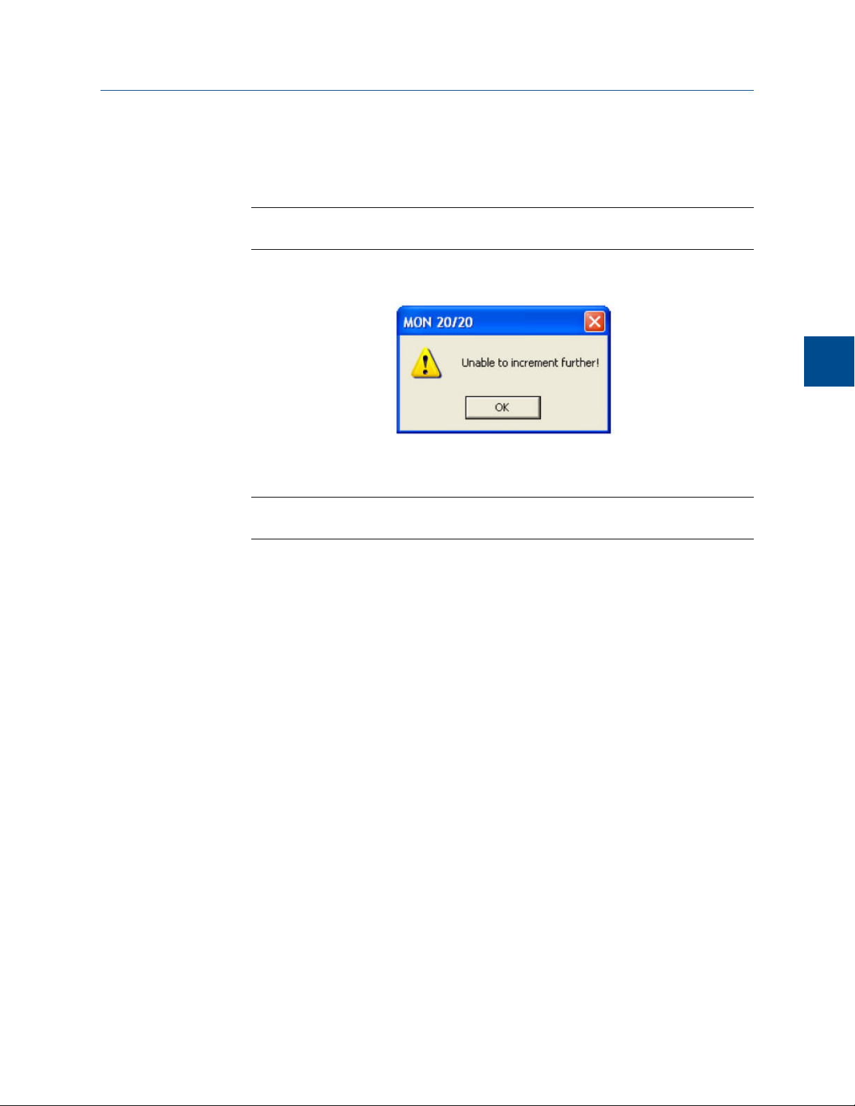
The component will be increment to the next available component—for example, from Ammonia to Benzene. The Nominal Value and Percent Deviation values will also be copied.

Note

You can select and copy more than one component at a time.

If there are no components available, instead of copying the component, MON2020 will display the following message:

7. To save the changes and close the window, click OK.

Application

Note

To save the changes without closing the window, click Save.

4.5 Calculations

MON2020’s Calculations submenu allows you to activate and define how the output of standard or user-defined chromatograph analysis data is used in various calculations.

You can configure the following types of calculations:

• Control - Allows you to designate, by streams, the standard calculations that should

be performed from the analysis data.

• Averages - Allows you to designate, by streams and components, averages of

standard calculations MON2020 should perform.

• User Defined - Allows you to create and edit customized calculations using analysis

data. See Appendix A for more information.

• Dewpoint - This optional feature allows you to calculate dewpoint temperatures

and to estimate the cricondentherm, which is the temperature above which no liquid will form at any pressure.

4.5.1 Set standard calculations by stream

To designate, by streams, the standard calculations—for example, mole percent, liquid volume, gas density, Wobbe index, etc.—that should be performed from the analysis data, do the following:

1. Select Applications → Calculations → Control....

Application

The Control Calculations window appears.

2. Select a check box for a given stream to turn the calculation ON for that stream; click to clear the check box for a given stream to turn the calculation OFF for that stream.

You can use the arrow keys to move from one stream cell to another, and you can press the space bar to toggle the calculation on or off.

3. To save the changes and close the window, click OK.

Note

To save the changes without closing the window, click Save.

Note

To save the information on this screen to a tab-delimited text file, right-click on the table and select Save Sheet from the right-click menu.

Note

To copy the information on this screen to the clipboard so that it can be pasted into another application such Microsoft Word or Excel, right-click on the table and select Copy to clipboard from the right-click menu.

Note

To print the information on this screen, right-click on the table and select Print Sheet from the right-click menu.

4.5.2 Edit average calculations

To designate, by streams and components, averages of standard calculations the GC should perform, do the following:

1. Select Applications → Calculations → Averages....

The Averages Calculations window appears.

2. Select a new variable by clicking on the appropriate drop-down list under the Variable column.

For a demonstration of how to use the context-sensitive variable selector, see

Section 1.11.

Note

The averages will be assigned in the default Modbus map in the order that they appear in the table.

3. Select the type of average to be calculated from the Average Type drop-down list. You have the following options:

Unused An average will not be calculated for the variable.

Emerson MON2020 User Manual

Specifications and Main Features

Frequently Asked Questions

User Manual

NOTICE

Warranty

Contents

Getting started

1.1 MON2000 and MON2020

1.2 Getting started with MON2020

1.2.1 System requirements

1.2.2 Install MON2020

1.2.3 Start MON2020

1.2.4 Register MON2020

1.2.5 Set up the data folder

1.2.6 Set up MON2020 to connect to a gas chromatograph

1.2.7 Export a GC directory

1.2.8 Import a GC Directory file

1.2.9 Launch MON2020 from the SNAP-ON for DeltaV

1.2.10 Launch MON2020 from the AMS Device Manager

1.2.11 The MON2020 user interface

The main user interface

The GC Status Bar

1.2.12 Connect to a gas chromatograph

1.2.13 Disconnect from a gas chromatograph

1.3 Keyboard commands

1.4 Procedures guide

1.5 Configuration files

1.5.1 Edit a configuration file

1.5.2 Save the current configuration

1.5.3 Import a configuration file

1.5.4 Restore the GC's factory settings

1.6 Configure your printer

1.7 Online help

Operating Modes for MON2020Table 1-2:

1.9 The Physical Name column

1.10 Select the GC’s networking protocol

1.11 The context-sensitive variable selector

Chromatograph

2.1 The Chromatogram Viewer

2.1.1 Data displayed in the chromatogram window

2.1.2 Display a live chromatogram

2.1.3 Display an archived chromatogram

2.1.4 Protected chromatograms

2.1.5 Display a saved chromatogram

2.2 Options for displaying chromatograms

2.3 Configure the appearance of the chromatograph

2.3.1 The Graph bar

2.3.2 Additional plot commands

2.4 Change how a chromatogram displays

2.4.1 Edit a chromatogram

2.4.2 Display chromatogram results

2.4.3 Save a chromatogram

2.4.5 Initiate a forced calibration

2.4.6 Chromatogram Viewer tables

2.4.7 Open a comparison file

2.4.8 Save a comparison file

2.5 Miscellaneous commands

2.5.1 The Chromatogram Viewer's Timed Events table

2.5.2 Launch the Timed Events table from the Chromatogram Viewer

2.5.3 Edit Timed Events from the Chromatogram Viewer

2.5.4 Use the Chromatogram Viewer’s cursor to update a Timed Event

2.5.5 The Chromatogram Viewer's Component Data table

2.5.6 Edit retention times from the Chromatogram Viewer

2.5.7 Display raw data from the Chromatogram Viewer

2.6 Set the gas chromatograph’s date and time

2.6.1 Set daylight savings

Hardware

3.1 Heater configuration

3.1.1 Set the temperature of the gas chromatograph’s heaters

3.1.2 Rename a heater

3.1.3 Set a heater’s voltage type

3.1.4 Monitor the temperature of a heater

3.1.5 Monitor the operational status of a heater

3.1.6 Set the desired temperature

3.1.7 Set PWM Output

3.1.8 Take a heater out of service

3.2 Valve configuration

3.2.1 Rename a valve

3.2.2 Set a valve’s operational mode