Dxo OPTICS PRO V4.2 User Manual

Download

Page 1

DxO Optics Pro V4.2 Reference Manual

DxO Optics Pro V4.2

Reference Manual

Page 2

DxO Optics Pro V4.2 Reference Manual

Contents

Introduction 4 Introducing DxO Optics Pro V4

Chapter 1 6 A typical image enhancement session from A to Z

Selecting images to create a project Organizing your project Enhancing the images in your project Processing a batch of images Viewing the results! Common actions Note for users of previous versions

Chapter 2 9 Select your photos from various sources

The thumbnails and their buttons

Star-ranking Adding images Fully automatic operation

Chapter 3 12 Organize your images on an electronic light-table

The big picture

Adapt your workspace

Chapter 4 14 Enhance your images using DxO Optics Pro Tools Corrections Palette

Guided or Expert? Eight corrections palettes

Chapter 5 18 Process as many images as you want with just

one click

Process the stars Define output formats

Chapter 6 20 View the results of your work (with a little help from DxO)

Chapter 7 21 How to go further

Your workflow

Page 3

DxO Optics Pro V4.2 Reference Manual

Chapter 8 22 DxO Optics Pro Menus

Chapter 9 28 Using Auto, Guided and Expert modes

Chapter 10 31 Generic Tools

Chapter 11 34 DxO Optics Tools

Chapter 12 40 Sharpness Tools

Chapter 13 43 DxO Noise Tools

Chapter 14 45 White Balance and Exposure

Chapter 15 49 DxO Color Tools

Chapter 16 55 DxO Lighting Tools

Chapter 17 58 Geometry Tools

Chapter 18 63 Stacking, ranking and Output Formats

Chapter 19 67 DxO Optics Pro for Photoshop

Copyrights, Trademarks and Registered marks are properties of their respective owners, which may include, but are not limited to, Nikon, Canon, Kodak, Fuji, Sony and others.

Page 4

DxO Optics Pro V4.2 Reference Manual

Introduction

Welcome to the exciting world of DxO Optics Pro digital image enhancement!

This powerful, groundbreaking software is going to improve the quality of your digital images in a way you would never have believed possible.

DxO Optics Pro’s precise, calibrated corrections are based on unique algorithms derived from actual measurements made on real camera bodies and lenses. Thousands of test measurements are made on each body and lens combination, with every permutation of shooting parameters.

This is why the whole DxO Optics Pro system operates using what are called ‘Correction Modules’, each unique and specific to a particular body / lens combination; for this reason, you need to make sure you have the right module(s) for the bodies and/or lenses you use. All this means that DxO Optics Pro produces extremely accurate actual corrections of measured phenomena, instead of just subjective (and often impossibly time-consuming) manual approximations.

In addition, this new version 4 of the software also includes a number of corrections that are not camera-specific, so you can make the most of other images too, and some adjustments, going beyond purely correction, that you can perform manually for creative effect.

A simple workflow

The way the DxO Optics Pro workflow is organized is perhaps worth explaining briefly. You start by creating a new ‘project’, which you can name and save, and into which you will assemble the pictures you wish to process at this time. You can then click on the “Process Now” button to start processing the images with DxO automatic presets. Alternatively, you can work on preview images to define your own corrections or adjustments.

And it’s worth underlining that your original image files are left untouched, they are never altered in any way, deleted, or overwritten, so your precious originals are 100% safe at all times!

What makes DxO Optics Pro even more powerful and ergonomic, is that some or all of your chosen settings can be saved as one or more ‘presets’ that can be applied across a whole series of images — but still leaving you the possibility of making further manual adjustments too, of course! Even without the use of any manual settings at all, DxO Optics Pro can process your images fully automatically, for guaranteed improved results every time!

Page 5

DxO Optics Pro V4.2 Reference Manual

You choose between three different working modes: “Auto” is the most straightforward, since you will only use the automatic enhancement settings provided by DxO Optics Pro. “Guided” gives you access to the Enhancement tab, where you can decide which global setting (as “Portrait”, “Landscape”, etc) to use; and “Expert” gives you the possibility of overriding every option of all the corrections performed by DxO Optics Pro. The choice you made at the first launch of the software can be changed anytime in Preferences (Edit Menu).

Upfront in your workflow!

DxO Optics Pro is designed to be at the very beginning of the workflow, at the point images are copied from the card reader or camera, to correct images straight out of your camera. Please note that if your image has been previously processed using other software, or is missing the EXIF data, certain of the DxO corrections will be unavailable.

Please check the on-line FAQ at

www.dxo.com/en/photo/support for the most

recent updates related to this requirement.

DxO Optics Pro strives to leave as much as possible of the metadata (EXIF, MakerNote, IPTC, XMP) untouched. This means that you should be able to use your other image processing/editing software even after the images have been processed by DxO Optics Pro.

DxO Optics Pro automatically rotates the images if you use the autorotate facility of your camera. There is no need for additional software for this particular step.

Page 6

DxO Optics Pro V4.2 Reference Manual

Chapter 1 — A typical image enhancement session

from A to Z

The whole DxO Optics Pro system has been designed to be easy-to-use and efficient in terms of workflow, which is particularly important for busy photographers with a lot of pictures to process. All this will be explained as we go through a typical photo correction ‘session’ a little bit later on, but for now, let’s content ourselves with looking at a few basic ideas.

Selecting images to create a project

In order to make it easy to process large numbers of images, DxO Optics Pro is designed around the idea of a ‘project’ — so the first idea to grasp is that everything starts off by you wish — that are going to be processed. This creates a ‘project’, which if you wish you can save, manage, and re-open later, more or less like any ordinary working file. You do this by ‘adding images’ to the ‘project pane’ of your workspace — and of course, you can always add more images as you go along, or, naturally, remove any you decide you don’t want in your project after all. When you ‘add images’, you are not in fact saving additional copies of your images, but merely recording references to them in a file that keeps track of all the details of your project.

Organizing your project

Once you have set up a ‘project’ with one or more images to be processed, you can sort through and organize these images, if necessary prioritizing the order in which they will be processed (can be important for large batches!). A

preview pane’ acts as a sort of ‘light table’ where you can compare your

‘ images, perhaps to choose the best or group them in related ‘stacks’.

Enhancing the images in your project

Those simple but important preliminaries over, you can now get down to the real process of correcting your pictures! Often, it will be enough just to click on ‘Process Now’ and let DxO Optics Pro take care of everything painlessly and automatically — this is the quickest and simplest way to start enhancing your pictures! However, more advanced users will probably want to take advantage of some or all of DxO Optics Pro’s sophisticated adjustment possibilities, and/or make use of the time-saving ‘presets’ facilities.

Processing a batch of images

As soon as you are satisfied with the presets and settings you have applied to your selected images, you can move on to

loading up a batch of images — as many or as few as

processing them, with reassuring

Page 7

DxO Optics Pro V4.2 Reference Manual

feedback from the application to keep you continually informed as to progress. Once underway, this processing stage is inherently ‘hands-off’.

Viewing the results!

Naturally enough, once processing is finished, you will want to view your images, and the simple-to-use viewer facility lets you compare your pictures before and after correction. Of course, if you think you could do even better, there’s nothing at all to stop you from re-processing one or more images so that you can apply subtly different settings etc.

We’ve described a logical linear flow for a typical image enhancement session, but of course the software has been designed in such a way that in actual practice you can move around more or less at will between the steps in any order you like — so, for example, at the adjustment stage you might want to go back and add extra images (you can discard images from your project at any step), or you might even want to interrupt processing to go back and make some changes to your settings.

Common actions

There are some actions that are common to many functions within the application, so we’ll describe them here.

Many settings use two different ways of making manual adjustments: there is a slider that you can drag with your mouse. Clicking on either side of a slider will move it in large increments in that direction, and clicking on the + and – buttons at either end of the slider increment or decrement the value by single steps. Alternatively, there’s a data entry box where you can type in an appropriate figure — to do so, you need to select the default value already in the box, delete it, type in your new value, and lastly press ‘Enter’ for it to take effect.

At various points, there are tabs that take you between the different screens of the user interface, and you will also find a number of drop-downs that let you select from lists of options.

Virtually all commands are accessible in three ways, to suit your preferred way of working: you can either select them with the mouse from the traditional drop-down menus at the top of the screen, click on a toolbar icon, or use a keyboard shortcut. Within functions, there are additional context-sensitive mini-toolbars that offer icons appropriate to the task in hand.

Most commands have an explanatory ‘tool tip’ that you can read by hovering the mouse over them.

Page 8

DxO Optics Pro V4.2 Reference Manual

Whenever an image is displayed zoomed bigger than the available window, you can shift the image around in that window just by grabbing it with the ‘hand’ tool, accessible either from the workspace buttons, or by just holding down the space bar while you drag the image around.

As usual, Shift + click allows you to select a range of adjacent items, while Ctrl + click allows you to select multiple items.

Across the top of your screen are drop-down menus that are common across the whole application, though obviously some commands may or may not be available, depending on what you are doing at any given moment. Here are the six menus, and you can click on any of these links for details of the commands under that menu:

File (commands to let you save and manage your session, referred to here as a

‘project’)

Edit (the usual editing commands, plus selection of DxO Optics Pro preferences

and language)

View (commands for the user interface display and file filtering) Workflow (alternative access to the five main session steps, plus start

processing)

Image (options for displaying, and ranking and stacking currently selected

images)

Help (local and online help file, updating, information about DxO Optics Pro

and modules)

Now let’s take a closer look at all this. We’re going to follow the same linear path sketched out above, and by clicking on any of the hot links within the text, you can find out more detailed information about any of the steps. In the next five sections, we’ll be following a logical progression to describe the windows accessed via the five main tabs that appear at the top of your working window — note that only ‘Select’ will be highlighted (i.e. active) until there is at least one image in your project.

Note for users of previous versions

Users of previous versions of DxO Optics Pro will notice that, although the underlying correction principle has not been changed, the introduction of this logical, sequential approach represents a fundamental change to the presentation of your workflow, and has resulted in an even more ergonomic and flexible user interface. You will find it well worth the effort to read through this user guide in order to better appreciate the logic of this new presentation.

Page 9

DxO Optics Pro V4.2 Reference Manual

Chapter 2— Select your photos from various sources

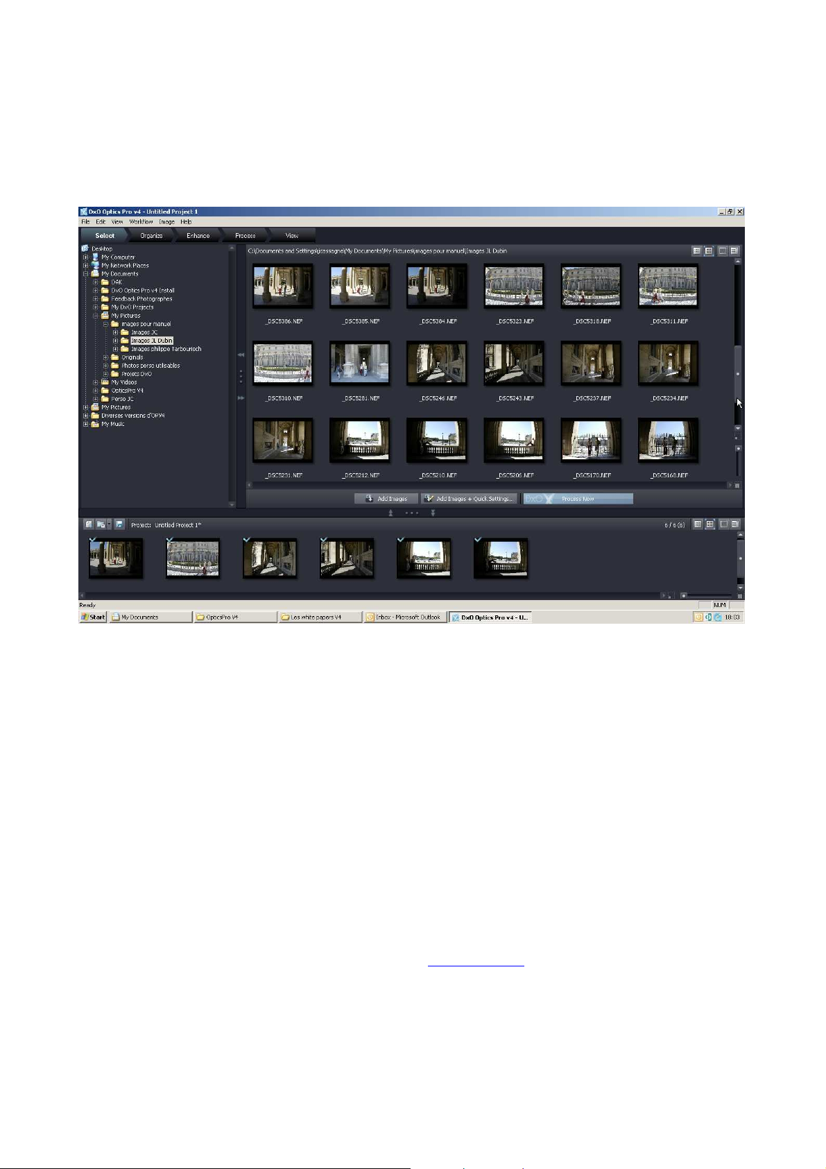
When you first launch the application, the ‘Select’ tab is the only one that is active (highlighted), and your workspace displays a familiar Windows Explorerstyle browser where the top two panes (resizable) allow you to navigate around the files on your disk or accessible externally. As usual, in the righthand file pane you can click on a column header to organize files according to that criterion, and the top bar of the active column header has an

 or  arrow

to select ascending or descending sort order.

Adding images

This initial ‘Select’ stage involves adding the photos you want to process to the project pane, which will remain in the lower part of the window throughout all five stages (from Select to View). As you add images, they are displayed as thumbnails in the bottom pane, which you can resize if necessary to fit in a useful number. Besides using the mouse to drag the dividers to resize these panes, they each have rather discreet  and buttons, to fully open or close a pane, and a  button to regain mouse control.

Page 10

DxO Optics Pro V4.2 Reference Manual

The header strip for the project pane at the bottom of the screen has four buttons at the far right. The first two let you change between viewing as thumbnails or as a classic ‘details’ file list; the last two select respectively

filters you can use to organize your thumbnail display, and which parameters

are displayed in ‘list’ mode. The same buttons appear at the top left of the right-hand ‘files’ pane, where they perform the same functions.

Star-ranking

Also on the project pane, tucked away discreetly at the bottom right, is a small slider, with a button at each end; dragging this to the right, or clicking the right-hand end button, increases the thumbnail size displayed, while dragging it to the left or clicking the left-hand button reduces the size back down to the default. You can choose to ‘

rank’ your images, in order to set their priority for

processing, and also, to save clutter, you can create a ‘stack’ of perhaps related images, or images to which you want to apply the same set of corrections. Both these commands are accessed under the ‘Image’ drop-down menu. In addition, to rank your images for processing priority, you can simply click on the appropriate number of stars displayed above each thumbnail (this works in any of the workspaces, except of course ‘View’).

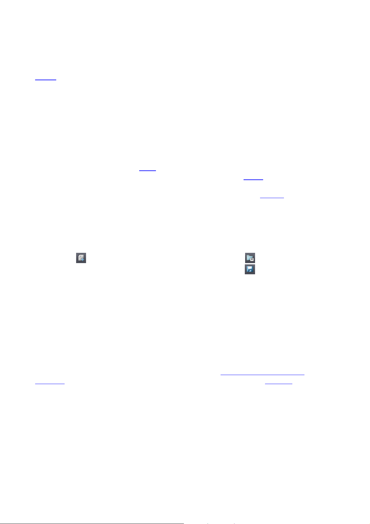
On the left of the project pane header bar are three more buttons, for managing your project; your project name is displayed just to the right of

them. The button lets you create a new project, the one lets you open

an existing project (provided any exist, of course), and lets you save and/or rename a project.

At the bottom of the right-hand ‘files’ pane are three important buttons — ‘Add images’, ‘Add images and Quick settings’, and ‘Process now’. Note that these buttons will be grayed-out and inactive until you have at least one image selected (in the case of the first two), or at least one image in your project (for the last one).

‘Add images’ will add one or more images selected in the file pane — the usual selection shortcuts apply: Shift + click to select a whole range and Ctrl + click to make multiple selections — into your project. ‘

Add images and Quick settings’ does the same, except that it allows you to choose ‘presets’ to be

associated with particular images.

The simplest way of adding images is just to drag them down from the file pane into the Project pane. This , of course, does not work if you want to associate a preset with the image.

Page 11

DxO Optics Pro V4.2 Reference Manual

The thumbnails and their buttons

To remove one or more images from your project, you simply click on the

orange icon displayed in the centre below each thumbnail; if multiple images are selected, clicking the on any one of them will delete the entire

selection in one go. You can select a group of adjacent images by dragging a ‘rubber-band’ box around them with the mouse, or by holding down the Shift key as you click on the first and last images in a series. Multiple non-adjacent images can be selected by holding down the Ctrl key while you click on them.

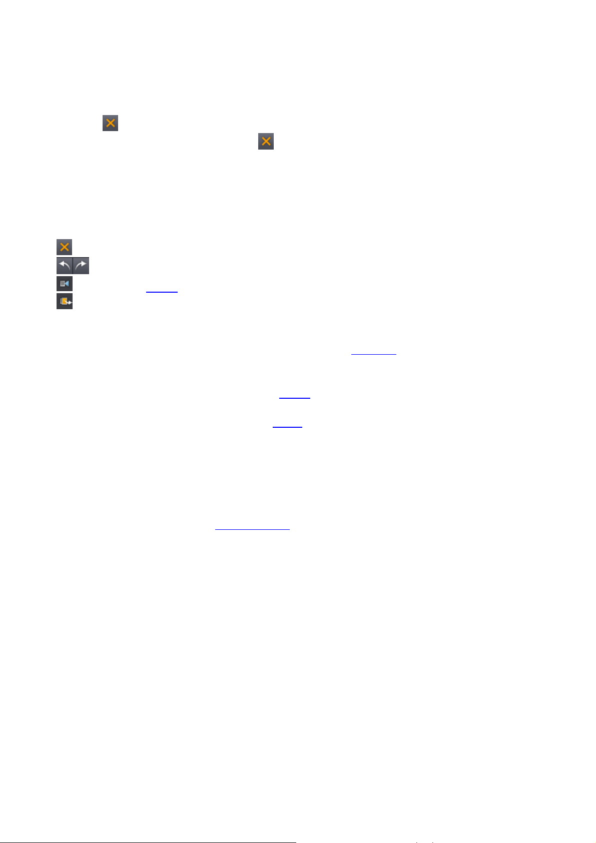
The buttons associated with each thumbnail offer the following functions:

to remove the image from the current project

to rotate the image for correct viewing orientation

to create a stack (active on the last-selected image of a multiple selection)

unstacks a stack of images (active when a stack is selected)

Above each image, only visible on mouse-over, are a line of stars  (grayed out at start-up) to indicate the selected ranking of this image for processing — you can click these stars on or off at any time.

In addition to these buttons, certain icons may appear above each thumbnail — follow the link to discover the meanings of these, as they give important information about each image. The color of the frame surrounding the thumbnail also has a significance.

Fully automatic operation

Once you’ve selected and added to your project all the images you want to process, if you have no need to make any manual adjustments to your images, you can simply press the ‘

Process now’ button, and processing will take place

automatically. You will only be asked to intervene manually to input particular data in the event of certain corrections where DxO does not have enough information to process correctly.

Page 12

DxO Optics Pro V4.2 Reference Manual

Chapter 3— Organize your images on an electronic

light-table

Once you have established a Project (either by re-opening an existing one, or by creating a new one), you can use the ‘Organize’ workspace to organize your images and their subsequent processing. If you only have a few images to process, you may be able to skip this stage completely, but it is extremely helpful where your workflow involves much larger numbers of images!

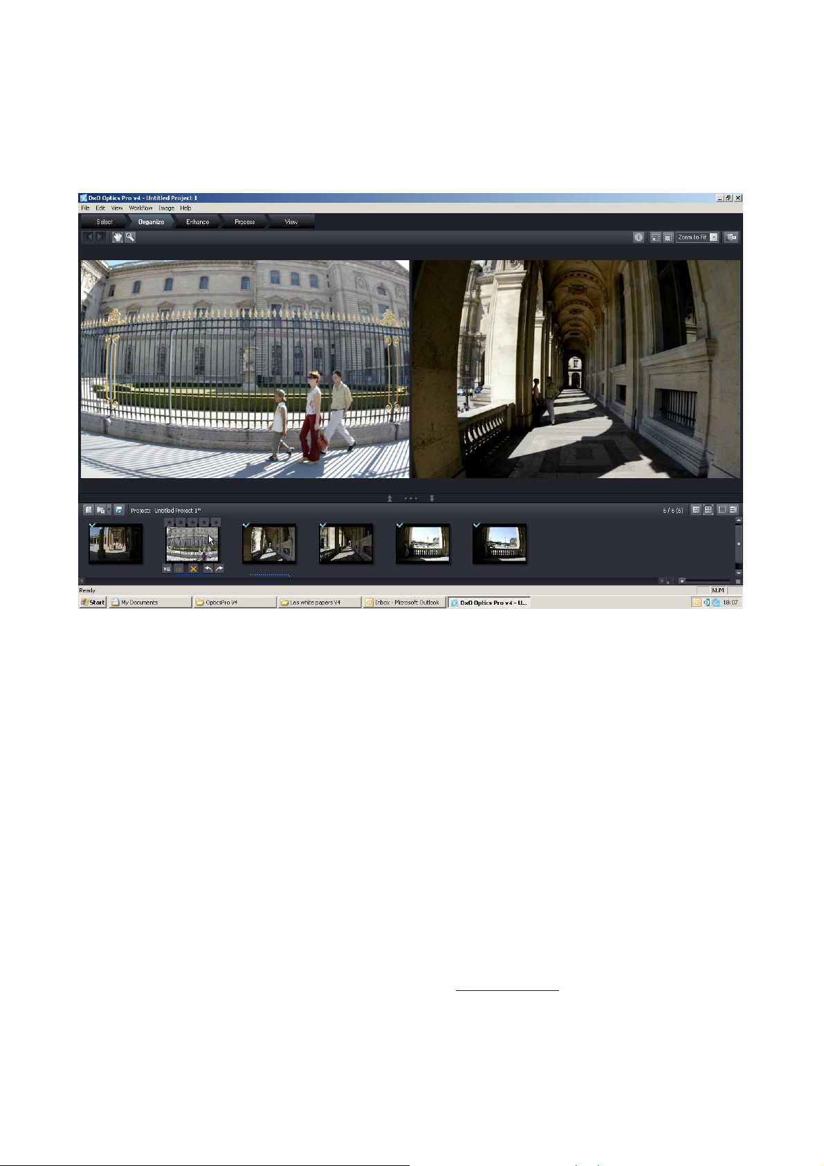
In the ‘Organize’ workspace, the top half of the screen (as always, resizable) is available as a sort of ‘light table’ to display one or more images selected for preview. You can transfer any image to the preview window simply by leftclicking once on the relevant thumbnail. You can select multiple images to preview at the same time, and if for any reason you want to empty the preview screen, you just have to click on a blank area of the thumbnail pane.

The big picture

As soon as there is an image in preview, the with its thumbnail appear at the bottom right of the workspace, along with the current filename on the left. At the left-hand end is a ‘thumbtack’ button that will ‘stick down’ the preview image; this means you can move around between

icon buttons originally associated

Page 13

DxO Optics Pro V4.2 Reference Manual

the thumbnail images in your project pane, without the preview pane continually refreshing.

At the top of the workspace is a header bar. On the left-hand end of it are two buttons: a ‘hand’ tool that lets you grab and drag a zoomed-in preview image so as to be able to examine any part of it; has no effect in ‘Zoom-to-fit’ mode.

Next to it is a magnifying glass tool that lets you to zoom in to any part of the image by successively clicking on it; holding down Shift as you click turns it into a zoom out tool. In all cases, the minimum zoom size is ‘Zoom to fit’ (i.e. determined by the size you have set your preview pane to), and the maximum is 200%.

Alternatively, over on the right-hand side, a drop-down list lets you choose the zoom ratio of the preview image — ‘zoom to fit’ will show you the whole image, resized according to the format of the image and the screen space available, while the various other ratios allow you to examine part of the image in greater detail; as an alternative to selecting from the drop-down menu, you can use the ‘zoom in’ and ‘zoom out’ buttons.

There is also an  button that toggles on/off the display of image EXIF data on the left-hand side of the preview screen.

Adapt your workspace

Also on the right is a little icon you can click to activate a ‘

background brightness’ slider, allowing you to set the background visible around the image

anywhere you like between black and white (at start-up, the default is around 18% gray). This is helpful as a neutral reference when assessing or adjusting the color balance of your images.

If you have a large number of images to process, you will find the ‘Organize’ workspace very useful in allowing you to examine and organize your images in this way, and from the ones you have loaded, make a second, finer selection using the larger ‘light table’; you may well want to reject certain images and discard them from your project,

stack them, and/or assign a processing

priority by ranking your images — later, at the processing stage, you will be able to choose which ranks to process, or not. Both these commands are accessed under the ‘Image’ drop-down menu, or via the thumbnails themselves.

Once you have had this chance to compare and organize your images, you can of course start automatic processing right away (‘Start Processing’ command from ‘Workflow’ menu, or keyboard shortcut Ctrl + R) — but it’s more than likely that you’ll want to move onto the next step, which is to make manual adjustments to some of the correction parameters, or apply some preset corrections to your images.

Page 14

DxO Optics Pro V4.2 Reference Manual

palette

Chapter 4 — Enhance your images using

DxO Optics Pro tools

Tools

Corrections

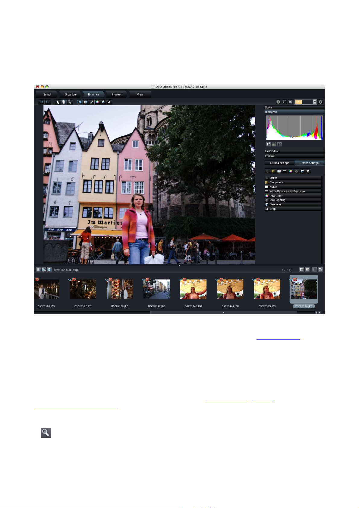
In the ‘Enhance’ workspace, you will immediately notice that some things have changed. For a start, on the right-hand side of the screen, a palette area appears, which is where you will find all the correction and adjustment tools. We’ll come back to look more closely at that in just a moment, but for the time being, let’s just make a quick tour of the other new items in this workspace.

As always, the familiar project pane occupies the lower part of the window.

The header bar, on the right, carries the same information, zoom, and

background brightness buttons as for the Organize workspace. On the left, the

‘hand’ tool that (lets you grab and drag a zoomed-in preview image so as to be able to examine any part of it) has no effect in ‘Zoom-to-fit’ mode. Next to it is

tool that lets you to zoom in to any part of the image by clicking on it;

a holding down Shift as you click turns it into a zoom out tool. In all cases, the minimum zoom size is ‘Zoom to fit’ (i.e. determined by the size you have set

Page 15

DxO Optics Pro V4.2 Reference Manual

your preview pane to), and the maximum is 200%. Note that some corrections cannot be previsualized with zoom factors below 75% (this is the case for the Chromatic Aberration, DxO Lens softness, DxO Noise and Unsharp Mask corrections). You’ll find two buttons that specify the way your preview image is displayed:

display both ‘before’ and ‘after’ images in preview window

display ‘after’ image in preview window; the “before” image will

replace it while you maintain the left mouse button pressed on it. But there’s also a whole new group of four buttons, whose functions will be described later as we go through the tools palette.

Corrections Palette

Now let’s go and take a closer look at the corrections and adjustments that are accessible via the palette on the right-hand side. Don’t forget, in the description that follows, just like everywhere else in this Guide, you can click on the links indicated to obtain further details about a particular topic. Throughout the tools palette, you can click on the title bar to expand or shrink each tab at will; the title of opened tabs is shown in bold, to help you find your way around more easily. 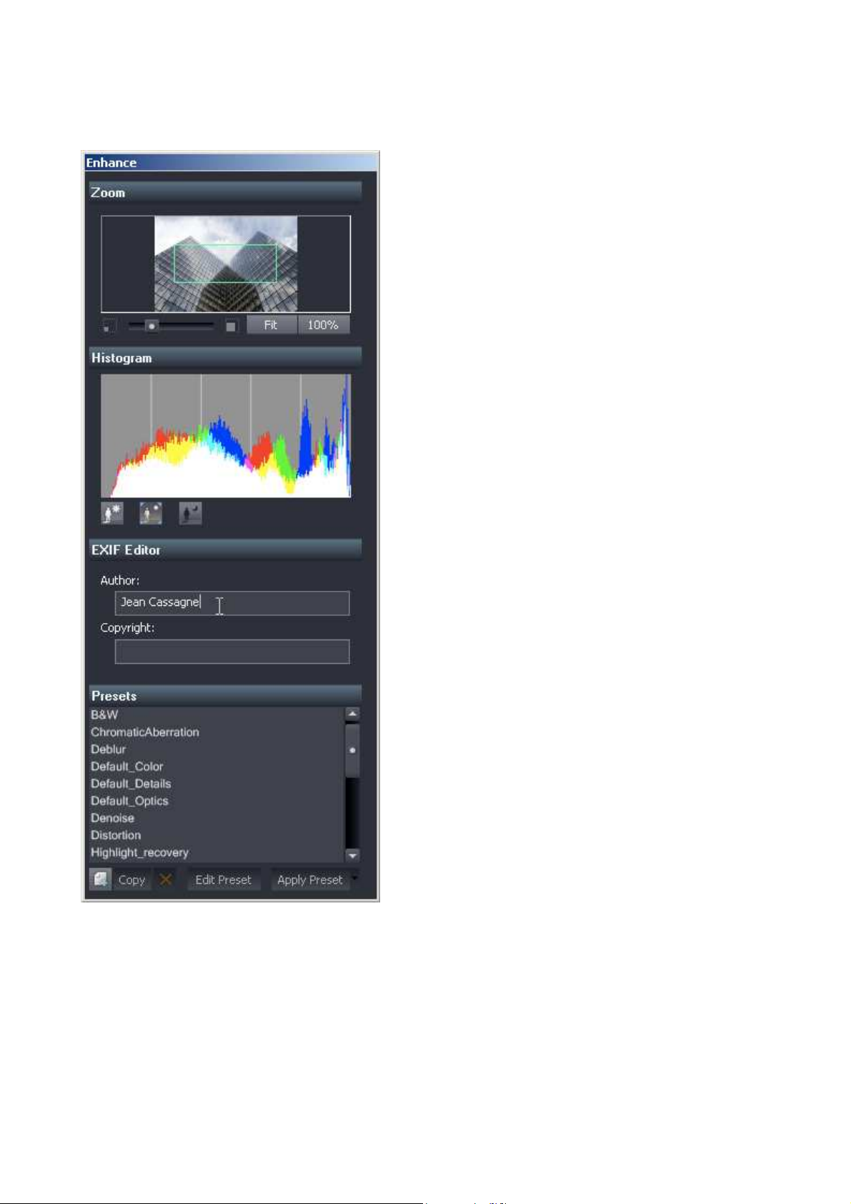At the top comes the tools palette with four basic tabs:

Zoom has a small window that indicates the visible part of the image with a

green box that represents the assigned size of the preview area. As you would expect, the more you ‘zoom in’, the smaller the green box appears (you are looking more closely at a smaller part of the image). You can grab the box with the mouse to drag it around the screen in order to examine specific parts of an

image. The

button on the left hand end of the header bar lets you grab the main preview image to move it around when zoomed in. There is the same zoom slider as before, together with small zoom in/out buttons at either end. Maximum zoom in all cases is 200%, while the minimum zoom size depends

on the size you have set the preview pane to. The button in the header bar is another way of zooming in and out.

Histogram gives a graphical representation of the distribution of the relative

brightness levels in the image, across the red, green, and blue color channels. A very useful tool, you will probably find yourself leaving this open a lot of the time while you are adjusting color and exposure!

EXIF Editor brings up a tab with two text fields, where you can enter specific

information that will be added to the EXIF header. They concern the author and the copyright information of the picture.

Presets opens a small window with a list of available presets you can apply to

your image — you can apply all of the settings from a selected preset, or select

Page 16

DxO Optics Pro V4.2 Reference Manual

which particular corrections you wish to use. Of course, there is nothing to stop you from adjusting these same parameters manually later, in which case the preset values will be over-ridden for this particular image. Here, you can also perform elementary preset management operations.

Guided or Expert?

Immediately below these four tool tabs, there are two large buttons for ‘Guided settings’ and ‘Expert settings’.

‘Guided settings’ replaces the full corrections palette with a list of the four main correction groups: Optics, Sharpness, Color and Lighting. Alongside each of these is a drop-down menu where, in addition to the default ‘As shot’ (effectively, ‘automatic’), you can select from a list of any

custom presets you

may have saved. In this way, you might choose, for example, to apply the Lighting corrections stored in one preset, and the Color corrections stored in a different one. ‘Expert settings’ opens a ‘palette’ with access to the full range of corrections and adjustments, as detailed below. First there is a strip with eight buttons that open the eight corrections panels below. If the tab you want to open is hidden off screen because of other open tabs, these buttons are useful in letting you go straight to the panel you want, closing any others that are open. You can also open and close any panel just by clicking on its title bar tab.

Eight Correction palettes

Then, there are the eight principal tabs for the main groups of corrections. Note that under each tab certain corrections may not be available, depending on the images and correction modules you have loaded — the title of available corrections is shown in bold white text, whereas de-activated corrections are grayed out and not bold.

DxO Optics — the corrections for geometric distortion, chromatic aberration, purple fringing, and vignetting

Sharpen — DxO lens softness correction to correct for measured lens

characteristics and unsharp mask, to provide intelligent overall sharpening for images where no lens-specific module is available.

DxO Noise — noise reduction, minimizing both general and impulse noise

White balance and Exposure — white balance lets you adjust the overall color

balance of your images, either to correct for lighting color balance, or perhaps to create a specific effect. Exposure control with highlight recovery allows postshooting exposure adjustment, as well as offering the possibility of recovering apparently ‘lost’ highlight detail (with Raw format images only). You will use

here the White Balance Tool

located on top of the window.

Page 17

DxO Optics Pro V4.2 Reference Manual

DxO Color — enables you to adjust your colors in the Hue / Saturation / Lightness domain, which although not always the easiest or most intuitive to

use, has the advantage of allowing you to enter numeric (and hence repeatable) values very easily. Here you also have access to a powerful tone-

curve manipulation function that lets you adjust both the overall master tone

curve and the individual color channel curves, for absolute maximum flexibility. Two brand new features here are Color rendering and Color matching. The former lets you apply a specific ‘look’ to your images, starting right from the very ‘look’ of specific camera bodies, along with preset contrast and color saturation options, and some special presets: portrait and landscape, together with black & white and sepia effects. Color matching is a sophisticated way of achieving exact color matching between shots, even where a neutral color reference is missing. The system allows you to pick up to four colors and set the color they are each meant to reproduce as, and then DxO Optics Pro will make a best-compromise calculation to adjust the color balance of the entire image — what’s more, it can do this across a whole string of images, making it is easier than ever before to match critical colors between different shots. The Multi-Point Color

Balance tool

is located on the top left of the window.

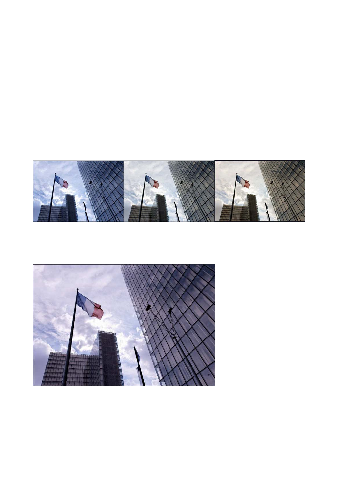
DxO Lighting — corrects image contrast in an intelligent, adaptive way, using

global and local contrast adjustment to bring out shadow, mid-tone or highlight detail that might otherwise be lost. A ‘Fine settings’ button within this panel accesses additional controls for even more precise adjustment.

Geometry — corrections for Volume Anamorphosis Correction and Keystoning / Horizon. The former is a lens-dependent correction that is related to geometric

distortion. Being subject-matter dependent, this adjustment requires manual setting of the type and amount of correction. The remaining corrections provide adjustments to compensate for

keystoning

in both vertical and horizontal planes, image rotation (horizon correction),

scaling (image sizing) and H/V ratio (stretching / squeezing of

horizontal / vertical proportions). Clearly, these are entirely image-dependent and so do need to be set manually, with the help of the Keystoning – Horizon

tool located on top of the window.

Crop — last, but not least, here you can edit the composition of your image,

with the option to constrain the proportions to those of the original shot or certain preset formats, or to allow unrestricted cropping to custom formats. Click on the Crop Tool (top of the main window) to access this function.

When you have finished making any manual adjustments and/or applying any presets, the next logical step will be to start processing your images. You can click on Ctrl + R at any time, or select the Start Processing command from the Workflow menu, but, more than likely, you’ll want to move onto the next step by clicking on the ‘Process’ tab to select the appropriate workspace.

Page 18

DxO Optics Pro V4.2 Reference Manual

Chapter 5 — Process as many images as you want

with just one click

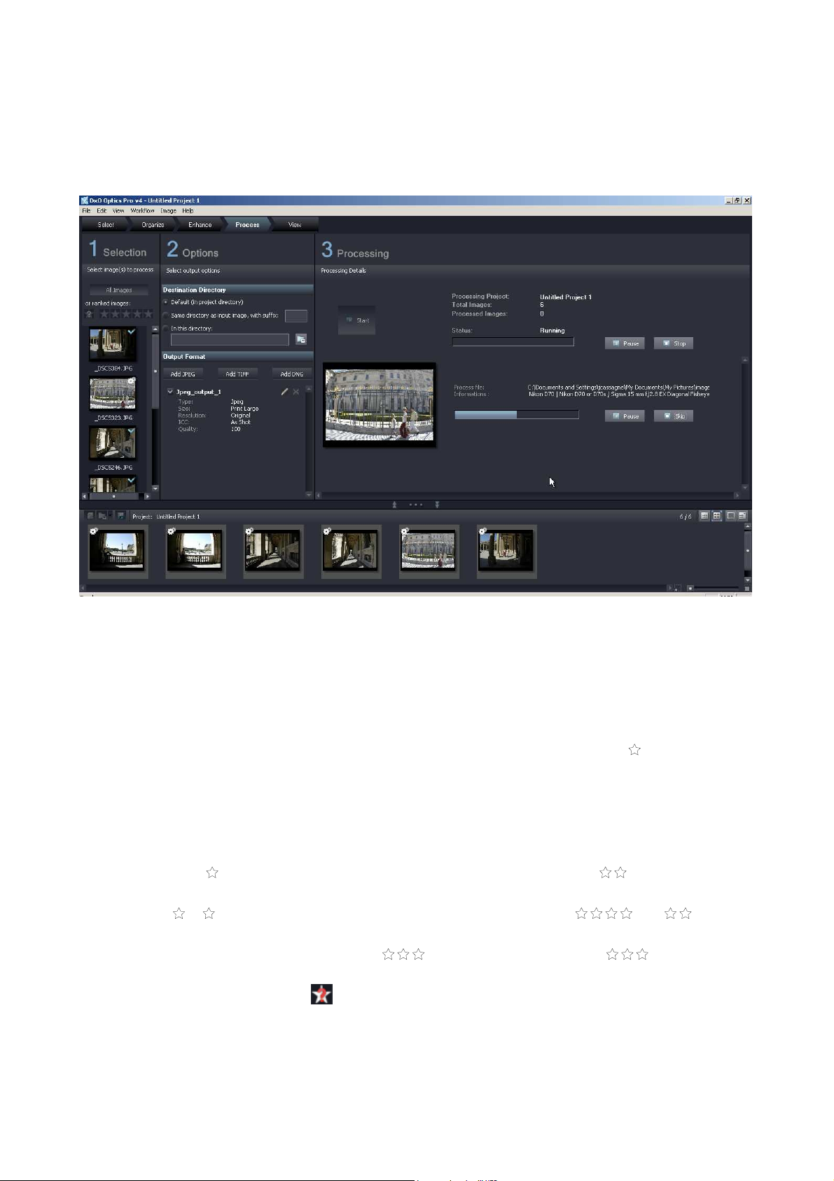
The top part of the ‘Process’ workspace is divided into three areas, plus the familiar Project pane at the bottom.

In the left-hand area ‘1-SELECTION’, you can implement the ‘star ranking’ you set earlier (and can still do in this workspace, since the thumbnails are still available); this is where you select which rank of images to process. There is a button for ‘All’, or you can again click to activate 1, 2, 3, 4, or 5 (individually, or in combination).

Process the stars

You can select a higher-ranking star alone to specifically exclude lower rankings; so   will process only those images ranked . You can also make multiple selections, just by clicking on the corresponding stars; so for example   , will process only images ranked either or .

To process all images ranked up to , you need to select . Minithumbnails of the selected images will appear in the column below. Alongside

the star buttons is another button, which allows you to select only unranked images for processing.

Page 19

DxO Optics Pro V4.2 Reference Manual

The centre area ‘2-OPTIONS’, under ‘Destination directory’, has radio buttons for using either the default project directory or a specific directory — the browse button to the right opens a browser window where you can select an existing directory or create a new one.

Define output formats

Below this are three buttons for adding and/or selecting one or more output image formats. Each button (JPEG, TIFF, DNG) opens a dialog box with settings appropriate to that format. A summary of all available formats is shown, and you can click on

or  to enable or disable them for this batch.

You must have at least one output format active for processing to commence, otherwise you will see an error message when you press ‘Start’.

The right-hand area ‘3-PROCESSING’ has a big Start button, and gives status information about the progress of your project, along with controls to either ‘pause’ or ‘stop’ (i.e. abort) processing.

As soon as you click on ‘Start’, if you have not already saved your project since the last changes were made, you will be prompted to save it before proceeding.

You are kept informed of progress in processing your project by means of two progress bars, the top one showing the overall progress of the project as a whole, and the lower one indicating progress on the current image. During processing, upper ‘Pause’ and ‘Stop’ buttons allow you to halt processing temporarily or abort it altogether. Lower buttons similarly allow you to ‘Pause’ processing of the current image, or ‘Skip’ it altogether.

While processing is under way, the thumbnails of all images included for processing carry a [two cogs] icon. Once processing is completed, these change to a

 indicating that processing has been successful.

Page 20

DxO Optics Pro V4.2 Reference Manual

Chapter 6 — View the results of your work

(with a little help from DxO)

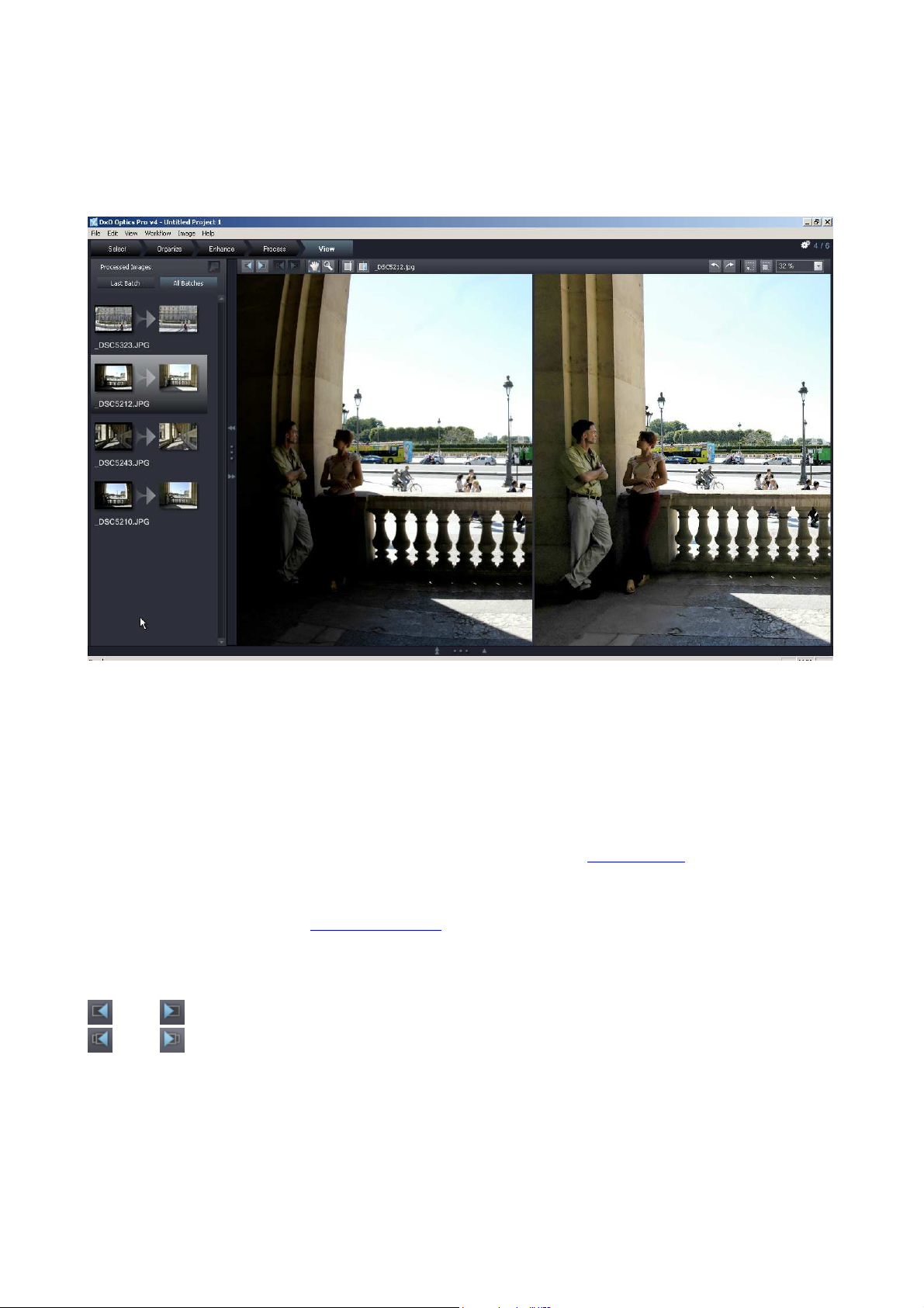
The ‘View’ workspace has the now-familiar three resizable panes; the top lefthand pane shows before/after pair thumbnails of all your processed images, with buttons to skip to ‘Last batch’ and ‘All batches’. The image pair being viewed has a highlighted background.

The header bar in this workspace has, on the left-hand side, a [projector] button that gives access to the options for running a processed images. To the right of this is shown the (original) filename of the image displayed. To the right-hand end of the header bar are nine buttons, plus the usual group of zoom controls.

Here’s what they do:

and display previous / next image

and display next / previous output image — if you have selected more than one output format for a given image, lets you view the JPEG / TIFF / DNG images in turn. When you have reached one end or the other of the image series, the relevant button will be grayed out.

slide show of the

Page 21

DxO Optics Pro V4.2 Reference Manual

Chapter 7— How to go further

After going through a full typical session, you may want to explore more options. The powerful new DxO tools bring you many functions that you can fine tune in your own way. In the following chapters (that you’ll find only in the electronic version of this user guide), you can discover the various settings that can be applied to your photos and how you manipulate the corresponding palettes. Remember that your original picture is never modified: you can always create a new project, along with different settings applied to the same image or group of images.

Your workflow

Another point of interest concerns the way you integrate DxO Optics Pro to your personal workflow. You may use an image management software to download, index and preview your photographs. You may also invest in some heavyweight treatment and correction software, (whose name begins for instance with photo and finishes by shop). DxO Optics Pro must be used ahead of the latter, whose importance will be greatly reduced and, concerning the database software, you should make sure that the EXIF information stored in the image file has remained untouched. If not, you’ll prefer running your pictures through DOP before managing them with another package.

Thank you for using DxO Optics Pro V4! You will find more information on the pdf version of this user guide, and in the Frequently Asked Questions available on DxO’s website:

http://www.dxo.com/en/photo/support

Page 22

DxO Optics Pro V4.2 Reference Manual

Chapter 8 Menus

File / Edit / View / Workflow Image Menus

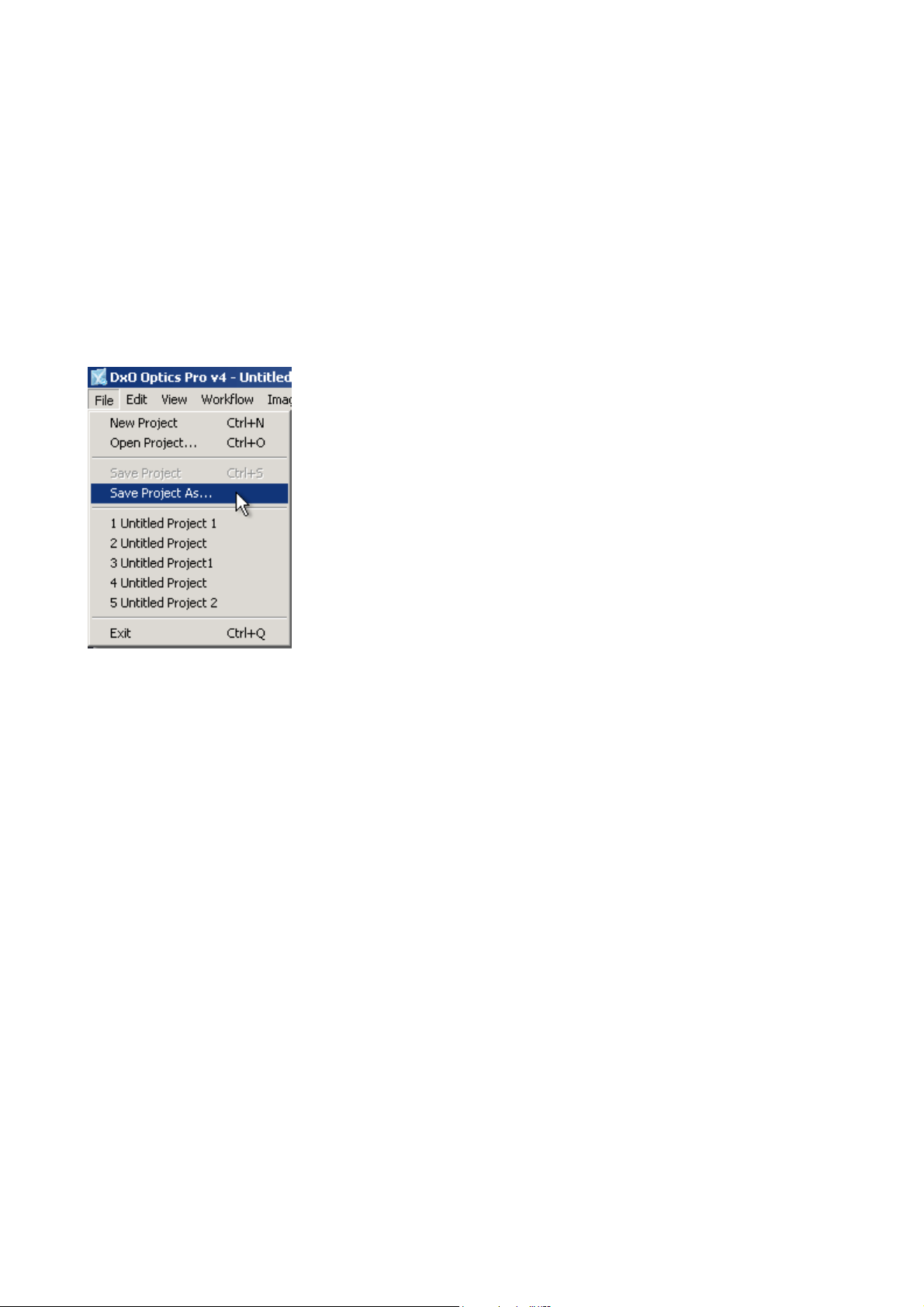
The File menu includes commands to :

Create a new project [Ctrl + N] Open an existing saved project [Ctrl + O] Save the current project [Ctrl + S] Save the current project under another filename

Along with a list of the most recently used projects

Exit is also available from this menu [Alt + F4]

It’s important to note that a ‘project’ saves all the current settings of your user interface, along with the list of images selected and the Output formats settings, but does not save duplicate copies of these images. So saving a project is fast, and does not use up a significant amount of disk space. It is very handy to be able to keep all your settings and come back to them later.

The command, « Export image for ICC profile » permits you to create a version of the image selected, adapted to the creation of an ICC color profile from third-party software. Two options are possible: “Export in linear RAW” respects the information received by the captor, without interpreting the colors other than for the White Balance adjustments, in order to create a specific profile for

Page 23

DxO Optics Pro V4.2 Reference Manual

the camera body used for this image. “Export in DxO Natural”: converts, on the other hand, the colors abstracting from the camera’s rendering: the profile can be applied to an image no matter what camera body was used to create it. In order to call up such profiles, you only need to import them under the tab “DxO Color” of the step “Adjust”.

The Edit menu

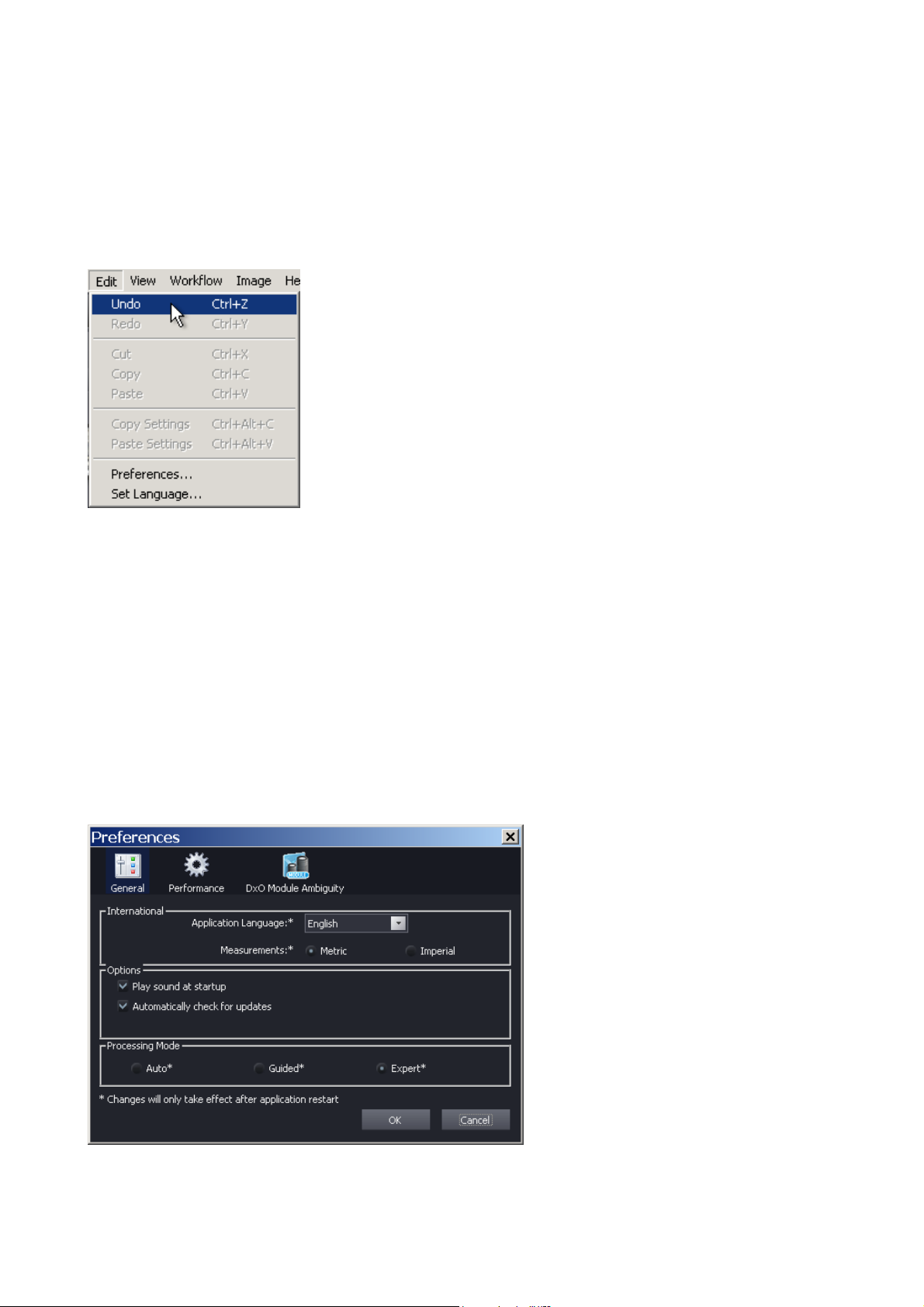
A very useful pair of commands, Undo [Ctrl + Z] and Redo [Ctrl + Y] apply to the last action you’ve performed.

The classic Cut [Ctrl + X], Copy [Ctrl + C], and Paste [Ctrl + V] commands allow you to edit certain items like numerical values, names etc.

The Copy settings [Ctrl + Alt + C] and Paste settings [Ctrl + Alt + V] commands allow you to copy all the correction settings from a given image onto another image or group of images.

The ‘Preferences’ command accesses adjustments to certain overall working parameters, via three tabs:

General tab

Page 24

DxO Optics Pro V4.2 Reference Manual

Here you can select the working language, choose whether you prefer to use metric or imperial units for measurements, and select if you want the camera shutter sound to play at start-up. You can also select / deselect automatic checks for software updates.

Processing Mode

Radio buttons here allow you to choose which mode of processing best suits your way of working, if necessary changing the choice you may have made at the time of installation. Please refer to the description of these three modes given earlier.

Changes made here only come into effect the next time you start the program, so if you want them to take effect immediately, you will need to exit and restart the program.

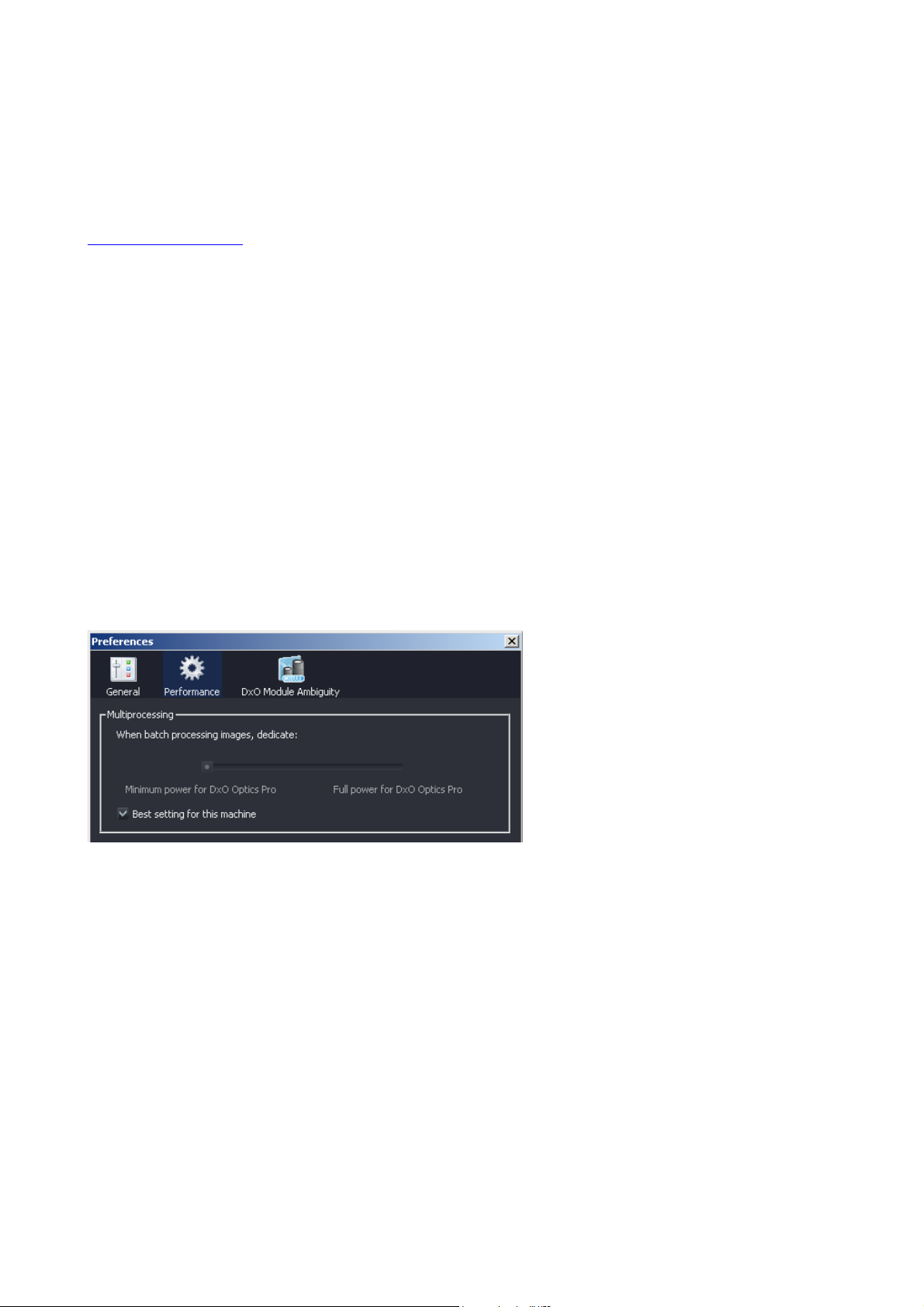
Performance tab

Settings for optimizing performance during batch processing. A slider lets you choose between maximum reactivity or fastest processing speed, with a checkbox to allow the setting to be determined automatically for your particular machine.

Module ambiguities tab

Under certain circumstances, it may happen that an image’s EXIF data doesn’t contain enough lens information for DxO Optics Pro to determine the right Correction Module to use for this image. This will normally be flagged at the time of adding images to your project, and you will be asked to tell DxO Optics Pro exactly which lens was used for a particular shot, so as to pick the correct module.

Page 25

DxO Optics Pro V4.2 Reference Manual

You can also resolve such ambiguities via this tab under Preferences. Where ambiguities exist, the offending modules will be listed, and you can choose the one you’re actually using. You are given the option of choosing based on one particular image, or on one particular processing batch, or it may be that you will want to always assign this particular module in this way—depending of course on the specific combinations of bodies and lenses that you habitually use.

View

The View menu offers the option of switching between displaying thumbnails [Ctrl + Shift + I] or a list of file details [Ctrl + Shift + R] — in the ‘Select’ workspace, this applies to either the right-hand ‘file’ pane or the bottom ‘project’ pane, depending on which one you click before using the command. In the other workspaces, it will of course only affect the display in the bottom ‘project’ pane.

You can also check the options to display Raw files, RGB files, or corrected files; unchecking an option means that files of this type will not be displayed; do note that it is not possible to uncheck all three file types at once, and the system will not allow you to select a single file type alone if there are no files of this type in your current project.

Status bar toggles on and off the status bar at the bottom of the screen.

Split gives direct mouse control of the project pane divider — this is very useful for bringing it back on screen quickly if you have minimized the project pane to enlarge the preview pane, for example.

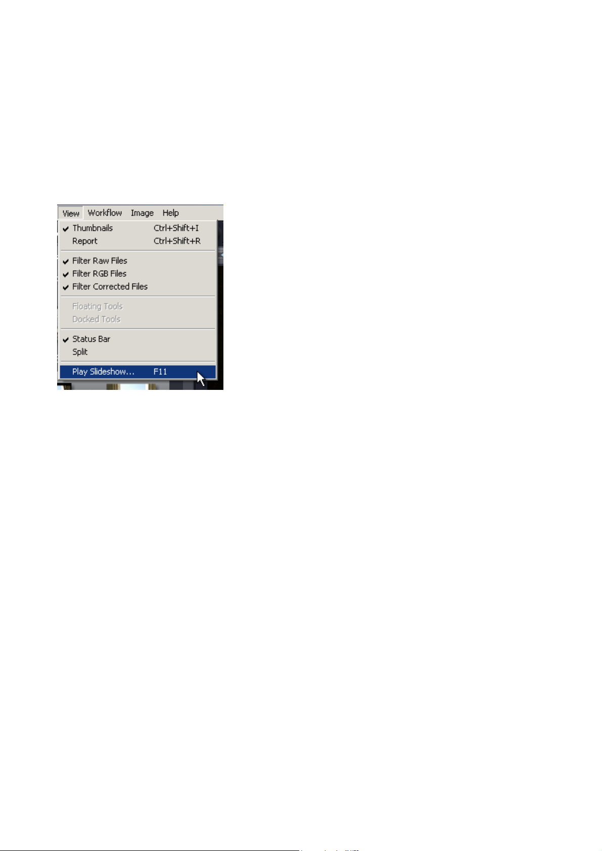
Play slide show [F11] brings up a little control panel so that you can display an automatic, full-screen preview sequence of all the images in your current project.

Page 26

DxO Optics Pro V4.2 Reference Manual

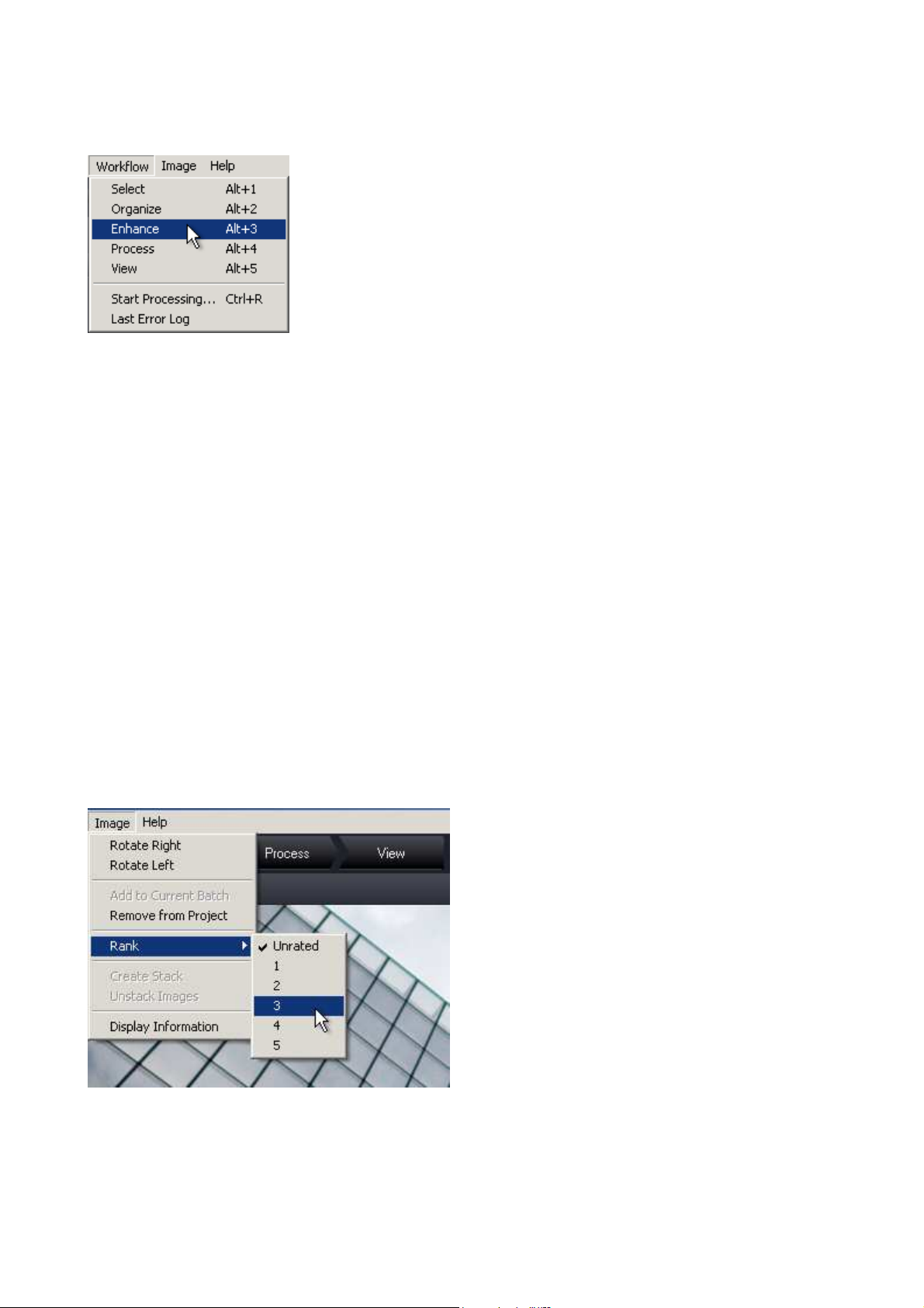
The Workflow menu includes commands for switching directly between the five workspaces (exactly the same effect as the tabs):

Select [Alt + 1] Organize [Alt + 2] Enhance [Alt + 3] Process [Alt + 4] View [Alt + 5]

You can select these at any time, and your workspace layout changes to suit. If you have already selected ‘Auto’ mode (Edit > Preferences), you cannot access the Enhance tab, which will disappear, and the Enhance command here will be grayed out. This setting can be changed in Preferences, under the Edit menu.

In addition, there is Start processing [Ctrl + R], which you can use in the event of fully automatic processing of a particular batch of images.

Image Menu

The Image menu offers the possibility of rotating your image left (counterclockwise) or right (clockwise) in order to be able to view portrait images with the correct orientation.

Page 27

DxO Optics Pro V4.2 Reference Manual

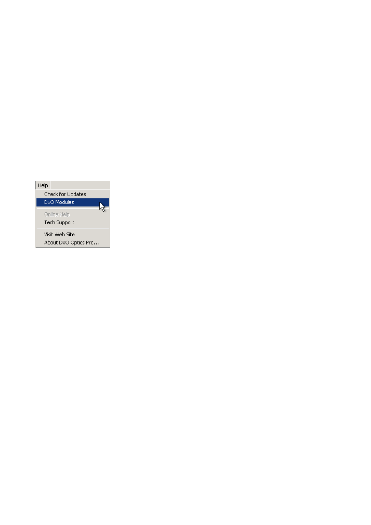
Likewise, you can use the commands here to ‘rank’ a selected image or group of images according to a rating of one to five ‘stars’; when you get to the processing stage, you can select which images you wish to process in a given

batch according to your defined star ratings.

If you have at least two images selected, the Create stack command becomes available, and will make a stack of the selected images; likewise, if you select an existing stack, you can use the reverse command, Unstack images, to open out the stack again into its individual images.

The ‘Display information’ command has the same effect as the  button on the toolbar, toggling on/off the display of the EXIF and thumbnail information in the preview window — this command is only applicable in the ‘Organize’ and ‘Enhance’ workspaces, and so is disabled in the other three.

The Help menu offers access to an ‘About DxO Optics Pro’ information screen containing information about the exact software version, important if you need to contact DxO Technical Support.

There are also direct links to the general DxO website, and the software update and technical support pages.

Page 28

DxO Optics Pro V4.2 Reference Manual

Chapter 9 Using Auto, Guided and Expert modes

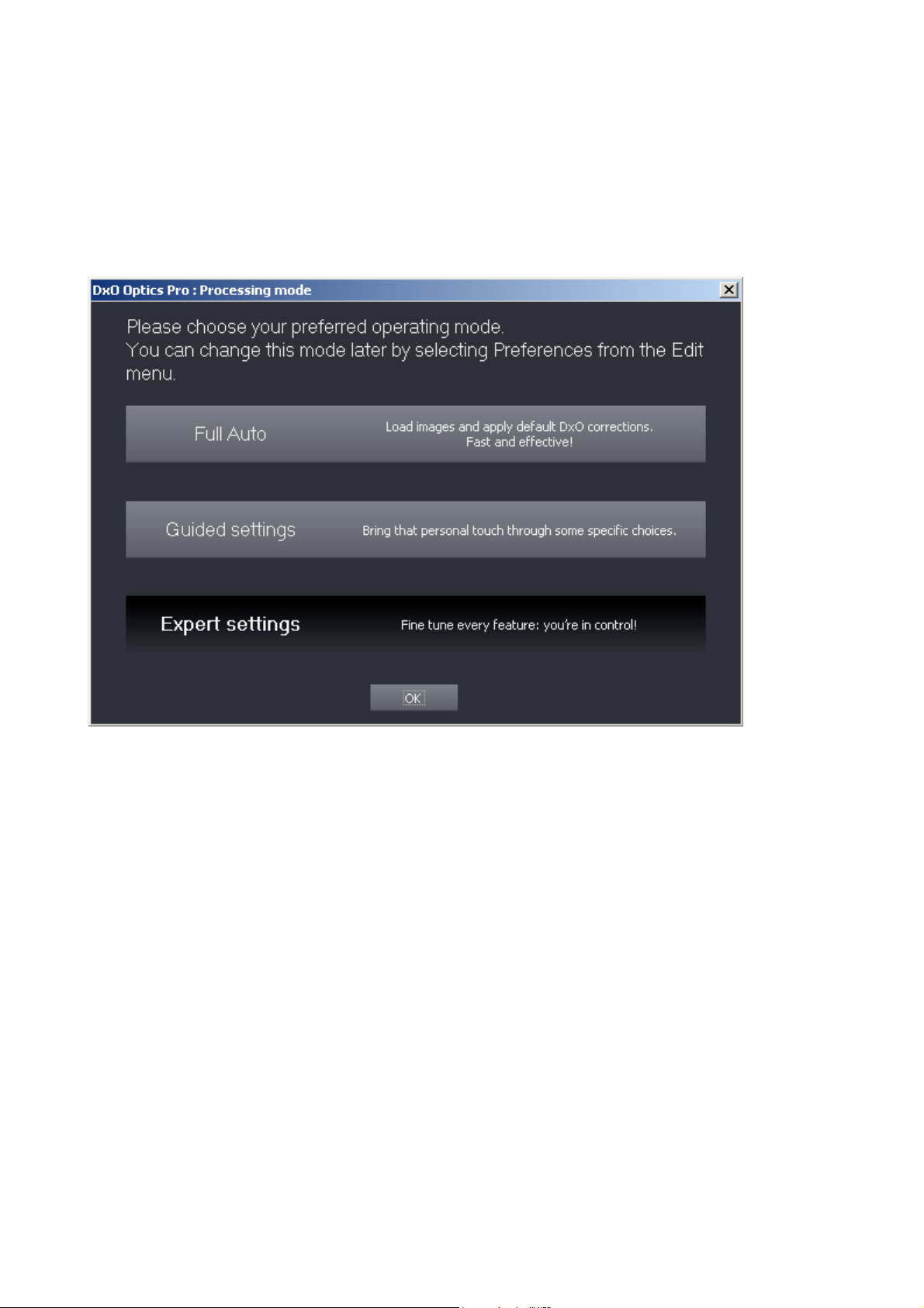
Processing mode

The first time you run the program after installation, you will see this screen:

Here you are prompted to choose the processing mode that is most suited to your preferred way of working:

Auto mode

DxO Optics Pro will determine automatically the optimum correction settings for your images, and the only input required from you will be to fill in certain information where EXIF data is missing or insufficient. In this mode, the 'Enhance' step is disabled (its tab will be grayed out), and after selecting and organizing your images, you will move straight on to process them automatically.

Guided mode

In this mode, the ‘Enhance’ step will be available, but instead of having access to the full set of manual correction adjustments, you will be offered the choice of applying the four main groups of corrections according to drop-down lists of preset choices, including of course access to your own saved presets. You will be able to switch over to ‘Expert Settings’ mode at any time via the

Page 29

DxO Optics Pro V4.2 Reference Manual

button available under the ‘Enhance’ tab.

Expert mode

As you might expect, this mode gives you access to all the manual and automatic correction settings. The ‘Enhance’ tab will be enabled, and the full range of correction tabs will be accessible. You will be able to switch over to ‘Guided Settings’ mode at any time via the button available under the ‘Enhance’ tab.

By default, the ‘Expert’ mode is selected, and once the application has been run for the first time, you can always change the settings again in the future under Edit > Preferences > General.

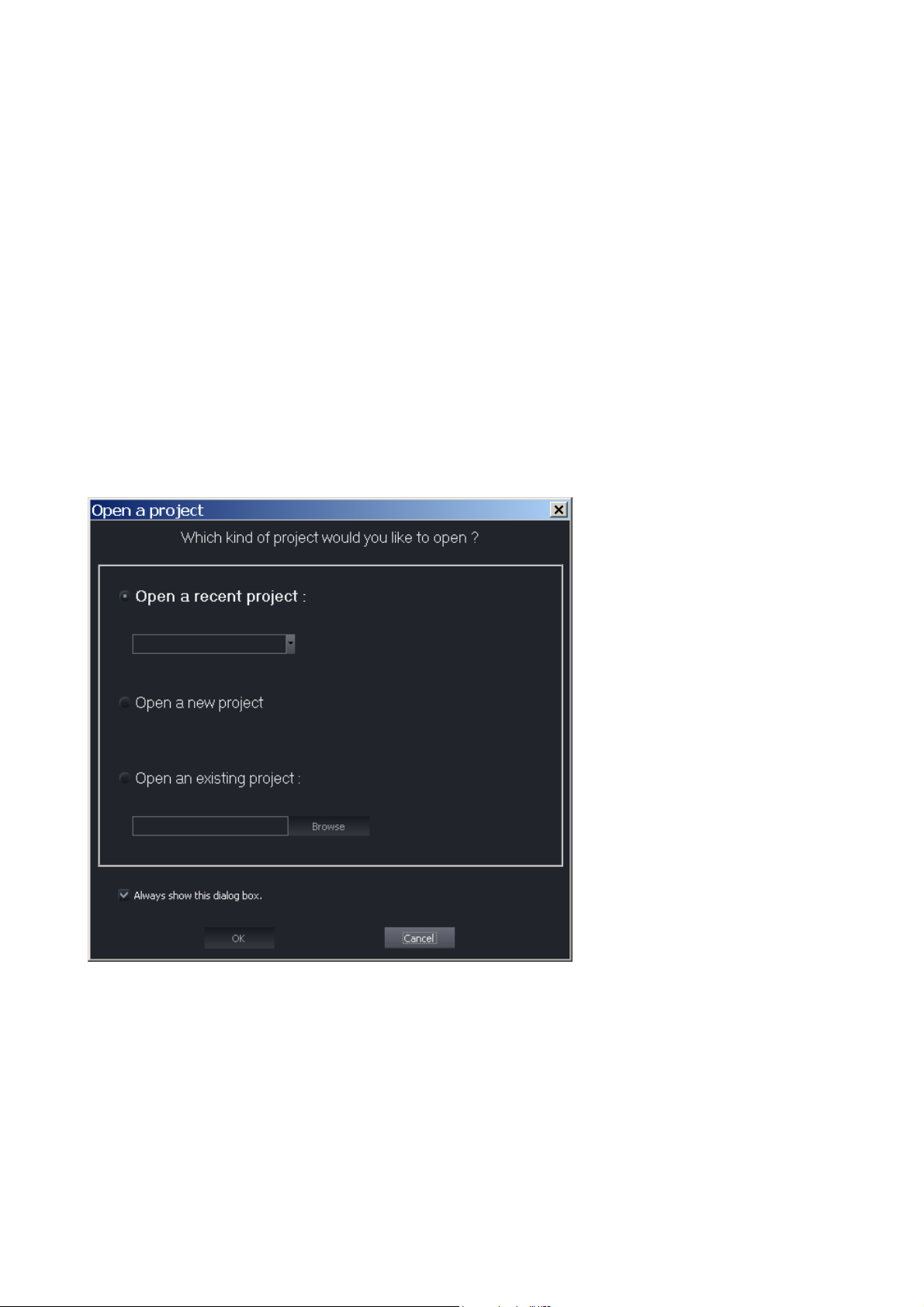
Open a project window

When you launch DxO Optics Pro for the first time, you will see the following screen:

(To avoid seeing this screen each time you launch the application, uncheck “Always show this dialog box”)

‘Open a recent project’ lists the five most recent projects, for fast access to your work in progress.

‘Open a new project’ lets you start a fresh project, and prompts you to name

Page 30

DxO Optics Pro V4.2 Reference Manual

and save it, before you start your actual image enhancement session.

And lastly, ‘Open an existing project’ opens a browser window where you can locate and open an existing saved project.

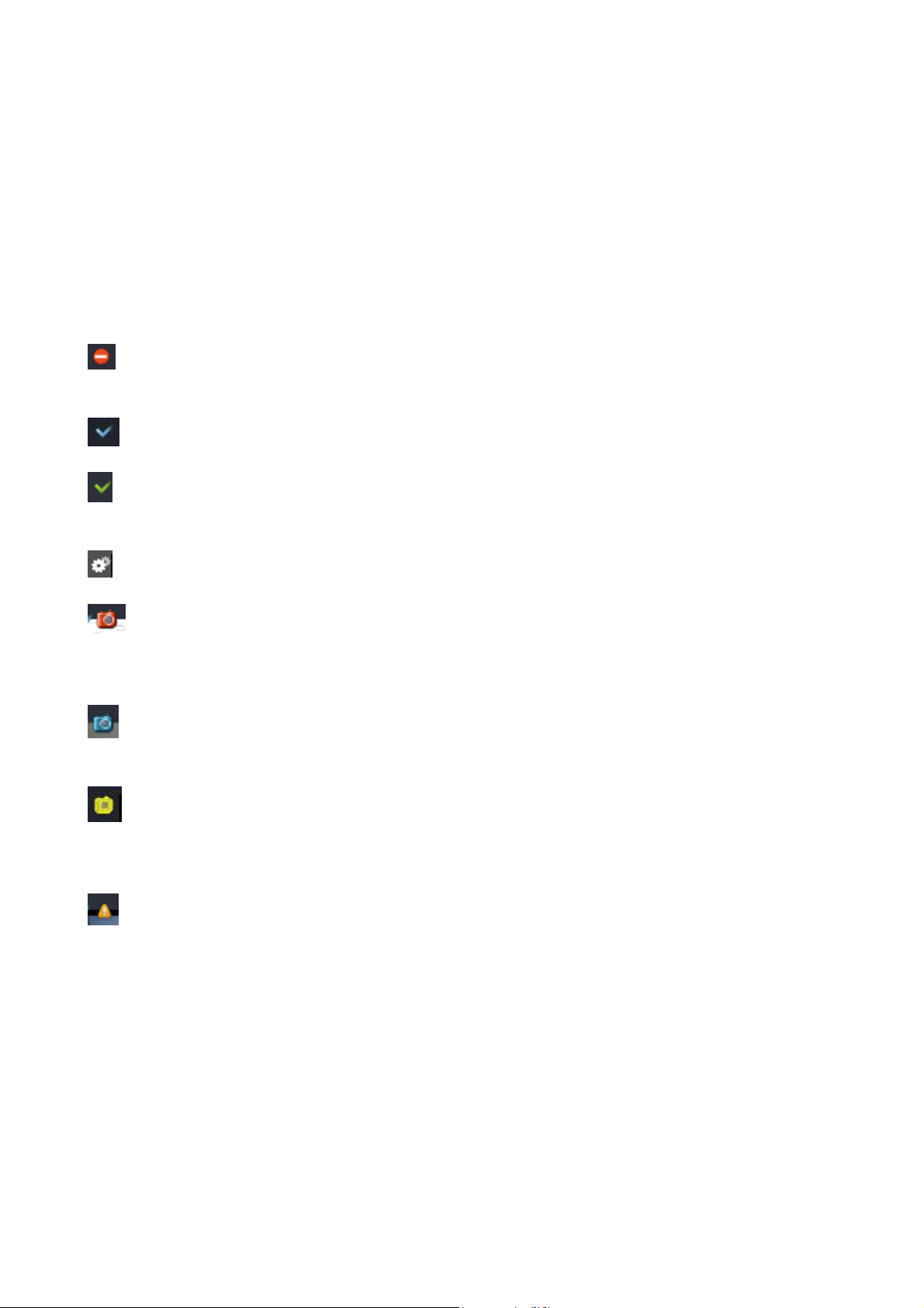
Specific icons

Once your project is open, you add images to it. In the Project pane, the thumbnail of an image can carry various icons:

: This image cannot be processed (either it’s too small, or it has

already been processed, or DxO Optics Pro cannot read its format).

: Image ready to process

: Image already processed

: Image currently under process

: This little red camera means the image is a JPEG, and no lens module is available for it (on your computer: maybe a lens module could be downloaded from DxO website).

: The blue camera means this RAW image can be processed, but

again no lens module is available on your computer.

: The yellow camera means the RAW format can be processed, the lens module is available, but the EXIF information has been modified (probably by another incompatible software).

: This orange warning sign means no focusing distance is available in the EXIF data; the image will be processed with a default infinite setting, unless you change it (in the Enhance window).

Page 31

DxO Optics Pro V4.2 Reference Manual

Chapter 10 Generic tools

Zoom

The Zoom tab, on top of the Tool Palette, shows a thumbnail of the image. The green box indicates the section of this image currently displayed in the preview on the left. The usual two buttons (bigger on the right, smaller on the left) surround a slider that can help you to fine-tune the zoom factor. Two other

Page 32

DxO Optics Pro V4.2 Reference Manual

buttons propose a shortcut for the full view (“Fit”) and the 100% view, when every pixel of the picture is represented by one pixel of your screen.

It’s important not to forget that the normal preview image only shows an approximation of some of the corrections to be applied (White Balance, Exposure, rough Demosaicing, Distortion, Vignetting, Tone Curve, Lighting, Hue/Saturation/Luminance), whilst other key corrections like noise reduction, lateral chromatic aberration, true demosaicing, and sharpness processing are not always previewed; especially when displaying at zoom factors less than 75%. While editing the Settings, you will probably frequently zoom in to check the effects of your corrections, and zoom out to control the global image. Note that a mouse thumbwheel (when available) will act as a zoom in/out control, within the same limits as the standard zoom controls.

Histogram

You’ll no doubt already be familiar with the histogram display — it’s a graph showing the number of pixels for each tonal value in the three color channels, with black on the left and white on the right. You’ll almost certainly find it very helpful to keep the Histogram tab open while you’re working with the other tools, since it very often gives you a good idea of exactly what’s going on. Below the histogram graph itself are three buttons [ ] Highlight clipping / [ ] No clipping / [ ] Shadow clipping. These activate the special

clipping display

described later.

EXIF Editor

The EXIF editor tab enables you enter and/or modify Artist and Copyright data for the currently selected image(s).

Presets

This is where you can save (and manage) your presets for subsequent reuse on other images. Saving presets of the current image permits you to define a new Preset document that you can name as you like and which will be available in the drop-down list under the Presets tab in your future Projects. It will also be available under the “Select” tab, when you import images with an associated Preset.

Presets are a powerful feature of DxO Optics Pro. Basically, all the settings you’ve carefully prepared associated with a certain image can be saved as a preset, which can then be applied to other images—most often, similar images from a same batch. More powerful still, you can choose which parameters to include or not in your preset, and manually override any preset settings at any time. So you can very speedily apply your preferred global settings to achieve the kind of ‘look’ you want, and then work on each image individually to finetune some corrections and adjustments that perhaps need to be done on an

Page 33

DxO Optics Pro V4.2 Reference Manual

image-by-image basis. It’s probably good practice to start off by saving most of your settings as presets, in case you want to apply similar settings again later to other images, as it is much less work than to laboriously go through trying to reproduce settings you’ve used before. It’s worth pointing out here that all your settings are saved in a ‘side-car file’ alongside each of your original image files, so if at any time you return to an image, it is possible to find out what settings were last used to process it.

At start-up, there is a list of any available existing presets, and also below it five buttons, only the left-hand one of which is available right away: Create preset. This enables you to save the current preset, and once you have a selection of presets saved, you can Copy or Delete them.

The two larger, right-hand buttons enable you to Edit the name of a preset and enter a brief description of it, and also, to apply a selected preset to the currently selected image(s).

Page 34

DxO Optics Pro V4.2 Reference Manual

Chapter 11 DxO Optics tools

Correction tabs

At start-up, all the correction tools appear as tabs stacked in the correction palette. When you left-click once on a tab, it turns bold and the relevant panel opens. As each correction panel is self-contained and independent, you will usually find it best to close each panel as you finish with it before opening the next, to avoid screen clutter. A scroll bar on the right enables you to move up and down in the palette to gain access to tabs that might not be visible, depending on the size of your preview pane.

Note that the entire palette of all tool/correction panels is now headed ‘Enhance’ and can be moved around the screen as an entity

Let’s now go through all the correction panels one by one, in the order they appear in the palette.

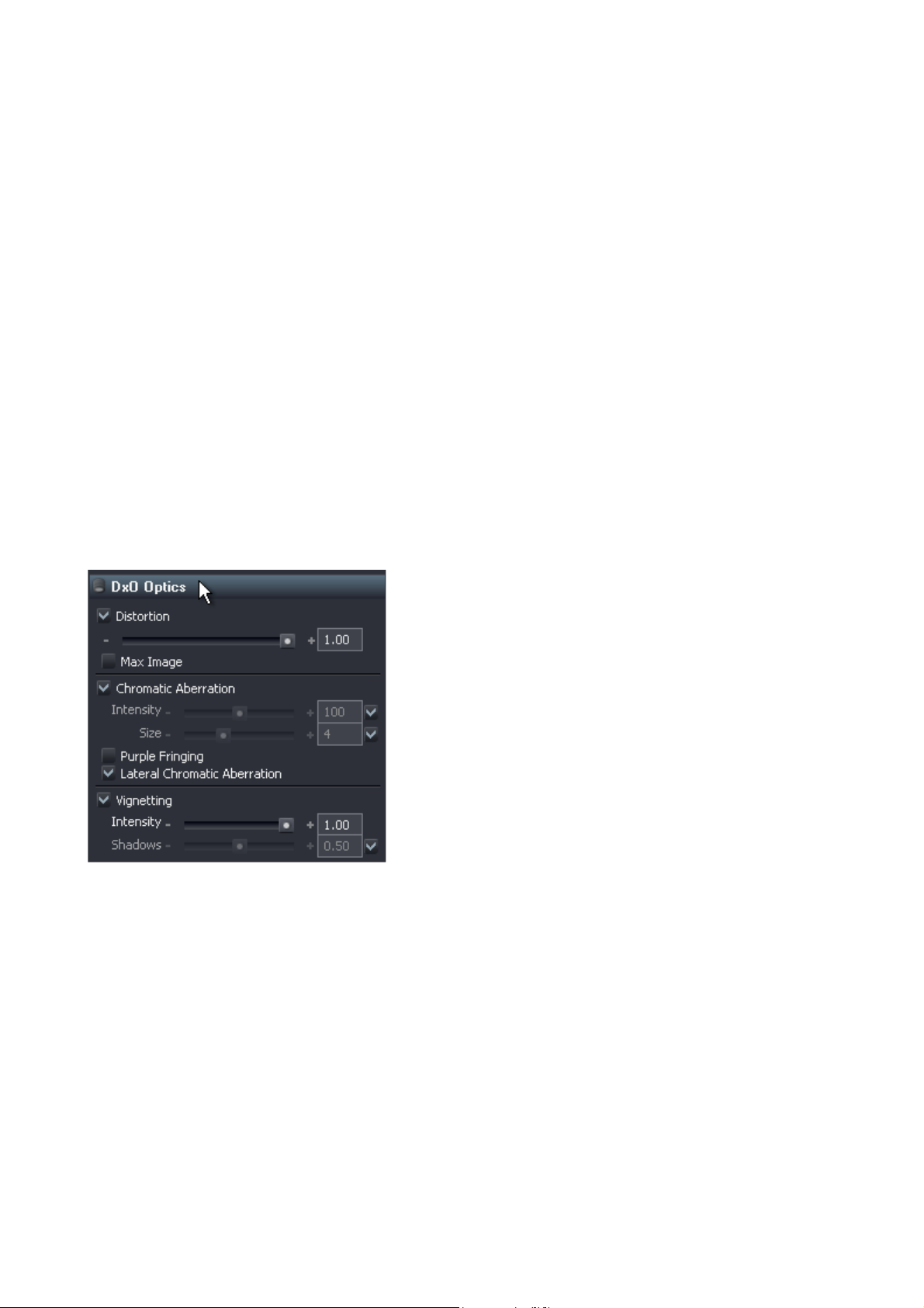
DxO Optics

There are four corrections under this tab. Note that certain of these will only be available if the appropriate lens correction module is loaded; where this is not the case, some of the corrections will appear grayed-out and be disabled.

Distortion

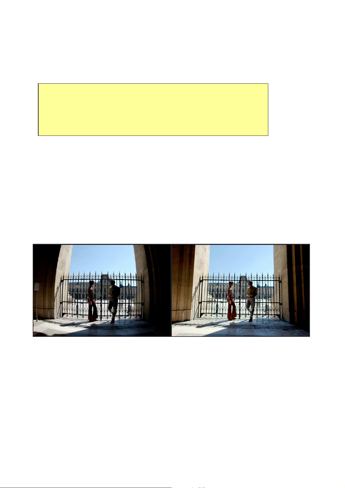
There is a check box to enable this correction, and if the check box is unchecked (correction disabled), the correction will remain grayed out. Geometric distortion may be pincushion, barrel — or even for some lenses a mixture of the two! In each case, the analytical measurements carried out by DxO Labs make it possible to correct the distortion in such a way that straight

Page 35

DxO Optics Pro V4.2 Reference Manual

lines in the original scene are correctly reproduced as straight lines in the photo. The Distortion tab has just one slider for the degree of distortion correction; the range is 0 to 100 %. The default setting is 100 %, and you should only depart from this in special circumstances—either to avoid cropping of important detail near edges, or for creative reasons.

TIP

Distortion correction involves a non-linear change in the magnification, which produces curved edges to the image and empty black spaces. To restore clean, straight edges and maintain the image’s original aspect ratio, some cropping of the image is inevitable; at very wide-angle (and especially with fish-eyes) this may be quite significant, so remember to make allowance for this when framing such shots.

There is a check box to enable or disable Max. image. Normally, during distortion correction, the corrected image is re-cropped back to the original aspect ratio; in certain cases, this may mean that the image is cropped tighter than is strictly necessary. Using Max. image releases this constraint on the aspect ratio, so the cropping is just the bare minimum required to straighten the edges of the image. You are then free to crop the image manually to suit your taste or requirements.

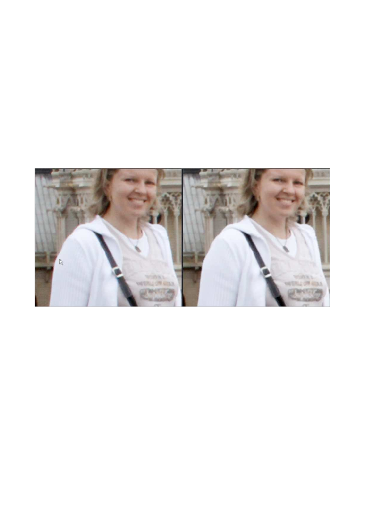
Chromatic aberration

There are two controls for chromatic aberration; to the right of them are the usual check boxes for automatic setting, which have to be unchecked to enable the manual controls. The first slider / edit box, with a range from 0 to 200 %, adjusts the correction intensity for all types of chromatic aberration—it basically affects tiny colored transitions, which may generally be assumed to

Page 36

DxO Optics Pro V4.2 Reference Manual

be the result of aberration rather than actual picture content. The second, with a range from 0 to 12 in arbitrary units, adjusts the ‘size’ of the purple fringe that will be suppressed — this basically affects the way DxO Optics Pro decides what is considered to be chromatic aberration that needs correcting and what is wanted picture content.

The Purple fringing correction just has a check box to enable or disable it — note that overall Chromatic aberration correction must be enabled in order for Purple fringing to become available.

There is also a check box to enable Lateral chromatic aberration; note that this correction depends on the presence of the correct DxO Correction Module, otherwise it will be grayed out and unavailable.

Vignetting

Again here, there is a check box to enable this correction; note that this correction also depends on the presence of the correct DxO Correction Module, otherwise it will be grayed out and unavailable.

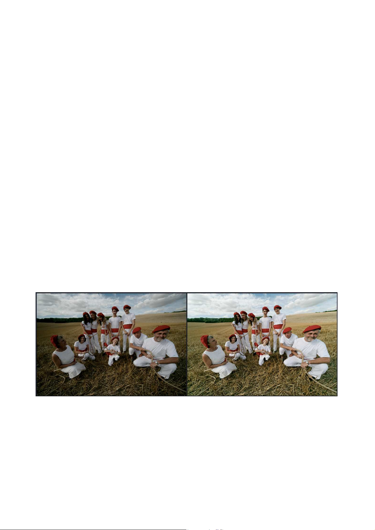
Vignetting correction takes place in two steps, both of which can be fine-tuned. First, from the lens data, focal length and aperture setting, the DxO Correction Module computes the attenuation factor for every pixel in the image, and each pixel’s RGB value is multiplied by the inverse of this factor. The correction intensity slider (range 0–100 %) allows you to decide how much of the vignetting should be removed from the whole image, independent of image content—in other words, all pixels will be multiplied by the scaled factor applicable to their position in the image field.

Page 37

DxO Optics Pro V4.2 Reference Manual

Second, a filter is applied to avoid clipping in bright areas and noise increase in dark areas. This is done by limiting the value by which a pixel can be multiplied, depending on its luminance. The effect of this filter will be different, depending on image content. The Shadows/Highlight slider lets you fine-tune this second step, so as to give preference to preserving shadow and/or highlight areas; the range is Off – 100%. As usual, the normally-checked ‘Auto’ box must be unchecked in order to enable the manual control. If you want full correction of vignetting, you can set the value to 0 (Off).

Shadow/highlight preservation restricts the amount of exposure correction applied by the vignetting corrector at both ends of the tonal range, so as to avoid either crushing in the shadows, or clipping in the highlights. So, for example, if you want to limit the luminance increase (which may reveal unwanted noise) in rather dark image corners because you shot at high ISO, shadow preservation limits the degree of correction being applied. Likewise, because of the vignetting, the camera may have incorrectly exposed a cloud in the sky; the highlight preservation filter allows you apply as much vignetting correction as possible, while still retaining wanted highlight detail.

We recommend you do not depart from the default 100 %, as the shadows preservation slider is often more effective than the correction intensity slider in preventing the undesirable effects of vignetting correction.

Note that only vignetting caused by the lens or sensor are corrected. Mechanical vignetting, caused for example by too narrow a lens shade, cannot be corrected.

Values missing

For various reasons, certain images may be missing some elements from the EXIF data, or certain cameras may not store all the data correctly. As a result, certain of the corrections (distortion, lateral chromatic aberration, lens

Page 38

DxO Optics Pro V4.2 Reference Manual

softness) that rely on this data may not be able to be applied at optimum accuracy.

When an image is selected for which this is the case, its thumbnail is marked with a “!”, and a matching new button and tab appear in the corrections palette, giving you the opportunity to fill in the missing information. When you open this panel, you will be invited to enter any one or more of the following items of information.

Focusing distance

Certain lens correction modules need focusing distance information to optimize optical corrections. Some cameras do not store the focusing distance in the EXIF data; if this is the case, the focusing distance panel will be displayed, and you should manually enter the focusing distance used for the shot, as accurately as you are able to. A check box is provided to enable the input, and a combo box allows you to select various distance ranges, while within each range the slider lets you set the distance precisely, or alternatively, enter the figures in the edit box to the right. Do note that the slider may allow you to enter a focusing distance that is not actually covered by your lens; in this case, DxO will use the minimum focusing distance applicable for your lens. Note that the units for focusing distance (feet & inches or meters) can be changed in the ‘General’ tab under the ‘Preferences’ menu, accessible via the Edit pull-down.

Focal length

Likewise, in order to optimize optical corrections, a small number of zoom lens correction modules need more precise focal length information over certain specific parts of their range than is available from the camera’s EXIF file. If this is the case, the focal length panel will be displayed, with a check box to enable the input and you should manually enter the focal length the lens was set at for the shot, as accurately as you are able to. The slider lets you set the distance precisely and will be calibrated for the range of focal lengths across which ambiguity exists for the particular lens in question. Alternatively, you can enter the figures in the edit box to the right.

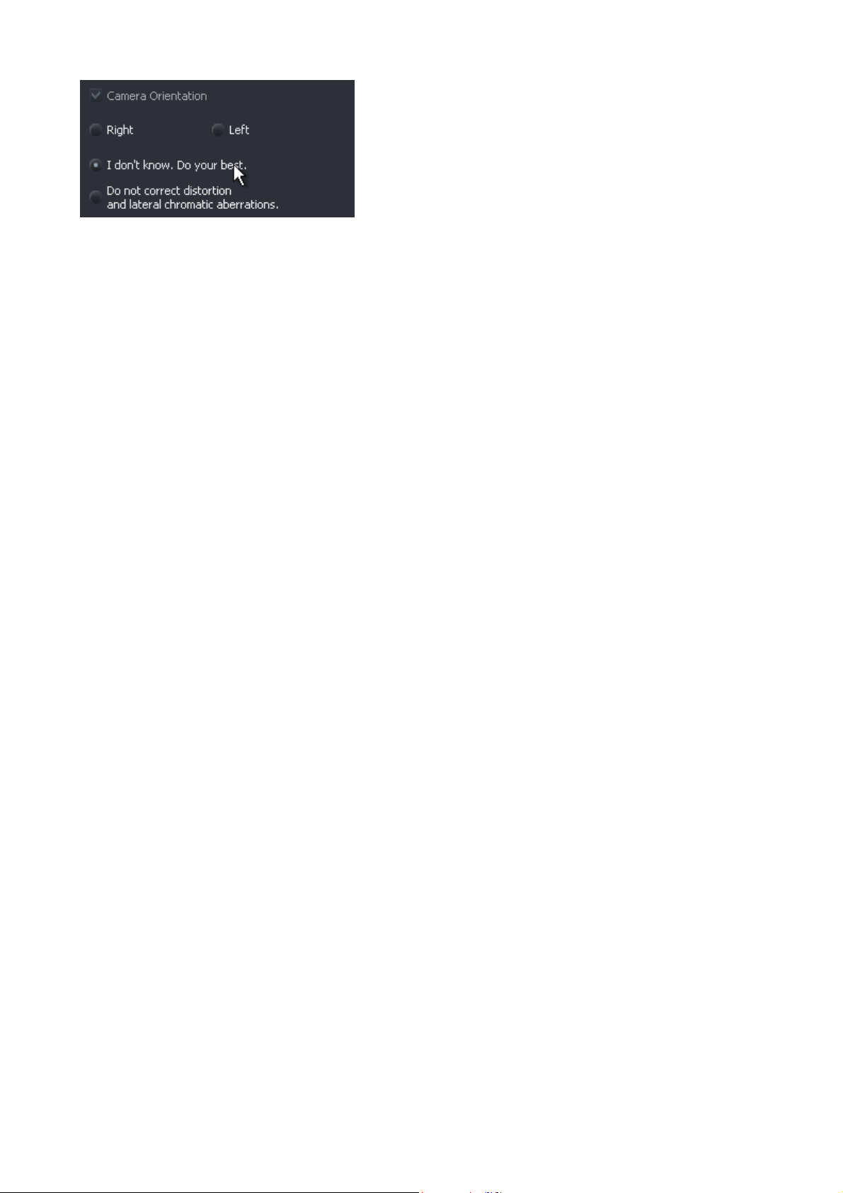
Camera orientation

Although we recommend you always use DxO Optics Pro to rotate your image automatically using the information from the EXIF orientation tag, you may have images that have been already rotated. In this case, and in this case only, the Camera orientation panel appears; it will never appear if DxO Optics Pro rotates your images automatically.

Page 39

DxO Optics Pro V4.2 Reference Manual

It allows you to specify in which orientation the shot was taken. You have three options. The first is to indicate which way the camera was turned when the image was taken (to the right or to the left). The second option is to select “I don’t know. Do your best.”, in which case DxO Optics Pro will apply a default. In the extremely unlikely event of the results proving unacceptable, as a last resort you can click the third “Do not correct distortion and lateral chromatic aberration” button.

Page 40

DxO Optics Pro V4.2 Reference Manual

Chapter 12 Sharpness tools

Sharpness

DxO can correct only for certain kinds of softness—the lens + camera combination’s inherent inability to reproduce fine detail (commonly referred to as “optical blur”). Other kinds of softness caused by inaccurate focusing, insufficient depth of field or motion blur, for example, cannot be corrected.

Remember that these corrections will not be visible in the main preview image below 75%: use the Zoom tool.

DxO Lens Softness

This forms part of Optics Pro’s optical corrections, and as such, is lens- / bodydependent. As a result, this panel will only be enabled (i.e. its title bar highlighted) for images for which the appropriate correction module is installed. Here again, there is a check box to enable this correction.

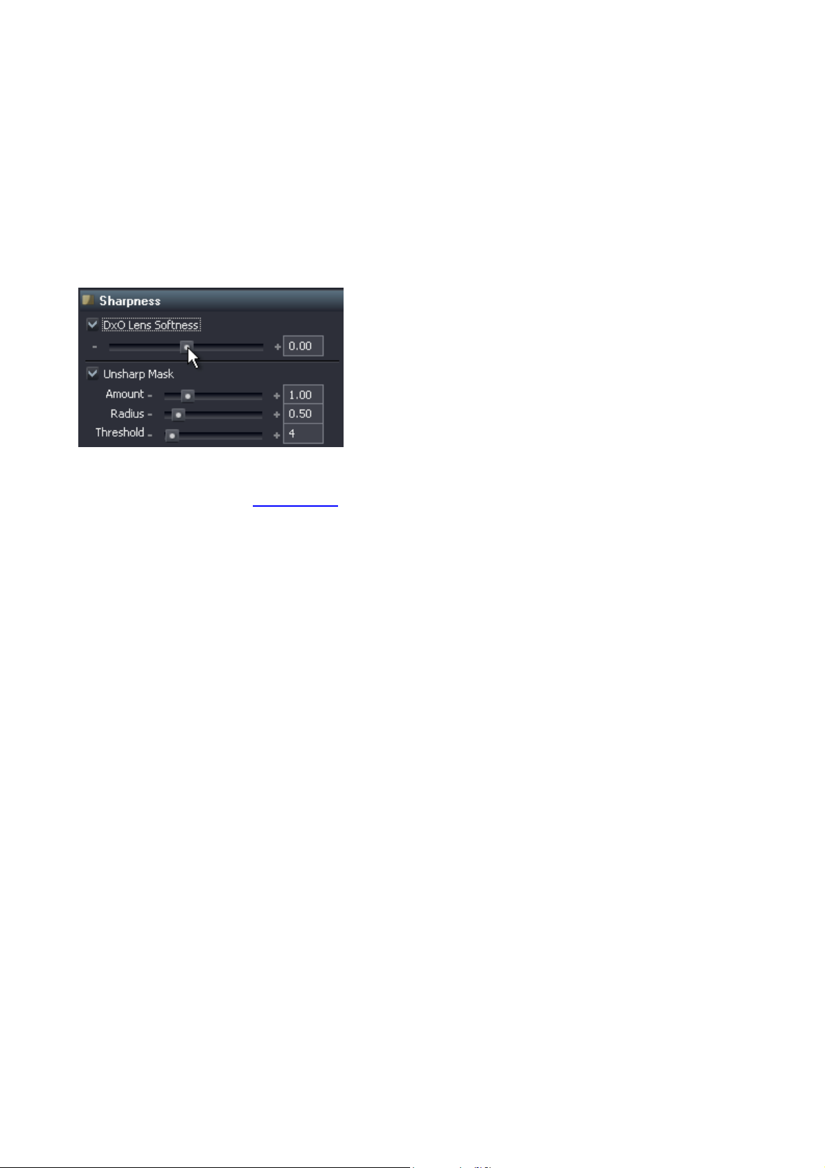
The DxO Lens Softness slider allows you to manually set the overall level of sharpness required for a particular usage. Remember that this tool intends to reach an identical level of sharpness for the entire image: it will automatically apply a stronger correction on the weak areas.

The sharpness level you choose to apply will of course depend on questions like personal taste, final resolution and type of output (print, web, etc).

The slider / edit box range is in arbitrary units from –2.0 to +2.0, from Softer to Sharper, with a default setting of 0. Moving the slider to the left or entering negative values will give a softer, smoother image, while moving it to the right or entering positive values will give a sharper image.

The value –1 is the equivalent of “Gaussian Blur” in Adobe Photoshop®. The value +1 is not a simple unsharp mask. The sharpening applied in DxO Optics Pro is intelligent, in that it depends on the image content. Areas with noise are sharpened less than areas containing detail. For each area in the image, the amount of sharpening will also depend, for example, on the ISO; less sharpening is automatically applied at high ISO than low ISO, to avoid increasing the noise in the image.

Page 41

DxO Optics Pro V4.2 Reference Manual

Note that because this sharpness correction is specifically tailored for your camera’s optics, and may well vary across the image field (to allow for lens performance shortcomings), it is usually preferable to perform as much of your sharpening as possible using this Lens Softness correction. This allows lighter use of the Unsharp Mask (USM), which although a sophisticated and adaptive tool, is a nonetheless a more generalized process. Of course, for images where the appropriate DxO Correction Module is not installed, all sharpening has to be done in the USM.

Unsharp Mask

Once again here, there is a check box to enable this correction, and if the check box is unchecked (correction disabled), the title bar and controls will be grayed out. The Amount slider / edit box obviously sets the degree of sharpening correction applied, with a range from 0 to 5.00. The Radius slider / edit box has a range in arbitrary units from 0.10 to 5.00. This control affects the fineness of the correction zone surrounding image detail; low values give very subtle correction, whilst over-use of high values can lead to the formation of haloes. The Threshold slider / edit box has a range from 0 to 255, and adjusts how far up the tonal range sharpness correction commences. To avoid noise increase in lowlights, which may not contain much wanted detail, the threshold can be raised so that sharpness correction starts at a higher gray level.

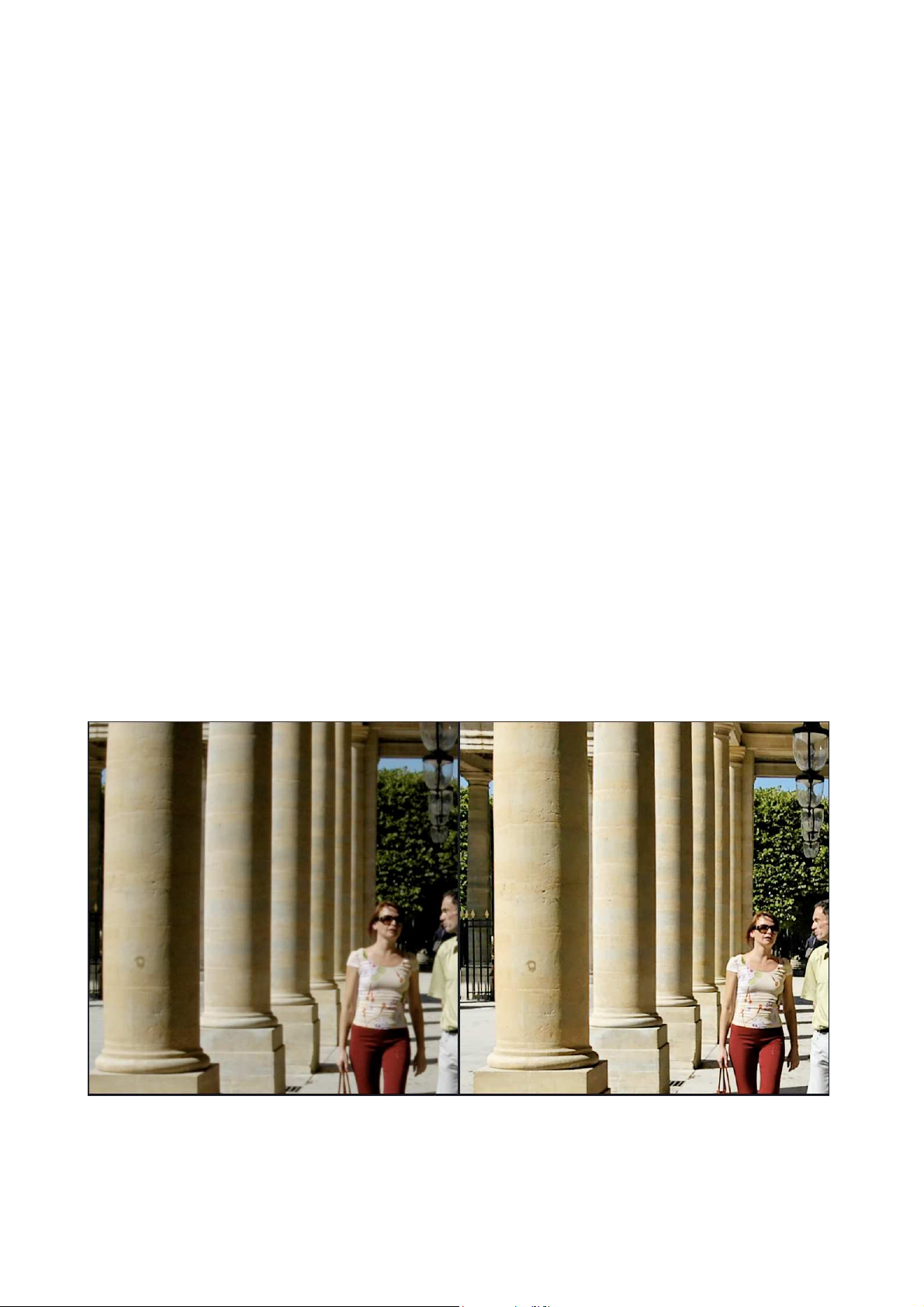
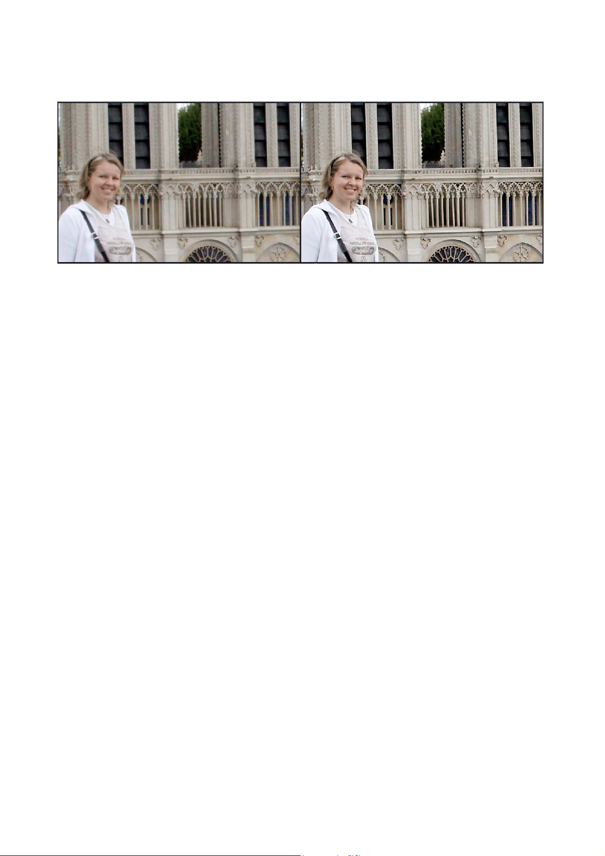
Take a look at these images to see the effect of these controls:

DxO Lens Softness

Page 42

DxO Optics Pro V4.2 Reference Manual

Unsharp Mask

Page 43

DxO Optics Pro V4.2 Reference Manual

Chapter 13 DxO Noise tools

DxO Noise tab

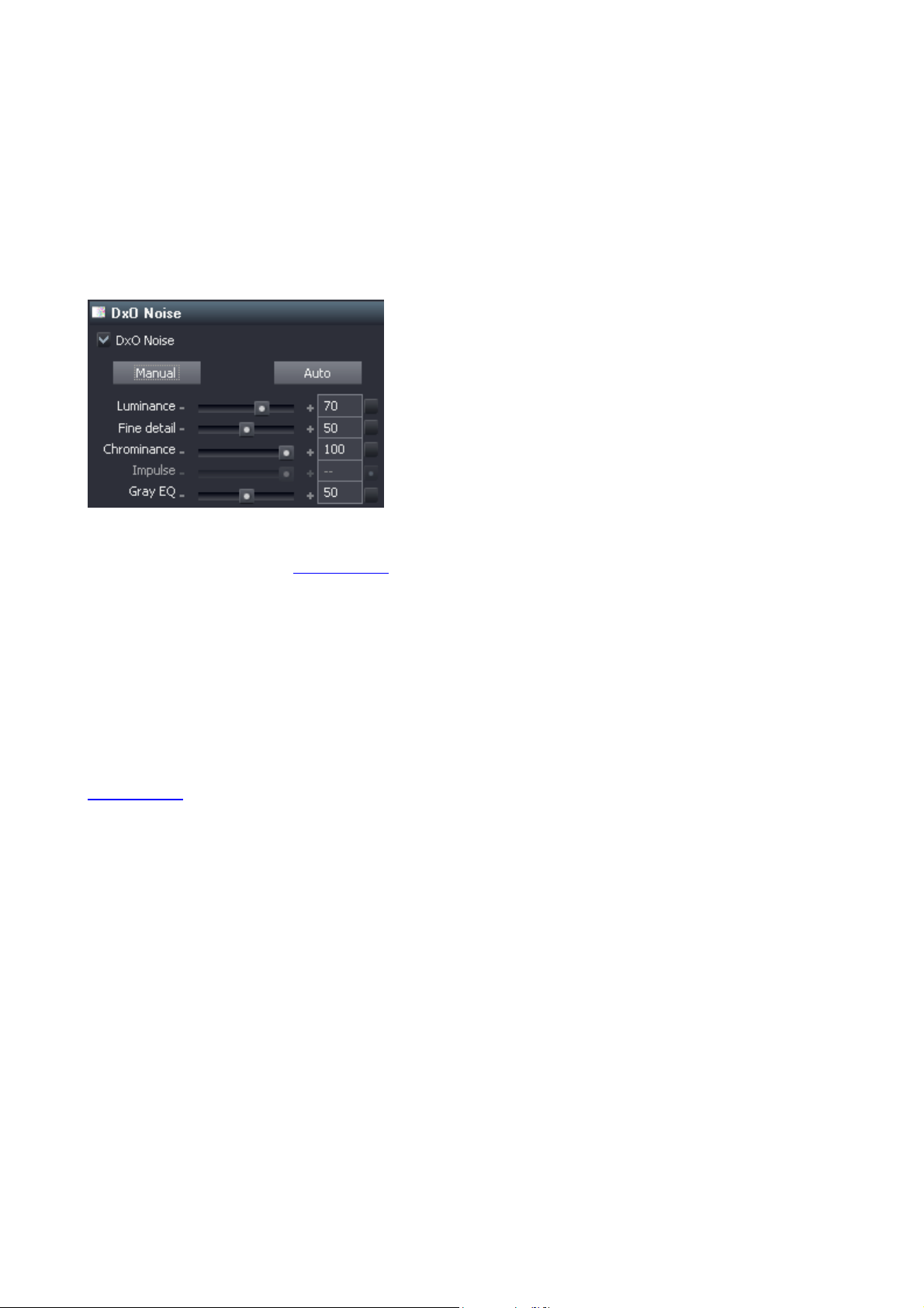
DxO Noise is a calibrated correction, in other words, the correction algorithm is specifically tailored for each camera, and so this correction will only be performed for images from cameras that have been calibrated by DxO.

Remember that these corrections will not be visible in the main preview image, but only by using the Zoom tool.

Once again here, there is a check box to enable this correction, and if the check box is unchecked (correction disabled), the entire panel will be grayed out. All five controls under this tab have individual ‘Auto’ boxes to their right that have to be unchecked in order to enable the manual controls; there are Uncheck all (= all manual) and Check all (= all automatic) buttons at the top that can be used to uncheck / check all the controls at the same time.

In order to judge the effect of your noise adjustments, it is essential to use the

Zoom tool, which gives an accurate preview of final image quality. Choose an

area of your image where you can best assess the noise to make your adjustments, and then if necessary move the zoom area around in order to examine other critical areas.

The degree of Luminance noise correction can be set using the slider / edit box, with a range from 0 to 100 %. Although DxO Optics Pro’s luminance noise reduction is intelligent and discreet, it is still advisable to use the minimum amount of correction that produces acceptable results, to avoid any danger of unwanted effects on fine detail.

To minimize such effects, there is a ‘Fine detail’ slider / edit box, with a range from 0 to 100 %. The default value is 0, but you can increase this setting in situations where you might need to restore some of the fine detail that can be attenuated during strong luminance noise reduction, creating an undesirable ‘plastic’ or waxwork look.

Page 44

DxO Optics Pro V4.2 Reference Manual

The degree of Chrominance noise correction can be set using the slider / edit box, with a range from 0 to 100 %. This is useful for reducing or eliminating colored noise—to which the eye is particularly sensitive—and you can usually safely use quite high settings with little risk of unwanted side-effects.

Impulse noise correction can be added using the slider / edit box, again with a range from 0 to 100 %. It offers very effective reduction of impulse-type noise (which only affects certain specific cameras), but should be used judiciously, because of the slightly greater risk of its having a visible effect on wanted picture detail. Note that when processing Raw images this control is not available (it will be grayed out), as this correction is applied automatically as part of the Raw conversion process.

The Gray equalizer slider / box has a range from 0 to 100 %. This makes it possible to ‘clean up’ unwanted colored noise from midtones, and has the effect of slightly de-saturating neutral tones around mid-gray, to minimize spurious color effects in these sensitive areas. You will probably be able to leave it at the default setting, unless you notice the effect it can have of desaturating certain pastel tones.

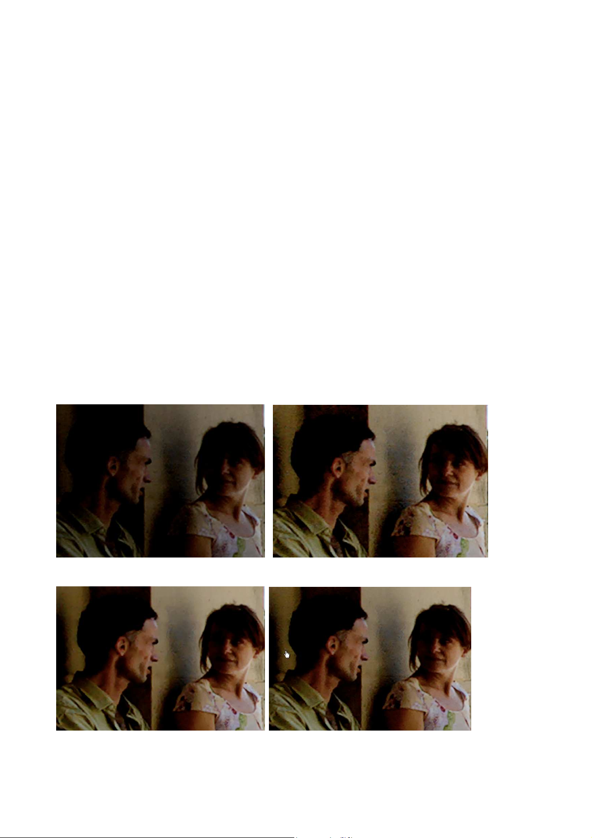
Look at the pictures below, which illustrate the effect of this noise reduction, particularly visible in the shadow areas.

Original image Lighting activated

DxO Noise activated Fine details

Page 45

DxO Optics Pro V4.2 Reference Manual

Chapter 14 White balance and Exposure

Under this tab you’ll find two panels for this group of related correction controls:

RAW White Balance / JPEG White Balance

Note that there are two different groups of controls, depending on whether you want to process a raw or RGB (i.e. JPEG/TIFF) format image. In the case of raw images, true white balance adjustment is possible, whereas in processing the other image formats, the white balance adjustment is achieved slightly differently. For a given image of either type, the unwanted group of controls will be grayed-out and disabled.

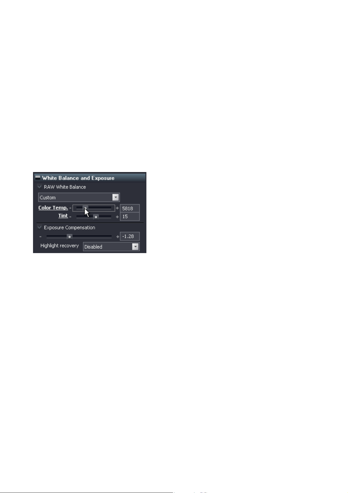
At the top of the RAW White Balance panel is a combo box, offering ‘As shot’ (i.e. uses the values read from the image file’s EXIF header), a series of presets for ‘standard’ lighting conditions (Daylight / Cloudy / Tungsten / Fluorescent / Flash / Shade), and a ‘Manual temp.’ position that allows use of the sliders (any adjustment to the sliders automatically selects an ‘As shot (Custom)’ setting).

The top slider adjusts the color temperature—basically, it swings the balance of the red and blue channels, whilst leaving the green untouched. Moving the slider to the right increases the color temperature, moving it to the left decreases it. The same result can be achieved by typing in a figure for the color temperature and pressing ‘Enter’. The range is from 2,000 K to 20,000 K.

Note that the effect on the image is to make it warmer with increasing color temperature, and cooler with decreasing; although this might at first appear counter-intuitive, we need to remember that this is correcting the color balance as if the picture had been shot with this color temperature lighting in the first place. Imagine, for example, that a picture has been taken by tungsten artificial light, but with the camera accidentally set to ‘daylight’; the resulting image will appear too orange. Moving the slider to the left, towards a

Page 46

DxO Optics Pro V4.2 Reference Manual

lower K value more appropriate for the artificial light actually used, will cool the image, correcting the orange cast.

The lower slider adjusts the ‘tint’—in this case, swinging the color balance between blue and green, leaving the red untouched. Moving the slider to the left (or entering a negative number) makes the image greener, moving it to the right or entering a positive number makes it bluer. The range runs from +100 to –100.

Let’s take a look at the operation of these two controls using some actual pictures (in this case, raw images).

Here in the middle is the picture as shot, and to the left and right, the effects of shifting the color temperature slider left and right respectively:

And here is the same picture, this time with the tint control adjusted :

At the left of the header bar is a button to activate an eye-dropper tool that lets you pick a neutral area of the image to be taken as a white reference. This should be a fairly light grey tone, but avoid clipped highlights, as the results can be very unpredictable! Clicking this button displays two preview images side by side, the left-hand one being the original image, and the right-hand

Page 47

DxO Optics Pro V4.2 Reference Manual

one showing the effect of adjusting the white balance according to the reference point chosen. Note that the eye-dropper ‘looks’ at the average of a number of screen pixels, so you should also avoid transition areas that might yield unwanted errors. Simply position the pointer over the required area, and left-click to white balance for this point; at any time, you can re-select ‘As shot’ (on ‘White balance and Exposure’ panel) in order to cancel the changes and revert to the original white balance. Immediately you click on a gray point to adjust the white balance, the combo box selection automatically changes to ‘As shot (Custom)’. The eye-dropper tool can be temporarily disabled using the Alt key (toggles); as soon as you right-click anywhere in the image, it comes back (but without changing the white balance, or if you left click, it comes back and changes the white balance at the same time).

Note that if you zoom in during this twin-image white-balance display, the eyedropper tool then prevents you from being able to move the images around with the hand tool. The way to do so is to open the Zoom tool and use the green box to move the zoom window around within the image.

TIP The way the software performs White Balance adjustment differs slightly between processing raw and RGB images (JPEG and TIFF). Using raw images allows greatest freedom of white balance adjustment, but you need to exercise care when correcting RGB files, as large amounts of correction can lead to undesirable artifacts (banding in high-key areas / posterization in shadows).

If the image selected is an already-converted RGB file, you will need to use the JPEG White balance panel. This has just a single slider to adjust the overall balance of the image—cooler to the left, warmer to the right—or an edit box to enter a color temperature value, with arbitrary units from 0–100. Extreme settings in this RGB mode need to be used with care, in order to avoid artifacts that are the result of limitations in the RGB formats themselves. As before, clicking on a gray point in the image using the

eye-dropper tool will adjust the

overall white balance so as to make this point neutral, and the selection in the combo box will change automatically, this time to ‘Click point’.

DxO’s powerful tone curve, lighting correction and noise reduction features mean you’ll be able to recover an astonishing amount of shadow detail that in conventional photography would likely have been lost. But these corrections are most effective when processing Raw images, which is why the Raw format is to be preferred whenever possible for images to be processed.

Exposure compensation

This slider works just as you might expect—moving it to the right (or entering a positive Ev number into the edit box) increases the exposure, to the left (or a negative Ev number) reduces it. The range is from +4.00 Ev to –4.00 Ev.

Page 48

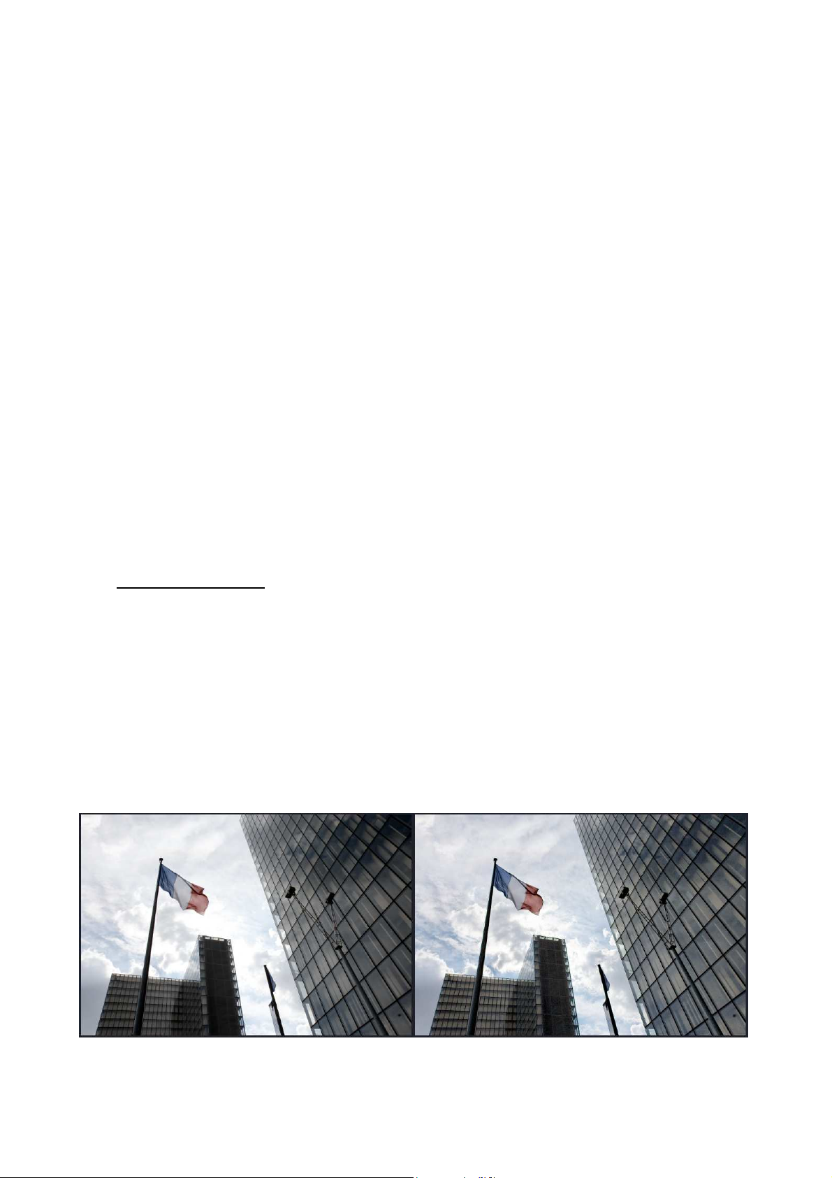
DxO Optics Pro V4.2 Reference Manual

During exposure adjustments, you may well find it helpful to use the highlight / shadow clipping display, available via the buttons beneath the Histogram display.

These displays are intended to give a temporary pictorial indication of those parts of an image that are ‘clipped’ (i.e. dark areas that have reached minimum black level or light areas that have reached maximum white level). Clicking on the ‘highlight clipping’ button displays a picture that is mainly black (= areas with no clipping), in which certain small areas will display as white (= highlights where all three color channels are at maximum) or as different colors (= only one or two color channels are at maximum). This enables you to spot at once precisely which parts of your picture are clipping, and hence make a more informed decision as to what corrections to apply.

The exact opposite is true for the shadow clipping button—in this case, the picture displayed is mainly white, with small black or colored areas indicating clipping.The middle button restores the normal display.

It’s important to note that shadow and highlight clipping displays are computed in the final output color space, and hence these displays, and any adjustments performed based on them, will be affected if the output color space is subsequently changed.

Highlight recovery

Highligh recovery is only available for raw images (it is disabled when working on an RGB [JPEG] image). A drop-down menu offers the choice of None / Slight / Medium / Strong intensities of correction.

On this image, note how checking the ‘Highlight recovery’ box produces a slight reduction in exposure and retrieves highlight detail that had appeared to be ‘lost’; this is one of the great advantages of working with raw images, since with an RGB image, once highlights are ‘blown’, there is no possibility of rescuing the lost detail.

Page 49

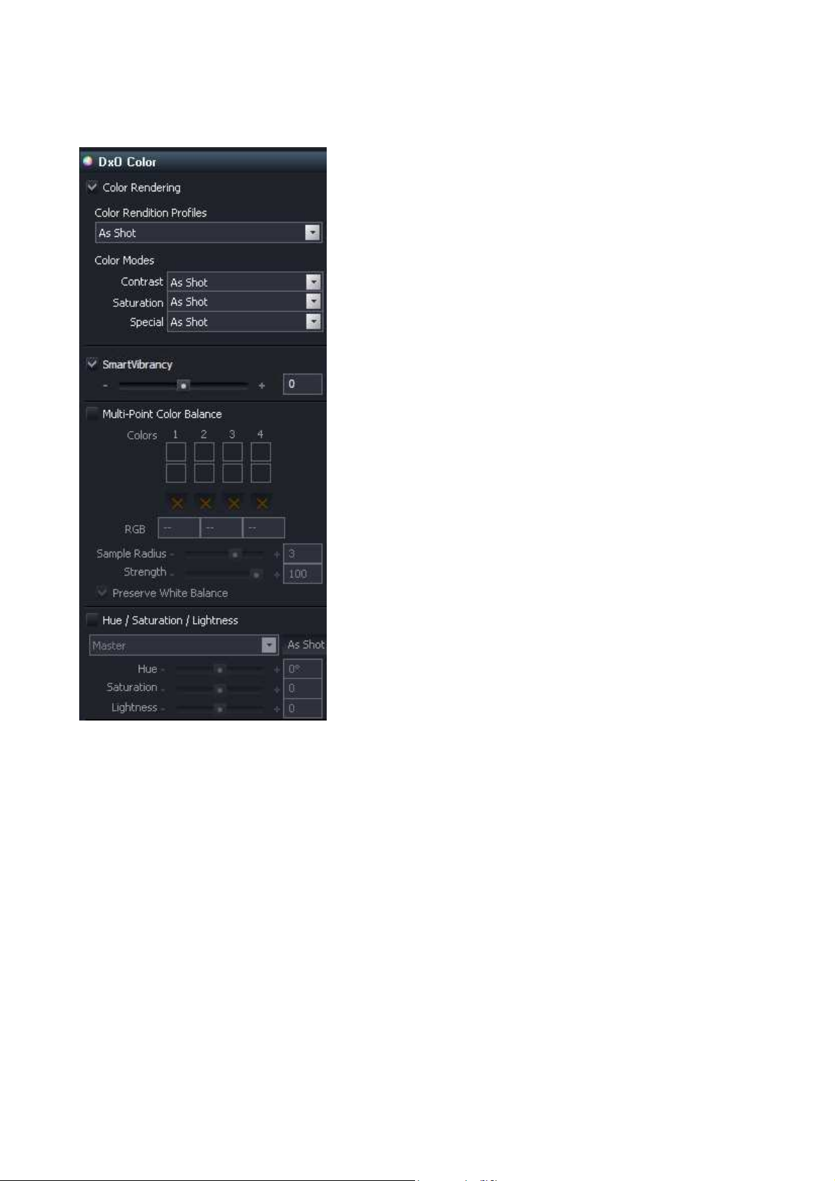
DxO Optics Pro V4.2 Reference Manual

Chapter 15 DxO Color tools

Color rendering

Color rendering lets you apply a specific look to your Raw images, starting right from the very look of specific camera bodies, referred to here as ‘color rendition profiles’. This functionality will slightly differ if you have activated the DxO FilmPack (see chapter 19). As usual, there is a check box to enable this function, and a combo box lets you choose between ‘Original’, Neutral’, and ‘Realistic’, along with specific color rendition profiles for 7 families of cameras currently supported by DxO Optics Pro. Realistic is the “flat” color rendition profile, without any interpretation, with a gamma valued at 2.2. Neutral has the same color rendition, but with a contrast slightly increased. The command « Import an ICC profile » available in the menu « Color rendition profiles » allows you to load a specific profile created from a test image, with the adjustments entitled either “Realistic” or “Linear Raw” (see the creation of profiles in Chapter 8).

Page 50

DxO Optics Pro V4.2 Reference Manual

The implication of this is far-reaching; it means you can shoot with multiple bodies from different stables, and yet always produce results with consistent color rendition. You can apply the color rendition profile of Brand X to a camera from Brand Y, so all your pictures look as if they were taken using your Brand X. Alternatively, the two more neutral settings cancel out even these tiny variations between cameras, to produce a technically precise, neutral result.

Color modes

Color modes offers you three combo boxes where you can make some preset and repeatable choices about the overall look of your image. These color modes are available for both Raw and JPEG images. Choices of high / medium-high / medium-low / low are offered for both contrast and saturation. Special offers original, two ‘style’ presets: portrait and landscape, together with black & white and sepia effects. ’Portrait’ and ‘landscape’ each apply a fairly subtle color/contrast preset that has been developed to be generally suitable for these two broad types of picture; these are extremely convenient as a quick and repeatable solution for those who do not need or wish to make individual corrections of these parameters for each individual image. As their names imply, ‘B&W’ removes all the color from the image, while ‘sepia’ tones the whole image with a pleasing sepia effect.

SmartVibrancy

Moving the slider controlling SmartVibrancy to the right will enhance the colors to make them more appealing, while avoiding undesirable side-effects. On the opposite, moving it to the left will reduce the strenght of the colors in an oversaturated image.

Multi-point color balance (MPCB)

One of the brand new features in DxO Optics Pro version 4, this offers a sophisticated way of achieving exact color matching between shots, even where a neutral color reference is missing. The system allows you to pick up to four colors and set the color you want each of these to be reproduced as, and then DxO Optics Pro will make a best-compromise calculation to adjust the color balance of the entire image — what’s more, it can do this across a whole string of images, making it is easier than ever before to match critical colors between different shots.

To use this function, you first need to click on the appropriate button

on the left-hand side of the ‘Enhance’ header bar; this will open the DxO Color correction panel and check the Multi-Point Color Balance enable box, if it isn’t already. It will also put the preview display into twin-image mode (before and after correction).

Page 51

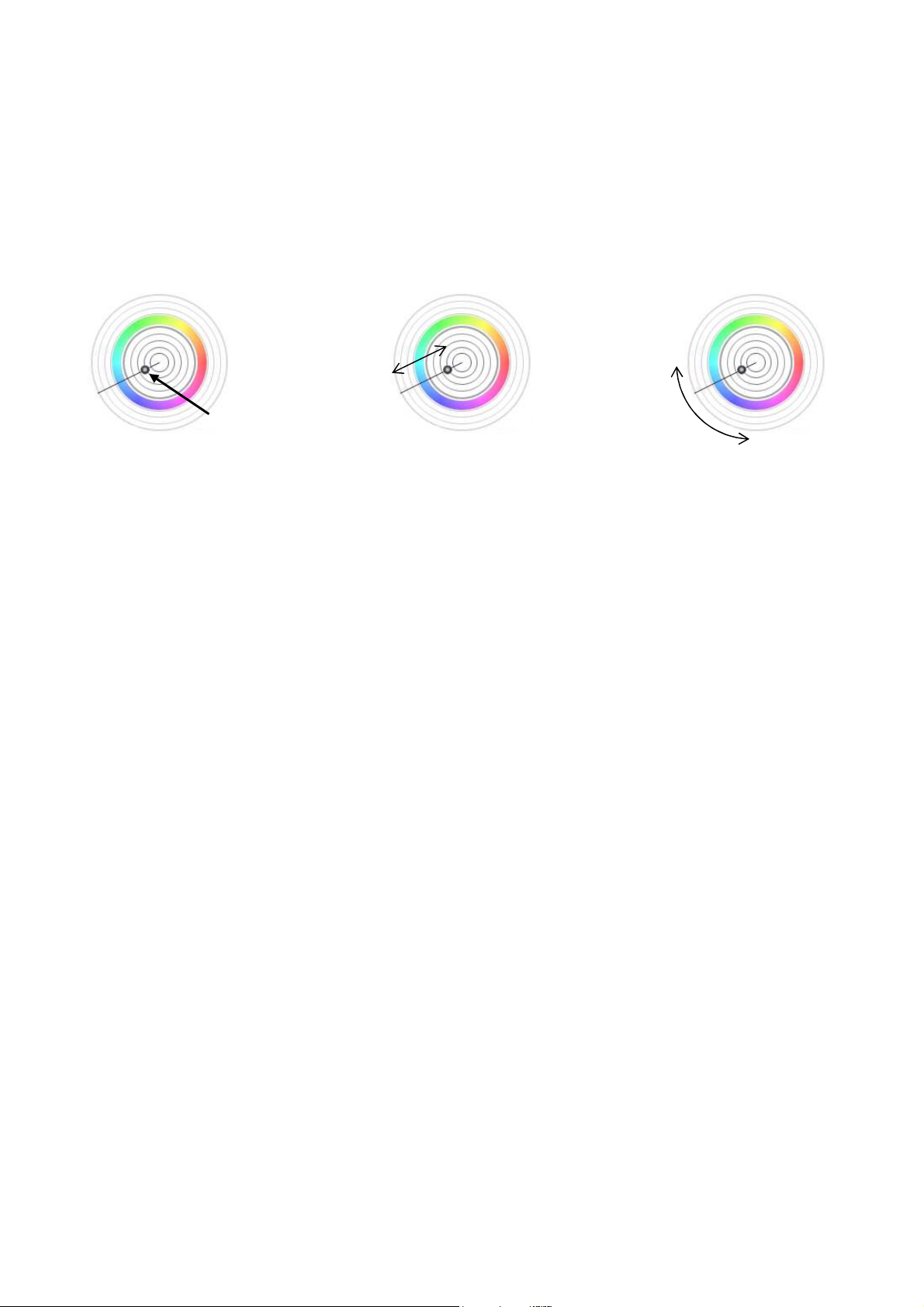
DxO Optics Pro V4.2 Reference Manual

Drag this point to

On the MPCB panel, you have four pairs of color patches labeled 1–4; these will show the color points you pick in your image, and beneath each of them there is an X to delete them. There are also corresponding Edit RGB boxes where you’ll be able to directly enter numeric red / green / blue values.

As soon as you left click on the left-hand image, you will select a color to go in the top (‘before’) color patch, and a color wheel will appear on your image, like this:

adjust slider

The centre of the color wheel corresponds to the point you have selected, its size (from 1 to 4 pixels) set by the ‘Sample radius’ slider / edit box on the MPCB panel.

Now you can use the mouse to drag the cursor in order to set the color you would like this first point to reproduce as. Dragging the cursor in and out on the radius reduces or increases the saturation, and dragging it in an angular direction changes the hue. The saturation is displayed alongside the color wheel as a value from 0 to 100 %. If you right-click on the cursor, a drop down offers you ‘No lock / Lock hue / Lock saturation’—checking the appropriate one will enable you to lock either hue or saturation to stop them moving while you adjust the alternate parameter, or else allow you to unlock both together. You can also temporarily lock the hue by holding down the Ctrl key as you drag with the mouse, or the saturation by holding down the Shift key.

The result of your color adjustment will be previewed in the right-hand ‘after adjustment’ image, and the new color (‘after’) will be shown in the lower patch.

If you want to select further points for balancing, you can just click again; as you do so, the previous color wheel will collapse to a small circle with its number beside it. You can revisit an earlier color point at any moment by clicking right in the centre of it, and you can move it around by grabbing it at any point other than the cursor itself and just dragging it to where you want it. You can delete any color point at any time just by clicking on the X button beneath its color patches.

Also on the MPCB panel are two sliders / edit boxes for Sample radius (range 1 to 4 pixels) which sets the size of the point around the cursor that is averaged,

Page 52

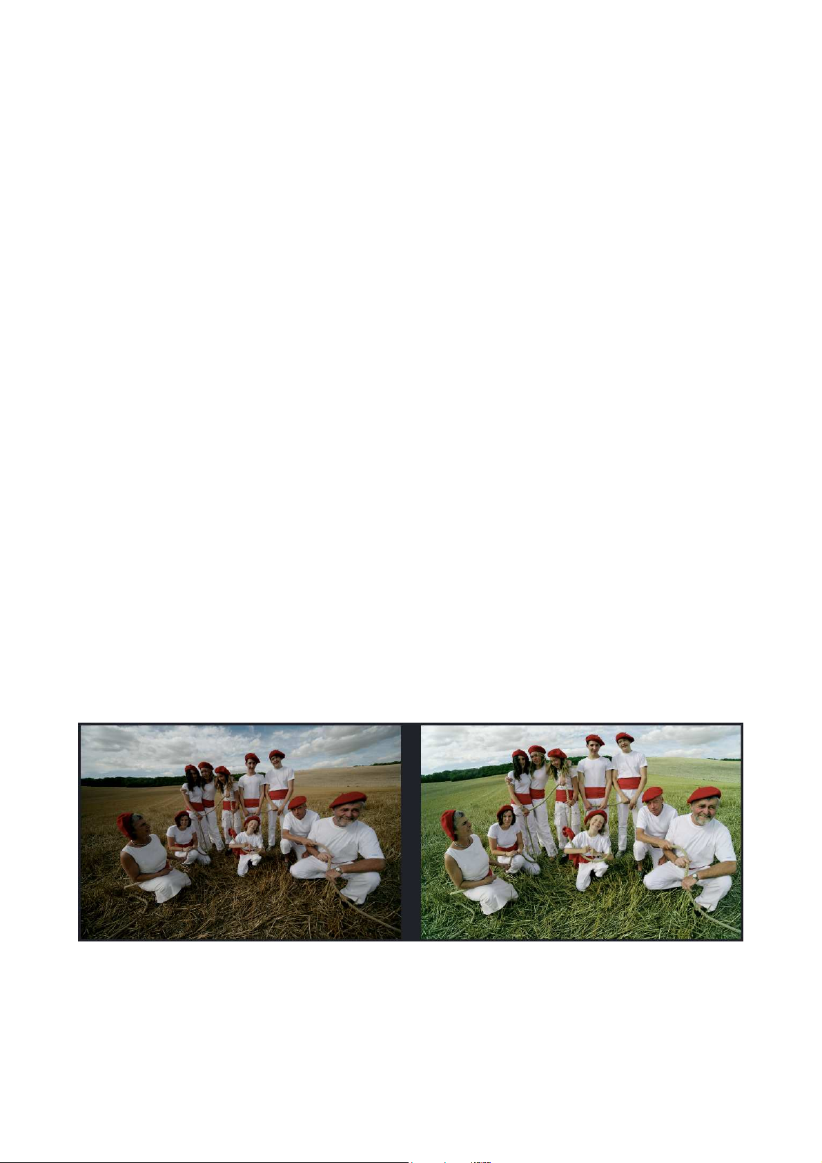
DxO Optics Pro V4.2 Reference Manual

and Strength (0–100 %), which enables you to adjust the flexibility around the clicked point—and a check box for ‘Preserve white balance’. From the points you set, DxO Optics Pro calculates the color adjustments that need to be made to achieve the balance you require. If there is a conflict between the points you have set, then it will make the best compromise it can between them all. If you check the box to enable ‘Preserve white balance’, then DxO Optics Pro will calculate the compromises in such a way as to maintain the neutrality of the image as far as possible. With this mode enabled, attempting to force a color cast onto an originally neutral point is clearly likely to produce unpredictable results

Note: the MPCB and HSL color adjustment modes are mutually exclusive; so if you have made adjustments in one mode, and then attempt to change over and make adjustments in the other, you will receive a warning message saying that your earlier settings will be lost, and asking you to confirm that you want to continue.

Hue / Saturation / Lightness

As usual, this panel has a check box to enable the correction, and if unchecked (correction disabled), all the controls will be grayed out.

Hue, saturation and lightness can all be adjusted for the master channel, and also separately for each of the three primary (Red, Green, Blue) and three secondary (Yellow, Cyan, Magenta) color axes, as selected in the combo box.

As usual, the Hue slider can be moved to the right or left to change the hue, or a positive or negative figure can be entered in the edit box; the exact operation of this slider is naturally affected by which color channel(s) you have selected to adjust. The slider and box values range from +180 to –180.

Likewise for Saturation, the slider can be moved to the right to increase, or to the left to decrease, the color saturation (overall, or any of the six color axes), or a positive or negative figure can be entered. The slider and box values range from +100 to –100.

Page 53

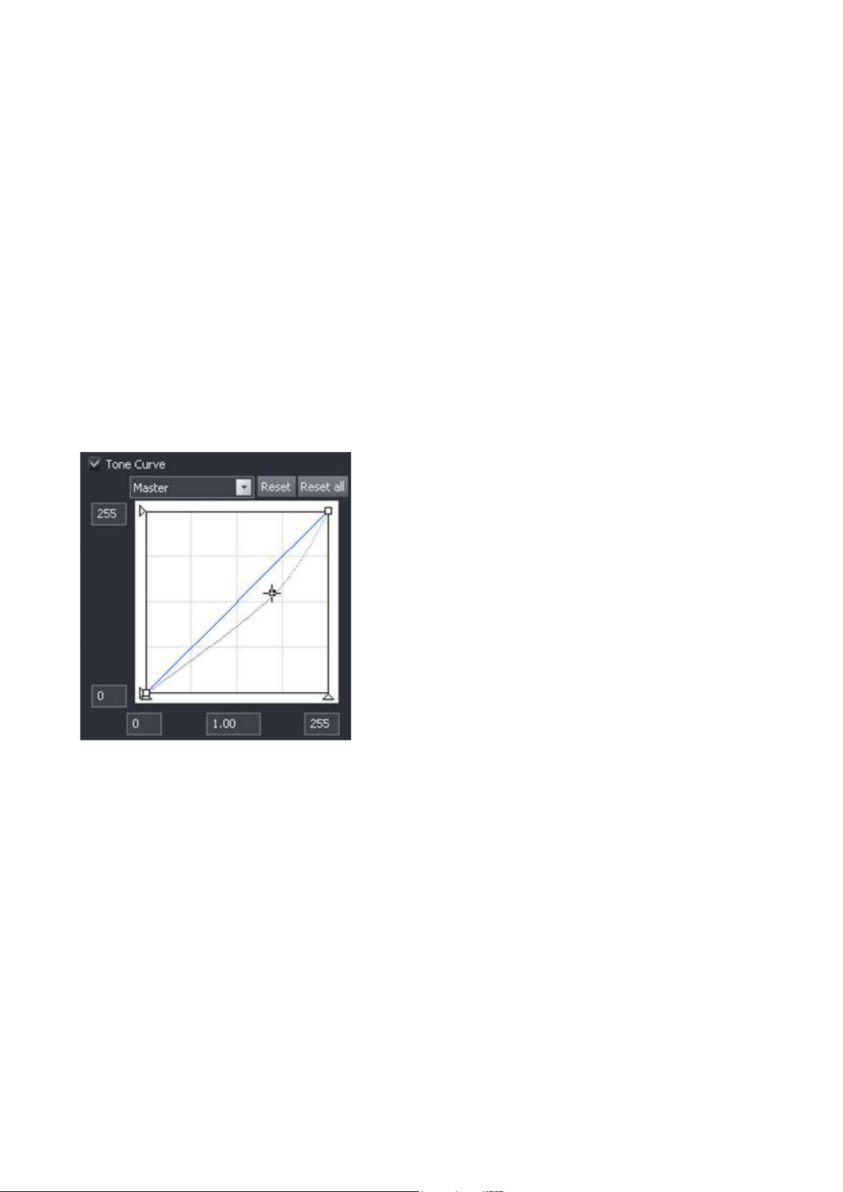
DxO Optics Pro V4.2 Reference Manual

The same goes for the Lightness slider: to the right (or enter a positive figure) to lighten, to the left (or enter a negative figure) to darken. These slider and box values can be from +100 to –100. The action of this slider is slightly interesting, and you’ll probably find it easiest to understand if you look at the result on the Histogram display. Effectively, moving the slider to the right or entering a positive figure lifts the black level towards white, compressing the tonal range into the upper half of the scale. Conversely, moving the slider to the left or entering a negative number brings down the white level towards black, compressing the tonal range into the lower half of the scale. And also as usual, the ‘As shot’ button cancels any HSL correction.

Tone curve

Once again, the panel has a check box to enable this correction, and if the check box is unchecked (correction disabled), the panel controls will be grayed out.

The tone curve is a very powerful tool, but is not, at first, all that easy to comprehend. The graphic indicates the relationship between tonal values into the tool (across the x axis) and out of it (up the y axis). The tone curve represents the transfer characteristic—the way in which input tones are mapped onto output tones. The initial straight line indicates that output tonal values are exactly the same as input values over the whole tonal range.

In order to adjust tone mapping for correction or creative purposes, the straight line is manipulated so as to alter this input/output relationship. In traditional photographic terms, this means altering the gamma of the image, and this graphical approach allows a great deal of flexibility.

Note first that the combo box at the top lets you choose to adjust either the Master channel—i.e. all three colors together—or any of the three Red, Green, Blue channels individually. The buttons to the right enable you to reset either

Page 54

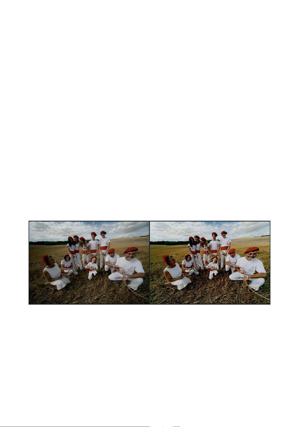
DxO Optics Pro V4.2 Reference Manual

the single curve you are working on, or reset all three of them together, back to the default straight line.

Probably the first step in your manipulation will be to add points to the line, which you do simply by left-clicking on it. As soon as a point is created, you can drag it around, and the line will follow, the curve ‘splining’ as you do so— and you can watch the result live on the preview image. You can create as many points as you need to in order to generate the curve you want. To move a point, simply click on it; the active point is shown filled in black, and inactive ones as hollow white. Likewise, you can delete the active point using the Delete key.

An alternative to drawing a made-to-measure line is to make a numerical entry of the gamma value; the box at bottom center is set by default to a gamma of

1.00, and you can enter any figure between 0.05 and 6.00. As you would expect, a gamma value higher than 1 tends to bring up detail out of the shadows, whilst a value lower than 1 crushes it down into the blacks.

The input and output black and white points can likewise be set, either by dragging-&-dropping the relevant points with your mouse, or entering numerical values in the 4 entry boxes—from 0 (black) to 255 (white).

The Tone curve adjustment is probably the hardest to explain in words, but certainly one of the most useful features in terms of tonal control of your images.

Page 55

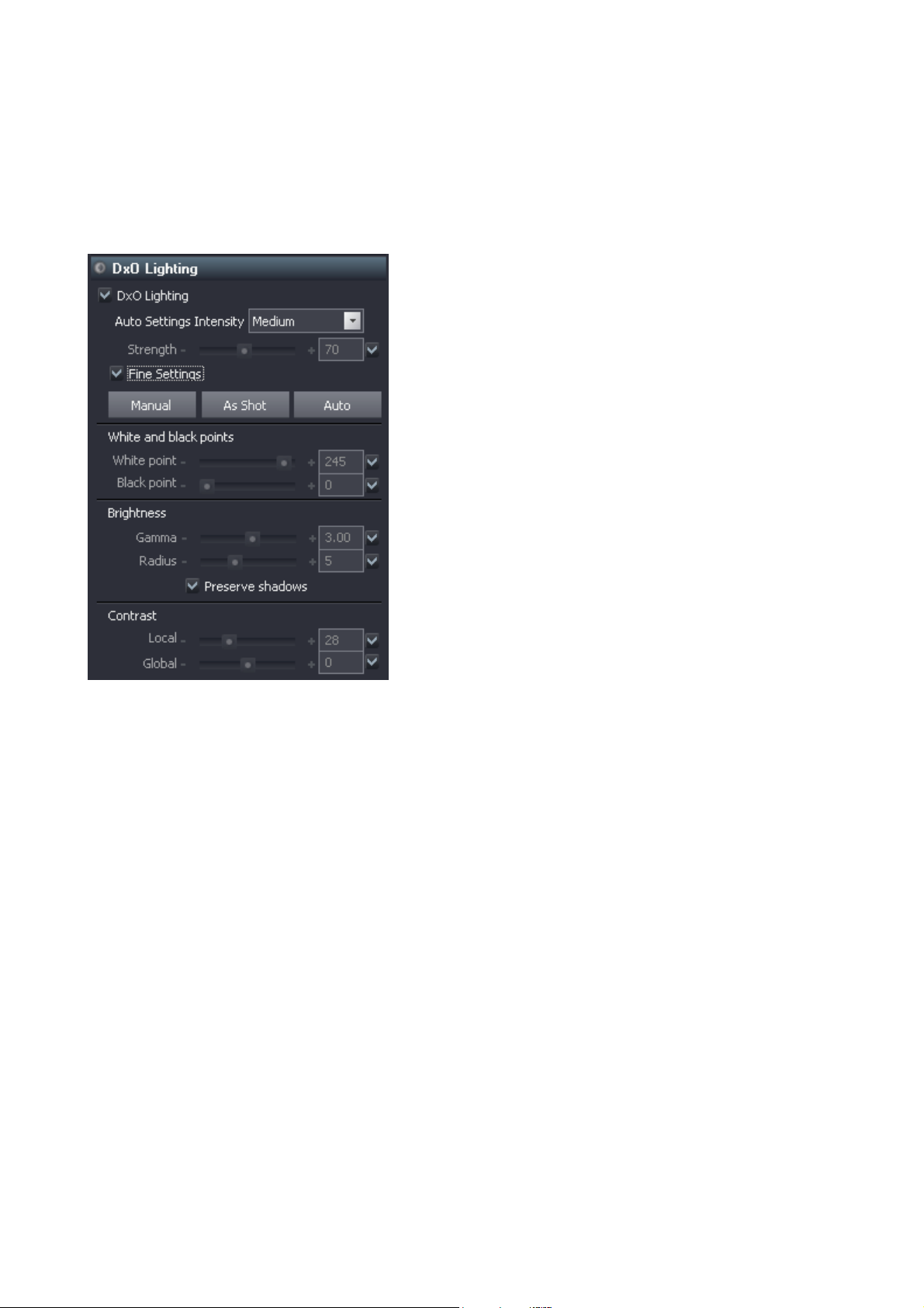
DxO Optics Pro V4.2 Reference Manual

Chapter 16 DxO Lighting tools

This DxO Optics Pro feature merits a little explanation.

Natural scenes rarely exhibit ideal lighting conditions; light sources are often directional and sometimes quite harsh. What’s more, when taking pictures we are often more concerned about capturing the right moment, and pay little attention to potential lighting problems. To compound the problem, the dynamic range of sensors can’t compete with that of our eyes. All this can result in some shots exhibiting under-exposed, dark or shadowed regions with missing details. To a certain extent—basically, when the wanted image signal is sufficiently above the noise level—lighting problems can be corrected afterwards, given appropriate image processing. Pixel-precise image segmentation technology lies at the heart of DxO Lighting, to deliver automatic local contrast adjustment and thereby reveal hidden detail in dark areas. Simply put, DxO Lighting first breaks the image down into a number of areas in which luminance values have a certain range; it then processes each of these areas in the most appropriate manner to reveal detail. In general terms, lightness and tone curve slope are slightly increased in dark areas to bring out detail, yet avoid the signal clipping that could occur if the overall gamma were adjusted.

Page 56

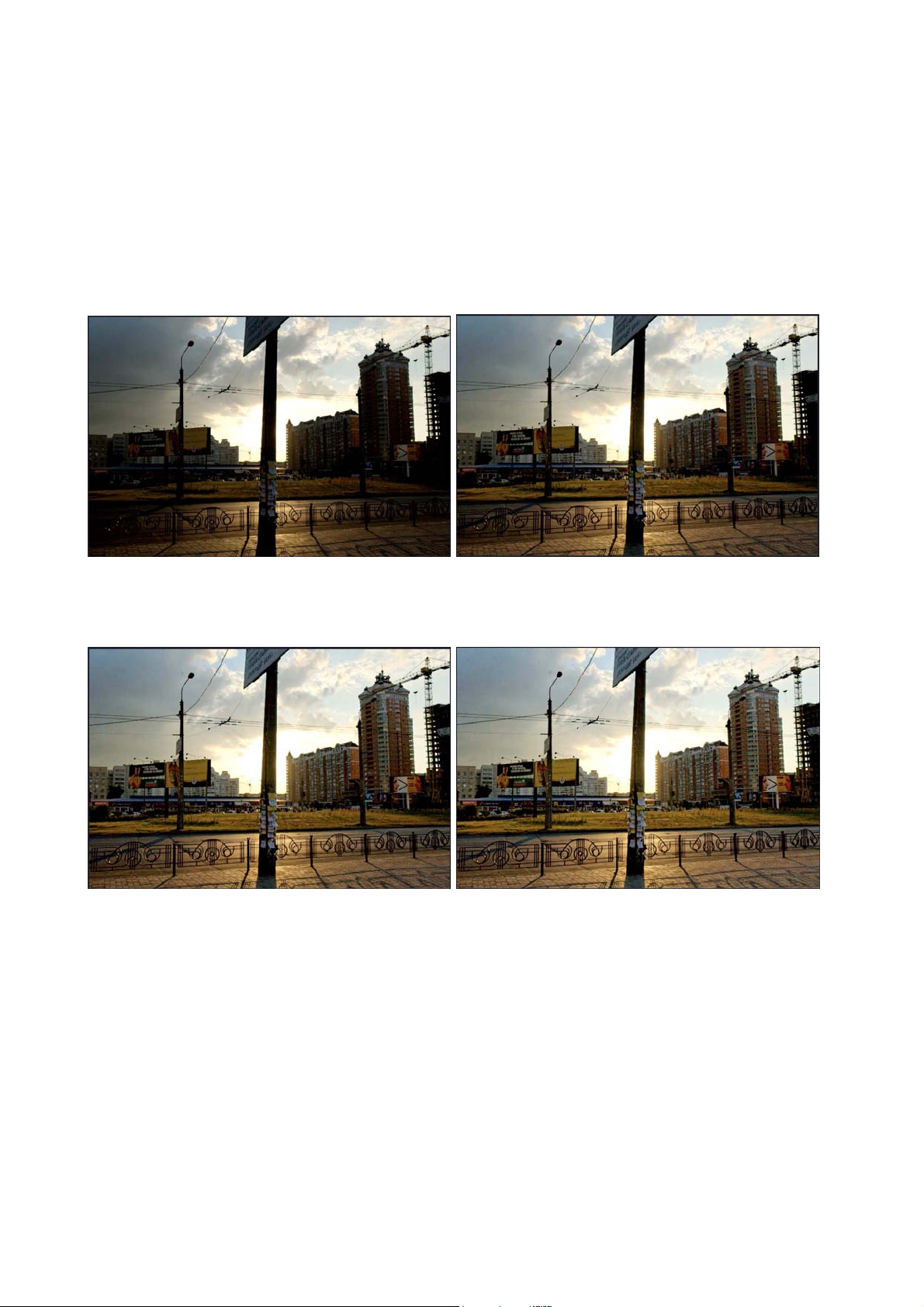
DxO Optics Pro V4.2 Reference Manual

Auto settings intensity Slight / Medium / Strong

There’s a simple check box on the right for Auto, which has to be unchecked to enable the slider for Strength—as usual, the slider is disabled until the Auto box is unchecked. Slider range is from 0 to 150 %, and there’s also an edit box for direct entry of the correction value.

Look at the effect on the four pictures below:

Original image Lighting “slight”

Lighting medium lighting strong

There is the same basic check box for Auto or manual, and the slider for Correction strength—the slider is disabled until the Auto box is unchecked. Slider range is from 0 to 150 %, and there’s also an edit box for direct entry.

Checking the ‘Fine controls’ box opens up a sub-panel with a whole new group of controls. First come the buttons for Manual / As shot / Auto that uncheck / check all of the ‘Auto’ boxes at the same time, and a central ‘As shot’ button that resets all sliders to their default positions—very useful!

Page 57

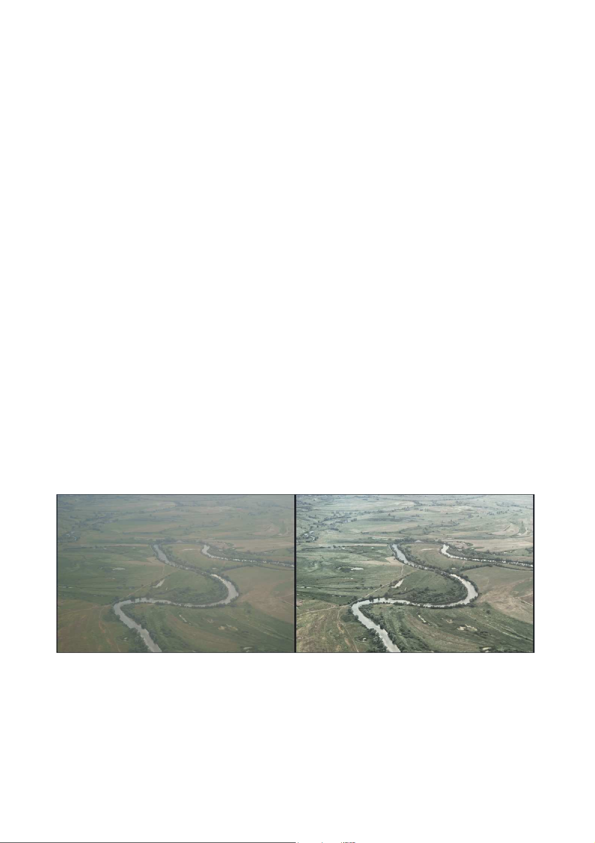
DxO Optics Pro V4.2 Reference Manual

The White and Black point sliders operate in a complementary fashion; each has a range from 0 to 255, or you can enter a whole number in the edit boxes instead. These controls have the effect of stretching the image’s lower tonal range up towards white, or vice-versa: stretching the upper range down towards black. This is similar in many ways to what might be achieved using a tone curve adjustment and is probably easiest to visualize in conjunction with the Histogram display. Selecting or deselecting ‘Auto’ for either automatically selects / deselects it for the other too.

The Brightness adjustment acts basically like an overall gamma control, the slider and entry box having a default setting of 1.00, with a range from 0.50 to

5.00. The Preserve shadow feature (checked by default) operates at higher positive gamma settings, where shadows tend to become washed-out, and intelligently decides to what extent the darker tones should be ‘held back’ as shadows. The Radius slider / edit box affects the way DxO Lighting makes its decisions about what areas represent shadow or not, and how to apply the gamma locally in the image; it has a range from 0 (entirely global) to 15 (fully localized).

And last but by no means least comes the pair of sliders / edit boxes for Local contrast (range from 0 to 100 %) and Global contrast (range from +50 to – 50 %). As you might expect, the Global contrast control uses an S-curve to affect the overall contrast of the image, with a useful bi-directional range allowing both contrast enhancement for slightly flat images and reduction for contrasted ones. The Local contrast control, on the other hand, is more subtle in its effect, altering the contrast in a spatially determined way that takes account of the area around each pixel, having something of the feel of dodging-and-burning.

Page 58

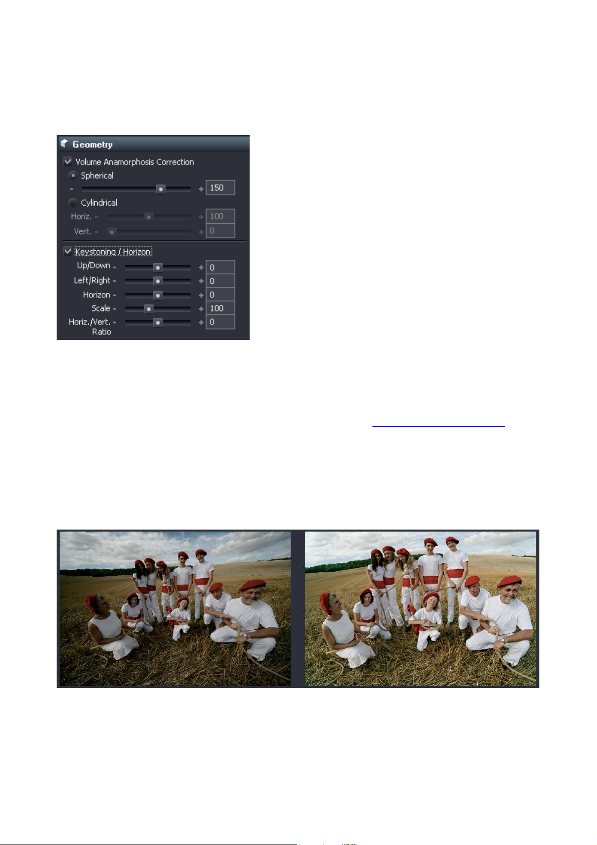
DxO Optics Pro V4.2 Reference Manual

Chapter 17 Geometry tools

Volume anamorphosis correction (VAC)

There is a fundamental problem when capturing a picture of our threedimensional world onto a two-dimensional image, governed by the basic laws of optics. When converted into a flat image, the shapes of certain threedimensional objects seem distorted, so they do not correspond to what our eyes and brain expect to see. This is referred to as ‘volume anamorphosis’, and is most noticeable and objectionable when using wide-angle lenses, and when it affects foreground objects close to the camera. One of the biggest problems when trying to correct for this distortion is that it is entirely picture-content dependent, and because of the trade-offs involved, it is of necessity a subjective, artistic decision that needs to be made by the user.

The distortion is most evident with three-dimensional objects near the camera, and the correction required depends on their underlying shape. Basically, cylindrical objects (for example, columns or full-length human figures) need correction along one axis more than another, which we refer to as cylindrical

Page 59

DxO Optics Pro V4.2 Reference Manual

correction (in a sense that may be either horizontal or vertical), whereas inherently spherical objects (e.g. a human head) need correction on both axes at once; we refer to this as spherical correction and it is actually calculated along a radius from the centre of the picture. Both of these corrections are dependent on the focal length of the taking lens. The VAC panel provides radio buttons for selecting either spherical or cylindrical correction, with a single slider for the former, and a pair of horizontal and vertical correction sliders for the latter. All three sliders and edit boxes can take values from 0–200 %. VAC correction is only possible when geometric distortion (under DxO Optics) is available and applied, so checking the VAC check box will automatically check the geometric distortion box too; conversely, if the appropriate module is not available to enable geometric distortion correction, then VAC will be disabled too.

To adjust these controls, you need first to examine the image and decide what type of correction is required. Choose the appropriate type of correction for the picture content that most needs correcting, and then apply as little correction as possible to render the residual distortion acceptable. Over-correction will start to re-introduce unwanted geometric distortion and you may have to find the best compromise.

Keystoning / Horizon

(a check box enables correction) The pair of Up/Down and Left/Right sliders / edit boxes for adjusting respectively vertical or horizontal keystoning correction both have a range of +100 to –100. The Horizon slider has a range from –180° to +180°, enabling the image to be rotated completely upside down at either extremity of the scale. Equally useful, of course, for correcting leaning verticals. A semi-transparent grid is available, simplifying adjustment of the squareness of the shot (and note that users can choose to set up either a vertical or horizontal line for this, with the tool described below).

Associated with the Keystoning / Horizon corrections is a button

on the top

left of the header bar that accesses a drop down menu with four special tools:

Note that defining your geometric corrections in this way will override any other settings you may have entered via the sliders and/or edit boxes, so you are warned of this and asked if you want to continue. Also note that each of these corrections cancels out the others, so they are effectively mutually exclusive.

Level horizon In the first case, selecting this option lets you define a line in the picture that you want to correct so as to be horizontal (or vertical). To do this, you first

Page 60

DxO Optics Pro V4.2 Reference Manual

stick down one end point with the mouse, then set another end point to define your line, shown by a bright green line on the preview image. As soon as you click the second point, the image will rotate in such a way as to make your chosen line horizontal (or vertical). If you make a mess of it the first time, you can click on Undo [Ctrl + Z] and then reset your second end point. All the remaining three options change the display into twin, side-by-side images, showing the original preview image on the left and the result of your correction on the right. Once the defining points have been set, three new buttons appear at the bottom left: Check, Accept, Reset. In each case, click on the Check button to check the effect in the right-hand preview image, and then either Accept the correction, or click on Reset to go back to the original settings and try again. These three modes also have a check box for ‘Keep image centered’, which can be helpful when shooting architectural pictures, for example.

Force parallel (vertical) Force parallel (horizontal) Force rectangle

The first two keystoning correction options Force vertical / horizontal act in a similar way, except that in these cases you are asked to define a pair of vertical / horizontal lines that you wish to be parallel, and hence, you need to define two pairs of start and end points. It doesn’t matter if you define the lines in the same or reverse sense, the end result doesn’t change. Only the relative angles of the lines count—their lengths have no significance. If you define a pair of horizontal lines for vertical correction (or vice-versa), your image will be rotated to suit.

If your picture contains both vertical and horizontal keystoning at the same time, you will need to use the fourth option, Force rectangle. This lets you define four points that form corners of a quadrilateral that you wish to correct to be rectangular. Note however that this is rather more powerful than a simple manual combination of both vertical and horizontal keystone correction, since it can also introduce an element of ‘skew’ into the correction.

As the four corrections under this button are mutually exclusive, if by any chance your image contains both keystoning and a horizon that isn’t level, you will either have to first perform one of the corrections using the top left-hand buttons and then the other in the Geometry panel of the right-hand palette, or perform all your corrections using the panel controls. Since the Level horizon command only works with a horizontal line, if the problem with your picture is in fact a leaning vertical, it will make most sense to correct any keystoning first using the left-hand button, and only then go and correct the leaning vertical in the right-hand Geometry panel. Alternatively, you can cheat by using the Force rectangle tool, though this gets a bit fiddly!

Page 61

DxO Optics Pro V4.2 Reference Manual

Scale

The Scale slider / edit box lets you resize the image; the default value is of course 100 %, and you can reduce the size to 50 % or increase it to 200 %.

Horiz. / Vert. Ratio

The H / V ratio slider / edit box lets you stretch or squeeze the height of your image while keeping the width unchanged. The scale runs from –100 to +100, which represents from 50 % to 200 % of normal height.

Crop

To crop an image, you can either select the Crop button from the left of the header bar, or open the Crop panel in the right-hand corrections palette, where there is an Enable crop check box. If you have selected Crop from the left-hand buttons, the only way to escape from this is to uncheck the Enable crop button in the panel. Conversely, if you click the top left Crop button, this will automatically check the right-hand panel Enable crop button.

Once Crop has been enabled, a rectangle appears with handles in the middle of each side and at each corner. By dragging these handles, you can move the borders of the rectangle around to adjust the cropping of your image.

On the right-hand panel, there is a drop-down list from which you can choose the way the aspect ratio of the image is controlled in Crop. Unconstrained gives you completely free rein to reshape the crop in any way you like, otherwise a series of fixed ratios will constrain it to always maintain certain proportions, from 1:2 to 1:1, or maintaining the original, ‘as shot’ aspect ratio. A final option allows you to define a Custom ratio, handy if you need for example to crop a whole series of images to conform to a specific aspect ratio. Clicking on Custom opens a small window that invites you to enter numeric values for the ratio you want. These must be integers, but will accept a sufficiently wide range of values to enable any desired proportion to be achieved.

Page 62

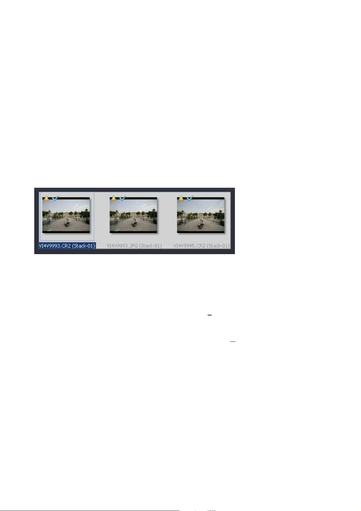
DxO Optics Pro V4.2 Reference Manual

Chapter 18 Stacking, ranking and Output formats

Stacking

A ‘stack’ of images is a way of organizing your images into groups, which can not only help to save clutter on your workspace but, more importantly, enable you to apply various settings to a whole group of images together (without having to multi-select them each time). Any time you have a number of images that for some reason might require the same processing, you may want to consider stacking them. These might be a series of related images of the same subject, or a set of images taken under the same lighting conditions… the possibilities are endless. If one of these images subsequently needs individual settings, you must first unstack it in order to be able to adjust the settings for this particular image.

It is easy to create a stack, either by physically dragging-and-dropping thumbnail images (or filenames) on top of one another in the project pane of your workspace, or by selecting multiple images and then clicking the button of the last-selected image’s thumbnail, or then again by first selecting multiple images and then choosing the ‘Create s

tack’ command from the Images menu. Once a stack has been created, it ‘sticks together’ and can be handled and manipulated as if it were single image, until such time as you click on the thumbnail button to un-stack it, or select the ‘Unstack images’ command from the Images menu. The thumbnail for a stack of images appears with a light-gray border. You can expand the stack by double-clicking on the image, so you can check all pictures inside without unstacking them. To shrink the stack, double-click on the ‘top of stack’ (master) image: it’s the one outlined in blue. You can also change the master image—if the stack is expanded, by double-clicking on another image; or if it’s shrunk, by using the scroll wheel on your mouse. Finally, an image can be stacked/unstacked with the help of the menu that appears with a right-click of the mouse (or Option-Click on Mac).

Page 63

DxO Optics Pro V4.2 Reference Manual

Ranking

To help you organize your workflow most efficiently, there is a system of image ranking that uses stars to indicate the priority of images for processing. The reason for opting to rank images in this way is because processing times for large numbers of high-resolution images can become significant, and so it may sometimes be useful to process certain images before others, so that you can for example take decisions about lower-ranked images on the basis of viewing the final results from higher-ranked ones. Of course there is no absolute qualitative meaning to this ranking system, it is merely a convenient way of indicating some form of priority classification.

Above each thumbnail image, only visible on mouse-over, are a line of stars

 (grayed out at start-up) to indicate the selected ranking of this

image—you can click these stars on or off at any time and in any workspace. In the ‘Organize’ and ‘Enhance’ workspaces, these stars are also permanently accessible in the preview pane.

If you click on the third star  , the ones to the left of it will light up too, like this: 

Later, when you get to the processing stage, you can implement the ‘star ranking’ you set earlier; this is where you select which rank of images to process. There is a button for ‘All’, or again you can click to activate 1, 2, 3, 4, or 5 (individually, or in combination).

You can select a higher-ranking star alone to specifically exclude lower rankings; so

  will process only those images ranked . You can

also make multiple selections, just by clicking on the corresponding stars; so for example   , will process only images ranked either or .

To process all images ranked up to , you need to select . Minithumbnails of the selected images will appear in the column below. Alongside the star buttons is another [ ?] button, which allows you to select only unranked images for processing.

Page 64

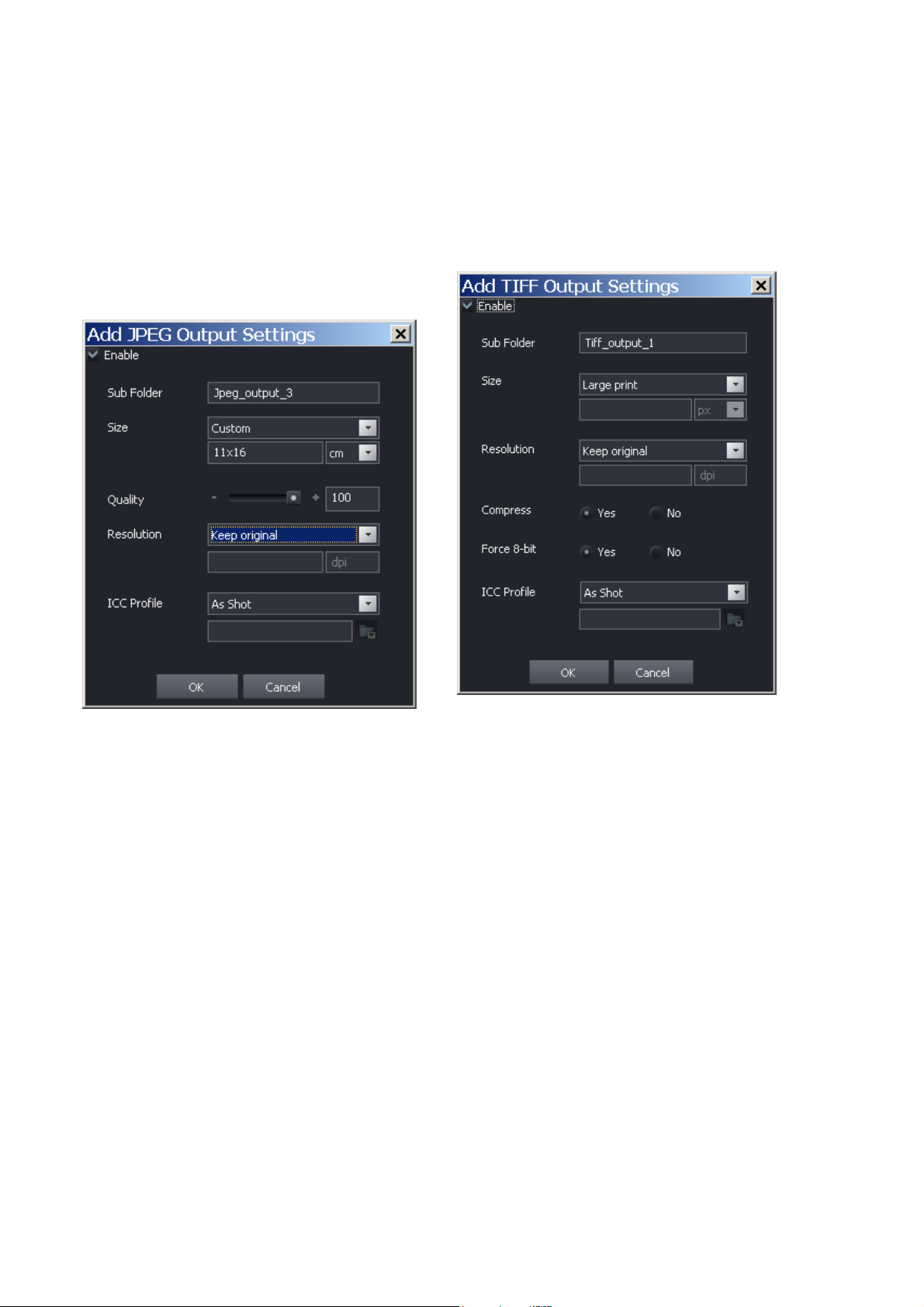
DxO Optics Pro V4.2 Reference Manual

Output Format tab

One of DxO Optics Pro’s great time-saving features is the ability to save images in more than one format at a time. So, for example, you might want to archive processed images in a high-quality format like DNG (only available when originating from Raw images), while at the same time saving a JPEG copy for web-based publication (including destructive compression). What’s more, this new feature in version 4 enables you to create multiple output format settings within each format—so, for example, you might have one JPEG format configured for images destined for website use, and another for making prints.

All of these configurations will be listed under the respective output formats, and you can check the box to enable one or more configurations in one or more output formats—so in a single processing batch you can produce multiple versions of the same image with different output format settings.

The three buttons ‘Add JPEG’, ‘Add TIFF’ and ‘Add DNG’ each open a window where you can select some basic, and some format-specific options.

Page 65

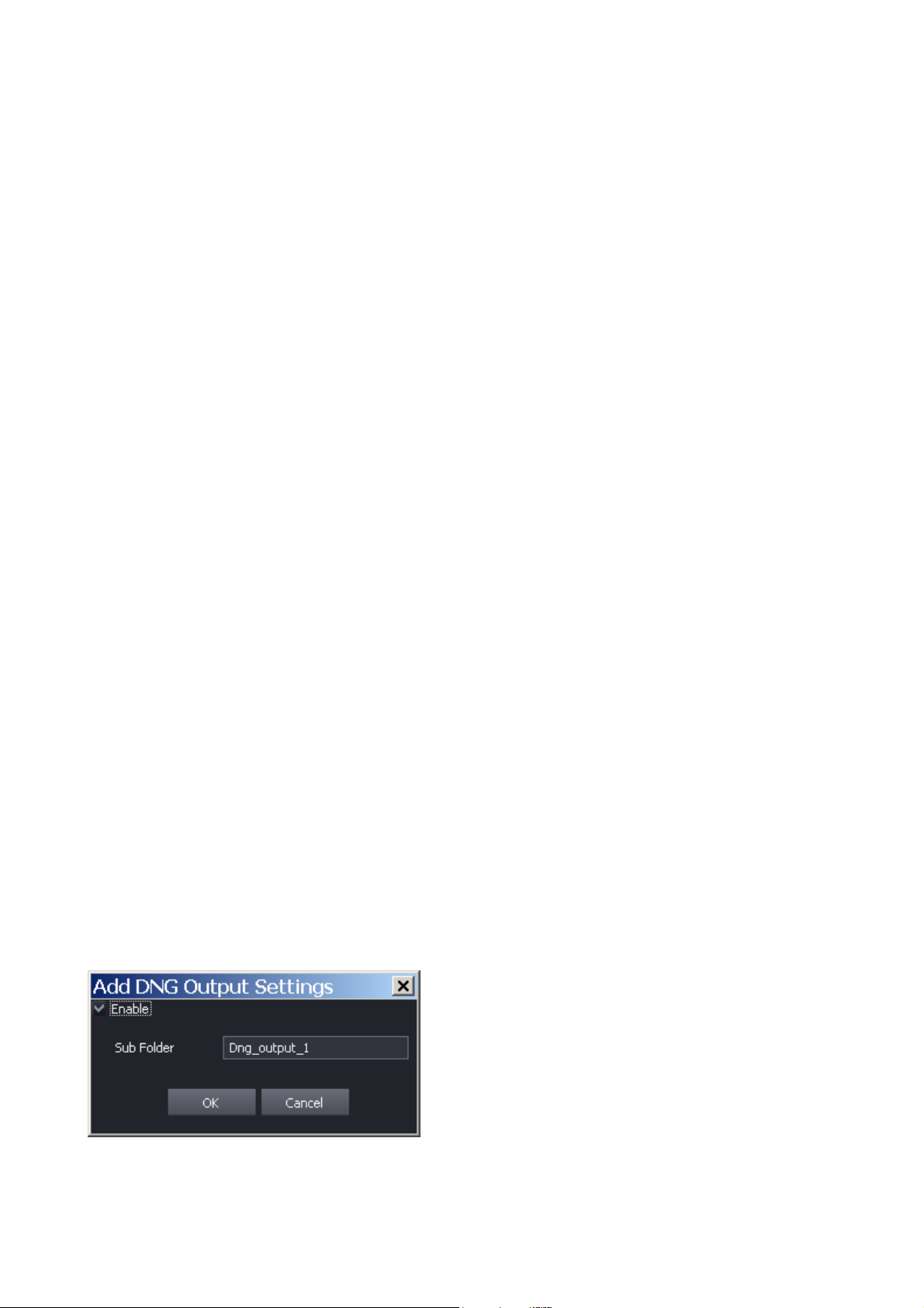
DxO Optics Pro V4.2 Reference Manual

All three windows carry an ‘Enable’ check box at the top left, so you can enable or disable any given output formats for any given images. This check box is duplicated alongside each output format in the list, and at least one output format must be enabled in order for an image to be processed. If you attempt to start processing with no output formats enabled, you will be warned by an error message.

Then a drop-down list lets you choose the intended size and use of your image, which will preset certain parameters like size and resolution. If you select the ‘Custom’ option, the next combo box is activated, which lets you specify an image size in either pixels [px], centimeters or inches. Correct syntax is [dimension]x[dimension], and it doesn’t matter whether you specify image height or width first.

Next, the JPEG window (only) has a slider and edit box for ‘Quality’ that lets you select the degree of JPEG destructive compression, and hence file size, you wish to use. Obviously, you should use as high a setting as you can for maximum quality, unless file size considerations take precedence.

Below this is another drop-down list that lets you choose the resolution you want for your output images, and once again, selecting ‘Custom’ activates the next combo box, which lets you specify an image resolution in dpi (dots per inch).

Finally (on the JPEG window) there is another drop-down list for selecting the output color space (ICC)—this function is for advanced users only, most of the time it can be left on the default setting of ‘As Shot’. If you select ‘Custom’, the browse button [ ] below is enabled and you can go off to locate any custom ICC color profile that you may have created.

The TIFF window is similar to the JPEG one, except that there is no ‘Quality’ setting; instead, there are yes / No radio buttons for ‘Compress’ and ‘Force 8bit’—these are set to ‘Yes’ by default, and again, are settings that should only be changed by advanced users who wish to disable compression and/or use 16-bit encoding.

The DNG window is simpler, having only the text box for setting the subdirectory where output format configuration files will be saved.

Page 66

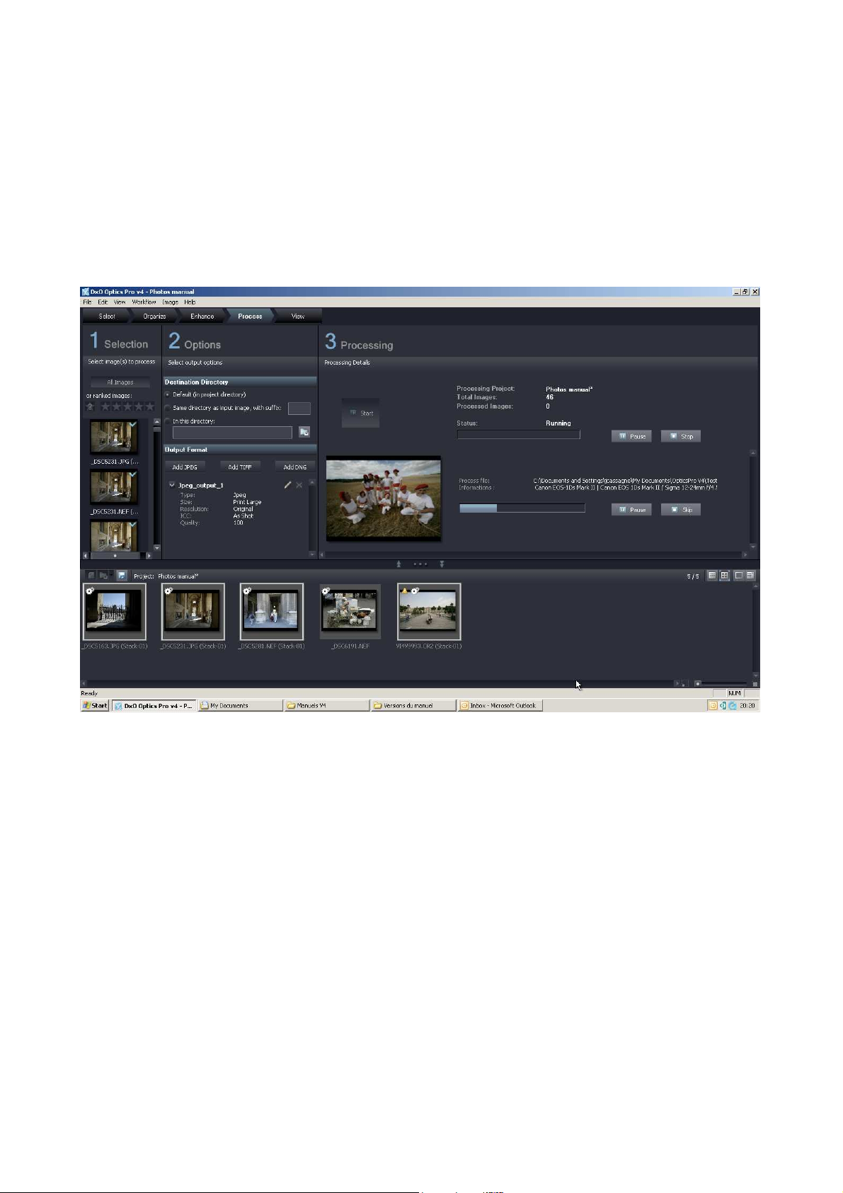
DxO Optics Pro V4.2 Reference Manual

Each output format in the list also has a [pencil] button so you can modify the settings, and a [X] so you can delete it altogether. It is perhaps important to emphasize once again that once you have created a number of output format settings, you can apply one or more of them to any selected image(s). This will only marginally increase processing time, but can obviously lead to the generation of multiple output image files, which may

have an impact on disk space.

Page 67

DxO Optics Pro V4.2 Reference Manual

Chapter 19

DxO Optics Pro plug-in for Photoshop

DxO Plug-In for Adobe Photoshop™

Installation

DxO Optics Pro external module for Photoshop is installed with the help of the DxO Download Manager; you can install it directly at the same time as the application or afterwards (for example after having installed Photoshop on your computer). The Download Manager automatically places a folder called DxO (with the “Import.8ba” file inside), in the “Plug-ins” directory of Photoshop. It is possible that the installer may not place the plug-in in the correct folder, if you have several versions of Photoshop™ (the full version as well as Photoshop Elements for example). In this case, you can move manually the DxO folder in the “Plug-ins” directory of Photoshop™.

Activation and Use

To activate the plug-in, launch Photoshop™ and scroll down the File menu: Under the command “Import”, choose DxO Optics Pro. The usual window of DxO Optics Pro will appear, with one important difference: only the three tabs “Select”, “Enhance” and “Process” are available. Under “Select”, place, as usual, images in the beginning of a Project (that it is not possible to save). Note: in the DxO Optics Pro plug-in for Photoshop, a project can only contain 5 images.

Treat as usual the necessary enhancements, then define in the tab “Process” the output formats that you need. With one click on the Start button, you’ll launch the image treatment. Once treated, the images open in the Photoshop™ window (one window for each image.)