

Page 1

Predictive Analysis User’s Guide
Predictive Analysis 6.5.1
Page 2

2 Predictive Analysis User’s Guide
Copyright
Trademarks
Use restrictions
Patents
Copyright © 2004 Business Objects. All rights reserved.
Business Objects, the Business Objects logo, Crystal Reports, and Crystal Enterprise are
trademarks or registered trademarks of Business Objects S.A. or its affiliated companies in the
United States and other countries. All other names mentioned herein may be trademarks of their
respective owners.
This software and documentation is commercial computer software under Federal Acquisition
regulations, and is provided only under the Restricted Rights of the Federal Acquisition
Regulations applicable to commercial computer software provided at private expense. The use,
duplication, or disclosure by the U.S. Government is subject to restrictions set forth in
subdivision (c)(1)(ii) of the Rights in Technical Data and Computer Software clause at 252.227-
7013.
Business Objects owns the following U.S. patents, which may cover products that are offered
and sold by Business Objects: 5,555,403, 6,247,008 B1, 6,578,027 B2, 6,490,593, and
6,289,352.
Page 3

Predictive Analysis User’s Guide 3
Contents
Preface Maximizing Your Information Resources 5
It’s in the documentation . . . . . . . . . . . . . . . . . . . . . . . . . . . . . . . . . . . . . . . . 6
Chapter 1 Introduction to Predictive Analysis 9
Important concepts . . . . . . . . . . . . . . . . . . . . . . . . . . . . . . . . . . . . . . . . . . . . 11
Chapter 2 Configuring Predictive Analytics 13
Population . . . . . . . . . . . . . . . . . . . . . . . . . . . . . . . . . . . . . . . . . . . . . . . . . . 15
Derived variables . . . . . . . . . . . . . . . . . . . . . . . . . . . . . . . . . . . . . . . . . . . . . 19
Create new binning . . . . . . . . . . . . . . . . . . . . . . . . . . . . . . . . . . . . . . . . . . . 23
Models . . . . . . . . . . . . . . . . . . . . . . . . . . . . . . . . . . . . . . . . . . . . . . . . . . . . . 29
Chapter 3 Influencer Analytics 39
Influencer analytics . . . . . . . . . . . . . . . . . . . . . . . . . . . . . . . . . . . . . . . . . . . 41
Goal based influencer detail . . . . . . . . . . . . . . . . . . . . . . . . . . . . . . . . . . . . . 44
Influencer gains chart . . . . . . . . . . . . . . . . . . . . . . . . . . . . . . . . . . . . . . . . . . 46
Models gains chart . . . . . . . . . . . . . . . . . . . . . . . . . . . . . . . . . . . . . . . . . . . . 48
Variable profile box plot . . . . . . . . . . . . . . . . . . . . . . . . . . . . . . . . . . . . . . . . 51
Influencer detail . . . . . . . . . . . . . . . . . . . . . . . . . . . . . . . . . . . . . . . . . . . . . . 54
Chapter 4 Lists and Forecasts 57
Metric forecaster . . . . . . . . . . . . . . . . . . . . . . . . . . . . . . . . . . . . . . . . . . . . . 59
Individual list . . . . . . . . . . . . . . . . . . . . . . . . . . . . . . . . . . . . . . . . . . . . . . . . . 62
Contents
Page 4

4 Predictive Analysis User’s Guide
Chapter 5 Appendix 65
Forecasting Algorithm . . . . . . . . . . . . . . . . . . . . . . . . . . . . . . . . . . . . . . . . . 66
Universe configuration . . . . . . . . . . . . . . . . . . . . . . . . . . . . . . . . . . . . . . . . . 68
To check the population query . . . . . . . . . . . . . . . . . . . . . . . . . . . . . . . . . . 70
To test derived variables . . . . . . . . . . . . . . . . . . . . . . . . . . . . . . . . . . . . . . . 71
Model building . . . . . . . . . . . . . . . . . . . . . . . . . . . . . . . . . . . . . . . . . . . . . . . 72
Appendix A Glossary of Terms 73
Index 77
Contents
Page 5

Maximizing Your Information Resources
preface
Page 6

6 Predictive Analysis User’s Guide
It’s in the documentation
Predictive Analysis documentation strives to deliver product information that is
rich, convenient, and easy-to-use.
Whether you’re a novice or experienced user, Predictive Analysis documentation
is the place to go for discovering our product, e xploring their features, or locating
precise information.
Product information has been substantially expanded to encompass not only
facts about product features but also tips, samples, and troubleshooting
instructions.
For your convenience, our documentation is available from all products in
Acrobat PDF, and print media.
Documentation has been designed first and foremost with speed and ease of
navigation in mind. All the information you require is readily available just a few
mouse clicks away.
The next sections highlight new and key features of our documentation.
Online guides
!
User’s guides
All Application Foundation user’s guides are available as Acrobat Portable
Document Format (PDF) files. Designed for online reading, PDF files enable you
to view, navigate through, or print any of their contents.
From a PDF file, you can search for specific occurrences of a word using the Find
command, or navigate to the exact location of a topic by clicking a crossreference or an entry in the Index or Table of Contents.
To open a document, you can select it from the Help menu provided that you
have installed the Adobe Reader, version 5.0 or higher on your machine. You can
download it for free from Adobe Corporation’s web site at:
http://www.adobe.com/products/acrobat/readstep.html
What to do fo r m o re in formation
If you cannot find the information you are looking for, then we encourage you to
let us know as soon as you can. Feel free to send us any requests, tips,
suggestions, or comments you may have regarding this or other Application
Foundation documentation using the Reader’s Comment Form at the end of this
chapter.
Maximizing Your Information Resources
Page 7

Audience
Predictive Analysis User’s Guide 7
To search for anything specific use the index.
Below is a list of other Application Foundation guides:
• Dashboard Manager User Guide
• Set Analysis User Guide
• Process Analysis User Guide
• Application Foundation Installation Guide
• Application Foundation Configuration Guide
This guide is intended for anyone interested in performing simple to complex
customer-related segment analysis from any Java-enabled Web browser that is
connected to the Internet or a corporate intranet.
For information regarding the installation and configuration of Application
Foundation, see the Application Foundation Installation Guide and Application
Foundation Configuration Guide.
It’s in the documentation
Page 8

8 Predictive Analysis User’s Guide
Reader’s comments form
Predictive Analysis User’s Guide
Version 6.5.1
Part Number: 3C1-50-300-01
Your company’s name: _______________________________________
Company address: __________________________________________
Telephone/fax number: _____________ E-mail address: ____________
What is your job position? _____________________________________
How long have you been using Predictive Analytics? ________________
Business Objects welcomes your comments and suggestions on the qual ity and
usefulness of this publication. Your input is an important part of the information
used for revision.
If you find any errors or have any suggestions, please indi cate the topic, chapter
and page number below. Use additional pages if need be.
_______________________________________________________________
_______________________________________________________________
_______________________________________________________________
_______________________________________________________________
_______________________________________________________________
_______________________________________________________________
E-mail your comments to:documentationusa@businessobjects.com
Mail it to:
Technical Publications
Business Objects Americas
3030 Orchard Parkway,
San Jose, CA 95134
Maximizing Your Information Resources
Page 9

Introduction to Predictive Analysis
1
chapter
Page 10

10 Predictive Analysis User’s Guide
Overview
Predictive Analysis and Predictive Analytic Services enable users to discover
data relationships and expose them in different ways. For example some of the
new analytics quantify and communicate relationships between descriptive
variables-such as age, income, and purchasing behavior, on the one hand, and
business outcomes like profitability or campaign response, on the other. Lining
up these relationships side by side can help users optimize business outcomes
by showing them how different factors drive different elements of their business.
Predictive Analysis also introduces box plots and a new form of metric
forecasting that automatically takes cyclical patterns into account.
Introduction to Predictive Analysis
Page 11

Important concepts
There are some basic concepts to understand in data mining. They are:
Population
A Population is a named query that defines a group of interest, using BO
conditions as well as AF sets.
Variable
A "variable" is simply a measured characteristic or attribute. Conceptually, it is
like a database field or a column in a spreadsheet. It may be "actual data" or data
that is derived by means of a look-up, aggregation or other calculation. In
Application Foundation, a variable can be:
• A dimension defined in a BusinessObjects Universe,
• A measure or
• A "Derived Variable," representing a calculation based on measures,
dimensions and/or sets that is defined interactively by a user in Predictive
Analytic Services.
Binning
A binning is a way of compressing the range of values of a variable into a smaller
number, for example, binning of age into age groupings. Binnings may be
explicitly defined or statistically derived.
Predictive Analysis User’s Guide 11
Model
A model is a user-specified configuration of the predictiv e calculati on engine. To
set up a model, the user selects influencers, goals, and the population within
which relationships is quantified.
Goal
A goal is a variable which can be numeric or boolean variable used as a (positive
or negative) outcome of interest. It can represent purchase volume, account
closure, equipment downtime, or supplier backlog.
Goal-based binning
A special kind of binning is one that is optimized for a goal or outcome. The
purpose of such a binning is to emphasize only those distinctions in the value
range for an Influencer that correspond to significant shifts in the rate or mean
value of a specified goal variable. For example, it may be that the only impo rtant
Important concepts
Page 12

12 Predictive Analysis User’s Guide
distinctions in age of prospect that affect response rates to a marketing campaign
are "under 20, 20-63, and 64+." The Influencer modeling engine automatically
calculates these during model generation.
Influencer
An influencer is a variable used as a descriptive or behavioral piece of
information, such as age, state of residence, or calculations such as "months
since first purchase."
!
Influencer data types: nominal, ordinal and continuous
All variables have a data type. In BusinessObjects, the primary data types are
character, numeric, and date. For Influencer Analysis, however, a slightly
different (statistically-motivated) classification is used.
• Nominal
Nominal variables are those whose values are not inherently ordered.
Examples are Gender and Marital Status. All character objects from a
BusinessObjects universe are treated as nominal. In addition, Derived
Variables whose data type is Boolean (for example, whose only values are 0
and 1 are treated as Nominal.
• Continuous
Continuous is the default data type corresponding to numeric variables. It
should not be used, however, for variables that represent numeric codes
rather than actual numbers (for example, zip code); such variables should be
treated as nominal.
• Ordinal
Ordinal variables are those that have an ordering, but lack proportionality, for
example, the distance between adjacent values is undefined (for example, a
variable whose values correspond to very high, high, medium, low, and very
low). In Predictive Analytical Service, Ordinal is recommended for numeric
variables, whenever.
Introduction to Predictive Analysis
Page 13

Configuring Predictive Analytics
2
chapter
Page 14

14 Predictive Analysis User’s Guide
Overview
This chapter details how to configure for predictive analytics. It also details how
to create and use binnings. Binning is a way of compressing all values for a
variable into a smaller number by subdividing the range of possible values into
groupings or "bins".
The main purpose of Predictive Analysis in Appl ication Foundation is to help you
quantify relationships and anticipate the future. To use any Predictive Analytic,
you have to make sure that the models are defined which are used to perform the
calculations. Models are created to make prediction based on existing
information; perform statistical calculations and find optimal binning of an
influencer with respect to a goal.
Through the configuration section you work towards defining a model and what
needs to be defined before finally using a model to configure analytics and
model-based metrics.
NOTE
Refer to Appendix for trouble shoot.
Configuring Predictive Analytics
Page 15

Population
Population is a named query that defines a group of interest. The next few s teps
allow you to understand the process of creating a new population or editing/
removing an existing one.
NOTE
For more information on population query refer to the appendix.
As you click the population sub-tab, a list of existing populations for the selected
subject area can be seen. Based on the selected name, the details are displayed
on the right side of the list. Population can be either set or enterprise based. You
can view the list by Sets, if the subject area is set-based
Predictive Analysis User’s Guide 15
Population
Page 16

16 Predictive Analysis User’s Guide
!
Create a new population
To create a new population follow the steps below:
1. Click Add icon.
The Create Population window appears. For a new population you have to
define the set it belongs to, (set-based subject areas only) the filters used and
the basic attributes.
2. Select the Set from which you wish to create a population.
Click the drop- down list and make a selection.
3. Once you have selected the set, you need to select the sub set condition.
Depending on the subset condition, you may have to select a second set (for
example, source and destination sets for the "migrant" subset type).
When you create a new population you can chose to pick a population either
from a time period or for a particular month. If you define a time period you
can select From - Through dates.
You can switch between For and From to select two different subsets.
4. Check any one of the option buttons to either pick from the last few periods or
for a particular month.
If you click for a month, you can click the calendar to pick the month. Or you
can use the drop-down list to pick the month and the year.
Configuring Predictive Analytics
Page 17

Predictive Analysis User’s Guide 17
5. Click Next to move to the second section of defining the population.
Here you can apply additional filters that have been defined for the subject
area in a BusinessObjects universe. (This step is optional for set-based
subject areas.)
6. Select the filter name and click the arrow button (or double click the filter
name) that moves the selected filter to the active area.
Optionally, repeat the process to add additional filters.
7. Click Next to define the attributes for the population.
8. Enter the Name of the population being created.
Population
Page 18

18 Predictive Analysis User’s Guide
9. You can make this population public which al lows everyone to view it or keep
it private (you can also start with it being private and change it to public later).
To make it public check the radio box. By default it is private.
10.Click Finish to complete and create a new population.
In case you wish to make any changes, you can click Previous and move back
to previous windows.
As you click finish, the new population listed with all its defined details is
displayed.
You have now defined the population which you can use to create a model.
Configuring Predictive Analytics
Page 19

Derived variables
Derived Variables are user-defined data elements that are derived from
BusinessObjects universe objects and/or set membership. The BusinessObjects
universe itself already supports variable definition in the form of measures and
dimensions calculated from source data. However, users or application
architects may wish to expand the range of variables available for Predictive
Analysis in a safer and more convenient way than by changing or adding
universes to the installation. In addition, some of the Predictive Analysis require
Boolean goal variables, which can only be enabled through the use of Derived
Variables.
These are:
• Model Gains Chart and
• Influencer Gains Chart
Other uses for derived variables include:
• Specifying different date restrictions on measures that calculated
aggregations from fact tables
• Creating duplicates of universe measures for cross-sell analysis
• Creating a variable that represents membership in a specified set (for
example, member of "Frequent Buyers")
• Experimenting with private variables representing alternative approaches
before choosing one to make publicly available
Derived variables are currently exposed for use in:
• Model definition
• Binning
• Advanced Metrics
• Predictive Analysis
• Individual List analytic
Predictive Analysis User’s Guide 19
NOTE
To test derived variable, refer to appendix for details.
Use of derived variable for fact table aggregates
AF3.0 Predictive Analytic Services enable users to define Derived Variables,
using a formula editor. Key usage of Derived variables is to enable users to use
fact table data in predictive analysis.
Derived variables
Page 20

20 Predictive Analysis User’s Guide
Derived Variable Syntax for Measures
The general syntax for measures used in derived variable definition is as follows
(square brackets [] represent optional parameters):
<m:Measure name,
Null value replacement constant,
[<t:Aggregate type>, [Date expression], [Date expression]]
>
Measures are numeric values and can be combined with arithmetic or logical
operators to form more complex expressions.
EXAMPLE
<m:Profit, 0,<t:Sum>, {1/1/2002}, CurrentDate()>
Sum of profit from 1/1/2002 until today, with nulls replaced by 0
<m:Order Size, 100,<t:Maximum>, CurrentDate() - 30*6, CurrentDate()>
Maximum order size in the last 180 days, with nulls replaced by 100
<m:Order Size, 0, <t:Maximum>,
Date(CurrentYear(), CurrentMonth()-6, CurrentDay()), CurrentDate()>
Maximum order size in the last 6 months with nulls replaced by 0
Create a new variable
To create a new derived variable follow the steps below:
1. Select the subject area under which you wish to create a new variable.
Click the drop-down list and select the subject area name.
2. Click Add.
A drop-down appears from which selects the New derived variables.
The Variable Definition window pops up.
3. Enter the new Variable Name.
4. Define whether you want this variable to be public and viewed by all or not.
If not then do not check the box. By default the variable is set to private.
Configuring Predictive Analytics
Page 21

Predictive Analysis User’s Guide 21
5. Select the data type of the variable.
The drop-down lists four types - Boolean, Date, Numeric and Character.
- Boolean is a special type that represents a logical condition whose values
can only be the logical values of TRUE or FALSE. Internally, these are
represented as 1 and 0, respectively. Boolean variables are required to be
used for goals when a binary goal is desired. Currently only Boolean variables
as goals can be profiled in Model Gains and Influencer Gains analytics.
Logical operators and the isinpopulation() function are especially useful for
defining Boolean variables.
- Formulas resolving to a date can be treated as either a data or a numeric
value, representing a monotonically increasing number of days. When used
in model definition, it is usually best to avoid explicit dates such as "date of
birth" and rely instead on numbers representing differences between dates,
such as "age" defined, for example, as "currentDate() - DateOfBirth."
6. You now need to specify how the variable's values are derived.
To do this, you must define a formula in the formula window, using a valid
syntax. There are four types of source data you can make use of.
They are:
- Dimensions from the BO universe corresponding to the selected subject
area
- Measures from the BO universe
- Membership in a set associated with the selected subject area (if the subject
area is set-based)
- Date functions that return the current date, current month, etc. bas ed on the
app server clock.
These can be combined or transformed using operators, functions and
aggregations to arrive at a derived variable definition.
7. To use a Dimension, select "Objects" in the left drop-down (this is the default
selection), and double-click an item that has the blue "Dimension" icon next
to it.
This causes its name to appear in the formula window, encased in angle
brackets and prefixed by "d:" to indicate that it is a dimension.
8. To use a Measure, select "Objects" and double-click an item that has the pink
circle "Measure" icon next to it.
There are two types of measures from the standpoint of derived variable
definition: those with prompts and those without. Measures without prompts
are used "as is." An example is a measure representing a numeric field of a
dimension table, like "age."
The other kind of measure is a time-based aggregate, such as "sum of
Derived variables
Page 22

22 Predictive Analysis User’s Guide
revenue in the past 30 days" or "time (sum of days) since l ast order." In these
cases, additional information is required to resolve the value namely.
- Null value substitution constant
- Aggregation type
- Starting date
- Ending date
9. To select an aggregation type, choose Aggregation from the left drop-down
list and double click the desired aggregation type.
10.To select a date, either click Calendar to choose an explicit date, or else click
the + next to "Date Functions" in the right-hand side selection list and double
click the desired date function.
NOTE
The value of these functions is resolved at the time they are used by an analytic or
analytic service to determine the value of the derived variable.
11.After inserting a Measure that represents a time-based aggregate into the
formula area by double-clicking the name, you must enter appropriate values
for the parameters in the above order just before the closing angle bracket
(">") for the measure definition in the formula area.
Here are two examples of what the end result can look like:
max of profit from 180 days ago until today with nulls replaced by 0 <m:Profit,0, <t:Maximum>, CurrentDate() - 30*6, CurrentDate()>
max of profit from 6 months ago until today with nulls replaced by 10 <m:Profit,10, <t:Maximum>, Date(CurrentYear(), CurrentMonth()-6, CurrentDay( )),
CurrentDate()>
max of profit from 180 days ago until today, with nulls (for example, no purchases)
replaced by 0 -
<m:Profit,0, <t:Maximum>, CurrentDate() - 30*6>, CurrentDate()>, 0 >
.To use membership in a population for derived variable definition, you must use
the isinpopulation() function with the following parameters:
- Population Name
EXAMPLE
1 (True) if customer is a member of the Active Buyer’s set, otherwise 0 (False)
isinpopulation(Active Customers
12.Once you have specified the function enter Save to save the derived variable.
Configuring Predictive Analytics
Page 23

Create new binning
NOTE
If you are familiar with Application Foundation sliced metrics, a binning is similar to
the definition of the entire dimension of slices.
To create a bin first select a variable for example, a dimension, measure or
derived variable.
1. Click New tab an select the New Binning option.
The Binning Initial Parameters Definition window pops-up.
Predictive Analysis User’s Guide 23
The binning is for the selected variable.
Create new binning
Page 24

24 Predictive Analysis User’s Guide
2. Enter a Binning Name.
By default it picks the variable name.
To differentiate the binning you are about to create from other binnings for the
same variable, you can, for example, append the number of bins to the
variable name (for example, "Orders 10").
3. Define whether you want this binning to be public or private.
To make it public, you must check the "Public" checkbox. By default the
binning is set to private.
The variable name is displayed. The Type is dependent on the variable
selected.
4. Enter the Number of Bins you want to start off with.
You can change the number of bins later via Edit.
You can directly enter the number or click the increase/decrease sign.
"Calculation" determines the manner in which the binning engine attempts to
create bins based on the population you specify.
• For numeric variables, the options are "equal count" or "equal width." Equal
Count attempts to arrive at a binning in which the number of records in the
specified working population that fall into each bin is approximately the same
("binning into quartiles"). Equal Width attempts to create bins whose value
range is the same width (for example, a binning of age into 5 year intervals).
• For nominal (character) variables, the options are "equal count" or "equal
categories." Equal count is the same as for numeric variables, except there is
no assumed ordering in which values are grouped together. Equal Categories
tries to arrange for each bin to group together the same number of distinct
values (for example, a binning for State of Residence, where each bin
contains the same number of states). For nominal variables, it may be easiest
to choose a small number of bins, for example, 2, and then create additional
bins via Edit.
5. For numeric variables, you can specify a range of values.
This constrains the bin definitions to the value range you specify.
Configuring Predictive Analytics
Page 25

Predictive Analysis User’s Guide 25
6. Select the population to use to calculate the initial bin definitions.
In Predictive Analysis, new binnings are defined with the aid of a reference
population. This population helps by providing you with some quick feedb ack
on the number of records that fall into specific bins. After a binning has been
defined, the population is no longer retained-only the bin definitions.
If the variable is numeric you do not need to select a population. If y ou select
a numeric variable, the screen shot is slightly different.
7. Click OK to create the new binning under a selected variable.
Edit a binning
The following steps detail how to edit an existing binning.
1. To edit a created binning select the binning category created.
2. Click Edit.
On the window you can see the actual binning that was created based on the
Create new binning
Page 26
26 Predictive Analysis User’s Guide
calculation selected. You can change the binning details through this option.
The first step allows you to change the population to use for profiling the bins.
3. Click the population name.
4. Click Next.
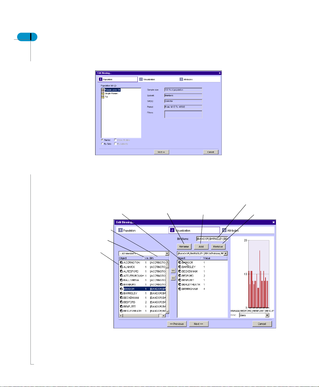
The next window helps your visualize the binning that you have created. If the
binning selected is Nominal variable type, you see the screen below.
Cities assigned to the bin
Rename a bin
Add a new bin
Change bin name
Remove a bin
Bin
Count
listing
City
Configuring Predictive Analytics
Page 27

Predictive Analysis User’s Guide 27
We have taken City as a variable and created a binning for it. At the time of
creating the binning, the calculation was to create equal count for all categories.
What you see here is that all cities have been listed and categorized under bins
and the value for that bin. All members are also grouped into bins. The Value
column represents number of records.
5. Add, Remove or Rename the bin by clicking the appropriate button.
6. On the same window you can also visually see the size of each bin.
You can also see when you add or remove a bin.
7. Click Next to change attributes of the binning.
You can change the name or make it public.
8. Click Finish to complete and save the changes.
Create new binning
Page 28

28 Predictive Analysis User’s Guide
9. If the selected bin type is Continuous, then you see the screen below.
Change working mode
Change bin count
Define bin boundaries
Click bar to select a bin
Refresh Graph
View graph
10.On this window you can do the following:
- Change the working mode of the bin. It can either be by count or by
boundaries.
- If the mode is by boundary:
You can define the minimum and the maximum value for the boundary.
You can view the graph either by regular (fixed) bin width or "actual" bin
width, where the bins vary in width based on their definition.
- If the mode is by count:
You can select a bin by clicking the graph and update the bin definition to
reflect a desired count in the population you are profiling against. The
binning adjusts to approximate the desired bin size.
You can control how the adjustments in bin definitions takes place by
choosing "Selected Bins" mode. (By default, the changes you make to the
target size of the select bin is achieved by modifying adjacent bin
boundaries.)
11.Follow the steps 9 and 10 to complete the process for nominal variable type.
Configuring Predictive Analytics
Page 29

Models
Predictive Analysis User’s Guide 29
Now that you have defined the population and the derived variables it is time to
build a model.
NOTE
To create a model, it is not necessary to define a derived variable.
NOTE
Refer to the appendix for tips to build models.
1. Click New tab which allows you create a new model.
As you click this tab the Model Edition window pops-up. Here you see that you
have to define all the four steps to complete a model.
2. Select the population from the list.
The first section is population. All these populations are defined in the
Models
Page 30

30 Predictive Analysis User’s Guide
population tab.
3. Click Influencers.
You can pick any of the variables from the list. There are dimension,
measures and derived variables. Either click the arrow button or double click
the variable to move it into the active area and treat it as an influencer.
As you move the influencer you notice that the data type is displayed. Also the
associated binning is displayed with the data type. The default binning is
optimal type.
The table illustrated is useful for various data types.
Sources Source Data Type Influence Data Type Goal Data Type
BO Objects Character Nominal N/A
Derived Variable Boolean Nominal Boolean
Configuring Predictive Analytics
Numeric Continuous
Ordinal
Continuous
N/A
Date N/A N/A
Character Nominal N/A
Numeric Continuous
Ordinal
Continuous
N/A
Date N/A N/A
Page 31

Predictive Analysis User’s Guide 31
The next step is to choose one or more goals or outcome variables that you are
interested in understanding or predicting. The model calculates a variety of
statistics based on the influencers and the goals defined. Currently, Predictive
Analysis only supports continuous (numeric) variables (dimensions, measures or
derived variables) and Boolean derived variables as goals.
4. Click the listed variables which can be metrics, dimensions or derived
variables.
Move them to the active side by clicking the arrow or double clicking the
variable name.
You now have to enter the attributes for the model.
5. Enter the Model Name.
6. Define whether you want this model to be public.
Models
Page 32

32 Predictive Analysis User’s Guide
If so then check the box. By default the model is set to private
7. You can specify the Refresh type for a model in two ways.
- With Set: this precipitates a model refresh whenever the set being used in
the associated population definition is refreshed.
- Independent: Model refresh is scheduled independently of set refresh - for
example, through the scheduler or a rule.
The scope of model refresh can be two-fold:
• Refresh Statistics only: this causes the refresh of most statistics and metrics
associated with the model whenever the model is refreshed.
• Regenerate model: this not only refreshes the statistics, but also re-generates
the optimal binnings and recompute the formulas used in generating model
scores (exposed in Individual List analytic). A few statistics are also calculated
only at the time of model regeneration - Net Relevance, in particular.
NOTE
Regenerating a model requi res much more computati on time than does statistics only
refresh, as it necessitates multiple passes through the data.
8. Click Finish.
NOTE
To manually regenerate or refresh a model click on the links.
Model based metrics
Models may be thought of as batch calculation engines for statistics. These
statistics are exposed in Predictive Analysis as well as in time series analyticssuch as Interactive Analytic. Typically, a statistic calculated by a model quantifies
a relationship between an influencer and a goal variables but it can also be a
descriptive statistic that summarizes some aspect of the influenc er's di stribution
in the population with which the model is associated (for example, the mean of
Age or the max of Purchase Size in Last 30 Days).
Configuring Predictive Analytics
Page 33

Predictive Analysis User’s Guide 33
Certain statistics can be valuable for automating model management, such as
Root Mean Squared Error or goal variable Obsolescence. These can be used in
rules to detect when it is time to regenerate a model in statistics-only refresh
mode or to trigger model regeneration when one whose refresh is unscheduled
(for example, used for scoring lists, but not for statistics calculation).
NOTE
Model based metrics does not roll-up in the past as you can get only one value
based on the last model refresh information.
To create a model based metric,
1. Click Add and select the New model based metric.
.
Models
Page 34

34 Predictive Analysis User’s Guide
The Create Metric window is displayed.
2. Select a model and an influencer under it.
3. Select the Aggregation for the model and the influencer.
NOTE
Refer to table on page 36 for available aggregations. These aggregations are
correspond to either model, influencer or bin level statistics that you select.
4. Click Next to now create the attributes.
Configuring Predictive Analytics
Page 35

Predictive Analysis User’s Guide 35
On the attribute window you have to define the various attribute to the new
metric.
5. Enter the Metric Description.
It picks the combination between the model and the aggregation. You can
change the description.
The duration of the time periods or slices that make up a metric is call ed the grain.
The metric grain can vary from small spans of time to longer and is dependent on
the calendar — the finer the grain, the shorter the time period between metric
value calculations. Select one from the drop-down list. The list that appears is
determined by the installation setup.
Refresh Type allows you to specify on what basis want your metric refreshed. It
can be:
• With Model: this refreshes the new metric as and when the model is
refreshed. The model has already been selected for the metric.
• Independent: this refreshes the metric independent of any other parameters
used by scheduler and rules.
• External Refresh
Storage options
Because metric values require very little storage, it usually makes sense to store
the full metric history so that trending can be done. You can, however, also
choose only to store the most recent value or disable the storage.
Parameters
The Default Smoothing list allows you to specify the statistical transformation that
is used in reporting on the metric when the user accepts the Default Smoothing
selection in the Smoothing list. The nature of the data you are probing and which
questions you hope to answer determine the type of smoothing that is most
suitable. Available transformations are determined by your administrator during
installation and configuration.
6. Click the drop down list and select the smoothing type.
The Trend Color chooser allows you to specify which direction of change in
metric values is interpreted as positive and whic h is interpreted as negative. You
can choose whether increases are shown in green and decreases in red. Or the
increase is in red and decrease in green, for instance, company costs.
7. Click on the trend color direction that you want to select.
Models
Page 36

36 Predictive Analysis User’s Guide
Metric history
Metric history give you details about the start and last date for the metric selected.
8. Click Apply to complete creating a new metric.
You can Publish a metric. Refer to the Performance Manager User’s Guide for
more details.
The table below illustrates the relationship between the data type and the
aggregation.
Influencer Level Non-Numeric Data Type
Importance Measures usefulness of Influencer for
Obsolescence If > 5, optimal binning may be obsolete
Net Relevance - Advanced metric calculated only at
Data Quality %Missing, %Other, %OutOfRange
Table 1:
“predicting” goal values
(regeneration needed)
model regeneration time (Measures
predictive power net of
"stronger" Influencers)
- Measures predictive power net of
“stronger” Influencers
Influencer Level Numeric Data Type
Importance Measures usefulness of Influencer for
Obsolescence If > 5, optimal binning may be obsolete
Net Relevance (regen. time only) Measures predictive power net of
Descriptive Statistics Min, max, mean, variance, standard
Data Quality %Missing, %OutOfRange
Configuring Predictive Analytics
“predicting” goal values
(regeneration needed)
“stronger” Influencers
deviation
Page 37

Predictive Analysis User’s Guide 37
Influencer Bin-Level (Numeric Goals)
Goal-Based - Influence • Bin Importance
• Signed Bin Importance
• Goal Divergence
• Signed Goal Divergence
• Weighted Goal Divergence
Goal-Based - Distributional • Goal Rank
• Mean Goal Value
• Mean Goal Ratio
• Goal Variance and Std Deviation
Non-Goal-Based - Distributional • Count
• Frequency (% distribution)
• Mean (Influencer) Value
Influencer Bin-Level (Binary Goals)
Goal-Based - Influence • Bin Importance
• Signed Bin Importance
Goal-Based - Distributional • Goal Rank
• Goal Rate
• Goal Ratio
Non-Goal-Based - Distributional • Count
• Frequency (% distribution)
• Bin Mean (for numeric Influencers)
Goal Level
Alternative Model Quality Metric • Importance metric for the
“prediction” or “score” variable
• Good choice for general-purpose
model quality metric
Model Quality Metrics only Root Mean Squared Error (RMSE)
Obsolescence Detection • Classification Rate (binary goals)
• R2 (continuous goals)
Models
Page 38

38 Predictive Analysis User’s Guide
Configuring Predictive Analytics
Page 39

Influencer Analytics
3
chapter
Page 40

40 Predictive Analysis User’s Guide
Overview
This chapter details influencers and how they work.
Influencer Analytics
Page 41

Influencer analytics
Key influencers
This analytic identifies key influencers of a goal metric such as what are the most
important influencers. It also compares influencer rankings with respect to
competing goals.
The key influencer analytic quantifies the influence of multiple variables on
multiple goals. It answers the question: What are the most important influencers?
It also compare influence profiles for different goal.
What you need to define for key influencers are metrics the analytic s is based on.
There are three metrics from which you can choose.
The key influencer analytic measures the importance, obsolescence, and net
relevance.
• Importance
This is the usual selection. It represents a measurement of how well the
variable, taken alone, anticipates values of the goal. It is displayed in % of
maximum possible value.
• Obsolescence
This is an advanced user metric. It is calculated based on how much
Importance has changed since the last time the model was generated. Values
over 5 suggest that the model may need to be re-generated to re-optimize the
variable's goal-based binning.
• Net Relevance
This is an advanced metric that represents the utility of the variable for
anticipating goal values, net of other influencers in the model with overlapping
effects. It is the best metric to use for prioritization when simplifying a model
(variable selection). However, care must be taken, since a variable with high
importance can show up as having very low net relevance if it is highly
correlated with another variable whose power was slightly higher in the most
recent refresh (random variation in a subsequent refresh can cause two such
variables to trade places).
Predictive Analysis User’s Guide 41
Influencer analytics
Page 42

42 Predictive Analysis User’s Guide
To define the analytic, follow the steps below:
1. Select the Subject area from the drop-down list
2. Select the model for the selected subject area.
As you select the model the population is automatically selected.
3. Select a goal from the model.
The selected goals are displayed in the analytic.
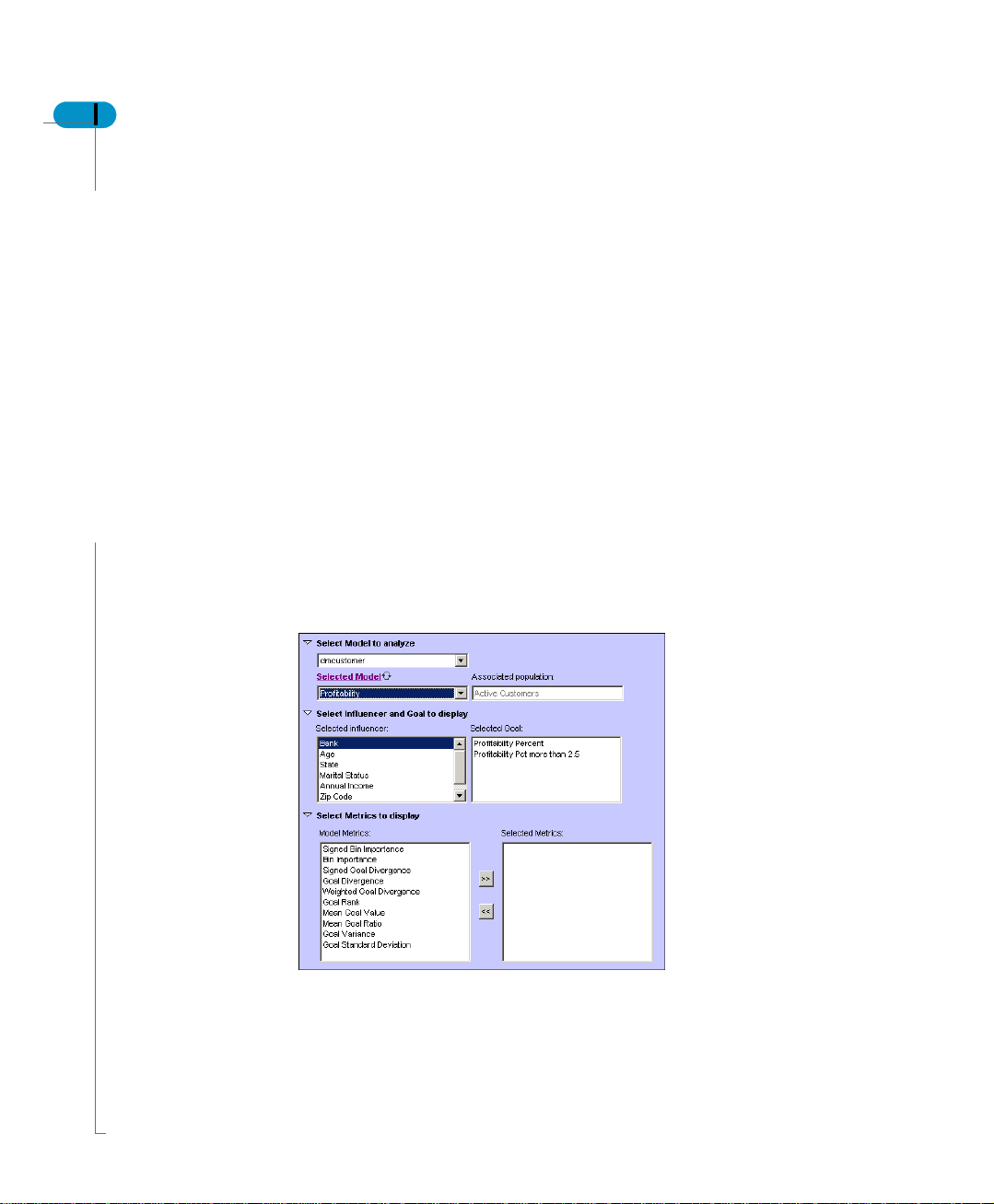
4. Select the metric that you want to be displayed.
These display the influencer level.
- Importance - Measures usefulness of Influencer for “predicting” goal values
- Obsolescence - If > 5, optimal binning may be obsolete (regeneration
needed)
- Net Relevance - Advanced metric calculated only at model regeneration
time
5. Select the display options.
You can choose to hide the influencers if the obsolete value is more than the
value defined. Check the box to do so and define the obsolete value.
6. You can sort the data in ascending or descending way, in order of metric for
a particular goal.
7. You can use a legend that can be linked to a document.
Influencer Analytics
Page 43

8. Click OK to display the analytics.
Predictive Analysis User’s Guide 43
Influencer analytics
Page 44
44 Predictive Analysis User’s Guide
Goal based influencer detail
Goal-Based Influencer Detail is an analytic that provides histogram display of
statistics calculated by the same modeling engine that supports the Key
Influencers analytic. It provides a detailed view of the relationship between a
single influencer variable and a single outcome or goal. The statistics can be
displayed based on explicit sub-divisions ("bins") of the influencer variable, or
based on sub-divisions that have been optimized for the goal.
Benefits:
• Identify "hot spots" (areas with unusually high or low statistic values) in the
relationship between a variable and an outcome measure or indicator.
• Profile variables that show up as important in Key Influencers, in terms of
descriptive statistics by sub-range or "bin."
!
Summary
Goal-Based Influencer Detail is an analytic that sheds light on the precise nature
of a variable's relationship to a key outcome or goal.
To define the analytic, follow the steps below:
1. Select the Subject Area from the drop-down list.
Influencer Analytics
2. Select the model from the drop-down list.
3. Select an Influencer under that model.
Page 45

Predictive Analysis User’s Guide 45
4. Select a goal from the model.
The selected goals are displayed in the analytic.
5. Select the metric that you want displayed.
These display the influencer level. Click the arrow key to move the selected
model metrics.
6. Select the display options.
You can sort the data in ascending or descending way, in order of bins or in
order of metric selected.
7. Click OK to generate the analytic.
Goal based influencer detail
Page 46

46 Predictive Analysis User’s Guide
Influencer gains chart
Influencer gains chart is an analytic that depicts the relationship between an
influencer variable and a binary outcome or goal, using a standard cumulative lift
graph. As with Influencer Detail and Goal-Based Influencer Detail, Influencer
Gains Chart profiles a variable by sub-range, or bin, but it does so in a manner
that takes into account both the outcome variable and bin frequency or count.
!
Benefits
• Identify "hot spots" (areas with unusually high or low statistic values) in the
relationship between a variable and an outcome measure or indicator-in a
manner that encompasses "% of population accounted for."
• Profile variables that show up as important in Key Influencers, in terms of
Cumulative Lift-the basis for "importance" calculation.
• Identify the best sub-ranges of a key influencer variable to use in segment
creation.
!
Summary
Influencer Gains Chart is an analytic that portrays tells you at a glance the nature
of a relationship between a variable and a key outcome indicator.
Influencer Analytics
Page 47

Predictive Analysis User’s Guide 47
EXAMPLE
Is the high importance of age as an influencer of monthly email campaign
response based (a) on spikes in one or two specific age bands, (b) on the
differential between two large age bands, or (c) on a gradual increase or
decrease in the response rate with increasing age?
Influencer gains chart
Page 48

48 Predictive Analysis User’s Guide
Models gains chart
Model Gains Chart is an analytic that depicts the relationship between the
combination of ALL influencer variables in a predictive model and a binary
outcome or goal, using a standard cumulative lift graph (used in database
marketing).
Benefits:
• Assess how much predictive power is contained in the sum total of a suite of
variables
• Determine the best cut-point to use for targeting based on values of a model
score variable (when used in conjunction with Individual List)
To define the analytic, follow the steps below:
1. Select the Subject Area from the drop-down list.
Influencer Analytics
2. Select the model from the drop-down list.
3. Select the associated population under the model.
Page 49

4. Select a goal from the model.
The selected goal is displayed in the analytic.
Predictive Analysis User’s Guide 49
The graph represents an analysis based on the existing population, this is not a
forecast. Based on it, you can identify the population more likely to respond
positively to the goal (here Annual income > 35k).
General in fo on the gra p h
• The random line is the baseline, actually it is just a reference to a random
response, 10 to 10, 50 to 50 etc.
• The optimal line represents the best response, it helps you out to compare
with the current response you get.
• For each bins, you can see the % cumulative response for the question, here
Annual income > 35k,
Reading the graph
• Start by reading the Y axis:
If you want 60% of good response for ex, start on the Y axis and then look for
the corresponding % of population to achieve that goal.
You see here that about 25 to 30% of the population, and it's in the orange
Models gains chart
Page 50

50 Predictive Analysis User’s Guide
bin, here Age [32;35].
So if you want to reach 60% of Annual Income > 35k, you will target the age
group [32-35] and since it's a cumulative response, you have to include the
first bin, here Age [27;32].
Usually, the idea here is to reach maximum gain with minimal % of population,
that's when you have for ex limited budget and resources.
!
Options to select in the edit part of the influencer gain chart generation
• Best gain orders the bins by displaying the best maximum lift response first
(for each bin)
• Model gain orders the bin based on the model results only
Influencer Analytics
Page 51

Variable profile box plot
Variable Profile Box Plot is an analytic that profiles the relationship between a
variable (character or numeric) and a numeric measure, using a standard box
plot graph. For each sub-range or "bin" of the selected variable, a box plot is
displayed that depicts the minimum, maximum, and quartiles (25th, 50th and
75th percentiles) of a profile measure's distribution. An alternative configuration
displays box plots based on mean and standard deviations.
Variable Profile Box Plot is used when it is important to understand how the
DISTRIBUTION of a profile measure varies by variable bin, for example, range,
variability and lopsidedness or "skew." By contrast, Influencer Detail is used for
profiling variables against multiple measures side-by-side based on a simple
aggregation such as mean.
!
Benefits
• Analyze how the range and distribution of a KPI varies for different values of
a focal attribute, so as to understand and improve consistency of
performance.
• Summarize the relationship between a focal attribute and profile or outcome
measure in a manner that teases out the influence of extreme values and
lopsided distributions.
Predictive Analysis User’s Guide 51
!
Summary
Variable Profile Box Plot tells you at a glance the nature of a relationship between
a focal variable and a profile measure in terms of averages, range and variability.
EXAMPLE
How is "sum of transaction fees" distributed for accounts of different ages?
To configure the Profile Box Plot, make sure to select the Population, Influencer,
Binning, Metric and Box Plot Configuration.
Variable profile box plot
Page 52

52 Predictive Analysis User’s Guide
To define the analytic, follow the steps below:
1. Select the Subject Area from the drop-down list.
2. Select the model from the drop-down list.
3. Select a population.
4. Select the Influencer and the binning from the list.
5. Select the Metric to be calculated.
6. Define the Display options.
- You can select the variability and view either by Range or Deviation. The
variability definitions are calculated automatically.
Influencer Analytics
Page 53

7. Click OK to generate the analytic.
Predictive Analysis User’s Guide 53
Variable profile box plot
Page 54

54 Predictive Analysis User’s Guide
Influencer detail
The influencer detail profiles an Influencer with respect to measures from the
universe and on performance metrics with respect to one or more outcomes
(“goals”). The influencer profile aggregates the count, frequency%, and the mean
(for example, mean of age for bin1 of age).
The influencer profile is based on user-defined binning or model-derived binning,
optimized for a selected goal.
To configure influencer details enter the following details.
Influencer Analytics
1. Select the Subject Area from the drop-down list.
2. Select the model from the drop-down list.
3. Select a population.
4. Select the Influencer and the binning from the list.
Page 55

Predictive Analysis User’s Guide 55
5. Select the Metric to be calculated.
6. You can sort in ascending or descending order.
7. Select a binning type.
8. Check if you wish the analytic to have prompts. You can check the box to
support default prompts.
Influencer detail
Page 56

56 Predictive Analysis User’s Guide
Influencer Analytics
Page 57

Lists and Forecasts
4
chapter
Page 58

58 Predictive Analysis User’s Guide
Overview
This chapter details the use of lists and forecasts in Predictive Analysis.
NOTE
Refer to Appendix for trouble shoot issues.
Lists and Forecasts
Page 59

Metric forecaster
Metric Forecaster forecasts a metric with error bands and auto-detection of
seasonal and other cyclical patterns. It predicts metric values for one or more
periods in the future. Metric Forecaster is updated automatically and requires
minimal knowledge to configure or use. Forecaster is an SVG analytic that
displays a past trend line for a selected metric and an N-point forecast into the
future. The basic configuration parameters required are:
• Focal metric with at least 20 periods of history
• How far into future to forecast
To define the analytic, follow the steps below:
Predictive Analysis User’s Guide 59
Metric forecaster
Page 60

60 Predictive Analysis User’s Guide
Defining Forecaster Parameters
1. Select a metric.
2. Click Select Metric.
A window allows you to select a metric.
3. Select if you want a Prompt every time the analytic refreshes.
Check the option button and enter the Prompt details.
4. Enter the Number of Periods you wish to forecast.
Defining Display Options
1. Enter the Title of the Analytic
2. Check if you wish to create a link in the legend.
3. Select the Width of the Error band.
4. Select the mode of Sampling Data.
Lists and Forecasts
If so enter the link path.
Liberal corresponds to 95% confidence interval around forecasted value and
Conservative corresponds to 99% confidence interval around forecast value.
Complete is the entire data set used as estimation for model generation;
Optimized is where three-fourths of the data set is used for estimation.
Page 61

Predictive Analysis User’s Guide 61
NOTE
The mode that you select is an important factor for model processing. Complete
mode is a good option for smaller data sets and metrics with trends. Optimized
works better for metric with cycles although the engine needs to detect at least
two cycles in the estimation data set.
5. Click OK to generate the analytic.
Metric forecaster
Page 62

62 Predictive Analysis User’s Guide
Individual list
Individual List is a facility for assembling a set of information for a group of
individuals that includes model scores and derived variables. As with other
analytics, Individual List refresh can be scheduled to occur at regular intervals.
The list can be displayed and stored in XML format.
!
Benefits
• Apply predictive models to the members of a set, or to individuals who fulfill
specific criteria for targeting, special handling, and/or integration with external
systems.
To define the analytic, follow the steps below:
Lists and Forecasts
1. Select the Subject Area.
2. Define the Population details.
- Select the Population
Page 63

Predictive Analysis User’s Guide 63
3. Click Next.
4. Define the Content details.
- Select the Objects and move it to the Selected side.
- You can add a column. You can add extra columns to define model score.
From the screen below, select the goal from the models.
- Define the number of rows you want to be displayed in the analytic.
Individual list
Page 64

64 Predictive Analysis User’s Guide
5. Click OK to generate the analytic.
Scores for numeric goals represent estimates of goal variable values based on
the selected model.
Scores for Boolean (True/False) goals represent estimated probabilities for the
individual having TRUE as the goal value based on the selected model.
Lists and Forecasts
Page 65

Appendix
chapter
Page 66

66 Application Foundation User’s Guide
Forecasting Algorithm
Choose the best combination of detrending algorithm, cyclicality and fluctuation
algorithm
Detrending
There are four type of trend:
• adjacent-point differencing (which means, that the best prediction for the
current value, is the last known)
• double differencing
• linear regression
• generalized regression on time.
So we compute each trend compared with the same signal. And we do that for
any type of data: meteorology, prices stock exchange, industrial process, or any
timestamp data, we apply the same algorithm.
After this step, we have four type of models (corresponding to each trend), and
the residuals corresponding to this model. These residuals have the following
definition: Res = Signal - Trend.
Decycling
Then, for each of these residual, we try to find one or more cyclicality (in the
current version, we try to find only one cyclicality).
After this step we have always four types of models, but for each of them, we
added found cyclicalities. So we get new residuals with the following definition:
NewRes = Signal - Trend - Cycles.
Fluctuations (envisaged for the v3)
Then, new residuals may have possible residual information. We call this residual
information, fluctuations.
Approximately, that means that one data may be an hidden linear combination of
one or more last data ( we can call that (memory phenomena). We determin e the
fluctuations of each residuals by using an auto-regressive model, which is
defined as follows:
X(t) = a(1) * X(t-1) + a(2) * X(t-2) + ... + a(n) * X(t-n).
Appendix
Page 67

Model type
Application Foundation User’s Guide 67
So, if we applied this definition to our residuals, we have:
NewRes = a(1) * NewRes(t-1) + a(2) * NewRes(t-2) + ... + a(n)
* NewRes(t-n).
At the end of this step, we get new residuals with the following definition:
NewRes2 = Signal - Trend - Cycles - Fluctuati ons.
If all is right, we find no residual information in these new residuals.
When all the phases are finished, we have four models, that are:
1. LastKnownValue + Cycles + Fluctuations
2. Double-differentiation + Cycles + Fluctuations
3. Linear Regression + Cycles + Fluctuations
4. Generalized Regression on Time + Cycles + Fluctuations
To choose the best model, compute all possible auto feed forecasts in validation
data set and compare these one to the real data (in v alidation). Choose the model
with the forecasts which are correlated with the real data, and which are
minimizing the mean squared error.
It is possible that the engine does not find any model: that means that there are
no correlated model.
Data type
Normally, as explained above, this algorithm is applied for any type of data:price
of the oil barrel, Paris temperatures, Co2 rate in Los Angeles atmosphere, or any
other.
Forecasting Algorithm
Page 68

68 Application Foundation User’s Guide
Universe configuration
To configure universe for Predictive analysis you need to make sure that the
following are defined:
1. The universe object defined should be referring to primary key of the table.
Appendix
Universe used for Data Mining can have only one 'SubjectKey=Y' per subject
area. For example, "customer" subject area has only one universe object, for
example, 'customer_id' with 'subjectKey = Y' defined.
The universe object that is defined with 'subjectKey=Y' should be referring to
primary key of the table.
You can have one and only one Universe object defined with 'SubjectKey=Y'
Page 69

Application Foundation User’s Guide 69
2. Specify outer join in the universe. This allows you to retrieve accurate sql from
WebIntelligence.
Example of an out join definition, "set_set_detail.id*=dmsales.customer_id".
where "*" means outer join definition.
Universe configuration
Page 70

70 Application Foundation User’s Guide
To check the population query
1. In AF system setup/trace, turn on SQL logging for every component. Then,
using the Create Analytic wizard, use the Individual List analytic with the
population that is failing. After the error appears in this analytic, return to the
log file and check for SQL errors. They are often related to joins or prompting.
2. In your metric universe, check to see that your dimension, fact (optional) and
set (optional) tables are properly joined together. Check the @Prompts on the
date fields if you are using a fact table and dynamic sets.
3. Test your population query using full client Business Objects. To do this, use
the metrics universe and select your key object and one filter. View the SQL.
Make sure that only a single Select appears as the AF Engine can't run multiselect queries. Run the query. If prompted for set_id or begin and end dates
(because you're using a dynamic set or fact table), enter those as well. Note
that you must enter the dates such that only one row per ID appears. If your
dates are too broad, you may get multiple rows per ID. This too will cause the
Individual List analytic to fail (because of key insert violations).
4. If the query runs without error or multi-select, the only remaining problem can
be the length of the key itself. If the integer key you are using is longer than
12 digits, the error encountered in step 1 may be an insert error. I've found
that by changing the data type of the ID field in the ci_indiv_num to BIGINT
(using SQL Server), I can overcome any insert errors related to the length of
my key.
Appendix
Page 71

To test derived variables
To test derived variables, follow the steps:
1. Create the Derived Variable.
2. Use the Individual List analytic again. This time, select your key and the
Derived Variable you created in step 1. If the Derived Variable displays
properly, it's syntax is correct. If not, edit the Derived Variable.
3. Repeat steps 1 and 2 for each Derived Variable. Once you've tested each
Derived Variable, you're ready to move onto Model Building.
NOTE
The query that is run for the model must always return a single row per key.
Because predictive models cannot do runtime query aggregation, the data used
with the metrics universe must already be summarized to the level of one row per
key value.
Application Foundation User’s Guide 71
To test derived variables
Page 72

72 Application Foundation User’s Guide
Model building
To build a model some tips to follow:
1. Create a simple model, using a small population (<1000 rows), one Influencer
and one Goal. If this runs successfully (and can be viewed by the Key
Influencer Analytic), increase the number of Influencers.
2. If you want to use the Influencer Detail or Lift Chart analy tics, one or more of
your goals must be a Derived Variable.
Appendix
Page 73

Glossary of Terms
appendix
Page 74

74 Predictive Analysis User’s Guide
The Glossary of terms provides a non-exhaustive list of commonly-used terms in
Predictive Analytics.
Term Definition
Binning Binning is a way of compressing the
Change Change is a subtraction between 2
Continuous Data Type Continuous is the default data type
Discarded Samples Discarded points are points that you
Gap Size Gap Size is the number of
Influencer An influencer is a variable whose
Joiners Joiners are those entities that currently
Metric A Metric is a mechanism that allows
Migration Migration is movement of individual
range of values for a variable into a
smaller number (for example, <=20) of
categories or "bins".
values of a single metric.
Generic formula is: Metric value
Current Period - Metric value Prior
period
corresponding to numeric variables.
may want to exclude from the baseline
window because they are out-ofcontrol.
measurements to be skipped between
two samples. This value is entered by
the user. The default value is 0.
ability is to anticipate goal values is of
interest.
reside in the set as of the most recent
refresh but did not reside in the set as
of the refresh prior to that.
you to track a measure over time for a
particular subset of a set.
customers from one set to another.
Glossary of Terms
Page 75

Predictive Analysis User’s Guide 75
Term Definition
Model A model is a configuration of a
calculation engine that controls what
the engine calculates and how.
Nominal Data Type Nominal variables are those whose
values are not inherently ordered.
Ordinal Data Type Ordinal variables are those that have
an ordering, but lack proportionality,
for example, the distance between
adjacent values is undefined (you
cannot do arithmetic with ordinal
variables).
Population A Population is a named query that
defines a group of interest.
Metric Metric is the mechanism that allows
you to create report analyses to track
customer set and subset behavior.
Rules Engine The rules engine allows you to
automatically identify, analyze, predict,
and act on a specific event.
Segmentation Segmentation is a way of partitioning
customers (or prospects, suppliers
etc.) into categories or ’sets’. Most
often they are mutually exclusive, but
they may also be overlapping.
Time Series Analysis Time-series analysis refers to the
unique ability of Application
Foundation to track the complex
details of millions of customer behavior
and their transactions in real-time, thus
allowing you to respond rapidly to
trends and take preventative action.
Time Stamp Time Stamp is the Date-time when the
sampling needs to start.
Variable A "variable" is simply a measured
characteristic or attribute.
Page 76

76 Predictive Analysis User’s Guide
Term Definition
Variable Data Variable data is continuous data that
Weighting Factor Weighting Factor determines the
Western Electric Rule The Western Electric rules (or Western
has been acquired through
measurement, for example length,
time, strength, temperature, pressure,
etc.
weights to be applied to samples. If the
factor=0.2 then 20% of the weight is
given to the most current sample and
80% to the past samples.
Electric Company rules, or WECO
rules) are used to determine if a
process is out of control and subject to
unexpected variation. Each Western
Electric rule identifies a situation that is
statistically very unlikely to be due to
random variation only.
Glossary of Terms
Page 77

Index
Predictive Analysis User’s Guide 77
A
Analytics
goal based influence r 44
benefits 44
summary 44
influencer detail 54
influencer gains chart 46
benefits 46
summary 46
key influencer 41
importance 41
net relevance 41
obsolescence 41
models gains
benefits 48
variable profile box plo t 51
benefits 51
summary 51
Appendix 65
Application Foundation documentation
Guides in PDF 6
obtaining more inform ati on about 6
audience 7
B
Binning
concept 11
create 23
edit 25
binning 22
C
Concepts
goal 11
goal based binning 11
influencer 12
model 11
variabl e 11
Configuration
derived variables 19
population 15
D
Derived variable
boolean 21
create new 20
date/numeric 21
usage 19
F
Forecasting algorithm 66
data 67
decycling 66
detrending 66
fluctuations 66
model 67
population query 70
test derived variabl es 71
G
grain 35
I
In the documentation 6, 7
Individual list 62
benefits 62
Index
Page 78

78 Predictive Analysis User’s Guide
Influencer
data types 12
continuous 12
nominal 12
ordinal 12
Influencer analytics
influencer gains chart 46
M
Metric forecaster 59
display opt ions 60
parameters 60
Model
metrics based 32
new 29
Model building
tips 72
Models 29
metric based
history 36
parameters 35
storage 35
models gains 48
more information 6
O
online guides 6
P
PDF guides 6
Population
Predictive analyti cs
Index
concept 11
create 16
overview 10
 Loading...