

User Guide: SAP Business Objects Advanced Analysis, edition for Microsoft
Office
■ Release 1.0 SP6
2010-12-12

Copyright
© 2010 SAP AG. All rights reserved.SAP, R/3, SAP NetWeaver, Duet, PartnerEdge, ByDesign, SAP
Business ByDesign, and other SAP products and services mentioned herein as well as their respective
logos are trademarks or registered trademarks of SAP AG in Germany and other countries. Business
Objects and the Business Objects logo, BusinessObjects, Crystal Reports, Crystal Decisions, Web
Intelligence, Xcelsius, and other Business Objects products and services mentioned herein as well
as their respective logos are trademarks or registered trademarks of Business Objects S.A. in the
United States and in other countries. Business Objects is an SAP company.All other product and
service names mentioned are the trademarks of their respective companies. Data contained in this
document serves informational purposes only. National product specifications may vary.These materials
are subject to change without notice. These materials are provided by SAP AG and its affiliated
companies ("SAP Group") for informational purposes only, without representation or warranty of any
kind, and SAP Group shall not be liable for errors or omissions with respect to the materials. The
only warranties for SAP Group products and services are those that are set forth in the express
warranty statements accompanying such products and services, if any. Nothing herein should be
construed as constituting an additional warranty.
2010-12-12

Contents
About this guide......................................................................................................................7Chapter 1
1.1
1.2
1.3
2.1
3.1
3.2
3.3
3.4
3.5
3.5.1
3.5.2
4.1
4.2
4.2.1
4.2.2
4.2.3
4.2.4
4.2.5
4.3
4.3.1
4.3.2
4.3.3
4.4
4.4.1
Who should read this guide?....................................................................................................7
User profiles............................................................................................................................7
About the documentation set...................................................................................................7
What's New.............................................................................................................................9Chapter 2
Changed features in Advanced Analysis 1.0 SP4.....................................................................9
Getting Started......................................................................................................................11Chapter 3
What is SAP BusinessObjects Advanced Analysis, edition for Microsoft Office? ..................11
Working with Advanced Analysis in Microsoft Excel 2007......................................................12
Working with Advanced Analysis in Microsoft PowerPoint 2007............................................16
Working with Advanced Analysis in Microsoft Excel 2003......................................................18
Enabling and disabling the Advanced Analysis Add-In.............................................................22
To enable or disable the Advanced Analysis Add-In in Microsoft Excel 2007 or Microsoft
PowerPoint 2007...................................................................................................................22
To enable or disable the Advanced Analysis Add-In in Microsoft Excel 2003..........................23
Creating Workbooks.............................................................................................................25Chapter 4
To insert a crosstab with data................................................................................................25
Defining style sets for crosstabs............................................................................................26
SAP cell styles.......................................................................................................................26
To apply a style set................................................................................................................28
To create a style set...............................................................................................................28
To share a style set................................................................................................................29
To delete a style set...............................................................................................................29
Inserting other components....................................................................................................29
To insert a dynamic chart.......................................................................................................30
To insert an info field..............................................................................................................30
To insert a filter......................................................................................................................31
Working with formulas............................................................................................................31
To create a formula................................................................................................................32
2010-12-123

Contents
4.4.2
4.4.3
4.4.4
4.4.5
4.4.6
4.4.7
4.4.8
4.4.9
4.4.10
4.4.11
4.4.12
4.4.13
4.4.14
4.4.15
4.4.16
4.5
4.5.1
4.6
4.6.1
4.6.2
4.6.3
4.6.4
SAPGetData..........................................................................................................................33
SAPGetDimensionDynamicFilter............................................................................................34
SAPGetDimensionEffectiveFilter............................................................................................34
SAPGetDimensionInfo...........................................................................................................35
SAPGetDimensionStaticFilter................................................................................................36
SAPGetDisplayedMeasures...................................................................................................36
SAPGetInfoLabel...................................................................................................................37
SAPGetMeasureFilter............................................................................................................37
SAPGetMember....................................................................................................................38
SAPGetSourceInfo................................................................................................................38
SAPGetVariable.....................................................................................................................39
SAPGetWorkbookInfo...........................................................................................................40
SAPListOfEffectiveFilters.......................................................................................................41
SAPListOfVariables...............................................................................................................41
SAPSetFilterComponent........................................................................................................42
Converting crosstab cells to formula......................................................................................43
To convert a crosstab to formula............................................................................................44
Working with macros.............................................................................................................44
SAPSetFilter..........................................................................................................................45
SAPSetVariable.....................................................................................................................46
SAPSetRefreshBehaviour......................................................................................................47
Syntax for entering values......................................................................................................48
5.1
5.2
5.2.1
5.2.2
5.2.3
5.3
5.3.1
5.3.2
5.4
5.4.1
5.4.2
5.4.3
5.5
5.5.1
5.5.2
5.6
5.6.1
Analyzing Data......................................................................................................................51Chapter 5
To open a workbook..............................................................................................................51
Analyzing data with the design panel......................................................................................52
The Analysis tab.....................................................................................................................52
The Information tab................................................................................................................53
The Components tab..............................................................................................................54
Prompting..............................................................................................................................57
To define prompt values.........................................................................................................58
To select workbook properties for prompting.........................................................................60
Filtering data .........................................................................................................................61
Filtering members...................................................................................................................62
Filtering measures..................................................................................................................66
To show/hide zeros in rows and columns...............................................................................69
Sorting data...........................................................................................................................70
To sort values........................................................................................................................70
To sort members....................................................................................................................71
Working with hierarchies........................................................................................................72
To include dimensions with hierarchies in an analysis.............................................................73
2010-12-124

Contents
5.6.2
5.7
5.7.1
5.7.2
5.8
5.8.1
5.8.2
5.9
5.9.1
5.9.2
5.9.3
5.10
5.11
6.1
7.1
7.2
To display single dimensions as hierarchy..............................................................................74
Calculating new measures .....................................................................................................75
To calculate a new measure based on available measures.....................................................75
To add a new measure based on one available measure........................................................76
Defining Conditional Formatting.............................................................................................78
To define a Conditional Format...............................................................................................78
To edit Conditional Formats...................................................................................................79
Defining the display of members, measures and totals...........................................................80
To define the members display...............................................................................................80
Defining the measures display................................................................................................80
Defining the totals display......................................................................................................83
To comment a data cell..........................................................................................................85
To save a workbook...............................................................................................................86
Creating Presentations.........................................................................................................87Chapter 6
To create a slide out of Microsoft Excel.................................................................................87
Settings.................................................................................................................................89Chapter 7
User settings.........................................................................................................................89
Support settings....................................................................................................................90
8.1
8.2
8.3
Troubleshooting....................................................................................................................93Chapter 8
To enable the Advanced Analysis Add-In after system crash (Microsoft Office 2007)............93
To enable the Advanced Analysis Add-In after system crash (Microsoft Excel 2003) .............93
Solving issues regarding the creation of Microsoft PowerPoint slides....................................94
More Information...................................................................................................................95Appendix A
2010-12-125

Contents
2010-12-126

About this guide
About this guide
1.1 Who should read this guide?
This guide is intended for users interested in building and analyzing workbooks using SAP
BusinessObjects Advanced Analysis, edition for Microsoft Office.
1.2 User profiles
There are three user profiles for SAP BusinessObjects Advanced Analysis, edition for Microsoft Office:
• Workbook Creator
Users who create and maintain workbooks based on SAP BEx queries, query views and SAP
NetWeaver BW InfoProvider.
• Data Analyst
Users who navigate through existing workbooks and analyze the data they contain. They can also
include workbooks in a Microsoft PowerPoint presentation and continue the analysis there.
• Administrator
IT specialists who install, configure and administer SAP BusinessObjects Advanced Analysis, edition
for Microsoft Office. They also assign security rights and authorizations to workbook creators and
analyzers.
If your existing profile needs to be modified, contact your IT administrator.
1.3 About the documentation set
The documentation set for SAP BusinessObjects Advanced Analysis, edition for Microsoft Office,
comprises the following guides and online help products:
2010-12-127

About this guide
Administrator Guide
The Administrator Guide contains detailed information that a user needs to install, configure and
administer the edition for Microsoft Office. The guide is available on the SAP Help Portal.
User Guide
The User Guide contains the conceptual information, procedures and reference material that a user
needs to create and analyze Microsoft Excel workbooks and Microsoft PowerPoint slides with the edition
for Microsoft Office. The guide is available on the SAP Help Portal.
Online Help
The online help contains the same information as the User Guide. It can be called by pressing the Help
button in the "Setting" group on the "Advanced Analysis" tab. For dialogs, you can access context
sensitive help by selecting F1.
FAQs
This document contains frequently asked questions regarding SAP BusinessObjects Advanced Analysis,
edition for Microsoft Office. It is available on the home page for Advanced Analysis, edition for Microsoft
Office, in the SAP Community Network.
Note:
SAP BusinessObjects Advanced Analysis, Web edition, although related very closely to SAP
BusinessObjects Advanced Analysis, edition for Microsoft Office, has its own documentation set,
including its own user guide and online help.
2010-12-128
What's New
What's New
The What's New chapter gives you an overview of the most important changes in Advanced Analysis,
edition for Microsoft Office, Support Packages. It is available as of Support Package 4 for every Support
Package that includes major changes in documentation.
A collection of all SAP notes for a Support Package is available on the home page for Advanced Analysis,
edition for Microsoft Office, in the SAP Community Network at http://www.sdn.sap.com.
Related Topics
• Changed features in Advanced Analysis 1.0 SP4
2.1 Changed features in Advanced Analysis 1.0 SP4
Advanced Analysis 1.0 SP4 introduces several changed features. The following sections briefly describe
the most important changes and where to find more information about them.
Adding comments to a data cell
With SP4, it is again possible to add comments to the data cells of a crosstab. You can edit the text in
comments and delete comments that you no longer need.
More information: User Guide / Online Help
Changed names for menu bars in Microsoft Excel 2003
The names of the menu bars of Advanced Analysis in Microsoft Excel has changed:
New NameOld Name
Advanced Analysis StandardStandard
Advanced Analysis ExtendedAnalysis&Design
More information: User Guide / Online Help
Life-Cycle Management documentation
The Life-Cyle Management documentation for the edition for Microsoft Office was enhanced.
More Information: Administrator Guide
2010-12-129

What's New
2010-12-1210

Getting Started
Getting Started
3.1 What is SAP BusinessObjects Advanced Analysis, edition for Microsoft Office?
SAP BusinessObjects Advanced Analysis, edition for Microsoft Office, is a Microsoft Office Add-In that
allows multidimensional analysis of OLAP sources in Microsoft Excel, MS Excel workbook application
design, and intuitive creation of BI presentations with MS PowerPoint. The Add-In is available for the
following Microsoft Office versions:
• Microsoft Excel 2007
• Microsoft PowerPoint 2007
• Microsoft Excel 2003
In the edition for Microsoft Office, you can use SAP BEx Queries, query views and SAP Netweaver BW
InfoProvider as data sources. The data is displayed in the workbook in crosstabs. You can insert multiple
crosstabs in a workbook with data from different sources and systems. If the workbook will be used by
different users, it is also helpful to add info fields with information on the data source and filter status.
Using the design panel, you can analyze the data and change the view on the displayed data. You can
add and remove dimensions and measures to be displayed easily with drag and drop. To avoid single
refreshes after each step, you can pause the refresh to build a crosstab. After ending the pause, all
changes are applied at once.
You can refine your analysis using conditional formatting, filter, prompting, calculations and display
hierarchies. You can also add charts to your analysis. If you want to keep a status of your navigation,
you can save it as an analysis view. Other users can then reuse your analysis.
For more sophisticated workbook design, the edition for Microsof Office contains a dedicated set of
functions in Microsoft Excel to access data and meta data of connected BW systems. There are also
a number of API functions available that you can use with the Visual Basic Editor, to filter data and set
values for BW variables.
Advanced Analysis, edition for Microsoft Office, must be installed on your local machine. You can
connect directly to a SAP NetWeaver BW system or you can connect via SAP BusinessObjects Enterprise
to include data sources. Typically, you use SAP BusinessObjects Enterprise to store and share workbooks
in productive environments, but in test systems, you can also directly connect to a BW system. Using
SAP BusinessObjects Enterprise enables you to save workbooks and presentations in a central
management system and to reuse analysis view in other applications, like Crystal Reports or Advanced
Analysis, Web edition.
2010-12-1211

Getting Started
3.2 Working with Advanced Analysis in Microsoft Excel 2007
In Microsoft Excel 2007, Advanced Analysis is available as a separate tab in the ribbon. The ribbon is
part of the Microsoft Office user interface above the main work area that presents commands and
options. Starting in the 2007 Microsoft Office system, this replaces menus and toolbars.
This guides describes procedures using the ribbon. Most of the options are also available via the context
menu.
The Advanced Analysis tab contains the following groups:
• Data Source
• Undo
• Data Analysis
• Display
• Insert Component
• Tools
• Design Panel
• Settings
The following tables describe the groups and their options.
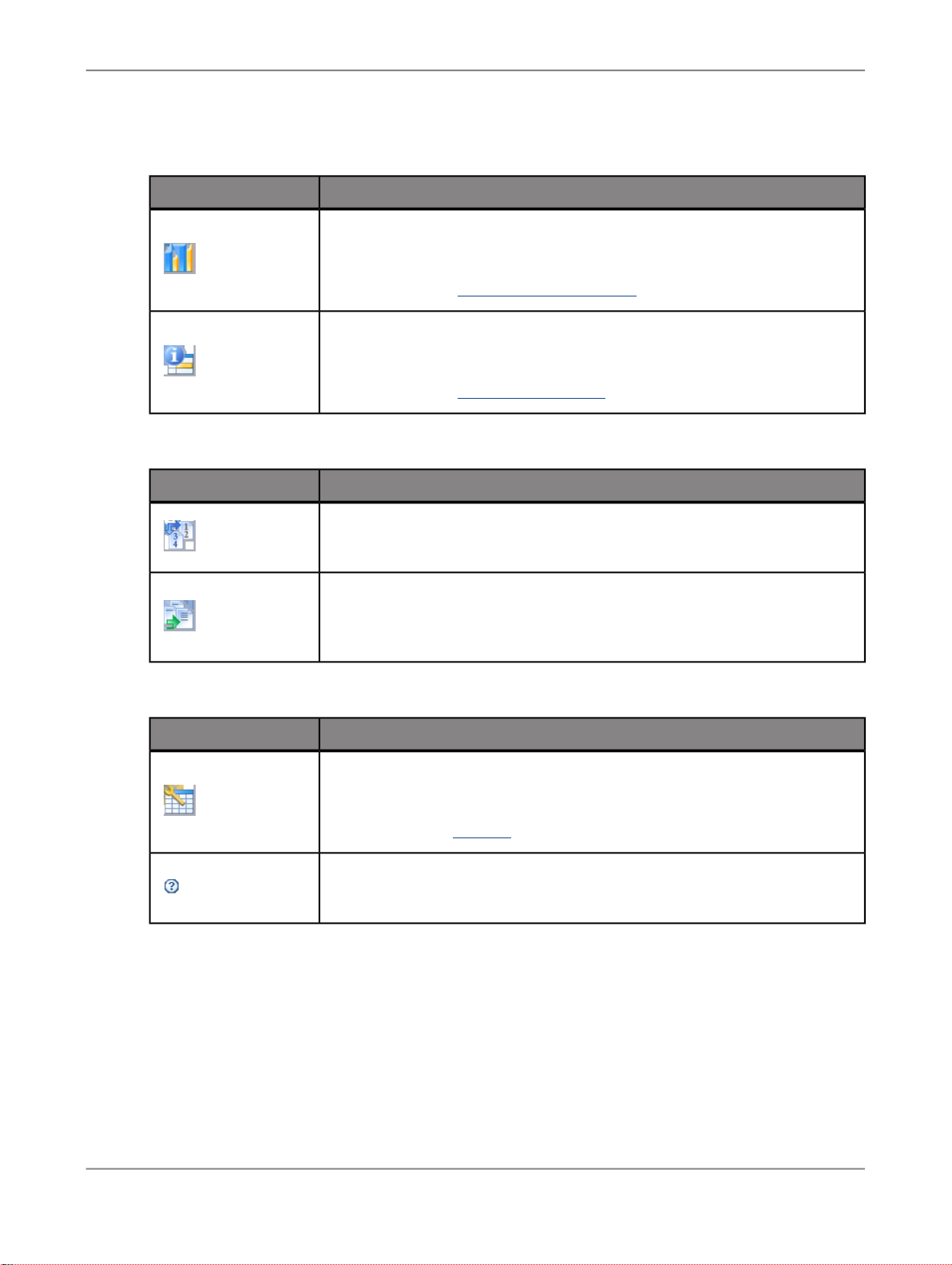
Data Source group
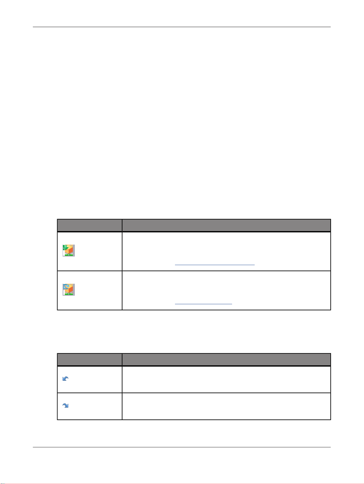
DescriptionIcon
Insert Data Source
Insert data from a source system into a crosstab.
More information: To insert a crosstab with data
Refresh All
Refresh all data sources.
More information: The Components tab
To open and save existing workbooks saved on the SAP BusinessObjects Enterprise Server, use the
corresponding options in the Microsoft Office button.
More Information: To open a workbook / To save a workbook
2010-12-1212

Getting Started
Undo group
Data Analysis group
DescriptionIcon
Undo
Undo last Advanced Analysis step.
Redo
Redo last Advanced Analysis step.
DescriptionIcon
Prompts
Enter values for query parameters and variables.
More information: Prompting
Filter
Define filter criteria for data.
More information:To filter data by measure / To filter data by member
Sort
Sort data.
More information: Sorting data
Hierarchy
Define hierarchy options such as expansion level and parent member positions.
More information: Working with hierarchies
Calculations
Define simple calculations (+,-,*,/) and dynamic calculations (for example,
ranking and cumulation.
More information: Calculating new measures
Swap Axes
Swap rows and columns.
2010-12-1213

Getting Started
Display group
DescriptionIcon
Conditional Formatting
Define rules for highlighting values using colors and symbols.
More information: To define a Conditional Format
Member Display
Configure display for members (key/text).
More information: To define the members display
Measure Display
Define display options for measures (for example, decimal places, scaling
factors and currencies).
More information: Defining the measures display
Totals
Configure display, position and calculation of totals.
More information: Defining the totals display
Insert Component group
DescriptionIcon
Chart
Insert dynamic chart.
More information: To insert a dynamic chart
Info Field
Insert information on data sources (for example, name and last data update).
More information: To insert an info field
Filter
Insert component for simple data filtering.
More information: To insert a filter
2010-12-1214

Getting Started
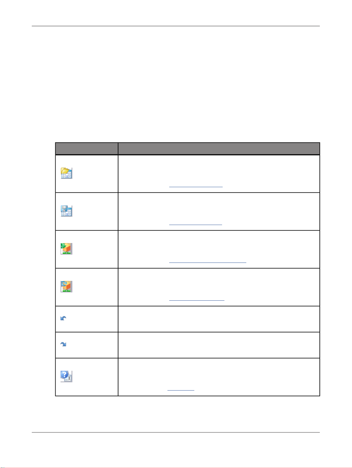
Tools group
Design Panel group
DescriptionIcon
Convert to Formula
Convert a crosstab into Excel formulas to retrieve the data.
More information: Converting crosstab cells to formula
Create Slide
Create Microsoft PowerPoint slide with data from selected crosstab.
More information: To create a slide out of Microsoft Excel
DescriptionIcon
Display
Settings group
Show/hide Design Panel
More information: Analyzing data with the design panel
Pause Refresh
Activate/deactivate automatic refresh after each navigation step in the Design
Panel.
More information: Analyzing data with the design panel
DescriptionIcon
Settings
Edit settings.
More information:Settings
Style
Manage crosstab styles.
More information: Defining style sets for crosstabs
Help
Launch help.
2010-12-1215
Getting Started
3.3 Working with Advanced Analysis in Microsoft PowerPoint 2007
In Microsoft PowerPoint 2007, Advanced Analysis is available as a separate tab in the ribbon. The
ribbon is part of the Microsoft Office user interface above the main work area that presents commands
and options. Starting in the 2007 Microsoft Office system, this replaces menus and toolbars.
The Advanced Analysis tab contains the following groups: :
• Data Source
• Undo
• Filter and Sort
• Display
• Insert Component
• Settings
The following tables describe the groups and their options.
Data Source group
DescriptionIcon
Insert Data Source
Insert data from a source system into a crosstab.
More information: To insert a crosstab with data
Refresh All
Refresh all data sources.
More information: The Components tab
To open and save existing presentations saved on the SAP BusinessObjects Enterprise Server, use
the corresponding options in the Microsoft Office button.
Undo group
DescriptionIcon
Undo
Undo last Advanced Analysis step.
Redo
Redo last Advanced Analysis step.
2010-12-1216
Getting Started
Filter and Sort group
DescriptionIcon
Prompts
Enter values for query parameters and variables.
More information:Prompting
Filter
Define filter criteria for data.
More information:To filter data by measureTo filter data by member
Sort
Sort data.
More information:Sorting data
Display group
Hierarchy
Define hierarchy options such as expansion level and parent member positions.
More information: Working with hierarchies
DescriptionIcon
Member Display
Configure display for members (key/text).
More information: To define the members display
Measure Display
Define display options for measures (for example, decimal places, scaling
factors and display currency).
More information: Defining the measures display
Totals
Configure display, position and calculation of totals.
More information: Defining the totals display
2010-12-1217
Getting Started
Insert Component group
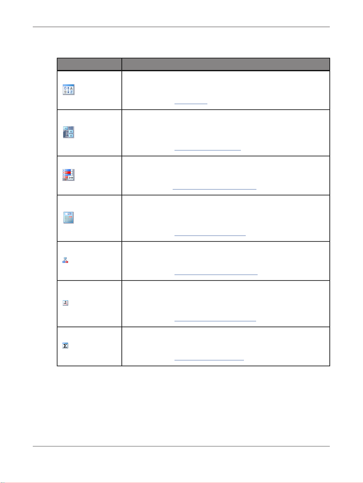
Tools group
DescriptionIcon
Chart
Insert dynamic chart.
More information: To insert a dynamic chart
Info Field
Insert information on data sources (for example, name and last data update).
More information: To insert an info field
DescriptionIcon
Fit Table
Settings group
Abbreviate a table to fit one slide, or split the table across multiple slides.
Move to
Move the selected Advanced Analysis object (table, chart or info field) from
its current location to different slide in the presentation.
DescriptionIcon
Settings
Edit settings.
More information:Settings
Help
Launch help.
3.4 Working with Advanced Analysis in Microsoft Excel 2003
2010-12-1218
Getting Started
In Microsoft Excel 2003, Advanced Analysis is available as separate item in the menu. You can access
all options with the menu. You can also include two toolbars: Advanced Analysis Standard and Advanced
Analysis Extended. These toolbars contain most of the available options.
To toggle between showing and hiding a toolbar, choose View > Toolbars and select the toolbar
name. A checkmark beside a toolbar name indicates that the toolbar is currently showing.
This guides describes procedures using the toolbars. Most of the options are also available via the
context menu.
Advanced Analysis Standard toolbar
The Advanced Analysis Standard toolbar contains the following options:
DescriptionIcon
Open Workbook
Opern workbook from SAP BusinessObjects Enterprise Server.
More information: To open a workbook
Save Workbook
Save workbook to SAP BusinessObjects Enterprise Server.
More information: To save a workbook
Insert Data Source
Insert data from a source system into a crosstab.
More information: To insert a crosstab with data
Refresh All
Refresh all data sources.
More information: The Components tab
Undo
Undo last Advanced Analysis step.
Redo
Redo last Advanced Analysis step.
Prompts
Enter values for query parameters and variables.
More information:Prompting
2010-12-1219
Getting Started
DescriptionIcon
Charts
Insert dynamic chart.
More information: To insert a dynamic chart
Info Field
Insert information on data sources (for example, name and last data update).
More information: To insert an info field
Filter
Insert component for simple data filtering.
More information: To insert a filter
Convert to Formula
Convert a crosstab into Excel formulas to retrieve the data.
More information:Converting crosstab cells to formula
Display
Show/hide Design Panel
More information: Analyzing data with the design panel
Pause Refresh
Activate/deactivate automatic refresh after each navigation step in the Design
Panel.
More information: Analyzing data with the design panel
Advanced Analysis Extended toolbar
The Advanced Analysis Extended toolbar contains the follwing options:
DescriptionIcon
Filter
Define filter criteria for data.
More information:To filter data by measureTo filter data by member
2010-12-1220
Getting Started
DescriptionIcon
Sort
Sort data.
More information: Sorting data
Hierarchy
Define hierarchy options such as expansion level and parent member positions.
More information: Working with hierarchies
Conditional Formatting
Define rules for highlighting values using colors and symbols.
More information:To define a Conditional Format
Calculations
Define simple calculations (+,-,*,/) and dynamic calculations (for example,
ranking and cumulation.
More information: Calculating new measures
Member Display
Configure display for members (key/text).
More information: To define the members display
Measure Display
Define display options for measures (for example, decimal places, scaling
factors and currencies).
More information: Defining the measures display
Totals
Configure display, position and calculation of totals.
More information: Defining the totals display
Advanced Analysis menu
The Advanced Analysis menu contains all options that are available as icons in the toolbars plus the
following opitions:
• Styles
• Settings
2010-12-1221

Getting Started
More information:Settings
• Help
3.5 Enabling and disabling the Advanced Analysis Add-In
After installing Advanced Analysis, edition for Microsoft Office, the Add-In is available in the menu every
time you open Microsoft Excel or Powerpoint. You can disable the Add-In so that it is not available when
you open a Microsoft Excel or Powerpoint file.
Related Topics
• To enable or disable the Advanced Analysis Add-In in Microsoft Excel 2007 or Microsoft PowerPoint
2007
• To enable or disable the Advanced Analysis Add-In in Microsoft Excel 2003
3.5.1 To enable or disable the Advanced Analysis Add-In in Microsoft Excel 2007 or
Microsoft PowerPoint 2007
Depending on how Advanced Analysis has been configured, you can enable or disable the Advanced
Analysis Add-In in Microsoft Excel 2007 and Microsoft PowerPoint 2007.
1.
Open any Microsoft Excel or Microsoft PowerPoint file.
2.
Press the Microsoft Office Button.
3.
In Microsoft Excel, select Excel Options. In Microsoft PowerPoint, select PowerPoint Options.
4.
In the "Excel Options" dialog box and the "PowerPoint Options" dialog box in the categories pane,
select Add-Ins.
5.
In the Manage box, select COM Add-Ins.
6.
Press Go....
7.
In the "COM Add-Ins" dialog box, activate or deactivate the option Advanced Analysis.
8.
Press OK.
If you enable the Advanced Analysis Add-In, it is always available when you open Microsoft Excel 2007
or Microsoft PowerPoint 2007.
If you disable the Advanced Analysis Add-In, it is not available when you open Microsoft Excel 2007
or Microsoft PowerPoint 2007. To work with SAP BusinessObjects Advanced Analysis, edition for
Microsoft Office, you have to open the program directly.
2010-12-1222

Getting Started
3.5.2 To enable or disable the Advanced Analysis Add-In in Microsoft Excel 2003
Depending on how Advanced Analysis has been configured, you can enable or disable the Advanced
Analysis Add-In in Microsoft Excel 2003.
1.
Open any Microsoft Excel file.
2.
On the View menu, choose Toolbars > Customize... .
3.
Select the Commands tab.
4.
In the Categories box, select Tools.
5.
In the Commands box, select COM Add-Ins and drag it to a toolbar.
6.
On the toolbar, select COM Add-Ins to see the list of available add-ins.
Note:
The Advanced Analysis Add-In is only available in this list, if your administrator set the corresponding
parameter in the registry. If you cannot see the Advanced Analysis Add-In, contact your administrator.
7.
Activate or deactivate the option Advanced Analysis.
8.
Press OK.
If you enable the Advanced Analysis Add-In, it is always available when you open Microsoft Excel 2003.
If you disable the Advanced Analysis Add-In, it is not available when you open Microsoft Excel 2003.
To work with SAP BusinessObjects Advanced Analysis, edition for Microsoft Office, you have to open
the program directly.
2010-12-1223

Getting Started
2010-12-1224

Creating Workbooks
Creating Workbooks
4.1 To insert a crosstab with data
To add a crosstab with data to a workbook, you select a data source in a SAP NetWeaver BW system.
You need the appropriate authorizations for SAP BusinessObjects Enterprise and the relevant SAP
NetWeaver BW systems to insert a data source in a workbook. For more information, contact your IT
administrator.
You can insert SAP BEx Queries, query views and SAP Netweaver BW InfoProvider as data sources.
These data sources are stored in a SAP NetWeaver BW system. You can add multiple crosstabs to
worksheet or workbook. The crosstabs can contain data from the same data source or from different
sources. You can also use data sources that are stored in different systems in one workbook.
1.
Select the cell in the worksheet where the crosstab with the data from the selected data source
should be inserted.
2.
Select Insert Data Source.
The "Log on to BusinessObjects Enterprise" dialog box appears.
3.
Enter your User, Password and the WEB Service URL to BusinessObjects Enterprise.
Note:
By selecting Skip you can log on to a BW system directly without using BusinessObjects Enterprise.
Continue with step 8 if you use this log on.
4.
Optional step: Enter System and Authentication.
You will normally not be asked to supply this information. However, if you are asked to log on to a
special Central Management System (CMS), you can add these two additional fields to the dialog
box by selecting Options. Enter the name of your Central Management System in the System field
and the authentication type in the Authentication field.
5.
Press OK.
The "Select Data Source" dialog box appears.
6.
Select a connection in the Show Connections list:
• If you select All, all available systems, Cubes / InfoProvider and Query / Query views on SAP
BusinessObjects Enterprise are displayed.
• If you select System, all available systems on SAP BusinessObjects Enterprise are displayed.
• If you select Cube / InfoProvider, all available Cubes and InfoProvider on SAP BusinessObjects
Enterprise are displayed.
• If you select Query / Query View, all available Queries and query views on SAP BusinessObjects
Enterprise are displayed.
2010-12-1225

Creating Workbooks
• If you select Local System, all systems in your local "SAP Logon" are displayed.
7.
Select a system and Next.
To select a Query, query view or InfoProvider directly, double-click the object you want to select.
The "Logon to System" dialog box appears.
8.
Enter Client, User and Password in the fields and press OK.
If you want to specify the system language, select Options and enter the language in the Language
field.
9.
Select a data source in the Select Data Source box and press OK.
On the Folders tab, you can navigate in the Roles or InfoAreas views to find a data source.
On the Search tab, you can search for the description or technical name of a data source. To retrieve
data sources that begin with a specific string, you can type * after a partial string.
A new crosstab with the data of the selected data source is inserted in the worksheet. You can now
analyze the data and change the displayed data set according to your needs. You can also add other
components to your anaylsis, for example charts.
4.2 Defining style sets for crosstabs
A style set is a collection of Microsoft Excel cell styles that is applied by Advanced Analysis to format
the cells of a crosstab. Whenever you insert a new crosstab in a workbook, the styles in the current
default style set are used to format the crosstab cells. You can change the applied style set in your
analysis. With Advanced Analysis, the following style sets and their cell styles are installed:
• SAP Tradeshow Plus
• SAP Blue
• SAP Black&White
By modifying the cell styles of these style sets, you can create your own style sets and share them with
other users.
4.2.1 SAP cell styles
SAP standard styles
SAP standard styles are availabe after the installation of the Add-In. You can modify them in the Styles
group on the Home tab of Microsoft Excel. They affect the formatting as described in the following table:
2010-12-1226

Creating Workbooks
Cell
Cell
el1-9
DescriptionStyle Name
Format for dimension header cells.SAPDimensionCell
Format for member cells (non-hierarchical dimensions).SAPMemberCell
Format for hierachical member cells (even levels 0, 2, ...).SAPHierarchyCell
Format for hierarchical member cells (odd levels 1, 3, ...) .SAPHierarchyOdd-
Format for member total cells.SAPMemberTotal-
Format for data cells.SAPDataCell
Format for data total cells.SAPDataTotalCell
Format for highlighted cells due to conditional formats (rule priorities 1-9).SAPExceptionLev-
Format for highlighted data cells (as per query definition).SAPEmphasized
SAPBorder
Format for borders around a crosstab and between header/member and data
cells (format for left border is taken).
SAP custom styles
The following SAP custom styles are not availabe after the installation of the Add-In, but you can create
them in the Styles group on the Home tab of Microsoft Excel. They affect the formatting as described
in the following table:
DescriptionStyle Name
Format for member cells on columns (overriding SAPMemberCell).SAPMemberCellX
Format for member total cells on columns (overriding SAPMemberTotalCell).SAPMemberTotal-
CellX
SAPHierarchyCellX
Format for hierarchical member cells on columns, even levels (overriding SAPHierarchyCell).
SAPHierarchyOddCellX
SAPHierarchyCell0-9
SAPHierarchyCellX0-9
Format for hierarchical member cells on columns, odd level (overriding SAPHierarchyOddCell).
Format for hierarchical member cells on specific level (overriding SAPHierarchyCell
and SAPHierarchyOddCell).
Format for hierarchical member cells on specific level on columns (overriding
SAPHierarchyCellX and SAPHierarchyOddCellX).
Example: SAPMemberCellX
The column headings are defined as SAPMemberCell. If you want a different format for these cells
than for member cells in rows, you can duplicate the SAPMemberCell, name it SAPMemberCellX and
2010-12-1227

Creating Workbooks
change the format definition. If you save this as style set, the member cells in column headings are
displayed in the new defined format. The member cells in rows continue to be displayed as defined
in the SAPMemberCell style.
4.2.2 To apply a style set
You can apply one of the SAP style sets or any new defined style set to a workbook.
1.
Choose Styles > Apply Style Set....
The "Apply Style Set" dialog box appears.
2.
In the list box, selet the style set you want to apply.
3.
Select the Set as Default check box if the style set should be applied as default in your workbooks.
The default style set is used when you open a new workbook and insert a data source.
4.
Press OK.
The style set is applied to all crosstabs in your workbook.
4.2.3 To create a style set
Based on availabe cell styles, you can define a new style set. You change the cell styles according to
your needs using the Microsoft Excel style functionality. You can then save the new defined styles in
a style set.
1.
On the Home tab, in the Styles group, choose Cell Styles.
Note:
In Microsoft Excel 2003, you can find the cell styles by choosing Format > Styles in the menu.
The available cell styles are listed.
2.
Modify the existing cell styles or create new ones according to your needs.
3.
On the Advanced Analysis tab, in the Settings group, choose Styles > Save Style Set....
The "Save Style Set" dialog box appears.
4.
Enter a Style Set Name.
5.
Select the Set as Default check box if the style set should be applied as default in your workbooks.
The default style set is used when you open a new workbook and insert a data source.
6.
Press OK.
The new defined style set is created and availalbe in the list of style sets that can be applied to a
workbook.
2010-12-1228

Creating Workbooks
4.2.4 To share a style set
You can share a style set with other users by exporting the style set to a local fileshare. Other users
can import the style set and use it for the analysis.
1.
Apply the style set that you want to export.
2.
Choose Styles > Export Style Set....
3.
Save the style set as XML format.
The XML file contains the cell styles of the three SAP style sets and your currently applied style set.
4.
Choose Styles > Import Style Set....
5.
Select a style file from the server and press Open.
6.
Save the imported styles as new style set.
You have exported a style set to be used by other users and / or you have imported a style set to use
it in your analysis.
4.2.5 To delete a style set
You can delete all user-defined style sets. The standard SAP style set that is installed with the Add-In
can not be deleted.
1.
Choose Styles > Delete User Style Set.
The "Delete User Style Set" dialog box appears.
2.
In the list box, selet the style set you want to delete.
3.
Press OK.
The style set is deleted and no longer available in the list of style sets that can be applied to a workbook.
4.3 Inserting other components
In addition to crosstabs, you can add the following components to your analysis:
• Charts to provide a graphical presentation of the data in the crosstab.
• Info fields to provide metadata information.
• Filters to provide simplified filtering for end users.
2010-12-1229

Creating Workbooks
4.3.1 To insert a dynamic chart
1.
Select a cell of the crosstab that you want to visualize in a chart.
By inserting a chart with Advanced Analysis, the data of the entire crosstab is visualized in the chart.
If you want to visualize only a subset of the crosstab data, you can use Microsoft Excel functionality.
2.
Press the Chart button.
The chart is added to the analysis. You can position it in the worksheet using drag and drop.
3.
Modify the chart.
To modify the chart, you can use Microsoft Excel options for charts. For example, you can change
the chart type or define a data range for the chart.
4.
You can move the chart to another worksheet in the workbook.
On the Component tab in the design panel, select the chart you want to move, and open the Move
to dialog. Select the sheet that should contain the chart and press OK.
The chart is added to the analysis according to your configuration. The chart is updated automatically
when you change the displayed data in the crosstab.
4.3.2 To insert an info field
You can insert information fields to provide additional information on data displayed in the workbook
sheets.
1.
Select an empty cell where you want to place the info field.
2.
Select the info field you want to insert.
• Choose Info Field and one of the listed fields: Data Source Name, Last Data Update, Key Date,
Effective Filters, Variables. If you want to insert other info fields, use the second option.
The info field is added to worksheet. If you use more than one data source in your analysis, you
are prompted to select a data source.
• You can also drag and drop the info fields from the Information tab in the design panel to a cell
in the worksheet.
Select the data source on the top of the tab and drag and drop the information you want to insert
as info field. For dynamic info fields (filters and variables), you have to use the first option.
The info fields are inserted with label and source information. The functions used for the formulas are
SAPGetInfoLabel and SAPGetSourceInfo. The formulas are created automatically.
2010-12-1230

Creating Workbooks
4.3.3 To insert a filter
You can insert a filter component to your analysis to simplify the filtering. This helps you to quickly
change the view of the displayed data, for example to different periods of time.
1.
Select an empty cell where you want to place the filter component.
2.
Choose Filter and select one of the listed dimensions to insert a filter component for this dimension.
The dimension name and a filter component formula are inserted in the worksheet. The functions
used for the formulas are SAPGetDimensionInfo and SAPSetFilterComponent. The formulas are
created automatically.
3.
Optional Step: Specify the filter component formula.
The formula that is inserted automatically, allows the user to select multiple members for filtering.
It looks like this: =SAPSetFilterComponent("DS_2"; "0CALYEAR";"ALL").
You can add one of the following parameters to the formula: SINGLE, MULTIPLE,
LOWERBOUNDARY, UPPERBOUNDARY to specify the filtering options. If you add the parameter
SINGLE, the user can only select one member for filtering. The formula looks like this:
=SAPSetFilterComponent("DS_2"; "0CALYEAR";"ALL";"SINGLE").
You can also insert filter components to enable a range selection. Insert two filter components for
the same dimension and add to one the parameter LOWERBOUNDARY and to the other the
parameter UPPERBOUNDARY. You can now filter for the lower and upper bounds of a range.
4.
Optional step: Format the filter component.
You can use the formatting options of Microsoft Excel to format cells of the filter component.
5.
Select the filter icon to define a filter.
All tables on the current sheet that contain this dimension, will be filtered according to the selected
filter. On the Components tab in the design panel, you can define which tables should be affected
if not all tables should be filtered accordingly.
The filter is added to the analysis according to your configuration.
Related Topics
• SAPGetDimensionInfo
• SAPSetFilterComponent
4.4 Working with formulas
In Advanced Analysis, edition for Microsoft Office, you can use the standard functions of Microsoft Excel
to build formulas. The Add-in also contains an own set of functions that you can use to build formulas.
2010-12-1231

Creating Workbooks
You can use these functions to include data and meta data of used data sources into your analysis.
For example, you can insert information fields on data source properties, display the measure filter or
list the variables of a data source. With the SAPGetData function, you can also define measure values
for certain member combinations.
A Microsoft Excel formula for Advanced Analysis consists of a function and references to the data
source, measures and/or dimensions. You can use the text or the key of an object to use it as reference.
You can also use a cell value like B10 as reference.
The formula alias of a data source is displayed and can be changed in the data source properties on
the Components tab in the design panel. For measures, dimensions and their members text references
are better to read, but if you want to create a multi-language enabled analysis or there are duplicate
texts in the meta data of your data source, you should reference these objects with their keys.
Advanced Analysis functions
The following functions are available in the Advanced Analysis category:
• SAPGetData
• SAPGetDimensionDynamicFilter
• SAPGetDimensionEffectiveFilter
• SAPGetDimensionInfo
• SAPGetDimensionStaticFilter
• SAPGetDisplayedMeasures
• SAPGetInfoLabel
• SAPGetMeasureFilter
• SAPGetMember
• SAPGetSourceInfo
• SAPGetVariable
• SAPGetWorkbookInfo
• SAPListOfEffectiveFilters
• SAPListOfVariables
• SAPSetFilterComponent
4.4.1 To create a formula
To create a formula with Advanced Analysis functions:
1.
Select the cell in which you want to enter the formula.
2.
To start the formula with a function, press the Insert Function button on the formula bar.
The "Insert Function" dialog box appears.
3.
Select Advanced Analysis in the Select a category box.
4.
Select a function.
5.
Press OK.
The "Function Arguments" dialog box appears.
2010-12-1232

Creating Workbooks
6.
Enter the arguments.
To enter cell references as an argument, press the Collapse Dialog button (which temporarily hides
the dialog box), select the cells on the worksheet, and then press the Expand Dialog button.
7.
When you complete the formula, press OK.
4.4.2 SAPGetData
The function returns the measure value for a specific dimension member combination.
The formula can only return values for member combinations that are part of the current navigation
state of the data source. To be part of the navigation state, the member combinations must be used in
rows, columns or as background filter. If you filter a dimension, you can only return values for member
combinations that the filter contain. For example, if the navigation state of the data source displays the
dimension Region in rows and the measures Sales Volume in columns, you can create a formula to
return a value for a particular region, but you can not return a value for a special customer, even if
customer information is available in the data source. To be able to return values for a special customer,
you have to add the dimension to the navigation state, for example as background filter.
This formula consists of at least 3 parameters and is made up of the following arguments:
• Data Source
Enter the formula alias for the data source. You can set the alias when configuring the data source
on the Components tab in the design panel.
• Measure
Enter the name of measure, for example "Incoming Orders".
• Member combination
There are two forms to enter the member combination:
• Enter one parameter as member combination, for example "Region=France;Product=Services"
. This form is used for converting to formula.
• Enter several parameters as member combination, for example "Region";"France";"Product";"Ser
vices". This form can only be entered manually. It is recommended for member combinations
that use cell references.
Example: 3 Parameters formula
Cell H20: =SAPGetData("Data_Provider_1", "Incoming Orders" , "Region=France;Product=Services")
The data for the value in this cell come from data source Data_Provider_1. The name of the measure
is Incoming Orders. The member combination is France and Services. The formula in cell H20 therefore
uses the data from Data_Provider_1 to calculate the incoming orders for Region France and Product
Services. If you change France to Germany in the formula, the incoming orders for Germany and
Services are displayed in cell H20.
2010-12-1233

Creating Workbooks
Example: >3 Parameters formula with cell reference
Cell H20: =SAPGetData("Data_Provider_1", "Incoming Orders" , "Region";"B10";"Product";"Services")
The data for the value in this cell come from data source Data_Provider_1. The name of the measure
in Incoming Orders. The member combination is the region that is entered in cell B10 and Services.
For example, if you enter Spain in cell B10. the formula in cell H20 uses the data from Data_Provider_1
to calculate the incoming orders for Region Spain and Product Services. If you change Spain to France
in the cell B10, the incoming orders for France and Services are displayed in cell H20.
4.4.3 SAPGetDimensionDynamicFilter
The function returns the dynamic filter of a dimension. Dynamic filters are defined by the user.
This formula consists of 3 parameters and is made up of the following arguments:
• Data Source
Enter the formula alias for the data source. You can set the alias when configuring the data source
on the Components tab in the design panel.
• Dimension
Enter the technical name of the dimension.
• Member Display
You can enter TEXT or KEY to define how the filtered members should be displayed in the workbook.
Example:
Cell F20: =SAPGetDimensionDynamicFilter("DS_1";"0DIVISION";"TEXT")
You add a filter for dimension 0DIVISION and the following members are displayed in the analysis:
Paints, Lighting, Foods. If you enter the formula in cell F20, the three filtered members are displayed
in cell F20 as text..
4.4.4 SAPGetDimensionEffectiveFilter
The function returns all effective filters of a dimension: Dynamic filters that are defined by the user,
static filters that are defined in the underlying source, and filters by measure that are defined for the
selected dimension.
This formula consists of 3 parameters and is made up of the following arguments:
2010-12-1234

Creating Workbooks
• Data Source
Enter the formula alias for the data source. You can set the alias when configuring the data source
on the Components tab in the design panel.
• Dimension
Enter the technical name of the dimension.
• Member Display
You can enter TEXT or KEY to define how the filtered members should be displayed in the workbook.
Example:
Cell F20: =SAPGetDimensionEffectiveFilter("DS_1";"0DIVISION";"TEXT")
If you enter the formula in cell F20, the members of 0DIVISION that are currently filtered by the user,
the static filters that are defined in the data source and the filters by measure for this dimension are
displayed in cell F20 as text. If no static filters are defined for the data source, only the dynamic filter
members and filters by measure are displayed.
4.4.5 SAPGetDimensionInfo
The function returns the name of a dimension or the name of an active hierarchy.
This formula consists of 3 parameters and is made up of the following arguments:
• Data Source
Enter the formula alias for the data source. You can set the alias when configuring the data source
on the Components tab in the design panel.
• Dimension
Enter the technical name of the dimension.
• Property Name
You can enter the follwoing property names:
• NAME
• ACTIVEHIERARCHY
Example:
Cell F20: =SAPGetDimensionInfo("DS_1";"0DIVISION";"NAME")
If you enter the formula in cell F20, the name of dimension 0DIVISION is displayed in cell F20.
2010-12-1235

Creating Workbooks
4.4.6 SAPGetDimensionStaticFilter
The function returns the static filter of a dimension. Static filters are defined in the underlying source
and cannot be changed by the user.
This formula consists of 3 parameters and is made up of the following arguments:
• Data Source
Enter the formula alias for the data source. You can set the alias when configuring the data source
on the Components tab in the design panel.
• Dimension
Enter the technical name of the dimension.
• Member Display
You can enter TEXT or KEY to define how the filtered members should be displayed in the workbook.
Example:
Cell F20: =SAPGetDimensionStaticFilter("DS_1";"0MATERIAL";"KEY")
If you enter the formula in cell F20, the static filter of dimension 0MATERIAL is displayed in cell F20.
4.4.7 SAPGetDisplayedMeasures
The function returns a list of all measures displayed in the analysis as text.
This formula is made up of the following argument: Data Source.
Enter the formula alias for the data source. You can set the alias when configuring the data source on
the Components tab in the design panel.
Example:
Cell G10: =SAPGetDisplayedMeasures("DS_1")
If you enter the formula in cell G10, all measures that are currently displayed in the crosstab are listed
in cell G10. If you add or remove a measure from the crosstab, the list in cell G10 is updated
accordingly.
2010-12-1236

Creating Workbooks
4.4.8 SAPGetInfoLabel
The function returns the language dependant label of a specific info field. The available property names
correspond to the info fields that are available for workbook and data sources on the Information tab
in the design panel. Using this functions, the info field labels are displayed in the selected UI language.
The info field values can be inserted with function SAPGetWorkbookInfo and SAPGetSourceInfo.
This formula is made up of the following argument: Property Name.
For workbook related info fields, you can enter the follwoing property names:
• WorkbookName
• CreatedBy
• CreatedAt
• LastChangedAt
• LastRefreshedAt
• LogonUser
For data source related info fields, you can enter the follwoing property names:
• DataSourceName
• LastDataUpdate
• KeyDate
• QueryTechName
• QueryCreatedBy
• QueryLastChangedBy
• QueryLastChangedAt
• InfoProviderTechName
• InfoProviderName
• System
Example:
Cell D20: =SAPGetInfoLabel("System")
The label of the info field is displayed in the selected UI language, for example in English: System.
4.4.9 SAPGetMeasureFilter
The function returns a list of all filtered measures and their rules defined for a data source.
This formula is made up of the following argument: Data Source.
2010-12-1237

Creating Workbooks
Enter the formula alias for the data source. You can set the alias when configuring the data source on
the Components tab in the design panel.
Example:
Cell G10: =SAPGetMeasureFilter("DS_1")
If you enter the formula in cell G10, all measures that have a filter definition and the corresponding
rules are displayed in a list in cell G10. If you add or remove a filter to a measure, the list in cell G10
is updated accordingly.
4.4.10 SAPGetMember
The function returns the dimension member or attribute.
The formula can only return values for dimension members or atttributes that are part of the current
navigation state of the data source. To be part of the navigation state, the members must be used in
rows, columns or as background filter. If you filter a dimension, you can only return values for members
that the filter contain.
This formula consists of 3 parameters and is made up of the following arguments:
• Data Source
Enter the formula alias for the data source. You can set the alias when configuring the data source
on the Components tab in the design panel.
• Dimension Member
Enter the technical name of a dimension and assign a member key, for example "0DIVISION=R1".
• Member Display
You can enter TEXT or KEY to define how the filtered members should be displayed in the workbook.
Example:
Cell G15: =SAPGetMember("DS_1";"0DIVISION=R1";"TEXT")
You want to display the text for the member Retail. The key for Retail is R1. If you enter the formula
in cell G15, the text of member R1 (Retail) is displayed in cell G15.
4.4.11 SAPGetSourceInfo
2010-12-1238

Creating Workbooks
The function returns an info field value of a data source. The info field label can be inserted with the
function SAPGetInfoLabel. The available property names correspond to the info field values that are
available for data sources on the Information tab in the design panel.
This formula consists of 2 parameters and is made up of the following arguments:
• Data Source
Enter the formula alias for the data source. You can set the alias when configuring the data source
on the Components tab in the design panel.
• Property Name
You can enter the follwoing property names:
• DataSourceName
• LastDataUpdate
• KeyDate
• QueryTechName
• QueryCreatedBy
• QueryLastChangedBy
• QueryLastChangedAt
• InfoProviderTechName
• InfoProviderName
• System
Example:
Cell D20: =SAPGetInfoLabel("DataSourceName")
Cell E20: =SAPGetSourceInfo("DS_1";"DataSourceName")
In cell D20, the label Data Source Name is displayed. In cell E20, the name of the data source with
alias DS_1 is displayed, for example Sales Volume Europe.
4.4.12 SAPGetVariable
The function returns a description or current values for a specific BW variable.
This formula consists of 3 parameters and is made up of the following arguments:
• Data Source
Enter the formula alias for the data source. You can set the alias when configuring the data source
on the Components tab in the design panel.
• Variable Name
Enter the technical name of the variable.
2010-12-1239

Creating Workbooks
• Property Name
You can enter the follwoing property names:
• VALUE
• VALUEASKEY
• DESCRIPTION
Example:
Cell F20: =SAPGetVariable("DS_2";"0BW_VAR";"DESCRIPTION")
If you enter the formula in cell F20, the name of variable 0BW_VAR is displayed in cell F20.
If you enter VALUE, the current value of the variable is displayed.
If you enter VALUEASKEY, the current value of the variable is displayed as key.
If you enter DESCRIPTION, the variable name is displayed.
4.4.13 SAPGetWorkbookInfo
The function returns an info field value of the current workbook. The info field label can be inserted with
the function SAPGetInfoLabel. The available property names correspond to the info field values that
are available for workbooks on the Information tab in the design panel.
This formula is made up of the following argument: Property Name.
You can enter the follwoing property names:
• WorkbookName
• CreatedBy
• CreatedAt
• LastChangedAt
• LastRefreshedAt
• LogonUser
Example:
Cell D20: =SAPGetInfoLabel("WorkbookName")
Cell E20: =SAPGetWorkbookInfo("WorkbookName")
In cell D20, the label Workbook Name is displayed. In cell E20, the name used for saving the workbook
is displayed, for example Sales in Europe.
2010-12-1240

Creating Workbooks
4.4.14 SAPListOfEffectiveFilters
The function returns a list of all effective filters of a data source.
This formula consists of 2 parameters and is made up of the following arguments:
• Data Source
Enter the formula alias for the data source. You can set the alias when configuring the data source
on the Components tab in the design panel.
• Member Display
You can enter TEXT or KEY to define how the filtered members should be displayed in the workbook.
Example:
Cell F20: =SAPListOfEffectiveFilters("DS_1";"TEXT")
You have added the dimension Region from data source DS_1 to your analysis. You filter this dimension
and the following members are part of the analysis: California, Arizona, Florida, Nevada. If you enter
the formula in cell F20, the name of the dimension is displayed in cell F20 and the four filtered members
are listed as text in cell G20.
4.4.15 SAPListOfVariables
The function returns a list of all variables of a data source.
This formula consists of 2 parameters and is made up of the following arguments:
• Data Source
Enter the formula alias for the data source. You can set the alias when configuring the data source
on the Components tab in the design panel.
• Member Display
You can enter TEXT or KEY to define how the filtered members should be displayed in the workbook.
Example:
Cell F20: =SAPListOfVariables("DS_2";"TEXT")
2010-12-1241

Creating Workbooks
If you enter the formula in cell F20, all BW variables with values in data source DS_2 are listed with
their values in the worksheet. The first variable name is displayed in cell F20, the next in cell F21 and
so on. The corresponding values are listed in G20, G21 and so on.
4.4.16 SAPSetFilterComponent
The function creates a filter component, and set the members selected by the user as a filter. You can
click the filter icon to change your filter definition in a dialog box.
This formula consists of 4 parameters and is made up of the following arguments:
• Data Source
Enter the formula alias for the data source. You can set the alias when configuring the data source
on the Components tab in the design panel.
• Dimension Name
Enter the technical name of the dimension.
• Target Data Source
You can enter ALL or a list of formula aliases for data sources that should be affected.
• Selection Type
Enter one of the following selection types:
• SINGLE
With this selection type, you can select only one member for filtering.
• MULTIPLE
With this selection type, you can select multiple members for filtering.
• LOWERBOUNDERY
With this selection type, you can define a member as a lower boundery, for example a date.
• UPPERBOUNDARY
With this selection type, you can define a member as an upper boundery, for example a date.
You can also insert two filter components in your analysis to define a period of time with a lower
boundery date and an upper boundery date.
Example:
Cell E25: =SAPSetFilterComponent("DS_1";"0DIVISION";"ALL";"MULTIPLE")
If you enter the formula in cell E25, the members that are currently filtered are displayed in cell E25.
If you select the filter icon next to cell E25, you can change your filter definition.
2010-12-1242

Creating Workbooks
4.5 Converting crosstab cells to formula
You can convert all cells of a crosstab into formulas with one step. This deletes the crosstab object and
defines every row in the table as a Microsoft Excel formula. The result values called from the server
with the formula are still displayed in the table. The formula of the selected cell is displayed in the
formula bar. In formula mode, you can edit the analysis table using Microsoft Excel formatting and
formula functions and make further calculations using the existing data.
In formula mode, you can use all Microsoft Excel formatting functions. With the deletion of the design
item, the individual formatting of the data will not be overwritten by the standard formatting in the crosstab
the next time you update this data. For example, if you select a color to highlight interim results in the
table and then navigate in this table, only the data for the values from the server is called and not the
standard formatting from the crosstab. Your individual formatting is retained.
You can use the Microsoft Excel formula functions to make further calculations on the basis of existing
data. You can also copy the formula for a cell to another cell outside the table and thus work
independently of the original table. If the workbook contains two crosstabs based on different data
providers, you can combine the data from both data providers for your calculations.
The Formulas
Formulas with the following functions are composed in the formula mode:
• SAPGetData
• SAPGetMember
• SAPGetDimensionInfo
Examples for working in formula mode
In formula mode, you can use various functions to modify the layout and perform additional calculations.
• You can highlight cells by formatting the font and background color.
• You can insert spaces to make the display easier to read.
• You can copy parts of the table or individual cells to another position in the workbook in order to
compare particular values.
• You can re-use cells.
• You can overwrite a members with another one, or add one in order to call data that you need from
the BI server. If member "3.2007" is used to read the sales revenue for March 2007, for example,
you can replace the 3 with a 4, thus using member "4.2007" to obtain the sales revenue for April
2007, provided that the data provider contains this data.
• You can also calculate additional subtotals.
• You can create offers based on data from various data providers.
Restrictions
Converting to formula mode has the following consequences:
• Navigation using Drag & Drop is no longer possible.
• The context menu is not available.
2010-12-1243

Creating Workbooks
Related Topics
• To convert a crosstab to formula
4.5.1 To convert a crosstab to formula
1.
Insert a crosstab into a workbook
2.
Choose Convert to Formula.
This performs the following steps:
• Texts that are not displayed because they occur several times in a column or row, are repeated
in each cell automatically to produce valid formulas.You can also execute this step manually by
selecting the Repeat Members check box for the crosstab on the Components tab in the design
panel.
• Every cell in the crosstab is defined as a Microsoft Excel formula.
Note:
All currently displayed cells of the crosstab are converted to formula. Cells in a hierarchy that
are currently not expanded, are not converted.
• For dimensions and members displayed as text in the crosstab, the key is added to the data
source during convertion to formula. This doesn't change the display in the original crosstab. You
will only see the added key if you insert the crosstab with the same data source again in your
workbook.Then columns and rows are added to display the key.
• Crosstab object is deleted.
All currently displayed cells of the crosstab are converted to a formula using the functions SAPGetData,
SAPGetMember and SAPGetDimensionInfo.
Note:
As long as you haven't changed the data in the table, you can go back to analysis mode by choosing
Undo.
4.6 Working with macros
Advanced Analysis contains API methods that can be used in VBA macros. Macros are created in the
Visual Basic Editor. The Visual Basic Editor can be used to write and edit a macro that is attached to
a Microsoft Office Excel workbook. The macros can be connected to UI elements that are available on
the Developer tab in the menu.
Note:
In Microsoft Excel 2003, you can find the UI elements in the toolbar Forms.
2010-12-1244

Creating Workbooks
The creation and usage of VBA macros is described in the Microsoft Office documentation. The following
section describes the API methods of Advanced Analysis.
The following methods are available in Advanced Analysis:
• SAPSetFilter
• SAPSetPrompt
• SAPSetRefreshBehaviour
4.6.1 SAPSetFilter
With the API method, you can define which members of a dimension should be filtered.
To call the method, use Application.Run and specify the following input parameters:
• Formula Alias
Enter the formula alias for the data source. You can set the alias when configuring the data source
on the Components tab in the design panel.
• Dimension
Name or technical name of the dimension that is to be filtered.
• Member
String that represents the member filter for the dimension, for example technical names or a variable.
The string "ALLMEMBERS" or an empty string clears the filter and select all members. Note the
syntax rules for entering values.
• Member Format
• Text
Single member as text.
• Key
Single member as key.
• INTERNAL_KEY
Single member with its internal key.
• INPUT_STRING
Complex selection of members.
Note:
The KEY and INTERNAL_KEY depend on the InfoObject modeling in SAP NetWeaver BW.
The system returns one of the following output parameters for each function execution:
• 0 = execution failed.
2010-12-1245

Creating Workbooks
• 1 = execution was successful.
Example:
IResult=Application.Run("SAPSetFilter", "DS_1", "0SOLD_TO__0COUNTRY", "CA;US;DE",
"INPUT_STRING")
With this example, you set the filter for dimension 0SOLD_TO__0COUNTRY of data source DS_1 to
the countries USA, Canada and Germany using the member format INPUT_STRING.
Related Topics
• Syntax for entering values
4.6.2 SAPSetVariable
With the API method, you can define values for input-ready BW variables (prompts).
To call the method, use Application.Run and specify the following input parameters:
• Prompt Name
Name or technical name of the BW variable that is to be filtered.
• Prompt Value
String that represents the value for the prompt, for example the technical name. Note the syntax
rules for entering values.
• Value Format
• Text
Single member as text.
• Key
Single member as key.
• INTERNAL_KEY
Single member with its internal key.
• INPUT_STRING
Complex selection of members.
Note:
The KEY and INTERNAL_KEY depend from the InfoObject modeling in SAP NetWeaver BW.
The system returns one of the following output parameters for each function execution:
2010-12-1246

Creating Workbooks
• 0 = execution failed.
• 1 = execution was successful.
Example:
IResult=Application.Run("SAPSetVariable","0BWVC_COUNTRY","DE" )
With this example, you set the variable for dimension 0BWVC_COUNTRY to country Germany.
Related Topics
• Syntax for entering values
4.6.3 SAPSetRefreshBehaviour
With the API method, you can use different API methods step by step without refreshing the result set
and without showing the message dialog.
To call the method, use Application.Run and specify the following input parameters:
• Mode
Enter if the mode is On or Off.
• Message Display
Enter, if the message display is On or Off. The default setting is Off.
The system returns one of the following output parameters for each function execution:
• 0 = execution failed.
• 1 = execution was successful.
Example:
Default API call would look like this:
Sub SetGermanyAndJuice
Application.Run("SAPSetRefreshBehaviour","Off")
Application.Run("SAPSetVariable","0BWVC_COUNTRY","DE")
Application.Run("SAPSetVariable","0BWVC_PLINE","PL001")
Application.Run("SAPSetRefreshBehaviour", "On")
end
Related Topics
• Syntax for entering values
2010-12-1247
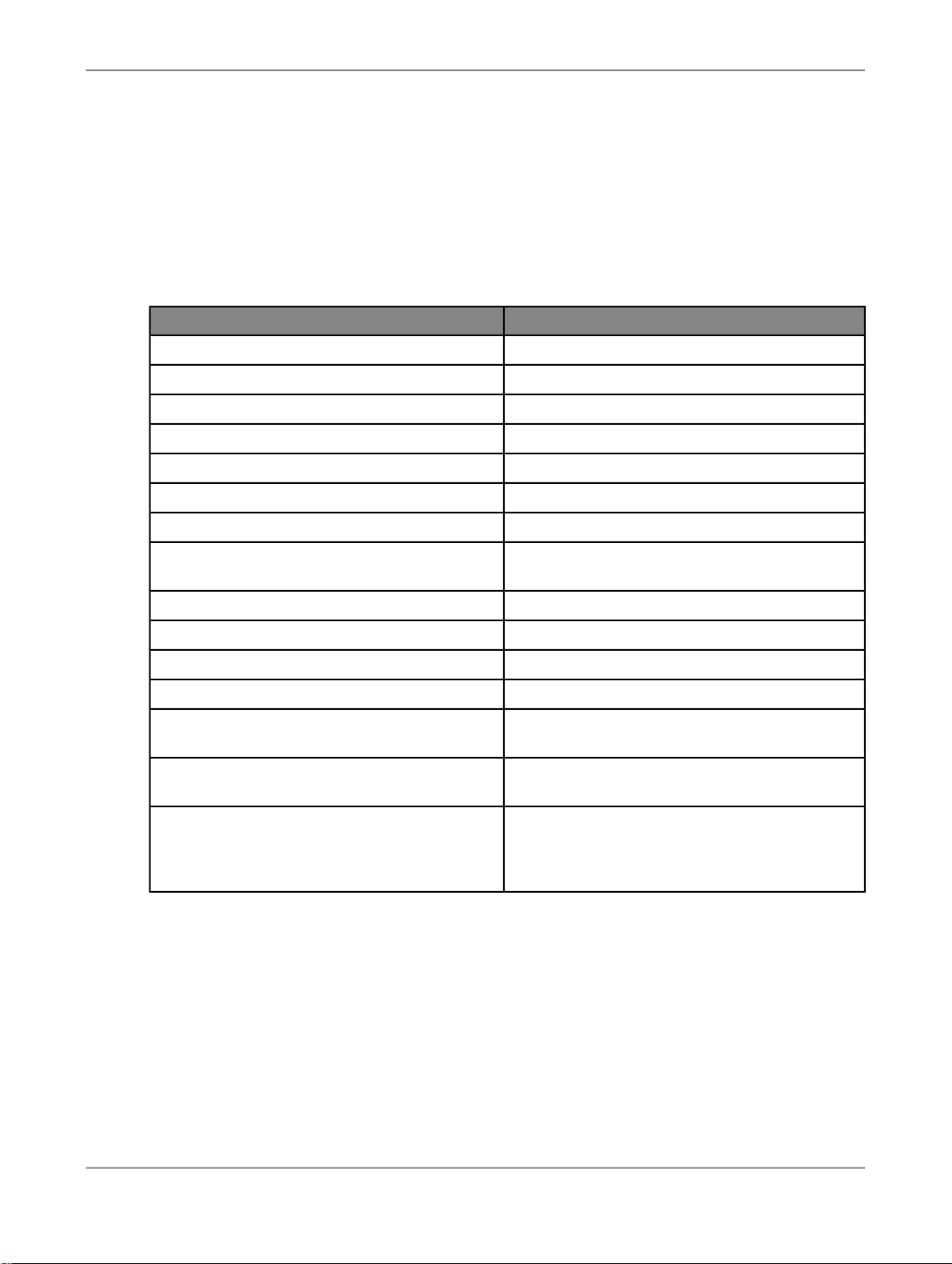
Creating Workbooks
4.6.4 Syntax for entering values
Follow these syntax rules when you enter members for filtering and values for prompting.
ExampleDescription
15Equal to
!22Exclude value
1-5Value range
!6-9Exclude value range
>8Greater than
!>8Exclude values greater than <value limit>
limit>
with A)*
exclude all values that begin with A)*
Dimension hierarchy node
>=8Greater than or equal to
!>=8Exclude values greater than or equal to <value
<12Less than
!<12Exclude values less than <value limit>
<=12Less than or equal to
!<=12Exclude values less than or equal to <value limit>
A*Contains pattern (for example, all values that begin
!A*Exclude values that contain pattern (for example,
<Dimension Attribute>(<Technical Name of Dimension>)
For example: ELEMENT1(WBS_ELEMENT)
2010-12-1248
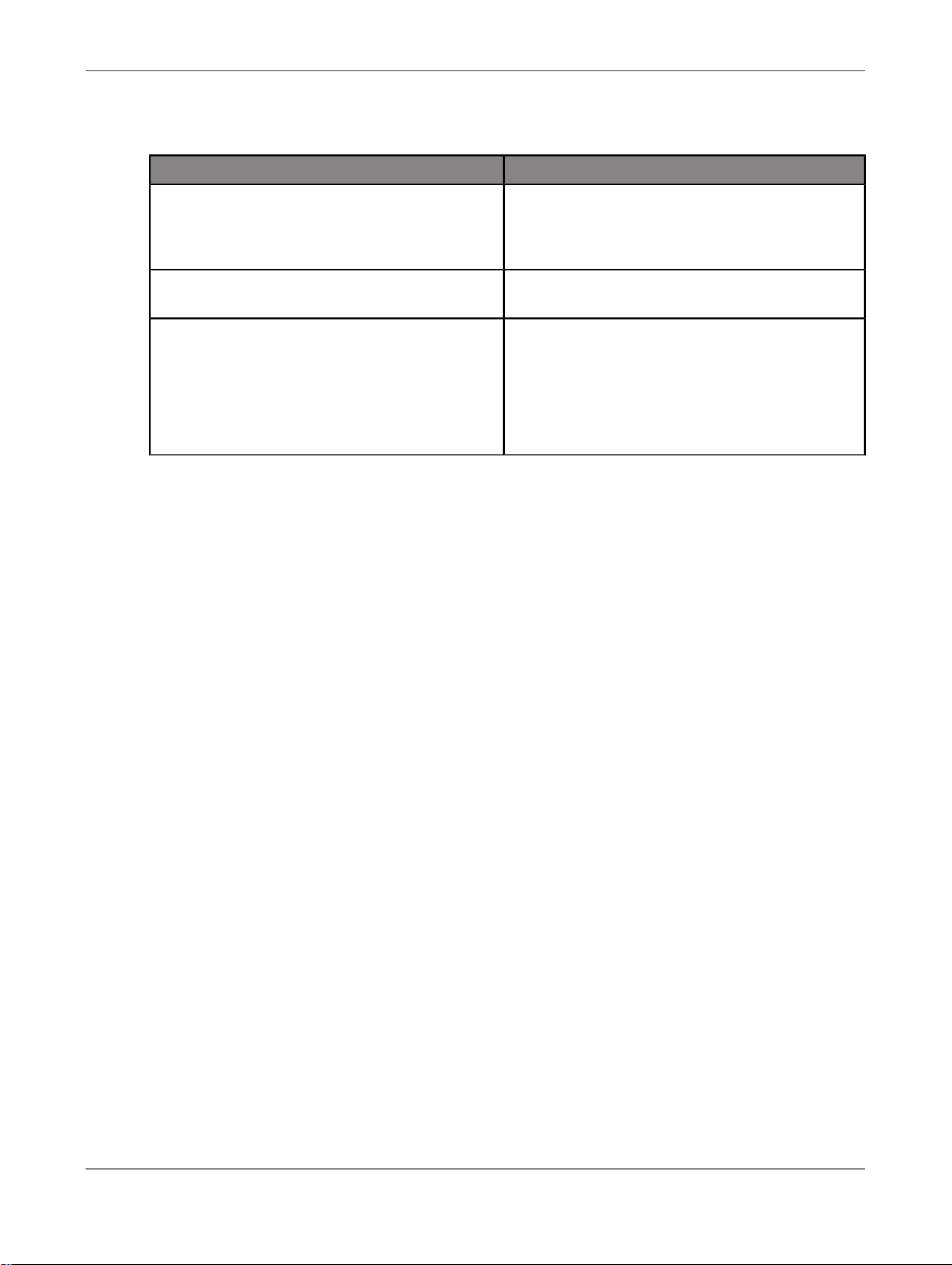
Creating Workbooks
ExampleDescription
Text hierarchy node
by a space
Escape character; backslash without space
*You can not use these syntax rules for filtering.
<Technical Name of Hierarchy Node>(0HIER_NODE)
For example: EUROPE(0HIER_NODE)
1-5; >12; !8Delimiter for multiple values; semicolon followed
\
If you enter a string that contains one of the special
characters used in these syntax rules, you can use
a backslash as escape character.
For example: Enter the string CA-QU as CA\-QU.
2010-12-1249

Creating Workbooks
2010-12-1250

Analyzing Data
Analyzing Data
5.1 To open a workbook
You can open a workbook that is stored on the SAP BusinessObjects Enterprise Server. This allows
you to see the navigation state that was saved with the workbook. You also get the workbook properites
that were saved with the workbook. These properties are part of the Component tab in the design
panel.
You can navigate through the data and design different views on the data. You can also add new data
sources or components.
1.
In Microsoft Excel 2007, press the Microsoft Office Button and choose Open Workbook.
In Microsoft Excel 2003, choose Open Workbook in the Advanced Analysis Standard toolbar.
2.
Enter your User, Password and the WEB Service URL to BusinessObjects Enterprise and press
OK.
3.
Select a workbook.
You can search for a workbook name or select a workbook in the BOE folder structure.
4.
Press OK.
The workbook is opened in Advanced Analysis.
5.
Choose Refresh All to refresh the data sources.
Note:
If the workbook property Refresh Workbook on Opening is selected on the Components tab in
the design panel, the refresh is executed automatically. In this case, you do not need to refresh the
data sources manually.
The selected workbook is opened in Advanced Analysis and you can start your analysis.
Related Topics
• Working with Advanced Analysis in Microsoft Excel 2007
• Working with Advanced Analysis in Microsoft Excel 2003
• The Components tab
2010-12-1251

Analyzing Data
5.2 Analyzing data with the design panel
The Advanced Analysis design panel is an additional element on the user interface that you can use
to create new views on your data, to find information on the used data sources and on the components
of the workbook. The design panel consists of three tabs: Analysis, Information and Components.
You can show and hide the design panel by choosing Display for the design panel.
You can choose Pause Refresh to deactivate the refresh after each navigation step. With the deactivated
refresh, you can design a new view on your data with multiple navigation steps. All steps will be executed
at once when you choose Pause Refresh again to activate the refresh. Note that most functions in the
menu are not available when Pause Refresh is activated. You should only work on the Analysis tab
when the automatic refresh is deactivated.
Related Topics
• The Analysis tab
• The Information tab
• The Components tab
5.2.1 The Analysis tab
On the Analysis tab, you can see the available fields for a single data source and the fields currently
used to display the data in a crosstab in columns and rows. If you use multiple data sources in your
analysis, select a crosstab cell of the required data source to specify which data source information
should be displayed.
The Analysis tab contains four sections:
• <Data source>
The heading for this section is the name of the selected data source. You can check wether you
have selected the right data source. The section displays all fields of the data source: measures,
dimensions, attributes and hierarchies.
• Columns
This sections contains all fields that are currently displayed in columns.
• Rows
This sections contains all fields that are currently displayed in rows.
• Background Filter
This sections contains all fields that are currently defined as background filters.
2010-12-1252

Analyzing Data
Navigating through the data
Using the Analysis tab, you have the following options to analyze data and create new views on it:
• You can use the context menu to move fields in the four sections. You can add a new dimension
from the <Data source> section to the Rows, for example.
• You can use drag and drop to move fields in the four sections.
• You can use drag and drop to add rows and columns to the crosstab. Drag a field directly to the
crosstab and drop it. The field is added automatically to the corresponding section on the Analysis
tab.
• You can also use drag and drop to remove a field from the crosstab. Select the border of a cell in
the crosstab to drag the field to the Analysis tab and drop it there.
• You can use the context menu to create, change and remove filters. If a filter is defined for an object,
you see a filter icon beside this object.
5.2.2 The Information tab
On the Infomation tab, you can see detailed information about a data source or the complete workbook.
You can also find information on filters and variables on this tab. The general information is displayed
as text elements.
In the Information for list, you can select the complete workbook or one of the inserted data sources.
The information fields are displayed for the selected object. You can insert these fields in the analysis
using drag and drop.
For a workbook, the following information is displayed:
• Workbook Name
• Created By
• Variables
• Logged On User
• Last Refreshed At
• Created At
• Last Changed At
For a data source, the following information is displayed:
• Data Source Name
• Key Date
• Last Data Update
• Filter
• Query Technical Name
• InfoProvider Technical Name
• InfoProvider Name
• Created By
• Last Changed By
• Last Changed At
2010-12-1253

Analyzing Data
• System
Related Topics
• To insert an info field
• To insert a filter
5.2.3 The Components tab
On the Components tab, you can see a list of all components used in the workbook together with the
properties of these components. You can select if the components should be listed by data source or
by sheet. In both cases, the highest node of the list is the workbook. Below this, the data sources or
the sheets are displayed with their components.
You can use the context menu to copy or delete a component or to move it to another sheet of the
workbook. On a data source, you can create a new table with the context menu. On a filter, you can
locate the filter in the analysis.
The following components and properties are displayed:
Name
Refresh Workbook on Opening*
Workbook
Force Prompt for Initial Refresh*
Store Prompts with Workbook*
DescriptionPropertiesComponent
Displays the name of the workbook.
The workbook name is defined when
saving the workbook.
If you select this check box, the data
sources in the workbook are refreshed
every time the workbook is opened.
If this check box is not selected, the
data in the workbook is not automatically refreshed on opening. You can refresh the data sources manually with
choosing Refresh All in the menu.
If you select this check box, the
prompting dialog is displayed on every
refresh.
If you select this check box, the defined
prompt values are saved with the
workbook
2010-12-1254
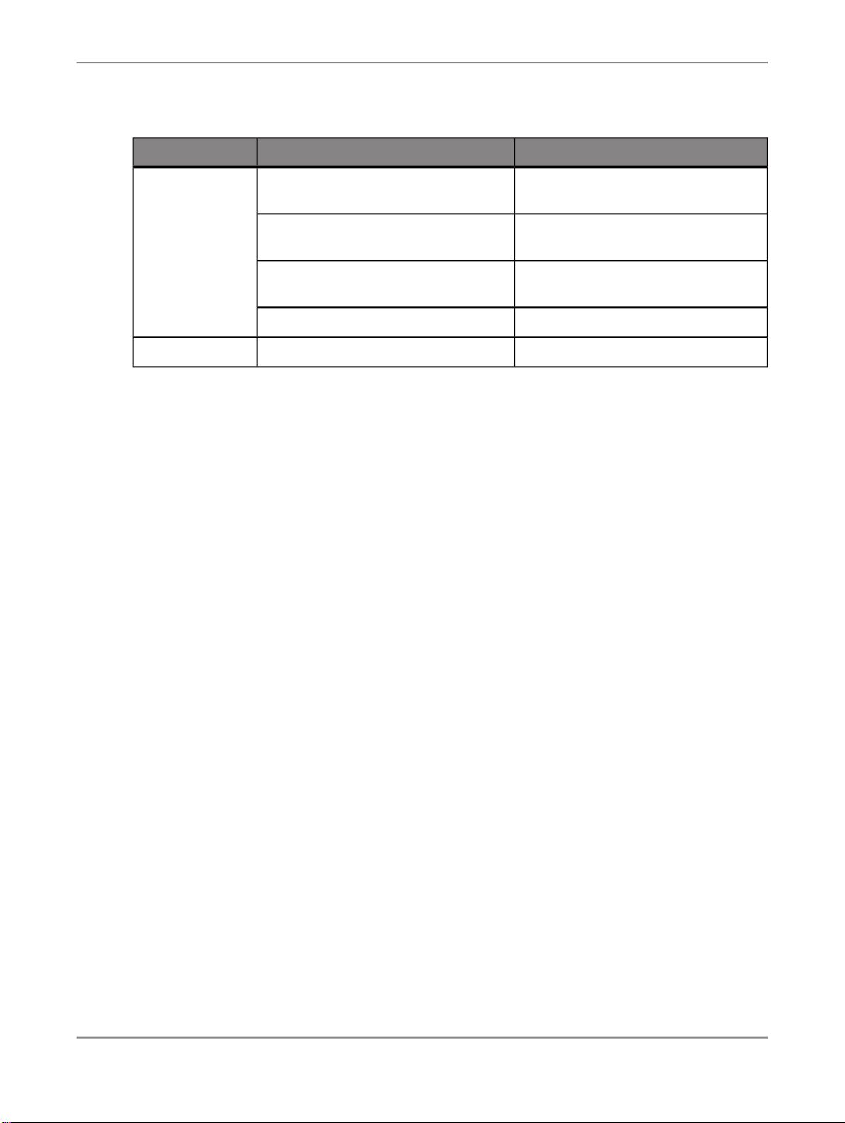
Analyzing Data
DescriptionPropertiesComponent
Data source
Data Source Name
Data Source Technical Name
Formula Alias
Displays the data source name. You
can change it here.
Displays the technical name of the data
source.
Displays the formula alias. You can
change it here.
Displays the system alias.System Alias
Displays the sheet name.NameSheet
2010-12-1255
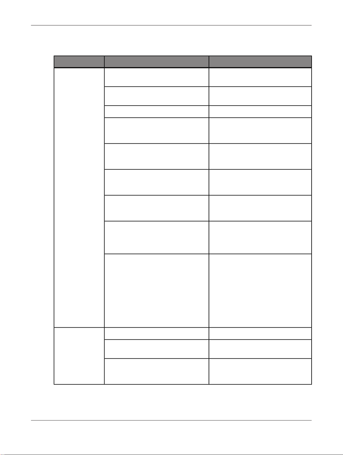
Analyzing Data
DescriptionPropertiesComponent
Crosstab
Name
Formula Alias
Range
Apply Default Formats
Display Symbols for Parent Members
Optimum Cell Width/Height
Repeat Members
Displays the crosstab name. You can
change it here.
Displays the formula alias. You can
change it here.
Displays the data source name.Data Source Name
Displays the cell range of the crosstab
in the sheet. You can change the range
to move the crosstab in the sheet.
If you select this check box, the default
formats are applied after each navigation step.
If you select this check box, a symbol
is displayed for parent members in a
hierarchy (+/-).
If you select this check box, the table
is displayed with optimum cell width
and height.
If you select this check box, texts that
are not displayed because they occur
several times in a column or row, are
repeated in each cell.
Filter
Wrap Headers
Dimension
Filter applies to the following data
sources
In BEx Query Designer, you can define
if key figures should be displayed in
multiple lines.
If you select this check box, these key
figures/measures are displayed in Advanced Analysis as defined in Query
Designer. If you clear the check box,
the measures are displayed in one
single line.
Displays data source name.Data Source Name
Displays the name of the filtered dimension.
You can select which of the available
data sources in the workbook should
be filtered.
2010-12-1256

Analyzing Data
DescriptionPropertiesComponent
Displays sheet and chart name.Name
Chart
* For more information on workbook properties, see To select workbook properties for prompting.
5.3 Prompting
In the prompting dialog, you can set values for prompts. Prompts are defined as variables in BEx Query
Designer. The variables are parameters of a BW query and are filled with values when you insert a
query as a data source in a worksheet. They serve as placeholders for members, hierarchies, hierarchy
nodes, formula elements and texts. After defining the variable values, the crosstab is displayed according
to the selected values.
To be editable in the prompting dialog, a variable must be defined as input-ready and set to Manual
Input in Query Designer. A variable can be defined as mandatory or optional in Query Designer.
If a query contains mandatory variables without default values, the prompting dialog appears automatically
when you insert the query in a worksheet and requires the definition of mandatory variable values before
the crosstab is added. If you cancel the prompting dialog, the query data is not included in the workbook.
Sheet
Displays the crosstab name.Cross Tab Name
Displays the sheet name. You can
change it here.
For queries with optional variables only, you can open the prompting dialog with the prompting icon in
the menu and define variable values. You can also use this manual option to open the dialog to change
existing values.
At workbook level, you can select properties to define how the prompting dialog and defined values
behave in workbooks. For example, you can define that variable values are saved in a workbook. If you
open this workbook again, the data is displayed according to the defined values. You can then open
the prompting dialog and change the values.
If there are no input-ready variables in the query that you use as your data source, the prompting dialog
is disabled.
Note:
Objects that are defined as input-ready variables in BEx Query Designer are called prompts in Advanced
Analysis, edition for Microsoft Office. In the following documentation the Advanced Analysis term prompt
is used for these variables. A query can also contain other variable types. All variables and values of
these variables that a query contains, are displayed in the Variables area on the Information tab in
the design panel.
2010-12-1257

Analyzing Data
To find more information about the definition of variables in the BEx Query Designer, go to the SAP
Help Portal at http://help.sap.comSAP NetWeaver > Select release and language > SAP NetWeaver
Library > SAP NetWeaver by Key Capability > Business Intelligence > BI Suite: Business Explorer
> Query Design: BEx Query Designer > Reusable Query components > Variables.
Related Topics
• To define prompt values
• To select workbook properties for prompting
5.3.1 To define prompt values
1.
Open the Prompts dialog.
In the Prompts Summary area, you see a list of all available prompts in the query and the selected
values. In the Specify Value for Prompts area, you can expand single prompts to define values.
The mandatory prompts are marked with an asterisk. If default values for the prompts are defined
in BEx Query Designer, they are displayed as selected in the prompting dialog.
2.
In the list box, select whether all prompts, no prompts or only the mandatory prompts are expanded
in the Specify Value for Prompts area:
• Select Collapse All if all prompts should be displayed collapsed.
• Select Expand All if all prompts should be displayed expanded.
• Select Show all mandatory prompts if only these prompts should be displayed expanded. This
is the default option.
3.
Define values for the expanded prompts.
You can define values for the following prompt types. Depending on the prompt definition in BEx
Query Designer, you have various options:
2010-12-1258

Analyzing Data
Value DefinitionPrompt Type
Dimension*
Dimension*
Dimension*
Dimension*
Single value
You can select one member as the prompt value for this dimension.
Multiple value
You can select multiple members as the prompt values for this dimension.
Press the + button, to add a field for additional values. Press the Filter button
if you want to select multiple values in a list at once. To remove a selected
member, press the red X button.
Value range
You can select a start and an end member to define a range of values for this
dimension.
Selection option
You can select an operator and corresponding members to define a selection
for this dimension. The following operators are available: Between, Outside,
Equal To, Not Equal to, Greater Than, Greater Than or Equal To, Less Than,
Less Than or Equal To.
You can add multiple selections for this dimension. Press the + button, to add
a selection. To remove a selection, press the red X button.
Hierarchy
Hierarchy node*
You can select a hierarchy from the list box to define a prompt value.
Single value
You can select one hierarchy node as the prompt value for the selected hierarchy.
2010-12-1259

Analyzing Data
Value DefinitionPrompt Type
Hierarchy node*
Multiple value
You can select multiple hierarchy nodes as the prompt values for the selected
hierarchy.
Press the + button, to add a field for additional value. Press the Filter button
if you want to select multiple values in a list at once. To remove a selected
member, press the red X button.
Formula
You can enter a numeric value.
The numeric value is used for measure calculations defined in BEx Query Designer with prompts.
Text
You can enter a text.
This prompt type can be used to assign text to columns or row headers or to
change the description of a calculated measure.
* For these prompt types, you can enter the values manually or using input help. When you open
input help, no values are selected. You can search for members or select members directly from
the list. You can also define if the members in the list should be displayed with key, text, or both.
For hierarchical dimensions, you can define if the members should be displayed in hierarchies, at
leaf level, or on a specific level.
4.
Press OK to apply the selected values to your data.
The system validates all prompt values. If the validation is successful, the crosstab is displayed
according to your selection.
The data in the worksheet is displayed according to your selection. You can see the selected values
in the Filter area on the Information tab in the design panel. The defined prompt values can be saved
with the workbook and are then available to other users or in other sessions. To change the prompt
values, open the prompting dialog again.
5.3.2 To select workbook properties for prompting
You can select various workbook properties in the design panel that affect the behavior of the prompting
dialog and existing prompt values:
1.
Open the Design Panel in the menu.
2.
Select the Components tab.
3.
Select the required workbook properties in the Properties area. The following properties are available:
• Refresh Workbook on Opening
2010-12-1260

Analyzing Data
If you select this option, the data sources in the workbook are refreshed every time the workbook
is opened. The behavior of the prompting dialog depends on the other properties you selected
for this workbook.
If this check box is not selected, the data in the workbook is not automatically refreshed on
opening. You can refresh the data sources manually with choosing Refresh All in the menu.
• Force Prompt for Initial Refresh
If you select this option, the prompting dialog is displayed on every refresh. The dialog appears,
even if the query contains only optional prompts. If values are already saved with the workbook,
these are displayed as predefined settings in the dialog. You can accept or change these values.
A refresh happens when you open a workbook and select refresh, when you select the setting
above and open a workbook or when you insert a new data source.
If this property is not selected, the system checks whether the workbook contains mandatory
variables that no values are available for. If no values are available, the prompting dialog is
displayed; if values are available, the workbook is displayed straight away.
• Store Prompts with Workbook
This is the default property. If it is used, the defined prompt values are saved with the workbook
and will be applied to the data when the workbook is refreshed during the current session or
closed and opened again. The prompt values are also available to other users using the workbook.
To change the values, you can open the prompting dialog manually.
If this property is not selected, the defined values will not be saved with the workbook.
The behavior of the prompting dialog and saved prompt values will work according to your workbook
properties selection.
5.4 Filtering data
In Advanced Analysis, you can define criteria to restrict the data displayed in your analysis to a subset
of data. This action is called filtering. With filtering, you define which subset of data appears in the
analysis. This allows you to create new, more specific views of your data. Filters are additive, which
means that each additional filter is based on the current filter and further reduces the subset of data.
There are two types of filters. With "Filtering members", you can specify which members to display and
which not to display in your analysis. You can also define members to use as filters in the background
of the anlysis. With "Filtering measures", you can specify which measure values should be displayed
in the analysis. For example, you can define that you want to see the Top 3 regions in sales volume
for each product in your analysis. You can also filter out rows and columns that contain only zeros.
Related Topics
• Filtering members
• Filtering measures
• To show/hide zeros in rows and columns
2010-12-1261

Analyzing Data
5.4.1 Filtering members
By selecting and removing members of your analysis, you can create new views of your data. You can
filter members of a flat dimension with the filter dialog or directly on the crosstab. You can also filter
members of a hierarchical dimension (hierarchy). The measures in an analysis are combined to one
dimension, the measure dimension. You can also define criteria that are used in the background of the
analysis for filtering.
For example, if you analyse the sales volume of your company in the last three years, and you only
want to see the values for the last three month of each year, you can remove the other months from
your analysis.
Filtering members is a static action. Members that you have removed from your analysis remain excluded
unless you change the filter criteria and include them again.
Member filters affect the totals and subtotals in your analysis. Only the values for the displayed members
are included in the totals.
Related Topics
• To filter data by member
• To filter data by member within hierarchies
• To filter members directly on the crosstab
• To filter out members directly on the crosstab
• To create a background filter
• To remove a filter by member
5.4.1.1 To filter data by member
1.
Select a cell in the crosstab that belongs to the dimension you want to use for filtering.
2.
Choose Filter > Filter by member.
The "Filter by Member" dialog box appears.
Note:
You can also open this dialog box using the context menu on the crosstab or the design panel.
3.
Select Individual Selection if you want to filter individual members of the dimension.
a. If you want to search for members, clear the Select All check box in the members list and enter
a search string in the entry field. In the drop-down list of the search button, you can select if you
want to search for a key or text.
Members that match the search string are displayed in the members list and can be selected.
2010-12-1262

Analyzing Data
4.
b. With the Display list, you can select how the members are displayed in the list. The following
options are available: Key, Text, Text and key, Key and text.
c. Press the Show Selected button if only the selected members should be displayed.
The button name changes to Show All. Press this, if you want all members to be displayed again.
d. Select the members that you want to use for filtering in the members list.
In the members list, all members are selected in the default setting. To deselect a member, clear
the corresponding check box. You can also deselect all members by clearing the Select All
check box and selecting individual members from the list.
Select Range Selection if you want to filter for a range of members.
a. Select an operator.
The following operator are available: Between, Outside, Greater Than, Greater Than Or Equal
To, Less Than, Less Than Or Equal To, Equal To and Not Equal To.
b. Select the member range.
For the range definition, the key of the members is relevant, not the text.
c. Select Add Range.
The range is added to the "Range" area. You can add several ranges to the filter.
5.
Press OK to apply the filter to your data.
The data in the worksheet is filtered according to your selection. The filter is saved with the workbook
and is available to other users or in other sessions. You can also open and edit existing filters again.
5.4.1.2 To filter data by member within hierarchies
The data source you use, includes hierarchies.
1.
Select a cell in the crosstab that belongs to the hierarchy you want to use for filtering.
2.
Choose Filter > Filter by member.
The "Filter by Member" dialog box for hierarchies appears.
Note:
You can also open this dialog box using the context menu on the crosstab or the design panel.
3.
If you want to search for members, clear the Select All check box in the members list and enter a
search string in the entry field. In the drop-down list of the search button, you can select if you want
to search for a key or a text.
Members that match the search string are displayed in the members list and can be selected.
4.
With the Display list, you can select how the members are displayed. The following options are
available: Key, Text, Text and key, Key and text and Show Attributes.
In the Show Attributes list, you can find the attributes that are available for the members in your
hierarchy. For example, a product hierarchy could have size and colour as attributes. You can select
2010-12-1263

Analyzing Data
5.
6.
7.
8.
and add these attributes to the member list in the filter dialog. This additional information may help
you to make the selections for filtering.
Select in the list box which members should be displayed in the list for selection.
• Select Hierarchy in the list if you want the members to be listed with the hierarchy.
• Select Leaves if you want all members of all levels to be listed in a flat view.
Press the Show Selected button if only the selected members should be displayed.
The button name changes to Show All. Press this if you want all members to be displayed.
Select the members that you want to use for filtering in the members list.
In the members list, all members are selected in the default setting. To deselect a member, clear
the corresponding check box. You can also deselect all members by clearing the Select All check
box and selecting individual members from the list.
If you deselct a node in a hierarchy, all leaf members of this node are deselcted automatically. The
parent members of the deselcted node are still selected, but the background color of the check box
changes to gray. That shows you that not all leaf members of this node are selected for filtering.
Press OK to apply the filter to your data.
The data in the worksheet is filtered according to your selection. The filter is saved with the workbook
and is available to other users or in other sessions. You can also open and edit existing filters again.
5.4.1.3 To filter members directly on the crosstab
You can filter for one or multiple members directly using the context menu.
1.
In the crosstab, select one cell for each member that you want to filter for.
To select multiple members, hold down the Ctrl or Shift key as you select members.
2.
Choose Filter Members in the context menu.
In the design panel, the filter icon is added to the corresponding dimension.
The data in the worksheet is filtered according to your selection. You can apply this filtering to dimensions
with and without hierarchies.
5.4.1.4 To filter out members directly on the crosstab
You can filter out one or multiple members directly using the context menu or drag and drop.
1.
In the crosstab, select one cell for each member that you want to filter out.
To select multiple members, hold down the Ctrl or Shift key as you select members.
2.
Choose Filter Other Members in the context menu.
2010-12-1264

Analyzing Data
To filter out the selected members using drag and drop, select the border of the marked field(s) and
drag them out of the crosstab.
In the design panel, the filter icon is added to the corresponding dimension.
The data in the worksheet is filtered according to your selection. You can apply this filtering to dimensions
with and without hierarchies.
5.4.1.5 To create a background filter
In Advanced Analysis, you can set filters for dimensions and hierarchies that you have chosen to be
displayed in the crosstab. This allows you to narrow the scope of your analysis to the data you need.
You can however also select members for filtering that should not be displayed in the crosstab. These
non-visible filters are background filters.
For example, you have selected the dimensions Product and Region to be displayed in the crosstab.
The data source contains the sales volume for the years, 2008, 2009 and 2010. If you are only interested
in the sales volume for 2010, you can add the Year dimension as a background filter to your analysis
and filter for 2010. The analysis will show the data for year 2010, but the Year dimension is not visible
in the crosstab.
Note:
Background filters for a measure dimension can contain only one measure as a filter. The same is true
for other dimensions that do not aggregate.
You have the following options to add a background filter to your analysis:
1.
You can add a dimension to the Background Filter area and define a filter:
a. Add the dimension that you want to add to the Background Filter area in the design panel.
You can add the dimension using drag and drop or you can choose Move to Background Filter
in the context menu.
b. Choose Filter By Member in the context menu.
The "Filter by Member" dialog box appears.
c. Make your selection and press OK.
The background filter is created.
2.
Or: You can add a dimension that already has a filter. The existing filter will be applied as a
background filter in the crosstab.
3.
Or: You can add a background filter using the context menu on the crosstab.
a. Select the member(s) that you want to define as background filter in the crosstab.
b. Choose Filter Members and Swap With in the context menu.
The dimension with the selected filters is added automatically to the Background Filter area,
and the dimension chosen for swapping with is added to the Rows area in the design panel.
The data in the crosstab is displayed according to your filter selection.
2010-12-1265

Analyzing Data
5.4.1.6 To remove a filter by member
1.
Select a cell in the crosstab that belongs to the dimension you want to remove the filter for.
2.
Choose Filter > Select All Members.
Note:
You can also choose Select All Members in the context menu on the crosstab or the design panel.
All members of the selected dimension are displayed in the crosstab.
5.4.2 Filtering measures
With filtering measures, you can define rules to filter the data of your analysis to your current scope of
interest. You can apply one or multiple rules to a measure. Depending on where you open the Filter
by measure dialog, the filter definition is applied to a selected dimension, to all dimensions or to the
most detailed dimension in your analysis. The applied measure filters do not affect totals or subtotals
in your analysis.
You can define rules to get a ranked list of data and a list of data matching a threshold value.
In a ranked list filtering, all entries of the currently displayed data are considered and their relationship
to each other determines whether an entry is displayed. For example, you can define that the Top 3
entries for a measure should be displayed.
In a threshold list filtering, an entry is filtered independently of the other entries if its value matches the
criteria in the defined rule. For example, you can define that all entries are displayed that are greater
than a specific threshold value.
Filtering measures is a dynamic action. Whenever you change the view of your data, the filter is applied
again. For example, if you add a Top 5 filter, five members are shown in your analysis. If you then add
members that you previously removed from the analysis, some of these newly added members could
match the Top 5 criteria and replace some of the previously displayed members.
Related Topics
• To filter data by measure
• To remove a filter by measure
2010-12-1266

Analyzing Data
5.4.2.1 To filter data by measure
1.
You have the following options to open the filter dialog:
• Select a cell belonging to a dimension in the crosstab and choose Filter > Filter by Measure >
Edit.
If you select this option, the filter is applied to the members of the selected dimension.
• Select a cell belonging to a measure in the crosstab and choose Filter > Filter by Measure >
All Dimensions Independantly > Edit.
If you select this option, the filter is applied to all dimensions in the analysis, from the outermost
to the most detailed one. For example, in an analysis with three dimensions in columns A, B and
C, the filter is first applied to the dimension in column A, then to the dimension in column B and
finally to the dimension in column C.
• Select a cell belonging to a measure in the crosstab and choose Filter > Filter by Measure >
Most Detailed Dimension in Rows > Edit.
If you select this option, the filter is applied to the most detailed dimension of the rows. For
example, in an analysis with three dimensions in columns A, B and C, the filter is applied to the
dimension in column C. This option is optimized for threshold value filtering.
• Select a cell belonging to a measure in the crosstab and choose Filter > Filter by Measure >
Most Detailed Dimension in Columns > Edit.
If you select this option, the filter is applied to the most detailed dimension of the columns. For
example, in an analysis with three dimensions in rows 2, 3and 4, the filter is applied to the
dimension in row 4. As with the option above, this option is also recommended for threshold
value filtering.
The "Filter by Measure" dialog box appears.
Note:
You can also open this dialog box using the context menu on the crosstab or the design panel.
2.
In the Based on measure: list, select the measure you want to use.
3.
In the Definition area, select the operator and value for a new rule.
The following operators are available: Between, Outside, Greater Than, Greater Than or Equal to,
Less Than, Less Than or Equal to, Equal to, Top N, Bottom N, Top%, Bottom %, Top Sum, Bottom
Sum.
4.
Press Add.
The new rule is added to the Rules area.
5.
If you define multiple rules, select the logic for the rules.
Select AND, if all rules should be applied simultaneously, or OR , if only one of the rules should be
applied.
6.
Press OK.
2010-12-1267

Analyzing Data
The data in the worksheet is filtered according to your selection. The filter is saved with the workbook
and is available to other users or in other sessions. You can also open and edit existing filters again.
5.4.2.2 Operators used for filtering measures
When defining filters by measure, you can create rules to get a list of data for a defined threshold value
and rules to get ranked list of data.
To define threshold values, you can use the following operators:
• Between / Outside
For these operators, you define a range of values that should be included or excluded in the list.
• Greater Than / Less Than
For these operators, you define a specific value to display members that are greater or less than
this value.
• Greater Than or Equal to / Less Than or Equal to
For these operators, you define a specific value to display members that are greater or equal to or
less or equal to this value.
• Equal to
For this operator, you define a specific value to display members that are equal to this value.
To define a ranked list of values, you can use the following operators:
• Top N / Bottom N
For these operators, you must enter a whole, positive number as the value. The ranked list is arranged
according to the defined number.
For example, if you want a list of the three customers with the strongest sales volume and the five
customers with with the weakest sales volume, you create a Top 3 and a Bottom 5 rule in the filter
definition.
• Top% / Bottom %
For these operators, you must enter a number between 0 and 100. The ranked list is arranged
according to the defined percentage.
For example, if you want a list of the strongest products in revenue until 25% of the total revenue is
attained, you create a Top 25% rule for this measure with regard to products.
• Top Sum / Bottom Sum
For these operators, you can also enter a floating point number (15.7 for example). The ranked list
is arranged according to the defined total value.
2010-12-1268

Analyzing Data
For example, you want a list of products with the highest sales volume, whose combined sales
volume totals EUR 20,000. All sales volumes are first sorted in descending order. The totals are
calculated until the threshold value of 20,000 is exceeded. If the last value that need to be included
to achieve EUR 20,000, causes the total to exceed 20,000, it is also included in the list. All products
with a lower sales volume than this product are no longer displayed. Products that exceed the EUR
20,000 threshold remain in the list.
Note:
Do not use these operators for ranked lists for filtering hiearchies.
5.4.2.3 To remove a filter by measure
1.
Select a cell in the crosstab.
There are four options for defining a filter by measure. To delete an existing filter, you have to select
a cell that belongs to the option you used for defining the filter.
2.
Choose Filter > Filter by measure > [Selected Filter Option] > Reset.
Note:
You can also use the context menu on the crosstab.
The data in the crosstab is displayed without the removed filter.
5.4.3 To show/hide zeros in rows and columns
1.
Select a cell in the crosstab.
2.
Choose Filter and one of the following options:
• Suppress Zeros in Rows
All rows that only contain zeros are removed.
• Suppress Zeros in Columns
All columns that only contain zeros are removed.
The zeros are suppressed in rows and/or columns. When zero suppression is active, a check mark is
displayed beside the menu item.
To restore the hidden rows and columns, choose Filter > Suppress Zeros in Rows or Filter > Suppress
Zeros in Columns again.
You can also define how zeros should be displayed in the crosstab if they are not hidden.
2010-12-1269

Analyzing Data
Related Topics
• To define the display of zeros and negative values
5.5 Sorting data
Sorting data is a fundamental part of data analysis. It helps you understand your data better as you can
visualize and organize different views on the data in your crosstab. With sorting the data, you are able
to quickly identify the data you need for your decisions.
You can sort data by values (smallest to largest and largest to smallest) and members (A to Z and Z
to A). If you sort the values of one measure (for example sales volume) from smallest to largest, the
other cells in your crosstab are also affected by the sorting. The metadata information therefore remains
correct in the crosstab.
The following sorting options are available:
• Ascending
If you select ascending sorting, the data is sorted from smallest to largest. Ascending sorting for
members results in sorting from A to Z.
• Descending
If you select descending sorting, the data is sorted from largest to smallest. Descending sorting for
members results in sorting from Z to A.
• Break Hierarchies
In the default setting, data is sorted in the hierarchy levels of the crosstab. Parent members are
sorted in order, and child members are sorted below each parent member in their own order. If you
want to sort data across the entire hierarchy, select the "Break Hierarchies" option.
Related Topics
• To sort values
• To sort members
5.5.1 To sort values
1.
Select a cell in the crosstab that belongs to the measure you want to use for sorting.
2.
Choose Sort > More Sort Options....
The "Sort by" dialog box appears.
2010-12-1270

Analyzing Data
3.
4.
The sorting is applied to the crosstab.
Select the sort options you want to use:
• Sort Ascending
Sorts values from smallest to largest.
• Sort Descending
Sorts values from largest to smallest.
• Break Hierarchies
If you select this option, the values are sorted across hierarchies. Existing hierarchies in the
crosstab and their subtotals are not available any more after sorting. In the default setting, the
option is not selected.
Note:
If you do not want to change the settings for Break Hierarchies, you can also select the sorting
options Sort Ascending and Sort Descending directly in the menu or context menu.
Press OK.
5.5.2 To sort members
1.
Select a cell in the crosstab that belongs to the dimension you want to use for sorting.
2.
Choose Sort > More Sort Options....
The "Sort by" dialog box appears.
3.
Select the sort option you want to use:
• Sort Ascending
Sorts members from A to Z.
• Sort Descending
Sorts members from Z to A.
4.
In the Sort by list, select the object type for sorting:
• Default (Dimension Members by First Display Type)
The members are sorted by the first display type of the selected dimension.
• Member Display Type
You can select one of the member display types in the list below.
• Measure
If you select this object type, you can select one of the available measures in the list below. With
this object type, the sorting is applied to the values of the selected measure and not to a dimension.
2010-12-1271

Analyzing Data
Note:
If you do not want to change these settings, you can also select the sorting options Sort Ascending
and Sort Descending directly in the menu or context menu.
5.
Select Break Hierarchies if you want to sort the members across hierarchies. Existing hierarchies
in the crosstab and their subtotals are not available any more after sorting.
6.
Press OK.
The sorting is applied to the crosstab.
5.6 Working with hierarchies
There are two option to work with hierarchical presentations in your analysis: Dimensions with hierarchies
and Dimensions displayed as hierarchy.
Including dimensions with hierarchies
Hierarchies for dimensions are created in the data modeling of SAP NetWeaver BW. In SAP NetWeaver
BW, they are called "Characteristic Hierarchy". A dimension can contain multiple hierarchies. In a
hierarchy, dimension members are organized in a tree structure. For example, the hierarchy of cost
centers that are assembled in cost center groups.
Note that dimension with hierarchies can behave differently during filtering and sorting. The behavior
is described in the corresponding chapters.
To find more information about the definition of characteristic hierarchies in SAP NetWeaver BW, go
to the SAP Help Portal at http://help.sap.comSAP NetWeaver > Select release and language > SAP
NetWeaver Library > SAP NetWeaver by Key Capability > Business Intelligence > BI Platform >
OLAP > Hierarchies.
Displaying single dimensions as hierarchy
You can display multiple dimensions in a crosstab as flat presentation or as hierarchy. By default, the
flat presentation is displayed. You can change the display to a hierarchical presentation. You can also
use dimensions with hierarchies as a single dimension and combine it with other dimensions to a
hierarchical presentation.
Related Topics
• To include dimensions with hierarchies in an analysis
• To display single dimensions as hierarchy
• To filter data by member within hierarchies
• Sorting data
2010-12-1272

Analyzing Data
5.6.1 To include dimensions with hierarchies in an analysis
By using a data source that contains a dimension with hierarchies, you can define different views on
the hierarchies of the dimension. You can also display the members of the dimension in a flat
presentation.
As of step two, the steps in the following procedure are optional. You can use the options you need to
define your view on the data.
1.
Move a dimension with hierarchies to the "Rows" section in the design panel.
Note:
Dimensions can also be moved to the Columns section. This procedure describes dimensions in
the Rows section. Dimensions in columns behave accordingly.
The dimension is displayed in the crosstab. If the dimension contains more than one hierarchy, the
displayed hierarchy is selected according to the definition in the BEx Query Designer. Nodes with
a + contain subnodes.
2.
Select a different hierarchy.
Select a different hierarchy of the dimension in the <data source> section in the design panel and
move it to the dimension in the Rows section.
The data in the crosstab changes according to your selection.
3.
Expand/Collapse all nodes.
Select the cell with the dimension name in the crosstab and choose Hierarchy > Expand to Level
> <Level>. The number of available levels depends from the hierarchy.
The levels in the crosstab are expanded according to your selection. To collapse the levels, choose
the first level.
4.
Expland/Collapse a single node.
Select a node cell in the crosstab that you want to expand and choose Hierarchy > Expand .
The selected node is expanded to the next level. To collapse the subnodes of a selected node,
choose Hierarchy > Collapse. You can also select the +/- symbols to expand and collapse a single
node.
5.
Define the available levels of the hierarchy.
Select a member cell of the dimension in the crosstab and choose Hierarchy > Show Level....
Select the levels that should be available in the analysis and press OK.
Only the selected levels can be displayed in the crosstab. The total is not affected by this selection
because the leaf level is always available.
6.
Define the sequence of a hierarchy.
By default, a hierarchy is displayed from parent level to child level. To change this presentation,
select the node of the first level and choose Hierarchy > Expand Upwards (Rows).
The hierarchy is displayed from child level to parent level.
7.
Display the dimension as flat presentation.
2010-12-1273

Analyzing Data
Select the Flat Presentation node in the <data source> section of the design panel and move it to
the dimension in the Rows section.
The members of the dimensions are displayed in a flat presentation.
The dimension with hierarchies is displayed according to your definition.
5.6.2 To display single dimensions as hierarchy
If you use multiple dimensions in your analysis, you can display them as flat presentation or as hierarchy
in the crosstab.
As of step three, the steps in the following procedure are optional. You can use the options you need
the define your view on the data.
1.
Move at least two dimensions to the "Rows" section in the design panel.
Note:
Dimensions can also be moved to the Columns section. This procedure describes dimension in the
Rows section. Dimensions in columns behave accordingly.
The dimensions are displayed side by side in the crosstab.
2.
Change to hierarchical display.
Select a crosstab cell and choose Hierarchy > Compact Display in Rows.
The dimensions in the crosstab are displayed as hierarchy. The first dimension in the Rows section
is the first level in the hierarchy. Nodes with a + contain subnodes.
3.
Expand/Collapse all nodes.
Select the cell with the dimension name in the crosstab and choose Hierarchy > Expand to
Dimension > <Dimension Name>. The number of available dimensions depends from the number
of dimensions in the Rows section.
The hierarchy in the crosstab is expanded according to your selection. To collapse the hierarchy,
choose the first dimension.
4.
Expand/Collapse a single node.
Select a node cell in the crosstab that you want to expand and choose Hierarchy > Expand
Dimension <Dimension Name>.
The selected node is expanded to the next dimension below. To collapse the subnodes of a selected
node, choose Hierarchy > Collapse. You can also select the +/- symbols to expand and collapse
a single node.
5.
Define the sequence of the dimensions in the hierarchy.
The sequence of the dimension in the Rows section determines their level in the hierarchy. The first
dimension in the design panel is the first level in the hierarchy. By using drag and drop, you can
move the dimensions up and down. The levels in the hierarchy are changed immediately.
The hierarchy is displayed from child level to parent level.
6.
Display the dimensions again as flat presentation.
2010-12-1274

Analyzing Data
Select a crosstab cell and choose Hierarchy > Compact Display in Rows.
The dimensions are again displayed side by side in the crosstab.
The dimensions are displayed according to your definition.
5.7 Calculating new measures
Based on measures that are available in your analysis, you can calculate new measures. There are
two types of calculations.
For simple calculations, you use two or more available measures as operands and an operator to create
a new measure. The new measure is the sum of two available measures, for example.
For dynamic calculations, you only use one available measure as operand and you create a new
measure based on this operand. For example, if you use sales volume per region as operand, you can
add a new measure that displays the rank of each region according to sales volume. If you now filter
out or add new regions to your analysis, the rank numbers are changed dynamically. These calculations
are therefore called dynamic calculations.
The newly created measures are added to the crosstab and to the design panel. In the design panel,
you can switch the sequence of the measures, edit their name or delete them. Directly on the crosstab,
you can also switch the sequence using drag and drop, and edit the name and delete measures with
the context menus.
Related Topics
• To calculate a new measure based on available measures
• To add a new measure based on one available measure
5.7.1 To calculate a new measure based on available measures
1.
Select the measure headings that you want to use.
The first measure that you select is the first operand. Use the STRG key to select the next measure
that is the second operand. You can also select more than two operands for your calculation.
2.
Choose Calculations > Add Calculation > [Operator].
The following operators are available:
• Add
• Substract
• Multiply
• Divide
• Percentage Difference
2010-12-1275

Analyzing Data
The new calculated measure is added to the crosstab and the design panel.
The new measure calculates the difference between operand 1and operand 2 as a percentage.
For example, operand 1 has value 80 and operand 2 has value 20. The new measure displays
the value 300%, as the difference is 60 and 60 is 300% of 20.
If operand 2 has a higher value than operand 1, the result is negative. For example, operand 1
has value 20 and operand 2 has value 80. The new measure displays the value -75%, as the
difference is -60 and -60 is -75% of 80.
• Percentage Share
The new measure calculates the share of operand 1 in comparison with operand 2 in percentage.
For example, operand 1 has value 20 and operand 2 has value 80. The new measure displays
the value 25%, as 20 is 25% of 80.
5.7.2 To add a new measure based on one available measure
1.
Select the measure heading that you want to use.
2.
Choose Calculations > Add Dynamic Calculation > [Operator].
The following operators are available:
DescriptionOption
Moving Minimum Value
Moving Maximum Value
Accumulative Sum
The new measure displays the smallest value available up to this point.
For example, there are ten rows with values in your
crosstab. The new measure starts in the first row
with the same value as the original measure. If the
second row in the original measure has a higher
value than the first, the value of the first row is repeated in the second row of the new measure and so on.
The new measure displays the highest value available up to this point.
The new measure displays the sum of all values up
to this point.
For example, the original measure has eight rows
with values. In the fourth row of the new measure,
the sum of first four rows is displayed.
Accumulative Sum of Rounded Values
The new measure displays the sum of all rounded
values up to this point.
2010-12-1276

Analyzing Data
DescriptionOption
Accumulative Count of All Detailed Values
Accumulative Count of All Detailed Values
that are Not Zero, Null or Error
Moving Average
Moving Average that is Not Zero, Null or
Error
Rank Number
The values per measure are counted and numbered
starting with 1 for the first value. If there are 8 rows
with values, including zeros, that contribute to the
total, the new measure displays the numbers 1 to 8
for the 8 values.
The values per measure are counted and numbered
starting with 1 for the first value, excluding values
that are equal to zero.
For values that are equal to zero, the last number is
repeated.
The new measure calculates the average of all values
up to this point.
For example, if there are five rows with values in the
crosstab, the new measure calulates in row 2 the
average of the values in row one and two, and so
on.
The new measure calculates the average of all values
up to this point, excluding values that are equal to
zero.
The new measure displays a rank number for each
value of the original measure. The highest value in
the original measure has the rank number 1.
If a value occurs more than once, the values are assigned to the same rank number. If there are two
identical values with rank number 4, the next smallest
value has rank number 5.
Olympic Rank Number
The Olympic ranked list differs from the basic ranked
list as follows: In the Olympic ranked list, when a
value occurs more than once, the next smallest value
is not assigned the rank incremented by one, but the
rank that corresponds to the number of previous
values (including the current value).
For example, if the rank 4 occurs twice, the new
measure displays number 6 for the next smallest
value rank.
Percentage Contribution
The new measure calculates the percentage contribution of a value in the original measure to the
overall result of the original measure.
The new measure is added to the crosstab and the design panel.
2010-12-1277

Analyzing Data
5.8 Defining Conditional Formatting
You can use conditional formatting to highlight important values or unexpected results in your data.
With conditional formatting, you define rules to select different or critical values in a crosstab. Results
that fall outside a set of predetermined threshold values are highlighted in color or designated with
symbols. This enables you to identify immediately any results that deviate from the expected results.
For example, you directly see answers to questions, such as which products have over 10% revenue
increase this year or which regions have sales volume higher than a defined amount.
You can add one or more rules to a conditional format and prioritize the application of the rules in your
crosstab. You can also define more than one conditional format in a worksheet and decide for each of
them when it should be active by toggling it on and off. Existing conditional formats can be edited or
deleted.
Note:
The conditional formatting described in this guide is part of the Advanced Analysis Add-In. There is
also a conditional formatting available in Microsoft Excel.
Related Topics
• To define a Conditional Format
• To edit Conditional Formats
5.8.1 To define a Conditional Format
1.
Choose Conditional Formatting > New .
The "New Conditional Formatting" dialog box appears.
2.
In the Name field, enter a name for the new conditional format.
3.
In the Based on list, select the measure you want to apply the conditional format to.
4.
In the Format list, select the style you want to use for highlighting values.
The following styles are available:
• Background: the cells background is colored.
• Values: the text of the cells is colored.
• Status Symbol: a symbol is displayed in the cells.
• Trend Ascending: a colored arrow (green to red) is displayed in the cells.
• Trend Descending: a colored arrow (red to green) is displayed in the cells.
• Trend Grey: a grey arrow is displayed in the cells.
Every style consists of nine members. The numbers 1 to 9 represent the priority of the rule.
2010-12-1278

Analyzing Data
5.
6.
Define one or more rules on the Definition tab.
a. Select the priority.
In the first list, select one of the nine priorities of the style selected above. If you define more than
one rule in a conditional format, and the rules overlap for values in your crosstab, the priority
determines which rule is applied to these cells. You should therefore use a priority only for one
rule in a conditional format. Priority one is the highest priority and priority 9 the lowest.
b. Select an operator.
You can choose one of the following operators: Between, Outside, Greater Than, Greater Than
Or Equal To, Less Than, Less Than Or Equal To and Equal To.
c. Enter a threshold value or value range.
d. Press Add.
The rule is added to the "Rules" area.
Optional step: Define the selection for the conditional format.
On the Selection tab, you can define for each dimension if the conditional formatting should be
applied to "All Members and Totals" or only to the "Members" or "Totals". The default value is All
Members and Totals.
7.
Optional step: Define the visualization on the Display tab.
Under "Apply conditional formatting to:", you can define which parts of the crosstab are affected by
conditional formatting: Data Cells, Row Headers and/or Column Headers.
Under "Apply Visualization to Another Measure:", you can specify that the conditional format
defined for one measure (sales volume for example), is visualized in the data of another measure
(sales order items for example). To use this function, select the Applied to check box.
8.
Press OK to apply your rules to the crosstab.
You have created one or more conditional formats. They are saved with the workbook and are available
to other users or in other sessions.
5.8.2 To edit Conditional Formats
Once you have defined conditional formats, you can open and edit them, delete them or activate and
deactivate them:
1.
Choose Conditional Formatting > [Name of Conditional Formatting].
2.
Select one of the following options:
• Select Edit if you want to change the current definitions of a conditional format. You can add
new rules, or delete existing ones, for example.
• Select Delete if you want to delete a conditional format.
• Select or deselect Active if you want to toggle the formatting on and off.
2010-12-1279

Analyzing Data
5.9 Defining the display of members, measures and totals
When you insert a new crosstab in your analysis, members, measures and totals are displayed according
to the default settings. You can change the display of these elements using the toolbar or context menu.
Related Topics
• To define the members display
• Defining the measures display
• Defining the totals display
5.9.1 To define the members display
Members can be displayed as key, text or both. For texts, you can define which text should be displayed.
Key, text and short text of a dimension and its members is set during creation in SAP NetWeaver BW.
In the query definition, you can define the member display that should be used as default. In Advanced
Analysis, you can define the member display for each dimension.
1.
Select a member cell of a dimension to define the display for all members of this dimension.
2.
Choose Members and the display option you want to use. You can select the following display
options:
• Text: The members are displayed with their text.
• Key: The members are displayed with their key.
• Text and key: The members are displayed with their text and key.
• Key and text: The members are displayed with their key and text.
3.
If you select a display option that contains text, you can choose between two display options for the
text. Choose Members and one of the following options:
• Short Text: The short text for the members is used for the text display.
• Text: The text for the members is used for the text display.
The members of the selected dimension are displayed in the crosstab according to your definition.
5.9.2 Defining the measures display
To define the measures display, you can specify the number format for each measure in the analysis.
This includes the scaling factor and the decimals used.
2010-12-1280

Analyzing Data
For all measures in the analysis, you can define in one single step wether the scaling factors should
be displayed. If you use currency as unit, you can translate the current currency to the currency you
want to use. You can also define how zeros and negative values are displayed in the crosstab.
Related Topics
• To define the number format
• To show or hide the scaling factors
• To define currency translation
• To define the display of zeros and negative values
5.9.2.1 To define the number format
1.
Select a cell from the measure that you want to change.
2.
Choose Measures > Number Format.
3.
In the Number Format dialog box, select the Scaling Factor and the Decimal Places that you
want to use for the measure display.
4.
Select the Display Scaling Factor and Units in the Header for All Measures check box if the
scaling factor should be displayed in the crosstab.
5.
Press OK.
The data cells of the selected measure are displayed according to your definition.
5.9.2.2 To show or hide the scaling factors
1.
Select a crosstab cell.
2.
Choose Measures > Show Scaling Factors.
When the option is active, a check mark is displayed beside the menu item. To deactivate the option,
choose it again.
The scaling factors are displayed for all measures according to your definition.
5.9.2.3 To define currency translation
You can translate the currency for all measures of an analysis.
1.
Select a crosstab cell.
2010-12-1281

Analyzing Data
2.
Choose Measures > Currency Translation.
3.
In the Currency Conversion dialog, select a Target Currency, a Currency Conversion Type and
press OK.
The currency conversion types are created in SAP NetWeaver BW. For more information, see SAP
Help Portal at http://help.sap.com.
Note:
The selection options in the Target Currency and Currency Conversion Type lists are interdependent.
Depending on the currency you selected, the system offers you all conversion types that support
this currency. To be able to display all conversion types again, choose the standard setting Display
Original Currency. Conversely, if you select a particular conversion type, the system shows all
currency options for this conversion type.
All measures that are scaled in a currency are translated to the selected currency.
5.9.2.4 To define the display of zeros and negative values
1.
Select a crosstab cell.
2.
Choose Measures > General Format.
3.
Select an option from the Display of Negative Values list.
The following options are available: -X, X-, (X).
4.
Select an option from the Display Zeros as: list.
The following options are available:
• With Currency/Unit
• Without Currency/Unit
• Empty Cell
• User Defined
If you select this option, you can enter a text that should be displayed in the cells.
5.
Press OK.
The values are displayed for all measures according to your definition.
You can also suppress zeros if there are rows or columns that only contain zeros.
Related Topics
• To show/hide zeros in rows and columns
2010-12-1282

Analyzing Data
5.9.3 Defining the totals display
For totals, you can define wether they should be displayed in the crosstab. If they are displayed, you
can decide where they should be displayed in the crosstab. You can also define how the totals should
be calculated.
Related Topics
• To locate the totals display in the crosstab
• To show or hide totals in the crosstab
• To define the calculation of totals
5.9.3.1 To locate the totals display in the crosstab
In the default display, totals are displayed below members and to the right of the members. You have
the following options to change the display:
1.
Select a crosstab cell.
2.
Choose Totals > Total Rows Above Members.
The totals are displayed above the members.
3.
Choose Totals > Total Columns Left of Members.
The totals are displayed left of the members.
The totals are displayed according to your definition. To change the location again, deselect the option.
5.9.3.2 To show or hide totals in the crosstab
1.
Select a member cell in the crosstab.
2.
To show the totals in the crosstab, choose Totals > Show Totals.
3.
To hide totals that only have one member, choose Totals > Hide Totals if Only One Member is
Available.
The totals are shown / hidden according to your definition.
2010-12-1283
Analyzing Data
5.9.3.3 To define the calculation of totals
The default setting is to display totals according to the definition in the query. You can calculate with
these values to display another result, for example the highest value for an area.
1.
Select a measure heading in the crosstab.
2.
Choose Totals > Calculate Totals As > [Option].
The following options are available:
DescriptionOption
Minimum
Maximum
Sum
Sum of Rounded Values
Total Number of Detailed Values
Total Number of Detailed Values that
are Not Zero, Null or Error
Standard Deviation
The smallest value for the corresponding area is displayed as the result.
The highest value for the corresponding area is displayed as the result.
The total of all values for the corresponding area is displayed as the result.
If you have set a scaling factor, it is useful to calculate
the totals of rounded values locally since the totals can
differ considerably (in particular with high scaling factors).
The number of values for the corresponding area is
displayed as the result.
The number of values for the corresponding area, excluding zeros, is displayed as the result.
The deviation of the values from its mean is displayed
as the result. The more spread out the data is, the
higher the deviation. Standard deviation is calculated
as the square root of variance.
For example, the mean of the following two is the same:
15, 15, 15, 14, 16 and 2, 7, 14, 22, 30. However, the
second is clearly more spread out.
Average
Average of All Detailed Values that are
Not Zero, Null or Error
The average (total divided by total number of values) of
all values for the corresponding area is displayed as the
result.
The average (total divided by number) of all values for
the corresponding area is displayed as the result, with
the exception of zeros, meaning that values equal to
zero are not counted.
2010-12-1284

Analyzing Data
DescriptionOption
Median
The system sorts the values internally by size and displays the mean value from the list as the result.
For example, if there are five values in the list, the third
value is displayed as the result. If the list has an even
number of values (for example six), the system adds
the two values in the middle of the list together (in this
case, the third and fourth values) and divides the result
by two. The resulting value is displayed as the result.
Median of Detailed Values that are Not
Zero, Null or Error
Excluding the values that are equal to zero, the system
sorts the values internally by size and displays the mean
value from the list as the result.
Variance
The variance is calculated as the square of the standard
deviation and displayed as the result.
Hide
Default
The result is not displayed.
With this setting, the results provided by the query are
displayed.
The totals are calculated according to your definition.
5.10 To comment a data cell
With Microsoft Excel functionality, you can add a note to a cell by inserting a comment. You can edit
the text in comments and delete comments that you no longer need. You can also choose if the comment
text box is shown or hidden in your analysis.
You can add comments to the data cells in the crosstab. The data source must have been refreshed
before you add a comment to a data cell. A comment is available internally as long as it is not explicitly
deleted. For example, you add a comment to a cell and then change the view on your data. In the new
navigation state the cell with the comment is not visible. As soon as you change the navigation state
so that the cell with the comment is again visible in the crosstab, the comment is also available.
If you add a comment to a member or header cell in the crosstab, the comment is not available after
changing the navigation state.
Note:
If you create a Microsoft Powerpoint presentation with a crosstab that contains comments, the comments
will not be available in the presentation.
2010-12-1285

Analyzing Data
1.
Make sure that the data source has already been refreshed.
2.
Select the cell that you want to add a comment.
3.
Choose Insert Comment in the context menu.
4.
In the comment text box, type the comment text.
A small red triangle in the corner of the cell indicates that the cell has a comment attached to it.
5.
To edit an existing comment, select the cell and choose Edit Comment in the context menu.
6.
To keep a comment visible with the cell, select the cell and choose Show/Hide Comment in the
context menu.
The comment text box is shown permantly in your analysis. You can move the text box using drag
and drop.
7.
To delete an existing comment, select the cell and choose Delete Comment in the context menu.
5.11 To save a workbook
You can save a workbook to the SAP BusinessObjects Enterprise Server or as a local file. The workbook
is saved with the current navigation state and selected properties. The workbook properties are part of
the Component tab in the design panel.
1.
In Microsoft Excel 2007, press the Microsoft Office Button and choose Save Workbook. If you want
to save a workbook locally, press the Microsoft Office Button and choose Save.
In Microsoft Excel 2003, choose Save Workbook in the Advanced Analysis Standard toolbar. If you
want to save a workbook locally, choose File > Save.
2.
Enter your User, Password and the WEB Service URL to BusinessObjects Enterprise and press
OK.
3.
Select a folder in the BOE folder structure where you want to save the workbook.
4.
Enter a name for the workbook.
The current workbook name is entered as default. You can change this name.
5.
Press Save.
The workbook is saved to the SAP BusinessObjects Enterprise Server.
The workbook is saved. You and other user with access to the server can open and analyze it.
Related Topics
• Working with Advanced Analysis in Microsoft Excel 2007
• Working with Advanced Analysis in Microsoft Excel 2003
• The Components tab
2010-12-1286

Creating Presentations
Creating Presentations
6.1 To create a slide out of Microsoft Excel
You have inserted a data source in Advanced Analysis, edition for Microsoft Excel.
Out of the edition for Microsoft Excel, you can create a slide with a crosstab that is currently displayed
in the workbook. In Microsoft PowerPoint, the current navigation state of the objects in Excel is displayed,
but the objects exist independently in Excel and PowerPoint. After the creation of the slide, navigation
steps in Excel do not affect the objects in PowerPoint and vice versa.
1.
In the edition for Microsoft Excel, select the crosstab that should be displayed on the slide.
2.
Choose Create Slide.
The edition for PowerPoint opens automatically.
3.
If you are not already logged on to the system in the edition for Microsoft PowerPoint, enter your
User and Password and press OK.
If a crosstab includes more rows than can be displayed on a slide, the Fit Table dialog box appears.
In this dialog, you can define if the crosstab should be splitted to multiple slides or displayed
abbreviated in one slide.
The selected object is displayed on a Microsoft PowerPoint slide. You can change the view on the data
in Microsoft PowerPoint using the funtions of the Advanced Analysis ribbon.
You can also select a chart and create a slide, but it will be displayed in Microsoft PowerPoint as
crosstab.
Corresponding to workbooks, you can save a presentation to the SAP BusinessObjects Enterprise
Server and open it from there. Choose the Microsoft Office Button and Save/Open Presentation.
Related Topics
• Working with Advanced Analysis in Microsoft PowerPoint 2007
• To open a workbook
• To save a workbook
2010-12-1287

Creating Presentations
2010-12-1288

Settings
Settings
In Advanced Analysis, edition for Microsoft Excel, you can change user settings according to your
personal preferences. The "User Settings" dialog box is divided into two tab pages, each providing
different settings: User Settings and Support Settings.
To open the dialog, choose Advanced Analysis > Settings.
Related Topics
• User settings
• Support settings
7.1 User settings
On the User Settings tab, you can configure the history of recently used data sources and the number
of members displayed in the filter dialog. There are two areas to define your settings:
Recently Used List
When you choose Insert in the menu to insert a new data source in the workbook, you get a list of
recently used data source for quick selection. To define the number of the listed data sources, enter
the required number in the Maximum Number of Entries in Recent ist field.
If you press the Delete Recently Used List button, the history of the recently used data sources is
deleted.
Number of Members Displayed in Filter Dialog
In this area, you can enter the maximum number of members displayed in the Filter by Member dialog
for selection. To define the number of the displayed members, enter the required number in the Maximum
Number of Members Displayed in Filter Dialog field. If you filter on a dimension that contains more
members than defined in the user settings, a message is displayed in the filter dialog.
Note:
You can also define settings on workbook level. These workbook properties are part of the Component
tab in the design panel.
Related Topics
• The Components tab
2010-12-1289

Settings
7.2 Support settings
You can record traces to analyze problems in Advanced Analysis workbooks. A trace is a self-contained quantity of logged user actions. On the Support Settings tab, you can make various settings for the trace level and the location of the log file. The log file with the recorded traces helps to resolve problems that you report to SAP as customer messages.
Folder for Log File
To set the location of the log file in your file system, press Explore. The default log file location is
C:\Documents and Settings\<User name>\Local
Settings\Temp\SapAdvancedAnalysis.log.
The log files for both Microsoft Excel files and Microsoft PowerPoint files of Advanced Analysis are
stored in this folder. The names of the log files are:
•
SAPAdvancedAnalysisXLS.log
•
SAPAdvancedAnalysisPPT.log
for Microsoft Excel log files of Advanced Analysis
for Microsoft PowerPoint log files of Advanced Analysis
The system writes the trace information to the log file until the file reaches the maximum size of 2048
KB. The log file can be PC-specific (per installation) or user-specific, depending on the folder path in
the file system (\MyDocuments\SAPAdvancedAnalysis for example). If the log file exceeds the
maximum size, the system creates a copy and saves it with a timestamp. The copied log files are stored
in the same folder.
Log Severity
This setting defines the amount of information stored in the log file. The following options are available:
• Information : The system stores exceptions, error messages, warnings and information messages
(“The workbook was saved.” for example) in the log file. This is the default option.
• Warning : The system stores exceptions, error messages and warnings in the log file.
• Error : The system stores exceptions and error messages in the log file.
• Critical : The system stores exceptions in the log file.
• Debugging Information : The system stores exceptions, error messages, warnings, information
messages and debugging information in the log file.
Enable BW Server Tracing
To activate the SAP NetWeaver BW trace tool environment, select the Enable BW Server Tracing
check box.
The trace tool environment (transaction code RSTT in the connected BW system) has special tools to
log and playback traces and process automatic regression tests.
For more information about the trace tool environment, see SAP Help Portal at http://help.sap.com SAP
NetWeaver > SAP NetWeaver by Key Capability > Information Integration by Key Capability >
Business Intelligence > BI Platform > OLAP > Performance Optimization > BEx Monitor > Trace
Tool Environment.
2010-12-1290

Settings
Enable Profiling
To activate the query runtime statistics of SAP NetWeaver BW, select the Enable Profiling check box.
Using the query runtime statistics, you can find out how much time the execution of certain user actions
require in Advanced Analysis and in the analytic engine of BW. The system records the
performance-critical parts of the processing (statistics events). It calculates the net times by calculating
the runtime of an event using the difference between the start and end times (minus the times for other
events called from within the event).
You can check the statistics in the Statistics... entry in the Advanced Analysis help menu. The
Statistics... entry is only visible if statistics are available.
For more information about the query runtime statistics, see SAP Help Portal at http://help.sap.com
SAP NetWeaver > SAP NetWeaver by Key Capability > Information Integration by Key Capability
> Business Intelligence > BI Platform > OLAP > Performance Optimization > BEx Monitor > BI
Query Runtime Statistics.
Display Technical Names
To switch on the technical names of the dimensions in your Advanced Analysis workbook, select the
Display Technical Names check box. The dimensions are displayed with technical name and text.
2010-12-1291

Settings
2010-12-1292

Troubleshooting
Troubleshooting
8.1 To enable the Advanced Analysis Add-In after system crash (Microsoft Office
2007)
If Microsoft Excel 2007 or Microsoft PowerPoint 2007 crashes, and you have to close the application,
the Advanced Analysis Add-In might be disabled by the Microsoft application. If this happens, you have
to re-enable the Advanced Analysis Add-In in Microsoft Excel or Microsoft PowerPoint.
1.
Open Advanced Analysis for Microsoft Excel or Microsoft PowerPoint.
After the system crash the Advanced Analysis Add-In is not visible in the menu.
2.
Press the Microsoft Office Button.
3.
In Microsoft Excel, press Excel Options. In Microsoft PowerPoint, press PowerPoint Options.
4.
In the "Excel Options" dialog box and in the "PowerPoint Options" dialog box in the categories pane,
select Add-Ins.
5.
In the Manage box, select Disabled Items.
6.
Press Go....
7.
In the "Disabled Items" dialog box, select the Advanced Analysis Add-In.
8.
Press Enable.
9.
In the Manage box, select COM Add-Ins.
10.
Press Go....
11.
In the "COM Add-Ins" dialog box, make sure that Advanced Analysis option is activated.
12.
Press OK.
The Advanced Analysis ribbon is available again.
8.2 To enable the Advanced Analysis Add-In after system crash (Microsoft Excel
2003)
If Microsoft Excel 2003 crashes, and you have to close the application, the entries in the Advanced
Analysis menu might be disabled by the Microsoft application. If this happens, you have to re-enable
the Advanced Analysis Add-In in Microsoft Excel.
1.
Open Advanced Analysis for Microsoft Excel.
2.
In the Tools menu, choose Add-Ins....
2010-12-1293

Troubleshooting
3.
In the "Add-Ins" dialog box, select the options Analysis ToolPak and Analysis ToolPak - VBA.
4.
Press OK.
5.
Close Microsoft Excel and open Advanced Analysis for Microsoft Excel again.
The entries in the Advanced Analysis menu are available again.
8.3 Solving issues regarding the creation of Microsoft PowerPoint slides
If users encounter problems when executing the function Create Slide in Advanced Analysis for Microsoft
Excel, we recommend that you do the following:
Make sure that users start Advanced Analysis for Microsoft PowerPoint manually before they execute
the function Create Slide in Advanced Analysis for Microsoft Excel.
Users can start Advanced Analysis for Microsoft PowerPoint in the Windows directory under Start >
Programs > SAP Business Objects > Advanced Analysis for Microsoft PowerPoint or by
double-clicking the corresponding desktop icon.
2010-12-1294

More Information
More Information
LocationInformation Resource
SAP BusinessObjects product information
SAP Help Portal
SAP Service Marketplace
http://www.sap.com
Navigate to http://help.sap.com/businessobjects and on the "SAP BusinessObjects Overview" side panel click All Products.
You can access the most up-to-date documentation covering all SAP
BusinessObjects products and their deployment at the SAP Help Portal.
You can download PDF versions or installable HTML libraries.
Certain guides are stored on the SAP Service Marketplace and are not
available from the SAP Help Portal. These guides are listed on the Help
Portal accompanied by a link to the SAP Service Marketplace. Customers
with a maintenance agreement have an authorized user ID to access
this site. To obtain an ID, contact your customer support representative.
http://service.sap.com/bosap-support > Documentation
• Installation guides: https://service.sap.com/bosap-instguides
• Release notes: http://service.sap.com/releasenotes
The SAP Service Marketplace stores certain installation guides, upgrade
and migration guides, deployment guides, release notes and Supported
Platforms documents. Customers with a maintenance agreement have
an authorized user ID to access this site. Contact your customer support
representative to obtain an ID. If you are redirected to the SAP Service
Marketplace from the SAP Help Portal, use the menu in the navigation
pane on the left to locate the category containing the documentation you
want to access.
Docupedia
Developer resources
https://cw.sdn.sap.com/cw/community/docupedia
Docupedia provides additional documentation resources, a collaborative
authoring environment, and an interactive feedback channel.
https://boc.sdn.sap.com/
https://www.sdn.sap.com/irj/sdn/businessobjects-sdklibrary
2010-12-1295
More Information
LocationInformation Resource
SAP BusinessObjects articles on
the SAP Community Network
Notes
Forums on the SAP Community
Network
Training
Online customer support
https://www.sdn.sap.com/irj/boc/businessobjects-articles
These articles were formerly known as technical papers.
https://service.sap.com/notes
These notes were formerly known as Knowledge Base articles.
https://www.sdn.sap.com/irj/scn/forums
http://www.sap.com/services/education
From traditional classroom learning to targeted e-learning seminars, we
can offer a training package to suit your learning needs and preferred
learning style.
http://service.sap.com/bosap-support
The SAP Support Portal contains information about Customer Support
programs and services. It also has links to a wide range of technical information and downloads. Customers with a maintenance agreement
have an authorized user ID to access this site. To obtain an ID, contact
your customer support representative.
Consulting
http://www.sap.com/services/bysubject/businessobjectsconsulting
Consultants can accompany you from the initial analysis stage to the
delivery of your deployment project. Expertise is available in topics such
as relational and multidimensional databases, connectivity, database
design tools, and customized embedding technology.
2010-12-1296
 Loading...