

Page 1

POWER SENSOR
MANUAL
Revision Date: 4/26/11
Manual P/N 98501900M
CD P/N 98501999M
BOONTON ELECTRONICS Email: boonton@boonton.com
25 EASTMANS ROAD Telephone: 973-386-9696
PARSIPPANY, NJ 07054 Fax: 973-386-9191
Web Site: www.boonton.com
Page 2

SAFETY SUMMARY
The following general safety precautions must be observed during all phases of operation and maintenance of this
instrument. Failure to comply with these precautions or with specific warnings elsewhere in this manual violates safety
standards of design, manufacture, and intended use of the instruments. Boonton Electronics Corporation assumes no
liability for the customer's failure to comply with these requirements.
THE INSTRUMENT MUST BE GROUNDED.
T o minimize shock hazard the instrument chassis and cabinet must be connected to an electrical ground. The instrument
is equipped with a three conductor, three prong AC power cable. The power cable must either be plugged into an approved
three-contact electrical outlet or used with a three-contact to a two-contact adapter with the (green) grounding wire firmly
connected to an electrical ground at the power outlet.
DO NOT OPERATE THE INSTRUMENT IN AN EXPLOSIVE ATMOSPHERE.
Do not operate the instrument in the presence of flammable gases or fumes.
KEEP AWAY FROM LIVE CIRCUITS.
Operating personnel must not remove instrument covers. Component replacement and internal adjustments must be made
by qualified maintenance personnel. Do not replace components with the power cable connected. Under certain conditions
dangerous voltages may exist even though the power cable was removed; therefore, always disconnect power and
discharge circuits before touching them.
DO NOT SERVICE OR ADJUST ALONE.
Do not attempt internal service or adjustment unless another person, capable of rendering first aid and resuscitation, is
present.
DO NOT SUBSTITUTE PARTS OR MODIFY INSTRUMENT.
Do not install substitute parts of perform any unauthorized modification of the instrument. Return the instrument to
Boonton Electronics for repair to ensure that the safety features are maintained.
This safety requirement symbol has been adopted by the International Electrotechnical
Commission, Document 66 (Central Office) 3, Paragraph 5.3, which directs that an instrument
be so labeled if, for the correct use of the instrument, it is necessary to refer to the
instruction manual. In this case it is recommended that reference be made to the instruction
manual when connecting the instrument to the proper power source. Verify that the
correct fuse is installed for the power available, and that the switch on the rear panel is set
to the applicable operating voltage.
The CAUTION sign denotes a hazard. It calls attention to an operation procedure,
CAUTION
WARNING
practice, or the like, which, if not correctly performed or adhered to, could result in damage
to or destruction of part or all of the equipment. Do not proceed beyond a CAUTION sign
until the indicated conditions are fully understood and met.
The WARNING sign denotes a hazard. It calls attention to an operation procedure.,
practice, or the like, which, if not correctly performed or adhered to, could result in injury
of loss of life. Do not proceed beyond a warning sign until the indicated conditions are
fully understood and met.
This SAFETY REQUIREMENT symbol has been adopted by the International
Electrotechnical Commission, document 66 (Central Office)3, Paragraph 5.3 which indicates
hazardous voltage may be present in the vicinity of the marking.
Page 3

Contents
w
Paragraph Page
1 Introduction 1
1-1 Overview 1
1-2 Sensor Trade-offs 1
1-3 Calibration and Traceability 3
2 Power Sensor Characteristics 5
3 Power Sensor Uncertainty Factors 17
4Lo
5 Pulsed RF Power 32
6 Calculating Measurement Uncertainty 35
7 Warranty 47
Response 28
and Standing-Wave-Ratio (SWR) Data
5-1 Pulsed RF Power Operation 32
5-2 Pulsed RF Operation Thermocouple Sensors 33
5-3 Pulsed RF Operation Diode Sensors 34
6-1 Measurement Accuracy 35
6-2 Uncertainty Contributions 36
6-3 Discussion of Uncertainty Terms 36
6-4 Sample Uncertainty Calculations 41
Power Sensor Manual i
Page 4

Figures
Figure Page
1-1 Error Due to AM Modulation (Diode Sensor) 2
1-2 Linearity Traceability 3
1-3 Calibration Factor Traceability 4
4-1 Model 51071 Low Frequency Response 28
4-2 Model 51072 Low Frequency Response 28
4-3 Model 51075 Low Frequency Response 29
4-4 Model 51071 SWR Data 29
4-5 Model 51072 SWR Data 29
4-6 Model 51075 SWR Data 30
4-7 Model 51078 SWR Data 30
4-8 Model 51100 SWR Data 30
4-9 Model 51101 SWR Data 31
4-10 Model 51102 SWR Data 31
5-1 Pulsed RF Operation 32
5-2 Pulsed Accuracy for Thermocouple Sensors 33
5-3 Pulsed Accuracy for Diode Sensors 34
Tables
6-1 Mismatch Uncertainty 39
Table Page
2-1 Dual Diode and Thermal Sensor Characteristics 5
2-2 Peak Power Sensor Characteristics 9
2-3 Legacy Diode CW Sensor Characteristics 12
2-4 Legacy Waveguide Sensor Characteristics 14
2-5 Legacy Peak Power Sensor Characteristics 16
3-1 Diode & Thermocouple Power Sensor Calibration Factor 17
Uncertainty Models 51011(4B), 51011-EMC, 51012(4C),
51013(4E), 51015(5E), 51033(6E)
3-1 Diode & Thermocouple Power Sensor Calibration Factor 18
Uncertainty (con't.) Models 51071, 51072, 51075, 51077,
51078, 51079
3-1 Diode & Thermocouple Power Sensor Calibration Factor 19
Uncertainty (con't.) Models 51071A, 51072A, 51075A,
51077A, 51078A, 51079A
ii Power Sensor Manual
Page 5

Tables (con't.)
Table Page
3-1 Diode & Thermocouple Power Sensor Calibration Factor 20
Uncertainty (con't.) Models 51085, 51086, 51087
3-1 Diode & Thermocouple Power Sensor Calibration Factor 21
Uncertainty (con't.) Models 51081, 51100(9E), 51101,
51102, 51200, 51201
3-1 Diode & Thermocouple Power Sensor Calibration Factor 22
Uncertainty (con't.) Models 51300, 51301, 51082
3-2 Peak Power Sensor Calibration Factor Uncertainty 23
Models 56218, 56226, 56318, 56326, 56340, 56418
3-2 Peak Power Sensor Calibration Factor Uncertainty (con't.) 24
Models 56518, 56526, 56540, 56006, 57006
3-2 Peak Power Sensor Calibration Factor Uncertainty (con't.) 25
Models 57318, 57340, 57518, 57540, 58318, 59318
3-2 Peak Power Sensor Calibration Factor Uncertainty (con't.) 26
Model 59340
3-3 Waveguide Sensor Calibration Factor Uncertainty 27
Models 51035(4K), 51036(4KA), 51037(4Q), 51045(4U),
51046(4V), 51047(4W), 51942(WRD-180)
Power Sensor Manual iii
Page 6

Introduction
1-1 Overview
1-2 Sensor T rade-offs
1
The overall performance of a power meter is dependent upon the sensor employed.
Boonton Electronics (Boonton) has addressed this by providing quality power sensors
to meet virtually all applications. Boonton offers a family of sensors with frequency
ranges spanning 10 kHz to 100 GHz and sensitivity from 0.1 nW (-70 dBm) to 25 W (+44
dBm). A choice of Diode or Thermocouple Sensors with 50 or 75 ohms impedances in
Coaxial or W aveguide styles are available.
Both the Thermocouple and Diode Sensors offer unique advantages and limitations.
Thermocouple Sensors measure true RMS power over a dynamic range from 1.0 µW (-30
dBm) to 100 mW (+20 dBm), and therefore, are less sensitive to non-sinusoidal signals
and those signals with high harmonic content. The Thermocouple Sensors also provide
advantages when making pulsed RF measurements with extremely high crest factors.
While the headroom (the difference between the rated maximum input power and burnout
level) for CW (continuous wave) measurements is only a few dB (decibels), Thermocouple
Sensors are very rugged in terms of short duration overload. For example, a sensor that
operates up to 100 mW average power (CW) can handle pulses up to 15 watts for
approximately two microseconds. One of the major limitations to the Thermocouple
Sensor is on the low-end sensitivity. Low-end sensitivity of these sensors is limited by
the efficiency of the thermal conversion. For this reason, the Diode Sensor is used for
requirements below 10 µW (-20 dBm).
CW Diode Sensors provide the best available sensitivity , typically down to 0.1 nW (70 dBm). Boonton Diode Sensors are constructed using balanced diode detectors. The
dual diode configuration offers increased sensitivity as well as harmonic suppression
when compared to a single diode sensor. The only significant drawback to Diode
Sensors is that above the level of approximately 10 µW (-20 dBm), the diodes begin to
deviate substantially from square-law detection. In this region of 10 µW (-20 dBm) to
100 mW (20 dBm), peak detection is predominant and the measurement error due to the
presence of signal harmonics is increased.
The square-law response can be seen in Figure 1-1, where a 100% amplitude modulated
signal is shown to have virtually no effect on the measured power at low levels. Of
course, frequency modulated and phase modulated signals can be measured at any
level, since the envelope of these modulated signals is flat. Frequency shift keyed and
quadrature modulated signals also have flat envelopes and can be measured at any
power level.
Power Sensor Manual 1
Page 7

This non-square-law region may be "shaped" with meter corrections, but only for one
defined waveform, such as a CW signal. By incorporating "shaping", also referred to as
"Linearity Calibration", Boonton offers a dynamic range from 0.1 nW (-70 dBm) to 100
mW (+20 dB) with a single sensor module. For CW measurements, the entire 90 dB
range can be used, however, when dealing with non-sinusoidal and high-harmonic
content signals, the Diode Sensor should be operated only within its square-law region
(10 µW and below).
Although thermal sensors provide a true indication of RMS power for modulated (nonCW) signals, they are of limited use for characterizing the short-term or instantaneous
RF power due to their rather slow response speed. For accurate power measurements of
short pulses or digitally modulated carriers, Boonton has developed a line of wideband
diode sensors called Peak Power Sensors. These sensors are specially designed for
applications where the instantaneous power of an RF signal must be measured with
high accuracy . They are for use with the Boonton Model 4400 peak Power Meter and
the Model 4500 Digital Sampling Power Analyzer. Because the bandwidth of Peak
Power Sensors is higher than most modulated signals (30 MHz or more for some sensor
models), they accurately respond to the instantaneous power envelope of the RF signal,
and the output of the sensor may be fully linearized for any type of signal, whether CW
or modulated. Boonton Peak Power Sensors contain built-in nonvolatile memory that
stores sensor information and frequency correction factors. The linearity correction
factors are automatically generated by the instrument's built-in programmable calibrator.
With the high sensor bandwidth, and frequency and linearity correction applied
continuously by the instrument, it is possible to make many types of measurements on
an RF signal; average (CW) power, peak power , dynamic range, pulse timing, waveform
viewing, and calculation of statistical power distribution functions.
0.9
0.8
0.7
0.6
0.5
0.4
Error (dB)
0.3
0.2
0.1
Square-Law
Region
-30 -20 -10 0 +10 +20
100% AM Modulation
Peak Detecting
Region
10% AM Modulation
3% AM Modulation
Carrier Level
(dBm)
Note: The error shown is the error above and beyond the
normal power increase that results from modulation.
Figure 1-1. Error Due to AM Modulation (Diode Sensor)
2 Power Sensor Manual
Page 8

1-3 Calibration and Traceability
Boonton employs both a linearity calibration as well as a frequency response calibration.
This maximizes the performance of Diode Sensors and corrects the non-linearity on all
ranges.
Linearity calibration can be used to extend the operating range of a Diode Sensor. It can
also be used to correct non-linearity throughout a sensor's dynamic range, either
Thermocouple or Diode. A unique traceability benefit offered is the use of the 30 MHz
working standard. This is used to perform the linearization. This standard is directly
traceable to the 30 MHz piston attenuator maintained at the National Institute of
Standards T echnology (NIST). Refer to Figure 1-2. Linearity T raceability .
NIST
Microcalorimeter
0 dBm
Test Set
30 MHz Working
Standard
Linearity Calibration
Meter & Sensor
Piston Attenuator
Figure 1-2. Linearity Traceability
NIST
Fixed
Attenuators
Power Sensor Manual 3
Page 9

Power sensors have response variations (with respect to the reference frequency) at
high frequencies. Calibration factors ranging from ± 3 dB are entered into the
instrument memories at the desired frequencies. Generally, calibration factors are
within ±0.5 dB. These calibration factors must be traceable to the National Institute
of Standards Technology (NIST) to be meaningful. This is accomplished by sending
a standard power sensor (Thermocouple type) to NIST or a certified calibration house
and comparing this standard sensor against each production sensor. The predominant
error term is the uncertainty of the reference sensor, which is typically 2% to 6%,
depending on the frequency. Refer to Figure 1-3. Calibration Factor Traceability.
NIST
Golden Gate
Calibration Labs
Network Analyzer
Calibration Factors &
Figure 1-3. Calibration Factor Traceability
Standard
Sensors
Scalar
Sensor
SWR
4 Power Sensor Manual
Page 10

Power Sensor Characteristics
The power sensor has three primary functions. First the sensor converts the incident
RF or microwave power to an equivalent voltage that can be processed by the power
meter. The sensor must also present to the incident power an impedance which is
closely matched to the transmission system. Finally, the sensor must introduce the
smallest drift and noise possible so as not to disturb the measurement.
Table 2-1 lists the characteristics of the latest line of Continuous Wave (CW) sensors
offered by Boonton. The latest Peak Power sensor characteristics are outlined in Table
2-2. This data should be referenced for all new system requirements.
Table 2-1. Diode and Thermal CW Sensor Characteristics
Model
Impedance Peak Power Drift (typ.)
RF Connector CW Power Frequency SWR 1 Hour RMS
Frequency
Range
Dynamic
Range
(dBm) (GHz) (typical)
(1)
Overload
Rating
WIDE DYNAMIC RANGE DUAL DIODE SENSORS
Maximum SWR Drift and Noise
@ 0 dBm Lowest Range
2
Noise
2 σ
51075 500 kHz -70 to +20 1 W for 1µs to 2 1.15 100 pW 30 pW 60 pW
50 Ω
N(M) to 18 1.40
51077 500 kHz -60 to +30 10 W for 1µs to 4 1.15 2 nW 300 pW 600 pW
50 Ω
GPC-N(M) to 12 1.25
51079 500 kHz -50 to +40 100 W for 1µs to 8 1.20 20 nW 3 nW 6 nW
50 Ω
GPC-N(M) to 18 1.35
51071 10 MHz -70 to +20 1 W for 1µs to 2 1.15 100 pW 30 pW 60 pW
50 Ω
K(M) to 18 1.45
51072 30 MHz -70 to +20 1 W for 1µs to 4 1.25 100 pW 30 pW 60 pW
50 Ω
K(M) to 40 2.00
to 18 GHz
to 18 GHz
to 18 GHz
to 26.5 GHz
to 40 GHz
(2)
(3)
(4)
(2)
(2)
300 mW to 6 1.20
3 W to 8 1.20
to 18 1.35
25 W to 12 1.25
300 mW to 4 1.20
to 26.5 1.50
300 mW to 38 1.65
(6)
(7)
(7)
(7)
(7)
Power Sensor Manual 5
Page 11

5107xA Series of RF Sensors
The “A” series sensors were created to improve production calibration results. These
sensors possess the same customer specifications as the non-A types (i.e.: 51075 and
51075A), however, the utilization of new calibration methods enhances the testing
performance over previous techniques. In doing this, Boonton can provide the customer
with a better product with a higher degree of confidence.
The “A” series sensors utilize “Smart Shaping” technology to characterize the linearity
transfer function. This is accomplished by performing a step calibration to determine the
sensors response to level variations. The shaping characteristics are determined during
the calibration and then the coefficients are stored in the data adapter that is supplied with
the sensor. This provides improved linearity results when used with the 4230A and 5230
line of instruments with software version 5.04 (or later).
Instruments that are equipped with step calibrators such as the 4530 already perform this
function when the Auto Cal process is performed. For these instruments an “A” type
sensor performs the same as a non-“A” type and no discernable difference is realized.
Table 2-1. Diode and Thermal CW Sensor Characteristics (con't.)
Model
Impedance Peak Power Drift (typ.)
RF Connector CW Power Frequency SWR 1 Hour RMS
Frequency
Range
Dynamic
Range
(dBm) (GHz) (typical)
(1)
Overload
Rating
WIDE DYNAMIC RANGE DUAL DIODE SENSORS
Maximum SWR Drift and Noise
@ 0 dBm Lowest Range
Noise
2 σ
51075A 500 kHz -70 to +20 1 W for 1µs to 2 1.15 100 pW 30 pW 60 pW
50 Ω
N(M) to 18 1.40
51077A 500 kHz -60 to +30 10 W for 1µs to 4 1.15 2 nW 300 pW 600 pW
50 Ω
GPC-N(M) to 12 1.25
51079A 500 kHz -50 to +40 100 W for 1µs to 8 1.20 20 nW 3 nW 6 nW
50 Ω
GPC-N(M) to 18 1.35
51071A 10 MHz -70 to +20 1 W for 1µs to 2 1.15 100 pW 30 pW 60 pW
50 Ω
K(M) to 18 1.45
51072A 30 MHz -70 to +20 1 W for 1µs to 4 1.25 100 pW 30 pW 60 pW
50 Ω
K(M) to 40 2.00
to 18 GHz
to 18 GHz
to 18 GHz
to 26.5 GHz
to 40 GHz
(2)
(3)
(4)
(2)
(2)
300 mW to 6 1.20
3 W to 8 1.20
to 18 1.35
25 W to 12 1.25
300 mW to 4 1.20
to 26.5 1.50
300 mW to 38 1.65
(6)
(7)
(7)
(7)
(7)
6 Power Sensor Manual
Page 12

Table 2-1. Diode and Thermal CW Sensor Characteristics (con't.)
Model
Frequency
Range
Dynamic
Range
(1)
Overload
Rating
Impedance Peak Power Drift (typ.)
RF Connector CW Power Frequency SWR 1 Hour RMS
(dBm) (GHz) (typical)
WIDE DYNAMIC RANGE DUAL DIODE SENSORS
Maximum SWR Drift and Noise
@ 0 dBm Lowest Range
Noise
2 σ
51085 500 kHz -30 to +20 1kW for 5µs to 4 1.15 2 uW 500 nW 1 uW
50 Ω
N(M)
to 18 GHz
(2)
5W to 12.4 1.20
(see notes below)
to 18 1.25
(7,10)
51086 0.05 GHz -30 to +20 1 W for 1µs to 18 1.30 2 uW 300 nW 600 nW
50 Ω
K(M)
to 26.5 GHz
(2)
2W to 26.5 1.35
(see notes below)
(7,10)
51087 0.05 GHz -30 to +20 1 W for 1µs to 18 1.30 2 uW 300 nW 600 nW
50 Ω
K(M)
to 40 GHz
(2)
2W to 26.5 1.35
(see notes below)
to 40 1.40
(7,10)
NOTES: For 51085 Peak Power - 1kW peak, 5µs pulse width, 0.25% duty cycle.
For 51085 CW Power - 5W (+37dBm) average to 25°C ambient temperature, derated linearly to 2W (+33dBm) at 85°C.
For 51086 CW Power - 2W (+33dBm) average to 20°C ambient temperature, derated linearly to 1W (+30dBm) at 85°C.
For 51087 CW Power - 2W (+33dBm) average to 20°C ambient temperature, derated linearly to 1W (+30dBm) at 85°C.
Power Sensor Manual 7
Page 13

Table 2-1. Diode and Thermal CW Sensor Characteristics (con't.)
Model
Frequency
Range
Dynamic
(1)
Range
Overload
Rating
Maximum SWR
@ 0 dBm Lowest Range
Impedance Peak Power Drift (typ.) Noise
RF Connector CW Power Frequency SWR 1 Hour RMS 2 σ
(dBm) (GHz) (typical)
THERMOCOUPLE SENSORS
Drift and Noise
51100 (9E) 10 MHz -20 to +20 15 W to 0.03 1.25 200 nW 100 nW 200 nW
50 Ω
N(M)
to 18 GHz
(2)
300 mW to 16 1.18
(8)
to 18 1.28
(5)
51101 100 kHz -20 to +20 15 W to 0.3 1.70 200 nW 100 nW 200 nW
50 Ω
N(M)
to 4.2 GHz
(2)
300 mW to 2 1.35
(8)
to 4.2 1.60
(5)
51102 30 MHz -20 to +20 15 W to 2 1.35 200 nW 100 nW 200 nW
50 Ω
K(M)
to 26.5 GHz
(2)
300 mW to 18 1.40
(8)
to 26.5 1.60
(5)
51200 10 MHz 0 to +37 150 W to 2 1.10 20 µW 10 µW 20 µW
50 Ω
N(M)
to 18 GHz
(2)
10 W to 12.4 1.18
(9)
to 18 1.28
(5)
51201 100 kHz 0 to +37 150 W to 2 1.10 20 µW 10 µW 20 µW
50 Ω
N(M)
to 4.2 GHz
(2)
10 W to 4.2 1.18
(9)
(5)
51300 10 MHz 0 to +44 150 W to 2 1.10 50 µW 25 µW 50 µW
50 Ω
N(M)
to 18 GHz
(2)
50 W to 12.4 1.18
(9)
to 18 1.28
(5)
51301 100 kHz 0 to +44 150 W to 2 1.10 50 µW 25 µW 50 µW
50 Ω
N(M)
to 4.2 GHz
(2)
50 W to 4.2 1.18
(9)
(5)
NOTES: 1) Models 4731, 4732, 4231A, 4232A, 4300, 4531, 4532, 5231, 5232, 5731, 5732
2) Power Linearity Uncertainty at 50 MHz:
<10 dBm: 1% (0.04dB) for 51071, 51072, 51075, 51085, 51086 and 51087 sensors.
10 to 17 dBm: 3% (0.13 dB) for 51071, 51072 and 51075 sensors.
17 to 20 dBm: 6% (0.25 dB) for 51071, 51072 and 51075 sensors.
10 to 20 dBm: 6% (0.25 dB) for 51085, 51086 and 51087 sensors.
30 to 37 dBm: 3% (0.13 dB) for 51078 sensor.
all levels: 1% (0.04dB) for 51100, 51101, 51102, 51200, 51201, 51300 and 51301 sensors.
3) Power Linearity Uncertainty 30/50 MHz for 51077 sensor.
-50 to +20 dBm: 1% (0.04 dB) +20 to +30 dBm: 6% (0.27 dB)
4) Power Linearity Uncertainty 30/50 MHz for 51079 sensor.
-40 to +30 dBm: 1% (0.04 dB) +30 to +40 dBm: 6% (0.25 dB)
5) Temperature influence: 0.01 dB/ºC (0 to 55ºC)
6) Temperature influence: 0.02 dB/ºC ( 0 to 25ºC), 0.01 dB/ºC (25 to 55ºC)
7) Temperature influence: 0.03 dB/ºC (0 to 55ºC)
8) Thermocouple characteristics at 25ºC: Max pulse energy = 30 W µsec/pulse
9) Thermocouple characteristics at 25ºC: Max pulse energy = 300 W µsec/pulse
10) After 2 hour warm-up.
8 Power Sensor Manual
Page 14

Table 2-2. Peak Power Sensor Characteristics
Model
Impedance
Frequency Power Overload
Range Measurement Rating
Peak Fast Slow
(1)
CW
Peak Power High Low Frequency SWR Peak Power
Rise Time
RF Connector Int. Trigger CW Power Bandwidth Bandwidth CW Power
(GHz) (dBm) (ns) (ns) (GHz)
DUAL DIODE PEAK POWER SENSORS
Sensors below are for use with 4400, 4500, 4400A and 4500A RF Peak Power Meters and
4530 Series RF Power Meter when combined with Model 2530 1 GHz calibrator accessory.
56218 0.03 to 18 -24 to 20 1W for 1us < 150 < 500 to 2 1.15 4 uW
50 Ω
N(M) -10 to 20 to 18 1.25
56318 0.5 to 18 -24 to 20 1W for 1 us
50 Ω
N(M) -10 to 20 to 18 1.34
56326 0.5 to 26.5 -24 to 20 1W for 1 us
50 Ω
K(M) -10 to 20 to 18 1.45
-34 to 20 200 mW (3 MHz) (700 kHz) to 6 1.20 0.4 uW
(3)
(2)
< 15
< 200 to 2 1.15 4 uW
-34 to 20 200 mW (35 MHz) (1.75 MHz) to 16 1.28 0.4 uW
(3)
(2)
< 15
< 200 to 2 1.15 4 uW
-34 to 20 200 mW (35 MHz) (1.75 MHz) to 4 1.20 0.4 uW
(3)
Maximum SWR
@ 0 dBm
to 26.5 1.50
Drift & Noise
56418 0.5 to 18 -34 to 5 1W for 1 us < 30 < 100 to 2 1.15 400 nW
50 Ω
-40 to 5 200 mW (15 MHz) (6 MHz) to 6 1.20 100 nW
N(M) -18 to 5 to 16 1.28
(3)
to 18 1.34
56518 0.5 to 18 -40 to 20 1W for 1 us < 100 < 300 to 2 1.15 400 nW
50 Ω
-50 to 20 200 mW (6 MHz) (1.16 MHz) to 6 1.20 100 nW
N(M) -27 to 20 to 16 1.28
(4)
to 18 1.34
NOTES: 1) Models 4400, 4500, 4400A and 4500A only.
2) Models 4531 and 4532: <20ns, (20MHz).
3) Shaping Error (Linearity Uncertainty), all levels 2.3%
4) Shaping Error (Linearity Uncertainty), all levels 4.0%
Power Sensor Manual 9
Page 15

Table 2-2. Peak Power Sensor Characteristics (con't.)
(2)
(2)
y
p
,
p
p
g
g
Model
Impedance
RF Connector Int. Trigger CW Power Bandwidth Bandwidth CW Power
Frequency Power Overload
Range Measurement Rating
Peak Fast Slow
(1)
CW
(GHz) (dBm) (ns) (ns) (GHz)
Peak Power High Low Frequency SWR Peak Power
Rise Time
DUAL DIODE PEAK POWER SENSORS
Sensors below are for use with 4400, 4500, 4400A, 4500A and 4530.
Compatible with 4530 Series internal 50 MHz calibrator.
Maximum SWR
@ 0 dBm
Drift & Noise
57318 0.5 to 18 -24 to 20 1W for 1 us
50 Ω
N(M) -10 to 20 to 18 1.34
57340 0.1 to 40 -24 to 20 1W for 1 us
50 Ω
K(M) -10 to 20 to 40 2.00
57518 0.1 to 18 -40 to 20 1W for 1 us < 100 < 10 us to 2 1.15 50 nW
50 Ω
N(M) -27 to 20 to 16 1.28
57540 0.1 to 40 -40 to 20 1W for 1 us < 100 < 10 us to 4 1.25 50 nW
50 Ω
K(M) -27 to 20 to 40 2.00
NOTES: 1) Models 4400, 4500, 4400A and 4500A only.
(0.05 to 18) -34 to 20 200 mW (35 MHz) (350 kHz) to 16 1.28 0.4 uW
(3)
(0.03 to 40) -34 to 20 200 mW (35 MHz) (350 kHz) to 38 1.65 0.4 uW
(3)
(0.05 to 18) -50 to 20 200 mW (6 MHz) (350 kHz) to 6 1.20 5 nW
(4)
(0.05 to 40) -50 to 20 200 mW (6 MHz) (350 kHz) to 38 1.65 5 nW
(5)
2) Models 4531 and 4532: <20ns, (20MHz).
3) Shaping Error (Linearity Uncertainty), all levels 2.3%
4) Shaping Error (Linearity Uncertainty), all levels 4.0%
5) Shaping Error (Linearity Uncertainty), all levels 4.7%
< 15
< 15
< 10 us to 2 1.15 4 uW
< 10 us to 4 1.25 4 uW
to 18 1.34
Frequency calibration factors (NIST traceable) and other data are stored within
all the Peak Power Sensors. Linearit
calibrator of the
MODELS 4400
eak power meter.
4500, 4400A and 4500A:
calibration is performed by the built-in
All Peak Power sensors can be used with these models and calibrated with the
internal 1GHz ste
calibrator unless otherwise noted.
MODELS 4531 and 4532:
The Peak Power sensors in the lower group above may be used with these models
and calibrated with the internal 50 MHz ste
calibrator. The sensors on the upper
roup may be used if the Model 2530 1 GHz Accessory Calibrator is used for
calibration.
A five-foot lon
sensor cable is standard. Longer cables are available at a higher
cost. Effective bandwidth is reduced with longer cables.
10 Power Sensor Manual
Page 16

Table 2-2. Peak Power Sensor Characteristics (con't.)
Model
Frequency Power Overload
Range Measurement Rating
Rise Time
Peak Fast Slow
Impedance High BW CW Peak Power High Low Frequency SWR Peak Power
RF Connector Low BW Int. Trigger CW Power Bandwidth Bandwidth CW Power
(GHz) (dBm) (ns) (ns) (GHz)
DUAL DIODE PEAK POWER SENSORS
Sensors below are for use with model 4500B ONLY.
58318 0.5 to 18 -24 to 20 1W for 1 us < 10 na to 2 1.15 4 uW
50 Ω
N(M) -10 to 20 to 18 1.34
Sensors below are for use with models 4500B, 4540 or 4540 w/ 1 GHz calibrator model 2530
59318 0.5 to 18 -24 to 20 1W for 1 us < 10 < 10000 to 2 1.15 4 uW
50 Ω
0.05 to 18 -34 to 20 200 mW (@ 0 dBm) (@ 0 dBm) to 16 1.28 0.4 uW
N(M) -10 to 20 to 18 1.34
59340 0.5 to 40 -24 to 20 1W for 1 us < 10 > 1000 to 4 1.25 4 uW
50 Ω
0.05 to 40 -34 to 20 200 mW (@ 0 dBm) (@ 0 dBm) to 38 1.65 0.4 uW
K(M) -10 to 20 to 40 2.00
-34 to 20 200 mW (@ 0 dBm) to 16 1.28 0.4 uW
(6) (7)
(6) (7)
(6) (7)
Maximum SWR
@ 0 dBm
Drift & Noise
PEAK POWER SENSOR
Sensors below are for use with model 4500B ONLY.
56006 0.5 to 6 -50 to 20 1W for 1 us < 7 na to 6 1.25 10 nW
50 Ω
N(M) -39.9 to 20
Sensors below are for use with models 4500B, 4540 or 4540 w/ 1 GHz calibrator model 2530
57006 0.5 to 6 -50 to 20 1W for 1 us < 7 < 10000 to 6 1.25 10 nW
50 Ω
N(M) -39.9 to 20
NOTES: 6) Shaping Error (Linearity Uncertainty), all levels 2.3%
7) 30 ns minimum Internal Trigger pulse width.
8) Shaping Error (Linearity Uncertainty), all levels 2.3%
9) Minimum Internal Trigger pulse width to be determined.
-60 to 20 200 mW (@ 0 dBm) 1 nW
(8) (9)
-60 to 20 200 mW (@ 0 dBm) (@ 0 dBm) 1 nW
(8) (9)
Power Sensor Manual 11
Page 17

Sensor characteristics of Boonton legacy sensors are presented in tables 2-3 (CW)
and 2-4 (Waveguide). This data is presented for reference only. Contact the sales
department for availability.
Table 2-3. Legacy Diode CW Sensor Characteristics
Model
Impedance
RF Connector CW Power Frequency SWR 1 Hour RMS
Frequency
Range
Dynamic
Range
(1) (3)
(dBm) (GHz)
Overload
Rating
Peak Power Drift (typ.)
DUAL DIODE SENSORS
Maximum SWR Drift and Noise
@ 0 dBm Lowest Range
(2) (5)
(typical)
Noise
2 σ
51011 (EMC)
50 Ω
N(M) to 8 1.40
51011 (4B)
50 Ω
N(M) to 11 1.40
51012 (4C)
75 Ω
N(M)
51012-S/4 100 kHz -60 to +20 1 W for 1µs to 2 1.18 150 pW 65 pW 130 pW
75 Ω
N(M)
51013 (4E)
50 Ω
N(M) to 18 1.70
51015 (5E)
50 Ω
N(M) to 4 1.12
10 kHz -60 to +20 1 W for 1µs to 2 1.12 150 pW 65 pW 130 pW
to 8 GHz 300 mW to 4 1.20
100 kHz -60 to +20 1 W for 1µs to 2 1.12 150 pW 65 pW 130 pW
to 12.4 GHz 300 mW to 4 1.20
to 12.4 1.60
100 kHz -60 to +20 1 W for 1µs to 1 1.18 150 pW 65 pW 130 pW
to 1 GHz 300 mW
to 2 GHz 300 mW
100 kHz -60 to +20 1 W for 1µs to 4 1.30 150 pW 65 pW 130 pW
to 18 GHz 300 mW to 10 1.50
100 kHz -50 to +30 10 W for 1µs to 1 1.07 1.5 nW 0.65 nW 1.3 nW
to 18 GHz 2 W to 2 1.10
to 12.4 1.18
to 18 1.28
51033 (6E)
50 Ω
N(M) to 4 1.12
100 kHz -40 to +33 100 W for 1µs to 1 1.07 15 nW 6.5 nW 13 nW
to 18 GHz 2 W to 2 1.10
to 12.4 1.18
to 18 1.28
12 Power Sensor Manual
Page 18

Table 2-3. Legacy Diode CW Sensor Characteristics (con't.)
Model
Impedance
Frequency
Range
Dynamic
Range
(1)
Overload
Rating
Peak Power Drift (typ.)
RF Connector CW Power Frequency SWR 1 Hour RMS
(dBm) (GHz)
DUAL DIODE SENSORS
Maximum SWR Drift and Noise
@ 0 dBm
(2)
Lowest Range
(typical)
Noise
2 σ
51078 100 kHz -20 to +37 100 W for 1µs to 4 1.15 150 nW 65 nW 130 nW
50 Ω
to 18 GHz
(3) (8)
7 W to 12 1.25
(6)
N(M) to 18 1.40
DC COUPLED SINGLE DIODE SENSORS
51081 1 MHz -30 to +10 200 mW to 0.5 1.04 200 pW 200 pW 400 pW
50 Ω
to 40 GHz
k(M)
51082 40 GHz -30 to +10 200 mW 50 MHz (ref.) 1.04 200 pW 200 pW 400 pW
50 Ω
to 50 GHz
V(M)
NOTES: 1) Applies to all Boonton Power Meters unless otherwise indicated with the exception of Model 4200 and 4200A.
The lower limit of the Dynamic Range for Models 4200 and 4200A does not extend below -60 dBm and the
upper limit is degraded by 10 dB with the exception of sensor Model 51033 where the Dynamic range is -40 to +30 dBm.
2) After two-hour warm-up: High frequency power linearity uncertainty: (worst case) (0.005 x f) dB per dB,
where f is in GHz above +4 dBm for sensors 51011, 51012, 51013 ; above +14 dBm for sensor 51015;
above +24 dBm for sensor 51033
3) Power Linearity Uncertainty at 50 MHz:
<10 dBm: 1% for 51011, 51012, 51013, 51015, and 51033 sensors.
10 to 20 dBm: 1% for 51015 and 51033 sensors; 3% for 51011, 51012 and 51013 sensors.
20 to 33 dBm: 3% for 51015 and 51033 sensors.
30 to 37 dBm: 3% for 51078 sensor.
4) Power Linearity Uncertainty 30/50 MHz. -30 to -10 dBm: 6% (0.27 dB), -10 to +10 dBm: 4% (0.18 dB)
5) Temperature influence: 0.02 dB/ºC ( 0 to 25ºC), 0.01 dB/ºC (25 to 55ºC)
6) Temperature influence: 0.03 dB/ºC (0 to 55ºC)
7) Temperature influence: -30 to -10 dBm: 0.03 dB/ºC, -10 to +10 dBm: 0.01 dB/ºC (0 to 55ºC)
8) Not available on 4200 series.
(4)
(4)
to 40 2.00
40 to 50 2.20
(7)
(7)
Power Sensor Manual 13
Page 19

Table 2-4. Legacy Waveguide Sensor Characteristics
Model
Impedance (Ref. Freq.)
RF Connector CW Power Frequency SWR
Frequency
Range
Dynamic
Range
(2)
(dBm) (GHz) (/hr) (typical)
Overload
Rating
WAVEGUIDE SENSORS
Maximum SWR Drift and Noise
@ 0 dBm Lowest Range
Drift
after 2 hr.
RMS
Noise
2 σ
51035 (4K)
WR-42 to 26.5 GHz
UG-595/U
51036 (4KA)
WR-28 to 40 GHz
UG-599/U
51037 (4Q)
WR-22 to 50 GHz
UG-383/U
51045 (4U)
WR-19 to 60 GHz
UG-383/U
51046 (4V)
WR-15 to 75 GHz
UG-385/U
51047 (4W)
WR-10 to 100 GHz
UG-387/U
18 GHz -50 to +10 100 mW 18 to 26.5 1.45 200 pW 60 pW 120 pW
26.5 GHz -50 to +10 100 mW 26.5 to 40 1.45 60 pW 15 pW 30 pW
33 GHz -50 to +10 100 mW 33 to 50 1.45 60 pW 15 pW 30 pW
40 GHz -50 to +10 100 mW 40 to 60 1.45 60 pW 15 pW 30 pW
50 GHz -50 to +10 100 mW 50 to 75 1.45 60 pW 15 pW 30 pW
75 GHz -45 to +10 100 mW 75 to 100 1.45 60 pW 15 pW 30 pW
(1)
(1)
51136 (4Ka)
WR-28 to 40 GHz
(UG-599/U) (33 GHz)
51236 (4Ka)
WR-28 to 40 GHz
(UG-599/U) (33 GHz)
51137 (4Q)
WR-22 to 50 GHz
(UG-383/U) (40 GHz)
51237 (4Q)
WR-22 to 50 GHz
(UG-383/U) (40 GHz)
26.5 -40 to +10 50 mW 26.5 to 40 1.45 100 pW 60 pW 120 pW
26.5 -50 to +10 50 mW 26.5 to 40 1.45 60 pW 15 pW 30 pW
33 -40 to +10 50 mW 33 to 50 1.45 60 pW 15 pW 30 pW
33 -50 to +10 50 mW 33 to 50 1.45 60 pW 15 pW 30 pW
14 Power Sensor Manual
Page 20

Table 2-4. Legacy Waveguide Sensor Characteristics (con't.)
Model
Impedance (Ref. Freq.)
RF Connector CW Power Frequency SWR
Frequency
Range
Dynamic
Range
(2)
(dBm) (GHz) (/hr) (typical)
Overload
Rating
Maximum SWR
@ 0 dBm
Drift
after 2 hr.
WAVEGUIDE SENSORS
51145 (4U) 40 -40 50 mW 40 to 60 1.45 60 pW 15 pW 30 pW
WR-19 to 60 GHz to +10 dBm
(UG-383/U) (50 GHz)
51245 (4U) 40 -50 50 mW 40 to 60 1.45 60 pW 15 pW 30 pW
WR-19 to 60 GHz to +10 dBm
(UG-383/U) (50 GHz)
51146 (4V) 50 -40 50 mW 50 to 75 1.45 60 pW 15 pW 30 pW
WR-15 to 75 GHz to +10 dBm
(UG-385/U) (60 GHz)
51246 (4V) 50 -50 50 mW 50 to 75 1.45 60 pW 15 pW 30 pW
WR-15 to 75 GHz to +10 dBm
(UG-385/U) (60 GHz)
Drift and Noise
Lowest Range
Noise
RMS
2 σ
51147 (4V) 75 -40 50 mW 75 to 100 1.45 60 pW 15 pW 30 pW
WR-10 to 100 GHz to +10 dBm
(UG-387/U) (94 GHz)
51247 (4V) 75 -50 50 mW 75 to 100 1.45 60 pW 15 pW 30 pW
WR-10 to 100 GHz to +10 dBm
(UG-387/U) (94 GHz)
NOTES: 1) -40 to +10 dBm Dynamic Range if used with Model 4200A.
2) Uncertainties:
a) Power Linearity Uncertainty at Reference Frequency: +/- 0.5 dB
b) Cal Factor Uncertainty: +/- 0.6 dB
c) Additional Linearity Uncertainty (referred to -10 dBm): +/- 0.01 dB/dB
Power Sensor Manual 15
Page 21

Sensor characteristics of Boonton legacy Peak Power Sensors are presented in
table 2-5. This data is presented for reference only. Contact the sales department
for availability.
Table 2-5. Legacy Peak Power Sensor Characteristics
Model
Impedance
Frequency Power Overload
Range Measurement Rating
Peak Fast Slow
(1)
CW
Peak Power High Low Frequency SWR Peak Power
Rise Time
RF Connector Int. Trigger CW Power Bandwidth Bandwidth CW Power
(GHz) (dBm) (ns) (ns) (GHz)
DUAL DIODE PEAK POWER SENSORS
Sensors below are for use with 4400, 4500, 4400A and 4500A RF Peak Power Meters and
4530 Series RF Power Meter when combined with Model 2530 1 GHz calibrator accessory.
56218-S2 0.03 to 26.5 -24 to 20 1W for 1 us < 150 < 500 to 2 1.15 4 uW
50 Ω
K(M) -10 to 20 to 18 1.25
56226 0.03 to 26.5 -24 to 20 1W for 1 us < 150 < 500 to 1 1.15 4 uW
50 Ω
K(M) -10 to 20 to 18 1.25
-34 to 20 200 mW (3 MHz) (700 kHz) to 6 1.20 0.4 uW
(3)
-34 to 20 200 mW (3 MHz) (700 kHz) to 6 1.20 0.4 uW
(3)
Maximum SWR
@ 0 dBm
to 26.5 1.50
to 26.5 1.50
Drift & Noise
(2)
56340 0.5 to 40 -24 to 20 1W for 1 us
50 Ω
-34 to 20 200 mW (35 MHz) (1.75 MHz) to 38 1.65 0.4 uW
< 15
< 200 to 4 1.25 4 uW
K(M) -10 to 20 to 40 2.00
(3)
56526 0.5 to 26.5 -40 to 20 1W for 1 us < 100 < 300 to 2 1.15 50 nW
50 Ω
-50 to 20 200 mW (6 MHz) (1.16 MHz) to 4 1.20 5 nW
K(M) -27 to 20 to 18 1.45
(4)
to 26.5 1.50
56540 0.5 to 40 -40 to 20 1W for 1 us < 100 < 300 to 4 1.25 50 nW
50 Ω
-50 to 20 200 mW (6 MHz) (1.16 MHz) to 38 1.65 5 nW
K(M) -27 to 20 to 40 2.00
(4)
NOTES: 1) Models 4400, 4500, 4400A and 4500A only.
2) Models 4531 and 4532: <20ns, (20MHz).
3) Shaping Error (Linearity Uncertainty), all levels 2.3%
4) Shaping Error (Linearity Uncertainty), all levels 4.7%
16 Power Sensor Manual
Page 22

Power Sensor Uncertainty Factors
The uncertainty factors, as a function of frequency for the Diode and Thermocouple,
Peak and Waveguide sensors, are listed in Tables 3-1, 3-2 and 3-3 respectively.
These values represent typical results based on factory test data unless otherwise noted.
The percent (%) column is the sum of all test system uncertainties including mismatch
uncertainties, the uncertainty of the standard sensor and transfer uncertainty which is
traceable to NIST ( National Institute of Standards Technology ). The probable
uncertainty ( % RSS ) is derived by the square root of the sum of the individual
uncertainties squared. % RSS is expressed with a coverage factor of 2 yielding a 95%
confidence level.
Table 3-1. Diode and Thermocouple Power Sensor Calibration Factor Uncertainty
Models 51011(4B), 51011-EMC, 51012(4C), 51013(4E), 51015(5E), 51033(6E)
3
Model
Freq
GHz % % RSS % % RSS % % RSS % % RSS % % RSS % % RSS
0.03 1.9 1.1 1.9 1.1 1.8 1.0 2.0 1.1 2.1 1.2 2.0 1.1
0.1 1.7 0.9 1.7 1.0
0.3 1.6 0.9
0.5 1.6 0.9 2.0 1.1
1 1.7 0.9 1.8 1.0 2.3 1.4 1.7 1.0 1.9 1.0 1.7 0.9
1.5 2.4 1.5
2 1.9 1.1 2.1 1.2 2.4 1.4 1.9 1.1 1.9 1.0 1.8 1.0
3 2.0 1.1 2.4 1.4 2.0 1.2 2.2 1.2 1.9 1.0
4 2.1 1.2 2.6 1.6 2.1 1.2 2.3 1.2 1.9 1.1
5 2.2 1.2 2.8 1.7 2.4 1.4 2.0 1.1 2.0 1.1
6 2.5 1.5 3.1 2.2 2.5 1.6 1.9 1.1 1.9 1.0
7 2.5 1.7 3.2 2.5 2.6 1.9 2.0 1.1 1.7 1.0
8 3.0 2.2 3.7 3.1 3.1 2.3 2.2 1.3 2.0 1.1
9 4.9 4.1 5.3 4.6 2.8 1.7 2.8 1.7
10 5.8 4.8 6.1 5.3 3.4 2.3 3.2 2.1
11 6.1 5.2 6.4 5.5 4.2 2.9 3.3 2.3
12 6.3 5.6 6.3 5.7 3.4 2.2 3.2 2.0
13 6.5 6.3 3.7 2.6 3.4 2.2
14 6.6 6.0 4.0 2.7 3.6 2.3
15 7.7 7.2 3.8 2.6 3.2 2.2
16 7.1 6.4 3.7 2.4 3.3 2.2
17 6.7 6.7 3.5 2.3 2.7 1.5
18 6.4 5.7 4.4 3.1 3.6 2.2
51011 51011-EMC 51012 51013 51015 51033
(4B) (EMC) (4C) (4E) (5E) (6E)
WIDE DYNAMIC RANGE DUAL DIODE SENSORS
(Alias)
Power Sensor Manual 17
Page 23

Table 3-1. Diode and Thermocouple Power Sensor Calibration Factor Uncertainty (con't.)
Models 51071, 51072, 51075, 51077, 51078, 51079
Freq
GHz % % RSS % % RSS % % RSS % % RSS % % RSS % % RSS
51071 51072 51075 51077 51078 51079
Model
WIDE DYNAMIC RANGE DUAL DIODE SENSORS
0.03 1.1 0.8 1.4 1.0 2.0 1.1 2.1 1.2 2.1 1.1 3.3 2.3
1 1.7 1.1 2.0 1.2 1.8 1.0 1.8 1.0 1.8 1.0 3.0 2.2
2 1.7 1.1 2.0 1.1 2.0 1.1 1.9 1.0 3.1 2.2
3 1.8 1.2 2.4 1.4 2.1 1.2 2.3 1.3 1.9 1.1 3.1 2.3
4 1.9 1.2 2.2 1.3 2.1 1.1 2.3 1.3 3.2 2.3
5 2.0 1.3 2.7 1.7 2.4 1.4 2.0 1.1 2.4 1.4 3.2 2.3
6 2.2 1.5 2.5 1.5 2.1 1.2 2.2 1.3 3.2 2.3
7 2.4 1.6 3.4 2.4 2.3 1.5 2.1 1.3 2.4 1.6 2.9 2.2
8 2.6 1.8 2.5 1.6 2.2 1.3 2.6 1.7 3.1 2.2
9 3.7 3.1 5.4 4.9 3.5 2.3 2.9 1.8 3.8 2.6 4.8 4.0
10 3.9 3.4 4.0 2.8 3.3 2.1 3.9 2.6 5.4 4.2
11 3.9 3.7 5.4 5.1 4.3 3.0 3.2 2.2 3.8 2.5 5.5 4.3
12 4.1 3.8 4.4 3.2 4.2 3.0 4.5 3.3 5.2 4.2
13 4.2 3.8 5.7 5.2 3.7 2.6 3.6 2.4 4.5 3.5 5.8 5.2
14 4.2 3.5 3.5 2.3 3.6 2.3 3.8 2.5 6.1 5.3
15 4.3 3.4 5.4 4.4 4.2 2.9 4.3 2.9 4.2 3.0 6.5 5.5
16 4.3 3.4 4.0 2.7 3.9 2.6 4.7 3.4 6.5 5.5
17 4.2 3.1 5.2 3.9 3.3 2.2 3.4 2.2 4.1 3.0 5.7 5.2
18 4.2 3.2 3.8 2.5 3.5 2.1 5.0 3.8 6.2 5.3
19 4.7 3.6 5.0 3.5
20 4.8 3.6
21 5.2 4.0 5.9 4.4
22 5.6 4.3
23 5.7 4.2 6.4 4.7
24 5.8 4.3
25 5.3 3.9 7.1 5.4
26 5.5 4.1
26.5 6.4 4.6
27 7.4 5.2
28 6.5 4.6
29 6.7 4.7
30 6.8 4.8
31 7.0 4.9
32 6.8 4.6
33 6.8 4.7
34 6.0 4.1
35 5.2 3.4
36 4.6 2.9
37 4.3 2.9
38 5.4 3.9
39 6.5 4.9
40 7.0 5.6
18 Power Sensor Manual
Page 24

Table 3-1. Diode and Thermocouple Power Sensor Calibration Factor Uncertainty (con't.)
Models 51071A, 51072A, 51075A, 51077A, 51078A, 51079A
Freq
GHz % % RSS % % RSS % % RSS % % RSS % % RSS % % RSS
51071A 51072A 51075A 51077A 51078A 51079A
Model
WIDE DYNAMIC RANGE DUAL DIODE SENSORS
0.03 1.1 0.8 1.4 1.0 2.0 1.1 2.1 1.2 2.1 1.1 3.3 2.3
1 1.7 1.1 2.0 1.2 1.8 1.0 1.8 1.0 1.8 1.0 3.0 2.2
2 1.7 1.1 2.0 1.1 2.0 1.1 1.9 1.0 3.1 2.2
3 1.8 1.2 2.4 1.4 2.1 1.2 2.3 1.3 1.9 1.1 3.1 2.3
4 1.9 1.2 2.2 1.3 2.1 1.1 2.3 1.3 3.2 2.3
5 2.0 1.3 2.7 1.7 2.4 1.4 2.0 1.1 2.4 1.4 3.2 2.3
6 2.2 1.5 2.5 1.5 2.1 1.2 2.2 1.3 3.2 2.3
7 2.4 1.6 3.4 2.4 2.3 1.5 2.1 1.3 2.4 1.6 2.9 2.2
8 2.6 1.8 2.5 1.6 2.2 1.3 2.6 1.7 3.1 2.2
9 3.7 3.1 5.4 4.9 3.5 2.3 2.9 1.8 3.8 2.6 4.8 4.0
10 3.9 3.4 4.0 2.8 3.3 2.1 3.9 2.6 5.4 4.2
11 3.9 3.7 5.4 5.1 4.3 3.0 3.2 2.2 3.8 2.5 5.5 4.3
12 4.1 3.8 4.4 3.2 4.2 3.0 4.5 3.3 5.2 4.2
13 4.2 3.8 5.7 5.2 3.7 2.6 3.6 2.4 4.5 3.5 5.8 5.2
14 4.2 3.5 3.5 2.3 3.6 2.3 3.8 2.5 6.1 5.3
15 4.3 3.4 5.4 4.4 4.2 2.9 4.3 2.9 4.2 3.0 6.5 5.5
16 4.3 3.4 4.0 2.7 3.9 2.6 4.7 3.4 6.5 5.5
17 4.2 3.1 5.2 3.9 3.3 2.2 3.4 2.2 4.1 3.0 5.7 5.2
18 4.2 3.2 3.8 2.5 3.5 2.1 5.0 3.8 6.2 5.3
19 4.7 3.6 5.0 3.5
20 4.8 3.6
21 5.2 4.0 5.9 4.4
22 5.6 4.3
23 5.7 4.2 6.4 4.7
24 5.8 4.3
25 5.3 3.9 7.1 5.4
26 5.5 4.1
26.5 6.4 4.6
27 7.4 5.2
28 6.5 4.6
29 6.7 4.7
30 6.8 4.8
31 7.0 4.9
32 6.8 4.6
33 6.8 4.7
34 6.0 4.1
35 5.2 3.4
36 4.6 2.9
37 4.3 2.9
38 5.4 3.9
39 6.5 4.9
40 7.0 5.6
Power Sensor Manual 19
Page 25

Table 3-1. Diode and Thermocouple Power Sensor Calibration Factor Uncertainty (con't.)
Models 51085, 51086, 51087
Freq
GHz % % RSS % % RSS % % RSS % % RSS % % RSS % % RSS
51085 51086 51087
Model
WIDE DYNAMIC RANGE DUAL DIODE SENSORS
0.03 2.0 1.1 1.1 0.8 1.4 1.0
1 1.8 1.0 1.7 1.1 2.0 1.2
2 2.0 1.1 1.7 1.1
3 2.1 1.2 1.8 1.2 2.4 1.4
4 2.2 1.3 1.9 1.2
5 2.4 1.4 2.0 1.3 2.7 1.7
6 2.5 1.5 2.2 1.5
7 2.3 1.5 2.4 1.6 3.4 2.4
8 2.5 1.6 2.6 1.8
9 3.5 2.3 3.7 3.1 5.4 4.9
10 4.0 2.8 3.9 3.4
11 4.3 3.0 3.9 3.7 5.4 5.1
12 4.4 3.2 4.1 3.8
13 3.7 2.6 4.2 3.8 5.7 5.2
14 3.5 2.3 4.2 3.5
15 4.2 2.9 4.3 3.4 5.4 4.4
16 4.0 2.7 4.3 3.4
17 3.3 2.2 4.2 3.1 5.2 3.9
18 3.8 2.5 4.2 3.2
19 4.7 3.6 5.0 3.5
20 4.8 3.6
21 5.2 4.0 5.9 4.4
22 5.6 4.3
23 5.7 4.2 6.4 4.7
24 5.8 4.3
25 5.3 3.9 7.1 5.4
26 5.5 4.1
26.5 6.4 4.6
27 7.4 5.2
28 6.5 4.6
29 6.7 4.7
30 6.8 4.8
31 7.0 4.9
32 6.8 4.6
33 6.8 4.7
34 6.0 4.1
35 5.2 3.4
36 4.6 2.9
37 4.3 2.9
38 5.4 3.9
39 6.5 4.9
40 7.0 5.6
20 Power Sensor Manual
Page 26

Table 3-1. Diode and Thermocouple Power Sensor Calibration Factor Uncertainty (con't.)
Models 51081, 51100(9E), 51101, 51102, 51200, 51201
Model
Freq
GHz % % RSS % % RSS % % RSS % % RSS % % RSS % % RSS
51081 51100 51101 51102 51200 51201
(9E)
(Alias)
DIODE AND THERMOCOUPLE SENSORS
0.03 1.4 0.9 2.4 1.3 2.0 1.1 1.4 1.1 2.5 1.4 2.6 1.5
1 2.1 1.2 1.7 0.9 1.8 1.0 1.6 1.1 1.7 1.0 2.3 1.4
2 1.8 1.0 2.0 1.1 1.6 1.1 1.9 1.0 2.4 1.4
3 2.2 1.3 1.9 1.0 2.4 1.4 1.6 1.1 1.9 1.0 3.0 2.1
4 2.3 1.3 2.6 1.6 1.6 1.1 2.3 1.3 3.1 2.1
5 2.2 1.3 2.3 1.3 1.7 1.1 2.3 1.3
6 2.3 1.3 1.7 1.1 2.3 1.3
7 2.6 1.5 2.3 1.4 1.7 1.1 2.3 1.5
8 2.6 1.6 1.8 1.1 2.6 1.6
9 3.1 2.0 3.3 2.1 1.9 1.2 3.2 2.0
10 3.5 2.3 1.9 1.2 3.5 2.3
11 3.3 2.4 3.8 2.6 2.0 1.4 3.8 2.5
12 3.3 2.1 2.3 1.6 3.4 2.2
13 3.8 2.9 3.1 1.9 2.6 1.8 3.2 2.1
14 3.6 2.4 2.8 1.9 3.6 2.4
15 4.9 3.9 3.8 2.6 2.7 1.7 3.8 2.6
16 4.2 2.8 2.6 1.6 4.1 2.8
17 5.7 4.5 3.4 2.2 3.6 2.4 3.4 2.2
18 4.4 3.1 4.5 3.4 4.1 2.8
19 6.5 5.4 5.2 4.1
20 4.9 3.7
21 7.2 6.1 4.3 3.0
22 4.6 3.3
23 7.2 5.7 4.8 3.4
24 5.6 4.0
25 7.0 5.3 6.1 4.6
26 6.4 4.8
26.5 6.7 4.7
27 8.9 6.6
28 8.1 6.3
29 8.2 6.4
30 8.3 6.5
31 8.8 7.2
32 9.3 7.7
33 10.0 8.4
34 9.7 8.6
35 9.4 8.4
36 9.1 8.7
37 8.4 8.3
38 8.5 8.1
39 9.0 8.2
40 8.6 7.7
Power Sensor Manual 21
Page 27

Table 3-1. Diode and Thermocouple Power Sensor Calibration Factor Uncertainty (con't.)
Models 51300, 51301, 51082
Freq
GHz % % RSS % % RSS GHz % % RSS
51300 51301 51082
Model
Freq
Model
THERMOCOUPLE DIODE
0.03 2.5 1.4 2.4 1.3 0.05 2.0 1.4
1 1.7 1.0 2.9 2.0 40 10.6 11.1
2 1.9 1.0 2.7 1.7 41 10.3 10.5
3 1.9 1.0 2.6 1.6 42 10.9 10.8
4 2.3 1.3 2.9 1.9 43 10.9 10.1
5 2.3 1.3 44 10.1 8.1
6 2.3 1.3 45 10.7 9.0
7 2.3 1.5 46 10.5 8.8
8 2.6 1.6 47 9.1 7.4
9 3.2 2.0 48 7.7 6.1
10 3.5 2.3 49 10.3 9.3
11 3.8 2.5 50 13.5 11.7
12 3.4 2.2
13 3.2 2.1
14 3.6 2.4
15 3.8 2.6
16 4.1 2.8
17 3.4 2.2
18 4.1 2.8
Denotes legacy sensors. For reference only. Not for new designs.
22 Power Sensor Manual
Page 28

Table 3-2. Peak Power Sensor Calibration Factor Uncertainty
Models 56218, 56226, 56318, 56326, 56340, 56418
Freq
GHz % % RSS % % RSS % % RSS % % RSS % % RSS % % RSS
56218 56226 56318 56326 56340 56418
Model
DUAL DIODE PEAK POWER SENSORS
0.03 2.0 1.2 2.9 2.9
0.5 1.7 1.1 2.9 2.9 1.6 1.1 2.4 1.6 2.2 1.5 1.7 1.1
1 1.8 1.2 3.4 3.0 1.5 0.9 1.8 1.1 1.7 1.1 1.6 1.0
2 2.2 1.5 3.4 3.0 2.0 1.3 2.1 1.4 1.9 1.2 2.0 1.4
3 2.3 1.6 3.7 3.3 2.1 1.5 2.2 1.5 2.1 1.4 2.1 1.5
4 2.1 1.4 3.7 3.3 2.0 1.3 2.4 1.6 2.2 1.5 2.1 1.4
5 2.4 1.6 3.7 3.3 2.4 1.6 2.4 1.7 2.3 1.6 2.4 1.7
6 2.1 1.5 3.7 3.3 2.2 1.5 2.5 1.8 2.4 1.7 2.2 1.5
7 1.6 1.1 3.8 3.3 1.6 1.1 2.5 1.8 2.6 2.0 1.7 1.1
8 1.7 1.1 3.8 3.3 1.6 1.0 2.5 1.7 2.8 2.2 1.8 1.2
9 2.6 1.7 5.5 5.6 2.4 1.6 3.2 2.6 4.1 3.6 2.7 1.8
10 3.3 2.4 5.5 5.6 3.2 2.3 3.2 2.6 4.1 3.8 3.3 2.4
11 3.4 2.5 5.3 5.6 3.5 2.6 3.3 2.8 4.1 4.0 3.5 2.6
12 3.0 2.1 5.4 5.6 3.2 2.3 3.4 2.9 4.2 3.9 3.4 2.5
13 2.8 2.0 5.6 5.6 2.9 2.0 3.6 3.0 4.3 3.9 3.2 2.4
14 3.2 2.3 5.8 5.6 3.3 2.4 3.8 3.0 4.6 4.1 3.3 2.4
15 3.1 2.3 5.9 5.7 3.4 2.5 3.8 2.9 4.8 4.1 3.5 2.7
16 3.8 2.8 6.1 5.7 3.8 2.8 3.8 2.8 4.9 4.2 3.9 2.9
17 3.1 2.3 6.2 5.7 3.5 2.8 3.8 2.7 5.0 4.2 3.3 2.5
18 3.4 2.4 6.3 5.7 3.9 2.9 4.2 3.1 5.1 4.2 3.8 2.8
19 8.5 8.6 5.0 3.9 5.8 5.0
20 8.6 8.6 5.3 4.3 6.3 5.6
21 8.7 8.6 5.4 4.3 6.7 5.9
22 9.0 8.7 5.3 4.1 6.8 5.8
23 9.2 8.8 5.3 3.9 6.6 5.4
24 9.5 8.9 5.3 3.8 6.3 4.9
25 9.6 8.9 5.1 3.7 6.3 4.9
26 9.8 9.0 5.4 3.9 6.4 4.9
26.5 10.3 9.1 6.3 4.5
27 7.4 5.6
28 6.9 5.4
29 6.9 5.3
30 6.8 5.2
31 6.9 5.3
32 6.8 5.1
33 7.2 5.5
34 6.6 5.1
35 5.8 4.4
36 5.3 4.2
37 4.9 4.1
38 5.6 4.7
39 7.9 7.3
40 9.4 9.3
Power Sensor Manual 23
Page 29

Table 3-2. Peak Power Sensor Calibration Factor Uncertainty (con't.)
Models 56518, 56526, 56540, 56006, 57006
Freq
GHz % % RSS % % RSS % % RSS % % RSS % % RSS
56518 56526 56540 56006
Model
(1)
57006
(1)
DUAL DIODE PEAK POWER SENSORS
0.5 1.2 0.8 2.3 1.6 2.2 1.5 2.8 1.4 2.8 1.4
1 1.3 0.8 1.7 1.1 1.6 1.1 2.8 1.4 2.8 1.4
2 1.6 1.0 1.9 1.2 1.8 1.2 2.8 1.4 2.8 1.4
3 1.7 1.1 2.0 1.3 2.0 1.3 3.0 1.5 3.0 1.5
4 1.6 1.0 2.0 1.3 2.2 1.5 3.3 1.5 3.3 1.5
5 2.0 1.2 2.1 1.4 2.3 1.6 3.4 1.5 3.4 1.5
6 2.1 1.4 2.2 1.4 2.4 1.7 3.3 1.5 3.3 1.5
7 1.8 1.2 2.2 1.4 2.7 2.0
8 1.9 1.2 2.4 1.6 2.9 2.2
9 2.6 1.8 3.2 2.5 4.1 3.6
10 2.9 2.1 3.3 2.7 4.2 3.8
11 3.7 2.7 3.5 3.0 4.3 4.1
12 3.7 2.8 3.5 3.1 4.3 4.2
13 3.1 2.2 3.7 3.0 4.5 4.2
14 3.4 2.5 3.6 2.8 4.7 4.2
15 3.6 2.6 3.5 2.4 4.9 4.3
16 3.8 2.8 3.7 2.6 5.1 4.4
17 3.6 2.9 4.0 2.9 5.1 4.2
18 3.7 2.6 4.2 3.2 5.2 4.3
19 5.1 4.0 5.9 5.0
20 5.8 4.9 6.2 5.4
21 6.2 5.2 6.3 5.4
22 5.8 4.5 6.1 5.0
23 5.1 3.7 6.1 4.8
24 5.3 3.9 6.3 4.9
25 5.6 4.1 6.0 4.5
26 6.6 5.1 5.8 4.3
26.5 7.6 5.8 6.2 4.4
27 6.7 4.9
28 6.4 4.8
29 6.6 5.0
30 6.7 5.0
31 7.1 5.5
32 7.2 5.6
33 7.2 5.6
34 6.2 4.8
35 5.6 4.3
36 5.2 4.0
37 4.8 4.0
38 5.5 4.5
39 7.0 6.1
40 8.1 7.6
24 Power Sensor Manual
Page 30

Table 3-2. Peak Power Sensor Calibration Factor Uncertainty (con't.)
Models 57318, 57340, 57518, 57540, 58318, 59318
Freq
GHz % % RSS % % RSS % % RSS % % RSS % % RSS % % RSS
57318 57340 57518
Model
57540 58318
(1)
59318
(1)
DUAL DIODE PEAK POWER SENSORS
0.5 1.6 1.1 2.5 1.7 1.6 1.0 2.3 1.5 3.4 1.4 3.4 1.4
1 1.7 1.1 1.9 1.3 1.7 1.1 1.7 1.1 3.4 1.4 3.4 1.4
2 2.0 1.3 2.0 1.3 2.1 1.5 1.8 1.2 3.4 1.4 3.4 1.4
3 2.1 1.5 2.2 1.5 2.2 1.5 2.0 1.3 3.6 1.4 3.6 1.4
4 2.0 1.3 2.4 1.7 2.0 1.3 2.2 1.5 3.8 1.5 3.8 1.5
5 2.2 1.5 2.5 1.8 2.4 1.7 2.3 1.5 3.9 1.5 3.9 1.5
6 2.3 1.7 2.7 2.0 2.2 1.5 2.4 1.6 4.0 1.5 4.0 1.5
7 1.9 1.4 3.0 2.3 1.6 1.1 2.7 1.9 4.0 1.5 4.0 1.5
8 1.9 1.2 3.2 2.6 1.7 1.1 2.9 2.2 4.2 1.6 4.2 1.6
9 2.5 1.7 4.7 4.4 2.5 1.7 4.2 3.8 3.9 1.5 3.9 1.5
10 3.2 2.4 4.8 4.7 3.1 2.2 4.4 4.1 3.7 1.5 3.7 1.5
11 3.6 2.6 4.9 5.0 3.3 2.5 4.5 4.4 4.3 1.6 4.3 1.6
12 3.1 2.2 4.9 5.0 3.3 2.4 4.5 4.4 4.6 1.7 4.6 1.7
13 2.8 1.9 5.1 5.0 3.2 2.5 4.7 4.4 4.1 1.6 4.1 1.6
14 3.5 2.6 5.3 5.0 3.5 2.7 5.0 4.5 3.9 1.5 3.9 1.5
15 3.8 2.8 5.1 4.6 3.4 2.5 5.0 4.4 4.3 1.6 4.3 1.6
16 3.8 2.8 4.9 4.1 4.1 3.0 4.8 4.0 4.5 1.7 4.5 1.7
17 3.2 2.4 4.6 3.7 3.3 2.5 4.7 3.7 4.1 1.6 4.1 1.6
18 3.5 2.5 4.5 3.5 3.4 2.4 4.7 3.7 4.2 1.6 4.2 1.6
19 4.7 3.6 5.2 4.2
20 4.9 3.7 5.4 4.4
21 5.3 4.2 5.7 4.6
22 5.9 4.6 6.0 4.8
23 6.1 4.8 6.3 5.0
24 6.3 4.8 6.6 5.2
25 6.3 4.8 6.3 4.9
26 6.5 5.0 6.6 5.2
26.5 6.9 5.1 7.1 5.2
27 7.4 5.6 7.6 5.8
28 6.6 5.1 6.8 5.3
29 6.4 4.8 6.7 5.1
30 6.3 4.7 6.7 5.0
31 6.5 4.9 6.8 5.1
32 6.9 5.3 6.7 5.0
33 7.3 5.6 6.7 5.0
34 6.6 5.1 6.1 4.7
35 6.5 5.3 5.9 4.6
36 5.7 4.7 5.5 4.5
37 4.9 4.3 5.3 4.6
38 5.6 4.7 6.4 5.7
39 6.4 5.4 8.0 7.5
40 6.6 5.6 8.4 7.9
NOTES: 1) Uncertainty derived in part from the sensor SWR specification applied to a Tegam test system.
Denotes legacy sensors. For reference only. Not for new designs.
Power Sensor Manual 25
Page 31

Table 3-2. Peak Power Sensor Calibration Factor Uncertainty (con't.)
Models 59340
Freq
GHz % % RSS % % RSS % % RSS % % RSS % % RSS % % RSS
59340
Model
DUAL DIODE PEAK POWER SENSORS
0.5 2.5 1.7
1 1.9 1.3
2 2.0 1.3
3 2.2 1.5
4 2.4 1.7
5 2.5 1.8
6 2.7 2.0
7 3.0 2.3
8 3.2 2.6
9 4.7 4.4
10 4.8 4.7
11 4.9 5.0
12 4.9 5.0
13 5.1 5.0
14 5.3 5.0
15 5.1 4.6
16 4.9 4.1
17 4.6 3.7
18 4.5 3.5
19 4.7 3.6
20 4.9 3.7
21 5.3 4.2
22 5.9 4.6
23 6.1 4.8
24 6.3 4.8
25 6.3 4.8
26 6.5 5.0
26.5 6.9 5.1
27 7.4 5.6
28 6.6 5.1
29 6.4 4.8
30 6.3 4.7
31 6.5 4.9
32 6.9 5.3
33 7.3 5.6
34 6.6 5.1
35 6.5 5.3
36 5.7 4.7
37 4.9 4.3
38 5.6 4.7
39 6.4 5.4
40 6.6 5.6
26 Power Sensor Manual
Page 32

Table 3-3. Waveguide Sensor Calibration Factor Uncertainty
Models 51035(4K), 51036(4KA), 51037(4Q), 51045(4U), 51046(4V), 51047(4W), 51942(WRD-180)
Reference at Reference Over Sensor
Model
(Alias)
Frequency Frequency Bandwidth
GHz
% % RSS % % RSS
W A V E G U I D E S E N S O R S
51035
(4K)
51036
(4KA)
51037
(4Q)
51045
(4U)
51046
(4V)
51047
(4W)
51942
(WRD-180)
22
33
40
40
60
94
33
6565
6 5 10 7
10 6 13 7
10 6 13 8
12 6 13 9
12 9 13 11
6 5 10 7
Denotes legacy sensors. For reference only. Not for new designs.
Power Sensor Manual 27
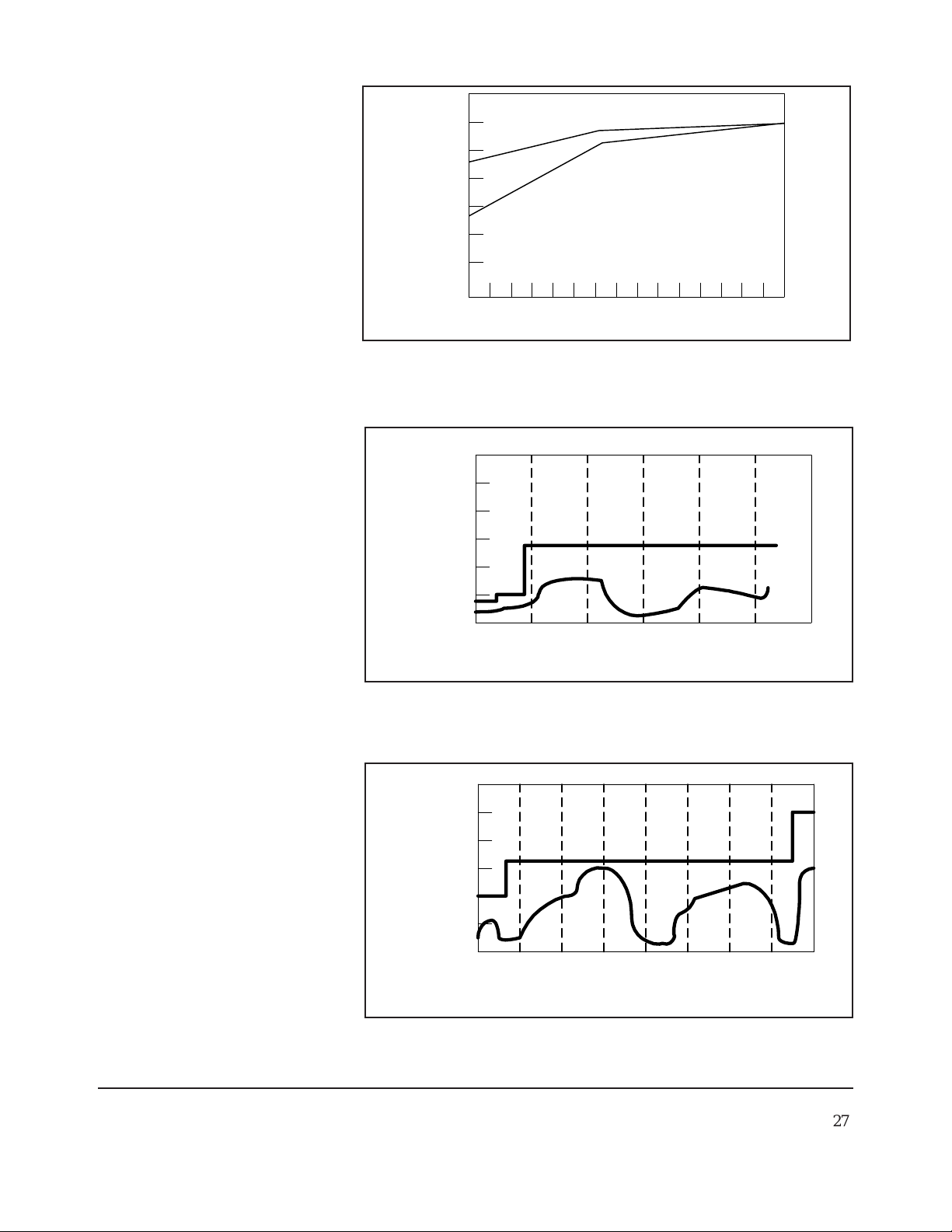
Page 33

Low Frequency Response and
28
Standing-Wave-Ratio (SWR) Data
The typical performance data that follows is not guaranteed, however, it represents a
large number of production units processed. Therefore, it is a good guideline for user
expectations. The worst case specifications are quite conservative in accordance with
Boonton's general policy.
Detailed SWR data is supplied with each sensor unit shipped against a customer order
to give the user specific information required to properly evaluate errors in a particular
application. Please consult the factory for optional units with more stringent
specifications.
The typical low frequency response for three sensor models are shown in Figures 4-1
through 4-3. Figures 4-4 through 4-10 represent SWR Data.
4
0
-1
-2
-3
-4
Response (dB)
-5
Figure 4-1. Model 51071 Low Frequency Response
-1
-2
-3
-4
Response (dB)
-5
0 dBm
-40 dBm
150
Frequency (MHz)
0
0 dBm
-40 dBm
10
150
Figure 4-2. Model 51072 Low Frequency Response
26 Power Sensor Manual
10
Frequency (MHz)
Page 34
0.0
29
-0.5
0 dBm
-1.0
-1.5
-2.0
Response (dB)
-2.5
0.1 10.3
-40 dBm
Frequency (MHz)
Figure 4-3. Model 51075 Low Frequency Response
2.0
1.8
1.6
1.4
SWR
1.2
1.0
51510 20 25
Spec
Frequency
(GHz)
Figure 4-4. Model 51071 SWR Data
2.0
1.8
1.6
1.4
SWR
1.2
1.0
51510 20 25
Frequency
Spec
3530
(GHz)
Figure 4-5. Model 51072 SWR Data
Power Sensor Manual 27
Page 35

2.0
30
1.8
1.6
1.4
SWR
1.2
1.0
51510 20 25
Spec
Frequency
(GHz)
Figure 4-6. Model 51075 SWR Data
2.0
1.8
1.6
1.4
SWR
1.2
Spec
1.0
51510 20 25
Frequency
(GHz)
Figure 4-7. Model 51078 SWR Data
2.0
1.8
1.6
1.4
SWR
1.2
1.0
51510 20 25
Spec
Frequency
(GHz)
Figure 4-8. Model 51100 SWR Data
28 Power Sensor Manual
Page 36

2.0
31
1.8
1.6
1.4
SWR
1.2
1.0
13245
Spec
Frequency
(GHz)
Figure 4-9. Model 51101 SWR Data
2.0
1.8
1.6
1.4
SWR
1.2
Spec
1.0
51510 20 25
Frequency
(GHz)
Figure 4-10. Model 51102 SWR Data
Power Sensor Manual 29
Page 37

Pulsed RF Power
32
5-1 Pulsed RF Power Operation
Although this manual discusses power sensors used with average responding power
meters, for rectangular pulsed RF signals, pulse power can be calculated from average
power if the duty cycle of the reoccurring pulse is known. The duty cycle can be found
by dividing the pulse width (T) by the period of the repetition frequency or by
multiplying the pulse width times the repetition frequency as shown in Figure 5-1.
5
P
P
P
p
avg
Duty Cycle =
P
p
=
Duty Cycle
1
=
T
r
f
T
Figure 5-1. Pulsed RF Operation
r
P
avg
T
T
r
t
This technique is valid for the entire dynamic range of Thermocouple Sensors and
allows very high pulse powers to be measured. For Diode Sensors, this technique is
valid only within the square-law region of the diodes.
30 Power Sensor Manual
Page 38

5-2 Pulsed RF Operation Thermocouple Sensors
33
Figure 5-2 shows the regions of valid duty cycle and pulse power that apply to the
Thermal Sensors. As the duty cycle decreases, the average power decreases for a
given pulse power and the noise becomes a limitation. Also, there is a pulse power
overload limitation. No matter how short the duty cycle is, this overload limitation
applies. Lastly, the average power cannot be exceeded (there is some headroom between
the measurement limitation and the burnout level of the sensor).
Since the detection process in Thermal Sensors is heat, Thermal Sensors can handle
pulse powers that are two orders of a magnitude larger than their maximum average
power. This makes them ideal for this application. The minimum pulse repetition
frequency for the Thermal Sensors is approximately 100 Hz.
30
Valid
20
measurement
region
Average
overload
limitation
(300mW)
Upper
measurement
limitation
(100mW Avg Power)
RMS Noise = 100 nW @ 4.8 sec filter
10
<0.1 dB
<0.2 dB
0
-10
Pulse Power (dBm)
Operation in this
-20
region not valid
<0.3 dB
Notes:
1
For 51200 and 51300 sensors,
add 20 dB to vertical axis. For
51201 and 51301 sensors, add
24 dB to vertical axis.
2
These accuracy figures are to
be added to the standard CW
accuracy figures.
-30
.001
.01 .1 1 10 100
Duty Cycle (%)
Figure 5-2. Pulsed Accuracy for Thermocouple Sensors
Power Sensor Manual 31
Page 39

5-3 Pulsed RF Operation Diode Sensors
34
Figure 5-3 shows the valid operating region for the Diode Sensors. As with Thermal
Sensors, the bottom end measurement is limited by noise, getting worse as the duty
cycle decreases. At the top end, the limitation is on pulse power because even a very
short pulse will charge up the detecting capacitors. The burnout level for Diode Sensors
is the same for the pulsed and CW waveforms. The minimum pulse repetition frequency
is 10 kHz.
0
-10
-20
-30
-40
Pulse Power (dBm)
-50
-60
<0.5 dB
Notes:
1
For 51015, 51016 and 51078
sensors, add 10, 20 and 30 dB
to the vertical axis respectively.
2
For 10 second filtering, drop
this line by 3 dB.
3
These figures are to be added
to the standard CW accuracy
figures.
Operation in this
region not valid
.001
.01 .1 1 10 100
<0.2 dB
<0.1 dB
222
RMS Noise = 65pW @ 2.8 sec filter
Duty Cycle (%)
Figure 5-3. Pulsed Accuracy for Diode Sensors
32 Power Sensor Manual
Page 40

Calculating Measurement Uncertainty
11
35
6-1 Introduction
This Section has been extracted from the 4530 manual since it provides examples using CW
and Peak Power sensors. As such, in calculating Power Measurement Uncertainty ,
specifications for the 4530 are used. If one of Boonton's other Power Meters are in use,
refer to its Instruction Manual for Instrument Uncertainty and Calibrator Uncertainty.
The 4530 Series includes a precision internal RF reference calibrator that is traceable to the
National Institute for Standards and Technology (NIST). When the instrument is maintained
according to the factory recommended one year calibration cycle, the calibrator enables you
to make highly precise measurements of CW and modulated signals. The error analyses in
this chapter assumes that the power meter is being maintained correctly and is within its valid
calibration period.
Measurement uncertainties are attributable to the instrument, calibrator, sensor, and impedance
mismatch between the sensor and the device under test (DUT). Individual independent
contributions from each of these sources are combined mathematically to quantify the upper
error bound and probable error. The probable error is obtained by combining the linear
(percent) sources on a root-sum-of-squares (RSS) basis.
6
Note that uncertainty figures for individual components may be provided given in either
percent or dB. The following formulas may be used to convert between the two units:
= (10(UdB/10) - 1) * 100 and UdB = 10 * Log10(1 + (U% / 100))
U
%
Section 6-2 outlines all the parameters that contribute to the power measurement uncertainty
followed by a discussion on the method and calculations used to express the uncertainty.
Section 6-3 continues discussing each of the uncertainty terms in more detail while presenting
some of their values.
Section 6-4 provides Power Measurement Uncertainty calculation examples for both CW and
Peak Power sensors with complete Uncertainty Budgets.
References used in the Power Measurement Uncertainty analysis are:
1. “ISO Guide to the Expression of Uncertainty in Measurement,”
Organization for Standardization, Geneva, Switzerland,
ISBN 92-67-10188-9, 1995.
2. “U.S. Guide to the Expression of Uncertainty in Measurement",
National Conference of Standards Laboratories, Boulder, CO 80301, 1996.
ANSI/NCSL Z540-2-1996,
`
Power Sensor Manual 33
Page 41

U
N
36
6-2 Uncertainty Contributions
The total measurement uncertainty is calculated by combining the following terms:
1. Instrument Uncertainty
2. Calibrator Level Uncertainty
3. Calibrator Mismatch Uncertainty
4. Source Mismatch Uncertainty
5. Sensor Shaping Error
6. Sensor Temperature Coefficient
7. Sensor Noise
8. Sensor Zero Drift
9. Sensor Calibration Factor Uncertainty
The formula for worst-case measurement uncertainty is:
U
WorstCase
where
through UNrepresent each of the worst-case uncertainty terms.
1
The worst-case approach is a very conservative method where the extreme condition of each
individual uncertainty is added to one another. If the individual uncertainties are independent
of one another, the probability of all being at the extreme condition is small. For this reason,
these uncertainties are usually combined using the RSS method. RSS is an abbreviation for
“root-sum-of-squares”. In this method, each uncertainty is squared, added to one another, and
the square root of the summation is calculated resulting in the Combined Standard Uncertainty.
The formula is:
= ( U
U
C
where U1 through UN represent normalized uncertainty based on the uncertainty's probaility
distribution. This calculation yields what is commonly refered to as the combined standard
uncertainty with a level of confidence of approximately 68%.
To gain higher levels of confidence an Expanded Uncertainty is often employed. Using a
coverage factor of 2 ( 2 * U
of approximately 95%.
6-3 Discussion of Uncertainty Terms
= U1 + U2 + U3 + U4 + ... U
2
2
2
1
+ U
+ U
2
3
) will provide an Expanded Uncertainty with a confidence level
C
+ U
2
+ ... U
4
N
2
0.5
)
Following is a discussion of each term, its definition, and how it is calculated.
Instrument Uncertainty. This term represents the amplification and digitization uncertainty
in the power meter, as well as internal component temperature drift. In most cases, this is very
small, since absolute errors in the circuitry are calibrated out by the AutoCal process. The
instrument uncertainty is 0.20% for the 4530 Series. (Refer to the Instruction Manual of the
instrument in use for instrument uncertainty.)
34 Power Sensor Manual
Page 42

Calibrator Level Uncertainty. This term is the uncertainty in the calibrator’s output level for
37
a given setting for calibrators that are maintained in calibrated condition. The figure is a
calibrator specification which depends upon the output level:
50MHz Calibrator Level Uncertainty:
At 0 dBm: ± 0.055 dB (1.27%)
+20 to -39 dBm: ± 0.075 dB (1.74%)
-40 to -60 dBm: ± 0.105 dB (2.45%)
1GHz Calibrator Level Uncertainty:
± (0.065 dB (1.51%) at 0 dBm + 0.03 dB (0.69%) per 5 dB from 0 dBm)
The value to use for calibration level uncertainty depends upon the sensor calibration
technique used. If AutoCal was performed, the calibrator’s uncertainty at the measurement
power level should be used. For sensors calibrated with FixedCal, the calibrator is only used
as a single-level source, and you should use the calibrator’s uncertainty at the FixedCal level,
(0dBm, for most sensors). This may make FixedCal seem more accurate than AutoCal at
some levels, but this is usually more than offset by the reduction in shaping error afforded by
the AutoCal technique. (Refer to the Instruction Manual of the instrument in use for
calibrator level uncertainty.)
Calibrator Mismatch Uncertainty. This term is the mismatch error caused by impedance
differences between the calibrator output and the sensor’s termination. It is calculated from
the reflection coefficients of the calibrator (D
) and sensor (D
CAL
) at the calibration
SNSR
frequency with the following equation:
Calibrator Mismatch Uncertainty = ±2 * D
CAL
* D
SNSR
* 100 %
The calibrator reflection coefficient is a calibrator specification:
Internal Calibrator Reflection Coefficient (D
External 2530 Calibrator Reflection Coefficient (D
The sensor reflection coefficient, D
is frequency dependent, and may be looked up in
SNSR
): 0.024 (at 50MHz)
CAL
): 0.091 (at 1GHz)
CAL
Section 2 of this manual. (Refer to the Instruction Manual of the instrument in use for
calibrator SWR specifications.)
Source Mismatch Uncertainty. This term is the mismatch error caused by impedance
differences between the measurement source output and the sensor’s termination. It is
calculated from the reflection coefficients of the source (D
) and sensor (D
SRCE
SNSR
) at
the measurement frequency with the following equation:
Source Mismatch Uncertainty = ±2 * D
SRCE
* D
SNSR
* 100 %
The source reflection coefficient is a characteristic of the RF source under test. If only the
SWR of the source is known, its reflection coefficient may be calculated from the source
SWR using the following equation:
Source Reflection Coefficient (D
) = (SWR - 1) / (SWR + 1)
SRCE
Power Sensor Manual 35
Page 43

The sensor reflection coefficient, D
38
is frequency dependent, and can be referenced in
SNSR
Section 2 of this manual. For most measurements, this is the single largest error term, and care
should be used to ensure the best possible match between source and sensor. Figure 6-1. plots
Mismatch Uncertainty based on known values of both source and sensor SWR.
Sensor Shaping Error. This term is sometimes called "linearity error", and is the residual
non-linearity in the measurement after an AutoCal has been performed to characterize the
"transfer function" of the sensor (the relationship between applied RF power, and sensor
output, or shaping). Calibration is performed at discrete level steps and is extended to all
levels. Generally, sensor shaping error is close to zero at the autocal points, and increases in
between due to imperfections in the curve-fitting algorithm.
An additional component of sensor shaping error is due to the fact that the sensor's transfer
function may not be identical at all frequencies. The published shaping error includes terms
to account for these deviations. If your measurement frequency is close to your AutoCal
frequency, it is probably acceptable to use a value lower than the published uncertainty in your
calculations.
For CW sensors using the fixed-cal method of calibrating, the shaping error is higher because
it relies upon stored "shaping coefficients" from a factory calibration to describe the shape of
the transfer function, rather than a transfer calibration using a precision power reference at the
current time and temperature. For this reason, use of the AutoCal method is recommended for
CW sensors rather than simply performing a FixedCal. The shaping error for CW sensors
using the FixedCal calibration method is listed as part of the "Sensor Characteristics"
outlined in Section 2 of this manual. If the AutoCal calibration method is used with a CW
sensor, a fixed value of 1.0% may be used for all signal levels.
All peak power sensors use the AutoCal method only. The sensor shaping error for peak
sensors is also listed in Section 2 of this manual.
Sensor Temperature Coefficient. This term is the error which occurs when the sensor's
temperature has changed significantly from the temperature at which the sensor was AutoCal'd.
This condition is detected by the Model 4530 and a "temperature drift" message warns the
operator to recalibrate the sensor for drift exceeding ± 4 °C on non-temperature compensated
peak sensors.
Temperature compensated peak sensors have a much smaller temperature coefficient, and a
much larger temperature deviation, ± 30 °C is permitted before a warning is issued. For these
sensors, the maximum uncertainty due to temperature drift from the autocal temperature is:
Temperature Error = ± 0.04dB (0.93%) + 0.003dB (0.069%) / °C
Note that the first term of this equation is constant, while the second term (0.069%) must be
multiplied by the number of degrees that the sensor temperature has drifted from the AutoCal
temperature.
CW sensors have no built-in temperature detectors, so it is up to the user to determine the
temperature change from AutoCal temperature. Temperature drift for CW sensors is
determined by the temperature coefficient of the sensor. This figure is 0.01dB (0.23%) per
degreeC for the 51075 and many other CW sensors. Refer to Section 2 for the exact figure to
36 Power Sensor Manual
Page 44

Mismatch Uncertainty
39
SWR -1 Relative Power Uncertainty
p =
SWR +1 P.U. = (1 +/- p p )
L
S
p = Source SWR
Where p = Load SWR
L
S
Chart
Figure 6-1. Mismatch Uncertainty
Power Sensor Manual 37
Page 45

use. Sensor temperature drift uncertainty may be assumed to be zero for sensors operating
40
exactly at the calibration temperature.
Sensor Noise. The noise contribution to pulse measurements depends on the number of
samples averaged to produce the power reading, which is set by the "averaging" menu setting.
For continuous measurements with CW sensors, or peak sensors in modulated mode, it
depends on the integration time of the measurement, which is set by the "filter" menu setting.
In general, increasing filtering or averaging reduces measurement noise. Sensor noise is
typically expressed as an absolute power level. The uncertainty due to noise depends upon the
ratio of the noise to the signal power being measured. The following expression is used to
calculate uncertainty due to noise:
Noise Error = ± Sensor Noise (in watts) / Signal Power (in watts) * 100 %
The noise rating of a particular power sensor may be found in Section 2 of this manual. It may
be necessary to adjust the sensor noise for more or less filtering or averaging, depending upon
the application. As a general rule (within a decade of the datasheet point), noise is inversely
proportional to the filter time or averaging used. Noise error is usually insignificant when
measuring at high levels (25dB or more above the sensor's minimum power rating).
Sensor Zero Drift. Zero drift is the long-term change in the zero-power reading that is not a
random, noise component. Increasing filter or averaging will not reduce zero drift. For lowlevel measurements, this can be controlled by zeroing the meter just before performing the
measurement. Zero drift is typically expressed as an absolute power level, and its error
contribution may be calculated with the following formula:
Zero Drift Error = ± Sensor Zero Drift (in watts) / Signal Power (in watts) *100 %
The zero drift rating of a particular power sensor may be found in Section 2 of this manual.
Zero drift error is usually insignificant when measuring at high levels (25dB or more above the
sensor's minimum power rating). The drift specification usually indicates a time interval such
as one hour. If the time since performing a sensor Zero or AutoCal is very short, the zero
drift is greatly reduced
Sensor Calibration Factor Uncertainty. Sensor frequency calibration factors ("calfactors")
are used to correct for sensor frequency response deviations. These calfactors are characterized during factory calibration of each sensor by measuring its output at a series of test
frequencies spanning its full operating range, and storing the ratio of the actual applied power
to the measured power at each frequency. This ratio is called a calfactor. During measurement
operation, the power reading is multiplied by the calfactor for the current measurement
frequency to correct the reading for a flat response.
The sensor calfactor uncertainty is due to uncertainties encountered while performing this
frequency calibration (due to both standards uncertainty, and measurement uncertainty), and is
different for each frequency. Both worst case and RSS uncertainties are provided for the
frequency range covered by each sensor, and are listed in Section 3 of this manual.
If the measurement frequency is between sensor calfactor entries, the most conservative
approach is to use the higher of the two corresponding uncertainty figures. It is also be
possible to estimate the figure by linear interpolation.
38 Power Sensor Manual
Page 46

If the measurement frequency is identical to the AutoCal frequency, a calfactor uncertainty of
t
l
41
zero should be used, since any absolute error in the calfactor cancels out during AutoCal. At
frequencies that are close to the AutoCal frequency, the calfactor uncertainty is only partially
cancelled out during AutoCal, so it is generally acceptable to take the uncertainty for the next
closest frequency, and scale it down.
6-4 Sample Uncertainty Calculations
The following examples show calculations for two measurement applications - one using a CW
sensor (Model 51075), and the other with a peak power sensor (Model 57518). The figures
used in these examples are meant to show the general techniques, and do not apply to all
applications. Some "common sense" assumptions have been made to illustrate the fact that
uncertainty calculation is not an exact science, and requires some understanding of your
specific measurement conditions.
Typical Example #1: Model 51075 CW Power Sensor
Measurement conditions:
Source Frequency: 10.3 GHz
Source Power: -55 dBm (3.16 nW)
Source SWR : 1.50 (reflection coefficient = 0.2) at 10.3 GHz
AutoCal Source: Internal 50MHz Calibrator
AutoCal Temperature: 25 °C
Current Temperature: 25 °C
In this example, we will assume that an AutoCal has been performed on the sensor
immediately before the measurement. This will reduce certain uncertainty terms, as discussed
below.
Step 1: The Instrument Uncertainty figure for the 4530 Series is ±0.20%. Since a portion of
this figure is meant to include temperature drift of the instrument, and we know an AutoCal has
just been performed, we'll estimate (for lack of more detailed, published information) that the
instrument uncertainty is ± 0.10 %, or half the published figure.
Instrumen
= ± 0.10%
U
Step 2: The Calibrator Level Uncertainty for the power meter's internal, 50MHz calibrator
may be read from the calibrator's specification. It is ±0.105dB, or ±2.45% at a level of -55
dBm.
CalLeve
= ± 2.45%
U
Power Sensor Manual 39
Page 47

Step 3: The Calibrator Mismatch Uncertainty is calculated using the formula in the previous
h
r
N
42
section, using the internal 50MHz calibrator's published figure for D
value D
from the SWR specification on the 51075's datasheet.
SNSR
and calculating the
CAL
D
D
CAL
SNSR
= 0.024 (internal calibrator's reflection coefficient at 50MHz)
= (1.15 - 1) / (1.15 + 1) = 0.070
(calculated reflection coefficient of 51075, max SWR = 1.15 at 50MHz)
U
CalMismatch
= ± 2 * D
CAL
* D
SNSR
* 100 %
= ± 2 * 0.024 * 0.070 * 100 %
= ± 0.34%
Step 4: The Source Mismatch Uncertainty is calculated using the formula in the previous
section, using the DUT's specification for D
and calculating the value D
SRCE
SNSR
from the
SWR specification on the 51075's datasheet.
D
D
SRCE
SNSR
= 0.20 (source reflection coefficient at 10.3GHz)
= (1.40 - 1) / (1.40 + 1) ) = 0.167
(calculated reflection coefficient of 51075, max SWR = 1.40 at 10.3GHz)
U
SourceMismatc
= ± 2 * D
SRCE
* D
SNSR
* 100 %
= ± 2 * 0.20 * 0.167 * 100 %
= ± 6.68%
Step 5: The uncertainty caused by Sensor Shaping Error for a 51075 CW sensor that has been
calibrated using the AutoCal method can be assumed to be 1.0%, as per the discussion in the
previous section.
U
ShapingErro
= ± 1.0 %
Step 6: The Sensor Temperature Drift Error depends on how far the temperature has drifted
from the sensor calibration temperature, and the temperature coefficient of the sensor. In this
example, an AutoCal has just been performed on the sensor, and the temperature has not
drifted at all, so we can assume a value of zero for sensor temperature drift uncertainty.
U
SnsrTempDrift
= ± 0.0 %
Step 7: This is a relatively low-level measurement, so the noise contribution of the sensor
must be included in the uncertainty calculations. We'll assume default filtering. The signal
level is -55dBm, or 3.16nW. The RMS noise specification for the 51075 sensor is 30pW,
from Section 2. Noise uncertainty is the ratio of these two figures.
U
oiseError
= ± Sensor Noise (in watts) / Signal Power (in watts)
= ± 30.0e-12 / 3.16e-9 * 100 %
= ± 0.95%
40 Power Sensor Manual
Page 48

Step 8: The Sensor Zero Drift calculation is very similar to the noise calculation. For sensor
t
r
43
zero drift, the datasheet specification for the 51075 sensor is 100pW, so we'll take the liberty
of cutting this in half to 50pW, since we just performed an AutoCal, and it's likely that the
sensor hasn't drifted much.
U
= ± Sensor Zero Drift (in watts) / Signal Power (in watts)
ZeroDrif
= ± 50.0e-12 / 3.16e-9 * 100 %
= ± 1.58%
Step 9: The Sensor Calfactor Uncertainty is calculated from the uncertainty values specified
in Section 3 of this manual. There is no entry for 10.3GHz, so we'll have to look at the two
closest entries. At 10GHz, the calfactor uncertainty is 4.0 % and at 11GHz it is 4.3 %.
A linear interpolation must be done to determine the Calfactor at 10.3 GHz. The uncertainty is
then;
U
= [ ( F - F1 ) * (( CF2 - CF1 ) / ( F2 - F1 )) ] + CF
CalFacto
1
where; F = 10.3
= 10 CF1 = 4.0
F
1
F
= 11 CF2 = 4.3
2
= [ ( 10.3 - 10.0 ) * (( 4.3 - 4.0 ) / ( 11.0 - 10.0 )) ] + 4.0
= [ ( 0.3 ) * (( 0.3 ) / ( 1.0 )) ] + 4.0
= [ ( 0.3 ) * ( 0.3 ) ] + 4.0
= 4.09 %
Step 10: Now that each of the individual uncertainty terms has been determined, we can
create an uncertainty budget and calculate the combined standard uncertainty (Uc) .
Source of Symbol
Uncertainty
Instrument
Value
(+/- %)
I
0.10 normal
Probabilty
Distribution
Divisor Ustd
(+/- %)
2 0.05
Calibrator
Level
Mismatch
M
R
C
2.45
0.34
rectangular
U-shaped
( 3 )
( 2 )
0.5
0.5
1.41
0.24
Source
Mismatch
M
S
6.68
U-shaped
( 2 )
0.5
4.72
Sensor
Shaping
Temp. Drift
Noise
Zero drift
Cal Factor
S
T
N
1.00
0
0.95 normal
Z 1.58
rectangular
rectangular
rectangular
K 4.09 normal
0.5
( 3 )
0.5
( 3 )
2 0.48
0.5
( 3 )
2 2.05
0.58
0.00
0.91
Combined Standard
Uncertainty
Expanded
Uncertainty
Uc
U
normal
normal
(k=2)
5.47
10.94
Power Sensor Manual 41
Page 49

From the previous example, it can be seen that the two largest contributions to the combined
t
44
standard uncertainty are the source mismatch, and the sensor calfactor.
Typical Example #2: Model 57518 Peak Power Sensor
Measurement conditions:
Source Frequency: 900 MHz
Source Power: 13 dBm (20mW)
Source SWR : 1.12 (reflection coefficient = 0.057) at 900 MHz
AutoCal Source: External 2530 1GHz Calibrator
AutoCal Temperature: 38C
Current Temperature: 49C
In this example, we will assume that an AutoCal was performed on the sensor earlier in the
day, so time and temperature drift may play a role in the uncertainty.
Step 1: The Instrument Uncertainty figure for the 4530 Series is ±0.20%. Since it has been a
while since AutoCal, we’ll use the published figure.
Instrumen
= ± 0.20%
U
Step 2: The Calibrator Level Uncertainty for the Model 2530 1GHz external calibrator may
be calculated from the calibrator’s specification. The 0dBm uncertainty is 0.065dB, or 1.51%.
To this figure, we must add 0.03dB or 0.69% per 5dB step from 0dBm. 13dBm is 2.6 5dB
steps (13/5) away from 0dBm. Any fraction must always be rounded to the next highest whole
number, so we’re 3 steps away.
U
CalLevel
= ± ( 1.51% + ( 3 * 0.69% ))
= ± 3.11%
Step 3: The Calibrator Mismatch Uncertainty is calculated using the formula in the previous
section, using the 2530 calibrator’s published figure for D
D
from the SWR specification outlined in Section 2 of this manual.
SNSR
D
D
CAL
SNSR
= 0.091 (external 2530 calibrator’s reflection coefficient at 1GHz)
= (1.15 - 1) / (1.15 + 1) = 0.070
and calculating the value
CAL
(calculated reflection coefficient of 57518, max SWR = 1.15 at 1 GHz)
U
CalMismatch
= ± 2 * D
CAL
* D
SNSR
* 100 %
= ± 2 * 0.091 * 0.070 * 100 %
= ± 1.27%
42 Power Sensor Manual
Page 50

Step 4: The Source Mismatch Uncertainty is calculated using the formula in the previous
h
t
N
t
45
section, using the DUT’s specification for D
and calculating the value D
SRCE
SNSR
from the
SWR specification found in Section 2.
D
D
= 0.057 (source reflection coefficient at 900 MHz)
SRCE
= (1.15 - 1) / (1.15 + 1) )
SNSR
= 0.070
(calculated reflection coefficient of 57518, max SWR = 1.15 at 0.9 GHz)
U
SourceMismatc
= ± 2 * D
SRCE
* D
SNSR
* 100 %
= ± 2 * 0.057 * 0.070 * 100 %
= ± 0.80%
Step 5: The uncertainty caused by Sensor Shaping Error for a 57518 peak sensor is 4% at
all levels (from table 2-2). But since we’re measuring at 900MHz, which is very close to the
1GHz AutoCal frequency, we’ll assume that the frequency-dependent portion of the shaping
error becomes very small, and we’ll estimate that 2% remains.
U
ShapingError
= ± 2.0 %
Step 6: The Sensor Temperature Drift Error depends on how far the temperature has drifted
from the sensor calibration temperature, and the temperature coefficient of the sensor. In our
case, we are using a temperature compensated sensor, and the temperature has drifted by 11
degrees C (49C - 38C) from the AutoCal temperature. We will use the equation in the
previous section to calculate sensor temperature drift uncertainty.
U
SnsrTempDrif
= ± ( 0.93% + 0.069% / °C)
= ± ( 0.93 + ( 0.069 * 11.0 ) ) %
= ± 1.69 %
Step 7: This is a relatively high-level measurement, so the noise contribution of the sensor is
probably negligible, but we’ll calculate it anyway. We’ll assume modulate mode with default
filtering. The signal level is 13dBm, or 20mW. The “noise and drift” specification for the
57518 sensor is 50nW, from Table 2-2 (Peak Power Sensor Characteristics).
Noise uncertainty is the ratio of these two figures.
U
= ± Sensor Noise (in watts) / Signal Power (in watts)
oise&Drif
= ± 50.0e-9 / 20.0e-3 * 100 %
= ± 0.0003 %
Step 8: A separate Sensor Zero Drift calculation does not need to be performed for peak
sensors, since “noise and drift” are combined into one specification, so we’ll just skip this
step.
Power Sensor Manual 43
Page 51

Step 9: The Sensor Calfactor Uncertainty needs to be interpolated from the uncertainty
r
o
46
values given in Table 3-2 (Peak Power Sensor Calibration Factor Uncertainty). At 1 GHz, the
sensor’s calfactor uncertainty is 1.7 %, and at 0.5 GHz it is 1.6 %. Note, however, that
we are performing our AutoCal at a frequency of 1 GHz, which is very close to the
measurement frequency. This means that the calfactor uncertainty cancels to zero at 1 GHz.
We’ll use linear interpolation between 0.5 GHz and 1 GHz to estimate a value. 900 MHz
is only 20% (one fifth) of the way from 1GHz down to 500MHz, so the uncertainty figure at
0.5 GHz can be scaled by one fifth.
U
= [ ( F - F1 ) * (( CF2 - CF1 ) / ( F2 - F1 )) ] + CF
CalFacto
1
where; F = 0.9
= 0.5 CF1 = 1.6
F
1
F
= 1.0 CF2 = 0.0
2
= [ ( 00.9 - 00.5 ) * (( 0.0 - 1.6 ) / ( 1.0 - 0.5 )) ] + 1.6
= [ ( 0.4 ) * (( -1.6 ) / ( 0.5 )) ] + 1.6
= [ ( 0.4 ) * ( -1.6 ) ] + 1.6
= 0.32 %
Step 10: Now that each of the individual uncertainty terms has been determined, we can
create an uncertainty budget and calculate the combined standard uncertainty (Uc) .
Source of Symbol
Uncertainty
Instrument
Value
(+/- %)
I 0.2 normal
Probabilty
Distribution
Divisor Ustd
(+/- %)
2 0.10
Calibrator
Level
Mismatch
R 3.11 rectangular
M
C
1.27 U-shaped
( 3 )
( 2 )
0.5
0.5
1.80
0.90
Source
Mismatch
M
S
0.80 U-shaped
( 2 )
0.5
0.57
Sensor
Shaping
Temp. Drift
Noise
S 2.00 rectangular
T 1.69 rectangular
N 0.03 normal
0.5
( 3 )
0.5
( 3 )
2 0.02
1.15
0.98
Cal Factor
Combined Standard
Uncertainty
Expanded
Uncertainty
K 0.32 normal
Uc normal
U normal
(k=2)
2 0.16
2.58
5.17
From this example, different uncertainty terms dominate. Since the measurement is close t
the calibration frequency, and matching is rather good, the shaping and level errors are the
largest. The Expanded Uncertainty of 5.17 % translates to an uncertainty of about 0.22 dB
in the reading.
44 Power Sensor Manual
Page 52

Warranty
47
Power Sensor Manual
Boonton Electronics (Boonton) warrants its products to the original Purchaser to be free
from defects in material and workmanship for a period of one year from date of shipment
for instrument, and for one year from date of shipment for probes, power sensors and
accessories. Boonton further warrants that its instruments will perform within all current
specifications under normal use and service for one year from date of shipment. These
warranties do not cover active devices that have given normal service, sealed assemblies
which have been opened or any item which has been repaired or altered without Boonton's
authorization.
Boonton's warranties are limited to either the repair or replacement, at Boonton's option,
of any product found to be defective under the terms of these warranties.
There will be no charge for parts and labor during the warranty period. The Purchaser
shall prepay shipping charges to Boonton or its designated service facility and shall
return the product in its original or an equivalent shipping container. Boonton or its
designated service facility shall pay normal ground shipping charges to return the product
to the Purchaser. The Purchaser shall pay all shipping charges, duties and taxes if a
product is returned to Boonton from outside of the United States.
7
THE FOREGOING WARRANTIES ARE IN LIEU OF ALL OTHER WARRANTIES,
EXPRESSED OR IMPLIED, INCLUDING, BUT NOT LIMITED TO, THE IMPLIED
WARRANTIES OF MERCHANTABILITY AND FITNESS FOR A PARTICULAR
PURPOSE. Boonton shall not be liable to any incidental or consequential damages, as
defined in Section 2-715 of the Uniform Commercial Code, in connection with the products
covered by the foregoing warranties.
45
 Loading...