

Page 1
YOU'RE HEARD, LOUD AND CLEAR.
Instruction Manual
Bandpass Cavity Filters
6 5/8” and 10” Diameter
Manual Part Number
7-9145
8625 Industrial Parkway, Angola, NY 14006 Tel: 716-549-4700 Fax: 716-549-4772 sales@birdrf.com www.bird-technologies.com
Page 2

Warranty
This warranty applies for one year from shipping date.
TX RX Systems Inc. warrants its products to be free from defect in material and workmanship at the time of shipment.
Our obligation under warranty is limited to replacement or repair, at our option, of any such products that shall have
been defective at the time of manufacture. TX RX Systems Inc. reserves the right to replace with merchandise of
equal performance although not identical in every way to that originally sold. TX RX Systems Inc. is not liable for dam-
age caused by lightning or other natural disasters. No product will be accepted for repair or replacement without our
prior written approval. The purchaser must prepay all shipping charges on returned products. TX RX Systems Inc.
shall in no event be liable for consequential damages, installation costs or expense of any nature resulting from the
purchase or use of products, whether or not they are used in accordance with instructions. This warranty is in lieu of all
other warranties, either expressed or implied, including any implied warranty or merchantability of fitness. No representative is authorized to assume for TX RX Systems Inc. any other liability or warranty than set forth above in connection with our products or services.
TERMS AND CONDITIONS OF SALE
PRICES AND TERMS:
Prices are FOB seller’s plant in Angola, NY domestic packaging only, and are subject to change without notice. Federal, State and local sales or excise taxes are not included in prices. When Net 30 terms are applicable, payment is
due within 30 days of invoice date. All orders are subject to a $100.00 net minimum.
QUOTATIONS:
Only written quotations are valid.
ACCEPTANCE OF ORDERS:
Acceptance of orders is valid only when so acknowledged in writing by the seller.
SHIPPING:
Unless otherwise agreed at the time the order is placed, seller reserves the right to make partial shipments for which
payment shall be made in accordance with seller’s stated terms. Shipments are made with transportation charges collect unless otherwise specified by the buyer. Seller’s best judgement will be used in routing, except that buyer’s routing
is used where practicable. The seller is not responsible for selection of most economical or timeliest routing.
CLAIMS:
All claims for damage or loss in transit must be made promptly by the buyer against the carrier. All claims for shortages
must be made within 30 days after date of shipment of material from the seller’s plant.
SPECIFICATION CHANGES OR MODIFICATIONS:
All designs and specifications of seller’s products are subject to change without notice provided the changes or modifications do not affect performance.
RETURN MATERIAL:
Product or material may be returned for credit only after written authorization from the seller, as to which seller shall
have sole discretion. In the event of such authorization, credit given shall not exceed 80 percent of the original purchase. In no case will Seller authorize return of material more than 90 days after shipment from Seller’s plant. Credit
for returned material is issued by the Seller only to the original purchaser.
ORDER CANCELLATION OR ALTERATION:
Cancellation or alteration of acknowledged orders by the buyer will be accepted only on terms that protect the seller
against loss.
NON WARRANTY REPAIRS AND RETURN WORK:
Consult seller’s plant for pricing. Buyer must prepay all transportation charges to seller’s plant. Standard shipping policy set forth above shall apply with respect to return shipment from TX RX Systems Inc. to buyer.
DISCLAIMER
Product part numbering in photographs and drawings is accurate at time of printing. Part number labels on TX RX
products supersede part numbers given within this manual. Information is subject to change without notice.
Bird Technologies Group TX RX Systems Inc.
Page 3

Manual Part Number 7-9145
Copyright © 1996 TX RX Systems, Inc.
First Printing: August 1996
Version Number Version Date
1 08/05/96
Symbols Commonly Used
WARNING
CAUTION or ATTENTION
High Voltage
Use Safety Glasses
ESD Elecrostatic Discharge
Hot Surface
Electrical Shock Hazard
NOTE
Important Information
Bird Technologies Group TX RX Systems Inc.
Page 4

Page 5
dBm
10
1
MHZ/DIV
98.00
MHZ
300
KHZ/RES
0
-10
-20
-30
-40
-50
-60
-70
INSERTION LOSS
40 dB ATT
PASS FREQUENCY
GEN 0 dBM
10 MSEC
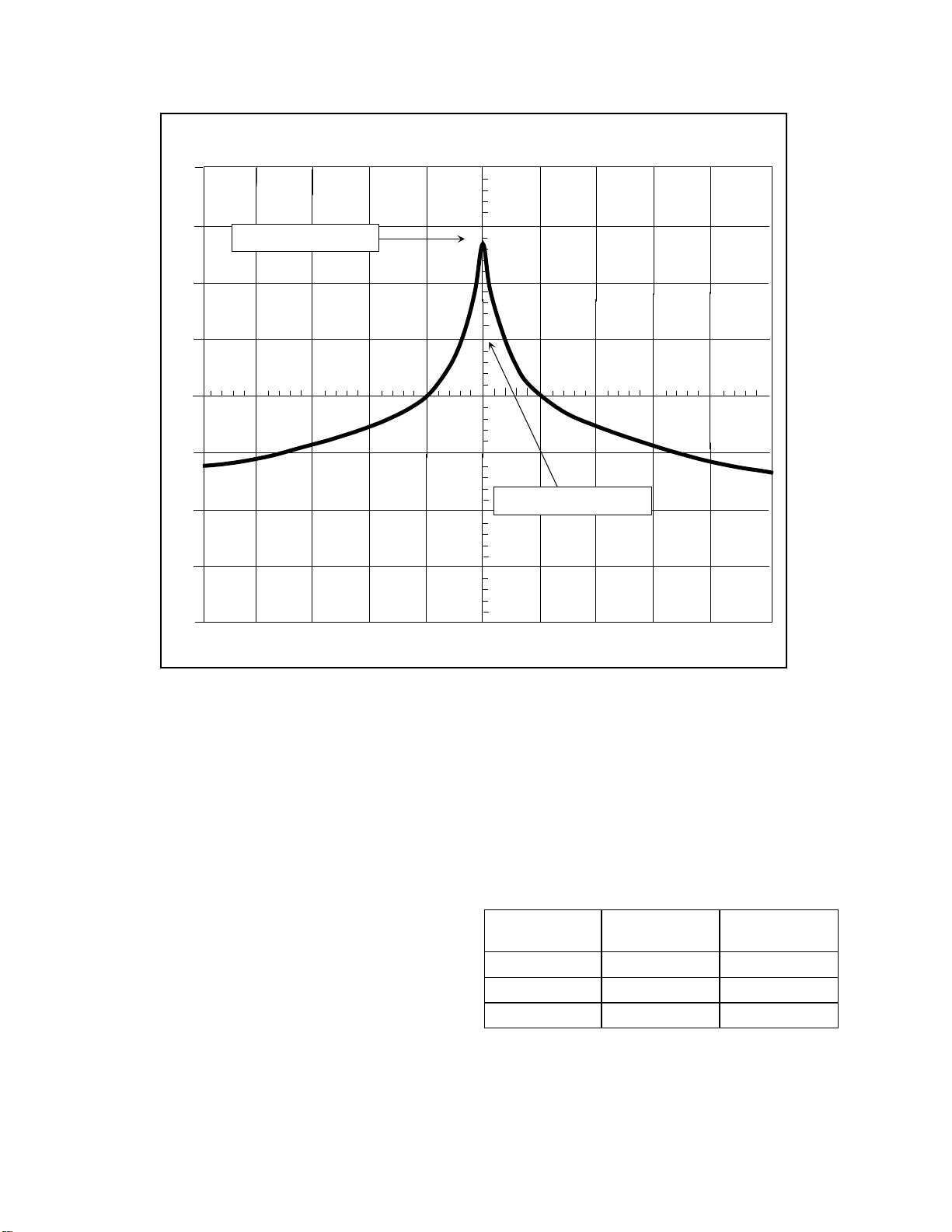
Figure 1: Spectrum Analyzer / Tracking Generator display of the Bandpass filter.
Response curve shown for model # 11-29-01 (88 - 108 MHz)
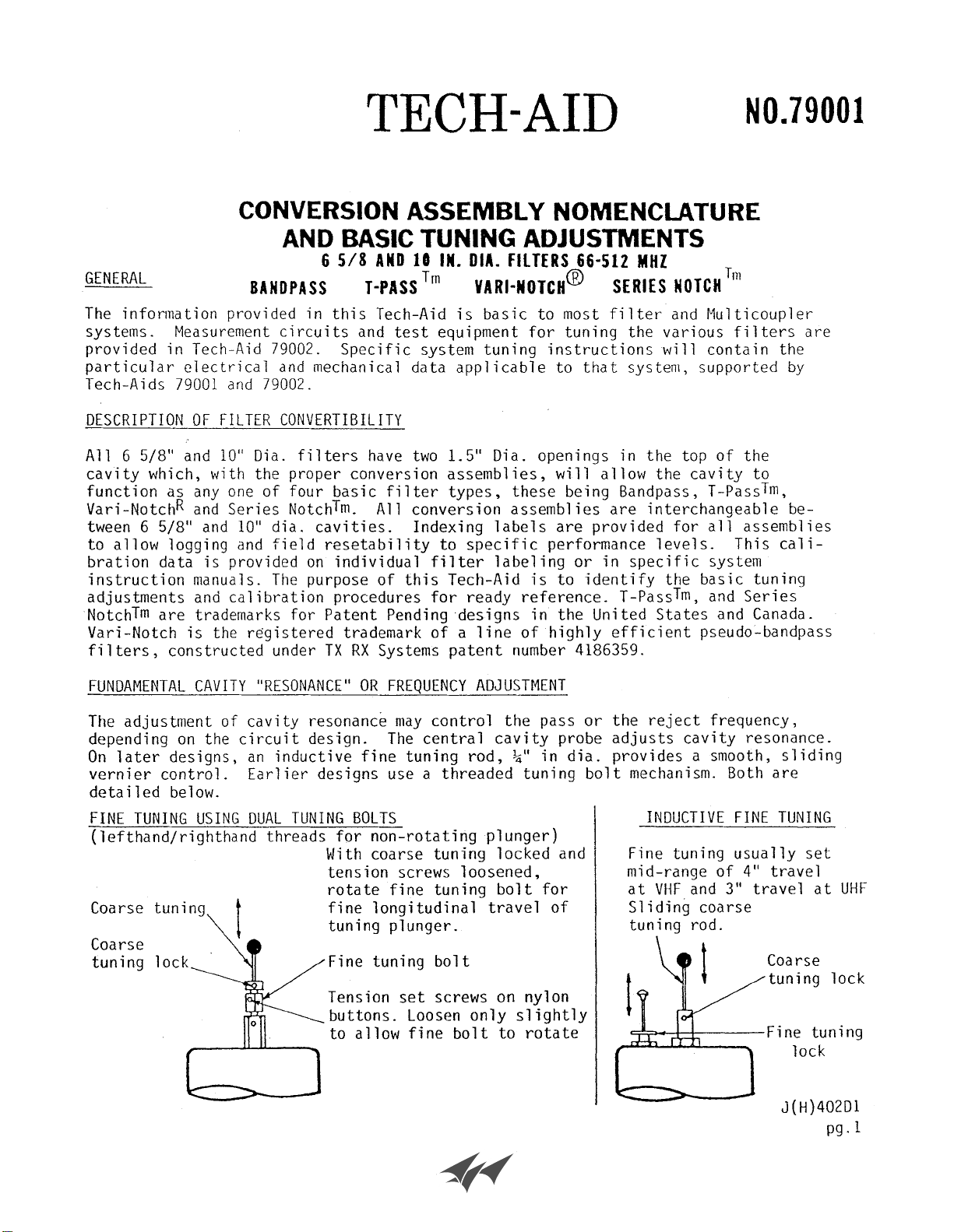
GENERAL DESCRIPTION
The Bandpass cavity filter passes one narrow band
of frequencies (
passband
) and attenuates all
others with increasing attenuation above and below
the pass frequency. Bandpass filters have
adjustable selectivity characteristics which allows a
trade off between insertion loss and selectivity, with
a higher loss giving greater selectivity. Maximum
power handling is determined by the insertion loss
setting. A variety of models are available that cover
the range of frequencies from 30 to 960 MHz. The
portion of the frequency range that each model will
tune across is determined by the cavity's physical
length.
Either 6-5/8" or 10" diameter resonator shells may
be used to construct the filters. The difference
between the two sizes determines the filters
selectivity and it's maximum power dissipation. The
10" diameter filters have slightly higher selectivity
compared to the 6-5/8" models and can safely
dissipate up to 40 Watts of RF Power. The 6-5/8"
filters can dissipate up to 30 Watts. Maximum input
power for the 6" and 10" diameter filters is listed in
table 1. When a filter is operated above 1.0 dB loss
in transmitter applications, we recommend
inserting a ferrite isolator between a transmitter
and the Bandpass filter because the VSWR may
exceed 1.5 : 1.
Insertion loss 6" diameter
Power Rating
10" diameter
Power Rating
0.5 dB 275 Watts 368 Watts
1.0 dB 146 Watts 194 Watts
3.0 dB 60 Watts 80 Watts
Table 1: Input power ratings.
There are two adjustable parameters found in a
bandpass filter including the pass frequency and
the insertion loss. Each of these parameters is
TX RX Systems Inc. Manual 7-9145-1 08/05/96 Page 1
Page 6
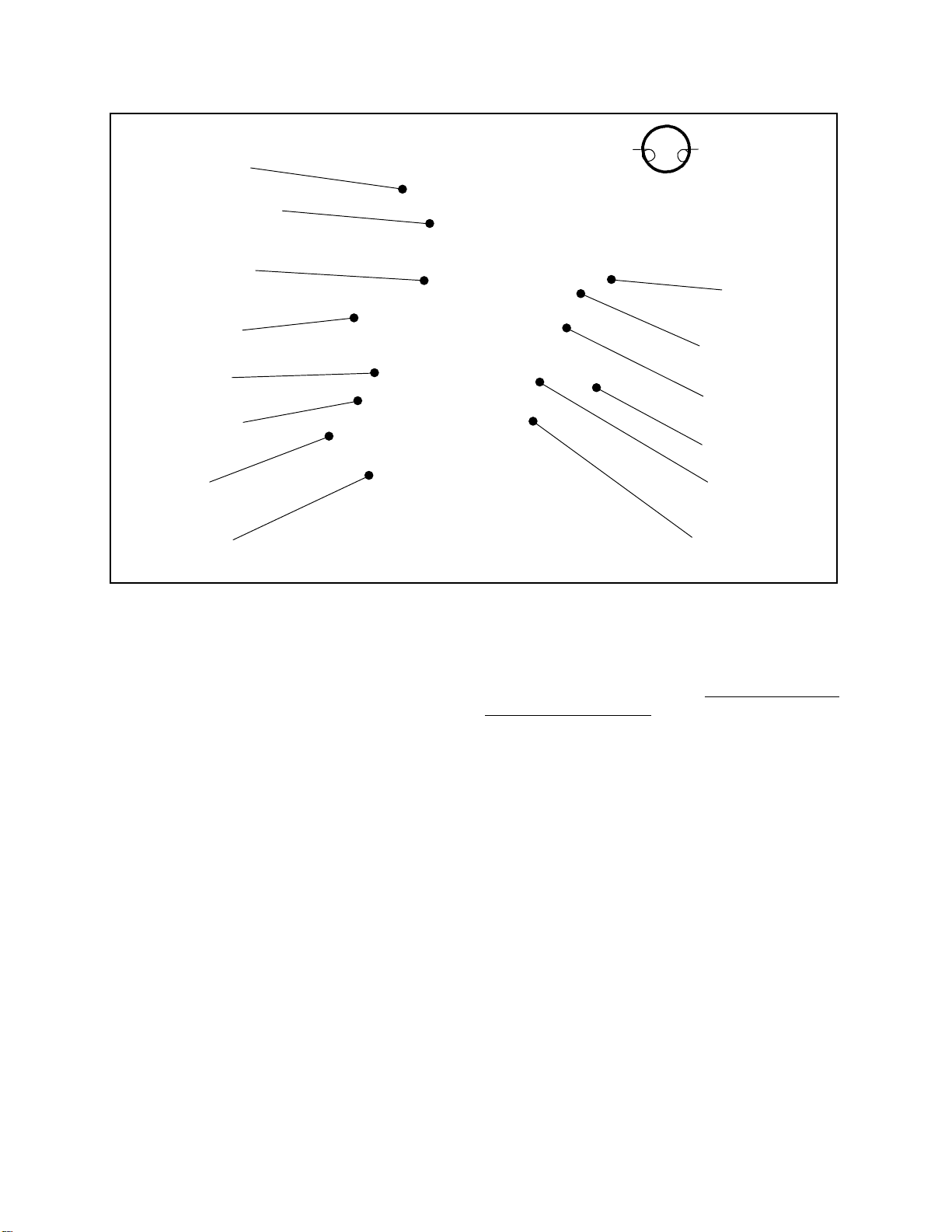
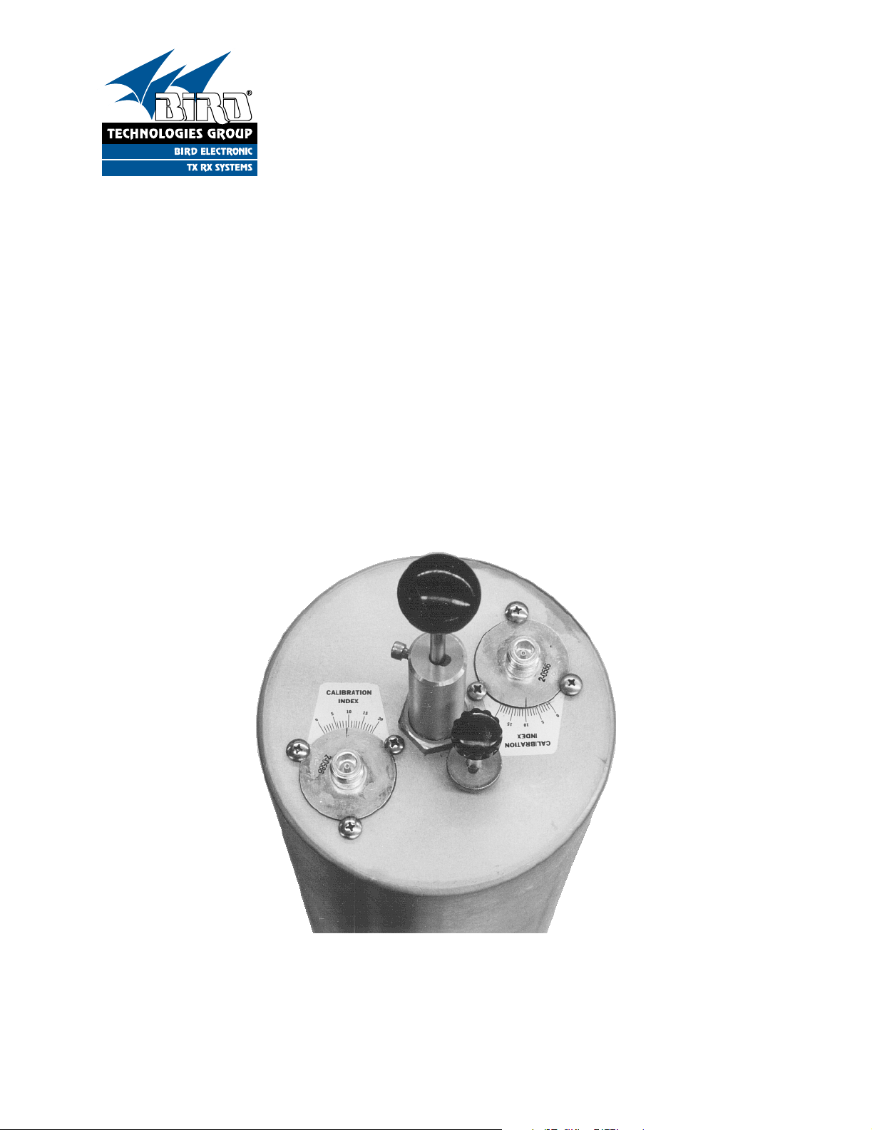
Cavity Resonator
Coarse Tuning Rod
Coarse Tuning Lock
10-32 Cap Screw
Calibration Index
Calibration Mark
Input/Output Port
Loop Plate
Assembly
Schematic
Symbol
Loop Plate
Assembly
Input/Output Port
Calibration Mark
Calibration Index
Fine Tuning Rod
Loop Plate
Hold Down Screws
Figure 2: The Bandpass filter.
labeled in figure 1. All of the physical components
of the filter are labeled in figure 2, with the
adjustable parts shown in emboldened italics.
Coarse and fine tuning rods are used to adjust the
pass (resonant) frequency. The insertion loss is
changed by rotating the two loop plate assemblies.
TUNING
Required Equipment
The following equipment or its equivalent is
recommended in order to properly perform the
tuning adjustments for the Bandpass filter.
1. IFR A-7550 Spectrum Analyzer with optional
Tracking Generator installed.
2. Double shielded coaxial cable test leads
(RG142 B/U or RG223/U).
3. 5/32" hex wrench.
4. Connector - female union (UG29-N or
UG914-BNC)
5. Connector - tee (UG-107 B/U).
Fine Tuning Lock
Knurled Thumb Nut
General Tuning Procedure
Tuning of the filter requires adjustment of the
frequency.
monitoring the output of a tracking generator after
it passes through the filter. Adjustment of the
insertion loss is optional on units that are preset by
the factory, which is most often the case. To insure
proper tuning of the Bandpass filter, all
adjustments should be performed in the following
order;
1. Preset loops to an index value of 10 if not factory set.
2. Tune the pass frequency.
3. Set the insertion loss if other than 1.0 dB loss is
desired.
4. Fine tune the pass frequency
Cavity Tuning Procedure
1. Setup the analyzer / generator for the desired
frequency and bandwidth (center of display) and
also a vertical scale of 2 dB/div.
The pass frequency is adjusted by
pass
TX RX Systems Inc. Manual 7-9145-1 08/05/96 Page 2
Page 7
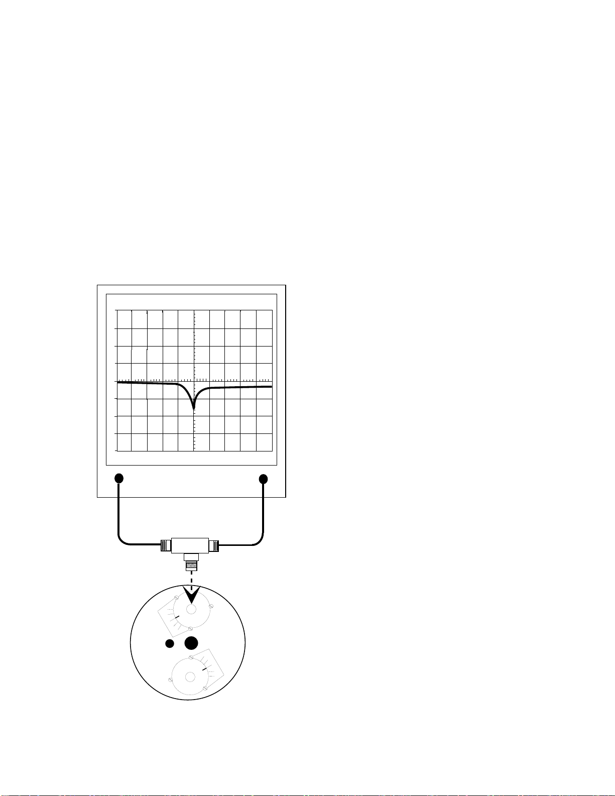
2. The resonant frequency of the filter is checked
by connecting the tracking generator to the input of the cavity filter while the spectrum analyzer is connected to the output, as shown in
figure 3.
50
dB
KHZ / DIV
8
6
4
2
0
-2
-4
-6
-8
dB
40
ANALYZER
98.00
MHZ
ATT
Used to determine 0 dB reference.
BANDPASS
FILTER
GEN
dBM
0
FEMALE UNION
20
15
10
5
0
20
15
10
5
0
Figure 3: Checking cavity tuning.
300
KHZ RES
MSEC
10
GENERATE
3. Insure the IFR A-7550 menu's are set as follows: DISPLAY - line
MODE - live
FILTER - none
SETUP - 50 ohm/dBm/gen1.
4. Set the fine tuning knob at it's mid-point. Adjust
the pass frequency by setting the peak (minimum loss value) of the response curve to the
desired frequency (should be the center-vertical
graticule line on the IFR A-7550's display). See
figure 3. The resonant frequency is adjusted by
using the coarse tuning rod, which is a sliding
adjustment (invar rod) that rapidly tunes the filter's response curve. The resonant frequency is
increased by pulling the rod out of the cavity
and is decreased by pushing the rod into the
cavity. Additionally, the fine tuning rod, also a
sliding adjustment (silver-plated-brass rod ), allows a more precise setting of the response
curve after the coarse adjustment is made. The
resonant frequency is increased by pushing the
fine tuning rod in and is decreased by pulling it
out, the exact opposite of the coarse tuning rod.
5. Once the desired response is obtained using
the coarse and fine tuning rods, they are
"locked" in place. The coarse rod is secured by
tightening the 10-32 cap screw and the fine
tuning rod is held in place by tightening the
knurled thumb nut. Failure to lock the tuning
rods will cause a loss of temperature compensation and detuning of the cavity.
Cavity Tuning Tip
When tuning a cavity that has been in service for
some time it is not unusual to find the main tuning
rod hard to move in or out. This occurs because
TX RX Systems Inc. uses construction techniques
borrowed from microwave technology that provide
large area contact surfaces on our tuning probes.
These silver plated surfaces actually form a
pressure weld that maintains excellent conductivity.
The pressure weld develops over time and must be
broken in order for the main tuning rod to move.
This is easily accomplished by gently tapping the
tuning rod with a plastic screwdriver handle or
small hammer so it moves into the cavity. The
pressure weld will be broken with no damage to the
cavity.
Measuring and Adjusting Insertion Loss
1. A zero reference must first be established at the
IFR A-7550 before the insertion loss can be
measured. This is accomplished by temporarily
placing a "female union" between the generator
output and analyzer input, see figure 3.
2. The flat line across the screen is the generator's
output with no attenuation, this value will become our reference by selecting the "Mode"
main menu item and choosing the "Store"
command.
3. Next select the "Display" main menu item and
choose the "Reference" command. This will
TX RX Systems Inc. Manual 7-9145-1 08/05/96 Page 3
Page 8

cause the stored value to be displayed on the
screen as the 0 dB reference
value.
4. Connect the generator output and analyzer input to the input/output ports of the loop plates
and the insertion loss will be displayed on the
IFR A-7550's screen, refer to figure 3.
5. Insertion loss is usually factory adjusted, at
which time index labels are attached to the top
of the cavity next to the loop plates and calibration marks are stamped into the loop plates
themselves. The index label serves as a relative
index with insertion loss settings keyed to index
numbers on the label. The calibration mark is
normally factory aligned so that the index value
of 10 will be equal to an insertion loss of 1.0 dB.
The relative index labels are used to log specific
filter performance. Insertion loss can be adjusted by loosening the 10-32 hold down screws
and rotating the loop plates.
6. Rotating the loop plate assemblies and moving
the calibration marks above or below 10 causes
the insertion loss to be increased or decreased
(above 10 increases the loss while below 10
decreases it). The insertion loss is adjustable
across a useable range of from 0.5 dB to 3.0
dB. It is important to set both loops to the
same index number so that the cavity's insertion loss remains balanced.
7. The insertion loss setting determines the selectivity of the filter and a change of loss will cause
a shift in the width of the passband. The pass
frequency of the cavity must be retuned after
the insertion loss is adjusted, as changes in
coupling also change the cavity's resonant frequency. Repeat steps 4 and 5 of the cavity tuning procedure in order to complete the cavity's
tuning.
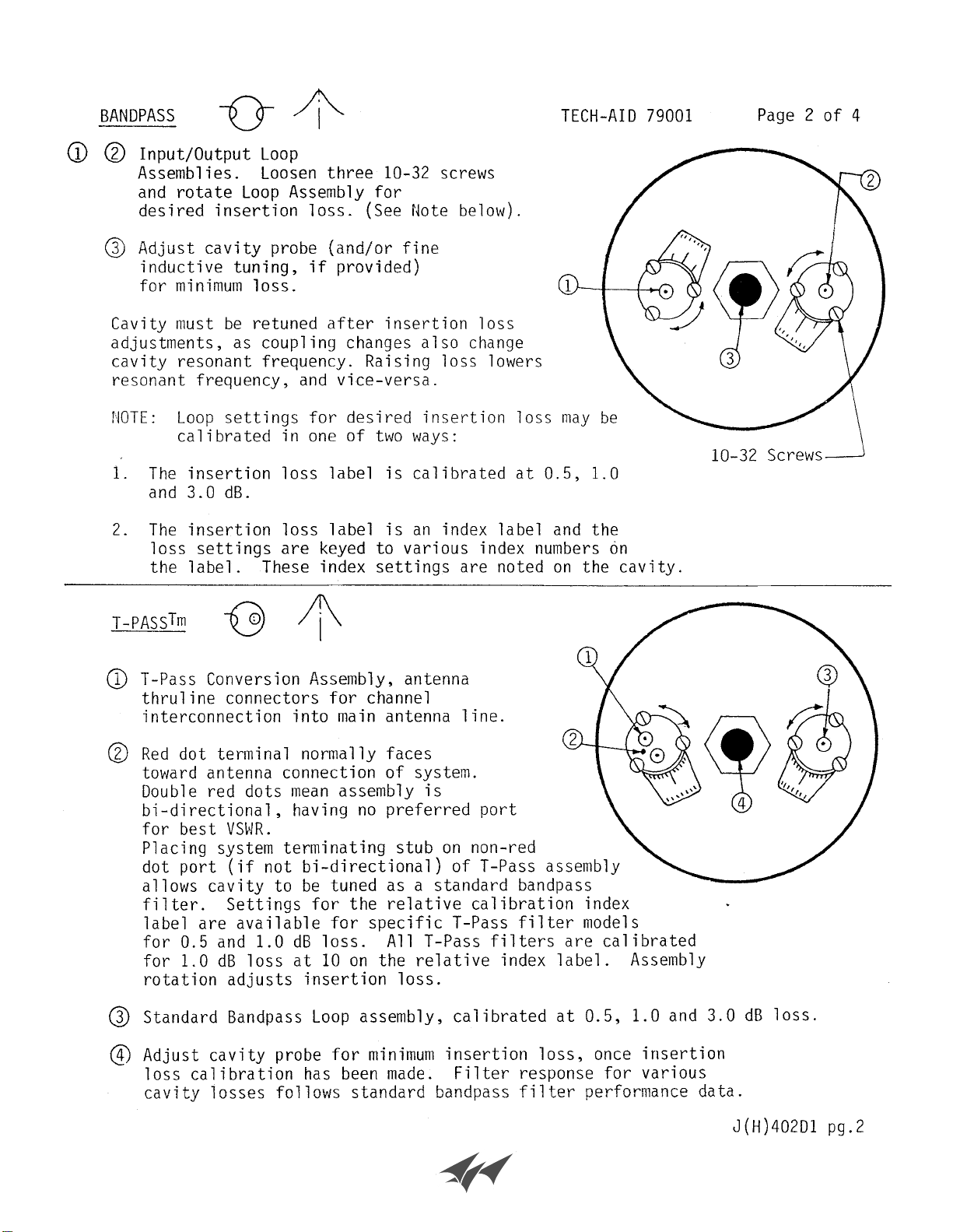
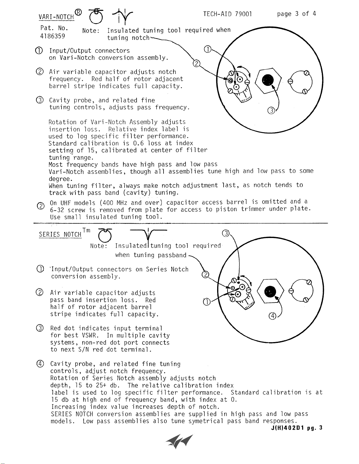
CONVERTING CAVITY RESONANT FILTERS
TX RX Systems Inc. produces four types of cavity
filters, including the Vari-Notch®, Series-Notch®,
Bandpass, and T-Pass®. The cavity resonator shell
along with the coarse and fine tuning controls are
standard subassemblies found in each type of filter
for a specified frequency band. Differences
between the types are determined by the loop plate
assemblies installed in the filter.
Bandpass
Filter Part #
11-28-01
11-28-05
11-29-01
11-29-05
11-35-01
11-35-05
11-36-01
11-36-05
11-37-01
11-37-05
11-54-01
11-54-05
11-55-01
11-55-05
11-65-01/-11
11-65-05/-25
11-69-01/-11
11-69-05/-25
11-70-01/-11
11-70-05/-25
Note: The last two digits of the filters model number indicate it's diameter and wavelength as listed below;
1.) Last digit of "01" indicates 6-5/8" diameter and 1/4 λ. 2.) Last digit of "11" indicates 6-5/8" diameter and 3/4 λ.
3.) Last digit of "05" indicates 10" diameter and 1/4 λ. 4.) Last digit of "25" indicates 10" diameter and 3/4 λ.
Vari-Notch
Lowpass Conversion
Kit Part #
76-28-02 76-28-03 76-28-04 76-28-05 76-28-07
76-29-02 76-29-03 76-29-04 76-29-05 76-29-07
76-35-02 76-35-03 76-35-04 76-35-05 76-35-07
76-36-03 76-36-04 76-36-05 76-36-06 76-38-01
76-37-03 76-37-04 76-37-05 76-37-06 76-38-01
N/A N/A N/A N/A 76-53-01
N/A N/A N/A N/A 76-53-01
76-65-03 76-65-04 76-65-05 76-67-01
76-69-03 76-69-04 76-69-05 76-67-01
76-70-03 76-70-04 7670-05 76-67-01
Vari-Notch
Highpass
Conversion
Kit Part #
Series-Notch
Lowpass
Conversion
Kit Part #
Series-Notch
Highpass
Conversion
Kit Part #
T-Pass
Conversion
Kit Part #
Table 2: Conversion kit part numbers.
TX RX Systems Inc. Manual 7-9145-1 08/05/96 Page 4
Page 9
The filter's loop plate assembly may be changed in
order to convert the cavity from one type of filter to
another. Conversion kits can be ordered which
contain all required parts for the conversion. The
available conversion kits are listed by part number
in table 2. Refer to the appropriate TX RX Systems
Inc. manual for the specific filter type once the kit is
installed.
Converting to Bandpass
When converting a Series-Notch or Vari-Notch filter
into a Bandpass filter an additional index label must
be applied to the cavity. Follow the procedure listed
below for correct placement.
2. The bandpass loop plate installed at the position of the existing index label should be rotated
until it's calibration mark aligns with the index
value of 10 and then tightened down into place
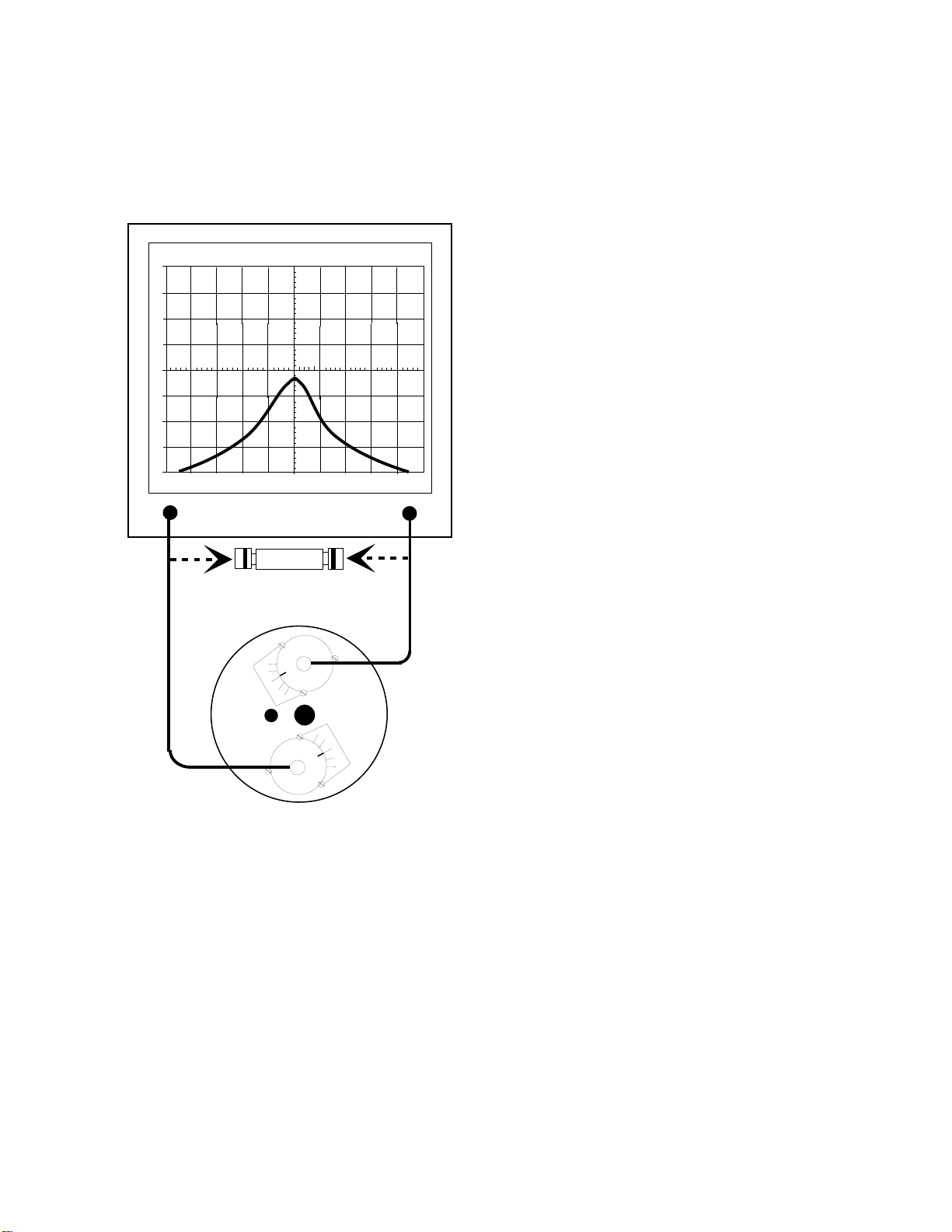
3. Measure its rejection notch as shown in figure 4
and record the value for comparison with the
unlabeled port. The amplitude of the rejection
notch is directly proportional to the insertion
loss .
4. Connect the tee to the remaining loop plate and
rotate it until its rejection notch is equal in value,
then tighten it down into place.
1. Install the bandpass loop plates into the loop
plates holes of the cavity.
1
dB
MHZ / DIV
40
30
20
10
0
-10
-20
-30
-40
dB
40
ANALYZER
98.00
MHZ
ATT
GEN
dBM
0
TEE CONNECTOR
Attach "UG-107 tee connector"
directly to the input / output port
300
KHZ RES
MSEC
10
GENERATE
5. Apply the second index label so that the value
of 10 lines up with the calibration mark.
6. Tighten all loop hold down screws.
When converting from a T-Pass filter into a
Bandpass the six steps listed above will not be
necessary. The T-Pass filter already has two
properly affixed index labels.
MULTIPLE CAVITY BANDPASS FILTERS
Bandpass filters can be ordered in multiple cavity
arrangements of either two or three combined
cavities. The filters are connected in a cascaded
fashion with the output of each filter fed to the input
port of the succeeding filter. The advantage of this
is that the amount of attenuation provided by each
of the filters is additive.
The interconnecting cable between the two filters,
when cut to the correct length (odd multiple of 1/4
λ), will provide up to 6 dB of additional attenuation
due to a mismatch of impedance between the
cable and the filters. The 6 dB of mismatch
attenuation does not occur at the filters passband
but, only at frequencies where moderate to high
attenuation occurs.
BANDPASS
FILTER
20
15
10
5
0
Because each of the filters in the multi-cavity
arrangement are identical, the passband for the
entire arrangement is generally the same as the
passband for the individual filters. However, each
0
5
10
15
20
filters individual insertion loss is also additive.
When tuning a multi-cavity arrangement, each filter
is tuned individually prior to interconnecting them.
Then each is fine tuned to peak the overall
response of the multi-cavity arrangement.
Figure 4: Measuring the rejection notch.
TX RX Systems Inc. Manual 7-9145-1 08/05/96 Page 5
Page 10
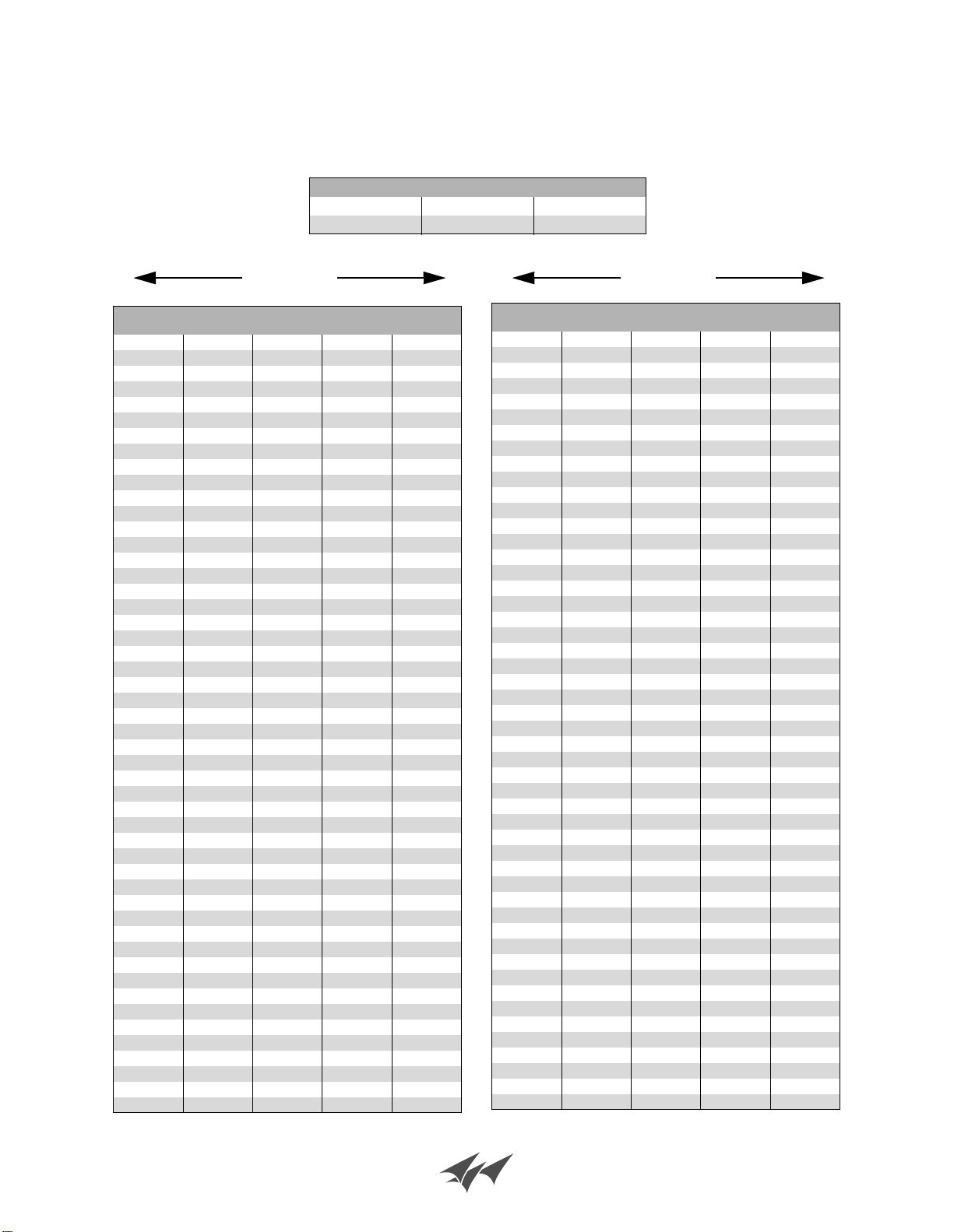
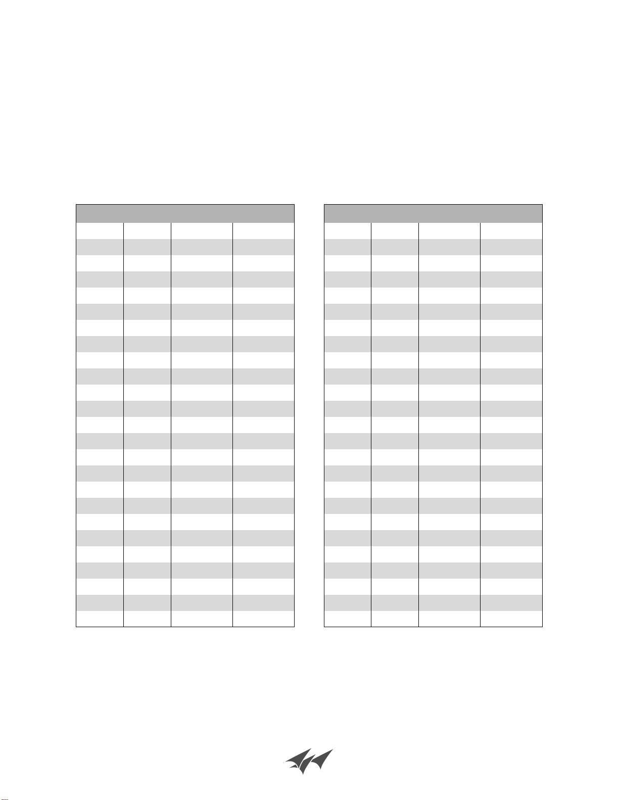
Power Ratio and Voltage Ratio to Decibel
Conversion Chart
Loss or Gain Power Ratio Voltage Ratio
+9.1 dB 8.128 2.851
-9.1 dB 0.123 0.351
- dB +- dB +
Voltage
Ratio
1 1 0 1 1
0.989 0.977 0.1 1.012 1.023
0.977 0.955 0.2 1.023 1.047
0.966 0.933 0.3 1.035 1.072
0.955 0.912 0.4 1.047 1.096
0.944 0.891 0.5 1.059 1.122
0.933 0.871 0.6 1.072 1.148
0.923 0.851 0.7 1.084 1.175
0.912 0.832 0.8 1.096 1.202
0.902 0.813 0.9 1.109 1.23
0.891 0.794 1 1.122 1.259
0.881 0.776 1.1 1.135 1.288
0.871 0.759 1.2 1.148 1.318
0.861 0.741 1.3 1.161 1.349
0.851 0.724 1.4 1.175 1.38
0.841 0.708 1.5 1.189 1.413
0.832 0.692 1.6 1.202 1.445
0.822 0.676 1.7 1.216 1.479
0.813 0.661 1.8 1.23 1.514
0.804 0.646 1.9 1.245 1.549
0.794 0.631 2 1.259 1.585
0.785 0.617 2.1 1.274 1.622
0.776 0.603 2.2 1.288 1.66
0.767 0.589 2.3 1.303 1.698
0.759 0.575 2.4 1.318 1.738
0.75 0.562 2.5 1.334 1.778
0.741 0.55 2.6 1.349 1.82
0.733 0.537 2.7 1.365 1.862
0.724 0.525 2.8 1.38 1.905
0.716 0.513 2.9 1.396 1.95
0.708 0.501 3 1.413 1.995
0.7 0.49 3.1 1.429 2.042
0.692 0.479 3.2 1.445 2.089
0.684 0.468 3.3 1.462 2.138
0.676 0.457 3.4 1.479 2.188
0.668 0.447 3.5 1.496 2.239
0.661 0.437 3.6 1.514 2.291
0.653 0.427 3.7 1.531 2.344
0.646 0.417 3.8 1.549 2.399
0.638 0.407 3.9 1.567 2.455
0.631 0.398 4 1.585 2.512
0.624 0.389 4.1 1.603 2.57
0.617 0.38 4.2 1.622 2.63
0.61 0.372 4.3 1.641 2.692
0.603 0.363 4.4 1.66 2.754
0.596 0.355 4.5 1.679 2.818
0.589 0.347 4.6 1.698 2.884
0.582 0.339 4.7 1.718 2.951
0.575 0.331 4.8 1.738 3.02
0.569 0.324 4.9 1.758 3.09
Power
Ratio
dB
Voltage
Ratio
Power
Ratio
Voltage
Ratio
0.562 0.316 5 1.778 3.162
0.556 0.309 5.1 1.799 3.236
0.55 0.302 5.2 1.82 3.311
0.543 0.295 5.3 1.841 3.388
0.537 0.288 5.4 1.862 3.467
0.531 0.282 5.5 1.884 3.548
0.525 0.275 5.6 1.905 3.631
0.519 0.269 5.7 1.928 3.715
0.513 0.263 5.8 1.95 3.802
0.507 0.257 5.9 1.972 3.89
0.501 0.251 6 1.995 3.981
0.496 0.246 6.1 2.018 4.074
0.49 0.24 6.2 2.042 4.169
0.484 0.234 6.3 2.065 4.266
0.479 0.229 6.4 2.089 4.365
0.473 0.224 6.5 2.113 4.467
0.468 0.219 6.6 2.138 4.571
0.462 0.214 6.7 2.163 4.677
0.457 0.209 6.8 2.188 4.786
0.452 0.204 6.9 2.213 4.898
0.447 0.2 7 2.239 5.012
0.442 0.195 7.1 2.265 5.129
0.437 0.191 7.2 2.291 5.248
0.432 0.186 7.3 2.317 5.37
0.427 0.182 7.4 2.344 5.495
0.422 0.178 7.5 2.371 5.623
0.417 0.174 7.6 2.399 5.754
0.412 0.17 7.7 2.427 5.888
0.407 0.166 7.8 2.455 6.026
0.403 0.162 7.9 2.483 6.166
0.398 0.159 8 2.512 6.31
0.394 0.155 8.1 2.541 6.457
0.389 0.151 8.2 2.57 6.607
0.385 0.148 8.3 2.6 6.761
0.38 0.145 8.4 2.63 6.918
0.376 0.141 8.5 2.661 7.079
0.372 0.138 8.6 2.692 7.244
0.367 0.135 8.7 2.723 7.413
0.363 0.132 8.8 2.754 7.586
0.359 0.129 8.9 2.786 7.762
0.355 0.126 9 2.818 7.943
0.351 0.123 9.1 2.851 8.128
0.347 0.12 9.2 2.884 8.318
0.343 0.118 9.3 2.917 8.511
0.339 0.115 9.4 2.951 8.71
0.335 0.112 9.5 2.985 8.913
0.331 0.11 9.6 3.02 9.12
0.327 0.107 9.7 3.055 9.333
0.324 0.105 9.8 3.09 9.55
0.32 0.102 9.9 3.126 9.772
Power
Ratio
dB
Voltage
Ratio
Power
Ratio
Bird Technologies Group TX RX Systems Inc.
Page 11
Bird Technologies Group TX RX Systems Inc.
Page 12
Bird Technologies Group TX RX Systems Inc.
Page 13
Bird Technologies Group TX RX Systems Inc.
Page 14
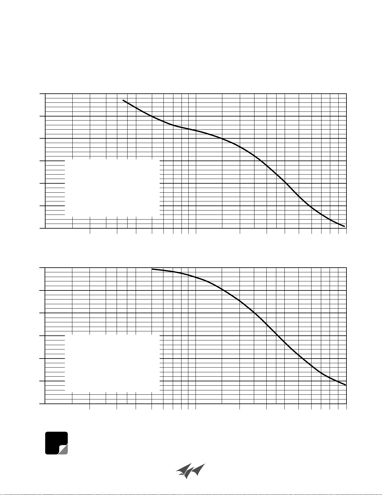
Isolation Curves for Transmitter/Receiver
The curves shown below for use with filters, duplexers, and multicouplers, indicate the
amount of isolation or attenuation required between a typical 100 watt transmitter and its
associated receiver at the TX (carrier suppression) and RX (noise suppression) frequency
which will result in no more than a 1 dB degradation of the 12 dB SINAD sensitivity.
100
90
80
70
Attenuation
60
50
40
100
132 - 174 MHz Band
For TX Power of:
25 watts -
50 watts 100 watts 250 watts 350 watts -
.2 .3 .4 .5 .6 .7 .8 .9 1 2 3 4 5 6 7 8 9 10
400 - 512 MHz Band
subtract 6 dB
subtract 3 dB
no correction
add 4 dB
add 5.5 dB
Frequency Separation (MHz)
90
80
70
Attenuation
60
50
40
NOTE
For TX Power of:
25 watts -
50 watts 100 watts 250 watts 350 watts -
.2 .3 .4 .5 .6 .7 .8 .9 1 2 3 4 5 6 7 8 9 10
These are only "typical" curves. When accuracy is required, consult the radio manufacturer.
subtract 6 dB
subtract 3 dB
no correction
add 4 dB
add 5.5 dB
Frequency Separation (MHz)
Bird Technologies Group TX RX Systems Inc.
Page 15
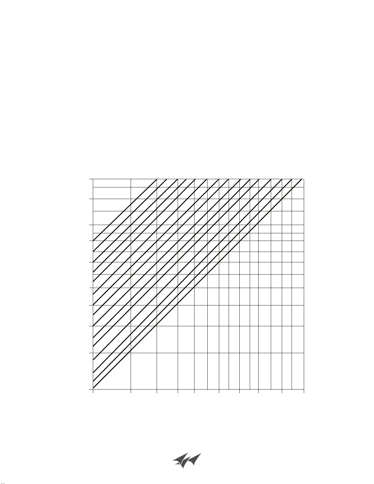
POWER IN/OUT
VS
INSERTION LOSS
The graph below offers a convenient means of determining the insertion loss of filters, duplexers,
multicouplers and related products. The graph on the back page will allow you to quickly determine
VSWR. It should be remembered that the field accuracy of wattmeter readings is subject to
considerable variance due to RF connector VSWR and basic wattmeter accuracy, particularly at low
end scale readings. However, allowing for these variances, these graphs should prove to be a useful
reference.
INSERTION LOSS (dB)
500
400
300
250
200
150
125
INPUT POWER (Watts)
100
7.0
6.5
6.0
5.5
5.0
4.5
4.0
3.5
3.0
2.5
2.0
1.5
1.0
.50
.25
75
50
50
75 100
125 150 200
250
300
400
500
OUTPUT POWER (Watts)
FOR LOWER POWER LEVELS
DIVIDE BOTH SCALES
BY 10 (5 TO 50 WATTS)
Bird Technologies Group TX RX Systems Inc.
Page 16
500
400
300
200
100
50
40
30
20
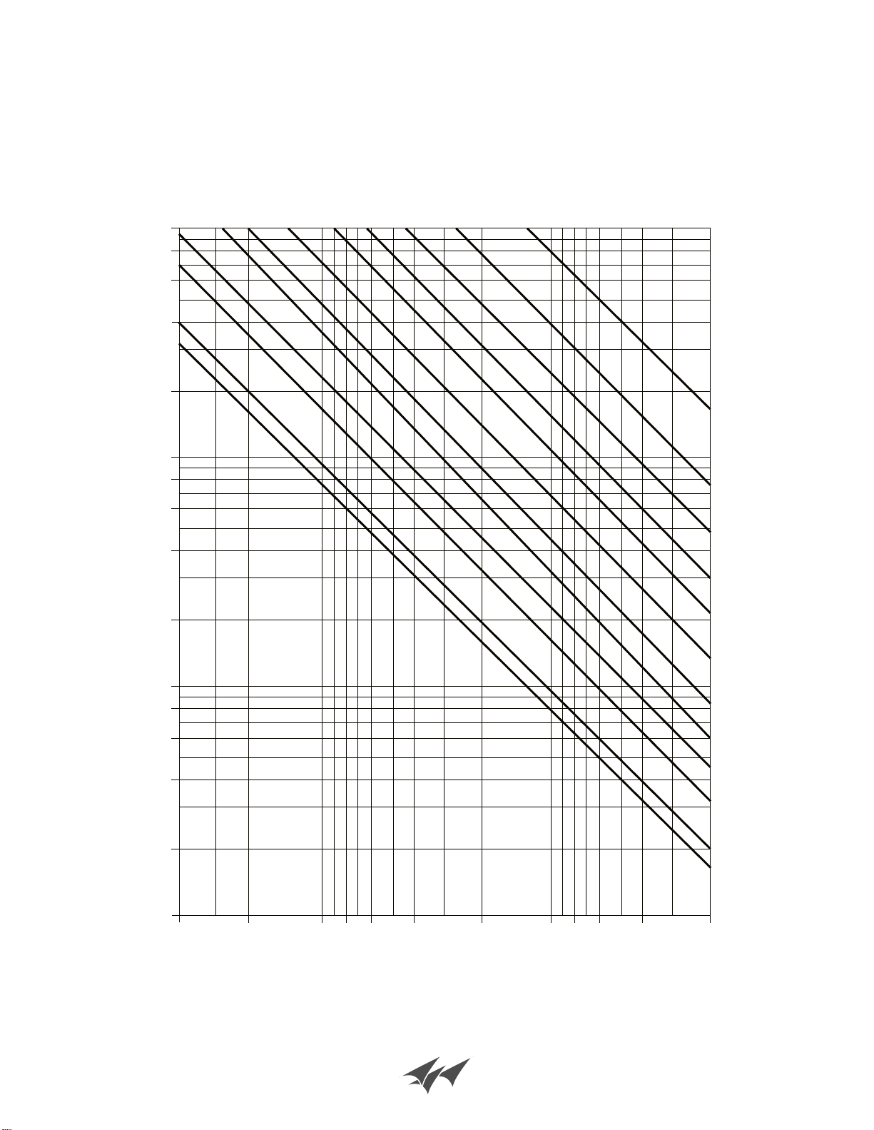
POWER FWD./REV.
VS
VSWR
V
S
W
R
1.1:1
1.15:1
1.2:1
10
FORWARD POWER (Watts)
5.0
4.0
3.0
2.0
1.0
0.5
40
20
10
8.0 6.0
4.0
2.0
REFLECTED POWER (Watts)
FOR OTHER POWER LEVELS
MULTIPLY BOTH SCALES
BY THE SAME MULTIPLIER
1.0 0.8
0.6
0.4
1.25:1
1.3:1
1.4:1
1.5:1
1.6:1
1.8:1
2.0:1
2.5:1
3.0:1
0.2
Bird Technologies Group TX RX Systems Inc.
Page 17
Power Conversion Chart
dBm to dBw to Watts to Volts
dBm dBw Watts
80 50 100kW 2236
75 45 31.6 kW 1257
70 40 10.0 kW 707
65 35 3.16 kW 398
60 30 1000 224
55 25 316 126
50 20 100 70.7
45 15 31.6 39.8
40 10 10.0 22.4
38 8 6.31 17.8
36 6 3.98 14.1
34 4 2.51 11.2
32 2 1.58 8.90
30 0 1.00 7.07
29 -1 0.79 6.30
28 -2 0.63 5.62
27 -3 0.50 5.01
26 -4 0.40 4.46
25 -5 0.32 3.98
24 -6 0.25 3.54
23 -7 0.20 3.16
22 -8 0.16 2.82
21 -9 0.13 2.51
20 -10 0.10 2.24
19 -11 79 mW 1.99
Volts 5 0 Ω
dBm dBw Watts
18 -12 63 mW 1.78
17 -13 50 mW 1.58
16 -14 40 mW 1.41
15 -15 32 mW 1.26
14 -16 25 mW 1.12
13 -17 20 mW 1.00
12 -18 16 mW 0.890
11 -19 13 mW 0.793
10 -20 10 mW 0.707
9 -21 7.9 mW 0.630
8 -22 6.3 mW 0.562
7 -23 5.0 mW 0.501
6 -24 4.0 mW 0.446
5 -25 3.2 mW 0.398
4 -26 2.5 mW 0.354
3 -27 2.0 mW 0.316
2 -28 1.6 mW 0.282
1 -29 1.3 mW 0.251
0 -30 1.0 mW 0.224
-5 -35 316 uW 0.126
-10 -40 100 uW 0.071
-15 -45 31.6 uW 0.040
-20 -50 10 uW 0.022
-25 -55 3.16 uW 0.013
-30 -60 1 uW 0.007
Volts 50Ω
Bird Technologies Group TX RX Systems Inc.
Page 18
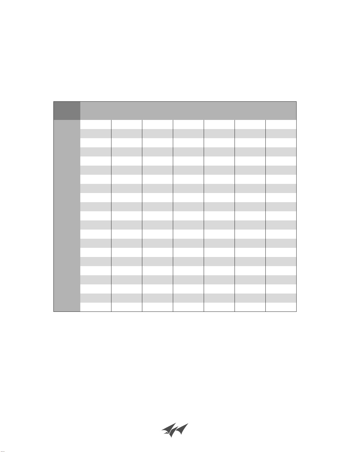
Free Space Path Loss Estimator
Frequency in MHz
50 150 170 450 500 800 900
0.1 50.58 60.12 61.21 69.66 70.58 74.66 75.68
0.25 58.54 68.08 69.17 77.62 78.54 82.62 83.64
0.5 64.56 74.10 75.19 83.64 84.56 88.64 89.66
1 70.58 80.12 81.21 89.66 90.58 94.66 95.68
2 76.60 86.14 87.23 95.68 96.60 100.68 101.71
3 80.12 89.66 90.75 99.21 100.12 104.20 105.23
4 82.62 92.16 93.25 101.71 102.62 106.70 107.73
5 84.56 94.10 95.19 103.64 104.56 108.64 109.66
6 86.14 95.68 96.77 105.23 106.14 110.22 111.25
7 87.48 97.02 98.11 106.57 107.48 111.56 112.59
8 88.64 98.18 99.27 107.73 108.64 112.72 113.75
9 89.66 99.21 100.29 108.75 109.66 113.75 114.77
10 90.58 100.12 101.21 109.66 110.58 114.66 115.68
Path Length (miles)
12 92.16 101.71 102.79 111.25 112.16 116.25 117.27
14 93.50 103.04 104.13 112.59 113.50 117.58 118.61
16 94.66 104.20 105.29 113.75 114.66 118.74 119.77
18 95.68 105.23 106.31 114.77 115.68 119.77 120.79
20 96.60 106.14 107.23 115.68 116.60 120.68 121.71
30 100.12 109.66 110.75 119.21 120.12 124.20 125.23
40 102.62 112.16 113.25 121.71 122.62 126.70 127.73
50 104.56 114.10 115.19 123.64 124.56 128.64 129.66
Formula: Path Loss (dB) = 36.6 + 20 log (MHz) + 20 log (miles)
Bird Technologies Group TX RX Systems Inc.
Page 19
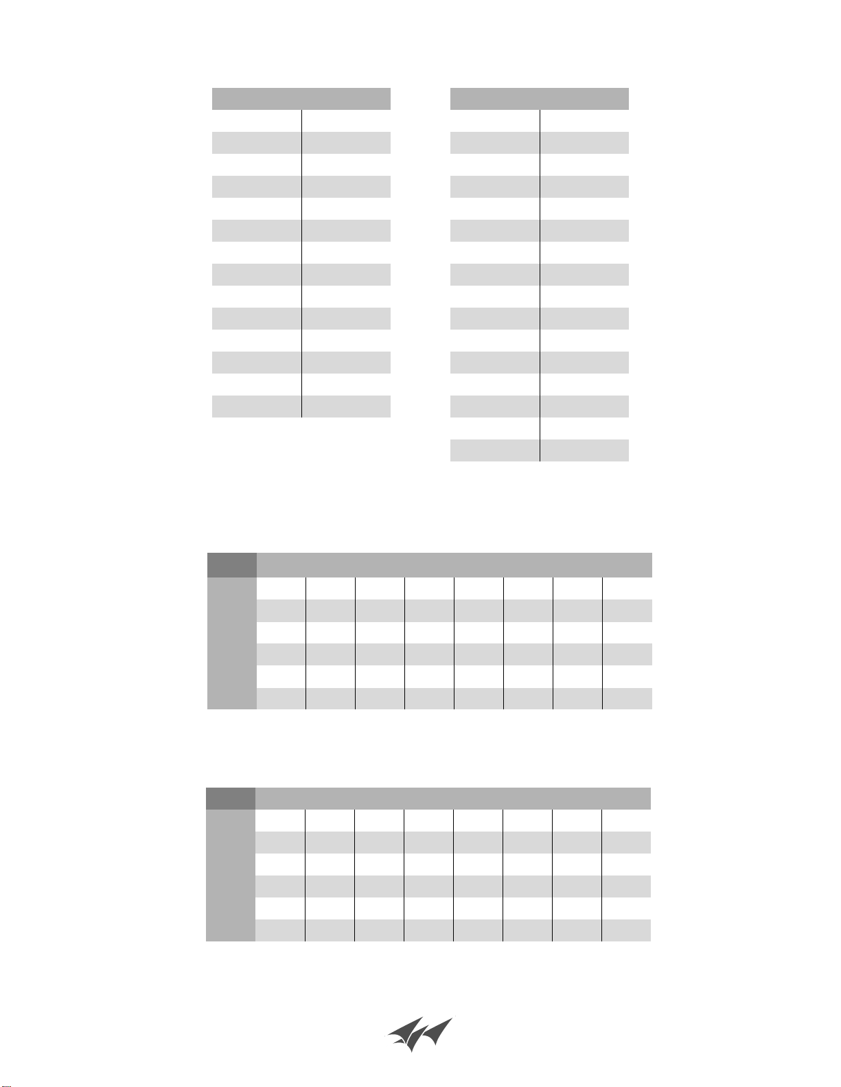
Return Loss vs. VSWR
Watts to dBm
Return Loss VSWR
30 1.06
25 1.11
20 1.20
19 1.25
18 1.28
17 1.33
16 1.37
15 1.43
14 1.50
13 1.57
12 1.67
11 1.78
10 1.92
9 2.10
Watts dBm
300 54.8
250 54.0
200 53.0
150 51.8
100 50.0
75 48.8
50 47.0
25 44.0
20 43.0
15 41.8
10 40.0
5 37.0
4 36.0
3 34.8
2 33.0
1 30.0
dBm = 10log P/1mW
Where P = power (Watt)
Insertion Loss
Input Power (Watts)
50 75 100 125 150 200 250 300
3 25 38 50 63 75 100 125 150
2.5 28 42 56 70 84 112 141 169
2 32 47 63 79 95 126 158 189
1.5 35 53 71 88 106 142 177 212
1 40 60 79 99 119 159 199 238
Insertion Loss
.5 45 67 89 111 134 178 223 267
Output Power (Watts)
Free Space Loss
Distance (miles)
.25 .50 .75 1 2 5 10 15
150 68 74 78 80 86 94 100 104
220 71 77 81 83 89 97 103 107
460 78 84 87 90 96 104 110 113
860 83 89 93 95 101 109 115 119
940 84 90 94 96 102 110 116 120
Frequency (MHz)
1920 90 96 100 102 108 116 122 126
Free Space Loss (dB)
Free space loss = 36.6 + 20log D + 20log F
Where D = distance in miles and F = frequency in MHz
Bird Technologies Group TX RX Systems Inc.
Page 20

8625 Industrial Parkway, Angola, NY 14006 Tel: 716-549-4700 Fax: 716-549-4772 sales@birdrf.com www.bird-technologies.com
 Loading...