biochrom NanoVue Plus User Manual

Page 1

NanoVue Plus

™

Product User Manual

Biochrom US Telephone: 1-508-893-8999 84 October Hill Rd Toll Free: 1-800-272-2775 Holliston, MA Fax: 1-508-429-5732 01746-1388 support@hbiosci.com USA www.biochromspectros.com

Page 2

5061-049 REV 1.4

1. INSTALLATION 3

1.1. Unpacking and positioning 3

1.2. Safety 3 4

2. INTRODUCTION 5

2.1. Your NanoVue Plus 5

2.2. File system 6

2.3. Data export 6

2.4. Sample treatment 7

2.5. Pathlength and Absorbance nomalization 7

2.6. Auto-Read 8

2.7. Quality Assurance 8

2.8. Keypad and display 9

2.9. Software style 10

3. OPERATION AND MAINTENANCE 11

3.1. Sample application guide 11

3.2. Sample Plate replacement 12

3.3. Cleaning and general maintenance 13

3.4. Return for repair 13

3.5. Lamp replacement 13

3.6. Replacing the printer paper 13

4. LIFE SCIENCE 14

4.1. File system 14

4.2. Nucleic acids 14

4.2.1. Theory 14

4.2.2. DNA measurement 16

4.2.3. RNA measurement 17

4.2.4. Oligonucleotide measurement 19

4.2.5. T

Calculation 20

4.2.6. CyDye™ measurement 23

4.3. Proteins 26

4.3.1. Theory 26

4.3.2. Protein UV 28

4.3.3. Protein A280 30

4.3.4. BCA 31

4.3.5. Bradford 34

4.3.6. Lowry 36

4.3.7. Biuret 39

5. APPLICATIONS 42

5.1. File system 42

5.2. Single Wavelength 42

5.3. Concentration 44

5.4. Wavescan 46

5.5. Kinetics 48

5.6. Standard Curve 50

5.7. Multiple Wavelength 53

5.8. Absorbance Ratio 54

6. FAVOURITES AND METHODS 56

7. UTILITIES 57

7.1. Date and time 57

7.2. Regional 57

7.3. Printer 58

7.4. Preferences 58

7.5. Contrast 58

7.6. About 58

7.7. Pathlength Check & Calibration 59

7.8. Games 62

8. ACCESSORIES 63

8.1. Printer installation 63

8.2. Bluetooth accessory installation 65

8.3. Fitting SD memory card accessory 67

8.4. After sales support 70

9. TROUBLESHOOTING 71

9.1. Pathlength calibration over-range 71

9.2. Error messages 72

9.3. Fault analysis 74

9.4. Frequently asked questions 74

10. SPECIFICATION AND WARRANTY 77

11. LEGAL

Page finder

Page 3

5061-049 REV 1.4

1. INSTALLATION

1.1. Unpacking and positioning

• Removetheinstrumentfromitspackagingandinspectitforsignsofdamage.If

any are discovered, inform your supplier immediately.

• Theinstrumentmustbeplacedonastable,levelsurfacethatcantakeitsweight (~ 4.5 kg) and positioned such that air can circulate freely around the casing.

• Ensureyourproposedinstallationsiteconformstotheenvironmentalconditions

for safe operation.

• Theinstrumentisdesignedforindooruseonly,temperaturerange5°Cto35°C

and should be kept away from strong draughts.

• Ifyouusetheinstrumentinaroomsubjectedtoextremesoftemperature

change during the day, it may be necessary to recalibrate (by switching off and then on again) once thermal equilibrium has been established (2–3 hours).

• Atemperaturechangeofnomorethan4°C/hourandamaximumrelative humidityof80%at31°C,decreasinglinearlyto50%at40°Carerequired.

• Iftheinstrumenthasjustbeenunpackedorhasbeenstoredinacold

environment, it should be allowed to come to thermal equilibrium for 2–3 hours in the laboratory before switching on. This will prevent calibration failure as a result of internal condensation.

• Theinstrumentmustbeconnectedtothepowersupplywiththepoweradaptor

supplied. The adaptor can be used on 90–240V, 50–60Hz supplies. It will become warm once plugged into the power supply and should not be covered up.

• Switchontheinstrumentviathekeypad(

) after it has been plugged in. The

instrument will perform a series of self-diagnostic checks.

• Itisrecommendedthatusersreadthroughthismanualpriortouse.

• Contactyoursupplierifyouexperienceanydifficultieswiththisinstrument

• Werecommendthatyoucarryoutaquickcheckofthepathlengthbeforeusing

1.2. Safety

Spectrophotometer Health & Safety Document including General Operating Instructions are available as a booklet provided with each instrument. The booklet, translated into the European Union languages, is available on the delivered CD. The instructions provide the user with basic use, troubleshooting and how to use the instrument in a safe manner.

CAUTION

This instrument contains a UV source which generates a light beam that

is present at the sample platform. Do not attempt to divert the beam as prolonged exposure to the beam may cause permanent eye damage.

Note that the instrument prevents operation if the head is raised or the Xenon ﬂash does no reach the detection system.

the NanoVue, please see instructions on how to do this in section 7.7.

1. INSTALLATION

1.1. Unpacking and positioning

• Removetheinstrumentfromitspackagingandinspectitforsignsofdamage.If

any are discovered, inform your supplier immediately.

• Theinstrumentmustbeplacedonastable,levelsurfacethatcantakeitsweight (~ 4.5 kg) and positioned such that air can circulate freely around the casing.

• Ensureyourproposedinstallationsiteconformstotheenvironmentalconditions

for safe operation.

• Theinstrumentisdesignedforindooruseonly,temperaturerange5°Cto35°C

and should be kept away from strong draughts.

• Ifyouusetheinstrumentinaroomsubjectedtoextremesoftemperature

change during the day, it may be necessary to recalibrate (by switching off and then on again) once thermal equilibrium has been established (2–3 hours).

• Iftheinstrumenthasjustbeenunpackedorhasbeenstoredinacold

environment, it should be allowed to come to thermal equilibrium for 2–3 hours in the laboratory before switching on. This will prevent calibration failure as a result of internal condensation.

• Theinstrumentmustbeconnectedtothepowersupplywiththepoweradaptor

supplied. The adaptor can be used on 90–240V, 50–60Hz supplies. It will become warm once plugged into the power supply and should not be covered up.

• Switchontheinstrumentviathekeypad(

) after it has been plugged in. The

instrument will perform a series of self-diagnostic checks.

• Itisrecommendedthatusersreadthroughthismanualpriortouse.

• Contactyoursupplierifyouexperienceanydifficultieswiththisinstrument

• Werecommendthatyoucarryoutaquickcheckofthepathlengthbeforeusing

WARNING

High voltages exist inside the NanoVue Plus instruments. Repair and maintenance should only be carried out by individuals trained specifically to work on these instruments.

Page 4

5061-049 REV 1.4

If the instrument is used in a manner not speciﬁed or in environmental conditions not appropriate for safe operation, the protection provided may be impaired and instrument warranty withdrawn.

There are no user-serviceable parts inside this instrument.

Page 5

5061-049 REV 1.4

2. INTRODUCTION

2.1. Your NanoVue Plus

NanoVue Plus is a simple-to-use UV/Visible instrument with twin CCD array detectors (1024 pixels) and few moving parts, which contributes to its inherent reliability.

General Principles

In conventional UV/Visible spectrophotometers, the sample is usually contained within a glass or silica cuvette which is placed in the sample beam. The Absorbance of this is measured and then compared to that of a standard. From this comparison, the concentration is calculated.

However, when the quantity of sample is limited or highly concentrated, dilution or the use of ultra low volume cuvettes is required, which is time consuming, can introduce errors and presents cleaning difficulties.

NanoVue Plus was developed to overcome these problems. Using NanoVue Plus, typical sample volumes of 2 µl are pipetted onto a hydrophobic surface and then a very short pathlength of either 0.2 mm or 0.5 mm is created by lowering the sampling head onto the top of the sample.

With the sample so constrained, all of the general software features of the instrument, including wavelength scanning, single or multi-wavelength Absorbance and concentration measurement, kinetics, standard curves and Absorbance ratio, can be utilized. In all of these modes, the instrument utilizes either the 0.2 mm or 0.5 mm pathlengths. The benefit of these small pathlengths is that the instrument can measure smaller volumes of very concentrated or highly absorbing samples.

NanoVue Plus also has a range of more specific life science applications, including DNA and RNA concentration and purity, Oligonucleotide concentration, Tm Calculation, Cy Dye concentration and a variety of protein measurements. In all of these applications, instead of the actual Absorbance measurement being used, the value is normalized to reflect a standard pathlength of 10 mm, so that generally accepted factors (50 for DNA, 40 for RNA and 33 for oligos, for example) can be used to calculate concentration. As an example, if the absolute Absorbance of the sample is 0.025 A using a pathlength of 0.5 mm, the normalized Absorbance shown will be 0.500 A.

NanoVue Plus is therefore ideally suited to the life scientist where sample is limited and speed and convenience of analysis is key.

Figure 1: NanoVue Plus Spectrophotometer

UV-Visible

Page 6

5061-049 REV 1.4

2.2. File system

After switch on and automatic checking the instrument defaults to a home page entitled ‘NanoVue Plus‘. This page displays five folders which form the topmost layer of a simple file tree which is the basis of the user-interface. The folder screens are reached by pressing the appropriate number on the keypad, with return to the top level by means of the ‘Esc’ key. The folders group various facilities together as follows:-

1. Life Science Standard life science applications such as nucleic acid and protein assays.

2. Applications General spectroscopic applications.

3. A folder to store your more frequently used methods.

(Inactive when empty)

4. Methods Contains 9 folders that can store less frequently used methods. Up to 9 methods per folder are allowed, totalling 81 methods.

5. Utilities Instrument set up options and games.

Figure 2: NanoVue Plus with Printer

Favorites

Data can be transferred to a PC, either via a Bluetooth accessory (supplied preinstalled or as an optional accessory) or via a USB cable. The software to perform this task “PVC” (Print Via Computer) is a small application running under Windows 2000™, Windows XP™ or Windows 7, 8, 8.1. PVC can operate via USB and Bluetooth simultaneously.

PVC can store data either in a common directory or can be conﬁgured to save to independent directories by both ﬁle format and connection. The data may be stored as an Excel spreadsheet, an EMF graphics ﬁle, a comma delimited (csv) data ﬁle, a tab delimited (txt) data ﬁle, rich text format (RTF) which is compatible with Word or in native PVC format.

Some users may ﬁnd it convenient to “print through” the PC directly to a printer already attached to it. The software to enable this option will be found on the CD provided.

Datrys Computer control software is also available for NanoVue Plus as an optional extra.

2.3. Data export

An integral printer is available for the instrument; this may be either supplied pre-installed or as an optional accessory. The installation procedure is described in section 8.1.

(Games only available if selected via the Preferences Screen)

Page 7

5061-049 REV 1.4

2.4. Sample treatment

NanoVue Plus uses a unique sampling head which enables users to accurately measure the optical characteristics of samples volumes as low as 0.5 µl. The sample is applied to a horizontal plate having a hydrophobic surface, the sampling head is lowered into position and the reading taken. The pathlength is

automaticallyadjustedunlesstheuserselectsmanualadjustment.Thiscanbe

either 0.2 mm or 0.5 mm.

Application of the sample is most conveniently carried out using any commercially available pipetting tool and standard tips, a 10 µl pipette is recommended.

2.5. Pathlength and Absorbance normalization

For methods in the Application folder, the Absorbance values have not been normalized and the pathlength needs to be taken into account when the values are used for concentration calculations. NanoVue Plus has the ability to measure samples using either a 0.2 mm or a 0.5 mm pathlength. The 0.5 mm pathlength should be used for samples of low concentration and the 0.2 mm pathlength for more concentrated samples. It is best to use the 0.5 mm pathlength whenever possible. In the Life Science applications, the Absorbance readings are presented as their normalized 10 mm pathlength values, to allow the use of literature based factors for concentration measurements.

Within the DNA, RNA, Oligonucleotide, Tm Calculation, Cy Dye, Protein UV and Protein A280 methods the system defaults to having the pathlength chosen automatically. When this is active, the instrument will measure at the 0.5 mm pathlength first and if the Absorbance is high (> 1.7 A) then the measurement will be carried out at the 0.2 mm pathlength. If the concentration range of the samples is known beforehand, the relevant pathlength can be pre-selected; if it is unknown then the automatic option can be used. Within the other applications, the actual measured Absorbance value is reported, so if the Absorbance is high at the

0.5 mm pathlength (> 1.7 A), the sample can be re-measured at the 0.2 mm pathlength. In the automatic mode, the reference scan is always carried out using both pathlengths, so that if a sample is measured at one pathlength and subsequently re-measured at the other pathlength, a new reference scan is not required.

The pathlength that is used to carry out the measurement is printed/exported with each result and is also displayed in the top left hand corner of the header line on the instrument’s display. Care must be taken that the correct pathlength is being used when comparing sample results or using a stored calibration curve.

Figure 3a: Sample head

Figure 3b: Sample application

Page 8

5061-049 REV 1.4

2.6. Auto-Read

NanoVue Plus senses when the sampling head has been lowered, so Auto-Read can be used to automatically make a measurement when this happens, obviating the need to press any keys. The instrument assumes that the first reading after starting any application will be a reference scan and that subsequent readings will be sample scans.

Switching Auto-Read on or off:

Go to Utilities (option 5 from the NanoVue Plus menu). Select Preferences (option 4). Use the arrow keys to go to the Lid Switch option and select On to turn Auto-Read

on, or Off to turn Auto-Read off. Press the confirm button. When Auto-Read is off, use the 0A/100%T and

keys to take the reference and

measurement scans respectively. When Auto-Read is on, the keys on the keypad are still functional. This enables

a user to carry out a new reference scan at any time by pressing the 0A/100%T key prior to lowering the sampling head, or to perform a series of readings or reference scans without raising the sampling head.

2.7. Quality Assurance

Quality Assurance is provided to help minimize the impact of pipetting errors. If Quality Assurance is switched on from the Preferences Screen, the instrument will ask the user for a second reference to compare with the first to ensure that the reading is reasonable. If the second reading is not sufficiently close to the first reading, the user will be asked to replace the reference again. The process will be repeated until two successive good readings (within 0.02 A) are identified and the reference will be the average of these readings.

Note: When the user is prompted for the second reference, the user is required to clean the surface and reapply the sample. The 0A/100%T key is disabled until

theuserliftsthesamplingheadtopreventtheuserfromjustre-readingthesame

sample.

0.5 mm pathlength

0.2 mm pathlength

Page 9

5061-049 REV 1.4

Key Action

On/Off key Turns the instrument on/off.

Arrow keys Use the four arrow keys to navigate around

the display and select the required setting from the active (highlighted) option.

View options



View options for that application mode. Some of these are common to all applications and are described below. Options unique to an application are described in the relevant section.

Alphanumeric keys Use these to enter parameters and to write

text descriptions. Use repeated key presses to cycle through lower case, number and upper case. Leave for 1 second before entering the next character. Use the C key to backspace and the 1 key to enter a space.

Escape/Cancel

Esc

Escape from a selection and return to the previous folder.

Set Reference

100%T

Set reference to 0.000 A or 100%T on a reference solution at the current wavelength in the mode selected. When in scan mode, make a reference scan.

Confirm selection

Confirms a selection.

Take measurement

Makes a measurement.

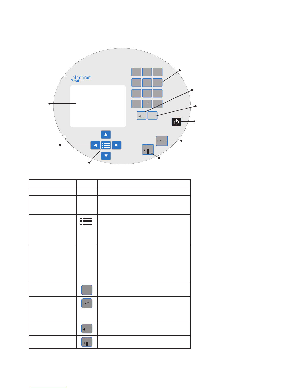
2.8. Keypad and display

The back-lit liquid crystal display is very easy to navigate around using the alphanumeric entry and arrow keys on the hard-wearing, spill-proof membrane keypad.

100%T

Esc

abc

def

mno

jkl

ghi

wxyz

tuv

pqrs

+ / -

T/U

100% T

Alphanumeric

Conﬁrm selection

Escape/Cancel

On/Off

Set reference

Take measurement

View options

Arrow keys

Display screen

Page 10

5061-049 REV 1.4

Options Sub Menu (select using keypad numbers)

1. View Parameters for the experiment.

2. Print the results. 3, 4, 5, 6 Described in the relevant application.

7. Define the Sample Number you wish to start from.

8. Save the parameters as a method to a defined folder name with

a defined method name.

9. Toggle Auto-Print on/off. Default is off.

Exit options by pressing Esc

Esc

or wait.

Experienced operators can use the numeric keys as a shortcut to the option required without needing to enter the Options menu.

2.9. Software style

The user interface is built around folders of files which are displayed on the first page when the instrument is switched on. Different folders are numbered and opened by using the associated number key on the keypad.

1. Standard life science applications such as nucleic acid and protein assays.

2. General spectroscopic applications.

3. A folder to store your more frequently used

methods. (Inactive when empty)

4. Contains 9 folders that can store less frequently used methods. Up to 9 methods per folder are allowed, totaling 81 methods.

5. Instrument set up options and games. (Games only available if selected via the

Preferences Screen)

Summary Function Keypad Number Description

Page 11

5061-049 REV 1.4

3. OPERATION AND MAINTENANCE

3.1. Sample application guide

Step 1

Lift the sampling head to the vertical position and using a low-volume (0–10 µl) pipette take up approximately 2 µl of sample. A reliable pipette and matching high quality tips are strongly recommended.

When removing a very small aliquot from a larger volume, ensure that the sample is truly representative. Filtration may also be advantageous.

Step 2

Carefully apply the sample so that it sits over the black spot between the four alignment spots, (see Figure: 4).

Take care not to introduce bubbles into the sample.

After the plunger is depressed, lift the pipette up carefully so as not to drag the droplet off-target.

Step 3

Observe the position and shape of the drop; it should resemble the one shown in Figure: 6a rather than 6b. A noticeably spread-out sample indicates the target area may be contaminated and requires cleaning (see below). Gently lower the sampling head.

Figure 4

Figure 5

Figure 6a

Figure 6b

Return light path

Page 12

5061-049 REV 1.4

Step 4

If a program has been selected and the Auto-Read function is set to On (see section 2.6), the sample reading process will begin automatically – a reference scan will be taken first, followed by the measurement scan.

If the Auto-Read function is set to Off, use the 0A/100%T and

buttons to take the reference and measurement scans respectively. Note: It is not recommended to raise and lower the head repeatedly to take multiple measurements of one sample, this can cause the droplet to disperse. If repeat measurements are required use the button

Step 5

If you wish to keep the sample it can be recovered after the reading has been taken using a pipette.

Step 6

After taking the reading, both the top and bottom plates should be cleaned by wiping away the sample using a soft lint-free tissue. Wipe the bottom plate towards you and the top plate upwards to avoid contaminating the return light path to the rear (see previous figure 6a).

It may be necessary to remove sticky or dried-on residues. Water or a dilute (2%) detergent solution should suffice. After using detergent, the plates should be wiped a second time with either water or Isopropanol (2-propanol).

3.2. Sample Plate replacement

If after careful cleaning the droplet shape is still unsatisfactory, or if either of the plates becomes damaged, or there is deterioration of the hydrophobic coating, then it will be necessary to replace them as a pair. The glass plates are permanently fixed within plastic housings which clip to the sample handling module. Replacements are available from your supplier.

Exchanging the sample plates is simple (see Figures: 8a and 8b). They are available from your supplier under part number 28-9244-06

1. Remove the top sample plate. Put one thumb at the base of the sample plate

and with the other hand gently lever down the tab at the top of the plate.

2. Replace the top sample plate. Insert the bottom tab and hold this in place with

one thumb and then gently push the tab at the top until the plate clicks into place. Once in position, two silver pins will be visible either side of the top sensor.

3. Remove the bottom sample plate. Gently lever the plate upwards using the

thumb tab at the front of the plate and then pull it towards you to remove it completely.

4. Replace the bottom sample plate. Gently insert the tabs at the back of the plate

as far as they will go and then push down the front of the sample plate so the tabs underneath are fully pushed in.

5. Always calibrate the system after replacing the sample plates.

Figure: 7a

28955301.

Locate the screw above the bottom sample plate. Turn counter clockwise to loosen. Remove the bottom sample plate. Gently lever the plate upwards using the thumb tab at the front of the plate and then pull it towards you to remove it completely.

Replace the bottom sample plate. Gently insert the tabs at the back of the plate as far as they will go and then push down the front of the sample plate so the tabs underneath are fully pushed in. Insert screw back in, turn clockwise to tighten.

Page 13

5061-049 REV 1.4

3.3. Cleaning and general maintenance

Before cleaning the case of the instrument, switch off the instrument and disconnect the power cord.

Clean all external surfaces using a soft damp cloth. A mild liquid detergent may be used to remove stubborn marks.

3.4. Return for repair

The responsibility for decontamination of the instrument lies with the customer. The case may be cleaned with mild detergent or an alcohol such as ethanol or Isopropanol.

Examination or repair of returned instruments cannot be undertaken unless they are accompanied by a decontamination certificate signed by a responsible person.

Figure: 8a

Figure: 8b

3.3. Cleaning and general maintenance

Before cleaning the case of the instrument, switch off the instrument and disconnect the power cord.

Clean all external surfaces using a soft damp cloth. A mild liquid detergent may be used to remove stubborn marks.

3.4. Return for repair

The responsibility for decontamination of the instrument lies with the customer. The case may be cleaned with mild detergent or an alcohol such as ethanol or Isopropanol.

Examination or repair of returned instruments cannot be undertaken unless they are accompanied by a decontamination certificate signed by a responsible person.

This could be of the following form:-

3.5. Lamp replacement

The xenon lamp should not need replacement until used for several years. In the unlikely event that it does fail, this should be undertaken by a service engineer from your supplier.

3.6. Replacing the printer paper

Spare paper for the printer (20 rolls) is available from your supplier under part

number 28918226

Step 1 Keep the power on. Lift off the paper cover. Step 2 Lock the platen (horizontal position) and feed the paper into the slot.

The drive will engage automatically and take up the paper.

Step 3 It may help to release the platen lock (turn flat green catch clockwise) and

turn the green knob manually.

Step 4 Replace the cover.

Figure: 8a

Figure: 8b

Please contact technical support at support@hbiosci.com for assistance.

Page 14

5061-049 REV 1.4

4. LIFE SCIENCE

4.1. File system

The Life Science Screen is organized into six sub-folders as shown below:

Folder Keypad Number Application Function

1 DNA Concentration and purity check for DNA samples 2 RNA Concentration and purity check for RNA samples 3 Oligo Concentration and purity check for Oligonucleotide samples 4 Tm Calculation DNA melting point calculator 5 Cy Dye Labeling efﬁciency measurement 6 Protein Folder containing methods for protein determination

Pressing 6 enters the Protein sub-folder which contains various standard methods for protein determination:-

4.2. Nucleic Acids

4.2.1. Theory

•Nucleicacidscanbequantifiedat260nmbecauseatthiswavelengththere

is a clearly defined peak maximum. A 50 µg/ml DNA solution, a 40 µg/ml RNA solution and 33 µg/ml solution of a typical synthetic Oligonucleotide all have an optical density of 1.0 A in a 10 mm pathlength cell. These factors (50, 40 and 33 respectively) can be inserted into the formula (1) below, although they do vary with base composition and this can be calculated more precisely if the base sequence is known.

(1) Concentration = Abs260 * Factor (where * means “multiplied by”)

Page 15

5061-049 REV 1.4

•NanoVuePluswilldefaulttofactors50fordoublestrandedDNA,40forRNA

and 33 for single stranded DNA and Oligonucleotides. It also allows manual compensation for dilution - aided by a dilution calculator.

•Nucleicacidsextractedfromcellsareaccompaniedbyproteinandextensive

purification is required to remove the protein impurity. The 260/280 nm Absorbance ratio gives an indication of purity, however it is only an indication and not a definitive assessment. Pure DNA and RNA preparations have expected ratios of 1.7–1.9 and ≥ 2.0 respectively. Deviations from this indicate the presence of impurity in the sample, but care must be taken in the interpretation of results.

•The260nmreadingistakennearthetopofabroadpeakintheAbsorbance

spectrum for nucleic acids, whereas the 280 nm reading naturally occurs on a steep slope, where small changes in wavelength will result in large changes in Absorbance. Consequently, small variations in wavelength accuracy have a much larger effect at 280 nm than at 260 nm. It follows therefore that the 260/280 ratio is susceptible to this effect and users are warned that spectrophotometers of different designs may give slightly different ratios.

•Inpractice,concentrationalsoaffectsthe260/280ratioastheindividual

readings approach the instrument’s detection limit. If a solution is too dilute, the 280nm reading shows a greater proportional interference from background and as the divisor becomes smaller, has a disproportionate effect on the final result.

It is advisable to ensure that the Abs260 value is greater than 0.1 A for accurate measurements.

•AnelevatedAbsorbanceat230nmcanalsoindicatethepresenceofimpurities.

230 nm is near the Absorbance maximum of peptide bonds and may also indicate interference from common buffers such as Tris and EDTA. When measuring RNA samples, the 260/230 ratio should be > 2.0. A ratio lower than this is generally indicative of contamination with guanidinium thiocyanate, a reagent commonly used in RNA purification, which absorbs over the 230–260 nm range. A wavelength scan of the nucleic acid is particularly useful for RNA samples.

•NanoVuePlusdisplaystheindividualAbsorbancevaluesandthe260/280and

260/230 ratios on the left side of the screen and attention should be given to these as well as the final result on the right hand side.

Use of Background Correction

•BackgroundCorrectionatawavelengthwellapartfromthenucleicacidor

protein peaks is often used to compensate for the effects of background

Absorbance.Theprocedurecanadjustfortheeffectsofturbidity,stray

particulates and high-Absorbance buffer solutions.

•NanoVuePlususesBackgroundCorrectionat320nmbydefaultonallLife

Science Applications, particularly nucleic acid measurements. It is particularly recommended since very small samples are particularly susceptible to stray particulates. The Background function toggles On and Off with either left/right arrows from the relevant page.

•Ifitisused,therewillbedifferentresultsfromthosewhenunused,because

Abs320 is subtracted from Abs260 and Abs280 prior to use in equations: Concentration = (Abs260 – Abs320) * Factor Abs ratio 260/280 = (Abs260 – Abs320) / (Abs280 –Abs320) Abs ratio 260/230 = (Abs260– Abs320) / (Abs230 –Abs320)

Page 16

5061-049 REV 1.4

Note:

•TheAbsorbancemaximumnear260nmandAbsorbanceminimumnear230nm.

•Theflatpeaknear260nmandsteepslopeat280nm.

•ThereisverylittleAbsorbanceat320nm.

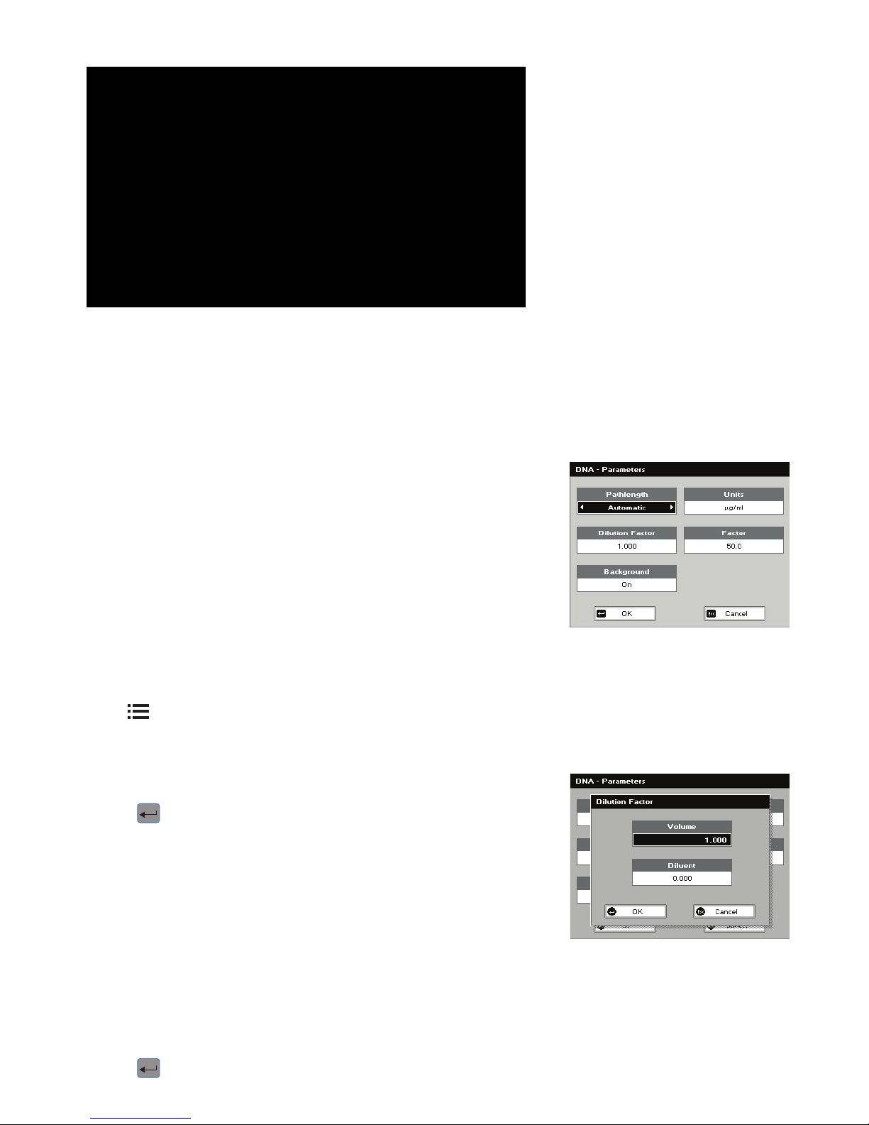
4.2.2. DNA measurement

The procedure is as follows:

Step 1

Press 1 to select DNA mode.

Step 2

Select Pathlength using the left and right arrows. Options are 0.5 mm, 0.2 mm or Automatic. Press the down arrow.

Step 3 (Dilution Factor known) Enter the Dilution Factor using the keypad numbers (range 1.00 to 9999). Use the C button to backspace and clear the last digit entered.

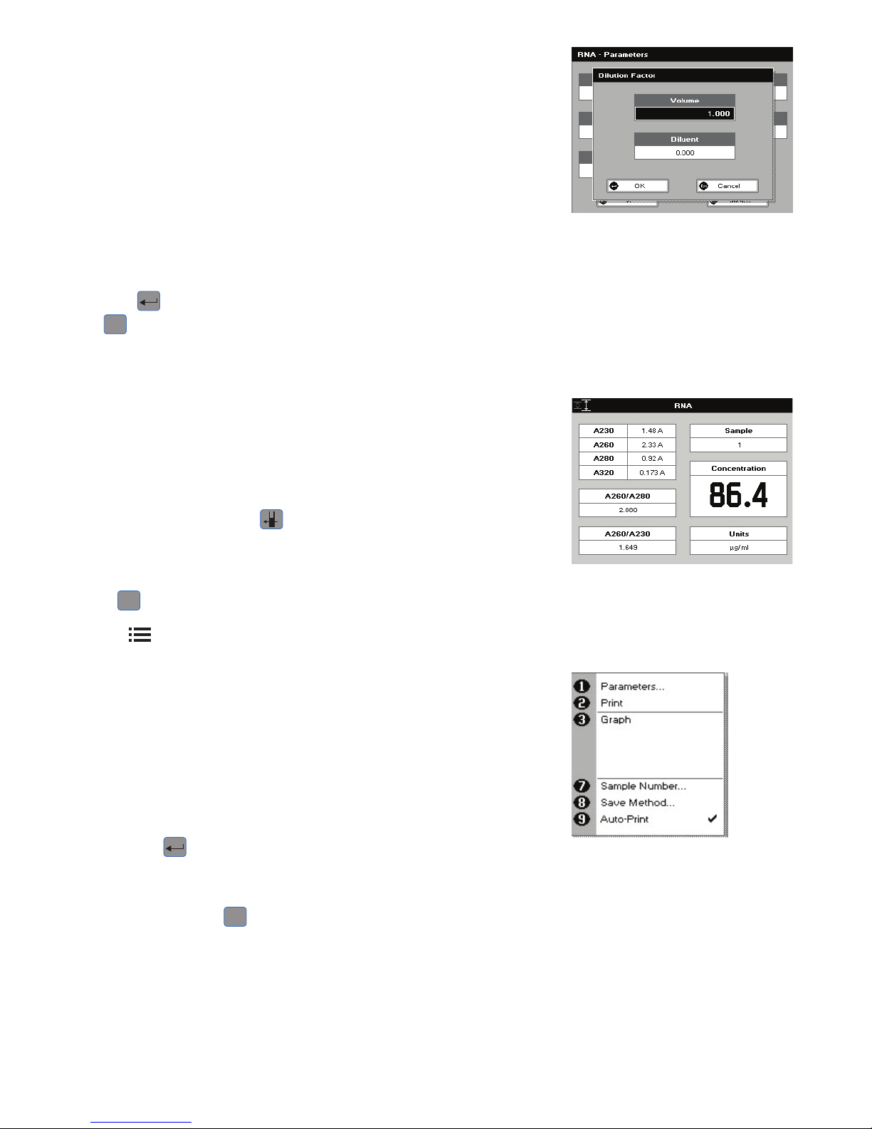
Step 3 (calculate Dilution Factor) Press

 to enter the Dilution Factor Screen (see second parameter screen to

the left).

Enter the Volume of the sample using the keypad numbers (range 0.01 to 9999). Press the down arrow.

Enter the volume of the Diluent using the keypad numbers (range 0.01 to 9999).

Press OK

to calculate the Dilution Factor and return to the Parameters Screen

OR Press Cancel to cancel the selections and return to the Parameters Screen.

Step 4

Background Correction at 320 nm will be on. It may be turned off with the left or right arrows. Press the down arrow.

Step 5

Select the Units of measurement using the left and right arrows. Options: µg/ml, ng/µl, µg/µl. Press the down arrow.

Step 6

Enter the Factor using the keypad numbers. The default value is 50, the range is

0.01 to 9999.

Step 7 Press OK

to enter the Results Screen and begin making measurements.

Typical spectral scan of a Nucleic Acid:-

Page 17

5061-049 REV 1.4

Esc

to return to the Life Science Screen.

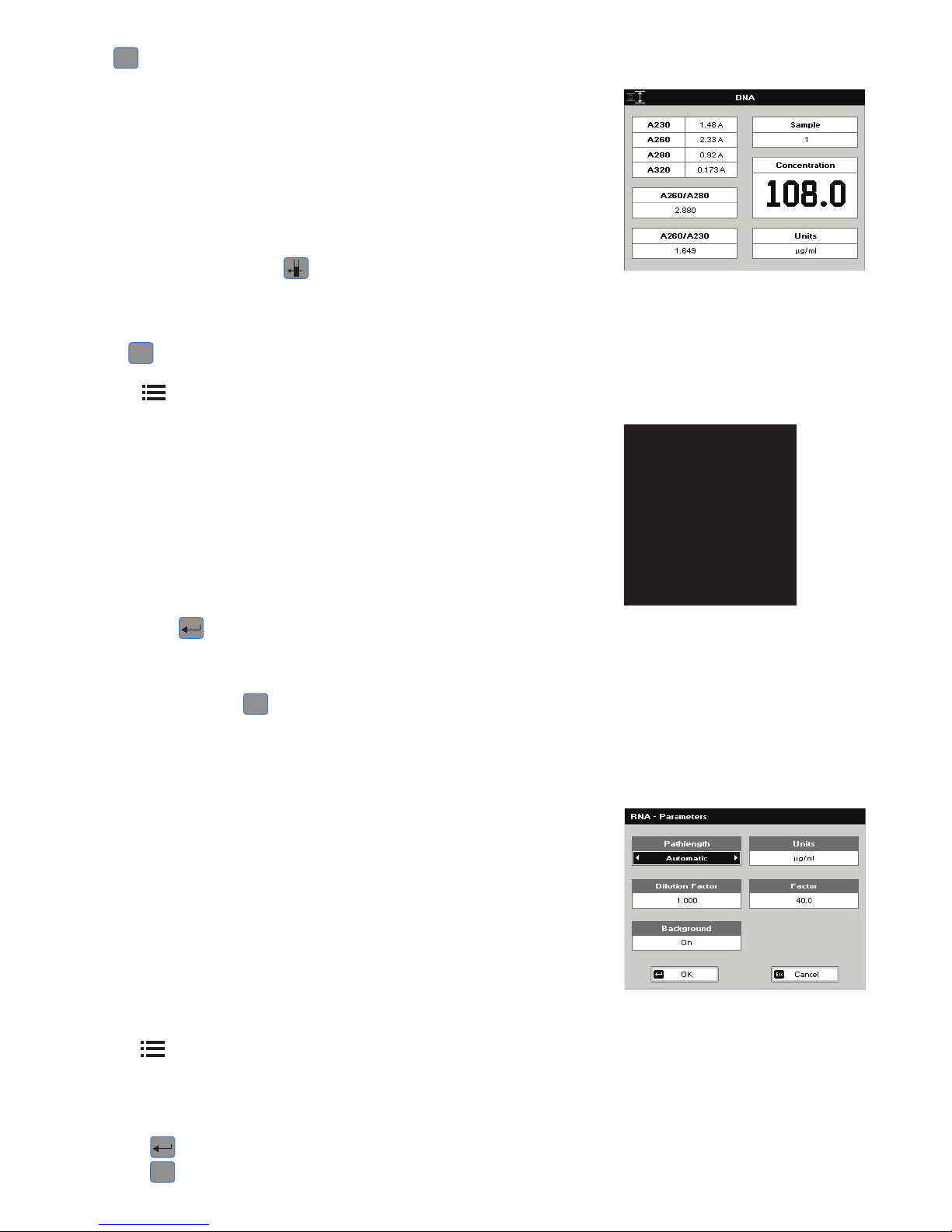
Results Screen

Step 8

Pipette on the reference sample and lower the sampling head. If Auto-Read is off, press the 0A/100%T key. This will be used for all subsequent samples until changed. If QA is switched on the sample will need to be replaced and the 0A/100% T key pressed again.

Step 9

Clean the top and bottom plates, pipette on the sample and lower the sampling head. If Auto-Read is off, press

. This measures at the selected wavelengths and displays the results. The ratio of the Absorbance values at wavelengths 1 and 2 are calculated. The Concentration is based on the Absorbance at wavelength 1. Repeat step 9 for all samples.

Press

Esc

to return to the Life Science Screen.

Press

 to display available Options which are described below.

Options (select using keypad numbers)

1. Return to Parameters Screen (step 1 above).

2. Print result via selected method.

3. Toggle Graph on/off. The graph shows a Wavescan plot across the range

220 nm to 320 nm with cursors denoting 230, 260, 280 and (if Background Correction selected) 320 nm.

7. Sample Number – add a prefix to the sample number and reset the

incrementing number to the desired value.

8. Save Method – use the alpha-numeric keys to enter a name for the method and

press Save

9. Auto-Print – toggles Auto-Print on/off.

Exit Options by pressing

Esc

or wait.

4.2.3. RNA measurement

The procedure is as follows:

Step 1

Press 2 to select RNA mode.

Step 2

Select Pathlength using the left and right arrows. Options are 0.5 mm, 0.2 mm or Automatic. Press the down arrow.

Step 3 (Dilution Factor known)

Enter the Dilution Factor using the keypad numbers (range 1.00 to 9999). Use the C button to backspace and clear the last digit entered.

Step 3 (calculate Dilution Factor)

Press

 to enter the Dilution Factor Screen (see second image to the left).

Enter the Volume of the sample using the keypad numbers (range 0.01 to 9999).

Press the down arrow.

Enter the volume of the Diluent using the keypad numbers (range 0.01 to 9999).

Press OK

to calculate the Dilution Factor and return to the Parameters Screen.

OR Press

Esc

to cancel the selections and return to the Parameters Screen.

Page 18

5061-049 REV 1.4

Step 4

Select whether the Background Correction at 320 nm is to be used or not with the left and right arrows.

Press the down arrow.

Step 5

Select the Units of measurement using the left and right arrows. Options: µg/ml, ng/µl, µg/µl.

Press the down arrow.

Step 6

Enter the Factor using the keypad numbers. The default value is 40, the range is

0.01 to 9999.

Step 7

Press OK

to enter the Results Screen and start making measurements.

Esc

to return to the Life Science Screen.

Results Screen

Step 8

Step 9

Clean the top and bottom plates, pipette on the sample and lower the sampling head. If Auto-Read is off, press

. This measures at the selected wavelengths

and displays the results. The ratio of the Absorbance values at wavelengths 1 and 2 are calculated. The Concentration is based on the Absorbance at wavelength 1.

Repeat step 9 for all samples.

Press

Esc

to return to the Life Science Screen.

Press

 to display available Options which are described below.

Options (select using keypad numbers)

1. Return to Parameters Screen (step 1 above).

2. Print result via selected method.

3. Toggle Graph on/off. The graph shows a Wavescan plot across the range

220 nm to 320 nm with cursors denoting 230, 260, 280 and (if Background Correction selected) 320 nm.

7. Sample Number – add a prefix to the sample number and reset the incrementing number to the desired value.

8. Save Method – use the alpha-numeric keys to enter a name for the method and press Save

9. Auto-Print – toggles Auto-Print on/off.

Exit Options by pressing

Esc

, or wait.

Page 19

5061-049 REV 1.4

4.2.4. Oligonucleotide measurement

The procedure is as follows:

Step 1

Press 3 to select Oligo mode.

Step 2

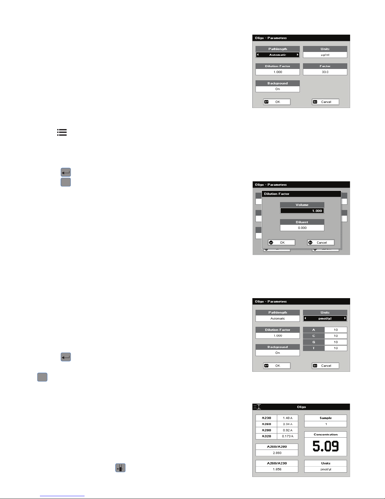
Select Pathlength using the left and right arrows. Options are 0.5 mm, 0.2 mm or Automatic. Press the down arrow.

Step 3 (Dilution Factor known) Enter the Dilution Factor using the keypad numbers (range 1.00 to 9999). Use the C button to backspace and clear the last digit entered.

Step 3 (calculate Dilution Factor) Press

 to enter the Dilution Factor Screen.

Enter the Volume of the sample using the keypad numbers (range 0.01 to 9999).

Press the down arrow.

Enter the volume of the Diluent using the keypad numbers (range 0.01 to 9999).

Press OK

to calculate the Dilution Factor and return to the Parameters Screen.

OR Press

Esc

to cancel the selections and return to the Parameters Screen.

Step 4

Select whether the Background Correction is to be used or not with the left and right arrows.

Press the down arrow.

Step 5

Select the Units of measurement using the left and right arrows. Options: µg/ml, ng/µl, µg/µl and pmol/µl. If pmol/µl is selected the factor changes to a selection table denoting the ratios of the 4 bases in the structure.

Press the down arrow.

Step 6 (Units not pmol/µl) Enter the factor using the keypad numbers. The default value is 33, the range is

0.01 to 9999.

Step 6 (Units pmol/µl) Enter the proportions of bases present using the keypad numbers and up and down arrows to move between boxes. The default is 10 for each, the range is 0 to

9999.

Step 7

Press OK

to enter the Results Screen and start making measurements

Esc

to return to the Life Science Screen.

Results Screen

Step 8

Step 9

Clean the top and bottom plates, pipette on the sample and lower the sampling head. If Auto-Read is off, press

. This measures at the selected wavelengths

Page 20

5061-049 REV 1.4

and displays the results. The ratio of the Absorbance values at wavelengths 1 and 2 are calculated. The Concentration is based on the Absorbance at wavelength 1.

Repeat step 9 for all samples.

Press

Esc

to return to the Life Science Screen.

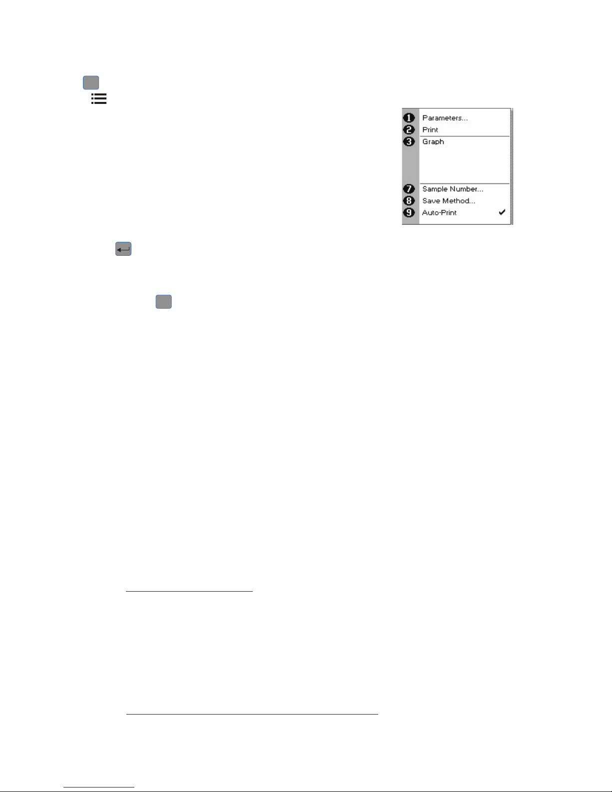
Press



to display available Options which are described below.

Options (select using keypad numbers)

1. Return to Parameters Screen (step 1 above).

2. Print result via selected method.

3. Toggle Graph on/off. The graph shows a Wavescan plot across the range

220 nm to 320 nm with cursors denoting 230, 260, 280 and (if Background Correction is selected) 320 nm.

7. Sample Number – add a prefix to the sample number and reset the incrementing number to the desired value.

8. Save Method – use the alpha-numeric keys to enter a name for the method and press Save

9. Auto-Print – toggles Auto-Print on/off.

Exit options by pressing

Esc

, or wait.

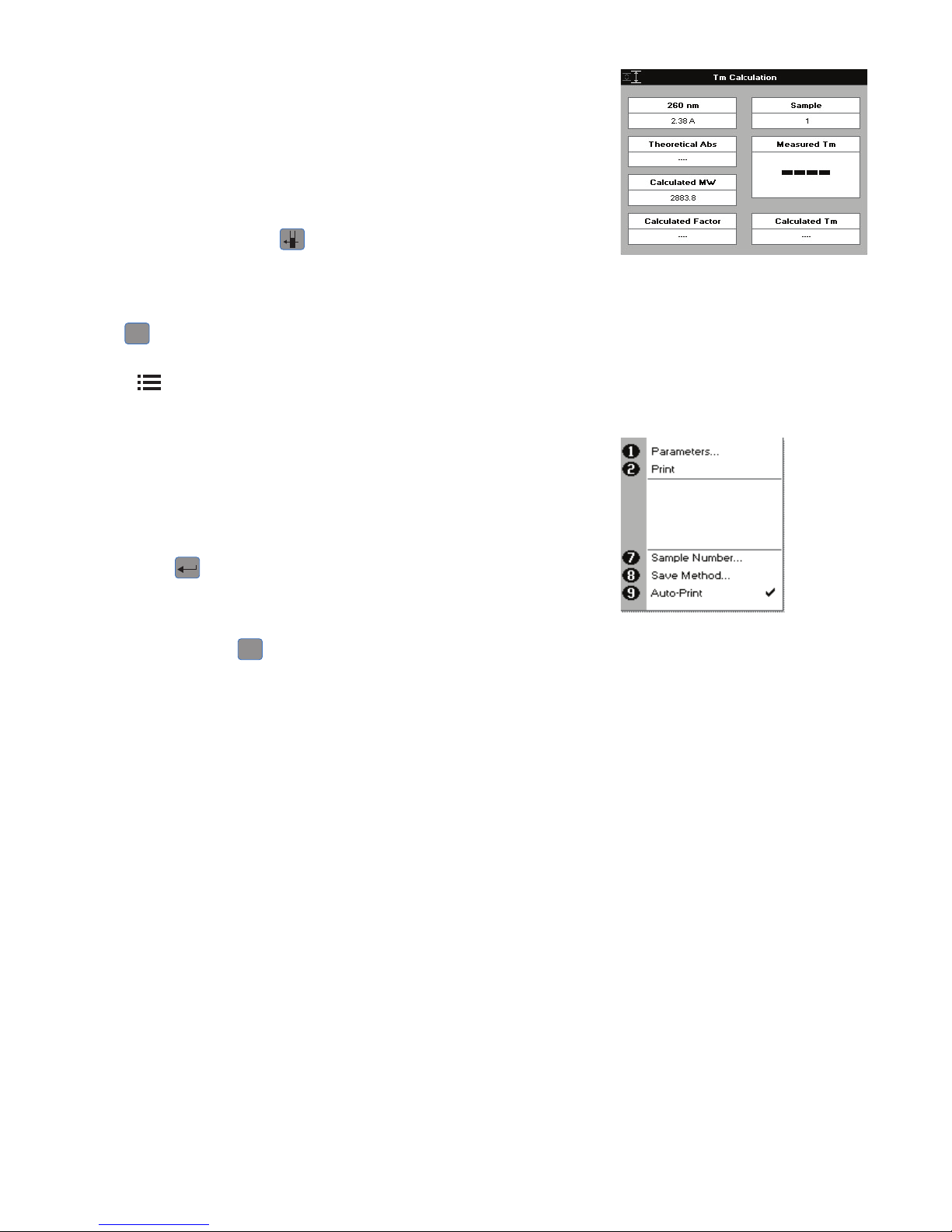
4.2.5. Tm Calculation

This utility calculates the theoretical melting point from the base sequence of a primer. It is done using nearest neighbor thermodynamic data for each base in the nucleotide chain in relation to its neighbor (Breslauer et al, Proc.Natl. Acad. Sci. USA Vol 83, p3746 1986). The data obtained are useful both in the characterization of oligonucleotides and in calculating Tm for primers used in PCR experiments.

The ACGT/U sequence entered into the utility is used to calculate the theoretical T

, the theoretical Absorbance (Absorption units/mmol) and the conversion factor (mg/ml). This is because the stability of a bent and twisted sequence of bases such as an oligonucleotide is dependent on the actual base sequence. The calculated

thermodynamicinteractionsbetweenadjacentbasepairshavebeenshownto

correlate well with experimental observations. This utility uses matrices of known, published thermodynamic values and extinction

coefficients to calculate T

and the theoretical Absorbance/factor respectively of an

entered base sequence.

This is calculated using the equation:-

Tm = ∆H × 100

- 273.15 +16.6 log [salt]

∆S + (1.987 × loge(c/4 +53.0822)

where ∆H and ∆S are the enthalpy and entropy values summed from

respective 2 × 4 × 4 nearest neighbor matrices

c is the Primer concentration of oligonucleotide (pmoles/ml) in the

calculated Tm or the measured concentration in measured Tm. In the latter case concentration is obtained from the equation:

c = Abs(260 nm) × Calculated factor × pathlength multiplier × 10 000 MW

Page 21

5061-049 REV 1.4

Calculated factor and MW are defined below

[salt] is the buffer molarity plus total molarity of salts in the hybridization

solution (moles/l)

Weights for ∆Sareindexedbyadjacentpairedbases.

A similar equation applies to weights for ∆H,againindexedbyadjacentbases.

Note that bivalent salts may need normalizing using a multiplying factor of 100 because of their greater binding power.

Theoretical Absorbance

The Theoretical Absorbance is based on a calculation as follows:

Foreachadjacentpairofbases(nearestneighbors)anextinctioncoefficientweight

is accumulated using a 4 × 4 table (one for either DNA or RNA). This total weight is doubled and then for each internal base a counterweight is subtracted using another 1 × 4 table. The end bases are excluded from the latter summation.

That is:

Total Extinction Coefficient E = ∑ (2 × aTable[base_type][base(n)][base(n+1)])

- ∑ (tTable[base_type][base(n]])

Conversion factor

The Conversion Factor is given by = Molecular weight

ABCDE

∑ E

ABCDE

where E

ABCDE

= [ 2 × (EAB +EBC +ECD +EDE) –EB –EC –ED ]

•Themolecularweight(MW)ofaDNAoligonucleotideiscalculatedfrom:

MW (g/mole) = [(dA × 312.2) + (dC × 288.2) + (dG × 328.2) + (dT × 303.2.)] + [(MW counter-ion) × (length of oligo in bases)]

(for RNA oligonucleotide, (dT × 303.2) is replaced by (dU × 298.2)

 TheMWcalculatedusingthisequationmustbeadjustedforthecontributionof

the atoms at the 5’ and 3’ ends of the oligo.

For phosphorylated oligos: add: [17 + (2 × MW of the counter-ion)] For non-phosphorylated oligos: subtract: [61 + (MW of the counter-ion)]

The MW (g/mole) of the most common oligo counter-ions are; Na (sodium) 23.0 K (potassium) 39.1 TEA (triethylammonium) 102.2 Other Defaults to 1.0 (H) Variable 0.1–999.9 in next option box.

Calculated molecular weight: a weight is added for each base looked up from a table. The weight of the counter ion is added for every base from a small table for the known ions. If phosphorylated, then the system adds 17.0 plus two counter ions otherwise it subtracts 61.0 and one ion.

TheoreticalAbsorbance:foreachadjacentpairofbases(nearestneighbors)a

weight is accumulated using a table. For each internal base a weight is subtracted using another table. Separate tables are used for DNA and RNA.

Page 22

5061-049 REV 1.4

Calculated factor:thisisjustthecalculatedmolecularweightdividedbythe

theoretical Absorbance.

The procedure is as follows:

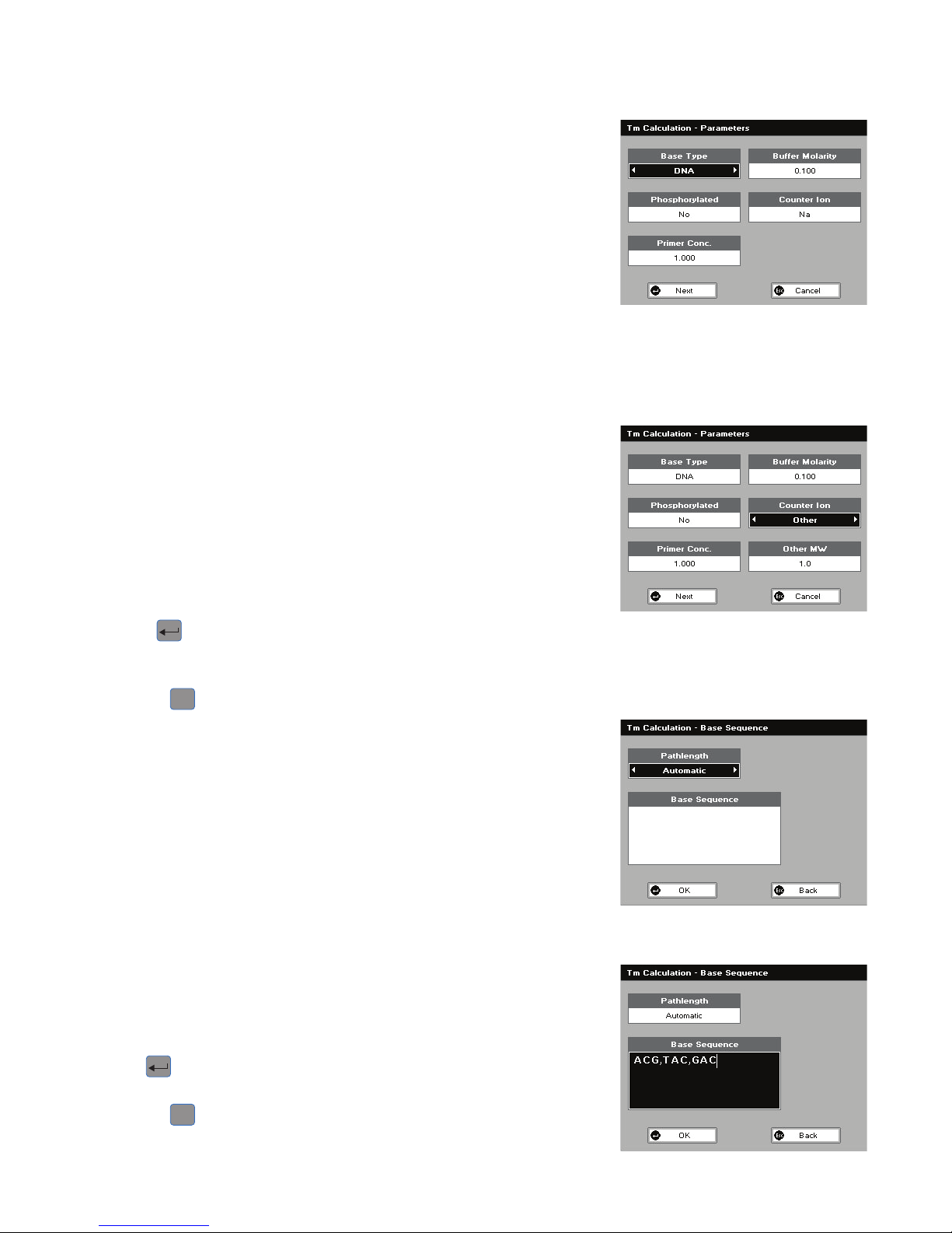
Step 1

Press 4 to enter the Tm Calculation Parameters Screen.

Step 2 Select the Base Type: DNA or RNA.

Press the down arrow.

Step 3 Select whether the sample is Phosphorylated or not (Yes or No).

Press the down arrow.

Step 4 Enter the Primer Conc. using the keypad numbers (range 0.000 to 99.9) in pmole/ml.

Press the down arrow.

Step 5 Enter the Buffer Molarity (buffer molarity + total molarity of salt in moles/l) using the keypad numbers (range 0.000 to 10).

Press the down arrow.

Step 6 Select the Counter Ion: Na, K, TEA or Other.

Step 7 (if Other selected, see the previous section)

Enter the molecular weight (Other MW) of the Counter Ion used.

Step 8 Press Next

to select these parameters and go on to the Base Sequence

Screen

Press Cancel

Esc

to return to the Life Science Screen.

Step 9 Select the Pathlength of the sample cells. Options are 0.5 mm, 0.2 mm or Automatic.

Step 10 Enter the known Base Sequence triplets using the number keys: 1 for A, 3 for C, 4 for G and 6 for T or U. Note that a comma is added after each triplet to improve readability

Step 11 Press OK

to select these parameters and start to measure Tm

Press Cancel

Esc

to return to the Parameters Screen.

Page 23

5061-049 REV 1.4

Results Screen

Step 12

Step 13 Clean the top and bottom plates, pipette on the sample and lower the sampling head. If Auto-Read is off, press

. The unit measures the Absorbance and uses

this information to calculate the Measured Tm.

Repeat step 13 for all samples.

Press

Esc

to return to the Life Science Screen.

Press



to display available Options which are described below.

Options (select using keypad numbers)

1. Return to Parameters Screen (step 1 above).

2. Print result via selected method.

7. Sample Number – add a prefix to the sample number and reset the

incrementing number to the desired value.

8. Save Method – use the alpha-numeric keys to enter a name for the method and press Save

9. Auto-Print – toggles Auto-Print on/off.

Exit options by pressing

Esc

, or wait.

4.2.6. CyDye measurement

Measurement of the labeling efficiency of fluorescently labeled DNA probes before 2-color microarray hybridization ensures that there is sufficient amount of each probe to give satisfactory hybridization signals. These data also provide an

opportunitytobalancetherelativeintensitiesofeachfluorescentdyebyadjusting

the concentration of each probe before hybridization. The DNA yield is measured at 260nm while the incorporation of fluorescein, Cy3, Cy5 and other dyes are measured at their absorption peaks. This method may also be useful for measuring the yields and brightness of fluorescently labeled in-situ hybridization probes.

Equations used in the software are detailed below:

DNA Concentration = (A

260

– A

Background

) * NucleicAcid Factor

DNA Quantity = DNAConcentration * Volume

Dye Concentration = ((A

Dye

- A

Background

) / ExtinctionCoefficient

Dye

) * PathlengthFactor * Dilution_Factor

* 10

Dye Quantity = DyeConcentration * Volume

Page 24

5061-049 REV 1.4

Dye Incorporation = DyeQuantity / DNAQuantity

Dye FOI = DyeQuantity * (324.5 / DNAQuantity)

Step 1 Press 5 to enter the Cy Dye Parameter Screen from the Life Sciences screen.

Step 2 Either select the Dye Name of the dye being used by using the left and right arrows, or select “Custom” if you wish to create a new entry. If a standard dye is selected, press Next to move to the next screen (Step 7). If “Custom” has been selected press the down arrow.

Step 3 (Custom only) Enter the Wavelength of the dye peak Absorbance.

Press the down arrow.

Step 4 (Custom only) Enter the dye Extinction Coefficient.

Press the down arrow.

Step 5 (Custom only) Enter the dye 260 nm Correction factor (if known), otherwise set at zero.

Step 6 (Custom only) Enter a name for the dye to identify it correctly.

To complete the entry press Next

to enter the second dye detail entry screen.

Press Cancel

Esc

to return to the Life Science Screen.

Step 7 If there is no second dye select None, otherwise proceed as for Dye 1.

Press Next

to complete data entry and enter the Parameter screen

Press Cancel

Esc

to return to the Dye 1 data entry screen.

Step 8

If the concentration is known select the appropriate Pathlength, otherwise leave it as Automatic

Step 9 Unless there are complicating absorbencies at the Background wavelength, leave this as On.

Step 10 If using standard dyes, the Background Wavelength is set automatically, but if there are interferences at this default wavelength, the user can select a wavelength where the background is at or close to the reference sample. If no such wavelength is available set the previous box Background Correction to Off. This will give rise to noisier results though

Page 25

5061-049 REV 1.4

Step 11 Enter the Dilution Factor (if applicable)

Step 12 (Dilution Factor known)

Enter the Dilution Factor using the keypad numbers (range 1.00 to 9999). Use the C button to backspace and clear the last digit entered.

Step 13 (calculate Dilution Factor)

Press

 to enter the Dilution Factor Screen (see right). Enter the Volume of

the sample using the keypad numbers (range 0.01 to 9999). Press the down arrow.

Enter the volume of the Diluent using the keypad numbers (range 0.01 to 9999).

Press OK

to calculate the Dilution Factor and return to the Parameters Screen.

OR Press

Esc

to cancel the selections and return to the Parameters

Step 14

Select the Nucleic acid being used (or none if only the dye is being measured). The system will select the appropriate factor. If a different factor is desired select Custom and the Factor can be user defined.

Press OK

to enter the Results screen.

OR Press

Esc

to cancel the selections and return to the Parameters data entry

screen.

Step 15

Pipette on the reference sample and lower the sampling head. If Auto-Read is off, press the 0A/100%T key. This will be used for all subsequent samples until changed. If QA is switched on the reference sample will need to be replaced and the 0A/100% T key pressed again.

Step 16

Clean the top and bottom plates, pipette on the sample and lower the sampling head. If Auto-Read is off, press

. The system returns the dye concentration(s).

Repeat step 17 for all samples.

Press

Esc

to return to the Life Science Screen.

Press



to display available Options which are described below.

Note that very high dye concentrations may leave visible deposits on the sample plates. This can easily be removed with a gentle rub with ethanol.

Options (select using keypad numbers)

Page 26

5061-049 REV 1.4

1. Return to Parameters Screen (step 1 above).

2. Print result via selected method.

3. Toggle Graph on/off. The graph shows the spectral scan of the dye sample over

the wavelength range of interest.

4. Toggle Results on/off. When off, the results screen shows the details for the dye concentration, Frequency of Incorporation (FOI) and incorporation. When on, (see picture to left) the results screen shows the DNA Concentration and DNA quantity. This only functions if the graph display is off.

5. Sample Number – add a prefix to the sample number and reset the incrementing number to the desired value.

6. Save Method – use the alpha-numeric keys to enter a name for the method and press Save

7. Auto-Print – toggles Auto-Print on/off.Exit options by pressing

Esc

, or wait.

4.3. Proteins

4.3.1. Theory

Protein Determination at 280 nm

Protein can be determined in the near UV at 280 nm due to absorption by tyrosine, tryptophan and phenylalanine amino acids. The Abs280 varies greatly for different proteins due to their amino acid content and consequently the specific Absorption value for a particular protein must be determined.

•Thepresenceofnucleicacidintheproteinsolutioncanhaveasignificanteffect

due to strong nucleotide Absorbance at 280 nm. This can be compensated by measuring Abs260 and applying the equation of Christian and Warburg for the protein crystalline yeast enolase (Biochemische Zeitung 310, 384 (1941)):

Protein (mg/ml) = 1.55 * Abs280 - 0.76 * Abs260 (where * means “multiplied by”)

or,

Protein conc. = (Factor 1 * Abs280) - (Factor 2 * Abs260)

•Thisequationcanbeappliedtootherproteinsifthecorrespondingfactorsare

known. NanoVue Plus can determine protein concentration at 280 nm and uses the above equation as default. The factors can be changed and the use of Background Correction at 320 nm is optional.

•Tocustomisetheequationforaparticularprotein,theAbsorbancevaluesat260

and 280 nm should be determined at known protein concentrations to generate simple simultaneous equations; solving these provides the two coefficients. In cases where Factor 2 is found to be negative, it should be set to zero since it means there is no contribution to the protein concentration due to Absorbance at 260 nm.

•SetFactor2=0.00fordirectλ280 UV protein measurement. Factor 1 is based on the extinction coefficient of the protein.

•IntheProteinA280application,variousmodescanbeselecteddependingon

the extinction coefficient of the reference protein being used.

A) If the mode is Christian Warburg, the equation given above is used.

B) For BSA the extinction coefficient is 6.7 AU (E1%) at Abs 280 for a 1% ww

solution

Page 27

5061-049 REV 1.4

C) For IgG the extinction coefficient is 13.7 AU (E1%) at Abs 280 for a 1% ww

solution

D) For lysozyme the extinction coefficient is 26.4 AU (E1%) at Abs 280 for a 1% ww

solution.

E) For other reference proteins the user can enter; the molar extinction coefficient

and the molecular weight of the protein, the mass extinction coefficient for a 1% solution, or the E1% value.

The expressions are:

Molar Extinction: Conc in ug/ml = (A280* kDa * 1000) / em

where em = molar extinction coefficient (em) M

-1cm-1

kDa = molecular weight in kiloDaltons.

Mass extinction: Conc in ug/ml .= (A280 *1000) / ema

where ema = mass extinction coefficient ema (equivalent to Absorbance of 1 g/l solution).

E1%: Conc in ug/ml = (A280 *10000) / E1%

where E1% = extinction coefficient E1% (g/100 ml)

-1

(equivalent to the inverse of the 10 mm Absorbance of a 1% solution of the protein under test).

•RapidmeasurementssuchasthisatAbs280areparticularlyusefulafterthe

isolation of proteins and peptides from mixtures using spin and HiTrap columns by centrifuge and gravity, respectively.

Protein Determination at 595, 546, 562 and 750 nm

•TheBradfordmethoddependsonquantifyingthebindingofadye,Coomassie

Brilliant Blue, to an unknown protein and comparing this binding to that of different, known concentrations of a standard protein at 595 nm; this is usually BSA (bovine serum albumin).

•TheBiuretmethoddependsonreactionbetweencupricionsandaminoacid

residues in an alkali solution, resulting in the formation of a complex absorbing at 546 nm.

•TheBCAmethodalsodependsonreactionbetweencupricionsandamino

acid residues, but in addition combines this reaction with the enhancement of cuprous ion detection using bicinchoninic acid (BCA) as a ligand, giving an Absorbance maximum at 562 nm. The BCA process is less sensitive to the presence of detergents used to break down cell walls.

•TheLowrymethoddependsonquantifyingthecolorobtainedfromthereaction

of Folin-Ciocalteu phenol reagent with the Tyrosyl residues of an unknown protein and comparing with those derived from a standard curve of a standard protein at 750 nm; this is usually BSA.

•Detailedprotocolsaresuppliedwiththeseassaykits,andmustbeclosely

followed to ensure accurate results are obtained. The small sample size required with NanoVue Plus may allow modification of the manufacturer’s protocols and considerable economies may be made at the user’s discretion.

•Touseazeroconcentrationstandard,includeitinthenumberofstandardsto

be entered and enter 0.00 for concentration; use this when required to enter standard 1.

•Alinearregressionanalysisofthecalibrationstandarddatapointsiscalculated;

the result, together with the correlation coefficient, can be printed out. A correlation coefficient of between 0.95 and 1.00 indicates a good straight line.

Page 28

5061-049 REV 1.4

Use of Background Correction

•BackgroundCorrectionatawavelengthwellapartfromtheproteinpeakisused

to compensate for the effects of background Absorbance. The procedure can

adjustfortheeffectsofturbidity,strayparticulatesandhigh-Absorbancebuffer

solutions.

•NanoVuePlususesBackgroundCorrectionat320nm.Itisparticularly

recommended since very small samples are particularly susceptible to stray particulates. The Background function toggles On and Off with either left/right arrows from the relevant page.

•I f itisused,therewillbedifferentresultsfromthosewhenunused,because Abs 320 is subtracted from the Abs 280 value prior to use in the above equations.

•Backgroundcorrectionisnotusedinmethodsthatusetestkitssuchasthe

Bradford, Biruet, BCA and Lowry applications

4.3.2. Protein UV

This is the Christian and Warburg assay discussed above. The procedure is as follows:

Step 1 Press 1 to select Protein UV mode.

Step 2 Select Pathlength using the left and right arrows. Options are 0.5 mm, 0.2 mm or Automatic.

Press the down arrow.

Step 3 (Dilution Factor known) Enter the Dilution Factor using the keypad numbers (range 1.00 to 9999). Use the C button to backspace and clear the last digit entered.

Step 3 (calculate Dilution Factor) Press

 to enter the Dilution Factor Screen, shown to the left.

Enter the Volume of the sample using the keypad numbers (range 0.01 to 9999).

Press the down arrow.

Enter the volume of the Diluent using the keypad numbers (range 0.01 to 9999).

Press OK

to calculate the Dilution Factor and return to the Parameters Screen.

OR Press

Esc

to cancel the selections and return to the Parameters Screen.

Step 4 Select whether the Background Correction is to be used or not with the left and right arrows.

Press the down arrow.

Step 5 Enter the Abs260 Factor using the keypad numbers (see method described in introduction). The default value is 0.76, the range is 0.000 to 9999.

Press the down arrow.

Step 6 Enter the Abs280 Factor using the keypad numbers (see method described in introduction). The default value is 1.55, the range is 1.000 to 9999.

Press the down arrow.

Step 7 Select the Units of measurement using the left and right arrows. Options: µg/ml, ng/µl and µg/µl.

Page 29

5061-049 REV 1.4

Step 8 Press OK

to enter the Results Screen

Cancel

Esc

to return to the Protein Screen.

Results Screen

Step 9

Step 10 Clean the top and bottom plates, pipette on the sample and lower the sampling head. If Auto-Read is off, press

. This measures at both 260 and 280 nm

wavelengths and displays the Protein concentration as the Result.

Repeat step 10 for all samples.

Press

Esc

to return to the Protein Screen.

Press

 to display available Options which are described below.

Options (select using keypad numbers)

1. Return to Parameters Screen (step 1 above).

2. Print result via selected method.

3. Toggle Graph on/off. The graph shows a wavescan plot across the range

220 nm to 330 nm with cursors denoting 230, 260, 280 and (if background correction selected) 320 nm.

7. Sample Number – add a prefix to the sample number and reset the incrementing number to the desired value.

8. Save Method – use the alpha-numeric keys to enter a name for the method and press Save

9. Auto-Print – toggles Auto-Print on/off.

Exit Options by pressing

Esc

, or wait.

Page 30

5061-049 REV 1.4

4.3.3. Protein A280

Step 1

Press 2 to select Protein A280.

Step 2 Select the Mode. Options are Christian Warburg, BSA, IgG, Lysozyme, Molar extinction, Mass extinction, E 1%.

Step 3 Select Pathlength using the left and right arrows. Options are 0.5 mm, 0.2 mm or Automatic.

Press the down arrow. Step 4 (Dilution Factor known) Enter the Dilution Factor using the keypad numbers (range 1.000 to 9999). Use the

C button to backspace and clear the last digit entered. OR

Step 4 (calculate Dilution Factor) Press



to enter the Dilution Factor Screen, shown to the left. Enter the Volume of the sample using the keypad numbers (range 0.001 to 9999). Press the down arrow. Enter the volume of the Diluent using the keypad numbers (range 0.001 to 9999). Press OK

to calculate the Dilution Factor and return to the Parameters Screen. OR Press

Esc

to cancel the selections and return to the Parameters Screen.

Step 5 Select whether Background Correction is to be used or not with the left and right arrows.

Press the down arrow.

Step 6 (Mode = Christian Warburg, BSA, IgG, Lysozyme) Select the Units of measurement using the left and right arrows. Options: mg/ml, µg/ml, ng/µl and µg/µl.

Step 6 (Mode = Molar extinction) Enter the Value for the molar extinction coefficient of the protein reference being used (units l/mol). The default value is 50.

Press the down arrow.

Step 7 (Mode = Molar extinction) Enter the Molecular Weight of the reference protein in kilo Daltons. The default value is 50.

Step 6 (Mode = Mass extinction) Enter the Mass Extinction Coefficient for the protein reference being used (units l/g). The default value is 50.

Step 6 (Mode = E 1%) Enter the Mass Extinction Coefficient for a 10 mg/ml(1%) solution of the reference protein. The default value is 50.

Step 8 (all modes) Press OK

to enter the Results Screen OR Cancel

Esc

to return to the Protein Screen.

Results Screen

Step 9

Page 31

5061-049 REV 1.4

Step 10 Clean the top and bottom plates, pipette on the sample and lower the sampling head. If Auto-Read is off, press . This measures at both 260 and 280 nm wavelengths and displays the Protein concentration as the Result.

Repeat step 10 for all samples.

Press

Esc

to return to the Protein Screen.

Press

 to display available Options which are described below.

Options (select using keypad numbers)

1. Return to Parameters Screen (step 1 above).

2. Print result via selected method.

3. Toggle Graph on/off. The graph shows a wavescan plot across the range 250 nm

to 330 nm.

7. Sample Number – add a prefix to the sample number and reset the incrementing number to the desired value.

8. Save Method – use the alpha-numeric keys to enter a name for the method and press Save

9. Auto-Print – toggles Auto-Print on/off.

Exit Options by pressing

Esc

, or wait.

4.3.4. BCA

The procedure is as follows:

Step 1 Press 3 to select BCA mode.

Step 2 The Wavelength for this method is fixed at 562 nm.

Step 3 Enter the number of Standards (1–9) to be used in the curve using the keypad numbers or left and right arrows.

Press the down arrow.

Step 4 (see second image) Units: The user can enter a text string up to 8 characters long. To access a list of pre-defined units press the Options key

 and then use the left/right arrows

to select from µg/ml, µg/µl, pmol/µl, mg/dl, mmol/l, µmol/l, g/l, mg/l, µg/l, U/l, %, ppm, ppb, conc or none. These units can also be edited once OK is pressed.

This screen also allows the number of displayed decimal points (DP) to be selected, from 0 to 2. Note that the result will always be fixed to 5 significant figures regardless of how many decimal points are selected (so 98768.2 will display as 98768 even with 1 decimal point selected).

Press OK

to store the chosen parameters or Cancel

Esc

Step 5 Enter the Pathlength. Options are 0.5 mm or 0.2 mm.

Press Next

to move on to the next parameters screen or

Esc

Cancel to return

to the Protein Screen.

Step 6 Enter the type of Curve Fit. Options are Regression (straight line), Zero Regression (forces the straight line through the origin), Interpolated or Cubic Spline.

Press the down arrow.

, 2nd order polynomial.

Page 32

5061-049 REV 1.4

Step 7 Select the Calibration Mode, either Standards (measure prepared standards), Manual (keypad data entry, go to step 9), or New Standards (means new standards are measured each time the method is used).

Step 8 (only if Standards is selected) Select the number of Replicates using the left and right arrows. This determines the number of standards to be measured and averaged at each standard concentration point. Can be Off, 2 or 3.

Press Next

to enter the Standards Screen

Press Cancel

Esc

to cancel selections and return to the Protein Screen.

Standards Screen

Step 9 (Standards/Manual selected)

Enter the concentration values by using the keypad numbers and the up and down arrows to move between the different standard boxes (range 0.001 to 9999). C button backspaces and clears the last digit entered.

Step 10 (Standards/Manual selected)

Press Next

to enter the Calibration Screen. If there are duplicate or non-

monotonic (increasing) entries, the unit will beep and highlight the incorrect entry.

OR Press Back

Esc

to return to the Parameters Screen.

Calibration Screen (Replicates off) This shows the calibration values and allows standards to be measured or entered using the keypad numbers (if calibration mode is Manual).

Step 11 (Standards selected) Pipette on the reference sample and lower the sampling head. If Auto-Read is off, press the 0A/100%T key. This will be used for all subsequent samples until changed. If QA is switched on the sample will need to be replaced and the 0A/100% T key pressed again.

Step 12 (standards selected) Clean the top and bottom plates, pipette on the standard and lower the sampling head. If Auto-Read is off, press

, (use C to clear previously stored results before

measuring) to measure the standard and store the result.

Repeat step 12 for all standards. A graph will display the results and the fitted curve as the measurements are made.

Use the up and down arrows to select a standard to be repeated if a poor reading has been obtained. Use C to clear the previous reading.

Step 13 (Standards/Manual selected) When all standards are measured the OK box appears. Press OK

to accept the

calibration and go to the Results Screen (see below)

Press Back

Esc

to cancel selections and return to the Standards Screen.

Calibration Screen (Replicates on)

This shows the calibration values and allows standards to be measured.

Step 11 (Standards selected)

Pipette on the reference sample and lower the sampling head. If Auto-Read is off, press the 0A/100%T key. This will be used for all subsequent samples until changed.

Page 33

5061-049 REV 1.4

Step 12 (Standards selected)

Press Replicates

to display the replicate entry boxes. Use C to clear previously

stored results before measuring.

Clean the top and bottom plates, pipette on the replicate standard and lower the sampling head. If Auto-Read is off, press

to measure the standard and store

the result.

Repeat for all replicates and standards. Use Next

to bring up fields for the next standard. A graph will display the results and the fitted curve as the measurements are input.

Use the up and down arrows to select a standard to be repeated if a poor reading has been obtained. Use C to clear the previous reading.

Step 13 (Standards/Manual selected)

Press OK

to accept the calibration and go to the Results Screen (see below)

Press Back

Esc

to return to the Standards Screen.

Calibration (Manual entry)

Shows previously entered calibration values and allows values to be entered via the keypad.

The highlighted box can be edited in order to enter an Absorbance value corresponding to a given concentration value using the keypad numbers (range

0.001 to 9999). Use C to backspace and clear the last digit entered and the up and down arrows to move between boxes. Pressing the down arrow from the last standard will bring up the OK box.

Press OK

to accept the calibration and go to the Results Screen (see below)

Press Back

Esc

to return to the Standards Screen.

Results Screen

Step 14

Step 15 Clean the top and bottom plates, pipette on the sample and lower the sampling head. If Auto-Read is off, press

. The concentration of the sample is taken and

displayed.

Repeat step 15 for all samples.

Press

Esc

to return to the Protein Screen.

Press

 to display available Options which are described below.

Options (select using keypad numbers)

1. Return to Parameters Screen (step 1 above).

2. Print result via selected method.

3. Toggle Graph on/off. Displays the calibration graph, cursors give values for last

measured sample.

7. Sample Number – add a prefix to the sample number and reset the

incrementing number to the desired value.

8. Save Method – use the alpha-numeric keys to enter a name for the method and

press Save

Page 34

5061-049 REV 1.4

9. Auto-Print – toggles Auto-Print on/off.

Exit Options by pressing

Esc

, or wait.

4.3.5. Bradford

The procedure is as follows:

Step 1 Press 4 to select Bradford method.

Step 2 The Wavelength for this method is fixed at 595 nm.

Step 3 Enter the number of Standards (1–9) to be used in the curve using the keypad numbers or left and right arrows.

Press the down arrow.

Step 4 Units: The user can enter a text string up to 8 characters long. To access a list of pre-defined units press the Options key

 and then use the left/right arrows

to select from µg/ml, µg/µl, pmol/µl, mg/dl, mmol/l, µmol/l, g/l, mg/l, µg/l, U/l, %, ppm, ppb, conc or none. These units can also be edited once OK is pressed.

Press OK

to store the chosen parameters or Cancel

Esc

Step 5 Enter the Pathlength. Options are 0.5 mm or 0.2 mm.

Press Next

to move on to the next Parameters Screen or

Esc

Cancel to return

to the Protein Screen.

Step 6 Enter the type of curve fit. Options are: Regression (straight line), Zero Regression (forces the straight line through the origin), Interpolated or Cubic Spline.

Press the down arrow.

Step 7 Select the calibration mode, either Standards (measure prepared standards), Manual (keypad data entry, go to step 9) or New Standards (means new standards are measured each time the method is used).

Step 8 (only if Standards selected) Select the number of replicates using the left and right arrows. This determines the number of standards to be measured and averaged at each standard concentration point. Can be Off, 2 or 3.

Press Next

to enter the Standards Screen

OR Press Cancel

Esc

to cancel selections and return to the Protein Screen.

Standards Screen

Step 9 (Standards/Manual selected)

Step 10 (Standards/Manual selected)

Press Next

to enter the Calibration Screen. If there are duplicate or non-

monotonic (increasing) entries the unit will beep and highlight the incorrect entry.

2nd order polynomial. Press the down arrow.

, and

Page 35

5061-049 REV 1.4

Press Back

Esc

to return to the Parameters Screen.

Calibration Screen (Replicates off)

This shows the calibration values and allows standards to be measured or entered using the keypad numbers (if calibration mode is manual).

Step 11 (Standards selected) It is recommended that 4 µl is used for Bradford assays to maximize the accuracy of results. Pipette on the reference sample and lower the sampling head. If AutoRead is off, press the 0A/100%T key. This will be used for all subsequent samples until changed. If QA is switched on the sample will need to be replaced and the 0A/100% T key pressed again.

Step 12 (Standards selected) Clean the top and bottom plates, pipette on the standard and lower the sampling head. If Auto-Read is off, press

, (use C to clear previously stored results before measuring) to measure the standard and store the result. Repeat step 12 for all standards. A graph will display the results and the fitted curve as the measurements are made. Use the up and down arrows to select a standard to be repeated if a poor reading has been obtained. Use C to clear the previous reading. To ensure accurate readings, clean the sample plate between each sample addition by wiping with a water moistened, lint free tissue, followed by a wipe with a dry, lint free tissue.

Step 13 (Standards/Manual selected) When all standards are measured the OK box appears. Press OK

to accept the

calibration and go to the Results Screen (see below)

OR Press Back

Esc

to cancel selections and return to the Standards Screen.

Calibration Screen (Replicates on)

This shows the calibration values and allows standards to be measured.

Step 11 (Standards selected) Insert the reference sample. Press the 0A/100% key.

This will be used for all subsequent samples until changed.

Step 12 (Standards selected)

Press replicates

to display the replicate entry boxes. Use C to clear previously stored results before measuring. Clean the top and bottom plates, pipette on the replicate standard and lower the sampling head. If Auto-Read is off, press

. to

measure the standard and store the result.

Repeat for all replicates and standards. Press Next

to move from replicates of

one standard to replicates of the next standard.

A graph will display the results and the fitted curve as the measurements are input.

Use the up and down arrows to select a standard to be repeated if a poor reading has been obtained. Use C to clear the previous reading.

Step 13 (Standards/Manual selected)

Press OK

to accept the calibration and go to the Results Screen (see below)

Press Back

Esc

to return to the Standards Screen.

Calibration (Manual entry)

Shows previously entered calibration values and allows values to be entered via the keypad.

The highlighted box can be edited in order to enter an Absorbance value corresponding to a given concentration value using the keypad numbers (range

Page 36

5061-049 REV 1.4

0.001 to 9999). Use C to backspace and clear the last digit entered and the up and down arrows to move between boxes. Pressing the down arrow from the last standard will bring up the OK box.

Press OK

to accept the calibration and go to the Results Screen (see below)

Press Back

Esc

to return to the Standards Screen.

Results Screen

Step 14

Step 15 Clean the top and bottom plates, pipette on the sample and lower the sampling head. If Auto-Read is off, press

. The concentration of the sample is taken and

displayed.

Repeat step 15 for all samples.

Press

Esc

to return to the Protein Screen.

Press



˛ to display available Options which are described below.

Options (select using keypad numbers)

1. Return to Parameters Screen (step 1 above).

2. Print result via selected method.

3. Toggle Graph on/off. Displays the calibration graph, cursors give values for last

measured sample.

7. Sample Number – add a prefix to the sample number and reset the incrementing number to the desired value.

8. Save Method – use the alpha-numeric keys to enter a name for the method and press Save

9. Auto-Print – toggles Auto-Print on/off.

Exit Options by pressing

Esc

, or wait.

4.3.6. Lowry

The procedure is as follows:

Step 1 Press 5 to select Lowry method.

Step 2 The Wavelength for this method is fixed at 750 nm.

Step 3 Enter the number of Standards (1–9) to be used in the curve using the keypad numbers or left and right arrows.

Press the down arrow.

Step 4 Units: The user can enter a text string up to 8 characters long. To access a list of pre-defined units press the Options key

 and then use the left/right arrows

to select from µg/ml, µg/µl, pmol/µl, mg/dl, mmol/l, µmol/l, g/l, mg/l, µg/l, U/l, %,

Page 37

5061-049 REV 1.4

ppm, ppb, conc or none. These units can also be edited once OK is pressed. This screen also allows the number of displayed decimal points (DP) to be selected, from 0 to 2. Note that the result will always be fixed to 5 significant figures regardless of how many decimal points are selected (so 98768.2 will display as 98768 even with 1 decimal point selected).

Press OK

to store the chosen parameters or Cancel

Esc

Step 5 Enter the Pathlength. Options are 0.5 mm or 0.2 mm.

Press Next

to move on to the next Parameters Screen or

Esc

Cancel to return

to the Protein Screen.

Step 6 Enter the type of curve fit. Options are Regression (straight line), Zero Regression (forces the straight line through the origin), Interpolated or Cubic Spline.

Press the down arrow.

Step 7 Select the Calibration mode, either Standards (measure prepared standards), Manual (keypad data entry, go to step 9) or New Standards (means new standards are measured each time the method is used).

Step 8 (Standards selected) Select the number of Replicates using the left and right arrows. This determines the number of standards to be measured and averaged at each standard concentration point. Can be Off, 2 or 3.

Press Next

to enter the Standards Screen

OR Press Cancel

Esc

to cancel selections and return to the Protein Screen.

Standards Screen

Step 9 (Standards/Manual selected)

Step 10 (Standards/Manual selected)

Press Next

to enter the Calibration Screen. If there are duplicate or non-

monotonic (increasing) entries the unit will beep and highlight the incorrect entry,

OR Press Back

Esc

to return to the Parameters Screen.

Calibration Screen (Replicates off) This shows the calibration values and allows standards to be measured or entered using the keypad numbers (if calibration mode is manual).

Step 12 (Standards selected) Clean the top and bottom plates, pipette on the standard and lower the sampling head. If Auto-Read is off, press

2nd order polynomial. Press the down arrow.

, and

Page 38

5061-049 REV 1.4

Step 13 (Standards/Manual selected) When all standards are measured the OK box appears. Press OK

to accept the

calibration and go to the Results Screen (see below),

OR Press Back

Esc

to cancel selections and return to the Standards Screen.

Calibration Screen (Replicates on) This shows the calibration values and allows standards to be measured.

Step 12 (Standards selected) Press replicates

to display the replicate entry boxes. Use C to clear previously

stored results before measuring.

Clean the top and bottom plates, pipette on the replicate standard and lower the sampling head. If Auto-Read is off, press

to measure the standard and store

the result. Press Next

to move from replicates of one standard to replicates of the next standard. A graph will display the results and the fitted curve as the measurements are input.

Use the up and down arrows to select a standard to be repeated if a poor reading has been obtained. Use C to clear the previous reading.

Step 13 (Standards/Manual selected)

Press Next

to accept the calibration and go to the Results Screen (see below),

OR Press Back

Esc

to return to the Standards Screen.

Calibration (Manual entry)

Shows previously entered calibration values and allows values to be entered via the keypad.

The highlighted box can be edited in order to enter an Absorbance value corresponding to a given concentration value using the keypad numbers (range

0.001 to 9999). Use C to backspace and clear the last digit entered and the up and down arrows to move between boxes.

Press OK

to accept the calibration and go to the Results Screen (see below),

OR Press Back

Esc

to return to the Standards Screen.

Results Screen

Step 14

Step 15 Clean the top and bottom plates, pipette on the sample and lower the sampling head. If Auto-Read is off, press

. The concentration of the sample is taken and

displayed.

Repeat step 15 for all samples.

Press

Esc

to return to the Protein Screen.

Press



to display available Options which are described below.

Page 39

5061-049 REV 1.4

Options (select using keypad numbers)

1. Return to Parameters Screen (step 1 above).

2. Print result via selected method.

3. Toggle Graph on/off. Displays the calibration graph, cursors give values for last

measured sample.

7. Sample Number – add a prefix to the sample number and reset the incrementing number to the desired value.

8. Save Method – use the alpha-numeric keys to enter a name for the method and press Save

9. Auto-Print – toggles Auto-Print on/off.

Exit Options by pressing

Esc

, or wait.

4.3.7. Biuret

The procedure is as follows:

Step 1 Press 6 to select Biuret method.

Step 2 The Wavelength for this method is fixed at 546 nm.

Step 3 Enter the number of Standards (1–9) to be used in the curve using the keypad numbers or left and right arrows.

Press the down arrow.

Step 4 Units: The user can enter a text string up to 8 characters long. To access a list of pre-defined units press the Options key

 and then use the left/right arrows

to select from µg/ml, µg/µl, pmol/µl, mg/dl, mmol/l, µmol/l, g/L, mg/l, µg/l, U/l, %, ppm, ppb, conc or none. These units can also be edited once OK is pressed.

Press OK

to store the chosen parameters or Cancel

Esc

Step 5 Enter the Pathlength. Options are 0.5 mm or 0.2 mm.

Press Next

to move on to the next parameters screen or

Esc

Cancel to return

to the Proteins Folder

Step 6 Enter the type of curve fit. Options are Regression (straight line), Zero Regression (forces the straight line through the origin), Interpolated or Cubic Spline.

Press the down arrow.

Step 8 (Standards selected) Select the number of replicates using the left and right arrows. This determines the number of standards to be measured and averaged at each standard concentration point. Can be Off, 2 or 3.

2nd order polynomial. Press the down arrow.

, and

Page 40

5061-049 REV 1.4

Press Next to enter the Standards Screen

Press Cancel

Esc

to cancel selections and return to the Protein Screen.

Standards Screen

Step 9 (Standards/Manual selected)

Step 10 (Standards/Manual selected)

Press Next

to enter the Calibration Screen

OR Press Back

Esc

to return to the Parameters Screen.

Calibration Screen (Replicates off) This shows the calibration values and allows standards to be measured or entered using the keypad numbers (if calibration mode is manual).

Step 12 (Standards selected) Clean the top and bottom plates, pipette on the standard and lower the sampling head. If Auto-Read is off, press

Step 13 (Standards/Manual selected) When all standards are measured/entered the OK box appears. Press OK

accept the calibration and go to the Results Screen (see below)

OR Press Back

Esc

to cancel selections and return to the Standards Screen.

Calibration Screen (Replicates on) This shows the calibration values and allows standards to be measured.

Step 12 (Standards selected)

Press replicates

to display the replicate entry boxes. Use C to clear previously

stored results before measuring.

Clean the top and bottom plates, pipette on the replicate standard and lower the sampling head. If Auto-Read is off, press

to measure the standard and store

the result.

Repeat for all replicates and standards. Press Next

to move from replicates of one standard to replicates of the next standard. A graph will display the results and the fitted curve as the measurements are input. Use the up and down arrows to select a standard to be repeated if a poor reading has been obtained. Use C to clear the previous reading.

Page 41

5061-049 REV 1.4

Step 13 (Standards/Manual selected)

Press OK

to accept the calibration and go to the Results Screen (see below)

OR Press Back

Esc

to return to the Standards Screen.

Calibration (Manual entry) Shows previously entered calibration values and allows values to be entered via the keypad. The highlighted box can be edited in order to enter an Absorbance value corresponding to a given concentration value using the keypad numbers (range 0.001 to 9999). Use C to backspace and clear the last digit entered and the up and down arrows to move between boxes.

Press OK

to accept the calibration and go to the Results Screen (see below)

Press Back

Esc

to return to the Standards Screen.

Results screen

Step 14

Step 15 Clean the top and bottom plates, pipette on the sample and lower the sampling head. If Auto-Read is off, press

. The concentration of the sample is taken and

displayed.

Repeat step 15 for all samples.

Press

Esc

to return to the Protein Screen.

Press



to display available Options which are described below.

Options (select using keypad numbers)

1. Return to Parameters Screen (step 1 above).

2. Print result via selected method.

3. Toggle Graph on/off. Displays the calibration graph, cursors give values for last

measured sample.

7. Sample Number – add a prefix to the sample number and reset the

incrementing number to the desired value.

8. Save Method – use the alpha-numeric keys to enter a name for the method and

press Save

9. Auto-Print – toggles Auto-Print on/off.

Exit Options by pressing

Esc

, or wait.

Page 42

5061-049 REV 1.4

5. APPLICATIONS

5.1. File system

SUMMARY:

OPTIONS

Within each application the user has the possibility of selecting various options that define the way results are treated. If not using a stored method, it is advisable to check that these options have been appropriately set for your experiment when coming to the instrument. Note that setting the “History” parameter to on (see Preferences later) will cause the instrument to store its last settings. If the “History” parameter is turned off, all parameters and options will return to their default settings when you leave that application (unless it has been saved as a method).

5.2. Single Wavelength

This makes Absorbance (A) and % transmission (%T) measurements on samples, measuring the amount of light that has passed through a sample relative to a reference (this can be air). Note that the values reported are NOT nomalized to a 10 mm pathlength, so if comparison is being made to other systems the appropriate factor should be used to convert them (× 20 for 0.5 mm pathlength, × 50 for 0.2 mm)

The procedure is as follows:

Step 1 Set Wavelength by using keypad numbers or left and right arrows (range 190–1100 nm). Press the down arrow key.

Step 2 Select the mode, Absorbance or %T, using the left and right arrows.

Step 3 Select Pathlength from 0.5 mm or 0.2 mm.

Function Keypad

Number

Description

Absorbance or %T (transmission) at a single user defined wavelength.

Concentration measurement at a single wavelength based on a factor entered or calculated from a single standard.

Wavelength scan between two user defined wavelengths. Range 200–900 nm, with user configurable peak finding function.

Absorbance versus time measurements either rate or end value based.

Generation of calibration curve by measuring standards at a single wavelength.

Absorbance or %T (transmission) at up to 5 user defined wavelengths.

Ratio of Absorbance values at two user defined wavelengths.

Page 43

5061-049 REV 1.4

Step 4 To enter the Results Screen with the selected parameters press OK

OR Cancel the selections and return to the Applications Screen by pressing Cancel

Esc

Step 5 Pipette on the reference sample and lower the sampling head. If Auto-Read is off, press the 0A/100%T key. This will be used for all subsequent samples until changed. If QA is switched on the sample will need to be replaced and the 0A/100% T key pressed again.

Step 6 Clean the top and bottom plates, pipette on the sample and lower the sampling head. If Auto-Read is off, press

Repeat step 6 for all samples.

Results Screen

The Result at the selected wavelength is displayed on the screen. Use the left and right arrows to move the cursor and display the value at the

cursor position (+/- 15 nm from set wavelength).

Press Cancel

Esc

to return to the Applications Screen.

Press

 to display available Options which are described below.

Options (select using keypad numbers)

1. Return to Parameters Screen (step 1 above).

2. Print result via selected method.

3. Toggle between Absorbance and %T mode.

4. Print Graph – greyed out if no data are available.

7. Sample Number – add a prefix to the sample number and reset the

incrementing number to the desired value.

8. Save Method – use the left and right arrows to select a folder to store in (Favourites/Methods 1–9), press the down arrow and enter name.

9. Auto-Print – toggles Auto-Print on/off.

Exit Options by pressing

Esc

, or wait.

Page 44

5061-049 REV 1.4

5.3. Concentration

This makes concentration measurements on samples, by measuring the amount of light that has passed through a sample relative to a reference (this can be air). Concentration is obtained by multiplying the measured Absorbance at a specific wavelength by a factor. Note that the system does not nomalize the result to a 10 mm pathlength so the factor may need to be modified accordingly if brought over from another system. The factor may also be calculated by the instrument by measuring a standard of known concentration.

The procedure is as follows:

Step 1 Select Pathlength from 0.5 mm or 0.2 mm.

Step 2 Set Wavelength by using keypad numbers or left and right arrows (range 190–1100 nm).

Press the down arrow key.

Step 3 Select the Mode, Factor (user entered) or Standard (factor is calculated from a calibration sample), using the left and right arrows.

Press the down arrow key.

Step 4 (if Factor is selected) Enter the Factor using the keypad numbers (range 0.001 to 9999). Use the C button to delete the last digit entered.

Press the down arrow key. The factor should be modified to include a correction for the selected pathlength if needed.

Step 5 (if Standard is selected) Enter the Concentration using keypad numbers (range 0.01–9999). Use the C button to delete the last digit entered.

Press the down arrow key.

Step 6 Units: The user can enter a text string up to 8 characters long. To access a list of

pre-defined units press the Options key



and then use the left/right arrows to select from µg/ml, µg/µl, pmol/µl, mg/dl, mmol/l, µmol/l, g/l, mg/l, µg/l, U/l, %, ppm, ppb, conc or none. These units can also be edited once OK is pressed.

to store the chosen

parameters or Cancel

Esc

Step 7 To enter the Results Screen with the selected parameters press OK

Cancel the selections and return to the Applications Screen by pressing Cancel

Esc

Step 8 (if using a Factor) Pipette on the reference sample and lower the sampling head. If Auto-Read is off, press the 0A/100%T key. This will be used for all subsequent samples until changed. If QA is switched on the sample will need to be replaced and the 0A/100% T key pressed again.

Step 9 Clean the top and bottom plates, pipette on the sample and lower the head. If Auto-Read is off, press

Page 45

5061-049 REV 1.4

The concentration of the sample is displayed. Results shown as ---- indicate the concentration is out of range.

Repeat step 7 for all samples.

Press

Esc

to return to the Applications Folder.

Press



to display available Options which are described below.

Step 8 (if using Standard mode) Pipette on the reference sample and lower the sampling head. If Auto-Read is off, press the 0A/100%T key. This will be used for all subsequent samples until changed. If QA is switched on the sample will need to be replaced and the 0A/100% T key pressed again.

Press

to display the Run Standard Screen. Run the standard by pressing OR Press cancel

Esc

to return to the Measure Screen.

Step 9 Clean the top and bottom plates, pipette on the sample and lower the sampling head. If Auto-Read is off, press.

The concentration of the sample is displayed. Results shown as

---- indicate that the concentration is out of range. Repeat step 8 for all samples. Press

Esc

to return to the Applications Screen.

Press



to display available Options which are described below.

Options (select using keypad numbers)

1. Return to Parameters Screen (step 1 above).

2. Print result via selected method.

3. Toggles on/off, displaying a graph of wavescan +/- 20 nm from selected

wavelength.

4. Return to Run Standard Screen.

7. Sample Number – add a prefix to the sample number and reset the

incrementing number to the desired value.

8. Save Method – use the left and right arrows to select a folder to store in

(Favourites/Methods 1–9), press the down arrow and enter name.

9. Auto-Print – toggles Auto-Print on/off.

Exit Options by pressing

Esc

, or wait.

Page 46

5061-049 REV 1.4

5.4. Wavescan

An absorption spectrum can be obtained from NanoVue Plus, enabling simple identification of peak height and position. Note that the values reported are NOT nomalized to a 10 mm pathlength, so if comparison is being made to other systems the appropriate factor should be used to convert them (× 20 for 0.5 mm pathlength, × 50 for 0.2 mm)

The procedure is as follows: Step 1

Set Start Wavelength by using keypad numbers or left and right arrows (range 200–940 nm).

Press the down arrow key. Step 2

Set End Wavelength by using keypad numbers or left and right arrows (range 210–950 nm).

Press the down arrow key. Step 3

Select the Mode, Absorbance or %T, using the left and right arrows. Step 4

Select Pathlength from 0.5 mm or 0.2 mm. Step 5

To enter the Measurements Screen with the selected parameters press OK OR Cancel the selections and return to the Applications Screen by pressing Cancel

Esc

Step 6 Pipette on the reference sample and lower the sampling head. If Auto-Read is off, press the 0A/100%T key. This will be used for all subsequent samples until changed. If QA is switched on the sample will need to be replaced and the 0A/100% T key pressed again.

Step 7 Clean the top and bottom plates, pipette on the sample and lower the sampling head. If Auto-Read is off, press

Repeat step 7 for all samples.

Results

A graph of the Wavescan is displayed, along with a table of Absorbance/%T at each peak. Use the left and right arrows to move the cursor along the graph. When it reaches a peak, the peak height and width of the peak is displayed at the top of the screen.

To zoom in on the wavelength scale, use the up arrow. This auto-scales on the Absorbance/%T scale (dependent on the Graph Scale option) and this is retained for subsequent measurements.

To zoom out again, use the down arrow. Press

Esc

to return to the Applications Screen.

Press



to display available Options which are described next.

Page 47

5061-049 REV 1.4

Options (select using keypad numbers)

1. Return to Parameters Screen (step 1 above).

2. Print result via selected method.

3. Toggle between Absorbance and %T mode.

4. Displays Peak Detection Parameter Screen. See description below.

5. Manually adds a peak position to the peak table in the results screen at the

position set by the cursor. If the cursor is returned to this position the legend “User Defined Peak” is displayed at the top of the scan and this option changes to Delete Peak.

6. Displays Graph Scale Parameter Screen. See description below.

7. Sample Number – add a prefix to the sample number and reset the

incrementing number to the desired value.

8. Save Method – use the left and right arrows to select a folder to store in (Favourites/Methods 1–9), press the down arrow and enter name.

9. Auto-Print – toggles Auto-Print on/off.

Exit Options by pressing

Esc

, or wait.

Peak Detection (shortcut button 4)

Auto-detect Peaks: Turns on and off the automatic peak detection. The following

options determine how peaks are detected:

Minimum Pk height: Minimum height the peak has to be above the higher of the

twoadjacentminimaforthepeaktobedetected.

Minimum Pk Width: Minimum width of the peak as determined by the difference

inwavelengthbetweenthehigherofthetwoadjacentminimaandtheopposing

intersection of that higher minimum level and the peak profile. (See the screen displayed below).

Peak Detect on Zoom: Determines whether peaks are re-assessed and tabulated when the user zooms into a region of the wavescan. If off, leaves the peak detection as determined on the un-zoomed display.

Sort Peaks By: Determines the sequence that peaks are reported by. Can be Wavelength, Peak Height or Peak Width.

Draw Peaks: Switches display of peak cursors on and off. These show vertical dashed lines displaying the measured peak height and horizontal dashed lines showing the peak width.

Pressing Cancel

Esc

, ignores the selection, pressing OK accepts it.

Add Peak (shortcut button 5) Adds a used defined peak at the current cursor position. The entry is then

displayed in inverse coloring to discriminate between user defined peaks and autodetect peaks. When the cursor is positioned over the user defined peak a legend “User Defined Peak” appears at the top of the graph. The option then changes to Delete Peak to enable the user to remove the peak.

Note: Storing a method at this stage will save these user defined wavelengths, each time the method is run the Absorbance value at these wavelengths is reported.

Page 48

5061-049 REV 1.4

Graph Scale (shortcut button 6) This enables the user to set up a defined graph by defining the limits in either or both of the x and y axes.

Zoom Mode: This sets up the operation of the Zoom keys (up and down arrows). “x & y axes” expands the display around the cursor measurement point, whilst the other options select the Absorbance or wavelength axes respectively. With x or y axis limits set to on, zooming out will only be permitted to the set limits.

x/y axis limits: Setting “x (or y) axis limits” to “On” activates the start and finish points of the desired graph to user defined specific wavelengths and/or Absorbance values.

Pressing Cancel

Esc

ignores the selection; pressing OK accepts them and

displays the required graph.

5.5. Kinetics

Kinetics studies, where the change in Absorbance needs to be followed as a function of time at a fixed wavelength, can be readily performed.

Reagent test kits are routinely used for the enzymatic determination of compounds in food, beverage and clinical laboratories by measuring NAD / NADH conversion at 340 nm. The change in Absorbance over a specified time period can be used to provide useful information when an appropriate factor, defined in the reagent kit protocol, is applied. Reaction rate and enzyme activity can be calculated if the factor used takes account of the Absorbance difference per unit time, as opposed to the Absorbance difference per se.

For this reason, the change in Absorbance per minute ( ∆A/min), concentration ( ∆A/min × factor) and correlation coefficient (calculated from a best fit of the data points) are displayed. They may not be relevant for simple kinetics experiments. Note that the system does not nomalize the result to a 10 mm pathlength so the factor may need to be modified accordingly if brought over from another system.

The procedure to define a new method is as follows:

Kinetics Parameter 1 Screen

Step 1 (Wavelength)

Enter the Wavelength using the keypad numbers or the left and right arrows (range 190-1100 nm).

Press the down arrow.

Step 2 (Delay Time) Enter the Delay Time in seconds before measurements are taken. This can be a maximum of 600 seconds (10 minutes).

Press the down arrow.

Step 3 (Duration) Enter the time in minutes over which measurements are taken. The software allows a maximum of 60 minutes, however users should be aware that evaporation of the very small sample could have a significant effect on the results over such a long time period.

Press the down arrow.

Page 49

5061-049 REV 1.4

Step 4 (Interval) Enter the Interval time in seconds between measurements using the left and right arrows. Options are: 1, 5, 10, 20, 30 or 60 seconds.

Press the down arrow.

Step 5

Press Next

to go to the next Parameters Screen

Press Cancel

Esc

to return to the Applications Screen.

Kinetics Parameters 2 Screen

Step 6

Select the measurement Mode using the left and right arrows.

Delta A: Change in Absorbance over the measurement duration (or selected period).

Final A: Absorbance at the end of the measurement duration (or selected time).

Slope: Rate of change of Absorbance over the measurement duration or selected period.

Step 7 Units: The user can enter a text string up to 8 characters long. To access a list of

pre-defined units press the Options key



to store the chosen

parameters or Cancel

Esc

Step 8 Set the Factor by which the result is multiplied to give the amount in the chosen range using the left and right arrows (range of 0.01 to 9999).

Step 9 Select Pathlength from 0.5 mm or 0.2 mm.

Step 10 Press OK

to enter the Results Screen

Press Back

Esc

to return to the Parameters 1 Screen.

Results Pipette on the reference sample and lower the sampling head. If Auto-Read is off, press the 0A/100%T key. This will be used for all subsequent samples until changed. If QA is switched on the sample will need to be replaced and the 0A/100% T key pressed again. Clean the top and bottom plates, pipette on the sample and lower the sampling head. If Auto-Read is off, press

to start the

run. Time (min) is displayed at the bottom of the screen and Absorbance data are

plotted on the graph as testing proceeds. The table below the graph gives: Absorbance values at T0 (start of calculation), T

(finish of calculation), change in Absorbance, slope, regression parameter (R2) of the calculated slope and the result calculated from the selected parameter (dA, final A or slope).

Page 50

5061-049 REV 1.4

Use the left and right arrows to move the cursor and display the time and Absorbance value at measured data points.

Use the up and down arrows to zoom in or out.

Press Cancel

Esc

to return to the Applications Screen.

Press



to display available Options which are described below.

Options (select using keypad numbers)

1. Return to Parameter 1 Screen (step 1 above).

2. Print data on the results screen via selected method.

3. Print all the data.

4. Set the t

position (starting point for the slope and dA calculation) at the current

cursor position. Value is retained for subsequent samples.

5. Set the t

position (finishing point for the slope and dA calculation) at the current

cursor position. Value is retained for subsequent samples.

6. Toggle the calculated slope line on and off. Note: if any data points enclosed by t

and tn are beyond the range of the

instrument (> 2.5 A or <-0.3 A) then this option is greyed out.

7. Sample Number – add a prefix to the sample number and reset the incrementing number to the desired value.

8. Save Method – use the left and right arrows to select a folder to store in (Favourites/Methods 1–9), press the down arrow and enter name.

9. Auto-Print – toggles Auto-Print on/off.

Exit Options by pressing

Esc

or wait.

5.6. Standard Curve

The construction of a multi-point calibration curve from standards of known concentration to quantify unknown samples is a fundamental use of a spectrophotometer. NanoVue Plus has the advantage of being able to store this curve as a method, using up to 9 standards. If History is switched on (see Preferences) the unit will retain the previously used curve values. To include a zero concentration standard, include this in the number of standards to be entered and enter 0.00 for concentration; use a reagent blank when required to enter the zero standard. If you have History switched on and then select New Standards the old values will be cleared, allowing the user to load a new curve. Note that the Standard Curve function does not have background correction. The procedure is as follows:

Step 1 Select the Wavelength using the keypad numbers or left and right arrows (range 190–1100 nm).

Press the down arrow. Step 2

Enter the number of Standards (1–9) to be used in the curve. Press the down arrow. Step 3

Units: The user can enter a text string up to 8 characters long. To access a list of pre-defined units press the Options key



Page 51

5061-049 REV 1.4

Esc

Step 4 Enter the Pathlength. Options are 0.5 mm or 0.2 mm.

Press Next

to move on to the next Parameters Screen or

Esc

Cancel to return

to the Applications Screen.

Step 5 Select the type of curve fit using the left and right arrows. Options: Regression (straight line), Zero Regression (this forces the straight line through the origin), Interpolated or Cubic Spline.

Step 6 Select the calibration mode: Either Standards (measure prepared standards), Manual (keypad data entry) or New Standards (means new standards are measured each time the method is used).

Press the down arrow.

Step 7 (if Standards has been selected in step 5) Select the number of standards to be measured and averaged at each standard concentration point. Can be Off, 2 or 3.

Press Next

to enter the Standards Screen OR Press Cancel

Esc

to cancel selections and return to the Applications Screen.

Standards Screen

Step 8

Enter the concentration values by using the keypad numbers and the up and down arrows to move between the different standard boxes (range 0.001 to 9999).

Step 9 Press Next

to enter the Calibration Screen. If any duplicate or non-monotonic (increasing entries) are present the unit will beep and highlight the incorrect entry

OR Press Back

Esc

to return to the Parameter Screen.

Calibration Screen (Replicates off) This shows the calibration values and allows standards to be measured.

Step 10 Pipette on the reference sample and lower the head. If Auto-Read is off, press the 0A/100%T key. This will be used for all subsequent samples until changed. If QA is switched on the sample will need to be replaced and the 0A/100% T key pressed again.

Step 11 Clean the top and bottom plates, pipette on the standard and lower the sampling head (use C to clear previously stored results before measuring). If Auto-Read is off, press

to measure the standard and store the result.

Repeat for all standards.

A graph will display the results and the fitted curve as the measurements are input.

Use the up and down arrows to select a standard to be repeated if a poor reading has been obtained. Use C to clear the previous reading.

, and 2nd order polynomial.

Page 52

5061-049 REV 1.4

Step 12

Press OK

to accept the calibration and go to the Results Screen (see below) OR Press Back

Esc

to return to the Standards Screen.

Calibration Screen (Replicates on) This shows the calibration values and allows standards to be measured.

Step 10

Step 11 Press Replicates

to display the replicate entry boxes. Use C to clear previously

stored results before measuring. Clean the top and bottom plates, pipette on the replicate standard and lower the

sampling head. If Auto-Read is off, press

to measure the standard and store the result. Repeat for all replicates. Press Next to measure the next standard and repeat the process for all standards. A graph will display the results and the fitted curve as the measurements are input.

Use the up and down arrows to select a standard to be repeated if a poor reading has been obtained. Use C to clear the previous reading.

Step 12 Press Next

to accept the calibration and go to the Results Screen (see below) OR Press Back

Esc

to return to the Standards Screen.

Press OK

to accept the calibration and go to the Results Screen (see below) OR Press Back

Esc

to return to the Standards Screen.

Results Screen Step 13

Pipette on the reference sample and lower the sampling head. If Auto-Read is off, press the 0A/100%T key. This will be used for all subsequent samples until changed.

Step 14 Clean the top and bottom plates, pipette on the sample and lower the head. If Auto-Read is off, press

. The concentration of the sample is taken and displayed. Repeat step 14 for all samples.

Press

Esc

to return to the Applications Screen.

Press



to display available Options which are described below.

Page 53

5061-049 REV 1.4

Options (select using keypad numbers)

1. Return to Parameters Screen (step 1 above).

2. Print result via selected method.

3. Toggle Graph on/off. Displays calibration graph, cursors give values for last measured sample.

7. Sample Number – add a prefix to the sample number and reset the incrementing number to the desired value.

8. Save Method – use the left and right arrows to select a folder to store in (Favourites/Methods 1–9), press the down arrow and enter name.

9. Auto-Print – toggles Auto-Print on/off.

Exit Options by pressing

Esc

, or wait.

5.7. Multiple Wavelength

This makes up to 5 Absorbance measurements on the same sample. Note that the absorbencies measured are not nomalized to a 10 mm pathlength, so a maximum value of 2.5 A is to be expected The procedure is as follows:

Step 1 Select the number of Wavelengths (range 2–5).

Press the down arrow.

Step 2 Select Pathlength from 0.5 mm or 0.2 mm.

Press

to go to the second Parameters Screen or Cancel

Esc

to return to the

Applications Folder.

Step 3 Enter the first wavelength using either the number keys or the left and right arrows.

Press the down arrow.

Step 4 Enter the second wavelength as above and repeat for the number of wavelengths selected (up to 5).

Press OK

to enter the Results Screen OR Press Cancel

Esc

to return to the Applications Screen.

Step 5 Pipette on the reference sample and lower the head. If Auto-Read is off, press the 0A/100%T key. This will be used for all subsequent samples until changed. If QA is switched on the sample will need to be replaced and the 0A/100% T key pressed again.

Step 6 Clean the top and bottom plates, pipette on the sample and lower the head. If Auto-Read is off, press

Repeat step 6 for all samples.

Page 54

5061-049 REV 1.4

Results

A scan plot covering the range of wavelengths selected (with cursors at the relevant wavelengths) and a table of values is displayed.

Press

Esc

to return to the Applications Screen.

Press



to display available Options which are described below.

1. Return to Parameters Screen (step 1 above).

2. Print result via selected method.

4. Print Graph using selected method. Grayed out if no data are available.

7. Sample Number – add a prefix to the sample number and reset the

incrementing number to the desired value.

8. Save Method – use the left and right arrows to select a folder to store in

(Favourites/Methods 1–9), press the down arrow and enter name.

9. Auto-Print – toggles Auto-Print on/off.

Exit Options by pressing

Esc

, or wait.

5.8. Absorbance Ratio

This makes Absorbance ratio measurements on samples, measuring the amount of light that has passed through a sample relative to a blank (this can be air) at two wavelengths. Note that the individual absorbencies are not nomalized to a 10 mm pathlength. The procedure is as follows:

Step 1 Enter the first Wavelength by using the keypad numbers or the left and right arrows.

Press the down arrow.

Step 2 Enter the second Wavelength as above.

Press the down arrow.

Step 3 Select whether Background Correction is to be applied to both wavelengths 1 and 2 using the left and right arrows.

Step 4 (If Background Correction is On) Enter the third wavelength, from which the Background Correction will be obtained.

Step 5 Press Next

to enter the Parameters Screen OR Press Cancel

Esc

to return to the Applications Screen.

Absorbance Ratio – Parameters Screen

Step 6

Select Pathlength from 0.5 mm or 0.2 mm. Press the down arrow.

Step 7 (Dilution Factor known) Enter a dilution factor by using the keypad numbers (range 1.00 TO 9999).

Step 7 (Calculate Dilution Factor)

Page 55

5061-049 REV 1.4

Press the options key:



. Enter the Volume of the sample (range 0.01 to 9999), using the keypad numbers. Press the down arrow. Enter the volume of Diluent (range 0.01-9999) using the keypad numbers. Press OK

to calculate the dilution factor and return to the Parameters Screen

or press Cancel,

Esc

to cancel selections.

Step 8 Select units of measurement, using left and right arrows. Options are: µg/ml, ng/µl, µg/µl.

Press the down arrow. Step 9

Enter the Factor using the keypad numbers (range 0.001 to 9999). Press OK

to enter the Results Screen or Cancel

Esc

to return to the

Applications Screen.

Results Screen Step 10

Step 11 Clean the top and bottom plates, pipette on the sample and lower the sampling head. If Auto-Read is off, press

. Repeat Step 11 for all samples. The Absorbance at selected wavelengths is measured and the ratio between wavelengths 1 and 2 is calculated (both corrected by the background wavelength value if this was selected). Press

Esc

to return to the Applications Screen.

Press

 to display available Options which are described below.

Options (select using keypad numbers)

1. Return to Parameters Screen (step 1 above).

2. Print result via selected method.

3. Toggle Graph on/off. Graph shows a wavescan plot across the selected

wavelengths in place of the individual wavelength.

7. Sample Number – add a prefix to the sample number and reset the

incrementing number to the desired value.

8. Save Method – use the left and right arrows to select a folder to store in

(Favourites/Methods 1–9), press the down arrow and enter name.

9. Auto-Print – toggles Auto-Print on/off.

Exit Options by pressing

Esc

, or wait.

Page 56

5061-049 REV 1.4

6. FAVOURITES AND METHODS

These folders are the storage locations for any user modified Applications (Methods) that are saved in the Options menu. Both are accessible from the opening NanoVue Plus Screen.

Favourites Folder: This location should be used for any frequently used methods as it gives immediate access from the top-level display to up to 9 methods by one button press.

Methods Folder: This contains a further 9 storage folders also accessible from the top level display folder and within each may be stored 9 methods thus allowing a total of 81 methods accessible by two button presses.

To save a method the procedure is:

Step 1 From the Results Screen of any application press the options

QQR button.

Step 2 Select option 8, Save Method or press the number 8 directly from the Results Screen.

Step 3 Select the folder in which to store the method. Options are Methods 1–9 or Favourites.

Press the down arrow.

Step 4 Use the alphanumeric keys to enter a name for this method.

ess OK

to store the method and return to the Results Screen

OR Press Cancel

Esc

to return to the Results Screen without storing the settings.

Saved Methods can be locked, unlocked and deleted using the Options menu. Go to the relevant folder, by selecting either option 3: Favourites or option 4: Methods from the opening NanoVue Plus Screen. Select the method you wish to lock/unlock or delete by pressing the relevant keypad number and then press the

key.

Delete Method Press 1 to select Delete Method.

Select the Method to be deleted using the left and right arrows. Press

to delete the method OR cancel

Esc

to return to Favourites/Methods

Screen.

Lock Method Press 2 to select Lock Method.

Select the Method to be locked using the left and right arrows. Press the down arrow. Select a Pass Code using the keypad numbers or left and right arrows.

Press

to lock the Method OR cancel

Esc

to return to the Favourites

Methods Screen.

Unlock Method Press 3 to select Unlock Method.

Select the Method to be unlocked using the left and right arrows. Press the down arrow. Enter the Pass Code using the keypad numbers or left and right arrows.

Press

to unlock the method OR cancel

Esc

to return to the Favourites/

Methods Screens.

6. FAVORITES AND METHODS

Favorites Folder:

From home press 4 Methods and the options key — Press 1 allows folders to be renamed, Press 2 allows folders to be locked

Page 57

5061-049 REV 1.4

7. UTILITIES

Press 5 to enter the utilities folder.

Summary

Function Keypad number Description

1 Set correct date and time

2 Select preferred language and number format

3 Printer/output options

4 Select screen layout (themes) and history

5 Adjustscreencontrast&brightness

6 Shows serial number and software version

7 Pathlength Calibration

8 Spectro Blocks and Sudoku

7.1. Date and Time

The procedure is as follows: Enter the Day using the keypad numbers or left and right arrows. Press the down arrow. Enter the Month. Press the down arrow. Enter the Year. Press the down arrow. Enter the Hour. Press the down arrow Enter the Minute. Seconds are zeroed when OK is pressed. Press OK

to store the settings and return to the Utilities Screen OR Press Cancel

Esc

to return to the Utilities Screen without storing the time.

7.2. Regional

Sets Language and Number Format. The procedure is as follows: Select a Language. Options are English, French, Spanish, Italian or Japanese. Press the down arrow. Set the decimal point style. Options are “,” or “.”. Press OK

to store the settings and return to the Utilities Screen OR Press Cancel

Esc

to return to the Utilities Screen without storing the settings.

, Japanese or Chinese.

Page 58

5061-049 REV 1.4

7.3. Printer

Sets up printing options. The procedure is as follows: Select whether Auto-Print is on or off using the left and right arrows. When Auto-

Print is on, the results are automatically printed after a measurement is taken. When it is off, printing has to be initiated manually. This can also be set using the

Options key (

) in each application or method. The default is Off.

Press the down arrow. Select how the data are sent. Options are Built-in (internal printer), or to a

computer via USB port or Bluetooth. Press OK

to store the settings and return to the Utilities Screen OR Press Cancel

Esc

to return to the Utilities Screen without storing the settings.

7.4. Preferences

Sets user Preferences; move around and toggle on and off with the arrows.

1. Games: this determines whether the games folder is displayed or not. Options

are yes or no.

2. Theme: defines the screen layout of folders. Options are either a grid format

(default) or a list.

3. History: selects whether to use previously entered parameters when the

instrument is switched on or whether to use defaults.

4. Auto Standby: selects whether to use a standby mode after defined periods.

Options are 1 hour, 2 hours, at night or Off.

5. Lid Switch: selects whether Auto-Read is on or off. When on, readings will

automatically be taken when the sampling head is lowered; when off, the keypad must be used to take readings.

6. Quality Assurance function can be on or off.

Press

to store the settings and return to the Utilities Screen or press

Esc

to return to the Utilities Screen without storing the settings.

7.5. Contrast

Ambient temperature can affect the display. This function can optimise the display for local conditions

The procedure is as follows:

AdjusttheContrastusingtheleftandrightarrowstoscrollthroughthelevels.

Press the down arrow briefly to move down.

Adjustthebrightnesssimilarly.

Press the down arrow. Press OK

to store the settings and return to the Utilities Screen.

7.6. About

Displays the instrument serial number and software version.

Press OK

to close the window and return to the Utilities Screen.

Page 59

5061-049 REV 1.4

7.7. Pathlength Check & Calibration

It is recommended that the pathlength is calibrated either at a frequency determined by the standard operating procedure of the user’s laboratory, if the instrument is moved to another location, or if the sample plates are changed. In line with general good laboratory practice, it is recommended that a calibration check is performed every so often to provide continued confidence that the instrument is within calibration, for example, once every 6 months.

Pathlength Check Step 1

Switch on instrument, press 1 to select Life Sciences, then press 1 to select DNA mode.

Step 2 Select Pathlength Automatic using the left and right arrows. Press the down arrow.

Step 3 Change Dilution Factor to 1 using numeric keypad if necessary. Use the C button to backspace and clear the last digit entered. Press the down arrow.

Step 4 Check Background Correction at 320 nm is on. If not it may be turned on with the left or right arrows. Press the down arrow.

tep 5

Select the Units of measurement as µg/ml using the left and right arrows. Press the down arrow.

Step 6 Check the factor is the default value of 50, change using numeric keypad if necessary. Press the down arrow.

Step 7 Press OK to enter the Results Screen and begin making measurements.

(OR Esc to return to the Life Science Screen). Step 8

Pipette on the reference sample of deionised water into the sample position and lower the sampling head. If Auto-Read is off Press the 0A/100%T key. If Reference QA is switched on the instrument will prompt for a second reference sample, replace the deionised water and press the 0A/100% T key again.

Step 9 Clean the top and bottom plates by wiping with a tissue, take the bottle of calibration fluid supplied with the unit and squeeze a droplet onto the sample position and lower the sampling head. If Auto-Read is off, press the take measurement key. This measures at the selected wavelengths, displays the

results and calculates the Concentration based on the Absorbance at 260 nm.

The target concentration can be calculated using the ‘Cal’ value on the calibration fluid bottle. (see picture)

Target Concentration = ‘Cal’ value x by 500 Specification = +/- 2% e.g. If Cal value = 0.960 Target concentration value = 0.960 × 500 = 480 Lower concentration limit = 0.98 × 480 = 470.4 Upper concentration limit = 1.02 × 480 = 489.6 If the concentration is within these values the pathlength is within specification, if

it is outside of these values repeat measurement from step 8. If the 2nd attempt is still outside of the limits the pathlength should be recalibrated using the following procedure.

Page 60

605061-049 REV 1.4

Pathlength Recalibration

From the main screen, select option 5: Utilities. Then select option 7: pathlength calibration.

Step 1 Enter the certificate ID on the certificate/bottle of the calibration solution using the keypad.

Press the down arrow.

Step 2 Enter the calibration value of the calibration solution, found on the side of the bottle (Figure X).

Press OK

to carry on with the Calibration or Cancel

Esc

to return to the Utilities Screen. Pressing OK will show the next screen as right.

Step 3 Open the NanoVue Plus sampling head and pipette 2–5 µl of distilled water onto the correct position on the sample plate. To reduce small errors being introduced due to droplet misplacement the higher volume is recommended. Close the sampling head and press the 0A/100%T key.

NanoVue Plus will take a reference at both 0.2 and 0.5 mm pathlengths, so this takes a few seconds longer than usual in order to get the best quality answer. The QA function is automatically switched on during this process. This means that the instrument will require a further reference sample to be measured to ensure the quality of that measurement. (The process will repeat until two successive measurements are in agreement. The sampling head will need to be lifted and the droplet replaced between measurements, before the 0A/100%T key becomes available). When the instrument stops asking for further references, proceed to Step 4.

Step 4 The Calibration process now requires 10 measurements of the calibration fluid to construct a statistically valid result. The consistency of the results can be seen as the table is populated. Deviations between readings of more than about 2% will cause an error and require further measurements.

Open the sampling head, clean off the water from both the top and bottom sample plates. Apply a drop of the calibration fluid by gently squeezing the bottle. Press

to measure the Absorbance of the calibration fluid; again

NanoVueNanoVue Plus will measure at both 0.5 mm & 0.2 mm pathlengths. Repeat this process until the table of results is full. Results which are obviously

poor can be overwritten by moving the highlight bar up to the poor result, pressing C to clear the line and re-reading the calibration fluid. Very bad readings (> 0.15

AbackgroundAbsorbanceorveryloworhighreadingswillberejectedbythe

instrument) When the table is full, press OK

and a pop-up will appear to inform the user if

the pathlengths have been updated successfully or not. Press OK

again and

the Results Screen will be shown.

Results Screen

The Results Screen shows the measured Absorbance at each of the two pathlengths.

These should be close to 0.5 for the 0.5 mm pathlength and 0.2 for the 0.2 mm pathlength (the allowed ranges are 0.45–0.55 and 0.18–0.22 respectively). The actual values measured are stored by the instrument and used to normalise the values for the two pathlengths meaning the results are always presented as though the pathlengths were exactly 0.5 mm and 0.2 mm respectively.

Figure X Calibration Fluid

Page 61

5061-049 REV 1.4

Press

Esc

to return to the Utilities Screen.

Error Messages

In exceptional circumstances the Pathlength calibration routine may fail, there are two ways this can occur:

1) Pathlength are outside specified range (see error message right) If this happens,

seetroubleshootingSection9toadjustthepathlengths

2) The standard deviation for the 10 measurements is >1.5% If this happens repeat

steps 7.7 clearing any previous results

If the instrument has a Printer fitted, a hard copy of the calibration results can be obtained automatically upon exiting the application

Esc

if Auto-Print is selected, or

by pressing Options (



) Print (2).

If the instrument has no Printer fitted, the same output can be gathered by the PVC application running on a neighboring PC.

Figure 11

Page 62

5061-049 REV 1.4

7.8. Games

1: Spectro Blocks

Classic block dropping game. Follow the instructions!

Press Cancel

Esc

to return to the Utilities Screen without storing the settings.

2: Sudoku

Can be set up as Computer Mode (50 preset games) or User Mode (enter your own pattern).

Use the cursors to select the square and the keypad to enter a number. Invalid numbers cannot be entered. Cells can be locked (or unlocked) by using the decimal point. Unlocked cells can be cleared using the C key (see also Option key below).

The user mode starts with a blank grid.

Options

Press

 to display the Options Screen

1. Return to the Setup Screen.

3. The instrument solves the game for you!

4. Clear all entries.

8. Save the game. Use the left and right arrows to select a folder to store the

game in (Favourites, Methods 1–9), press the down arrow and enter a name.

Press Cancel

Esc

to return to the Utilities Screen.

Page 63

5061-049 REV 1.4

8. ACCESSORIES INSTALLATION

The user can install either a printer, SD card accessory or a Bluetooth module.

8.1. Printer installation

Step 1.

Remove the power cable and turn the instrument over onto a soft surface, taking care not to damage the sampling head.

Release the outermost screws using the Allen key provided.

Step 2.

Turn the instrument back over and remove the accessory covers.

Step 3.

Attach the printer cable.

Figure: 12

Figure: 13

Figure: 14

Page 64

5061-049 REV 1.4

Step 4.

Figure: 15

Figure: 16

Figure: 17

Replace the top cover plate, invert the instrument and replace the cap head screws.

Switch the instrument on and go to utilities/instrument/preferences and select the Built-in printer.

Lower the printer onto the locating bosses.

Step 6.

Step 5.

Page 65

5061-049 REV 1.4

8.2. Bluetooth accessory Installation

Step 1. Remove the power cable and turn the instrument over onto a soft surface, taking care not to damage the sampling head. Release the outer-most screws using the Allen key provided.

Step 2. Turn the instrument back over and lift the accessory cover vertically upwards to remove. Remove the tie-wrap from the cable.

Step 3. Plug the accessory cable into the Bluetooth module.

Step 4. Note the slots in the base of the case. The two lugs on the Bluetooth module plug into these.

Figure: 18

Figure: 19

Page 66

5061-049 REV 1.4

Step 6.

Re-fit the top plate.

Step 7.

Invert the instrument carefully and replace the cap head screws.

Step 8.

Switch the instrument on and go to the preferences page under utilities/ instrument and select the Bluetooth option.

Figure: 21

Figure: 20 Step 5.

Load the rear cover into the two slots provided, note the large ﬂage faces upwards.

Page 67

5061-049 REV 1.4

8.3. Fitting SD memory card accessory

Step 1.

Remove the power cable from the instrument. Turn the instrument over and place onto a soft surface, for example a folded up towel, taking particular care not to damage the sampling head .

Release the outermost cap head screws using the Allen key provided.

Step 2.

Turn the instrument back over and lift the accessory cover vertically upwards to remove. Remove the tie-wrap from the cable.

Step 3.

Plug the accessory cable into the SD memory card PCB module.

Step 4.

Note the slots in the base of the case. The two lugs on the SD memory card PCB module plug into these. Take care not to damage or snap off the lugs. Lower the PCB card module into place ensuring the lugs fit into these slots.

Step 5.

Fit the the oval back cover ensuring it is fitted the correct way up – the continuous lip goes at the top.

Page 68

5061-049 REV 1.4

OPERATION

SD memory cards are inserted into the accessory with the contacts facing towards the user and the cut out corner on the right hand side (i.e. downwards). When a compatible SD card is inserted into the accessory, the red light flashes momentarily and the SD memory card icon appears on the instrument home page;

Saving methods to SD memory card

When an SD memory card is inserted into the accessory it is possible to save methods directly to the card.

Methods are stored on the card in a directory named \Instrument Type\Methods (instrument type will be NanoVue Plus); this directory structure is evident when the SD card is inserted into a PC.

To save a method to the SD memory card, the instructions for the relevant application from the instrument user manual must be followed. Typically:

•PresstheOptionsbutton(orrelevantnumericalshortcut)

•PressSaveMethod

•UsetherightandleftarrowstoselectthefolderontheSDmemorycardto

which you wish to save the method

•Changethefilenameifrequired

•PressSave.

NOTE: A maximum of 9 methods can be stored in the SD memory card folder and in the \Instrument Type\Methods directory.

These stored methods can also be opened on different instruments and then stored into other method folders if required.

When a method is being stored the LED next to the card will light up, the card MUST NOT be removed whilst the light is on otherwise the stored method will be corrupted.

Loading methods from SD memory card

Selecting the SD memory card by pressing the relevant number on the home page shows the methods stored on the card.

The required method can be loaded by pressing the relevant number on the keyboard and run in the same way as methods stored in any of the method folders on the instrument.

Step 6.

Invert the instrument holding the SD Card accessory in position and replace the 2 cap head screws using the Allen key provided.

The accessory is now ready for use.

Page 69

5061-049 REV 1.4

          

Saving data to SD memory card Data from all applications on your instrument can be stored onto the SD memory card.

To enable data to be stored on the card, the SD memory card must be selected as the output device:

• Select utilities\printer

• Under printer select SD memory card

• Ensure Auto-Print is selected.

Start an application or load a method in the usual way. Note that when SD memory card and Auto-Print are both selected in utilities, an SD icon appears in the top right hand corner of the display.

For applications that print continuously, such as Single Wavelength or Nucleic Acids, the LED next to the SD memory card will stay on continuously until the complete set of results is ﬁnished. To close the results ﬁle the application should be exited using the ESC key in the usual way. Removing the card whilst the LED is on will corrupt the collected data set. All results are stored as an individual ﬁle in a directory called \Serial no\PVC on the SD memory card; this directory structure is evident when the SD card is connected to a PC.

Results are identiﬁed by application type followed by an incrementing number. For example:

DNA-A001.PVC for a DNA ﬁle BCA001.PVC for a BCA Protein ﬁle

For applications that print whole documents in one go, such as Wavescan or Kinetics, the LED next to the SD memory card will go off after saving each measurement. In this case the card can be removed, when the light is off, without leaving the application. Each result is stored as an individual ﬁle in a directory called \Serial no\PVC on the SD memory Card; this directory structure is evident when the SD card is connected to a PC.

Results are identiﬁed by application type followed by an incrementing number. For example:

WAVE-001.PVC for a Wavelength scan KINET001.PVC for a Kinetics ﬁle

Page 70

5061-049 REV 1.4

8.4. After sales support

For all technical support and advice on NanoVue Plus please contact your supplier.

www.biochromspectros.com

or email at support@hbiosci.com

Support agreements that help you to fulﬁl the demands of regulatory guidelines concerning GLP/GMP are available.

• Calibration, certiﬁcation

• Certiﬁcated engineers and calibrated test equipment

• Approved to ISO 9001 standard

Choice of agreement apart from break down coverage can include;

• Preventative maintenance

• Certiﬁcation

Accessories Built-in Printer accessory 28918227 Spare paper for printer (20 rolls) 28918226 Bluetooth accessory 80-3003-96 Sample Plate Replacement kit 28955301 Lower Sample Plate Replacement

28937587

Pathlength Calibration Kit 80-2140-09 PVC software 28923188 SD Card Accessory 80-3005-05

Page 71

5061-049 REV 1.4

9.1. Pathlength calibration over-range

Under exceptional circumstances an error message may be given when undertaking a pathlength calibration because one or both of the pathlengths are too far from 0.2 or 0.5 mm for the instrument to compensate. This means that the

pathlengthswillneedmanuallyadjusting.ThiscanbedonewithinthePathlength

Calibration function as described in section 7.7.

Step 1 Enter the certificate ID on the certificate/bottle of the calibration solution using the keypad.

Press the down arrow.

Step 2 Enter the calibration value of the calibration solution found on the side of the bottle (Figure X). This value is the Absorbance of the solution at a 1 mm pathlength

Note this value down & work out the target Absorbance values at 0.5 mm &

0.2 mm pathlengths:-

i.e. if the calibration fluid has a value of 0.952. Then this would give 0.952/2 =

0.476 A as the target value at the 0.5 mm pathlength & 0.952/5 = 0.190 A at the

0.2 mm Pathlength. Acceptable values are +/- 10% of the target value.

Press OK

to carry on with the Calibration (or Cancel

Esc

to return to the Utilities Screen).

Step 3

Clear previous measurements by using the cursor and the ‘C’ clear key. As with the calibration check in section 7.7, the first step is to measure two reference samples.

Open the NanoVue Plus sampling head and pipette 5 µl of distilled water onto the correct position on the sample plate. Close the sampling head, clear all previous readings using the cursors and “C” key. Press the 0A/100%T key as in section 7.7. This will need to be done twice to complete reference QA.

Step 4 Open the sampling head, clean off the water from both the top and bottom sample plates. Apply a drop of the calibration fluid (Figure X) by gently squeezing the bottle. Press

to measure the Absorbance of the calibration fluid. Observe the 0.5 mm value and compare to the calculated value for the 0.5 mm pathlength found in Step 2. – this should be +/- 10% of the target value.

The left hand screw controls the 0.5mm pathlength and the right hand screw the

0.2 mm pathlength & they work in opposite directions. (Figure 22). So: Turning the screws outwards (red arrows) increases the pathlength

Turning the screws inwards (blue arrows) decreases the pathlength.

If the value for the 0.5 mm pathlength is higher than the required value from Step 2, the left hand screw must be turned inwards about half a turn.

Similarly, for the 0.2 mm Pathlength (Figure 23) if the measured value is higher than it should be from the calculation in Step 2, the right hand screw must be turned inwards about half a turn.

Oncetheadjustmentismade,opentheheadandreplacethecalibrationdroplet.

Press

toseetheeffectsoftheadjustments.Repeatthisprocessuntilthevalue

is within 0.02 A of the target value for the 0.5 mm pathlength and 0.015 A for the

0.2 mm pathlength.

9.0. TROUBLESHOOTING

Figure: 22

Figure: 23

Figure X Calibration Fluid

Page 72

5061-049 REV 1.4

Note: take a new reference measurement after every one or two turns of the pins.

This is because physically changing the pathlength alters the optical pathlength of the lightpath and the reference must be taken at the same pathlength as the sample for accurate results.

Step 5 Results can be overwritten by moving the highlight bar, pressing C to clear the line and re-reading the calibration fluid. Note that if you get a large change from reading to reading, replace the calibration fluid. Very bad readings

(>0.15AbackgroundAbsorbanceorveryloworhighreadings)willberejectedby

the instrument.

Step 6

Whenthefinaladjustmentiscomplete,checkbyre-referencingthesystemon

distilled water and re-measuring the calibration fluid, checking the new values are within the specified limits. If not, repeat steps 4 and 5 until both pathlengths are within the specified limits.

9.2. Error messages

NanoVue has been designed for long life and high reliability. In the event of a failure, repair should be carried out by a trained service engineer from your supplier. There are no components which can be replaced by the user, except for accessories. The following list of error messages has been provided for your information and to assist you when first contacting the technical support department of your supplier.

What is it? What should you do? Cell holder obstructed (no light) Check that you are using the correct power supply. It should be an 18 V unit.

Make sure the sample plates are clean, have been ﬁtted securely and are well seated.

Is the xenon source ﬁring when you press

? Can you hear it buzz at start-up?

Is the power supply securely connected to the instrument?

Turn off the instrument, disconnect and reconnect the power supply and then turn on the instrument.

If the problem persists please contact your supplier.

Cell holder obstructed (low light) Check that you are using the correct power supply. It should be an 18 V unit.

Make sure the sample plates are clean, have been ﬁtted securely and are well seated.

Is the xenon source ﬁring when you press

? Can you hear it buzz at start-up?

Is the power supply securely connected to the instrument?

Turn off the instrument, disconnect and reconnect the power supply and then turn on the instrument.

If the problem persists please contact your supplier.

Cell holder obstructed (signal fail) Check that you are using the correct power supply. It should be an 18 V unit.

Make sure the sample plates are clean, have been ﬁtted securely and are well seated.

Is the xenon source ﬁring when you press

? Can you hear it buzz at start-up?

Is the power supply securely connected to the instrument?

Turn off the instrument, disconnect and reconnect the power supply and then turn on the instrument.

If the problem persists please contact your supplier.

Page 73

5061-049 REV 1.4

Calibration problem: Possible lamp failure (no light)

Check that you are using the correct power supply. It should be an 18 V unit.

Make sure the sample plates are clean, have been ﬁtted securely and are well seated. Make sure any packing pieces have been removed form the plates

Is the xenon source ﬁring when you press

? Can you hear it buzz at start-up?

Is the power supply securely connected to the instrument?

Turn off the instrument, disconnect and reconnect the power supply and then turn on the instrument.

If the problem persists please contact your supplier.

Low light on reference channel Check that you are using the correct power supply. It should be an 18 V unit.

Make sure the sample plates are clean, have been ﬁtted securely and are well seated.

Is the xenon source ﬁring when you press

? Can you hear it buzz at start-up?

Is the power supply securely connected to the instrument?

Turn off the instrument, disconnect and reconnect the power supply and then turn on the instrument.

If the problem persists please contact your supplier.

No light on reference channel Check that you are using the correct power supply. It should be an 18 V unit.

Make sure the sample plates are clean, have been ﬁtted securely and are well seated.

Is the xenon source ﬁring when you press

? Can you hear it buzz at start-up?

Is the power supply securely connected to the instrument?

Turn off the instrument, disconnect and reconnect the power supply and then turn on the instrument.

If the problem persists please contact your supplier.

Calibration problem Check that you are using the correct power supply. It should be an 18 V unit.

Make sure the sample plates are clean, have been ﬁtted securely and are well seated.

Is the xenon source ﬁring when you press

? Can you hear it buzz at start-up?

Is the power supply securely connected to the instrument?

Turn off the instrument, disconnect and reconnect the power supply and then turn on the instrument.

If the problem persists please contact your supplier.

What is it? What should you do? Calibration problem (UV) on reference

channel

Is the xenon source ﬁring when you press ? Can you hear it buzz at start-up?

Is the power supply securely connected to the instrument?

Turn off the instrument, disconnect and reconnect the power supply and then turn on the instrument.

If the problem persists please contact your supplier.

Check that you are using the correct power supply. It should be an 18 V unit.

Make sure the sample plates are clean, have been ﬁtted securely and are well seated.

Calibration problem (IR) on reference channel

Check that you are using the correct power supply. It should be an 18 V unit.

Make sure the sample plates are clean, have been ﬁtted securely and are well seated.

Is the xenon source ﬁring when you press

? Can you hear it buzz at start-up?

Is the power supply securely connected to the instrument?

Turn off the instrument, disconnect and reconnect the power supply and then turn on the instrument.

If the problem persists please contact your supplier.

Page 74

5061-049 REV 1.4

If any calibration error messages are seen, do not use the instrument for measurement. Check the instrument as indicated and contact your local supplier should the problem persist.

9.3. Fault analysis

9.4. Frequently asked questions

Q. What is the Pathlength of NanoVue Plus? A. 0.2 mm or 0.5 mm. The default on Life Science applications is for the Pathlength

to be determined automatically dependent on the Absorbance of the sample.

Q. How accurate is NanoVue Plus? A. Typically within 2%.

Q. What sort of reproducibility should be produced with NanoVue Plus? A. Typically +/- 0.005 A at low concentrations and for higher concentrations,

standard deviations are typically < 2%.

Q. DoesNanoVueproduceresultsforacontinuousspectrumorjustselected

wavelengths?

A. Depending on the function selected,it produces results for a continuous

spectrum from 200–1100 nm or selected wavelengths.

Symptom Solution Instrument fails start up calibration Check that you are using the correct power supply. It should be an 18 V unit.

Ensure that the connector is pushed in fully at the back of the instrument.

If the problem persists please contact your supplier.

Instrument switches off after calibration

You may be keeping you ﬁnger on the ON/OFF button too long, so that the instrument receives both ON and OFF signals and switches off after the calibration.

Tryadjustingthetimingofyourngerpressatswitchon.

If the problem persists please contact your supplier.

Instrument switches off during measurement

Check that you are using the correct power supply. It should be an 18 V unit.

Ensure that the connector is pushed in fully at the back of the instrument.

If the problem persists please contact your supplier.

No image on screen If the lamp can be heard buzzing at startup but there is no image on the screen,

then the display may be faulty.

Please contact your supplier.

Instrument turns on but the internal diagnostics check for light path does not pass

Ensure that the foam insert between the plates of the sample head has been removed before start-up

What is it? What should you do? Cell holder obstructed (UV)

Cell holder obstructed (IR)

Check that you are using the correct power supply. It should be an 18 V unit.

Make sure the sample plates are clean, have been ﬁtted securely and are well seated.

Is the xenon source ﬁring when you press

? Can you hear it buzz at start-up?

Is the power supply securely connected to the instrument?

Turn off the instrument, disconnect and reconnect the power supply and then turn on the instrument.

If the problem persists please contact your supplier.

Page 75

5061-049 REV 1.4

Q. Do nucleic acids require puriﬁcation before being measured? A. Yes. Absorbance measurements are not speciﬁc for a particular nucleic acid

and will be affected by the presence of other molecules which absorb at 260 nm.

Q. Why is the hydrophobic sample plate coating important? A. The hydrophobic sample plate is easy to clean, has less potential for sample

contamination & therefore will give more reliable results. Furthermore, the hydrophobic sample plate coating facilitates easy sample recovery.

Q. How should the sample plate be cleaned? A. Sample plates are easy to clean – the hydrophobic surface of the plates are

resistant to sample adherence, ensuring dry tissue is effective. Simply wipe with a lint free tissue or cloth. If a difﬁcult or sticky sample or dye was used, the plates can be wiped with a dilute (2%) detergent solution followed by water or isopropanol. See Section 3, Step 6 for details.

Q. Is it possible to buy replacement sample plates? A. The sample plates can be easily & quickly replaced should this ever become

necessary. Sample plates can be clipped in & out by the user. Pathlength calibration must be performed following a change of plate.

Q. Are there any solvent restrictions? A. Most common laboratory solvents, including dilute acids, may be used but

they should be immediately wiped off the sample plate after measuring. The NanoVue Plus sample plate has been tested with methanol, isopropanol (2-propanol), and acetone. However, these solvents may affect the accuracy of the measurement due to their volatility & are therefore nor recommended.

Q. Why does the reference (blank) require 2 samples? A. To set the reference, the software will ask for 2 separate samples to ensure the

quality of the reference baseline.

Q. The sample plate has one area with crosshairs & another spot towards the back

of the plate. Where do I place the sample?

A. Samples, including the reference sample, are only ever applied to the centre

position in the front of the plate between the crosshairs. The clear spot at the back is for the light path to return to the instrument. For this reason samples should never be placed there & the area should also be kept clean.

Q. How do I check the accuracy of NanoVue Plus? A. Do a calibration following the instructions in section 7.7.

Q. How often should NanoVue Plus be calibrated? A. It is recommended that the pathlength is calibrated either at a frequency

determined by the standard operating procedure of the user’s laboratory, if the instrument is moved to another location, or if the sample plates are changed. In line with general good laboratory practice, it is recommended that a calibration check is performed every so often to provide continued conﬁdence that the instrument is within calibration, for example, once every 6 months.

Q. What kind of light source does the NanoVue Plus use? A. A pulsed xenon ﬂash lamp.

Q. How often will the lamp require changing? A. The lamp should last for several years of use & comes with a 3 year warranty.

If it does need changing, this should be done by a service engineer from your supplier.

Q. Is the ﬂash lamp on continuously, or only when performing a measurement? A. The lamp is only on when taking measurements.

Page 76

5061-049 REV 1.4

Q. Is Xenon technology limited to 900 nm? A. Yes, typically deuterium/tungsten are more accurate over 900 nm. However,

with the improvement of the technology & the CCD detector Xenon is now more accurate & available to go to 1100 nm.

Q. Does NanoVue Plus require a computer to operate? A. No, NanoVue Plus operates as a stand alone instrument, although it can be

connected to a PC through the USB port to enable connection to a remote printer, LAN or electronic data archive.

Q. Is it possible to connect a USB memory stick to the USB port on the NanoVue

Plus?

A. No, but a SD card accessory that allows both data & method storage is

available. A NanoVue Plus can be also be ordered pre-ﬁtted with the SD card accessory. In addition, export of data via a USB lead or via a Bluetooth wireless link is supported.

Q Can I get data exported in Excel format? A Using the PVC software application, data may be stored either manually

or automatically in a variety of data formats which include : as an Excel spreadsheet (Excel must be installed on the PC) , Extensible Meta Format (an EMF) graphics ﬁle, a comma delimited (csv) data ﬁle, a tab delimited (txt) ﬁle, Rich Text Format (RTF) or in native PVC format.

Q. What volume of sample can I use with the NanoVue Plus? A. On the 0.2 mm pathlength, volumes as low as 0.5 µl can be used. For Auto or

0.5 mm use 2 µl. Do not use volumes greater than 5 µl as this may spread too far over the plates.

Q. My droplet is spreading out over the lower plate and I get inconsistent readings. A. Either the plates have picked up some contamination or they may need to be

changed. See Section 3

Q. How often will I need to replace the sample plates? A. The gold plate has been abrasion tested >260,000 times, with no damage

observed. As a guideline this represents many years regular use. They are solvent resistant, however, volatile solvents should not be used as they may give inaccurate readings.

Q. How reproducible is the Absorbance data?

Speciﬁcations for precision and accuracy are below.

Absorbance Precision Between 0 & 1A; < 0.005 A or 1% of measurement

(whichever is greater) 1 to 2 A - 2% of reading; above 2 A - 5% of reading

Absorbance Accuracy ± 1% at 257 nm, Potassium Dichromate solution,

0.7–0.8 A.

Page 77

5061-049 REV 1.4

10. SPECIFICATION AND WARRANTY

Specification

Wavelength range 200–1100 nm (scanning 200–950 nm) Monochromator Flat grating Wavelength calibration Automatic upon switch on Wavelength accuracy ± 2 nm across range, ± 1 nm from 240 nm to

330 nm Wavelength reproducibility ± 0.5 nm Light sources Pulsed xenon lamp Detector 1024 element CCD array Photometric range 0 to 125 A(10 mm pathlength equivalence) Photometric accuracy

±0.008 Abs or 1.3% of the reading, whichever is

the greater between 0 & 2.5A

Digital output USB port standard, Bluetooth option, SD card

accessory option; printer option

Dimensions 260 × 390 × 100 mm

Weight < 4.5 kg

Power input 18 Vdc from a 90–250 V, 50/60 Hz, Max 30 VA

mains power pack

Specifications are measured after the instrument has warmed up at a constant ambient temperature and are typical of a production unit. As part of our policy of continuous development, we reserve the right to alter specifications without notice.

Warranty

• Biochrom guarantees that the product supplied has been thoroughly tested to

ensure that it meets its published speciﬁcation. The warranty included in the

conditions of supply is valid for 2 years only if the product has been used

according to the instructions supplied. Biochrom can accept no liability for loss

or damage, however caused, arising from the faulty or incorrect use of this

product.

• The lamp is warranted for 3 years if the product has been used according to the

instructions supplied.

biochrom NanoVue Plus User Manual

Specifications and Main Features

Frequently Asked Questions

User Manual