

Page 1

Radiometric
Bulk Flow Meter
LB 442
Id. No. 32815BA2
Rev. Nr.: 02 10.10.2001
Page 2

Page 3

Table of Contents
1
Table of Contents
Page
Section 1 Introduction 5
1.1 Safety Summary 5
1.2 Overview 6
Section 2 System Description 7
2.1 Use and Function of the Bulk Flow Meter 7
2.2 The Principle of Measurement 8
2.3 Measuring Configuration 9
2.3.1 Configuration on Conveyor Belt 10
2.3.2 Configuration for Free Fall Measurement 11
2.4 Instrument Description 12
2.4.1 Rod Source 12
2.4.2 Measuring Frame for Conveyor Systems 13
2.4.3 Two-Detector Operation 17
2.4.4 Measuring Device for Free Fall Measurement 18
2.4.5 Measuring Frame for Rod Detector 19
2.4.6 Rod Source with Rod Detector 20
2.4.7 Point Source Shielding 20
2.4.8 Detector 20
2.4.9 Tachometer 22
Section 3 Installation 23
3.1 General Safety Precautions 23
3.2 Installation of the Measuring Device 24
3.2.1 Installation on Conveyor Belts 24
3.2.2 Measuring Frames on Screw Conveyors 27
3.2.3 Measuring Frames on Chain Conveyors 28
3.2.4 Installation for Free Fall Measurement 28
3.3 Installation of Water Cooling 30
3.4 Tachometer Installation (Option) 32
3.4.1 Conveyor Belt Installation 32
3.4.2 Chain and Screw Conveyor Installation 32
3.5 Installation of Evaluation Unit 32
Section 4 Electrical Connections 33
4.1 Detector 33
4.2 Evaluation Unit LB 442 34
SECTION 5 Getting Started 38
5.1 Quick Installation Overview 38
5.2 Getting Started 39
5.2.1 Opening the Radiation Exit Channel 39
5.2.2 Re-adjusting the Detector 40
5.2.3 Basic Settings 41
5.2.4 Calibration 43
Section 6 Evaluation Unit LB 442 45
6.1 General Description 45
6.1.1 Menu Structure (Flow Chart) 48
6.2 Software Functions and System Configuration 49
6.2.1 Slave Menu Functions 66
Page 4

Table of Contents
2
Section 7
Calibration 68
7.1 Background 68
7.2 Tare Measurement 68
7.2.1 General Information 68
7.2.2 Tare Compensation 70
7.3 Calibration 71
7.3.1 General Information 71
7.3.2 External Product Selection 71
7.3.3 Preparation for Calibration Weighing 72
7.3.4 Standard Calibration Procedure Step-by-Step 74
Section 8 Checking the Calibration 76
8.1 General Information 76
8.1.1 Correction of Calibration 76
8.1.2 Operating Instructions for Calibration 76
8.2 Correction of Display Value 77
8.2.1 Offset 77
8.2.2 Factor 77
Section 9 Operation of the Radiometric Bulk Flow Meter 78
9.1 Live Display 78
9.2 Regular Operation 78
9.2.1 Results 78
9.2.2 Zero Point Correction through Tare Measurements 79
9.2.3 Batch Operation 80
9.3 Operation with Different Materials 80
9.4 Evaluation Unit as Dry Weight Computer 81
9.5 Starting/Stopping Operation of the System 81
9.6 Error Messages 82
9.6.1 Resetting Error Messages 82
9.6.2 Error Messages during Operation 82
9.6.3 Error Messages during Calibration 83
9.6.4 Error Messages during Measurement 83
Section 10 Technical Data 84
10.1 Evaluation Unit LB 442 84
10.2 Detector 86
10.3 Wall Housing LB4460 88
Section 11 Service Instructions 89
11.1 General Safety Precautions 89
11.2 Trouble Shooting 89
11.3 Shielding and Source 90
11.4 Evaluation Unit LB 442 92
11.4.1 Battery 92
11.4.2 Error Code Listing 93
11.4.3 Error Code Listing with Signal Output 94
11.4.4 Service Functions 95
11.5 Scintillation Detector 98
11.5.1 Working Principle 98
11.5.2 Malfunctions 99
11.5.3 Checking the Crystal-Multiplier Assembly 101
11.5.4 Replacing the Crystal-Multiplier Assembly 103
11.6 Replacing the Evaluation Unit 103
Section 12 Radiation Protection 104
12.1 Basics and Guidelines 104
Page 5

Table of Contents
3
12.2 Safety Instructions 107
12.2.1 Shielding Installation 107
12.2.2 Rod Source Replacement 108
12.3 Radiation Dose Calculations 112
12.3.1 Exposure when Installing the Shielding 113
12.3.2 Exposure when Replacing Rod Sources 113
12.4 Emergency Instructions 114
Section 13 Appendix 115
13.1 Certificates 115
13.1.1 ATEX Certificate for Evaluation Unit 115
13.1.2 ATEX Certificate for Detector 120
13.1.3 ATEX Certificate for Wall Housing 124
13.1.4 Declaration of Conformance 127
13.2 Parameter Protocol (Example printout) 128
13.3 Tachometer Installation 130
13.3.1 Tachometer 132
13.4 Mechanical Drawings 133
13.4.1 Measuring Frame with Rod Source and Point Detector 133
13.4.2 Measuring Frame with Rod Source and 2 Point Detectors 134
13.4.3 Measuring Frame Divided 135
13.4.4 Free Fall Measurement 136
13.4.5 Point Detector 137
13.4.6 Measuring Frame for Rod Detectors 138
13.4.7 Holding Device for Point Source Shielding 139
13.4.8 Rod Detector 140
13.4.9 Mounting Brackets for Rod Detectors 141
13.4.10 Point Source Shielding 142
13.4.11 Evaluation Unit 143
13.5 Wiring Diagram 144
13.5.1 Wall Housing 144
13.5.2 Wall Housing with Two-Detector System 145
13.5.3 19" Frame 146
13.6 Menu Structure 147
13.6.1 Parameter Menu 147
13.6.2 Calibrations and Measurement Menu 148
13.6.3 Slave Menu 149
13.6.4 Service Menu 150
13.7 Configuration List 151
13.7.1 Calibration Data Table 153
13.8 Index 154
Page 6
Revision History
4
Revision History
No. Date Comments
0 27.04.1998
1 22.02.2000 FSK revision, detector code, error listing revised, wiring diagrams
and mechanical drawings revised, menu structure added.
2 10.10.2001 Rev2 is based on software version 2.10
The following modifications were added:
ATEX and Master Slave expansion added, functions, menus and
parameter table update, EG&G removed, wiring diagrams revised,
bulk flow measurement with rod detector added, mechanical
drawings completed, calibration explained in more detail.
Page 7

Section 1 Introduction
5
Section 1 Introduction
1.1 Safety Summary
General Warnings
Environmental Conditions
All system components require non-corrosive environmental conditions during
transportation, storage and commissioning.
Electrical Shock Hazard
Disconnect power to ensure that contact with energized part is avoided during installation and servicing.
Special Precautions
The measuring system electronics contains components that are highly sensitive
to electrostatic discharge!
Specific Warnings
Never change the installation or the parameter settings without a full knowledge
of the relevant part of this manual, the connected controller and the process, if it
is controlled by this measuring device.
Specific Cautions
This measuring device utilizes radioactive sources. Strict adherence must be
made with regard to the rules of Radiation Protection in this manual and the local
regulations pertaining to the use of radioactive sources.
Installation, dismantling, relocation, maintenance, testing involving the radioactive source, or its shielding shall be performed by persons specifically licensed.
Radioactive sources, which are not in use have to be stored at a save place which
is tamperproof.
Ex Protection
All ex/protected resources may be repaired and serviced only by personnel
licensed by the manufacturer.
Page 8

1.2 Overview
6
1.2 Overview
The Radiometric Bulk Flow Meter LB 442 is designed for noncontacting measurements of material on conveyor belts, screw
conveyors or chain belt conveyors as well as free fall installations.
The measuring system LB 442 utilizes the radiometric measurement method, i.e. the attenuation of Gamma radiation passing
through the product being measured.
In order to obtain an optimum measuring effect at minimum
source activity, the ideal measuring geometry is calculated for the
respective measuring location and the source is designed accordingly.
Radiometric measuring systems utilize radioactive substances
that are manufactured in compliance with official regulations and
which are protected by suitable shieldings. When handled prop-
erly, any hazards to personnel due to built-in radioactive
substances can be ruled out. As prescribed by law, these
measuring facilities may be operated only by specifically licensed persons with sufficient expertise and training.
The hardware and software of the LB 442 system makes it easy to
adapt the system to rather different measuring geometries and
measuring tasks. Therefore, the settings and parameters of the
measuring instrument have to be defined with care for the respective measuring task when taking the system into operation. The
system should be taken into operation and settings changed only
by persons who know how to work with the instrument. Therefore,
all users should read these operating instructions carefully. We
recommend documenting all settings in a setup protocol (see Appendix).
This instruction manual describes several possible measuring configurations and instrument versions. The best system configuration
is selected for each measuring task during the planning stage.
Therefore, the respective project documentation has to be observed and taken into account.
Before starting any work, please read this operating manual
carefully!
Page 9

Section 2 System Description
7
Section 2 System Description
2.1 Use and Function of the Bulk Flow Meter
The radiometric Bulk Flow Meter LB 442 can be used to determine
the load
□ on conveyor belts
□ on screw conveyors
□ on chain conveyors
□ on troughed chain conveyors
□ during free fall.
The measurement can be carried out directly on the conveyor system or – in case of free fall measurement - at the discharge station.
Special instrument configurations and calculations allow adapting
the radiometric bulk flow measurement to the local situation and
the conditions of the product being measured:
a) Instrument configuration (Operating modes)
□ Measurement at constant belt speed
□ Measurement with tachometer
□ Measurement with moisture compensation
b) Measured value
□ Conveyed material
□ Load
c) Selection of measurement mode
□ Continuous measurement
□ Discontinuous measurement
- Batch operation via keyboard (press <run> button)
- Batch operation via digital input
d) Result Output
□ Live on LCD display for load and quantity
□ Current output 0/4 - 20m/A for load
□ Pulse output for load
□ Minute printout
□ Shift printout
Page 10
2.2 The Principle of Measurement
8
2.2 The Principle of Measurement
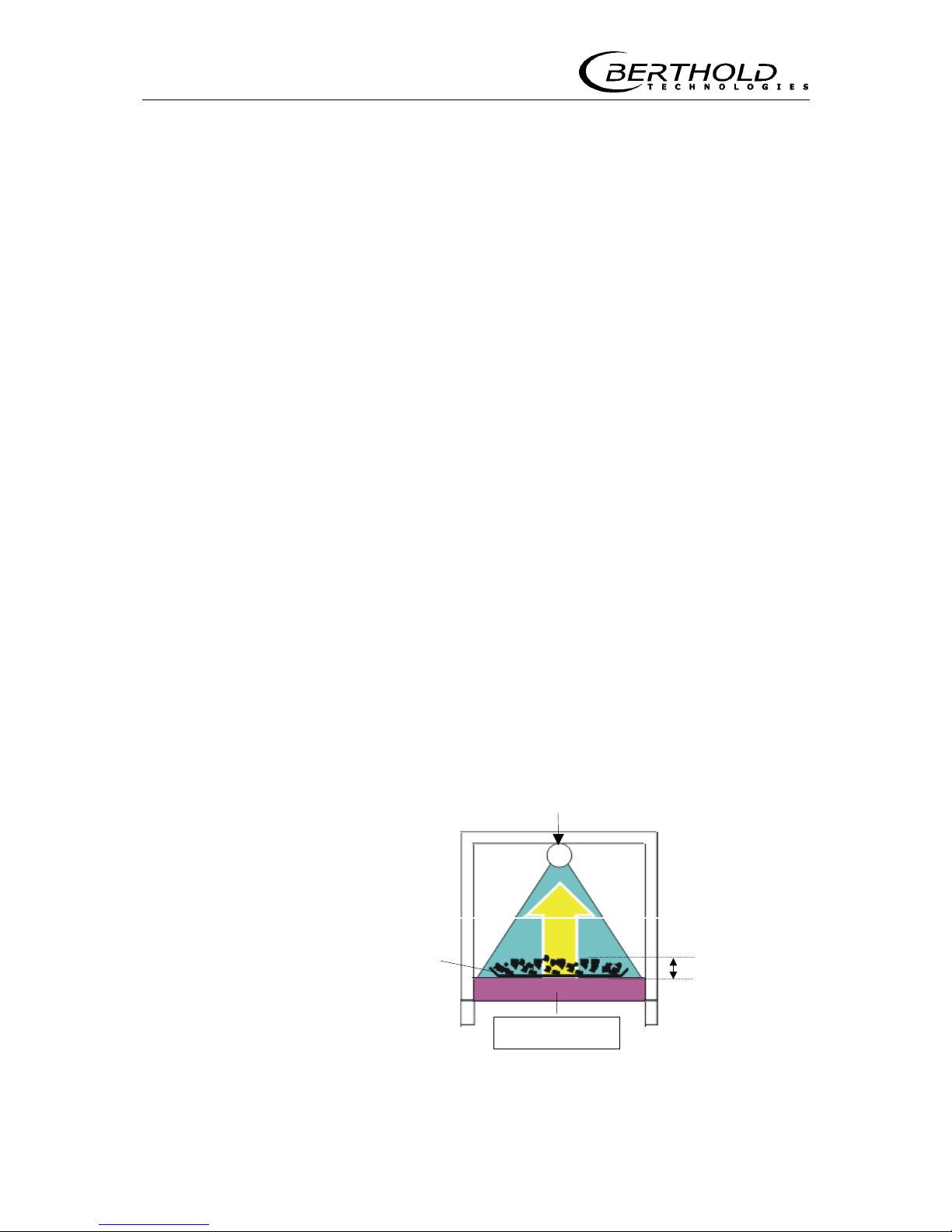
The principle of determining mass with a radiometric Bulk Flow Meter can be compared to that of X-raying material lying on the conveyor. To generate the radiation, which is physically identical to
that of X-ray radiation, radioactive material is used which is easy
to handle and whose energy is dependent on the load on the conveyor. The radiation is absorbed by the product on the belt and the
attenuated radiation is picked up by a detector and evaluated by
the microprocessor unit
The attenuation occurring during maximum conveyor throughput
determines the choice of source. Any material between source and
detector reduces the intensity to be measured at the detector.
The radiometric measurement utilizes the physical law of the attenuation of gamma radiation passing through the product being
measured. The resulting measurement effect is the ratio I/I0 between the unattenuated radiation I0 and the radiation I which is
attenuated by the product being measured. The remaining radiation picked up by the detector (scintillation counter) stands for the
mass of the product being measured. Figure 1 illustrates the principle of measurement. The radiation is attenuated according to the
following formula:
I = Io * e
- µ' * roh * d
I = Radiation picked up with load
I
0
= Unattenuated radiation without load
µ = Absorption coefficient) in cm
2
/g
roh = bulk density of the material on the conveyor in g/cm
3
d = height of absorbing material in cm
Detector
Figure 1: Principle of measurement
Source
ρ
d
Page 11

Section 2 System Description
9
The minus sign signifies that the intensity decreases as the load
increases. Apart from the constant factor, the initial intensity I
0
is
only affected by the product "roh
x d", where "roh" is the density
of the conveyed material, i.e. the bulk density, and d the path covered by the radiation in the material.
If we multiply "roh x d", we get the mass per unit of area. This
variable is known as the weight per area and is assigned the unit
g/cm
2
.
The intensity of the radiation is therefore dependent upon
the height and bulk density of the material. The product of
height and bulk density is the weight per area!
If the mass per unit of area is now multiplied by the material
width, the result is the mass over 1 m of the conveyor; multiplication by the speed results in the desired mass per time unit, e.g.
tons per hour.
Contamination of the product being measured or the pipeline wall
by gamma radiation is not possible at all.
2.3 Measuring Configuration
To be able to cover a certain measuring range continuously, a
measuring configuration must be realized where the dimensions of
source and detector form an optimum geometry covering a measuring field of equal size. The different options that are available
will be described below.
Which of these arrangements is chosen is dependent upon the
conveyor facility. Moreover, construction factors and customerspecific requirements may have an effect on the instrument selection. The respective selections are made during the planning stage
and have to be taken into account later during assembly and
commissioning.
A measuring system for the radiometric bulk flow measurement
typically comprises the following components:
a) Radioactive rod source inside a:
b) Shielding container with holding device for detector:
- Measuring frame with shielding container (conveyor belt,
etc.) or
- Holding device with shielding for free fall measurement
c) Detector
d) Evaluation unit LB 442
e) Two-wire cable
f) Tachometer (Option)
g) Cooling jacket for detector (option)
Page 12
2.3 Measuring Configuration
10
The power supply for the detector and the measuring signal
(pulses) are transmitted via the two-wire cable connected between
detector and evaluation unit.
Different configurations and mounting devices may be required,
depending on the conveyor system and the measuring tasks.
2.3.1 Configuration on Conveyor Belt
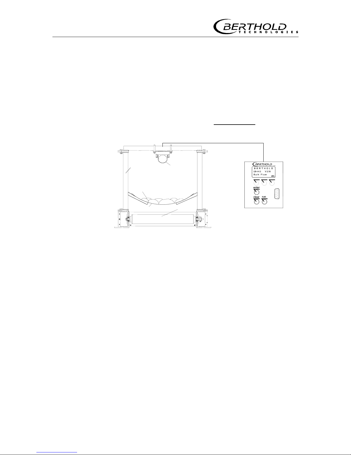
Figure 2 shows a basic setup on a conveyor belt. Basically, this
setup is the same for screw and chain conveyor types.
Measuri ng
Frame
Szintillation
Counter
Produc
t
Conve
y
or Bel
t
Rod Source
Figure 2: Measuring system mounted on conveyo r belt
The foot of the measuring frame contains the shielding container
with the rod source which is typically installed below the conveyor
belt.
The detector is mounted on the crossbeam of the measuring
frame, so that the detector opening is located directly above the
radiation exit channel of the shielding.
Detector and evaluation unit are connected via two-wire cable.
The optional tachometer is connected to the evaluation via 3-wire
cable.
See 13.5 Wiring Diagram in the Appendix on page 144.
Page 13
Section 2 System Description
11
2.3.2 Configuration for Free Fall Measurement
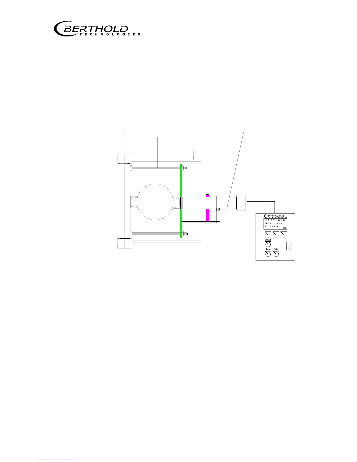
Using a clamping device, the radiation source (rod source) in its
shielding is installed on one side of the fall-pipe and the detector
on the opposite side. The radiation entrance window is located on
the front side of the detector.
with screw thread and protection plate
Shielding Bolt bar Shielding plate Detector
Figure 3: Top view of configuration for free measurement
Page 14

2.4 Instrument Description
12
2.4 Instrument Description
2.4.1 Rod Source
Radioactive sources for industrial applications are always „encapsulated radioactive substances“ which are tightly welded into a
sturdy stainless steel capsule, so that the radioactive substance
cannot leak out. Contamination is therefore ruled out. Moreover,
any activation of the product being measured by the sources used
is not possible for physical reasons.
The following rod-shaped Gamma sources can be used for these
measuring configurations:
241
Am, 60Co,
137
Cs, 85Kr.
The following isotopes are primarily used for the radiometric bulk
flow measurement:
a)
60
Co has a relatively high energy of 1.17 and 1.33 MeV, respec-
tively. It is used for very high loads. Its half-life period is 5.27
years.
*
b)
137
Cs is the isotope most frequently used for radiometric bulk
flow measurement. Its energy of 0.660 MeV is sufficient to irradiate common belt loads. Due to the lower energy, the measuring effect is better than with Co-60. Also, the shielding costs for
a Cs-137 source are lower than for a Co-60 source. The half-life
period of Cs-137 is approx. 30 years.
*
The rod-shaped Cs-137 source is assembled from several
pieces.
c)
241
Am has a very low energy (60 keV) which is much easier to
shield. Therefore, a much smaller lead shielding suffices. 241Am
is rarely used due to its minor radiation energy, mainly for materials such as tobacco and washing powder or for very low belt
loads.
Caution: Due to its low energy, it has to be borne in mind that
the attenuation of the radiation is dependent not only on the
bulk weight and height, but also on the atomic number. This
means that the result can be distorted when the chemical composition changes. How much has to be determined on an individual basis.
*
According to NBS, half-life is defined as: Time for the activity of
any particular radioisotope to be reduced to half its initial value.
Please note the Radiation Protection Guidelines in the
Service Instructions on page 89!
Page 15
Section 2 System Description
13
2.4.2 Measuring Frame for Conveyor Systems
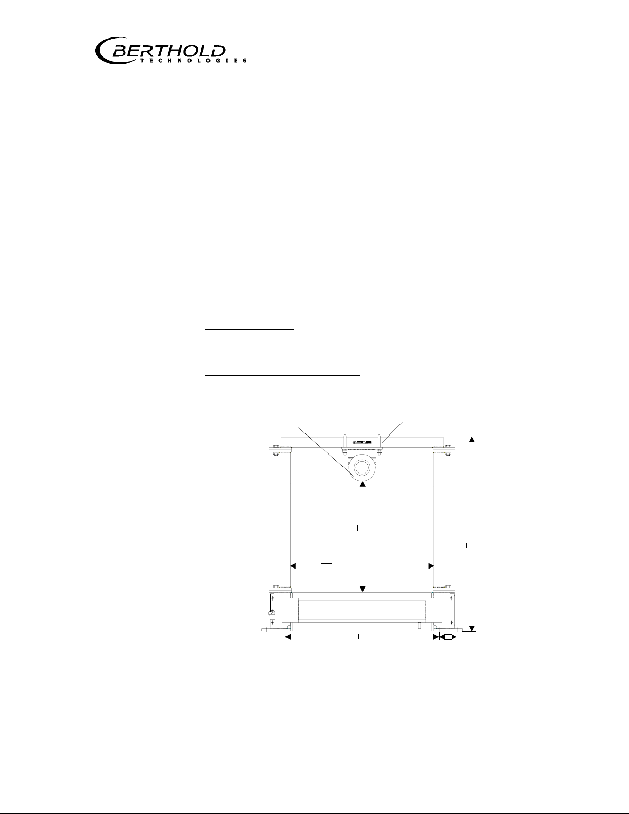
The measuring frame is a special construction for conveyor belts,
chain and screw conveyors; its foot includes the lead shielding for
the rod source. The detector is mounted to the crossbeam using
the supplied installation set. The product being measured flows between source and detector, with the source generally mounted below the stream of material to be conveyed.
Another frame installation is required for hot products if a heat
guiding plate or a water cooling protecting the detector cannot be
installed. For this application, the detector is mounted below and
the shielding with the source above the stream of material to be
conveyed.
There are two different types of measuring frames, the Cobalt/Cesium version and the Americium version.
Co or Cs version
: the detector is mounted horizontally using two
holding shackles below the crossbeam. Use the installation set enclosed with the instrument for installation.
Americium measuring frame
: the detector is installed vertically
using the clamping device attached in the center part.
Detector Detector holder
a
c
b
d
e
Figure 4: Measuring frame
Page 16
2.4 Instrument Description
14
Shielding
The effectiveness of the shielding and the smooth operation
of the lock must be checked every six months!
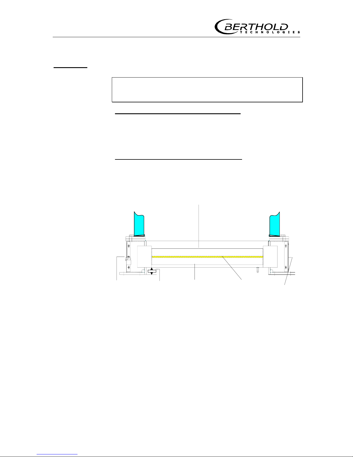
Measuring frames for Co and Cs sources are equipped with a
lead-filled steel pipe as shielding, the outer diameter being 105
mm, and a radiation exit channel having a width of 8 mm. When
the exit channel is closed, the radiation hits the steel shielding.
The open radiation exit channel is exactly aligned with the scintillation counter that is installed on the opposite side.
Measuring frames for Americium sources
do not require such
strict shielding precautions, since the radiation emitted by Americium is much easier to shield off.
Radiation exit channel
40 mm
Changing Distance from Shielding with rod source Opening/
the rod bottom 40 mm closing the
source radiation exit
channel
Figure 5: Shielding in foot of measuring frame
On one side of the shielding (see Figure 5) there is the opening for
changing the rod source which is secured by a special lock and a
padlock.
Page 17
Section 2 System Description
15
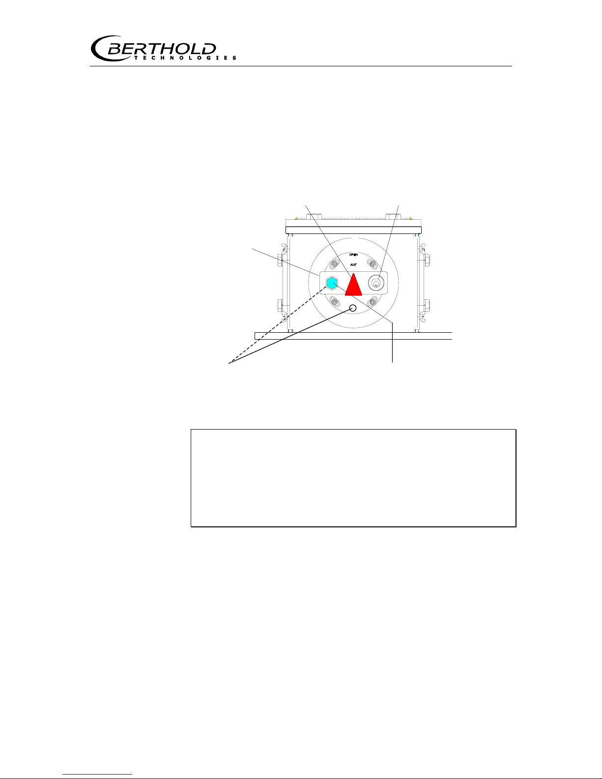
On the other side of the shielding is a device for opening and closing the radiation exit channel. To open or close the radiation exit
channel, turn the lever to the respective position (see Figure
6(a)).
The red arrow indicates the position of the radiation exit channel.
If it points up, the useful beam is opened toward the detector. If
this arrow points horizontally, the radiation exit channel of the
shielding is closed.
(e)
OPEN position (c) Lock
(d) Threaded - (b) Hexagon head cap screw
bore hole for arresting the shielding
Figure 6: Shielding (side view) in foot of measuring frame
Open radiation exit channel only for measurement operation!
Do not stay or reach into the radiation path!
With the radiation exit channel open, the hexagon head cap
screw must be tightened firmly!
Closing the radiation exit channel (see Figure 6)
1. Unscrew hexagon head cap screw (b) on metal plate (a).
2. Insert key in lock (c).
3. Push in lock and turn key to open the lock. Now you can move
the radiation exit channel by turning the lever (a).
4. Turn metal plate until the bore hole on the metal plate sits over
the next threaded bore hole (d). The red arrow (e) now points
horizontally.
5. Turn in hexagon head cap screw.
6. Turn key in lock and pull it out.
(a) Lever
for turning
the shielding
Page 18
2.4 Instrument Description
16
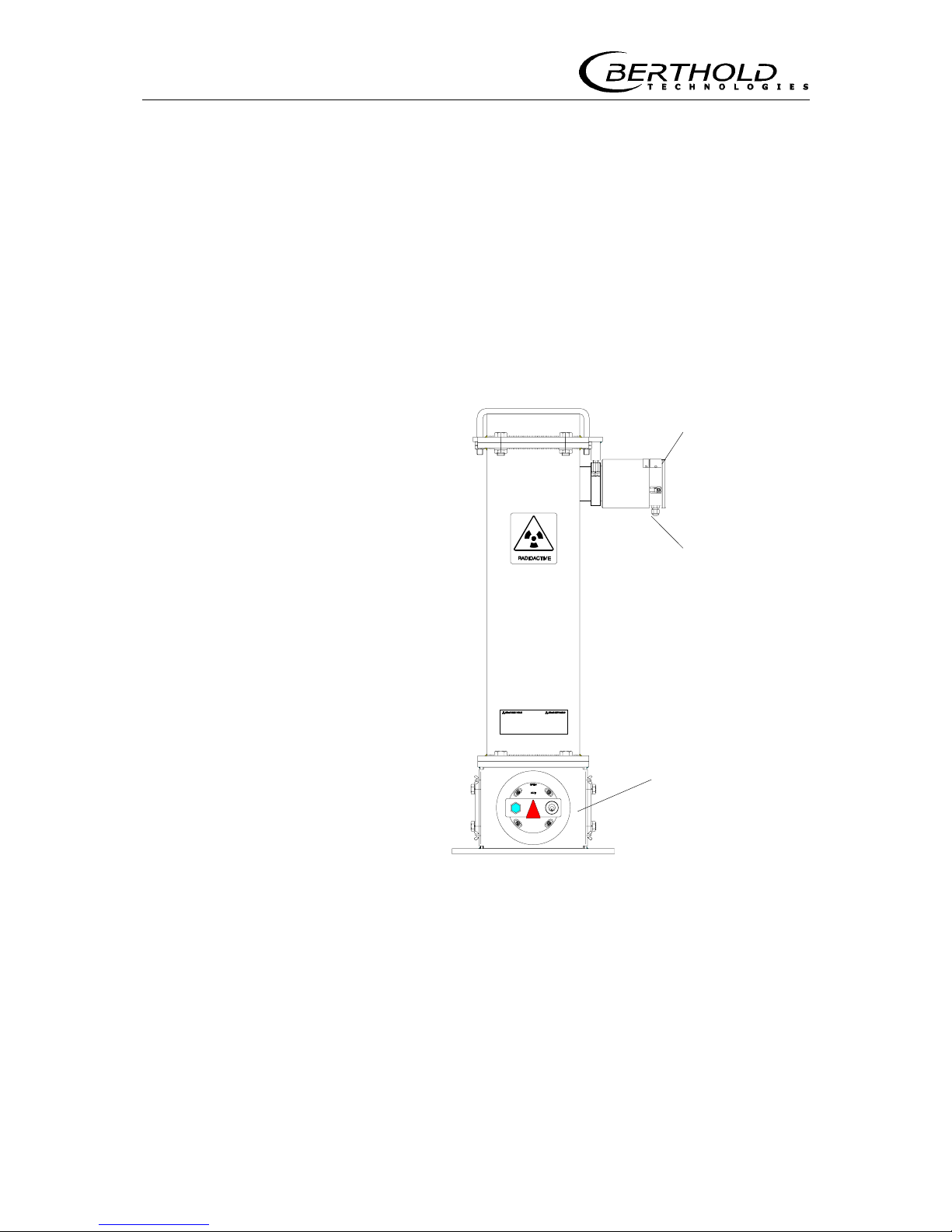
Opening the radiation exit channel (see Figure 6)
1. Unscrew hexagon head cap screw (b) at lever (a).
2. Insert key in lock (c).
3. Push in lock and turn key to open the lock. Now you can move
the radiation exit channel by turning the lever (a).
4. Turn lever until the arrow points straight up and the bore hole
on the metal plate sits over the respective threaded bore hole.
5. Turn in hexagon head cap screw and tighten it firmly (!). The
source must sit absolutely tight, so that possible vibrations of
the conveyor system cannot move the source in the shielding.
6. Turn key in lock and pull it out.
Figure 7: Measuring frame - side view
Detector
Connection to
evaluation unit
Shielding
Page 19
Section 2 System Description
17
2.4.3 Two-Detector Operation
Two detectors have to be used on wide troughed chain conveyor
systems, e.g. for measurements on recycling paper. The second
detector has to be connected to a special slave evaluation unit. The
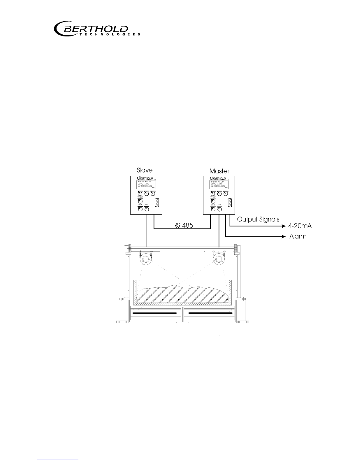
evaluation unit of the first detector works as a master. The count
rate and error messages of the slave system are transmitted to the
master via the RS 485 interface. See also the wiring diagrams on
pages 145 and 146.
Besides transmitting the count rates and possible error messages,
the slave has no further function. The master takes over control ofr
the entire measurement. Since both detectors are fully compatible,
it is irrelevant which of the detectors is connected to the slave or
to the master.
Figure 8: Master-slave wiring
With a 2-detector system, only the detector code has to be entered
at the slave.
See also Detector list on page 52 and Slave Menu on page 149.
Parameter setting and calibration are carried out on the Master. In
addition, the following parameter has to be set in the Master
menu, item Interface:
RS485: Slave
Number of detectors: 2
Page 20
2.4 Instrument Description
18
The Slave address in the Master can remain on the standard value
1, provided the standard address in the Slave has not been
changed.
See also Interfaces on page 65.
2.4.4 Measuring Device for Free Fall Measurement
The measuring frame must be installed close to the discharge station. This reduces the theoretical rate of fall at the measuring
point, for according to the law of gravitation the rate of fall rises as
the distance increases. With rising rate of fall the weight per area
and thus the accuracy of the measurement decreases.
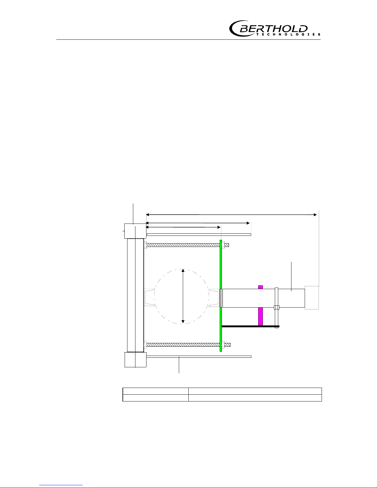
When using the free fall bulk flow meter on pipes, a measuring device as depicted in Figure 9 is used. The measuring device can
simply be mounted onto existing fall-pipes. It consists of a shielding with rod source and a variably adjustable holding plate for the
detector. Depending on the diameter of the fall-pipe, the holding
plate can be adjusted via the 4 threaded rods.
Am-241 shielding
Shielding plate preventing access to the radiation path
a = b = Variable adjustment
c = ca. 420 mm d = Pipe diameter between 89.9 and 304 mm
Figure 9: Free fall bulk flow measuring device (top view)
On fall chutes, measuring frame and rod source holder are used as
depicted in Figure 7.
a
b
c
d
Detector
Holding plate
Threaded rod
Fall-pipe
Page 21
Section 2 System Description
19
2.4.5 Measuring Frame for Rod Detector
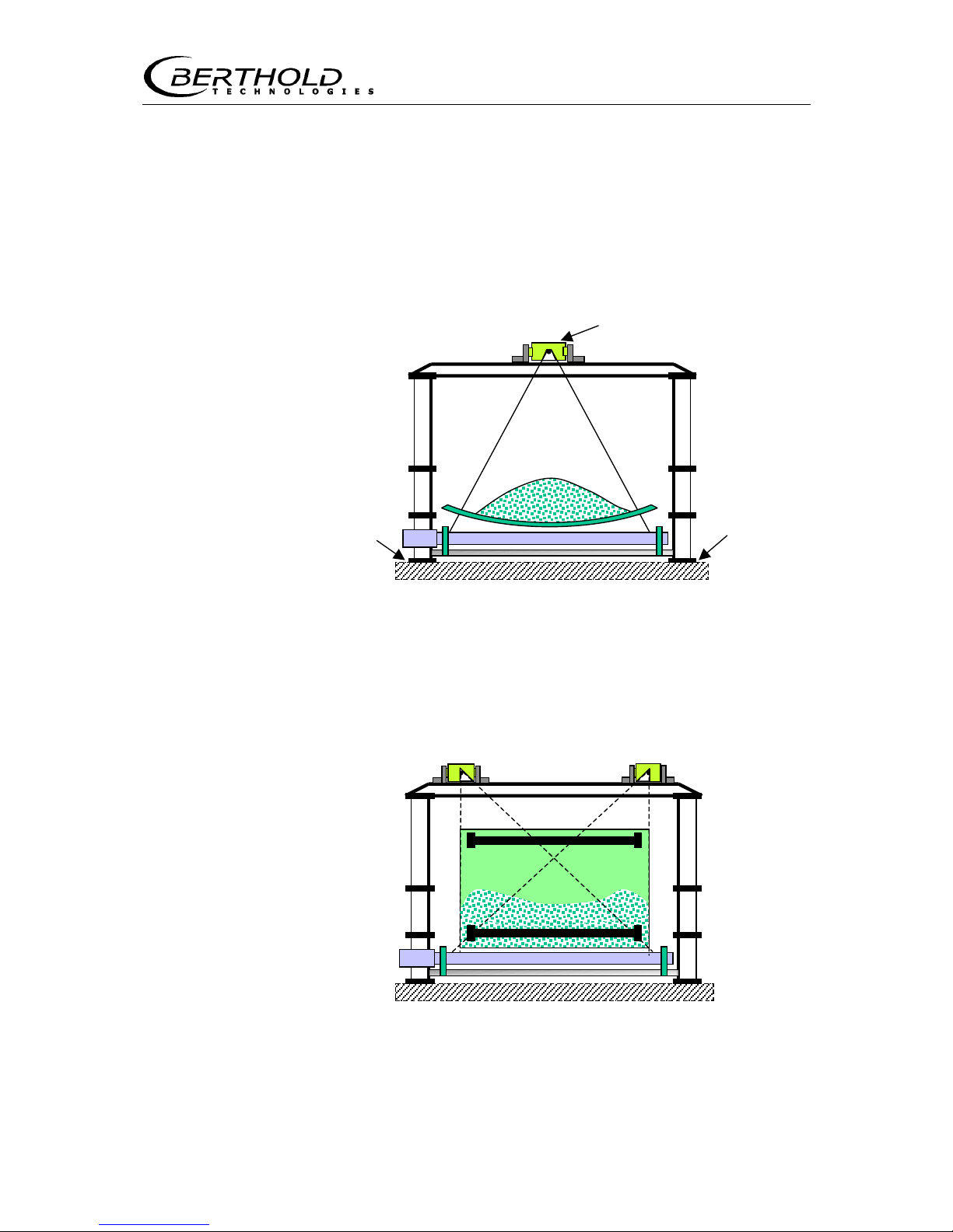
The measuring frame with rod detector works with a point source
or rod source. The principle of measurement is similar to that of
the point detector with rod source.
The measuring frame has to be fixed with screws at its foot ends
on a sturdy base.
Figure 10: Measuring frame for rod detector with one point source
If requested, rod detector and point source may also be installed
without measuring frame using a holding device provided by the
customer.
Two point sources may be used for measurement an a scraping
conveyor.
Figure 11: Measuring frame for rod detector with two point sources
Technical drawing for the rod detector and the measuring frame on
page 138 and 140.
Point
source shie
lding
Installation on
sturd
y
base
Installation on
sturdy base
Page 22
2.4 Instrument Description
20
2.4.6 Rod Source with Rod Detector
Rod sources with rod detectors allows measurement at very low
source activities and can be used for wide conveyor systems.
2.4.7 Point Source Shielding
Depending on the activity or isotope, we distinguish between three
different shielding sizes. Each of these shieldings offers radiation
exit angles of 54° and 72°. Selection of the exit angle is dependent
on the measurement geometry.
See drawing for Point Source Shielding on page 142.
2.4.8 Detector
Scintillation counters are used as detectors, since only these detectors provide the required high sensitivity to Gamma radiation and
their service life is not limited by the radiation field.
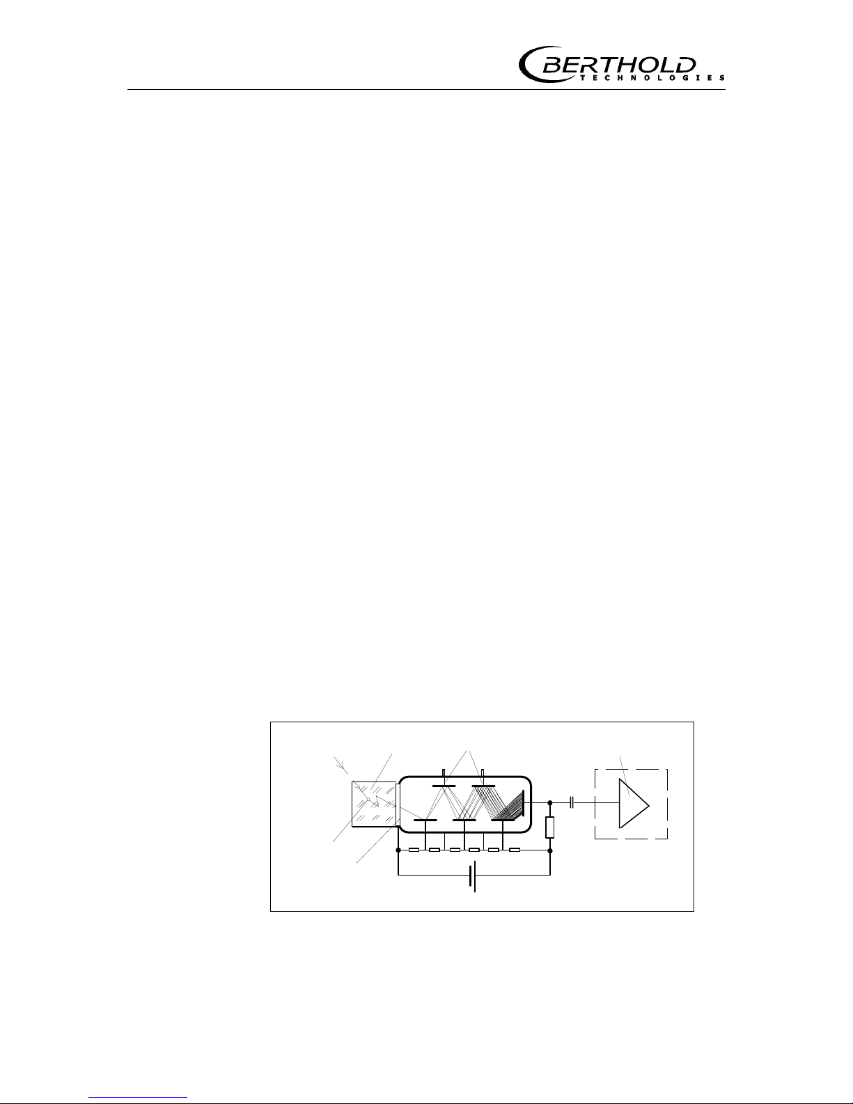
The detector comprises
a) sodium iodide crystal doped with Thallium
b) photomultiplier
c) electronics unit.
The built-in microprocessor defines the configuration, counts the
pulse rates, controls the high voltage, measures the temperature
of the probe, transfers data and performs calibration and control
functions. Supply and communication with the evaluation unit LB
442 take place via two-wire cable.
The detector material consists of a special crystal which generates
flashes of light when absorbing Gamma radiation. The number of
light flashes per unit of time is a measure for the intensity of the
measured radiation field. The individual flashes of light are very
short, so that a high resolution is achieved and this detector can be
used for high count rates.
+
−
AmplifierRadiation
Light flash
Scintillator Dynodes
Photo cathode
.
.
.
Figure 12: Scintillation counter
Page 23

Section 2 System Description
21
These flashes of light are detected by the light-sensitive layer of a
photomultiplier. Electrons released from this layer are then moved
to several dynodes by means of high voltage cascade to release
further electrons there. During this process virtually every electron
triggers an electron avalanche. The pulses created in this manner
are counted in the detector and the results transmitted to the
evaluation unit LB 442. A photomultiplier which is optically coupled
to the detector converts the flashes of light into electrical signals.
To achieve a very high accuracy and high long-term stability, the
integrated processor automatically adjusts the optimum operation
point of the photomultiplier, monitors the limit values, and stores
all detector-specific data. Power is supplied via 2-wire technique;
all measured data and information can be transmitted between detector and evaluation at the same time.
The detector is assembled in a sturdy stainless steel housing which
protects the instrument against normal environmental stress.
To ensure reliable function and a long service life, the detector must not be subject to heavy mechanical stress and vibrations.
The ambient temperatures must not exceed 50°C; otherwise, adequate cooling has to be provided either by:
installing a cooling jacket (see section Installation of Water
Cooling) installing a shielding plate if the detector is exposed to sunlight.
The det ector for the Cobalt/Cesium version
is mounted on the
measuring frame parallel to the conveyor, since the sidewalls and
the centerpiece of the measuring frame absorb a major share of
the radiation.
The opening of the detector must be exactly vertical above the
source.
The detector for the Am version
is mounted vertically to the
conveyor.
Page 24

2.4 Instrument Description
22
2.4.9 Tachometer
The tachometer is used to measure the conveyor speed. It is supplied with power by a separate power supply unit. The evaluation
unit LB 442 can process signals from pulsed tachometers with 500
pulses/rev or 5000 pulses/rev as well as current signals (0/4 - 20
mA) proportional to the speed.
For measurements on a conveyor belt, a running wheel having a
diameter of 160 mm is attached to the tachometer. In this case,
the tachometer including the flexible holder has to be installed in
such a manner that the wheel is running on the lower belt.
For measurements on chain and screw conveyors, the tachometer is attached to a rotating axle via a flexible coupling. The driving
axle should have a diameter of 12 mm.
Provided the conveyor speed is constant, the speed need not be
monitored on-line. Several experiments and statements by manufacturers of conveyor systems show, however, that the speed is
not constant immediately after starting the conveyor.
See also information on Tachometer Installation in the Appendix
on page 130.
Page 25
Section 3 Installation
23
Section 3 Installation
3.1 General Safety Precautions
The shielding with the radioactive source is delivered in a box in
compliance with the regulations concerning transportation of radioactive substances.
Take the shielding out of the box just prior to installation.
Up to that time, store it in a location that is guarded against
unauthorized access.
Using the drawings of the shielding and taking into account the
situation at the measuring site, carefully install the mounting
brackets and fixings. Make sure that the mechanical stability of the
mounting devices matches the weight of the shielding. The shielding should be assembled just prior to taking the system into operation.
Secure all screws and fixing parts, so that they cannot come
undone during operation, and the shielding cannot fall
down.
To keep the radiation exposure of the assembling personnel as low
as possible, only licensed personnel who have been trained on how
to handle radioactive substances are allowed to assemble or disassemble the shielding with the source.
The work is performed according to the instructions and under the
supervision of the Radiation Safety Officer. It has to be ensured
that the lock of the shielding is closed and secured, so that no unshielded radiation can exit. Make sure the shielding is not modified
or damaged.
Very important! Please read the Radiation Protection Guidelines in Section 12 Radiation Protection and observe them
exactly!
The radiation exit channel must always be closed during installation!
Page 26
3.2 Installation of the Measuring Device
24
3.2 Installation of the Measuring Device
The detector must be protected against temperatures
> 50°C by a water cooling jacket.
The cables must be protected against temperatures > 70°.
In case of outdoor installation, the detector has to be protected against sunlight by installing a guard plate.
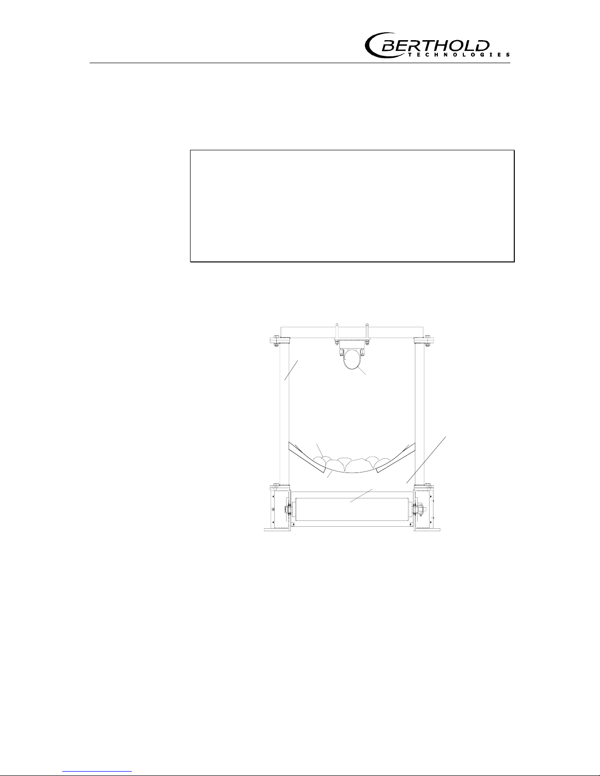
3.2.1 Installation on Conveyor Belts
Meßbügel
Szintillationsdetektor
Schüttgut
Förderband Stabstrahler
Figure 13: Installation of measuring device on conveyor belt
General information on how to install a measuring frame
□ The measuring frame is constructed such that the shield-
ing with source is located below and the detector above
the conveyor belt.
□ The distance between the lower edge of the upper belt
and the upper edge of the source shielding should be
approx. 10 mm. This means that the shielding is to be
mounted between two rollers.
Shielding
Measuring
frame
Bulk good
Conveyor belt
Rod source
Scintillation
detector
Page 27
Section 3 Installation
25
□ If very hot material is being conveyed, a heat conducting
tin plate must be installed between the conveyor flow
and the detector. On request, a water cooling jacket can
be supplied for the detector. A different frame assembly
is required if the insulation or the water cooling system
cannot be installed. In this case, the detector has to be
installed below and the shielding including the source
above the conveyor flow.
□ The measuring frame is to be mounted such that
- there is sufficient space in front of the lock to replace
the source (about 2 m)
- that the other side of the measuring frame is easily
accessible to open/close the radiation exit channel.
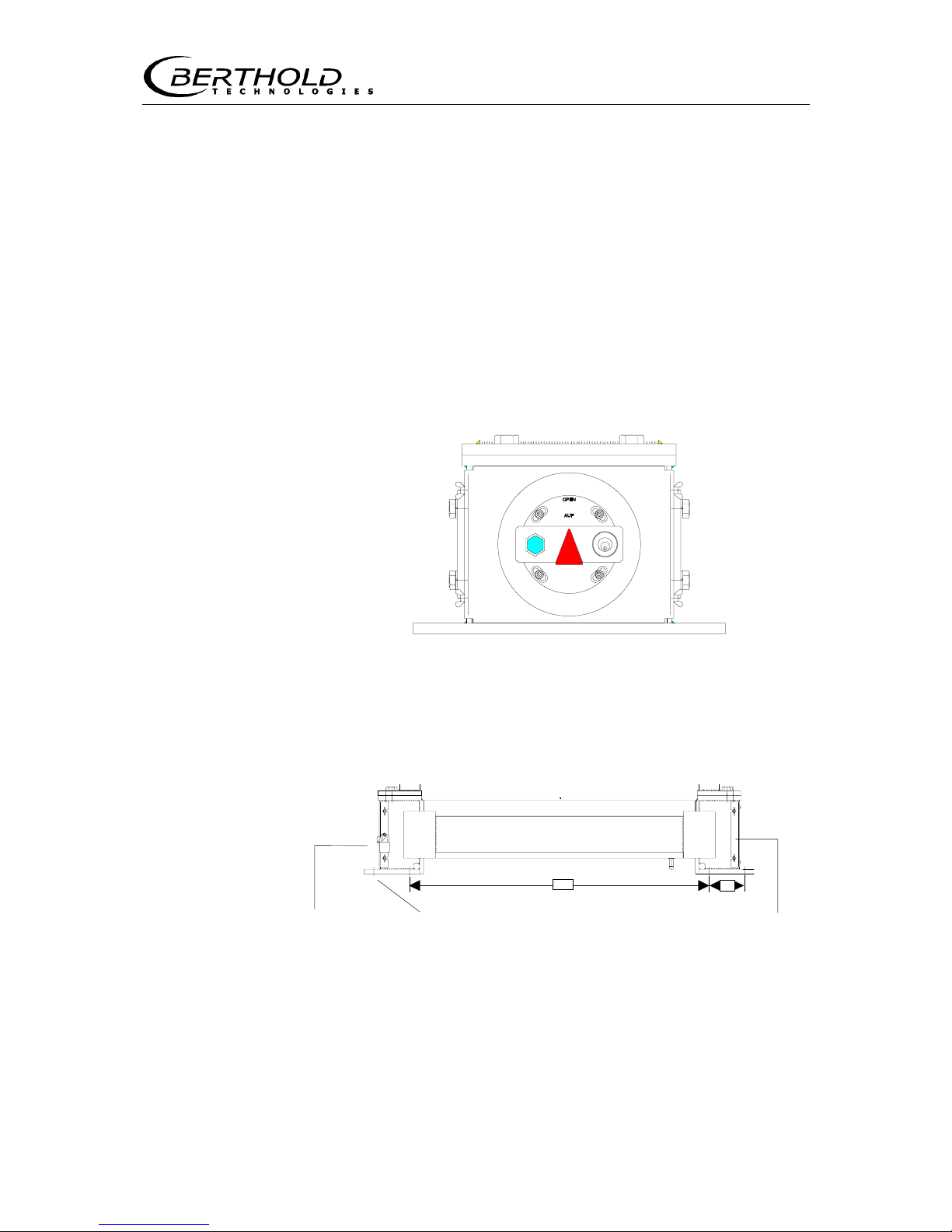
Figure 14: Rotating lock for opening/closing the radiation exit
channel
a
b
Changing the Bottom plate Opening/closing the
rod sources see Figure 16 radiation exit channel
Figure 15: Measuring frame foot with shie lding
Position
OPEN
Page 28
3.2 Installation of the Measuring Device
26
Procedure:
A) Installation of Measuring Frame
See also the Mechanical Drawings on page 133
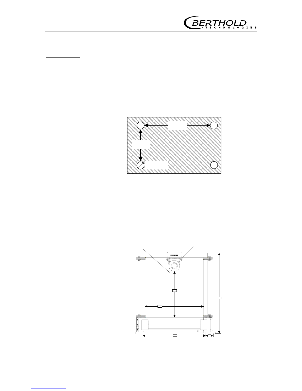
□ The measuring frame has to be split up into two parts,
the foot with the shielding (Figure 14) and the top part,
consisting of the two verticals and the crossbeam
Figure 16: Bottom plate of measuring frame foot
□ Base and bore holes (Figure 16) for installation of the
measuring frame foot at a suitable site according to the
dimensions below the conveyor belt and in a suitable
height.
□ Insert measuring frame foot and fix it.
□ Screw top part of measuring frame onto foot.
Detector Detector holder
a
c
b
d
e
Figure 17: Measuring frame
300m
90mm
Page 29

Section 3 Installation
27
B) Mounting the Detector
Co or Cs measuring frames
□ Dismantle the mounting set enclosed with the instru-
ment.
□ Fix the detector to the holding plate using the clamps
and the hexagon head cap screws.
□ Fix holding plate using the two fastening bows in the
center of the top part of the measuring frame. The window of the detector head must face the source and be
located vertically above the source. The window is adjusted correctly if it is in the dead center of the measuring frame.
Americium measuring frame
□ The detector is fixed to the Americium measuring frame
using the clamping device attached to the centerpiece.
□ The detector is installed properly if it extends about
75 mm beyond the frame measured from the lower edge
of the centerpiece.
□ Readjust the detector after you have connected and
turned on the evaluation unit and opened the radiation
exit channel: The highest count rate is displayed in the
correct position (see section Re-adjusting the Detector).
3.2.2 Measuring Frames on Screw Conveyors
The same instructions apply for the installation of measuring frame
and detector on a screw conveyor.
The measuring frame should be installed in a location where the
material in the screw conveyor flows smoothly. This means that
the conveyor material in the screw conveyor must not fall back behind the screw shaft, as otherwise the material speed cannot be
measured accurately. The material flow can be optimized by increasing the conveyor throughput speed.
Page 30
3.2 Installation of the Measuring Device
28
3.2.3 Measuring Frames on Chain Conveyors
The same instructions also apply for installation on a chain conveyor system. The bottom part of the measuring frame must be
mounted as closely as possible to the chain conveyor.
With this installation, however, one has to make sure that the installation angle, which is determined at the planning stage, will be
realized. Due to this installation angle, irradiation of a scraper
while the conveyor is moving will be reduced to a small section. As
a result, one will get a smoother output signal.
3.2.4 Installation for Free Fall Measurement
Install measuring frame close to discharge station!
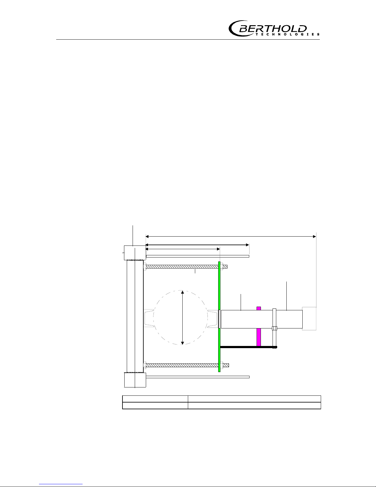
When using the free fall bulk flow meter on pipes, a measuring device as depicted in Figure 20 is used. The measuring device can
simply be mounted on existing fall-pipes and adjusted via the 4
threaded rods.
Shielding
a = b = Variable adjustment
c = ca. 420 mm d = Pipe diameter between 89.9 and 304 mm
Figure 18: Free fall bulk flow measuring device (top view)
a
b
c
d
Detector
Holding
Threaded rod
Fall-pipe
Page 31
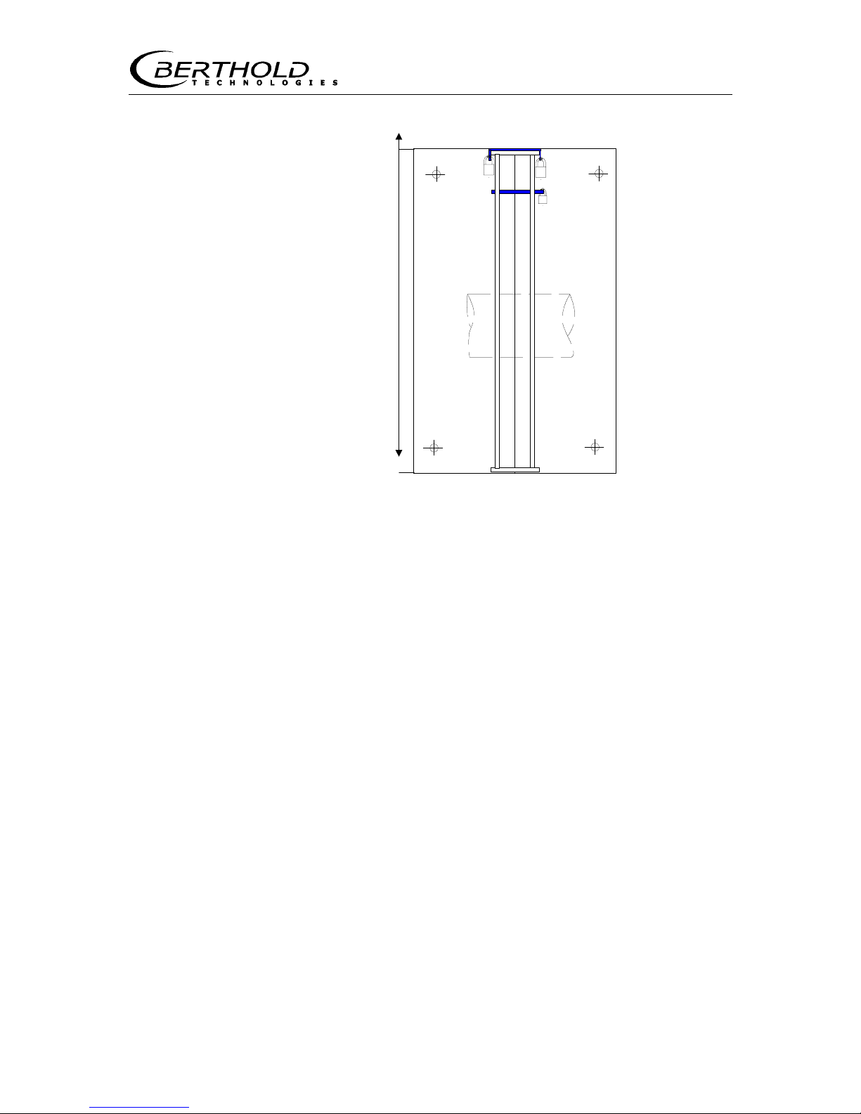
Section 3 Installation
29
Figure 19: Free fall bulk flow measuring device (side view)
On fall chutes, measuring frame and rod source holder are used as
depicted in Figure 17.
approx.
484 mm
Page 32
3.3 Installation of Water Cooling
30
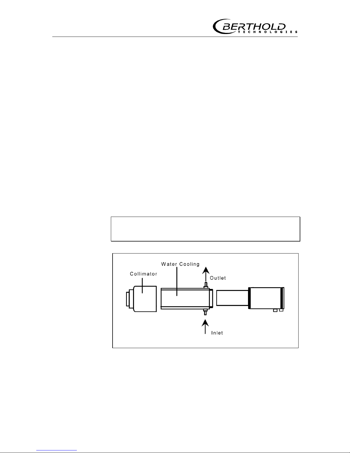
3.3 Installation of Water Cooling
The maximum operating temperature of a scintillation
counter is 50°C. A cooling system (which is available as extra)
must be used if the temperature at the detector is likely to be
higher, due to heat emission of the pipeline and/or higher ambient
temperatures.
The detectors LB 44.. permit later installation of this cooling
jacket. With the scintillation counters LB 5... the cooling jacket is
installed in such a manner that the connection studs are located on
the side of the connection box, so that they can simply be fixed
with the clamping device.
Installation on the scintillation counters is done in the same manner. First, however, the lead shielding at the front has to be removed, and also the distance ring. After sliding over the cooling
jacket, screw the lead shielding on again without distance ring.
The water must enter from below and exit at the top. Thus,
the cooling jacket is always filled with water, ensuring good thermal insulation.
In case of higher ambient temperatures, the connection cables used have to be able to withstand these temperatures!
Figure 20: Installation of water cooling
Page 33
Section 3 Installation
31
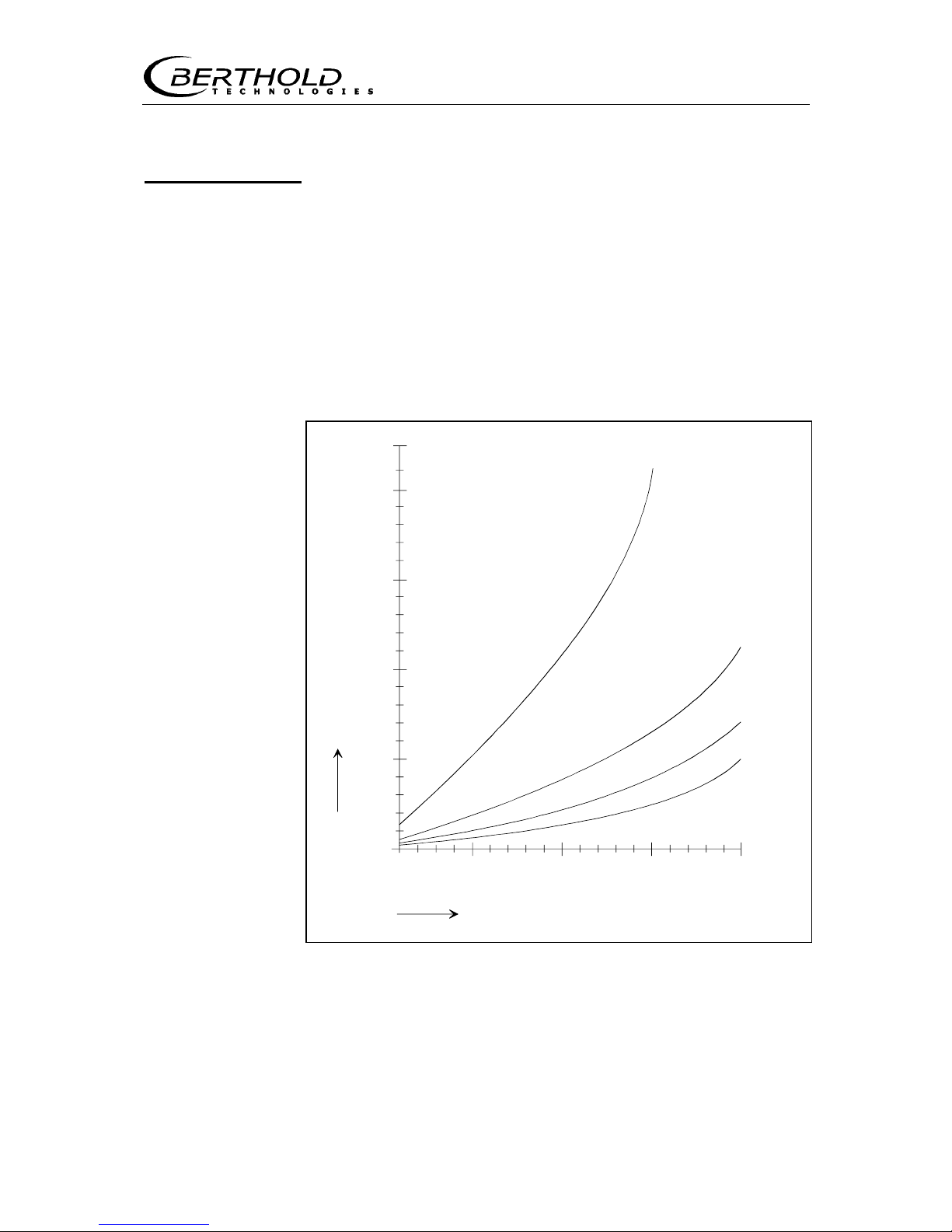
Cooling Medium
Water should preferably be used as cooling medium, because air
does not ensure adequate cooling at high temperatures. The water
must be clean to avoid dirt deposits in the cooling jacket which
would have an adverse effect on the cooling efficiency.
The diagram below shows the quantity of cooling water required
for the detectors LB 44... The ambient temperature was taken into
consideration when calculating the required quantities, but not any
possible heat emission by surrounding components, e.g. containers, pipelines, etc. If this is the case, a higher rate of cooling water
may be required.
10
40°C
30°C
20°C
10°C
Ambient detector temperature °C
Water flow rate for scintillation counter
Inlet water temperature in °C
Flow rate l/h
max. pressure 6 kg/cm
2
50
100
150
200
220
60 80 100 150 200
Figure 21: Required amount of water cooling
Page 34

3.4 Tachometer Installation (Option)
32
3.4 Tachometer Installation (Option)
3.4.1 Conveyor Belt Installation
The tachometer measuring the speed of the conveyor belt is
equipped with a flexible holder and a running wheel. Install the tachometer such that the wheel is running on the lower belt. Two
threaded rods size M 12 are fixed to the holder. Both screw threads
are 65 mm apart (see dimensional drawing no. 4507, 105 in the
Appendix).
3.4.2 Chain and Screw Conveyor Installation
The tachometer measuring the speed of chain or screw conveyors
is equipped with a flexible coupling. The coupling is fixed to an
axle having an outer diameter of 12 mm. The coupling is 50 mm
long and the outer diameter 26 mm. For tachometer with fastening
bore hole and coupling see drawing no. 4507. 106-000 in the Appendix.
3.5 Installation of Evaluation Unit
When installing the evaluation unit, please keep in mind:
a) According to the Ex protection criteria, the evaluation unit must
only be used outside the Ex-area. If the evaluation unit detector system is used in accordance with inherently safe criteria, an equipotential bonding has to be established between
detector and evaluation unit.
b) Please note the maximum cable lengths between evaluation unit
and detector. See section Technical Data.
c) The evaluation unit should not be installed outdoors.
Other than that, installation of the evaluation unit is simple, since
the frame is designed in 19“ technique and two bore holes each
are foreseen at both butt straps to which the unit can be fixed at
the protective housing. To do this, open the front door of the protective housing and you will see 4 lead-screw nuts. The respective
screws for fastening are enclosed. Installation in a control cabinet
is done in the same manner.
Page 35
Section 4 Electrical Connections
33
Section 4 Electrical Connections
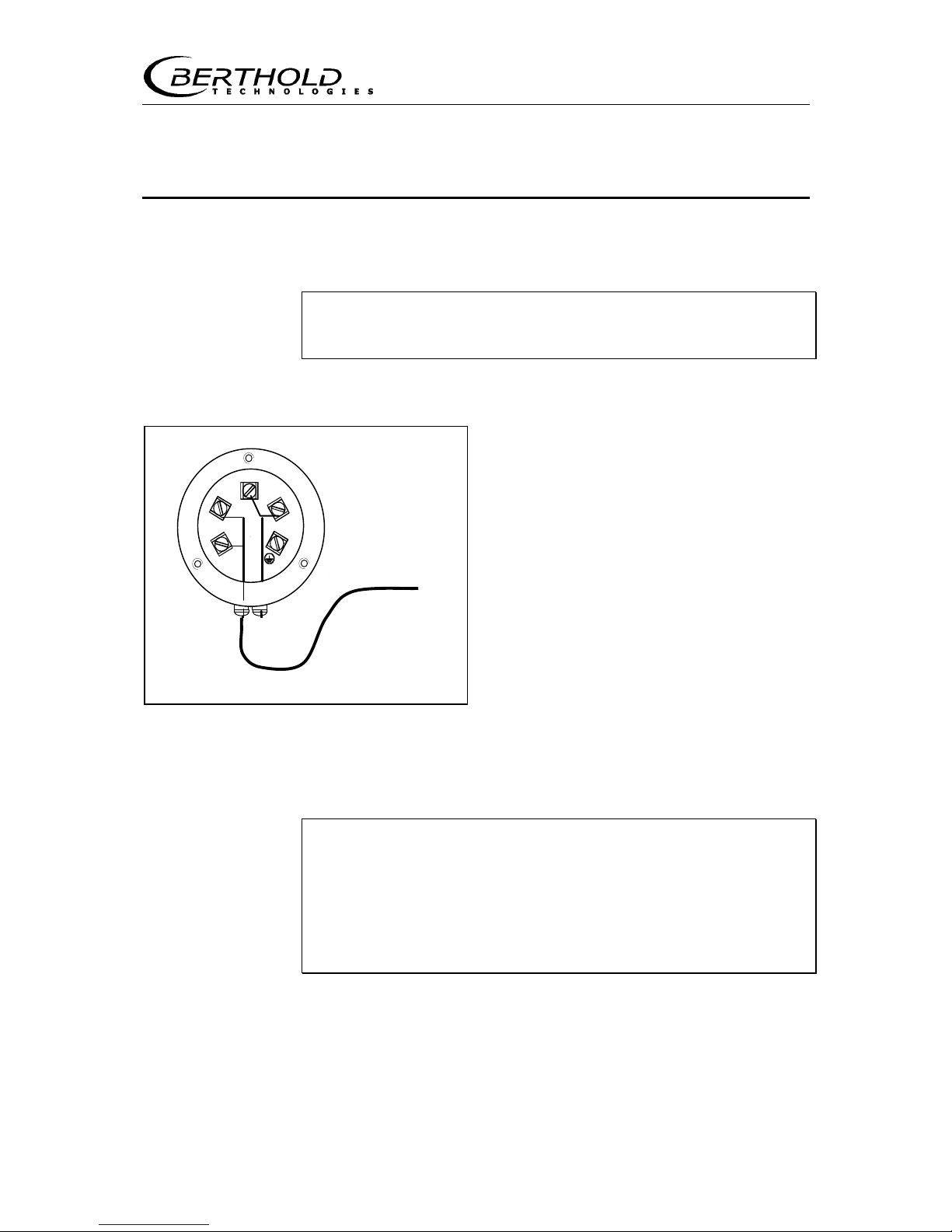
4.1 Detector
Switch evaluation unit off before connecting the scintillation
counter.
Open the screws and remove the connection box cover to expose
the connection area.
The detector is connected to terminals 1
and 2 on the evaluation unit via a 2-wire
(2 x 1 mm
2
) shielded standard cable with
6 mm diameter. This cross-section allows
a maximum length of 750 m. When installing the connection cable, you have to
make sure that water cannot get into the
connection room via the cable. With ambient temperatures >70°C, the installed
cable has to be protected to prevent exceeding of the temperature limits of the
cable. Following connection, check that
the connection room is carefully closed
and the cable bushing properly sealed.
With a rod detector, a 6 m longer cable
has to be connected to determine the
background.
See also page 68 "Background".
Figure 22: Cable connections at detector
For equipment installed in the Ex-area, please observe the
special requirements for the cable and the preparation of
the connection wires.
The detector LB 44... has to be used for installation in the
Ex-area.
The evaluation unit must always be installed outside the Exarea.
A special transmission technique ensures that interference will be
suppressed. Nevertheless, the cable should not be installed together with power cables.
1
2
3
4
5
Connections
in detector
to evaluation
unit LB 442
Page 36
4.2 Evaluation Unit LB 442
34
4.2 Evaluation Unit LB 442
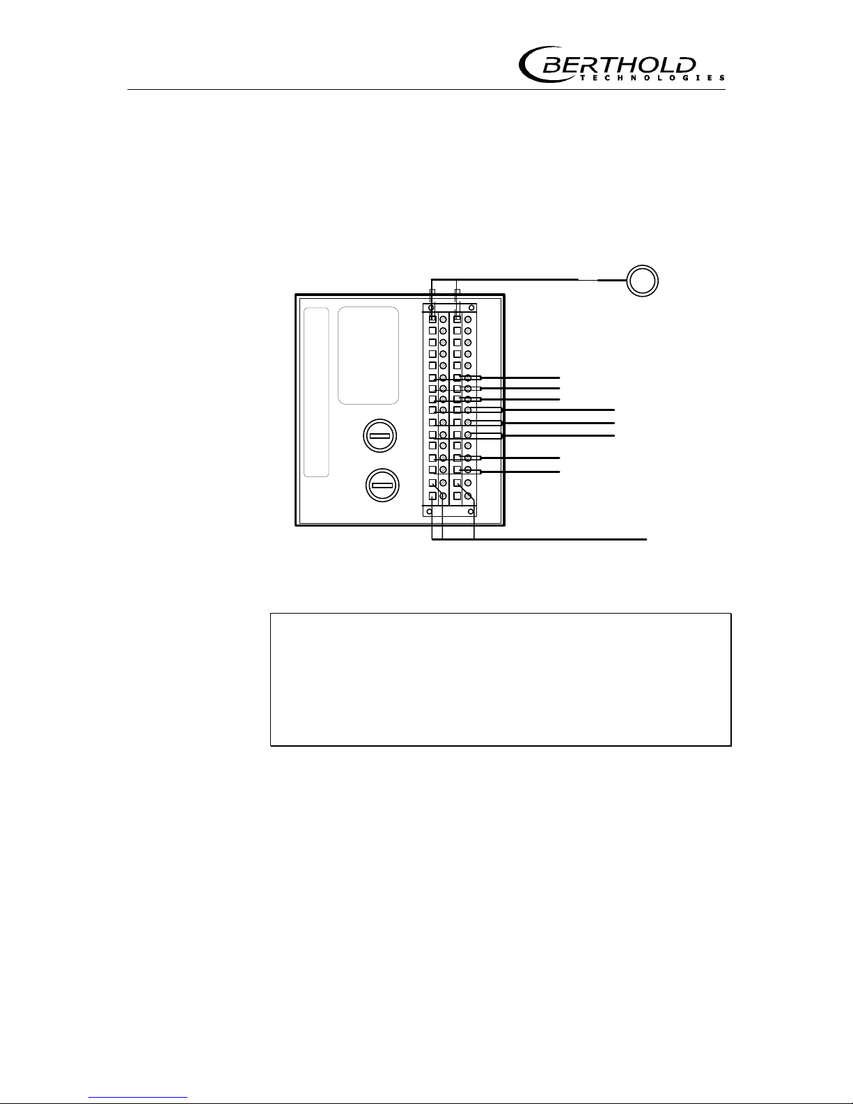
Make the connections on the rear panel of the evaluation unit as
shown in the wiring diagram in the appendix to this manual on
page 146.
LB 442
Detector
Mains supply
Fuse
ca
2
4
6
8
10
12
14
16
18
20
22
24
26
28
30
32
Relay 1
Relay 2
Relay 3
Dig. In 2
Dig. In 3
Current In (+/-)
Current Out (-/+)
1(+)
2(-)
Voltage
selector
Dig. In 1
Figure 23: Terminal connection evaluation unit (rear panel)
Carefully note the power supply for the instrument and observe all safety previsions regarding the power supply.
A separate fuse protection and an easy to access shutoff
have to be foreseen, since the evaluation unit does not include its own mains switch.
Refer to the wiring diagram in the appendix to this manual for the
connections. The terminals are described as follows:
Detector Terminal (2a/2c)
Connection is made via 2-wire technique; the detector protection
type is EEx de IIC T6 or EEx de (ib) IIC T6 or EEx de (ib) IIB T6.
For inherently safe installation, the cable ends on the strip terminal
must be protected by a 10 mm long shrink-down plastic tubing
(see also the connection diagram).
Page 37

Section 4 Electrical Connections
35
Terminals for Relay 2 (12a/12c)
o Mass Counter
Output active when the relay picks up. The relay supplies pulses
(25 ms long) for external electronic
mass counter.
Terminals Relay 3 (14a/14c)
o Tare measurement
o Batch Ready
o Min/Max
Output active when the relay picks up. Depending on the software
configuration, the relay can be used for signaling Tare measure-
ment, Batch Ready or Min/Max.
- Tare measurement :
Relay is energized during tare measurement and the contact is
closed. During tare measurement, RUN appears on the display.
- Batch Ready:
Relay picks up when batch weight is reached. Measurement is
stopped.
- Min/Max:
You can select in the software if the relay picks up when dropping
below (Min) or exceeding (Max) the selected load. Hysteresis adjustable.
Connections relay 1 (16a/16c)
o Error alarm
Output active when relay is idle. The relay signals an error.
Digital input 1 (18a/18c)
o Belt stop
o Erase ext. batch
o Batch mode
- Belt stop
With closed contact the measurement is stopped and the last
measured value is held. This function can be used only at constant
belt speed.
- Erase mass integrator
If the input is short-circuited, the mass integrator is reset to 0 t.
(Only in continuous mode).
Page 38
4.2 Evaluation Unit LB 442
36
- Ext. batch measurement start
Start of external batch measurement. Relay 3 must also be set as
Batch Ready.
Start
The measurement starts when the contact is closed. The mass
counter starts at 0 t. Contact of relay 3 is open.
Stop
The measurement stops as soon as the specified batch weight is
reached. Contact of relay 3 is closed. The batch weight obtained is
held until the next start.
Digital input 2 (20a/20c):
o External Tare
o Prin t s ta rt
o External pr oduct 3+4
o Start / Stop and print
Input active when terminals are short-circuited.
See also Digital input 2 page 56
- External Tare:
Automatically starts a tare measurement (also in regular measurement operation and saves the result).
- Print start
The actual tonnage is output to the printer. The print row corresponds to a row of the minute printout.
- Product 3+4
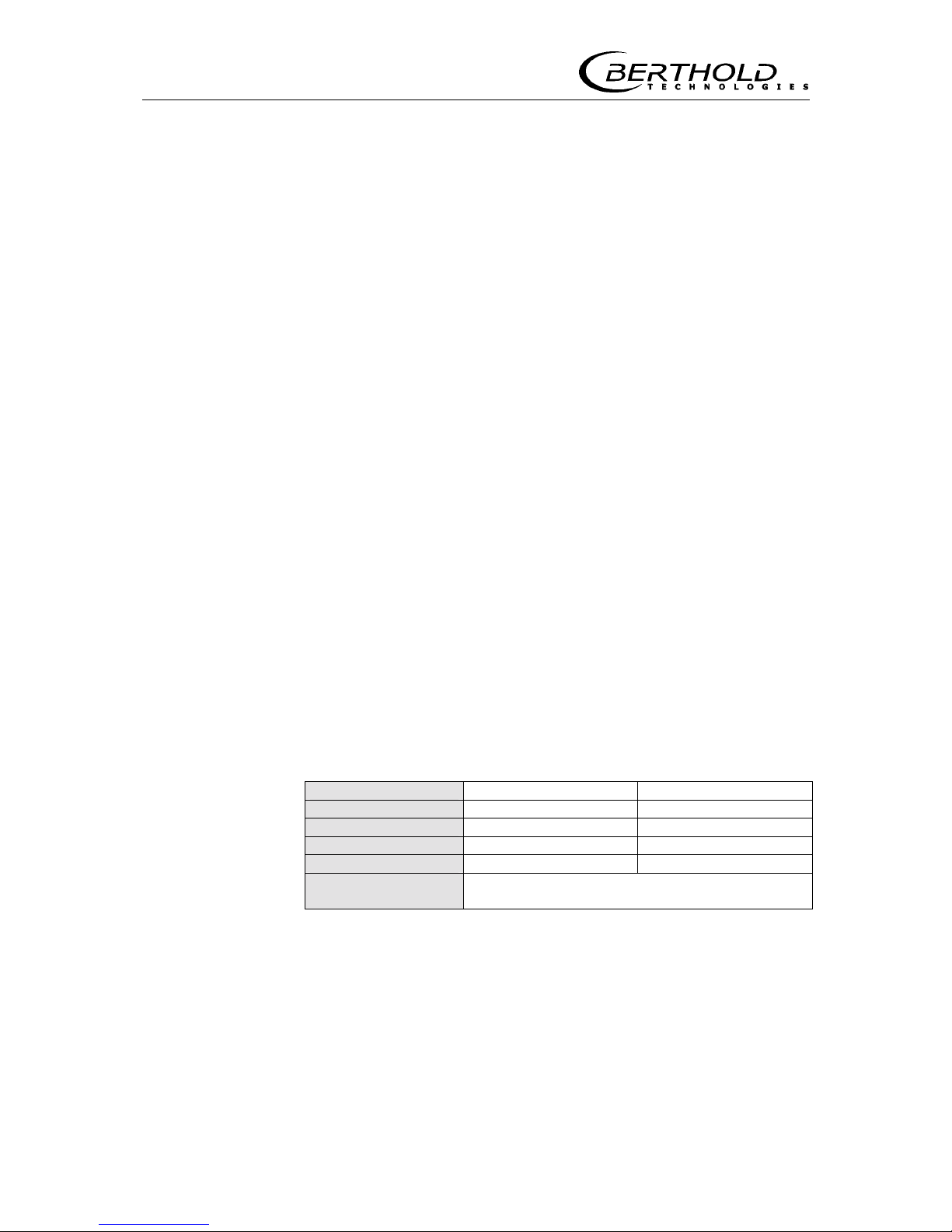
Digital input 2 can also be used to expand the external product selection. In this case, different products can be selected as shown in
the table below:
Menu Dig. input 2 Dig. input 3
1 0 0
2 0 1
3 1 0
4 1 1
1 = closed contact
0 = open contact
Table for external product selection 3+4
- Start/Stop and print
If the contact is closed, a tare measurement is carried out first.
Then the measurement automatically changes over to the measurement mode. The measurement mode is interrupted as soon as
the contact is opened. After the measurement, a printout is created automatically, including date, time and measured tonnage.
Page 39
Section 4 Electrical Connections
37
Digital input 3 (22a/22c)
o Product selection
Input active, when terminals are short-circuited.
Terminal open means product 1
Terminal closed means product 2.
If digital input 2 has been selected for function "Pr oduct 3+4 ",
the "Table for 4 products" is valid.
See also page 36 Digital input 2
Current output 0/4-20mA (26a+/26c-)
o Load
Insulated current output.
Current input (28a-/28c+)
o Pulse input
o Speed or Moisture
Depending on the configuration selected in the software, either
current signals or pulses supplied by a tachometer or a moisture
signal (0/4 - 20 mA) can be fed.
RS 232
Terminal for data transfer from evaluation units to printer or PC
(front panel of evaluation unit).
Power Supply (30a/30c)
Power supply 115V/230V or 24 VAC or DC, depending on power
supply unit (see label on instrument rear panel!).
Fuses
To replace fuses, you have to open the turn-lock using a coin.
Note the fuse type and power!
Observe type and power of fuses!
Before turning on the power supply, carefully check all connections once more to rule out any damage to the instruments.
Page 40

5.1 Quick Installation Overview
38
Section 5 Getting Started
5.1 Quick Installation Overview
1. Observe safety instructions
23
2. Install measuring system
: 24
measuring frame with shielding and detector
on conveyor belts 24
on screw conveyors 27
on chain conveyors 28
device for free fall measurement 28
3. Install water cooling
for temperatures >50°C 30
4. Option: Install tachometer
32
on conveyor belt 32
on screw and chain conveyors 32
5. Install
evaluation unit 32
6. Connect detector
(terminals 1 and 2) to LB 442
(terminals 2a and 2c) via 2-wire cable 33
7. Option: Connect tachometer
to terminals 28a/28c 34
8. Option: As an alternative to a tachometer, you can also
connect a moisture measuring system
to terminals 28a/28c 34
9. Assign in- and outputs
according to your configuration 34
see Manual page
Page 41
Section 5 Getting Started
39
5.2 Getting Started
The system has to be taken into operation as follows:
Turn instrument on
by connecting it to mains. The manufacturer
name, version number and instrument type are displayed (Figure
26).
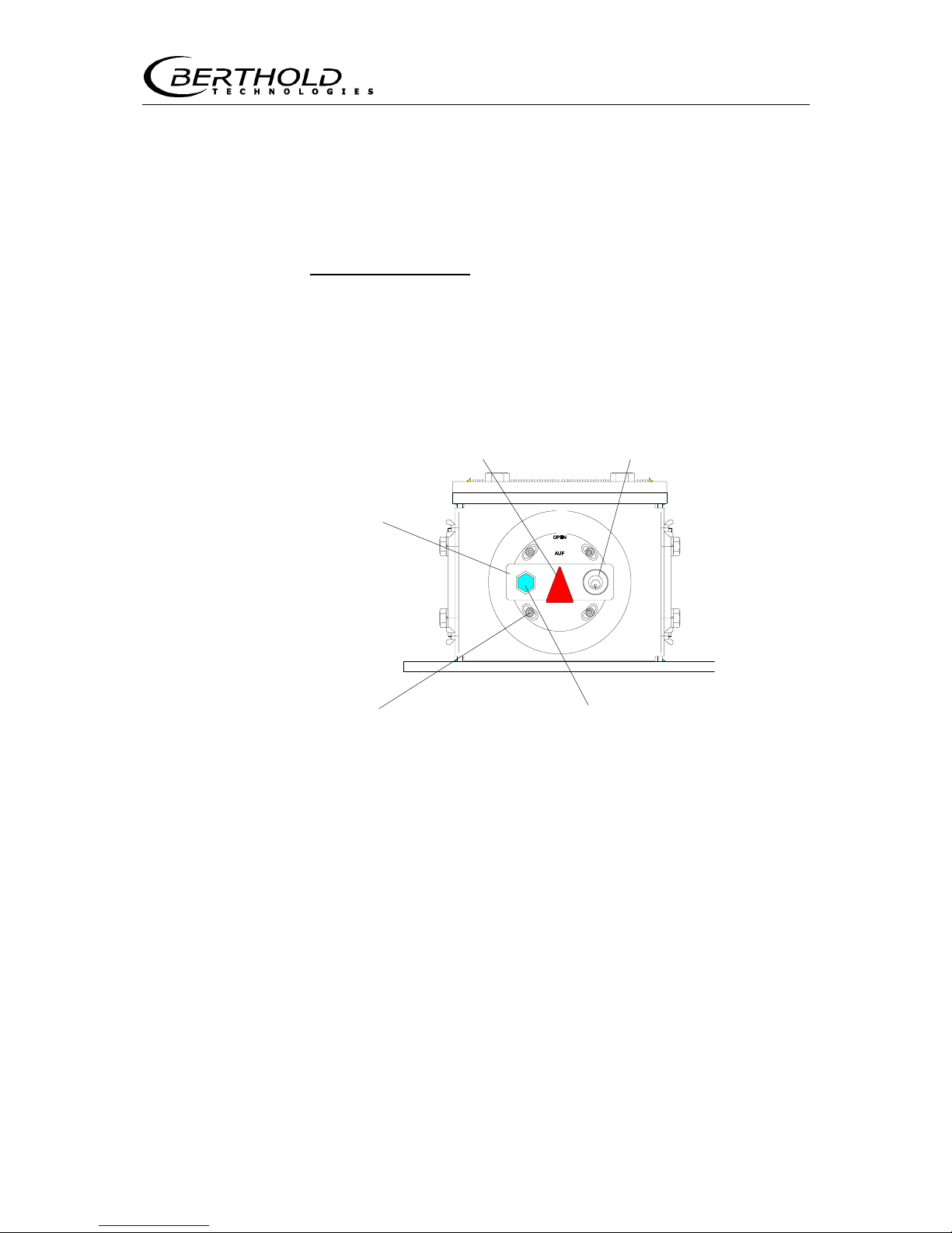
5.2.1 Opening the Radiation Exit Channel
(e)
OPEN position (c) Lock
(d) Threaded (b) Hexagon head cap screw for
bore hole arresting the shielding
Figure 24: Shielding (side view) in foot of measuring frame
Display: radiation exit channel OPEN
Opening the radiation exit channel)
1. Unscrew hexagon head cap screw (b) at lever (a).
2. Insert key in lock (c).
3. Push in lock and turn key to open the lock. Now you can move
the radiation exit channel by turning the lever (a).
4. Turn lever until the arrow points straight up and the bore hole
on the metal plate sits over the respective threaded bore hole.
5. Turn in hexagon head cap screw and tighten it firmly (!). The
source must sit absolutely tight, so that possible vibrations of
the conveyor system cannot move the source in the shielding.
6. Turn key in lock and pull it out.
Lever (a) for
turnin
g
the
shielding
Page 42
5.2 Getting Started
40
5.2.2 Re-adjusting the Detector
Proceed as follows to ensure that the detector is in the optimum
position, i.e. exactly vertical above the source:
❏ Loosen holding of detectors slightly, so you can move it.
❏ Push <run> button of evaluation unit. The measured counts are
displayed.
❏ Carefully move the detector forward and back to find the posi-
tion where it is measuring the most counts.
❏ If you have found the correct position, fix the detector with
screws so it cannot move anymore, not even if vibrations occur.
❏ Push <run> once more to stop the measurement.
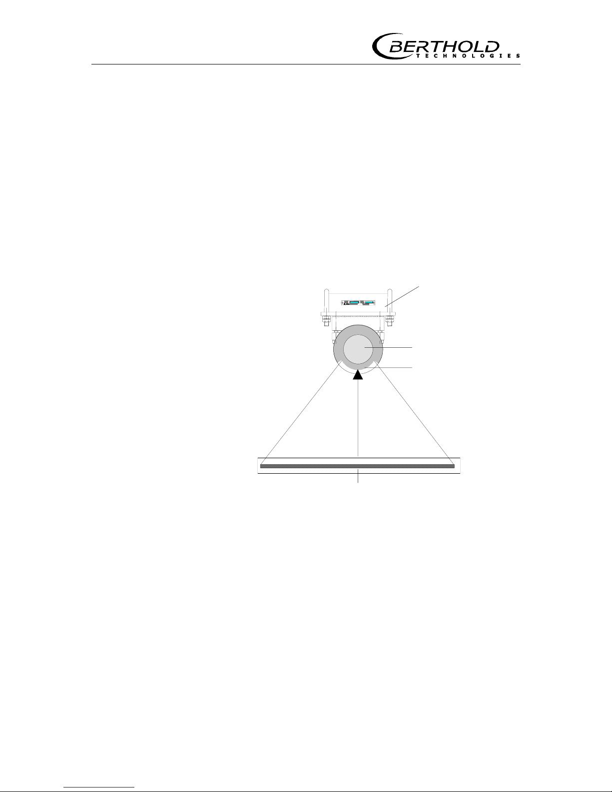
Rod source
Figure 25: Detector window facing the source
Schematic layout
Detector holder
Detector
Detector window
Page 43
Section 5 Getting Started
41
5.2.3 Basic Settings
These steps apply to commissioning as well as to any new
setting of the system.
To enter numbers, select the entry position with <> and the
number you want with <^^^>. Confirm any selection or new entry with <enter>. By pressing <run>, you can go directly to the
Live display (except in the Service menu).
1. Press <more> to select the General Data / Operating Mode
menu group.
1.1 Press <sk1> to select the General D ata menu and then press
<more> to scroll through the parameters:
- Enter password and unlock or lock with <enter>
- Check Date & Time and correct it, if necessary
- Check Instrument Version (e.g. LB 442, Version: 1.10)
- Select Language
- Print Parameter, only if needed
- Factory Setting, only if needed (see also System Configuration,
page 49)
- Return to the menu group with <done>.
1.2 Press <sk2> to select the Operating Mode menu and then
press <more> to scroll through the parameters:
- Select Config Instrument with <^^^> and confirm with <en-
ter>:
- Constant belt speed or
- with moisture compensation or
- with tachometer
- Select Unit: t, kg or kg/m .
- Define Device address: Master or slave instrument
- Specify Detector no.
- Define Error Mode
- Select parameters for RS232 and RS 485 Interface (as needed)
Return to the menu group with <done>.
2. Press <more> to select the Measuring Parameter / I/O C on fig .
menu group.
2.1 Press <sk1> to select the Measuring Parameter menu and
then press <more> to scroll through the parameters:
- Select Measuring Product
- Select Isotope
- Select Measure Mode (e.g. continuous)
- Enter Time Constant (e.g.: 20 s)
- For constant belt speed: define Belt speed
- For moisture compensation: define Current Input, Current in-
put limits and Belt speed
- With tachometer: define Current Input and Current Input
limits
- Enter Belt width
- Select Product select external or internal
Page 44

5.2 Getting Started
42
- Enable/disable Low load suppression. When enabled, enter low
load in tons.
- Select if Mass integrator is to be cleared after each run (=yes
or if the count should continue (=no).
Return to the menu group with <done>.
2.2 Press <sk2> to select the I/O Config menu and then press
<more> to scroll through the parameters:
- Select Product
- Select Current output 0 or 4 (26a/26c)
- Define Current output limits 0/4 and 20 mA for load
- Define Current Output Error: Hold last measured value or enter
mA value
- Define digital input 1: Belt stop or Erase mass integrator or
batch mode
- Define digital input 2: External tare or Print start, Product 3+4
or Start / Stop and print
- Define Relay 3: Tare measurement or Batch Ready or
Min/Max.
- For Batch Ready enter desired batch weight.
- For Min/Max enter threshold value and hysteresis.
- For Mass counter select tons per pulse
- Data printout: Select none or Minute prints or Shifts. For shift
printout, enter the respective parameters.
- Return to the menu group with <done>.
Page 45

Section 5 Getting Started
43
5.2.4 Calibration
Calibration is carried out in 2 steps.
a) the tare measurement and
b) the actual calibration
a) Tare Measurement
Before starting up the measuring system, the zero or tare weight
has to be determined.
The tare weight changes constantly as a result of conveyor irregularities, such as variation of the thickness of belt or, as in the case
of chain conveyors, differences between chains links and scrapers.
During tare determination, therefore, the conveyor must run and
the average value must be determined over a few complete conveyor belt cycles. The rule is: the more cycles, the more precise
the result.
Proceed as follows:
□ Select Calibrate menu and the submenu sk1: Tare Meas.
□ Select operating mode for tare measurement: Time or
Length.
□ Time: enter measuring time in seconds and confirm with
<enter> (see also section 7.1).
□ Length: enter the belt length in meters and confirm with
<enter> (see also section 7.1).
□ Empty conveyor system and make sure that it remains
empty over the entire measuring time.
□ Push the <run> button. The tare measurement starts
and the tare count rate is displayed.
□ At the end of the measurement, the averaged tare count
rate and the selected belt length or time is displayed.
□ Store the measured value with <enter>.
For more information see Tare Measurement page 68.
Page 46

5.2 Getting Started
44
b) Calibration
Proceed as follows
□ In the main menu, select sk1: Calibrate and then the
sk2: Calibrate
submenu.
□ Select the product to calibrate (no. 1...10). Select the
same product number in the Me asuring Parameter
menu!
□ Select sk1: Data Input submenu.
□ Load product on conveyor belt and start conveyor belt.
□ When the product has reached the measuring frame,
push the <run> button. The computer starts counting
the time and averages the count rate and speed over the
measurement.
□ If the material used for comparative weighing has
passed the measuring frame, push <run> to stop the
measurement. The averaged count rate and belt speed
as well as the measuring time is displayed.
□ If you confirm the 3 values with <enter>, the prompt
Comparative weight appears.
□ Enter result of comparative measurement.
□ Confirm value with <enter>.
□ Go to next calibration point with <more>. To use an-
other calibration point, proceed as described. To use no
further calibration point, enter „0“ cps at the following
Rate and confirm with <enter>. The values of this and
all following calibration points are then not
used for cal-
culation of the calibration curve.
□ Press <more> to scroll through the calibration points
that are not used. The display returns to the submenu
group sk1: Data Input/sk2: Calculate
.
□ Select sk2: Calculate.
□ Select calibration mode lin/squ/cub/auto. Calibration is
performed as soon as you confirm the calibration mode
with <enter>.
□ Then you can call the results with <more>: depending
on the selected calibration mode: linear/square/cubic
coefficient; and square error.
□ If necessary, enter a Factor or an Offset (see section 8.2
"Correction of Display Value " on page 77).
Page 47
Section 6 Evaluation Unit LB 442
45
Section 6 Evaluation Unit LB 442
6.1 General Description
The evaluation electronics is designed as a 19" module in the format 3 HE, 21 TE. It includes the microprocessor-controlled evaluation electronics and the power supply for the operating and control
voltages. A 32 bit microprocessor with a menu-structured software
specially designed for bulk flow measurements is used for signal
processing.
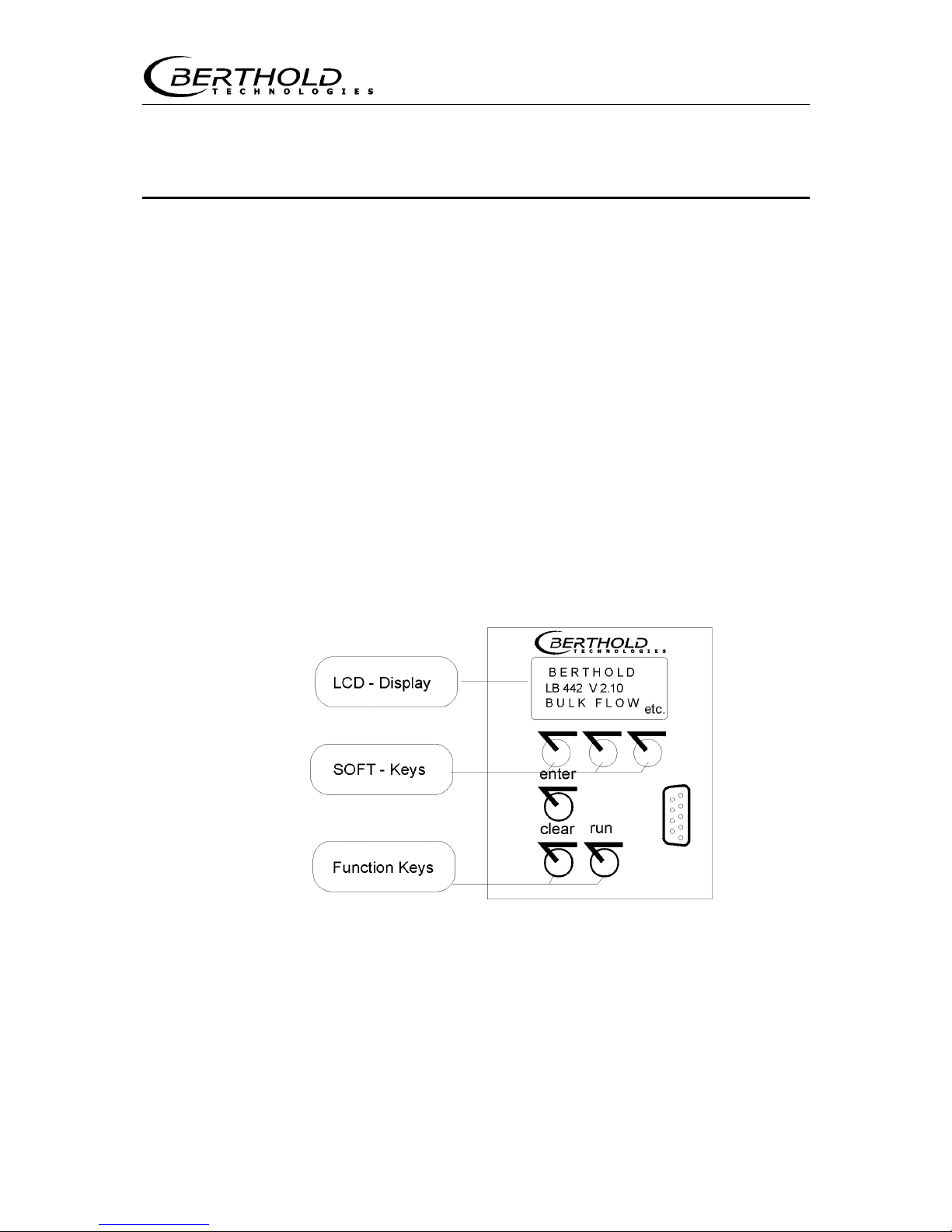
Six foil keys on the front panel are all you need to operate the instrument:
o Three so-called softkeys allow user-guided definition
of all instrument settings and input of the required
parameters.
o Three more function keys: <enter>, <clear> and
<run>.
The illuminated display field on the front panel shows the relevant
instrument function on four lines. The front panel also includes a
RS 232 interface.
Figure 26: Front Panel LB 442
The terminal strip on the instrument rear panel includes all terminals for power supply, for the detector, and for the analog and
digital output signals. The current output is isolated and the builtin relays for Max./Min. signaling and for error messages include an
isolated contact.
The system automatically corrects for the decrease of the source
activity over the entire service life of the source.
System malfunctions are signaled by error messages.
Page 48

6.1 General Description
46
The calibration data is stored in a FLASH memory and saved in
case of power down.
The operational safety of the evaluation unit and the detector is
ensured by a permanent self monitoring with error code display
and by plausibility checks; all important data are saved in a Flash
memory.
Display
The illuminated display field of the instrument comprises 4 lines;
the first three lines show the menu titles, the currently selected
parameters or the current measurement value. The bottom line
shows the current function of the softkey button located below or,
when a measurement is running, the status “run“.
Keypad Function
The evaluation unit is operated via the softkeys and function keys
described below; with these keys you can select the operating level
you want within a menu structure in order to select a function or
enter parameters. The menu guidance is illustrated in the quick
overview of the menu structure (see next page) and from the tables giving an overall view of the menu structure (see the Appendix).
Softkeys
Softkeys are used to select different menu groups and operating
levels within the menu structure. Depending on the current position in the menu structure, functions are assigned to these keys,
as shown on the display above the respective key.
Page 49
Section 6 Evaluation Unit LB 442
47
Softkeys
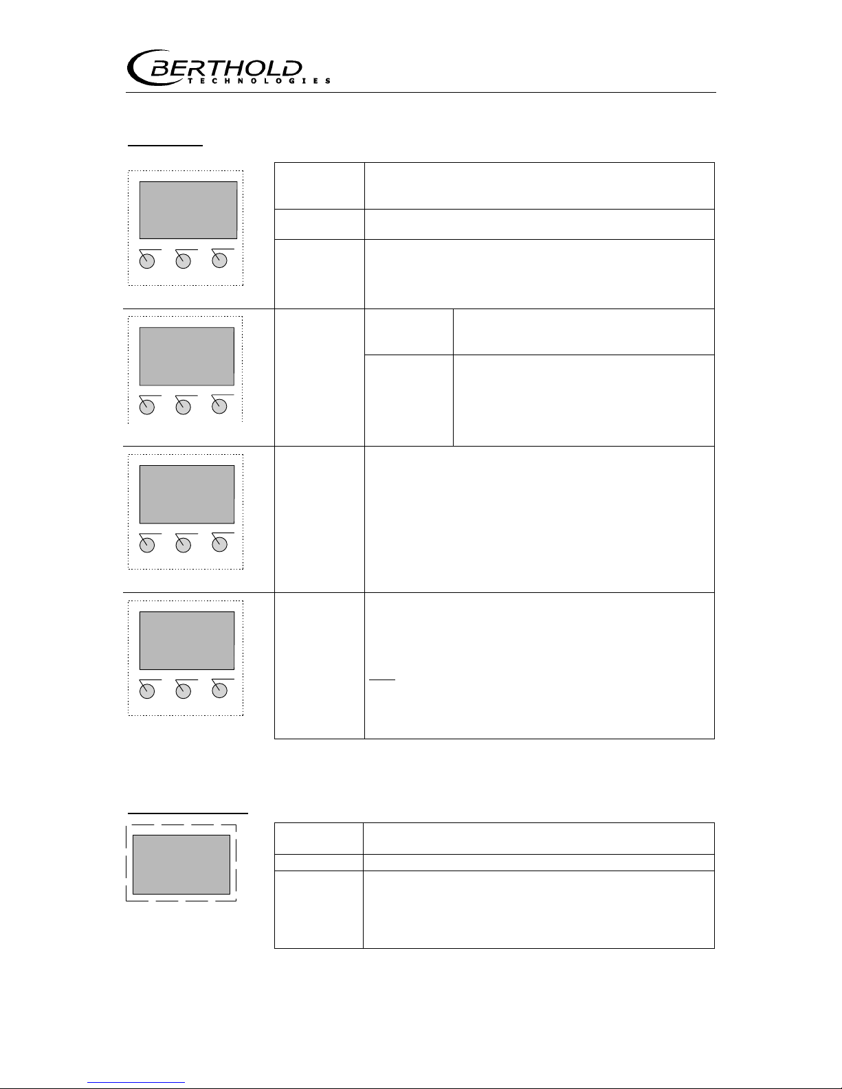
Figure 27: Softkey functions
Function keys
<enter>
accepts the entry and moves the cursor to the next
input field or toggles between two input fields..
<clear> clears the numerical value.
Load
2300 t/h
+ - RUN more
Figure 28:
Live display
<run>
starts or ends a measurement or leads directly back
to the display and at the start of a measurement
automatically changes to the live display
<sk1
>
<sk2>
Invokes the indicated menu
(Figure 27a)
<more> Invokes the next display or menu group.
sk1: General Data
sk2: Operating Mode
sk1 sk2 more
<done>
Shows the end of the menu and takes you back to
the menu group.
Text:
scrolls through the various select options
Product select
[external/internal]
^^^ done
internal
<^^^>
Numerical
values:
increments the number marked by the
cursor by 1.
Time Constant
more
value: 20.000
←←←←←←←←←←←←
∧∧∧
∧∧∧∧∧∧
∧∧∧
<
>
moves the cursor to the left and at the end of the
input field again to the start position
HV (500): 112 cps
+ - exit
HV (560): 116 cps
HV (620): 122 cps
<+>
<
->
scrolls cyclically in a result list or in the
Live
display
Page 50
6.1 General Description
48
6.1.1 Menu Structure (Flow Chart)
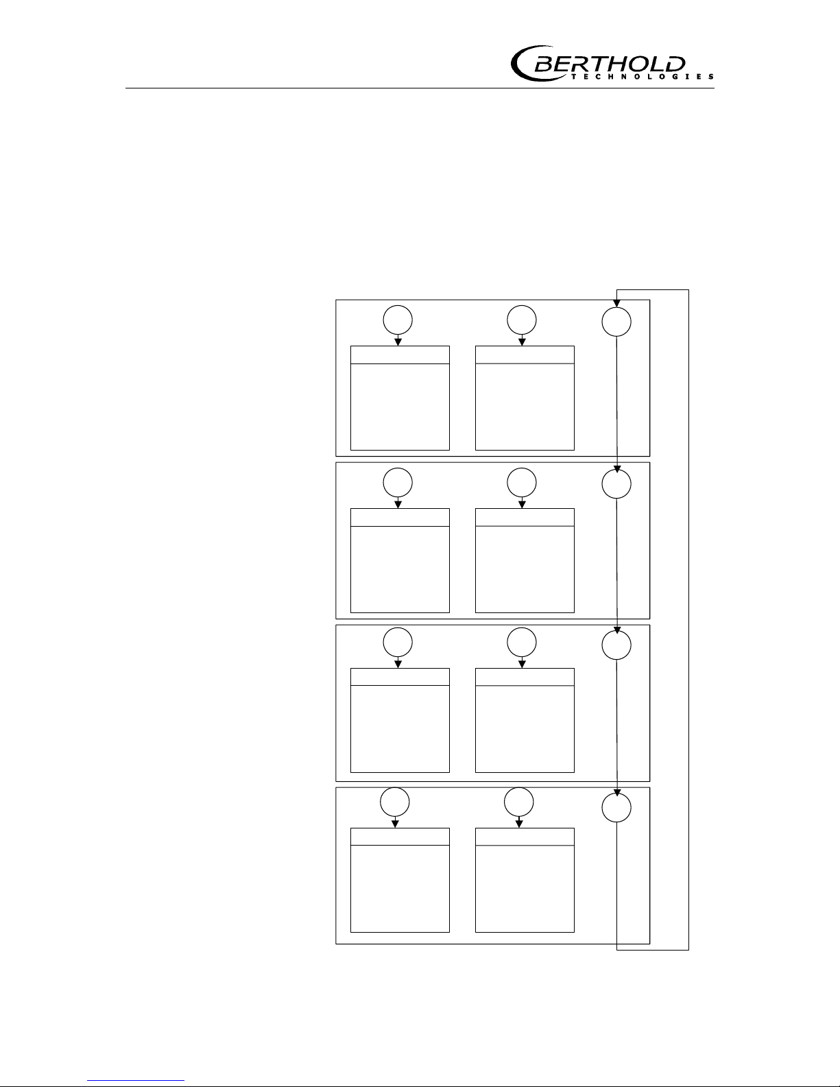
The flow chart below illustrates the menu structure for parameter
input and operation. With <more> you select the various menu
groups and from there you get to the respective menu with <sk1>
or <sk2>. Within the menu you get to the individual windows with
<more> and at the end of the menu you get back to the menu
group with <done>.
General Data
Password
Date & Time
System Version
Detector Soft.
Language
Parameter Print
Factory Setting
Operating Mode
Config. Instrument
Tacho Config
Unit Selection
Error Mode
Loading at Stop
sk1 sk2
Measure. Parameter
Detector / Isotop
Time Constant
Belt Speed
Basis Weight
Width of Belt .
Product Selection
Erase Massintegr.
I/O Config.
Product Selection
Current Output
Dig. In 1 / 2
Dig Out 3
Print Out
sk1 sk2
Calibrate
Tare
Data Input
Calibration Mode
Factor Offset
Live Display
Loading
Totalizer
Detector Temp.
Tare Counts
Speed
Detector HV
Count Rate
sk1 sk2
Service Menu
Test
I/O Test
HV Set-Up
Status Request
Plateau
Current Out Adjust
Pulse Length
Interfaces
RS 232/485
Access Control
Number of Detectors
Slave Address
sk1 sk2
more
more
more
more
Figure 29: Menu structure
Page 51
Section 6 Evaluation Unit LB 442
49
6.2 Software Functions and System Configuration
The factory settings are listed in the Configuration Checklist in the
Appendix. Enter the final operating settings in this list. Please keep
in mind that the entry in all operating levels is made with the
<^^^> key and the new value is accepted with <enter>.
The menu structure on pages 147 to 150 provide a general functions overview.
General Data
Password:
You can enter a number comprising up to 6 digits. Upon confirmation with <enter>, the system is protected against unauthorized
manipulation of the parameters. All parameters can still be viewed,
however. Password protection is canceled when you enter the correct numerical value and confirm your entry with <enter>.
Date:
Enter the current date in the format TT.MM.YY. The correct date is
important for automatic correction of the activity decay of the rod
source.
Decay compensation is performed every night at midnight or when
pressing the <run> button to start the measurement modes, when
the last decay compensation took place more than 24 hours ago.
The tare count rate and the count rates of the individual calibration
points are corrected.
Time:
Enter the current time in the format HH.MM.
System/Version:
Display of instrument type and software version.
Detector software version:
Display of the software version of the connected detector.
Language:
You can choose German, English or French as dialog language by
pressing the <^^^> key.
Page 52
6.2 Software Functions and System Configuration
50
Print Parameter:
A printer with serial interface can be connected via the 9-pole connector on the front panel. Use a commercial zero modem cable to
connect the evaluation unit with the printer. (In a zero modem ca-
ble outgoing and incoming lines are crossed.)
Push the <enter> button to print all parameters for documentation. The printout in the appendix shows an example. A PC may
also be connected and the data transferred to the computer and
processed there using a terminal program.
See Example printout on page 128.
Factory Setting:
All parameters can be reset to the factory setting by pressing
<sk1> and <clear> at the same time.
The current calibration data is lost when the instrument is
reset!
Operating Mode
Config Instrument ::
The instrument configuration is defined by the required measuring
configuration and the measuring task and can be selected by
pressing <^^^> and <enter>.
o Const. belt speed
Measurement with constant belt speed. The speed is entered as a
fixed value.
o with moisture compensation
Measurement with moisture compensation by feeding the moisture
signal 0/4 – 20 mA (terminals 28a and 28c).
o with tachometer
Measurement with tachometer (terminals 28a and 28c). Depending
on the tachometer used, choose either:
Tacho input
(only if operating mode with tachometer has been selected)
Tacho input as pulse input
Tacho input as current input
Tacho pulses/revolution
(only if Tacho input as pulse input has been selected)
Choose between tachometer types for 500, 2500 or 5000 pulses
per revolution
Tacho drive
(only if Tacho input as pulse input has been selected)
Page 53

Section 6 Evaluation Unit LB 442
51
o Running wheel:
The running wheel is placed onto the conveyor belt.
o Drive shaft:
The tachometer is connected with a shaft via a coupling.
Forward feed per revolution
(only when tacho drive with motor shaft has been selected)
Forward feed = distance of conveyor belt at one tachometer revolution.
Input in mm.
Select unit [t]/[kg]/[kg/m]
Select the unit.
o [t]/[kg]
If t or kg is selected, the measurement is carried out in t/h or
kg/h. For calibration, you have to enter a comparative weight in t
or kg.
o [kg/m]
If kg/m is selected, the measurement is carried out in t/h.
For calibration, however, you have to determined a comparative
weight in kg/m.
See also "Calibration in kg/m" and "Static Calibration" on page 72.
Error mode
Select if the measurement is to be aborted or continued if an error
occurs. If you select „continue“, the error message is only displayed, but the system continues measuring. Push <enter> to
clear the error display.
Curr. outp error:
o Hold
If any error is detected and the measurement is interrupted because of the error, the current output holds the last current value.
o Value
If any error is detected and the measurement is interrupted because of the error, the current output switches over to a predefined
current value.
Load in case of stop
o Hold
If the measurement is stopped externally or via the "run" button,
the display and the current output will hold the last value.
o Value
If the measurement is stopped externally or via the "run" button,
the conveying capacity on the display switches over to 0 t/h and
the current output to 0 or 4mA.
Page 54
6.2 Software Functions and System Configuration
52
Measuring Parameter
Detector and Isotope
o Detector code:
Detector-specific code number for automatic high voltage control.
Detector list
Scintillator Type Dimensions
mm
Weight
kg
Detector
code
NaI Plastic
LB 4401-01
LB 5401-01
25/25 6 0
X
LB 4401-02
LB 5401-02
40/35 6 0 X
LB 4401-03
LB 5401-03
50/50 18 0 X
LB 4405-01 500 10 22 (24) X
LB 4405-02 750 10.5 22 (24) X
LB 4405-03 1000 13 13 (15) X
LB 4405-04 1250 13.5 13 (15) X
LB 4405-05 1500 15 10 (12) X
LB 4405-06 2000 22 10 (12) X
Detector code in () can be used to reduce the background. Any
change in the detector code requires a new calibration.
o Isotope Select:
Select the isotope used for the measuring configuration so that the
nuclide-specific factor for the automatic half-life correction becomes effective for automatic decay compensation. You can select
either Am/Co/Cs/Kr/Cm.
Page 55

Section 6 Evaluation Unit LB 442
53
Time Constant 1 1 (0 to 9999,9 sec):
Enter the time constant in seconds. The computer calculates a sliding average of the area weight over this time. The higher the time
constant entered, the lower the statistical variations of the output
signal, the longer, however, the response to sudden changes
- Time constant 2
(Only available via the button combination SK1 & clear.)
This time constant smoothes the statistics of the count rate prior to
the calculation and is independent of time constant 1. In most
cases, the standard value of 1 s is correct. Any change of this time
constant should be made only after consultation with BERTHOLD
TECHNOLOGIES.
- Time constant for tacho or moisture input
(Available via Time constant 2 + <more>.)
This time constant smoothes the current input. In most cases, the
standard value of 1 s is correct. A higher value will smooth the
measured value at the current input more, but at the same time
delays the response to the load.
Curr. Input
(Only when operating mode with moisture compensation has
been selected)
Select the initial value 0 or 4 mA of the current input signal
(28a/28c).
Curr. Input limits
(Only when operating mode with moisture compensation has
been selected)
0/4mA lower limit value in % moisture
20 mA upper limit value in % moisture
or
(Only when operating mode with tachometer with current in-
put has been selected)
0/4mA lower limit value in m/s
20 mA upper limit value in m/s
Belt speed (0 to 99,99 m/s)
(Only when operating mode constant belt speed
or with moisture compensation has been selected)
Enter the constant belt speed in m/s.
Page 56

6.2 Software Functions and System Configuration
54
Max. Basis Weight
For non-linear calibration curves you have to enter the maximum
weight per area and you have to select the function cubic for calculation. These square or cubic characteristic curves require absorption coefficients a2 and a3 in addition to the absorption coefficients
a1. This kind of calibration curve is required only in rare cases. In
such cases you then have to enter the maximum weight per area
at maximum load in g/cm
2
prior to calculation. Without this information, you will get the following error message when you try to
perform a cubic calculation: "Enter weight per area".
The weight per area is calculated as follows:
M (t/h)
F (g/cm
2
) = -------------------------------
v (m/s) x b (m) x 36
Example:
Measuring range: 0 – 200 t/h
Belt speed v: 1 m/s
Belt width b: 1 m
F = 5,55 g/cm²
Belt width (0 to 9,99 m)
Enter the belt width in meters for calculation of the weight per area.
Product select [external/internal
Specify if the product is to be selected via the evaluation unit (=
internal) or via digital inputs (= external, 18a and 18c, 20a and
20c).
Low load suppression
The low load entered here is suppressed and as long as the entered value in t/h (kg/h) is not exceeded, the display shows 0 t/h
(kg/h).
Erase mass integ.
Yes means: reset the mass integrator to zero for each new run.
No means: The mass integrator continues to count from the value
reached last in each run.
Page 57

Section 6 Evaluation Unit LB 442
55
I/O Config.
Define the inputs and outputs separately for each product. These
parameter settings are valid for calibration and measurement.
Product Select
No. 1 ... 10
Select the product number for which this parameter setting is to be
valid.
Current output :
Select the start value 0 or 4 mA of the current output signals
(26a/26c).
Curr. Outp limits (26a/26c):
0/4 mA: lower limit value in t/h (kg/h)
20 mA: Upper limit value in t/h (kg/h)
Curr. Outp Error:
Fault current: HOLD or VALUE:
You can select if the last measured value should be held in case an
error is detected ("HOLD"), or if an arbitrarily selected value between 0 and 22 mA should be set. The requested value has to be
entered after selecting "VALUE".
Digital Input
o Digital Input 1
Define the configuration of digital input 1 (terminal 18a and 18c).
Up to three different functions can be assigned to the input.
- Belt stop
With closed contact the measurement is stopped and the last
measured values is held. This function can be used only at constant belt speed.
- Erase mass integrator
If the input is short-circuited, the mass integrator is reset to 0 t.
- Batch mode
Start of an external batch measurement. Relay 3 must also be set
as Batch Ready.
Start
The measurement starts when the contact is closed. The mass
counter starts at 0 t. Contact of relay 3 is open.
Stop
The measurement stops as soon as the specified batch weight is
reached. Contact of relay 3 is closed. The batch weight obtained is
held until the next start.
Page 58
6.2 Software Functions and System Configuration
56
o Digital input 2
Define the configuration of digital input 2 (terminal 20a and 20c).
Up to three different functions can be assigned to the input.
- External tare
An external tare measurement is performed. The elapsed tare time
is dependent on the tare measuring time entered.
- Print start
When the contacts are closed, the measured values are printed
out.
- Ext. product 3+4
Digital input 2 can also be used to expand the external product selection. In this case, the different products can be selected as
shown in the table below:
Menu Dig. input 2 Dig. input 3
1 0 0
2 0 1
3 1 0
4 1 1
1 = closed contact
0 = open contact
Table for external product selection 3+4
- Start/Stop and print
If the contact closed, a tare measurement is carried out first. Then
the measurement automatically changes over to the measurement
mode. The measurement mode is interrupted as soon as the contact is opened. After the measurement, a printout is created automatically, including date, time and measured tonnage.
Digital output relay 3
Define the configuration of digital output 3 (terminal 14a and 14c).
Up to three different functions can be assigned to the input.
- Batch Ready
(Only with setting Batch mode at digital input 1)
When the defaulted tonnage is reached, a relay signal is output at
relay 3.
- Min / Max
Signals exceeding or falling below a load limit value. Enter the
lower or upper threshold in t/h or kg/h. An open contact signals
that the threshold is exceeded or not reached.
- Tare measurement
Signals the end of a tare measurement. The contact is closed during tare measurement.
Page 59
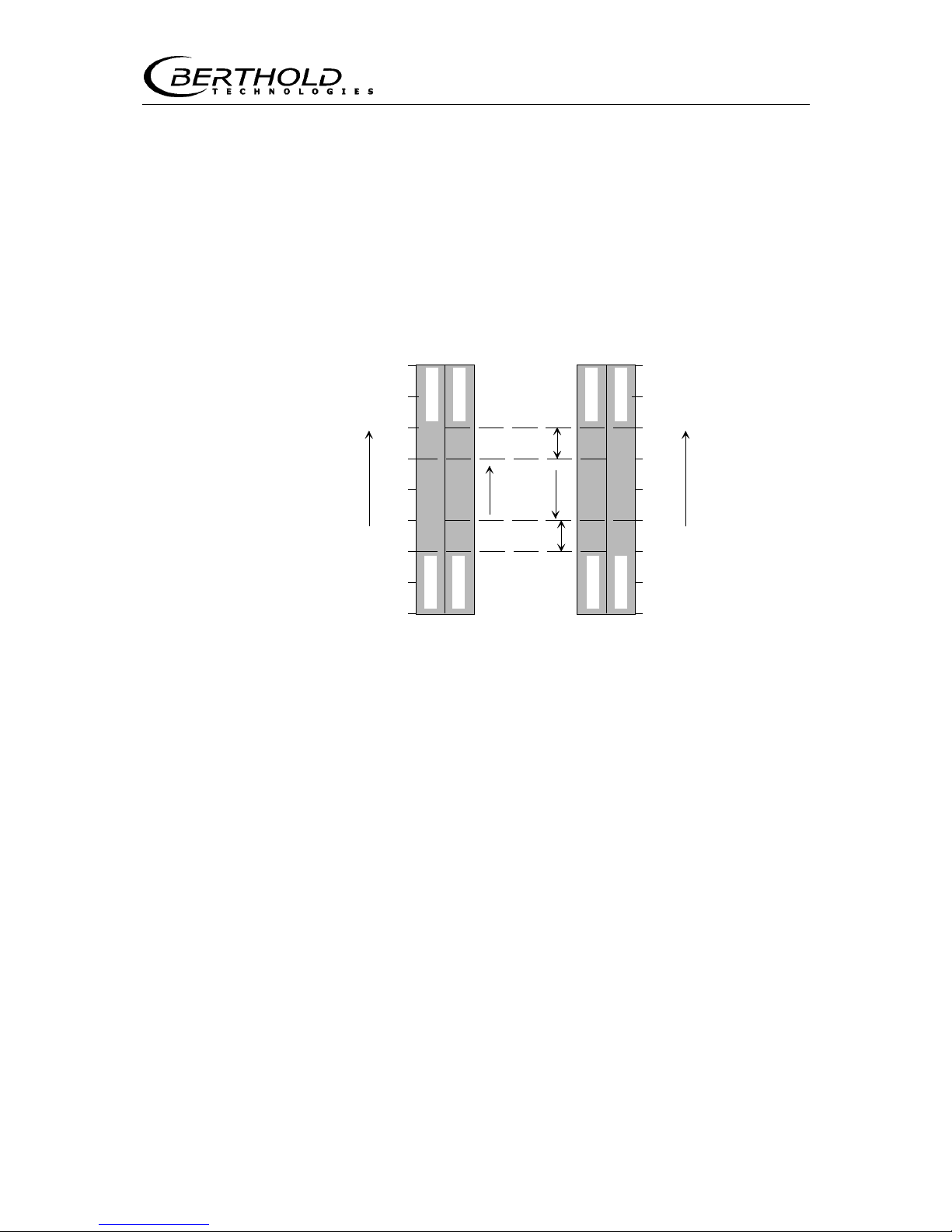
Section 6 Evaluation Unit LB 442
57
Hysteresis
(Only with setting Min / Max at digital output 3)
Enter the hysteresis in the selected unit. A switch-over of the relay
is triggered only when the change of the measured value is greater
than the entered value. Depending on the setting as Max. or Min.
function, the relay is de-energized (circuit opening connection)
when the selected value is exceeded or not reached. If the displayed value drops again, the relay picks up again, delayed by the
value of the selected hysteresis. The switching hysteresis should
be about 5%.
Rel.
min.
1.0
1.2
1.4
1.6
1.8
Rel.
min.
Rel.
max.
Rel.
max.
3
Densityin g/cm
Hysteresis
1.0
1.2
1.4
1.6
1.8
Signal
rising
Signal
falling
Hysteresis
de-energized
energized
de-energized
energized
energized
de-energized
de-energized
energized
3
Density in g/cm
Figure 30: Diagram illustrating the hysteresis
Batch weight
(Only with setting of Batch mode at digital input 1 and Batch
Ready at digital output 3)
Value:
Enter the batch weight in the selected unit (t or kg). During batch
measurement you will get a signal when the batch weight entered
here is reached. The measurement stops.
Ext. mass counter:
o Tons per pulse
A pulse is output as soon as the tonnage defined has been
reached. The following tonnage values can be set:
Off - 0.01t - 0.1t – 1t – 10t
Example:
With setting 1 t, a pulse is output after each integrated tonnage.
The pulse length can be changed in the Service menu and is set to
50 ms as standard value. If Off is selected, no pulse is output.
Printout Data on Printer
o No
No result printout.
o Minute prints (1 to 999 min)
Enter an interval in minutes for the printout.
Page 60

6.2 Software Functions and System Configuration
58
o Shifts
Define the shift parameters:
- Begin Shift
Enter the time (hh:mm)
- Shifts/Day
Number of shifts per day
- Hours/Shift
Number of hours per shift.
Tare measurement
Tare measurement at
Time or belt length default
Select the measurement mode for the tare measurement:
Time
(Only when Time has been selected)
Enter the measurement time in seconds.
Length
(Only when Length has been selected)
Enter the belt length in meters over which tare has to be measured. This value should include even-numbered belt cycles.
Example:
If the belt length for one cycle is 51 m and you want to measure 5
belt cycles, you have to enter the value 255 m.
Rate:
Read in
the tare count rate by pressing <run>. When Time is se-
lected, the remaining measuring time is displayed in addition; with
Length the remaining belt length.
Press the <enter> button at the end of the measuring time or belt
length to store
the tare count rate and the calibration data (not
displayed).
Interrupting the tare measurement:
The tare measurement can be interrupted any time and started
again by pressing <run>. The previously measured average value
is not lost during this interruption; averaging continues after restart of the measurement. For more information see section 7.2
Tare Measurement.
External tare measurement
is started by short-circuiting terminals
20a and 20c, carried out fully automatically and the result stored
with date.
During tare measurement the current output
(26a/26c) does not
supply any current.
The tare count rate can also be entered manually
.
Calibrate
Page 61
Section 6 Evaluation Unit LB 442
59
Product Select
No. 1 to 10
Select the calibration product and confirm with <enter>. Please
note that the product number set in the Measuring Parameter
menu is identical with the product number selected here. Otherwise, no calibration measurement is possible, but only manual entry of the calibration data sets since the <run> button is locked.
Data Input
Background for rod detector
If a rod detector is used, you have to enter the background. The
count rate is read in over a period of approx. 60 s. The measurement is started and stopped by pushing the <run> button. The
value confirmed with <enter> is saved.
For more information on this subject please see Background on
page 68.
1. Value to 10. Value
For calibration of the radiometric bulk flow measurement you can
enter or read in max. 10 calibration points. You need at least 1
calibration point, but you have to run through all 10 points.
Calibration points with zero values are not calculated. If a calibration point includes a count rate with „0“ cps, this and all following
calibration points are not used for calculation.
Values confirmed with <enter> are stored, so that the individual
parameters and measured values are always available. Therefore,
the calibration points can be entered at different times.
With the <enter> button you can scroll through the individual
units of measure for the respective calibration points. The cursor
position indicates the active row.
Press the <more> button to display the next calibration point.
Tip: Write down all values of the calibratio n po ints immediately.
In this manner, you can easily correct incorrect entries in the calibration points.
Before recording a calibration point, you should determine
and enter the tare count rate. In the other case, also when
the tare count rate is entered later, the count rates in the
calibration points change.
See also chapter 7.2.2 Tare Compensation on page 70.
Page 62
6.2 Software Functions and System Configuration
60
Display per calibration point
- Rate (cps)
Read in the calibration count rate by pressing <run>.
Stop the calibration measurement by pressing <run> again.
Press <enter> to accept the values.
The calibration count rate can also be entered manually.
- Speed (m/s)
Automatic display of the averaged belt speed.
- Measuring time (s)
Display of measuring time.
- Comparative weight (t)
Enter the comparative weight for this calibration point. This value
can be entered before or after the calibration measurement.
Note: After the calibration measurement has been stopped,
confirm the respective measured value with <enter>; otherwise it will be rejected when you quit the respective calibration point.
See detailed discussion in section 5.2.4 b) Calibration on page 44.
Page 63
Section 6 Evaluation Unit LB 442
61
Calculate
Calibr. Mode
Select the calibration mode.
lin/squ/cub/auto
- lin
Linear curve fit
. This mode is used when at least one calibration
point is available in addition to the tare measurement. Linear calibration is the most frequently used type of calibration. For more
information see chapter 5.2.4 b) Calibration.
Square curve fit
cannot be selected. Please use the cubic calibra-
tion function instead.
- cub
A curve fit using cubic coefficients
should be applied when at least
3 value pairs are available and a linear curve is not sufficient. In
this case you have to enter the maximum weight per area as well.
See also on page 54.
- auto
The program automatically selects the best curve fit
. Square or
cubic curve fit are used only when it can be ruled out with 95%
probability that the values correspond to the curve only by chance
(check by means of f-test).
If more than three calibration points are used for a calibration of the curve, then we recommend to plot the calibration
points. In this x/y plot, the load (t/h) should be a function
of the count rate LN (cps).
LN (cps) = natural logarithm of the count rate.
Upon selection of the required calibration mode and pressing of the <enter> button, the calibration factors are calculated.
Page 64

6.2 Software Functions and System Configuration
62
Coeff. a1
Linear absorption coefficient.
This value is calculated automatically during linear calibration.
Coeff. a2
Square absorption coefficient. This value is calculated automatically for a cubic multi-point calibration.
Coeff. a3
Cubic absorption coefficient. This value is calculated automatically
for a cubic multi-point calibration
Square Error
This value is calculated automatically for two- and multipoint calibration. It provides information on the quality of the calibration
curve. The smaller the numerical value, the better the curve fit
(see section 7.2). This coefficient is not a criterion for selection of
the best calibration mode (see calibration mode auto).
Factor
Option: You can enter a multiplicative factor to correct the load.
The load is multiplied with this value. When running another calibration, this value is automatically set to "1" (see also section
Factor).
Offset
Option: The offset (-9999.99 to +9999.99) for additive correction
of the load. The value entered here is added to the load. When
running another calibration, this value is automatically set to "0"
(see also section Correction of Display Value on page 77).
If you notice a constant positive or negative deviation over the entire measuring range, i.e. for high and low loads as well as with
empty belt, a new tare measurement has to be performed. If this
is not possible the error can be corrected by entering a positive or
negative numerical value in t/h.
Page 65

Section 6 Evaluation Unit LB 442
63
Live Display
In this menu, the measured values are displayed continuously (live
display) for the selected product (display of RUN); otherwise the
values of the last measurement.
With <+> and <-> you can cycle through the following displays.
Start measurement
A measurement can be started from any menu item by pressing
the <run> button (exception: Service menu and calibration
points). Then the load is displayed. RUN appears on the display.
With <more> you can invoke further live displays and you can
scroll through them with <+> and <->. If the measurement is
stopped by pushing the <run> button, the load on the display and
at the current output switches to 0 t/h (kg/h) or shows the last
measured value. See also function "Load in case of stop" on page
51.
Totalizer (t or kg)
Display of integrated total weight in the selected unit.
If you continue with <->, the following menus appear:
Load (t/h or kg/h)
Display of load in the selected unit
Load dry (t/h or kg/h)
Display of dry load in the selected unit (only in operating mode
with moisture compensation).
Load total (t/h or kg/h)
Display of total load in the selected unit.
Detector temp. °C
Display of detector temperature
Tare Cps [Cps]
Display of tare count rate.
Act. count rate [Cps]
Display of actual count rate with on-going measurement or measured value of last measurement.
Current output actual mA
Display of current output in mA.
Actual belt speed m/s
Display of belt speed
Page 66
6.2 Software Functions and System Configuration
64
Moisture %
Moisture reading when the radiometric bulk flow measurement is
configured accordingly and a moisture meter is connected (only in
operating mode with moisture compensation).
Dry totalizer (t or kg)
Display of dry weight in the selected unit (only in operating mode
with moisture compensation).
Raw data
By pushing the <more> button, the raw data of the connected detectors can be displayed live. The following raw data can be read
for each detector:
HV
Shows the actual high voltage value at the detector.
HV-auto: Automatic HV control is enabled. This is the normal mode
for the HV.
HV test: A manual fixed value has been set in the Service menu.
This setting should only be used for a test.
cps
Display of the unaveraged live count rates of this detector.
Det. Temp.
Display of the detector temperature.
Service Menu
See Service Functions on page 95.
Page 67

Section 6 Evaluation Unit LB 442
65
Interfaces
RS 232.
A commercial zero modem cable is used to transfer data via the
RS 232. The following data can be transmitted via this interface:
- Parameter List
Via command parameter printout in the General Data menu.
- Minute prints
- Shifts
- Batch printout
Via digital 2, provided it has been set to Start/Stop + Print.
Data can be output, depending on the setting, via the following
devices:
o PC
Data output to PC.
o Printer
Data output to printer.
RS 485
The RS 485 can output the same data as the RS 323. In addition,
further detector systems can be connected via this interface.
o PC
Only for data output to PC.
o Printer
Only for data output to printer.
o Slave
Only for further detector systems.
One slave evaluation unit is needed, feeding the additional detector. The count rates from the slave and possible error messages
are send to the master via the RS 485. The further processing is
carried out by the master.
Number of detectors
Enter the number of all detectors in this measuring system.
Slave 1
(Only if Number of detectors
> 1)
Address for slave 1. We recommend to keep standard address 1.
Further addresses have to be used only when more than 1 slave is
connected. Accordingly, you have to enter the same address in the
slave evaluation unit.
Page 68

6.2 Software Functions and System Configuration
66
6.2.1 Slave Menu Functions
General Data
Password:
You can enter a number comprising up to 6 digits. Upon confirmation with <enter>, the system is protected against unauthorized
manipulation of the parameters. All parameters can still be viewed,
however. With password protection enabled, the <run> button is
locked. External measurements such as batch and tare measurements can be started via the digital inputs. Password protection is
canceled when you enter the correct numerical value and confirm
your entry with <enter>.
Date:
Enter the current date in the format TT.MM.YY. The correct date is
important for automatic correction of the activity decay of the
source.
Decay compensation is performed every night at midnight or when
pressing the <run> button to start the measurement modes, when
the last decay compensation took place more than 24 hours ago.
The tare count rate and the count rates of the individual calibration
points are corrected.
Time:
Enter the current time in the format HH.MM.
System/Version:
Display of instrument type and software version.
Detector software version:
Display of the software version of the connected detector.
Language:
You can choose German, French, Spanish and English as dialog
language by pressing the <^^^> key
Print Parameter:
A printer with serial interface can be connected on the front panel
to document all parameter settings. The printout in the appendix
shows an example. A PC may also be connected and the data
transferred to the computer and processed there using a terminal
program.
See Example printout on page 128.
Factory Setting:
All parameters can be reset to the factory setting by pressing
<sk1> and <clear> at the same time.
Page 69
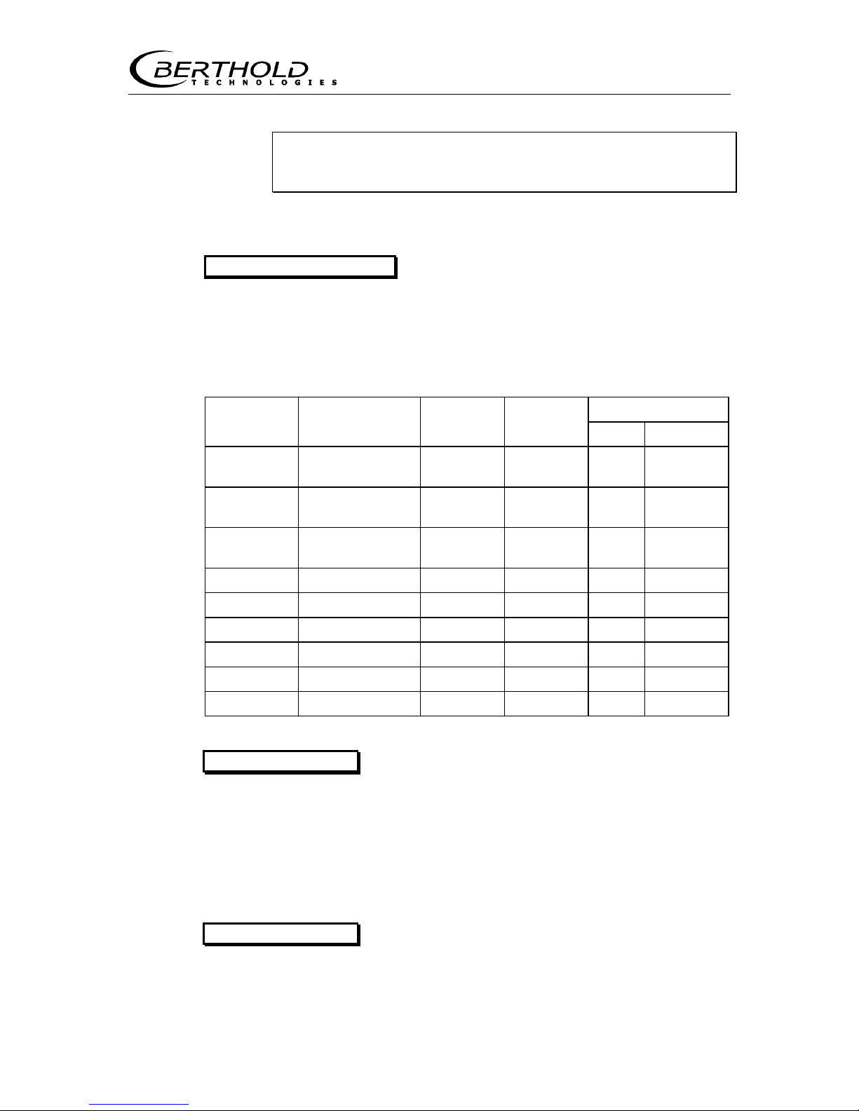
Section 6 Evaluation Unit LB 442
67
The current calibration data is lost when the instrument is
reset!
Measuring Parameter
Detector and Isotope
o Detector code:
Detector-specific code number for automatic high voltage control.
Detector list
Scintillator Type Dimensions
mm
Weight
kg
Operating
code
NaI Plastic
LB 4401-01
LB 5401-01
25/25 6 0
X
LB 4401-02
LB 5401-02
40/35 6 0 X
LB 4401-03
LB 5401-03
50/50 18 0 X
LB 4405-01 500 10 22 X
LB 4405-02 750 10.5 22 X
LB 4405-03 1000 13 13 X
LB 4405-04 1250 13.5 13 X
LB 4405-05 1500 15 10 X
LB 4405-06 2000 22 10 X
Interfaces
Slave 1
(Only if Number of detectors
> 1)
Address for slave 1. We recommend to keep standard address 1.
Further addresses have to be used only when more than 1 slave is
connected. Accordingly, you have to enter the same address in the
slave evaluation unit.
Service Menu
See Service Functions on page 95.
Page 70

7.1 Background
68
Section 7 Calibration
7.1 Background
If you are working with rod detectors, the background, i.e. the
natural environmental radiation, has to be determined. The count
rate of the background has to be regarded as constant and may
therefore not be compensated for automatically. The background
should be measured by placing the detector in a certain distance
from the measuring frame (with Cs137 3 m, with Co60 at least
5 m). If the detector cable is not long enough, a two-wire extension cable may be connected. Before measuring the zero count
rate, the detector has to be in operation or operating voltage has
to be applied for at least 30 minutes.
See also Background for rod detector on page 59.
Note: If the background is not measured correctly, a display deviation may occur in the course of time.
7.2 Tare Measurement
7.2.1 General Information
Before taking the measuring system into operation, the zero or
tare weight has to be determined.
The tare weight changes constantly as a result of conveyor irregularities, such as variation of the thickness of belt or, as in the case
of chain conveyors, differences between chains links and scrapers.
During tare determination, therefore, the conveyor must run and
the average value must be determined over several complete conveyor belt cycles. The rule is: the more cycles, the more precise
the result.
The tare measurement can be checked by running a test measurement with empty belt. During the test measurement (approx. 5
minutes) no or only a negligible mass (t) should be integrated.
There are two ways of performing a tare measurement:
a) Tare measurement via time
b) Tare measurement via belt length
a) Tare Measurement via Time
First, the time for one cycle has to be determined by marking the
belt and taking the time until the mark reappears. With most conveyors, averaging over one belt length is insufficient. For this reason, depending on the available time, enter a multiple of this
value.
Example: 1 cycle measured = 56 s
15 cycles = 840 s
Page 71
Section 7 Calibration
69
b) Tare Measurement via Belt Length
If you know the total belt length (upper and lower belt), you can
run a tare measurement by entering the belt length in meters.
If it is possible to run the conveyor without load for the respective
time, tare measurement can be performed.
At the end of the tare measurement, store the averaged value with
<enter>. If the same count rate is measured again later during
normal operation, the computer knows that the conveyor is empty.
Tare measurement must not exceed 2 hours.
CAUTION! If material is suddenly conveyed during tare
weighing, the result will be falsified. In this case, the tare
measurement has to be started all over again.
Starting the Tare Measurement
Push <run> to start the tare measurement. The tare count rate is
displayed. In addition, if you have selected Time, the remaining
measuring time, if you have selected Length, the remaining belt
length is displayed.
Storing the Tare Count Rate
Push the <enter> button when the measuring time or the belt
length is over to store the tare count rate and the calibration date
(cannot be viewed).
Interrupting the Tare Measurement
The tare measurement can be interrupted and started again any
time by pressing <run> once more.
If a tare measurement has been stopped, the averaged value remains stored and the measurement can be continued any time as
if no interruption had occurred.
However, if you confirm the interruption with <enter>, the tare
count rate is stored together with the calibration date. If you continue the tare measurement with <run>, the count rate is averaged only over the second part of the measurement; i.e. the stored
mean is not taken into account for the further measurement. This
means: if you quit the tare measurement without pushing <en-
ter>, the mean from the first partial measurement is still valid. If
you quit the tare measurement via <enter>, the mean resulting
from the second partial measurement is stored.
External Start of Tare Measurement
The external tare measurement is started and performed automatically by short-circuiting terminals 20a and 20c and the result
is stored with date. For example, if you start an external tare
measurement during measurement, this measurement will be interrupted and the tare measurement started. After the specified
time has elapsed or the belt length is over, the tare count rate and
the calibration date is stored. Then the system returns to the normal operating mode.
Page 72

7.2 Tare Measurement
70
The external tare measurement can also be interrupted or continued again by pressing the <run> button.
Current Output during Tare Measurement
During tare measurement the current output (26a/26c) does not
supply any current (0 mA).
Manual Input of the Tare Count Rate
You may also enter the tare count rate manually. Confirm you entry with <enter>.
Verification and Correction of the Tare Measurement
Check whether the tare value is correct by running the belt without
load for several minutes. During measurement, watch how the
value in the tonnage memory changes. If this change is too big,
you have to repeat tare measurement.
7.2.2 Tare Compensation
All changes occurring in the course of time have to be compensated for by a tare measurement. This includes changes of the
conveyor belt, for example replacement of belts or chains links.
Tare must also be determined again when the belt has been replaced. Recalibration is not necessary.
The same applies if the source is replaced after several years.
If a tare measurement is performed after calibration, all count
rates of the calibration points are converted in accordance with the
new calculated tare count rate. As a result, the calibration curve
remains unchanged, even if it is calculated again with these values.
Therefore, a tare measurement can be carried out any time and
used for correction of the calibration.
Furthermore, one or several calibration points can be added any
time. When adding calibration points, the calibration curve has to
be calculated new (see next section).
Page 73
Section 7 Calibration
71
7.3 Calibration
7.3.1 General Information
Calibration is a correlation of weight and count rate. It should,
therefore, be carried out carefully. The weight is determined with a
comparative weigher. Since any errors of this comparative weigher
will later falsify the results, the weigher should be highly accurate
and preferably a registered one.
Before starting comparative weighing, it is important to find
a way of comparing exactly the same amount of material on
both weighers.
Due to tare determination, we know the first calibration point already: the zero point. The shape of the calibration curve is determined by the position of the calibration points and the calibration
mode. Several points have to be plotted, however, in order to average out measuring errors. At each measurement point, you
should work with a different load. The more the load of a calibration point differs from another calibration point, the better the calibration.
The result of a comparative weighing is an average value of
the weights per area occurring during this time. For this
reason, the accuracy of the curve determination is the better, the more constant the load during weighing!
The evaluation system has space for up to 10 comparative weighings per product.
7.3.2 External Product Selection
If different products or materials with different composition are
conveyed, these products may be calibrated in another menu section. These menu section are called products. External control of
such products is possible via the digital inputs. A maximum of four
different products can be controlled via the digital inputs.
Below we will only describe the calibration for the 1
st
product, since
the procedure for other products is the same.
Page 74

7.3 Calibration
72
7.3.3 Preparation for Calibration Weighing
Required material quantity
At least 20% material of the maximum load is needed for one calibration weighing.
Example: If the measuring range is 0-200 t, at least 40 t material
has to be available for this calibration weighing. For a four-point
calibration 4 times as much material, i.e. 160 t.
In general one can say: the longer a calibration weighing is running, the more accurate the result of the calibration will be. Therefore, calibration weighings are often performed at maximum load,
in our example 200 t. Essentially, however, this is dependent upon
the situation on site.
Unforeseen
Since a calibration weighing is typically performed outside a regular production process, one has to expect that a calibration weighing may often fail for technical or other reasons. For this case,
more material should be prepared.
Comparative weigher
As mentioned above, calibration is a correlation of weight to count
rate. To get a comparative weight, the material has to be weighed
on another pair of scales, i.e. a comparative weigher. Which kind
of comparative weighings are performed is dependent on the situation on site.
- Truck weigher
The material conveyed through the measuring frame is loaded onto
a truck and then moved onto a truck weigher. The truck weigher is
the comparative weigher. Another possibility is to weigh the material prior to calibration and to have it ready for calibration.
- Storage container with weighing cell
The material measured by the measuring frame is conveyed in a
storage container standing on weighing cells.
- Calibration in kg/m
Another possibility is calibration in kg/m. With material that is
moved through the measuring frame as "endless plate", e.g. plates
of 1 m length can be cut out and weighed. While the material is
transported through the measuring frame, the LB 442 averages the
count rate, at the same time the reference samples have to be cut
out. The averaging time should be at least 5 minutes. The comparative weight is calculated from the average value of several
plates and entered in kg/m.
The unit kg/m has to be selected for this kind of calibration. See
also "Select unit" on page 51.
Prerequisite is that the plates always have the same width; otherwise, the measurement has to be performed at different product
calibrations.
Page 75

Section 7 Calibration
73
- Static Calibration
Only a small amount of material is conveyed through the measuring frame for static calibration; this material is/has been weighed
before or after the calibration weighing on a comparative weigher.
This material is conveyed through the measuring frame very slowly
or in small steps. If the material is light, it may be possible to put
it on a foil and to pull it slowly through the measuring frame. If the
weight of the foil it is not negligible, it has to be added to the material weight. While the material is being pulled through the measuring frame, the LB 442 averages the count rate. Pulling the material through the measuring frame should take at least 5 minutes in
order to reduce the statistical error during count rate averaging.
The comparative weight is also entered in kg/m.
The unit kg/m has to be selected for this kind of calibration. See
also "Select unit" on page 51.
Note: A static calibration has to be carried out very thoroughly, as
otherwise the accuracy that can be expected will not be very high.
Again, the longer the averaging time for the count rate, the better.
Page 76

7.3 Calibration
74
7.3.4 Standard Calibration Procedure Step-by-Step
o In the main menu, select sk1: Calibrate and then the submenu
sk2: Calibrate
.
o Select the product (no. 1...10).
o Select the submenu sk1: Data Input
and after the background
for the rod detector, select calibration point 1.
o Load product on conveyor belt and start conveyor belt.
o When the product has reached the measuring frame, push the
<run> button. The computer starts counting the time and aver-
ages the count rate and speed over the measurement.
o If the material used for comparative weighing has passed the
measuring frame, push <run> to stop the measurement. The
averaged count rate and belt speed as well as the measuring
time is displayed.
o If you confirm the 3 values with <enter>, the prompt Com-
parative weight appears.
o Enter result of comparative measurement.
o Confirm value with <enter>.
o Go to next calibration point with <more>. To perform another
comparative weighing, proceed as described, using another data
point in the menu. Measure another calibration point at a differ-
ent load, if possible.
To use no further calibration point, enter „0“ cps at the next
Rate and confirm with <enter>. The values of this and all fol-
lowing calibration points are then not
used for calculation of the
calibration curve.
o Scroll through the calibration points that are not used with
<more>. The display returns to the submenu group sk1: Data
Input/sk2: Calculate.
o Select sk2: Calculate
.
If one imagines these pairs of values, i.e. count rates and calcu-
lated weight per area, plotted on a diagram, we get a line that
connects these points. The computer finds this line automati-
cally. The method used to determine a mathematical function
which provides an optimum connection between these points is
known as regression analysis. Since the plotted curve must be
continuous for physical reasons, not all measuring points will be
on the plotted curve.
One can tell the computer whether it should carry out the re-
gression analysis using a linear
weight per area share, or
whether it should also take into account a cubic
one. See also
curve fit using cubic
coefficients on page 61.
- ln I/Io
x
x
x
x
F
Page 77
Section 7 Calibration
75
Normally it suffices to work with a linear absorption coefficient.
o Select calibration mode lin/squ/cub/auto. Calibration is per-
formed as soon as you confirm the calibration mode with <en-
ter>.
o Then you can call the results with <more>: depending on the
selected calibration mode: a
1
describes the linear, a2 the square
and a
3
the cubic coefficient.
o You may use the square error to assess the quality of the calcu-
lated calibration curve. If this value is greater than 10
-4
, the
calibration is not OK.
If more than three calibration points are used, we recommend to plot a x/y graph. The weight per area is plotted on
the y axis and the logarithmic value of the count rate on the
x axis. The visual presentation of the calibration allows a
very good assessment of the quality of the calibration and is
very helpful in trouble-shooting the calibration.
Page 78

8.1 General Information
76
Section 8 Checking the Calibration
8.1 General Information
If deviations of the measured result occur, a new tare measurement has to be performed first. To carry out a performance check
of the bulk flow measurement, you can push a calibration cap (option) over the scintillator. The load measured at empty belt with
the calibration cap must not change compared to previous tests,
provided the calibration coefficients did not change in the meantime.
8.1.1 Correction of Calibration
First, you should run a tare measurement and a check as described
in Section 8.
If you detect any deviations, you may correct the slope of the
curve by a multiplicative factor (see Correction of Display Value on
page 77).
8.1.2 Operating Instructions for Calibration
Start and Stop of Calibration Measurement
Push the <run> button to start and stop a calibration measurement. With <+> and <-> you can switch to the live display. In the
live display, a push of the <run> button is ignored. With the <+>
and <-> buttons you can scroll in this window; the current, not yet
calibrated measured values are displayed. With <more> you get
back to the calibration window.
Store
When the calibration measurement has been stopped, confirm the
respective measured value with <enter>; otherwise it will be rejected when exiting the respective ‘calibration point’.
Stop Measurement
If the system is in the operating mode, the ongoing measurement
can be stopped by pushing the <run> button, provided the measurement product is the same as the calibration product. If the selected product is not the same as the measurement product, the
<run> button is locked. The calibration parameters for the selected product can only be entered manually.
Current Output
The current output supplies a current proportional to the load and
the selected measuring range, provided the correct absorption coefficient has been entered.
Page 79

Section 8 Checking the Calibration
77
Which Calibration Points are Calculated?
The evaluation computer calculates the calibration curve (absorption coefficients) from the measured values. All calibration points
are used for this calculation where the parameters count rate,
speed, measuring time and comparative weight contain valid values (> zero). When entering invalid parameters or if invalid parameters (zero) are present, the respective calibration point is not
taken into account in the calculation. All unused calibration points
should be deleted.
8.2 Correction of Display Value
This option should not be regarded as a substitute for a careful
calibration. It should only be used if minor corrections are required
when in the load display. Otherwise we recommend to run a recalibration.
An additive constant can be entered at Offset, a multiplication factor at Factor (Calibrate menu, submenu Calculate).
8.2.1 Offset
The value stored under Offset is added to the load. This allows a
parallel offset of the calibration curve. This means an offset of the
tare value. We recommend using the factor to correct the display
value.
8.2.2 Factor
The load is multiplied by the value stored as Factor. This allows
you to change the gradient of the calibration curve.
Formula
The display value is calculated as follows:
Display (t/h) = Factor x Measured value (t/h) +
Offset
Measured value (t/h): Calculated load using the current count
rate without taking into account factor and offset.
Page 80

9.1 Live Display
78
Section 9 Operation of the Radiometric
Bulk Flow Meter
9.1 Live Display
Start measurement: Push <run> button
Result display (Live display):
Load t/h, kg/h
Totalizer (t or kg)
Dry Totalizer (t or kg)
Moisture %
Act. Speed m/s
Live Curr. mA
Live cps
Tare cps
Det. temp. °C
Scroll in live display
: <+>- or <-> button.
Stop measurement:
Push <run> button once more.
9.2 Regular Operation
9.2.1 Results
During measurement, the current conveyor load is displayed, the
total tonnage is integrated in the mass integrator over the entire
measuring time. The mass integrator can be set via the option
Erase mass integrator yes/no in the Measuring Parameter
menu so
that is cleared after each run.
During measurement operation, the mass integrator can be reset
to zero any time with the <clear> button.
The printout can be made as minute or shift printout.
Page 81

Section 9 Operation of the Radiometric
Bulk Flow Meter
79
Minute printout
Minute: 13/08/97 13:16 P1 Weight[t] 3.617 Diff[t] 0.032
Minute: 13/08/97 13:17 P1 Weight[t] 3.661 Diff[t] 0.022
Minute: 13/08/97 13:18 P1 Weight[t] 3.680 Diff[t] 0.013
Minute: 13/08/97 13:19 P1 Weight[t] 3.699 Diff[t] 0.029
Minute: 13/08/97 13:20 P1 Weight[t] 3.725 Diff[t] 0.031
Minute: 13/08/97 13:21 P1 Weight[t] 3.710 Diff[t] 0.024
etc.
Shift printout
Hour: 13/08/97 07:00 P1 Weight[t] 3793.617 Total [t] 3793.617
Hour: 13/08/97 08:00 P1 Weight[t] 3855.234 Total [t] 7648.851
Hour: 13/08/97 09:00 P1 Weight[t] 3639.364 Total [t] 11288.215
Hour: 13/08/97 10:00 P1 Weight[t] 3868.222 Total [t] 15156.437
Hour: 13/08/97 11:00 P1 Weight[t] 3697.430 Total [t] 18853.867
Hour: 13/08/97 12:00 P1 Weight[t] 3894.555 Total [t] 22748.422
Hour: 13/08/97 13:00 P1 Weight[t] 3633.837 Total [t] 26382.259
Hour: 13/08/97 14:00 P1 Weight[t] 3793.943 Total [t] 30176.202
Shift: 13/08/97 14:00 P1 Weight[t] 30176.202Total [t] 30176.202
etc.
9.2.2 Zero Point Correction through Tare Measure ments
In addition to the on-going measurement which is displayed live,
the tare measurement is also part of normal operation.
All changes occurring with time must be compensated for by a tare
measurement. In particularly, this includes changes on the belt itself. A deposit layer may also form on the belt depending on the
material being conveyed. The user must decide how often the tare
weight should be measured. The button must only be pressed
when the belt is absolutely empty, everything else is done automatically. We recommend checking the tare once a month.
Tare must also be determined again when the belt has been replaced. Recalibration is not necessary.
The same applies if the source is replaced after years (see section
Radiation Protection Guidelines when this should be done).
No
tare measurement is necessary to compensate for the natural
decay of activity. Since the computer also contains a clock (Date &
Time in the General Data
menu), this change can be compensated
for mathematically. It takes place every night exactly at midnight.
You can check this as well. After several days the tare count rate
changes automatically. If the computer has been without power
supply for some time, the clock is supplied with power by a battery. At the next measurement, the decay compensation is corrected automatically.
Page 82

9.3 Operation with Different Materials
80
9.2.3 Batch Operation
In addition to weighing the conveyed material continuously, the
bulk flow measurement can also be used for batch weighing. This
operation mode allows, for example, to load trucks with a given
amount, or to control a feeding machine.
The following settings are required:
o In the Measuring Parameter
menu, select the product being
measured.
o In the Measuring Parameter
menu, select as Operating Mode the
mode Batch via keyboard or Batch via external.
o In the I/O Config.
menu, select Clear Ext. Batch Start/Mass In-
tegrator for Digital Input 1 if you want to perform an external
batch measurement.
o In the I/O Config.
menu, select Batch Ready for Digital Output
relay 3 and then enter the batch weight.
If the preset batch has passed through the measuring frame, a
signal is triggered at digital output relay 3 that can be used, for
example, to turn off the belt.
Another batch measurement can be carried out.
9.3 Operation with Different Materials
If various products requiring different calibrations are to be conveyed, you have to run separate calibrations for each product
(max. 10 different products).
The product can be selected either via keyboard by entering the
product number in the Measuring Parameter
menu, item Measuring
Product. External selection is possible only for 2 different products
via digital input 3 (open = product 1, closed = product 2).
In the print protocol, the products are identified by the labels P1,
P2 ... P10.
Page 83
Section 9 Operation of the Radiometric
Bulk Flow Meter
81
9.4 Evaluation Unit as Dry Weight Computer
The evaluation unit includes an input for moisture compensation
(28a/28c). If a moisture probe is connected and moisture compensation is activated (menu Operating
mode, Config Instrument:
moisture compensation), the measured wet weight is computed
with the measured moisture value and one gets the dry weight.
With activated moisture compensation, the dry weight and the total weight is indicated on the display.
9.5 Starting/Stopping Operation of the System
To stop operation of the measuring system, proceed as follows:
Disconnect system from mains.
Lock radiation exit channel of shielding container and secure lock-
ing handle with lock.
Use water cooling if the temperature of the detector is likely to rise
above 50°C even though the instrument is not in operation.
With sub-zero temperatures, empty the water cooling.
To start operation of the measuring system:
Open radiation exit channel
Power on the instrument.
Put water cooling in operation again, if it was disabled.
Page 84

9.6 Error Messages
82
9.6 Error Messages
9.6.1 Resetting Error Messages
a) All error messages must be reset with <enter>.
b) Several simultaneously or consecutively occurring errors are
stored in an error register in the order of their appearance; they
have to be reset individually by operating <enter> several
times.
c) All errors are signaled via the “Error” output (Relay 16a/16c).
9.6.2 Error Messages during Operation
Error
No.
Error text Cause Solution
10
Not calibrated
No calibration coefficient
available or not calculated
- Enter coefficient or calculated it
11
Power fail
>1 month – time?
The date has changed since
the last operation by one
month
- Check date
- Battery still OK?
12
No input allowed
Device locked by password - Enter password
32
Wrong password
Wrong password entered - Enter correct password
34
Wrong input
Wrong parameter entered - Input lies outside range
39
Time constant 1
< 1s
Time constant 1 too small - Input value has to be > 1
40
Time constant 2
< 1s
Time constant 2 too small
- Input value has to be > 1
47
Check external mass
counter setting
Input is outside the limits
and is ignored.
(triggered when changing
parameters – measuring
range or mass counter)
- Increase step-width of mass
counter or reduce maximum
measuring range
(safety circuit, so relay output
can still follow)
Page 85

Section 9 Operation of the Radiometric
Bulk Flow Meter
83
9.6.3 Error Messages during Calibration
Error
No.
Error text Cause Solution
10
Not calibrated
No calibration coefficient
available or not calculated
- Enter coefficient or calculated it
38
Wrong product
If the product is unequal to
the calibration product when
reading-in the calibration
count rate
- Adapt product to calibration
product
41
min. measuring range not
reached
Enter negative measuring
range
- Check final value
(only with square or cubic curve)
42
max. measuring range
exceeded
Measuring range input lies
above the limit
- Check final value
(only with square or cubic curve)
43
Rate Overflow
With twisted measuring
range
- Check input
47
Check external mass
counter setting
Input is outside the limits
and is ignored.
(triggered when changing
parameters – measuring
range or mass counter)
- Increase step-width of mass
counter or reduce maximum
measuring range
(safety circuit, so relay output
can still follow)
9.6.4 Error Messages during Measurement
Error
No.
Error text Cause Solution
1
Rate Overflow
Count rate >520.000cps
- Check configuration of application, or calculation
2
No Detector Rate
Error in detector - Error in detector
- Multiplier or probe electronics
faulty
3
Wrong HV
HV < 500V or >1500V, outside the control range
- Error in detector
- Multiplier or probe electronics
faulty
6
Detector temperature >
65°C
Detector temperature has
exceeded 65°C
- Detector too warm, provide
adequate cooling
7
Trouble with detector
communication
Data transfer between detector and evaluation unit
faulty
- Check connection terminals of
cable
- Detector or evaluation unit
faulty
- Broken cable
9
Detector temperature >
85°C
Detector temperature has
exceeded 85°C
- Detector too hot, provide adequate cooling
44
Current input error
Input current above 23 mA - Check power source
46
Check external mass
counter setting
Input is outside the limits
and is ignored.
(triggered when changing
parameters – measuring
range or mass counter)
- Increase step-width of mass
counter or reduce maximum
measuring range
(safety circuit, so relay output
can still follow)
Page 86

10.1 Evaluation Unit LB 442
84
Section 10 Technical Data
10.1 Evaluation Unit LB 442
Versions: LB 442-1 Master system
LB 442-2 Slave system for detector connection to
multi-detector configurations. Signal transfer to master system via RS 485
Assembly: 19" module 3 HE, 21 TE; Protection type IP 20
Power supply: 115 V ± 10% AC
230 V ± 10% AC
18 to 32 V DC
24 VAC
Observe label on instrument backpanel.
Power consumption: approx. 30 VA or 30 W
Temperature range: Version 19“ frame
Operating temperature: 0 to +50 °C; no condensation
Version Wall Housing LB4460
Operating temperature: 0 - 40 °C; no condensation
Storage temperature: -40 to +70 °C
CPU: 32 bit computer.
Data storage in FLASH memory.
Weight: approx. 2 kg
Display: LCD display with 4 x 20 characters, illuminated.
Data input via keyboard.
Softkey guided dialog,
Languages: German, English, French and Spanish.
Data manipulation possible only after password entry.
Interfaces: RS 232 and RS 485
Time constant: 0.5 - 999 s with automatic reduction to 1/10 of the
value in case of rapid measured value changes (can
be switched off). Trigger threshold for time constant
switch-over adjustable.
Decay comp.: Automatic for
137
Cs, 60Co,.
241
Am, 85Kr,
244
Cm, 90Sr
Page 87

Section 10 Technical Data
85
Inputs/Outputs:
Detector terminal: (2a/2c)
II 2 G [EEx ib] IIC or II 2 G [EEx ib] IIB
The table below shows the highest permissible external
inductivity and capacity:
II 2 G [EEx ib] IIC II 2 G [EEx ib] IIB
Highest permissible external inductivity
0.15 mH 1.8 mH
Highest permissible external capacity
344 nF 507 nF
The effective inner inductivity is negligible.
Effective inner capacity: 12 nF
For inherently safe installation, the cable ends on the
strip terminal must be protected by a 10 mm long
shrink-down plastic tubing (see also the connection
diagram)
3 digital inputs: passive
1. Belt stop or erase mass integrator (18a/18c)
2. External start tare measurement or print start,
Product 3+4 and Start/Stop and print (20a/20c)
3. External product selection (22a/22c)
Current output: for Load 0/4 - 20 mA isolated (max. 500 Ω)
(26a+/26c-)
Limit value outputs: Relay 2: (12a/12c): Mass counter (pulse length 25 to
450ms, default setting 50ms) Relay 3 (14a/14c): Tare
measurement or Batch Ready or Min/max
Relay 1: (16a/16c): Failure alarm
Loading capacity: at resistive load
AC: Max. 250V, max. 1A, max. 200VA
DC: Max. 300V, max. 1A, max. 60 W
Current input: 0/4 - 20 mA (28a-/28c+)
Speed or moisture
Pulse input: (28a-/28c+)
Pulse tachometer (500 pulses/rev, 2500 pulses/rev,
5000 pulses/rev)
Interfaces: RS 232 on instrument front panel
Port for data transfer from evaluation unit to printer or
PC.
Page 88
10.2 Detector
86
10.2 Detector
The probe is designed for industrial application. It in-
cludes a scintillation counter for Gamma radiation
which is equipped with a NaI crystal or plastic scintillator. The built-in microprocessor defines the configuration, counts the pulse rates, controls the high voltage, measures the temperature of the probe and an
external Pt 100, transfers data and performs calibration and control functions. Power supply and communication take place via 2-wire technology. The probe is
ex-protected and is licensed for:
LB 44X1 : Scintillation counter with NaI (Tl) crystal 25/25, 40/35
or 50/50.
Stability : ± 0,1 %
Protection types according to ATEX:
II 2 G EEx de IIC T6
II 2 G EEx ib d II C T6
Type EX Crystal
size
mm
Weight
kg
Detector
code
LB 4421-02 X 40/35 18 0
LB 4401-03 X 50/50 18 0
LB 4405 : Scintillation counter with plastic scintillator,
long-term stability ±1 %,
sensitive lengths see table below.
Protection types according to ATEX:
II 2 G EEx de IIC T6
II 2 G EEx ib d II C T6
See also Atex Certificates on page 115.
Rod detectors with plastic scintillator
Type
Sensitive
length mm
Weight in
Kg
Detector
code
LB 4405-01W 500 11.5 22 (24)
LB 4405-02W 750 14 22 (24)
LB 4405-03W 1000 17 13 (15)
LB 4405-04W 1250 19.5 13 (15)
LB 4405-05W 1500 22 10 (12)
LB 4405-06W 2000 25 10 (12)
Page 89
Section 10 Technical Data
87
Detector code in () can be used to reduce the back-
ground. Any change in the detector code requires a
new calibration.
LB 54X1 : Scintillation counter with NaI (Tl) crystal 25/25, 40/35
or 50/50.
Stability : ± 0,1 %
without Ex
Type Crystal size
mm
Weight
kg
Detector
code
LB 5421-02 40/35 18 0
LB 5401-03 50/50 18 0
LB 5481-06 44/5 4 (1) 7*
* Detector code 7, valid from detector software 1.02
(delivery date Feb. 2000)
Protection type: IP 65.
Housing: Stainless steel housing.
Cable entry: M16 for external cable diameter 7...11 mm.
Scintillators: NaI (Tl) crystal
Size: 25*25mm, 50*50mm, 40*35mm, 44*5 mm.
Stability : ± 0,1 %
Photomultiplier: EMI
HV generation: Voltage range control 500 V to 1500 V
Counter: Rate max. 524 000 CPS
Temp. measurement: via NTC, accuracy: ±3°C
Operating temp.: - 40 to + 60°C. For point detectors
- 40 to + 55°C. For point detectors
A water cooling device is available for higher temperatures.
Monitoring of detector temperature and alarm when
exceeding the max. permissible temperature.
Storage temp.: -50 to + 70°C for point detectors
-50 to + 55°C for rod detectors
Input voltage: +11 to16 V DC
Power consumption: Typically 60 mA Max. 90 mA
Feed voltage: Typically 13.6 to 14.1 V
Housing sealing: IP65
Screwed cable gland: M16, external cable diameter: 6 to 10 mm
Cable e.g. 2 * 1 square, outside: 6.3 mm (Ölflex 110 blue)
Cable resistance, 2-wire: 39 Ohm/km
or
2 * 1.5 square: 26,6 Ohm/km
2 * 2.5 square: 16 Ohm/km
Page 90
10.3 Wall Housing LB4460
88
Permissible cable
resistance: 29 Ohm (for wire and return wire)
Connection cable: Two-wire.
Max. cable length : 750 m (13.6 V applied current, 90 mA, 1 square)
1 km ( 1.5 square, connection box required)
1.8 km ( 2.5 square, connection box required)
Cross section
in mm²
Max. cable length
in m
1 750
1.5 1000
2.5 1800
10.3 Wall Housing LB4460
Protection types: ATEX:
II 2 G EEx ib IIC
II 2 G EEx ib IIB
Ambient temperature with protection type ATEX:
Depending on the number of installed evaluation units
installed
evaluation units
Max. ambient
temperature
2 40°C
1 45°C
See also ATEX Certificate for Wall Housing on page
124.
Protection type: IP 65
Housing: Polyamide housing.
Page 91

Section 11 Service Instructions
89
Section 11 Service Instructions
11.1 General Safety Precautions
Any time you are working on electrical components, you have to
observe the relevant safety regulations. Please refer to the GENERAL WARNINGS and SPECIFIC WARNINGS in the Safety Summary.
Any work in the direct vicinity of the shieldings containing
the radioactive source may be performed only following
proper training and/or professional guidance. Please see
SPECIFIC CAUTIONS in the Safety Summary.
11.2 Trouble Shooting
Problem Possible Cause Potential Solution
No display No power supply Check mains cables
Check fuses
Display unreadable Processor error Note error code
Perform total reset
Replace evaluation unit
No pulse rate
(Error code 2)
Power supply for detector interrupted
Check cable to detector
Detector is faulty Replace detector
Pulse rate too low Shielding not open or
not properly opened
Check lock and secure it in position
OPEN
Alignment of useful
beam toward detector
not correct
Correct and optimize alignment
Source has reached the
end of its service life
Renew source (Co-60 after 5 to 10
years, at the earliest)
No or incorrect result reading
Entry of calibration values incorrect
Check calibration values
Output current incorrect
Entry of calibration values incorrect
Check calibration values
Result reading fluctuates strongly
Time constant too small Increase time constant in the
Measuring Parameter menu (min
20 s)
Pulse rate too low Check age of source and irradiation
level. Replace detector
Result reading
shows drifts
Detector stabilization
faulty
Replace detector
Photomultiplier faulty Replace photomultiplier
Page 92
11.3 Shielding and Source
90
11.3 Shielding and Source
The shieldings do not include any wearing parts or mechanically
moving parts that under normal operating conditions require maintenance. For safety reasons, however, it should be possible any
time to lock the useful beam.
A function check has to be performed in appropriate intervals of half a year. The Radiation Safety Officer has to be informed immediately if any faults on the shielding or a sluggish locking mechanism are detected.
If the problem cannot be solved by simple measures such as cleaning, stop working with the system until it has been repaired.
As long as the shielding does not show any significant mechanical
damage or strong corrosion, the built-in source will be protected.
Refer to the Radiation Protection Guidelines in Section 12 to check
or replace the source.
The radioactive source used and the measuring system have a service life of 5 to 10 years. A source has to be replaced when statistical variations which increase in the course of time become intolerably high and any compensation by increasing the time constant
is not permitted, e.g. due to control engineering reasons.
A tare measurement has to be performed any time a source
is replaced!
For information on the design of source and shielding see the technical documentation and the identity plate (Figure 31).
Source No. :
1234 - 11- 94
MBq Co-60
400
Shielding
mm
Date
12.11.94
Pb
98
Dose rate in 1 m distance
5
µµµµ
Sv/h
MODEL LB 7440
Bad WildbadD-75323
Figure 31: Identity plate
Page 93

Section 11 Service Instructions
91
If the source has to be renewed, you have to specify the manufacturing number of the original source in your new order. This manufacturing number consists of three groups of digits, for example:
1234 - 11 - 97
The first group is a consecutive number, the second group identifies the month (here: November) and the third the year the source
was manufactured (here: 1997). It is included on the identity plate
of the shielding and also on the leak test certificate that comes
with every source.
Page 94

11.4 Evaluation Unit LB 442
92
11.4 Evaluation Unit LB 442
After power on, the instrument identification must appear on the
display and with <more> you go on to the operating parameters
of the various menu structures. If no entry is made, the program
automatically switches from the current menu to the display mode
after a few minutes.
The evaluation unit includes an error monitoring device which also
covers the detector functions and displays error codes indicating
instrument faults. For information on the error and the potential
cause see the Error Code Listing. If a hardware error occurs, the
evaluation unit has to be replaced.
If no error code is displayed, this means that the electronics is
working correctly and all measured values and parameters are
within the normal range. Possible function problems must then
have another cause. Please refer to the 11.2 Trouble Shooting.
A total reset should be performed only in exceptional cases and after consultation with Berthold Technologies
A total reset is performed by pressing the Clear key – while the instrument is turned off – and turning the instrument on at the same
time.
11.4.1 Battery
If the computer is without power supply (power down or separated
from mains), the clock is supplied with power by a battery. No decay compensation is performed during this time. This will be done
as soon as the evaluation unit is connected to mains. Decay compensation is performed when the date changes.
The service life of the battery, even in case of continuous stress,
i.e. when the evaluation unit is not connected to mains, is 7 years.
Battery Type:
VARTA
CR 2032
3V 220mAh
Page 95

Section 11 Service Instructions
93
11.4.2 Error Code Listing
No.
Error text Cause Solution
1
Pulse rate overflow Pulse rate > 520,000 cps - Check configuration of application, or
calculation
2
No pulses from
detector
Fault in detector Error in detector
-Multiplier or probe electronics faulty
3
HV wrong HV < 500V or >1500V, outside
controlled range
- Error in detector
-Multiplier or probe electronics faulty
5
Measuring range
for current output
0/4-20mA faulty
Upper limit is smaller or equal to
lower limit (triggered during calibration calculation)
- Check measuring range input
6
Detector temperature > 65°C
Detector temperature has exceeded 65°C
- Detector too warm, provide adequate
cooling
7
Trouble with detector communication
Data transfer between detector
and evaluation unit faulty
- Check connection terminals of cable
-Detector or evaluation unit faulty
-Broken cable
9
Detector temperature > 85°C
Detector temperature has exceeded 85°C
- Detector too hot, provide adequate
cooling
10
No calibration No calibration coefficient available
or not calculated
- Enter or calculate coefficient
11
Power fail
>1 month – time?
The date has changed since the
last operation by one month
- Check date
-Battery still OK?
12
No input allowed Instrument locked by password - Enter password
32
Wrong password Wrong password input - Enter correct password
34
Wrong input value Wrong parameter entry - Input lies outside range
35
Calibration error Parameters for calculation of cali-
bration curve are missing
- Check absorption coefficient and tare
38
Wrong product Measurement product is not the
same as product while reading the
calibration count rates
- Adapt product to calibration product
39
Time constant 1
< 1s
Time constant 1 too small - Input value has to be > 1
40
Time constant 2
< 1s
Time constant 2 too small - Input value has to be > 1
41
min. measuring
range not reached
Enter negative measuring range - Check final value
(only with square or cubic curve)
42
max. measuring
range exceeded
Measuring range input lies above
the limit
- Check final value
(only with square or cubic curve)
43
Rate Overflow With twisted measuring range - Check input
44
Current input error Input current above 23 mA - Check power source
46
Check external
mass counter setting
Input is outside the limits and is
ignored.
(triggered when changing parameters – measuring range or mass
counter)
- Increase step-width of mass counter or
reduce maximum measuring range
(safety circuit, so relay output can still
follow)
47
Check external
mass counter setting
Input is outside the limits and is
ignored.
(triggered when changing parameters – measuring range or mass
counter)
- Increase step-width of mass counter or
reduce maximum measuring range
(safety circuit, so relay output can still
follow)
Page 96
11.4 Evaluation Unit LB 442
94
11.4.3 Error Code Listing with Signal Output
No.
Error text
In case of error,
measurement:
Alarm
Relay
0/4 -
20mA
ABORT CONTINUE
1
Pulse rate overflow abort continue alarm value
2
No pulses from detector stop continue alarm value
3
HV wrong abort continue alarm value
5
Measuring range for current
output 0/4-20mA faulty
abort continue no alarm normal
6
Detector temperature > 65°C continue continue alarm normal
7
Trouble with detector
communication
abort abort alarm value
9
Detector temperature > 85°C abort abort alarm value
10
No calibration abort abort no alarm hold
11
Power fail
>1 month – time?
abort continue alarm value
12
No input allowed continue continue no alarm normal
32
Wrong password continue continue no alarm normal
34
Wrong input value continue continue no alarm normal
35
Calibration error abort abort no alarm hold
38
Wrong product abort abort no alarm normal
39
Time constant 1 < 1s continue continue no alarm normal
40
Time constant 2 < 1s continue continue no alarm normal
41
min. measuring range not
reached
abort abort no alarm normal
42
max. measuring range exceeded
abort abort no alarm normal
43
Rate Overflow continue continue no alarm normal
44
Current input error abort continue alarm normal
46
Check external mass counter
setting
abort abort alarm value
47
Check external mass counter
setting
continue continue alarm value
Page 97
Section 11 Service Instructions
95
11.4.4 Service Functions
The service menu structure shows the possible test settings and
switch functions. In addition to defaulted pulse rates that are used
to check the output current, you can check the relay and external
switch functions, and start an automatic plateau recording of the
NaI crystal-multiplier assembly. The result can be read out from
the plateau recording submenu and plotted as a curve.
Moreover, you can preset the high voltage for the detector or turn
off the automatic high voltage control. In another menu you can
calibrate the D/A-converter to the exact output current.
See also Service Menu on page 150.
Test calculation :
Test cps
You can enter any pulse rate within the calibration range to simulate an output current and the weight per area.
Result output
The output current and the respective weight per area is displayed
as a result of the defaulted pulse rate
I/O Test
Curr. Output
You can set any output current within the range.
To test the connected instruments and the current output, you can
set any output current between 0 and 22 mA .
Curr. Input
Shows the current measured at the current input . The input can
be checked using a test power source.
Relay 1/2/3
The relays can be switched to test the signal circuits.
Input 1/2/3
Shows if the inputs are open or closed.
Page 98
11.4 Evaluation Unit LB 442
96
HV Settings
Set detector HV
With the standard setting ”0” the detector works with automatic
high voltage control. For service purposes, you can enter a high
voltage value between 500 V and 1500 V. In this case, the high
voltage control is disabled. The voltage control applied at the photomultiplier then corresponds to the entered value.
For the regular measurement mode you have to enter 0.
Save default
Here you can enter a high voltage start value. This allows rapid
control of the HV to the optimum operation point after power outage. The value can lie between 500 V and 1500 V.
Read default
The start value of the high voltage stored in the detector is displayed here.
Status request
o Temp.PT100
The PT 100 temperature is displayed.
o NTC-Temp.
The temperature in the detector is displayed.
o Pulses
The current count rate of the detector is displayed.
o HV
The currently set high voltage is displayed
Reset Detector
A reset on the detector CPU can be carried out.
Pt 100 Adjust
With a 100 Ohm resistance at terminals 3/4 of the detector, the
PT100 input can be adjusted with the button combination "sk2 &
clear".
Page 99
Section 11 Service Instructions
97
Plateau
Start Plateau
You can automatically measure a plateau of the detector in steps
of 60 V, e.g. to check the correct function of the NaI crystalmultiplier combination.
Check Plateau
The value pairs of the plateau measurement can be displayed here
and plotted as a curve for evaluation.
Adjust current i/o.
Adjust current out
Adjust current output to the values 1.8 mA
and 18 mA by increas-
ing or reducing the numerical value on the display.
Adjust current in
Calibration of current input. Feed current of 1.8 mA. Confirm display with <enter> and go on with <more>.
Then feed current of 18 mA, confirm with <enter> and go on with
<more>.
Note: The current input calibration is omitted when the test input
is configured as pulse input. In this case, this input is used as
pulse input.
Relay delay
Defining the length of a pulse at the external mass counter pulse
output. Standard setting is 50 ms. The setting range is between
10 ms and 440 ms.
Operating time
The date and time of power failure are documented, providing information on power failure and service life.
Page 100

11.5 Scintillation Detector
98
11.5 Scintillation Detector
Scintillation counters do not include any wearing parts and their
service life is not limited, provided they are used under normal operating conditions. Malfunctions in the scintillation detector can
only be caused by excessive mechanical or thermal stress. The
transfer of heavy vibrations or shocks to the detector has to be
prevented by suitable measures, such as separate installation or
shock absorbers. Moreover, with temperatures of above 50°C at
the installation site, heat shields or water cooling devices have to
be foreseen for the detector.
11.5.1 Working Principle
The scintillation counter comprises:
a) sodium iodide crystal doped with Thallium
b) photomultiplier
c) electronics unit.
As the gamma radiation hits the detector, it triggers minute
flashes of light in the crystal which are invisible to the naked eye.
These flashes of light release electrons from the light-sensitive
cathode (photo cathode) of the photomultiplier. This electron current is amplified via a dynode system resulting in an electrical impulse at the photomultiplier output for each impinging light flash.
In the electronic unit connected to the photomultiplier output these
pulses are amplified and counted and the result is transmitted as
digital information via two-wire cable.
The high voltage for operating the photomultiplier is generated in
the electronic unit. The connecting cable between evaluation unit
and scintillation counter only carries a direct voltage and the
measuring signal.
The scintillation counter is equipped with a drift compensation
which compensates for the effects of aging and temperaturerelated gain variations, thus ensuring high long-term stability.
 Loading...