

Page 1

Engineer-to-Engineer Note EE-218
a
Technical notes on using Analog Devices DSPs, processors and development tools
Contact our technical support at dsp.support@analog.com and at dsptools.support@analog.com
Or vi sit our o n-li ne r esou rces htt p:/ /www.analog.com/ee-notes and http://www.analog.com/processors
Writing Efficient Floating-Point FFTs for ADSP-TS201 TigerSHARC®
Processors
Contributed by Boris Lerner Rev 2 – March 4, 2004
Introduction
So, you want to write efficient code for the
ADSP-TS201 TigerSHARC® processor? Or,
maybe, you have come across the optimized
example floating-point FFT for this processor
and would like to understand how it works and
what the author had in mind when writing it.
This application note tries to answer both
questions by going through that FFT example
and all its levels of optimization in detail. This
example can be followed in developing other
algorithms and code optimized for the ADSPTS201S processor.
Generally, most algorithms have several levels of
optimization, all of which are discussed in detail
in this note. The first and most straightforward
level of optimization is paralleling of
instructions, as the processor architecture will
allow. This is simple and boring. The second
level of optimization is loop unrolling and
software pipelining to achieve maximum
parallelism and to avoid pipeline stalls. Although
more complex than the simple parallelism of
level one, this can be done in prescribed steps
without good understanding of the algorithm and,
thus, requires little ingenuity. The third level is
to restructure the math of the algorithm to still
produce valid results, but so that the new
restructured algorithm fits the processor’s
architecture better. Being able to do this requires
a thorough understanding of the algorithm and,
unlike software pipelining, there are no
Copyright 2004, Analog Devices, Inc. All rights reserved. Analog Devices assumes no responsibility for customer product design or the use or application of
customers’ products or for any infringements of patents or rights of others which may result from Analog Devices assistance. All trademarks and logos are property
of their respective holders. Information furnished by Analog Devices Applications and Development Tools Engineers is believed to be accurate and reliable, however
no responsibility is assumed by Analog Devices regarding technical accuracy and topicality of the content provided in Analog Devices’ Engineer-to-Engineer Notes.
prescribed steps that lead to the optimal solution.
This is where most of the fun in writing
optimized code lies.
In practical applications it is often unnecessary to
go through all of these levels. When all of the
levels are required, it is always best to do these
levels of optimization in reverse order. By the
time the code is fully pipelined, it is too late to
try to change the fundamental underlying
algorithm. Thus, a programmer would have to
think about the algorithm structure first and
organize the code accordingly. Then, levels two
and one (paralleling, unrolling, and pipelining)
are usually done at the same time.
The code that this note refers to is supplied by
Analog Devices in the form that allows it to be
called as either a real or a complex FFT, the last
calling parameter of the function defining if real
or complex is to be called. The real N-point FFT
is obtained from the complex N/2-point FFT with
an additional special stage at the end. This note is
concerned with code optimization more than the
technicalities of the special stage, so it discusses
the algorithm for the complex FFT portion of the
code only. The last special stage of the real FFT
is discussed in detail in the comments of the
code.
Standard Radix-2 FFT Algorithm
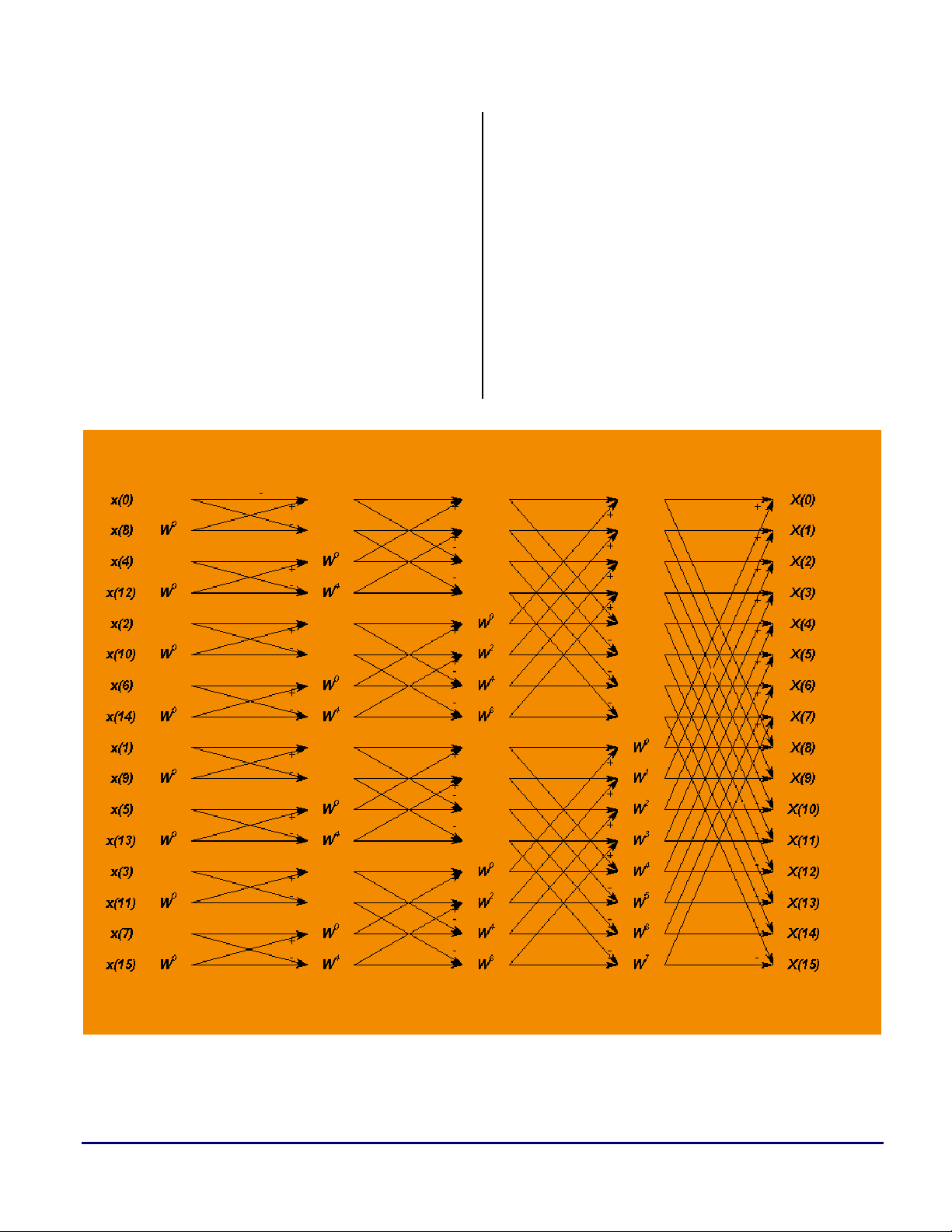
Figure 1 shows a standard 16-point radix-2 FFT
implementation, after the input has been bitreversed. Traditionally, in this algorithm, stages
Page 2
a
1 and 2 are combined together with the required
bit reversing into a single optimized loop (since
these two stages require no multiplies, only adds
and subtracts). Each of the remaining stages is
usually done by combining the butterflies that
share the same twiddle factors together into
groups (so the twiddles have to be fetched only
once for each group). Un-optimized assembly
source code for a TigerSHARC processor
implementing this algorithm is shown in Listing
1. This, with a few tricks that are irrelevant to
this discussion, is the way that the 32-bit
floating-point FFT code was written when it was
targeted to an ADSP-TS101 processor. The
benchmarks (in core clock cycles) for this
algorithm, including bit reversal, running on an
ADSP-TS101 and ADSP-TS201, are shown in
Table 1. Note that since the ADSP-TS101 has
less memory per memory block than a ADSPTS201, larger point size benchmarks do not
apply to the ADSP-TS101. Clearly, as long as
the data fits into the ADSP-TS201 cache, it is
efficient. Once the data becomes too large for the
cache, this FFT implementation becomes
extremely inefficient – the cycle count increases
from optimal by a factor of five.
Figure 1. Standard Structure of the 16-Point FFT
Writing Efficient Floating-Point FFTs for ADSP-TS201 TigerSHARC® Processors (EE-218) Page 2 of 16
Page 3
//*********************************** Stages *************************************
k10 = k31 + N;; // twiddles stride
k11 = k31 + N/2;; // butterflies/group
j12 = j31 + 1;; // groups
j10 = j31 + 2;; // width of butterfly
j11 = j31 + 4;; // butterfly stride
k20 = k31 + STAGES;;
_stages_loop:
j0 = j31 + j29;; // j0 -> internal_buff
k0 = k31 + k30;; // k0 -> twiddles
j13 = j31 + 0;;
LC1 = j12;;
_group_loop:
xr1:0 = L[k0 += k10];; // xr0=cos, xr1=-sin
j1 = j0 + j10;; // j1 -> second input to butterfly
LC0 = k11;;
_butterfly_loop:
xr3:2 = L[j0 += 0];; // xr2=Re1, xr3=Im1
xr5:4 = L[j1 += 0];; // xr4=Re2, xr5=Im2
xfr6 = r4 * r0;; // xr6=Re2*cos
xfr7 = r5 * r1;; // xr7=Im2*sin
xfr8 = r6 - r7;; // xr8=Re(z2*twid)
xfr9 = r4 * r1;; // xr6=Re2*sin
xfr10 = r5 * r0;; // xr7=Im2*cos
xfr11 = r9 + r10;; // xr8=Im(z2*twid)
xfr12 = r2 + r8, fr14 = r2 - r8;; // Re(butterfly)
xfr13 = r3 + r11, fr15 = r3 - r11;; // Im(butterfly)
L[j0 += j11] = xr13:12;;
L[j1 += j11] = xr15:14;;
if NLC0E, jump _butterfly_loop (NP);;
j13 = j13 + 2;;
j0 = j29 + j13;; // offset for the next group
if NLC1E, jump _group_loop (NP);;
k10 = lshiftr k10;; // twiddles stride
k11 = lshiftr k11;; // butterflies/group
j12 = j12 + j12;; // groups
j10 = j10 + j10;; // width of butterfly
j11 = j11 + j11;; // butterfly stride
k20 = k20 - 1;;
if NKEQ, jump _stages_loop (NP);;
a
Listing 1. fft32_unoptimized.asm
Points
N
ADSP-
TS101
ADSP-TS201
Input not in
cache
ADSP-TS201
Input in
cache
256 2172 2641 2218
512 4582 5533 4649
1024 9872 12170 9992
2048 21338 26610 22173
4096 46244 197272 NA
8192 99886 444628 NA
16384 215224 987730 NA
32768 NA 2133220 NA
65536 NA 4720010 NA
Table 1. Core Clock Cycles for N-point Complex FFT
Optimizing the Structure of the FFT
for ADSP-TS201 Processors
To be able to re-structure the algorithm to
perform optimally on ADSP-TS201, we have to
understand why the performance of large FFTs
using the conventional FFT structure is so poor.
ADSP-TS201 memory is optimized for
sequential reads. Cache is designed to help with
algorithms where the reads are not sequential. In
the conventional FFT algorithm, each stage’s
butterflies stride doubles, so the reads are nonsequential and, with each new stage, the cache is
less and less likely to be a hit – the reads are all
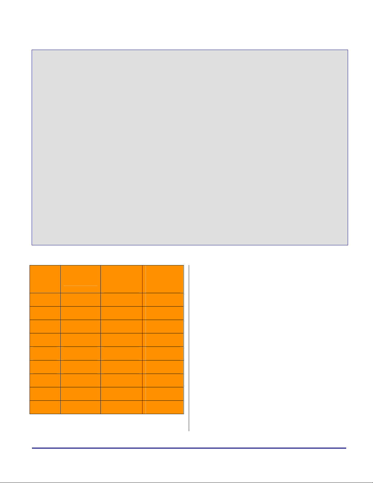
over the place. The solution lies in re-arranging a
stage’s output to ensure that the next stage’s
reads are sequential. The structure of the
algorithm implementation is shown in Figure 2.
Writing Efficient Floating-Point FFTs for ADSP-TS201 TigerSHARC® Processors (EE-218) Page 3 of 16
Page 4
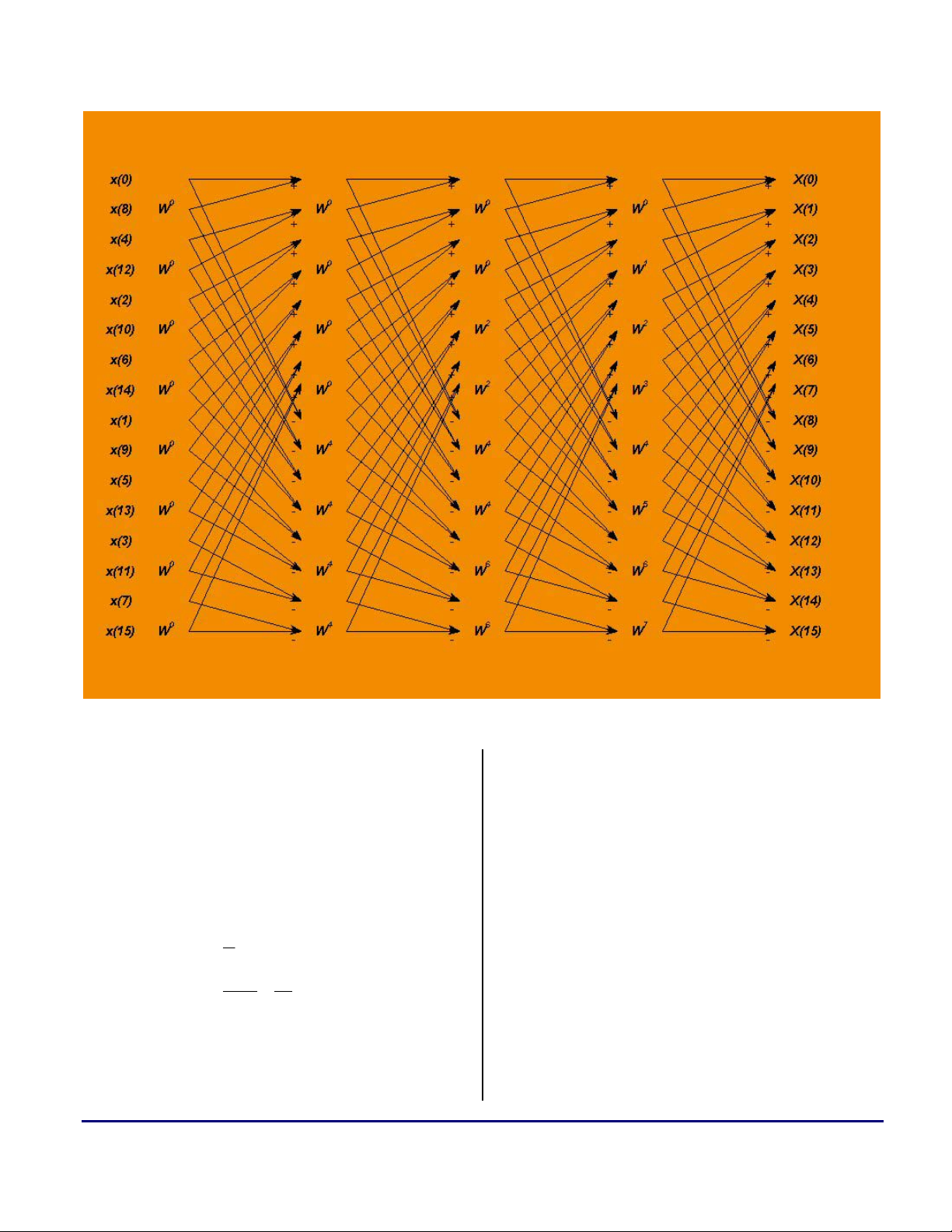
Figure 2. Reorganized Structure of the 16-Point FFT
It is simple enough to trace this diagram by hand
to see that it is simply a re-ordering of the
diagram in Figure 1. Amazingly enough, the final
output is in correct order. This can be easily
proven for general N = 2
in the FFT. Note that the re-ordering is given by
the following formula:
n
⎧
⎪
()
Thus, if n is even, it is shifted right and if n is
odd, it is shifted right and its most significant bit
is set. This is, of course, equivalent to the
Writing Efficient Floating-Point FFTs for ADSP-TS201 TigerSHARC® Processors (EE-218) Page 4 of 16
2
=
nf
⎨
⎪
⎩
k
= the number of points
even is if ,
n
−
1
Nn
+
22
odd is if ,
n
operation of right 1-bit rotation, which after
steps returns the original n back.
( )
NK2log=
Thus, the output after K stages is in correct order
again.
Great! We have our new structure. It has
sequential reads and we are lucky enough that
the output is in the correct order. This should be
much more efficient. Right? Let’s write the code
for it! Well, before we spend a lot of time writing
the code, we should ensure that all of the DSP
operations that we are about to do actually fit
into our processor architecture efficiently. There
may be no reason to optimize data movements if
the underlying math suffers.
Page 5
a
The first obvious point to notice is that this
structure cannot be done in-place due to its reordering. The stages will have to ping-pong their
input/output buffers. This should not be a
problem. The ADSP-TS201 processor has a lot
of memory on board, but should memory
optimization be required (and input does not
have to be preserved), we can use the input as
one of the two ping-pong buffers.
Next, we note that a traditional FFT combines
butterflies that share twiddles into the same
group to save twiddle fetch cycles. Amazingly,
the twiddles of the structure in Figure 2 line up
linearly – one group at a time. We are lucky
again!
Now, what would a butterfly of this new
structure consist of? Table 2 lists the operations
necessary to perform a single complex butterfly.
Since the ADSP-TS201 is a SIMD processor
(i.e., it can double all the computes), we will
write the steps outlined in Listing 1 in SIMD
fashion, so that two adjacent butterflies are
computed in parallel, one in the X-Compute
block and the other one in the Y-Compute block.
Let us analyze the DSP operations in more detail.
F1, F2, K2 and F4 fetch a total of four 32-bit
words, which on ADSP-TS201 can be done in a
single quad fetch into X-Compute block
registers. To be able to supply SIMD machine
with data, we would also have to perform a
second butterfly quad fetch into the Y-Compute
block registers. Then, M1, M2, M3, M4, A1, and
A2 will perform SIMD operations for both
butterflies.
The ADSP-TS201 supports a single add/subtract
instruction, so A3 and A4 can be combined into a
single operation (which is, of course, performed
SIMD on both butterflies at once) and similarly
A5 and A6 can be combined, as well.
Mnemonic Operation
F1
F2 Fetch Imag(Input1) of the Butterfly
K2 Fetch Real(Input2) of the Butterfly
F4 Fetch Imag(Input2) of the Butterfly
M1 K2 * Real(twiddle)
M2 F4 * Imag(twiddle)
M3 K2 * Imag(twiddle)
M4 F4 * Real(twiddle)
A1 M1–M2 = Real(Input2*twiddle)
A2 M3+M4 = Imag(Input2*twiddle)
A3 F1 + A1 = Real(Output1)
A4 F1 - A1 = Real(Output2)
A5 F2 + A2 = Imag(Output1)
A6 F2 – A2 = Imag(Output2)
S1 Store(Real(Output1))
S2 Store(Imag(Output1))
S3 Store(Real(Output2))
S4 Store(Imag(Output2))
Table 2. Single Butterfly Done Linearly – Logical
Implementation
Fetch Real(Input1) of the Butterfly
Now we run into a problem: S1, S2, S3 and S4
cannot be performed in the same cycle, since S3
and S4 are destined to another place in memory
due to our output re-ordering. Instead, we can
store S1 and S2 for
both butterflies in one cycle
(lucky again – these are adjacent!) and S3 and S4
for
both butterflies in the next cycle. So far, so
good – the new set of operations is summarized
in Table 3.
Writing Efficient Floating-Point FFTs for ADSP-TS201 TigerSHARC® Processors (EE-218) Page 5 of 16
Page 6

a
Mnemonic Operation
F1 Fetch Input1,2 of the Butterfly1
F2 Fetch Input1,2 of the Butterfly2
M1 Real(Input2) * Real(twiddle)
M2 Imag(Input2) * Imag(twiddle)
M3 Real(Input2) * Imag(twiddle)
M4 Imag(Input2) * Real(twiddle)
A1 M1–M2 = Real(Input2*twiddle)
A2 M3+M4 = Imag(Input2*twiddle)
A3 Real(Input1) +/- A1 = Real(Output1,2)
A4 Imag(Input1) +/- A2 = Imag(Output1)
S1 Store(Output1, both Butterflies)
S2 Store(Output2, both Butterflies)
Table 3. Single Butterfly Done Linearly – Actual
ADSP-TS20x Implementation
Each operation in Table 3 is a single-cycle
operation on ADSP-TS201 processor. There is a
total of 2 fetches, 4 multiplies, 4 ALU, and 2
store instructions. Since the ADSP-TS201 allows
fetches/stores to be paralleled with multiplies and
ALUs in a single cycle, loop unrolling,
pipelining, and paralleling should yield a 4-cycle
execution of these two SIMD butterflies (and we
are still efficient in the memory usage!). At this
point, we can now be reasonably certain that the
above will yield efficient code and we can start
developing it. However, careful observation at
this point can help us optimize this structure even
further. Note that we are only using a total of 4
fetches and stores from a single memory block,
say, by using JALU pointer registers. In parallel
we can do 3 more fetches/stores/KALU
operations without losing any cycles (actually,
we can do 4 of them, but we do need one
reserved place in one of the instructions for a
loop jump back).
Thus, the old rule of fetching twiddles only once
per group of butterflies that shares them is no
longer necessary – the twiddle fetches come free!
And, since the structure of the arrows of Figure 2
is identical at every stage, we may be able to
reduce the FFT from the usual three nested loops
to only two, provided that we can find a way to
correctly fetch the twiddles at each stage
(twiddles are the only thing that distinguishes the
stages of Figure 2). Figure 2 shows how the
twiddles must be fetched at each stage: 1
– all are W
N/4
W
. 3rd Stage – one quarter are W0, the next
quarter are W
the last quarter are W
0
. 2nd Stage – half are W0, next half are
N/8
, the next quarter are W
3N/8
. And so on… If we
st
Stage
2N/8
, and
keep a virtual twiddle pointer offset, increment it
to the next sequential twiddle every butterfly, but
AND it with a mask before actually using it in
the twiddle fetch, we achieve precisely this order
of twiddle fetch. Moreover, this rule is the same
for every stage, except that the mask at every
stage must be shifted down by one bit (i.e., each
stage requires twice as fine a resolution of the
twiddles as the previous stage). Here, our unused
KALU operations come in very handy. To
implement this twiddle fetch, we need to
increment the virtual offset, mask it and do a
twiddle fetch every butterfly… Oh, no! We are in
SIMD (i.e. we are doing two butterflies together)
and we do not have the 6 available instruction
slots for this! But luck saves us again. We can
easily notice that all stages except the last share
the twiddles between the SIMD pair of
butterflies – so, for these stages, we need only to
do the twiddle fetch once per SIMD pair of the
butterflies! And the three cycles are precisely
what we have to do this. Unfortunately, in the
last stage, every butterfly has its own unique
twiddle; but in the last stage, we do not have to
mask – just step the pointer to the next twiddle
every time! It will have to be written separately,
but it will optimize completely as well. Table 4
summarizes the latest structure’s steps. Three
Writing Efficient Floating-Point FFTs for ADSP-TS201 TigerSHARC® Processors (EE-218) Page 6 of 16
Page 7

a
new KALU operations (K1, K2 and K3) have
been added to Table 3. Time to write the code?
Well, no – let us figure out how to pipeline it
first.
Mnemonic Operation
K1 Virtual Pointer Offset Mask
K2 Twiddles Fetch
K3 Virtual Pointer Offset Increment
F1 Fetch Input1,2 of the Butterfly1
F2 Fetch Input1,2 of the Butterfly2
M1 Real(Input2) * Real(twiddle)
M2 Imag(Input2) * Imag(twiddle)
M3 Real(Input2) * Imag(twiddle)
M4 Imag(Input2) * Real(twiddle)
K2 -> M1, M2, M3, M4
F1, F2 -> M1, M2, M3, M4, A3, A4
M1, M2 -> A1
M3, M4 -> A2
A1, A2 -> A3, A4
This means that if the operation at the start of the
arrow is immediately followed by the operation
at the end of that arrow, the result will be correct,
but code execution will produce a stall. Thus, to
fully optimize the code, operations at the ends of
arrows with stalls must be kept more than one
instruction line apart.
A1 M1–M2 = Real(Input2*twiddle)
A2 M3+M4 = Imag(Input2*twiddle)
A3 Real(Input1) +/- A1 = Real(Output1,2)
A4 Imag(Input1) +/- A2 = Imag(Output1)
S1 Store(Output1, both Butterflies)
S2 Store(Output2, both Butterflies)
Table 4. Single Butterfly Done Linearly – Modified
ADSP-TS20x Implementation
Pipelining of the Algorithm
Figure 3 shows the algorithm’s operations from
Table 4 with arrows showing the dependencies.
The arrows of the dependencies indicate that the
result of the operation at the start of the arrow is
used by the operation at the end of that arrow
and, thus, must be completed first to ensure
correct data. Some arrows have a stall associated
with them, specifically:
Figure 3. Reorganized Structure’s Dependencies
A quick observation of the dependencies in
Figure 3 is sufficient to analyze the level of
pipelining and the number of compute block
registers needed to do it.
Writing Efficient Floating-Point FFTs for ADSP-TS201 TigerSHARC® Processors (EE-218) Page 7 of 16
Page 8

a
State
K1 K2 1 0
K2 M1,M2,M3,M4 5 4*([5/4]+1)=8
K3 K1 1 0
F1
F2
M1 A1 2 2([2/4]+1)=2
M2 A1 2 2([2/4]+1)=2
M3 A2 2 2([2/4]+1)=2
M4 A2 2 2([2/4]+1)=2
Dependency
To States
M1,M2,M3,M4,
A1,A2
M1,M2,M3,M4,
A1,A2
Max
Dep
Cycles
10 4*([10/4]+1)=16
10 4*([10/4]+1)=16
Compute Block
Registers
Needed
many output registers as
A2 since A3 and A4 are add/subtracts.
M1, M2, M3, M4, A1 and
The resulting requirement to fully pipeline this
code is 60 compute block registers, out of 64
total – just barely made it!
Cycle/
Operation
1 F1 K1 M4-- A3---
2 F2 K2 M2- A4---
3 S1--- M3- A2--
4 S2--- K3 M1 A1-
5 F1+ K1+ M4- A3--
6 F2+ K2+ M2 A4--
7 S1-- M3 A2-
JALU KALU MAC ALU
A1 A3,A4 2 2([2/4]+1)=2
A2 A3,A4 2 2([2/4]+1)=2
A3 S1,S2 1 4([1/4]+1)=4
A4 S1,S2 1 4([1/4]+1)=4
S1 none 0 0
S2 none 0 0
Table 5. Number of Compute Block Registers
Required to Pipeline the Butterflies
Total Regs
60
Full pipelining, as mentioned earlier, would give
a 4-cycle SIMD pair of butterflies. Thus,
Pipelined_CB_Registers_Per_State_Output =
Unpipelined_CB_Registers_Per_State_Output *
([Maximum_Dependency_Cycles/4]+1)
Here, [x] denotes the integer part of the number
x. We can therefore determine the number of
compute block registers needed, as shown in
Table 5. Note that
A3 and A4 require twice as
8 S2-- K3+ M1+ A1
9 F1++ K1++ M4 A3-
10 F2++ K2++ M2+ A4-
11 S1- M3+ A2
12 S2- K3++ M1++ A1+
13 F1+++ K1+++ M4+ A3
14 F2+++ K2+++ M2++ A4
15 S1 M3++ A2+
16 S2 K3+++ M1+++ A1++
Table 6. Pipelined Butterflies
We pipeline this fully symbolically, using the
mnemonics of Table 4 and Figure 3. The
pipelining is shown in Table 6, in which “+” in
the operation indicates the operation that
corresponds to the next set of the butterflies and
“-” corresponds to the operation in the previous
set of the butterflies.
Writing Efficient Floating-Point FFTs for ADSP-TS201 TigerSHARC® Processors (EE-218) Page 8 of 16
Page 9

a
All instructions are paralleled, there are no stalls,
and there is a place to put the jump to the top of
the loop (actually, four places, but this is only
because the pipeline is 4 pairs of butterflies deep,
each iteration of the loop in Table 6 will actually
do 4 pairs of butterflies).
The Code
Now, writing the code is trivial. The ADSPTS201 is so flexible that it takes all the challenge
right out of it. Just follow the pipeline of Table 6
and the code is done. The resulting code for the
stages other than last is shown in Listing 2.
Outside of this inner loop is a stage loop that
ping-pongs input/output buffers and shifts the
twiddle modifier mask. Pretty simple!
Additional optimization is done by breaking the
first two stages away from the main of the code
and doing them separately – they do not really
require a complex multiply and can be done
faster. Also, bit-reversal is incorporated into the
first two stages, as well. Now, for the bottom line
– how much did the cycle count improve? In
Table 7 we repeat Table 1 with additional
columns for the benchmarks for the new
algorithm. The cycle count for the larger-thancache FFTs improved by a factor greater than 3!
Moreover, the cycle count for FFTs that fit into
the cache is better than it was on the original
ADSP-TS101 processor, which had no cache or
memory latency issues of any kind. The reason
for this is that the new architecture allows the
code to be written in two nested loops instead of
three and, thus, has significantly less overhead.
This code, ported to the ADSP-TS101, improves
its benchmarks, too – as shown in Table 7.
.align_code 4;
_BflyLoop:
q[j2+=4]=r27:26; k5=k5+k9; fr6=r30*r12; fr16=r6-r7;; // S2----,K3-, M1-, A1--
yr3:0=q[j0+=4]; k3=k5 and k4; fr15=r23*r4; fr24=r8+r18, fr26=r8-r18;; // F1, K1, M4--, A3-- xr3:0=q[j0+=4]; r5:4=l[k7+k3]; fr7=r31*r13; fr25=r9+r19, fr27=r9-r19;; // F2, K2, M2-, A4-- q[j1+=4]=r25:24; fr14=r30*r13; fr17=r14+r15;; // S1---, M3-, A2- q[j2+=4]=r27:26; k5=k5+k9; fr6=r2*r4; fr18=r6-r7;; // S2---, K3, M1, A1-
yr11:8=q[j0+=4]; k3=k5 and k4; fr15=r31*r12; fr24=r20+r16, fr26=r20-r16;; // F1+, K1+, M4-, A3- xr11:8=q[j0+=4]; r13:12=l[k7+k3]; fr7=r3*r5; fr25=r21+r17, fr27=r21-r17;; // F2+, K2+, M2, A4- q[j1+=4]=r25:24; fr14=r2*r5; fr19=r14+r15;; // S1--, M3, A2 q[j2+=4]=r27:26; k5=k5+k9; fr6=r10*r12; fr16=r6-r7;; // S2--, K3+, M1+, A1
yr23:20=q[j0+=4]; k3=k5 and k4; fr15=r3*r4; fr24=r28+r18, fr26=r28-r18;; // F1++, K1++, M4, A3 xr23:20=q[j0+=4]; r5:4=l[k7+k3]; fr7=r11*r13; fr25=r29+r19, fr27=r29-r19;; // F2++, K2++, M2+, A4 q[j1+=4]=r25:24; fr14=r10*r13; fr17=r14+r15;; // S1-, M3+, A2
q[j2+=4]=r27:26; k5=k5+k9; fr6=r22*r4; fr18=r6-r7;; // S2-, K3++, M1++, A1+
yr31:28=q[j0+=4]; k3=k5 and k4; fr15=r11*r12; fr24=r0+r16, fr26=r0-r16;; // F1+++, K1+++, M4+, A3
xr31:28=q[j0+=4]; r13:12=l[k7+k3]; fr7=r23*r5; fr25=r1+r17, fr27=r1-r17;; // F2+++, K2+++, M2++, A4
.align_code 4;
if NLC0E, jump _BflyLoop;
q[j1+=4]=r25:24; fr14=r22*r5; fr19=r14+r15;; // S1, M3++, A2+
Listing 2. fft32.asm - fragment
Writing Efficient Floating-Point FFTs for ADSP-TS201 TigerSHARC® Processors (EE-218) Page 9 of 16
Page 10

a
ADSP-TS101
N
256 2172 1958 2641 2402 2218 1963
512 4582 4276 5533 5192 4649 4283
1024 9872 9410 12170 11662 9992 9419
2048 21338 20688 26610 25316 22173 20699
4096 46244 45278 197272 69924 NA NA
8192 99886 98540 444628 147628 NA NA
16384 215224 213243 987730 313292 NA NA
32768 NA NA 2133220 662614 NA NA
65536 NA NA 4720010 1397544 NA NA
Table 7. Core Clock Cycles for N-point Complex FFT, New versus Old Structure
Old structure
Usage Rules
The C-callable complex FFT routine is called as
FFT32( &(input), &(ping_pong_buffer1),
&(ping_pong_buffer2), &(output), N, F);
where
input -> FFT input buffer,
output -> FFT output buffer,
ping_pong_bufferx are the ping pong buffers,
N=Number of complex points,
ADSP-TS101
New structure
ADSP-TS201
Old structure-
Input not in
cache
ADSP-TS201
New structure-
Input not in
cache
ADSP-TS201
Old structure-
Input in cache
ADSP-TS201
New structureInput in cache
same as input if input does not need to be
preserved. Also, if Log
(N) is even, output can be
2
made the same as ping_pong_buffer2 and if
Log
(N) is odd, output can be made the same as
2
ping_pong_buffer1. Below are two examples of
the routine usage with minimal use of memory:
FFT32( &(input), &( input),
&( output), &(output), 1024, 1);
FFT32( &(input), &(input),
&( ping_pong_buffer2), &( input), 2048, 1);
To eliminate memory block access conflicts,
input must reside in a different memory block
F=0 if FFT is real and 1 if FFT is complex.
As mentioned earlier, due to data re-ordering,
stages cannot be done in-place and have to pingpong. Thus, ping_pong_buffer1 and
ping_pong_buffer2 have to be two distinct
buffers. However, depending on the routine’s
user requirements, some memory optimization is
possible. Ping_pong_buffer1 can be made the
than ping_pong_buffer2 and twiddle factors must
reside in a different memory block than the pingpong buffers. Of course, all code must reside in a
block that is different from all the data buffers, as
well. Ping-pong buffers can share a memory
block, however – there is no instruction that
accesses both ping-pong buffers in the same
cycle.
Writing Efficient Floating-Point FFTs for ADSP-TS201 TigerSHARC® Processors (EE-218) Page 10 of 16
Page 11

Appendix
Complete Source Code of the Optimized FFT
/* fft32.asm
Prelim rev. October 19, 2003 - BL
Rev. 1.0 - added real inputs case - PM
This is assembly routine for the Complex radix-2 C-callable FFT on TigerSHARC
family of DSPs.
I. Description of Calling.
1. Inputs:
j4 -> input (ping-pong buffer 1)
j5 -> ping-pong buffer 1
j6 -> ping-pong buffer 2
j7 -> output
j27+0x18 -> N = Number of points
j27+0x19 -> REAL or COMPLEX
2. C-Calling Example:
fft32(&(input), &(ping_pong_buffer1), &(ping_pong_buffer2), &(output), N, COMPLEX);
3. Limitations:
a. All buffers must be aligned on memory boundary which is a multiple of 4.
b. N must be between 32 and MAX_FFT_SIZE.
c. If memory space savings are required and input does not have to be
preserved, ping_pong_buffer1 can be the same buffer as input.
d. If memory space savings are required, output can be the same buffer
as ping_pong_buffer2 if the number of FFT stages is even (i.e.
Log2(N) is even) or the same as ping_pong_buffer1 if the number of
FFT stages is odd (i.e. Log2(N) is odd).
4. MAX_FFT_SIZE can be selected via #define. Larger values allow for more choices
of N, but its twiddles will occupy more memory.
5. This C - callable function can process up to 64K blocks of data on TS201
(16K blocks on TS101) because C environment itself necessitates memory.
Therefore, if more input points are necessary, assembly language development
may become a must. On TS201, a block of memory is 128K words long, so
maximum N is 128K real points or 64K complex points. TS101 contains
only 2 blocks of data memory of 64K words and 4 buffers must be
accommodated. Therefore, maximum N is 32K real words or 16K complex words.
II. Description of the FFT algorithm.
1. The input data is treated as complex interleaved N-point.
2. Due to re-ordering, no stage can be done in-place.
3. The bit reversal and the first two stages are combined into
a single loop. This loop takes data from input and stores it
in the ping-pong buffer1.
4. Each subsequent stage ping-pongs the data between the two ping-pong
buffers. The last stage uses FFT output buffer for its output.
5. Although the FFT is designed to be called with any point size
N <= MAX_FFT_SIZE by subsampling the twiddle factors, for ADSP-TS20x
processors, the best cycle optimization is achieved when MAX_FFT_SIZE=N.
For ADSP-TS101 all choices of MAX_FFT_SIZE are equally optimal.
III. Description of the REAL FFT algorithm.
1. The input data is treated as complex interleaved N/2-point. The N/2 point complex
FFT will be computed first. Thus, N is halved, now number of points = N/2.
2. Details and source code of the N/2 point complex FFT are in II above.
3. Real re-combine:
Here the complex N/2-point FFT computed in the previous steps is recombined to
produce the N-point real FFT. If G is the complex FFT and F is the real FFT,
the formula for F is given by:
F(n) = 0.5*(G(n)+conj(G(N/2-n))-0.5*i*exp(-2*pi*i*n/N)*(G(n)-conj(G(N/2-n)).
From this the following can be derived:
conj(F(N/2-n)) = 0.5*(G(n)+conj(G(N/2-n))+0.5*i*exp(-2*pi*i*n/N)*(G(n)-conj(G(N/2-n)).
Thus, this can be computed in (n,N/2-n) pairs, as follows (dropping factor of 2):
G(n) ------------------------------->------------------------>--------> F(n)
\ +/ \ +/
\/ \/
/\ /\
conj / -\ exp(-2*pi*i*n)*i / -\ conj
G(N/2-n) -----> conj(G(N/2-n))------>------------------------>--------> F(N/2-n)
This is very efficient on the TigerSHARC architecture due to the add/subtract
instruction.
IV. For all additional details regarding this algorithm and code, see EE-218
a
Writing Efficient Floating-Point FFTs for ADSP-TS201 TigerSHARC® Processors (EE-218) Page 11 of 16
Page 12

application note, available from the ADI web site.
*/
//************************************ Includes **********************************
#include "FFTDef.h"
#include "defts201.h"
//************************* Externs *************************************
.extern _twiddles;
//********************************* FFT Routine *********************************
.section program;
.global _FFT32;
_FFT32:
//********************************** Prologue ***********************************
mENTER
mPUSHQ(xR31:28)
mPUSHQ(xR27:24)
mPUSHQ(yR31:28)
mPUSHQ(yR27:24)
//************************************ Setup *************************************
j17 = [j27 + 0x18];; //j17 = N
j11 = [j27 + 0x19];; // j11=COMPLEX or REAL, off the stack
comp(j11,COMPLEX);; // Complex or Real?
if jeq, jump _FFTStages1and2;;
j17=ashiftr j17;; // if Real, half N
//********************************************************************************
_FFTStages1and2:
j11 = j31 + j17;; // j11=N
xr3=j11; k7=k31+_twiddles;;
k1=j11; j8=lshiftr j11;; // k1=N, j8=N/2
j9=lshiftr j8; xr0=MAX_FFT_SIZE; xr3=LD0 r3;; // j9=N/4, compute the twiddle stride
k8=lshiftr k1; xr0=LD0 r0; xr1=j11;;
k8=lshiftr k8; xr1=LD0 r1; xr2=(31-3);; // k8=N/4, Compute Stages-3
k0=j4; k10=lshiftr k8; xr1=r1-r0; xr0=lshift r0 by -32;; // k0->input, xr1=bit difference between MAX and N
k10=lshiftr k10; xr0=bset r0 by r1; xr30=r2-r3;; // k10=N/16, xr30=Stages-3
k10=k10-1; xr0=lshift r0 by 2; LC1=xr30;; // k10=N/16-1, LC1=Stages-3
k9=xr0; k4=k31+(MAX_FFT_SIZE/4-1);;
k4=not k4; j10=lshiftr j9;; // initial twiddles pointer mask, j10=N/8
//****************** Bit Reverse and Stages 1 & 2 ******************************
k5=lshiftr k1;; // k5=N/2
j0=j31+j6; k6=k6-k6;; // j0->ping_pong_buffer2
j1=j0+j9; LC0=k10;; // j1->ping_pong_buffer2+N/4, LC0=N/16-1
j2=j1+j9; k1=k0+k5;; // j2->ping_pong_buffer2+N/2, k1->input+N/2
j3=j2+j9; k2=k1+k5;; // j3->ping_pong_buffer2+3N/4, k2->input+N
j12=j3+j9; k3=k2+k5;; // j12->ping_pong_buffer2+N, k3->input+3N/2
j13=j12+j9; k5=lshiftr k5;; // j13->ping_pong_buffer2+5N/4, k5=N/4
j14=j13+j9; r1:0=q[k0+k6];; // j14->ping_pong_buffer2+3N/2
j15=j14+j9; r3:2=q[k2+k6];; // j15->ping_pong_buffer2+7N/4
r5:4=q[k1+k6];;
r7:6=q[k3+k6];;
k6=k6+k5 (br); fr0=r0+r2, fr20=r0-r2;;
r9:8=q[k0+k6]; fr2=r1+r3, fr29=r1-r3;;
r11:10=q[k2+k6]; fr4=r4+r6, fr21=r4-r6;;
r13:12=q[k1+k6]; fr5=r5+r7, fr28=r5-r7;;
r15:14=q[k3+k6]; fr18=r8+r10, fr22=r8-r10;;
k6=k6+k5 (br); fr19=r9+r11, fr31=r9-r11;;
fr26=r12+r14, fr23=r12-r14;;
fr27=r13+r15, fr30=r13-r15;;
fr20=r20+r28, fr28=r20-r28;;
fr29=r29+r21, fr21=r29-r21;;
fr22=r22+r30, fr30=r22-r30;;
fr31=r31+r23, fr23=r31-r23;;
.align_code 4;
_Stages1and2Loop:
r1:0=q[k0+k6]; q[j2+=4]=yr23:20; fr16=r0+r4, fr24=r0-r4;;
r3:2=q[k2+k6]; q[j3+=4]=xr23:20; fr17=r2+r5, fr25=r2-r5;;
r5:4=q[k1+k6]; q[j14+=4]=yr31:28; fr18=r18+r26, fr26=r18-r26;;
r7:6=q[k3+k6]; q[j15+=4]=xr31:28; fr19=r19+r27, fr27=r19-r27;;
k6=k6+k5 (br); q[j0+=4]=yr19:16; fr0=r0+r2, fr20=r0-r2;;
r9:8=q[k0+k6]; q[j1+=4]=xr19:16; fr2=r1+r3, fr29=r1-r3;;
r11:10=q[k2+k6]; q[j12+=4]=yr27:24; fr4=r4+r6, fr21=r4-r6;;
r13:12=q[k1+k6]; q[j13+=4]=xr27:24; fr5=r5+r7, fr28=r5-r7;;
r15:14=q[k3+k6]; fr18=r8+r10, fr22=r8-r10;;
k6=k6+k5 (br); fr19=r9+r11, fr31=r9-r11;;
fr26=r12+r14, fr23=r12-r14;;
fr27=r13+r15, fr30=r13-r15;;
fr20=r20+r28, fr28=r20-r28;;
fr29=r29+r21, fr21=r29-r21;;
fr22=r22+r30, fr30=r22-r30;;
a
Writing Efficient Floating-Point FFTs for ADSP-TS201 TigerSHARC® Processors (EE-218) Page 12 of 16
Page 13

.align_code 4;
if NLC0E, jump _Stages1and2Loop;
fr31=r31+r23, fr23=r31-r23;;
q[j2+=4]=yr23:20; fr16=r0+r4, fr24=r0-r4;;
q[j3+=4]=xr23:20; fr17=r2+r5, fr25=r2-r5;;
q[j14+=4]=yr31:28; fr18=r18+r26, fr26=r18-r26;;
q[j15+=4]=xr31:28; fr19=r19+r27, fr27=r19-r27;;
q[j0+=4]=yr19:16;;
q[j1+=4]=xr19:16;;
q[j12+=4]=yr27:24;;
q[j13+=4]=xr27:24;;
//************************ Stages 3 to Log2(N)-1 *******************************
j0=j31+j6; k5=k31+0;;
.align_code 4;
_StageLoop:
yr3:0=q[j0+=4]; k3=k5 and k4;; // F1, K1
xr3:0=q[j0+=4]; r5:4=l[k7+k3];; // F2, K2
LC0=k10; k5=k5+k9;; // K3, M1
yr11:8=q[j0+=4]; k3=k5 and k4; fr6=r2*r4;; // F1+, K1+
xr11:8=q[j0+=4]; r13:12=l[k7+k3]; fr7=r3*r5;; // F2+, K2+, M2
fr14=r2*r5;; // M3
j1=j31+j5; k5=k5+k9; fr6=r10*r12; fr16=r6-r7;; // K3+, M1+, A1
yr23:20=q[j0+=4]; k3=k5 and k4; fr15=r3*r4;; // F1++, K1++, M4
xr23:20=q[j0+=4]; r5:4=l[k7+k3]; fr7=r11*r13;; // F2++, K2++, M2+
fr14=r10*r13; fr17=r14+r15;; // M3+, A2
j2=j1+j11; k5=k5+k9; fr6=r22*r4; fr18=r6-r7;; // K3++, M1++, A1+
yr31:28=q[j0+=4]; k3=k5 and k4; fr15=r11*r12; fr24=r0+r16, fr26=r0-r16;; // F1+++, K1+++, M4+, A3
xr31:28=q[j0+=4]; r13:12=l[k7+k3]; fr7=r23*r5; fr25=r1+r17, fr27=r1-r17;; // F2+++, K2+++, M2++, A4
q[j1+=4]=r25:24; fr14=r22*r5; fr19=r14+r15;; // S1, M3++, A2+
.align_code 4;
_BflyLoop:
q[j2+=4]=r27:26; k5=k5+k9; fr6=r30*r12; fr16=r6-r7;; // S2----,K3-, M1-, A1--
yr3:0=q[j0+=4]; k3=k5 and k4; fr15=r23*r4; fr24=r8+r18, fr26=r8-r18;; // F1, K1, M4--, A3-- xr3:0=q[j0+=4]; r5:4=l[k7+k3]; fr7=r31*r13; fr25=r9+r19, fr27=r9-r19;; // F2, K2, M2-, A4-- q[j1+=4]=r25:24; fr14=r30*r13; fr17=r14+r15;; // S1---, M3-, A2- q[j2+=4]=r27:26; k5=k5+k9; fr6=r2*r4; fr18=r6-r7;; // S2---, K3, M1, A1-
yr11:8=q[j0+=4]; k3=k5 and k4; fr15=r31*r12; fr24=r20+r16, fr26=r20-r16;; // F1+, K1+, M4-, A3- xr11:8=q[j0+=4]; r13:12=l[k7+k3]; fr7=r3*r5; fr25=r21+r17, fr27=r21-r17;; // F2+, K2+, M2, A4- q[j1+=4]=r25:24; fr14=r2*r5; fr19=r14+r15;; // S1--, M3, A2 q[j2+=4]=r27:26; k5=k5+k9; fr6=r10*r12; fr16=r6-r7;; // S2--, K3+, M1+, A1
yr23:20=q[j0+=4]; k3=k5 and k4; fr15=r3*r4; fr24=r28+r18, fr26=r28-r18;; // F1++, K1++, M4, A3 xr23:20=q[j0+=4]; r5:4=l[k7+k3]; fr7=r11*r13; fr25=r29+r19, fr27=r29-r19;; // F2++, K2++, M2+, A4 q[j1+=4]=r25:24; fr14=r10*r13; fr17=r14+r15;; // S1-, M3+, A2
q[j2+=4]=r27:26; k5=k5+k9; fr6=r22*r4; fr18=r6-r7;; // S2-, K3++, M1++, A1+
yr31:28=q[j0+=4]; k3=k5 and k4; fr15=r11*r12; fr24=r0+r16, fr26=r0-r16;; // F1+++, K1+++, M4+, A3
xr31:28=q[j0+=4]; r13:12=l[k7+k3]; fr7=r23*r5; fr25=r1+r17, fr27=r1-r17;; // F2+++, K2+++, M2++, A4
.align_code 4;
if NLC0E, jump _BflyLoop;
q[j1+=4]=r25:24; fr14=r22*r5; fr19=r14+r15;; // S1, M3++, A2+
q[j2+=4]=r27:26; fr6=r30*r12; fr16=r6-r7;; // S2----, M1-, A1--
j0=j31+j5; fr15=r23*r4; fr24=r8+r18, fr26=r8-r18;; // M4--, A3-- // swap ping-pong pointers
j5=j31+j6; fr7=r31*r13; fr25=r9+r19, fr27=r9-r19;; // M2-, A4-- q[j1+=4]=r25:24; fr14=r30*r13; fr17=r14+r15;; // S1---, M3-, A2- q[j2+=4]=r27:26; fr18=r6-r7;; // S2---, A1-
j6=j31+j0; fr15=r31*r12; fr24=r20+r16, fr26=r20-r16;; // M4-, A3- fr25=r21+r17, fr27=r21-r17;; // A4- q[j1+=4]=r25:24; fr19=r14+r15;; // S1--, A2 q[j2+=4]=r27:26; fr24=r28+r18, fr22=r28-r18;; // S2-- A3-
j0=j31+j6; fr25=r29+r19, fr23=r29-r19;; // A4 q[j1+=4]=r25:24; k5=k31+0;; // S1.align_code 4;
if NLC1E, jump _StageLoop;
q[j2+=4]=r23:22; k4=ashiftr k4;; // S2-, shift the mask
//******************************* Last stage *********************************
k9 = ashiftr k9;;//in this manner any MAX_FFT_SIZE can be used
yr3:0=q[j0+=4]; yr5:4 = l[k7+=k9];; // F1,
xr3:0=q[j0+=4]; xr5:4=l[k7+=k9];; // F2, K2
j1=j31+j7; fr6=r2*r4; LC0=k10;; // M1
yr11:8=q[j0+=4]; yr13:12=l[k7+=k9];; // F1+
xr11:8=q[j0+=4]; xr13:12=l[k7+=k9]; fr7=r3*r5;; // F2+, K2+, M2
j2=j1+j11; fr14=r2*r5;; // M3
fr6=r10*r12; fr16=r6-r7;; // M1+, A1
yr23:20=q[j0+=4]; yr5:4=l[k7+=k9]; fr15=r3*r4;; // F1++, M4
xr23:20=q[j0+=4]; xr5:4=l[k7+=k9]; fr7=r11*r13;; // F2++, K2++, M2+
fr14=r10*r13; fr17=r14+r15;; // M3+, A2
fr6=r22*r4; fr18=r6-r7;; // M1++, A1+
a
Writing Efficient Floating-Point FFTs for ADSP-TS201 TigerSHARC® Processors (EE-218) Page 13 of 16
Page 14

yr31:28=q[j0+=4]; yr13:12=l[k7+=k9];fr15=r11*r12; fr24=r0+r16, fr26=r0-r16;; // F1+++, M4+, A3
xr31:28=q[j0+=4]; xr13:12=l[k7+=k9]; fr7=r23*r5; fr25=r1+r17, fr27=r1-r17;; // F2+++, K2+++, M2++, A4
q[j1+=4]=r25:24; fr14=r22*r5; fr19=r14+r15;; // S1, M3++, A2+
.align_code 4;
_BflyLastLoop:
q[j2+=4]=r27:26; fr6=r30*r12; fr16=r6-r7;; // S2----, M1-, A1--
yr3:0=q[j0+=4]; yr5:4=l[k7+=k9]; fr15=r23*r4; fr24=r8+r18, fr26=r8-r18;; // F1, M4--, A3-- xr3:0=q[j0+=4]; xr5:4=l[k7+=k9]; fr7=r31*r13; fr25=r9+r19, fr27=r9-r19;; // F2, K2, M2-, A4-- q[j1+=4]=r25:24; fr14=r30*r13; fr17=r14+r15;; // S1---, M3-, A2- q[j2+=4]=r27:26; fr6=r2*r4; fr18=r6-r7;; // S2---, M1, A1-
yr11:8=q[j0+=4]; yr13:12=l[k7+=k9];fr15=r31*r12; fr24=r20+r16, fr26=r20-r16;; // F1+, M4-, A3- xr11:8=q[j0+=4]; xr13:12=l[k7+=k9];fr7=r3*r5; fr25=r21+r17, fr27=r21-r17;; // F2+, K2+, M2, A4- q[j1+=4]=r25:24; fr14=r2*r5; fr19=r14+r15;; // S1--, M3, A2 q[j2+=4]=r27:26; fr6=r10*r12; fr16=r6-r7;; // S2--, M1+, A1
yr23:20=q[j0+=4]; yr5:4=l[k7+=k9]; fr15=r3*r4; fr24=r28+r18, fr26=r28-r18;; // F1++, M4, A3 xr23:20=q[j0+=4]; xr5:4=l[k7+=k9]; fr7=r11*r13; fr25=r29+r19, fr27=r29-r19;; // F2++, K2++, M2+, A4 q[j1+=4]=r25:24; fr14=r10*r13; fr17=r14+r15;; // S1-, M3+, A2
q[j2+=4]=r27:26; fr6=r22*r4; fr18=r6-r7;; // S2-, M1++, A1+
yr31:28=q[j0+=4];yr13:12=l[k7+=k9]; fr15=r11*r12; fr24=r0+r16, fr26=r0-r16;; // F1+++, M4+, A3
xr31:28=q[j0+=4];xr13:12=l[k7+=k9]; fr7=r23*r5; fr25=r1+r17, fr27=r1-r17;; // F2+++, K2+++, M2++, A4
.align_code 4;
if NLC0E, jump _BflyLastLoop;
q[j1+=4]=r25:24; fr14=r22*r5; fr19=r14+r15;; // S1, M3++, A2+
q[j2+=4]=r27:26; fr6=r30*r12; fr16=r6-r7;; // S2----, M1-, A1- fr15=r23*r4; fr24=r8+r18, fr26=r8-r18;; // M4--, A3-- fr7=r31*r13; fr25=r9+r19, fr27=r9-r19;; // M2-, A4-- q[j1+=4]=r25:24; fr14=r30*r13; fr17=r14+r15;; // S1---, M3-, A2- q[j2+=4]=r27:26; fr18=r6-r7;; // S2---, A1 fr15=r31*r12; fr24=r20+r16, fr26=r20-r16;; // M4-, A3- fr25=r21+r17, fr27=r21-r17;; // A4- q[j1+=4]=r25:24; fr19=r14+r15;; // S1--, A2 q[j2+=4]=r27:26;; // S2- fr24=r28+r18, fr26=r28-r18;; // A3 fr25=r29+r19, fr27=r29-r19;; // A4 q[j1+=4]=r25:24;; // S1 q[j2+=4]=r27:26;; // S2 j11=[j27+0x19];; // j11=COMPLEX or REAL, off the stack
comp(j11,COMPLEX);; // Complex or Real?
.align_code 4;
if jeq, jump _FFTEpilogue;; // If Complex, done
//******************************* Real re-combine ********************************
//j17=N/2, j7=output
k8=k31+_twiddles; j0=j31+j7;; // k8->twiddles, j0->internal buffer
k9=ashiftr k9; j10=j31+j7;; // k9=twiddle stride, j10->internal buffer
j14=j17+j17;; // j14=N (N/2 complex values)
j14=j14-4;; // j14=N-4 real=N/2-2 complex
j1=j0+j14;; // j1->internal buffer+(N/2-2)
j14=j10+j14;; // j14->internal buffer+(N/2-2)
j29 = ashiftr j17;; // j29=N/4
k15=k31+MAX_FFT_SIZE/4; j30=ashiftr j29;; // k15=N/4*twiddle_stride, j30=N/8
j30 = ashiftr j30;; // N/16
k8=k8+k9; r0=l[j7+j17];; // k8->twiddles+1, get G(N/4)
j0=j0+2; k12=k8+k15;; // j0->internal buffer+1, k12->twiddles+N/8+1
LC0=j30; fr0=r0+r0; j2=j0+j29;; // LC0=N/16, compute F(N/4)=2*conj(G(N/4)),
// j2->internal buffer+1+N/8
j3=j1-j29;; // j3->internal buffer+3N/8-2
xfr0=-r0; j10=j10+2; k10=yr0;; // j10->internal buffer+1, k10=Im(F(N/4))
j12=j10+j29;; // j12->internal buffer+N/8+1
if LC0E; j13=j14-j29; k11=xr0;; // LC0=N/16-1, j13->internal buffer+3N/8-2, k11=Re(F(N/4))
yr3:0=DAB q[j0+=4];; // Prime the DAB
xr3:0=DAB q[j2+=4];; // Prime the DAB
yr3:0=DAB q[j0+=4];; // yr0=Re(G(n)), yr1=Im(G(n)), yr2=Re(G(n+1)), yr3=Im(G(n+1))
xr3:0=DAB q[j2+=4];; // xr0=Re(G(n+N/8)), xr1=Im(G(n+N/8))
// xr2=Re(G(n+1+N/8)), xr3=Im(G(n+1+N/8))
yr7:4=q[j1+=-4]; xr9:8=l[k12+=k9];; // yr4=Re(G(N/2-(n+1))), yr5=Im(G(N/2-(n+1)))
// yr6=Re(G(N/2-n)), yr7=Im(G(N/2-n))
// twiddles(n+N/8) - want to mult by sin(x)-icos(x)
xr7:4=q[j3+=-4]; xr11:10=l[k12+=k9];; // xr4=Re(G(N/2-(n+1+N/8))), xr5=Im(G(N/2-(n+1+N/8)))
// xr6=Re(G(N/2-(n+N/8))), xr7=Im(G(N/2-(n+N/8)))
// twiddles(n+1+N/8)
if LC0E; fr16=r0+r6, fr20=r0-r6; yr9:8=l[k8+=k9];; // LC0=N/16-2, r16=Re(G(n)+conj(G(N/2-n))),
// r20=Re(G(n)-conj(G(N/2-n)))
// twiddles(n)
fr18=r2+r4, fr22=r2-r4; yr11:10=l[k8+=k9];; // r18=Re(G(n+1)+conj(G(N/2-(n+1)))),
// r22=Re(G(n+1)-conj(G(N/2-(n+1))))
// twiddles(n+1)
fr24=r20*r9; fr21=r1+r7, fr17=r1-r7;; // r24=s(n)*Re(G(n)-conj(G(N/2-n)))
// r17=Im(G(n)+conj(G(N/2-n))), r21=Im(G(n)-conj(G(N/2-n)))
fr26=r22*r11; fr23=r3+r5, fr19=r3-r5; xr3:0=DAB q[j2+=4];; // r26=s(n+1)*Re(G(n+1)-conj(G(N/2-(n+1))))
// r19=Im(G(n+1)+conj(G(N/2-(n+1)))),
// r23=Im(G(n+1)-conj(G(N/2-(n+1))))
// xr3:0=next G(n+2+N/8), G(n+3+N/8)
fr25=r21*r8; yr3:0=DAB q[j0+=4];; // r25=c(n)*Im(G(n)-conj(G(N/2-n))),
// yr3:0=next G(n+2), G(n+3)
fr27=r23*r10;; // r27=c(n+1)*Im(G(n+1)-conj(G(N/2-(n+1))))
fr24=r24+r25; fr25=r21*r9; yr7:4=q[j1+=-4];; // r24=Re(-i*exp(2*pi*i*n)(G(n)-conj(G(N/2-n))))
// r13=s(n)*Im(G(n)-conj(G(N/2-n)))
// yr7:4=next G(N/2-(n+2)), G(N/2-(n+3))
fr26=r26+r27; fr27=r23*r11; xr7:4=q[j3+=-4];; // r26=Re(-i*exp(2*pi*i*(n+1))(G(n+1)-conj(G(N/2-(n+1)))))
a
Writing Efficient Floating-Point FFTs for ADSP-TS201 TigerSHARC® Processors (EE-218) Page 14 of 16
Page 15

// r27=s(n+1)*Im(G(n+1)-conj(G(N/2-(n+1))))
// xr7:4=next G(N/2-(n+2+N/8)), G(N/2-(n+3+N/8))
fr13=r20*r8; fr12=r16+r24, fr30=r16-r24;; // r13=c(n)*Re(G(n)-conj(G(N/2-n))),
// r12=Re(F(n)), r30=Re(F(N/2-n))
fr15=r22*r10; fr14=r18+r26, fr28=r18-r26;; // r15=c(n+1)*Re(G(n+1)-conj(G(N/2-(n+1))))
// r14=Re(F(n+1)), r28=Re(F(N/2-(n+1)))
fr13=r25-r13; xr9:8=l[k12+=k9];; // r13=Im(-i*exp(2*pi*i*x)(G(n)-conj(G(N/2-n)))),
// next twiddles(n+2+N/8)
fr15=r27-r15; xr11:10=l[k12+=k9];; // r15=Im(-i*exp(2*pi*i*x)(G(n+1)-conj(G(N/2-(n+1)))))
// next twiddles(n+3+N/8)
.align_code 4;
_combine_stage:
fr16=r0+r6, fr20=r0-r6; yr9:8=l[k8+=k9];; // r16=Re(G(n+2)+conj(G(N/2-(n+2)))),
// r20=Re(G(n+2)-conj(G(N/2-(n+2))))
// next twiddles(n+2)
fr18=r2+r4, fr22=r2-r4; yr11:10=l[k8+=k9];; // r18=Re(G(n+3)+conj(G(N/2-(n+3)))),
// r22=Re(G(n+3)-conj(G(N/2-(n+3))))
// next twiddles(n+3)
fr13=r13+r17, fr31=r13-r17;; // r13=Im(F(n)), r31=Im(F(N/2-n))
fr15=r15+r19, fr29=r15-r19; l[j12+=2]=xr13:12;; // r15=Im(F(n+1)), r29=Im(F(N/2-(n+1))), store F(n+N/8)
fr24=r20*r9; fr21=r1+r7, fr17=r1-r7; q[j14+=-4]=yr31:28;; // r24=s(n+2)*Re(G(n+2)-conj(G(N/2-(n+2))))
// r21=Im(G(n+2)+conj(G(N/2-(n+2)))),
// r17=Im(G(n+2)-conj(G(N/2-(n+2))))
// store F(N/2-n), F(N/2-(n+1))
fr26=r22*r11; fr23=r3+r5, fr19=r3-r5; xr3:0=DAB q[j2+=4];; // r26=s(n+3)*Re(G(n+3)-conj(G(N/2-(n+3))))
// r23=Im(G(n+3)+conj(G(N/2-(n+3)))),
// r19=Im(G(n+3)-conj(G(N/2-(n+3))))
// xr3:0=next G(n+4+N/8), G(n+5+N/8)
fr25=r21*r8; yr3:0=DAB q[j0+=4];; // r25=c(n+2)*Im(G(n+2)-conj(G(N/2-(n+2))))
// yr3:0=next G(n+4), G(n+5)
fr27=r23*r10; q[j13+=-4]=xr31:28;; // r27=c(n+3)*Im(G(n+3)-conj(G(N/2-(n+3))))
// store F(N/2-(n+N/8)), F(N/2-(n+1+N/8))
fr24=r24+r25; fr25=r21*r9; l[j10+=2]=yr13:12;; // r24=Re(-i*exp(2*pi*i*x)(G(n+2)-conj(G(N/2-(n+2)))))
// r25=s(n+2)*Im(G(n+2)-conj(G(N/2-(n+2)))), store F(n)
fr26=r26+r27; fr27=r23*r11; l[j10+=2]=yr15:14;; // r26=Re(-i*exp(2*pi*i*x)(G(n+3)-conj(G(N/2-(n+3)))))
// r27=s(n+3)*Im(G(n+3)-conj(G(N/2-(n+3)))), store F(n+1)
fr13=r20*r8; fr12=r16+r24, fr30=r16-r24; l[j12+=2]=xr15:14;; // r13=cos(n+2)*Re(G(n+2)-conj(G(N/2-(n+2))))
// r12=Re(F(n+2)), r30=Re(F(N/2-(n+2))), store F(n+1+N/8)
fr15=r22*r10; fr14=r18+r26, fr28=r18-r26; xr7:4=q[j3+=-4];; // r15=cos(n+3)*Re(G(n+3)-conj(G(N/2-(n+3))))
// r14=Re(F(n+3)), r28=Re(F(N/2-(n+3)))
// xr7:4=next G(N/2-(n+4+N/8)), G(N/2-(n+5+N/8))
fr13=r25-r13; xr9:8=l[k12+=k9]; yr7:4=q[j1+=-4];; // r13=Im(-i*exp(2*pi*i*x)(G(n+2)-conj(G(N/2-(n+2)))))
// next twiddles(n+4+N/8)
// yr7:4=next G(N/2-(n+4)), G(N/2-(n+5))
.align_code 4;
if NLC0E, jump _combine_stage(P); fr15=r27-r15; xr11:10=l[k12+=k9];;// r15=Im(-i*exp(2*pi*i*x)(G(n+3)-conj(G(N/2-(n+3)))))
// next twiddles(n+5+N/8)
fr16=r0+r6, fr20=r0-r6; yr9:8=l[k8+=k9];; // r16=Re(G(n+4)+conj(G(N/2-(n+4)))),
// r20=Re(G(n+4)-conj(G(N/2-(n+4))))
// next twiddles(n+4)
fr18=r2+r4, fr22=r2-r4; yr11:10=l[k8+=k9];; // r18=Re(G(n+5)+conj(G(N/2-(n+5)))),
// r22=Re(G(n+5)-conj(G(N/2-(n+5))))
// next twiddles(n+5)
fr13=r13+r17, fr31=r13-r17;; // r13=Im(F(n+2)), r31=Im(F(N/2-(n+2)))
fr15=r15+r19, fr29=r15-r19;; // r15=Im(F(n+3)), r29=Im(F(N/2-(n+3)))
fr24=r20*r9; fr21=r1+r7, fr17=r1-r7; yr1:0=l[j31+j7];; // r24=s(n+4)*Re(G(n+4)-conj(G(N/2-(n+4))))
// r21=Im(G(n+4)+conj(G(N/2-(n+4)))),
// r17=Im(G(n+4)-conj(G(N/2-(n+4))))
// yr0=Re(G(0)), yr1=Im(G(0))
fr26=r22*r11; fr23=r3+r5, fr19=r3-r5;; // r26=s(n+5)*Re(G(n+5)-conj(G(N/2-(n+5))))
// r23=Im(G(n+5)+conj(G(N/2-(n+5)))),
// r19=Im(G(n+5)-conj(G(N/2-(n+5))))
fr25=r21*r8;; // r25=cos(x)*Im(G(n)-conj(G(N/2-n)))
fr27=r23*r10; l[j12+=2]=xr13:12;; // r27=cos(x)*Im(G(n)-conj(G(N/2-n)))
// store F(n+2+N/8)
yfr0=r1+r0; yr1=lshift r1 by -32; q[j14+=-4]=yr31:28;; // yr0=Re(G(0))+Im(G(0)), yr1=0=Im(F(0))
// store F(N/2-(n+2)), F(N/2-(n+3))
yfr0=r0+r0; q[j13+=-4]=xr31:28;; // yr0=Re(F(0))
// store F(N/2-(n+2+N/8)), F(N/2-(n+3+N/8))
fr24=r24+r25; fr25=r21*r9; l[j10+=2]=yr13:12;; // r24=Re(-i*exp(2*pi*i*x)(G(n+4)-conj(G(N/2-(n+4)))))
// r25=s(n+4)*Im(G(n+4)-conj(G(N/2-(n+4)))), store F(n+2)
fr26=r26+r27; fr27=r23*r11; l[j10+=2]=yr15:14;; // r26=Re(-i*exp(2*pi*i*x)(G(n+5)-conj(G(N/2-(n+5)))))
// r27=s(n+5)*Im(G(n+5)-conj(G(N/2-(n+5)))), store F(n+3)
fr13=r20*r8; fr12=r16+r24, fr30=r16-r24; l[j12+=2]=xr15:14;; // r13=c(n+4)*Re(G(n+4)-conj(G(N/2-(n+4))))
// r12=Re(F(n+4)), r30=Re(F(N/2-(n+4))), store F(n+3+N/8)
fr15=r22*r10; fr14=r18+r26, fr28=r18-r26; l[j31+j7]=yr1:0;; // r15=c(n+5)*Re(G(n+5)-conj(G(N/2-(n+5))))
// r14=Re(F(n+5)), r28=Re(F(N/2-(n+5)))
// store F(0)
fr13=r25-r13; l[j7+j17]=k11:10;; // r13=Im(-i*exp(2*pi*i*x)(G(n+4)-conj(G(N/2-(n+4)))))
// store F(N/4)
fr15=r27-r15;; // r15=Im(-i*exp(2*pi*i*x)(G(n+5)-conj(G(N/2-(n+5)))))
fr13=r13+r17, fr31=r13-r17;; // r13=Im(F(n+4)), r31=Im(F(N/2-(n+4)))
fr15=r15+r19, fr29=r15-r19; l[j12+=2]=xr13:12;; // r15=Im(F(n+5)), r29=Im(F(N/2-(n+5))), store F(n+4+N/8)
q[j14+=-4]=yr31:28;; // store F(N/2-(n+4)), F(N/2-(n+5))
q[j13+=-4]=xr31:28;; // store F(N/2-(n+4+N/8)), F(N/2-(n+5+N/8))
l[j10+=2]=yr13:12;; // store F(n+4)
l[j10+=2]=yr15:14;; // store F(n+5)
l[j12+=2]=xr15:14;; // store F(n+5+N/8)
//******************************** Epilogue **********************************
_FFTEpilogue:
mPOPQ(yR27:24)
mPOPQ(yR31:28)
mPOPQ(xR27:24)
mPOPQ(xR31:28)
mRETURN
a
Writing Efficient Floating-Point FFTs for ADSP-TS201 TigerSHARC® Processors (EE-218) Page 15 of 16
Page 16

//********************* End Label For Statistical Profiling ******************
_FFT32.end:
Listing 3. fft32.asm
a
References
[1] ADSP-TS201 TigerSHARC Processor Programming Reference. Revision 0.1, June 2003. Analog
Devices, Inc.
Document History
Revision Description
Rev 2 – March 04, 2004
by Boris Lerner
Rev 1 – December 18, 2003
by Boris Lerner
Added mention of the real stage and updated the calling examples appropriately.
Initial Release
Writing Efficient Floating-Point FFTs for ADSP-TS201 TigerSHARC® Processors (EE-218) Page 16 of 16
 Loading...