

Page 1

ADSP-21000 FamilyADSP-21000 Family
ADSP-21000 Family
ADSP-21000 FamilyADSP-21000 Family
Application Handbook VolumeApplication Handbook Volume
Application Handbook Volume
Application Handbook VolumeApplication Handbook Volume
11
1
11
a
Page 2
ADSP-21000 FamilyADSP-21000 Family
ADSP-21000 Family
ADSP-21000 FamilyADSP-21000 Family
Application Handbook Volume 1Application Handbook Volume 1
Application Handbook Volume 1
Application Handbook Volume 1Application Handbook Volume 1
1994 Analog Devices, Inc.
ALL RIGHTS RESERVED
PRODUCT AND DOCUMENTATION NOTICE: Analog Devices reserves the right to change this product
and its documentation without prior notice.
Information furnished by Analog Devices is believed to be accurate and reliable.
However, no responsibility is assumed by Analog Devices for its use, nor for any infringement of patents,
or other rights of third parties which may result from its use. No license is granted by implication or
otherwise under the patent rights of Analog Devices.
SHARC, EZ-ICE and EZ-LAB are trademarks of Analog Devices, Inc.
MS-DOS and Windows are trademarks of Microsoft, Inc.
PRINTED IN U.S.A.
Printing History
FIRST EDITION 5/94
Page 3
For marketing information or Applications Engineering assistance, contact your local
Analog Devices sales office or authorized distributor.
If you have suggestions for how the ADSP-2100 Family development tools or
documentation can better serve your needs, or you need Applications Engineering
assistance from Analog Devices, please contact:
Analog Devices, Inc.
DSP Applications Engineering
One Technology Way
Norwood, MA 02062-9106
Tel: (617) 461-3672
Fax: (617) 461-3010
e-mail:
dsp_applications@analog.com
The System IC Products Division runs a Bulletin Board Service that can be reached at
speeds up to 14,400 baud, no parity, 8 bits data, 1 stop bit, dialing (617) 461-4258.
This BBS supports: V.32bis, error correction (V.42 and MNP classes 2, 3, and 4), and
data compression (V.42bis and MNP class 5
)
The System IC Products Division Applications Group maintains an Internet FTP site. Login
as anonymous using your email address for your password. Type (from your UNIX
prompt):
ftp ftp.analog.com (or type: ftp 137.71.23.11)
For additional marketing information, call (617) 461-3881 in Norwood MA, USA.
Page 4
LiteratureLiterature
Literature
LiteratureLiterature
ADSP-21000 FAMILY MANUALSADSP-21000 FAMILY MANUALS
ADSP-21000 FAMILY MANUALS
ADSP-21000 FAMILY MANUALSADSP-21000 FAMILY MANUALS
ADSP-21020 User’s Manual
ADSP-21000 SHARC Preliminary Users Manual
Complete description of processor architectures and system interfaces.
ADSP-21000 Family Assembler Tools & Simulator Manual
ADSP-21000 Family C Tools Manual
ADSP-21000 Family C Runtime Library Manual
Programmer’s references.
ADSP-21020 EZ-ICE Manual
ADSP-21020 EZ-LAB Manual
User’s manuals for in-circuit emulators and demonstration boards.
SPECIFICATION INFORMATIONSPECIFICATION INFORMATION
SPECIFICATION INFORMATION
SPECIFICATION INFORMATIONSPECIFICATION INFORMATION
ADSP-21020 Data Sheet
ADSP-2106 SHARC Preliminary Data Sheet
ADSP-21000 Family Development Tools Data Sheet
Page 5

ContentsContents
Contents
ContentsContents
CHAPTER 1 INTRODUCTION
1.1 USAGE CONVENTIONS ................................................................... 1
1.2 DEVELOPMENT RESOURCES......................................................... 1
1.2.1 Software Development Tools..................................................... 1
1.2.2 Hardware Development Tools .................................................. 2
1.2.2.1 EZ-LAB.................................................................................. 2
1.2.2.2 EZ-ICE ................................................................................... 2
1.2.3 Third Party Support .................................................................... 2
1.2.4 DSPatch ......................................................................................... 3
1.2.5 Applications Engineering Support ........................................... 3
1.2.6 ADSP-21000 Family Classes ....................................................... 4
1.3 ADSP-21000 FAMILY: THE SIGNAL PROCESSING
SOLUTION ........................................................................................... 4
1.3.1 Why DSP? ..................................................................................... 4
1.3.2 Why Floating-Point?.................................................................... 4
1.3.2.1 Precision ................................................................................ 4
1.3.2.2 Dynamic Range .................................................................... 5
1.3.2.3 Signal-To-Noise Ratio ......................................................... 5
1.3.2.4 Ease-Of-Use .......................................................................... 5
1.3.3 Why ADSP-21000 Family? ......................................................... 5
1.3.3.1 Fast & Flexible Arithmetic .................................................. 6
1.3.3.2 Unconstrained Data Flow................................................... 6
1.3.3.3 Extended IEEE-Floating-Point Support............................ 6
1.3.3.4 Dual Address Generators ................................................... 6
1.3.3.5 Efficient Program Sequencing ........................................... 6
1.4 ADSP-21000 FAMILY ARCHITECTURE OVERVIEW .................. 7
1.4.1 ADSP-21000 Family Base Architecture..................................... 7
1.4.2 ADSP-21020 DSP.......................................................................... 8
1.4.3 ADSP-21060 SHARC ................................................................. 10
v
Page 6

ContentsContents
Contents
ContentsContents
CHAPTER 2 TRIGONOMETRIC, MATHEMATICAL &
TRANSCENDENTAL FUNCTIONS
2.1 SINE/COSINE APPROXIMATION ............................................... 15
2.1.1 Implementation.......................................................................... 16
2.1.2 Code Listings.............................................................................. 18
2.1.2.1 Sine/Cosine Approximation Subroutine ....................... 18
2.1.2.2 Example Calling Routine .................................................. 21
2.2 TANGENT APPROXIMATION ...................................................... 22
2.2.1 Implementation.......................................................................... 22
2.2.2 Code Listing-Tangent Subroutine ........................................... 24
2.3 ARCTANGENT APPROXIMATION ............................................. 27
2.3.1 Implementation.......................................................................... 27
2.3.2 Listing-Arctangent Subroutine ................................................ 29
2.4 SQUARE ROOT & INVERSE SQUARE ROOT
APPROXIMATIONS ......................................................................... 33
2.4.1 Implementation.......................................................................... 34
2.4.2 Code Listings.............................................................................. 35
2.4.2.1 SQRT Approximation Subroutine................................... 36
2.4.2.2 ISQRT Approximation Subroutine ................................. 38
2.4.2.3 SQRTSGL Approximation Subroutine ........................... 40
2.4.2.4 ISQRTSGL Approximation Subroutine .......................... 42
2.5 DIVISION............................................................................................ 44
2.5.1 Implementation.......................................................................... 44
2.5.2 Code Listing-Division Subroutine .......................................... 44
2.6 LOGARITHM APPROXIMATIONS ............................................... 46
2.6.1 Implementation.......................................................................... 47
2.6.2 Code Listing ............................................................................... 49
2.6.2.1 Logarithm Approximation Subroutine .......................... 49
2.7 EXPONENTIAL APPROXIMATION ............................................. 52
2.7.1 Implementation.......................................................................... 53
2.7.2 Code Listings-Exponential Subroutine................................... 55
2.8 POWER APPROXIMATION............................................................ 57
2.8.1 Implementation.......................................................................... 59
2.8.2 Code Listings.............................................................................. 62
2.8.2.1 Power Subroutine .............................................................. 62
2.8.2.2 Global Header File............................................................. 68
2.8.2.3 Header File.......................................................................... 69
2.9 REFERENCES..................................................................................... 69
vi
2 – 22 – 2
2 – 2
2 – 22 – 2
Page 7

ContentsContents
Contents
ContentsContents
CHAPTER 3 MATRIX FUNCTIONS
3.1 STORING A MATRIX ....................................................................... 72
3.2 MULTIPLICATION OF A M×N MATRIX
BY AN N×1 VECTOR........................................................................ 73
3.2.1 Implementation.......................................................................... 73
3.2.2 Code Listing—M×N By N×1 Multiplication.......................... 75
3.3 MULTIPLICATION OF A M×N MATRIX
BY A N×O MATRIX .......................................................................... 77
3.3.1 Implementation.......................................................................... 77
3.3.2 Code Listing—M×N By N×O Multiplication......................... 79
3.4 MATRIX INVERSION....................................................................... 81
3.4.1 Implementation.......................................................................... 82
3.4.2 Code Listing—Matrix Inversion.............................................. 84
3.5 REFERENCES..................................................................................... 88
CHAPTER 4 FIR & IIR FILTERS
4.1 FIR FILTERS ....................................................................................... 90
4.1.1 Implementation.......................................................................... 91
4.1.2 Code Listings.............................................................................. 96
4.1.2.1 Example Calling Routine .................................................. 96
4.1.2.2 Filter Code .......................................................................... 98
4.2 IIR FILTERS ...................................................................................... 100
4.2.1 Implementation........................................................................ 101
4.2.1.1 Implementation Overview ............................................. 101
4.2.1.2 Implementation Details .................................................. 102
4.2.2 Code Listings............................................................................ 106
4.2.2.1 iirmem.asm ....................................................................... 106
4.2.2.2 cascade.asm ...................................................................... 108
4.3 SUMMARY ....................................................................................... 111
4.4 REFERENCES................................................................................... 111
CHAPTER 5 MULTIRATE FILTERS
5.1 SINGLE-STAGE DECIMATION FILTER..................................... 114
5.1.1 Implementation........................................................................ 114
5.1.2 Code Listings—decimate.asm ............................................... 117
5.2 SINGLE-STAGE INTERPOLATION FILTER.............................. 122
5.2.1 Implementation........................................................................ 122
2 – 32 – 3
2 – 3
2 – 32 – 3
vii
Page 8

ContentsContents
Contents
ContentsContents
5.2.2 Code Listing—interpol.asm ................................................... 124
5.3 RATIONAL RATE CHANGER (TIMER-BASED) ...................... 129
5.3.1 Implementation........................................................................ 129
5.3.2 Code Listings—ratiobuf.asm ................................................. 133
5.4 RATIONAL RATE CHANGER
(EXTERNAL INTERRUPT-BASED).............................................. 138
5.4.1 Implementation........................................................................ 138
5.4.2 Code Listing—rat_2_int.asm.................................................. 139
5.5 TWO-STAGE DECIMATION FILTER.......................................... 143
5.5.1 Implementation........................................................................ 143
5.5.2 Code Listing—dec2stg.asm .................................................... 145
5.6 TWO-STAGE INTERPOLATION FILTER ................................... 150
5.6.1 Implementation........................................................................ 150
5.6.2 Code Listing—int2stg.asm ..................................................... 151
5.7 REFERENCES................................................................................... 156
CHAPTER 6 ADAPTIVE FILTERS
6.1 INTRODUCTION ............................................................................ 157
6.1.1 Applications Of Adaptive Filters .......................................... 157
6.1.1.1 System Identification....................................................... 158
6.1.1.2 Adaptive Equalization For Data Transmission ........... 159
6.1.1.3 Echo Cancellation For Speech-Band
Data Transmission ........................................................... 159
6.1.1.4 Linear Predictive Coding of Speech Signals ................ 160
6.1.1.5 Array Processing.............................................................. 160
6.1.2 FIR Filter Structures ................................................................ 160
6.1.2.1 Transversal Structure ...................................................... 161
6.1.2.2 Symmetric Transversal Structure .................................. 162
6.1.2.3 Lattice Structure ............................................................... 163
6.1.3 Adaptive Filter Algorithms .................................................... 164
6.1.3.1 The LMS Algorithm......................................................... 164
6.1.3.2 The RLS Algorithm.......................................................... 165
6.2 IMPLEMENTATIONS .................................................................... 167
6.2.1 Transversal Filter Implementation........................................ 168
6.2.2 LMS (Transversal FIR Filter Structure)................................. 168
6.2.2.1 Code Listing—lms.asm ................................................... 169
6.2.3 llms.asm—Leaky LMS Algorithm (Transversal) ................ 171
6.2.3.1 Code Listing ..................................................................... 171
6.2.4 Normalized LMS Algorithm (Transversal).......................... 173
6.2.4.1 Code Listing—nlms.asm................................................. 174
6.2.5 Sign-Error LMS (Transversal) ................................................ 176
viii
2 – 42 – 4
2 – 4
2 – 42 – 4
Page 9

ContentsContents
Contents
ContentsContents
6.2.5.1 Code Listing—selms.asm ............................................... 177
6.2.6 Sign-Data LMS (Transversal) ................................................. 179
6.2.6.1 Code Listing—sdlms.asm............................................... 180
6.2.7 Sign-Sign LMS (Transversal).................................................. 183
6.2.7.1 Code Listing—sslms.asm ............................................... 183
6.2.8 Symmetric Transversal Filter Implementation LMS .......... 185
6.2.8.1 Code Listing—sylms.asm ............................................... 186
6.2.9 Lattice Filter LMS With Joint Process Estimation ............... 189
6.2.9.1 Code Listing—latlms.asm .............................................. 191
6.2.10 RLS (Transversal Filter) .......................................................... 194
6.2.10.1 Code Listing—rls.asm ..................................................... 195
6.2.11 Testing Shell For Adaptive Filters......................................... 199
6.2.11.1 Code Listing—testafa.asm.............................................. 199
6.3 CONCLUSION................................................................................. 202
6.4 REFERENCES................................................................................... 203
CHAPTER 7 FOURIER TRANSFORMS
7.1 COMPUTATION OF THE DFT..................................................... 206
7.1.1 Derivation Of The Fast Fourier Transform .......................... 207
7.1.2 Butterfly Calculations ............................................................. 208
7.2 ARCHITECTURAL FEATURES FOR FFTS................................. 210
7.3 COMPLEX FFTS .............................................................................. 211
7.3.1 Architecture File Requirements ............................................. 211
7.3.2 The Radix-2 DIT FFT Program .............................................. 212
7.3.3 The Radix-4 DIF FFT Program............................................... 213
7.3.4 FFTs On The ADSP-21060 ...................................................... 214
7.3.5 FFT Twiddle Factor Generation............................................. 214
7.4 INVERSE COMPLEX FFTs............................................................. 215
7.5 BENCHMARKS ............................................................................... 216
7.6 CODE LISTINGS ............................................................................. 217
7.6.1 FFT.ACH—Architecture File ................................................. 217
7.6.2 FFTRAD2.ASM—Complex Radix2 FFT ............................... 218
7.6.3 FFTRAD4.ASM—Complex Radix-4 FFT.............................. 225
7.6.4 TWIDRAD2.C—Radix2 Coefficient Generator ................... 232
7.6.5 TWIDRAD4.C—Radix4 Coefficient Generator ................... 234
7.7 REFERENCES................................................................................... 236
2 – 52 – 5
2 – 5
2 – 52 – 5
ix
Page 10

ContentsContents
Contents
ContentsContents
CHAPTER 8 GRAPHICS
8.1 3-D GRAPHICS LINE ACCEPT/REJECT.................................... 237
8.1.1 Implementation........................................................................ 239
8.1.2 Code Listing ............................................................................. 240
8.2 CUBIC BEZIER POLYNOMIAL EVALUATION ....................... 244
8.2.1 Implementation........................................................................ 245
8.2.2 Code Listing ............................................................................. 246
8.3 CUBIC B-SPLINE POLYNOMIAL EVALUATION................... 248
8.3.1 Implementation........................................................................ 248
8.3.2 Code Listing ............................................................................. 250
8.4 BIT BLOCK TRANSFER ................................................................. 253
8.4.1 Implementation........................................................................ 253
8.4.2 Code Listing ............................................................................. 255
8.5 BRESENHAM LINE DRAWING .................................................. 257
8.5.1 Implementation........................................................................ 257
8.5.2 Code Listing ............................................................................. 259
8.6 3-D GRAPHICS TRANSLATION, ROTATION, & SCALING . 262
8.6.1 Implementation........................................................................ 262
8.6.2 Code Listing ............................................................................. 265
8.7 MULTIPLY 4×4 BY 4×1 MATRICES (3D GRAPHICS .....................
8.7.1 Implementation........................................................................ 267
8.7.2 Code Listing ............................................................................. 268
8.8 TABLE LOOKUP WITH INTERPOLATION .............................. 270
8.8.1 Implementation........................................................................ 270
8.8.2 Code Listing ............................................................................. 272
8.9 VECTOR CROSS PRODUCT ......................................................... 274
8.9.1 Implementation........................................................................ 274
8.9.2 Code Listing ............................................................................. 275
8.10 REFERENCES................................................................................... 277
TRANSFORMATION) .................................................................... 267
x
2 – 62 – 6
2 – 6
2 – 62 – 6
CHAPTER 9 IMAGE PROCESSING
9.1 TWO-DIMENSIONAL CONVOLUTION.................................... 279
9.1.1 Implementation........................................................................ 280
9.1.2 Code Listing ............................................................................. 283
9.2 MEDIAN FILTERING (3×3) ........................................................... 285
9.2.1 Implementation........................................................................ 285
9.2.2 Code Listing ............................................................................. 286
9.3 HISTOGRAM EQUALIZATION................................................... 288
Page 11

ContentsContents
Contents
ContentsContents
9.3.1 Implementation........................................................................ 289
9.3.2 Code Listing ............................................................................. 290
9.4 ONE-DIMENSIONAL MEDIAN FILTERING ............................ 292
9.4.1 Implementation........................................................................ 292
9.4.2 Code Listings............................................................................ 294
9.5 REFERENCES................................................................................... 298
CHAPTER 10 JTAG DOWNLOADER
10.1 HARDWARE.................................................................................... 300
10.1.1 Details ........................................................................................ 301
10.1.2 Test Access Port Operations................................................... 305
10.1.3 Timing Considerations ........................................................... 308
10.2 SOFTWARE ...................................................................................... 310
10.2.1 TMS & TDI Bit Generation ..................................................... 311
10.2.2 Software Example .................................................................... 313
10.2.3 Summary: How To Make The EPROM ................................ 316
10.3 DETAILED TMS & TDI BEHAVIOR ............................................ 316
10.3.1 Code Listings............................................................................ 320
10.3.2 pub21k.h.................................................................................... 320
10.3.3 pub21k.c .................................................................................... 322
10.3.4 s2c.c ............................................................................................ 324
10.3.5 c2b.c ........................................................................................... 326
10.3.6 b2b.c ........................................................................................... 330
10.3.7 stox.c .......................................................................................... 331
10.3.8 Loader Kernel ........................................................................... 332
10.4 REFERENCE..................................................................................... 336
INDEX ................................................................................................ 337
FIGURES
Figure 1.1 ADSP-21020 Block Diagram....................................................... 9
Figure 1.2 ADSP-21020 System Diagram.................................................... 9
Figure 1.3 ADSP-21060 Block Diagram..................................................... 12
Figure 1.4 ADSP-21060 System Diagram.................................................. 13
Figure 1.5 ADSP-21060 Multiprocessing System Diagram .................... 14
Figure 4.1 Delay Line ................................................................................... 94
2 – 72 – 7
2 – 7
2 – 72 – 7
xi
Page 12

ContentsContents
Contents
ContentsContents
Figure 6.1 System Identification Model .................................................. 158
Figure 6.2 Transversal FIR Filter Structure............................................. 161
Figure 6.3 Symmetric Transversal Filter Structure................................ 162
Figure 6.4 One Stage Of Lattice FIR......................................................... 163
Figure 6.5 Generic Adaptive Filter .......................................................... 167
Figure 7.1 Flow Graph Of Butterfly Calculation ................................... 208
Figure 7.2 32-Point Radix-2 DIT FFT ...................................................... 209
Figure 8.1 Cubic Bezier Polynomial ........................................................ 244
Figure 8.2 Register Assignments For Cubic Bezier Polynomial .......... 245
Figure 8.3 Cubic B-Spline Polynomial..................................................... 248
Figure 8.4 Register Assignments For Cubic B-Spline Polynomial ...... 249
Figure 8.5 BitBlt .......................................................................................... 253
Figure 8.6 Register Usage For BitBlt ........................................................ 253
Figure 9.1 3x3 Convolution Matrix .......................................................... 281
Figure 9.2 3x3 Convolution Operation.................................................... 281
Figure 9.3 Histogram Of Dark Picture .................................................... 288
Figure 9.4 Histogram Of Bright Picture .................................................. 289
Figure 9.5 Median Filter Algorithm......................................................... 293
Figure 10.1 System Diagram ....................................................................... 301
Figure 10.2 Block Diagram .......................................................................... 302
Figure 10.3 Prototype Schematic................................................................ 303
Figure 10.4 Prototype Board Layout ......................................................... 304
Figure 10.5 JTAG Test Access Port States ................................................. 305
Figure 10.6 Worst-Case Data Setup To Clock Time ................................ 309
Figure 10.7 TMS & TDI Timing From RESET Through Start
Of First Scan Of DR ................................................................. 317
Figure 10.8 TMS & TDI Timing From End Of First Scan To
Start Of Second Scan ............................................................... 318
Figure 10.9 Other TMS & TDI Timing....................................................... 319
TABLES
Table 1.1 ADSP-21060 Benchmarks (@ 40 MHz).................................... 11
Table 6.1 Transversal FIR LMS Performance & Memory
Benchmarks For Filters Of Order N ...................................... 202
Table 6.2 LMS Algorithm Benchmarks For
Different Filter Structures....................................................... 202
Table 6.3 LMS vs. RLS Benchmark Performance ................................. 203
xii
2 – 82 – 8
2 – 8
2 – 82 – 8
Page 13

ContentsContents
Contents
ContentsContents
Table 10.1 Parts List.................................................................................... 304
Table 10.2 JTAG States Used By The Downloader ................................ 306
Table 10.3 Downloader Operations ......................................................... 307
Table 10.4 Source Code Description & Usage ........................................ 310
Table 10.5 Bitstream/EPROM Byte Relationship .................................. 311
Table 10.6 TMS Values For State Transitions ......................................... 312
Table 10.7 TDI Values For IRSHIFT & DRSHIFT .................................. 312
Table 10.8 kernel.ach - Architecture File Used With kernel.asm......... 313
Table 10.9 kernel.stk - Stacked-format spl21k Output .......................... 314
Table 10.10 kernel.s0 - pub21k Output Used To Burn
Downloader EPROM .............................................................. 315
LISTINGS
Listing 2.1 sin.asm......................................................................................... 20
Listing 2.2 sintest.asm................................................................................... 21
Listing 2.3 tan.asm ........................................................................................ 26
Listing 2.4 atan.asm ...................................................................................... 32
Listing 2.5 sqrt.asm ....................................................................................... 37
Listing 2.6 isqrt.asm ...................................................................................... 39
Listing 2.7 sqrtsgl.asm .................................................................................. 41
Listing 2.8 isqrtsgl.asm ................................................................................. 43
Listing 2.9 Divide..asm ................................................................................. 45
Listing 2.10 logs.asm....................................................................................... 51
Listing 2.11 Exponential Subroutine ............................................................ 57
Listing 2.12 pow.asm ...................................................................................... 67
Listing 2.13 asm_glob.h .................................................................................. 68
Listing 2.14 pow.h ........................................................................................... 69
Listing 3.1 MxNxNx1.asm ........................................................................... 76
Listing 3.2 MxNxNxO.asm .......................................................................... 80
Listing 3.3 matinv.asm ................................................................................. 87
Listing 4.1 firtest.asm.................................................................................... 97
Listing 4.2 fir.asm .......................................................................................... 99
Listing 4.3 Filter Specifications From FDAS ........................................... 102
Listing 4.4 iirmem.asm ............................................................................... 108
Listing 4.5 cascade.asm .............................................................................. 110
Listing 5.1 decimate.asm ............................................................................ 121
Listing 5.2 interpol.asm .............................................................................. 128
Listing 5.3 ratiobuf.asm.............................................................................. 137
2 – 92 – 9
2 – 9
2 – 92 – 9
xiii
Page 14

ContentsContents
Contents
ContentsContents
Listing 5.4 rat2int.asm ................................................................................ 142
Listing 5.5 dec2stg.asm............................................................................... 149
Listing 5.6 int2stg.asm ................................................................................ 155
Listing 6.1 lms.asm...................................................................................... 170
Listing 6.2 llms.asm .................................................................................... 173
Listing 6.3 nlms.asm ................................................................................... 176
Listing 6.4 selms.asm .................................................................................. 179
Listing 6.5 sdlms.asm ................................................................................. 182
Listing 6.6 sslms.asm .................................................................................. 185
Listing 6.7 sylms.asm.................................................................................. 188
Listing 6.8 latlms.asm ................................................................................. 193
Listing 6.9 rls.asm........................................................................................ 198
Listing 6.10 testafa.asm ................................................................................ 201
Listing 7.1 FFT.ACH ................................................................................... 217
Listing 7.2 fftrad2.asm ................................................................................ 224
Listing 7.3 fftrad4.asm ................................................................................ 231
Listing 7.4 twidrad2.c ................................................................................. 233
Listing 7.5 twidrad4.c ................................................................................. 235
Listing 8.1 accej.asm.................................................................................... 243
Listing 8.2 bezier.asm ................................................................................. 247
Listing 8.3 B-spline.asm.............................................................................. 252
Listing 8.4 bitblt.asm................................................................................... 256
Listing 8.5 bresen.asm ................................................................................ 261
Listing 8.6 transf.asm.................................................................................. 266
Listing 8.7 mul44x41.asm........................................................................... 270
Listing 8.8 tblllkup.asm .............................................................................. 273
Listing 8.9 xprod.asm ................................................................................. 277
Listing 9.1 CONV3x3.ASM ........................................................................ 284
Listing 9.2 med3x3.asm .............................................................................. 287
Listing 9.3 histo.asm ................................................................................... 292
Listing 9.4 Fixed-Point 1-D Median Fillter .............................................. 296
Listing 9.5 Floating-Point 1-D Median Fillter ......................................... 298
Listing 10.1 pub21k.h.................................................................................... 322
Listing 10.2 pub21k.c .................................................................................... 323
Listing 10.3 s2c.c ............................................................................................ 325
Listing 10.4 c2b.c ........................................................................................... 329
Listing 10.5 b2b.c ........................................................................................... 331
Listing 10.6 stox.c .......................................................................................... 331
Listing 10.7 Loader Kernal........................................................................... 335
xiv
2 – 102 – 10
2 – 10
2 – 102 – 10
Page 15
IntroductionIntroduction
Introduction
IntroductionIntroduction
This applications handbook is intended to help you get a quick start in
developing DSP applications with ADSP-21000 Family digital signal
processors.
This chapter includes a summary of available resources and an
introduction to the ADSP-21000 Family architecture. (Complete
architecture and programming details are found in each processor’s data
sheet, the ADSP-21060 SHARC User’s Manual, and the ADSP-21020 User’s
Manual.) The next eight chapters describe commonly used DSP algorithms
and their implementations on ADSP-21000 family DSPs. The last chapter
shows you how to build a bootstrap program downloader using the
ADSP-21020 built-in JTAG port.
11
1
11
1.11.1
1.1
1.11.1
• Code listings, assembly language instructions and labels, commands
typed on an operating system shell command line, and file names are
printed in the Courier font.
• Underlined variables are vectors:
1.21.2
1.2
1.21.2
This section discusses resources available from Analog Devices to help
you develop applications using ADSP-21000 Family digital signal
processors.
1.2.11.2.1
1.2.1
1.2.11.2.1
A full set of software tools support ADSP-21000 family program
development, including an assembler, linker, simulator, PROM splitter,
and C Compiler. The development tools also include libraries of assembly
language modules and C functions. See the ADSP-21000 Family Assembler
Tools & Simulator Manual, the ADSP-21000 Family C Tools Manual, and the
ADSP-21000 Family C Runtime Library Manual for complete details on the
development tools.
USAGE CONVENTIONSUSAGE CONVENTIONS
USAGE CONVENTIONS
USAGE CONVENTIONSUSAGE CONVENTIONS
V
DEVELOPMENT RESOURCESDEVELOPMENT RESOURCES
DEVELOPMENT RESOURCES
DEVELOPMENT RESOURCESDEVELOPMENT RESOURCES
Software Development ToolsSoftware Development Tools
Software Development Tools
Software Development ToolsSoftware Development Tools
11
1
11
Page 16
11
1
11
IntroductionIntroduction
Introduction
IntroductionIntroduction
1.2.21.2.2
1.2.2
1.2.21.2.2
Analog Devices offers several systems that let you test your programs on
real hardware without spending time hardware prototyping, as well as
help you debug your target system hardware.
1.2.2.11.2.2.1
1.2.2.1
1.2.2.11.2.2.1
EZ-LAB® evaluation boards are complete ADSP-210xx systems that
include memory, an audio codec, an analog interface, and expansion
connectors on a single, small printed-circuit board. Several programs are
included that demonstrate signal processing algorithms. You can
download your own programs to the EZ-LAB from your IBM-PC
compatible computer.
EZ-LAB connects with EZ-ICE (described in the next section) and an IBMPC compatible to form a high-speed, interactive DSP workstation that lets
you debug and execute your software without prototype hardware.
EZ-LAB is also available bundled with the software development tools in
the EZ-KIT packages. Each member of the ADSP-21000 family is
supported by its own EZ-LAB.
1.2.2.21.2.2.2
1.2.2.2
1.2.2.21.2.2.2
EZ-ICE® in-circuit emulators give you an affordable alternative to large
dedicated emulators without sacrificing features. The EZ-ICE software
runs on an IBM-PC and gives you a debugging environment very similar
to the ADSP-210xx simulator. The EZ-ICE probe connects to the PC with
an ISA plug-in card and to the target system through a test connector on
the target. EZ-ICE communicates to the target processor through the
processor’s JTAG test access port. Your software runs on your hardware at
full speed in real time, which simplifies hardware and software
debugging.
Hardware Development Tools Hardware Development Tools
Hardware Development Tools
Hardware Development Tools Hardware Development Tools
EZ-LABEZ-LAB
EZ-LAB
EZ-LABEZ-LAB
EZ-ICEEZ-ICE
EZ-ICE
EZ-ICEEZ-ICE
22
2
22
1.2.31.2.3
1.2.3
1.2.31.2.3
Several third party companies also provide products that support ADSP21000 family development; contact Analog Devices for a complete list.
Here are a few of the products available as of this writing:
• Spectron SPOX Real-time Operating System
• Comdisco Signal Processing Worksystem
• Loughborough Sound Images/Spectrum Processing PC Plug-in Board
• Momentum Data Systems Filter Design Software (FDAS)
• Hyperceptions Hypersignal Workstation
Third Party Support Third Party Support
Third Party Support
Third Party Support Third Party Support
Page 17
IntroductionIntroduction
Introduction
IntroductionIntroduction
11
1
11
1.2.41.2.4
1.2.4
1.2.41.2.4
DSPatch is Analog Devices award-winning DSP product support
newsletter. Each quarterly issue includes
• applications feature articles
• stories about customers using ADI DSPs in consumer, industrial and
military products
• new product announcements
• product upgrade announcements
and features as regular columns
• Q & A—tricks and tips from the Application Engineering staff
• C Programming—a popular series of articles about programming DSPs
with the C language.
1.2.51.2.5
1.2.5
1.2.51.2.5
Analog Devices’ expert staff of Applications Engineers are available to
answer your technical questions.
• To speak to an Applications Engineer, Monday to Friday 9am to 5pm
EST, call (617) 461-3672.
DSPatchDSPatch
DSPatch
DSPatchDSPatch
Applications Engineering SupportApplications Engineering Support
Applications Engineering Support
Applications Engineering SupportApplications Engineering Support
• You can send email to dsp_applications@analog.com .
• Facsimiles may be sent to (617) 461-3010.
• You may log in to the DSP Bulletin Board System [8:1:N:1200/2400/
4800/9600/14,400] at (617) 461-4258, 24 hours a day.
• The files on the DSP BBS are also available by anonymous ftp, at
ftp.analog.com (132.71.32.11) , in the directory
• Postal mail may be sent to “DSP Applications Engineering, Three
Technology Way, PO Box 9106, Norwood, MA, 02062-2106.”
Technical support is also available for Analog Devices Authorized
Distributers and Field Applications Offices.
/pub/dsp .
33
3
33
Page 18
11
1
11
IntroductionIntroduction
Introduction
IntroductionIntroduction
1.2.61.2.6
1.2.6
1.2.61.2.6
Applications Engineering regularly offers a course in ADSP-21000 family
architecture and programming. Please contact Applications Engineering
for a schedule of upcoming courses.
1.31.3
1.3
1.31.3
1.3.11.3.1
1.3.1
1.3.11.3.1
Digital signal processors are a special class of microprocessors that are
optimized for computing the real-time calculations used in signal
processing. Although it is possible to use some fast general-purpose
microprocessors for signal processing, they are not optimized for that task.
The resulting design can be hard to implement and costly to manufacture.
In contrast, DSPs have an architecture that simplifies application designs
and makes low-cost signal processing a reality.
The kinds of algorithms used in signal processing can be optimized if they
are supported by a computer architecture specifically designed for them.
In order to handle digital signal processing tasks efficiently, a
microprocessor must have the following characteristics:
ADSP-21000 Family ClassesADSP-21000 Family Classes
ADSP-21000 Family Classes
ADSP-21000 Family ClassesADSP-21000 Family Classes
ADSP-21000 FAMILY: THE SIGNAL PROCESSING SOLUTIONADSP-21000 FAMILY: THE SIGNAL PROCESSING SOLUTION
ADSP-21000 FAMILY: THE SIGNAL PROCESSING SOLUTION
ADSP-21000 FAMILY: THE SIGNAL PROCESSING SOLUTIONADSP-21000 FAMILY: THE SIGNAL PROCESSING SOLUTION
Why DSP?Why DSP?
Why DSP?
Why DSP?Why DSP?
44
4
44
• fast, flexible computation units
• unconstrained data flow to and from the computation units
• extended precision and dynamic range in the computation units
• dual address generators
• efficient program sequencing and looping mechanisms
1.3.21.3.2
1.3.2
1.3.21.3.2
A processor’s data format determines its ability to handle signals of
differing precision, dynamic range, and signal-to-noise ratios. However,
ease-of-use and time-to-market considerations are often equally
important.
1.3.2.11.3.2.1
1.3.2.1
1.3.2.11.3.2.1
The precision of converters has been improving and will continue to
increase. In the past few years, average precision requirements have risen
by several bits and the trend is for both precision and sampling rates to
increase.
Why Floating-Point?Why Floating-Point?
Why Floating-Point?
Why Floating-Point?Why Floating-Point?
PrecisionPrecision
Precision
PrecisionPrecision
Page 19
IntroductionIntroduction
Introduction
IntroductionIntroduction
11
1
11
1.3.2.21.3.2.2
1.3.2.2
1.3.2.21.3.2.2
Traditionally, compression and decompression algorithms have operated
on signals of known bandwidth. These algorithms were developed to
behave regularly, to keep costs down and implementations easy.
Increasingly, the trend in algorithm development is to remove constraints
on the regularity and dynamic range of intermediate results. Adaptive
filtering and imaging are two applications requiring wide dynamic range.
1.3.2.31.3.2.3
1.3.2.3
1.3.2.31.3.2.3
Radar, sonar, and even commercial applications (like speech recognition)
require a wide dynamic range to discern selected signals from noisy
environments.
1.3.2.41.3.2.4
1.3.2.4
1.3.2.41.3.2.4
Ideally, floating-point digital signal processors should be easier to use and
allow a quicker time-to-market than DSPs that do not support floatingpoint formats. If the floating-point processor’s architecture is designed
properly, designers can spend time on algorithm development instead of
assembly coding, code paging, and error handling. The following features
are hallmarks of a good floating-point DSP architecture:
• consistency with IEEE workstation simulations
• elimination of scaling
• high-level language (C, ADA) programmability
• large address spaces
• wide dynamic range
Dynamic RangeDynamic Range
Dynamic Range
Dynamic RangeDynamic Range
Signal-To-Noise RatioSignal-To-Noise Ratio
Signal-To-Noise Ratio
Signal-To-Noise RatioSignal-To-Noise Ratio
Ease-Of-UseEase-Of-Use
Ease-Of-Use
Ease-Of-UseEase-Of-Use
1.3.31.3.3
1.3.3
1.3.31.3.3
The ADSP-21020 and ADSP-21060 are the first members of Analog
Devices’ ADSP-21000 family of floating-point digital signal processors
(DSPs). The ADSP-21000 family architecture meets the five central
requirements for DSPs:
• Fast, flexible arithmetic computation units
• Unconstrained data flow to and from the computation units
• Extended precision and dynamic range in the computation units
• Dual address generators
• Efficient program sequencing
Why ADSP-21000 Family?Why ADSP-21000 Family?
Why ADSP-21000 Family?
Why ADSP-21000 Family?Why ADSP-21000 Family?
55
5
55
Page 20

11
1
11
IntroductionIntroduction
Introduction
IntroductionIntroduction
1.3.3.11.3.3.1
1.3.3.1
1.3.3.11.3.3.1
The ADSP-210xx can execute all instructions in a single cycle. It provides
one of the fastest cycle times available and the most complete set of
arithmetic operations, including Seed 1/X, Seed
Shift and Rotate, in addition to the traditional multiplication, addition,
subtraction and combined addition/subtraction. It is IEEE floating-point
compatible and allows either interrupt on arithmetic exception or latched
status exception handling.
1.3.3.21.3.3.2
1.3.3.2
1.3.3.21.3.3.2
The ADSP-210xx has a Harvard architecture combined with a 10-port, 16
word data register file. In every cycle, all of these operations can be
executed:
• the register file can read or write two operands off-chip
• the ALU can receive two operands
• the multiplier can receive two operands
• the ALU and multiplier can produce two results (three, if the ALU
The processors’ 48-bit orthogonal instruction word supports parallel data
transfer and arithmetic operations in the same instruction.
Fast & Flexible ArithmeticFast & Flexible Arithmetic
Fast & Flexible Arithmetic
Fast & Flexible ArithmeticFast & Flexible Arithmetic
Unconstrained Data FlowUnconstrained Data Flow
Unconstrained Data Flow
Unconstrained Data FlowUnconstrained Data Flow
operation is a combined addition/subtraction)
1/R(x), Min, Max, Clip,
66
6
66
1.3.3.31.3.3.3
1.3.3.3
1.3.3.31.3.3.3
All members of the ADSP-21000 family handle 32-bit IEEE floating-point
format, 32-bit integer and fractional formats (twos-complement and
unsigned), and an extended-precision 40-bit IEEE floating-point format.
These processors carry extended precision throughout their computation
units, limiting intermediate data truncation errors. The fixed-point formats
have an 80-bit accumulator for true 32-bit fixed-point computations.
1.3.3.41.3.3.4
1.3.3.4
1.3.3.41.3.3.4
The ADSP-210xx has two data address generators (DAGs) that provide
immediate or indirect (pre- and post-modify) addressing. Modulus and
bit-reverse operations are supported, without constraints on buffer
placement.
1.3.3.51.3.3.5
1.3.3.5
1.3.3.51.3.3.5
In addition to zero-overhead loops, the ADSP-210xx supports single-cycle
setup and exit for loops. Loops are nestable (six levels in hardware) and
interruptable. The processor also supports delayed and non-delayed
branches.
Extended IEEE-Floating-Point SupportExtended IEEE-Floating-Point Support
Extended IEEE-Floating-Point Support
Extended IEEE-Floating-Point SupportExtended IEEE-Floating-Point Support
Dual Address GeneratorsDual Address Generators
Dual Address Generators
Dual Address GeneratorsDual Address Generators
Efficient Program SequencingEfficient Program Sequencing
Efficient Program Sequencing
Efficient Program SequencingEfficient Program Sequencing
Page 21
IntroductionIntroduction
Introduction
IntroductionIntroduction
11
1
11
1.41.4
1.4
1.41.4
The following sections summarize the basic features of the ADSP-21020
architecture. These features are also common to the ADSP-21060 SHARC
processor; SHARC-specific enhancements to the base architecture are
discussed in the next section.
1.4.11.4.1
1.4.1
1.4.11.4.1
All members of the ADSP-21000 Family have the same base architecture.
The ADSP-21060 has advanced features built on to this base, but retains
code compatibility with the ADSP-21020 processor. The key features of the
base architecture are:
• Independent, Parallel Computation Units
The arithmetic/logic unit (ALU), multiplier, and shifter perform
single-cycle instructions. The three units are arranged in parallel,
maximizing computational throughput. Single multifunction
instructions execute parallel ALU and multiplier operations. These
computation units support IEEE 32-bit single-precision floating-point,
extended precision 40-bit floating-point, and 32-bit fixed-point data
formats.
• Data Register File
A general-purpose data register file transfers data between the
computation units and the data buses, and for storing intermediate
results. This 10-port, 32-register (16 primary, 16 secondary) register
file, combined with the ADSP-21000 Harvard architecture, allows
unconstrained data flow between computation units and memory.
ADSP-21000 FAMILY ARCHITECTURE OVERVIEWADSP-21000 FAMILY ARCHITECTURE OVERVIEW
ADSP-21000 FAMILY ARCHITECTURE OVERVIEW
ADSP-21000 FAMILY ARCHITECTURE OVERVIEWADSP-21000 FAMILY ARCHITECTURE OVERVIEW
ADSP-21000 Family Base ArchitectureADSP-21000 Family Base Architecture
ADSP-21000 Family Base Architecture
ADSP-21000 Family Base ArchitectureADSP-21000 Family Base Architecture
• Single-Cycle Fetch of Instruction & Two Operands
The ADSP-210xx features an enhanced Harvard architecture in which
the data memory (DM) bus transfers data and the program memory
(PM) bus transfers both instructions and data (see Figure 1.1). With its
separate program and data memory buses and on-chip instruction
cache, the processor can simultaneously fetch two operands and an
instruction (from the cache) in a single cycle.
• Instruction Cache
The ADSP-210xx includes a high performance instruction cache that
enables three-bus operation for fetching an instruction and two data
values. The cache is selective—only the instructions whose fetches
conflict with PM bus data accesses are cached. This allows full-speed
execution of looped operations such as digital filter multiplyaccumulates and FFT butterfly processing.
77
7
77
Page 22

11
1
11
IntroductionIntroduction
Introduction
IntroductionIntroduction
• Data Address Generators with Hardware Circular Buffers
The ADSP-210xx’s two data address generators (DAGs) implement
circular data buffers in hardware. Circular buffers let delay lines (and
other data structures required in digital signal processing) be
implemented efficiently; circular buffers are commonly used in digital
filters and Fourier transforms. The ADSP-210xx’s two DAGs contain
sufficient registers for up to 32 circular buffers (16 primary register
sets, 16 secondary). The DAGs automatically handle address pointer
wraparound, reducing overhead, increasing performance, and
simplifying implementation. Circular buffers can start and end at any
memory location.
• Flexible Instruction Set
The ADSP-210xx’s 48-bit instruction word accommodates a variety of
parallel operations, for concise programming. For example, in a single
instruction, the ADSP-210xx can conditionally execute a multiply, an
add, a subtract and a branch.
• Serial Scan & Emulation Features
The ADSP-210xx supports the IEEE-standard P1149 Joint Test Action
Group (JTAG) standard for system test. This standard defines a
method for serially scanning the I/O status of each component in a
system. This serial port also gives access to the ADSP-210xx on-chip
emulation features.
1.4.21.4.2
1.4.2
1.4.21.4.2
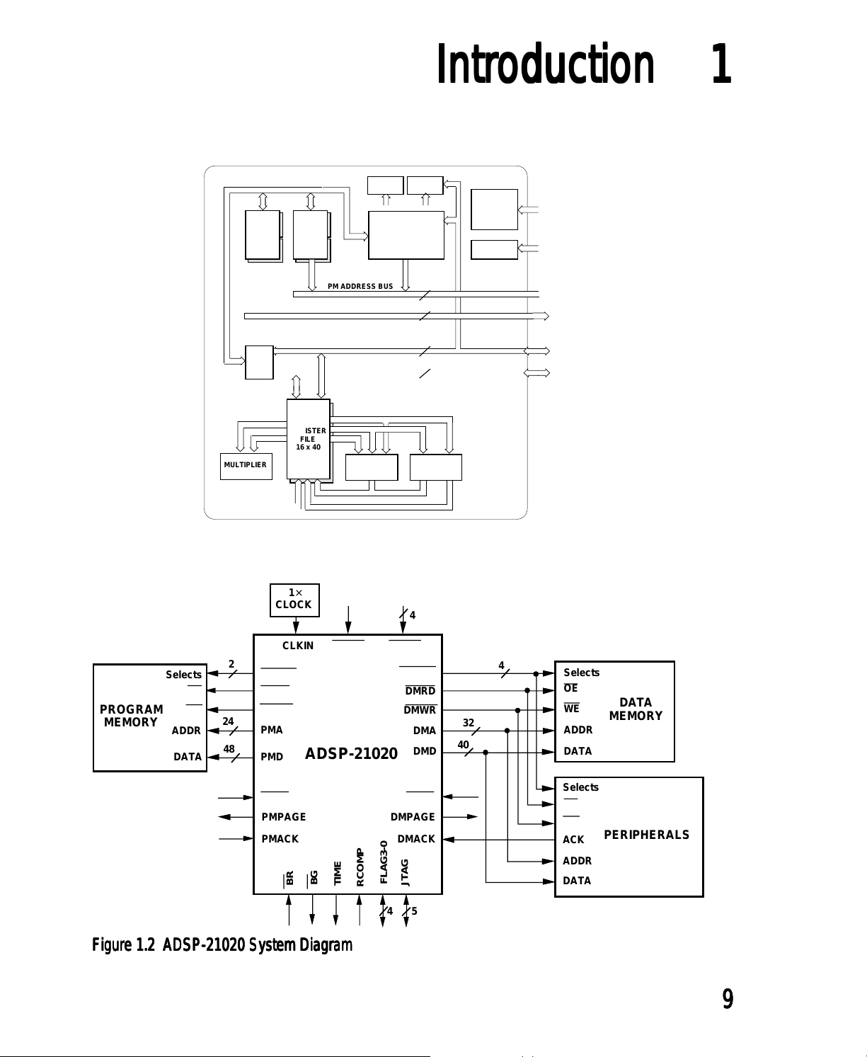
The ADSP-21020 is the first member of the ADSP-21000 family. It is a
complete implementation of the family base architecture. Figure 1.1 shows
the block diagram of the ADSP-21020 and Figure 1.2 shows a system
diagram.
ADSP-21020 DSPADSP-21020 DSP
ADSP-21020 DSP
ADSP-21020 DSPADSP-21020 DSP
88
8
88
Page 23
DAG 1
8 x 4 x 32
DAG 2
8 x 4 x 24
TIMER
PROGRAM
SEQUENCER
IntroductionIntroduction
Introduction
IntroductionIntroduction
CACHE
32 x 48
JTAG
TEST &
EMULATION
FLAGS
11
1
11
PM ADDRESS BUS
DM ADDRESS BUS
Bus
Connect
REGISTER
FILE
16 x 40
MULTIPLIER
Figure 1.1 ADSP-21020 Block DiagramFigure 1.1 ADSP-21020 Block Diagram
Figure 1.1 ADSP-21020 Block Diagram
Figure 1.1 ADSP-21020 Block DiagramFigure 1.1 ADSP-21020 Block Diagram
1×
CLOCK
CLKIN
2
PMS1-0
PMRD
PMWR
24
PMA
48
PMD
ADSP-21020
PROGRAM
MEMORY
Selects
OE
WE
ADDR
DATA
PM DATA BUS
DM DATA BUS
BARREL
SHIFTER
RESET IRQ3-0
DMS3-0
DMRD
DMWR
4
DMA
DMD
24
32
48
40
ALU
4
32
40
Selects
OE
WE
ADDR
DATA
DATA
MEMORY
PMTS
PMACK
BG
BR
Figure 1.2 ADSP-21020 System DiagramFigure 1.2 ADSP-21020 System Diagram
Figure 1.2 ADSP-21020 System Diagram
Figure 1.2 ADSP-21020 System DiagramFigure 1.2 ADSP-21020 System Diagram
TIMEXP
FLAG3-0
RCOMP
DMTS
DMPAGEPMPAGE
DMACK
JTAG
Selects
OE
WE
PERIPHERALS
ACK
ADDR
DATA
54
99
9
99
Page 24
11
1
11
IntroductionIntroduction
Introduction
IntroductionIntroduction
1.4.31.4.3
1.4.3
1.4.31.4.3
The ADSP-21060 SHARC (Super Harvard Architecture Computer) is a
single-chip 32-bit computer optimized for signal computing applications.
The ADSP-21060 SHARC has the following key features:
Four Megabit Configurable On-Chip SRAM
• Dual-Ported for Independent Access by Base Processor and DMA
• Configurable as Maximum 128K Words Data Memory (32-Bit),
Off-Chip Memory Interfacing
• 4 Gigawords Addressable (32-bit Address)
• Programmable Wait State Generation, Page-Mode DRAM Support
DMA Controller
ADSP-21060 SHARCADSP-21060 SHARC
ADSP-21060 SHARC
ADSP-21060 SHARCADSP-21060 SHARC
80K Words Program Memory (48-Bit), or Combinations of Both Up To
4 Mbits
1010
10
1010
Page 25

Trigonometric, Mathematical &Trigonometric, Mathematical &
Trigonometric, Mathematical &
Trigonometric, Mathematical &Trigonometric, Mathematical &
Transcendental FunctionsTranscendental Functions
Transcendental Functions
Transcendental FunctionsTranscendental Functions
This chapter contains listings and descriptions of several useful
trigonometric, mathematical and transcendental functions. The functions
are
Trigonometric
• sine/cosine approximation
• tangent approximation
• arctangent approximation
Mathematical
• square root
• square root with single precision
• inverse square root
• inverse square root with single precision
• division
22
2
22
Transcendental
• logarithm
• exponential
• power
2.12.1
2.1
2.12.1
The sine and cosine functions are fundamental operations commonly used
in digital signal processing algorithms , such as simple tone generation
and calculation of sine tables for FFTs. This section describes how to
calculate the sine and cosine functions.
This ADSP-210xx implementation of sin(x) is based on a min-max
polynomial approximation algorithm in the [CODY]. Computation of the
function sin(x) is reduced to the evaluation of a sine approximation over a
small interval that is symmetrical about the axis.
SINE/COSINE APPROXIMATION SINE/COSINE APPROXIMATION
SINE/COSINE APPROXIMATION
SINE/COSINE APPROXIMATION SINE/COSINE APPROXIMATION
1515
15
1515
Page 26
22
2
22
Trigonometric, Mathematical &Trigonometric, Mathematical &
Trigonometric, Mathematical &
Trigonometric, Mathematical &Trigonometric, Mathematical &
Transcendental FunctionsTranscendental Functions
Transcendental Functions
Transcendental FunctionsTranscendental Functions
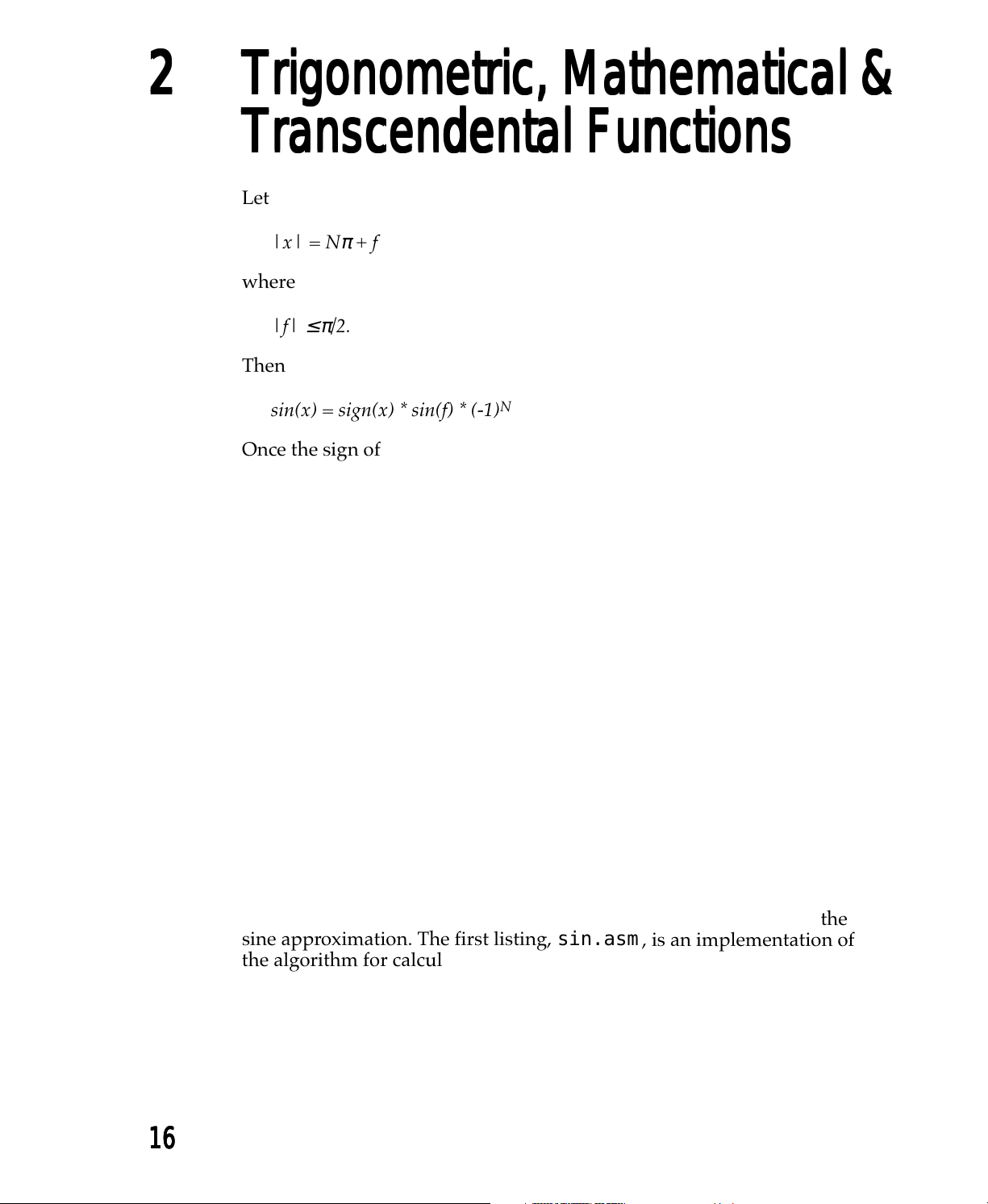
Let
π
≤ π
+ f
/2.
|x| = N
where
|f|
Then
sin(x) = sign(x) * sin(f) * (-1)
Once the sign of the input, x, is determined, the value of N can be
determined. The next step is to calculate f. In order to maintain the
maximum precision, f is calculated as follows
f = (|x| – xNC
The constants C
equal to pi (π). C
four decimal places beyond the precision of the ADSP-210xx.
For devices that represent floating-point numbers in 32 bits, Cody and
Waite suggest a seven term min-max polynomial of the form R(g) = g·P(g).
When expanded, the sine approximation for f is represented as
sin(f) = ((((((r
With sin(f) calculated, sin(x) can be constructed. The cosine function is
calculated similarly, using the trigonometric identity
cos(x) = sin(x +
) – xNC
1
and C2 are determined such that C
1
is determined such that C1 + C2 represents pi to three or
2
·f + r6) * f + r5) * f +r4) * f + r3) * f + r2) * f + r1) · f
7
π
/2)
N
2
is approximately
1
1616
16
1616
2.1.12.1.1
2.1.1
2.1.12.1.1
The two listings illustrate the sine approximation and the calling of the
sine approximation. The first listing, sin.asm
the algorithm for calculation of sines and cosines. The second listing,
sinetest.asm , is an example of a program that calls the sine
approximation.
Implementation Implementation
Implementation
Implementation Implementation
, is an implementation of
Page 27

Trigonometric, Mathematical &Trigonometric, Mathematical &
Trigonometric, Mathematical &
Trigonometric, Mathematical &Trigonometric, Mathematical &
Transcendental FunctionsTranscendental Functions
Transcendental Functions
Transcendental FunctionsTranscendental Functions
Implementation of the sine algorithm on ADSP-21000 family processors is
straightforward. In the first listing below,
defined. The first segment, defined with the .SEGMENT directive, contains
the assembly code for the sine/cosine approximation. The second segment
is a data segment that contains the constants necessary to perform this
approximation.
The code is structured as a called subroutine, where the parameter x is
passed into this routine using register F0. When the subroutine is finished
executing, the value sin(x) or cos(x) is returned in the same register, F0. The
variables, i_reg and l_reg
length register, in either data address generator on the ADSP-21000 family.
These registers are used in the program to point to elements of the data
table, sine_data . Elements of this table are accessed indirectly within
this program. Specifically, index registers I0 - I7 are used if the data table
containing all the constants is put in data memory and index registers I8 I15 are used if the data table is put in program memory. The variable mem
must be defined as program memory, PM , or data memory, DM .
, are specified as an index register and a
sin.asm , two segments are
22
2
22
The include file, asm_glob.h
and i_reg
The second listing, sinetest.asm
the cosine and sine routines.
There are two entry points in the subroutine, sin.asm . They are labeled
cosine and sine . Code execution begins at these labels. The calling
program uses these labels by executing the instruction
or
with the argument x in register F0. These calls are delayed branch calls
that efficiently use the instruction pipeline on the ADSP-21000 family. In a
delayed branch, the two instructions following the branch instruction are
executed prior to the branch. This prevents the need to flush an instruction
pipeline before taking a branch.
. You can alter these definitions to suit your needs.
call sine (db);
call cosine (db);
, contains definitions of mem, l_reg ,
, is an example of a routine that calls
1717
17
1717
Page 28
22
2
22
Trigonometric, Mathematical &Trigonometric, Mathematical &
Trigonometric, Mathematical &
Trigonometric, Mathematical &Trigonometric, Mathematical &
Transcendental FunctionsTranscendental Functions
Transcendental Functions
Transcendental FunctionsTranscendental Functions
2.1.22.1.2
2.1.2
2.1.22.1.2
2.1.2.12.1.2.1
2.1.2.1
2.1.2.12.1.2.1
/***************************************************************************
File Name
Version
0.03 7/4/90
Purpose
Equations Implemented
Calling Parameters
Return Values
Registers Affected
Code ListingsCode Listings
Code Listings
Code ListingsCode Listings
Sine/Cosine Approximation SubroutineSine/Cosine Approximation Subroutine
Sine/Cosine Approximation Subroutine
Sine/Cosine Approximation SubroutineSine/Cosine Approximation Subroutine
SIN.ASM
Subroutine to compute the Sine or Cosine values of a floating point input.
Y=SIN(X) or
Y=COS(X)
F0 = Input Value X=[6E-20, 6E20]
l_reg=0
F0 = Sine (or Cosine) of input Y=[-1,1]
F0, F2, F4, F7, F8, F12
i_reg
Cycle Count
38 Cycles
# PM Locations
34 words
# DM Locations
11 Words
***************************************************************************/
1818
18
1818
Page 29

Trigonometric, Mathematical &Trigonometric, Mathematical &
Trigonometric, Mathematical &
Trigonometric, Mathematical &Trigonometric, Mathematical &
Transcendental FunctionsTranscendental Functions
Transcendental Functions
Transcendental FunctionsTranscendental Functions
#include “asm_glob.h”
.SEGMENT/PM Assembly_Library_Code_Space;
.PRECISION=MACHINE_PRECISION;
#define half_PI 1.57079632679489661923
.GLOBAL cosine, sine;
/**** Cosine/Sine approximation program starts here. ****/
/**** Based on algorithm found in Cody and Waite. ****/
22
2
22
cosine:
i_reg=sine_data; /*Load pointer to data*/
F8=ABS F0; /*Use absolute value of input*/
F12=0.5; /*Used later after modulo*/
F2=1.57079632679489661923; /* and add PI/2*/
JUMP compute_modulo (DB); /*Follow sin code from here!*/
F4=F8+F2, F2=mem(i_reg,1);
F7=1.0; /*Sign flag is set to 1*/
sine:
i_reg=sine_data; /*Load pointer to data*/
F7=1.0; /*Assume a positive sign*/
F12=0.0; /*Used later after modulo*/
F8=ABS F0, F2=mem(i_reg,1);
F0=PASS F0, F4=F8;
IF LT F7=-F7; /*If input was negative, invert
sign*/
compute_modulo:
F4=F4*F2; /*Compute fp modulo value*/
R2=FIX F4; /*Round nearest fractional portion*/
BTST R2 BY 0; /*Test for odd number*/
IF NOT SZ F7=-F7; /*Invert sign if odd modulo*/
F4=FLOAT R2; /*Return to fp*/
F4=F4-F12, F2=mem(i_reg,1); /*Add cos adjust if necessary,
compute_f:
F12=F2*F4, F2=mem(i_reg,1); /*Compute XN*C1*/
F2=F2*F4, F12=F8-F12; /*Compute |X|-XN*C1, and
XN*C2*/
F8=F12-F2, F4=mem(i_reg,1); /*Compute f=(|X|-XN*C1)-
XN*C2*/
F12=ABS F8; /*Need magnitude for test*/
F4=F12-F4, F12=F8; /*Check for sin(x)=x*/
IF LT JUMP compute_sign; /*Return with result in F1*/
F4=XN*/
compute_R:
F12=F12*F12, F4=mem(i_reg,1);
(listing continues on next page)(listing continues on next page)
(listing continues on next page)
(listing continues on next page)(listing continues on next page)
1919
19
1919
Page 30

22
2
22
Trigonometric, Mathematical &Trigonometric, Mathematical &
Trigonometric, Mathematical &
Trigonometric, Mathematical &Trigonometric, Mathematical &
Transcendental FunctionsTranscendental Functions
Transcendental Functions
Transcendental FunctionsTranscendental Functions
LCNTR=6, DO compute_poly UNTIL LCE;
F4=F12*F4, F2=mem(i_reg,1); /*Compute sum*g*/
compute_poly:
compute_sign:
path*/
.ENDSEG;
.SEGMENT/SPACE Assembly_Library_Data_Space;
.PRECISION=MEMORY_PRECISION;
.VAR sine_data[11] =
F4=F2+F4; /*Compute sum=sum+next r*/
F4=F12*F4; /*Final multiply by g*/
RTS (DB), F4=F4*F8; /*Compute f*R*/
F12=F4+F8; /*Compute Result=f+f*R*/
F0=F12*F7; /*Restore sign of result*/
RTS; /*This return only for sin(eps)=eps
0.31830988618379067154, /*1/PI*/
3.14160156250000000000, /*C1, almost PI*/
-8.908910206761537356617E-6, /*C2, PI=C1+C2*/
9.536743164E-7, /*eps, sin(eps)=eps*/
-0.737066277507114174E-12, /*R7*/
0.160478446323816900E-9, /*R6*/
-0.250518708834705760E-7, /*R5*/
0.275573164212926457E-5, /*R4*/
-0.198412698232225068E-3, /*R3*/
0.833333333327592139E-2, /*R2*/
-0.166666666666659653; /*R1*/
.ENDSEG;
2020
20
2020
Page 31

Trigonometric, Mathematical &Trigonometric, Mathematical &
Trigonometric, Mathematical &
Trigonometric, Mathematical &Trigonometric, Mathematical &
Transcendental FunctionsTranscendental Functions
Transcendental Functions
Transcendental FunctionsTranscendental Functions
Listing 2.1 sin.asmListing 2.1 sin.asm
Listing 2.1 sin.asm
Listing 2.1 sin.asmListing 2.1 sin.asm
22
2
22
2.1.2.22.1.2.2
2.1.2.2
2.1.2.22.1.2.2
/
*********************************************************************************
File Name
SINTEST.ASM
Purpose
Example calling routine for the sine function.
*********************************************************************************/
#include “asm_glob.h”;
#include “def21020.h”;
#define N 4
#define PIE 3.141592654
.SEGMENT/DM dm_data; /* Declare variables in data memory
*/
.VAR input[N]= PIE/2, PIE/4, PIE*3/4, 12.12345678; /* test data */
.VAR output[N] /* results here */
.VAR correct[N]=1.0, .707106781, .707106781, -.0428573949; /* correct results
*/
.ENDSEG;
.SEGMENT/PM
Example Calling RoutineExample Calling Routine
Example Calling Routine
Example Calling RoutineExample Calling Routine
pm_rsti; /* The reset vector resides in this space */
DMWAIT=0x21; /* Set data memory waitstates to zero */
PMWAIT=0x21; /* Set program memory waitstates to zero */
JUMP start;
.ENDSEG;
.EXTERN sine;
.SEGMENT/PM pm_code;
start:
bit set mode2 0x10; nop; read cache 0; bit clr mode2 0x10;
M1=1;
B0=input;
L0=0;
I1=output;
L1=0;
lcntr=N, do calcit until lce;
CALL sine (db);
l_reg=0;
f0=dm(i0,m1);
calcit:
dm(i1,m1)=f0;
end:
2121
21
2121
Page 32

22
2
22
Trigonometric, Mathematical &Trigonometric, Mathematical &
Trigonometric, Mathematical &
Trigonometric, Mathematical &Trigonometric, Mathematical &
Transcendental FunctionsTranscendental Functions
Transcendental Functions
Transcendental FunctionsTranscendental Functions
.ENDSEG;
Listing 2.2 sintest.asmListing 2.2 sintest.asm
Listing 2.2 sintest.asm
Listing 2.2 sintest.asmListing 2.2 sintest.asm
2.22.2
2.2
2.22.2
The tangent function is one of the fundamental trigonometric signal
processing operations. This section shows how to approximate the tangent
function in software. The algorithm used is taken from [CODY].
Tan(x) is calculated in three steps:
1. The argument x (which may be any real value) is reduced to a
related argument f with a magnitude less than π/4 (that is, t has a
range of ± π/2).
2. Tan(f) is computed using a min-max polynomial approximation.
3. The desired function is reconstructed.
2.2.12.2.1
2.2.1
2.2.12.2.1
The implementation of the tangent approximation algorithm uses 38
instruction cycles and consists of three logical steps.
IDLE;
TANGENT APPROXIMATIONTANGENT APPROXIMATION
TANGENT APPROXIMATION
TANGENT APPROXIMATIONTANGENT APPROXIMATION
Implementation Implementation
Implementation
Implementation Implementation
2222
22
2222
First, the argument x is reduced to the argument f. This argument
reduction is done in the sections labeled compute_modulo and
compute_f
The factor
any floating-point value) to f (which is a normalized value with a range of
± π/2). To get an accurate result, the constants C
C
+ C
1
2
precision. The value C
added to C
Notice that in the argument reduction, the assembly instructions are all
multifunction instructions. ADSP-21000 family processors can execute a
data move or a register move in parallel with a computation. Because
multifunction instructions execute in a single cycle, the overhead for the
memory move is eliminated.
.
π
/2 is required in the computation to reduce x (which may be
and C2 are chosen so that
1
approximates π/2 to three or four decimal places beyond machine
is chosen to be close to π/2 and C2 is a factor that is
1
that results in a very accurate representation of π/2.
1
Page 33

Trigonometric, Mathematical &Trigonometric, Mathematical &
Trigonometric, Mathematical &
Trigonometric, Mathematical &Trigonometric, Mathematical &
Transcendental FunctionsTranscendental Functions
Transcendental Functions
Transcendental FunctionsTranscendental Functions
A special case is if tan(x) = x. This occurs when the absolute value of f is
less than epsilon. This value is very close to 0. In this case, a jump is
executed and the tangent function is calculated using the values of f and 1
in the final divide.
The second step is to approximate the tangent function using a min-max
polynomial expansion. Two calculations are performed, the calculation of
P(g) and the calculation of Q(g), where g is just f * f. Four coefficients are
used in calculation of both P(g) and Q(g). The section labeled compute_P
makes this calculation:
P(g) = ((p3 * g + p2) * g + p1) * g *f
Where g = f*f and f is the reduced argument of x. The value f * P(g) is
stored in the register F8.
22
2
22
The section labeled compute_Q
Q(g) = ((q
The third step in the calculation of the tangent function is to divide P(g) by
Q(g). If the argument, f, is even, then the tangent function is
tan(f) = f * P(g)/Q(g)
If the argument, f, is odd then the tangent function is
tan(f) = –f * P(g)/Q(g)
Finally, the value N is multiplied in and the reconstructed function tan(x)
is returned in the register F0.
*g + q2)*g + q1) * g + q
3
, makes this calculation:
0
2323
23
2323
Page 34

22
2
22
Similarly, the cotangent function is easily calculated by inverting the polynomial
cotan(f) = Q(g)/–f * P(g)
Trigonometric, Mathematical &Trigonometric, Mathematical &
Trigonometric, Mathematical &
Trigonometric, Mathematical &Trigonometric, Mathematical &
Transcendental FunctionsTranscendental Functions
Transcendental Functions
Transcendental FunctionsTranscendental Functions
2.2.22.2.2
2.2.2
2.2.22.2.2
/
*********************************************************************************
File Name
Version
Purpose
Equations Implemented
Calling Parameters
Return Values
Registers Affected
Code Listing–Tangent SubroutineCode Listing–Tangent Subroutine
Code Listing–Tangent Subroutine
Code Listing–Tangent SubroutineCode Listing–Tangent Subroutine
TAN.ASM
Version 0.03 7/5/90
Subroutine to compute the tangent of a floating point input.
Y=TAN(X)
F0 = Input Value X=[6E-20, 6E20]
l_reg = 0 (usually L3)
F0 = tangent of input X
F0, F1, F2, F4, F7, F8, F12
i_reg (usually I3)
Cycle Count
2424
24
2424
38 Cycles
Page 35

Trigonometric, Mathematical &Trigonometric, Mathematical &
Trigonometric, Mathematical &
Trigonometric, Mathematical &Trigonometric, Mathematical &
Transcendental FunctionsTranscendental Functions
Transcendental Functions
Transcendental FunctionsTranscendental Functions
# PM Locations
# DM Locations
*********************************************************************************/
#include “asm_glob.h”
.SEGMENT/PM Assembly_Library_Code_Space;
.PRECISION=MACHINE_PRECISION;
.GLOBAL tan;
22
2
22
tan: i_reg=tangent_data;
F8=PASS F0, F2=mem(i_reg,1); /* Use absolute value of input
*/
compute_modulo:
F4=F8*F2, F1=F0; /* Compute fp modulo value */
R2=FIX F4, F12=mem(i_reg,1); /* Rnd nearest fractional
F4=FLOAT R2, R0=R2; /* Return to fp */
compute_f:
F12=F12*F4, F2=mem(i_reg,1); /* Compute XN*C1 */
F2=F2*F4, F12=F8-F12; /* Compute X-XN*C1, and XN*C2
*/
F8=F12-F2, F4=mem(i_reg,1); /* Compute f=(X-XN*C1)-XN*C2
*/
F12=ABS F8, F7=F8;
F4=F12-F4, F12=mem(i_reg,1); /* Check for TAN(x)=x */
IF LT JUMP compute_quot; /* Compute quotient with NUM=f
compute_P:
F12=F8*F8, F4=mem(i_reg,1); /* g=f*f */
F4=F12*F4, F2=mem(i_reg,1); /* Compute p3*g */
F4=F2+F4; /* Compute (p3*g + p2) */
F4=F12*F4, F2=mem(i_reg,1); /* Compute (p3*g + p2)*g */
F4=F2+F4; /* Compute (p3*g + p2)*g + p1 */
F4=F12*F4; /* Compute
F4=F4*F8; /* Compute
F8=F4+F8, F4=mem(i_reg,1); /* Compute f*P(g) */
portion */
DEN=1 */
((p3*g + p2)*g + p1)*g */
((p3*g + p2)*g +p1)*g*f */
(listing continues on next page)(listing continues on next page)
(listing continues on next page)
(listing continues on next page)(listing continues on next page)
2525
25
2525
Page 36

22
2
22
Trigonometric, Mathematical &Trigonometric, Mathematical &
Trigonometric, Mathematical &
Trigonometric, Mathematical &Trigonometric, Mathematical &
Transcendental FunctionsTranscendental Functions
Transcendental Functions
Transcendental FunctionsTranscendental Functions
compute_Q:
F4=F12*F4, F2=mem(i_reg,1); /* Compute sum*g */
F4=F2+F4; /* Compute sum=sum+next q */
F4=F12*F4, F2=mem(i_reg,1); /* Compute sum*g */
F4=F2+F4; /* Compute sum=sum+next q */
F4=F12*F4, F2=mem(i_reg,1); /* Compute sum*g */
F12=F2+F4, F7=F8; /* Compute sum=sum+next q */
compute_quot:
BTST R0 BY 0; /* Test LSB */
IF NOT SZ F12=-F7, F7=F12; /* SZ true if even value*/
F0=RECIPS F12; /* Get 4 bit seed R0=1/D */
F12=F0*F12, F11=mem(i_reg,1); /* D(prime) = D*R0 */
F7=F0*F7, F0=F11-F12; /* F0=R1=2-D(prime), F7=N*R0
*/
F12=F0*F12; /* F12=D(prime)=D(prime)*R1 */
F7=F0*F7, F0=F11-F12; /* F7=N*R0*R1, F0=R2=2-
D(prime) */
RTS (DB), F12=F0*F12; /* F12=D(prime)=D(prime)*R2 */
F7=F0*F7, F0=F11-F12; /* F7=N*R0*R1*R2,
F0=F0*F7; /* F7=N*R0*R1*R2*R3 */
.ENDSEG;
F0=R3=2-D(prime)*/
.SEGMENT/SPACE Assembly_Library_Data_Space;
.PRECISION=MEMORY_PRECISION;
.VAR tangent_data[13] = 0.6366197723675834308, /* 2/PI */
2626
26
2626
1.57080078125, /* C1, almost PI/2 */
-4.454455103380768678308E-6, /* C2, PI/2=C1+C2 */
9.536743164E-7, /* eps, TAN(eps)=eps */
1.0, /* Used in one path */
-0.7483634966612065149E-5, /* P3 */
0.2805918241169988906E-2, /* P2 */
-0.1282834704095743847, /* P1 */
Page 37

Trigonometric, Mathematical &Trigonometric, Mathematical &
Trigonometric, Mathematical &
Trigonometric, Mathematical &Trigonometric, Mathematical &
Transcendental FunctionsTranscendental Functions
Transcendental Functions
Transcendental FunctionsTranscendental Functions
-0.2084480442203870948E-3, /* Q3 */
0.2334485282206872802E-1, /* Q2 */
-0.4616168037429048840, /* Q1 */
1.0, /* Q0 */
2.0; /* Used in divide */
.ENDSEG;
Listing 2.3 tan.asmListing 2.3 tan.asm
Listing 2.3 tan.asm
Listing 2.3 tan.asmListing 2.3 tan.asm
22
2
22
2.32.3
2.3
2.32.3
The arctangent function is one of the fundamental trigonometric signal
processing operations. Arctangent is often used in the calculation of the
phase of a signal and in the conversion between Cartesian and polar data
representations.
This section shows how to approximate the arctangent function in
software. The algorithm used is taken from [CODY].
Calculation of atan(x) is done in three steps:
1. The argument x (which may be any real value) is reduced to a
2. Atan(f) is computed using a rational expression.
3. The desired function is reconstructed.
2.3.12.3.1
2.3.1
2.3.12.3.1
This implementation of the tangent approximation algorithm uses 82
instruction cycles, in the worst case. It follows the three logical steps listed
above.
ARCTANGENT APPROXIMATIONARCTANGENT APPROXIMATION
ARCTANGENT APPROXIMATION
ARCTANGENT APPROXIMATIONARCTANGENT APPROXIMATION
related argument f with a magnitude less than or equal to 2– R(3).
ImplementationImplementation
Implementation
ImplementationImplementation
The assembly code module can be called to compute either of two
functions, atan or atan2
of an argument x. The atan2 function returns the arctangent of y/x. This
form
. The atan function returns the arctangent
2727
27
2727
Page 38

22
2
22
Trigonometric, Mathematical &Trigonometric, Mathematical &
Trigonometric, Mathematical &
Trigonometric, Mathematical &Trigonometric, Mathematical &
Transcendental FunctionsTranscendental Functions
Transcendental Functions
Transcendental FunctionsTranscendental Functions
H=atan(y/x)
is especially useful in phase calculations.
First, the argument x is reduced to the argument f. This argument
reduction relies on the symmetry of the arctangent function by using the
identity
arctan(x) = –arctan(–x)
The use of this identity guarantees that approximation uses a nonnegative x. For values that are greater than one, a second identity is used
in argument reduction
π
arctan(x) =
The reduction of x to the argument F is complete with the identity
/2 – arctan (1/x)
π
arctan(x) =
where
f = (x – (R(3) – 1) / (R(3) + x)
Just like tangent approximation, the second step in the arctangent
calculation is computing a rational expression of the form
R = g * P(g) / Q(g)
where
g * P(g) = (P1 * g + P0) * g
/6 + arctan(f)
2828
28
2828
Page 39

Trigonometric, Mathematical &Trigonometric, Mathematical &
Trigonometric, Mathematical &
Trigonometric, Mathematical &Trigonometric, Mathematical &
Transcendental FunctionsTranscendental Functions
Transcendental Functions
Transcendental FunctionsTranscendental Functions
and
Q(g) = (g + q1) * g + Q0
22
2
22
Notice that an eight-cycle macro, divide
used several times in the program.
The final step is to reconstruct the atan(x) from the atan(f) calculation.
2.3.22.3.2
2.3.2
2.3.22.3.2
/
*********************************************************************************
File Name
Version
Purpose
Equations Implemented
where H is in radians
Calling Parameters
Listing–Arctangent Subroutine Listing–Arctangent Subroutine
Listing–Arctangent Subroutine
Listing–Arctangent Subroutine Listing–Arctangent Subroutine
ATAN.ASM
Version 0.01 3/20/91
Subroutine to compute the arctangent values of a floating point input.
atan- H=ATAN(Y)
atan2- H=ATAN(Y/X)
F0 = Input Value Y=[6E-20, 6E20]
F1 = Input Value X=[6E-20, 6E20] (atan2 only)
l_reg=0
, is implemented for division. This macro is
Return Values
F0 = ArcTangent of input
=[-pi/2,pi/2] for atan
=[-pi,pi] for atan2
Registers Affected
F0, F1, F2, F4, F7, F8, F11, F12, F15
i_reg
ms_reg
(listing continues on next page)(listing continues on next page)
(listing continues on next page)
(listing continues on next page)(listing continues on next page)
2929
29
2929
Page 40

22
2
22
Cycle Count
# PM Locations
# DM Locations
*********************************************************************************/
/* The divide Macro used in the arctan routine*/
/* -----------------------------------------------------------------------------
------DIVIDE - Divide Macro
Register Usage:
q = f0-f15 Quotient
n = f4-f7 Numerator
d = f12-f15 Denominator
two = f8-f11 must have 2.0 pre-stored
tmp = f0-f3
Trigonometric, Mathematical &Trigonometric, Mathematical &
Trigonometric, Mathematical &
Trigonometric, Mathematical &Trigonometric, Mathematical &
Transcendental FunctionsTranscendental Functions
Transcendental Functions
Transcendental FunctionsTranscendental Functions
atan 61 Cycles maximum
atan2 82 cycles maximum
Indirectly affected registers:
ASTAT,STKY
Looping: none
Special Cases:
q may be any register, all others must be distinct.
Cycles: 8
Created: 3/19/91
--------------------------------------------------------------------------------
-----*/
#define DIVIDE(q,n,d,two,tmp) \
n=RECIPS d, tmp=n; /* Get 8 bit seed R0=1/D*/ \
d=n*d; /* D(prime) = D*R0*/ \
tmp=tmp*n, n=two-d; /* N=2-D(prime), TMP=N*R0*/ \
d=n*d; /* D=D(prime)=D(prime)*R1*/ \
tmp=tmp*n, n=two-d; /* TMP=N*R0*R1, N=R2=2-D(prime)*/ \
d=n*d; /* D=D(prime)=D(prime)*R2*/ \
tmp=tmp*n, n=two-d; /* TMP=N*R0*R1*R2, N=R3=2-D(prime)*/ \
q=tmp*n
3030
30
3030
Page 41

Trigonometric, Mathematical &Trigonometric, Mathematical &
Trigonometric, Mathematical &
Trigonometric, Mathematical &Trigonometric, Mathematical &
Transcendental FunctionsTranscendental Functions
Transcendental Functions
Transcendental FunctionsTranscendental Functions
#include “asm_glob.h”
.SEGMENT/PM Assembly_Library_Code_Space;
.PRECISION=MACHINE_PRECISION;
.GLOBAL atan, atan2;
atan2: i_reg=atan_data;
F11= 2.0;
F2= 0.0;
F1=PASS F1;
IF EQ JUMP denom_zero; /* if Denom. = 0, goto special
case*/
IF LT F2=mem(11,i_reg); /* if Denom. < 0, F2=pi (use at
end)*/
overflow_tst: R4=LOGB F0, F7=F0; /* Detect div overflow for atan2*/
R1=LOGB F1, F15=F1;
R1=R4-R1; /* Roughly exp. of quotient*/
R4=124; /* Max exponent - 3*/
COMP(R1,R4);
IF GE JUMP overflow; /* Over upper range? Goto overflow*/
R4=-R4;
COMP(R1,R4);
IF LE JUMP underflow; /* Over lower range? Goto
underflow*/
22
2
22
do_division: DIVIDE(F0,F7,F15,F11,F1);
JUMP re_entry (DB);
atan: R10= 0; /* Flags multiple of pi to add at
end*/
F15=ABS F0;
i_reg=atan_data; /* This init is redundant for
atan2f*/
F11= 2.0; /* Needed for divide*/
F2= 0.0; /* Result is not in Quad 2 or
3 */
re_entry: F7 = 1.0;
COMP(F15,F7), F4=mem(0,i_reg); /* F4=2-sqrt(3)*/
IF LE JUMP tst_f; /* If input<=1, do arctan(input)*/
DIVIDE(F15,F7,F15,F11,F1); /* do x=1/x*/
R10 = 2; /* signal to add const at
end*/
/* else do arctan(1/input)+const*/
(listing continues on next page)(listing continues on next page)
(listing continues on next page)
(listing continues on next page)(listing continues on next page)
3131
31
3131
Page 42

22
2
22
tst_f: COMP(F15,F4); /* Note F4 prev. loaded from memory*/
IF LT JUMP tst_for_eps;
R10=R10+1, F4=mem(1,i_reg); /* F4=sqrt(3)*/
F12=F4*F15;
F7=F12-F7; /* F7=F12-1.0*/
F15=F4+F15;
DIVIDE(F15,F7,F15,F11,F1); /* = (sqrt(3)*x-1)/(x+sqrt(3))*/
tst_for_eps: F7=ABS F15, F4=mem(2,i_reg); /* F4=eps (i.e. small)*/
COMP(F7,F4);
IF LE JUMP tst_N; /* if x<=eps, then h=x*/
F1=F15*F15, F4=mem(3,i_reg); /* else . . .*/
F7=F1*F4, F4=mem(4,i_reg);
F7=F7+F4, F4=mem(5,i_reg);
F7=F7*F1;
F12=F1+F4, F4=mem(6,i_reg);
F12=F12*F1;
F12=F12+F4;
DIVIDE(F7,F7,F12,F11,F1); /* e=((p1*x^2 +p0)x^2)/(x^2
+q1)x^2+q0*/
F7=F7*F15;
F15=F7+F15; /* h=e*x+x*/
Trigonometric, Mathematical &Trigonometric, Mathematical &
Trigonometric, Mathematical &
Trigonometric, Mathematical &Trigonometric, Mathematical &
Transcendental FunctionsTranscendental Functions
Transcendental Functions
Transcendental FunctionsTranscendental Functions
tst_N: R1=R10-1, R7=mem(i_reg,7); /* if R10 > 1, h=-h; dummy read*/
ms_reg=R10;
IF GT F15=-F15;
F4 = mem(ms_reg,i_reg); /* index correct angle addend to h
*/
F15=F15+F4; /* h=h+ a*pi */
tst_sign_y: F2=PASS F2; /* if (atan2f denom <0) h=pi-h else
h=h */
IF NE F15=F2-F15;
tst_sign_x: RTS (DB), F0=PASS F0; /* if (numer<0) h=-h else h=h*/
IF LT F15=-F15;
F0=PASS F15; /* return with result in F0!*/
underflow: JUMP tst_sign_y (DB);
F15=0;
NOP;
overflow: JUMP tst_sign_x (DB);
F15=mem(9,i_reg); /* Load pi/2*/
NOP;
denom_zero: F0=PASS F0; /* Careful: if Num !=0, then
overflow*/
IF NE JUMP overflow;
error: RTS; /* Error: Its a 0/0!*/
3232
32
3232
Page 43
Trigonometric, Mathematical &Trigonometric, Mathematical &
Trigonometric, Mathematical &
Trigonometric, Mathematical &Trigonometric, Mathematical &
Transcendental FunctionsTranscendental Functions
Transcendental Functions
Transcendental FunctionsTranscendental Functions
.ENDSEG;
.SEGMENT/SPACE Assembly_Library_Data_Space;
.PRECISION=MEMORY_PRECISION;
.VAR atan_data[11] = 0.26794919243112270647, /* 2-sqrt(3) */
1.73205080756887729353, /* sqrt(3) */
0.000244140625, /* eps */
-0.720026848898E+0, /* p1 */
-0.144008344874E+1, /* p0 */
0.475222584599E+1, /* q1 */
0.432025038919E+1, /* q0 */
0.00000000000000000000, /* 0*pi */
0.52359877559829887308, /* pi/6 */
1.57079632679489661923, /* pi/2 */
1.04719755119659774615, /* pi/3 */
3.14159265358979323846; /* pi */
.ENDSEG;
22
2
22
Listing 2.4 atan.asmListing 2.4 atan.asm
Listing 2.4 atan.asm
Listing 2.4 atan.asmListing 2.4 atan.asm
2.42.4
2.4
2.42.4
An ADSP-21000 family DSP can perform the square root function, sqrt(y),
and the inverse square root, isqrt(y), quickly and with a high degree of
precision. These functions are typically used to calculate magnitude
functions of FFT outputs, to implement imaging and graphics algorithms,
and to use the DSP as a fast math coprocessor.
A square root exists (and can be calculated) for every non-negative floatingpoint number. Calculating the square root of a negative number gives an
imaginary result. To calculate the square root of a negative number, take the
absolute value of the number and use sqrt(y) or isqrt(y) as defined in this
section. Remember that the result is really an imaginary number.
The ADSP-21000 family program that calculates isqrt(y) is based on the
Newton-Raphson iteration algorithm in [CAVANAGH]. Computation of the
function begins with a low-accuracy initial approximation. The Newton-
SQUARE ROOT & INVERSE SQUARE ROOTSQUARE ROOT & INVERSE SQUARE ROOT
SQUARE ROOT & INVERSE SQUARE ROOT
SQUARE ROOT & INVERSE SQUARE ROOTSQUARE ROOT & INVERSE SQUARE ROOT
APPROXIMATIONS APPROXIMATIONS
APPROXIMATIONS
APPROXIMATIONS APPROXIMATIONS
3333
33
3333
Page 44

22
2
22
Trigonometric, Mathematical &Trigonometric, Mathematical &
Trigonometric, Mathematical &
Trigonometric, Mathematical &Trigonometric, Mathematical &
Transcendental FunctionsTranscendental Functions
Transcendental Functions
Transcendental FunctionsTranscendental Functions
Raphson iteration is then used for successively more accurate
approximations.
Once isqrt(y) is calculated it only takes one additional operation to
calculate sqrt(y). Given the input, y, the square root, x=R(y), is determined
as follows
x = sqrt(y) = y * 1/sqrt(y)
Given an initial approximation xn for the inverse square root of y, isqrt(y),
the Newton-Raphson iteration is used to calculate a more accurate
approximation, x
n+1
.
Newton-Raphson iteration: x
The number of iterations determines the accuracy of the approximation.
For a 32-bit floating point representation with a 24-bit mantissa, two
iterations are sufficient to achieve an accuracy to ±1 LSB of precision. For
an extended 40-bit precision representation that has a 32-bit mantissa,
three iterations are needed.
For example, suppose that you need to calculate the square root of 30. If
you use 5.0 as an initial approximation of the square root, the inverse
square root approximation, 1/ 30, is 0.2. Therefore, given y=30 and
x
=0.2, one iteration yields
n
= (0.5) (0.2) (3 - (0.22 ) ( 30))
x
n+1
x
= 0.18
n+1
A second iteration using 0.18 as an input yields
= (0.5) (0.18) (3 – (0.182 ) (30))
x
n+2
x
= 0.18252
n+2
And finally a third iteration using 0.18252 as an input yields
= (0.5) (xn) (3 – (x
n+1
2
) (y))
n
3434
34
3434
= (0.5) (0.18252) (3 – (0.182522 ) (30))
x
n+2
x
= 0.182574161
n+2
Page 45

Trigonometric, Mathematical &Trigonometric, Mathematical &
Trigonometric, Mathematical &
Trigonometric, Mathematical &Trigonometric, Mathematical &
Transcendental FunctionsTranscendental Functions
Transcendental Functions
Transcendental FunctionsTranscendental Functions
Therefore the approximation of the inverse square root of 30 after three
iterations is 0.182574161. To calculate the square root, just multiply the
two numbers together
30 * 0.182574161 = 5.47722483
The actual square root of 30 is 5.477225575. If the initial approximation is
accurate to four bits, the final result is accurate to about 32 bits of
precision.
22
2
22
2.4.12.4.1
2.4.1
2.4.12.4.1
To implement the Newton-Raphson iteration method for calculating an
inverse square root on an ADSP-21000 processor, the first task is to
calculate the initial low-accuracy approximation.
The ADSP-21000 family instruction set includes the instruction RSQRTS
that, given the floating point input F
1/
√Fx. This seed, or low accuracy approximation, is determined by using
the six MSBs of the mantissa and the LSB of the unbiased exponent of Fx
to access a ROM-based look up table.
Note that the instruction RSQRTS only accepts inputs greater than zero.
A
±
number) or negative input returns an all 1's result. You can use
conditional logic to assure that the input value is greater than zero.
To calculate the seed for an input value stored in register F0, use the
following instruction:
Once you have the initial approximation, it is a easy to implement the
Newton-Raphon iteration in ADSP-21000 assembly code. With the
approximation now in F4 and with F1 and F8 initialized with the constants
0.5 and 3 respectively, one iteration of the Newton-Raphson is
ImplementationImplementation
Implementation
ImplementationImplementation
x, creates a 4-bit accurate seed for
Zero returns ±Infinity,
F4=RSQRTS F0; /*Fetch seed*/
±
Infinity returns ±Zero, and a NAN (not-a-
3535
35
3535
Page 46

22
2
22
implemented as follows:
F12=F4*F4; /* F12=X0^2 */
F12=F12*F0; /* F12=C*X0^2 */
F4=F2*F4, F12=F8-F12; /* F4=.5*X0, F10=3-C*X0^2 */
F4=F4*F12; /* F4=X1=.5*X0(3-C*X0^2) */
The register F4 contains a reasonably accurate approximation for the inverse square
root. Successive iterations are made by repeating the above four lines or code. The
square root of F0 is calculated by multiplying the approximation F4, by the initial
input F0:
F0=F4*F0; /* X=sqrt(Y)=Y/sqrt(Y) */
Trigonometric, Mathematical &Trigonometric, Mathematical &
Trigonometric, Mathematical &
Trigonometric, Mathematical &Trigonometric, Mathematical &
Transcendental FunctionsTranscendental Functions
Transcendental Functions
Transcendental FunctionsTranscendental Functions
2.4.22.4.2
2.4.2
2.4.22.4.2
There are four subroutine listings below that illustrate how to calculate sqrt(y) and
isqrt(y). Two are for single precision (24-bit mantissa), and two for extended precision
(32-bit mantissa).
2.4.2.12.4.2.1
2.4.2.1
2.4.2.12.4.2.1
/
***********************************************************************************
File Name
Code ListingsCode Listings
Code Listings
Code ListingsCode Listings
SQRT Approximation SubroutineSQRT Approximation Subroutine
SQRT Approximation Subroutine
SQRT Approximation SubroutineSQRT Approximation Subroutine
SQRT.ASM
3636
36
3636
Page 47

Trigonometric, Mathematical &Trigonometric, Mathematical &
Trigonometric, Mathematical &
Trigonometric, Mathematical &Trigonometric, Mathematical &
Transcendental FunctionsTranscendental Functions
Transcendental Functions
Transcendental FunctionsTranscendental Functions
Version
Version 0.02 7/6/90
Purpose
Subroutine to compute the square root of x using the 1/sqrt(x) approximation.
Equations Implemented
X = sqrt(Y) = Y/sqrt(Y)
Calling Parameters
F0 = Y Input Value
F8 = 3.0
F1 = 0.5
Return Values
F0 = sqrt(Y)
Registers Affected
F0, F4, F12
Cycle Count
14 Cycles
22
2
22
# PM Locations
# DM Locations
***********************************************************************************/
#include “asm_glob.h”
3737
37
3737
Page 48
22
2
22
.SEGMENT/PM pm_code;
.PRECISION=MACHINE_PRECISION;
.GLOBAL sqrt;
sqrt:
Trigonometric, Mathematical &Trigonometric, Mathematical &
Trigonometric, Mathematical &
Trigonometric, Mathematical &Trigonometric, Mathematical &
Transcendental FunctionsTranscendental Functions
Transcendental Functions
Transcendental FunctionsTranscendental Functions
F4=RSQRTS F0; /*Fetch seed*/
F12=F4*F4; /*F12=X0^2*/
F12=F12*F0; /*F12=C*X0^2*/
F4=F1*F4, F12=F8-F12; /*F4=.5*X0, F10=3-C*X0^2*/
F4=F4*F12; /*F4=X1=.5*X0(3-C*X0^2)*/
F12=F4*F4; /*F12=X1^2*/
F12=F12*F0; /*F12=C*X1^2*/
F4=F1*F4, F12=F8-F12; /*F4=.5*X1, F10=3-C*X1^2*/
F4=F4*F12; /*F4=X2=.5*X1(3-C*X1^2)*/
F12=F4*F4; /*F12=X2^2*/
F12=F12*F0; /*F12=C*X2^2*/
RTS (DB), F4=F1*F4, F12=F8-F12; /*F4=.5*X2, F10=3-C*X2^2*/
F4=F4*F12; /*F4=X3=.5*X2(3-C*X2^2)*/
F0=F4*F0; /*X=sqrt(Y)=Y/sqrt(Y)*/
.ENDSEG;
Listing 2.5 sqrt.asmListing 2.5 sqrt.asm
Listing 2.5 sqrt.asm
Listing 2.5 sqrt.asmListing 2.5 sqrt.asm
22
.4.2.2.4.2.2
2
.4.2.2
22
.4.2.2.4.2.2
/
*********************************************************************************
File Name
ISQRT Approximation SubroutineISQRT Approximation Subroutine
ISQRT Approximation Subroutine
ISQRT Approximation SubroutineISQRT Approximation Subroutine
ISQRT.ASM
3838
38
3838
Page 49

Trigonometric, Mathematical &Trigonometric, Mathematical &
Trigonometric, Mathematical &
Trigonometric, Mathematical &Trigonometric, Mathematical &
Transcendental FunctionsTranscendental Functions
Transcendental Functions
Transcendental FunctionsTranscendental Functions
Version
Version 0.02 7/6/90
Purpose
Subroutine to compute the inverse square root of x using the 1/
sqrt(x) approximation.
Equations Implemented
X = isqrt(Y) = 1/sqrt(Y)
Calling Parameters
F0 = Y Input Value
F8 = 3.0
F1 = 0.5
Return Values
F0 = isqrt(Y)
Registers Affected
F0, F4, F12
Cycle Count
13 Cycles
22
2
22
#PM Locations
#DM Locations
*********************************************************************************/
3939
39
3939
Page 50

22
2
22
#include “asm_glob.h”
.SEGMENT/PM pm_code;
.PRECISION=MACHINE_PRECISION;
.GLOBAL isqrt;
isqrt:
Trigonometric, Mathematical &Trigonometric, Mathematical &
Trigonometric, Mathematical &
Trigonometric, Mathematical &Trigonometric, Mathematical &
Transcendental FunctionsTranscendental Functions
Transcendental Functions
Transcendental FunctionsTranscendental Functions
F4=RSQRTS F0; /*Fetch seed*/
F12=F4*F4; /*F12=X0^2*/
F12=F12*F0; /*F12=C*X0^2*/
F4=F1*F4, F12=F8-F12; /*F4=.5*X0, F10=3-C*X0^2*/
F4=F4*F12; /*F4=X1=.5*X0(3-C*X0^2)*/
F12=F4*F4; /*F12=X1^2*/
F12=F12*F0; /*F12=C*X1^2*/
F4=F1*F4, F12=F8-F12; /*F4=.5*X1, F10=3-C*X1^2*/
F4=F4*F12; /*F4=X2=.5*X1(3-C*X1^2)*/
F12=F4*F4; /*F12=X2^2*/
F12=F12*F0; /*F12=C*X2^2*/
RTS (DB), F4=F1*F4, F12=F8-F12; /*F4=.5*X2, F10=3-C*X2^2*/
F4=F4*F12; /*F4=X3=.5*X2(3-C*X2^2)*/
/* =isqrt(Y)=1/sqrt(Y)*/
.ENDSEG;
Listing 2.6 isqrt.asmListing 2.6 isqrt.asm
Listing 2.6 isqrt.asm
Listing 2.6 isqrt.asmListing 2.6 isqrt.asm
2.4.2.32.4.2.3
2.4.2.3
2.4.2.32.4.2.3
/
*********************************************************************************
File Name
SQRTSGL Approximation SubroutineSQRTSGL Approximation Subroutine
SQRTSGL Approximation Subroutine
SQRTSGL Approximation SubroutineSQRTSGL Approximation Subroutine
SQRTSGL.ASM
4040
40
4040
Page 51

Trigonometric, Mathematical &Trigonometric, Mathematical &
Trigonometric, Mathematical &
Trigonometric, Mathematical &Trigonometric, Mathematical &
Transcendental FunctionsTranscendental Functions
Transcendental Functions
Transcendental FunctionsTranscendental Functions
Version
Version 0.02 7/6/90
Purpose
Subroutine to compute the square root of x to single-precision (24 bits
mantissa) using the 1/sqrt(x) approximation.
Equations Implemented
X = sqrtsgl(Y) = Y/sqrtsgl(Y)
Calling Parameters
F0 = Y Input Value
F8 = 3.0
F1 = 0.5
Return Values
F0 = sqrtsgl(Y)
Registers Affected
F0, F4, F12
Cycle Count
10 Cycles
22
2
22
4141
41
4141
Page 52

22
2
22
# PM Locations
# DM Locations
*********************************************************************************/
#include “asm_glob.h”
.SEGMENT/PM pm_code;
.PRECISION=MACHINE_PRECISION;
.GLOBAL sqrtsgl;
sqrtsgl:
.ENDSEG;
Trigonometric, Mathematical &Trigonometric, Mathematical &
Trigonometric, Mathematical &
Trigonometric, Mathematical &Trigonometric, Mathematical &
Transcendental FunctionsTranscendental Functions
Transcendental Functions
Transcendental FunctionsTranscendental Functions
F4=RSQRTS F0; /*Fetch seed*/
F12=F4*F4; /*F12=X0^2*/
F12=F12*F0; /*F12=C*X0^2*/
F4=F1*F4, F12=F8-F12; /*F4=.5*X0, F12=3-C*X0^2*/
F4=F4*F12; /*F4=X1=.5*X0(3-C*X0^2)*/
F12=F4*F4; /*F12=X1^2*/
F12=F12*F0; /*F12=C*X1^2*/
F4=F1*F4, F12=F8-F12; /*F4=.5*X1, F12=3-C*X1^2*/
F4=F4*F12; /*F4=X2=.5*X1(3-C*X1^2)*/
F0=F4*F0; /*X=sqrtsgl(Y)=Y/sqrtsgl(Y)*/
Listing 2.7 sqrtsgl.asmListing 2.7 sqrtsgl.asm
Listing 2.7 sqrtsgl.asm
Listing 2.7 sqrtsgl.asmListing 2.7 sqrtsgl.asm
2.4.2.42.4.2.4
2.4.2.4
2.4.2.42.4.2.4
/
*********************************************************************************
File Name
ISQRTSGL Approximation SubroutineISQRTSGL Approximation Subroutine
ISQRTSGL Approximation Subroutine
ISQRTSGL Approximation SubroutineISQRTSGL Approximation Subroutine
ISQRTSGL.ASM
4242
42
4242
Page 53

Trigonometric, Mathematical &Trigonometric, Mathematical &
Trigonometric, Mathematical &
Trigonometric, Mathematical &Trigonometric, Mathematical &
Transcendental FunctionsTranscendental Functions
Transcendental Functions
Transcendental FunctionsTranscendental Functions
Version
Version 0.02 7/6/90
Purpose
Subroutine to compute the inverse square root of x to single-precision (24
bits mantissa) using the 1/sqrt(x) approximation.
Equations Implemented
X = isqrtsgl(Y) = 1/sqrtsgl(Y)
Calling Parameters
F0 = Y Input Value
F8 = 3.0
F1 = 0.5
Return Values
F0 = isqrtsgl(Y)
Registers Affected
F0, F4, F12
Cycle Count
9 Cycles
22
2
22
4343
43
4343
Page 54

22
2
22
Trigonometric, Mathematical &Trigonometric, Mathematical &
Trigonometric, Mathematical &
Trigonometric, Mathematical &Trigonometric, Mathematical &
Transcendental FunctionsTranscendental Functions
Transcendental Functions
Transcendental FunctionsTranscendental Functions
# PM Locations
# DM Locations
*********************************************************************************/
#include “asm_glob.h”
.SEGMENT/PM pm_code;
.PRECISION=MACHINE_PRECISION;
.GLOBAL isqrtsgl;
isqrtsgl:
F4=RSQRTS F0; /*Fetch seed*/
F12=F4*F4; /*F12=X0^2*/
F12=F12*F0; /*F12=C*X0^2*/
F4=F1*F4, F12=F8-F12; /*F4=.5*X0, F12=3-C*X0^2*/
F4=F4*F12; /*F4=X1=.5*X0(3-C*X0^2)*/
F12=F4*F4; /*F12=X1^2*/
RTS(DB), F12=F12*F0; /*F12=C*X1^2*/
F4=F1*F4, F12=F8-F12; /*F4=.5*X1, F12=3-C*X1^2*/
F0=F4*F12; /*F4=X2=.5*X1(3-C*X1^2)*/
.ENDSEG;
/* =isqrtsgl(Y)=1/sqrtsgl(Y)*/
Listing 2.8 isqrtsgl.asmListing 2.8 isqrtsgl.asm
Listing 2.8 isqrtsgl.asm
Listing 2.8 isqrtsgl.asmListing 2.8 isqrtsgl.asm
2.52.5
2.5
2.52.5
The ADSP-21000 family instruction set includes the RECIPS instruction
to simplify the implementation of floating-point division.
2.5.12.5.1
2.5.1
2.5.12.5.1
The code performs floating-point division using an in iterative
convergence algorithm. The result is accurate to one LSB in whichever
format mode, 32-bit or 40-bit, is set (32-bit only for ADSP-21010). The
following inputs are required: F0 = numerator, F12= denominator,
F11 = 2.0. The quotients is returned in F0. (In the code listing, the two
highlighted instructions can be removed if only a ±1 LSB accurate singleprecision result is necessary.)
The algorithm is supplied with a startup seed which is a low-precision
reciprocal of the denominator. This seed is generated by the RECIPS
instruction. RECIPS creates an 8-bit accurate seed for 1/Fx, the reciprocal
of Fx. The mantissa of the seed is determined from a ROM table using the
7 MSBs (excluding the hidden bit) of the Fx mantissa as an index. The
unbiased exponent of the seed is calculated as the twos complement of the
DIVISIONDIVISION
DIVISION
DIVISIONDIVISION
ImplementationImplementation
Implementation
ImplementationImplementation
4444
44
4444
Page 55

Trigonometric, Mathematical &Trigonometric, Mathematical &
Trigonometric, Mathematical &
Trigonometric, Mathematical &Trigonometric, Mathematical &
Transcendental FunctionsTranscendental Functions
Transcendental Functions
Transcendental FunctionsTranscendental Functions
unbiased Fx exponent, decremented by one; that is, if e is the unbiased exponent of
Fx, then the unbiased exponent of Fn = –e – 1. The sign of the seed is the sign of the
input.
Fx is greater than +125, the result is
±
Zero returns ±Infinity and sets the overflow flag. If the unbiased exponent of
±
Zero. A NAN input returns an all 1's result.
22
2
22
2.5.22.5.2
2.5.2
2.5.22.5.2
/*
File Name
Version
Purpose
Algorithm.
Equations Implemented
Calling Parameters
F0 = N Input Value
F12 = D Input Value
F11 = 2.0
Return Values
F0 = Quotient of input
Registers Affected
F0, F7, F12
Cycle Count
8 Cycles (6 Cycles for single precision)
Code Listing–Division Subroutine Code Listing–Division Subroutine
Code Listing–Division Subroutine
Code Listing–Division Subroutine Code Listing–Division Subroutine
F.ASM
Version 0.03
An implementation of division using an Iterative Convergent Divide
Q = N/D
# PM Locations
# DM Locations
4545
45
4545
Page 56

22
2
22
Trigonometric, Mathematical &Trigonometric, Mathematical &
Trigonometric, Mathematical &
Trigonometric, Mathematical &Trigonometric, Mathematical &
Transcendental FunctionsTranscendental Functions
Transcendental Functions
Transcendental FunctionsTranscendental Functions
*/
#include “asm_glob.h”
.SEGMENT/PM Assembly_Library_Code_Space;
.PRECISION=MACHINE_PRECISION;
.GLOBAL divide;
divide: F0=RECIPS F12, F7=F0; /*Get 4 bit seed R0=1/D*/
F12=F0*F12; /*D(prime) = D*R0*/
F7=F0*F7, F0=F11-F12; /*F0=R1=2-D(prime), F7=N*R0*/
F12=F0*F12; /*F12=D(prime)=D(prime)*R1*/
F7=F0*F7, F0=F11-F12; /*F7=N*R0*R1, F0=R2=2D(prime)*/
/* Remove next two instructions for 1 LSB accurate single-precision
result */
RTS (DB), F12=F0*F12; {F12=D(prime)=D(prime)*R2}
F7=F0*F7, F0=F11-F12; {F7=N*R0*R1*R2, F0=R3=2-D(prime)}
F0=F0*F7; {F0=N*R0*R1*R2*R3}
.ENDSEG;
Listing 2.9 Divide..asmListing 2.9 Divide..asm
Listing 2.9 Divide..asm
Listing 2.9 Divide..asmListing 2.9 Divide..asm
2.62.6
2.6
2.62.6
Logarithms ( in base e, 2, and 10) can be approximated for any nonnegative floating point number. The Software Manual for the Elementary
Functions by William Cody and William Waite explains how the
computation of a logarithm involves three distinct steps:
The algorithm can calculate logarithms of any base (base e, 2, or 10); the
LOGARITHM APPROXIMATIONSLOGARITHM APPROXIMATIONS
LOGARITHM APPROXIMATIONS
LOGARITHM APPROXIMATIONSLOGARITHM APPROXIMATIONS
1. The given argument (or input) is reduced to a related argument in a
small, logarithmically symmetric interval about 1.
2. The logarithm is computed for this reduced argument.
3. The desired logarithm is reconstructed from its components.
4646
46
4646
Page 57

Trigonometric, Mathematical &Trigonometric, Mathematical &
Trigonometric, Mathematical &
Trigonometric, Mathematical &Trigonometric, Mathematical &
Transcendental FunctionsTranscendental Functions
Transcendental Functions
Transcendental FunctionsTranscendental Functions
code is identical until step three, so only one assembly-language module is
needed.
The first step is to take a given floating point input, Y, and reduce it to
Y=f * 2
N * loge(2) is the floating point exponent multiplied by loge(2), which is a
constant. The term loge(f) must be calculated. The definition of the variable
s is
Then
N
where 0.5 ≤f < 1. Given that X = log(Y), X also equals
X=loge(Y)
X=loge(f * 2N)
X=loge(f) + N*loge(2)
s = (f – 1) / (f + 1)
22
2
22
loge(f) = loge((1 + s) / (1 – s))
This equation is evaluated using a min-max rational approximation
detailed in [CODY]. The approximation is expressed in terms of the
auxiliary variable z = 2s.
Once the value of loge(f) is approximated, the equation
X = loge(f) + N*loge(2)
yields the solution for the natural (base-e) log of the input Y. To compute
the base-2 or base-10 logarithm, the result X is multiplied by a constant
equal to the reciprocal of loge(2), or loge(10), respectively.
2.6.12.6.1
2.6.1
2.6.12.6.1
LOGS.ASM is an assembly-language implementation of the logarithm
algorithm. This module has three entry points; a different base of
logarithm is computed depending on which entry point is used. The label
LOG is used for calling the algorithm to approximate the natural (base-e)
logarithm, while the labels LOG2 and LOG10 are used for base-2 and
base-10 approximations, respectively. When assembling the file
LOGS.ASM you can specify where coefficients are placed—either in data
memory (DM) or program memory (PM)— by using the -D
ImplementationImplementation
Implementation
ImplementationImplementation
identifier
4747
47
4747
Page 58

22
2
22
Trigonometric, Mathematical &Trigonometric, Mathematical &
Trigonometric, Mathematical &
Trigonometric, Mathematical &Trigonometric, Mathematical &
Transcendental FunctionsTranscendental Functions
Transcendental Functions
Transcendental FunctionsTranscendental Functions
switch at assembly time.
For example, to place the coefficients in data memory use the syntax
asm21k -DDM_DATA logs
To place the coefficients in program memory use the syntax
asm21k -DPM_DATA logs
The first step to compute any of the desired logarithms is to reduce the
floating point input Y to the form
Y=f * 2
The ADSP-21000 family supports the IEEE Standard 754/854 floating
point format. This format has a biased exponent and a significant with a
“hidden” bit of 1. The hidden bit, although not explicitly represented, is
implicitly presumed to exist and it offsets the exponent by one bit place.
For example, consider the floating point number 12.0. Using the IEEE
standard, this number is represented as 0.5 * 2
one and unbiasing the exponent, 12.0 is actually represented as 1.5 * 2
get to the format f * 2
get the format 0.75 * 2
our floating-point input. The exponent is then decremented, and the
mantissa is scaled to achieve the desired format.
Use the value of f to approximate the value of the auxiliary variable z. The
variable z is approximated using the following formula
z=znum/zden
where
znum = (f – 0.5) – 0.5
N
131
. By adding the hidden
4
. To
N
where 0.5 ≤ f < 1, you must scale 1.5 * 24 by two to
3
. The instruction LOGB extracts the exponent from
4848
48
4848
and
zden = (f * 0.5) – 0.5 for f>1/sqrt(2)
Page 59

Trigonometric, Mathematical &Trigonometric, Mathematical &
Trigonometric, Mathematical &
Trigonometric, Mathematical &Trigonometric, Mathematical &
Transcendental FunctionsTranscendental Functions
Transcendental Functions
Transcendental FunctionsTranscendental Functions
or
znum = f – 0.5 and
zden = znum * 0.5 + 0.5 for f <= 1/sqrt(2)
Once z is found, it is used to calculate the min-max rational approximation
R(z), which has the form
2
R(z) = z + z * r(z
The rational approximation r(z
2
) = w * A(w)/B(w)
r(z
where A(w) and B(w) are polynomials in w, with derived coefficients a0,
a1, and b0
)
2
) has been derived and for w=z2 is
22
2
22
A(w) = a1 * w + a0
B(w) = w + b0
R(z) is the approximation of loge(f) and the final step in the approximation
of loge(Y) is to add in N*loge(2). The coefficients C0 and C1 and the
exponent N are used to determine this value.
If only the natural logarithm is desired, then the algorithm is complete and
the natural log (ln(Y)) is returned in the register F0. If log2(Y) was needed,
then F0 is multiplied by 1/ln(2) or 1.442695041. If log10(Y) is needed, then
F0 is multiplied by 1/ln(10) or 0.43429448190325182765.
2.6.22.6.2
2.6.2
2.6.22.6.2
The listing for module LOGS.ASM is below. The calling routine uses the
appropriate label for the type of logarithm that is desired: LOG for
natural log (base-e), LOG2 for base-2 and LOG10 for base-10.
At assembly time, you must specify the memory space where the eight
coefficients are stored (Program or Data Memory ) by using either the
-DDM_DATA or -DPM_DATA switch. Attempts to assemble LOGS.ASM
without one of these switches result in an error.
2.6.2.12.6.2.1
2.6.2.1
2.6.2.12.6.2.1
Code ListingCode Listing
Code Listing
Code ListingCode Listing
Logarithm Approximation SubroutineLogarithm Approximation Subroutine
Logarithm Approximation Subroutine
Logarithm Approximation SubroutineLogarithm Approximation Subroutine
(listing continues on next page)(listing continues on next page)
(listing continues on next page)
(listing continues on next page)(listing continues on next page)
4949
49
4949
Page 60

22
2
22
/***************************************************************
File Name
Version
Purpose
Equations Implemented
Calling Parameters
Return Values
Trigonometric, Mathematical &Trigonometric, Mathematical &
Trigonometric, Mathematical &
Trigonometric, Mathematical &Trigonometric, Mathematical &
Transcendental FunctionsTranscendental Functions
Transcendental Functions
Transcendental FunctionsTranscendental Functions
LOGS.ASM
Version 0.03 8/6/90
revised 26-APR-91
Subroutine to compute the logarithm (bases 2,e, and 10) of its floating
point input.
Y=LOG(X) or
Y=LOG2(X) or
Y=LOG10(X)
F0 = Input Value
l_reg=0;
F0 = Logarithm of input
Registers Affected
F0, F1, F6, F7, F8, F10, F11, F12
i_reg
Computation Time
49 Cycles
#PM locations
#DM locations
***************************************************************/
#include “asm_glob.h”
.SEGMENT/PM Assembly_Library_Code_Space;
.PRECISION=MACHINE_PRECISION;
.GLOBAL log, log10, log2;
log2:
CALL logs_core (DB); /*Enter same routine in two cycles*/
R11=LOGB F0, F1=F0; /*Extract the exponent*/
F12=ABS F1; /*Get absolute value*/
RTS (DB);
F11=1.442695041; /*1/Log(2)*/
5050
50
5050
Page 61

Trigonometric, Mathematical &Trigonometric, Mathematical &
Trigonometric, Mathematical &
Trigonometric, Mathematical &Trigonometric, Mathematical &
Transcendental FunctionsTranscendental Functions
Transcendental Functions
Transcendental FunctionsTranscendental Functions
F0=F11*F0; /*F0 = log2(X)*/
log10:
CALL logs_core (DB); /*Enter same routine in two cycles*/
R11=LOGB F0, F1=F0; /*Extract the exponent*/
F12=ABS F1; /*Get absolute value*/
RTS (DB);
F11=0.43429448190325182765; /*1/Log(10)*/
F0=F11*F0; /*F12 = log10(X)*/
log:
R11=LOGB F0, F1=F0;
F12=ABS F1;
logs_core: i_reg=logs_data; /*Point to data array*/
R11=R11+1; /*Increment exponent*/
R7=-R11, F10=mem(i_reg,1); /*Negate exponent*/
F12=SCALB F12 BY R7; /*F12= .5<=f<1*/
COMP(F12,F10), F10=mem(i_reg,1); /*Compare f > C0*/
IF GT JUMP adjust_z (DB);
F7=F12-F10; /*znum = f-.5*/
F8=F7*F10; /*znum * .5*/
JUMP compute_r (DB);
F12=F8+F10; /*zden = znum * .5 + .5*/
R11=R11-1; /*N = N - 1*/
22
2
22
adjust_z:
F7=F7-F10; /*znum = f - .5 - .5*/
F8=F12*F10; /*f * .5*/
F12=F8+F10; /*zden = f * .5 + .5*/
compute_r:
F0=RECIPS F12; /*Get 4 bit seed R0=1/D*/
F12=F0*F12, F10=mem(i_reg,1); /*D(prime) = D*R0*/
F7=F0*F7, F0=F10-F12; /*F0=R1=2-D(prime), F7=N*R0*/
F12=F0*F12; /*F12=D(prime)=D(prime)*R1*/
F7=F0*F7, F0=F10-F12; /*F7=N*R0*R1, F0=R2=2-D(prime)*/
F12=F0*F12; /*F12=D(prime)=D(prime)*R2*/
F7=F0*F7, F0=F10-F12; /*F7=N*R0*R1*R2, F0=R3=2-D(prime)*/
F6=F0*F7; /*F7=N*R0*R1*R2*R3*/
F0=F6*F6, F8=mem(i_reg,1); /*w = z^2*/
F12=F8+F0, F8=mem(i_reg,1); /*B(W) = w + b0*/
F7=F8*F0, F8=mem(i_reg,1); /* w*a1*/
F7=F7+F8, F8=F0; /*A(W) = w * a1 + a0*/
F0=RECIPS F12; /*Get 4 bit seed R0=1/D*/
F12=F0*F12; /*D(prime) = D*R0*/
F7=F0*F7, F0=F10-F12; /*F0=R1=2-D(prime), F7=N*R0*/
F12=F0*F12; /*F12=D(prime)=D(prime)*R1*/
F7=F0*F7, F0=F10-F12; /*F7=N*R0*R1, F0=R2=2-D(prime)*/
5151
51
5151
Page 62

22
2
22
Trigonometric, Mathematical &Trigonometric, Mathematical &
Trigonometric, Mathematical &
Trigonometric, Mathematical &Trigonometric, Mathematical &
Transcendental FunctionsTranscendental Functions
Transcendental Functions
Transcendental FunctionsTranscendental Functions
F12=F0*F12; /*F12=D(prime)=D(prime)*R2*/
F7=F0*F7, F0=F10-F12; /*F7=N*R0*R1*R2, F0=R3=2-
D(prime)*/
F7=F0*F7; /*F7=N*R0*R1*R2*R3*/
F7=F7*F8; /*Compute r(z^2)=w*A(w)/B(w)*/
compute_R:
F7=F6*F7; /* z*r(z^2)*/
F12=F6+F7; /*R(z) = z + z * r(z^2)*/
F0=FLOAT R11, F7=mem(i_reg,1); /*F0=XN, F7=C2*/
F10=F0*F7, F7=mem(i_reg,1); /*F10=XN*C2, F7=C1*/
RTS (DB);
F7=F0*F7, F0=F10+F12; /*F0=XN*C2+R(z),
F7=XN*C1*/
F0=F0+F7; /*F0 = ln(X)*/
.ENDSEG;
.SEGMENT/SPACE Assembly_Library_Data_Space;
.VAR logs_data[8] = 0.70710678118654752440, /*C0 = sqrt(.5)*/
0.5, /*Constant used*/
2.0, /*Constant used*/
-5.578873750242, /*b0*/
0.1360095468621E-1, /*a1*/
-0.4649062303464, /*a0*/
-2.121944400546905827679E-4, /*C2*/
0.693359375; /*C1*/
.ENDSEG;
Listing 2.10 logs.asmListing 2.10 logs.asm
Listing 2.10 logs.asm
Listing 2.10 logs.asmListing 2.10 logs.asm
2.72.7
2.7
2.72.7
The exponential function (eX or exp(X)) of a floating point number is
computed by using an approximation technique detailed in the [CODY].
Cody and Waite explain how the computation of an exponent involves
three distinct steps.
The first step is to reduce a given argument (or input) to a related
argument in a small interval symmetric about the origin. If X is the input
value for which you wish to compute the exponent, let
Then
EXPONENTIAL APPROXIMATIONEXPONENTIAL APPROXIMATION
EXPONENTIAL APPROXIMATION
EXPONENTIAL APPROXIMATIONEXPONENTIAL APPROXIMATION
X = N*ln(C) + g
exp(X) = exp(g) * C
g ≤
N
ln(C)/2.
5252
52
5252
Page 63

Trigonometric, Mathematical &Trigonometric, Mathematical &
Trigonometric, Mathematical &
Trigonometric, Mathematical &Trigonometric, Mathematical &
Transcendental FunctionsTranscendental Functions
Transcendental Functions
Transcendental FunctionsTranscendental Functions
where C = 2, and N is calculated as X/ln(C). Since the accuracy of the
approximation critically depends on the accuracy of g, the effective
precision of the ADSP-210xx processor must be extended during the
calculation of g. Use the equation
g = (
X
– XN * C1) – XN * C
where C1 + C2 represent ln(C) to more than working precision, and XN is
the floating point representation of N. The values of C
precomputed and stored in program or data memory.
The second step is to compute the exponential for the reduced argument.
Since you have now calculated N and g, you must approximate exp(g).
Cody and Waite have derived coefficients (p1, q1, etc.) especially for the
approximation of exp(g)/2. The divide by two is added to counteract
wobbly precision. The approximation of exp(g)/2 is
2
and C2 are
1
22
2
22
R(g) = 0.5 + (g*P(z))/Q(z)- g(P(z))
where
g*P(z) = ((p1 * z) + p0) * g,
Q(z) = (q1 * z) + q0,
2
z = g
The third step is to reconstruct the desired function from its components.
The components of exp(X) are exp(g)=R(g), C=2, and N=X/ln(2). Therefore:
exp(X) = exp(g) * C
= R(g) * 2
Note that N was incremented by one due to the scaling that occurred in
the approximation of exp(g).
2.7.12.7.1
2.7.1
2.7.12.7.1
EXP.ASM is an implementation of the exponent approximation for the
ADSP-21000 family. When assembling the file EXP.ASM you can specify
where coefficients are placed—either in data memory (DM) or program
memory (PM)— by using the -D
time.
ImplementationImplementation
Implementation
ImplementationImplementation
N
(N+1)
identifier
switch at assembly
5353
53
5353
Page 64

22
2
22
Trigonometric, Mathematical &Trigonometric, Mathematical &
Trigonometric, Mathematical &
Trigonometric, Mathematical &Trigonometric, Mathematical &
Transcendental FunctionsTranscendental Functions
Transcendental Functions
Transcendental FunctionsTranscendental Functions
For example, to place the coefficients in data memory use the syntax
asm21k -DDM_DATA exp
To place the coefficients in program memory use the syntax
asm21k -DPM_DATA exp
Before the first step in the approximation of the exponential function is
performed, the floating-point input value is checked to assure that it is in
the allowable range. The floating-point input is limited by the machine
precision of the processor calculating the function. For the ADSP-21000
family, the largest number that can be represented is XMAX = 2
Therefore, the largest input to the function exp(X) is ln(XMAX), which is
approximately 88. The smallest positive floating point number that can be
represented is XMIN=2
as the largest negative input to the function exp(x). Therefore, comparisons
to ln(XMIN) and ln(XMAX) are the first instructions of the EXP.ASM
module. If these values are exceeded, the subroutine ends and returns
either an error (X > ln(XMAX)) or a very small number (X < ln(XMIN)).
–127
. Computing ln(XMIN) gives approximately –88
127
– 1LSB.
The code includes another comparison for the case where the input
produces the output 1. This only occurs when the input is equal to
0.000000001 or 1.0E-9. If the input equals this value, the subroutine ends
and returns a one.
The first step in the approximation is to compute g and N for the equation
exp(X) = exp(g) * 2
Where
N=X/ln(2)
g = (X - XN * C1) – XN * C
C1 = 0.693359375
C2 = –2.1219444005469058277E-4
Since multiplication requires fewer instructions than division, the constant
1/ln(2) is stored in memory along with the precomputed values of C
C
. XN is a floating point representation of N that can be easily computed
2
using the FIX and FLOAT conversion features of the ADSP-210xx
processors.
Given g and X
N
N
2
and
1
, it is simple to compute the approximation for exp(g)/2
5454
54
5454
Page 65

Trigonometric, Mathematical &Trigonometric, Mathematical &
Trigonometric, Mathematical &
Trigonometric, Mathematical &Trigonometric, Mathematical &
Transcendental FunctionsTranscendental Functions
Transcendental Functions
Transcendental FunctionsTranscendental Functions
using the constants and equations outlined in the [CODY].
R(g) = 0.5 + (g * P(z)) / Q(z) – g(P(z))
where
g*P(z) = ((p1 * z) + p0) * g,
Q(z) = (q1 * z) + q0
2
z = g
P1 = 0.59504254977591E–2
P0 = 0.24999999999992
Q2 = 0.29729363682238E-3
Q1 = 0.53567517645222E-1
Q0 = 0.5
Once R(g), the approximation for exp(g), is calculated, the approximation for exp(x) is
derived by using the following equation:
22
2
22
exp(X) = 2(approx(exp(g)/2)) * 2
= approx(exp(g)/2) * 2
= R(g) * 2
The SCALB instruction scales the floating point value of R(g) by the exponent N + 1.
2.7.22.7.2
2.7.2
2.7.22.7.2
/***************************************************************
File Name
Code Listings–Exponential SubroutineCode Listings–Exponential Subroutine
Code Listings–Exponential Subroutine
Code Listings–Exponential SubroutineCode Listings–Exponential Subroutine
EXP.ASM
(N+1)
N
(N+1)
(listing continues on next page)(listing continues on next page)
(listing continues on next page)
(listing continues on next page)(listing continues on next page)
5555
55
5555
Page 66

22
2
22
Version
Purpose
Equations Implemented
Calling Parameters
Return Values
Registers Affected
Computation Time
Trigonometric, Mathematical &Trigonometric, Mathematical &
Trigonometric, Mathematical &
Trigonometric, Mathematical &Trigonometric, Mathematical &
Transcendental FunctionsTranscendental Functions
Transcendental Functions
Transcendental FunctionsTranscendental Functions
Version 0.03 8/6/90
Modified 9/27/93
Subroutine to compute the exponential of its floating point input
Y=EXP(X)
F0 = Input Value
l_reg=0;
F0 = Exponential of input
F0, F1, F4, F7, F8, F10, F12
i_reg
38 Cycles
# PM locations
46 words
#DM locations
12 words (could be placed in PM instead)
***************************************************************/
#include “asm_glob.h”
.SEGMENT/PM Assembly_Library_Code_Space;
.PRECISION=MACHINE_PRECISION;
.GLOBAL exponential;
output_too_large: RTS (DB);
F0=10000; /*Set some error here*/
F0=10000;
output_too_small: RTS (DB);
F0 = .000001;
F0 = .000001;
output_one: RTS (DB);
F0 = 1.0;
F0 = 1.0;
exponential: i_reg=exponential_data; /*Skip one cycle after this*/
F1=PASS F0; /*Copy into F1*/
F12=ABS F1, F10=mem(i_reg,1); /*Fetch maximum input*/
COMP(F1,F10), F10=mem(i_reg,1); /*Error if greater than max*/
IF GT JUMP output_too_large; /*Return XMAX with error*/
COMP(F1,F10), F10=mem(i_reg,1); /*Test for input to small*/
IF LT JUMP output_too_small; /*Return 0 with error*/
COMP(F12,F10), F10=mem(i_reg,1); /*Check for output 1*/
5656
56
5656
Page 67

Trigonometric, Mathematical &Trigonometric, Mathematical &
Trigonometric, Mathematical &
Trigonometric, Mathematical &Trigonometric, Mathematical &
Transcendental FunctionsTranscendental Functions
Transcendental Functions
Transcendental FunctionsTranscendental Functions
IF LT JUMP output_one; /*Simply return 1*/
F12=F1*F10, F8=F1; /*Compute N = X/ln(C)*/
R4=FIX F12; /*Round to nearest*/
F4=FLOAT R4, F0=mem(i_reg,1); /*Back to floating point*/
compute_g: F12=F0*F4, F0=mem(i_reg,1); /*Compute
XN*C1*/
F0=F0*F4, F12=F8-F12; /*Compute |X|-XN*C1,
and XN*C2*/
F8=F12-F0, F0=mem(i_reg,1); /*Compute g=(|X|XN*C1)-XN*C2*/
compute_R: F10=F8*F8; /*Compute z=g*g*/
F7=F10*F0, F0=mem(i_reg,1); /*Compute p1*z*/
F7=F7+F0, F0=mem(i_reg,1); /*Compute p1*z + p0*/
F7=F8*F7; /*Compute g*P(z) =
(p1*z+p0)*g*/
F12=F0*F10, F0=mem(i_reg,1); /*Compute q2*z*/
F12=F0+F12, F8=mem(i_reg,1); /*Compute q2*z +
q1*/
F12=F10*F12; /*Compute (q2*z+q1)*z)*/
F12=F8+F12; /*Compute
Q(z)=(q2*z+q1)*z+q0*/
F12=F12-F7, F10=mem(i_reg,1); /*Compute Q(z) - g*P(z)*/
F0=RECIPS F12; /*Get 4 bit seed
R0=1/D*/
F12=F0*F12; /*D(prime) = D*R0*/
F7=F0*F7, F0=F10-F12; /*F0=R1=2-D(prime),
F7=N*R0*/
F12=F0*F12; /
*F12=D(prime)=D(prime)*R1*/
F7=F0*F7, F0=F10-F12; /*F7=N*R0*R1,
F0=R2=2-D(prime)*/
F12=F0*F12; /
*F12=D(prime)=D(prime)*R2*/
F7=F0*F7, F0=F10-F12; /*F7=N*R0*R1*R2,
F0=R3=2-D(prime)*/
F7=F0*F7; /*F7=N*R0*R1*R2*R3*/
F7=F7+F8; /*R(g) = .5 +
g*P(z))*/
R4=FIX F4; /*Get N in fixed point
again*/
RTS (DB);
R4=R4+1;
F0=SCALB F7 BY R4; /*R(g) * 2^(N+1)*/
.ENDSEG;
(g*P(z))/(Q(z)-
22
2
22
.SEGMENT/SPACE Assembly_Library_Data_Space;
.PRECISION=MEMORY_PRECISION;
.VAR exponential_data[12] = 88.0, /*BIGX */
-88.0, /*SMALLX*/
0.000000001, /*eps*/
1.4426950408889634074, /*1/ln(2.0)*/
0.693359375, /*C1*/
-2.1219444005469058277E-4, /*C2*/
0.59504254977591E-2, /*P1*/
0.24999999999992, /*P0*/
0.29729363682238E-3, /*Q2*/
5757
57
5757
Page 68

22
2
22
Trigonometric, Mathematical &Trigonometric, Mathematical &
Trigonometric, Mathematical &
Trigonometric, Mathematical &Trigonometric, Mathematical &
Transcendental FunctionsTranscendental Functions
Transcendental Functions
Transcendental FunctionsTranscendental Functions
0.53567517645222E-1, /*Q1*/
0.5, /*Q0 and others*/
2.0; /*Used in divide*/
.ENDSEG;
Listing 2.11 Exponential SubroutineListing 2.11 Exponential Subroutine
Listing 2.11 Exponential Subroutine
Listing 2.11 Exponential SubroutineListing 2.11 Exponential Subroutine
2.82.8
2.8
2.82.8
The algorithm to approximate the power function (pow(x,y), x**y, or xy) is
more complicated than the algorithms for the other standard floatingpoint functions. The power function is defined mathematically as
Unfortunately, computing pow(x,y) directly with the exponent and
logarithm routines discussed in this chapter yields very inaccurate results.
This is due to the finite word length of the processor. Instead, the
implementation described here uses an approximation technique detailed
in the [CODY]. Cody and Waite use pseudo extended-precision arithmetic
to extend the effective word length of the processor to decrease the
relative error of the function.
The key to pseudo extended-precision arithmetic is to represent the
floating point number in the reduced form; for a floating-point number V
where
POWER APPROXIMATIONPOWER APPROXIMATION
POWER APPROXIMATION
POWER APPROXIMATIONPOWER APPROXIMATION
x ** y = exp(y * ln(x))
V = V
V
+ V
1
2
= FLOAT(INTRND(V * 16))/16
1
5858
58
5858
and
= V – V1
V
2
To compute the power function Z = XY, let
W
Z = 2
Page 69

Trigonometric, Mathematical &Trigonometric, Mathematical &
Trigonometric, Mathematical &
Trigonometric, Mathematical &Trigonometric, Mathematical &
Transcendental FunctionsTranscendental Functions
Transcendental Functions
Transcendental FunctionsTranscendental Functions
where
W = Y log2(X)
Let the input X be a positive floating-point number, and let U = log2(X).
The equation simplified is
W = Y * U
To implement this approximation accurately, you must compute Y and U
to extended-precision using their reduced forms (Y
respectively). U
below. Y
and Y2 are formed from the floating-point input Y.
1
and U2 are calculated with the approximations outlined
1
+Y2 and U1 + U2,
1
22
2
22
To calculate U
form
X = f * 2
where
≤
f < 1
1/2
The value of U
by Cody and Waite, and the value of U
= FLOAT(INTRND(U*16))/16
U
1
where p is an odd integer less than 16 such that
(–p/16)
f = 2
a = precalculated coefficients
g = f * 2r = f (in the case of non-decimal processors r=0)
The reduced form of W is derived from the values of U
Since
and U2, first represent the floating-point input, X, in the
1
m
is determined using a rational approximation generated
2
is determined using the equation
1
* g/a
, U2, Y1, and Y2.
1
W1 = m’ - p’/16
Z = 2m’ * 2
where 2W2 is evaluated by means of another rational approximation.
(-p’/16)
* 2
W2
5959
59
5959
Page 70

22
2
22
Trigonometric, Mathematical &Trigonometric, Mathematical &
Trigonometric, Mathematical &
Trigonometric, Mathematical &Trigonometric, Mathematical &
Transcendental FunctionsTranscendental Functions
Transcendental Functions
Transcendental FunctionsTranscendental Functions
2.8.12.8.1
2.8.1
2.8.12.8.1
POW.ASM is an ADSP-21000 implementation of the power algorithm.
When assembling the file POW.ASM
are placed—either in data memory (DM) or program memory (PM)— by
using the -D
For example, to place the coefficients in data memory use the syntax
To place the coefficients in program memory use the syntax
The power function approximation subroutine expects inputs, X and Y, to
be floating-point values.
The first step of the subroutine is to check that X is non-negative. If X is
zero or less than zero, the subroutine terminates and returns either the
value zero or the value of X, depending on the conditions.
The second step is to calculate f such that
ImplementationImplementation
Implementation
ImplementationImplementation
identifier
asm21k -DDM_DATA pow
asm21k -DPM_DATA pow
switch at assembly time.
, you can specify where coefficients
6060
60
6060
X = f * 2
Use the LOGB function to recover the exponent of X. Since the floating
point format of the ADSP-210xx has a hidden scaling factor (see Appendix
D, “Numeric Formats,” in The ADSP-21020 User's Manual for details) you
must add a one to the exponent. This new exponent, m, scales X to
determine the value of f such that 1/2
f = X * 2
Note for these calculations, the value of g is equal to the value of f.
The value of p is determined using a binary search and an array of floating
point numbers A1 and A2 such that sums of appropriate array elements
represent odd integer powers of 2
set p = 1
if (g ≤ A1(9)), then p = 9
if (g
if (g
m
–m
≤
A1(p+4)), then p = p + 4
≤
A1(p+2)), then p = p + 2
≤
f < 1.
–1/16
to beyond working precision.
Page 71

Trigonometric, Mathematical &Trigonometric, Mathematical &
Trigonometric, Mathematical &
Trigonometric, Mathematical &Trigonometric, Mathematical &
Transcendental FunctionsTranscendental Functions
Transcendental Functions
Transcendental FunctionsTranscendental Functions
Next, you must determine the values of U1 and U2. To determine U2, you
must implement a rational approximation. The equation for U
= (R + z * K) + z
U
2
where K is a constant and z and R(z) are determined as described below.
To determine the value of z, the following equation is used
is
2
22
2
22
z’ = 2 * [g - A
z = z’ + z’
At this point, z ≤ 0.044.
To determine the value of R(z), Cody and Waite derived coefficients (p
especially for this approximation. The equation is
R(z) = [(p2 * v) + p1] * v * z
where
v = z * z.
To determine the value of U
U1 = REDUCE(U)
U
= FLOAT(INTRND(U * 16))/16
1
since
U = log
2
= log
= log
= m - p/16
(p+1)] - A2 ((p+1)/2)
1
(X)
(f * 2m)
2
(-p/16)
2
([2
*g/a] * 2m)
1
, p2)
1
Therefore
= FLOAT(INTRND(16*m-p)) * 0.0625
U
1
Having calculated U
= REDUCE(Y)
Y
1
and U2, reduce Y into Y1 and Y2:
1
6161
61
6161
Page 72

22
2
22
Trigonometric, Mathematical &Trigonometric, Mathematical &
Trigonometric, Mathematical &
Trigonometric, Mathematical &Trigonometric, Mathematical &
Transcendental FunctionsTranscendental Functions
Transcendental Functions
Transcendental FunctionsTranscendental Functions
Y2 = Y – Y
and then calculate the value of W using the pseudo extended-precision
product of U and Y with the following sequence of operations:
W = U2 * Y + U1 * Y
W1 = REDUCE(W)
W
= W - W1
2
W = W
W1 = REDUCE(W)
W
= W2 + (W– W1)
2
W = REDUCE(W
IW
= INT(16 * (W1 + W))
1
W
= W2 – W
2
Now compare IW
point numbers to test for overflow. If an overflow occurs, the subroutine
ends and an error value should be set.
For the next step IW
to IW
Determine that values of m’ and p’ using the equations:
and subtract 1/16 from W2.
1
1
+ U1 * Y
1
2
1
)
2
with the largest and smallest positive finite floating-
1
must be less than or equal to zero. If W2 > 0, add one
2
6262
62
6262
m’ = IW
p’ = 16 * m’ – IW
You can now determine the value of Z
Z = 2
The value of 2
minimax polynomial approximation developed by Cody and Waite.
Z = W2 * Q(W2)
where Q(W
Therefore
Z = ((((q5 * W2 + q4) * W2 + q3) * W2 + q2) * W2 + q1) * W
/16 + 1
1
1
m’
(-p’/16)
* 2
W2
) is a polynomial in W2 with coefficients q1 through q5.
2
W2
* 2
– 1 is evaluated for –0.0625 ≤ W2 ≤ 0 using a near-
2
Page 73

Trigonometric, Mathematical &Trigonometric, Mathematical &
Trigonometric, Mathematical &
Trigonometric, Mathematical &Trigonometric, Mathematical &
Transcendental FunctionsTranscendental Functions
Transcendental Functions
Transcendental FunctionsTranscendental Functions
22
2
22
Now, add 1 to Z and multiply by 2
Z = (Z * A
Finally, scale Z by the value of m’ or Z = ADX(Z, m’)
2.8.22.8.2
2.8.2
2.8.22.8.2
2.8.2.12.8.2.1
2.8.2.1
2.8.2.12.8.2.1
/***************************************************************
File Name
POW.ASM
Version
Version 0.04 7/6/90
Purpose
Subroutine to compute x raise to the y power of its two floating point
inputs.
Equations Implemented
Y=POW(X)
Calling Parameters
F0 = X Input Value
F1 = Y Input Value
l_reg = 0
Return Values
F0 = Exponential of input
(p’+1)) + A1(p1+1)
1
Code ListingsCode Listings
Code Listings
Code ListingsCode Listings
Power SubroutinePower Subroutine
Power Subroutine
Power SubroutinePower Subroutine
(–p’/16)
using the equation
Registers Affected
F0, F1, F2, F4, F5, F7,
F8, F9, F10, F11, F12, F13, F14, F15
i_reg, ms_reg
Computation Time
37 Cycles
# PM locations
125 words
#DM locations
33 words (could be placed in PM instead)
***************************************************************/
#include “asm_glob.h”
#include “pow.h”
#define b_reg B3
(listing continues on next page)(listing continues on next page)
(listing continues on next page)
(listing continues on next page)(listing continues on next page)
6363
63
6363
Page 74

22
2
22
#define i_reg I3
#define l_reg L3
#define mem(i,m) DM(i,m)
#define m1_reg M7
#define mm_reg M6
#define ms_reg M5
#define SPACE DM
Trigonometric, Mathematical &Trigonometric, Mathematical &
Trigonometric, Mathematical &
Trigonometric, Mathematical &Trigonometric, Mathematical &
Transcendental FunctionsTranscendental Functions
Transcendental Functions
Transcendental FunctionsTranscendental Functions
.SEGMENT/PM rst_svc;
.ENDSEG;
.SEGMENT/PM pm_sram;
.PRECISION=MACHINE_PRECISION;
.GLOBAL pow;
pow: F0=PASS F0; /*Test for x<=0*/
determine_m: R2=LOGB F0; /*Get exponent of x input*/
determine_g: F15=SCALB F0 BY R3; /* .5 <= g < 1*/
determine_p: i_reg=a1_values;
jump pow;
IF LT JUMP x_neg_error; /*Report error*/
IF EQ JUMP check_y; /*Test y input*/
R2=R2+1; /*Reduce to proper format*/
R3=-R2; /*Used to produce f*/
R14=1;
R13=9;
R10=i_reg;
F12=mem(9,i_reg); /*Get A1(9)*/
COMP(F12,F15), F12=mem(5,i_reg); /*A1(9) - g*/
F11=mem(13,i_reg);
IF GE F12=F11; /*Use A(13) next*/
IF GE R14=R13; /*IF (g<=A1(9)) p=9*/
R9=R10+R14;
i_reg=R9;
6464
64
6464
Page 75

Trigonometric, Mathematical &Trigonometric, Mathematical &
Trigonometric, Mathematical &
Trigonometric, Mathematical &Trigonometric, Mathematical &
Transcendental FunctionsTranscendental Functions
Transcendental Functions
Transcendental FunctionsTranscendental Functions
R13=4;
COMP(F12,F15), F12=mem(2,i_reg); /*A1(p+4) - g*/
F11=mem(6,i_reg);
IF GE F12=F11;
IF GE R14=R14+R13; /*IF (g<=A1(p+4)) p=p+4*/
R13=2;
COMP(F12,F15); /*A1(p+2) - g*/
determine_z: R14=R14+1, R4=R14;
IF GE R14=R14+R13; /*IF (g<=A1(p+4)) p=p+2*/
ms_reg=R14;
i_reg=a1_values;
R11=ASHIFT R14 BY -1; /*Compute (p+1)/2*/
F12=mem(ms_reg,i_reg); /*Fetch A1(p+1)*/
ms_reg=R11;
i_reg=a2_values; /*Correction array*/
F0=F12+F15; /*g + A1(p+1)*/
F14=F15-F12, F11=mem(ms_reg,i_reg);
F7=F14-F11, F12=F0; /*[g-A1(p+1)]-A2((p+1)/2)*/
F11=2.0;
22
2
22
__divide_: F0=RECIPS F12; /*Get 4 bit seed R0=1/D*/
D(prime)*/
determine_R: i_reg=power_array;
determine_u2: F11=F10*F9; /* K*R */
F12=F0*F12; /*D(prime) = D*R0*/
F7=F0*F7, F0=F11-F12; /*F0=R1=2-D(prime), F7=N*R0*/
F12=F0*F12; /*F12=D(prime)=D(prime)*R1*/
F7=F0*F7, F0=F11-F12; /*F7=N*R0*R1, F0=R2=2-D(prime)*/
F12=F0*F12; /*F12=D(prime)=D(prime)*R2*/
F7=F0*F7, F0=F11-F12; /*F7=N*R0*R1*R2, F0=R3=2-
F7=F0*F7; /*F7=N*R0*R1*R2*R3*/
F7=F7+F7; /* z = z + z*/
F8=F7*F7, F9=mem(p2,i_reg); /* v = z * z */
F10=F8*F9, F9=mem(p1,i_reg); /* p2*v */
F10=F10+F9; /* p2*v + p1 */
F10=F10*F8; /* (p2*v + p1) * v */
F10=F10*F7, F9=mem(K,i_reg); /* R(z) = (p2*v+p1)*v*z */
F11=F10+F11; /* K + K*R */
F9=F9*F7; /* z*K */
(listing continues on next page)(listing continues on next page)
(listing continues on next page)
(listing continues on next page)(listing continues on next page)
6565
65
6565
Page 76

22
2
22
determine_u1: R3=16;
determine_w: R4=4; /*Used in reduce*/
flow_to_a: F13=PASS F13; /* W2 must be <=0 */
determine_mp: R8=1;
determine_Z: F4=F5*F13, F5=mem(q4,i_reg); /* q5*W2 */
Trigonometric, Mathematical &Trigonometric, Mathematical &
Trigonometric, Mathematical &
Trigonometric, Mathematical &Trigonometric, Mathematical &
Transcendental FunctionsTranscendental Functions
Transcendental Functions
Transcendental FunctionsTranscendental Functions
F9=F9+F11; /* R + z*K */
F9=F9+F7; /* (R + z*K) + z*/
R2=R2*R3 (SSI); /* m*16 */
R2=R2-R4; /* m*16-p */
R3=-4;
F2=FLOAT R2 BY R3; /*FLOAT(m*16-p)*.0625*/
R8=FIX F1 BY R4;
F8=FLOAT R8 BY R3; /* y1=REDUCE(Y) */
F7=F1-F8; /* y2 = y - y1 */
F15=F9*F1; /* U2*Y */
F14=F2*F7; /* U1*Y2 */
F15=F14+F15; /* W = U2*Y + U1*Y2*/
R14=FIX F15 BY R4;
F14=FLOAT R14 BY R3; /* W1=REDUCE(W) */
F13=F15-F14; /* W2 = W - W1 */
F12=F2*F8; /* U1*Y1 */
F12=F14+F12; /* W = W1 + U1*Y1 */
R14=FIX F12 BY R4;
F14=FLOAT R14 BY R3; /* W1 = REDUCE(W) */
F11=F12-F14; /* W-W1 */
F13=F11+F13; /* W2 = W2 + (W-W1) */
R12=FIX F13 BY R4;
F12=FLOAT R12 BY R3; /* W = REDUCE(W2) */
F10=F12+F14;
R10=FIX F10 BY R4; /* IW1 = INT(16*(W1+W)) */
F13=F13-F12, R9=mem(bigx,i_reg); /* W2 = W2 - W */
COMP(R10,R9), R9=mem(smallx,i_reg); /* Test for overflow */
IF GE JUMP overflow
COMP(R10,R9);
IF LE JUMP underflow;
IF LE JUMP determine_mp;
F8=.0625;
F13=F13-F8;
R10=R10+1;
R10=PASS R10;
IF LT R8=R8-R8; /* I=0 if IWI < 0 */
R6=ABS R10; /* Take ABS for shift*/
R7=ASHIFT R6 BY -4; /* IW1/16 */
R6=PASS R10;
IF LT R7=-R7;
R7=R7+R8; /* m(prime) = IW1/16 + I */
R6=ASHIFT R7 BY 4; /* m(prime)*16 */
R6=R6-R10, F5=mem(q5,i_reg); /* p(prime) = 16*m(prime) - IW1 */
F4=F4+F5, F5=mem(q3,i_reg); /* q5*W2 + q4 */
6666
66
6666
Page 77

Trigonometric, Mathematical &Trigonometric, Mathematical &
Trigonometric, Mathematical &
Trigonometric, Mathematical &Trigonometric, Mathematical &
Transcendental FunctionsTranscendental Functions
Transcendental Functions
Transcendental FunctionsTranscendental Functions
F4=F4*F13; /* (q5*W2+q4)*W2 */
F4=F4+F5, F5=mem(q2,i_reg); /* (q5*W2+q4)*W2+q3 */
F4=F4*F13; /* ((q5*W2+q4)*W2+q3)*W2 */
F4=F4+F5, F5=mem(q1,i_reg); /* ((q5*W2+q4)*W2+q3)*W2+q2 */
F4=F4*F13; /* (((q5*W2+q4)*W2+q3)*W2+q2)*W2 */
Q(W2)=(((q5*W2+q4)*W2+q3)*W2+q2)*W2+q1*/
A1(p(prime)+1)*Z */
underflow: F0=0; /*Set error also*/
F4=F4+F5; /*
F4=F4*F13; /* Z = W2*Q(W2) */
i_reg=a1_values;
R6=R6+1; /* Compute p(prime)+1 */
ms_reg=R6;
F5=mem(ms_reg,i_reg); /* Fetch A1(p(prime)+1) */
F4=F4*F5; /* A1(p(prime)+1)*Z */
F4=F4+F5; /* Z = A1(p(prime)+1) +
F0=SCALB F4 BY R7; /* Result = ADX(Z,m(prime)) */
RTS;
22
2
22
x_neg_error: F0=0; /*Set an error also*/
check_y: F1=PASS F1, F0=F0; /*If y>0 return x*/
overflow: RTS; /*Set an error also*/
RTS;
IF GT RTS;
6767
67
6767
Page 78

22
2
22
Trigonometric, Mathematical &Trigonometric, Mathematical &
Trigonometric, Mathematical &
Trigonometric, Mathematical &Trigonometric, Mathematical &
Transcendental FunctionsTranscendental Functions
Transcendental Functions
Transcendental FunctionsTranscendental Functions
.ENDSEG;
.SEGMENT/DM dm_sram;
.VAR a1_values[18] = 0,
.VAR a2_values[9] = 0,
.VAR power_array[10]= 0.833333286245E-1, /* p1 */
0x3F800000,
0x3F75257D,
0x3F6AC0C6,
0x3F60CCDE,
0x3F5744FC,
0x3F4E248C,
0x3F45672A ,
0x3F3D08A3 ,
0x3F3504F3 ,
0x3F2D583E ,
0x3F25FED6 ,
0x3F1EF532 ,
0x3F1837F0 ,
0x3F11C3D3 ,
0x3F0B95C1 ,
0x3F05AAC3 ,
0x3F000000;
0x31A92436,
0x336C2A95,
0x31A8FC24,
0x331F580C,
0x336A42A1,
0x32C12342,
0x32E75624,
0x32CF9891;
0.125064850052E-1, /* p2 */
0.693147180556341, /* q1 */
0.240226506144710, /* q2 */
0.555040488130765E-1, /* q3 */
6868
68
6868
Page 79

Trigonometric, Mathematical &Trigonometric, Mathematical &
Trigonometric, Mathematical &
Trigonometric, Mathematical &Trigonometric, Mathematical &
Transcendental FunctionsTranscendental Functions
Transcendental Functions
Transcendental FunctionsTranscendental Functions
0.961620659583789E-2, /* q4 */
0.130525515942810E-2, /* q5 */
2032., /* bigx */
.ENDSEG;
Listing 2.12 pow.asmListing 2.12 pow.asm
Listing 2.12 pow.asm
Listing 2.12 pow.asmListing 2.12 pow.asm
-2015; /* smallx */
0.44269504088896340736, /* K */
22
2
22
2.8.2.22.8.2.2
2.8.2.2
2.8.2.22.8.2.2
#define MACHINE_PRECISION 40
#define MEMORY_PRECISION 32
#ifdef PM_DATA
#define b_reg B11
#define i_reg I11
#define l_reg L11
#define mem(m,i) PM(m,i)
#define m1_reg M14
#define mm_reg M13
#define ms_reg M12
#define SPACE PM
#define Assembly_Library_Data_Space Lib_PMD
#endif
#ifdef DM_DATA
#define b_reg B3
#define i_reg I3
#define l_reg L3
#define mem(i,m) DM(i,m)
#define m1_reg M7
#define mm_reg M6
#define ms_reg M5
#define SPACE DM
#define Assembly_Library_Data_Space Lib_DMD
Global Header FileGlobal Header File
Global Header File
Global Header FileGlobal Header File
#endif
Listing 2.13 asm_glob.hListing 2.13 asm_glob.h
Listing 2.13 asm_glob.h
Listing 2.13 asm_glob.hListing 2.13 asm_glob.h
2.8.2.32.8.2.3
2.8.2.3
2.8.2.32.8.2.3
/*
This include file is used by the power routine of the assembly
library
*/
#define p1 0
#define p2 1
#define q1 2
#define q2 3
#define q3 4
#define q4 5
Header FileHeader File
Header File
Header FileHeader File
6969
69
6969
Page 80

Matrix FunctionsMatrix Functions
Matrix Functions
Matrix FunctionsMatrix Functions
Matrices are useful in image processing and graphics algorithms because
they provide a natural two-dimensional format to store x and y
coordinates. Many signal processing algorithms perform mathematical
operations on matrices. These operations range from scaling the elements
in the matrix to performing an autocorrelation between two signals
described as matrices.
The three basic matrix operations discussed in this chapter are
• multiplying one matrix by a vector
33
3
33
• multiplying one matrix by another matrix
• finding the inverse of a matrix
This chapter describes three ADSP-21000 family assembly language
subroutines that implement these operations. The matrix buffers, interrupt
vector tables, and DAG registers must be set up by the calling routine
before the routines can access the matrices. Optionally, each subroutine
can include setup code so it can run independently of a calling routine.
This setup code is conditionally assembled by using the assembler’s
-D
identifier
The implementations are based on the matrix algorithms described in
[EMBREE91].
command line switch.
7171
71
7171
Page 81

33
3
33
Matrix FunctionsMatrix Functions
Matrix Functions
Matrix FunctionsMatrix Functions
3.13.1
3.1
3.13.1
To minimize index register usage, the two-dimensional array matrix is
stored in a single-dimensional array buffer and element positions are kept
track of by the processor’s DAG registers. The program can access any
matrix element by using the index, modify, and length registers. The
elements are stored in row major order; all the elements of the first row are
first in the buffer, then all of the elements in the second row, and so forth.
For example, a 3
is placed in a nine element buffer in this order
The elements can be read continuously and consecutively if you
• use circular buffering
• use the correct modify values for index pointers
STORING A MATRIXSTORING A MATRIX
STORING A MATRIX
STORING A MATRIXSTORING A MATRIX
×3 matrix with these elements
A12A
A
11
A21A22A
A31A32A
A
{A
11,
12, A13
13
23
33
, A
21, A22, A23, A31, A32, A33
}
7272
72
7272
• keep track of the pointer in the matrix
To read the elements in a row consecutively, set the index pointer to the
location of the first element in the row and set the modify value to 1.
To read the elements in a column consecutively, set the index register to
the location of the first element in the column and set the modify value
equal to the length of the row.
For example, to read the first column in the 3
index pointer to point to A
indirect memory read of the first element, the index pointer points to A
the second column element.
This method of storing and accessing a matrix keeps available more DAG
registers than using a different index pointer for each row of the matrix.
and the set modify value to three (3). After an
11
×3 matrix example, set the
21,
Page 82

Matrix FunctionsMatrix Functions
Matrix Functions
Matrix FunctionsMatrix Functions
33
3
33
3.23.2
3.2
3.23.2
This section discusses how to multiply a two-dimensional matrix of
arbitrary size, M
3.2.13.2.1
3.2.1
3.2.13.2.1
The matrix elements are stored in the buffer mat_a , with length of M×N
(where M is the number of rows in a matrix and N is the number of
columns).
The vector is stored in a separate buffer, mat_b
number of rows in the vector must equal the number of columns of the
matrix.)
The result of the multiplication is another vector stored in a buffer,
mat_c
The M
segment, while the N
segment. This lets the algorithm take advantage of the dual fetch of the
multifunction instructions to access the next two elements of the matrix
and vector while multiplying the current two elements.
The multiplication of the matrix and vector is performed in a two-level
deep loop. The inner loop, row
multiplication of the current two elements and accumulates the previous
multiplication while fetching the next two elements to be multiplied. This
row loop is performed N times (the number of columns) to account for
the number of multiply/accumulate steps done for each row.
MULTIPLICATION OF A MMULTIPLICATION OF A M
MULTIPLICATION OF A M
MULTIPLICATION OF A MMULTIPLICATION OF A M
×N, by a vector (one-dimensional matrix), N×1.
ImplementationImplementation
Implementation
ImplementationImplementation
, with length of M (the number of rows of the first matrix).
×N matrix and M×1 result vector are stored in a data memory
×1 multiply vector is stored in a program memory
N MATRIX BY AN NN MATRIX BY AN N
×
N MATRIX BY AN N
N MATRIX BY AN NN MATRIX BY AN N
, with length of N. (The
, is a single instruction that performs the
1 VECTOR1 VECTOR
×
1 VECTOR
1 VECTOR1 VECTOR
The outer loop, column
in the mat_c result buffer. The loop also clears the accumulator result,
R8, so that it can be used again for the next row loop. The column loop
is performed M times (the number of rows ) to account for the number of
times it has to perform the row loop operations.
For efficient loops, the operation of multiplication, accumulation and the
next two data fetches are all performed in the same multifunction
instruction. Each multiply is done on operands which were fetched on the
pervious iteration of the inner loop. Similarly, each addition accumulates
the product from the multiply in the previous loop iterations. Before the
loops are entered the first time, the operands must be preloaded from
memory.
, takes the final accumulated result and stores it
7373
73
7373
Page 83

33
3
33
Matrix FunctionsMatrix Functions
Matrix Functions
Matrix FunctionsMatrix Functions
This technique of preloading registers so multifunction instructions can be
used in the loop body is called “rolling the loop.” To roll the loop, the first
instructions outside of the row and column loops clear the
accumulator, fetch the first two elements to be multiplied and multiplies
them while fetching the next two elements.
One cycle can be saved when clearing the accumulator by performing an
exclusive or operation (XOR) between the accumulator register (R8) and
itself. This lets the processor fetch the next two elements while performing
a computation, which is faster than using one cycle to clear the
accumulator by loading R8 with a zero and then a second cycle to perform
the fetches. The processor cannot perform a register load and two data
fetches in the same cycle.
This trick of combining the computation with data fetches in a single
instruction is also used for the last instruction of the column loop when
clearing the accumulator for the next loop and storing the final
accumulation result to the mat_c buffer. Since this loop may be
performed many times (depending on the number of rows in the matrix),
it can greatly reduce the time spent executing the algorithm.
The accumulation operation of the multifunction instruction used in the
row loop is performed last. When the accumulation of the last element is
performed for the current row, the multiplier has already multiplied the
first two elements of the next row and the second two elements have been
fetched. Provided the current row is not the last one, the extra
multiplication and data fetches roll over into the next iteration of the loop.
When performing the accumulation on the last elements of the last row,
the index pointers of the input buffers wrap around to the start of the
buffer; the multiplication and data fetches for the first row are repeated.
Since those operations are redundant, their destination registers can be
written over after the routine completes. Note that the index pointers are
also modified and point to the third elements in the matrices when the
routine is finished. Therefore, the pointers must be restored if the same
matrices must be used in a subsequent routine.
7474
74
7474
Page 84

Matrix FunctionsMatrix Functions
Matrix Functions
Matrix FunctionsMatrix Functions
33
3
33
3.2.23.2.2
3.2.2
3.2.23.2.2
/*******************************************************************************
File Name
Version
Purpose
that the last iteration of the inner loop will do a dummy read from a
known location.
Equations Implemented
Calling Parameters
Code Listing–MCode Listing–M
Code Listing–M
Code Listing–MCode Listing–M
MxNxNx1.ASM
25-APR-91
Matrix times a Vector.
Matrix dimensions are arbitrary. Matrix A accessed as a circular buffer so
Use the -Dexample Assembler Preprocessor Switch to include assembly of an
example calling routine
[Mx1]=A[MxN]*B[Nx1]
Constants: m, n
pm(mat_b[n]) row major, dm(mat_a[m*n]) row major,
M1=1;
M9=1;
B0=mat_a; L0=@mat_a;
B1=mat_c; L1=0;
B8=mat_b; L8=@mat_b;
N By NN By N
×
N By N
N By NN By N
1 Multiplication1 Multiplication
×
1 Multiplication
1 Multiplication1 Multiplication
Return Values
dm(mat_c[m]) row major
Registers Affected
F0,F4,F8,F12, I0,I1,I8
Cycle Count
cycles=6+M(3+N)+5 (entrance + core + 5 cache)
# PM Locations
pm code=8 words, pm data=n words
# DM Locations
dm data=m*n+m words
*********************************************************************************/
(listing continues on next page)(listing continues on next page)
(listing continues on next page)
(listing continues on next page)(listing continues on next page)
7575
75
7575
Page 85

33
3
33
/* dimension constants */
#define M 4
#define N 4
#ifndef example
.GLOBAL mxnxnx1;
.EXTERN mat_a, mat_b,mat_c;
#endif
#ifdef example
.SEGMENT/DM dm_data;
.VAR mat_a[M*N]=”mat_a.dat”;
.VAR mat_c[M];
.ENDSEG;
.SEGMENT/PM pm_data;
.VAR mat_b[N]=”mat_bb.dat”;
.ENDSEG;
Matrix FunctionsMatrix Functions
Matrix Functions
Matrix FunctionsMatrix Functions
.SEGMENT/PM rst_svc;
.ENDSEG;
.SEGMENT/PM pm_code;
setup: m1=1;
.ENDSEG;
#endif
.SEGMENT/PM pm_code;
mxnxnx1: r8=r8 xor r8, f0=dm(i0,m1), f4=pm(i8,m9); /* clear f8 */
row: f12=f0*f4, f8=f8+f12, f0=dm(i0,m1), f4=pm(i8,m9);
column: r8=r8 xor r8, dm(i1,m1)=f8;
.ENDSEG;
dmwait=0x21; /* set dm waitstates to zero */
pmwait=0x21; /* set pm waitstates to zero */
jump setup;
/* example calling code */
m9=1;
b0=mat_a; l0=@mat_a;
b1=mat_c; l1=0;
b8=mat_b; l8=@mat_b;
call mxnxnx1;
idle;
/* matrix multiply starts here */
f12=f0*f4, f0=dm(i0,m1), f4=pm(i8,m9);
lcntr=M, do column until lce;
lcntr=N, do row until lce;
rts;
Listing 3.1 MxNxNx1.asmListing 3.1 MxNxNx1.asm
Listing 3.1 MxNxNx1.asm
Listing 3.1 MxNxNx1.asmListing 3.1 MxNxNx1.asm
7676
76
7676
Page 86

Matrix FunctionsMatrix Functions
Matrix Functions
Matrix FunctionsMatrix Functions
33
3
33
3.33.3
3.3
3.33.3
This section discusses how to multiply two matrices of arbitrary size.
3.3.13.3.1
3.3.1
3.3.13.3.1
The two input matrices are stored in separate data memory and program
memory segments so multifunction instructions can be used to produce
efficient code.
• The first input matrix (M
• The second input matrix (N
• The result matrix (M
You can think of matrix-matrix multiplication as several matrix-vector
multiplications. The matrix is always the first input matrix and each
“vector” is a column in the second matrix. As discussed in the previous
section, the matrix-vector multiplication code consisted of two loops: row
and col . To obtain the matrix-matrix multiplication code a third loop is
added, colrow
code for the number of columns in the second matrix.
Repeating this code, however, requires that the modifications of the index
pointers for each matrix be handled differently. The modify value for
mat_a (m1) is still set to 1 to increment through the matrix row by row.
However, to consecutively increment through the columns of mat_b
modify value (m10) needs to be set to the number of columns in that
matrix. For this code example, the second matrix is a 4
modify value is 4. The result matrix is written to column by column and
has the same modify value.
MULTIPLICATION OF A MMULTIPLICATION OF A M
MULTIPLICATION OF A M
MULTIPLICATION OF A MMULTIPLICATION OF A M
ImplementationImplementation
Implementation
ImplementationImplementation
×N), mat_a , is stored in data memory.
×O), mat_b , is stored in program memory.
×O), mat_c , is stored in data memory.
, that simply repeats the entire block of matrix-vector
N MATRIX BY A NN MATRIX BY A N
×
N MATRIX BY A N
N MATRIX BY A NN MATRIX BY A N
O MATRIXO MATRIX
×
O MATRIX
O MATRIXO MATRIX
× 4 matrix, so the
, the
After a single loop through the matrix-vector code, a column in the result
matrix is complete. Because the code is looped to reduce the number of
cycles inside the loop, the position of the index pointers are incorrect to
perform the next matrix-vector multiplication. Modify instructions are
included at the end of the rowcol loop that modify the index pointers so
they begin at the correct position. The index register for mat_a is
modified to point to the beginning of the first row and first column. The
index registers (pointers) for both mat_b and the result matrix mat_c
are modified to point to the beginning of the next column.
7777
77
7777
Page 87

33
3
33
Matrix FunctionsMatrix Functions
Matrix Functions
Matrix FunctionsMatrix Functions
The pointer to the matrix mat_a is modified to point to the first element
of the first row by performing a dummy fetch with a modify value of –2.
(Because the loop is rolled, the DAG fetches the first two row elements
again.)
A dummy fetch is also used to modify the matrix pointer for mat_b to
point to the first element of the next column. The modify value for this
dummy fetch is –(O * 2 – 1), where O is the number of columns in the
matrix. Because of loop rolling, the index pointer points to the third
column element. Therefore, the index pointer needs to be adjusted
backwards by two rows minus one element. For this code example, the
index pointer points to the third column position. To make the pointer
point to the first element of the next column, modify the pointer by
–(4 * 2 – 1) = –7.
Finally, the pointer to the result matrix mat_c is modified to point to the
first element of the next column by modifying the index pointer by one.
Since the instruction that writes the result is the last one in the loop, loop
rolling does not affect this index pointer. Dummy reads modify the index
registers, instead of modify instructions, so that a multifunction
instruction can be performed. This reduces the number of cycles in the
loop.
7878
78
7878
The loop colrow is then executed again, which calculates the result for
the next column in the result matrix. The loop colrow repeats until all
the columns in the result matrix are filled.
The final pointer positions are as follows
• position (1,1) for mat_a (beginning of the buffer and matrix),
• position (2,1) for mat_b (row 2, column 1)
• position (2,1) for the result mat_c ( row 2, column 1).
To use the same matrices in a subsequent routine, first reset the index
pointers to the beginning of each buffer.
Page 88

Matrix FunctionsMatrix Functions
Matrix Functions
Matrix FunctionsMatrix Functions
33
3
33
3.3.23.3.2
3.3.2
3.3.23.3.2
/
*********************************************************************************
File Name
Version
Purpose
Equations Implemented
Calling Parameters
Code Listing–MCode Listing–M
Code Listing–M
Code Listing–MCode Listing–M
MxNxNxO.ASM
25-APR-91
Matrix times a Matrix.
The three matrices have arbitrary dimensions. Matrix A accessed as a
circular buffer so that the last iteration of the inner loop will do a
dummy read from a known location.
Use the -Dexample Assembler Preprocessor Switch to include assembly of an
example calling routine
C[MxO]=A[MxN]*B[NxO]
Constants: m, n, o
pm(mat_b[N*O]) row major, dm(mat_a[M*N]) row major
dm(mat_c[M*O]) row major
M1=1;
M2=-2;
M3=o;
M9=-(o*2-1);
M10=o;
B0=mat_a; L0=@mat_a;
B1=mat_c; L1=@mat_c;
B8=mat_b; L8=@mat_b;
N By NN By N
×
N By N
N By NN By N
O MultiplicationO Multiplication
×
O Multiplication
O MultiplicationO Multiplication
Return Values
F0,F4,F8,F12, I0,I9, B8
Registers Affected
F0,F4,F8,F12, I0,I1,I8
Cycle Count
cycles=4+o(m(n+2)+5)+7 (entrance + core + 7 cache)
# PM Locations
pm code=11 words, pm data=NxO words,
# DM Locations
dm data=MxN+MxO words
(listing continues on next page)(listing continues on next page)
(listing continues on next page)
*********************************************************************************/
(listing continues on next page)(listing continues on next page)
7979
79
7979
Page 89

33
3
33
/* dimension constants */
#define M 4
#define N 4
#define O 4
#ifndef example
.GLOBAL mxnxnxo;
.EXTERN mat_a, mat_b, mat_c;
#endif
#ifdef example
.SEGMENT/DM dm_data;
.VAR mat_a[M*N]=”mat_a.dat”;
.VAR mat_c[M*O];
.ENDSEG;
.SEGMENT/PM pm_data;
.VAR mat_b[N*O]=”mat_b.dat”;
.ENDSEG;
Matrix FunctionsMatrix Functions
Matrix Functions
Matrix FunctionsMatrix Functions
.SEGMENT/PM rst_svc; /* reset vector */
.ENDSEG;
.SEGMENT/PM pm_code;
setup: m1=1;
.ENDSEG;
#endif
.SEGMENT/PM pm_code;
mxnxnxo: lcntr=O, do colrow until lce;
row: f12=f0*f4, f8=f8+f12, f0=dm(i0,m1), f4=pm(i8,m10);
column: r8=xor r8, dm(i1,m3)=f8;
colrow: modify(i1,1);
.ENDSEG;
dmwait=0X21; /* set dm waitstates to zero */
pmwait=0X21; /* set pm waitstates to zero */
jump setup;
/* example calling code */
m2=-2;
m3=O;
m9=-(O*2-1);
m10=O;
b0=mat_a; l0=@mat_a;
b1=mat_c; l1=@mat_c;
b8=mat_b; l8=@mat_b;
call mxnxnxo;
idle;
/* matrix multiply starts here */
r8=r8 xor r8, f0=dm(i0,m1), f4=pm(i8,m10); /* clear f8 */
f12=f0*f4, f0=dm(i0,m1), f4=pm(i8,m10);
lcntr=M, do column until lce;
lcntr=N, do row until lce;
f0=dm(i0,m2), f4=pm(i8,m9); /* modify with dummy fetches */
rts;
Listing 3.2 MxNxNxO.asmListing 3.2 MxNxNxO.asm
Listing 3.2 MxNxNxO.asm
Listing 3.2 MxNxNxO.asmListing 3.2 MxNxNxO.asm
8080
80
8080
Page 90

Matrix FunctionsMatrix Functions
Matrix Functions
Matrix FunctionsMatrix Functions
33
3
33
3.43.4
3.4
3.43.4
The inversion of a matrix is used to solve a set of linear equations. The
format for the linear equations is
Ax = b
The vector x contains the unknowns, the matrix A contains the set of
coefficients, and the vector b contains the solutions of the linear equations.
The matrix A must be a non-singular square matrix. To get the solution for
x, multiply the inverse of matrix A by the constant vector, b. The inverse
matrix is useful if a different constant vector b is used with the same
equations. The same inverse can be used to solve for the new solutions.
Because of round-off error that occurs during the elimination process, it is
hard to get accurate results when inverting large matrices. The GaussJordan method elimination with full pivoting, however, provides a highly
accurate matrix inverse.
Gauss-Jordan elimination can become numerically unstable unless
pivoting is used. Full pivoting is the interchanging of rows and columns in
a matrix to have the largest magnitude element on the diagonal of the
matrix. This diagonal element, called the pivot, is then used to divide the
other elements of the row. The row is used to eliminate other column
elements to obtain the identity matrix. The same elimination procedures
are performed on an original identity matrix. Once the matrix is reduced
to the identity matrix, the original identity matrix will contain the inverse
matrix. This resulting matrix must be adjusted for any interchanging of
rows and columns.
MATRIX INVERSIONMATRIX INVERSION
MATRIX INVERSION
MATRIX INVERSIONMATRIX INVERSION
The Gauss-Jordan algorithm is an in-place algorithm: the input matrix and
output result are stored in the same buffer of data.
The algorithm is subdivided into five sections:
• The first section searches for the largest element of the matrix.
• The second section places that element on the diagonal of the matrix
making it the pivot element. The row that contained the pivot element
is marked so that it won’t be used again.
• The third section of code divides the rest of the row by that pivot
element.
8181
81
8181
Page 91

33
3
33
Matrix FunctionsMatrix Functions
Matrix Functions
Matrix FunctionsMatrix Functions
• The fourth section performs the in-place elimination.
• The first four sections are repeated until all of the rows of the matrix
have been checked for a pivot point.
• The fifth section performs the corrections for swapping rows and
columns.
3.4.13.4.1
3.4.1
3.4.13.4.1
The matrix is in data memory and uses N×N locations, where N is the size
of the matrix (N=3 for a 3
(swc) arrays are also stored in data memory. The swap row array (swr) is
in program memory.
This routine uses all of the universal registers (F0-F15) and eight of the
DAG registers (I0-I8) as either data storage or temporary registers.
Therefore, if this routine is called from a routine that uses these registers,
switch to the secondary registers before starting the routine. Make sure to
switch back to the primary registers when done.
The first four sections of the algorithm are enclosed in the full_pivot
loop. Each pass through the loop searches for the largest element in the
matrix, places that element on the diagonal, and performs the in-place
elimination. The loop repeats for every row of the matrix.
The first section of the algorithm searches the entire matrix for the largest
magnitude pivot value in the nested loops row_big and column_big
At the beginning of each loop, it checks if the pivot flag is set for that row
or column. If the pivot flag is set, that row or column contains a pivot
point that has already been used. Since any element in a row or column
that previously contained a pivot point cannot be reused, the loop is
skipped and the index pointer is modified to point to the next row or
column.
ImplementationImplementation
Implementation
ImplementationImplementation
×3 matrix). The pivot flag (pf) and swap column
.
8282
82
8282
The loop performs a comparison of all the elements in the matrix and the
largest value is stored in register F12—the pivot element. The row that
contained the pivot point is stored in the pf buffer so that any elements
in that row will not be used again. A test is performed to see if the pivot
element is a zero. If the pivot point is zero, the matrix is singular and does
not have a realizable inverse. The routine returns from the subroutine and
the error flag is register F12 containing a zero.
Page 92

Matrix FunctionsMatrix Functions
Matrix Functions
Matrix FunctionsMatrix Functions
The second section of the algorithm checks if the pivot element is on the
diagonal of the matrix. If the pivot element is not on the diagonal,
corresponding rows and columns are swapped to place the element on the
diagonal. The position of the pivot element is stored in the counters R2
and R10. If these two numbers are equal, then the element is already on a
diagonal and the algorithm skips to the next section of the algorithm. If
the numbers are not equal, the loop swap_row is performed. This loop
swaps the corresponding row and column to place the pivot element on
the diagonal of the matrix. The row and column numbers that were
swapped are stored in separate arrays called swr (row) and swc
(column). These values will be used in the fifth section to correct for any
swapping that has occurred.
The third section of the algorithm divides all the elements of the row
containing the pivot point by the pivot point. The inverse of the pivot
point is found with the macro DIVIDE . The result of the macro is stored
in the f1 register. The other elements in the row are then multiplied by the
result in the loop divide_row .
33
3
33
The fourth section of the algorithm performs the in place elimination. The
elimination process occurs within the two loops fix_row and
fix_column . The results of the elimination replace the original elements
of the matrix.
These four sections described are repeated N times, where N is the
number of rows in the matrix.
The fifth section of the algorithm is executed after the entire matrix is
reduced. This section fixes the matrix if any row and column swapping
was done. The algorithm reads the values stored in the arrays swr
swc and swaps the appropriate columns if the values are not zero.
and
8383
83
8383
Page 93

33
3
33
Matrix FunctionsMatrix Functions
Matrix Functions
Matrix FunctionsMatrix Functions
3.4.23.4.2
3.4.2
3.4.23.4.2
/
*********************************************************************************
File Name
Version
Purpose
Equations Implemented
Calling Parameters
Code Listing—Matrix Inversion Code Listing—Matrix Inversion
Code Listing—Matrix Inversion
Code Listing—Matrix Inversion Code Listing—Matrix Inversion
MATINV.ASM
May 6 1991
Inverts a square matrix using the Gauss-Jordan elimination.
algorithm with full pivoting.
See P.M. Embree and B. Kimble. C Language Algorithms For Digital
Signal Processing. Chap. 6, Sect. 6.2.3, pp. 326-329.Prentice-Hall, 1991
C[MxO]=A[MxN]*B[NxO]
dm(mat_a[n*n]) row major, dm(pf[n+1]), dm(swc[n]);
pm(swr[n]);
r14=n; (n= number of rows (columns))
m0=1; m1=-1;
m8=1; m9=-1;
b0=mat_a;
b1=pf;
b7=swc; l7=0;
b8=swr; l8=0;
Return Values
dm(mat_a[n*n]) row major;
f12=0.0 -> matrix is singular
Registers Affected
f0 - f15,
i0 - i7, i8, m2
Cycle Count
maximum number= worst case= 7.5n**3+25n**2+25.5n+23 (approximated)
# PM Locations
pm code= 93 words, pm data= n words
# DM Locations
dm data= n*n+2n+1 words
8484
84
8484
Page 94

Matrix FunctionsMatrix Functions
Matrix Functions
Matrix FunctionsMatrix Functions
*********************************************************************************/
/* To assemble the example below type the following command
asm21k -Dexample matinv */
#include “macros.h”
#define n 3
#ifndef example
.GLOBAL mat_inv;
.EXTERN mat_a;
#endif
#ifdef example
.SEGMENT/DM dm_data;
.VAR mat_a[n*n]= “mat_a1.dat”;
.VAR pf[n+1];
.VAR swc[n];
.ENDSEG;
.SEGMENT/PM rst_svc;
dmwait=0x21; /*set dm waitstates to zero*/
jump setup;
.ENDSEG;
pmwait=0x21; /*set pm waitstates to zero*/
33
3
33
.SEGMENT/PM pm_data;
.VAR swr[n];
.ENDSEG;
/* example calling code */
.SEGMENT/PM pm_code;
setup: b0=mat_a; /*i0 -> a(row,col)*/
b1=pf; /*i1 -> pf= pivot_flag*/
b7=swc; /*i7 -> swc= swap_col*/
b8=swr; /*i8 -> swr= swap_row*/
l7=0;
l8=0;
m0=1;
m1=-1;
m8=1;
m9=-1;
r14=n;
call mat_inv;
(listing continues on next page)(listing continues on next page)
(listing continues on next page)
(listing continues on next page)(listing continues on next page)
8585
85
8585
Page 95

33
3
33
Matrix FunctionsMatrix Functions
Matrix Functions
Matrix FunctionsMatrix Functions
.ENDSEG;
#endif
.SEGMENT/PM pm_code;
mat_inv: r13=r14*r14(ssi), b3=b0;
zero_index: dm(i1,m0)=r13;
column_big: r5=r5+1, r15=dm(i2,1);
row_big: r1=r1+1, r11=dm(i1,1);
idle;
/* Matrix inversion starts here */
l0=r13; /*matrix in a circular data buffer*/
b4=b0;
b5=b0;
b6=b0;
l3=l0;
l4=l0;
l5=l0;
l6=l0;
r13=r14+1, b2=b1;
l1=r13; /*pf in a circular data buffer*/
l2=l1;
f9=0.0;
f8=2.0; /*2.0 is required for DIVIDE_macro*/
f7=1.0; /*1.0 is a numerator for DIVIDE_macro*/
r13=fix f9, m2=r14;
lcntr=r14, do zero_index until lce;
dm(i7,m0)=r13, pm(i8,m8)=r13;
f0=pass f9, dm(i1,m0)=r13; /*f0= big*/
lcntr=r14, do full_pivot until lce;
/*find the biggest pivot element*/
r1=pass r13, r11=dm(i1,1); /*r1= row no., r11= pf(row)*/
lcntr=r14, do row_big until lce;
r11=pass r11, i4=i3; /*check if pf(row) is zero*/
if ne jump (PC,12), f4=dm(i0,m2); /*i0 -> next row*/
r5=pass r13, r15=dm(i2,1); /*r5= col no., r15= pf(col)*/
lcntr=r14, do column_big until lce;
r15=pass r15; /*check if pf(col) is zero*/
if ne jump column_big (db);
f4=dm(i0,1); /*f4= a(row,col)*/
f6=abs f4;
comp(f6,f0); /*compare abs_element to big*/
if lt jump column_big;
f0=pass f6, f12=f4; /*f0= abs_element, f12= pivot_element*/
r2=pass r1, r10=r5; /*r2= irow, r10= icol*/
8686
86
8686
/*swap rows to make this diagonal the biggest absolute pivot*/
f12=pass f12, m5=r10; /*check if pivot is zero, m5= icol*/
if eq rts; /*if pivot is zero, matrix is singular*/
r1=r2*r14 (ssi), dm(m5,i1)=r5; /*pf(col) not zero*/
r5=r10*r14 (ssi), m6=r1;
comp(r2,r10), r1=dm(i3,m6); /*i3 -> a(irow,col)*/
dm(i7,m0)=r10, pm(i8,m8)=r2; /*store icol in swc and irow in swr*/
if eq jump row_divide (db);
r2=pass r13, m7=r5;
Page 96

Matrix FunctionsMatrix Functions
Matrix Functions
Matrix FunctionsMatrix Functions
modify(i4,m7); /*i4 -> a(icol,col)*/
i5=i4;
lcntr=r14, do swap_row until lce;
f4=dm(i3,0); /*f4= temp= a(irow,col)*/
f0=dm(i5,0); /*f0= a(icol,col)*/
swap_row: dm(i5,1)=f4; /*a(icol,col)= temp*/
dm(i3,1)=f0; /*a(irow,col)= a(icol,col)*/
33
3
33
row_divide: f6=pass f7, i5=i4;
DIVIDE(f1,f6,f12,f8,f3); /*f1= pivot_inverse*/
i6=i5;
f4=dm(i4,1);
lcntr=r14, do divide_row until lce;
f5=f1*f4, f4=dm(i4,1);
divide_row: dm(i6,1)=f5;
dm(m5,i5)=f1;
lcntr=r14, do fix_row until lce;
comp(r2,r10), i6=i5; /*check if row= icol*/
if eq jump (PC,8), f4=dm(i0,m2); /*i0 -> next row*/
f4=dm(m5,i0); /*temp= a(row,icol)*/
dm(m5,i0)=f9;
f3=dm(i6,1);
lcntr=r14, do fix_column until lce;
f3=f3*f4, f0=dm(i0,0);
f0=f0-f3, f3=dm(i6,1);
fix_column: dm(i0,1)=f0;
fix_row: r2=r2+1;
full_pivot: f0=pass f9, i3=i0;
r0=dm(i7,m1), r1=pm(i8,m9); /*i7 -> swc(N-1), i8 -> swr(N-1)*/
r0=dm(i7,m1), r1=pm(i8,m9); /*r0= swc(N-1), r1= swr(N-1)*/
lcntr=r14, do fix_swap until lce;
comp(r0,r1), m5=r0; /*m5= swc(swap)*/
if eq jump fix_swap;
m4=r1; /*m4= swr(swap)*/
lcntr=r14, do swap until lce;
f4=dm(m4,i0); /*f4= temp= a(row,swr(swap))*/
f0=dm(m5,i0); /*f0= a(row,swc(swap))*/
dm(m4,i0)=f0; /*a(row,swr(swap))= a(row,swc(swap))*/
dm(m5,i0)=f4; /*a(row,swc(swap))= temp*/
swap: modify(i0,m2);
fix_swap: r0=dm(i7,m1), r1=pm(i8,m9);
rts;
.ENDSEG;
/*divide the row by the pivot*/
/*fix the other rows by subtracting*/
/*fix the affect of all the swaps for final answer*/
Listing 3.3 matinv.asmListing 3.3 matinv.asm
Listing 3.3 matinv.asm
Listing 3.3 matinv.asmListing 3.3 matinv.asm
8787
87
8787
Page 97
33
3
33
Matrix FunctionsMatrix Functions
Matrix Functions
Matrix FunctionsMatrix Functions
3.53.5
3.5
3.53.5
[EMBREE91] Embree, P. and B. Kimble. 1991. C Language Algorithms
REFERENCESREFERENCES
REFERENCES
REFERENCESREFERENCES
For Digital Signal Processing. Englewood Cliffs, NJ:
Prentice Hall.
8888
88
8888
Page 98

FIR & IIR FiltersFIR & IIR Filters
FIR & IIR Filters
FIR & IIR FiltersFIR & IIR Filters
Digital filtering algorithms are widely used in DSP-based applications,
including (but not limited to)
• Audio processing
• Speech compression
• Modems
• Motor control
44
4
44
• Video and image processing
Historically, electronics designers implemented filters with analog
components. With the advent of digital signal processing, designers have
a superior alternative: filters implemented in software running on DSPs.
Digital filters have many advantages that make them more attractive than
their analog predecessors:
• Digital filters have transfer functions that can comply to rigorous
specifications. The stop band can be highly attenuated without
sacrificing a steep transition band.
• DSP filters are programmable. The transfer function of the filter can be
changed by changing coefficients in memory. A single hardware
design can implement many different filters, by merely changing the
software.
• The characteristics of DSP filters are predictable. Available filter design
software packages can accurately profile the performance of a filter
before it is implemented in hardware. Digital filter designers have the
flexibility to try alternative designs to get an expectation of filter
performance.
8989
89
8989
Page 99

44
4
44
FIR & IIR FiltersFIR & IIR Filters
FIR & IIR Filters
FIR & IIR FiltersFIR & IIR Filters
• Unlike analog filters, the performance of digital filters is not subject to
environmental changes, such as voltage and temperature.
• Often, digital filters can be implemented at a lower cost than complex
analog filters.
This chapter presents two classes of digital filters and their software
implementations on ADSP-21000 family processors. The first section of
this chapter discusses the Finite Impulse Response (FIR) filter and the
second section discusses the Infinite Impulse Response (IIR) filter.
4.14.1
4.1
4.14.1
An FIR filter is a weighted sum of a finite set of inputs. The equation for
an FIR filter is
where
The FIR code is a software implementation of this equation.
FIR filtering is a convolution in time. The FIR filter equation is similar to
the convolution equation:
FIR FILTERSFIR FILTERS
FIR FILTERS
FIR FILTERSFIR FILTERS
m–1
y(n)= ∑ a
k=0
x(n – k) is a previous history of inputs
y(n) is the filter output at time n
a
is a vector of filter coefficients
k
y(n)= ∑ h(k) x(n – k)
k=0
∞
x(n – k)
k
9090
90
9090
Page 100

FIR & IIR FiltersFIR & IIR Filters
FIR & IIR Filters
FIR & IIR FiltersFIR & IIR Filters
FIR filters have several advantages that make them more desirable than
IIR filters for certain design criteria
• FIR filters can be designed to have linear phase. In many applications,
phase is a critical component of the output. For example, in video
processing, if the phase information is corrupted the image becomes
unrecognizably distorted.
• FIR filters are always stable because they are made up solely of zeros
in the complex plane.
• Overflow errors are not problematic because the sum of products
operation in the FIR filter is performed on a finite set of data.
• FIR filters are easy to understand and implement. They can provide
quick solutions to engineering problems.
44
4
44
4.1.14.1.1
4.1.1
4.1.14.1.1
The FIR filter program is presented in this section as an example, but it
easily can be modified and used in a real world system. It is helpful to
read the actual program listing along with the following description.
The FIR filtering code uses predefined input samples stored in a buffer
and coefficients that are stored in a data file. The code executes a five-tap
filter on nine predefined samples. After the program processes the ninth
sample it enters an infinite loop.
The code for the FIR filter consists of two assembly-language modules,
firtest.asm and fir.asm
buffers and pointers and calls fir.asm , the module that performs the
multiply-accumulate operations. Two other files are needed: an
architecture file and a data file. The file generic.ach is the architecture
file, which defines the hardware in terms of memory spaces and
peripherals. The fircoefs.dat file contains a list of filter coefficients
for the filter.
The code in firtest.asm is executed first. The firtest.asm code
starts by defining the constants TAPS and SAMPLES
• TAPS is the number of taps of the filter. To change the number of taps,
change the value of TAPS and add or delete coefficients to the file
FIRCOEFS.DAT
ImplementationImplementation
Implementation
ImplementationImplementation
.
. The firtest.asm module sets up
.
9191
91
9191
 Loading...