

Page 1

GeneSpring GT (formerly Varia)
Quick Start Guide
The procedures in this guide are for use with Varia Analysis Workbench.
What is Varia Workbench?
Varia workbench provides tools for analyzing genetic variation on a
genomic scale. The program can analyze tens or hundreds of thousands
of genetic variations simultaneously. The program allows you to:
• View and navigate through a visual representation of all measured
variations in human chromosomes
• Perform genetic linkage and association tests to identify relationships
between genotypes and phenotypes
• View, calculate, and use haplotypes and haplotype maps
• View and analyze pedigrees
• Study the relationships between genetic variations, genes, and
sequence regions
What's New in Varia Workbench A.02.00
• Improved ease-of-use
• New analyses:
• Non-parametric linkage (NPL)
• ANOVA
• Regression
• Loss of Heterozygosity (LOH)
• Quantitative Case Control
• The ability to add variations and modify the genome
Agilent Technologies
Page 2
Analyzing Data in Varia Workbench
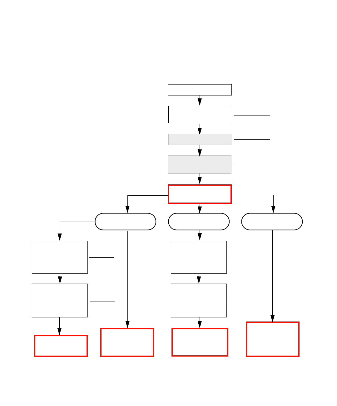
This diagram shows the activities involved in analyzing data with Varia workbench.
For more information about
each analysis, see Tab le 1- 1
on page 3.
Note: Preparation steps shown
in shaded boxes are optional and
only apply to some analysis
types.
Import genotype data
Filter for variations
in experiment
Deduce haplotypes
See page 5
See page 6
See page 13
Import pedigree,
link individuals
to genotypes, and
import traits
Mendelian Inheritance
check; remove SNPs
and individuals with
Mendelian errors
• TDT
• HHRR
See page 7
See page 8
• ANOVA
• Case Control
• Regression
Association
(
See page 14)
Generate populations
(allele frequencies)
Select type of analysis
Linkage
See page 22)
(
Import pedigree,
link individuals
to genotypes, and
import traits
Mendelian Inheritance
check; remove SNPs
and individuals with
Mendelian errors
• Parametric Linkage
• Single Point NPL
• Multipoint NPL
See page 10
Other analyses
See page 26)
(
See page 7
See page 8
• Find Autozygous
Regions
• Loss of
Heterozygosity
2 Varia Analysis Workbench Quick Start Guide
Page 3

Table 1-1 Types of Analyses in Varia Workbench
Analysis Type Pedigree? Description
Association Performed on larger outbred populations. (page 14)
ANOVA
(page 14)
Qualitative Case
Control (page 15)
Quantitative Case
Control (page 15)
Regression
(page 17)
Family-based
Association Analysis
(TDT and HHRR)
(page 19)
Linkage Performed on related groups of individuals. (page 22)
Parametric Linkage
(page 22)
Non-parametric
Linkage (NPL)
(page 24)
Other (page 26)
No Finds variations whose genotypes segregate individuals with respect to a quan-
titative trait. It is used when you have hundreds or thousands of unrelated individuals with high and low values of a quantitative trait.
No Estimates the linkage disequilibrium between two markers in a group of unre-
lated individuals with and without a particular phenotype.
No Estimates the linkage disequilibrium between two markers in a group of unre-
lated individuals with high and low values of a quantitative trait.
No Looks for association between genotypes and one or more phenotypes in a
large group of individuals (hundreds) when the non-genetic contributions to a
disease are thought to be important.
Yes Provides a complete set of linkage disequilibrium statistics that indicate the level
of association of a set of variations of interest to a specific trait or affliction
Requires a large number of individuals and pedigree data with known genotypes for both parents and their affected offspring.
Yes Estimates the recombination frequency between two markers when you have
genotyped many people in multiple generations in a pedigree.
Yes Localizes the genetic basis of a trait when you don’t have an exact model of the
genetics of the trait, but do know who is affected and unaffected by the disease
within a pedigree. A common example of NPL analysis is Affected Sibling Pair
analysis (ASP).
Find Autozygous
Regions
(page 26)
Loss of Heterozygosity (LOH)
(page 28)
No Finds homozygous regions in affected individuals that are likely to be inherited
from a common ancestor.
No Looks for statistically significant regions that are more homozygous in trans-
formed tissues than in pre-transformed tissues or in late-stage compared to
early-stage tumors.
Varia Analysis Workbench Quick Start Guide 3
Page 4
Starting Varia Workbench
1 Install Varia workbench according to the instructions given in the Varia Workbench
Installation Manual.
2 Double-click the Varia workbench icon on the desktop.
3 A Helpful Hint is displayed that tells you how to load data. Click OK to close the
Hint window.
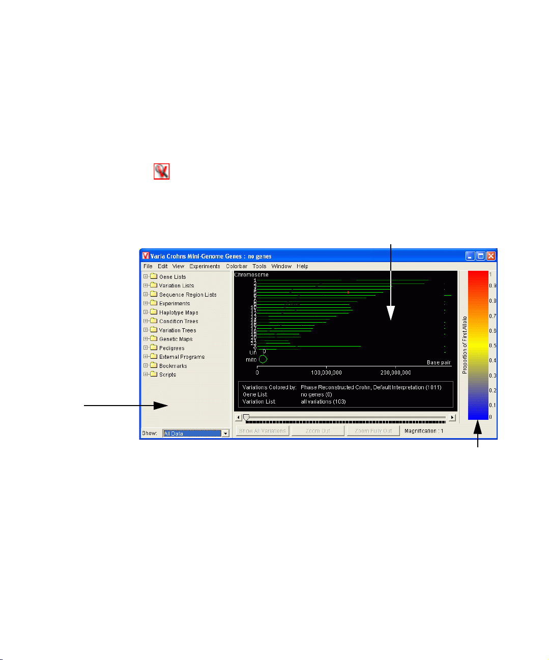
The Varia workbench main window appears.
Genome Browser
Navigator Pane
Colorbar
4 Proceed to “Import genotype data” on page 5.
Varia Workbench allows you to analyze data in many different ways. Often the
analyses are dictated by the data; how the study was conducted and whether or not
you have pedigree information for the individuals in the study.
4 Varia Analysis Workbench Quick Start Guide
Page 5

Preparing for Analysis
The following activities are prerequisites for some analyses in Varia workbench:
Import genotype data
(Applies to all analyses.)
1 Select Import Data from the File menu.
2 Select a text file that contains the genotype data and click the Open button.
3 Confirm the selection of the correct data file format and genome on the Import
Data: Define File Format and Genome window, then click the Next button. In most
cases the file format will be Affymetrix or Silicon Genetics Internal SNP.
Verify that the variations that you are studying are in the current genome build. If not,
add your variations to the existing genome prior to importing data by using the Edit
Master Table of Variations command on the Edit menu. See Chapter 16 in the
User’s Guide for more information.
4 Add additional samples for experiment if needed on the Selected Files window, and
click the Next button.
5 (optional) Add attributes on the Sample Attributes window. Add any additional
information on the individuals in your experiment that is usually in the pedigree file
such as gender.
Note The Individual ID is the combined information from family identifier and individual
identifier in the pedigree file separated by a period (.). For example, if the first
individual in the pedigree comes from family 66 and has the individual identifier 1,
the Individual ID will be 66.1. You can add this now or from the Experiment
Checklist in Step 9.
6 (optional) Add an attribute field such as Founder, if you intend to generate the allele
frequencies using only the founders or any individual from your samples. The
founder-only method is recommended if you have more than 50 founders from the
same population in your sample set (Ott, 1992). Mark every individual that is a
founder with an uppercase F in the appropriate field so that you can sort on it later.
7 To add other attributes, copy the information from your pedigree file and paste it into
the respective attribute column. Make sure that the rows in the file you’ve copied
match the Sample Attribute window.
8 When you have finished adding attributes, click the Next button. You are prompted to
Create Experiment. Click the Ye s button to generate the experiment.
Varia Analysis Workbench Quick Start Guide 5
Page 6

9 Name and save the experiment. Use the New Experiment Checklist to prepare your
data for analysis: Define Parameters, Define the Default Interpretation, and Link
Pedigree Individuals To Samples. It is also a good idea to assign a project to the
study at this point.
10 (optional) Modify attributes as described below.
Modify sample attributes
(Applies to all analyses.)
Use this procedure if you need to modify sample attributes.
1 Select Sample Manager from the Experiments menu.
2 Click the Filter on Experiment tab in the Sample Manager window.
3 Select your samples of interest in the Filter Results table.
4 Click the Add button. The samples appear in the Selected Samples table.
5 Click the Edit Attributes button to inspect, change, or add attributes. When you are
finished, click OK to close the Edit Attributes window.
6 Click OK to close the Sample Manager window.
Filter for variations in experiment
(Applies to all analyses.)
The Varia human genome contains millions of variations. Use the procedure below to
create a subset of these variations that contain data specific to your experiment.
1 Select Find Variations with Data in Experiment from the Tools menu.
2 In the Run Script window, select your experiment from the Experiments folder in
the Navigator pane and click the Experiment button in the Inputs area.
3 Click the Start button to run the script.
4Save the new variation list, and it will appear in the Variation Lists folder in the
Navigator pane of the Varia workbench main window.
5 (optional) Assign a project to the new variation list.
6 Varia Analysis Workbench Quick Start Guide
Page 7

Import pedigree
(Applies to Linkage analyses and Family-based Association analyses only.)
A pedigree describing individuals, their relationships, and affliction status is required to
perform family-based genetic analysis. Use the procedure below to import a
tab-delimited pedigree text file. After the pedigree has been imported, match individuals
in the pedigree to corresponding genotyped individuals and define the traits that are
associated with the pedigree.
1 Select Import New Pedigree from the File menu.
2 Select the pedigree text file that corresponds to your experiment, then click the Open
button.
3 You are prompted to provide the meaning of any extra columns (traits).
4 Name and save the pedigree. It is also a good idea to assign a project to the pedigree
at this point.
5 A Link Individuals to Samples window opens automatically. Fill it out now or click
Cancel to close the window if you don’t want to fill it out at this time.
Link individuals to samples
Family-based analyses use genotyped individuals who have been matched to pedigree
individuals. When a pedigree is imported, the link window is automatically active, but
you can also open the window to make changes as described below.
a Right-click on the pedigree in the Navigator pane and select Inspect from the
shortcut menu to display the Pedigree Inspector.
b Click the Link to Experiment button on the Individuals in Pedigree tab to
display the Link Individuals to Samples window.
c Link each person from your pedigree to the experimental data. Each person in the
pedigree is listed in the Individuals table. The persons in the experiment file are
listed in the Samples table. Persons in the Individuals table are automatically
linked with persons in the Samples table if the Individual ID and Sample ID
match. These pairs are listed in the Individual/Samples Pairs table on the right
side of the Link Individuals to Samples window.
Alternate
method
Varia Analysis Workbench Quick Start Guide 7
You can also add Individual IDs to samples by selecting Deduce Pedigree from the
Tools menu.
Page 8

Define traits
For some diseases, the inheritance model relating to a pedigree is known. The relevant
information such as phenotypes, penetrance, and allele frequencies can be defined for
these traits as described below.
a On the Trait Details tab of the Pedigree Inspector window, click the Add New
button.
b When the Edit Trait window opens, enter the values for the trait, define the
disease model, and add penetrance information.
c Click OK to close the Edit Trait window. The trait you just added appears in the
Trait Details tab of the Pedigree Inspector.
d Repeat Steps a-c for all traits you want to add.
Run Mendelian inheritance check
(Applies to Linkage analyses and Family-based Association analyses only.)
Prior to performing family-based parametric analyses, we recommend evaluating
variations for observance of Mendelian inheritance. This procedure will identify
genotyping errors.
1 Select Check Inheritance from the Tools menu.The Run Script window opens.
2 Select your experiment in the Navigator pane on the left side of the window, and
click the Genotypes button in the Inputs area.
3 Select the Vari a tio n Lis t for your experiment in the Navigator pane, and click the
To check button in the Inputs area. The variation list was created as described in
“Filter for variations in experiment” on page 6.
4 Select the Pedigree for your experiment in the Navigator pane, and click the
Pedigree button in the Inputs area.
5 Use the supplied default values for the following knobs, or enter different values if
you want:
• Allowable proportions of errors in %
• P value cutoff, to set what violates the inheritance rules
6 Click the Start button. The results are displayed in two tables; one that shows the
variations that seem to violate the inheritance rules and one that shows the
individuals that violate the inheritance rules.
7 Investigate the variations in the two lists. If necessary, variations or individuals with
unusually high genotyping errors can be removed as described below.
8 Varia Analysis Workbench Quick Start Guide
Page 9

Remove individuals with Mendelian errors
Use this procedure after running the Mendelian inheritance check described on page 8.
a (optional) Make a copy of your existing pedigree as follows:
• Display the pedigree in Pedigree Diagram view in the Genome Browser pane of
the Varia workbench window.
• Select all the individuals in the pedigree, right-click in the Browser pane, and
select Make Pedigree from Selected Individuals from the shortcut menu.
• Name and save the copy of the pedigree.
b Using the Check-Inheritance Results table as a guide, remove the trios that have
inheritance errors as follows:
• Select the individuals in the Browser pane
• Right-click and select Delete Selected Individuals from the shortcut menu.
Note
If the parents have another child that does not show inheritance errors, then only remove
the child that shows errors, rather then the child and both parents.
c (optional) Re-run the Mendelian inheritance test to see if the variation list
changes.
Remove SNPs with Mendelian errors
Use this procedure after running the Mendelian inheritance check described on page 8.
a Select Physical Position from the View menu.
b Right-click on the variation list that contains the inheritance errors in Navigator,
and select Venn Diagram > Left from the shortcut menu.
c Right-click on the complete variation list for your experiment in Navigator (i.e.
the one that includes Mendelian errors), and select Venn Diagram > Right from
the shortcut menu.
d Select the complete variation list for your experiment again and set as Universe
using the Venn diagram option. Inspect the Venn diagram on the right side and
make sure the lists are correct.
e Right-click on the non-overlapping region in the complete variation list (the
green segment), and select Make list of variations in this list only from the
shortcut menu. The new variation list will contain only variations without
Mendelian errors.
Varia Analysis Workbench Quick Start Guide 9
Page 10

Generate populations to establish allele frequencies
(Applies to some types of Linkage analyses and Autozygosity analyses.)
You can generate populations to establish allele frequencies in the following ways:
• Use your own samples (founders only) (page 10)
• Use Affymetrix frequencies (page 11)
• Import your own allele frequencies (page 11)
Use your own samples (founders only)
The following procedure allows you to generate a population containing allele
frequencies using individuals from your experiments.
1 Select Sample Manager from the Experiments menu.
a Click the Filter on Experiment tab, select the experiment of choice.
b Sort on attributes (e.g. Founders) in the Filter Results table.
c Click on each individual in the Filter Results table that you want to use to
generate allele frequencies. Click the Add button to add the samples to the
Selected Samples table. At least 50 founders should be selected.
d Click the Create Experiment button to create an experiment that contains the
individuals in the Selected Samples table.
2 Right-click on the sample file in the Experiment folder in the Navigator pane and
select Inspect from the shortcut menu.
a Click the Interpretation tab in the Experiment Inspector window.
b Click on Default Interpretation and select Do not Display.
c Save this file as a new interpretation (e.g. population condition). This results in a
single averaged condition with that interpretation.
3 Run the following script from the Basic Scripts folder of Navigator:
Merge-Split Groups > Merge Condition to Sample
a Select the single averaged condition that you generated in Step 2 from the
Experiment folder, and click the Condition button in the Inputs area.
b Leave the Data compression method as Population.
c Click the Start button to run the script. A new sample containing population allele
frequencies is created and displayed in a Sample Inspector window.
d Name and save the sample. It is also a good idea to assign a project to the sample
at this point. This sample is now available in the Sample Manager window.
10 Varia Analysis Workbench Quick Start Guide
Page 11

4 (optional) Open the Sample Manager window from the Experiments menu.
a Sort the samples by date.
b Add the new population sample to the sample list.
c Create an experiment from this new sample.
Use Affymetrix frequencies
Affymetrix provides allele frequencies for their SNPs from African-American, Asian
and Caucasian populations. Contact Affymetrix for additional information.
1 Drag the Affymetrix Population Fre.zip file into the Varia workbench window, or
select Import Varia Zip from the File menu in the main window. Contact Agilent
Technical support for information on how to get this file if you don’t have it.
2 You can select these population files in the Experiments folder in the Navigator
pane.
Import your own allele frequencies
1 To import your own population frequencies, create an allele frequency file with the
following format. This is one of several input file formats supported in the Varia
Workbench.
# SiGSNP2.0 (Version)
# type=3 (Type of data: 3=population)
# chroms=2 (number of Chromosomes in organism)
# samples=1 (number of samples: 1 for populations)
# name=Population (identity of population)
rs1376173 A:0.2,G:0.8 (SNPID Allele1:Frequency1,Allele2:Frequency2)
rs1254601 C:0.2,T:0.8 (SNPID Allele1:Frequency1,Allele2:Frequency2)
rs1254600 C:0.8,T:0.2 (SNPID Allele1:Frequency1,Allele2:Frequency2)
Varia Analysis Workbench Quick Start Guide 11
Page 12

2 Select Import Data from the File menu.
a Select the genome, such as Homo Sapiens build 34v2 db SNP.txt, and click the
Open button.
b Click the Next button on the Define File Format and Genome window.
c Add additional samples for experiment if needed on the Selected Files window,
and click the Next button.
d Click the Next button on the Sample Attributes window.
e You are prompted to Create Experiment. Click the Yes button to generate the
experiment.
fSave the experiment.
12 Varia Analysis Workbench Quick Start Guide
Page 13

Deduce haplotypes
(Applies to Linkage analyses and Family-based Association analyses only.)
Individual variations can be organized as haplotype blocks. The data may be analyzed
by variations or haplotype blocks formed by adjacent variations that exhibit linkage. Use
the following procedure to generate haplotypes from an experiment if you have pedigree
data.
Note
Before you start This tool requires that samples have an "Individual ID" attribute. Manually add unique
If you don’t have pedigree data, use the script QC & Analysis > Haplotypes > Deduce
Haplotypes (No Pedigree) in the Basic Scripts folder.
entries in the "Individual ID" attribute field on the Edit Attributes window, which you
can access from the Sample Manager window. Any samples that do not have an
"Individual ID" attribute will not be included in the resulting pedigree.
1 Select Deduce Haplotypes from the Too ls menu.
2 In the Run Script window, select your experiment from the Experiments folder in
the Navigator pane, then click the Experiment button.
3 Select the variation list that corresponds to your experiment from the Va r ia t i on L i st
folder in the Navigator pane, then click the Va r iat i o n L i s t button.
4 Select the pedigree for your experiment from the Pedigree folder in the Navigator
pane, then click the Pedigree button.
5 Accept the defaults provided or enter different values for the following inputs:
• Error rate
• Algorithm
• New Call Confidence
6 Click the Start button.
7 You are prompted to create an experiment of the haplotyped samples. Click Ye s to
create an experiment with the samples that contain the computed haplotypes
(Haplotype blocks) expression in each (phase-known) individual.
8 Name and save the haplotype experiment and project, if you are using one.
Note
Varia Analysis Workbench Quick Start Guide 13
If you had defined interpretations in the original non-haplotyped experiment, you will
have to redefine them in the haplotyped experiment.
If you have complete family information, the result is a comprehensive list of phase
known haplotypes that you can use for Linkage analysis or Family-based association
studies (TDT or HHRR).
Page 14

Association Analyses
Association analyses are performed on larger outbred populations and include the
following:
• ANOVA (page 14)
• Case Control (page 15)
• Regression (page 17)
Family-based Association tests (TDT and HHRR) are described on (page 19).
ANOVA
ANOVA (Analysis of Variance) is used to find variations whose genotypes segregate
individuals with respect to a quantitative trait. It is used when you have hundreds or
thousands of unrelated individuals with high and low values of a quantitative trait.
1 Prepare for ANOVA analysis with the following steps:
a “Import genotype data” on page 5
b “Filter for variations in experiment” on page 6
2 Select Association > ANOVA from the Tools menu.
3 In the ANOVA window, select one of the following options for Estimate the
association between a trait and:
• Trait
• Va ri a ti o n
• Var ia ti on Li st
• Haplotype Block
• List of Haplotype Blocks
4 (Variation or Haplotype block only) Click the Find button to open the Choose
Var ia ti on window, and select the variation of interest.
5 (Variation List or List of Haplotype Blocks only) Select the variation list that
corresponds to your experiment from the Va r i at i o n L i s t folder in the Navigator
pane, then click the Choose Variation List button.
6 Select your experiment from the Experiments folder in the Navigator pane, then
click the Choose Experiment button.
7 (Haplotype Block or List of Haplotype Blocks only) Select a haplotype map from the
Haplotype Maps folder in the Navigator pane, then click the Choose Haplotype
Map button.
8 Select the Quantitative Trait of interest from the list.
14 Varia Analysis Workbench Quick Start Guide
Page 15

9 Select one of the following types for Genetic Variable:
• Allele Count - Divides the samples into groups based on the alleles of the marker
• Genotype - Divides the samples into groups based on genotypes of the marker
10 Accept the defaults provided for the Low and High Trait Cutoff values or enter
different values.
11 Click the Start button to run the analysis.
12 The results are a statistic for the Trait, Variation and Haplotype Block analysis types
and a variation list for the Variation List and List of Haplotype Blocks analysis types.
You can save the variation list or copy the table to the Clipboard and paste into Excel.
Case Control
The case control algorithms in Varia workbench are designed to look for measured
genotypes that are found more frequently in diseased individuals (cases) than they are in
non-diseased individuals (controls). Perform case-control analysis as follows:
1 Prepare for case-control analysis with the following steps:
a “Import genotype data” on page 5
b “Filter for variations in experiment” on page 6
c (optional) “Deduce haplotypes” on page 13
d Check ethnicity to avoid problems with admixture by running the Personal
2 Select Association > Qualitative Case Control or Association > Quantitative Case
Control from the Too ls menu, depending on whether the trait you are studying is
qualitative or quantitative.
3 In the Case-Control window, select the two types of measurements that you want to
test for association. These can include almost any combination of the following:
• Traits
• Va ri a ti o n s
• Var ia ti on Li st s
• Haplotype Blocks
• Lists of Haplotype Blocks
locus.
locus.
Genetics > Genetic Admixture script in the Basic Scripts folder in Navigator.
See the Testing for Association section of the Varia Analysis Workbench User’s
Guide for more information.
Varia Analysis Workbench Quick Start Guide 15
Page 16

For Quantitative Case Control, you select one of the above measurement types to
compare to the quantitative trait you select.
4 (Variation or Haplotype block only) If you select an individual variation (rather than
a list) or an individual haplotype block, look up the identifier for that locus. Click the
Find button to open the Choose Variation window, and select the variation of
interest. Note that this option is only available if you have selected a single locus
measurement type in Step 3.
5 (Quantitative case-control only) Once you define the quantitative trait, you will see a
histogram that shows the distribution of values in your experiment. In some studies,
statistical power is gained by excluding individuals with mid-level values from the
analysis and only using individuals with extreme values of the given trait. Use the
diamond-shaped sliders to specify the samples to be used in your experiment, and to
identify where the thresholds for high and low values begin. Any samples (values)
with a lavender bar beneath them will be included in the experiment.
6 Click the Start button to run the analysis.
7 Review and save the analysis results. See the Varia Analysis Workbench User’s Guide
for more information.
a One of the best ways to see if you have an interesting result is to sort the table
based on an interesting statistic, such as the Chi Squared value. Then look at the
Physical Position column. If the highest chi squared values are all within a narrow
region of the genome, this is an interesting result.
b Another way to rationalize the results of a case-control analysis is to plot any of
the statistics from the resulting variation table in the Physical Position view in the
Browser pane. Look for regions with consistently high association scores (or low
p-values). If neighboring variations exhibit high association scores, this also
indicates that you have found an interesting region.
16 Varia Analysis Workbench Quick Start Guide
Page 17

Regression
Regression analysis is used to identify the contribution of one or more genetic or
non-genetic markers to the disease phenotype (dependent variable). This is especially
powerful when the non-genetic markers are thought to be influential in their contribution
to the disease or are thought to alter the measurement of the disease phenotype. Perform
regression analysis as follows:.
1 Prepare for regression analysis with the following steps:
2 Select Association > Regression (One Model) or Association > Regression (Many
3 In the Regression window, select one of the following options to Estimate the
a “Import genotype data” on page 5
b “Filter for variations in experiment” on page 6
c (optional) “Deduce haplotypes” on page 13
d “Generate populations to establish allele frequencies” on page 10
e Check ethnicity to avoid problems with admixture by running the Personal
Genetics > Genetic Admixture script in the Basic Scripts folder in Navigator.
See the Testing for Association section of the Varia Analysis Workbench User’s
Guide for more information.
Models) from the Tools menu, depending on the type of Regression analysis you
want to perform.
• One Model - This mode performs a single regression that can contain any number
of genetic or non-genetic covariates.
• Many Models - This mode performs a separate regression (model) for each entry
in a list of variations. Each regression is different from the others in that a different
independent variable is selected from the variation list. The many models
regression can also include any number of genetic or non genetic covariates that
are identical for each regression.
association between a trait and a:
• Trait
• Va ri a ti o n
• Variation List - Note that in the "one model" option, many variation lists are so
large that it is unsuitable to include each variation as an independent variable in a
single regression.
• Haplotype Block
• List of Haplotype Blocks - Note that in the "one model" option, many variation
lists (representing haplotype blocks) are so large that it is unsuitable to include
each block as an independent variable in a single regression.
Varia Analysis Workbench Quick Start Guide 17
Page 18

4 (Variation or Haplotype block only) Click the Find button to open the Choose
Var ia ti on window, and select the variation of interest.
5 (Variation List or List of Haplotype Blocks only) Select the variation list that
corresponds to your experiment from the Va r i at i o n L i s t folder in the Navigator
pane, then click the Choose Variation List button. Note that in the “many model
modes” and especially in the “single model” modes, there is a significant statistical
penalty for selecting a list that is too long. In general, your results are more likely to
be meaningful if you shorten the input list using other criteria (biological or
statistical).
6 Select your experiment from the Experiments folder in the Navigator pane, then
click the Choose Experiment button.
7 (Haplotype Block or List of Haplotype Blocks only) Select a haplotype map from the
Haplotype Maps folder in the Navigator pane, then click the Choose Haplotype
Map button.
8 Select the Dependent Trait of interest from the list.
9 Click the Choose Variables button to open the Choose Independent Variables
window, and select the independent variables to use in the Regression Analysis.
These are the non-genetic (or non-dependent) traits that contribute to the disease.
10 Select one of the following types for Genetic Variable, which defines the manner in
which the genotypes for the Genetic Variable are encoded.
• Allele Count - This option includes a single independent variable for each of the
possible alleles of the Genetic Variable. For diploid samples, this will always be 0,
1, or 2. This option assumes that the effect of the disease allele is additive.
• Genotype - This option includes a set of Boolean variables for (one less than)
each of the possible permutations of two alleles. This option assumes that only
specific pairs of alleles are associated with the dependent variable.
11 (Quantitative traits only) Accept the defaults provided for the Low and High Sample
Cutoff values or enter different values to select the samples to use in the analysis,
from the samples already selected in the experiment. You can select samples on the
extreme ends of the phenotype, under the assumption that the more extreme the
phenotype, the more likely it is to be genetic. Samples are selected by entering values
in the High and Low Cutoff fields or by moving the sliders on the graph. Only
samples with quantitative trait values greater than or equal to the high cutoff or less
than or equal to the low cutoff are used.
12 Click the Start button to run the analysis.
The results are statistics for the Trait, Variation and Haplotype Block analysis types
and variation lists for the Variation List and List of Haplotype Blocks analysis types.
13 You can save the variation list or copy the table to the Clipboard and paste into Excel.
18 Varia Analysis Workbench Quick Start Guide
Page 19

Family-based Association (TDT and HHRR)
Varia workbench provides two algorithms for performing family-based association
analysis: Transmission/Disequilibrium Test (TDT) and Haplotype-based Haplotype
Relative Risk Test (HHRR). These tests are alternative methods of analysis compared to
case-control experiments. Both case-control and TDT/HHRR analyses are used to
elucidate linkage disequilibrium between an observable trait and a set of variations of
interest.
To increase the reliability of the analysis, TDT and HHRR are typically applied to
genotype data from at least hundreds of nuclear families with affected children. The
analysis requires a large number of individuals and pedigree data with known genotypes
for both parents and their affected offspring. The results provide the complete set of
linkage disequilibrium statistics that indicate the level of association of a set of
variations of interest to a specific trait or affliction.
TDT
Unlike case-control analysis, TDT overcomes the issue of population stratification, a
confounding factor resulting from the use of genetically distinct subsets for cases and
controls. As a result of population stratification, case-control analysis may reveal
significant disequilibrium that result from the inherent difference between the groups,
instead of revealing disequilibrium between an affliction and a variation. In TDT, the
controls are the parents of affected children. Because of the genetic similarity, controls
are appropriately matched to the cases. TDT is also specifically capable to detecting
disequilibrium due to linkage.
HHRR
While HHRR is not robust to population stratification, it is an analysis method that is
capable of using both homozygous and heterozygous parents, compared to TDT which
only includes parents with heterozygous genotypes. HHRR establishes significance of
disequilibrium by comparing transmitted to untransmitted alleles to affected individuals.
Perform family-based association analysis as follows:
Varia Analysis Workbench Quick Start Guide 19
Page 20

1 Prepare for TDT/HHRR analysis with the following steps:
a “Import data and create an experiment” on page 50.
b “Filter for variations in experiment” on page 56.
c (optional) “Deduce haplotypes with pedigree data” on page 72.
d (HHRR only) “Check Hardy-Weinberg equilibrium” on page 56.
e “Import pedigree data” on page 62.
f “Link pedigree individuals to samples” on page 64.
g “Define diseases and disease liability” on page 67.
h “Perform quality control check on pedigree data” on page 65.
i “Remove individuals with Mendelian errors” on page 66.
j “Remove SNPs with Mendelian errors” on page 66.
2 Select Association > Transmission Disequilibrium Test (TDT) from the To ols
menu.
3 In the Transmission Disequilibrium Test window, select one of the following
options to Estimate the association between a trait and a:
• Va ri a ti o n
• Var ia ti on Li st
• Haplotype Block
• List of Haplotype Blocks
4 (Variation or Haplotype block only) Enter the identifier of the variation of interest or
the variation that corresponds to a haplotype block of interest. If necessary, click the
Find button to perform a variation search on the Choose Variation window.
5 (Variation List or List of Haplotype Blocks only) Select the variation list that
corresponds to your experiment from the Variation List folder in the Navigator pane,
then click the Choose Variation List button.
6 Select your experiment from the Experiments folder in the Navigator pane, then
click the Choose Experiment button.
Specify a haplotype reconstructed experiment if you selected Haplotype Block or
List of Haplotype Blocks in Step 3. You can create this experiment by selecting
Deduce Haplotypes from the Tools menu or by selecting Create New Experiment
from the Experiments menu.
7 (Haplotype Block or List of Haplotype Blocks only) Select a haplotype map from the
Haplotype Maps folder in the Navigator pane, then click the Choose Haplotype
Map button.
20 Varia Analysis Workbench Quick Start Guide
Page 21

8 Select the pedigree for your experiment from the Pedigree folder in the Navigator
pane, then click the Choose Pedigree button.
9 Select the Trait of interest from the list.
10 Select TDT or HHRR as the Tes t Typ e , depending on which analysis you want to
run.
11 Click the Start button to run the analysis.
12 Review and save the analysis results.
For TDT, Chi squared, Degrees of Freedom, and P-value statistics are calculated.
For HHRR, D, D', Rho, Chi squared, Degrees of Freedom, P-value, and T to U ratio
statistics are calculated. T to U is the ratio of the number of times the most highly
transmitted allele is transmitted to the number of times it is not transmitted.
See the Varia Analysis Workbench User’s Guide for more information.
13 You can obtain a visually informative representation of the data by plotting each
disequilibrium statistic from a resulting variation table list in the Physical Position
view in the Browser pane. Typically you want to look for regions with consistently
high association scores (or low p-values). If neighboring variations exhibit high
association scores, this is also an indication that you have found an interesting region.
Varia Analysis Workbench Quick Start Guide 21
Page 22

Linkage Analyses
Linkage analyses are performed on related groups of individuals and require pedigree
information and include the following analysis options:
• Parametric Linkage (page 22)
• Non-parametric Linkage (NPL) (page 24)
Parametric Linkage
Parametric linkage analysis is used to estimate the recombination frequency between
two markers when you have genotyped many people in multiple generations in a
pedigree.
1 Prepare for Parametric Linkage analysis with the following steps:
a “Import genotype data” on page 5.
b “Filter for variations in experiment” on page 6.
c (optional) Deduce haplotypes as described in “Deduce haplotypes” on page 13.
d “Generate populations to establish allele frequencies” on page 10.
e “Import pedigree” on page 7, including linking individuals to genotypes, and
f “Run Mendelian inheritance check” on page 8, including removing SNPs and
2 Select Linkage > Parametric Linkage from the Tools menu.
3 In the Parametric Linkage window, select Estimate the linkage between Variation
List and Trait.
4 Select the variation list that corresponds to your experiment from the Va r ia t i on L i st
folder in the Navigator pane, then click the Choose Variation List button.
5 Select your experiment from the Experiments folder in the Navigator pane, then
click the Choose Experiment button.
6 Select the pedigree for your experiment from the Pedigree folder in the Navigator
pane, then click the Choose Pedigree button.
importing traits.
individuals with Mendelian errors.
22 Varia Analysis Workbench Quick Start Guide
Page 23

7 Click the Choose Population Sample button to display the Select Population
window.
a Select the Filter on Experiment tab, then sort the Filter Results table by
double-clicking the Type column heading.
b Click on the population sample in the Filter Results table that contains the allele
frequencies generated as described in “Generate populations to establish allele
frequencies” on page 10.
c Click the Add button to add it to the Selected Samples table.
d Click OK to close the Select Population window.
8 Select the Trait of interest from the list.
9 Accept the defaults provided or enter different values for the following inputs:
• Theta Values
• Number of Consecutive Variations to Combine
10 Click the Start button to run the analysis.
Note
The computation can take more than eight hours, depending on the size of your
pedigree.
11 When the results are displayed, you can save the resulting table as a variation list or
copy the table to the Clipboard and paste into Excel.
Varia Analysis Workbench Quick Start Guide 23
Page 24

Non-parametric Linkage (NPL)
NPL analysis is used to localize the genetic basis of a trait when you don’t have an exact
model of the genetics of the trait, but do know who is affected and unaffected by the
disease within a pedigree. A common example of NPL analysis is Affected Sibling Pair
analysis (ASP).
1 Prepare for NPL analysis with the following steps:
a “Import genotype data” on page 5.
b “Filter for variations in experiment” on page 6.
c (optional) Deduce haplotypes as described in “Deduce haplotypes” on page 13.
This step is important for Multipoint NPL analysis, which assumes that the
variations used in the analysis are unrelated to each other, i.e. that they are not in
linkage disequilibrium. The resulting LOD scores can be artificially inflated if
multiple variations from a region with high LD (or "hot zone") are included. In
particular, the variation list should be streamlined for Multipoint NPL analysis
when using high density chips, so that only one variation represents a region with
high LD.
d “Generate populations to establish allele frequencies” on page 10.
e “Import pedigree” on page 7, including linking individuals to genotypes, and
importing traits.
f “Run Mendelian inheritance check” on page 8, including removing SNPs and
individuals with Mendelian errors.
2 Select Linkage > Non Parametric Linkage (NPL) from the Tools menu.
3 In the NPL window, select Estimate the association between a trait and a
Vari a tio n Lis t .
4 Select the Single or Multiple Point Linkage option.
5 Select the variation list that corresponds to your experiment from the Va r ia t i on L i st
folder in the Navigator pane, then click the Choose Variation List button.
6 Select your experiment from the Experiments folder in the Navigator pane, then
click the Choose Experiment button.
7 Select the pedigree for your experiment from the Pedigree folder in the Navigator
pane, then click the Choose Pedigree button.
24 Varia Analysis Workbench Quick Start Guide
Page 25

8 Click the Choose Population Sample button to display the Select Population
window.
a Select the Filter on Experiment tab, then sort the Filter Results table by
double-clicking the Type column heading.
b Click on the population sample in the Filter Results table that contains the allele
frequencies generated as described in “Generate populations to establish allele
frequencies” on page 10.
c Click the Add button to add it to the Selected Samples table.
d Click OK to close the Select Population window.
9 Select the Trait of interest from the list.
10 Accept the defaults provided or enter different values for the following inputs:
Single Point Linkage Inputs Multiple Point Linkage Inputs
• Statistic • Statistic
Note
• Maximum number of bits for the
inheritance vector
• Number of Consecutive Variations to
Combine
• Mapping Function
• Error Rate
• Maximum number of bits for the
inheritance vector
• Include results between variations
11 Click the Start button to run the analysis.
The computation can take more than eight hours, depending on the size of your
pedigree.
12 When the results are displayed, you can save the resulting table as a variation list or
copy the table to the Clipboard and paste into Excel.
Varia Analysis Workbench Quick Start Guide 25
Page 26

Other Analyses
In addition to the Linkage and Association analyses described previously, the following
additional analyses are available in Varia workbench:
• Find Autozygous Regions (page 26)
• Loss of Heterozygosity (page 28)
Find Autozygous Regions
This analysis finds homozygous regions in affected individuals that are likely to be
inherited from a common ancestor. In an inbred population that is enriched in
individuals with rare recessive diseases, this approach can be very powerful in
identifying regions that span the disease locus. Find autozygous regions as follows:
1 Prepare for to find autozygous regions with the following steps:
2 Select Find Autozygous Regions from the Tools menu.
3 In the Find Autozygous Regions window, select one of the following combinations
4 Select the variation list that corresponds to your experiment (or to the variations from
5 (Families only) Select your experiment from the Experiments folder in the
a “Import genotype data” on page 5
b “Filter for variations in experiment” on page 6
for the analysis:
• Individual / Haplotype Map - This option requires a haplotype map for the
population that best fits the individual.
• Individual / Population - This option requires the use of a population sample that
describes the allele frequencies of the measured loci. If you do not have a
population sample, you can select multiple samples from individuals who you
believe are genetically (ethnically) similar to the individual in question.
• Families / Haplotype Map - This option requires a haplotype map for the
population that best fits the individual.
• Families / Population - This option requires the use of a population sample that
describes the allele frequencies of the measured loci. If you do not have a
population sample, you can select multiple samples from individuals who you
believe are genetically (ethnically) similar to the individual in question.
your experiment that have passed relevant quality control tests) from the Va ri at i on
List folder in the Navigator pane, then click the Choose Variation List button.
Navigator pane, then click the Experiment button.
26 Varia Analysis Workbench Quick Start Guide
Page 27

6 (Haplotype Map only) Select a haplotype map from the Haplotype Maps folder in
the Navigator pane, then click the Haplotype Map button.
7 (Families only) Select the pedigree for your experiment from the Pedigree folder in
the Navigator pane, then click the Pedigree button.
8 (Individual only) Click the Choose Individual Sample button to display the Select
Individual Sample window.
a Select the appropriate filtering method, then click on the sample of interest in the
Filter Results table.
b Click OK to close the Select Individual Sample window.
9 (Population only) Click the Choose Population Sample button to display the Select
Population window.
a Select the Filter on Experiment tab, then sort the Filter Results table by
double-clicking the Type column heading.
a Click on the population sample of interest in the Filter Results table.
b Click the Add button to add it to the Selected Samples table.
c Click OK to close the Select Population window.
10 (Families only) Select the Recessive Trait of interest from the list.
11 Accept the defaults provided or enter different values for the following inputs:
• Error Rate - The estimated error rate for the genotyping measurement technology.
Consult your hardware vendor for good estimates.
• LOD Score Cutoff - The cutoff of the regional LOD score that is used to build
sequence region lists. Segments of sequence with regional LOD scores above the
threshold are included in the sequence region lists.
12 Click the Start button to run the analysis.
13 When the results are displayed, you can save the resulting table as a variation list or
copy the table to the Clipboard and paste into Excel. The analysis also produces a
homozygous sequence regions list, which may be saved or copied to the Clipboard.
Varia Analysis Workbench Quick Start Guide 27
Page 28

Loss of Heterozygosity
LOH analysis looks for statistically significant regions that are more homozygous in
transformed tissues than in pre-transformed tissues or in late-stage compared to
early-stage tumors. Varia workbench allows you to perform LOH studies on groups of
tumor/nontumor pairs or on single tumors using a common non-tumor reference. Several
summarization methods are available to characterize the most common regions that
suffered replication defects. The algorithm is very similar to the one used to detect
autozygosity in inbred populations. To use this tool, you need to have pairs of
transformed and pre-transformed samples, presumably from the same individuals. You
can pair the related samples in either of the following ways:
• If you have used sample attributes to designate individuals and tumor state, select the
Pair By Attributes option.
• To manually assign the pairs, select the Assign Custom Pairs option.
If you have designed your experiment so that instead of sample pairs, you have tumor
samples from a number of individuals and a single reference sample representing
healthy tissue, you can still use the LOH tool in Varia workbench to analyze the
experiment.
Perform the loss of heterozygosity analysis as follows:
1 Prepare for LOH analysis with the following steps:
a “Import genotype data” on page 5
b “Filter for variations in experiment” on page 6
2 Select Loss of Heterozygosity from the Tools menu.
3 In the Loss of Heterozygosity window, select the variation list that corresponds to
your experiment from the Va r iat i on L i st folder in the Navigator pane, then click the
Choose Variation List button.
4 Select your experiment from the Experiments folder in the Navigator pane, then
click the Choose Experiment button. Optionally, you can use the Add/REmove
Samples button add samples or to exclude samples from the experiment.
5 Accept the defaults provided or enter different values for the following inputs:
• Error Rate - the estimated error rate resulting from the genotyping measurement
technology
• LOD Score Cutoff - - the threshold for the log of odds ratio beyond which a region
of variations is considered to have significant loss of heterozygosity
• Minimum Individuals - the fewest number of individuals that must exhibit LOH
for a region to be included in the analysis
28 Varia Analysis Workbench Quick Start Guide
Page 29

6 Pair the pre-transformed and transformed samples either manually (custom pairs) or
automatically by attributes. If you select the Assign Custom Pairs option, a separate
window appears when you click OK, which allows you to create the desired pairs of
samples (see Step 8).
7 (optional) If you select the Pair By Attributes option, click the Preview button to
see the pairs of Pre-Transformed and Transformed samples that will be used in the
analysis. Errors found in any of the samples are displayed at the bottom of the
Preview window.
8 Click the Start button to run the analysis.
If you selected the Assign Custom Pairs option in Step 6, the Custom Pairs window
appears. Select samples from the Pre-Transformed and Transformed lists and click
the Add Pair>> button. The pairs appear in the table on the right side of the window,
which is the list of sample pairs that will be used for the analysis. Click OK on the
Custom Pairs window to start the LOH analysis.
9 When the results are displayed, you can save the resulting table as a variation list or
copy the table to the Clipboard and paste into Excel. The analysis also produces a
sequence regions list, which may be saved or copied to the Clipboard.
Varia Analysis Workbench Quick Start Guide 29
Page 30

What To Do Next
After running the analyses described in the preceding pages, you can use the following
procedures to further review the results.
Zoom into regions with high probability of linkage
Use the following procedure when you have a variation list that shows only variations
with a high probability of linkage (usually the output from an analysis), and you want to
scan for peaks using their associated numbers.
1 Zoom in on a variation in the Browser. A graph that shows the associated number,
usually an LOD score or P-value, is shown below the variation.
2 Pan the screen right or left with the arrow keys to look at other variations (and their
associated graphs) along the chromosome.
Visualize annotated genes
1 Select the genes in the Genome Browser in one of the following ways:
Single gene Click on any line or rectangle representing a gene in the Genome
Browser. The name of the selected gene appears in the legend at the bottom of the
Genome Browser.
Multiple genes Click on any line or rectangle representing a gene in the Genome
Browser, then <Shift>-click to select additional genes.
Alternate method <Shift>-click-and-drag across the genes you want to select. A box
appears as you drag. When you release the mouse, the selected genes are highlighted
(selected).
2 Right-click and select Make gene list from selected genes from the shortcut menu.
3 (optional) Select Save Image > Browser from the File menu. This opens the Export
Options window, which allows you to save the image as a PICT or PNG file for use
with other applications.
30 Varia Analysis Workbench Quick Start Guide
Page 31

Menu Commands in Varia Workbench
File Edit View Experiments Colorbar Tools
Import Data
Open
Genome or
Array
View
Projects
New Window
New Linked
Window
New Pedigree
Import New
Pedigree
Import Varia
Zip
Save Bookmark
Print Image
Save Image
Close
Quit
Copy
>Variation List
>Gene List
Paste
>Variation List
>Gene List
Undo
Find Variation
Find Next Variation
Advanced Find
Var iati on
Inspect
Selected Variation
Find Gene
Find Next Gene
Advanced Find
Gene
Inspect
Selected Gene
Find Individual
Search
Filter Navigator
Standard
Attributes
Edit Master
Table of Variations
Preferences
Physical
Position
Tree
Graph
Bar Graph
Scatter Plot
3D Scatter
Plot
Linkage Disequilibrium
(GOLD) Plot
Pedigree
Diagram
Spreadsheet
Zoom In
Zoom Out
Zoom Fully
Out
Visible
Display
Options
Experiment
Inspector
Experiment
Parameters
Experiment
Interpretation
Create New
Experiment
Duplicate
Experiment
Sample Manager
Color by:
Proportion of
First Allele
Proportion Minus
Mean
Proportion
Divided by Mean
Estimated Heterozygosity
Heterozygosity
Divided by Mean
T-Score of First
Allele
T-Test P -Value
Chi Squared
Score
Chi Squared
P-Value
Cramer’s V
Parameter
Venn Diagram
No Color
Find Variations with Data in
Experiment
Deduce Pedigree
Check Inheritance
Check Hardy-Weinburg
Equilibrium
Deduce Haplotypes
Linkage
>Parametric
>Non-Parametric
Association
>ANOVA
>Qualitative Case-Control
>Quantitative Case-Control
>Regression (One Model)
>Regression (Many Models)
>Transmission Disequilibrium Test (TDT)
More Variation Tools
Find Autozygous Regions
Loss of Heterozygosity
Find Potential Regulatory
Sequences
Create Variation Table
Script Editor
See the Varia Analysis Workbench User’s Guide for a description of commands that
appear on the
Window and Help menus.
Varia Analysis Workbench Quick Start Guide 31
Page 32

Tips for Viewing Data in the Genome Browser
To change the display of data
Mouse Action or Key Stroke Result Menu Command
Drag a rectangle across a region that you want
to expand. Repeat the process until you reach
the desired magnification level.
Click the Zoom Out button at the bottom of the
Genome Browser or right-click and select
Zoom Out.
Click the Zoom Fully Out button at the bottom
of the Genome Browser or right-click and
select Zoom Fully Out.
Left arrow, Right arrow Pans horizontally None
Up arrow, Down arrow Pans vertically None
PageUp, PageDown Pans vertically by
To change the Genome Browser view
Select one of the following commands from the View menu in the Varia workbench
window:
• Physical Position • Scatter Plot
• Tree • 3D Scatter Plot
• Graph • Linkage Disequilibrium (GOLD Plot)
Zooms in
(expands selected
region)
Zooms out one
level
Zooms out completely
a whole screen
View > Zoom In
View > Zoom Out
View > Zoom Fully Out
None
• Bar Graph • Pedigree Diagram
Note that the Browser view changes automatically when you select certain data objects
in the Navigator. For example, when you select a pedigree object, the Browser view
automatically changes to Pedigree Diagram view.
32 Varia Analysis Workbench Quick Start Guide
Page 33

To access Browser shortcut menu commands
Right-click in the Browser pane to access the following commands:
Menu Command Result
Zoom Out Decreases the detail shown in the view
Zoom Fully Out Returns the view to the original data display
To select variations and genes
Single variation
or gene selection
Make List from Selected
Variations
Make List from Selected
Genes
Inspect Selected Variations Pans vertically
Save Image Allows you to save the image of the Genome Browser in either a
Save Bookmark Opens the Save New Bookmark Window. Bookmarks allow you
Delete Sequence Region
Element
Display Options Opens the Display Options window, which allows you to modify
Allows you to create a variation list from the selected variations
Allows you to create a gene list from the selected genes.
PNG or PICT file format
save your current display settings, including experiments, gene
list, coloration, and selected genes. The saved bookmark
appears in the Bookmarks folder in the Navigator pane, so that
you can return to it later.
the appearance of the current view.
• Click on any line or rectangle representing a variation or gene in the Genome
Browser. The name of the selected variation/gene appears in the legend at the bottom
of the Genome Browser.
Multiple
variations or
1 Click on any line or rectangle representing a variation in the Genome Browser.
2 <Shift>-click to select additional variations.
genes selection
Alternate
method
• <Shift>-click-and-drag across the variations you want to select. A box appears as you
drag. When you release the mouse, the selected variations are highlighted (selected).
• To deselect a variation, <Shift>-click on it.
Varia Analysis Workbench Quick Start Guide 33
Page 34

To view data objects
In the Browser area of the Physical Position view, the horizontal lines are chromosomes
and the vertical lines are variations.
View variations To zoom in on a chromosome, drag a rectangle to select the area to expand as shown
below:
The expanded area is displayed when you release the mouse button, as shown below.
If you repeat this action, you will eventually see the sequence (see View sequence
below).
View sequence Continue to zoom in on a chromosome as described in View variations above, until the
sequence is visible as shown in the example below.
View genes In the Navigator, open the Gene Lists folder and click on the All Genes list. In Physical
Position view, genes appear as many gray boxes on the chromosomes as shown in the
example below.
34 Varia Analysis Workbench Quick Start Guide
Page 35

To zoom in on a gene, drag a rectangle to select the area to expand. If you continue to
expand the region, the introns and exon regions become visible. Solid color areas in the
gene box are coding areas; areas of the gene that are only outlined are exons as shown in
the example below:
If you expand the area further, the sequence within the gene becomes visible as shown in
the example below:
Display
Sequence
Regions
Varia Analysis Workbench Quick Start Guide 35
In the Navigator, open the Sequence Region Lists folder and click on a sequence
region. Sequence regions are most often created by running an NPL analysis, as
described on page 24. In the Physical Position view, sequence regions appear as many
colored boxes on the chromosome. To zoom in on a sequence region, drag a rectangle
around it.
Page 36

Display the
numbers
associated with
a variation list
In the Navigator, open the Varia t ion L ist s folder and click on a variation list that has
numbers associated with it. Variation lists that are the results of analyses usually have
statistics (numbers) associated with them. You may see no change in the Browser area of
Physical Position view if the display is zoomed fully out. Zoom in on a variation and
continue to zoom if necessary. A graph is displayed below the variation, with lines that
show the number associated with that variation. See example below:
Display
Haplotype
Maps
36 Varia Analysis Workbench Quick Start Guide
In the Navigator, open the Haplotype Maps folder and click on a haplotype map. You
may see no change in the Browser area of Physical Position view if the display is
zoomed fully out. Zoom in on a variation and continue to zoom if necessary. If the
variation is part of a haplotype block, you will see the haplotype block schematic below
it as shown in the example below:
Page 37

Where to Find More Information
You can access more information about Agilent Varia workbench as follows.
Agilent Web Site
To view support information for Varia workbench and other Agilent products, see:
http://www.agilent.com/chem/genespring.
Varia Workbench User’s Guide
Consult the Varia Analysis Workbench User’s Guide either as online help or in printable
PDF format for in-depth information about using Varia Workbench. To access online
help, click the Help button in the Varia Workbench windows or select User’s Guide
from the Help menu in the Varia Workbench main window. Table 1 -2 tells where to find
more information for the topics presented in this Quick Start Guide.
Table 1-2 Where to find more information in the User’s Guide
Quick Start Guide User’s Guide How-To Window or Script
Preparation Steps
“Starting Varia Workbench” on page 4
“Import genotype data”
on page 5
“Filter for variations in
experiment” on page 6
“Import pedigree” on
page 7
“Run Mendelian inheritance check” on page 8
“Generate populations to
establish allele frequencies” on page 10
“Deduce haplotypes” on
page 13
Ch. 2, Getting Started Ch. 1, Introducing
Varia Analysis Workbench
Ch. 2, Getting Started;
Ch 18, Master Table of Variations
Windows
Ch. 2, Getting Started Ch. 21, Basic Scripts
Ch. 3, Working with Pedigree
Data
Ch. 3, Working with Pedigree
Data
Ch. 2, Getting Started Ch. 13, Varia Inspectors and
Ch. 4, Working with Haplotypes Ch. 21, Basic Scripts
Ch. 12, Data Import and
Experiment Windows
Ch. 12, Data Import and
Experiment Windows
Ch. 21, Basic Scripts
Related Windows
Varia Analysis Workbench Quick Start Guide 37
Page 38

Table 1-2 Where to find more information in the User’s Guide
Quick Start Guide User’s Guide How-To Window or Script
Association Analyses
ANOVA (page 14) Ch. 6, Testing for Association Ch. 14, Association Analysis
Windows
Qualitative Case Control
(page 15)
Quantitative Case
Control (page 15)
Regression (page 17) Ch. 6, Testing for Association Ch. 14, Association Analysis
Family-based Association (TDT and HHRR)
(page 19)
Linkage Analyses
Parametric Linkage
(page 22)
Non-parametric Linkage
(NPL) (page 24)
Other
Find Autozygous
Regions (page 26)
Loss of Heterozygosity
(LOH) (page 28)
“Zoom into regions with
high probability of linkage” on page 30
Ch. 6, Testing for Association Ch. 14, Association Analysis
Windows
Ch. 6, Testing for Association Ch. 14, Association Analysis
Windows
Windows
Ch. 6, Testing for Association Ch. 14, Association Analysis
Windows
Ch. 7, Testing for Linkage Ch. 15, Linkage Analysis Win-
dows
Ch. 7, Testing for Linkage Ch. 15, Linkage Analysis Win-
dows
Ch. 8, Performing Other Analyses Ch. 16, Other Analysis Win-
dows
Ch. 8, Performing Other Analyses Ch. 16, Other Analysis Win-
dows
Ch. 9, Reviewing Results Ch. 1, Introducing Varia Analy-
sis Workbench
“Visualize annotated
genes” on page 30
“Tips for Viewing Data in
the Genome Browser” on
page 32
Ch. 9, Reviewing Results; Ch. 10,
Exporting Varia Data
Ch. 1, Introducing Varia Workbench; Ch. 17, Other Varia
Windows
Ch. 1, Introducing Varia Workbench
Ch. 22, Formulas contains information on formulas used in Varia workbench analyses.
38 Varia Analysis Workbench Quick Start Guide
 Loading...