Agilent 8753ES User's Guide

Download

User’s Guide

Agilent Technologies

8753ET and 8753ES

Network Analyzers

Part Number 08753-90472

Printed in USA

May 2000

Supersedes August 1999

Notice

The information contained in this document is subject to change without notice. Agilent Tecnologies makes no warranty of any kind with regard to this material, including

but not limited to, the implied warranties of merchantability and ﬁtness for a particular purpose. Agilent Tecnologiesshallnot be liable for errors contained herein or for incidental or consequential damages in connection with the furnishing, performance, or use of this material.

Certiﬁcation

Agilent Tecnologies certiﬁes that this product met its published speciﬁcations at the time of shipment from the factory. Agilent Tecnologies further certiﬁes that its calibration measurements are traceable to the United States National Institute of Standards and Technology, to the extent allowed by the Institute's calibration facility, and to the calibration facilities of other International Standards Organization members.

Regulatory and Warranty Information

The regulatory and warranty information is located in Chapter 8 , “Safety and Regulatory

Information.”

Assistance

Product maintenance agreements and other customer assistance agreements are available for Agilent Tecnologies products. For any assistance, contact your nearest Agilent Tecnologies sales or service ofﬁce. See Table 8-1 for the nearest ofﬁce.

Safety Notes

SOFTKEY

The following safety notes are used throughout this manual. Familiarize yourself with each of the notes and its meaning before operating this instrument. All pertinent safety notes for using this product are located in Chapter 8 , “Safety and Regulatory

Information.”

WARNING Warning denotes a hazard. It calls attention to a procedure which, if

not correctly performed or adhered to, could result in injury or loss of life. Do not proceed beyond a warning note until the indicated conditions are fully understood and met.

CAUTION Caution denotes a hazard. It calls attention to a procedure that, if not

correctly performed or adhered to, would result in damage to or destruction of the instrument. Do not proceed beyond a caution sign until the indicated conditions are fully understood and met.

How to Use This Guide

This guide uses the following conventions:

Front-Panel Key

Screen Text This represents text displayed on the instrument’s screen.

This represents a key physically located on the instrument.

This represents a “softkey,” a key whose label is determined by the instrument’s ﬁrmware.

iii

Documentation Map

The Installation and Quick Start Guide provides procedures for installing, conﬁguring, and verifying the operation of the analyzer. It also will help you familiarize yourself with the basic operation of the analyzer.

The User’s Guide shows how to make measurements, explains commonly-used features, and tells you how to get the most performance from your analyzer.

The Reference Guide provides reference information, such as speciﬁcations, menu maps, and key deﬁnitions.

The Programmer’s Guide provides general GPIB programming information, a command reference, and example programs. The Programmer’s Guide contains a CD-ROM with example programs.

The CD-ROM provides the Installation and Quick Start Guide, the User’s Guide, the Reference Guide, and the Programmer’s Guide in

PDF format for viewing or printing from a PC.

The Service Guide provides information on calibrating, troubleshooting,andservicingyour analyzer. The Service Guide is not part of a standard shipment and is available only as Option 0BW, or by ordering Part number 08753-90484. A CD-ROM with the Service Guide in PDF format is included for viewing or printing from a PC.

Contents

1. Making Measurements

Using This Chapter . . . . . . . . . . . . . . . . . . . . . . . . . . . . . . . . . . . . . . . . . . . . . . . . . . . . . . . . . .1-2

More Instrument Functions Not Described in This Guide . . . . . . . . . . . . . . . . . . . . . . . . . . .1-3

Making a Basic Measurement. . . . . . . . . . . . . . . . . . . . . . . . . . . . . . . . . . . . . . . . . . . . . . . . . .1-4

Step 1. Connect the device under test and any required test equipment. . . . . . . . . . . . . .1-4

Step 2. Choose the measurement parameters. . . . . . . . . . . . . . . . . . . . . . . . . . . . . . . . . . . .1-4

Step 3. Perform and apply the appropriate error-correction. . . . . . . . . . . . . . . . . . . . . . . .1-5

Step 4. Measure the device under test. . . . . . . . . . . . . . . . . . . . . . . . . . . . . . . . . . . . . . . . . .1-6

Step 5. Output the measurement results. . . . . . . . . . . . . . . . . . . . . . . . . . . . . . . . . . . . . . .1-6

Measuring Magnitude and Insertion Phase Response . . . . . . . . . . . . . . . . . . . . . . . . . . . . . .1-7

Measuring the Magnitude Response . . . . . . . . . . . . . . . . . . . . . . . . . . . . . . . . . . . . . . . . . . .1-7

Measuring Insertion Phase Response . . . . . . . . . . . . . . . . . . . . . . . . . . . . . . . . . . . . . . . . . .1-8

Using Display Functions . . . . . . . . . . . . . . . . . . . . . . . . . . . . . . . . . . . . . . . . . . . . . . . . . . . . .1-10

Titling the Active Channel Display . . . . . . . . . . . . . . . . . . . . . . . . . . . . . . . . . . . . . . . . . . .1-11

Viewing Both Primary Measurement Channels . . . . . . . . . . . . . . . . . . . . . . . . . . . . . . . .1-12

Viewing Four Measurement Channels. . . . . . . . . . . . . . . . . . . . . . . . . . . . . . . . . . . . . . . . .1-14

Customizing the Four-Channel Display . . . . . . . . . . . . . . . . . . . . . . . . . . . . . . . . . . . . . . .1-17

Using Memory Traces and Memory Math Functions . . . . . . . . . . . . . . . . . . . . . . . . . . . .1-19

Blanking the Display . . . . . . . . . . . . . . . . . . . . . . . . . . . . . . . . . . . . . . . . . . . . . . . . . . . . . .1-21

Adjusting the Colors of the Display . . . . . . . . . . . . . . . . . . . . . . . . . . . . . . . . . . . . . . . . . .1-21

Using Markers . . . . . . . . . . . . . . . . . . . . . . . . . . . . . . . . . . . . . . . . . . . . . . . . . . . . . . . . . . . . .1-24

To Use Continuous and Discrete Markers . . . . . . . . . . . . . . . . . . . . . . . . . . . . . . . . . . . . .1-24

To Activate Display Markers . . . . . . . . . . . . . . . . . . . . . . . . . . . . . . . . . . . . . . . . . . . . . . . .1-25

To Move Marker Information Off the Grids . . . . . . . . . . . . . . . . . . . . . . . . . . . . . . . . . . . .1-26

To Use Delta (∆) Markers . . . . . . . . . . . . . . . . . . . . . . . . . . . . . . . . . . . . . . . . . . . . . . . . . .1-28

To Activate a Fixed Marker . . . . . . . . . . . . . . . . . . . . . . . . . . . . . . . . . . . . . . . . . . . . . . . . .1-29

To Couple and Uncouple Display Markers . . . . . . . . . . . . . . . . . . . . . . . . . . . . . . . . . . . . .1-31

To Use Polar Format Markers . . . . . . . . . . . . . . . . . . . . . . . . . . . . . . . . . . . . . . . . . . . . . . .1-32

To Use Smith Chart Markers . . . . . . . . . . . . . . . . . . . . . . . . . . . . . . . . . . . . . . . . . . . . . . .1-33

To Set Measurement Parameters Using Markers . . . . . . . . . . . . . . . . . . . . . . . . . . . . . . .1-34

Setting the CW Frequency . . . . . . . . . . . . . . . . . . . . . . . . . . . . . . . . . . . . . . . . . . . . . . . . . .1-38

To Search for a Speciﬁc Amplitude . . . . . . . . . . . . . . . . . . . . . . . . . . . . . . . . . . . . . . . . . . .1-39

To Calculate the Statistics of the Measurement Data . . . . . . . . . . . . . . . . . . . . . . . . . . . .1-42

Measuring Electrical Length and Phase Distortion . . . . . . . . . . . . . . . . . . . . . . . . . . . . . . .1-43

Measuring Electrical Length . . . . . . . . . . . . . . . . . . . . . . . . . . . . . . . . . . . . . . . . . . . . . . . .1-43

Measuring Phase Distortion . . . . . . . . . . . . . . . . . . . . . . . . . . . . . . . . . . . . . . . . . . . . . . . .1-46

Characterizing a Duplexer (ES Analyzers Only) . . . . . . . . . . . . . . . . . . . . . . . . . . . . . . . . . .1-50

Deﬁnitions . . . . . . . . . . . . . . . . . . . . . . . . . . . . . . . . . . . . . . . . . . . . . . . . . . . . . . . . . . . . . . .1-50

Procedure. . . . . . . . . . . . . . . . . . . . . . . . . . . . . . . . . . . . . . . . . . . . . . . . . . . . . . . . . . . . . . . .1-50

Measuring Ampliﬁers. . . . . . . . . . . . . . . . . . . . . . . . . . . . . . . . . . . . . . . . . . . . . . . . . . . . . . . .1-54

Measuring Harmonics (Option 002). . . . . . . . . . . . . . . . . . . . . . . . . . . . . . . . . . . . . . . . . . .1-55

Measuring Gain Compression . . . . . . . . . . . . . . . . . . . . . . . . . . . . . . . . . . . . . . . . . . . . . . .1-60

Measuring Gain and Reverse Isolation Simultaneously (ES Analyzers Only) . . . . . . . . .1-64

Making High Power Measurements with Option 014 (ES Analyzers Only) . . . . . . . . . . .1-66

Using the Swept List Mode to Test a Device . . . . . . . . . . . . . . . . . . . . . . . . . . . . . . . . . . . . .1-70

Connect the Device Under Test . . . . . . . . . . . . . . . . . . . . . . . . . . . . . . . . . . . . . . . . . . . . . .1-70

Observe the Characteristics of the Filter . . . . . . . . . . . . . . . . . . . . . . . . . . . . . . . . . . . . . .1-71

Choose the Measurement Parameters . . . . . . . . . . . . . . . . . . . . . . . . . . . . . . . . . . . . . . . .1-71

Calibrate and Measure . . . . . . . . . . . . . . . . . . . . . . . . . . . . . . . . . . . . . . . . . . . . . . . . . . . .1-73

Contents-v

Contents

Using Limit Lines to Test a Device. . . . . . . . . . . . . . . . . . . . . . . . . . . . . . . . . . . . . . . . . . . . .1-75

Setting Up the Measurement Parameters . . . . . . . . . . . . . . . . . . . . . . . . . . . . . . . . . . . . .1-75

Creating Flat Limit Lines . . . . . . . . . . . . . . . . . . . . . . . . . . . . . . . . . . . . . . . . . . . . . . . . . .1-76

Creating a Sloping Limit Line . . . . . . . . . . . . . . . . . . . . . . . . . . . . . . . . . . . . . . . . . . . . . .1-78

Creating Single Point Limits . . . . . . . . . . . . . . . . . . . . . . . . . . . . . . . . . . . . . . . . . . . . . . .1-80

Editing Limit Segments . . . . . . . . . . . . . . . . . . . . . . . . . . . . . . . . . . . . . . . . . . . . . . . . . . .1-81

Running a Limit Test . . . . . . . . . . . . . . . . . . . . . . . . . . . . . . . . . . . . . . . . . . . . . . . . . . . . .1-82

Offsetting Limit Lines . . . . . . . . . . . . . . . . . . . . . . . . . . . . . . . . . . . . . . . . . . . . . . . . . . . . . 1-82

Using Test Sequencing . . . . . . . . . . . . . . . . . . . . . . . . . . . . . . . . . . . . . . . . . . . . . . . . . . . . . . 1-84

How to Use Test Sequencing . . . . . . . . . . . . . . . . . . . . . . . . . . . . . . . . . . . . . . . . . . . . . . . .1-84

Creating a Sequence . . . . . . . . . . . . . . . . . . . . . . . . . . . . . . . . . . . . . . . . . . . . . . . . . . . . . . 1-84

Running a Sequence . . . . . . . . . . . . . . . . . . . . . . . . . . . . . . . . . . . . . . . . . . . . . . . . . . . . . . 1-86

Stopping a Sequence . . . . . . . . . . . . . . . . . . . . . . . . . . . . . . . . . . . . . . . . . . . . . . . . . . . . . .1-86

Editing a Sequence . . . . . . . . . . . . . . . . . . . . . . . . . . . . . . . . . . . . . . . . . . . . . . . . . . . . . . . 1-86

Clearing a Sequence from Memory . . . . . . . . . . . . . . . . . . . . . . . . . . . . . . . . . . . . . . . . . .1-88

Changing the Sequence Title . . . . . . . . . . . . . . . . . . . . . . . . . . . . . . . . . . . . . . . . . . . . . . . 1-89

Naming Files Generated by a Sequence . . . . . . . . . . . . . . . . . . . . . . . . . . . . . . . . . . . . . .1-89

Storing a Sequence on a Disk . . . . . . . . . . . . . . . . . . . . . . . . . . . . . . . . . . . . . . . . . . . . . . . 1-90

Loading a Sequence from Disk . . . . . . . . . . . . . . . . . . . . . . . . . . . . . . . . . . . . . . . . . . . . . . 1-90

Purging a Sequence from Disk . . . . . . . . . . . . . . . . . . . . . . . . . . . . . . . . . . . . . . . . . . . . . .1-90

Printing a Sequence . . . . . . . . . . . . . . . . . . . . . . . . . . . . . . . . . . . . . . . . . . . . . . . . . . . . . . 1-91

In-Depth Sequencing Information . . . . . . . . . . . . . . . . . . . . . . . . . . . . . . . . . . . . . . . . . . . 1-91

Using Test Sequencing to Test a Device. . . . . . . . . . . . . . . . . . . . . . . . . . . . . . . . . . . . . . . . 1-100

Cascading Multiple Example Sequences . . . . . . . . . . . . . . . . . . . . . . . . . . . . . . . . . . . . . 1-100

Loop Counter Example Sequence . . . . . . . . . . . . . . . . . . . . . . . . . . . . . . . . . . . . . . . . . . .1-101

Generating Files in a Loop Counter Example Sequence . . . . . . . . . . . . . . . . . . . . . . . . . 1-102

Limit Test Example Sequence . . . . . . . . . . . . . . . . . . . . . . . . . . . . . . . . . . . . . . . . . . . . .1-104

Single Connection Multiple Measurement Conﬁguration (Option 014 Only) . . . . . . . . . . 1-106

Controlling External Switches . . . . . . . . . . . . . . . . . . . . . . . . . . . . . . . . . . . . . . . . . . . . . 1-107

2. Making Mixer Measurements

Using This Chapter. . . . . . . . . . . . . . . . . . . . . . . . . . . . . . . . . . . . . . . . . . . . . . . . . . . . . . . . . . 2-2

Mixer Measurement Capabilities. . . . . . . . . . . . . . . . . . . . . . . . . . . . . . . . . . . . . . . . . . . . . . . 2-3

Measurement Considerations . . . . . . . . . . . . . . . . . . . . . . . . . . . . . . . . . . . . . . . . . . . . . . . . . 2-4

Minimizing Source and Load Mismatches . . . . . . . . . . . . . . . . . . . . . . . . . . . . . . . . . . . . . .2-4

Reducing the Effect of Spurious Responses . . . . . . . . . . . . . . . . . . . . . . . . . . . . . . . . . . . . .2-5

Eliminating Unwanted Mixing and Leakage Signals . . . . . . . . . . . . . . . . . . . . . . . . . . . . . 2-6

How RF and IF Are Deﬁned . . . . . . . . . . . . . . . . . . . . . . . . . . . . . . . . . . . . . . . . . . . . . . . . .2-7

Frequency Offset Mode Operation . . . . . . . . . . . . . . . . . . . . . . . . . . . . . . . . . . . . . . . . . . . 2-10

LO Frequency Accuracy and Stability . . . . . . . . . . . . . . . . . . . . . . . . . . . . . . . . . . . . . . . .2-10

Differences Between Internal and External R Channel Inputs . . . . . . . . . . . . . . . . . . . . 2-10

Power Meter Calibration . . . . . . . . . . . . . . . . . . . . . . . . . . . . . . . . . . . . . . . . . . . . . . . . . . . 2-12

Conversion Loss Using the Frequency Offset Mode . . . . . . . . . . . . . . . . . . . . . . . . . . . . . . .2-13

High Dynamic Range Swept RF/IF Conversion Loss . . . . . . . . . . . . . . . . . . . . . . . . . . . . . . 2-19

Set Measurement Parameters for the IF Range. . . . . . . . . . . . . . . . . . . . . . . . . . . . . . . . . 2-19

Perform a Power Meter Calibration Over the IF Range . . . . . . . . . . . . . . . . . . . . . . . . . . 2-19

Perform a Receiver Calibration Over the IF Range. . . . . . . . . . . . . . . . . . . . . . . . . . . . . . 2-21

Set the Analyzer to the RF Frequency Range . . . . . . . . . . . . . . . . . . . . . . . . . . . . . . . . . . 2-21

Perform a Power Meter Calibration Over the RF Range . . . . . . . . . . . . . . . . . . . . . . . . . . 2-22

Contents-vi

Contents

Perform the High Dynamic Range Measurement. . . . . . . . . . . . . . . . . . . . . . . . . . . . . . . .2-23

Fixed IF Mixer Measurements . . . . . . . . . . . . . . . . . . . . . . . . . . . . . . . . . . . . . . . . . . . . . . . .2-25

Tuned Receiver Mode . . . . . . . . . . . . . . . . . . . . . . . . . . . . . . . . . . . . . . . . . . . . . . . . . . . . . .2-25

Sequence 1 Setup . . . . . . . . . . . . . . . . . . . . . . . . . . . . . . . . . . . . . . . . . . . . . . . . . . . . . . . . .2-25

Sequence 2 Setup . . . . . . . . . . . . . . . . . . . . . . . . . . . . . . . . . . . . . . . . . . . . . . . . . . . . . . . . .2-30

Phase or Group Delay Measurements . . . . . . . . . . . . . . . . . . . . . . . . . . . . . . . . . . . . . . . . . .2-33

Phase Measurements . . . . . . . . . . . . . . . . . . . . . . . . . . . . . . . . . . . . . . . . . . . . . . . . . . . . . .2-33

Phase Linearity and Group Delay . . . . . . . . . . . . . . . . . . . . . . . . . . . . . . . . . . . . . . . . . . . .2-33

Amplitude and Phase Tracking . . . . . . . . . . . . . . . . . . . . . . . . . . . . . . . . . . . . . . . . . . . . . . .2-37

Conversion Compression Using the Frequency Offset Mode . . . . . . . . . . . . . . . . . . . . . . . .2-39

Isolation Example Measurements . . . . . . . . . . . . . . . . . . . . . . . . . . . . . . . . . . . . . . . . . . . . .2-44

LO to RF Isolation . . . . . . . . . . . . . . . . . . . . . . . . . . . . . . . . . . . . . . . . . . . . . . . . . . . . . . . .2-44

RF Feedthrough . . . . . . . . . . . . . . . . . . . . . . . . . . . . . . . . . . . . . . . . . . . . . . . . . . . . . . . . . .2-46

SWR / Return Loss . . . . . . . . . . . . . . . . . . . . . . . . . . . . . . . . . . . . . . . . . . . . . . . . . . . . . . . .2-49

3. Making Time Domain Measurements

Using This Chapter . . . . . . . . . . . . . . . . . . . . . . . . . . . . . . . . . . . . . . . . . . . . . . . . . . . . . . . . . .3-2

Introduction to Time Domain Measurements. . . . . . . . . . . . . . . . . . . . . . . . . . . . . . . . . . . . . .3-3

Making Transmission Response Measurements . . . . . . . . . . . . . . . . . . . . . . . . . . . . . . . . . . .3-5

Making Reﬂection Response Measurements . . . . . . . . . . . . . . . . . . . . . . . . . . . . . . . . . . . . . .3-9

Time Domain Bandpass Mode. . . . . . . . . . . . . . . . . . . . . . . . . . . . . . . . . . . . . . . . . . . . . . . . .3-12

Adjusting the Relative Velocity Factor . . . . . . . . . . . . . . . . . . . . . . . . . . . . . . . . . . . . . . . .3-12

Reﬂection Measurements Using Bandpass Mode . . . . . . . . . . . . . . . . . . . . . . . . . . . . . . .3-12

Transmission Measurements Using Bandpass Mode . . . . . . . . . . . . . . . . . . . . . . . . . . . .3-14

Time Domain Low Pass Mode . . . . . . . . . . . . . . . . . . . . . . . . . . . . . . . . . . . . . . . . . . . . . . . . .3-15

Setting the Frequency Range for Time Domain Low Pass . . . . . . . . . . . . . . . . . . . . . . . .3-15

Reﬂection Measurements In Time Domain Low Pass . . . . . . . . . . . . . . . . . . . . . . . . . . . .3-16

Fault Location Measurements Using Low Pass . . . . . . . . . . . . . . . . . . . . . . . . . . . . . . . . .3-17

Transmission Measurements In Time Domain Low Pass . . . . . . . . . . . . . . . . . . . . . . . . .3-19

Transforming CW Time Measurements Into the Frequency Domain . . . . . . . . . . . . . . . . .3-22

Forward Transform Measurements . . . . . . . . . . . . . . . . . . . . . . . . . . . . . . . . . . . . . . . . . .3-22

Masking . . . . . . . . . . . . . . . . . . . . . . . . . . . . . . . . . . . . . . . . . . . . . . . . . . . . . . . . . . . . . . . . . .3-26

Windowing . . . . . . . . . . . . . . . . . . . . . . . . . . . . . . . . . . . . . . . . . . . . . . . . . . . . . . . . . . . . . . . .3-27

Range . . . . . . . . . . . . . . . . . . . . . . . . . . . . . . . . . . . . . . . . . . . . . . . . . . . . . . . . . . . . . . . . . . . .3-30

Resolution . . . . . . . . . . . . . . . . . . . . . . . . . . . . . . . . . . . . . . . . . . . . . . . . . . . . . . . . . . . . . . . .3-32

Response Resolution . . . . . . . . . . . . . . . . . . . . . . . . . . . . . . . . . . . . . . . . . . . . . . . . . . . . . .3-32

Range Resolution . . . . . . . . . . . . . . . . . . . . . . . . . . . . . . . . . . . . . . . . . . . . . . . . . . . . . . . . .3-33

Gating . . . . . . . . . . . . . . . . . . . . . . . . . . . . . . . . . . . . . . . . . . . . . . . . . . . . . . . . . . . . . . . . . . .3-35

Setting the Gate . . . . . . . . . . . . . . . . . . . . . . . . . . . . . . . . . . . . . . . . . . . . . . . . . . . . . . . . . .3-35

Selecting Gate Shape . . . . . . . . . . . . . . . . . . . . . . . . . . . . . . . . . . . . . . . . . . . . . . . . . . . . . .3-36

4. Printing, Plotting, and Saving Measurement Results

Using This Chapter . . . . . . . . . . . . . . . . . . . . . . . . . . . . . . . . . . . . . . . . . . . . . . . . . . . . . . . . . .4-2

Printing or Plotting Your Measurement Results . . . . . . . . . . . . . . . . . . . . . . . . . . . . . . . . . . .4-3

Conﬁguring a Print Function . . . . . . . . . . . . . . . . . . . . . . . . . . . . . . . . . . . . . . . . . . . . . . . . . .4-4

Deﬁning a Print Function . . . . . . . . . . . . . . . . . . . . . . . . . . . . . . . . . . . . . . . . . . . . . . . . . . . . .4-6

If You Are Using a Color Printer . . . . . . . . . . . . . . . . . . . . . . . . . . . . . . . . . . . . . . . . . . . . . .4-6

To Reset the Printing Parameters to Default Values . . . . . . . . . . . . . . . . . . . . . . . . . . . . . .4-7

Contents-vii

Contents

Printing One Measurement Per Page . . . . . . . . . . . . . . . . . . . . . . . . . . . . . . . . . . . . . . . . . . . 4-8

Printing Multiple Measurements Per Page . . . . . . . . . . . . . . . . . . . . . . . . . . . . . . . . . . . . . . . 4-9

Conﬁguring a Plot Function . . . . . . . . . . . . . . . . . . . . . . . . . . . . . . . . . . . . . . . . . . . . . . . . . . 4-10

If You Are Plotting to an HPGL/2 Compatible Printer . . . . . . . . . . . . . . . . . . . . . . . . . . . 4-10

If You Are Plotting to a Pen Plotter . . . . . . . . . . . . . . . . . . . . . . . . . . . . . . . . . . . . . . . . . . 4-12

If You Are Plotting Measurement Results to a Disk Drive . . . . . . . . . . . . . . . . . . . . . . . . 4-13

Deﬁning a Plot Function . . . . . . . . . . . . . . . . . . . . . . . . . . . . . . . . . . . . . . . . . . . . . . . . . . . . 4-15

Choosing Display Elements . . . . . . . . . . . . . . . . . . . . . . . . . . . . . . . . . . . . . . . . . . . . . . . . 4-15

Selecting Auto-Feed . . . . . . . . . . . . . . . . . . . . . . . . . . . . . . . . . . . . . . . . . . . . . . . . . . . . . . . 4-15

Selecting Pen Numbers and Colors . . . . . . . . . . . . . . . . . . . . . . . . . . . . . . . . . . . . . . . . . .4-16

Selecting Line Types . . . . . . . . . . . . . . . . . . . . . . . . . . . . . . . . . . . . . . . . . . . . . . . . . . . . . . 4-17

Choosing Scale . . . . . . . . . . . . . . . . . . . . . . . . . . . . . . . . . . . . . . . . . . . . . . . . . . . . . . . . . . . 4-17

Choosing Plot Speed . . . . . . . . . . . . . . . . . . . . . . . . . . . . . . . . . . . . . . . . . . . . . . . . . . . . . .4-18

To Reset the Plotting Parameters to Default Values . . . . . . . . . . . . . . . . . . . . . . . . . . . . . 4-18

Plotting One Measurement Per Page Using a Pen Plotter . . . . . . . . . . . . . . . . . . . . . . . . . . 4-19

Plotting Multiple Measurements Per Page Using a Pen Plotter . . . . . . . . . . . . . . . . . . . . . 4-20

If You Are Plotting to an HPGL Compatible Printer . . . . . . . . . . . . . . . . . . . . . . . . . . . . 4-21

To View Plot Files on a PC . . . . . . . . . . . . . . . . . . . . . . . . . . . . . . . . . . . . . . . . . . . . . . . . . . . 4-22

Using Ami Pro . . . . . . . . . . . . . . . . . . . . . . . . . . . . . . . . . . . . . . . . . . . . . . . . . . . . . . . . . . . 4-23

Using Freelance . . . . . . . . . . . . . . . . . . . . . . . . . . . . . . . . . . . . . . . . . . . . . . . . . . . . . . . . . . 4-23

Converting HPGL Files for Use with Other PC Applications . . . . . . . . . . . . . . . . . . . . . . 4-24

Outputting Plot Files from a PC to a Plotter . . . . . . . . . . . . . . . . . . . . . . . . . . . . . . . . . . . . 4-25

Outputting Plot Files from a PC to an HPGL Compatible Printer . . . . . . . . . . . . . . . . . . . 4-26

Step 1. Store the HPGL initialization sequence. . . . . . . . . . . . . . . . . . . . . . . . . . . . . . . . .4-26

Step 2. Store the exit HPGL mode and form feed sequence. . . . . . . . . . . . . . . . . . . . . . . . 4-27

Step 3. Send the HPGL initialization sequence to the printer. . . . . . . . . . . . . . . . . . . . . 4-27

Step 4. Send the plot ﬁle to the printer. . . . . . . . . . . . . . . . . . . . . . . . . . . . . . . . . . . . . . . . 4-27

Step 5. Send the exit HPGL mode and form feed sequence to the printer. . . . . . . . . . . . 4-27

Outputting Single Page Plots Using a Printer . . . . . . . . . . . . . . . . . . . . . . . . . . . . . . . . . . . 4-28

Outputting Multiple Plots to a Single Page Using a Printer . . . . . . . . . . . . . . . . . . . . . . . .4-29

Plotting Multiple Measurements Per Page from Disk . . . . . . . . . . . . . . . . . . . . . . . . . . . . . 4-30

To Plot Multiple Measurements on a Full Page . . . . . . . . . . . . . . . . . . . . . . . . . . . . . . . .4-31

To Plot Measurements in Page Quadrants . . . . . . . . . . . . . . . . . . . . . . . . . . . . . . . . . . . .4-32

Titling the Displayed Measurement. . . . . . . . . . . . . . . . . . . . . . . . . . . . . . . . . . . . . . . . . . . . 4-34

Conﬁguring the Analyzer to Produce a Time Stamp . . . . . . . . . . . . . . . . . . . . . . . . . . . . . .4-35

Aborting a Print or Plot Process . . . . . . . . . . . . . . . . . . . . . . . . . . . . . . . . . . . . . . . . . . . . . . 4-36

Printing or Plotting the List Values or Operating Parameters . . . . . . . . . . . . . . . . . . . . . . 4-37

If You Want a Single Page of Values . . . . . . . . . . . . . . . . . . . . . . . . . . . . . . . . . . . . . . . . . . 4-37

If You Want the Entire List of Values . . . . . . . . . . . . . . . . . . . . . . . . . . . . . . . . . . . . . . . .4-37

Solving Problems with Printing or Plotting . . . . . . . . . . . . . . . . . . . . . . . . . . . . . . . . . . . . . 4-38

Saving and Recalling Instrument States . . . . . . . . . . . . . . . . . . . . . . . . . . . . . . . . . . . . . . . 4-39

Places Where You Can Save . . . . . . . . . . . . . . . . . . . . . . . . . . . . . . . . . . . . . . . . . . . . . . . . 4-39

What You Can Save to the Analyzer's Internal Memory . . . . . . . . . . . . . . . . . . . . . . . . .4-39

What You Can Save to a Floppy Disk . . . . . . . . . . . . . . . . . . . . . . . . . . . . . . . . . . . . . . . . . 4-40

What You Can Save to a Computer . . . . . . . . . . . . . . . . . . . . . . . . . . . . . . . . . . . . . . . . . . 4-40

Saving an Instrument State . . . . . . . . . . . . . . . . . . . . . . . . . . . . . . . . . . . . . . . . . . . . . . . . . . 4-41

Saving Measurement Results . . . . . . . . . . . . . . . . . . . . . . . . . . . . . . . . . . . . . . . . . . . . . . . . 4-42

ASCII Data Formats . . . . . . . . . . . . . . . . . . . . . . . . . . . . . . . . . . . . . . . . . . . . . . . . . . . . . . 4-44

Instrument State Files. . . . . . . . . . . . . . . . . . . . . . . . . . . . . . . . . . . . . . . . . . . . . . . . . . . . . 4-47

Contents-viii

Contents

Saving Time Gated Frequency Data . . . . . . . . . . . . . . . . . . . . . . . . . . . . . . . . . . . . . . . . . .4-49

Differences between Raw, Data, and Format Arrays . . . . . . . . . . . . . . . . . . . . . . . . . . . . .4-49

Re-Saving an Instrument State . . . . . . . . . . . . . . . . . . . . . . . . . . . . . . . . . . . . . . . . . . . . . . .4-51

Deleting a File . . . . . . . . . . . . . . . . . . . . . . . . . . . . . . . . . . . . . . . . . . . . . . . . . . . . . . . . . . . . .4-52

To Delete an Instrument State File . . . . . . . . . . . . . . . . . . . . . . . . . . . . . . . . . . . . . . . . . .4-52

To Delete all Files . . . . . . . . . . . . . . . . . . . . . . . . . . . . . . . . . . . . . . . . . . . . . . . . . . . . . . . . .4-52

Renaming a File . . . . . . . . . . . . . . . . . . . . . . . . . . . . . . . . . . . . . . . . . . . . . . . . . . . . . . . . . . .4-53

Recalling a File . . . . . . . . . . . . . . . . . . . . . . . . . . . . . . . . . . . . . . . . . . . . . . . . . . . . . . . . . . . .4-54

Formatting a Disk . . . . . . . . . . . . . . . . . . . . . . . . . . . . . . . . . . . . . . . . . . . . . . . . . . . . . . . . . .4-55

Solving Problems with Saving or Recalling Files . . . . . . . . . . . . . . . . . . . . . . . . . . . . . . . . .4-56

If You Are Using an External Disk Drive . . . . . . . . . . . . . . . . . . . . . . . . . . . . . . . . . . . . . .4-56

5. Optimizing Measurement Results

Using This Chapter . . . . . . . . . . . . . . . . . . . . . . . . . . . . . . . . . . . . . . . . . . . . . . . . . . . . . . . . . .5-2

Taking Care of Microwave Connectors . . . . . . . . . . . . . . . . . . . . . . . . . . . . . . . . . . . . . . . . . . .5-3

Increasing Measurement Accuracy . . . . . . . . . . . . . . . . . . . . . . . . . . . . . . . . . . . . . . . . . . . . .5-4

Interconnecting Cables . . . . . . . . . . . . . . . . . . . . . . . . . . . . . . . . . . . . . . . . . . . . . . . . . . . . .5-4

Improper Calibration Techniques . . . . . . . . . . . . . . . . . . . . . . . . . . . . . . . . . . . . . . . . . . . . .5-4

Sweeping Too Fast for Electrically Long Devices . . . . . . . . . . . . . . . . . . . . . . . . . . . . . . . . .5-4

Connector Repeatability . . . . . . . . . . . . . . . . . . . . . . . . . . . . . . . . . . . . . . . . . . . . . . . . . . . .5-4

Temperature Drift . . . . . . . . . . . . . . . . . . . . . . . . . . . . . . . . . . . . . . . . . . . . . . . . . . . . . . . . .5-5

Frequency Drift . . . . . . . . . . . . . . . . . . . . . . . . . . . . . . . . . . . . . . . . . . . . . . . . . . . . . . . . . . .5-5

Performance Veriﬁcation . . . . . . . . . . . . . . . . . . . . . . . . . . . . . . . . . . . . . . . . . . . . . . . . . . . .5-5

Reference Plane and Port Extensions . . . . . . . . . . . . . . . . . . . . . . . . . . . . . . . . . . . . . . . . . .5-5

Making Accurate Measurements of Electrically Long Devices . . . . . . . . . . . . . . . . . . . . . . . .5-7

The Cause of Measurement Problems . . . . . . . . . . . . . . . . . . . . . . . . . . . . . . . . . . . . . . . . .5-7

To Improve Measurement Results . . . . . . . . . . . . . . . . . . . . . . . . . . . . . . . . . . . . . . . . . . . .5-7

Increasing Sweep Speed. . . . . . . . . . . . . . . . . . . . . . . . . . . . . . . . . . . . . . . . . . . . . . . . . . . . . . .5-9

To Use Swept List Mode . . . . . . . . . . . . . . . . . . . . . . . . . . . . . . . . . . . . . . . . . . . . . . . . . . . .5-9

To Decrease the Frequency Span . . . . . . . . . . . . . . . . . . . . . . . . . . . . . . . . . . . . . . . . . . . .5-10

To Set the Auto Sweep Time Mode . . . . . . . . . . . . . . . . . . . . . . . . . . . . . . . . . . . . . . . . . . .5-11

To Widen the System Bandwidth . . . . . . . . . . . . . . . . . . . . . . . . . . . . . . . . . . . . . . . . . . . .5-11

To Reduce the Averaging Factor . . . . . . . . . . . . . . . . . . . . . . . . . . . . . . . . . . . . . . . . . . . . .5-11

To Reduce the Number of Measurement Points . . . . . . . . . . . . . . . . . . . . . . . . . . . . . . . . .5-11

To Set the Sweep Type . . . . . . . . . . . . . . . . . . . . . . . . . . . . . . . . . . . . . . . . . . . . . . . . . . . . .5-11

To View a Single Measurement Channel . . . . . . . . . . . . . . . . . . . . . . . . . . . . . . . . . . . . . .5-12

To Activate Chop Sweep Mode . . . . . . . . . . . . . . . . . . . . . . . . . . . . . . . . . . . . . . . . . . . . . .5-12

To Use External Calibration . . . . . . . . . . . . . . . . . . . . . . . . . . . . . . . . . . . . . . . . . . . . . . . .5-12

To Use Fast 2-Port Calibration (ES Analyzers Only) . . . . . . . . . . . . . . . . . . . . . . . . . . . . .5-12

Increasing Dynamic Range . . . . . . . . . . . . . . . . . . . . . . . . . . . . . . . . . . . . . . . . . . . . . . . . . . .5-14

Increase the Test Port Input Power . . . . . . . . . . . . . . . . . . . . . . . . . . . . . . . . . . . . . . . . . .5-14

Reduce the Receiver Noise Floor . . . . . . . . . . . . . . . . . . . . . . . . . . . . . . . . . . . . . . . . . . . . .5-14

Reduce the Receiver Crosstalk . . . . . . . . . . . . . . . . . . . . . . . . . . . . . . . . . . . . . . . . . . . . . .5-14

Reducing Noise . . . . . . . . . . . . . . . . . . . . . . . . . . . . . . . . . . . . . . . . . . . . . . . . . . . . . . . . . . . .5-15

To Activate Averaging . . . . . . . . . . . . . . . . . . . . . . . . . . . . . . . . . . . . . . . . . . . . . . . . . . . . .5-15

To Change System Bandwidth . . . . . . . . . . . . . . . . . . . . . . . . . . . . . . . . . . . . . . . . . . . . . .5-15

To Use Direct Sampler Access Conﬁgurations (Option 014 Only). . . . . . . . . . . . . . . . . . .5-16

Reducing Receiver Crosstalk . . . . . . . . . . . . . . . . . . . . . . . . . . . . . . . . . . . . . . . . . . . . . . . . .5-18

Reducing Recall Time . . . . . . . . . . . . . . . . . . . . . . . . . . . . . . . . . . . . . . . . . . . . . . . . . . . . . . .5-19

Contents-ix

Contents

Understanding Spur Avoidance . . . . . . . . . . . . . . . . . . . . . . . . . . . . . . . . . . . . . . . . . . . . . 5-19

6. Calibrating for Increased Measurement Accuracy

How to Use This Chapter . . . . . . . . . . . . . . . . . . . . . . . . . . . . . . . . . . . . . . . . . . . . . . . . . . . . . 6-2

Introduction . . . . . . . . . . . . . . . . . . . . . . . . . . . . . . . . . . . . . . . . . . . . . . . . . . . . . . . . . . . . . . . .6-3

Calibration Considerations . . . . . . . . . . . . . . . . . . . . . . . . . . . . . . . . . . . . . . . . . . . . . . . . . . . 6-4

Measurement Parameters . . . . . . . . . . . . . . . . . . . . . . . . . . . . . . . . . . . . . . . . . . . . . . . . . . . 6-4

Device Measurements . . . . . . . . . . . . . . . . . . . . . . . . . . . . . . . . . . . . . . . . . . . . . . . . . . . . . . 6-4

Clarifying Type-N Connector Sex . . . . . . . . . . . . . . . . . . . . . . . . . . . . . . . . . . . . . . . . . . . . . 6-4

Omitting Isolation Calibration . . . . . . . . . . . . . . . . . . . . . . . . . . . . . . . . . . . . . . . . . . . . . . . 6-4

Saving Calibration Data . . . . . . . . . . . . . . . . . . . . . . . . . . . . . . . . . . . . . . . . . . . . . . . . . . . . 6-5

Restarting a Calibration . . . . . . . . . . . . . . . . . . . . . . . . . . . . . . . . . . . . . . . . . . . . . . . . . . . . 6-5

The Calibration Standards . . . . . . . . . . . . . . . . . . . . . . . . . . . . . . . . . . . . . . . . . . . . . . . . . . 6-5

Frequency Response of Calibration Standards . . . . . . . . . . . . . . . . . . . . . . . . . . . . . . . . . . 6-5

Interpolated Error correction . . . . . . . . . . . . . . . . . . . . . . . . . . . . . . . . . . . . . . . . . . . . . . . . 6-8

Error-Correction Stimulus State . . . . . . . . . . . . . . . . . . . . . . . . . . . . . . . . . . . . . . . . . . . . .6-9

Procedures for Error Correcting Your Measurements . . . . . . . . . . . . . . . . . . . . . . . . . . . . . 6-10

Types of Error Correction . . . . . . . . . . . . . . . . . . . . . . . . . . . . . . . . . . . . . . . . . . . . . . . . . .6-10

Frequency Response Error Corrections . . . . . . . . . . . . . . . . . . . . . . . . . . . . . . . . . . . . . . . . . 6-12

Response Error Correction for Reﬂection Measurements . . . . . . . . . . . . . . . . . . . . . . . . . 6-12

Response Error Correction for Transmission Measurements . . . . . . . . . . . . . . . . . . . . . . 6-14

Receiver Calibration . . . . . . . . . . . . . . . . . . . . . . . . . . . . . . . . . . . . . . . . . . . . . . . . . . . . . . 6-15

Frequency Response and Isolation Error Corrections . . . . . . . . . . . . . . . . . . . . . . . . . . . . . 6-17

Response and Isolation Error Correction for Transmission Measurements . . . . . . . . . . 6-17

Response and Isolation Error Correction for Reﬂection Measurements . . . . . . . . . . . . .6-19

Enhanced Frequency Response Error Correction . . . . . . . . . . . . . . . . . . . . . . . . . . . . . . . . . 6-22

One-Port Reﬂection Error Correction . . . . . . . . . . . . . . . . . . . . . . . . . . . . . . . . . . . . . . . . . . 6-26

Full Two-Port Error Correction (ES Analyzers Only). . . . . . . . . . . . . . . . . . . . . . . . . . . . . . 6-29

Power Meter Measurement Calibration . . . . . . . . . . . . . . . . . . . . . . . . . . . . . . . . . . . . . . . . 6-33

Loss of Power Meter Calibration Data . . . . . . . . . . . . . . . . . . . . . . . . . . . . . . . . . . . . . . . . 6-33

Interpolation in Power Meter Calibration . . . . . . . . . . . . . . . . . . . . . . . . . . . . . . . . . . . . . 6-34

Entering the Power Sensor Calibration Data . . . . . . . . . . . . . . . . . . . . . . . . . . . . . . . . . . 6-34

Compensating for Directional Coupler Response . . . . . . . . . . . . . . . . . . . . . . . . . . . . . . .6-35

Using Sample-and-Sweep Correction Mode . . . . . . . . . . . . . . . . . . . . . . . . . . . . . . . . . . . . 6-36

Using Continuous Correction Mode . . . . . . . . . . . . . . . . . . . . . . . . . . . . . . . . . . . . . . . . . . 6-38

Calibrating for Noninsertable Devices . . . . . . . . . . . . . . . . . . . . . . . . . . . . . . . . . . . . . . . . . 6-40

Adapter Removal (ES Analyzers Only). . . . . . . . . . . . . . . . . . . . . . . . . . . . . . . . . . . . . . . . 6-41

Matched Adapters . . . . . . . . . . . . . . . . . . . . . . . . . . . . . . . . . . . . . . . . . . . . . . . . . . . . . . . . 6-45

Modify the Cal Kit Thru Deﬁnition . . . . . . . . . . . . . . . . . . . . . . . . . . . . . . . . . . . . . . . . . .6-46

Minimizing Error When Using Adapters. . . . . . . . . . . . . . . . . . . . . . . . . . . . . . . . . . . . . . . . 6-48

Making Non-Coaxial Measurements . . . . . . . . . . . . . . . . . . . . . . . . . . . . . . . . . . . . . . . . . . . 6-49

Fixtures . . . . . . . . . . . . . . . . . . . . . . . . . . . . . . . . . . . . . . . . . . . . . . . . . . . . . . . . . . . . . . . . 6-49

Calibrating for Non-Coaxial Devices (ES Analyzers Only). . . . . . . . . . . . . . . . . . . . . . . . . . 6-51

TRL Error Correction . . . . . . . . . . . . . . . . . . . . . . . . . . . . . . . . . . . . . . . . . . . . . . . . . . . . . 6-51

LRM Error Correction . . . . . . . . . . . . . . . . . . . . . . . . . . . . . . . . . . . . . . . . . . . . . . . . . . . . . . 6-54

Create a User-Deﬁned LRM Calibration Kit . . . . . . . . . . . . . . . . . . . . . . . . . . . . . . . . . . . 6-54

Perform the LRM Calibration . . . . . . . . . . . . . . . . . . . . . . . . . . . . . . . . . . . . . . . . . . . . . . . 6-56

Contents-x

Contents

7. Operating Concepts

Using This Chapter . . . . . . . . . . . . . . . . . . . . . . . . . . . . . . . . . . . . . . . . . . . . . . . . . . . . . . . . . .7-2

Where to Find More Information. . . . . . . . . . . . . . . . . . . . . . . . . . . . . . . . . . . . . . . . . . . . . .7-2

System Operation . . . . . . . . . . . . . . . . . . . . . . . . . . . . . . . . . . . . . . . . . . . . . . . . . . . . . . . . . . .7-3

The Built-In Synthesized Source . . . . . . . . . . . . . . . . . . . . . . . . . . . . . . . . . . . . . . . . . . . . . .7-4

The Built-In Test Set . . . . . . . . . . . . . . . . . . . . . . . . . . . . . . . . . . . . . . . . . . . . . . . . . . . . . . .7-4

The Receiver Block . . . . . . . . . . . . . . . . . . . . . . . . . . . . . . . . . . . . . . . . . . . . . . . . . . . . . . . . .7-4

The Microprocessor . . . . . . . . . . . . . . . . . . . . . . . . . . . . . . . . . . . . . . . . . . . . . . . . . . . . . . . .7-5

Required Peripheral Equipment . . . . . . . . . . . . . . . . . . . . . . . . . . . . . . . . . . . . . . . . . . . . . .7-5

Processing . . . . . . . . . . . . . . . . . . . . . . . . . . . . . . . . . . . . . . . . . . . . . . . . . . . . . . . . . . . . . . . . .7-6

Processing Details . . . . . . . . . . . . . . . . . . . . . . . . . . . . . . . . . . . . . . . . . . . . . . . . . . . . . . . . .7-7

Output Power . . . . . . . . . . . . . . . . . . . . . . . . . . . . . . . . . . . . . . . . . . . . . . . . . . . . . . . . . . . . . .7-10

Understanding the Power Ranges . . . . . . . . . . . . . . . . . . . . . . . . . . . . . . . . . . . . . . . . . . . .7-10

Power Coupling Options . . . . . . . . . . . . . . . . . . . . . . . . . . . . . . . . . . . . . . . . . . . . . . . . . . .7-11

Sweep Time . . . . . . . . . . . . . . . . . . . . . . . . . . . . . . . . . . . . . . . . . . . . . . . . . . . . . . . . . . . . . . .7-12

Manual Sweep Time Mode . . . . . . . . . . . . . . . . . . . . . . . . . . . . . . . . . . . . . . . . . . . . . . . . .7-12

Auto Sweep Time Mode . . . . . . . . . . . . . . . . . . . . . . . . . . . . . . . . . . . . . . . . . . . . . . . . . . . .7-12

Minimum Sweep Time . . . . . . . . . . . . . . . . . . . . . . . . . . . . . . . . . . . . . . . . . . . . . . . . . . . . .7-12

Source Attenuator Switch Protection . . . . . . . . . . . . . . . . . . . . . . . . . . . . . . . . . . . . . . . . . . .7-14

Allowing Repetitive Switching of the Attenuator . . . . . . . . . . . . . . . . . . . . . . . . . . . . . . . .7-14

Channel Stimulus Coupling . . . . . . . . . . . . . . . . . . . . . . . . . . . . . . . . . . . . . . . . . . . . . . . . . .7-15

Sweep Types . . . . . . . . . . . . . . . . . . . . . . . . . . . . . . . . . . . . . . . . . . . . . . . . . . . . . . . . . . . . . .7-16

Linear Frequency Sweep (Hz) . . . . . . . . . . . . . . . . . . . . . . . . . . . . . . . . . . . . . . . . . . . . . . .7-16

Logarithmic Frequency Sweep (Hz) . . . . . . . . . . . . . . . . . . . . . . . . . . . . . . . . . . . . . . . . . .7-16

Stepped List Frequency Sweep (Hz) . . . . . . . . . . . . . . . . . . . . . . . . . . . . . . . . . . . . . . . . . .7-16

Swept List Frequency Sweep (Hz) . . . . . . . . . . . . . . . . . . . . . . . . . . . . . . . . . . . . . . . . . . .7-18

Power Sweep (dBm) . . . . . . . . . . . . . . . . . . . . . . . . . . . . . . . . . . . . . . . . . . . . . . . . . . . . . . .7-20

CW Time Sweep (Seconds) . . . . . . . . . . . . . . . . . . . . . . . . . . . . . . . . . . . . . . . . . . . . . . . . . .7-20

Selecting Sweep Modes . . . . . . . . . . . . . . . . . . . . . . . . . . . . . . . . . . . . . . . . . . . . . . . . . . . .7-20

S-Parameters . . . . . . . . . . . . . . . . . . . . . . . . . . . . . . . . . . . . . . . . . . . . . . . . . . . . . . . . . . . . . .7-21

Understanding S-Parameters . . . . . . . . . . . . . . . . . . . . . . . . . . . . . . . . . . . . . . . . . . . . . . .7-21

The S-Parameter Menu. . . . . . . . . . . . . . . . . . . . . . . . . . . . . . . . . . . . . . . . . . . . . . . . . . . . .7-23

Analyzer Display Formats. . . . . . . . . . . . . . . . . . . . . . . . . . . . . . . . . . . . . . . . . . . . . . . . . . . .7-25

Log Magnitude Format . . . . . . . . . . . . . . . . . . . . . . . . . . . . . . . . . . . . . . . . . . . . . . . . . . . .7-25

Phase Format . . . . . . . . . . . . . . . . . . . . . . . . . . . . . . . . . . . . . . . . . . . . . . . . . . . . . . . . . . . .7-25

Group Delay Format . . . . . . . . . . . . . . . . . . . . . . . . . . . . . . . . . . . . . . . . . . . . . . . . . . . . . .7-26

Smith Chart Format . . . . . . . . . . . . . . . . . . . . . . . . . . . . . . . . . . . . . . . . . . . . . . . . . . . . . . .7-27

Polar Format . . . . . . . . . . . . . . . . . . . . . . . . . . . . . . . . . . . . . . . . . . . . . . . . . . . . . . . . . . . . .7-28

Linear Magnitude Format . . . . . . . . . . . . . . . . . . . . . . . . . . . . . . . . . . . . . . . . . . . . . . . . . .7-29

SWR Format . . . . . . . . . . . . . . . . . . . . . . . . . . . . . . . . . . . . . . . . . . . . . . . . . . . . . . . . . . . . .7-30

Real Format . . . . . . . . . . . . . . . . . . . . . . . . . . . . . . . . . . . . . . . . . . . . . . . . . . . . . . . . . . . . .7-30

Imaginary Format . . . . . . . . . . . . . . . . . . . . . . . . . . . . . . . . . . . . . . . . . . . . . . . . . . . . . . . .7-31

Group Delay Principles . . . . . . . . . . . . . . . . . . . . . . . . . . . . . . . . . . . . . . . . . . . . . . . . . . . .7-31

Electrical Delay . . . . . . . . . . . . . . . . . . . . . . . . . . . . . . . . . . . . . . . . . . . . . . . . . . . . . . . . . . . .7-34

Noise Reduction Techniques . . . . . . . . . . . . . . . . . . . . . . . . . . . . . . . . . . . . . . . . . . . . . . . . . .7-35

Averaging . . . . . . . . . . . . . . . . . . . . . . . . . . . . . . . . . . . . . . . . . . . . . . . . . . . . . . . . . . . . . . .7-35

Smoothing . . . . . . . . . . . . . . . . . . . . . . . . . . . . . . . . . . . . . . . . . . . . . . . . . . . . . . . . . . . . . . .7-36

IF Bandwidth Reduction . . . . . . . . . . . . . . . . . . . . . . . . . . . . . . . . . . . . . . . . . . . . . . . . . . .7-37

Measurement Calibration . . . . . . . . . . . . . . . . . . . . . . . . . . . . . . . . . . . . . . . . . . . . . . . . . . . .7-38

Contents-xi

Contents

What Is Accuracy Enhancement? . . . . . . . . . . . . . . . . . . . . . . . . . . . . . . . . . . . . . . . . . . . . 7-38

What Causes Measurement Errors? . . . . . . . . . . . . . . . . . . . . . . . . . . . . . . . . . . . . . . . . .7-39

Characterizing Microwave Systematic Errors . . . . . . . . . . . . . . . . . . . . . . . . . . . . . . . . . . 7-42

How Effective Is Accuracy Enhancement? . . . . . . . . . . . . . . . . . . . . . . . . . . . . . . . . . . . . . 7-53

Calibration Routines . . . . . . . . . . . . . . . . . . . . . . . . . . . . . . . . . . . . . . . . . . . . . . . . . . . . . . . . 7-55

Response Calibration . . . . . . . . . . . . . . . . . . . . . . . . . . . . . . . . . . . . . . . . . . . . . . . . . . . . .7-55

Response and Isolation Calibration . . . . . . . . . . . . . . . . . . . . . . . . . . . . . . . . . . . . . . . . . . 7-55

Enhanced Response Calibration . . . . . . . . . . . . . . . . . . . . . . . . . . . . . . . . . . . . . . . . . . . . . 7-55

S11 and S22 One-Port Calibration . . . . . . . . . . . . . . . . . . . . . . . . . . . . . . . . . . . . . . . . . . .7-55

Full Two-Port Calibration (ES Models Only) . . . . . . . . . . . . . . . . . . . . . . . . . . . . . . . . . . . 7-56

TRL*/LRM* Two-Port Calibration . . . . . . . . . . . . . . . . . . . . . . . . . . . . . . . . . . . . . . . . . . . 7-56

Modifying Calibration Kits . . . . . . . . . . . . . . . . . . . . . . . . . . . . . . . . . . . . . . . . . . . . . . . . . .7-57

Deﬁnitions . . . . . . . . . . . . . . . . . . . . . . . . . . . . . . . . . . . . . . . . . . . . . . . . . . . . . . . . . . . . . . 7-57

Procedure . . . . . . . . . . . . . . . . . . . . . . . . . . . . . . . . . . . . . . . . . . . . . . . . . . . . . . . . . . . . . . . 7-58

Modify Calibration Kit Menu . . . . . . . . . . . . . . . . . . . . . . . . . . . . . . . . . . . . . . . . . . . . . . . 7-58

Verify performance . . . . . . . . . . . . . . . . . . . . . . . . . . . . . . . . . . . . . . . . . . . . . . . . . . . . . . . 7-65

TRL*/LRM* Calibration (ES Models Only) . . . . . . . . . . . . . . . . . . . . . . . . . . . . . . . . . . . . . . 7-66

Why Use TRL Calibration? . . . . . . . . . . . . . . . . . . . . . . . . . . . . . . . . . . . . . . . . . . . . . . . . .7-66

TRL Terminology . . . . . . . . . . . . . . . . . . . . . . . . . . . . . . . . . . . . . . . . . . . . . . . . . . . . . . . . . 7-67

How TRL*/LRM* Calibration Works . . . . . . . . . . . . . . . . . . . . . . . . . . . . . . . . . . . . . . . . . 7-67

Improving Raw Source Match and Load Match for TRL*/LRM* Calibration . . . . . . . . . 7-70

The TRL Calibration Procedure . . . . . . . . . . . . . . . . . . . . . . . . . . . . . . . . . . . . . . . . . . . . . 7-71

GPIB Operation . . . . . . . . . . . . . . . . . . . . . . . . . . . . . . . . . . . . . . . . . . . . . . . . . . . . . . . . . . . 7-77

Key . . . . . . . . . . . . . . . . . . . . . . . . . . . . . . . . . . . . . . . . . . . . . . . . . . . . . . . . . . . . . . . . . . .7-77

GPIB STATUS Indicators . . . . . . . . . . . . . . . . . . . . . . . . . . . . . . . . . . . . . . . . . . . . . . . . . .7-78

System Controller Mode . . . . . . . . . . . . . . . . . . . . . . . . . . . . . . . . . . . . . . . . . . . . . . . . . . . 7-78

Talker/Listener Mode . . . . . . . . . . . . . . . . . . . . . . . . . . . . . . . . . . . . . . . . . . . . . . . . . . . . . 7-78

Pass Control Mode . . . . . . . . . . . . . . . . . . . . . . . . . . . . . . . . . . . . . . . . . . . . . . . . . . . . . . . . 7-78

Address Menu . . . . . . . . . . . . . . . . . . . . . . . . . . . . . . . . . . . . . . . . . . . . . . . . . . . . . . . . . . .7-79

Using the Parallel Port . . . . . . . . . . . . . . . . . . . . . . . . . . . . . . . . . . . . . . . . . . . . . . . . . . . . 7-79

Limit Line Operation. . . . . . . . . . . . . . . . . . . . . . . . . . . . . . . . . . . . . . . . . . . . . . . . . . . . . . . . 7-81

Edit Limits Menu . . . . . . . . . . . . . . . . . . . . . . . . . . . . . . . . . . . . . . . . . . . . . . . . . . . . . . . . 7-82

Edit Segment Menu . . . . . . . . . . . . . . . . . . . . . . . . . . . . . . . . . . . . . . . . . . . . . . . . . . . . . . . 7-82

Offset Limits Menu . . . . . . . . . . . . . . . . . . . . . . . . . . . . . . . . . . . . . . . . . . . . . . . . . . . . . . .7-82

Knowing the Instrument Modes . . . . . . . . . . . . . . . . . . . . . . . . . . . . . . . . . . . . . . . . . . . . . . 7-83

Network Analyzer Mode . . . . . . . . . . . . . . . . . . . . . . . . . . . . . . . . . . . . . . . . . . . . . . . . . . .7-83

External Source Mode . . . . . . . . . . . . . . . . . . . . . . . . . . . . . . . . . . . . . . . . . . . . . . . . . . . . .7-83

Tuned Receiver Mode. . . . . . . . . . . . . . . . . . . . . . . . . . . . . . . . . . . . . . . . . . . . . . . . . . . . . . 7-85

Frequency Offset Operation. . . . . . . . . . . . . . . . . . . . . . . . . . . . . . . . . . . . . . . . . . . . . . . . . 7-86

Harmonic Operation (Option 002 Only) . . . . . . . . . . . . . . . . . . . . . . . . . . . . . . . . . . . . . . . 7-87

8. Safety and Regulatory Information

General Information . . . . . . . . . . . . . . . . . . . . . . . . . . . . . . . . . . . . . . . . . . . . . . . . . . . . . . . . . 8-2

Maintenance. . . . . . . . . . . . . . . . . . . . . . . . . . . . . . . . . . . . . . . . . . . . . . . . . . . . . . . . . . . . . . 8-2

Assistance . . . . . . . . . . . . . . . . . . . . . . . . . . . . . . . . . . . . . . . . . . . . . . . . . . . . . . . . . . . . . . . 8-2

Shipment for Service . . . . . . . . . . . . . . . . . . . . . . . . . . . . . . . . . . . . . . . . . . . . . . . . . . . . . . .8-2

Safety Symbols . . . . . . . . . . . . . . . . . . . . . . . . . . . . . . . . . . . . . . . . . . . . . . . . . . . . . . . . . . . . . 8-4

Instrument Markings . . . . . . . . . . . . . . . . . . . . . . . . . . . . . . . . . . . . . . . . . . . . . . . . . . . . . . . .8-5

Safety Considerations . . . . . . . . . . . . . . . . . . . . . . . . . . . . . . . . . . . . . . . . . . . . . . . . . . . . . . . . 8-6

Contents-xii

Contents

Safety Earth Ground . . . . . . . . . . . . . . . . . . . . . . . . . . . . . . . . . . . . . . . . . . . . . . . . . . . . . . .8-6

Before Applying Power . . . . . . . . . . . . . . . . . . . . . . . . . . . . . . . . . . . . . . . . . . . . . . . . . . . . . .8-6

Servicing . . . . . . . . . . . . . . . . . . . . . . . . . . . . . . . . . . . . . . . . . . . . . . . . . . . . . . . . . . . . . . . . .8-7

General . . . . . . . . . . . . . . . . . . . . . . . . . . . . . . . . . . . . . . . . . . . . . . . . . . . . . . . . . . . . . . . . . .8-7

Compliance with German FTZ Emissions Requirements . . . . . . . . . . . . . . . . . . . . . . . . . .8-8

Compliance with German Noise Requirements . . . . . . . . . . . . . . . . . . . . . . . . . . . . . . . . . .8-8

Declaration of Conformity . . . . . . . . . . . . . . . . . . . . . . . . . . . . . . . . . . . . . . . . . . . . . . . . . . . . .8-9

Contents-xiii

1 Making Measurements

1-1

Making Measurements

Using This Chapter

This chapter contains the following example procedures for making measurements. Mixer and time domain measurements are covered in Chapter 2 , "Making Mixer Measurements" and Chapter 3 , “Making Time Domain Measurements.” This chapter also describes how to use most display, marker, and sequencing functions.

• Making a Basic Measurement

• Measuring Magnitude and Insertion Phase Response

• Measuring Electrical Length and Phase Distortion — Electrical Length

— Phase Distortion (deviation from linear phase, group delay)

• Characterizing a Duplexer (ES Analyzers Only)

• Measuring Ampliﬁers — Measuring Harmonics (Option 002 Only)

— Measuring Gain Compression — Measuring Gain Compression and Reverse Isolation Simultaneously

(ES Analyzers Only)

— Making High Power Measurements (ES Analyzers Only)

• Using the Swept List Mode to Test a Device

• Using Limit Lines to Test a Device

• Using Test Sequencing to Test a Device

• Single Connection for Multiple Measurements

The following chapters describe how to use more instrument functions (as indicated by their chapter titles):

• Chapter 4 , "Printing, Plotting, and Saving Measurement Results"

• Chapter 5 , "Optimizing Measurement Results"

• Chapter 6 , "Calibrating for Increased Measurement Accuracy"

1-2

Making Measurements

More Instrument Functions Not Described in This Guide

To learn about instrument functions not covered in this user’s guide, refer to the following chapters in the reference guide.

“Menu Maps” contains maps of the instrument menu structure. “Hardkey/Softkey Reference” contains descriptions of all instrument functions.

1-3

Making Measurements

PRESET: FACTORY

Making a Basic Measurement

There are ﬁve basic steps when you are making a measurement.

1. Connect the device under test and any required test equipment.

CAUTION Damage may result to the device under test (DUT) if it is sensitive to the

analyzer's default output power level. To avoid damaging a sensitive DUT, be sure to lower the output power before connecting the DUT to the analyzer.

2. Choose the measurement parameters.

3. Perform and apply the appropriate error-correction.

4. Measure the device under test (DUT).

5. Output the measurement results.

This example procedure shows you how to measure the transmission response of a bandpass ﬁlter.

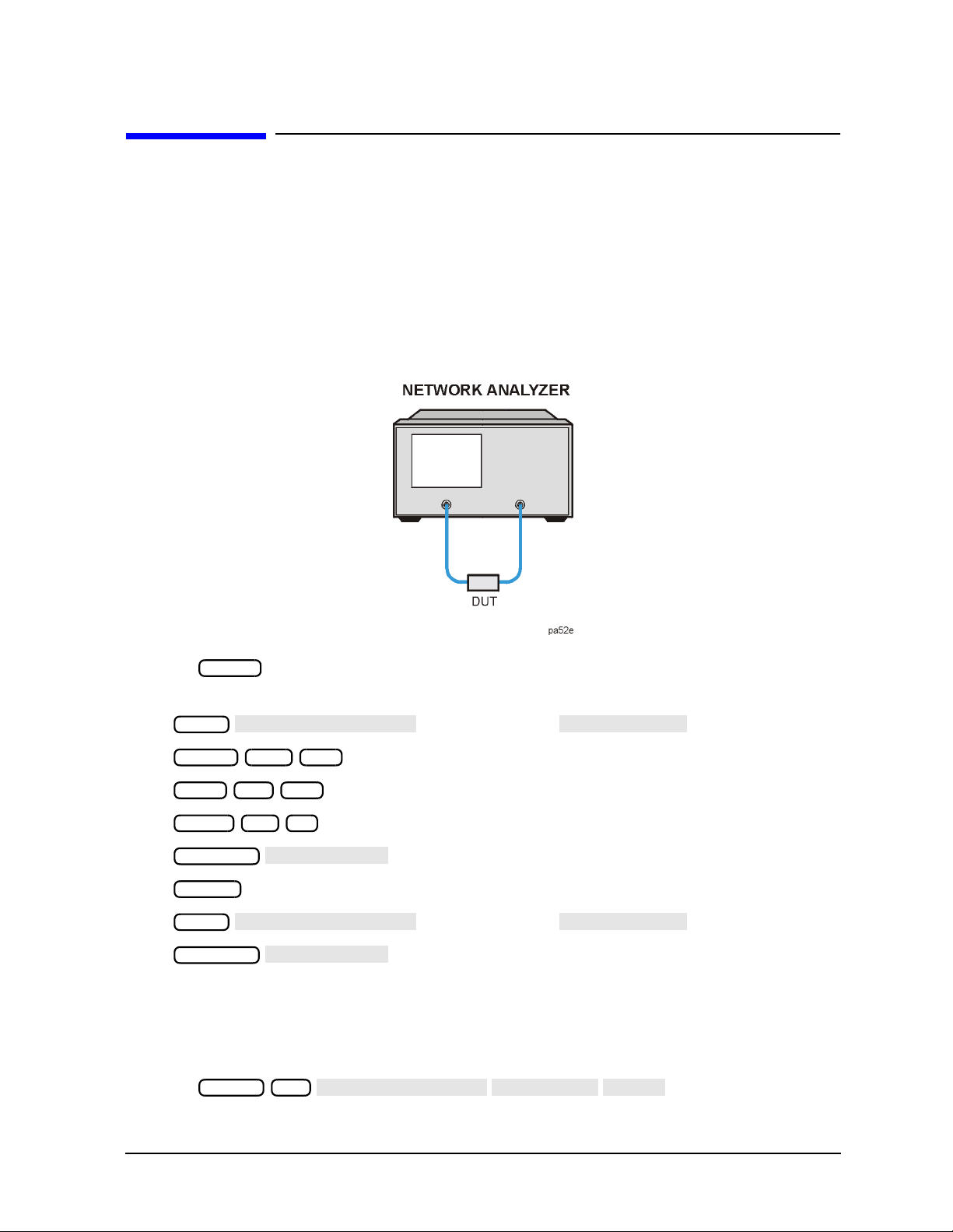
Step 1. Connect the device under test and any required test equipment.

1. Make the connections as shown in Figure 1-1.

Figure 1-1 Basic Measurement Setup

Step 2. Choose the measurement parameters.

Press . To set preset the analyzer to the “Factory Preset” conditions, press the

1-4

Preset

softkey if it is not selected. Then press .

Preset

Setting the Frequency Range

POWER RANGE MAN

POWER RANGES

NUMBER OF POINTS

Trans: FWD S21 (B/R)

TRANSMISSN

AUTOSCALE

SELECT DISK

INTERNAL MEMORY

RETURN

SAVE STATE

To set the center frequency to 134 MHz, press:

Center 134 M/µ

To set the span to 30 MHz, press:

Span 30 M/µ

Making Measurements

Making a Basic Measurement

NOTE You could also press the and keys and enter the frequency

Start Stop

range limits as start frequency and stop frequency values.

Setting the Source Power

To change the power level to −5 dBm, press:

Power −5 x1

NOTE You could also press and select

one of the power ranges to keep the power setting within the deﬁned range.

Setting the Measurement

To change the number of measurement data points to 101, press:

Sweep Setup

To select the transmission measurement, press:

Meas

or on ET models:

To view the data trace, press:

Scale Ref

Step 3. Perform and apply the appropriate error-correction.

Refer to the Chapter 5 , “Optimizing Measurement Results,” for procedures on correcting measurement errors.

To save the instrument state and error-correction in the analyzer internal memory, press:

Save/Recall

1-5

Making Measurements

SEARCH: MAX

PRINT MONOCHROME

PLOT

Making a Basic Measurement

Step 4. Measure the device under test.

Replace any standard used for error-correction with the device under test. To measure the insertion loss of the bandpass ﬁlter, press:

Marker Search

Step 5. Output the measurement results.

To create a printed copy of the measurement results, press:

Copy

(or )

Refer to Chapter 4 , “Printing, Plotting, and Saving Measurement Results,” for procedures on how to set up a printer and deﬁne a print, plot, or save results.

1-6

Making Measurements

Trans:FWD S21 (B/R)

TRANSMISSN

AUTO SCALE

Trans:FWD S21 (B/R)

TRANSMISSN

AUTO SCALE

CALIBRATE MENU

RESPONSE

THRU

Measuring Magnitude and Insertion Phase Response

This measurement example shows you how to measure the maximum amplitude of a surface acoustic wave (SAW) ﬁlter and then how to view the measurement data in the phase format, which provides information about the phase response.

Measuring the Magnitude Response

1. Connect your test device as shown in Figure 1-2.

Figure 1-2 Device Connections for Measuring a Magnitude Response

2. Press and choose the measurement settings. For this example, the

Preset

measurement parameters are set as follows:

Meas Center 134 M/µ Span 50 M/µ Power −3 x1 Scale Ref Chan 2 Meas Scale Ref

or on ET models:

You may also want to select settings for the number of data points, averaging, and IF bandwidth.

3. Remove the device and connect the power cables together (thru) and perform a response calibration using the following key presses.

Press .

Chan 1 Cal

1-7

Making Measurements

AUTO SCALE

SEARCH: MAX

DUAL | QUAD SETUP

DUAL CHAN ON

PHASE

Measuring Magnitude and Insertion Phase Response

If the channels are coupled (the default condition), this calibration is valid for both channels.

4. Reconnect your test device.

5. To better view the measurement trace, press:

Scale Ref

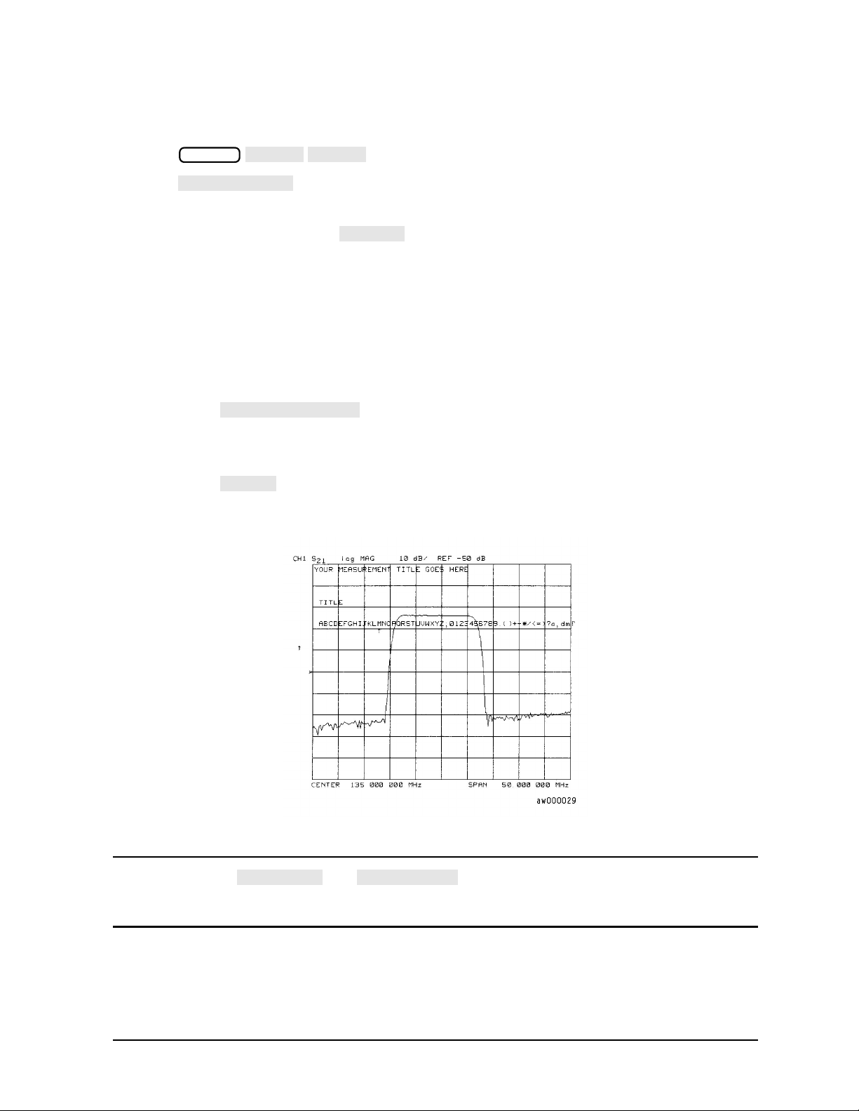
6. To locate the maximum amplitude of the device response, as shown in Figure 1-3, press:

Marker Search

Figure 1-3 Example Magnitude Response Measurement Results

Measuring Insertion Phase Response

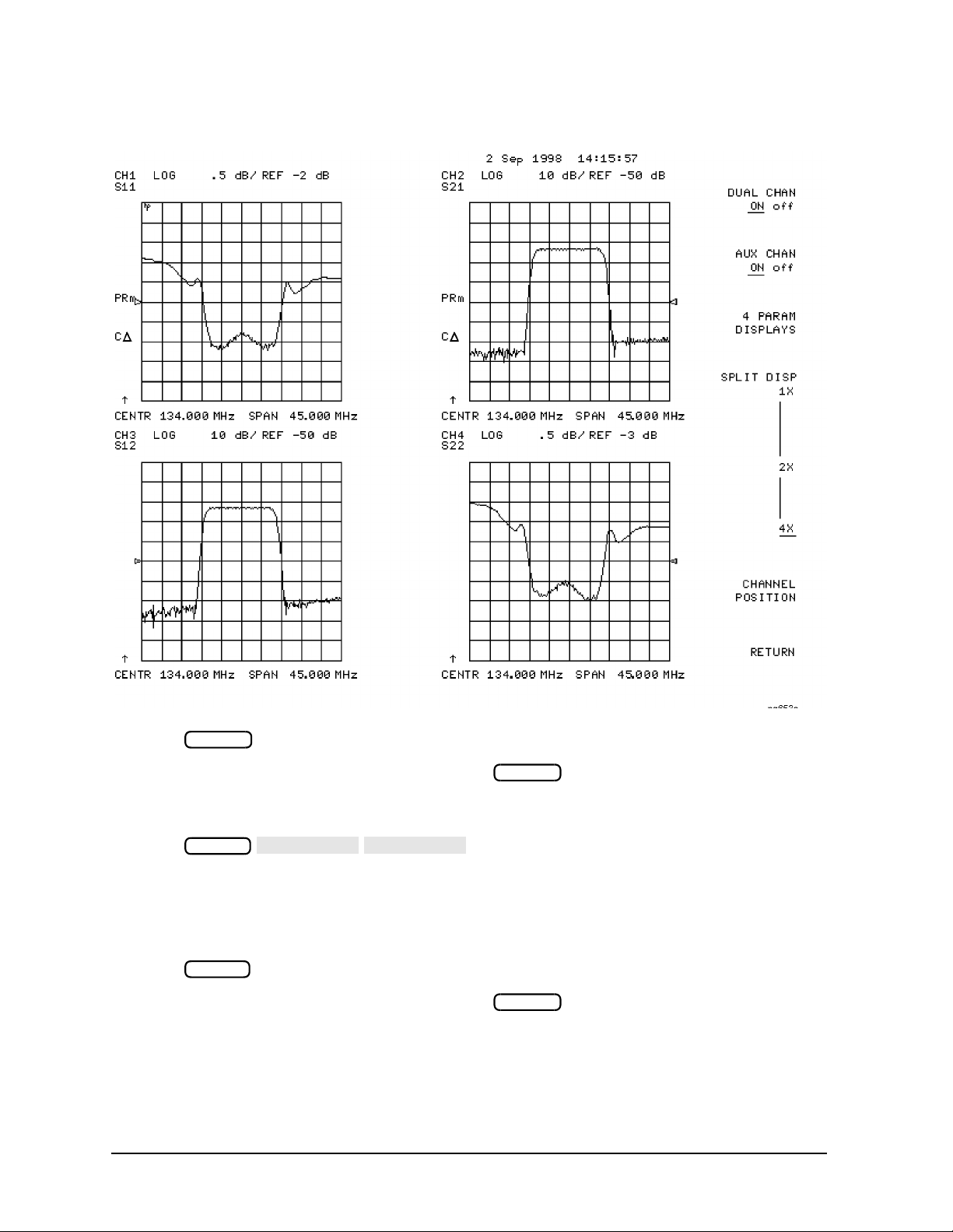
7. To view both the magnitude and phase response of the device, as shown in Figure 1-4, press:

Chan 2 Display Format

The channel 2 portion of Figure 1-4 shows the insertion phase response of the device under test. The analyzer measures and displays phase over the range of −180° to +180°. As phase changes beyond these values, a sharp 360° transition occurs in the displayed data.

1-8

Measuring Magnitude and Insertion Phase Response

Figure 1-4 Example Insertion Phase Response Measurement

Making Measurements

The phase response shown in Figure 1-5 is undersampled; that is, there is more than 180° phase delay between frequency points. If the ∆Φ ≥ 180°, incorrect phase and delay information may result. Figure 1-5 shows an example of phase samples being with ∆Φ less than 180° and greater than 180°.

Figure 1-5 Phase Samples

Undersampling may arise when measuring devices with long electrical length. To correct this problem, the frequency span should be reduced, or the number of points increased until ∆Φ is less than 180° per point. Electrical delay may also be used to compensate for this effect (as shown in the next example procedure).

1-9

Making Measurements

Using Display Functions

This section provides the necessary information for using the display functions. These functions are very helpful for displaying measurement data so that it will be easy to read. This section covers the following topics:

• Adding titles to your measurements

• Viewing both primary channels at the same time

• Viewing and customizing four-channel measurements

• Using the memory traces

• Using the memory math functions

• Blanking the analyzer’s display

• Changing the colors of the display

1-10

Titling the Active Channel Display

TITLE

ERASE TITLE

ENTER

SELECT LETTER

DONE

NEWLINE

FORMFEED

Making Measurements

Using Display Functions

1. Press to access the title menu.

Display

2. Press and enter the title you want for your measurement display.

• If you have a DIN keyboard attached to the analyzer, type the title you want from the keyboard. Then press to enter the title into the analyzer. You can enter

a title that has a maximum of 50 characters. (For more information on using a keyboard with the analyzer, refer to the “Options and Accessories” chapter in the reference guide.)

• If you do not have a DIN keyboard attached to the analyzer, enter the title from the analyzer front panel.

a. Turn the front panel knob to move the arrow pointer to the ﬁrst character of the

title.

b. Press . c. Repeat the previous two steps to enter the rest of the characters in your title. You

can enter a title that has a maximum of 50 characters.

d. Press to complete the title entry.

Figure 1-6 Example of a Display Title

CAUTION The and keys are not intended for creating display

titles. Those keys are for creating commands to send to peripherals during a sequence program.

1-11

Making Measurements

DUAL | QUAD SETUP

DUAL CHAN on OFF

SPLIT DISP

Using Display Functions

Viewing Both Primary Measurement Channels

In some cases, you may want to view more than one measured parameter at a time. Simultaneous gain and phase measurements, for example, are useful in evaluating stability in negative feedback ampliﬁers. You can easily make such measurements using the dual channel display.

1. To see channels 1 and 2 in the same grid, press:

Display

, set to ON, and

to 1X.

Figure 1-7 Example of Viewing Channel 1 and 2 Simultaneously

2. To view the measurements on separate graticules, press: Set to 2X. The analyzer shows channel 1 on the upper half of the display and channel 2 on the lower half of the display. The analyzer defaults to measuring S

on channel 1 and S21 on

channel 2.

1-12

Figure 1-8 Example Dual Channel with Split Display On

SPLIT DISPLAY 1X

COUPLED CH OFF

COUPLED CH ON off

MARKERS: UNCOUPLED

Making Measurements

Using Display Functions

3. To return to a single-graticule display, press: .

NOTE You can control the stimulus functions of the two channels independent of

each other by pressing .

Sweep Setup

Dual Channel Mode with Decoupled Stimulus

The stimulus functions of the two channels can be controlled independently using

in the stimulus menu. In addition, the markers can be controlled independently for each channel using in the marker mode menu, under the key.

Marker Fctn

NOTE ES models only: For dual channel, if channels are uncoupled and you have

full 2-port calibrations on both channels, you will not be able to select a non-ratioed measurement. For example, you can measure S

or B/R, but not

input B.

NOTE Auxiliary channels 3 and 4 are permanently coupled by stimulus to primary

channels 1 and 2, respectively. Decoupling the primary channels’ stimulus from each other does not affect the stimulus coupling between the auxiliary channels and their primary channels.

1-13

Making Measurements

MEASURE RESTART

AUX CHAN

DUAL | QUAD SETUP

DUAL CHAN

AUX CHAN

SPLIT DISP

Using Display Functions

Dual Channel Mode with Decoupled Channel Power

By decoupling the channel power or port power and using the dual channel mode, you can simultaneously view two measurements (or two sets of measurements, if both auxiliary channels are enabled) having different power levels.

However, there are situations where the analyzer will not update all measurements continuously. For analyzers with source attenuators, such situations occur if channel 1 requires one attenuation value and channel 2 requires a different value, or if 2-port cal is active and the port 1 attenuation value is not equal to the attenuation value of port 2. Since one attenuator is used for both measurements, this would cause the attenuator to continuously switch power ranges, which is not allowed.

If one of these conditions exist, the test set hold mode will engage, and the status notation tsH will appear on the left side of the screen. The hold mode leaves the measurement function in only one of the two measurement paths. To update both measurements, press

Sweep Setup

. Refer to "Source Attenuator Switch Protection" on

page 7-14.

Viewing Four Measurement Channels

Fourmeasurement channels can be viewed simultaneously by enabling auxiliary channels 3 and 4. Although independent of other channels in most variables, channels 3 and 4 are permanently coupled to channels 1 and 2 respectively by stimulus. That is, if channel 1 is set for a center frequency of 200 MHz and a span of 50 MHz, channel 3 will have the same stimulus values.

NOTE Channels 1 and 2 are referred to as primary channels and channels 3 and 4

are referred to as auxiliary channels.

Channel 3 or 4 are activated when the Chan 3 or Chan 4 keys are pressed. Alternatively, you can enable the auxiliary setting to ON. For example, if channel 1 is active, pressing to ON enables channel 3 and its trace appears on the display.

Channel 4 is similarly enabled and viewed when channel 2 is active.

1. Press to select the type of display of the data. This example uses the log mag

Format

format.

2. If channel 1 is not active, make it active by pressing .

3. Press , set to ON, set to

Display

Chan 1

ON, and set to . The display will appear as shown in Figure 1-9. Channel 1 is in the upper-left quadrant

of the display, channel 2 is in the upper-right quadrant, and channel 3 is in the lower half of the display.

1-14

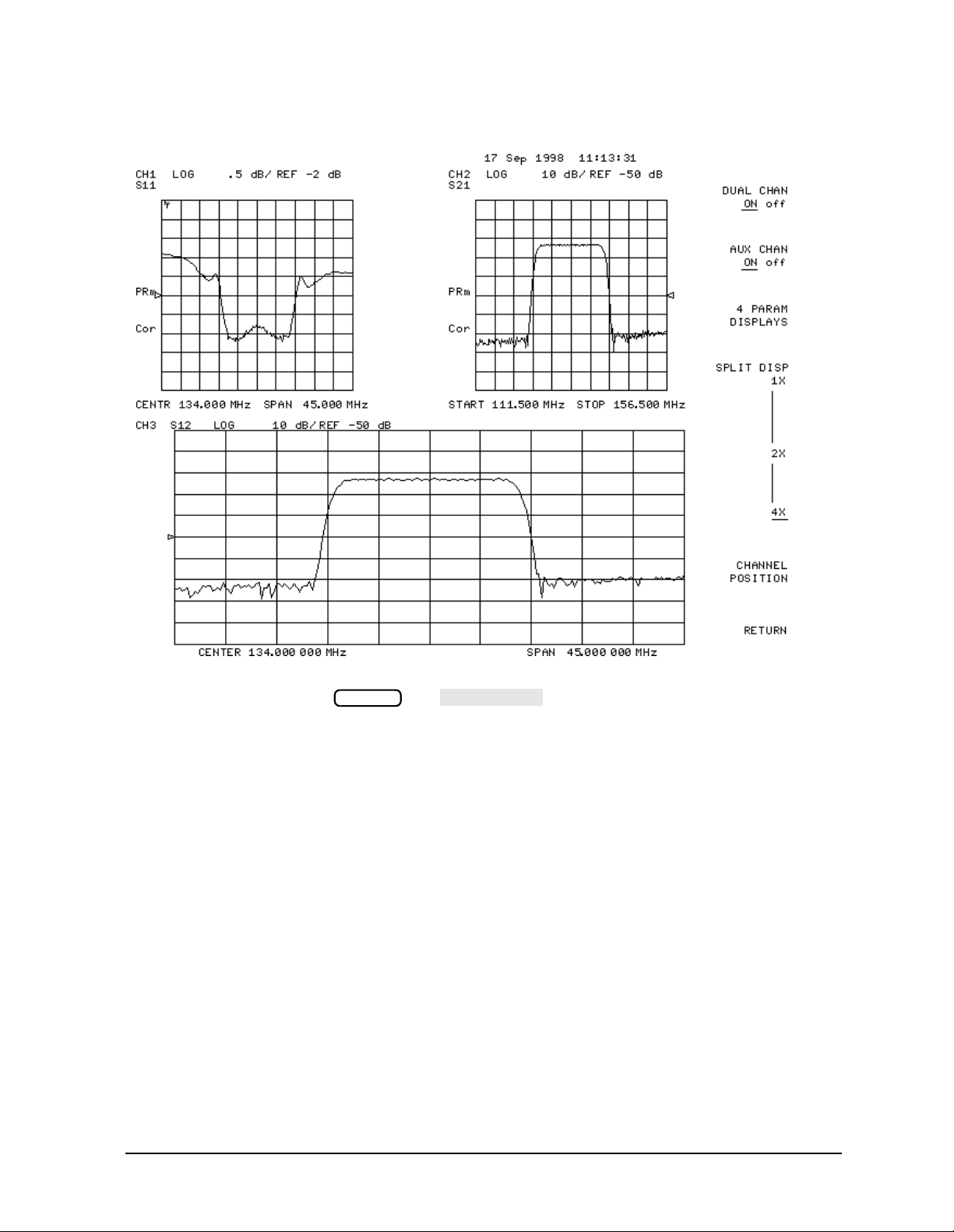
Figure 1-9 Three-Channel Display

AUX CHAN

Making Measurements

Using Display Functions

4. Press Chan 4 (or press , set to ON).

Chan 2

This enables channel 4 and the screen now displays four separate grids as shown in

Figure 1-10. Channel 4 is in the lower-right quadrant of the screen.

1-15

Making Measurements

MARKER 1

MARKER 2

Using Display Functions

Figure 1-10 Four-Channel Display

5. Press . Observe that the amber LED adjacent to the key is lit and the CH4 indicator

Chan 4

on the display has a box around it. This indicates that channel 4 is now active and can be conﬁgured.

6. Press .

Marker

Markers 1 and 2 appear on all four channel traces. Rotating the front panel control knob moves marker 2 on all four channel traces. Note that the active function, in this case the marker frequency, is the same color and in the same grid as the active channel (channel 4.)

7. Press . Observe that the amber LED adjacent to the key is lit. This indicates that

Chan 3

channel 3 is now active and can be conﬁgured.

8. Rotate the front panel control knob and notice that marker 2 still moves on all four channel traces.

1-16

9. To independently control the channel markers:

MARKER MODE MENU

MARKERS:

SMITH CHART

DUAL CHAN on OFF

SPLIT DISP 1X 2X 4X

CHANNEL POSITION

DUAL|QUAD SETUP

CHANNEL POSITION

SPLIT DISP 1X 2X 4X

SPLIT DISP 2X

CHANNEL POSITION

SPLIT DISP 4X

CHANNEL POSITION

Making Measurements

Using Display Functions

Press , set to UNCOUPLED.

Marker Fctn

Rotate the front panel control knob. Marker 2 moves only on the channel 3 trace.

Once made active, a channel can be conﬁgured independently of the other channels in most variables except stimulus. For example, once channel 3 is active, you can change its format

to a Smith chart by pressing .

Format

Customizing the Four-Channel Display

When one or both auxiliary channels are enabled, and

interact to produce different display conﬁgurations according to

Table 1-1

Table 1-1 Customizing the Display

Split Display Dual Channel Aux Channels On Number of Graticules

1X Don't Care Don't Care 1 1X/2X/4X Off None 2X/4X Off 3 or 4 2 2X On Don't Care 4X On 3 or 4 3 4X On Both on 4

Channel Position Softkey

gives you options for arranging the display of the channels. Press

Display

, to use .

works with . When is

selected, gives you two choices for a two-graticule display:

• Channels 1 and 2 overlaid in the top graticule, and channels 3 and 4 are overlaid in the bottom graticule.

• Channels 1 and 3 are overlaid in the top graticule, and channels 2 and 4 are overlaid in the bottom graticule.

When is selected, gives you two choices for a four-graticule display:

• Channels 1 and 2 are in separate graticules in the upper half of the display, channels 3 and 4 are in separate graticules in the lower half of the display.

• Channels 1 and 3 are in the upper half of the display, channels 2 and 4 are in the lower half of the display.

1-17

Making Measurements

4 PARAM DISPLAYS

SETUP A

SETUP F

SETUP A

SETUP B

TUTORIAL

MORE HELP

Using Display Functions

4 Param Displays Softkey

The menu does two things:

• provides a quick way to set up a four-parameter display

• gives information for using softkeys in the menu

Display

Figure 1-11 shows the ﬁrst screen. Six setup options are described

with softkeys through . is a four-parameter display where each channel is displayed on its own grid. Pressing immediately produces a four-grid, four-parameter display. is also a four-parameter display,

except that channel 1 and channel 2 are overlaid on the upper grid and channel 3 and channel 4 are overlaid on the lower grid. The other setup softkeys operate similarly. Notice that setups D and F produce displays which include Smith charts.

Pressing opens a screen which lists the order of keystrokes you would have to enter in order to create some of the setups without using one of the setup softkeys. The keystroke entries are listed (from top to bottom) beneath each setup and are color-coded to show the relationship between the keys and the channels. For example, beneath the four-grid display, [CHAN 1] and [MEAS] S11 are shown in yellow. Notice that in the four-grid graphic, Ch1 is also yellow, indicating that the keys in yellow apply to channel 1.

Pressing opens a screen which lists the hardkeys and softkeys associated with the auxiliary channels and setting up multiple-channel, multiple-grid displays. Next to each key is a description of its function.

Figure 1-11 4 Param Displays Menu

1-18

Making Measurements

DATA/MEM

DATA-MEM

DATA/MEM

DATA-MEM

DATA→MEMORY

Using Display Functions

Using Memory Traces and Memory Math Functions

The analyzer has four available memory traces, one per channel. Memory traces are totally channel dependent: channel 1 cannot access the channel 2 memory trace or vice versa. Memory traces can be saved with instrument states: one memory trace can be saved per channel for each saved instrument state. There are up to 31 save/recall registers available, so the total number of memory traces that can be present is 128 including the four active for the current instrument state. The memory data is stored as full precision, complex data. Memory traces must be displayed in order to be saved with instrument states.

Additional data can be stored onto 3.5-inch ﬂoppy disks using the front panel disk drive.

NOTE You may not be able to store 31 instrument states if they include a large

amount of calibration data. The calibration data contributes considerably to the size of the instrument state ﬁle and therefore the available memory may be full prior to ﬁlling all 31 registers.

Two trace math operations are implemented:

• (data/memory)

• (data−memory)

(Note that normalization is not .) Memory traces are saved and recalled and trace math is done immediately after error-correction. This means that any data processing done after error-correction, including parameter conversion, time domain transformation (Option 010), scaling, etc., can be performed on the memory trace. You can also use trace math as a simple means of error-correction, although that is not its main purpose.

All data processing operations that occur after trace math, except smoothing and gating, are identical for the data trace and the memory trace. If smoothing or gating is on when a memory trace is saved, this state is maintained regardless of the data trace smoothing or gating status. If a memory trace is saved with gating or smoothing on, these features can be turned on or off in the memory-only display mode.

The actual memory for storing a memory trace is allocated only as needed. The memory trace is cleared on instrument preset, power on, or instrument state recall.

If sweep mode or sweep range is different between the data and memory traces, trace math is allowed, and no warning message is displayed. If the number of points in the two traces is different, the memory trace is not displayed nor rescaled. However, if the number of points for the data trace is changed back to the number of points in the memory, the memory trace can then be displayed.

If trace math or display memory is requested and no memory trace exists, the message CAUTION: NO VALID MEMORY TRACE is displayed.

To Save a Data Trace to the Display Memory

Press to store the current active measurement data in the memory of the active channel. The data trace is now also the memory trace. You can use a memory trace for subsequent math manipulations.

Display

1-19

Making Measurements

MEMORY

DATA and MEMORY

DATA/MEM

DATA-MEM

COUPLED CH OFF

D2/D1 TO D2 ON

Using Display Functions

To View the Measurement Data and Memory Trace

The analyzer default setting shows you the current measurement data for the active channel.

1. To view a data trace that you have already stored to the active channel memory, press:

Display

This is the only memory display mode where you can change the smoothing and gating of the memory trace.

2. To view both the memory trace and the current measurement data trace, press:

Display

To Divide Measurement Data by the Memory Trace

You can use this feature for ratio comparison of two traces, for example, measurements of gain or attenuation.

1. You must have already stored a data trace to the active channel memory, as described in

"To Save a Data Trace to the Display Memory" on page 1-19.

2. Press to divide the data by the memory.

Display

The analyzer normalizes the data to the memory, and shows the results.

To Subtract the Memory Trace from the Measurement Data Trace

You can use this feature for storing a measured vector error, for example, directivity. Then, you can later subtract it from the device measurement.

1. You must have already stored a data trace to the active channel memory, as described in

"To Save a Data Trace to the Display Memory" on page 1-19.

2. Press to subtract the memory from the measurement data.

Display

The analyzer performs a vector subtraction on the complex data.

To Ratio Measurements in Channel 1 and 2

You may want to use this feature when making ampliﬁer measurements to produce a trace that represents gain compression. For example, with the channels uncoupled, you can increase the power for channel 2 while channel 1 remains unchanged. This will allow you to observe the gain compression on channel 2.

1. Press to uncouple the channels.

Sweep Setup

2. Make sure that both channels must have the same number of points.

3. Press to ratio channels 1 and 2, and put the results in the channel 2 data array. This ratio is applied to the complex data.

4. Refer to "Measuring Gain Compression" on page 1-60 for the procedure to identify the 1 dB compression point.

1-20

Display

Blanking the Display

ADJUST DISPLAY

BLANK DISPLAY

FREQUENCY BLANK

ADJUST DISPLAY

INTENSITY

DEFAULT COLORS

MODIFY COLORS

CH1 DATA/LIMIT LN

CH3 DATA/LIMIT LN

CH1 MEM

CH3 MEM

Making Measurements

Using Display Functions

Pressing switches off the analyzer

Display

display while leaving the instrument in its current measurement state. This feature may be helpful in prolonging the life of the LCD in applications where the analyzer is left unattended (such as in an automated test system). Turning the front panel knob or pressing any front panel key will restore normal display operation.

Pressing will blank the displayed frequency notation for

Display

security purposes. The frequency labels cannot be restored except by instrument preset or turning the power off and then on.

Adjusting the Colors of the Display

Setting Display Intensity

To adjust the intensity of the display, press and rotate the front panel knob, use the ( ) ( ) keys, or use the numerical keypad

to set the intensity value between 50 and 100 percent. Lowering the intensity may prolong the life of the LCD.

Setting Default Colors

To set all the display elements to the factory-deﬁned default colors, press

Display

NOTE does not reset or change colors to the default color values. However,

Preset

cycling power to the instrument will reset the colors to the default color values.

The Modify Colors Menu

The softkey within the adjust display menu provides access to the modify colors menu.

The modify colors menu allows you to adjust the colors on your analyzer's display. The default colors in this instrument were chosen to maximize your ability to discern the difference between the channel colors, and to comfortably and effectively view the colors. Each channel’s memory trace color was chosen because the color is similar to the channels data trace color.This allows easy association between the data trace and the memory trace for each channel.

You may choose to change the default colors to suit environmental needs, individual preferences, or to accommodate color deﬁcient vision. You can use any of the available colors for any of the display elements listed:

1-21

Making Measurements

CH2 DATA/LIMIT LN

CH4 DATA/LIMIT LN

CH2 MEM

CH4 MEM

GRATICULE

REF LINE

TEXT

WARNING

CH1 DATA

TINT

BRIGHTNESS

COLOR

Using Display Functions

To change the color of a display elements, press the softkey for that element (such as

). Then press and turn the analyzer front panel knob; use the step keys

or the numeric keypad, until the desired color appears.

NOTE Maximum viewing with the LCD display is achieved when primary colors or a

combination of them are selected at full brightness (100%). Table 1-2 lists the recommended colors and their corresponding tint numbers.

Table 1-2 Display Colors with Maximum Viewing Angle

Display Color Tint Brightness Color

Red 0 100 100 Yellow 17 100 100 Green 33 100 100 Cyan 50 100 100 Blue 67 100 100 Magenta 83 100 100 White N/A 100 0

Color is comprised of three parameters:

• Tint: The continuum of hues on the color wheel, ranging from red, through green and blue, and back to red.

• Brightness: A measure of the brightness of the color.

• Color: The degree of whiteness of the color. A scale from white to pure color.

The most frequently occurring color deﬁciency is the inability to distinguish red, yellow, and green from one another. Confusion between these colors can usually be eliminated by increasing the brightness between the colors. To accomplish this, press the

softkey and turn the analyzer front panel knob. If additional adjustment

is needed, vary the degree of whiteness of the color. To accomplish this, press the softkey and turn the analyzer front panel knob.

1-22

Making Measurements

SAVE COLORS

RECALL COLORS

Using Display Functions

NOTE Color changes and adjustments remain in effect until changed again in these

menus or the analyzer is powered off and then on again. Cycling the power changes all color adjustments to default values. Once the colors are saved,

pressing the key does not affect the color selections.

Preset

Saving Modiﬁed Colors

Tosave a modiﬁed color set, press .Modiﬁed colors are not part of a saved instrument state and are lost unless saved using these softkeys. Once modiﬁed colors are

saved, they will be the colors applied until is pushed.

Preset

Recalling Modiﬁed Colors

To recall the previously saved color set, press .

1-23

Making Measurements

MARKER MODE MENU

MARKERS: CONTINUOUS

MARKERS: DISCRETE

Using Markers

The key displays a movable active marker on the screen and provides access to a

Marker

series of menus to control up to ﬁve display markers for each channel. Markers are used to obtain numerical readings of measured values. They also provide capabilities for reducing measurement time by changing stimulus parameters, searching the trace for speciﬁc values, or statistically analyzing part or all of the trace.

Markers have a stimulus value (the x-axis value in a Cartesian format) and a response value (the y-axis value in a Cartesian format). In polar format, the second part of a complex data pair is also provided as an auxiliary response value. In Smith chart format, the real and imaginary rectangle are both displayed, and the effective capacitance or inductance of the imaginary part is also displayed. When a marker is activated and no other function is active, its stimulus value is displayed in the active entry area and can be controlled with the knob, the step keys, or the numeric keypad. The active marker can be moved to any point on the trace, and its response and stimulus values are displayed at the top right corner of the graticule for each displayed channel, in units appropriate to the display format. The displayed marker response values are valid even when the measured data is above or below the range displayed on the graticule.

• If you activate both data and memory traces, the marker values apply to the data trace.

• If you activate only the memory trace, the marker values apply to the memory trace.

• If you activate a memory math function (data/memory or data-memory), the marker values apply to the trace resulting from the memory math function.

Marker values are normally continuous: that is, they are interpolated between measured points. They can also be set to read only discrete measured points. Markers normally have the same stimulus values for all channels, or they can be uncoupled so that each channel has independent markers, regardless of whether stimulus values are coupled or dual channel display is on.

To Use Continuous and Discrete Markers

The analyzer can either place markers on discrete measured points, or move the markers continuously along a trace by interpolating the data value between measured points.

• Press and select one of the following choices: — Choose if you want the analyzer to place markers at

— Choose if you want the analyzer to place markers only on

Marker Fctn

any point on the trace, by interpolating between measured points. This default mode allows you to conveniently obtain round numbers for the stimulus value.

measured trace points determined by the stimulus settings. This may be the best mode to use with automated testing, using a computer or test sequencing because the analyzer does not interpolate between measured points.

1-24

Making Measurements

MARKERS: DISCRETE

MARKER 1

MARKER 2

MARKER 3

MARKER 4

MARKER 5

Using Markers

NOTE Using will also affect markersearchandpositioning

functions when the value entered in a search or positioning function does not exist as a measurement point. The marker will be positioned to the closest adjacent point that satisﬁes the search or positioning value.

To Activate Display Markers

• To switch on marker 1 and make it the active marker, press:

Marker

The active marker is identiﬁed on the analyzer display with the following symbol: ∇ The active marker stimulus value is displayed in the active entry area. You can modify

the stimulus value of the active marker, using the front panel knob or numerical keypad. All of the marker response and stimulus values are displayed in the upper right corner of the display.

Figure 1-12 Active Marker Control Example

To switch on the corresponding marker and make it the active marker, press:

All of the markers, other than the active marker, become inactive and are represented on the analyzer display as ∆. The active and inactive markers are shown in Figure 1-13.

, , or

1-25

Making Measurements

ALL OFF

1 2 3

MARKER MODE MENU

MARKERS:

Using Markers

Figure 1-13 Active and Inactive Markers Example

• To switch off all of the markers, press:

To Move Marker Information Off the Grids

If marker information obscures the display traces, you can turn off the softkey menu and move the marker information off the display traces and into the softkey menu area.

Pressing the backspace key performs this function. This is a toggle function. Pressing alternately hides and restores the current softkey menu. The softkey menu

is also restored when you press any softkey or a hardkey which leads to a menu.

1. Set up a four-graticule display as described in "Viewing Four Measurement Channels"

on page 1-14.

2. Activate four markers: Press .

NOTE Observe that the markers appear on all of the grids. To activate markers on

individual grids, press , and set

to UNCOUPLED. Then, activate the channel in which you wish

to have markers, press , then select the markers for that channel.

Marker

Marker Fctn

Marker

3. Turn off the softkey menu and move the marker information off the grids: Press . The display will be similar to Figure 1-14.

1-26

Making Measurements

Figure 1-14 Marker Information Moved into the Softkey Menu Area

Using Markers

pg654e

4. Restore the softkey menu and move the marker information back onto the graticules: Press .

The display will be similar to Figure 1-15.

1-27

Making Measurements

MODE MENU

REF=1

MARKER 2

Using Markers

Figure 1-15 Marker Information on the Graticules

pg655e

You can also restore the softkey menu by pressing a hardkey which opens a menu (such as

Meas

) or pressing a softkey.

To Use Delta (∆) Markers

This is a relative mode, where the marker values show the position of the active marker relative to the delta reference marker. You can switch on the delta mode by deﬁning one of the ﬁve markers as the delta reference.

1. Press to make marker 1 a reference marker.

Marker

∆

2. To move marker 1 to any point that you want to reference:

• Turn the front panel knob. OR

• Enter the frequency value (relative to the reference marker) on the numeric keypad.

3. Press and move marker 2 to any position that you want to measure in reference to marker 1.

∆

1-28

Figure 1-16 Marker 1 as the Reference Marker Example

MODE MENU

REF=2

MKR ZERO

MODE MENU

REF=∆FIXED MKR

MKR ZERO

FIXED MKR POSITION

MKR ZERO

MODE MENU

FIXED MKR POSITION

FIXED MKR STIMULUS

4. To change the reference marker to marker 2, press:

Making Measurements

Using Markers

∆

To Activate a Fixed Marker

When a reference marker is ﬁxed, it does not rely on a current trace to maintain its ﬁxed position. This is convenient when comparing two different measurement conditions. To

activate a ﬁxed marker on the analyzer, press . Marker zero puts a ﬁxed reference at the current position of the active marker.

To change to a Delta Marker to a ﬁxed reference marker, press

∆

Using the Key to Activate a Fixed Reference Marker

Marker zero enters the position of the active marker as the ∆ reference position. Alternatively, you can specify the ﬁxed point with . Marker zero

is canceled by switching delta mode off.

1. To place marker 1 at a point that you would like to reference, press:

Marker

and turn the front panel knob, or enter a value from the front panel keypad.

2. To measure values along the measurement data trace, relative to the reference point that you set in the previous step, press:

Marker

∆

keypad.

3. To move the reference position, press:

∆

front panel knob, or enter a value from the front panel keypad.

and turn the front panel knob, or enter a value from the front panel

and turn the

1-29

Making Measurements

REF=∆FIXED MKR

MODE MENU

REF=∆FIXED MKR

MODE MENU

FIXED MKR POSITION

FIXED MKR STIMULUS

FIXED MKR VALUE

FIXED MKR AUX VALUE

Using Markers

Figure 1-17 Example of a Fixed Reference Marker Using MKR ZERO

Using the Key to Activate a Fixed Reference Marker

∆

1. To set the frequency value of a ﬁxed marker that appears on the analyzer display, press:

Marker

∆

and turn the front panel knob, or

enter a value from the front panel keypad. The marker is shown on the display as a small delta (∆), smaller than∆ the inactive

marker triangles.

2. To set the response value (dB) of a ﬁxed marker, press: and turn the front panel knob, or enter a value from the front

panel keypad. In a Cartesian format, the setting is the y-axis value. In polar or Smith chart format,

with a magnitude/phase marker, a real/imaginary marker, an R+jX marker, or a G+jB marker, the setting applies to the ﬁrst part of the complex data pair. (Fixed marker response values are always uncoupled in the two channels.)

3. To set the auxiliary response value of a ﬁxed marker when you are viewing a polar or

Smith format, press:

and turn the front panel knob, or enter a value from the

front panel keypad. This value is the second part of complex data pair, and applies to a magnitude/phase

marker, a real/imaginary marker, an R+jX marker, or a G+jB marker. (Fixed marker auxiliary response values are always uncoupled in the two channels.)

1-30

Making Measurements

MARKER MODE MENU

MARKERS: COUPLED

MARKERS: UNCOUPLED

Using Markers

Figure 1-18 Example of a Fixed Reference Marker Using (∆)REF=(∆)FIXED MKR

To Couple and Uncouple Display Markers

At a preset state, the markers have the same stimulus values on each channel, but they can be uncoupled so that each channel has independent markers.

Press and select from the following keys:

Marker Fctn

• Choose if you want the analyzer to couple the marker stimulus values for the display channels.

• Choose if you want the analyzer to uncouple the marker stimulus values for the display channels. This allows you to control the marker stimulus values independently for each channel.

Figure 1-19 Example of Coupled and Uncoupled Markers

1-31

Making Measurements

LIN MKR

LOG MKR

Re/Im

MKR MODE MENU

MARKERS:DISCRETE

POLAR

MARKER MODE MENU

POLAR MKR MENU

LIN MKR

LOG MKR

Re/Im MKR

Using Markers

To Use Polar Format Markers

The analyzer can display the marker value as magnitude and phase, or as a real/imaginary pair: gives linear magnitude and phase, gives log magnitude and phase, gives the real value ﬁrst, then the imaginary value.

You can use these markers only when you are viewing a polar display format. (The format is available from the key.)

NOTE For greater accuracy when using markers in the polar format, it is

recommended to activate the discrete marker mode. Press

1. To access the polar markers, press:

Format

Marker Fctn

Format

Marker Fctn

2. Select the type of polar marker you want from the following choices:

• Choose if you want to view the magnitude and the phase of the active marker. The magnitude values appear in units and the phase values appear in degrees.

• Choose if you want to view the logarithmic magnitude and the phase of the active marker. The magnitude values appear in dB and the phase values appear in degrees.

• Choose if you want to view the real and imaginary pair, where the complex data is separated into its real part and imaginary part. The analyzer shows the real part as the ﬁrst marker value (M cos Θ), and the second value is the imaginary part (M sin Θ, where M = magnitude).

Figure 1-20 Example of a Log Marker in Polar Format

1-32

Making Measurements

MKR MODE MENU

MARKERS:DISCRETE

SMITH CHART

MARKER MODE MENU

SMITH MKR MENU

LIN MKR

LOG MKR

Re/Im MKR

R+jX MKR

G+jB MKR

Using Markers

To Use Smith Chart Markers

For greater accuracy when using markers in the Smith chart format, activate the discrete marker mode. Press .

To use Smith chart format:

Marker Fctn

1. Press .

2. Press and turn the front

Format Marker Fctn

panel knob, or enter a value from the front panel keypad to read the resistive and reactive components of the complex impedance at any point along the trace. This is the default Smith chart marker.

The marker annotation tells that the complex impedance is capacitive in the bottom half of the Smith chart display and is inductive in the top half of the display.

• Choose if you want the analyzer to show the linear magnitude and the phase of the reﬂection coefﬁcient at the marker.

• Choose if you want the analyzer to show the logarithmic magnitude and the phase of the reﬂection coefﬁcient at the active marker. This is useful as a fast method of obtaining a reading of the log magnitude value without changing to log magnitude format.

• Choose if you want the analyzer to show the values of the reﬂection coefﬁcient at the marker as a real and imaginary pair.

• Choose to show the real and imaginary parts of the device impedance (the series resistance and reactance, in ohms) at the marker. Also shown is the equivalent series inductance or capacitance.

• Choose to show the complex admittance values of the active marker in rectangular form. The active marker values are displayed in terms of conductance (in Siemens), susceptance, and equivalent parallel circuit capacitance or inductance. Siemens are the international unit of admittance and are equivalent to mhos (the inverse of ohms).

1-33

Making Measurements

MARKER→START

Using Markers

Figure 1-21 Example of Impedance Smith Chart Markers

To Set Measurement Parameters Using Markers

The analyzer allows you to set measurement parameters with the markers, without going through the usual key sequence. You can change certain stimulus and response parameters to make them equal to the current active marker value.

Setting the Start Frequency

1. Press and turn the front panel knob, or enter a value from the front panel

Marker Fctn

keypad to position the marker at the value that you want for the start frequency.

2. Press to change the start frequency value to the value of the active marker.

Figure 1-22 Example of Setting the Start Frequency Using a Marker

1-34

Setting the Stop Frequency

MARKER→STOP

MARKER→CENTER

Making Measurements

Using Markers

1. Press and turn the front panel knob, or enter a value from the front panel

Marker Fctn

keypad to position the marker at the value that you want for the stop frequency.

2. Press to change the stop frequency value to the value of the active marker.

Figure 1-23 Example of Setting the Stop Frequency Using a Marker

Setting the Center Frequency

1. Press and turn the front panel knob, or enter a value from the front panel

Marker Fctn

keypad to position the marker at the value that you want for the center frequency.

2. Press to change the center frequency value to the value of the active marker.

1-35

Making Measurements

MODE MENU

REF=1

MARKER 2

MARKER 1

MARKER 2

MKR ZERO

MARKER 1

MARKER→SPAN

Using Markers

Figure 1-24 Example of Setting the Center Frequency Using a Marker

Setting the Frequency Span

You can set the span equal to the spacing between two markers. If you set the center frequency before you set the frequency span, you will have a better view of the area of interest.

1. Press .

Marker

∆

2. Turn the front panel knob, or enter a value from the front panel keypad to position the markers where you want the frequency span.

Iterate between marker 1 and marker 2 by pressing and , respectively, and turning the front panel knob or entering values from the front panel keypad to position the markers around the center frequency. When ﬁnished positioning the markers, make sure that marker 2 is selected as the active marker.

NOTE Step 2 can also be performed using and . However,

when using this method, it will not be possible to iterate between marker zero and marker 1.

3. Press to change the frequency span to the range

Marker Fctn

between marker 1 and marker 2.

1-36

Figure 1-25 Example of Setting the Frequency Span Using Marker

MARKER→REFERENCE

Setting the Display Reference Value

Making Measurements

Using Markers

1. Press and turn the front panel knob, or enter a value from the front panel

Marker Fctn

keypad to position the marker at the value that you want for the analyzer display reference value.

2. Press to change the reference value to the value of the active marker.

Figure 1-26 Example of Setting the Reference Value Using a Marker

1-37

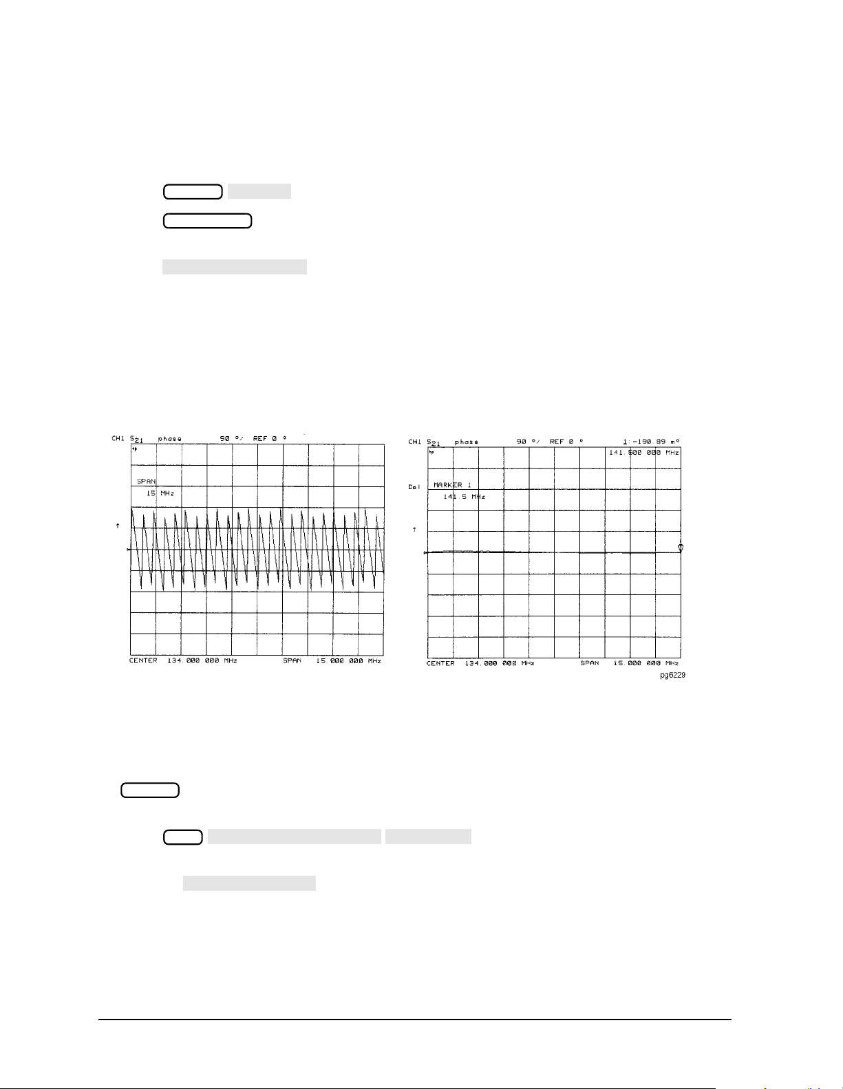
Making Measurements

PHASE

MARKER→DELAY

SPECIAL FUNCTIONS

MKR→CW

MKR→CW FREQ

Using Markers

Setting the Electrical Delay

This feature adds phase delay to a variation in phase versus frequency, therefore it is only applicable for ratioed inputs.

1. Press .

2. Press and turn the front panel knob, or enter a value from the front panel

Format Marker Fctn

keypad to position the marker at a point of interest.

3. Press to automatically add or subtract enough line length to the receiver input to compensate for the phase slope at the active marker position. This effectively ﬂattens the phase trace around the active marker. You can use this to measure the electrical length or deviation from linear phase.

Additional electrical delay adjustments are required on devices without constant group delay over the measured frequency span.

Figure 1-27 Example of Setting the Electrical Delay Using a Marker

Setting the CW Frequency

1. To place a marker at the desired CW frequency, press:

Marker

terminator.

2. Press . You can use this function to set the marker to a gain peak in an ampliﬁer. After

pressing , activate a CW frequency power sweep to look at the gain compression with increasing input power.

1-38

and either turn the front panel knob or enter the value, followed by a unit

Seq

Making Measurements

SEARCH: MAX

SEARCH: MIN

Using Markers

To Search for a Speciﬁc Amplitude

These functions place the marker at an amplitude-related point on the trace. If you switch on tracking, the analyzer searches every new trace for the target point.

Searching for the Maximum Amplitude

1. Press to access the marker search menu.

Marker Search

2. Press to move the active marker to the maximum point on the measurement trace.

Figure 1-28 Example of Searching for the Maximum Amplitude Using a Marker

Searching for the Minimum Amplitude

1. Press to access the marker search menu.

Marker Search

2. Press to move the active marker to the minimum point on the measurement trace.

1-39

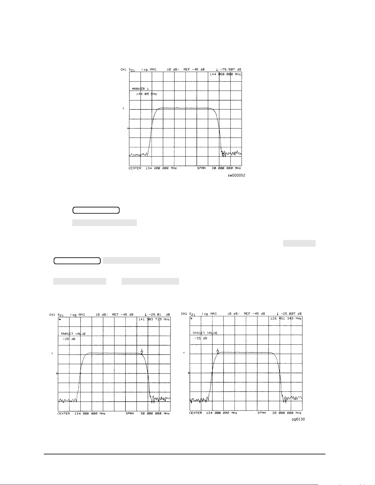
Making Measurements

SEARCH: TARGET

TARGET

TARGET VALUE

SEARCH LEFT

SEARCH RIGHT

Using Markers

Figure 1-29 Example of Searching for the Minimum Amplitude Using a Marker

Searching for a Target Amplitude

1. Press to access the marker search menu.

Marker Search

2. Press to move the active marker to the target point on the measurement trace.

3. If you want to change the target amplitude value (default is −3 dB), press and enter the new value from the front panel keypad. You may also press

Marker Search

to enter the new value.

4. If you want to search for multiple responses at the target amplitude value, press

and .

Figure 1-30 Example of Searching for a Target Amplitude Using a Marker

1-40

Making Measurements

SEARCH: MAX

MKR ZERO

WIDTHS ON

WIDTH VALUE

TRACKING ON

Using Markers

Searching for a Bandwidth

The analyzer can automatically calculate and display the bandwidth (BW:), center frequency (CENT:), Q, and loss of the device under test at the center frequency. (Q stands for “quality factor,” deﬁned as the ratio of a circuit's resonant frequency to its bandwidth.) These values are shown in the marker data readout.

1. Press and to place the marker near the center of the

Marker Search

ﬁlter passband.

2. Press if you want the bandwidth relative to the maximum.

3. Press to access the marker search menu.

Marker Search

4. Press to calculate the center stimulus value, bandwidth, and the Q of a bandpass or band reject shape on the measurement trace.

5. If you want to change the amplitude value (default is −3 dB) that deﬁnes the passband or reject band, press and enter the new value from the front panel

keypad.

Figure 1-31 Example of Searching for a Bandwidth Using Markers

Tracking the Amplitude that You Are Searching

1. Set up an amplitude search by following one of the previous procedures in "To Search

for a Speciﬁc Amplitude" on page 1-39.

2. Press to track the speciﬁed amplitude search with

Marker Search

every new trace and put the active marker on that point. When tracking is not activated, the analyzer ﬁnds the speciﬁed amplitude on the

current sweep and the marker remains at same stimulus value, regardless of changes in the trace response value with subsequent sweeps.

1-41

Making Measurements

MODE MENU

REF=1

MARKER 2

MKR MODE MENU

MKR STATS ON

Using Markers

To Calculate the Statistics of the Measurement Data

This function calculates the mean, standard deviation, and peak-to-peak values of the section of the displayed trace between the active marker and the delta reference. If there is no delta reference, the analyzer calculates the statistics for the entire trace.

1. Move marker 1 to any point that you want to reference:

• Turn the front panel knob. OR

• Enter the frequency value on the numeric keypad.

2. Press to make marker 1 a reference marker.

Marker

∆

3. Press and move marker 2 to any position that you want to measure in reference to marker 1.

4. Press to calculate and view the

Marker Fctn

mean, standard deviation, and peak-to-peak values of the section of the measurement data between the active marker and the delta reference marker.

An application for this feature is to ﬁnd the peak-to-peak value of passband ripple without searching separately for the maximum and minimum values.

If you are viewing a measurement in the polar or Smith Chart format, the analyzer calculates the statistics using the ﬁrst value of the complex pair (magnitude, real part, resistance, or conductance).

Figure 1-32 Example Statistics of Measurement Data

1-42

Making Measurements

Trans:FWD S21 (B/R)

TRANSMISSN

PHASE

AUTO SCALE

Measuring Electrical Length and Phase Distortion

Electrical Length

The analyzer mathematically implements a function similar to the mechanical “line stretchers” of earlier analyzers. This feature simulates a variable length lossless transmission line, which you can add to or remove from the analyzer's receiver input to compensate for interconnecting cables, etc. In this example, the electronic line stretcher measures the electrical length of a SAW ﬁlter.

Phase Distortion

The analyzer allows you to measure the linearity of the phase shift through a device over a range of frequencies and the analyzer can express it in two different ways:

• deviation from linear phase

• group delay

Measuring Electrical Length

1. Connect your test device as shown in Figure 1-33.

Figure 1-33 Device Connections for Measuring Electrical Length

2. Press and choose the measurement settings. For this example, the

Preset

measurement settings include reducing the frequency span to eliminate under-sampled phase response. Press the following keys as shown:

Meas

or on ET models:

Center 134 M/µ Span 2 M/µ Format Scale Ref

1-43

Making Measurements

CALIBRATE MENU

RESPONSE

THRU

AUTO SCALE

MARKER→DELAY

ELECTRICAL DELAY

Measuring Electrical Length and Phase Distortion

You may also want to select settings for the number of data points, averaging, and IF bandwidth.

3. Substitute a thru for the device and perform a response calibration by pressing:

Cal

4. Reconnect your test device.

5. To better view the measurement trace, press:

Scale Ref

Notice that in Figure 1-34 the SAW ﬁlter under test has considerable phase shift within only a 2 MHz span. Other ﬁlters may require a wider frequency span to see the effects of phase shift.

The linearly changing phase is due to the device's electrical length. You can measure this changing phase by adding electrical length (electrical delay) to compensate for it.

Figure 1-34 Linearly Changing Phase

6. To place a marker at the center of the band, press:

Marker

7. To activate the electrical delay function, press:

Marker Fctn

This function calculates and adds in the appropriate electrical delay by taking a ±10% span about the marker, measuring the ∆Φ, and computing the delay as the negative of ∆Φ / ∆ frequency.

Alternatively, press and turn the front panel knob to increase the electrical length until you achieve the best ﬂat line, as shown in Figure

1-44

and turn the front panel knob, or enter a value from the front panel keypad.

Scale Ref

Making Measurements

VELOCITY FACTOR

ELECTRICAL DELAY

Measuring Electrical Length and Phase Distortion

1-35.

The measurement value that the analyzer displays represents the electrical length of your device relative to the speed of light in free space. The physical length of your device is related to this value by the propagation velocity of its medium.

NOTE Velocity factor is the ratio of the velocity of wave propagation in a coaxial

cable to the velocity of wave propagation in free space. Most cables have a relative velocity of about 0.66 the speed in free space. This velocity depends on the relative permittivity of the cable dielectric (ε

Velocity Factor

) as

--------=

You could change the velocity factor to compensate for propagation velocity by pressing (enter the value) . This

Cal

will allow the analyzer to accurately display the equivalent distance that corresponds to the entered electrical delay.

Figure 1-35 Example Best Flat Line with Added Electrical Delay

8. To display the electrical length, press:

Scale Ref

In this example, there is a large amount of electrical delay due to the long electrical length of the SAW ﬁlter under test.

1-45

Making Measurements

SCALE DIV

MKR MODE MENU

STATS ON

Measuring Electrical Length and Phase Distortion

Measuring Phase Distortion

This portion of the example shows you how to measure the linearity of the phase shift over a range of frequencies. The analyzer allows you to measure this linearity and read it in two different ways: deviation from linear phase, or group delay.

Deviation From Linear Phase

By adding electrical length to “ﬂatten out” the phase response, you have removed the linear phase shift through your device. The deviation from linear phase shift through your device is all that remains.

1. Follow the procedure in "Measuring Electrical Length" on page 1-43.

2. To increase the scale resolution, press:

Scale Ref

and turn the front panel knob, or enter a value from the front

panel keypad.

3. To use the marker statistics to measure the maximum peak-to-peak deviation from linear phase, press:

Marker Fctn

4. Activate and adjust the electrical delay to obtain a minimum peak-to-peak value.

NOTE It is possible to use delta markers to measure peak-to-peak deviation in only

one portion of the trace. See "To Calculate the Statistics of the Measurement

Data" on page 1-42.

Figure 1-36 Deviation from Linear Phase Example Measurement

1-46

Making Measurements

DELAY

SCALE DIV

SMOOTHING ON

Measuring Electrical Length and Phase Distortion

Group Delay

The phase linearity of many devices is speciﬁed in terms of group or envelope delay. The analyzer can translate this information into a related parameter, group delay. Group delay is the transmission time through your device under test as a function of frequency. Mathematically, it is the derivative of the phase response which can be approximated by the following ratio:

−∆Φ /(360 ×∆Φ) where ∆Φ is the difference in phase at two frequencies separated by ∆F. The quantity ∆Fis

commonly called the “aperture” of the measurement. The analyzer calculates group delay from its phase response measurements.

The default aperture is the total frequency span divided by the number of points across the display (i.e. 201 points or 0.5% of the total span in this example).

1. Continue with the same instrument settings and measurements as in the previous procedure, “Deviation From Linear Phase.”

2. To view the measurement in delay format, as shown in Figure 1-37, press:

Format

Scale Ref

3. To activate a marker to measure the group delay at a particular frequency, press:

Marker

and turn the front panel knob, or enter a value from the front panel keypad.

Figure 1-37 Group Delay Example Measurement

Group delay measurements may require a speciﬁc aperture (∆)F) or frequency spacing between measurement points. The phase shift between two adjacent frequency points must be less than 180°, otherwise incorrect group delay information may result.

4. To vary the effective group delay aperture from minimum aperture (no smoothing) to approximately 1% of the frequency span, press: .

Avg

1-47

Making Measurements

SMOOTHING APERTURE

Measuring Electrical Length and Phase Distortion

When you increase the aperture, the analyzer removes ﬁne grain variations from the response. It is critical that you specify the group delay aperture when you compare group delay measurements.

Figure 1-38 Group Delay Example Measurement with Smoothing

5. To increase the effective group delay aperture, by increasing the number of measurement points over which the analyzer calculates the group delay, press:

As the aperture is increased the “smoothness” of the trace improves markedly, but at the expense of measurement detail.

Figure 1-39 Group Delay Example Measurement with Smoothing Aperture

Increased

1-48

Making Measurements

Measuring Electrical Length and Phase Distortion

Group delay is calculated by dividing the phase difference between points by the frequency spacing. Thus, if n equals the number of points, the number of phase difference values (or frequency segments) will be n−1. The ﬁrst data point is repeated so that the total number of points remains n.

1-49

Making Measurements

Characterizing a Duplexer (ES Analyzers Only)

This measurement example demonstrates how to characterize a 3-port device, in this case a duplexer, using four-parameter display mode. You must use a test adapter or a special 3-port test adapter to route the signals from the analyzer (a two-port instrument) to the duplexer (a three-port device). This example procedure is performed using one of the following test adapters:

❏ 8753D Option K36 Duplexer Test Adapter ❏ 8753D Option K39 3-Port Test Adapter ❏ 8753ES Option H39 3-Port Test Adapter (use the same instructions as those for K39

mode)

Deﬁnitions

The following abbreviations are used in reference to a duplexer:

Tx Transmitter port Ant Antenna port Rx Receiver port

Procedure

1. Press .

2. Connect the test adapter to the analyzer according to the instructions for your particular model. Connect any test ﬁxture or cables to the duplexer test adapter. Refer to Figure 1-40.

Preset

1-50

Figure 1-40 Duplexer Connections

COUPLED CH on OFF

OFF

CONFIGURE MENU

USER SETTINGS

K36 MODE on OFF

SELECT [TX-ANT]

K39 MODE on OFF

SELECT PORTS [1-3]

SAVE STATE

Making Measurements

Characterizing a Duplexer (ES Analyzers Only)

3. Set up channel 1 for the Tx-Ant stimulus parameters (start/stop frequency, power level, IF bandwidth). In this example, a wide frequency range that covers both the Tx-Ant and Ant-Rx parameters has been chosen.

4. Uncouple the primary channels from each other and then press and

Sweep Setup

toggle to .

5. Press .

System

6. Set up the desired mode.

• For K36 mode, toggle to ON. Then, press

Meas

• For K39 mode, toggle to ON. Then, press

Meas

7. Perform a full two-port calibration on channel 1 (refer to Chapter 6 , “Calibrating for

Increased Measurement Accuracy,” if necessary).

NOTE Make sure you connect the standards to the Tx port of the test adapter (or a

cable attached to it) for FORWARD calibrations, and to the Ant port for REVERSE calibrations.

8. Save the instrument state: Press .

9. Press .

10.Set up channel 2 for the Ant-Rx stimulus parameters. In this example, a wide frequency range that covers both the Tx-Ant and Ant-Rx parameters has been chosen.

Save/Recall Chan 2

1-51

Making Measurements

SELECT [RX-ANT]

SELECT PORTS [2-3]

SAVE STATE

DUAL|QUAD SETUP

4-PARAM DISPLAYS

SETUP B

Trans: REV S12 (A/R)

Reﬂ: REV S22 (B/R)

Trans:FWD S21 (B/R)

Reﬂ: FWD S11 (A/R)

DUAL CHAN on OFF

Characterizing a Duplexer (ES Analyzers Only)

11.Set up control of the test adapter so that channels 2 and 4 are Rx:

• For K36 mode, press .

• For K39 mode, press .

Meas Meas

12.Perform a full two-port calibration on channel 2.

NOTE Make sure you connect the standards to the Rx port of the test adapter (or a

cable attached to it) for FORWARD calibrations, and to the Ant port for REVERSE calibrations.

13.Save this state in the analyzer: Press .

Save/Recall

14.Connect the duplexer to the test adapter.

15.Set up a 2-graticule, 4-parameter display with transmission measurements on the top graticule and reﬂection measurements on the bottom graticule:

Press

Chan 4

Display

Chan 1

Meas

Chan 3

, then set to .

The display will be similar to Figure 1-41.

1-52

Figure 1-41 Duplexer Measurement

CONFIGURE MENU

TESTSET SW CONTINUOUS

CONFIGURE MENU

TESTSET SW CONTINUOUS

Making Measurements

Characterizing a Duplexer (ES Analyzers Only)

Normally, a 2-port calibration requires a forward and reverse sweep to complete before the displayed trace updates. Forfastertuning,it is possible to set the number of sweeps for the active display channel (S

and S21 for channel 1 in this case) to update more often than

the inactive display channel. In this example we choose 8 updates of the forward parameters to 1 update of the reverse in channel 1, and 8 updates of the reverse to 1 update of the forward in channel 2 (where the active parameters are S

Press . Press .

Chan 1 System Chan 2 System

and S12).

8 x1

1-53

Making Measurements

Measuring Ampliﬁers

The analyzer allows you to measure the transmission and reﬂection characteristics of many ampliﬁers and active devices. Youcan measure scalar parameters such as gain, gain ﬂatness,gain compression, reverse isolation, return loss (SWR), and gain drift versus time. Additionally, you can measure vector parameters such as deviation from linear phase, group delay, complex impedance and AM-to-PM conversion. You can also make high power measurements.

Figure 1-42 Ampliﬁer Parameters

When you are measuring a device that is very sensitive to absolute power level, it is important that you accurately set the power level at either the device input or output. The analyzer is capable of using an external GPIB power meter and controlling source power directly. Refer to Chapter 6 , "Calibrating for Increased Measurement Accuracy" for information on power meter calibration.

This section contains the following measurement examples:

• Measuring Harmonics (Option 002) on page 1-55

• Measuring Gain Compression on page 1-60

• Measuring Gain and Reverse Isolation Simultaneously (ES Analyzers Only) on page

1-64

• Making High Power Measurements with Option 014 (ES Analyzers Only) on page 1-66

1-54

Making Measurements

Measuring Ampliﬁers

Measuring Harmonics (Option 002)

The analyzer has the capability of measuring swept second and third harmonics as a function of frequency in a real-time manner. By using trace math, the second/third harmonic response can be displayed directly in dBc (dB below the fundamental or carrier). The ability to display harmonic level versus frequency or RF power allows “real-time” tuning of harmonic distortion.

Figure 1-43 Absolute Fundamental, 2nd, and 3rd Harmonic Output Levels

Figure 1-44 2nd and 3rd Harmonic Distortion in dBc

1-55

Making Measurements

INPUT PORTS

COUPLED CH OFF

CHAN POWER [COUPLED]

DUAL | QUAD SETUP

DUAL CHAN ON

HARMONIC MEAS

SECOND

Measuring Ampliﬁers

Making Harmonic Measurements

Perform the following steps to display the absolute power of the fundamental and second harmonic in dBm.

1. Press to measure the power for the fundamental

Chan 1 Meas

frequencies.

2. Press to measure the power for the harmonic

Chan 2 Meas

frequencies.

3. Set the start frequency to a value greater than 16 MHz.

4. Press and select . Uncoupling the channels allows

Sweep Setup

you to have the separate sweeps necessary for measuring the fundamental and harmonic frequencies.

5. Press and select . Coupling the channel power

Power

allows you to maintain the same fundamental frequency power level for both channels.

6. Press and set the power level for both channels.

7. Press and select .

8. Press and position marker to desired frequency.

9. Press . You can view both the fundamental

Power Display Marker System

power and harmonic power levels at the same time. (Refer to Figure 1-45.)

Figure 1-45 Fundamental and 2nd Harmonic Power Levels in dBm

1-56

Making Measurements

D2/D1 toD2 ON

Measuring Ampliﬁers

Toshow the second harmonic's power level relative to the fundamental power in dBc, press

Chan 2 Display

and select . This display mode lets you see the relationship between the fundamental and second or third harmonic in dBc. (Refer to

Figure 1-46.)

Figure 1-46 2nd Harmonic Power Level in dBc

Additional Harmonic Measurements

Vector network analyzers are commonly used to characterize ampliﬁer gain compression versus frequency and power level. This is essentially linear characterization since only the relative level of the fundamental input to the fundamental output is measured. The narrowband receiver is tuned to a precise frequency and, as a result, is immune from harmonic distortion. You may want to quantify the harmonic distortion itself. Figure 1-47 illustrates a simultaneous measurement of fundamental gain compression and second harmonic power as a function of input power.

1-57

Making Measurements

COUPLED PWR ON off

Measuring Ampliﬁers

Figure 1-47 Gain Compression and 2nd Harmonic Output Level

Understanding Harmonic Operation Single-Channel Operation You can view the second or third harmonic alone by using

only one of the analyzer's channels. Dual-Channel Operation To make the following types of measurements, uncouple

channels 1 and 2, and switch on dual channel.

• The analyzer measures the fundamental on one channel while measuring the second or third harmonic on the other channel.

• The analyzer measures the second harmonic on one channel while measuring the third harmonic on the other channel.

• Using the feature, the analyzer measures the fundamental on channel 1 while measuring the second or third harmonic in dBc on channel 2.

• Using the feature, the analyzer couples power between channels 1 and 2. This is useful when you are using the D2/D1 to D2 feature because you can change fundamental power and see the resultant change in the harmonic power.

The analyzer shows the fundamental frequency value on the display. However, a marker in the active entry area shows the harmonic frequency in addition to the fundamental. If you use the harmonic mode, the annotation H=2 or H=3 appears on the left-hand side of the display. The measured harmonic cannot not exceed the frequency limitations of the network analyzer's receiver.

1-58

Making Measurements

COUPLED PWR ON off

D2/D1 toD2 on OFF

COUPLED CHAN ON off

COUPLED PWR ON

Measuring Ampliﬁers

Coupling Power Between Channels 1 and 2 is intended to be used with the softkey. You can use the D2/D1 to D2 function in

harmonic measurements, where the analyzer shows the fundamental on channel 1 and the harmonic on channel 2. D2/D1 to D2 ratios the two, showing the fundamental and the relative power of the measured harmonic in dBc. You must uncouple channels 1 and 2 for

this measurement, using the softkey set to OFF to allow alternating sweeps.

After uncoupling channels 1 and 2, you may want to change the fundamental power and see the resultant change in relative harmonic power (in dBc). off

allows you to change the power of both channels simultaneously, even though they are uncoupled in all other respects.

Frequency Range The frequency range is determined by the upper frequency range of the instrument or system (3 or 6 GHz) and by the harmonic being displayed. The 6 GHz operation requires an 8753ET/ES Option 006. Table 1-3 shows the highest fundamental frequency for maximum frequency and harmonic mode.

Table 1-3 Maximum Fundamental Frequency using Harmonic Mode

Maximum Fundamental Frequency Harmonic Measured

2nd Harmonic 1.5 GHz 3.0 GHz 3rd Harmonic 1.0 GHz 2.0 GHz

8753ET/ES 8753ET/ES

Option 006

3 GHz 6 GHz

Accuracy and input power Refer to the “Speciﬁcations and Characteristics” chapter in the reference guide. The maximum recommended input power and maximum recommended source power are related speciﬁcations.

Using power levels greater than the recommended values may cause undesired harmonics in the source and receiver. The recommended power levels ensure that these harmonics are less than −45 dBc. Use test port power to limit the input power to your test device.

1-59

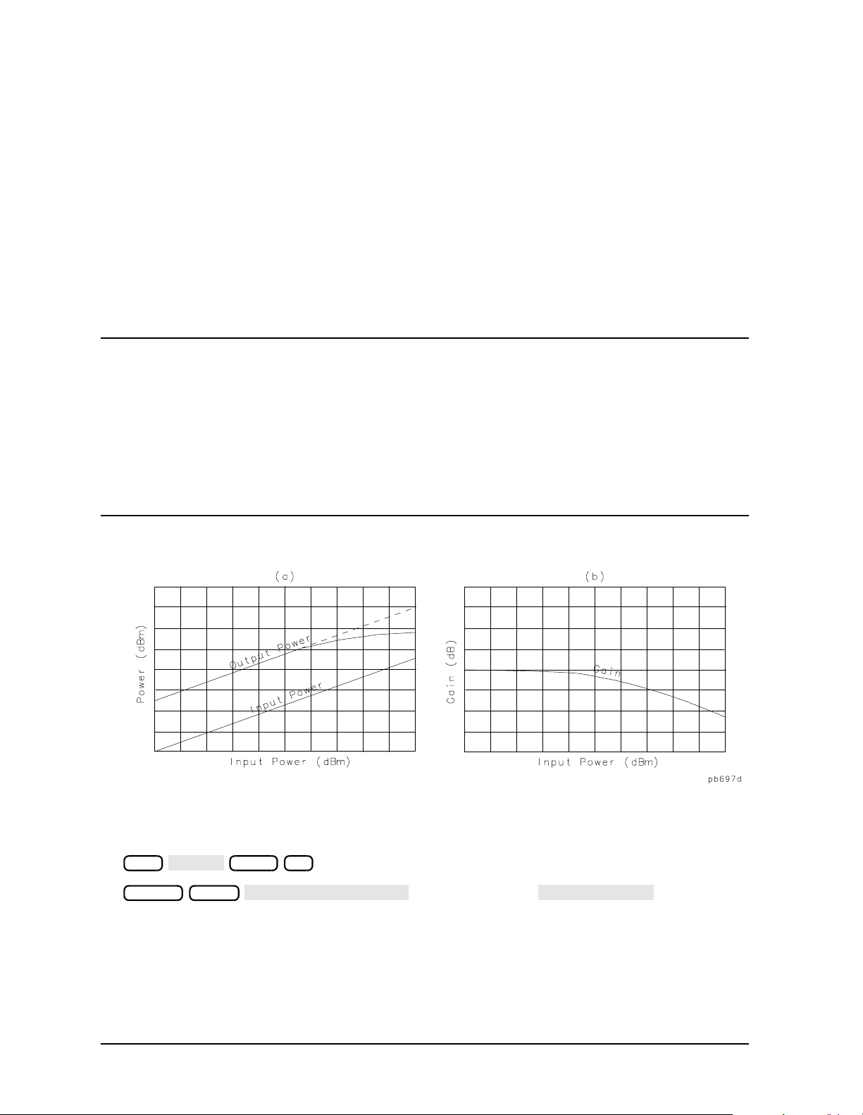
Making Measurements

IF BW

Trans:FWD S21 (B/R)

TRANSMISSN

Measuring Ampliﬁers

Measuring Gain Compression

Gain compression occurs when the input power of an ampliﬁer is increased to a level that reduces the gain of the ampliﬁer and causes a nonlinear increase in output power. The point at which the gain is reduced by 1 dB is called the 1 dB compression point. The gain compression will vary with frequency, so it is necessary to ﬁnd the worst-case point of gain compression in the frequency band.

Once that point is identiﬁed, you can perform a power sweep of that CW frequency to measure the input power at which the 1 dB compression occurs and the absolute power out (in dBm) at compression. The following steps provide detailed instruction on how to apply various features of the analyzer to accomplish these measurements.

NOTE In a compression measurement it is necessary to know the RF input or output

power at a certain level of gain compression. Therefore, both gain and absolute power level need to be accurately characterized. Uncertainty in a gain compression measurement is typically less than 0.05 dB. Also, each input channel of the analyzer is calibrated to display absolute power (typically within +0.5 dBm up to 3 GHz, and +1 dB up to 6 GHz). This can be improved by calibrating the power meter. Refer to "Power Meter

Measurement Calibration" on page 6-33 for information on calibrating the

power meter.

Figure 1-48 Diagram of Gain Compression

1. Set up the stimulus and response parameters for your ampliﬁer under test. To reduce the effect of noise on the trace, press:

Avg Chan 1 Meas

1000 x1

or on ET models:

2. Perform the desired error correction procedure. Refer to Chapter 6 , "Calibrating for

Increased Measurement Accuracy" for instructions on how to make a measurement

correction.

3. Connect the ampliﬁer under test.

1-60

Making Measurements

D1/D2 to D2 ON

DATA→MEMORY

DATA/MEM

DUAL | QUAD SETUP

DUAL CHANNEL ON

Trans:FWD S21 (B/R)

TRANSMISSN

COUPLED CH OFF

DISPLAY

D2/D1 to D2 ON

MARKER 1

SCALE/DIV

SEARCH:MIN

Measuring Ampliﬁers

4. To produce a normalized trace that represents gain compression, perform either step 5 or step 6. (Step 5 uses trace math and step 6 uses uncoupled channels and the display

function .)

5. Press to produce a normalized trace.

Display

6. To produce a normalized trace, perform the following steps:

• Press and select to view

Display

both channels simultaneously.

• Press or on ET models:

Chan 2 Meas

• To uncouple the channel stimulus so that the channel power will be uncoupled,

press:

Sweep Setup

This will allow you to separately increase the power for channel 2 and channel 1, so that you can observe the gain compression on channel 2 while channel 1 remains unchanged.

• To display the ratio of channel 2 data to channel 1 data on the channel 2 display,

press:

Chan 2

This produces a trace that represents gain compression only.

7. Press and position the marker at approximately mid-span.

8. Press to change the scale to 1 dB per division.

Marker Scale Ref

9. Press .

Power

10.Increase the power until you observe approximately 1 dB of compression on channel 2, using the step keys or the front panel knob.

11.To locate the worst case point on the trace, press:

Marker Search

1-61

Making Measurements

D2/D1 to D2 ON

COUPLED CH OFF

COUPLED CH ON

MARKER MODE MENU

MARKERS:DISCRETE

SPECIAL FUNCTIONS

MARKER→ CW

SWEEP TYPE MENU

POWER SWEEP

DUAL | QUAD SETUP

DUAL CHANNEL ON

D2/D1 to D2 ON

D2/D1 to D2 OFF

INPUT PORTS

SCALE/DIV

Measuring Ampliﬁers

Figure 1-49 Gain Compression Using Linear Sweep and

12.If was selected, recouple the channel stimulus by pressing:

Sweep Setup

13.To place the marker exactly on a measurement point, press:

Marker Fctn

14.To set the CW frequency before going into the power sweep mode, press:

Seq

15.Press .

Sweep Setup

If interpolation is on (the default setting), the calibration will be applied to the power sweep.

16.Enter the start and stop power levels for the sweep. Now channel 1 is displaying a gain compression curve. (Do not pay attention to channel

2 at this time.)

17.Press .

Chan 2 Display

18.If was selected, press .

19.Press .

Meas

Now channel 2 displays absolute output power (in dBm) as a function of power input.

20.Press to change the scale of channel 2 to 10 dB per division.

21.Press to change the scale of channel 1 to 1 dB per division.

1-62

Scale Ref

Chan 1 1 x1

10 x1

Making Measurements

MARKER MODE MENU

MARKERS:COUPLED

SEARCH:MAX

MKR ZERO

SEARCH:TARGET

MKR MODE MENU

MARKERS:UNCOUPLED

MODE MENU

MODE OFF

Measuring Ampliﬁers

NOTE A receiver calibration will improve the accuracy of this measurement. Refer

to Chapter 6 , “Calibrating for Increased Measurement Accuracy.”

22.Press .

Marker Fctn

23.To ﬁnd the 1 dB compression point on channel 1, press:

Marker Search

−1 x1

Marker

Marker Search

Notice that the marker on channel 2 tracked the marker on channel 1.

24.Press .

Chan 2 Marker

25.To take the channel 2 marker out of the ∆ mode so that it reads the absolute output power of the ampliﬁer (in dBm), press:

Marker

∆

Figure 1-50 Gain Compression Using Power Sweep

1-63

Making Measurements

COUPLED CH ON

PORT POWER [UNCOUPLED]

Trans:FWD S21 (B/R)

Trans: REV S12 (A/R)

DUAL | QUAD SETUP

DUAL CHAN ON

Measuring Ampliﬁers

Measuring Gain and Reverse Isolation Simultaneously (ES Analyzers Only)

Since an ampliﬁer will have high gain in the forward direction and high isolation in the reverse direction, the gain (S

Therefore, the power you apply to the input of the ampliﬁer for the forward measurement

) should be considerably lower than the power you apply to the output for the reverse

measurement (S

). By applying low power in the forward direction, you'll prevent the

ampliﬁer from being saturated. A higher power in the reverse direction keeps noise from being a factor in the measurement and accounts for any losses caused by attenuators or couplers on the ampliﬁer's output needed to lower the output power into the analyzer. The following steps demonstrate the features that best accomplish these measurements.

) will be much greater than the reverse isolation (S12).

1. Press .

Sweep Setup

Coupling the channels allows you to have the same frequency range and calibration applied to channel 1 and channel 2.

2. Press .

Power

Uncoupling the port power allows you to apply different power levels at each port. In

Figure 1-51, the port 1 power is set to −25 dBm for the gain measurement (S

port 2 power is set to 0 dBm for the reverse isolation measurement (S

3. Press and set the power level for port

Chan 1 Meas

Power

) and the

4. Press and set the power level for port

Chan 2 Meas

Power

5. Perform an error-correction and connect the ampliﬁer to the network analyzer. Refer to the Chapter 5 , “Optimizing Measurement Results,” for error-correction procedures.

6. Press .

Display

You can view both measurements simultaneously by using the dual channel display mode. Refer to Figure 1-51. If the port power levels are in different power ranges, one of the displayed measurements will not be continually updated and the annotation tsH will appear on the left side of the display. Refer to "Source Attenuator Switch

Protection" on page 7-14 for information on how to override this state.

NOTE To obtain best accuracy, you should set the power levels prior to performing

the calibration. However, the analyzer compensates for nominal power changes you make during a measurement, so that the error correction still remains quite valid. In these cases, the Cor annunciator will change to C∆.

1-64

Figure 1-51 Gain and Reverse Isolation

Making Measurements

Measuring Ampliﬁers

1-65

Making Measurements

Measuring Ampliﬁers

Making High Power Measurements with Option 014 (ES Analyzers Only)

Analyzers equipped with Option 014 can be conﬁgured to measure high power devices. This ability is useful if the required input power for a device under test is greater than the analyzer can provide or if the maximum output power from an ampliﬁer under test exceeds safe input limits for a standard analyzer. This section describes three conﬁgurations for performing high power measurements.

Figure 1-52 Internal Signal Paths of the Option 014 Analyzer

1-66

Making Measurements

Measuring Ampliﬁers

High Power Conﬁguration One

Figure 1-53 shows a one-path 2-port forward direction high power measurement. In this

conﬁguration the maximum power from test PORT 1 is 1 watt or 30 dBm. An external ampliﬁer and coupler are connected between the SWITCH and COUPLER access port for PORT 1. The coupled arm of the external coupler must be connected through an external switch to the R CHANNEL to maintain the phase lock in the forward direction.

NOTE This is only an example conﬁguration for high power applications. Actual

device values need to be determined for each individual application.

Figure 1-53 High Power Conﬁguration One

A power divider must be placed between the PORT 2 SWITCH and PORT 2 COUPLER ports with one leg of the divider connected through the external switch to the R CHANNEL port to maintain the phase lock in the reverse direction. (A coupler could also be used in place of the power divider.)

The recommended external switch for this application is the HP/Agilent 8762B Option T24. The maximum recommended power to the R CHANNEL input is −10 dBm, so depending on the coupling factor of the external coupler, an attenuator may need to be added to the R CHANNEL path.

Maximum power to PORT 2 is 2 watts or 33 dBm. Attenuators need to be added to the A and B sampler access ports to reduce the power to the A and B samplers. An additional attenuator must be added to the PORT 2 COUPLER/SWITCH ports to reduce the power to the transfer switch.

1-67

Making Measurements

Measuring Ampliﬁers

Control of the external switch can be done through the test set interface on the rear panel. Pin 8 on the TEST SET-I/O INTERCONNECT connector is a TTL 5 volt line that changes from TTL high in the forward measurement state to TTL low in the reverse measurement state. Refer to Figure 1-68 on page 1-95. Table 1-5 on page 1-97 is a complete listing of the connector’s pins.

Pin 1 on the external switch must be grounded. It can be grounded to:

• the analyzer's chassis

• the front panel binder post

• the outer shell of the TEST SET-I/O INTERCONNECT connector

• a ground pin on the TEST SET-I/O INTERCONNECT connector (pin 7, 12 or 18). Refer to Figure 1-68.

Pin C (common) on the HP/Agilent 8762B Option T24 must be connected to the test set interface Pin 14 (+22 volt line). Pin 2 on the 8762B Option T24 connects to Pin 8 (TTL 0) on the test set interface.

High Power Conﬁguration Two

Figure 1-54 shows a full 2-port forward direction high power measurement. In this

conﬁguration the maximum power from test PORT 1 and test PORT 2 is 0.10 watt or 20 dBm.

NOTE This is only an example conﬁguration for high power applications. Actual

device values need to be determined for each individual application.

Figure 1-54 High Power Conﬁguration Two

An external ampliﬁer and coupler are connected between the RF OUT and the RF IN access ports to the transfer switch.

The coupled arm of the external coupler must be connected to the R CHANNEL IN port. Maximum recommended power to the R CHANNEL input is −10 dBm, so depending on the coupling factor of the external coupler, an attenuator may need to be added to the R CHANNEL path.

1-68

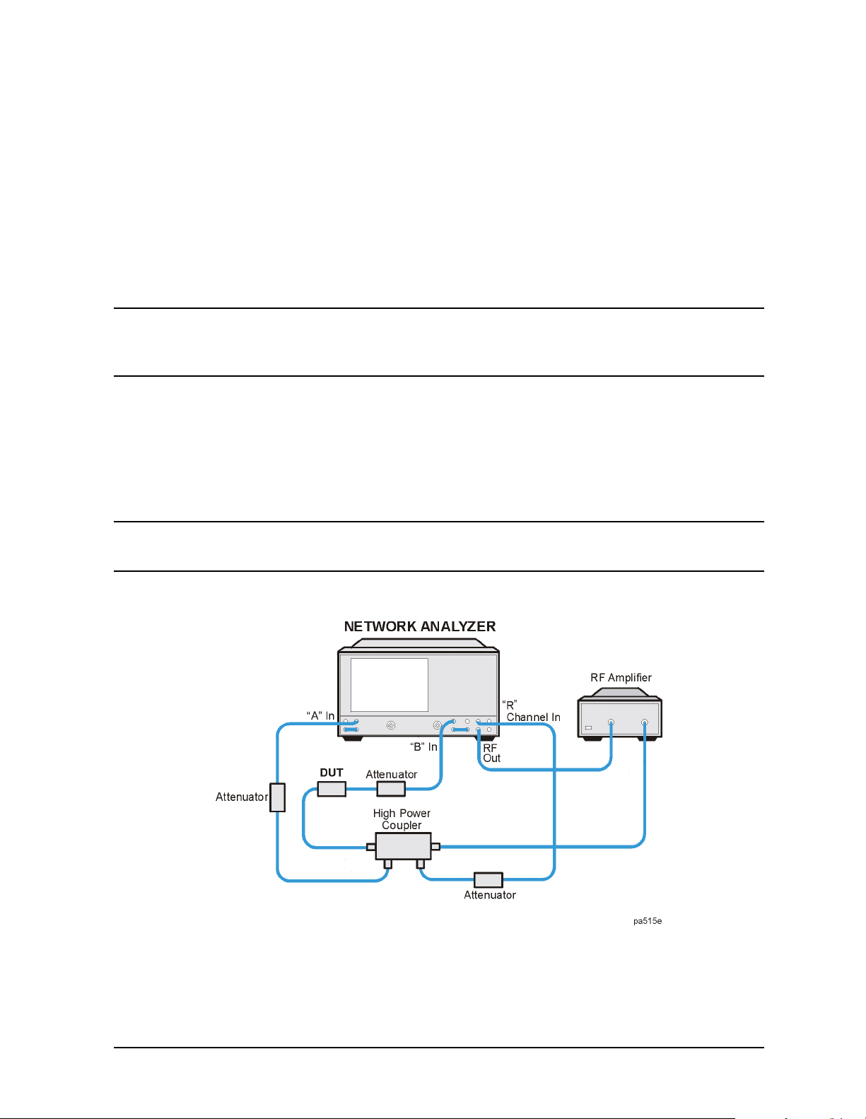
Making Measurements

Measuring Ampliﬁers

Maximum power to the RF IN port is 26 dBm. With the PORT 1 or PORT 2 SWITCH/COUPLER ports connected, the approximate loss from RF IN to either test PORT is 6 dB at 3 GHz, and 8 dB at 6 GHz. The approximate loss for the Option 075 is 8 dB at 3 GHz.

Maximum power to PORT 2 from the DUT is 2 watts or 33 dBm. Attenuators need to be added to the A and B sampler ports to reduce the power to the samplers. An isolator was added to the PORT 2 SWITCH/COUPLER ports to reduce power to the transfer switch. Maximum power to the transfer switch is 26 dBm. Some compression may occur above

−123 dBm.

NOTE Isolators must be inserted so that maximum isolation is achieved from the

COUPLER to the SWITCH ports. Refer to the isolators' manufacturer speciﬁcations for more information.

High Power Conﬁguration Three

Figure 1-55 shows the external high power conﬁguration. With this setup you can develop

your own high power conﬁguration. This solution can be used for measurements in the forward direction as long as the maximum power limits of the analyzer are not exceeded. This conﬁguration offers higher power capabilities.

NOTE This is only an example conﬁguration for high power applications. Actual

device values need to be determined for each individual application.

Figure 1-55 High Power Conﬁguration Three

1-69

Making Measurements

Using the Swept List Mode to Test a Device

When using a list frequency sweep, the analyzer has the ability to sweep arbitrary frequency segments, each containing a list of frequency points. One major advantage of using list frequency sweep is that it allows you to measure the minimum number of data points, and only at the frequencies of interest. This serves to minimize the overall test time. Two different list frequency sweep modes can be selected:

Stepped List Mode In this mode, the source steps to each deﬁned frequency point, stopping

while data is taken. This mode eliminates IF delay and allows frequency segments to overlap. However,the sweep time is substantially slower than for a continuous sweep with the same number of points.

Swept List Mode This mode takes data while sweeping through the deﬁned frequency

segments, increasing throughput by up to 6 times over a stepped sweep. In addition, this mode allows the test port power and IF bandwidth to be set independently for each segment that is deﬁned. The frequency segments in this mode cannot overlap.

The ability to completely customize the frequency sweep while using swept list mode is useful when setting up a measurement for a device with high dynamic range, like a ﬁlter. The following measurement of a ﬁlter illustrates the advantages of using the swept list mode.

• For in-depth information on swept list mode, refer to "Swept List Frequency Sweep

(Hz)" on page 7-18.

• For information on optimizing your measurement results when using swept list mode, refer to "To Use Swept List Mode" on page 5-9.

Connect the Device Under Test

1. Connect the equipment as shown in Figure 1-56.

Figure 1-56 Swept List Measurement Setup

1-70

2. Set the following measurement parameters:

Trans: FWD S21 (B/R)

TRANSMISSN

SWEEP TYPE MENU

EDIT LIST

Making Measurements

Using the Swept List Mode to Test a Device

Meas Center 900 M/µ Span 500 M/µ

or on ET models:

Observe the Characteristics of the Filter

Figure 1-57 Characteristics of a Filter

• Generally, the passband of a ﬁlter exhibits low loss. A relatively low incident power may be needed to avoid overdriving the next stage of the DUT (if that stage contains an ampliﬁer) or the network analyzer receiver.

• Conversely, the stopband of a ﬁlter generally exhibits high isolation. To measure this characteristic, the dynamic range of the system will have to be maximized. This can be done by increasing the incident power and narrowing the IF bandwidth.

Choose the Measurement Parameters

1. Decide the frequency ranges of the segments that will cover the stopbands and passband of the ﬁlter. For this example, the following ranges will be used:

• Lower stopband: 650 to 880 MHz

• Passband: 880 to 920 MHz

• Upper stopband: 920 to 1150 MHz

2. To set up the swept list measurement, press:

Sweep Setup

1-71

Making Measurements

ADD

START

STOP

NUMBER of POINTS

LIST POWER ON off

SEGMENT POWER

LIST IF BW ON off

SEGMENT IF BW

RETURN

DONE

ADD

CENTER

SPAN

STEP SIZE

SEGMENT POWER

SEGMENT IF BW

RETURN

DONE

ADD

START

STOP

NUMBER of POINTS

Using the Swept List Mode to Test a Device

Set Up the Lower Stopband Parameters

3. To set up the segment for the lower stopband, press

650 M/µ

880 M/µ

51 x1

4. To maximize the dynamic range in the stopband (increasing the incident power and narrowing the IF bandwidth), press

until ON is selected

10 x1

1000 x1

Set Up the Passband Parameters

5. To set up the segment for the passband, press

900 M/µ

40 M/µ

.2 M/µ

6. To specify a lower power level and a wider IF bandwidth for the passband, press

−10 x1

3700 x1

Set Up the Upper Stopband Parameters

7. To set up the segment for the upper stopband, press

8. To maximize the dynamic range in the stopband (increasing the incident power and narrowing the IF bandwidth), press:

1-72

920 M/µ

1150 M/µ

51 x1

Making Measurements

SEGMENT POWER

SEGMENT IF BW

RETURN

DONE

LIST FREQ [SWEPT]

Using the Swept List Mode to Test a Device

10 x1

300 x1

9. Press .

Calibrate and Measure

1. Remove the DUT and perform a full two-port calibration. Refer to Chapter 6 ,

“Calibrating for Increased Measurement Accuracy.”

2. With the thru connected, set the scale to autoscale to observe the beneﬁts of using swept list mode.

• The segments used to measure the stopbands have less noise, thus maximizing

dynamic range within the stopband frequencies.

• The segment used to measure the passband has been set up for faster sweep speed

with more measurement points.

Figure 1-58 Calibrated Swept List Thru Measurement

3. Reconnect the ﬁlter and adjust the scale to compare results with the ﬁrst ﬁlter measurement that used a linear sweep.

In Figure 1-59, notice that the noise level has decreased over 10 dB, conﬁrming that the noise reduction techniques in the stopbands were successful. Also, notice that the stopband noise in the third segment is slightly lower than in the ﬁrst segment. This is due to the narrower IF bandwidth of the third segment (300 Hz).

1-73

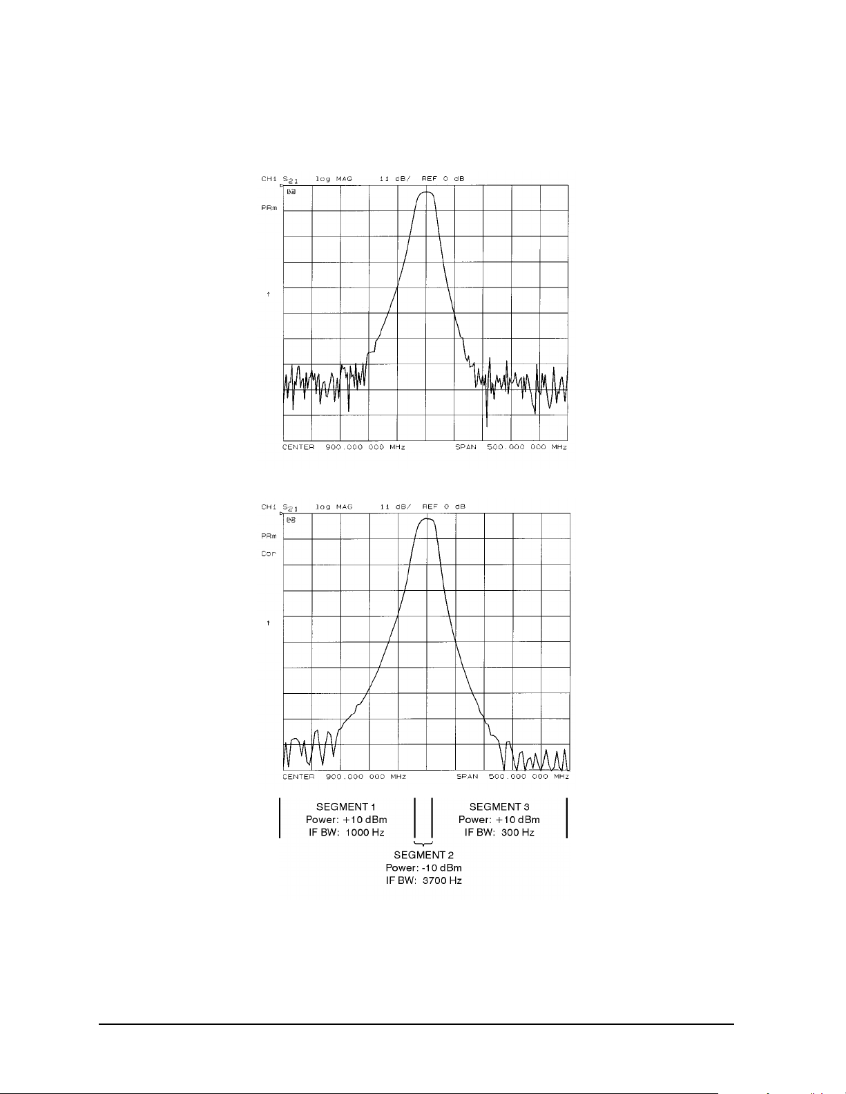
Making Measurements

Using the Swept List Mode to Test a Device

Figure 1-59 Filter Measurements Using Linear Sweep and Swept List Mode

Using Linear Sweep

(Power: 0 dBm/IF BW: 3700 Hz)

Using Swept List Mode

1-74

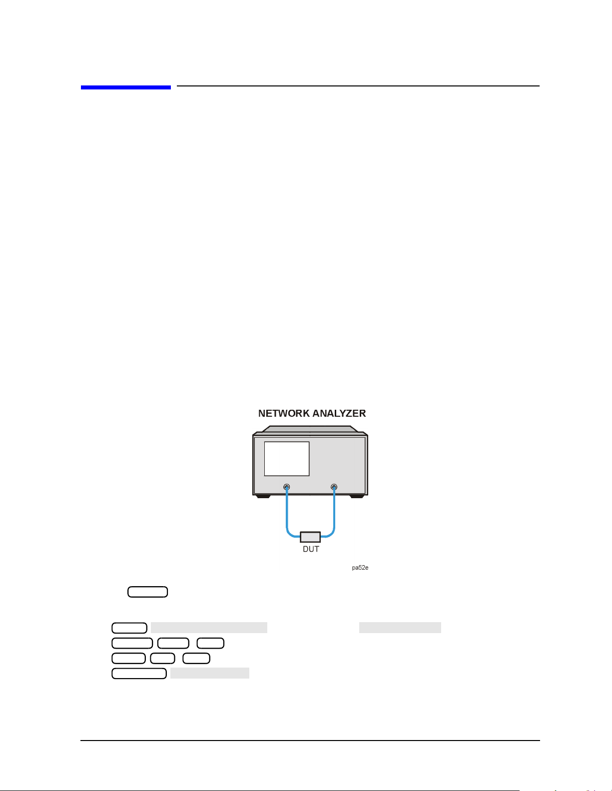
Making Measurements

Trans: FWD S21 (B/R)

TRANSMISSN

AUTO SCALE

Using Limit Lines to Test a Device

Limit testing is a measurement technique that compares measurement data to constraints that you deﬁne. Depending on the results of this comparison, the analyzer will indicate if your device either passes or fails the test.

Limit testing is implemented by creating individual ﬂat, sloping, and single-point limit lines on the analyzer display. When combined, these lines can represent the performance parameters for your device under test. The limit lines created on each measurement channel are independent of each other.

This example measurement shows you how to test a bandpass ﬁlter using the following procedures:

• creating ﬂat limit lines

• creating sloping limit lines

• creating single point limit lines

• editing limit segments

• running a limit test

Setting Up the Measurement Parameters

1. Connect your test device as shown in Figure 1-60.

Figure 1-60 Connections for SAW Filter Example Measurement

2. Press and choose the measurement settings. For this example the measurement settings are as follows:

• or on ET models:

•

Preset

Meas Center 134 M/µ Span 50 M/µ Scale Ref

You may also want to select settings for the number of data points, power, averaging, and IF bandwidth.

1-75

Making Measurements

CALIBRATE MENU

RESPONSE

THRU

AUTO SCALE

LIMIT MENU

LIMIT LINE ON

EDIT LIMIT LINE

CLEAR LIST

YES

ADD

STIMULUS VALUE

UPPER LIMIT

LOWER LIMIT

DONE

MIDDLE VALUE

DELTA LIMITS

MIDDLE VALUE

DELTA LIMITS

LIMIT TYPE

FLAT LINE

RETURN

Using Limit Lines to Test a Device

3. Substitute a thru for the device and perform a response calibration by pressing:

Cal

4. Reconnect your test device.

5. To better view the measurement trace, press:

Scale Ref

Creating Flat Limit Lines

In this example procedure, the following ﬂat limit line values are set:

Frequency Range Power Range

127 MHz to 140 MHz −27 dB to −21 dB 100 MHz to 123 MHz −200 dB to −65 dB 146 MHz to 160 MHz −200 dB to −65 dB

NOTE The minimum value for measured data is −200 dB.

1. To access the limits menu and activate the limit lines, press:

System

2. To create a new limit line, press:

The analyzer generates a new segment that appears on the center of the display.

3. To specify the limit's stimulus value, test limits (upper and lower), and the limit type, press:

127 M/µ

−21 x1

−27 x1

NOTE You could also set the upper and lower limits by using the

and keys. To use these keys for the entry, press:

−24 x1

3 x1

This would correspond to a test speciﬁcation of −24 ±3 dB.

4. To deﬁne the limit as a ﬂat line, press:

1-76

Making Measurements

ADD

STIMULUS VALUE

DONE

LIMIT TYPE

SINGLE POINT

RETURN

ADD

STIMULUS VALUE

UPPER LIMIT

LOWER LIMIT

DONE

LIMIT TYPE

FLAT LINE

RETURN

ADD

STIMULUS VALUE

DONE

LIMIT TYPE

SINGLE POINT

RETURN

Using Limit Lines to Test a Device

5. To terminate the ﬂat line segment by establishing a single point limit, press:

140 M/µ

Figure 1-61 shows the ﬂat limit lines that you have just created with the following

parameters:

• stimulus from 127 MHz to 140 MHz

• upper limit of −21 dB

• lower limit of −27 dB

Figure 1-61 Example Flat Limit Line

• To create a limit line that tests the low side of the ﬁlter, press:

100 M/µ

−65 x1

−200 x1

123 M/µ

1-77

Making Measurements

ADD

STIMULUS VALUE

UPPER LIMIT

LOWER LIMIT

DONE

LIMIT TYPE

FLAT LINE

RETURN

ADD

STIMULUS VALUE

DONE

LIMIT TYPE

SINGLE POINT

RETURN

Using Limit Lines to Test a Device

• To create a limit line that tests the high side of the bandpass ﬁlter, press:

146 M/µ

−65 x1

−200 x1

160 M/µ

Figure 1-62 Example Flat Limit Lines

Creating a Sloping Limit Line

This example procedure shows you how to make limits that test the shape factor of a SAW ﬁlter. The following limits are set:

Frequency Range Power Range

123 MHz to 125 MHz −65 dB to −26 dB 144 MHz to 146 MHz −26 dB to −65 dB

1-78

Making Measurements

LIMIT MENU

LIMIT LINE ON

EDIT LIMIT LINE

CLEAR LIST

YES

ADD

STIMULUS VALUE

UPPER LIMIT

LOWER LIMIT

DONE

LIMIT TYPE

SLOPING LINE

RETURN

ADD

STIMULUS VALUE

UPPER LIMIT

LOWER LIMIT

DONE

LIMIT TYPE

SINGLE POINT

RETURN

ADD

STIMULUS VALUE

UPPER LIMIT

LOWER LIMIT

DONE

LIMIT TYPE

SLOPING LINE

RETURN

ADD

STIMULUS VALUE

UPPER LIMIT

LOWER LIMIT

DONE

LIMIT TYPE

SINGLE POINT

RETURN

Using Limit Lines to Test a Device

1. To access the limits menu and activate the limit lines, press:

System

2. Toestablish the start frequency and limits for a sloping limit line that tests the low side of the ﬁlter, press:

123 M/µ

−65 x1

−200 x1

3. To terminate the lines and create a sloping limit line, press:

125 M/µ

−26 x1

−200

4. To establish the start frequency and limits for a sloping limit line that tests the high side of the ﬁlter, press:

144 M/µ

−26 x1

−200 x1

5. To terminate the lines and create a sloping limit line, press:

146 M/µ

−65 x1

−200 x1

You could use this type of limit to test the shape factor of a ﬁlter.

1-79

Making Measurements

LIMIT MENU

LIMIT LINE ON

EDIT LIMIT LINE

CLEAR LIST

YES

ADD

STIMULUS VALUE

UPPER LIMIT

LOWER LIMIT

DONE

LIMIT TYPE

SINGLE POINT

RETURN

ADD

STIMULUS VALUE

UPPER LIMIT

LOWER LIMIT

DONE

LIMIT TYPE

SINGLE POINT

RETURN

Using Limit Lines to Test a Device

Figure 1-63 Sloping Limit Lines

Creating Single Point Limits

In this example procedure, the following limits are set:

• from −23 dB to −28.5 dB at 141 MHz

• from −23 dB to −28.5 dB at 126.5 MHz

1. To access the limits menu and activate the limit lines, press:

System

2. To designate a single point limit line, as shown in Figure 1-64, you must deﬁne two pointers:

• downward pointing, indicating the upper test limit

• upward pointing, indicating the lower test limit Press:

−23 x1

−23

−28.5 x1

141

126.5 M/µ

M/µ

−28.5 x1

1-80

Figure 1-64 Example Single Points Limit Line

LIMIT MENU

LIMIT LINE ON

EDIT LIMIT LINE

SEGMENT

EDIT

UPPER LIMIT

DONE

LIMIT MENU

LIMIT LINE ON

EDIT LIMIT LINE

SEGMENT

DELETE

Editing Limit Segments

Making Measurements

Using Limit Lines to Test a Device

This example shows you how to edit the upper limit of a limit line.

1. To access the limits menu and activate the limit lines, press:

System

2. To move the pointer symbol (>) on the analyzer display to the segment you wish to modify, press:

or repeatedly OR and enter the segment number

followed by .

3. To change the upper limit (for example, −20) of a limit line, press:

−20 x1

Deleting Limit Segments

1. To access the limits menu and activate the limit lines, press:

System

2. To move the pointer symbol (>) on the analyzer display to the segment you wish to delete, press:

or repeatedly OR and enter the segment number

followed by .

3. To delete the segment that you have selected with the pointer symbol, press:

1-81

Making Measurements

LIMIT MENU

LIMIT LINE ON

EDIT LIMIT LINE

SEGMENT

LIMIT MENU

LIMIT TEST ON

BEEP FAIL ON

LIMIT LINE ON

BEEP FAIL ON

Using Limit Lines to Test a Device

Running a Limit Test

1. To access the limits menu and activate the limit lines, press:

System

Reviewing the Limit Line Segments

The limit table data that you have previously entered is shown on the analyzer display.

• To verify that each segment in your limits table is correct, review the entries by pressing:

and

• To modify an incorrect entry, refer to the procedure "Editing Limit Segments" on page

1-81.

Activating the Limit Test

To activate the limit test and the beep fail indicator, press:

System

NOTE Selecting the beep fail indicator is optional and will add

approximately 50 ms of sweep cycle time. Because the limit test will still work if the limits lines are off, selecting is also optional.

The limit test results appear on the right side on the analyzer display. The analyzer indicates whether the ﬁlter passes or fails the deﬁned limit test:

• The message FAIL will appear on the right side of the display if the limit test fails.

• The analyzer beeps if the limit test fails and if has been selected.

• The analyzer changes the color of the trace to ﬂashing red where the measurement

trace is out of limits.

• A TTL signal on the rear panel BNC connector "LIMIT TEST" provides a pass/fail

(5 V/0 V) indication of the limit test results.

Offsetting Limit Lines

The limit offset functions allow you to adjust the limit lines to the frequency and output level of your device. For example, you could apply the stimulus offset feature for testing tunable ﬁlters. Or, you could apply the amplitude offset feature for testing variable attenuators, or passband ripple in ﬁlters with variable loss.

This example shows you the offset feature and the limit test failure indications that can appear on the analyzer display.

1-82

Making Measurements

LIMIT MENU

LIMIT LINE OFFSETS

STIMULUS OFFSET

AMPLITUDE OFFSET

MARKER→ AMP. OFS.

AMPLITUDE OFFSET

Using Limit Lines to Test a Device

1. To offset all of the segments in the limit table by a ﬁxed frequency, (for example, 3 MHz), press:

System

3 M/µ

The analyzer beeps and a FAIL notation appears on the analyzer display, as shown in

Figure 1-65.

Figure 1-65 Example Stimulus Offset of Limit Lines

• To return to 0 Hz offset, press:

0 x1

• To offset all of the segments in the limit table by a ﬁxed amplitude, press:

5 x1

The analyzer beeps and a FAIL notation appears on the analyzer display.

• To return to 0 dB offset, press:

0 x1

• To offset the amplitude offset value by the active marker reading, press

. Pressing shows the current value.

1-83

Making Measurements

NEW SEQ/MODIFY SEQ

Using Test Sequencing

Testsequencing allows you to automate repetitive tasks. As you make a measurement, the analyzer memorizes the keystrokes. Later you can repeat the entire sequence by pressing a single key. Because the sequence is deﬁned with normal measurement keystrokes, you do not need additional programming expertise. Subroutines and limited decision-making increases the ﬂexibility of test sequences. In addition, the GPIO outputs can be controlled in a test sequence, and the GPIO inputs can be tested in a sequence for conditional branching.

The test sequence function allows you to create, title, save, and execute up to six independent sequences internally. You can also save sequences to disk and transfer them from the analyzer to another analyzer or possibly to an external computer controller (so the sequence can be sent to another analyzer).

How to Use Test Sequencing

The following procedures, which are based on an actual measurement example, show you how to do the following:

• create a sequence

• title a sequence

• edit a sequence

• clear a sequence

• change a sequence title

• name ﬁles generated by a sequence

• store a sequence

• load a sequence

• purge a sequence

• print a sequence

Creating a Sequence

1. To enter the sequence creation mode, press:

Seq

As shown in Figure 1-66, a list of instructions appear on the analyzer display to help you create or edit a sequence.

1-84

Figure 1-66 Test Sequencing Help Instructions

SEQUENCE 1 SEQ1

SELECT DISK

INTERNAL MEMORY

RETURN

RECALL STATE

Trans: FWD S21 (B/R)

TRANSMISSION

LOG MAG

AUTOSCALE

Making Measurements

Using Test Sequencing

2. To select a sequence position in which to store your sequence, press:

This choice selects sequence position #1. The default title is SEQ1 for this sequence. Refer to "Changing the Sequence Title" on page 1-89 for information on how to modify a

sequence title.

3. To create a test sequence, enter the parameters for the measurement that you wish to make. For this example, a SAW ﬁlter measurement is set up with the following parameters:

Save/Recall

Use the front panel knob to scroll until Preset State is highlighted on the display.

Meas Format Center 134 M/µ Span 50 M/µ Scale Ref

1-85

Making Measurements

DONE SEQ MODIFY

DO SEQUENCE

NEW SEQ/MODIFY SEQ

SEQUENCE 1 SEQ1

Using Test Sequencing

The previous keystrokes will create a displayed list as shown: Start of Sequence

RECALL PRST STATE Trans: FWD S21 (B/R) LOG MAG CENTER 134 M/u SPAN 50 M/u SCALE/DIV AUTO SCALE

4. To complete the sequence creation, press:

Seq

CAUTION When you create a sequence, the analyzer stores it in volatile memory where

it will be lost if you switch off the instrument power (except for sequence #6 which is stored in the analyzer non-volatile memory). However, you may store sequences to a ﬂoppy disk.

Running a Sequence

To run a stored test sequence, press:

Preset

and the softkey labeled with desired sequence number.

or, press:

Seq

and the softkey labeled with the desired sequence number

Stopping a Sequence

To stop a sequence before it has ﬁnished, press .

Local

Editing a Sequence

Deleting Commands

1. To enter the creation/editing mode, press:

Seq

2. To select the particular test sequence you wish to modify (sequence 1 in this example), press:

1-86

Making Measurements

DONE SEQ MODIFY

NEW SEQ/MODIFY SEQ

SEQUENCE 1 SEQ1

AVERAGING ON

DONE SEQ MODIFY

NEW SEQ/MODIFY SEQ

SEQUENCE 1 SEQ1

Using Test Sequencing

3. To move the cursor to the command that you wish to delete, press: or

• If you wish to scroll through the sequence without executing each line as you do so, you can press the key and scroll through the command list backwards.

• If you use the key to move the cursor through the list of commands, the commands are actually performed when the cursor points to them. This feature allows the sequence to be tested one command at a time.

4. To delete the selected command, press: (backspace key)

5. Press to exit the modify (edit) mode.

Seq

Inserting a Command

1. To enter the creation/editing mode, press:

Seq

2. To select the particular test sequence you wish to modify (sequence 1 in this example),

press:

3. To insert a command, move the cursor to the line immediately above the line where you

want to insert a new command, by pressing:

• If you wish to scroll through the sequence without executing each line as you do so, you can press the key and scroll through the command list backwards.

4. To enter the new command, press the corresponding analyzer front panel keys. For example, if you want to activate the averaging function, press:

Avg

5. Press to exit the modify (edit) mode.

Modifying a Command

1. To enter the creation/editing mode, press:

Preset Seq

2. To select the particular test sequence you wish to modify, (sequence 1 in this example), press:

Seq

1-87

Agilent 8753ES User's Guide

Specifications and Main Features

Frequently Asked Questions

User Manual

Documentation Map

1 Making Measurements

Using This Chapter

More Instrument Functions Not Described in This Guide

Making a Basic Measurement

Step 1. Connect the device under test and any required test equipment.

Step 2. Choose the measurement parameters.

Step 3. Perform and apply the appropriate error-correction.

Step 4. Measure the device under test.

Step 5. Output the measurement results.

Measuring Magnitude and Insertion Phase Response

Measuring the Magnitude Response

Measuring Insertion Phase Response

Using Display Functions

Titling the Active Channel Display

Viewing Both Primary Measurement Channels

Viewing Four Measurement Channels

Customizing the Four-Channel Display

Using Memory Traces and Memory Math Functions

Blanking the Display

Adjusting the Colors of the Display

Using Markers

To Use Continuous and Discrete Markers

To Activate Display Markers

To Move Marker Information Off the Grids

To Activate a Fixed Marker

To Couple and Uncouple Display Markers

To Use Polar Format Markers

To Use Smith Chart Markers

To Set Measurement Parameters Using Markers

Setting the CW Frequency

To Calculate the Statistics of the Measurement Data

Measuring Electrical Length and Phase Distortion

Measuring Electrical Length

Measuring Phase Distortion

Characterizing a Duplexer (ES Analyzers Only)

Procedure

Measuring Harmonics (Option 002)

Measuring Gain Compression

Measuring Gain and Reverse Isolation Simultaneously (ES Analyzers Only)

Making High Power Measurements with Option 014 (ES Analyzers Only)

Using the Swept List Mode to Test a Device

Connect the Device Under Test

Observe the Characteristics of the Filter

Choose the Measurement Parameters

Calibrate and Measure

Using Limit Lines to Test a Device

Setting Up the Measurement Parameters

Creating Flat Limit Lines

Creating a Sloping Limit Line

Creating Single Point Limits

Editing Limit Segments

Running a Limit Test

Offsetting Limit Lines

Using Test Sequencing

How to Use Test Sequencing

Creating a Sequence

Running a Sequence

Stopping a Sequence

Editing a Sequence