Agilent 8720D User’s Guide

Download

User’s Guide

Agilent Technologies

8719D/20D/22D

Network Analyzers

Manufacturing Part Number: 08720-90288

Printed in USA

Print Date: February 1999

Supersedes: October 1998

Hewlett-Packard to Agilent Technologies Transition

This manual may contain references to HP or Hewlett-Packard. Please note that Hewlett-Packard's former test and measurement, semiconductor products and chemical analysis businesses are now part of Agilent Technologies. To reduce potential confusion, the only change to product numbers and names has been in the company name prefix: where a product number/name was HP XXXX the current name/number is now Agilent XXXX. For example, model number HP478A is now model number Agilent 478A.

Documentation Warranty

THE MATERIAL CONTAINED IN THIS DOCUMENT IS PROVIDED "AS IS," AND IS SUBJECT TO BEING CHANGED, WITHOUT NOTICE, IN FUTURE EDITIONS. FURTHER, TO THE MAXIMUM EXTENT PERMITTED BY APPLICABLE LAW, AGILENT DISCLAIMS ALL WARRANTIES, EITHER EXPRESS OR IMPLIED WITH REGARD TO THIS MANUAL AND ANY INFORMATION CONTAINED HEREIN, INCLUDING BUT NOT LIMITED TO THE IMPLIED WARRANTIES OF MERCHANTABILITY AND FITNESS FOR A PARTICULAR PURPOSE. AGILENT SHALL NOT BE LIABLE FOR ERRORS OR FOR INCIDENTAL OR CONSEQUENTIAL DAMAGES IN CONNECTION WITH THE FURNISHING, USE, OR PERFORMANCE OF THIS DOCUMENT OR ANY INFORMATION CONTAINED HEREIN. SHOULD AGILENT AND THE USER HAVE A SEPARATE WRITTEN AGREEMENT WITH WARRANTY TERMS COVERING THE MATERIAL IN THIS DOCUMENT THAT CONFLICT WITH THESE TERMS, THE WARRANTY TERMS IN THE SEPARATE AGREEMENT WILL CONTROL.

DFARS/Restricted Rights Notice

If software is for use in the per formance of a U.S. Government prime contract or subcontract, Software is delivered and licensed as “Commercial computer software” as defined in DFAR 252.227-7014 (June 1995), or as a “commercial item” as defined in FAR

2.101(a) or as “Restricted computer sof tware” as defined in FAR 52.227-19 (June 1987) or any equivalent agency regulation or contract clause. Use, duplication or disclosure of Software is subject to Agilent Technologies’ standard commercial l icense terms, and non-DOD Departments and Agencies of the U.S. Government will receive no greater than Restricted Rights as defined in FAR 52.227-19(c)(1-2) (June 1987) . U.S. Government users will receive no greater than Limited Rights as defined in FAR 52.227-14 (June 1987) or DFAR 252.227-7015 (b)(2) (November 1995), as applicable in any technical data.

Printing Copies of Documentation from the Web

To print copies of documentation from the Web, download the PDF file from the Agilent web site:

•Go to http://www.agilent.com.

• Enter the document’s pa rt number (located on the title page) in the Quick Search box.

• Click GO.

• Click on the hyperlink for the document.

• Click the printer icon located in the tool bar.

Contacting Agilent

This information supersedes all prior HP contact information.

Online assistance: www.agilent.com/find/assist

Americas

Brazil

(tel) (+55) 11 3351 7012 (fax) (+55) 11 3351 7024

Canada

(tel) +1 877 894 4414 (fax) +1 303 662 3369

Mexico

(tel) 1 800 254 2440 (fax) 1 800 254 4222

Asia Pacific and Japan

Australia

(tel) 1 800 225 574 (fax) 1 800 681 776 (fax) 1 800 225 539

Japan (Bench)

(tel) 0120 32 0119 (alt) (+81) 426 56 7799 (fax) 0120 01 2144

Taiwan

(tel) 0800 047 669 (fax) 0800 047 667 (fax) 886 3492 0779

China

(tel) 800 810 0508 (alt) 800 810 0510 (fax) 800 810 0507 (fax) 800 810 0362

Japan (On-Site)

(tel) 0120 802 363 (alt) (+81) 426 56 7498 (fax) (+81) 426 60 895 3

Thailand

(tel) 1 800 2758 5822 (alt) (+66) 2267 5913 (fax) 1 800 656 336

Hong Kong (tel) 800 933 229 (fax) 800 900 701

Singapore

(tel) 1 800 275 0880 (fax) (+65) 675 5 1235 (fax) (+65) 675 5 1214

Malaysia

(tel) 1800 880 399 (fax) 1800 801 054

Europe

Austria

(tel) 0820 87 44 11* (fax) 0820 87 44 22

France

(tel) 0825 010 700* (alt) (+33) (0)1 6453 5623 (fax) 0825 010 701*

Italy

(tel) (+39) (0)2 9260 8484 (fax) (+39) (0)2 9544 1175

Spain

(tel) (+34) 91 631 3300 (alt) (+34) 91 631 3000 (fax) (+34) 91 631 3301

Switzerland (Italian)

(tel) 0800 80 5353 opt. 3* (alt) (+39) (0)2 9260 8484 (fax) (+41) (0)22 567 5314

(tel) = primary telephone number; (alt) = alternate telephone number; (fax) = FAX number; * = in country number

11/16/04

Belgium

(tel) (+32) (0)2 404 9340 (alt) (+32) (0)2 404 9000 (fax) (+32) (0)2 404 9395

Germany

(tel) 01805 24 6333* (alt) 01805 24 6330* (fax) 01805 24 6336*

Luxemburg

(tel) (+32) (0)2 404 9340 (alt) (+32) (0)2 404 9000 (fax) (+32) (0)2 404 9395

Sweden

(tel) 0200 88 22 55* (alt) (+46) (0)8 5064 8686 (fax) 020 120 2266*

United King dom

(tel) (+44) (0)7004 666666 (alt) (+44) (0)7004 123123 (fax) (+44) (0)7004 444555

Denmark

(tel) (+45) 7013 1515 (alt) (+45) 7013 7313 (fax) (+45) 701 3 1555

Ireland

(tel) (+353) (0)1 890 924 204 (alt) (+353) (0)1 890 924 206 (fax)(+353) (0)1 890 924 024

Netherlands

(tel) (+31) (0)20 547 2111 (alt) (+31) (0)20 547 2000 (fax) (+31) (0)20 547 2190

Switzerland (French)

(tel) 0800 80 5353 opt. 2* (alt) (+33) (0)1 6453 5623 (fax) (+41) (0)22 567 5313

United States

(tel) 800 829 4444 (alt) (+1) 303 662 3998 (fax) 800 829 4433

India

(tel) 1600 112 626 (fax) 1600 112 727 (fax) 1600 113 040

South Korea

(tel) 080 778 0011 (fax) 080 778 0013

Finland

(tel) (+358) 10 855 2100 (fax) (+358) (0) 10 855 2923

Israel

(tel) (+972) 3 9288 500 (fax) (+972) 3 9288 501

Russia

(tel) (+7) 095 797 3963 (alt) (+7) 095 797 3900 (fax) (+7) 095 797 3901

Switzerland (German )

(tel) 0800 80 5353 opt. 1* (alt) (+49) (0)7031 464 63 33 (fax) (+41) (0)1 272 7373

User’s Guide

HP 8719D/2OD/22D

Network Analyzer

HP Part No. 08720-90288 Supersedes: October 1998

Printed in USA February 1999

Notice.

The information contained in this document is subject to change without notice. Hewlett-Packard makes no warranty of any kind with regard to this material, including

but not limited to, the implied warranties of merchantability and fitness for a particular purpose. Hewlett-Packard shall not be liable for errors contained herein or for incidental or consequential damages in connection with the furnishing, performance, or use of this material.

Certification

Hewlett-Packard Company certifies that this product met its published specifications at the time of shipment from the factory. Hewlett-Packard further certifies that its calibration measurements are traceable to the United States National Institute of Standards and Technology, to the extent allowed by the Institute’s calibration facility, and to the calibration facilities of other International Standards Organization members.

Warranty

Note

The actual warranty on your instrument depends on the date it was ordered as well as whether or not any warranty options were purchased at that time.

determine the exact warranty on your instrument, contact the nearest Hewlett-Packard sales or service office with the model and serial number of your instrument. See the table titled “Hewlett-Packard

Sales

and Service

Offices,” later in this section, for a list of sales and service offices.

This Hewlett-Packard instrument product is warranted against defects in material and workmanship for the warranty period. During the warranty period, Hewlett-Packard Company will, at its option, either repair or replace products which prove to be defective.

If the warranty covers repair or service to be performed at Buyer’s facility, then the service or

repair will be performed at the Buyer’s facility at no charge within HP service travel areas. Outside HP service travel areas, warranty service will be performed at Buyer’s facility only upon HP’s prior agreement, and Buyer

shaIl

pay HP’s round-trip travel expenses. In all other

areas, products must be returned to a service facility designated by HP If the product is to be returned to Hewlett-Packard for service or repair, it must be returned

to a service facility designated by Hewlett-Packard. Buyer

shaIl

prepay shipping charges to Hewlett-Packard and Hewlett-Packard shall pay shipping charges to return the product to Buyer. However, Buyer

shaIl

pay

all

shipping charges, duties, and taxes for products returned

to Hewlett-Packard from another country. Hewlett-Packard warrants that its software and

use with an instrument will execute its progr

ilrmware designated by Hewlett-Packard for

amming

instructions when properly installed on that instrument. Hewlett-Packard does not warrant that the operation of the instrument, or software, or

Iirmware will

be uninterrupted or error-free.

LIMITATION OF WARRANTY

The foregoing warranty shall not apply to defects resulting from improper or inadequate maintenance by Buyer, Buyer-supplied software or interfacing, unauthorized modification or misuse, operation outside of the environmental specifications for the product, or improper site preparation or maintenance.

NO OTHER WARRANTY IS EXPRESSED OR IMPLIED. HEWLETT-PACKARD SPECIFICALLY DISCLAIMS THE IMPLIED

WmRANTIES

OF MERCHANTABILITY AND FITNESS FOR A

PARTICULAR PURPOSE.

XCLUSIVE REMEDIES

THE REMEDIES PROVIDED HEREIN ARE BUYER’S SOLE AND EXCLUSIVE REMEDIES. HEWLETT-PACKARD SHALL NOT BE LIABLE FOR ANY DIRECT, INDIRECT, SPECIAL, INCIDENTAL, OR CONSEQUENTIAL DAMAGES, WHETHER BASED ON CONTRACT, TORT, OR ANY OTHER LEGAL THEORY

. . .

III

Maintenance

Clean the cabinet using a damp cloth only.

Assistance

Product

Hewlett-Rzckurd products. I;br

maintenance

any

assistum

agreements

contact

gour

and other customer

nearest

Hewlett-&.&m-d

assisturn agrm

Sales and

semrice Om

are available for

Hewlett-Packard Sales and Service

FIELD OPERA!I’IONS

OfEces

Instrnment

Hewlett-Packard Company (800) 403-0801

IledqIlarters

Hewlett-Packard S.A. 160, Route du Nant-d’Avril 1217 Meyrin a/Geneva Switzerland (4122) 780.8111

Great Britain

Hewlett-Packard Ltd.

Eskdale Road, Winnersh Triangle

Wokingham, England

(44 734) 696622

HeadqMrters

Hewlett-Packard Company 3495 Deer Creek Road Palo Alto, 94304-1316 (416)

Support Center

Berkshire RG415DZ

California,

857-6027

USA

EUROPEAN FIELD OPERATIONS

Prance

Hewlett-Packard Prance Hewlett-Packard

1 Avenue Du Canada

Zone

D’Activite F-91947 Lea

France (49 6172) (33 1) 69 82 60 60

INTERCON FIELD OPERATIONS

AnstralIa

Hewlett-Packard Australia Ltd. Hewlett-Packard (Canada) Ltd.

31-41

Joseph Street Blackbum, Victoria 3130 (61 3) 895-2896

De Courtaboeuf

Ulis Cedex

h-Y

Hewlett-Packard 61352 Bad Homburg v.d.H

Germany

17500 South Service Road

TrausCanada Highway

Kirkland, Quebec

Canada

(614) 697-4232

GmbH Strasse

16-O

HQJ 2X&?

China Hewlett-Packard Company Hewlett-Packard Japan, Ltd.

38BeiSanHuanXlRoad

shuaug Yu shu

Hai Dian District Beijiq$

china

(86

253-6888

l]iiWLWl

Hewlett-Packard

8th Flooq

337 Fu

Ihipei, T&wan

(886

H-P Building

I-king

2) 712-0404

‘Ihiwan

North Road

9-l

%kakura-Cho, Hachioji

lbkyo

192, Japan

(81426) 60-2111

Japan

Singapore

Hewlett-Packard Singapore

150 Beach Road

#29-00

Gateway West Singapore 0718 (66) 291-9088

(Pte.)

Ltd.

Safety Symbols

The following safety symbols are used throughout this manual. of the symbols and its meaning before operating this instrument.

Caution

Warning

Caution denotes a hazard. It calls attention to a procedure that, if not correctly performed or adhered to, would result in damage to or destruction of the instrument. Do not proceed beyond a caution note until the indicated conditions are fully understood and met.

Wkning

correctly performed or adhered to, could result in injury or loss of life. Do not proceed beyond a warning note until the indicated conditions are fully understood and met.

denotes a hazard. It calls attention to a procedure which, if not

FamiIiarize

yourself with each

Instrument Markings

is necessary for the user to refer to the instructions in the documentation.

YE”

a year, it is when the design was proven.)

The instruction documentation symbol. The product is marked with this symbol when it

The CE mark is a registered trademark of the European Community. (If accompanied by

“ISMl-A”

“CSA” The CSA mark is a registered trademark of the Canadian Standards Association.

This is a symbol of an Industrial Scientific and Medical Group 1 Class A product.

General Safety Considerations

Warning

Caution

Warning

This is a ground incorporated in the power cord). The mains plug shall only be inserted in a socket outlet provided with a protective earth contact. Any interruption of the protective conductor, inside or outside the instrument, is likely to make the instrument dangerous. Intentional interruption is prohibited.

No operator serviceable parts inside. Refer servicing to personnel. To prevent electrical shock, do not remove covers.

Before switching on this instrument, make sure that the line voltage selector switch is set to the voltage of the power supply and the correct fuse is installed.

The opening of covers or removal of parts is likely to expose dangerous voltages. Disconnect the instrument from being opened.

The power cord is connected to internal capacitors that may remain live for 10 seconds after disconnecting the plug from its power supply.

safety

Class I product (provided with a protective earthing

qualilled

all voltage sources while it is

Warning

Note

For continued protection against fire hazard, replace line fuse only with same type and rating (F prohibited.

If this instrument is used in a manner not specilled by Co., the protection provided by the instrument may be impaired.

This instrument has been designed and tested in accordance with IEC Publication 348, Safety Requirements for Electronics Measuring Apparatus, and has been supplied in a safe condition. This instruction documentation contains information and warnings which must be operation and to maintain the instrument in a safe condition.

3A/250V).

The use of other fuses or material is

Hewlett-I%&a.rd

followed

by the user to ensure safe

vii

User’s Guide Overview

n Chapter 1, “HP

8719D/20D/22D

Description and Options,” describes features, functions, and

available options

n Chapter 2, “Making Measurements,” contains step-by-step procedures for making

measurements or using particular functions.

Chapter 3, “Making Mixer Measurements,”

contains step-by-step procedures for making

calibrated and error-corrected mixer measurements.

Chapter 4, “Printing, Plotting, and Saving Measurement Results, n contains instructions for saving to disk or the analyzer internal memory, and printing and plotting displayed measurements.

Chapter 5, “Optimizing Measurement Results,” describes techniques and functions for

achieving the best measurement results.

Chapter 6, “Application and Operation Concepts, n contains explanatory-style information

about many applications and analyzer operation.

n Chapter 7, “Specifications and Measurement Uncertainties,” defines the performance

capabilities of the analyzer.

n Chapter 8, “Menu n Chapter 9, “Key Definitions,” describes all the front panel keys, softkeys, and their

Maps,m

shows softkey menu relationships.

corresponding HP-IB commands.

n Chapter 10, “Error Messages,” provides information for interpreting error messages.

n Chapter 11, “Compatible Peripherals,

lists measurement and system accessories, and other applicable equipment compatible with the analyzer. Procedures for configuring the peripherals, and an HP-IB progr

Chapter 12, “Preset State and Memory Allocation, n contains a discussion of memory

amming

overview are also included.

allocation, memory storage, instrument state definitions, and preset conditions.

Appendix A, “The

the

CITItile

data format as well as a list of

CITIiile

Data Format and Key Word Reference, n contains information on

CITIille

keywords.

VIII

. .

Network Analyzer Documentation Set

The Installation and Quick Start Guide

familiarizes you with the network analyzer’s front and rear panels, electrical and environmental operating requirements, as well as procedures for installing, configuring, and verifying the operation of the analyzer.

The User’s Guide

measurements, explains commonly-used features, and tells you how to get the most performance from your analyzer.

The Quick Reference Guide

summary of selected user features.

The

Progmmm

programming information including an HP-IB programming and command reference as well as programming examples.

shows how to make

provides a

er’s

Guide

provides

The Service Guide

needed to adjust, troubleshoot, repair, and verify conformance to published specifications. Available with Option OBW.

provides the information

hanufacturer’s

DECLARATION OF CONFORMITY

Name:

accordq to ISWIEC Guide

Hewlett-Packard Co.

and

EN 45014

Manufacturer’s Address:

Microwave Instruments Division

1400 Fountaingrove Parkway Santa Rosa, CA USA

declares that the product

Product Name: Model Number: Product Options:

Network Analyzer

HP 87190, HP 87200, HP 87220

This declaration covers all options of the

above products.

conforms to the following Product specifications:

Safety: IEC

EMC:

lOlO-1:199O+Al

CANKSA-C22.2

/EN

No. 10

61010-1:1993

10.1-92

CISPR 11:199O/EN 55011:1991

IECEOl-2:1984/EN

50082-1:1992

Group 1, Class A

4 kVCD, 8

/EC EOl-3:1984/EN 50082-1:1992 3 V/m, 27-500 MHz /EC 801-4:1988IEN 50082-1:1992 0.5 kV Sig. Lines, 1 kV Power Lines

/EC 555-2: 1982 +A 1: 1985 / EN 60555-2: 1987

IEC

555-3:1982 +

A1:1990/

EN 60555-3:1987 +

95403-

kVAD

Al:1991

1799

Supplementary Information:

These products herewith comply with the requirements of the Low Voltage Directive

7U2ZYEEC

Santa Rosa, California, USA

Eumpean

and the EMC Directive 89/336/EEC

and

4 June 1996

Dixon Browder/Quality Manager

Contact: Your knxl Hewlett-Packard Sates and Service

HO-TRE, Hermnberger Stmse 130, D-71034 B6b@ten,

carry the CE-marking accordingly.

office or

Hewfett-Packard GmL#l,

Gennany

(FAX AS-7031-14-3143)

Department

Contents

EP 8719D/20D/22D

Where to Look for More Information Analyzer Description Front Panel Features Analyzer Display Rear Panel Features and Connectors Analyzer Options Available

Option

lD5,

Option 007, Mechanical Transfer Switch Option 085, High Power System Option 089, Frequency Offset Mode Option 012, Direct Access Receiver Configuration Option 400, Four-Sampler Option 010, Time Domain Option Option

lCM, lCP,

Rack Mount Flange Kit With Handles

Service and Support Options

BMcing

Measurements

Where to Look for More Information Principles of Microwave Connector Care Basic Measurement Sequence and Example

Basic Measurement Sequence Basic Measurement Example

Step 1. Connect the device under test and any required test equipment. Step 2. Choose the measurement parameters.

Setting the Frequency Range

Setting the Source

Setting the Measurement Step 3. Perform and apply the appropriate error-correction. Step 4. Measure the device under test. Step 5. Output the measurement results.

Using the Display Functions

To View Both Primary Measurement Channels To Save a Data Trace to the Display Memory

‘Ib

View the Measurement Data and Memory Trace To Divide Measurement Data by the Memory Trace To Subtract the Memory Trace from the Measurement Data Trace

‘IbRatioMeasurementsinChannel1and2 To Title

the Active Channel Display

Using the Four-Parameter Display

Four-Parameter Display and Calibration

‘lb

View AII Four S-Parameters of a Two-Port Device

TbActivateandConfiguretheAuxiIiaryChannels

Quick Four-Parameter Display

Characterizing a Duplexer

Description and Options

.............................

..............................

..........................

High Stability Frequency Reference

Test

.........................

Rack Mount Flange Kit Without Handles

.........................

Power.

.........................

..........................

.....................

...............

...................

.......................

.....................

..............

Set

.....................

............

..............

.....................

...................

..................

........................

...............

......................

.......................

........................

........

..................

.................

................

.............

.......

.................

.....................

.......................

...................

.............

........................

l-l

l-2 l-4

l-6 l-10

1-12 1-12 1-12 1-12 1-12 1-12 1-12 1-13 1-13 1-13 1-13

2-l

2-2 2-3 2-3 2-3 2-3 2-3 2-3 2-4 2-4

2-4

2-4 2-4 2-5

2-5

2-6

2-7 2-7 2-7 2-8

2-9 2-9 2-9

2-11

2-12 2-12

Contents-l

Required Equipment . . . . . . . . . . . . . . . . . . . . . . . . . . . .

Procedure for Characterizing a Duplexer . . . . . . . . . . . . . . . . . .

Using Analyzer Display Markers . . . . . . . . . . . . . . . . . . . . . . .

Use Continuous and Discrete Markers . . . . . . . . . . . . . . . . . .

Activate Display Markers . . . . . . . . . . . . . . . . . . . . . . . .

‘lb

Move Marker Information off of the Grids . . . . . . . . . . . . . . . .

Use Delta (A) Markers . . . . . . . . . . . . . . . . . . . . . . . . . .

To Activate a Fixed Marker ,. . . . . . . . . . . . . . . . . . . . . . . . .

Using

the

.:~~~~~~~~~~.~.. Key to Acmte

‘I’

Using the

Couple and Uncouple Display Markers . . . . . . . . . . . . . . . . . .

Use Polar Format Markers . . . . . . . . . . . . . . . . . . . . . . . .

To Use Smith Chart Markers . . . . . . . . . . . . . . . . . . . . . . . .

‘Ib

Set Measurement Parameters Using Markers . . . . . . . . . . . . . . .

Setting the Start Frequency . . . . . . . . . . . . . . . . . . . . . . .

Setting the Stop Frequency . . . . . . . . . . . . . . . . . . . . . . . .

Setting the Center Frequency . . . . . . . . . . . . . . . . . . . . . . .

Setting the Frequency Span . . . . . . . . . . . . . . . . . . . . . . .

Setting the Display Reference

Setting the Electrical Delay. . . . . . . . . . . . . . . . . . . . . . . .

Setting the CW Frequency . . . . . . . . . . . . . . . . . . . . . . . . .

To Search for a Specific Amplitude . . . . . . . . . . . . . . . . . . . . .

Searching for the Maximum Amplitude . . . . . . . . . . . . . . . . . .

Searching for the Minimum Amplitude . . . . . . . . . . . . . . . . . .

Searching for a

Searching for a Bandwidth . . . . . . . . . . . . . . . . . . . . . . . .

Tracking the Amplitude that You Are Searching . . . . . . . . . . . . . .

‘lb

Calculate the Statistics of the Measurement Data . . . . . . . . . . . . .

Measuring Magnitude and Insertion Phase Response . . . . . . . . . . . . . .

Measuring the Magnitude Response . . . . . . . . . . . . . . . . . . . . .

Measuring Insertion Phase Response . . . . . . . . . . . . . . . . . . . .

Measuring Electrical Length and Phase Distortion . . . . . . . . . . . . . . .

Measuring Electrical Length . . . . . . . . . . . . . . . . . . . . . . . .

Measuring Phase Distortion . . . . . . . . . . . . . . . . . . . . . . . . .

Deviation From Linear Phase . . . . . . . . . . . . . . . . . . . . . . .

Group Delay . . . . . . . . . . . . . . . . . . . . . . . . . . . . .

TestingaDevicewithLimitLines..

Setting Up the Measurement Parameters . . . . . . . . . . . . . . . . . .

Creating Flat Limit Lines . . . . . . . . . . . . . . . . . . . . . . . . . .

Creating a Sloping Limit Line . . . . . . . . . . . . . . . . . . . . . . . .

Creating Single Point Limits . . . . . . . . . . . . . . . . . . . . . . . .

Editing Limit Segments. . . . . . . . . . . . . . . . . . . . . . . . . . .

Deleting Limit Segments . . . . . . . . . . . . . . . . . . . . . . . . .

RunningaLimitTest

Reviewing the Limit Line Segments . . . . . . . . . . . . . . . . . . . .

ActivatingtheLimitTbt

Offsetting Limit Lines . . . . . . . . . . . . . . . . . . . . . . . . . . .

Measuring Gain Compression . . . . . . . . . . . . . . . . . . . . . . . . .

Measuring Gain and Reverse Isolation Simultaneously . . . . . . . . . . . . .

High Power Measurements (Option 085 Only) . . . . . . . . . . . . . . . . .

Initial Setup . . . . . . . . . . . . . . . . . . . . . . . . . . . . . . . .

Determining Power Levels . . . . . . . . . . . . . . . . . . . . . . . . .

Additional Setup . . . . . . . . . . . . . . . . . . . . . . . . . . . . . .

Selecting Power Ranges and Attenuator Settings . . . . . . . . . . . . . . .

:~$Il@J ,:,,,

XJXJ Key to Activate a Fixed Reference Marker

Value

. . . . . . . . . . . . . . . . . . . .

‘Ihrget

Amplitude . . . . . . . . . . . . . . . . . . . . .

. . . . . . . . . . . . . . . . . . . :

. . . . . . . . . . . . . . . . . . . . . . . . . . . .

. . . . . . . . . . . . . . . . . . . . . . . . .

fied Reference M=ker

. . . . . .

. .

2-13 2-13 2-16 2-16

2-17 2-18 2-20 2-20

2-21

2-22 2-23 2-23

2-24 2-25

2-25 2-26 2-26 2-27 2-28 2-29 2-29 2-30 2-30 2-30 2-30 2-31 2-32

2-33

2-34 2-34 2-35

2-37 2-37 2-39 2-40

2-40

2-43 2-43 2-44 2-46 2-48 2-49 2-49 2-50 2-50 2-50 2-51 2-52

2-56

2-58 2-58 2-59 2-60 2-61

FinalSetup

Measurements Using the Tuned Receiver Mode

Typical test setup Tuned receiver mode in-depth description

Frequency Range

Compatible Sweep Types

External Source Requirements Test Sequencing Creating a Sequence

Running a Sequence

Stopping a Sequence Editing a Sequence

Deleting Commands

Inserting a Command

Modifying a Command Clearing a Sequence from Memory Changing the Sequence Title

Naming Files Generated by a Sequence

Storing a Sequence on a Disk Loading a Sequence from Disk Purging a Sequence from Disk

Printing a Sequence Cascading Multiple Example Sequences

Loop Counter Example Sequence

Generating Files in a Loop Counter Example Sequence

Limit Test Example Sequence

................................

................

.............................

..................

............................

.........................

......................

...............................

.............................

............................

...........................

..........................

.....................

........................

....................

........................

.......................

............................

...................

......................

............

........................

Measuring a Device in the Time Domain (Option 010 Only)

Transmission Response in Time Domain Reflection Response in Time Domain

Non-coaxial Measurements

..........................

...................

....................

...........

2-62

2-64 2-64 2-64 2-64 2-64

2-65

2-65 2-66 2-67 2-67

2-68

2-68 2-68

2-69 2-69 2-70 2-70

2-71

2-72

2-73

2-74 2-75 2-77

2-79

2-79 2-83

2-86

3. Making Mixer Measurements (Option 089 Only)

Where to Look for More Information Measurement Considerations

....

Mmumzmg

Source and Load Mismatches

.........................

Reducing the Effect of Spurious Responses Eliminating Unwanted Mixing and Leakage

HowRFandIFAreDeflned

Frequency Offset Mode Operation

.....................

..................

.................

Signals.

........................

......................

Differences Between Internal and External R-Channel Inputs Power Meter Calibration

Conversion Loss Using the Frequency Offset Mode High Dynamic Range Swept RF/IF Conversion Loss Fixed IF Mixer Measurements

Tuned Receiver Mode Sequence 1 Setup

Sequence 2 Setup Phase or Group Delay Measurements Amplitude and Phase Tracking

..........................

...............

..............

........................

...........................

.............................

.....................

........................

Conversion Compression Using the Frequency Offset Mode Isolation Example Measurements

LO to RF Isolation RF Feedthrough

.............................

..............................

.......................

.............

.........

...........

3-1

3-2 3-2

3-2

3-2 3-4

3-4

3-6 3-7

3-12 3-17 3-17 3-17 3-21 3-24

3-27

3-28 3-33

3-33

3-35

Contents-3

Printing, Plotting, and Saving Measurement Results

Where to Look for More Information Printing or Plotting Your Measurement Results Configuring a Print Function

DellningaPrintFunction

.........................

..........................

If You Are Using a Color Printer

To Reset the Printing Parameters to Default Values Printing One Measurement Per Page Printing Multiple Measurements Per Page

Configuring

If You Are Plotting to an

a Plot Function

.........................

HPGL/2

If You Are Plotting to a Pen Plotter

IfYouArePlottingtoaDiskDrive

Detlning

a Plot Function

...........................

To Reset the Plotting Parameters to Default Values Plotting One Measurement Per Page Using a Pen Plotter Plotting Multiple Measurements Per Page Using a Pen Plotter

If You Are Plotting to an HPGL Compatible Printer Plotting a Measurement to Disk

‘IbOutputthePlotFiles

TlbViewPlotFilesonaPC

usingAmiPro

Using Freelance

...............................

..............................

........................

..........................

Outputting Plot Files from a PC to a Plotter

.....................

.................

............

:.:

...

.....................

...................

Compatible Printer

.............

.....................

..............

............

..........

.............

..................

Outputting Plot Files from a PC to an HPGL Compatible Printer

Step 1. Store the HPGL initialization sequence.

...............

Step 2. Store the exit HPGL mode and form feed sequence. Step 3. Send the HPGL initialization sequence to the printer. Step 4. Send the plot

6Ie

to the printer.

...................

Step 5. Send the exit HPGL mode and form feed sequence to the printer.

OutputtingSiiePagePlotsUsingaPrinter.

Outputting Multiple Plots to a Siie Page Using a Printer

Plotting Multiple Measurements Per Page from Disk

lbPlotMultipleMeasurementsonaFuIIPage

Plot Measurements in Page Quadrants

Titling the Displayed Measurement

......................

Con6guringtheAnalyzertoProduceaThneStamp AbortingaPrintorPlotProcess

.......................

Printing or Plotting the List Values or Operating Parameters

IfYouWantaSiiePageofValues

IfYouWanttheEntireListofValues

.....................

....................

Solving Problems with Printing or Plotting Saving and Recalling Instrument States

Places Where You Can Save

........................

....................

What You Can Save to the Analyzer’s Internal Memory

WhatYouCanSavetoaFloppyDisk

What You Can

Saving an Instrument State

Save

to a Computer

..........................

Saving Measurement Results

ASCII Data Formats

CITIfile S2P

.................................

Data Format.

............................

Re-Saving an Instrument State Deleting a File

‘Ib

Delete an Instrument State

................................

.........................

........................

File

....................

.....................

.................

...........

..............

................

..................

..............

..........

..................

............

....:..:....

........

...

4-2 4-3 4-3 4-5 4-5

4-6 4-6 4-6 4-8

4-8 4-10 4-11 4-12

4-16

4-17

4-18 4-19

4-19 4-20

4-21 4-22

4-22 4-23 4-23 4-24

4-24

4-24 4-24 4-24

4-25

4-26 4-26 4-28 4-29 4-30

4-30 4-30 4-30 4-31 4-32 4-33 4-33 4-33 4-33

4-34 4-35 4-36

4-39 4-39 4-39 4-41 4-41 4-41

Contents4

‘IbDeleteallFiles RenamingaFile RecaIlingaFile

Formatting a Disk Solving Problems with Saving or Recalling Files

IfYouAreUsinganExtemalDiskDrive.

.............................

...............................

..............................

................

..................

5. Optimizing Measurement Results

Where to Look for More Information Increasing Measurement Accuracy

Connector Repeatability Interconnecting Cables Temperature Drift Frequency Drift

.............................

..............................

Performance Verification

..........................

...........................

..........................

Reference Plane and Port Extensions

Measurement Error-Correction

Conditions Where Error-Correction Is Suggested Types of Error-Correction

.........................

Error-Correction Stimulus State Calibration Standards

...........................

Choosing Calibration Load Standards

.....................

......................

....................

........................

...............

.......................

...................

Compensating for the Electrical Delay of Calibration Standards

Chi.rifying Type-N

Connector Sex

When to Use Interpolated Error-Correction Procedures for Error-Correcting Your Measurements Frequency Response Error-Corrections

Response Error-Correction for Reflection Measurements

Response Error-Correction for Transmission Measurements

Receiver Calibration

............................

Frequency Response and Isolation Error-Corrections

.....................

.................

..............

....................

...........

..........

..............

Response and Isolation Error-Correction for Reflection Measurements

Response and Isolation Error-Correction for Transmission Measurements One-Port Reflection Error-Correction Full Two-Port Error-Correction TRL and TRM Error-Correction

TRL Error-Correction TRM Error-Correction

...........................

Modifying Calibration Kit Standards.

Definitions

................................

Outline of Standard Modification Modifying Standards Modifying TRL Standards. Modifying TRM Standards

............................

.........................

Power Meter Measurement Calibration

Entering the Power Sensor Calibration Data

Editing Frequency Segments

Deleting Frequency Segments Compensating for Directional Coupler Response Using Sample-and-Sweep Correction Mode Using Continuous Correction Mode

‘RI

Calibrate the Analyzer Receiver to Measure Absolute Power

Calibrating for Noninsertable Devices

Adapter Removal

Perform the

.............................

2-port

Error Corrections

.....................

........................

.....................

......................

....................

.................

.......................

......................

...............

..................

.....................

...................

.......

.....

...

.......

4-41

4-42

4-43

5-2 5-2 5-2 5-2 5-2

5-3 5-3 5-3

5-4

5-4 5-5

5-6

5-6 5-6

5-7

5-8

5-9

5-11 5-12 5-14 5-14 5-16 5-18 5-21

5-24 5-24

5-26 5-28 5-28 5-28

5-29

5-30

5-32 5-35 5-36

5-36 5-37

5-37

5-38

5-39 5-40

5-41

5-42

5-43

Contents-5

Remove the Adapter Verify the Results

Example Program Matched Adapters Modify the Cal Kit Thru Definition

Maintaining Test Port Output Power During Sweep Retrace

...........................

............................

.............................

.....................

...........

Making Accurate Measurements of Electrically Long Devices

The Cause of Measurement Problems

To Improve Measurement Results

Decreasing the Sweep Rate Decreasing the Time Delay Using Stepped Sweep Mode

Increasing Sweep Speed

Decrease the Frequency Span

...........................

........................

.......................

‘IbSettheAutoSweepTimeMode ‘Lb

Widen the System Bandwidth

‘Lb

Reduce the Averaging Factor

‘lb

Reduce the Number of Measurement Points

TbSettheSweepType

....

..........................

....................

......................

.....................

......................

................

To View a Single Measurement Channel

Activate Chop Sweep Mode To Use External Calibration

‘lb

Use Fast Z-Port Calibration

Increasing Dynamic Range

‘lb

Increase the Test Port Input Power

‘lb

Reduce the Receiver Noise Floor

..........................

Changing System Bandwidth

Changing Measurement Averaging

Reducing Trace Noise

To Activate Averaging

............................

...........................

To Change System Bandwidth Reducing Receiver CrosstaIk Reducing Recall Time

............................

.......................

........................

.......................

....................

.....................

.......................

....................

.......................

.........................

..........

: : : : : : :

5-44

5-46

5-47

5-48 5-49

5-50 5-51 5-51 5-51 5-51 5-52 5-52

5-53 5-53 5-53 5-54

5-54 5-54 5-55

5-55

5-56 5-56 5-57 5-58 5-58 5-58

5-58 5-58

5-59

5-59 5-59

5-59

5-60

Application and Operation Concepts

Where to Look for More Information System Operation

The Built-In Synthesized Source

TheBuilt-InTestSet

The Receiver Block The Microprocessor Required Peripheral Equipment

Data Processing

Processing Details

Contents-6

.....................

..............................

......................

The Source Step Attenuator

.......................

............................

.......................

...............................

.............................

TheADC

IF Detection Ratio Calculations Sampler/IF Correction Sweep-lb-Sweep Averaging Pre-Raw Data Arrays Raw Arrays

................................

...............................

............................

..........................

........................

..........................

...............................

Vector Error-correction (Accuracy Enhancement) Trace Math Operation Gating (Option 010 Only)

..........................

.........................

.............

6-l

6-2 6-2 6-3 6-3 6-3 6-3 6-3 6-4 6-5 6-5 6-5

6-5

6-5 6-5 6-6 6-6

6-6 6-6 6-6

The Electrical Delay Block Conversion

...............................

Transform (Option 010 Only) Format Smoothing Format Arrays Offset & Scale Display Memory

Active Channel Keys

.................................

................................

..............................

.............................

........................

.......................

Auxiliary Channels and Two-Port Calibration

Enabling Auxiliary Channels

Multiple Channel Displays

........................

.........................

Uncoupling Stimulus Values Between Channels

Coupled Markers

Entry Block Keys

Units Terminator

Knob

Steo Kevs

CL-j

p-J

..............

............

. . . . . . . . . . . .

...............

.........

Modifying or Deleting Entries . . Turning off the

................

...............

I-]

Stimulus Functions

Softkey

........

Defining Ranges with Stimulus Keys Stimulus Menu The Power Menu

..........

.........

Understanding the Power Ranges .

Automatic mode Manual mode

Power Coupling Options

Channel coupling

Test

port coupling

Sweep Time

...........

Manual Sweep Time Mode Auto Sweep Time Mode Minimum Sweep Time Trigger Menu

........

.........

.....

.......

....

.....

......

..........

Source Attenuator Switch Protection

.....................

....................

.....................

Allowing Repetitive Switching of the Attenuator Channel Stimulus Coupling Sweep Type Menu

..............................

Linear Frequency Sweep (Hz) Logarithmic Frequency Sweep (Hz)

List Frequency Sweep (Hz)

Segment Menu.

Power Sweep

(dBm)

CW Time Sweep (Seconds) Selecting Sweep Modes Swept or Stepped Frequency Modifying List Frequencies

Edit list menu Edit

subsweep

..............................

Response Functions

..........................

........................

.....................

.........................

.............................

............................

.........................

...........................

........................

.........................

...........................

.............................

................

...............

..............

6-6

6-6 6-7 6-7

6-7

6-7 6-7 6-7

6-8

6-9 6-9

6-9

6-10 6-10 6-11 6-11 6-11 6-11 6-11

6-11

6-11 6-11

6-12

6-12 6-13 6-14

6-14

6-17

6-18 6-18

6-18

6-20

6-21 6-21

6-22

6-23

6-23 6-24 6-24 6-24 6-25 6-25 6-25 6-25 6-26 6-26 6-26 6-27

contents-7

S-Parameters ................................

Understanding S-Parameters

The S-Parameter Menu

Analog In Menu Conversion Menu Input Ports Menu

...........................

.............................

............................

The Display Format Menu

Log Magnitude Format

PhaseFormat

...............................

Group Delay Format Smith Chart Format Polar Format

...............................

...........................

............................

Linear Magnitude Format.

........................

..........................

.........................

SWRFormat................................

RealFormat

................................

ImaginaryFormat .............................

Group Delay Principles

Scale Reference Menu

Electrical Delay

Display Menu

..............................

................................

Dual Channel Mode

Dual

Channel Mode with Decoupled Channel Power

Four-Parameter Display Functions

Customizing the Display Channel Position

4 Param Displays Softkey Memory Math Functions Adjusting the Colors of the Display

Setting Display Intensity

Setting Default Colors

Blanking the Display

Saving Modified Colors

Recalling Modified Colors

The Modify Colors Menu

Averaging Menu

Averaging Smoothing

...............................

.................................

IF Bandwidth Reduction

Markers

Marker Menu

...................................

...............................

Delta Mode Menu

Fixed Marker Menu

Marker Function Menu

Marker Search Menu

‘IhrgetMenu

Marker Mode Menu

Polar Marker Menu Smith Marker Menu

Measurement Calibration

What Is Accuracy Enhancement? What Causes Measurement Errors?

Directivity

...............................

Source Match

Load Match

...............................

Isolation (Crosstalk)

...........................

............................

............

.....................

.........................

Softkey

.........................

..........................

.....................

.........................

..........................

...........................

..........................

.........................

..........................

............................

..........................

...........................

..............................

...........................

..........................

...........................

......................

.....................

..............................

...........................

6-28 6-28 6-29

6-29

6-29 6-30 6-31 6-31 6-32 6-32 6-33 6-34 6-35 6-35 6-36 6-36 6-37 6-40 6-40 6-41 6-42

6-43

6-44 6-44 6-44 6-45 6-47 6-47 6-47 6-48 6-48 6-48 6-48 6-48 6-50

6-50 6-51 6-51

6-53 6-54 6-54

6-54 6-55

6-55

6-55 6-56

6-56

6-57

6-58

6-59

Contents-6

Frequency Response (Tracking)

Characterizing Microwave Systematic Errors

One-Port Error Model

Device Measurement

Two-Port Error Model

Calibration Considerations

Measurement Parameters Device Measurements

..........................

...........................

..........................

...........................

Omitting Isolation Calibration Saving Calibration Data

..........................

The Calibration Standards

......................

.................

........................

.........................

Frequency Response of Calibration Standards

Electrical Offset

Fringe Capacitance How Effective Is Accuracy Enhancement? Correcting for Measurement Errors

Ensuring a Valid Calibration

Interpolated Error-correction

The Calibrate Menu

Response Calibration

Response and Isolation

S11

and $2 One-Port Calibration

FuII Two-Port TRL/LRM

Two-Port Calibration Restarting a Calibration

CaIKitMenu

................................

TheSelectCaIKitMenu

Modifying Calibration Kits

DeBnitions

Procedure

.................................

Modify Calibration Kit Menu

Define

Standard Menus. Specify offset menu Label standard menu Specify Class Menu Label Class Menu Label Kit Menu

Verify performance

TRL/LRM

Calibration Why Use TRL Calibration? TRL

%lTlinology

How

TRL*/LRM*

TRL Error Model.

Isolation Source match and load match

.............................

...........................

...................

......................

........................

.............................

............................

Caiibration

.....................

......................

Calibration.

.........................

.......................

...........................

..........................

................................

........................

.........................

...........................

............................

.............................

............................

.............................

.........................

..............................

Calibration Works

.....................

............................

................................

......................

HowTrueTRL/LRMWorks(Option4OOOniy)

Improving Raw Source Match and Load Match For The TRL Calibration Procedure

Requirements for TRL Standards Fabricating and TRL Options

Power Meter Calibration

Primary Applications

dehning cahbration

...............................

...........................

............................

Calibrated Power Level

Compatible Sweep Types

.......................

.....................

standards for

..........................

................

TRL*/LRM*

TRL/LRM

Calibration

........

. .

6-59 6-59 6-59 6-65 6-65 6-71 6-71 6-71 6-71 6-71 6-72 6-72 6-73 6-73 6-75

6-77

6-78

6-79

6-79 6-79 6-80 6-81 6-81 6-81

6-82 6-82 6-82

6-83

6-84 6-86 6-87 6-87 6-89 6-89 6-90 6-91 6-91 6-92

6-92 6-92 6-93 6-94 6-94 6-95 6-96 6-96 6-97

6-99 6-101 6-101 6-101 6-101

Loss of Power Meter Calibration Data

....................

Interpolation in Power Meter Calibration

Power Meter Calibration Modes of Operation

Continuous Sample Mode (Each Sweep) Sample-and-Sweep Mode (One Sweep)

Power Loss Correction List Power Sensor Calibration Factor List Speed and Accuracy

............................

Test Equipment Used

Stimulus Parameters

Notes on Accuracy

...........................

............................

Alternate and Chop Sweep Modes

Alternate Chop

.................................

...................................

Calibrating for Non-Insertable Devices

Adapter Removal Matched Adapters Modify the

Cal

.............................

Kit Thru Definition

Using the Instrument State Functions

HP-IB Menu

HBK&uS

.................................

I..catb;s

........................

....................

..........................

......................

....................

.....................

. . . . . . . . . . . . . . . . . . . . . . . . . .

System Controller Mode

Talker/Listener Mode

Pass Control Mode

Address Menu

Using the

Parallel

The Copy Mode The GPIO Mode

The System Menu

TheLimitsMenu.

.............................

...............................

Port

.............................

..............................

.............................

Edit Limits Menu Edit Segment Menu Offset Limits Menu.

Knowing the Instrument Modes Network Analyzer Mode Tuned Receiver Mode Frequency Offset Menu (Option 089)

Primary Applications.

Typical

Test Setup

..........................

............................

...........................

............................

...........................

.......................

..........................

...........................

....................

..........................

............................

Frequency Offset In-Depth Description

The Receiver Frequency The Offset Frequency (LO)

Frequency

Frequency Ranges

Hierarchy

...........................

........................

.......................

..........................

Compatible Instrument Modes and Sweep Types Receiver and Source Requirements Display Annotations Error Message

.............................

Spurious Signal

Time Domain Operation (Option 010)

The Transform Menu. General Theory

..............................

Time Domain Bandpass

Adjusting

the Relative Velocity

..........................

Passband

kequencies

.....................

...........................

..........................

Factor

..................

................

..................

...................

..................

.............

...................

..................

...................

6-102 6-102 6-102 6-102 6-103 6-104 6-104

6-104 6-104 6-104 6-105 6-106 6-106 6-106 6-107

6-107 6-107 6-107 6-108

6-109 6-109

6-110 6-110 6-110

6-110

6-110 6-111 6-111

6-111 6-112 6-112 6-113 6-113 6-114

6-115

6-116

6-117

6-118

6-118 6-118 6-119 6-119

6-120

6-121

Contents-10

Reflection Measurements Using Bandpass Mode

..............

Interpreting the bandpass reflection response horizontal axis .......

Interpreting the bandpass reflection response vertical axis

Transmission Measurements Using Bandpass Mode

.............

Interpreting the bandpass transmission response horizontal axis

........

.....

Interpreting the bandpass transmission response vertical axis .......

TimeDomainLowPass.

Setting Frequency Range for Time Domain Low Pass

Minimum Allowable Stop Frequencies

Reflection Measurements In Time Domain Low Pass

Interpreting the low pass response horizontal axis

Interpreting the low pass response vertical axis

Fault Location Measurements Using Low Pass

Transmission Measurements In Time Domain Low Pass

Measuring

small

..........................

............

..................

............

.............

...............

...........

signal transient response using low pass step

......

Interpreting the low pass step transmission response horizontal axis Interpreting the low pass step transmission response vertical axis

.....

Measuring separate transmission paths through the test device using low

pass impulse mode

Time Domain Concepts

Masking

Windowing Range Resolution

.................................

...............................

..................................

................................

Response resolution Range resolution

Gating

.................................

Setting the gate

............................

Selecting gate shape

Transforming CW Time Measurements into the Frequency Domain

Forward Transform Measurements

Interpreting the forward transform vertical axis Interpreting the forward transform horizontal axis Demodulating the results of the forward transform

Forward transform range

Test

Sequencing

...............................

In-Depth Sequencing Information

Features That Operate Differently When Executed In a Sequence

.........................

...........................

..........................

......

....................

.............

............

...........

........................

......................

......

Commands That Sequencing Completes Before the Next Sequence Command

Begins Commands That Require a Clean Sweep Forward Stepping In Edit Mode Titles.. Sequence Size Embedding the Value of the Loop Counter In a Title Autostarting Sequences The GPIO Mode

The Sequencing Menu

Gosub

Sequence Command

lTLI/OMenu

TI’L

Output for Controlling Peripherals

‘ITL

Input Decision Making

‘ITLOutMenu

Sequencing Special Functions Menu Sequence Decision Making Menu

................................

..................

......................

................................

..............................

............

.........................

.............................

...........................

.........................

...............................

..................

........................

..............................

.....................

......................

...

6-121 6-122 6-122 6-123 6-123 6-123 6-124

6-124 6-124 6-125 6-125

6-125 6-125 6-127 6-127 6-128 6-128

6-128 6-129 6-129 6-130 6-132 6-133 6-133 6-134 6-135 6-135 6-136

6-136

6-137 6-137

6-138 6-140

6-140 6-140

6-140

6-141

6-141 6-141

6-141 6-141 6-141

6-141

6-142

6-142 6-142

6-142

6-144 6-144 6-144

Contents-11

--..

Decision Making Functions

.........................

Decision makmg functions jump to a softkey location, not to a specific

sequence title Having a sequence jump to itself

‘ITL

input decision making Limit test decision making Loop counter/Ioop counter decision making

Naming Files Generated by a Sequence

HP-GL Considerations

Entering HP-GL Commands Special Commands Entering Sequences Using HP-IB

Reading Sequences Using HP-IB

Amplifier Testing

Amplifier Parameters. Gain Compression Metering the Power Level High Power Amplifier Testing (Option 085 only)

MixerTesting..

Frequency Offset (Option 089 Tuned Receiver

Mixer

Parameters That You Can Measure

Accuracy Considerations

Attenuation at Mixer Ports

............................

.....................

........................

................

....................

...........................

........................

............................

.....................

..............................

...........................

.............................

.........................

...............

..............................

only)

.....................

..............................

..................

..........................

........................

Filtering .................................

Frequency Selection LO Frequency Accuracy and Stability

Up-Conversion and Down-Conversion Definition Conversion Loss Isolation

.................................

LOFeedthru/LOtoRFLeakage

Feedthru

SWRlRetumLoss

...............................

Conversion Compression Phase Measurements Amplitude and Phase Tracking Phase Linearity and Group Delay

Connection Considerations

...........................

...................

..............

..............................

.....................

.............................

..........................

............................

.......................

......................

..........................

Adapters .................................

Fixtures

IfYouWanttoDesignYourOwnFixture.

Reference Documents

General Measurement and Calibration Techniques Fixtures and Non-Coaxial Measurements On-Wafer Measurements

..................................

.................

............................

..............

..................

..........................

6-144 6-144

6-144 6-144 6-144 6-145 6-145 6-145 6-145 6-146 6-146 6-146 6-147 6-147 6-147 6-148

6-149

6-150 6-150 6-150

6-151

6-152

6-153 6-154 6-154 6-154 6-157 6-157 6-157 6-158

6-158

6-159 6-159 6-160 6-160 6-162

6-162

6-163 6-163

6-164 6-164

6-164 6-165

ConteRttbl2

Specifications and Measurement Uncertainties

System Specifications

Specifications for Instruments with Multiple Options

Uncorrected Performance

8719D

and HP

8719D/8720D

87191)/872OD

8719D/8720D

8722D

Measurement Port Specifications

8722D

with 2.4 mm Connectors

HP8722Dwith2.4mmConnectors

8722D

with 3.5 mm Connectors

87221)

with 3.5 mm Connectors

HP8722Dwith3.5mmConnectors

HP HP

8722D 8722D

with Type-N Connectors with Type-N Connectors

General Characteristics

Remote Programming

............................

............. 7-l

..........................

8720D

Measurement Port Specifications

with 3.5 mm Connectors

with 3.5 mm Connectors with 3.5 mm Connectors

with 7 mm Connectors

with Type-N Connectors

..................

...........

..................

.....................

............................

...........................

Interface ................................

Transfer Formats Interface Function Codes

Front Panel Connectors Rear Panel Connectors

External Reference Frequency Input (EXT REF INPUT)

High-Stability Frequency Reference Output (10 MHz)--Option lD5

External AuxiIiary Input (AUX INPUT)

ExtemalAMInput(EXTAM).

External Trigger (EXT TRIGGER)

Test

Sequence Output (TEST SEQ)

LimitlkstOutput(LIMITTEST). Test

Port Bias Input (BIAS CONNECT)

DIN Keyboard

LinePower

................................

Environmental Characteristics

General Conditions Operating Conditions Non-Operating Storage Conditions

Weight

..................................

Cabinet Dimensions Internal Memory

............................

.........................

..........................

...........................

..........

only

..................

......................

.....................

....................

.....................

....................

...............................

.......................

............................

...........................

....................

............................

..............................

...

7-l

7-3 7-9

7-9 7-10 7-11 7-12 7-13 7-14 7-15

7-16 7-16 7-17 7-18 7-19 7-20

7-21

7-22 7-23 7-23

7-23 7-23

7-23 7-23 7-24

7-24

7-24 7-25

7-25

7-26 7-26

7-26 7-26 7-26 7-27 7-27

8. Menu Maps

Contents-13

Key Definitions

Where to Look for More Information Guide Terms and Conventions

Analyzer Functions

.............................

........................

Cross Reference of Key Function to

Softkey Locations

10.

Error Messages

..............................

Where to Look for More Information Error Messages in Alphabetical Order Error Messages in Numerical Order

11.

Compatible Peripherals

Where to Look for More Information Measurement Accessories Available

Calibration Kits Verification Kits Test Port Return Cables Adapter Sets Transistor Test Fixtures

85041A

Bias Supplies and Networks

Bias supplies Bias Networks

System Accessories Available

System Cabinet System

Testmobile

Plotters and Printers

..............................

..........................

...............................

..........................

Transistor Test Fixture Kit

........................

..............................

.........................

..............................

.............................

............................

These plotters are compatible:

These printers are compatible: Mass Storage

HP-II3

Cables Interface Cables Keyboards Controller Sample Software. External Monitors

COMeCtingPeripheralS

...............................

..............................

.................................

.............................

............................

Connecting the Peripheral Device

Configuring the Analyzer for the Peripheral

IfthePeripheraIIsaPrinter

If the Peripheral Is a Plotter

........................

If the Peripheral Is a Power Meter

IfthePeripheraIIsanExtemaIDiskDrive

If the Peripheral Is a Computer Controller

Configuring

the Interface Port

........................

If the Peripheral Interface Is HP-IB If the Peripheral Interface Is

Serial

If the Peripheral Interface Is Parallel

Conligming

HP-IB Programming Overview HP-IB Operation

Device Types

%Iker

Listener

the Analyzer to Produce a Time Stamp

........................

...............................

..................................

.................................

.....................

Progr

amming Command

..........

.....................

......................

.....................

......................

..................

......................

..................

.....................

.................

..................

.....................

....................

..............

9-l

9-2

9-2 9-53 9-74

10-l

10-2

lo-26

11-l 11-l 11-l

11-2 11-2 11-3 11-4

11-4

11-4 11-4 11-5 11-6 11-6 11-6 11-6 11-6 11-6 11-7 11-7 11-7 11-8 11-8

11-8

11-8 11-10 11-10 11-11 11-11 11-11 11-12 11-12 11-12 11-13 11-13 11-14 11-14

11-15

11-16 11-17 11-17 11-17 11-17

contmts-14

Controller

HP-IB Bus Structure

Data Bus Handshake Lines Control Lines

HP-IB Requirements

................................

............................

................................

............................

..............................

............................

HP-IB Operational Capabilities

HP-IB Status Indicators

Bus Device Modes

.............................

System-Controller Mode

‘IhIkerListener Mode

Pass-Control Mode

Setting HP-IB Addresses

Analyzer Command Syntax

...........................

............................

..........................

Code Naming Convention

Valid

Characters

units

...................................

HP-IB Debug Mode

12.

Preset State and Memory Allocation

..............................

Where to Look for More Information

Types of Memory and Data Storage

Volatile Memory Non-Volatile Memory Storing Data to Disk

Conserving Memory

..............................

............................

.............................

Using Saved Calibration Sets Preset State

.................................

.......................

.........................

.....................

......................

.........................

11-17 11-18 11-18 11-18 11-18 11-19

l-20

11-21 11-21

l-22

11-22

11-22 11-22

11-23 11-23

11-24 11-25 1

l-25

12-1

12-2

12-4

12-6

12-7

A. The

CITIiUe

Data Format and Keyword Reference

The CITIfiIe Data Format

Description and Overview

Data Formats

File

and

Cperating

..................

System Formats

Definition of CITIfiIe Terms

A CITIfiIe Package The

CITIiiIe

Header

AnArrayofData CITI6Ie

CITIfiIe Examples

Keyword

.................

Example 2, An 8510 Display Memory

Example3,8510DatafiIe

Example 4, 8510

Conclusion

....................

3-T&n

The CITIfiIe Keyword Reference

Index

...............

.............

........

.............

................

...............

................

.....

File

............

Frequency List

Cal

Set

File

...........

............

A-l A-l A-l A-l

A-2

A-2 A-2

A-2

A-3

A-4 A-4 A-4 A-5

A-6

A-7

Contents-l 6

Figures

l-l. HP

1-2. Analyzer Display (Single Channel, Cartesian Format)

l-3. HP 2-l. Basic Measurement Setup

2-2. Example of Viewing Both Primary Channels with a Split Display .......

2-3. Example of Viewing Both Primary Channels on a Single Graticule 2-4. Example of a Display Title 2-5. 2-6. 2-7. Duplexer Measurement 2-8. Active Marker Control 2-9. Active and Inactive Markers

2-10. Marker Information Moved into the 2-11. Marker Information on the Graticules 2-12. Marker 1 as the Reference Marker 2-13. Example of a Fixed Reference Marker Using

2-14. Example of a Fixed Reference Marker Using m 2-15. Example of Coupled and Uncoupled Markers 2-16. Example of a Log Marker in Polar Format 2-17. Example of Impedance Smith Chart Markers

2-18. Example of Setting the Start Frequency Using a Marker ...........

2-19. Example of Setting the Stop Frequency Using a Marker ...........

2-20. Example of Setting the Center Frequency Using a Marker ..........

2-21. Example of Setting the Frequency Span Using Markers ............

2-22. Example of Setting the Reference

2-23. Example of Setting the Electrical Delay Using a Marker ...........

2-24. Example of Searching for the Maximum Amplitude Using a Marker ......

2-25. Example of Searching for the Minimum Amplitude Using a Marker 2-26. Example of Searching for a

2-27. Example of Searching for a Bandwidth Using Markers ............

2-28. Example Statistics of Measurement Data 2-29. Device Connections for Measuring a Magnitude Response 2-30. Example Magnitude Response Measurement Results 2-31. Example Insertion Phase Response Measurement 2-32. Phase Samples 2-33. Device Connections for Measuring Electrical Length 2-34. Linearly Changing Phase 2-35. Example Best Flat Line with Added Electrical Delay

2-36. Deviation from Linear Phase Example Measurement .............

2-37. Group Delay Example Measurement 2-38. Group Delay Example Measurement with Smoothing 2-39. Group Delay Example Measurement with Smoothing Aperture Increased 2-40. Connections for SAW Filter Example Measurement 2-41. Example Flat Limit Line 2-42. Example Flat Limit Lines

8719D/20D/22D

3-Channel 4-Channel

Display Display

Front Panel Rear Panel

.............................

...........................

...............................

..........................

.......................

.............

.......................

.........................

......

.........................

........................

Softkey

.....................

Value

‘Ihrget

Amplitude Using a Marker .........

Menu Area

....................

AKEF=AFIm l%KI%

ZERO

................

..................

................

Using a Marker ...........

..................

..............

....................

..............

...........

.......

...........

......

...........

.............

...

l-4

l-6

l-10

2-3 2-5

2-6

2-8

2-10 2-11 2-15 2-17 2-17 2-18 2-19 2-20 2-21

2-22 2-23 2-24 2-25 2-26 2-26 2-27 2-28

2-28

2-29 2-30 2-30 2-31 2-32

2-33 2-34 2-35

2-35 2-36

2-37 2-38 2-39 2-40

2-41

2-41 2-42 2-43 2-45 2-46

Contents-16

2-43. Sloping Limit Lines 2-44. Example Single Points Limit Line 2-45. Example Stimulus Offset of Limit Lines 2-46. Diagram of Gain Compression

2-47. Gain Compression Using Linear Sweep and 2-48. Gain Compression Using Linear Sweep and

2-4g. Gain Compression using Power Sweep

............................

......................

...................

.......................

~~~A~~

.................................................

,D2&?2 Ax+: D2 O!l

“,“” “‘:.

......

.....

............

,““““.““““~.

..............

........

,’ . . . .

. . . . .

2-50. Gain and Reverse Isolation.........................

2-51. High Power Test Setup (Step 1) 2-52. High Power Test Setup (Step 2-53. High Power Test Setup (Step 2-54. Internal 2-55. High Power 2-56.

Typical Test

SiiaI

Paths of Analyzer......................

‘Pest

Setup (Step 3).......................

Setup for Tuned Receiver Mode.................

2-57. Test Sequencing Help Instructions 2-58. Device Connections for Time Domain Transmission Example Measurement 2-59. Time Domain Transmission Example Measurement 2-60. Gating in a Time Domain Transmission Example Measurement

.......................

2a)

......................

2b)

......................

..............

........

. .

2-61. Gating Effects in a Frequency Domain Example Measurement ........

2-62. Device Connections for Reflection Time Domain Example Measurement

....

2-63. Device Response in the Frequency Domain .................

2-64. Device Response in the Time Domain

3-l.

Down Converter Port Connections .....................

....................

3-2. Up Converter Port Connections.......................

3-3. R-Channel External Connection 3-4. An Example Spectrum of RF, LO, and IF

.......................

Signals

Present in a Conversion Loss

Measurement..............................

3-5. Connections for R Channel and Source Calibration

..............

3-6. Connections for a One-Sweep Power Meter Calibration for Mixer Measurements

3-7. Diagram of Measurement Frequencies....................

3-8. Measurement Setup from Display 3-9. Conversion Loss Example Measurement

3-10. Connections for Broad Band Power Meter Calibration

3-l

1. Connections for Receiver Calibration

......................

...................

............

....................

3-12. Connections for a High Dynamic Range Swept IF Conversion Loss Measurement 3-13. Example of Swept IF Conversion Loss Measurement 3-14. Connections for a Response Calibration 3-15. Connections for a Conversion Loss Using the

...................

Tuned

.............

Receiver Mode

......

3-16. Example Fixed IF Mixer Measurement ...................

3-17. Connections for a Group Delay Measurement................

3-18. Group Delay Measurement.........................

3-19. Conversion Loss and Output Power as a Function of Input Power Level....

3-20. Connections for the First Portion of Conversion Compression Measurement

. . 3-21. Connections for the Second Portion of Conversion Compression Measurement . 3-22. Measurement Setup Diagram Shown on Analyzer Display

3-23. Example Swept Power Conversion Compression Measurement 3-24.

SiiaIFIowinaMixer

3-25. Connections for a Response Calibration 3-26. Connections for a Mixer Isolation Measurement 3-27. Example Mixer LO to RF Isolation Measurement 3-28. Connections for a Response Calibration

...........................

...................

...............

...................

3-29. Connections for a Mixer RF Feedthrough Measurement

3-30. Example Mixer RF Feedthrough Measurement

4-l.

Printer Connections to the

Analyzer

....................

................

...........

........

............

2-47 2-48

2-51

2-52 2-53

2-54 2-55 2-57 2-58 2-60 2-60

2-61

2-63 2-64

2-66 2-79 2-80 2-81 2-82 2-83 2-84 2-85

3-3 3-3 3-5

3-7 3-8

3-9 3-10 3-10 3-11 3-13 3-14 3-15 3-16 3-18 3-22 3-23 3-25 3-26 3-28 3-29 3-30 3-31 3-32 3-33 3-34 3-34 3-35 3-36 3-36 3-37

4-3

Contents-17

4-2. Printing Two Measurements . . . . . . . . . . . . . . . . . . , . . . . .

4-3. Peripheral Connections to the Analyzer . . . . . . . . . . . . . . . . . . .

4-4. Plot Components Available through Definition . . . . . . . . . . . . . . . .

4-5.

Line Types Available . . . . . . . . . . . . . . . . . . . . . . . . . . , .

4-6. Locations of Pl and P2 in

4-7. Plot Quadrants . . . . . . . . . . . . . . . . . . . . . . . . . . . . . .

4-8. Automatic

4-9. Plot Filename Convention . . . , . . . . . . . . . . . . . . . . . . . . .

4-10. Plotting Two

4-11. Plot Quadrants . . . . . . . . . . . . . . . . . . . . . . . . . . . . . .

4-12. Data Processing

5-l. Standard Connections for a Response Error-Correction for Reflection

Measurement . . . . . . . . . . . . . . . . . . . . . . . . . . . . . .

5-2. Standard Connections for Response Error-Correction for Transmission

Measurements . . . . . . . . . . . . . . . . . . . . . . . . . . . . .

5-3. Standard Connections for Receiver Calibration . . . . . . . . . . . . . . . .

5-4. Standard Connections for a Response and Isolation Error-Correction for

Reflection Measurements . . . . . . . . . . . . . . . . . . . . . . . .

5-5. Standard Connections for a Response and Isolation Error-Correction for

Transmission Measurements . . . . . . . . . . . . . . . . . . . . . . .

5-6. Standard Connections for a One Port Reflection Error-Correction . . . . . . .

5-7. Standard Connections for

5-8. Sample-and-Sweep Mode for Power Meter Calibration . . . . . . . . . . . .

5-9. Continuous Correction Mode for Power Meter Calibration

5-10. Noninsertable Device . . . . . . . . . . . . . . . . . . . . . . . . . . .

5-11. Adapters Needed . . . . . . . . . . . . . . . . . . . . . . . . . . . . .

5-12. Two-Port

5-13. Two-Port

5-14. Calibrated Measurement . . . . . . . . . . . . . . . . . . . . . . . . . .

5-15. Calibrating for Noninsertable Devices . . . . . . . . . . . . . . . . . . . .

6-l. Simplified Block Diagram of the Network Analyzer System . . . . . . . . . .

6-2. Data Processing

6-3. Active Channel Keys . . . . . . . . . . . . . . . . . . . . . . . . . . . .

6-4. Entry Block . . . . . . . . . . . . . . . . . . . . . . . . . . . . . . . .

6-5.

StimuIus

6-6. Power Range Transitions in the Automatic Mode (HP 6-7. Power Range Transitions in the Automatic Mode (HP

6-8. Response Function Block . . . . . . . . . . . . . . . . . . . . . . . . . .

6-9. S-Parameters of a Two-Port Device . . . . . . . . . . . . . . . . . . . . .

6-10. Reflection Impedance and Admittance Conversions . . . . . . . . . . . . .

6-11. Transmission Impedance and Admittance Conversions . . . . . . . . . . . .

6-12. Log Magnitude Format . . . . . . . . . . . . . . . . . . . . . . . . . . .

6-13. Phase Format . . . . . . . . . . . . . . . . . . . . . . . . . . . . . . .

6-14. Group Delay Format . . . . . . . . . . . . . . . . . . . . . . . . . . . .

6-15. Standard and Inverse Smith Chart Formats . . . . . . . . . . . . . . . . .

6-16. Polar Format . . . . . . . . . . . . . . . . . . . . . . . . . . . . . . .

6-17. Linear Magnitude Format. . . . . . . . . . . . . . . . . . . . . . . . . .

6-18. Typical SWR Display . . . . . . . . . . . . . . . . . . . . . . . . . . . .

6-19.

6-20. Constant Group Delay . . . . . . . . . . . . . . . . . . . . . . . . . . .

6-21. Higher Order Phase Shift . . . . . . . . . . . . . . . . . . . . . . . . . .

6-22. Rate of Phase Change Versus Frequency . . . . . . . . . . . . . . . . . .

6-23. Variations in Frequency Aperture . . . . . . . . . . . . . . . . . . . . . .

6-24.

6-25. 4 Param Displays Menu . . . . . . . . . . . . . . . . . . . . . . . . . . .

Real

Format . . . . . . . . . . . . . . . . . . . . . . . . . . . . . . . .

Dual

Channel Displays . . . . . . . . . . . . . . . . . . . . . . . . . . .

File

Naming Convention for

Files

on the Same Page . . . . . . . . . . . . . . . . . . . .

Flow

Cal

Set 1 . . . . . . . . . . . . . . . . . . . . . . . . . . . . .

Cal

Set 2 . . . . . . . . . . . . . . . . . . . . . . . . . . . . .

Flow

Diagram . . . . . . . . . . . . . . . . . . . . . . .

Function Block . . . . . . . . . . . . . . . . . . . . . . . . . .

SCALE ‘FLUT. IEI;RA’$J

LIF

Diagram . . . . . . . . . . . . . . . . . . . . . . .

FuII

Two port Error-Correction

Mode . . . . . . . . . . , .

Format . . . . . . . . . . . . . .

. . . . . . . . . .

8719D/20D,

8722D,

Standard) . .

Standard)

. . . .

4-7

4-8 4-12 4-14

4-15 4-17 4-19 4-26 4-27 4-28 4-37

5-10 5-11

5-12 5-15 5-17

5-19 5-21 5-38 5-39 5-41 5-42 5-43 5-44 5-45 5-48

6-2 6-4 6-8

6-10

6-12

6-15

6-16

6-27 6-28 6-30 6-30 6-32 6-32 6-33 6-34 6-34 6-35 6-35 6-36 6-37 6-37 6-38 6-38 6-42 6-46

6-26.

EffectofAveragingonaTrace

6-27. Effect of Smoothing on a Trace 6-28. IF Bandwidth Reduction 6-29. Markers on Trace 6-30. Directivity 6-31. Source Match 6-32. Load Match

................................

...............................

................................

..........................

.............................

6-33. Sources of Error in a Reflection Measurement 6-34. Reflection Coefficient 6-35. Effective Directivity 6-36. Source Match

Esr

6-37. Reflection Tracking

...........................

..........................

Ear

.............................

..........................

6-38. “Perfect Load” Termination 6-39. Measured Effective Directivity 6-40. Short Circuit Termination

6-41. Open Circuit Termination 6-42. Measured 6-43.

Major

Sources of Error

6-44.

Transmission Coefficient 6-45. Load Match 6-46. Isolation 6-47.

FuIi

6-48.

FuII

EXF

Two-Port Error Model

Two-Port Error Model Equations

...............................

S11

..............................

ELF

...............................

..........................

...........................

..........................

6-49. Typical Responses of Calibration Standards after Calibration 6-50. Response versus 6-51. Response versus 6-52. Response versus 6-53. HP

8719D/20D/22D

Sll

l-Port Calibration on Log Magnitude Format

Sll

l-Port Calibration on Smith Chart

FuII

Two-Port Calibration

functional block diagram for a 2-port error-corrected

measurement& system.

6-54.

g-term TRL*

error model and generalized coefficients. 6-55. Comparison of Standard and Option 400 Instruments 6-56. Typical Measurement Setup 6-57.

Test

Setup for Continuous Sample Mode

6-58.

Test

Setup for Sample-and-Sweep Mode 6-59. Alternate and Chop Sweeps Overlaid 6-60. Instrument State Function Block 6-61. Typical Test Setup for a Frequency Offset Measurement 6-62. Device Frequency Domain and Time Domain Reflection Responses 6-63. A Reflection Measurement of Two Cables 6-64. Transmission Measurement in Time Domain Bandpass Mode 6-65. Time Domain Low Pass Measurements of an Unterminated Cable 6-66. Simulated Low Pass Step and Impulse Response Waveforms 6-67. Low Pass Step Measurements of Common Cable Faults 6-68. Time Domain Low Pass Measurement of an AmpIifier

Response

...............................

6-69. Transmission Measurements Using Low Pass Impulse Mode 6-70. Masking Example

.............................

6-71. Impulse Width, Sidelobes, and Windowing 6-72. The Effects of Windowing on the Time Domain Responses of a Short Circuit . 6-73. Response Resolution

............................

6-74. Range Resolution of a Siie Discontinuity 6-75. Sequence of Steps in Gating Operation 6-76. Gate Shape

................................

6-77. Amplifier Gain Measurement 6-78. Combined Effects of Amplitude and Phase Modulation

.......................

................

........................

.......................

.........................

....................

.........

.......

............

.................

.........................

............

.............

........................

...................

....................

......................

...........

......

..................

.........

.......

(Real

Format)

SmaII SiiaI

Format)

Transient

...

.....

..........

..................

.................

...................

........................

............

6-50 6-51 6-52 6-53 6-57 6-58 6-58 6-60 6-60 6-61 6-61 6-62 6-62 6-63 6-63 6-64 6-65

6-66 6-66 6-67 6-68 6-69 6-70 6-74 6-75 6-75 6-76

6-92 6-93 6-95 6-95

6-103 6-103 6-106 6-108 6-117 6-120

6-122 6-123 6-125

6-126

6-127

6-128 6-129 6-130 6-130

6-132

6-134 6-134 6-135

6-136 6-137

6-138

Contents-18

__..

6-79. Separating the Amplitude and Phase Components of Test-Device-Induced

Modulation

...............................

6-80. Range of a Forward Transform Measurement 6-81.

ParaIIel

6-82. Amplifier Parameters 6-83. Diagram of Gain Compression 6-84. Gain Compression Using Power Sweep 6-85. Test Configuration for Setting RF Input using Automatic Power Meter Calibration 6-86. Mixer Parameters 6-87. Conversion Loss versus Output Frequency Without Attenuators at Mixer Ports

6-88. Example of Conversion Loss versus Output Frequency Without Correct IF

Port Input and Output Bus Pin Locations

............................

.......................

...................

.............................

Path Filtering

.............................

.m’GPIb mode

. 1 : : 1 : :

SiiaI

6-143 6-147

6-148

6-149

6-151 6-152

6-153

6-89. Example of Conversion Loss versus Output Frequency With Correct IF Signal

Path Filtering and Attenuation at 6-90. Examples of Up Converters and Down Converters 6-91. Down Converter Port Connections 6-92. Up Converter Port Connections

alI

Mixer Ports

.............

..............

.....................

.......................

6-153

6-154

6-155

6-156

6-93. Example Spectrum of RF, LO, and IF signaIs Present in a Conversion Loss

Measurement.

6-94. Main Isolation Terms

.............................

............................

6-95. Conversion Loss and Output Power as a Function of Input Power Level

....

6-157 6-157 6-159

6-96. Connections for an Amplitude and Phase Tracking Measurement Between Two

Mixers

6-97. Adapter Considerations

7-l. External Trigger Circuit

11-l.

Peripheral Connections to the Analyzer 11-2. HP-IB Bus Structure 11-3. Analyzer Siie Bus Concept

.................................

..........................

...................

............................

........................

6-160 6-162

11-10

11-18

11-21

6-138 6-139

6-148

7-24

Contents-20

‘Ihbles

2-l.

Connector Care Quick Reference

2-2. Gate Characteristics

............................

4-l. Default Values for Printing Parameters...................

4-2. Default Pen Numbers and Corresponding Colors

4-3. Default Pen Numbers for Plot Elements...................

4-4. Default Line Types for Plot Elements 4-5. Plotting Parameter Default Values 4-6. HPGL Initialization Commands 4-7. HPGL Test

5-l.

Differences between PORT EXTENSIONS and ELECTRICAL DELAY

File

Commands

5-2. Purpose and Use of Different Error-Correction Procedures 5-3. Frequency Cutoff Points of Load Standards 5-4. Typical Calibration Kit Standard and Corresponding Number 5-5. Characteristic Power Meter Calibration Speed and Accuracy

5-6.

Band Switch Points 5-7. Typical

6-l.

Minimum Cycle Time (in seconds)

6-2. Customizing the Display

RecaIi

State

Tirues* : : : : : : : : : : : : : : : : : : : : : : : : :

..........................

6-3. Display Colors with Maximum Viewing Angie 6-4. Calibration Standard Types and Expected Phase Shift 6-5. Standard Definitions

............................

6-6. Standard Class Assignments 6-7. Characteristic Power Meter Calibration Speed and Accuracy

6.8. Time Domain Reflection Formats 6-9. Minimum Frequency Ranges for Time Domain Low Pass

6-10. Impulse Width,

6-l

1. Gate Characteristics

7-l. HP

7-2. HP

8719D/8720D

8722D

Sidelobe

Level, and Windowing Values

............................

Characteristics Without Error-Correction

Characteristics Without Error-Correction 7-3. Instrument Specifications (1 of 4)

9-l. Cross Reference of Key Function toProgr

9-2. Softkey Locations

11-l.

Default Addresses for HP-IB Peripherals...................

11-2. Code Naming Convention

.............................

.........................

12-1. Memory Requirements of Calibration and Memory Trace Arrays 12-2.

Suffix

Character Definitions

12-3. Preset Conditions (1 of 5)

.........................

12-4. Power-on Conditions (versus Preset) 12-5. Results of Power Loss to Non-Volatile Memory

......................

...............

....................

.....................

.......................

.........................

.....

..........

.................

.........

......................

................

............

........................

.........

......................

...........

............

..........

.............

......................

amming Command

.........

.......

........................

....................

................

2-2

2-82

4-6

4-13 4-13 4-14 4-16 4-23

4-24

5-3

5-5

5-6

5-29 5-35 5-53 5-60

6-19

6-44 6-49 6-73 6-84

6-87

6-105 6-123 6-124 6-131

6-136

7-3 7-3

7-4 9-53 9-74

11-13 11-24

12-3 12-5 12-8

12-12

Contents-21

HP 8719D/ZOD/ZZD Description and Options

This chapter contains information on the following topics:

Analyzer Overview

Analyzer Description

Front Panel Features

Analyzer Display

Rear Panel Features and Connectors

Analyzer Options Available

Service and Support Options

Where to Look for More Information

Additional information about many of the topics discussed in this chapter is located in the following areas:

Chapter 2, “Making Measurements,” contains step-by-step procedures for making

measurements or using particular functions.

Chapter 4, “Printing, Plotting, and Saving Measurement Results,” contains instructions

for saving to disk or the analyzer internal memory, and printing and plotting displayed measurements

Chapter 5, “Optimizing Measurement Results,” describes techniques and functions for

achieving the best measurement results.

Chapter 6, “Application and Operation Concepts, n contains explanatory-style information

about many applications and analyzer operation.

HP 8718D120D/22D Descriptionand Options

l-1

Analyzer Description

The HP

8719D/20D/22D

is a high performance vector network analyzer for laboratory or production measurements of reflection and transmission parameters. It integrates a high resolution synthesized RF source, an S-parameter test set, and a four-channel three-input receiver (four-input receiver, Option 400) to measure and display magnitude, phase, and group delay responses of active and passive RF networks.

Two independent primary channels, two auxiliary channels, and a large screen color

display

show the measured results of one or all channels, in cartesian or polar/Smith chart formats.

For information on options, refer to “Options Available” later in this chapter. The analyzer has the additional following features:

n Measurement functions selection with front panel keys and softkey menus.

Simultaneous viewing of all four S-parameters by enabling the auxiliary channels 3 and 4.

n Direct print or plot output of displayed measurement results, with a time stamp if desired, to

a compatible peripheral with a serial, parallel, or HP-IB interface.

Instrument states storage in internal memory for the following times, or on disk

Temperature at 70 OC. . . . . . . . . . . , . . . . . . . . . . . . . . . . . . . . .

Temperature at 40

. . . . . . . . . . . . . . . . . . . . . . . . . . . . . . . .

250 days (0.68 year) characteristically

1244 days (3.4 years) characteristically

indelinitely.

Temperature at 25 OC. . . . . . . . . . . . . . . . . . . . . . . . . . . . . . . . . . . . . . . . . . . . . . 10 years characteristically

n Automatic sweep time that selects the

minimum sweep time for the given IF bandwidth,

number of points, averaging mode, frequency range, and sweep type.

Built-in service diagnostics are available to simplify troubleshooting procedures.

Performance improvement and flexibility through trace math, data averaging, trace

smoothing, electrical delay, and accuracy enhancement.

n Accuracy enhancement methods that range from normalizing data to complete one or two

port vector error correction with up to 1601 measurement points, and

TRL*/LRM*.

(Vector

error correction reduces the effects of system directivity, frequency response, source and

load match, and crosstalk.)

‘True TRL” measurement capability with Option 400. This option includes a four-input

receiver to improve TRL calibration accuracy for in-fixture and on-wafer measurements.

Complete reflection and transmission measurements in a 50 ohm impedance environment.

Receiver/source frequency offset mode (Option 089) that allows you to set the analyzer’s

receiver and source with a

Power meter calibration that allows you to use an HP-IB compatible power meter to monitor

lixed

frequency offset for mixer test applications

and correct the analyzer’s output power at each data point. (The analyzer stores a power correction table that contains the correction values.)

n Test system automation with the addition of an external controller. This allows all of the

analyzer’s measurement capabilities to be programmed over the Hewlett-Packard Interface Bus (HP-IB). (Refer to the “Compatible Peripherals” chapter or the HP

Network

Analgzer Programmin9

Guide.)

87190/200/220

l-2

8719DI20D/22D

Description and Options

External keyboard compatibility that

LIF/DOS

Integration of a high capacity micro-floppy disk drive.

Internal automation, using test sequencing to program analyzer measurements and control

disk formats for saving instrument states and measurement data.

allows

you to title files and control the analyzer.

other devices without an external controller.

A general purpose input/output (GPIO) bus that can control eight output bits and read five

input bits through test sequencing. This can be useful for interfacing to material handlers or

custom test sets.

HP 87 1

gD/200/22D

Description and Options

l-3

Front Panel Features

Figure l-l. HP

F’igure

These features are described in more detail later in this chapter, and in the “Key

l-l shows the location of the following front panel features and key function blocks.

chapter.

LINE

switch. This switch controls ac power to the analyzer. 1 is on, 0 is off.

Display. This shows the measurement data traces, measurement annotation, and softkey

labels. The display is divided into specific information areas, illustrated in Figure l-2. Disk drive. This 3.5 inch drive allows you to store and recall instrument states and

measurement results for later analysis.

Softkeys. These keys provide access to menus that are shown on the display. STIMULUS function block. The

source’s frequency, power, and other stimulus functions.

RESPONSE function block. The

and display functions of the active display channel.

ACTIVE

auxiliary channels. These keys allow you to select the active channel. Any function you enter applies to the selected active channel.

CHANNEL keys, The analyzer has two independent primary channels and two

8719D/20D/22D

keys in this block allow you to control

keys in this block allow you to control the measurement

Front Panel

Definitions”

the

analyzer

14 HP87190/200/2200sscriptionand

Options

The ENTRY block.

This block includes the knob, the step QD QD keys, the number pad,

and the backspace @ key. These allow you to enter numerical data and control the

markers.

You can use the numeric keypad to select digits, decimal points, and a minus sign for

numerical entries. You must also select a units terminator to complete value inputs. The backspace key @ has two independent functions: it modifies or deletes entries, and

it turns off the softkey menu so that marker information can be

moveed

off of the grids

and into the softkey menu area.

INSTRUMENT STATE function block.

These keys allow you to control

channel-independent system functions such as the following:

copying, save/recall, and HP-IB controller mode

limit testing

tuned receiver mode

frequency offset mode (Option 089)

test sequence function

time domain transform (Option 010)

HP-IB STATUS indicators are

10.

key. This key returns the instrument to either a known factory preset state, or a

user preset state that can be

also

included in this block.

defined.

Refer to the “Preset State and Memory Allocation”

chapter for a complete listing of the instrument preset condition.

11.

R CHANNEL

co~ectors.

These connectors allow you to apply an input signal to the

analyzer’s R channel, for frequency offset mode.

12.

PORT 1 and PORT 2.

These ports output a signal from the source and receive input signals from a device under test. PORT 1 allows you to measure

allows

you to measure

s”L1

and

G2.

SK!

and

S11.

PORT 2

HP 87

1~0/200/220

Description and Options

l-5

Analyzer Display

OATP.

Figure 1-2. Analyzer Display (Single Channel, Cartesian Format)

The analyzer display shows various measurement information:

The grid where the analyzer plots the measurement data.

n The currently selected measurement parameters.

The measurement data traces. Figure 1-2 illustrates the locations of the different information labels described below. In addition to the full-screen display shown in Figure l-2, a split display is available, as

described in the “Making Measurements” chapter. In the split display mode, the analyzer provides information labels for each half of the display.

Several display formats are available for different measurements, as described under in the “Key

Stimulus start value. This value could be any one of the following:

w w

n The lower power value in power sweep

Deli&ions”

chapter.

The start frequency of the source in frequency domain measurements The start time in CW mode (0 seconds) or time domain measurements

“I=)”

When the stimulus is in center/span mode, the center stimulus value is shown in this space. The color of the stimulus display reflects the current active channel.

l-6

87190/2001220

Description and Options

Stimulus stop Value. This value could be any one of the following:

The stop frequency of the source in frequency domain measurements.

The stop time in time domain measurements or CW sweeps.

The upper limit of a power sweep.

When the stimulus is in center/span mode, the span values can be blanked, as described under U

Deli&ions”

chapter.

~~~~,.;.?~~~

isshown

in this space. The stimulus

Key” in the “Key

(For CW time and power sweep measurements, the CW frequency is displayed centered

between the start and stop times or power values.)

Status Notations. This area shows the current status of various functions for the active

channel. The following notations are used: Avg =

Cor =

Sweep-to-sweep averaging is on. The averaging count is shown immediately below (See

“m

Key” in the “Key Definitions” chapter.)

Error correction is on. (For error-correction procedures, refer to the “Optimizing Measurement Results” chapter. For error correction theory, refer to the

“Application and Operation Concepts” chapter.)

Stimulus parameters have changed from the error-corrected state, or interpolated error correction is on. (For error-correction procedures, refer to the “Optimizing Measurement Results” chapter. For error correction theory, refer to the

*Application and Operation Concepts” chapter.)

Full two-port error-correction is active and

is different (~coupled), or the ~~~~~,~~~~:~~~~~~i is a&iv&,ed. me mot&on

.:: T.. ..i

i:........

either..the

,.A. .,.,..,.,.

:...,.,.,.,,/

... .:

. . . . .

s..;;; ./ ii..;;

. . . .

.T i..z:.

power range for each port

occurs because the analyzer does not switch between the test ports every sweep under these conditions. The measurement stays on the active port after an initial cycling between the ports. (The active port is determined by the selected measurement parameter.) You can update all the parameters by pressing

,,, *. ..%

,” ) .<wc<c<..

;,<::=:-

~~~~~~~~

:.,::~~~~~.,.;:.~.~;;,.,.,~.;

......

. . . . . . . . . . .

s.2;

“‘:<:z. : :,‘,::.~..:.

. ...//....

..~........

IMEAS)

key.

LMenu)

Note

Del =

ext Ofs =

Of?

Gat =

On instruments equipped with Option 007, C2 should be displayed at all times if a full two-port error-correction is active.

Electrical delay has been added or subtracted, or port extensions are active. (See

the “Application and Operation Concepts” chapter and

“@iZZ)

Key” in the

“Key Definitions” chapter.) Waiting for an external trigger.

Frequency offset mode is on (Option 089 only). (See “Frequency Offset Operation” in the “Application and Operation Concepts” chapter.)

Frequency offset mode error (Option 089 only), the IF frequency is not within

10 MHz of expected frequency. LO inaccuracy is the most likely cause. (See “Frequency Offset Operation” in the “Application and Operation Concepts”

chapter.) Gating is on (time domain Option 010 only). (For time domain measurement

procedures, refer to the “Making Measurements” chapter. For time domain

theory, refer to the “Application and Operation Concepts” chapter.)

87190/200/220

Description and Options

l-7

Hld =

Hold sweep. (See HOLD in the “Key Definitions” chapter.)

man= PC =

PC? =

P? =

PRm

= Smo =

tsH

Waiting for manual trigger. Power meter calibration is on. (For power meter calibration procedures, refer

to the “Optimizing Measurement Results” chapter. For power meter calibration theory, refer to the “Application and Operation Concepts” chapter.)

The analyzer’s source could not be set to the desired level, following a power meter calibration. (For power meter calibration procedures, refer to the

“Optimizing Measurement Results” chapter. For power meter calibration theory,

refer to the “Application and Operation Concepts” chapter.) Source power is unleveled at start or stop of sweep. (Refer to the

8719~/20~/2?2~

Network

Anulym

Semrice Guide

for troubleshooting.)

Source power has been automatically set to minimum, due to receiver overload. (See

PB?ER

in the “Key

Delinitions”

chapter.)

Power range is in manual mode. Trace smoothing is on. (See

“(XJ’

in the “Key Definitions” chapter.) Indicates that the test set hold mode is engaged. That is, a mode of operation is selected which would cause repeated switching of

the step attenuator or mechanical transfer switch (Option 007). This hold mode may be overridden. See

MEASURE lV%TART

EBIE%R

GROUFS

in the “Key

Definitions” chapter.

Fast sweep indicator. This symbol is displayed in the status notation block when sweep time is less than 1.0 second. When sweep time is greater than 1.0 second, this symbol moves along the displayed trace.

Source parameters changed: measured data in doubt until a complete fresh sweep has been taken.

Active Entry Area.

Message Area.

Title. This is a descriptive alpha-numeric string title that you

This displays the active function and its current value.

This displays prompts or error messages.

define

and enter through attached keyboard or as described in the “Printing, Plotting, and Saving Measurement Results” chapter.

Active Channel.

@G-ily(Chan 3) and CchanJ(Ch

This is the label of the current active channel, selected with the

an 4) keys. The active channel is denoted by a rectangle around the channel number. If multiple channels are overlaid, the labels will appear in this area. For multiple-graticule displays, the channel information labels will be in the same relative position for each graticule.

Measured Input(s).

measured, as selected using the

This shows the S-parameter, input, or ratio of inputs currently

LMeas)

key. Also indicated in this area is the current

display memory status.

Format.

10.

Scale/Div.

This is the display format that you selected using the

This is the scale that you selected using the

@iXZj

Cj)

key.

key, in units appropriate

to the current measurement.

a.n

Reference Level.

11.

This value is the reference line in Cartesian formats or the outer circle

in polar formats, whichever you selected using the

1-8 HP 87 18D120DI22D Description and Options

&ZEZRef)

key. The reference level is

also indicated by a small triangle adjacent to the graticule, at the left for channel 1 and at the right for channel 2 in Cartesian formats.

12.

Marker Values. These are the values of the active marker, in units appropriate to the current measurement. (Refer to “Using Analyzer Display Markers” in the “Making Measurements” chapter.)

13.

Marker Stats, Bandwidth. These are statistical marker values that the analyzer

calculates when you access the menus with the

(jMarkerj

key. (Refer to “Using Analyzer

Display Markers” in the “Making Measurements” chapter.)

14.

Softkey

Labels. These menu labels redehne the function of the softkeys that are located

to the right of the analyzer display.

15.

Pass l%il.

During limit testing, the result will be annunciated as PASS if the limits are not

exceeded, and FAIL if any points exceed the limits.

HP 87

190/200/220

Oessription and Options

1-g

Rear Panel Features and Connectors

Figure 1-3. HP

8719D/20D/22D

Rear Panel

Figure l-3 illustrates the features and connectors of the rear panel, described below. Requirements for input signals to the rear panel connectors are provided in the “Specifications and Measurement Uncertainties” chapter.

HP-IB connector. This allows you to connect the analyzer to an external controller, compatible peripherals, and other instruments for an automated system. Refer to the

“Compatible Peripherals” chapter in this document for HP-IB information, limitations, and

configurations.

PARALLEL interface. This connector

allows

the analyzer to output to a peripheral with a parallel input. Also included, is a general purpose input/output (GPIO) bus that can control eight output bits and read five input bits through test sequencing. Refer to the

“Compatible Peripherals” chapter for information on

conllguring

a peripheral. Also refer

to “Application and Operation Concepts” for information on GPIO.

NJ-232 RS-232

KEYBOARD input

interface. This connector

(serial) input.

(DIN). This connector allows you to connect an external keyboard.

allows

the analyzer to output to a peripheral with an

This provides a more convenient means to enter a title for storage files, as well as substitute for the analyzer’s front panel keyboard. The keyboard must be connected to the analyzer before the power is switched on.

Power cord receptacle, with fuse. For information on replacing the fuse, refer to the

8719D~OD/ZZD

8719D/2OD/ZZD

Network Anu&ze.r

Network Ana1gw.r

Ihstallation

Semrice

Guide.

and Quick

Sturt

Guideor the

Line voltage selector switch. For more information refer to the HP

Network

F&r.

10 MHZ

l-10

HP 8719012001220 Oessriptionand Options

Analgwr

Installation and Quick Start Guide.

This fan provides forced-air cooling for the analyzer.

PRECISION REFEBENCE

OUTPUT. (Option lD5)

8719DL?OD/ZZD

10 MHZ REFERENCE ADJUST. (Option

10.

EXTERNAL REFERENCE INPUT connector. This allows for a frequency reference signal

lD5)

input that can phase lock the analyzer to an external frequency standard for increased frequency accuracy.

The analyzer automatically enables the external frequency reference feature when a

signal is connected to this input. When the signal is removed, the analyzer automatically

switches back to its internal frequency reference.

AUXILIARY INPUT connector. This allows for a dc or ac voltage input from an external

11.

signal source, such as a detector or function generator, which you can then measure, using the S-parameter menu. (You can also use this connector as an analog output in service routines, as described in the service manual.)

EXTERNAL AM connector. This allows for an external analog signal input that is

12.

applied to the ALC circuitry of the analyzer’s source. This input analog signal amplitude modulates the RF output signal.

EXTERNAL TRIGGER connector. This allows connection of an external negative-going

13.

ll’L-compatible signal that will trigger a measurement sweep. The trigger can be set to

external through

softkey

functions.

TEST SEQUENCE. This outputs a

14.

to be high or low, or pulse (10

TTL

signal that can be programmed in a test sequence

/Iseconds)

high or low at the end of a sweep for robotic part

handler interface. LIMIT

15.

MEASURE RESTART. This allows the connection of an optional foot switch. Using the

16.

foot switch will duplicate the key sequence

TEST SET

17.

BIAS INPUTS AND FUSES. These connectors bias devices connected to port 1 and

18.

TEST. This outputs a ‘ITL signal of the limit test results as follows:

Pass:TrLhigh

Fail:

TI’L

low

(Meas) MEASURE AESTART

INTERCONNECI’.

Not Used

port 2. The fuses (1 A, 125 V) protect the port 1 and port 2 bias lines.

Serial number plate. The serial number of the instrument is located on this plate.

19.

RF IN/OUT. (Option 085) This allows the connection of an optional booster amplifier to

20.

increase the output power of the analyzer.

EXTERNAL MONITOB: VGA. VGA output connector provides analog red, green, and blue

21.

video signals which can drive a VGA monitor.

HP 97

19D/200/22D

Description and Options

1-l

Analyzer Options Available

Option

Option lD5 offers

lD6,

High Stability Frequency Reference

f0.05

ppm temperature stability from 0 to 55 OC (referenced to 25

“C).

Option 007, Mechanical Transfer Switch

This option replaces the solid state transfer switch with a mechanical switch in the test set,

providing the instrument with greater power handling capability. Because the mechanical transfer switch has less loss than the standard switch, the output power of Option 007

instruments is 5 dB higher.

Option

This option is designed to permit the measurement of high power devices. With an external power amplifier, this configuration will ports. The maximum test port input power is 1 Watt (+ 30 front panel allow the insertion of high power attenuators or isolators. This allows test device output levels up to the power limits of the inserted components Additionally, there is an external reference input that allows the external amplifier’s frequency response and drift to be ratioed out, and there are internally controlled step attenuators between the couplers and samplers to prevent overload. A network analyzer with this option can be to operate as a normal instrument (with slightly degraded output power level and accuracy) or as an instrument capable of making single connection multiple measurements. Because of high output power, Option 085 is only available with a mechanical transfer switch similar to Option 007.

086,

High Power System

allow

up to 20 Watts (+ 43

dBm)

of output at the test

dBm)

CW, but jumpers on the

configured

Option 089, Frequency Offset Mode

This option adds the ability to offset the source and receiver frequencies for frequency translated measurements This provides the instrument with mixer measurement capability. It also provides a graphical setup that allows easy configuration of your mixer measurement.

Option 012, Direct Access Receiver Configuration

This option provides front panel access to the A and B samplers. This allows direct access to the sampler inputs for improved sensitivity in applications such as antenna tests, or for the

insertion of attenuators between the couplers and samplers to allow measurements of up to 1 Watt (+ 30 configuration for the HP

Option 400, Four-Sampler

This option reconiigures the instrument’s test set to ratio out the characteristics of the test port transfer switch, and to include a second reference channel that allows full accuracy with a TRL measurement calibration.

dBm)

at the input of the test ports. Direct access to the B sampler provides a test

87221)

that gives increased dynamic range in the forward direction.

‘I&t

Set

l-12

871901200/220

Description and Options

Option 010, Time Domain

This option allows the analyzer to display the time domain response of a network by computing the inverse Fourier transform of the frequency domain response. The analyzer shows the response of a test device as a function of time or distance. Displaying the reflection coefficient of a network versus time determines the magnitude and location of each discontinuity. Displaying the transmission coefficient of a network versus time determines the characteristics of individual transmission paths. Time domain operation retains all accuracy inherent with the active error correction.

Option

Option mount the instrument, with handles detached, in an equipment rack with 482.6 mm (19 inches) horizontal spacing.

Option

Option mount the instrument with handles attached in an equipment rack with 482.6 mm (19 inches)

spacing.

lCM,

Rack Mount Flange Kit Without Handles

1CM

is a rack mount kit containing a pair of flanges and the necessary hardware to

lCP,

Rack Mount Flange Kit With Handles

1CP

is a rack mount kit containing a pair of flanges and the necessary hardware to

Service and Support Options

Hewlett-Packards offers many repair and calibration options for your analyzer. Contact the

nearest Hewlett-Packard sales or service office for information on options available for your

analyzer. See the table titled “Hewlett-Packard Sales and Service Offices” in the front of this

manual for a table of sales and service offices.

HP 8719D/20D122D Description and Options

l-13

Making Measurements

This chapter contains the following example procedures for making measurements or using particular functions:

Basic Measurement Sequence and Example

Setting frequency range

Setting source power

Using the Analyzer Display Functions

Four-Parameter Display Mode

Using the Analyzer Display Markers

Measuring Magnitude and Insertion Phase Response

Measuring Electrical Length and Phase Distortion

Deviation from linear phase

Group delay

Testing a Device with Limit Lines

Measuring Gain Compression

Measuring Gain and Reverse Isolation Simultaneously

High Power Measurements (Option 085)

Measurments Using the Tuned Receiver Mode

Test Sequencing

Measuring a Device in the Time Domain

Transmission response in the time domain

Reflection response in the time domain

Non-coaxial Measurements

Where to Look for More Information

Additional information about many of the topics discussed in this chapter is located in the following areas:

Chapter 4, “Printing, Plotting, and Saving Measurement Results,” contains instructions for saving to disk or the analyzer internal memory, and printing and plotting displayed measurements.

Chapter 5, “Optimizing Measurement Results,” describes techniques and functions for achieving the best measurement results

Chapter 6, “Application and Operation Concepts,” contains explanatory-style information

about many applications and analyzer operation.

n Chapter 9, “Key n Chapter 11, “Compatible Peripherals,” lists measurement and system accessories, and other

applicable equipment compatible with the analyzers.

DeWitions,”

describes all the front panel keys and

softkeys.

Making Measurements

2-l

Principles of Microwave Connector Care

Proper connector care and connection techniques are critical for accurate, repeatable measurements.

Refer to the calibration kit documentation for connector care information. Prior to making

connections to the network analyzer, carefully review the information about inspecting,

cleaning and gaging connectors. Having good connector care and connection techniques extends the life of these devices. In

addition, you obtain the most accurate measurements. This type of information is typically located in Chapter 3 of the calibration kit manuals. For additional connector care instruction, contact your local Hewlett-Packard Sales and Service

Office about course numbers HP See the following table for quick reference tips about connector care.

8505OA

‘lhble

2-1. Connector Care Quick Reference

24A

and HP

8505OA

24D.

Extend sleeve or connector nut Use plastic

Look for metal particles,

Uee

the correct

Use correct end of calibration block

Gage all connectors before

Align connectors carefully

Make

Turn only the connector nut

Use a torque wrench for

endcaps

preliminary conuection

during storage

scratches, and dents

@age

type

fInal

fhst

use

Making

lightly

connect

Set connectors contactend down

Get liquid into plastic support beads

tinnectionf3

Do Not

Apply bending force to connection Over tighten prelhuimuy connection Twist or screw any connection Tighten past torque wrench “break” point

2-2

Making Measurements

Basic Measurement Sequence and Example

Basic Measurement Sequence

There are five basic steps when you are making a measurement.

1. Connect the device under test and any required test equipment.

Caution

2. Choose the measurement parameters.

3. Perform and apply the appropriate error-correction.

4. Measure the device under test.

5. Output the measurement results.

Damage may result to the device under test if it is sensitive to analyzer’s default output power level. lb avoid damaging a sensitive DUT, perform step 2

before step 1.

Basic Measurement Example

This example procedure shows you how to measure the transmission response of a bandpass

flter.

Step 1. Connect the device under test and any required test equipment.

1. Make the connections as shown in Figure 2-l.

Figure 2-1. Basic Measurement Setup

Step 2. Choose the measurement parameters.

Press-.

lb set preset to

Setting

3. lb set the center frequency to 10.24

the

Frequency Range.

pig @sg m

“Factory

Preset,” press:

GHz,

press:

Making Measurements

2-3

‘Ib

set the span to 3

(%jJ@(gg

GHz,

press:

Note

You could also press the

Istart_]

and

Lstoe)

keys and enter the frequency range

limits as start frequency and stop frequency values.

Setting the Source Power.

5. To change the power level to -5

Note

You co&f &o

press

dBm,

press:

.~~~~~;~G~..~~

. . . . . . . . . . . . . . . . . . . . . . .

,,.,........ ..,

:...<...

::..i ,.....

~~~.~~~~.’

. . .

.:::.i

power ranges, to keep the power setting within the defined range.

Setting the Measurement.

6. To change the number of measurement data points to 101, press:

select the transmission measurement, press:

‘RI

view the data trace, press:

. . . . . . . . . . . . . . .

1..;;

s&e&

one of

the

Step 3. Perform

tend

apply the appropriate error-correction.

9. Refer to the “Optimizing Measurement Results” chapter for procedures on correcting measurement errors.

10.

save the instrument state and error-correction in the analyzer internal memory, press:

Step 4. Measure the device under test.

11. Replace any standard used for error-correction with the device under test.

12.

‘Ib

measure the insertion loss of the bandpass

hlter,

press:

Step 6. Output the measurement results.

13. To create a hardcopy of the measurement results, press:

Refer to the “Printing, Plotting, and Saving Measurement Results” for procedures on how to define a print, plot, or save. For information on

confIguring

a peripheral, refer to the

“Compatible Peripherals” chapter.

24 Making Measurements

Using the Display Functions

View Both Primary Measurement Channels

In some cases, you may want to view more than one measured parameter at a time.

Simultaneous gain and phase measurements for example, are useful in evaluating stability in

negative feedback amplifiers. You can easily make such measurements using the dual channel

display.

1. To see channels 1 and 2 on two separate graticules, press:

....

T~~A~,JZIH~

.................................................................

to ON, and

Z@T,%Ff)~~~

...................................................

2X.

(i5&iiJ XKUL :I

:./.:/..

................

.......

~V~~;~~~~~~~.

...........

....;;

......................

..s

...

........................................

set

..’

The analyzer shows channel 1 on the upper half of the display and channel 2 on the lower half of the display. The analyzer also defaults to measuring

S11

on channel 1 and

Sfl

channel 2.

Figure 2-2.

Example

of Viewing Both Primary Channels with a Split Display

Making Measurements

2-5

2. To view both primary channels on a single graticule, press:

,,.

Set

SFiZ~~ZKSP

,/ ,,,......... :...

..:

. . . . . . . .. ..f.

../

1X.

Example of Viewing Both Primary Channels on a Single Graticule

Note

You can control the stimulus functions of the two primary channels

independent of

each

other, by pressing

LMenu_) ;~~~~~~~~~~~~~~~~~

.<.. / ,:.. i,,;

. However,

auxiliary channels 3 and 4 are permanently coupled by stimulus to primary

channels 1 and 2 respectively.

Save a Data Trace to the Display Memory

.:&St:; .<z ..*: i. ET ,:.+ ‘9,;.

Press

C-1

~~~~~~~~~~:. to store the current active measurement data in the memory of

,,...

.._.........................

;:.:..a .. . . . . L/ .... . . . .

s..w

the active channel. The data trace is now also the memory trace. You can use a memory trace for subsequent math

manipulations.

!lb

View the Measurement Data and Memory Trace

The analyzer default setting shows you the

‘lb

view a data trace that you have already stored to the active channel memory, press:

current

measurement data for the active channel.

This is the only memory display mode where you can change the smoothing and gating of the memory trace.

2. To view both the memory trace and the current measurement data trace, press:

Making Measurements

Divide Measurement Data by the Memory

Trace

You can use this feature for ratio comparison of two traces, for example, measurements of gain or attenuation.

1. You must have already stored a data trace to the active channel memory, as described in “To

Save a Data Trace to the Display Memory.

2. Press

(-1.~~~~~~.

to divide the data by the memory.

The analyzer normalizes the data to the memory, and shows the results

Subtract the Memory Trace from the Measurement Data Trace

You can use this feature for storing a measured vector error, for example, directivity. Then,

you can later subtract it from the device measurement.

1. You must have already stored a data trace to the active channel memory, as described in “To

Save a Data Trace to the Display Memory.”

_ _ _ .,. _

press (jj)

;~~~~~~, to subtract the memory from the measurement

:,:,.

data.

The analyzer performs a vector subtraction on the complex data.

Ratio Measurements in Channel 1 and 2

You may want to use this feature when making amplifier measurements to produce a trace that represents gain compression. For example, with the channels uncoupled, you can increase the power for channel 2 while channel 1 remains unchanged. This will

allow

you to observe the

gain compression on channel 2 .

fiesm

~~~~~~~~~~~~ito

uncouple the

channel&

2. Make sure that both channels must have the same number of points.

a. Press

C-J

,,, ...:.:.....e

LG] ~~~~~~~~~~;

::::::...

...:..

. . . . .“;

‘,,

and notice the number of points setting, shown

on the analyzer display.

. . . . . .

..i :...:.:.:<.;:..

PressC~han~L~~~~~~~~~~~~~~~and

. . . . .. .A.. .;.> .,...,;;n;.;

. . . . . . . . . . . .

i................... ii.

:.::::..:..:: i.

...

. . . . . . .

.: ii.

. . . . . . .

.. i..i>;;;./

enter the sac value that you &sewed for

the channel 1 setting.

be= CD-)

“‘;<:. ““‘:~~~~~~.“,‘:,~:,::.~,‘:. :::;,,,:;;,:,;;;;,

~~~~~~~~~~~~

~~~~~~~-“~

. . . . . . . . . / . . . . . . . . . . . . . . . . . . . . i/ . . . . . . . . . . . . . . _ . . . . . . . . i/

,.,, ..::.

i.., . . . . ...)

..,.........,.,... ;;,;

to ON to ratio channels 1 and 2, and put the results in the channel 2 data

,.,,,,,,

::;;;;,y:.;:;:

. . . . . . . . . .

.:..::

set ,$&&j~,:

i..i,i

. . . . . . . . .;

,,,,, . . . . . . . . . . . . . . . . .. ...:.... . . .../

ON, press ‘i&$&f&;. :~~~~ set

’

array. This ratio is applied to the complex data.

4. Refer to “Measuring Gain Compression” for the procedure on identifying the 1

compression point.

Making Measurements 2-7

dl3

Title the Active Channel Display

Press

(EjLJ :KlIH TXT’LE

....... ....................

H%A#$ .TXi”LE

q If you have a DIN keyboard attached to the analyzer, type the title you want from the

keyboard. Then press

to access the title menu.

.......

and enter the title you want for your measurement display.

@i?EE)

to enter the title into the analyzer. You can enter a title

that has a maximum of 50 characters.

q If you do not have a DIN keyboard attached to the analyzer, enter the title from the

analyzer front panel.

Turn the front panel knob to move the arrow pointer to the first character of the title.

Repeat the previous two steps to enter the rest of the characters in your title. You can

enter a title that has a maximum of 50 characters.

..,

Press

~~@JR

to complete the title entry.

2-g

Making Measurements

Using the Four-Parameter Display

All four S-parameters of a two-port device may be viewed simultaneously by enabling auxiliary

channels 3 and 4. Although independent of other channels in most variables, channels 3 and 4 are permanently coupled to channels 1 and 2 respectively by stimulus. That is, if channel 1 is set for a center frequency of 200 MHz and a span of 50 MHz, channel 3 stimulus values.

Channels 1 and 2 are referred to as primary channels, and channels 3 and 4 are referred to as auxiliary channels.

Four-Parameter Display and Calibration

wiII

have the same

A full two-port calibration must be

active

before an

auxiliary

channel can be enabled. The

following measurement example uses a full two-port calibration covering the entire frequency range of the analyzer, which is then narrowed to the range of the DUT (device under test) using interpolated error correction. Refer to the “Full Two-Port Error-Correction” procedure in Chapter 5.

Interpolated error correction is a useful feature which allows you to select stimulus parameters which are subsets of a calibration which originally covered a wider frequency range. Interpolation retains the calibration for the new stimulus parameters as long as they

fall

within the range of the original calibration. Refer to Chapters 5 and 6 for a full description of error correction.

The status notation CA will appear on the display if interpolated error correction is on. This is normal. Refer to “Status Notations” in Chapter 2.

A full two-port calibration can also be recalled from a previously saved instrument state. See

“Recalling a File” in Chapter 4.

View All Four S-Parameters of a Two-Port Device

The device used in this measurement example is a bandpass

filter

with a center frequency of

134 MHz.

Press

If a full two-port calibration has been performed or recalled from a previously saved

instrument state, go to step 5. If not, proceed to the next step.

Set the stimulus values for the DUT. For this example, a center frequency of 134 MHz and span of 45 MHz were selected, and the IF bandwidth was left at its default value of

3700

Hz.

Perform a full two-port calibration on your analyzer. Refer to “Full Two-Port Error-Correction” in Chapter 5.

Connect the DUT to the analyzer.

Press

[K]

to select the type of display of the data. This example uses the log mag

format.

If channel 1 is not active, make it active by pressing

c-1).

Making Measurements

2-9

.-.

The display will appear as shown in Figure 2-5. Channel 1 is in the upper left quadrant of the display, channel 2 is in the upper right quadrant, and channel 3 is in the lower half of the display.

-2

CHl

LOG

Sll

CENTR 134.000 MHz SPAN 45.000 MHz

CH3

.5dB/

REF

17 Sep 1998

LOG

CH2 s21

PRm

Car

START 111.500 MHz STOP 156.500 MHz

11:13:

dB.‘REF

-50

OUAL CHAN

ON off

AUX

CHhN

ON off

PARAM

DISPLAYS

SPLIT OISP

CHANNEL

POSITION

CENTER

134.000 000 MHz

Figure 2-5.

3-Channel

RETURN

SPAN 45000 000 MHz

Display

2.10 Making Measurements

9. press I-),

set &&.~b.~~ to ON.

This enables channel 4 and the screen now displays four separate grids as shown in Channel 4 is in the lower-right quadrant of the screen.

Sep

CHl Sll

LOG

REF -2

dE/

CENTR 134.000 MHz SPAN 45.000 MHz

glz

LOG 10

dB/

REF -50 dB

CH2

LOG

521

PRm

CENTR

134.000 MHz SPAN

Lo8

1998

10 dB/

dB,‘REF

14:15:57

REF -50

45.000

-3 dB

MHz

Figure

2-6.

DUAL

CHAN

ON off

AUX

CHAN

ON off

P~IRAM

0 ISPLAYS

SPLIT OISP

CENTR 134.000 MHz SPAN 45.000 MHz

Activate and

Gml3gure

Figure 2-6.

the

AnxWary

CENTR

134.000 MHz SPAN

4-Channel

Channels

Display

45.000

MHz

This procedure continues from the previous procedure.

10.

Press

(than)

Observe that the amber LED adjacent to the

again.

(chanj hardkey

is flashing. This indicates that

channel 4 is now active and can be configured.

11. press

...1....

. . . .

~~~

.._........._,,.....................................

:. ..T:+ .<r<. _ i ~~,~~:,

:::::..:..i

. . . . . . . . . i.>...:.....A:::

..A L.i

. . . . . . .

Markers 1 and 2 appear on all four channel traces. Rotating the front panel control knob moves marker 2 on ah four channel traces. Note that the active function, in this case the marker frequency, is the same color and in the same grid as the active channel (channel 4.)

12.

Press

(than]

Observe that the LED adjacent to

Ichan

is constantly lit, indicating channel 1 is active.

CHANNEL

POSITION

RETURN

13.

Press

(Chanj

again.

Making Measurements

2-l

Observe that the LED is flashing, indicating that channel 3 is active.

14. Rotate the front panel control knob and notice that marker 2 still moves on all four channel traces.

15. To independently control the channel markers:

Rotate the front panel control knob. Marker 2 moves only on the channel 3 trace.

Once made active, a channel can be configured independently of the other channels in most variables except stimulus. For

S&h cha.rt by pre=ing Cm] ~~~~~,,,~,,~~,

example,once channel 3 is active, you can change its format to a

,....

Quick Four-Parameter Display

Steps 6 through 9 describe one way to create a four-parameter display. A quicker way is to use

one of the setups in the z4

After step

The

press CDisplay~ ;#&Q’.; j ;&#j -SE+,

,..,.,....:.. ,,,,) ,...,. r.. .,... :.,.:.:.:.:.

~-~~~~~~~~~~~~~~

./...../ .i

. . . . . ..*>.......

..;<;...;+ ‘“i.B . . .

s .,.,.,.,.,,.,.,.,

..w;..;..i

i: . . . . . . .i.~.A::.:

.~~~~~~~~~~~

,.‘.. .:,

;+*

menu gives you a choice of standard channel

;:.: ./:

...,

/......

sub-menu in the

.i i

:,~~~.~~~~~~~

.:...;; . . . . . . . . ..i.....

(&GJ

. . . . . . . . . . . . . . . . . . . .. ............... .::: ..... i

menu.

confIgurations

and

parameter assignments.

):; : :

::<.

Press

:~~~~~

in place of step 6.

.” : ”

For more information about the and Operation Concepts.

~:‘~~~~~~~~~~~

..::.:

.,.?./..ii .:.....L.‘../,L

menu, refer to chapter 6, “Application

,,,,

Characterizing a Duplexer

The following example demonstrates how to characterize a S-port device, in this case a duplexer. This measurement

A duplexer’s three ports are:

Transmit (TX)

Receive (Rx)

Antenna (Ant)

utihzes

four-parameter display mode.

There are two signal paths through a duplexer: from TX to Ant, and from Ant to Rx. The two signal paths are offset in frequency from each other and have the antenna (Ant) port in common.

This example displays the transmission duplexer in the top half of the display, and the

(‘Ix-to-Ant

reelection

and Ant-to-Rx) characteristics of the

characteristics

(TX

and Rx ports) in the bottom half. Therefore, the stimulus is set up so that it is centered midway between the transmit and receive frequencies of the duplexer, and the span is set to cover the combined receive and transmit frequencies.

Other display configurations are possible. For example, the display can be

the transmission and reflection of the

TX-Ant

path is shown in the top half of the display, and

conhgured so that

the transmission and reflection of the Ant-Rx path is shown in the bottom half of the display.

2-12

Making Measurements

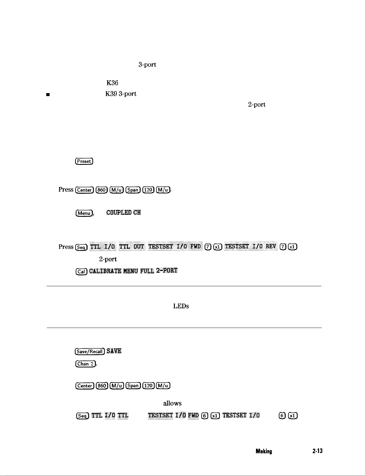
Required Equipment

Characterizing a duplexer requires that the test signals between the analyzer (a Z-port instrument) and the duplexer (a

3-port

device) are routed correctly. This example uses one of

the following adapters to perform this function:

n HP 87533 Option

HP 87533 Option

You must also have a set of calibration standards for performing a full

K36

duplexer test adapter

K39 3-port

test adapter

2-port

calibration on

your test set up.

Procedure for Characterizing a Duplexer

1. Connect the test adapter to the analyzer according to the instructions for your particular model. Connect any test fixture or cables to the duplexer test adapter.

2. Press

IPreset)

3. Set up the stimulus parameters for channel 1 (center/span frequencies, power level, IF

bandwidth). This example uses a span of 120 MHz centered at 860 MHz.

4. Uncouple the primary channels from each other: Press

set

CDUPLEB @I

to OFF.

(This is necessary in order to set the test set I/O independently for each channel.)

5. Set up control of the test adapter so that channel 1 is TX:

6. Perform a full Press

Cal) $XLfBIkATE l#$NJ FTJLL 2-PORT

2-port

calibration on channel 1. (Refer to chapter 5, if necessary.)

, and follow the instructions to complete the

calibration.

Note

Make sure you connect the standards to the TX port of the test adapter (or a

cable attached to it) for the FORWARD calibration and to the Ant port for the

REVERSE calibration. The

LEDs

on the test adapter indicate the active ports:

a brightly lit LED indicates the source port; a dimly lit port indicates the input

port; an unlit LED indicates no connection.

7. When the calibration has been completed, save the instrument state:

Press

@ave/Recall] SAVJJ

Press

@iGTj.

STATE

9. Set up channel 2 for the same stimulus parameters as channel 1.

Press

1Center) (%ZJ (iGJJ (%jZJ (ZGJ cM_II?)

10. Set up control of the test adapter so that channel 2 is measuring the receive path of the duplexer: (Uncoupling the channels

Press

lGi) TTL I/Q Tn,

OUT

allows

T]ESTSET

a different calibration for each signal path.)

If0 FUI&J

Ixl)

TESTSET

IllI

REV @

Ixl)

Making Measurements 2-13

11. Perform a full Press

(ETJ ~~~~~~

....... ..................... i

2-port

calibration on channel 2:

...................... ...... .............. ............... ........... ........... ....... .......

HIT& ‘I’LL ,3-PIIRT

Note

Make sure you connect the calibration standards to the Rx port of the test adapter (or a cable attached to it) for the FORWARD calibration, and the Antenna port for the REVERSE calibration.

12. When the calibration has been completed, save this state in the analyzer:

,. ,,,

13. Connect the DUT to the test adapter.

14. Enable both auxiliary channels 3 and 4:

16. Set the measurement parameters (channel 1 should be active):

.y...

Press

.g%~.

.i .:..: /

. . . .

This is the transmission of the Tx-to-Ant path.

..,.: :..

<.:.

b. Press (Chan] to activate channel 3, press

:@,%,;

This is the reflection at the TX port.

;

Press

(m)

#&,

>>>>.>,.>>>..

.,,,., /

This is the transmission of the Ant-to-Rx path.

Press @iGZ] to activate channel 4, press

This is the reflection at the Rx port.

The display will be similar to Figure 2-7.

I&$

2-14 Making Measurements

CHl CH2

s21 s12

LOG LOG

10 dB/REF

dB/REF

-40

dB dE

5 Aug 1998

13:lO:ll

Ref

1: FWO

Sll IA/R)

PRm Cot-

t T

CHl/CH3 CH2/CH4

zi;

I I

CENTER CENTER

dB/REF

10 dB/REF

860.000 000

MHz MHz SPFIN

Figure

2-7. Duplexer Measurement

SP4N 120.000 000

120.000 000

MHz MHz

Trans: FWD

521

Trans.: REV

512 <A/R)

Ref 1: REV

S22 <B/R)

ANALOG IN Aux Input

CONVERSION

<B/R>

COFFI

INPUT

PORTS

Normally, a the displayed trace. For faster active display

2-port

calibration requires a forward and reverse sweep to finish before updating

(Sll

and

timing,

S21

for channel 1 in this case) to update more often than the unused

it is possible to set the number of sweeps for the

parameters. In this example we choose 8 updates of the forward parameters to 1 update of the reverse in channel 1, and 8 updates of the reverse to 1 update of the forward in channel 2 (where the active parameters are

S22

and

S12).

Making Measurements

2-l

Using Analyzer Display Markers

The analyzer markers provide numerical readout of trace data. You can control the marker search, the statistical functions, and the capability for quickly changing stimulus parameters with markers, from the

Markers have a stimulus value (the x-axis value in a Cartesian format) and a response value (the y-axis value in a Cartesian format). In a polar or Smith chart format, the second part of a complex data pair is also provided as an auxiliary response value. When you switch on a marker, and no other function is active, the analyzer shows the marker stimulus value in the active entry area. You can control the marker with the front panel knob, the step keys, or the front panel numeric keypad.

If you activate both data and memory traces, the marker values apply to the data trace.

n If you activate only the memory trace, the marker values apply to the memory trace. n If you activate a memory math function (data/memory or data-memory), the marker values

apply to the trace resulting from the memory math function.

($GZZZJ

key.

The examples in this section are shown with

‘Ib

Use Continuous and Discrete Markers

Alter

measurement results

The analyzer can either place markers on discrete measured points, or move the markers continuously along a trace by interpolating the data value between measured points.

Choose

,:; ;,,,:.;..;.; .::z

~~~~~~~~~~~~

.:.;.:.:..:::::::t.::.:::::.:::::::

;.:>y;;; ,<<<;;;. .“’ : ,,,, .,.;_ ,.,.....

AC%+%.::.2 . . . . . i . . . . . . . . . .

<.i:

..:.................:

:::..:..:.::

you want the analyzer to place markers

at my

p&t

i;;,;.;z;T;~,y,;;.’

on the trace, by interpolating between measured points. This default mode allows you to conveniently obtain round numbers for the stimulus value.

. . . .

Choose ~,~~~~~~~~~~~

. . . . .

....~~~....

..........

. ..,.........

t.... :Y;.;.:r.::::

.._

z.:

:::;:..>.-:

if you

.....>.i

wit

the analyzer to place markers only on measured

trace points determined by the stimulus settings. This may be the best mode to use with automated testing, using a computer or test sequencing because the analyzer does not interpolate between measured points.

.;;

5::

Note

Using .~~~~~:~~~

. . . . . . .

..T . . . . . . . . . ... . . .:::.>;.::..~

.C<<<<.<.) ,: <::<<<<<, .I;;.;;;/ -:. .~~ .~~ .:::.

. . . . . . . . . . . . . . w2.i . . . . . . . . . . . . ,.,..

,.,., ..,., ,../ . . .

:.::

:.x.::..::<< ,..... .: ......:.::.;~~~~~:.:

m &o

.,.. s.w>:

afled marker

~a&

positio~g

functions when the value entered in a search or positioning function does not

exist as a measurement point.

2-16

Making Measurements

‘lb

Activate Display Markers

switch on marker 1 and make it the active marker, press:

The active marker appears on the analyzer display as V. The active marker stimulus value is displayed in the active entry area. You can modify the stimulus value of the active marker, using the front panel knob or numerical keypad. All of the marker response and stimulus

values

are displayed in the upper right comer of the display.

Figure 2-8. Active Marker Control

‘#lb

switch on the corresponding marker and make it the active marker, press:

All of the markers, other than the active marker, become inactive and are represented on the

analyzer display as A.

Figure 2-9. Active and Inactive

switch off all of the markers, press:

Markers

Making Measurements

2-l

Move Marker Information off of the Grids

If marker information obscures the display traces, you can turn off the softkey menu and move the marker information off of the display traces and into the softkey menu area. Pressing the

backspace key @ performs this function. This is a toggle function of the backspace key. That

is, pressing &) alternately hides and restores the current softkey menu. The softkey menu is also restored when you press any softkey or a hardkey which leads to a menu.

1. Set up a four-graticule display as described in “Using the Four-Parameter Display Mode.”

2. Activate four markers: Press

Note

Observe that the markers appear on all of the grids. F activate markers on

individual

UNCOUPLED.

press

grids, press 0))

@iGiG),

[jGi&J

Then, activate the channel:m~~~~~~~

1 2 3 4

~~~~~~..~~.,

i . ../. _:

then select the markers for that channel.

set ;f#&&&

wish to :K;2AL.AAiers,

3. Turn off the softkey menu and move the marker information off of the grids:

The display will be similar to Figure 2-10.

2 Sep 1998 12:12:09

CHl LO8 Sll

4:-1.4031

PRI

.5 dB/ REF

151.509500

-2

MHz

CHl

Markers

:-I.0229 dB

.88200

:-3.1809

.46850

‘-3.1489

.97600

MHz

CH2

LOG

s21

4:-69.132 dB 151.509 500 MHz

PRm

dB/

REF -50

Press

CH2

Markers

l:-75.710

116.88200 2:-23.481

129.46850 MHz

3:-23.407

139.97600 MHz

MHz

CENTR 134.000 MHz SPAN 45.000 MHz CENTR 134.000 MHz SPAN 45000 MHz

Lo8

4:-70.257

CENTR 134.000

10 dB

dB/

151.509500 REF -50 dB MHz

'-75.661

-22.928

MHz

SPAN 45.000 MHz CENTR 134.000 MHz SPAN 45000 MHz

L0G

4:-2.1132 .5

dB dB/

151.509 500

REF -2.5

MHz

Figure 2-10. Marker Information Moved into the Softkey Menu Area

CH4

Markers

S-1.7005

116.88200

2-3.8129

129.46850 MHz

3:-3.9114

139.97600 MHz

MHz

4. Restore the softkey menu and move the marker information back onto the graticules: Press

The display will be similar to Figure 2- 11.

CHI

LO8 5 dB/’ REF -2

4:-1.4066 dB

Sll

151.509 500 MHz

CHI l:-1.0169 dB

‘9

CENTR 134.000 MHz SPAN 45.000 MHz

10 dB/

zi: LDG

4:-71.254

REF -50

dB 151.509 500 MHz

I I I I I I I I I I

/-ICI3

Markers

.88200

MHz

:-3.1934

.46850

‘-3.1585

-97600 MHz

6.88200 MHz

.97600

MHz

Markers

MHz

2 Sep 1998

CH2

LOG 10

521

4:-69.313 dB 151.509 500

PRm

12:09:

dB/

REF -50 dB

CENTR

134.000 MHz SPAN 45000 MHz

LDG 4:-2.114i

5 dB

dB/REF

MHz

151.509 -2.5 500 dB MHz

37 dB 0 MHz

0 MHz

MARKER

all

OFF

MODE

CENTR 134.000 MHz SPAN 45.000 MHz

Figure 2-11.

You can also restore the

or pressing a

softkey

softkey.

MKR

Marker

CENTR

134.000 MHz SPAN

45000

MHz

Information on the Graticules

menu by pressing a hardkey which opens a menu (such as

ZERO

Making Measurements

248

Use Delta (A) Markers

This is a relative mode, where the marker values show the position of the active marker relative to the delta reference marker. You can switch on the delta mode by

dehning

one of the

five markers as the delta reference.

Press LMarker_) :A. ~~~~~

:& I#F=:i to make marker 1 a reference marker.

2. To move marker 1 to any point that you want to reference:

q turn the front panel knob,

q enter the frequency value (relative to the reference marker) on the numeric keypad.

Press

~I$A&$#$

and move marker 2 to any position that you want to measure in reference

to marker 1.

Figure

2-12.

Marker

1 as the Reference Marker

4. lb change the reference marker to marker 2, press:

~~~~~~,,~~~~ ~~~~

L.. .,,, :.~.k

.: a:.:: T..Y :::.21..

Activate a Fixed Marker

When a reference marker is position. The analyzer allows you to activate a

h:: :. . . . . . . . . . . . . ::.:.::.:.: . . . . =:A..

fixed,

it does not rely on a current trace to maintain its fixed

fIxed

marker with one of the following key

sequences:

. . . .

.~~~~~

.:...i.:

i....... / /.

. . . . . . . . . .

..>.i i. ~.......-i.i~.;:...;::.:..:::.

.:...,.,

. . ;

..,.

. . . .

/.,;,

~~~~~~~~~~~~(

.<<<......

~:::<+::<....~.

..i ..:i

<<.:... .:::..

.:.::<.:..

2-20 Making Measurements

Using

the

AREF=AFIXED MHR Key to Activate a

F’ixed

Reference Marker

1. To set the frequency value of a hxed marker that appears on the analyzer display, press: (Marker_)

AMODE

AREF=AFIXED

MKR

AMODE

MENU FIXED MKR POSITION

FIXED MKR STIMULUS and turn the front panel knob or enter a value from the front panel

keypad. The marker is shown on the display as a small delta (A), smaller than the inactive marker

triangles.

2. To set the response value

(dB)

of a

fixed

marker, press:

FIXED MKR VALUE and turn the front panel knob or enter a value from the front panel

keypad. In a Cartesian format, the setting is the y-axis value. In polar or Smith chart format, with a

magnitude/phase marker, a real/imaginary marker, an R + jX marker, or a G + jB marker, the setting applies to the first part of the complex data pair. (Fixed marker response values are always uncoupled in the two channels.)

3. To set the auxiliary response value of a fixed marker when you are viewing a polar or Smith format, press:

FIXED

MKR !UX

VALUE and turn the front panel knob or enter a value from the front panel

keypad.

This value is the second part of complex data pair, and applies to a magnitude/phase marker,

real/iaginary

marker, an R+ jX marker, or a G+jB marker. (Fixed marker auxiliary

response values are always uncoupled in the two channels.)

Figure 2-13.

Example of a Fixed Reference Marker Using

&REF~AFXXED

MKR

Making Measurements 2-21

Using the

MK&.$$i!%Cl

Key to Activate a Fixed Reference Marker

::9.:3

Marker zero enters the position of the active marker as the A reference position. Alternatively,

you can specify the

point with

.jZU$D HE~,.PfEUTXO~

. Marker zero is canceled by

fixed

switching delta mode off.

1. To place marker 1 at a point that you would like to reference, press:

(JGiG] and turn the front panel knob or enter a value from the front panel keypad.

2. lb measure values along the measurement data trace, relative to the reference point that you set in the previous step, press:

i ,. ;” :;#&&2Jj2$&

.,.,.,.,

and turn the front panel knob or enter a

value

from the front panel keypad.

3. To move the reference position, press: . .

.:..

. . .

.,,, /,.., ,..’

~.~~~~.~;~,~~

. . . . . . .

: ..,... :; ..:.. :.:.:.:z ./

*,...

. . . . . . . . . . . . .

~~~~~~~;~~~~~~~~amr- $“xm m..c$TxaJJ$ ad turn the front panel knob

...“’

::i

:..,... :::....;>.I;::

...: ..:.......:...

,,,... :..:.:.:..:...p . ..i

. . .

..:...

. . . . . . . . . . . . .

. . .../

;.d:

or enter a value from the front panel keypad.

Figure 2-14. Example of a Fixed Reference

2-22 Making Measurements

CEIITER 10.230

000

CI~JO

GH:

SPAIJ

I.000 000 @On GHz

.~.~.:,~,,:~~~.~ ,.z

Marker

Using

&@J$I#&

.~~......,.;..,...

,....;..;:;

_;;;;;.i.i._

. . .

Couple and Uncouple Display Markers

At a preset state, the markers have the same stimulus values on each channel, but they can be uncoupled so that each channel has independent

F?ess (j-1

&&&$$#fJfi& $IEMlJ

i /i ..A..

>;;; ;:

and select from the following keys:

markers.

CHI

PRm

b-J

CENTER IO.240

Choose

~~~~~~~~~~~~

if you want the analyzer to couple the marker stimulus values

for the two display channels.

,.~ ., .,.,. ,. .,.,.

. . .

.,. .,.

Choose ~~~~.:~.~~~~~~~~

. .

..z... . ..i....

,..,..,. _ _ _ ,.

.,.

.;.........*

,. ..;

. . . . ..i./.

..,.., /,.., ., ,.

you want

the analyzer to uncouple

the marker sth&ls

values for the two display channels. This allows you to control the marker stimulus values independently for each channel.

log MAG

I I

lcsg

MA6 10de/ REF

10 de/ REF

I/” I I” I

I I I

000000 GHz

-30 de

-29.92

SPAN 2.500

-: 77.54Q dE

I I

dEi

3X:

77.549

de log

y.-

000

00!1 GHz ;TART GHz

log MAG

e e

t I

MA6

PRK!

10 de/

I I

REF

-30 de

I I I

de,/

REF

-29.92

STUP 11.490

~69.4qij dE

~22.23

000 GHz

dE_

Figure 2-15. Example of Coupled and Uncoupled

Biarkers

To Use Polar Format Markers

The analyzer can display the marker

. . . “:

;.&~#EJ!E% .,

.._..........................................

.,.

.z~:zc, .‘“.~:::~

gives

em magnitude and phase, ,;@i& m gives log magnitude md phw,

lin

gives the real value hrst, then the imaginary You can use these markers only when you are viewing a polar display format. (The format is

available from the

Note

(jj)

key.)

For greater accuracy when using markers in the polar format, it is recommended to activate the discrete marker mode. Press

‘~~~~~~~~~, ~~~~~~~~:,

/.........&..

. . . . . . . . . .

. . . . . . . . . . . . .

. . . . . .

..::..z..i:

. .

..A

. . .

..~.....;..~......~;;~~~ ii :..:a ..A.. .A.. ii i i i: i

1. lb access the polar markers, press:

/ ,,,,, ,,

value

as magnitude and phase, or as a real/imaginary pair:

. . . . . . . . . . . . . .

..i i

value.

(jj’

i.:.::

/..

. . . .

~~~~~

.. ..A. i

. . . .

pb677d

i;..:.. ii

Making Measurements 2-23

2. Select the type of polar marker you want from the following choices:

n Choose

LLW ..!!I&

if you want to view the magnitude and the phase of the active marker.

The magnitude values appear in units and the phase values appear in degrees.

n Choose

active marker. The magnitude values appear in

&JG.$LR

if you want to view the logarithmic magnitude and the phase of the

dE3

and the phase values appear in

degrees.

n Choose

.&/X&XK%

if you want to view the real and imaginary pair, where the complex data is separated into its real part and imaginary part. The analyzer shows the marker value the real part (M cos

0),

and the second value is the imaginary part

(M sin 8, where M=magnitude).

Figure

CENTER10240 ouo 000 GHZ SPAN*500

2-16. Example of a Log

Marker

000 000 GHZ

in Polar Format

first

‘It,

Use Smith Chart Markers

The amount of power reflected from a device is directly related to the impedance of the device and the measuring system. Each value of the reflection coefficient (I’) uniquely

defies

a device

impedance; r = 0 only occurs when the device and analyzer impedance are exactly the same.

The reflection coefficient for a short circuit is: I’ = 1 L

180“.

Every other value for I’ also

corresponds uniquely to a complex device impedance, according to the equation:

zL = [( 1 -t r) / (1 - qxzo

where ZL is your test device impedance and Z0 is the measuring system’s characteristic impedance.

Note

Press ~

press (jj,

For greater accuracy when using markers in the Smith chart format, it is recommended to activate the discrete marker mode. Press

~~~,~~~~

.~~~~~~.

~~~~~~~

~~~~~~~~.

.... )(? ..:‘<v~,v

~~~~~~~~~,

““::?y

..: ;

,& y

.S....““,

.<:grz.

turn the front panel knob or

(Marker4

enter a value from the front panel keypad to read the resistive and reactive components of the complex impedance at any point along the trace.

!I’his

is the default Smith chart marker.

The marker annotation tells that the complex impedance is capacitive in the bottom half of

the Smith chart display and is inductive in the top half of the display.

2-24 Making Measurements

Choose

LIN MKR

if you want the analyzer to show the linear magnitude and

the

phase of

the reflection coefficient at the marker.

Choose LOG

MRR

if you want the analyzer to show the logarithmic magnitude and the phase of the reflection coefficient at the active marker. This is useful as a fast method of obtaining a reading of the log magnitude value without changing to log magnitude format.

. Choose

R&m MKR

if you want the analyzer to show the values of the reflection

coefficient at the marker as a real and imaginary pair.

Choose

RtjX MRR

to show the real and imaginary parts of the device impedance at

the marker. Also shown is the equivalent series inductance or capacitance (the series resistance and reactance, in ohms).

. Choose

G+jB MKR

to show the complex admittance values of the active marker in

rectangular form. The active marker values are displayed in terms of conductance (in Siemens), susceptance, and equivalent parallel circuit capacitance or inductance. Siemens are the international unit of admittance and are equivalent to mhos (the inverse of ohms).

Set Measurement Parameters Using Markers

The analyzer allows you to set measurement parameters with the markers, without going through the usual key sequence. You can change certain stimulus and response parameters to make them equal to the current active marker value.

Setting the Start

1. Press

[jGiGEG~

Frequency

and turn the front panel knob or enter a value from the front panel

keypad to position the marker at the value that you want for the start frequency.

Press

MARKER-tSTART

to change the start frequency value to the value of the active marker.

Making Measurements 2-25

CHl 521

lvg

MAG

de/ REF

lL~74.17 dB

MAK(EK 1

8 653150079- ‘Hi:

Figure 2-18. Example of Setting the Start Frequency Using a Marker

Setting the Stop Frequency

FVess (JGGX$

and turn the front panel knob, or enter a value from the front panel

keypad to position the marker at the value that you want for the stop frequency.

Press

, “‘,...”

‘~~~~.

;

to change the stop frequency value to the value of the active marker.

pb678d

CHl S21

PRm

CENTER

log MAG 10 de/ REF

575 036

11.071

GHr

-30 dB

SPAN 4.836

l-1-74.426 de

849 927

GHr

CHl

521

PRm

CENTER 10.319

log MA6

928

10 de/

457

REF

6Hr

Figure 2-19. Example of Setting the Stop Frequency Using a

Setting the Center Frequency

1. Press

(JGZZZJ

and turn the front panel knob, or enter a value from the front panel

keypad to position the marker at the value that you want for the center frequency.

. . . . . . . . . . . . . .

..A /.

Press ~~~~:

..;....;.....................

~,..~;;~..,.;.~...~.~;::

:.: ,....,,:

./ .

. . . . . ii....

..., I:..bi

. . . . . s..w;..;

ii .A......... .

to change the center frequenw

value to the value of the active

marker.

-30 de

SPAN 3.333

Marker

I-:-eo.cio5

556 769

pb679d

GHz

2-26 Making Measurements

_-..

MAiKEK 1

10.21j95 (Hz

MAdKEK b

1 .21 95 G z

I I I /

CENTER e.265

9511 OO(i GHz

Figure

SPAN 6.500

Z-20.

Example of Setting the Center Frequency Using a Marker

000 iJO0

GHi

Setting the Frequency Span

You can the span equal to the spacing between two markers. If you set the center frequency

before you set the frequency span, you will have a better view of the area of interest.

2. Turn the front panel knob or enter a value from the front panel keypad to position the markers where you want the frequency span.

Iterate

between

maker 1 ad marker

by pressing ~#&&&&

ii/:i ..A. i.i'.A.>>.%/

. . . . . .

~~~

respedively,

and turning the front panel knob or entering values from the front panel keypad to position the markers around the center frequency. When finished positioning the markers, make sure that marker 2 is selected as the active marker.

Note

Step 2 cm &-J&

p&o~edusingS~.~~

using this method, it

; .,.,

.,.,

wiIl

not be possible to iterate between marker zero and

i i /r:;...

i .;; 'Z, ". "'Y: t..:<<<;

and ~~~~~,.

/ .,, . .

.*;.;

However,when

marker 1.

ptB80d

Making Measurements 2-27

3il;1e/

REF

44.44

Z-:

13.124

log

MAI,

311

de/ REF

44.44

PRm

CENTER

l(J.215 95rJ OOfl GHi

Figure

Z-21.

SPAN 6.500

0Oi1 000 GHr

Example of Setting the Frequency Span Using

CENTER 10.443

I I / I

4112

355 6Hz SPAN

Markers

Setting the Display Reference Value

1. Press

@E&ZG)

and turn the front panel knob, or enter a value from the front panel keypad to position the marker at the value that you want for the analyzer display reference value.

2. Press

.,...

~~~~~~..

:..::;;.. ..A

. .. ..i.

ii::.:.;

.._. z:...::

to change the reference value to the value of the active marker.

I I

Z.809

204

4.31 I;Hr

pb5Bld

CHl S21CHl S21

PRmPRm

CENTER

CENTER 10.240

Log MkbLog Mkb

10.240

Oiir?

15 de/

REF 39

15 de/

REF 39

000

GHz SPANSPAN 2.500 000 000 GHz

000 GHz

l-:l-:

2.500

000 000

1.650 dB

GHz

MAG

Jn/~-J

CENTER

10.240 000 000

dE/

REF

GHr

Lbg

Figure 2-22. Example of Setting the Reference Value Using a Marker

1.702

SPAN

l-: 1.615

2.500

.-.

' /

000 000

i bG.i\

GHz

2-28 Making Measurements

Setting the Electrical

Delay

This feature adds phase delay to a variation in phase versus frequency, therefore it is only applicable for

Press

ratioed inputs.

(K)

FW33.

2. Press (MarkerFctn) and turn the front panel knob, or enter a value from the front panel keypad to position the marker at a point of interest.

Press

~~~~~~~~.

..i ,.,..,

. . . . . .

..A. :.,.

,,: .: :.:.

to automatically add or subtract enough line length to the receiver

..: ,......

input to compensate for the phase slope at the active marker position. This effectively flattens the phase trace around the active marker. You can use this to measure the electrical length or deviation from linear phase.

Additional electrical delay adjustments are required on devices without constant group delay over the measured frequency span.

$21

CHI

PRm c2

Phase

MAF.KER

10.1

CENTER 10.240000000 6Hz SPAN 3.500000000 GHz

1 GHz

‘I

KEF0D 1 :

11.100 M

300

163.0f1°

OCO GHz

Figure 2-23. Example of Setting the Electrical Delay Using a

Setting the CW Frequency

‘Ib

place a marker at the desired CW frequency, press:

LHl 521

phase

PRm

MARKER

Del

CENTER 10.240 000 000

10.1 2Hz

9Cl

GHz

“I

KFF0D

10.240 000 000

SPAN 7.500 000 000

BIarker

1 :173.57O

M:*

GHr

GHz

You can use this function to set the marker to a gain peak in an amplifier. After pressing

:~~~~~~~~~-, activate a CW frequency power sweep to look at the g& compre&on with

/. . . . . . . .

. . . .

and either turn the front panel knob or enter the value, followed by

;

i..... <.....:.?x

..8..

/..

.;....::.;;:;

. .

..A . . ..a ,.... L;..~;........,....~ii/i

. . . . . . . . . . . . . .:;./: ii =......;;......~...;;

increasing input power.

Making Measurements 2-29

To Search for a Specific Amplitude

These functions place the marker at an amplitude-related point on the trace. If you switch on tracking, the analyzer searches every new trace for the target point.

Searching for the Maximum Amplitude

press Ij) ~~~~~~~~

Press

~~,~~~;~~~.~.

trace.

”

.”

to move the active marker to the

..r..:.:...::..:: ::.:...

to access the marker search menu.

maximum

point on the measurement

Figure 2-24.

Example of Searching for the Maximum Amplitude Using a

Searching for the Minimum Amplitude

Figure 2-25.

Example of Searching for the Minimum Amplitude Using a Marker

Blarker

Searching for a

2.30 Making

Measursments

Target

Amplitude

Press

SEM%Il:. 2’~

,,...........

:.:

to move the active marker to the target point on the measurement

. . . . . . . . . .:

trace.

If you want to change the target amplitude value (default is -3 enter the new value from the front panel keypad.

If you want to search

.,, ,,,:.: ,/

‘SW ‘;Jm

and

for,,multiple

.:.., ;.

.$$J&&#f #$?&jm,.

responses at the target amplitude value, press

,:..::.., ;,..

.:..

dB),

press

X&S&%

and

CHI 521

FRm

leg MAI,

111 dE/ REF

-30

FRm

lc,g

MA6

, ,, / -1.J

CENTER

11,.240

UOCJ O(J(I GHz

Example of Searching for a

Searching for a Bandwidth

The analyzer can automatically calculate and display the -3 dB bandwidth (BW:), center frequency (CENT:), Q, and loss of the device under test at the center frequency. (Q stands for

“quality factor,”

dellned

values are shown in the marker data readout.

SPAN 2.500

as the ratio of a circuit’s resonant frequency to its bandwidth.) These

7,”

irO0 000 GHr

Figure 2-26.

‘beget

CENTER 10.240 OUO

000 GHr

SPAN 2.500

Amplitude Using a Marker

OOil 000 6Hz

pt533d

1. Press

@GiZ)

and turn the front panel knob, or enter a value from the front panel keypad to

place the marker at the center of the filter passband.

3. press ~~~~~~~~:~

,.,... ;. ,,.,.;.: / ., ,,,,

bandpass

or band reject shape on the measurement trace.

4. If you want to change the amplitude value (default is -3

rejectband, press ~~~~~~~~

. . . .

&date

the center sthuh.ls

,::::..:~ ;:..:;:<:yv

. . . . . . . . . . . . . . . ~.wu;;;.;;.;;~.~

.A.. i

. . . . . . . . . . . .

L ii ~.;...:~..>>:..::

enter the

v&e,

new

v&e from the front panel keypad.

bandwidth, ad the Q of

dl3)

that

defines

the passband or

Making Measurements 231

Figure 2-27.

CE,,,EH 1” Z4il 0”” 00” OH:

Example of Searching for a Bandwidth

SPA,! 1

OClll b”,1

Trackiug the Amplitude that You Are Searching

‘OCi GHZ

using

Markers

1. Set up an amplitude search by following one of the previous procedures in Specific Amplitude.

Press [-FctnJ ~~~~~~ ~~~~~~~~;~~,, to track the spehfied mpfitude search

..:::.::...

~.~.T./.i .;;;./;:,....~.,....;;..././.

..:

.ss....i

.: .._/

. . . . . . . .

~~.~.~.~.~.

/i..i.i

‘To

Search for a

with every new trace and put the active marker on that point. When tracking is not activated, the analyzer

sweep and the marker remains at same

finds

stimulus

the specified amplitude on the current

value, regardless of changes in the trace

response value with subsequent sweeps.

232 Making Measurements

Calculate the Statistics of the Measurement Data

This function calculates the mean, standard deviation, and peak-to-peak values of the section of the displayed trace between the active marker and the delta reference. If there is no delta reference, the analyzer calculates the statistics for the entire trace.

Press

(j&X$] :~,~;;~~~~~ a

./i

. . . . . . . . . . . . . . . . . . . . . . . . . . . . .

lW?*f. to make marker 1 a reference marker.

2. Move marker 1 to any point that you want to reference:

Turn the front panel knob.

Enter the frequency value on the numeric keypad.

Press

$&I&&$;.&?

and move marker 2 to any position that you want to measure in reference

to marker 1.

4. Press

l$iXXG] ~~~~~~~~~;~ &lT$&&@~

to calculate and view the mean, standard deviation, and peak-to-peak values of the section of the measurement data between the active marker and the delta reference marker.

An application for this feature is to

Gnd

the peak-to-peak value of passband ripple without

searching separately for the maximum and minimum values If you are viewing a measurement in the polar or Smith Chart format, the analyzer

calculates the statistics using the

first

value of the complex pair (magnitude, real part,

resistance, or conductance).

CHI 5-4

P R m

loa MAG

10 de/

REF -30 dE?

2 :

1.117

de.

CENTER

IO.240

000

GHz SPAti

.OOG

000 000

GHz

Figure 2-28. Example Statistics of Measurement Data

Making Measurements 233

_-.

Measuring Magnitude and Insertion Phase Response

The analyzer allows you to make two different measurements simultaneously. You can make these measurements in different formats for the same parameter. For example, you could

measure both the magnitude and phase of transmission. You could also measure two different

parameters

This

measurement example shows you how to measure the

and then how to view the measurement data in the phase format, which provides information

about the phase response.

Measuring the Magnitude Response

1. Connect your test device as shown in Figure 2-29.

(SH

and

SZZ).

maximm

amplitude of a SAW

filter

DEVICE UNDER TEST

Figure 2-29. Device Connections for Measuring a Magnitude Response

2. Press

and choose the measurement settings. For this example, the measurement

parameters are set as follows:

You may also want to select settings for the number of data points, averaging, and IF

bandwidth.

234

Making

Measurements

4. Reconnect your test device.

5. To better view the measurement trace, press:

c-j

&&q:., Km

6. To locate the maximum amplitude of the device response, as shown in Figure 2-30, press:

[m);*.sw

1.:

&k&H: tix-

Example Magnitude Response Measurement

Measuring Insertion Phase Response

‘Ib

view both the magnitude and phase response of the device, as shown in Figure 2-31,

7. press:

@iZ)

The channel 2 portion of Figure 2-31 shows the insertion phase response of the device under test. The analyzer measures and displays phase over the range of

180 O to + 180 O. As phase

changes beyond these values, a sharp 360 O transition occurs in the displayed data.

CENTER IU.240 000 c’oo OH:

*PAP4 2 50” noo 000 GHZ

Figure 2-31. Example Insertion Phase Response Measurement

The phase response shown in Figure 2-32 is undersampled; that is, there is more than

MO0

phase delay between frequency points If the A4 = >

WOO,

incorrect phase and delay

Making Measurements

2-35

information may result. Figure 2-32 shows an example of phase samples with and greater than

180°.

ACTUAL PHASE -

F,E<PONSE

AC#J

less than

HO0

Figure 2-32. Phase Samples

Undersampling may arise when measuring devices with long electrical length. To correct this problem, the frequency span should be reduced, or the number of points increased until Ad is less than

180°

per point. Electrical delay may also be used to compensate for this effect (as

shown in the next example procedure).

236 Making Measurements

Measuring Electrical Length and Phase Distortion

Electrical Length

The analyzers mathematically implement a function similar to the mechanical “line stretchers” of earlier analyzers. This feature simulates a variable length you can add to or remove from the analyzer’s receiver input to compensate for interconnecting cables,

etc.

In this example, the electronic line stretcher measures the electrical length of a

SAW iilter.

Phase Distortion

The analyzers allow you to measure the linearity of the phase shift through a device over a

range of frequencies and the analyzers can express it in two different ways:

n deviation from linear phase

group delay

Measuring Electrical Length

Connect your test device as shown in Figure 2-33.

NETWORK ANALYZER

lossless

transmission line, which

DEVICE UNDER TEST

Figure 2-33. Device Connections for Measuring Electrical Length

Press

1Preset)

and choose the measurement settings. For this example, the measurement settings include reducing the frequency span to eliminate under sampled phase response. Press the following keys as shown:

(jj)(izJ(iiJJ =c@i@

m [K)

!$$#m. @ Lxl] (a @), HP

..~......... ::

.:. ..y,;

““.

jgg&Q.j

. . . . . . ;.... . . . . . . .

.-c.;.i .. . . ;...

...”

8722D)

You may also want to select settings for the number of data points, averaging, and IF bandwidth.

Makine

Mearurrments

2-37

Substitute a thru for the device and perform a response calibration and press:

0~~~~~~~~

Reconnect your test device.

‘lb

better view the measurement trace, press:

..z

,.,., ,.%.

:&f&l

.~~~~~~

‘z!EK

@Eiizz) asp@-. @Ii&E

Notice that in Figure 2-34 the SAW

iilter

under test has considerable phase shift within only a 2 MHz span. Other filters may require a wider frequency span to see the effects of phase shift.

The linearly changing phase is due to the device’s electrical length. You can measure this changing phase by adding electrical length (electrical delay) to compensate for it.

6. To place a marker at the center of the band, press:

(j]

and turn the front panel knob or enter a value from the front panel keypad.

7. To activate the electrical delay function, press:

:: .:,,; ;;;;

_* . .

cF==q

+ ~~~~~~~,

~~~:~~~~~~~~~~.,.,.~.,;,:

This function calculates and adds in the appropriate electrical delay by taking a about the marker, measuring the

Ac$,

and computing the delay as

A+/Afrequency.

flO%

span

238

Makina

Measurements

Press

[sCALE) &&TRK&, ~l&&Y

and turn the front panel knob to increase the

electrical length until you achieve the best flat line, as shown in Figure 2-35. The measurement value that the analyzer displays represents the electrical length of your

device relative to the speed of light in free space. The physical length of your device is related to this value by the propagation velocity of its medium.

Note

Velocity factor is the ratio of the velocity of wave propagation in a coaxial cable to the velocity of wave propagation in free space. Most cables have a relative velocity of about 0.66 the speed in free space. This velocity depends on the relative permittivity of the cable dielectric

velocity factor =

116.

(cp)

You could change the velocity factor to compensate for propagation velocity by pressing

Ical] $@I#& #&&%XiX FA@‘IXJR

,,, i

/.:;.i

(enter the value) (XJ This will help the

;;;

analyzer to accurately calculate the equivalent distance that corresponds to the entered electrical delay.

Figure 2-35.

‘lb

display the electrical length, press:

Example Best Flat Line with Added Electrical

Delay

In this example, there is a large amount of electrical delay due to the long electrical length of the SAW

lUer

under test.

Measuring Phase Distortion

This portion of the example shows you how to measure the linearity of the phase shift over

a range of frequencies. The analyzer allows you to measure this linearity and read it in two different ways: deviation from linear phase, or group delay.

Making Measurements 238

Deviation

From

Linear Phase

By adding electrical length to “flatten out” the phase response, you have removed the linear phase shift through your device. The deviation from linear phase shift through your device is

all that remains.

Follow the procedure in “Measuring Electrical Length.

‘Ib

increase the scale resolution, press:

kz]

,&Kg: #y,

and turn the front panel knob or enter a value from the front panel

To use the marker statistics to measure the maximum peak-to-peak deviation from linear phase, press:

adjust

Activate and

Note

the electrical delay to obtain a minimum peak-to-peak value.

It is possible to use

Amarkers to measure peak-to-peak deviation in only one

portion of the trace, see “lb Calculate the Statistics of the Measurement Data”

located earlier in this chapter.

Figure 2-36. Deviation from Linear Phase Example Measurement

Group Delay

The phase linearity of many devices is specified in terms of group or envelope delay. The analyzers can translate this information into a related parameter, group delay. Group delay is the transmission time through your device under test as a function of frequency. Mathematically, it is the derivative of the phase response which can be approximated by the following ratio.

A4/(360 * AF)

where Ad is the difference in phase at two frequencies separated by commonly

caIled

the “aperture” of the measurement. The analyzer calculates group delay from

Al?

The quantity AF is

its phase response measurements The default aperture is the total frequency span divided by the number of points across the

display (i.e. 201 points or 0.5% of the total span in this example).

1. Continue with the same instrument settings and measurements as in the previous procedure, “Deviation from Linear Phase.”

240 Making Measurements

2. To view the measurement in delay format, as shown in Figure 2-37, press:

3. To activate a marker to measure the group delay at a particular frequency, press:

and turn the front panel knob or enter a value from the front panel keypad.

Figure 2-37. Group Delay Example Measurement

Group delay measurements may require a specific aperture

(Af)

or frequency spacing between

measurement points The phase shift between two adjacent frequency points must be less than

1800,

otherwise incorrect group delay information may result.

4. To vary the effective group delay aperture from

approximately 1% of the frequency spa,

press:

When you increase the aperture, the analyzer removes

minimum aperture (no smoothing) to

~'~~~~~~~~~:~~:~

..v.>..;;;;>

. . . . . . . . .

..i.// i i

fine

grain variations from the

response. It is critical that you specify the group delay aperture when you compare group delay measurements

CENTER

,134 00” 000 GHi

SPAN

cl”2 00” 000 WI:

Figure 2-38. Group Delay Example Measurement with Smoothing

Making Measurements 241

‘lb

increase the effective group delay aperture, by increasing the number of measurement

points over which the analyzer calculates the group delay, press:

As the aperture is increased, the “smoothness” of the trace improves markedly, but at the expense of

measurement

detail.

Group Delay Example Measurement with Smoothing Aperture Increased

242 Making Measurements

Tbsting

a Device with Limit Lines

Limit testing is a measurement technique that compares measurement data to constraints that you define. Depending on the results of this comparison, the analyzer will indicate if your device either passes or fails the test.

Limit testing is implemented by creating individual flat, sloping, and single point limit lines on the analyzer display. When combined, these lines represent the performance parameters for your device under test. The limit lines created on each measurement channel are independent of each other.

This example measurement shows you how to test a

bandpass filter using the following

procedures:

creating flat limit lines

creating sloping limit lines

creating single point limit lines

editing limit segments

n running a limit test

Setting Up the Measurement Parameters

1. Connect your test device as shown in Figure

Z-40.

DEVICE UNDER TEST

2. Press

Figure 2-40. Connections for

and choose the measurement settings For this example, the measurement

SAW

Filter Example Measurement

settings are as follows:

You may also want to select settings for the number of data points, power, averaging, and IF bandwidth.

3. Substitute a thru for the device and perform a response calibration by pressing:

Making Measurements 243

pb69d

4. Reconnect your test device.

better view the measurement trace, press:

Creating Flat Limit Lines

In this example procedure, the following flat Iimit Iine values are set:

Frequency Range . . . . . . . . . . , . . . . . . . . . . . . . . . . . . . . . . . . . . . . . . . . . . . . . . . . . . . . . . . . . . . . . . Power Range

10.11 GHz to 10.37 GHz . . . . . . . . . . . . . . . . . . . . . . . . . . . . . . . . . . . . . . . . . . . . . , . . . . . . . -1.4 dB to -7.4 dB

GHz

to 9.75 GHz . . . . . . . . . . . . , . . . . . . . . . . . . . , . . . . . . . . . . . . . . . . . . . . . . . . . . . . . . . .

10.8

GHz

to 11.48 GHz..

.~.............,........,.............,..............

120 dB to -45 dB

-120 dB to -45

Note

access the

To create a new Iimit

The minimum value for measured data is -200

limits

menu and activate the Iimit

line,

press:

lines,

press:

dB.

The analyzer generates a new segment that appears on the center of the display. determining the value of the new segment, marker 1 also appears on the display.

‘ib

specify the stimuius value, test limits (upper and lower), and the iimit type of the iimit

line’s

starting point, press:

‘Ib

aid in

“- ....... : I,:.:.:,,......, ;...:.:.:.:.:.:.:.:.:.:.:.:.:.:.;.... ;.::: ,.

~~~~~~~~~~ ;,;;,~,;,;,:,~,,~~,,

,; ,,,, ;: ,/ :.:.:;;.;,.,;;,;‘: i..,.,.,.,.,.,.,.,.,.,,_,.,.,.,,,....

,~~~~~~~~

ii ..::....

. . . . . . . . . . . . . . . . . . . . . . . ..~.~...~.~~~.... . . . . . . . . . i ..,......... w;;....;

.,..” :.::::::.

.., .,. .,.. .,..,..,.,.. _

//_

This would correspond to a test specification of -4.4 f3

4. To define the Iimit as a flat

,~~~~~~~ ~~~~~,~~,:, ~~

__i_

244

Making Measurements

...i;;;.~~.~~.:.:.,. .:;.; .././.... /..

::<.<:..:

(--4.4) Ixl)

~.~ ;.,.

p-J Lxl]

line,

press:

. . . .

-.. ..::;~...:.::..~:...::.~:......

dI3.

5. To terminate the flat line segment by establishing a single point limit, press:

iFKm?&g$

. . . .

DOHE

//i /:..

:..

i. ..:i..

/.i

:4&&y

. . . . .

,,,,.........,.,

L1D.37) (ZJYj

&g-;ET” *g. i$~#&y$ ggggff #$TJQg

Figure 2-41 shows the flat limit lines that you have just created with the following parameters:

stimulus from 10.11

upper limit of -1.4

n lower limit of -7.4

GHz

to 10.37

GHz

.-..

‘lb

create a

limit

line that tests the high side of the bandpass

lilter,

press:

Creating a Sloping Limit Line

This example procedure shows you how to make limits that test the shape factor of a SAW filter. The following limits are set:

Frequency Range . . . . . . . . . . . . . . . . . . . . . . . . . . . . . . . . . . . . . . . . . . . . . . . . . . . . . . . . . . . . . . . . . Power Range

9.7

GHz to 10 GHz . . . . . . . . . . . . . . . . . . . . . . . . . . . . . . . . , . . . . . . . . . . . . . . . . . . . . . . . . . . . . -45

10.48

GHz

to 10.8

’

access the limits menu and activate the limit lines, press:

GHz

. . . . . . . . . . . . . . . . . . . . . . . . . . . . . . . . . . . . . . . . . . . . . . . . . . . . . . . .

dE3

to +4 dB

+4 dB

to -45

2.46 Making Measurements

3. To terminate the lines and create a sloping limit line, press:

4. To establish the start frequency and limits for a sloping limit line that tests the high side of the

filter,

press:

Figure 2-43. Sloping Limit Lines

Making Measurements 247

Creating Single Point Limits

In this example procedure, the following

from +4 dB to -2 dB at 10.15 from +4 dB to -2 dB at 10.33

1. To access the

2. lb designate a

downward pointing, indicating the upper test Iimit

upward pointing, indicating the lower test Iimit

limits

menu and activate the Iimit

single

point Iimit

GHz

En-tits

line,

as shown in

are set:

lines,

F’igure

press:

2-44, you must

dellne

two pointers;

248

Makiq

Measurements

Figure 2-44. Example Single Points Limit Line

Editing Limit Segments

This example shows you how to edit the upper limit of a limit line.

1. To access the limits menu and activate the limit lines, press:

2. To move the pointer symbol

(>)

on the analyzer display to the segment you wish to modify,

press:

%&&’

. . . . . .: . . . . . . . . . . . .

3. To change the upper limit (for example, -20) of a limit line, press:

:,&&g:,, ~~~~~:~~:~, L-20) Lxl] g#

and enter the segment number followed by

..-..i..~...

Lxl]

;.,, ,,,, ,...T.

Deleting Limit Segments

1. To access the limits menu and activate the limit lines, press:

‘lb

move the pointer symbol

press:

,&$@~or@repeate~y

OR .;;;;/; fl,:

~$@%&J@

. .

,..........

I::...:.~~.:.~;.;;;.-i..r

.<:.<<.

and enter the segment number followed by

. . . . . .

3. lb delete the segment that you have selected with the pointer symbol, press:

~~~

.........

. . .

..~~~~..~.....~.;;..;;~.;;..~

(>)

on the analyzer display to the segment you wish to delete,

Making Measurements 248

Running a Limit Test

1. To access the limits menu and activate the limit lines, press:

Reviewing the Limit Line Segments

The limit table data that you have previously entered is shown on the analyzer display.

2. To verify that each segment in your

3. To modify an incorrect entry, refer to the “Editing

limits

table is correct, review the entries by pressing:

Limit

Segments” procedure, located

earlier in this section.

Activating the Limit

l&t

4. To activate the limit test and the beep fall indicator, press:

Note

&lecting

the beep fail ~&&or

:6&J; ~~~~~~~~. is optional

and a add

approximately 50 ms of sweep cycle time. Because the limit test will still work

if the me lines ue off, selecting ~~~~~~~~~~~~~:~~ is alSo optional.

..:.:.

.::..v

. . . . . . . .

.;.;z:

,...i .

..m 2

The limit test results appear on the right side on the analyzer display. The analyzer indicates whether the filter passes or fails the dellned limit test:

The message FAIL will appear on the right side of the display if the limit test fails

0 me analyzer

The analyzer alternates a red trace where the measurement trace is out of

Tl’L

beeps if the mt test fails ad if ~~~~~~~~~.~~I~~~

signal on the rear panel BNC connector

.T:.::,.y,.'.:.~ ') / "' ...

“LIMIT

. . . . . . . . . . . .

.._...

been s&&d.

limits.

TEST” provides a pass/fail (5 V/O

indication of the limit test results

260

Making Measurements

Offsetting Limit Lines

The limit offset functions allow you to adjust the limit lines to the frequency and output level

of your device. For example, you could apply the stimulus offset feature for testing tunable filters. Or, you could apply the amplitude offset feature for testing variable attenuators, or

passband

This example shows you the offset feature and the limit test failure indications that can appear

on the analyzer display.

ripple in filters with variable loss.

1. To offset all of the segments in the

limit

table by a llxed frequency, (for example, 50 MHz),

press:

The analyzer beeps and a FAIL notation appears on the analyzer display, as shown in

Figure

2-45.

Figure

2-45. Example Stimulus Offset of Limit Lines

return to 0 Hz offset, press:

,. :~-~:.::~,::~~;-:; ~~~~~~~~~~~~~~ @ lxlJ

”

.c,

.~......~.~.........~~..~.~.~

‘..~~~..~~“,,“:~..:.

~.~.~...;;;....::.~...

.,.

..z ::..

3. To offset all of the segments in the limit table by a fixed amplitude, press:

~~~~~~~~o~

..:t~:~~~..:.~~~~~~~.;;;,.~,~,.,:;~:

_ _ _. .,.;,,.

,,. ,.,..

.,,,, /*

,.,,. /

. . . . . . . . . i . . ii . . . . . . . . . . . . . . . . . . . . . . . .../..

The analyzer beeps and a FAIL notation appears on the analyzer display.

Making Measurements

2-51

Measuring Gain Compression

Gain compression occurs when the input power of an amplifier is increased to a level that reduces the gain of the amplifier and causes a nonlinear increase in output power. The point at which the gain is reduced by 1 will vary with frequency, so it is necessary to

the frequency band. Once that point is identified, you can perform a power sweep of that CW frequency to measure

the input power at which the 1 compression. The following steps provide detailed instruction on how to apply various features of the analyzer to accomplish these measurements.

is called the 1

dI3

compression occurs and the absolute power out (in

dl3

compression point. The gain compression

find

the worst case point of gain compression in

dBm)

Input Power (dBm)

Figure 2-46. Diagram of Gain Compression

Note

1. Set up the stimulus and response parameters for your amplifier under test. To reduce the effect of noise on the trace, press:

2. Perform the desired error correction procedure. Refer to Chapter 5, “Optimizing Measurement Results,” for instructions on how to make a measurement correction.

3. Hook up the amplifier under test.

produce a normalized trace that represents gain compression, perform either step 5 or

step 6. Step 6 is optional

If the default output power of your analyzer is not high enough to force the amplifier under test into compression, then the following procedure may have to be performed with

the

addition of Option 007 or Option 085. Refer to “Hi

Power Measurements” for information on using Option 085.

2-62

Making Measurements

Agilent 8720D User’s Guide

Specifications and Main Features

Frequently Asked Questions

User Manual

Contacting Agilent

Where to Look for More Information

Analyzer Description

Front Panel Features

Analyzer Display

Rear Panel Features and Connectors

Analyzer Options Available

Service and Support Options

Making Measurements

Where to Look for More Information

Principles of Microwave Connector Care

Basic Measurement Sequence and Example

Basic Measurement Sequence

Using the Display Functions

Using the Four-Parameter Display

Four-Parameter Display and Calibration

Characterizing a Duplexer

Required Equipment

Procedure for Characterizing a Duplexer

Using Analyzer Display Markers

To Use Polar Format Markers

To Search for a Specific Amplitude

Measuring Magnitude and Insertion Phase Response

Measuring the Magnitude Response

Measuring Insertion Phase Response

Measuring Electrical Length and Phase Distortion

Measuring Electrical Length

Measuring Phase Distortion

Setting Up the Measurement Parameters

Creating Flat Limit Lines

Creating a Sloping Limit Line

Creating Single Point Limits

Editing Limit Segments

Deleting Limit Segments

Running a Limit Test

Offsetting Limit Lines

Measuring Gain Compression