Agilent 8712ET User Manual

Download

User’s Guide

Agilent Technologies

8712ET and 8714ET

RF Network Analyzers

Part No. 08714-90011

Printed in USA

Print Date: June 2000

Supersedes: October 1999

Notice

Softkey

The information contained in this document is subject to change without notice. Agilent Technologies makes no warranty of any kind with regard to this material, including but not limited to, the implied warranties of merchantability and ﬁtness for a particular purpose. Agilent Technologies shall not be liable for errors contained herein or for incidental or consequential damages in connection with the furnishing, performance, or use of this material.

Key Conventions

This manual uses the following conventions:

FRONT PANEL KEY

This represents a key physically located on the instrument (a “hardkey”).

This indicates a “softkey,” a key whose label is determined by the instrument’s ﬁrmware, and is displayed on the right side of the instrument’s screen next to the eight unlabeled keys.

Screen Text

This indicates text displayed on the instrument’s screen.

Safety Information

For safety and regulatory information see Chapter 10, “Safety and

Regulatory Information.” For warranty and assistance information see Chapter 9, “Speciﬁcations.”

Firmware Revision

This manual documents analyzers with ﬁrmware revisions E.06.00 and above.

ii ET User’s Guide

Acknowledgments

Lotus® 1-2-3® are U.S. registered trademarks of Lotus Development Corporation.

Windows, Word97, and Excel97 are registered trademarks of Microsoft Corp.

Portions of the software include source code from the Info–ZIP group. This code is freely available on the Internet by anonymous ftp asftp.uu.net:/pub/archiving/zip/unzip51/.tar.Z, and from CompuServe asunz51.zip in the IBMPRO forum, library 10, (data compression).

ET User’s Guide iii

Introducing the Analyzer

The Agilent Technologies 8712ET and 8714ET are easy-to-use RF network analyzers optimized for production measurements of reﬂection and transmission parameters. The instrument integrates an RF synthesized source, transmission/reﬂection test set, multi-mode receivers, and display in one compact box.

The source features 1 Hz resolution, 40 ms (or faster) sweep time, and up to +16 dBm output power.

The three-channel, dual mode receivers provide dynamic range of greater than 100 dB in narrowband-detection measurement mode. For measurements of frequency-translating devices, the network analyzer features broadband internal detectors and external detector inputs. The receivers incorporate digital signal processing and microprocessor control to speed operation and measurement throughput.

Two independent measurement channels and a large display show the measured results of one or two receiver channels in several user-selectable formats. An external VGA monitor can be connected to the rear panel for enhanced measurement viewing in color.

Measurement functions are selected with front panel hardkey and softkey menus. Measurements can be printed or plotted directly with a compatible peripheral. Instrument states can be saved to the internal ﬂoppy disk, internal non-volatile memory, or internal volatile memory. Built-in service diagnostics are available to simplify troubleshooting procedures

Measurement calibrations and data averaging provide performance improvement and ﬂexibility. Measurement calibrations consist of normalizing data, utilizing the internal factory calibration, or calibrating with external standards. Measurement calibration reduces errors associated with crosstalk, directivity, frequency response, and source match. Refer to Chapter 9, “Speciﬁcations,” for error correction speciﬁcations.

iv ET User’s Guide

How to Use This Guide

The ﬁrst 6 chapters of this guide explain how to perform measurements, calibrate the instrument, and use the most common instrument functions.

Chapters 7 through 11 are reference material. Use these chapters to look up information such as front panel features, speciﬁc key functions, and speciﬁcations.

ET User’s Guide v

8712ET and 8714ET Network Analyzer Documentation Map

The CDROM provides the contents of all of the documents listed below.

The User’s Guide shows how to make measurements, explains commonly-used features, and tells you how to get the most performance from the analyzer.

The LAN Interface User’s Guide Supplement shows how to use a local area network (LAN) for programming and remote operation of the analyzer.

The Automating Measurements User’s Guide Supplement provides information on how to conﬁgure and control test systems for automation of test processes.

The Programmer’s Guide provides programming information including GPIB and SCPI command references, as well as short programming examples.

The Example Programs Guide provides a tutorial introduction using BASIC programming examples to demonstrate the remote operation of the analyzer

vi ET User’s Guide

The Service Guide provides the information needed to adjust, troubleshoot, repair , and verify analyzer conformance to published speciﬁcations.

The HP Instrument BASIC User’s Handbook describes programming and interfacing techniques using HP Instrument BASIC, and includes a language reference.

The HP Instrument BASIC User’s Handbook Supplement shows how to use HP Instrument BASIC to program the analyzer.

The Option 100 Fault Location and Structural Return Loss Measurements User’s Guide Supplement provides theory and measurement examples for making fault location and SRL measurements. (Shipped only with Option 100 analyzers.)

The CATV Quick Start Guide provides abbreviated instructions for testing the quality of coaxial cables. (Shipped only with Option 100 analyzers.)

The Cellular Antenna Quick Start Guide provides abbreviated instructions for verifying the performance of cellular antenna systems. (Shipped only with Option 100 analyzers.)

ET User’s Guide vii

Contents

1. Installing the Analyzer

Introduction . . . . . . . . . . . . . . . . . . . . . . . . . . . . . . . . . . . . . . . . . . . . . . . . . . . . . . . . . . . 1-2

Step 1. Check the Shipment . . . . . . . . . . . . . . . . . . . . . . . . . . . . . . . . . . . . . . . . . . . . . . 1-3

Step 2. Meet Electrical and Environmental Requirements. . . . . . . . . . . . . . . . . . . . . . 1-4

Step 3. Check the Analyzer Operation . . . . . . . . . . . . . . . . . . . . . . . . . . . . . . . . . . . . . . 1-9

Step 4. Conﬁgure the Analyzer. . . . . . . . . . . . . . . . . . . . . . . . . . . . . . . . . . . . . . . . . . .1-10

Connecting Peripherals and Controllers. . . . . . . . . . . . . . . . . . . . . . . . . . . . . . . . . . 1-11

Installing the Analyzer in a Rack . . . . . . . . . . . . . . . . . . . . . . . . . . . . . . . . . . . . . . . 1-16

Preventive Maintenance . . . . . . . . . . . . . . . . . . . . . . . . . . . . . . . . . . . . . . . . . . . . . . . . 1-17

Clean the Display. . . . . . . . . . . . . . . . . . . . . . . . . . . . . . . . . . . . . . . . . . . . . . . . . . . . 1-17

Check the RF Front Panel Connectors . . . . . . . . . . . . . . . . . . . . . . . . . . . . . . . . . . . 1-17

2. Getting Started

Introduction . . . . . . . . . . . . . . . . . . . . . . . . . . . . . . . . . . . . . . . . . . . . . . . . . . . . . . . . . . . 2-2

Front Panel Tour . . . . . . . . . . . . . . . . . . . . . . . . . . . . . . . . . . . . . . . . . . . . . . . . . . . . . . . 2-3

Entering Measurement Parameters. . . . . . . . . . . . . . . . . . . . . . . . . . . . . . . . . . . . . . . . 2-4

Presetting the Analyzer . . . . . . . . . . . . . . . . . . . . . . . . . . . . . . . . . . . . . . . . . . . . . . . . 2-5

Entering Frequency Range . . . . . . . . . . . . . . . . . . . . . . . . . . . . . . . . . . . . . . . . . . . . . 2-6

Entering Source Power Level. . . . . . . . . . . . . . . . . . . . . . . . . . . . . . . . . . . . . . . . . . . . 2-6

Scaling the Measurement Trace . . . . . . . . . . . . . . . . . . . . . . . . . . . . . . . . . . . . . . . . . 2-6

Entering Active Measurement Channel and Measurement Type. . . . . . . . . . . . . . .2-7

Viewing Measurement Channels. . . . . . . . . . . . . . . . . . . . . . . . . . . . . . . . . . . . . . . . . 2-8

Performing the Operator's Check . . . . . . . . . . . . . . . . . . . . . . . . . . . . . . . . . . . . . . . . . 2-10

Equipment List. . . . . . . . . . . . . . . . . . . . . . . . . . . . . . . . . . . . . . . . . . . . . . . . . . . . . . 2-10

Make a Transmission Measurement. . . . . . . . . . . . . . . . . . . . . . . . . . . . . . . . . . . . .2-11

Make a Broadband Power Measurement . . . . . . . . . . . . . . . . . . . . . . . . . . . . . . . . . 2-13

Make a Reﬂection Measurement. . . . . . . . . . . . . . . . . . . . . . . . . . . . . . . . . . . . . . . . 2-14

If the Analyzer Fails the Operator's Check. . . . . . . . . . . . . . . . . . . . . . . . . . . . . . . . 2-17

3. Making Measurements

Introduction . . . . . . . . . . . . . . . . . . . . . . . . . . . . . . . . . . . . . . . . . . . . . . . . . . . . . . . . . . . 3-2

Measuring Devices with Your Network Analyzer . . . . . . . . . . . . . . . . . . . . . . . . . . . . . 3-3

Attenuation and Ampliﬁcation in a Measurement Setup . . . . . . . . . . . . . . . . . . . . . 3-8

When to Change the System Impedance. . . . . . . . . . . . . . . . . . . . . . . . . . . . . . . . . . . 3-9

The Typical Measurement Sequence. . . . . . . . . . . . . . . . . . . . . . . . . . . . . . . . . . . . . 3-10

Using the BEGIN Key to Make Measurements. . . . . . . . . . . . . . . . . . . . . . . . . . . . . . 3-11

Contents-ix

Contents

BEGIN Key Overview. . . . . . . . . . . . . . . . . . . . . . . . . . . . . . . . . . . . . . . . . . . . . . . . .3-12

Using the BEGIN Key to Conﬁgure Measurements . . . . . . . . . . . . . . . . . . . . . . . . .3-13

AUTOST Files. . . . . . . . . . . . . . . . . . . . . . . . . . . . . . . . . . . . . . . . . . . . . . . . . . . . . . .3-15

The User BEGIN Function. . . . . . . . . . . . . . . . . . . . . . . . . . . . . . . . . . . . . . . . . . . . .3-15

Measuring Transmission Response. . . . . . . . . . . . . . . . . . . . . . . . . . . . . . . . . . . . . . . .3-16

Enter the Measurement Parameters. . . . . . . . . . . . . . . . . . . . . . . . . . . . . . . . . . . . .3-16

Perform an Enhanced Response Calibration. . . . . . . . . . . . . . . . . . . . . . . . . . . . . . .3-17

Measuring Reﬂection Response. . . . . . . . . . . . . . . . . . . . . . . . . . . . . . . . . . . . . . . . . . .3-33

Enter the Measurement Parameters. . . . . . . . . . . . . . . . . . . . . . . . . . . . . . . . . . . . .3-33

Perform a One-Port Reﬂection Calibration . . . . . . . . . . . . . . . . . . . . . . . . . . . . . . . .3-34

Connect the DUT. . . . . . . . . . . . . . . . . . . . . . . . . . . . . . . . . . . . . . . . . . . . . . . . . . . . .3-36

View and Interpret the Reﬂection Measurement Results . . . . . . . . . . . . . . . . . . . .3-38

Making a Power Measurement using Broadband Detection . . . . . . . . . . . . . . . . . . . .3-40

Enter the Measurement Parameters. . . . . . . . . . . . . . . . . . . . . . . . . . . . . . . . . . . . .3-41

Perform a Normalization Calibration . . . . . . . . . . . . . . . . . . . . . . . . . . . . . . . . . . . .3-42

Connect the DUT. . . . . . . . . . . . . . . . . . . . . . . . . . . . . . . . . . . . . . . . . . . . . . . . . . . . .3-43

View and Interpret the Power Measurement Results. . . . . . . . . . . . . . . . . . . . . . . .3-44

Measuring Conversion Loss. . . . . . . . . . . . . . . . . . . . . . . . . . . . . . . . . . . . . . . . . . . . . .3-46

Enter the Measurement Parameters. . . . . . . . . . . . . . . . . . . . . . . . . . . . . . . . . . . . .3-47

Perform a Normalization Calibration . . . . . . . . . . . . . . . . . . . . . . . . . . . . . . . . . . . .3-47

Connect the DUT. . . . . . . . . . . . . . . . . . . . . . . . . . . . . . . . . . . . . . . . . . . . . . . . . . . . .3-49

View and Interpret the Conversion Loss Results . . . . . . . . . . . . . . . . . . . . . . . . . . .3-50

Making Measurements with the Auxiliary Input. . . . . . . . . . . . . . . . . . . . . . . . . . . . .3-52

Auxiliary Input Characteristics . . . . . . . . . . . . . . . . . . . . . . . . . . . . . . . . . . . . . . . . .3-53

Measuring Group Delay. . . . . . . . . . . . . . . . . . . . . . . . . . . . . . . . . . . . . . . . . . . . . . . . .3-54

Enter the Measurement Parameters. . . . . . . . . . . . . . . . . . . . . . . . . . . . . . . . . . . . .3-55

Perform an Enhanced Response Calibration. . . . . . . . . . . . . . . . . . . . . . . . . . . . . . .3-55

Connect the DUT. . . . . . . . . . . . . . . . . . . . . . . . . . . . . . . . . . . . . . . . . . . . . . . . . . . . .3-56

View and Interpret the Group Delay Measurement Results . . . . . . . . . . . . . . . . . .3-56

Measuring Impedance using the Smith Chart . . . . . . . . . . . . . . . . . . . . . . . . . . . . . . .3-58

Enter the Measurement Parameters. . . . . . . . . . . . . . . . . . . . . . . . . . . . . . . . . . . . .3-58

Perform a One-Port Reﬂection Calibration . . . . . . . . . . . . . . . . . . . . . . . . . . . . . . . .3-59

Connect the DUT. . . . . . . . . . . . . . . . . . . . . . . . . . . . . . . . . . . . . . . . . . . . . . . . . . . . .3-59

View and Interpret the Impedance Measurement Results. . . . . . . . . . . . . . . . . . . .3-60

Measuring Impedance Magnitude. . . . . . . . . . . . . . . . . . . . . . . . . . . . . . . . . . . . . . . . .3-64

How the Reﬂection Measurement Works. . . . . . . . . . . . . . . . . . . . . . . . . . . . . . . . . .3-64

How the Transmission Measurement Works. . . . . . . . . . . . . . . . . . . . . . . . . . . . . . .3-65

Contents-x

Contents

4. Using Instrument Functions

Introduction . . . . . . . . . . . . . . . . . . . . . . . . . . . . . . . . . . . . . . . . . . . . . . . . . . . . . . . . . . . 4-2

Using Markers . . . . . . . . . . . . . . . . . . . . . . . . . . . . . . . . . . . . . . . . . . . . . . . . . . . . . . . . . 4-3

To Activate Markers. . . . . . . . . . . . . . . . . . . . . . . . . . . . . . . . . . . . . . . . . . . . . . . . . . . 4-5

To Turn Markers Off . . . . . . . . . . . . . . . . . . . . . . . . . . . . . . . . . . . . . . . . . . . . . . . . . .4-5

To Use Marker Search Functions . . . . . . . . . . . . . . . . . . . . . . . . . . . . . . . . . . . . . . . . 4-6

To Use Marker Math Functions. . . . . . . . . . . . . . . . . . . . . . . . . . . . . . . . . . . . . . . . . 4-18

To Use Delta (∆) Marker Mode . . . . . . . . . . . . . . . . . . . . . . . . . . . . . . . . . . . . . . . . . 4-24

To Use Other Marker Functions . . . . . . . . . . . . . . . . . . . . . . . . . . . . . . . . . . . . . . . . 4-26

To Use Polar Format Markers . . . . . . . . . . . . . . . . . . . . . . . . . . . . . . . . . . . . . . . . . . 4-27

To Use Smith Chart Markers. . . . . . . . . . . . . . . . . . . . . . . . . . . . . . . . . . . . . . . . . . . 4-27

Using Limit Testing. . . . . . . . . . . . . . . . . . . . . . . . . . . . . . . . . . . . . . . . . . . . . . . . . . . . 4-28

To Create a Flat Limit Line. . . . . . . . . . . . . . . . . . . . . . . . . . . . . . . . . . . . . . . . . . . . 4-29

To Create a Sloping Limit Line . . . . . . . . . . . . . . . . . . . . . . . . . . . . . . . . . . . . . . . . . 4-30

To Create a Single Point Limit . . . . . . . . . . . . . . . . . . . . . . . . . . . . . . . . . . . . . . . . . 4-32

To Use Marker Limit Functions . . . . . . . . . . . . . . . . . . . . . . . . . . . . . . . . . . . . . . . . 4-32

To Use Relative Limits. . . . . . . . . . . . . . . . . . . . . . . . . . . . . . . . . . . . . . . . . . . . . . . . 4-36

Other Limit Line Functions. . . . . . . . . . . . . . . . . . . . . . . . . . . . . . . . . . . . . . . . . . . . 4-37

Additional Notes on Limit Testing . . . . . . . . . . . . . . . . . . . . . . . . . . . . . . . . . . . . . . 4-39

Using Reference Tracking. . . . . . . . . . . . . . . . . . . . . . . . . . . . . . . . . . . . . . . . . . . . . . .4-42

To Track the Peak Point. . . . . . . . . . . . . . . . . . . . . . . . . . . . . . . . . . . . . . . . . . . . . . . 4-43

To Track a Frequency. . . . . . . . . . . . . . . . . . . . . . . . . . . . . . . . . . . . . . . . . . . . . . . . .4-44

Customizing the Display. . . . . . . . . . . . . . . . . . . . . . . . . . . . . . . . . . . . . . . . . . . . . . . . 4-45

Using the Split Display Feature . . . . . . . . . . . . . . . . . . . . . . . . . . . . . . . . . . . . . . . . 4-46

Enabling/Disabling Display Features . . . . . . . . . . . . . . . . . . . . . . . . . . . . . . . . . . . . 4-47

Modifying Display Annotation. . . . . . . . . . . . . . . . . . . . . . . . . . . . . . . . . . . . . . . . . . 4-48

Expanding the Displayed Measurement. . . . . . . . . . . . . . . . . . . . . . . . . . . . . . . . . . 4-52

Using Memory Traces . . . . . . . . . . . . . . . . . . . . . . . . . . . . . . . . . . . . . . . . . . . . . . . . . . 4-55

To Store a Data Trace to the Display Memory . . . . . . . . . . . . . . . . . . . . . . . . . . . . . 4-55

To View the Measurement Data and Memory Trace . . . . . . . . . . . . . . . . . . . . . . . . 4-55

To Divide Measurement Data by the Memory Trace . . . . . . . . . . . . . . . . . . . . . . . . 4-55

Saving and Recalling Measurement Results . . . . . . . . . . . . . . . . . . . . . . . . . . . . . . . . 4-57

Saving Instrument Data . . . . . . . . . . . . . . . . . . . . . . . . . . . . . . . . . . . . . . . . . . . . . . 4-59

To Recall from a Floppy Disk or Internal Memory. . . . . . . . . . . . . . . . . . . . . . . . . . 4-62

Other File Utilities. . . . . . . . . . . . . . . . . . . . . . . . . . . . . . . . . . . . . . . . . . . . . . . . . . .4-65

To Use Directory Utilities . . . . . . . . . . . . . . . . . . . . . . . . . . . . . . . . . . . . . . . . . . . . .4-67

Formatting a Floppy Disk . . . . . . . . . . . . . . . . . . . . . . . . . . . . . . . . . . . . . . . . . . . . . 4-68

Contents-xi

Contents

Connecting and Conﬁguring Printers and Plotters . . . . . . . . . . . . . . . . . . . . . . . . . . .4-69

Select a Compatible Plotter or Printer. . . . . . . . . . . . . . . . . . . . . . . . . . . . . . . . . . . .4-69

Select an Appropriate Interface Cable. . . . . . . . . . . . . . . . . . . . . . . . . . . . . . . . . . . .4-70

Connect the Printer or Plotter . . . . . . . . . . . . . . . . . . . . . . . . . . . . . . . . . . . . . . . . . .4-71

Conﬁgure the Hardcopy Port . . . . . . . . . . . . . . . . . . . . . . . . . . . . . . . . . . . . . . . . . . .4-72

Deﬁne the Printer or Plotter Settings . . . . . . . . . . . . . . . . . . . . . . . . . . . . . . . . . . . .4-74

Printing and Plotting Measurement Results . . . . . . . . . . . . . . . . . . . . . . . . . . . . . . . .4-79

To Select the Copy Port. . . . . . . . . . . . . . . . . . . . . . . . . . . . . . . . . . . . . . . . . . . . . . . .4-79

To Deﬁne the Output . . . . . . . . . . . . . . . . . . . . . . . . . . . . . . . . . . . . . . . . . . . . . . . . .4-80

Using a Keyboard. . . . . . . . . . . . . . . . . . . . . . . . . . . . . . . . . . . . . . . . . . . . . . . . . . . . . .4-84

To Connect the Keyboard . . . . . . . . . . . . . . . . . . . . . . . . . . . . . . . . . . . . . . . . . . . . . .4-84

To Use the Keyboard to Edit. . . . . . . . . . . . . . . . . . . . . . . . . . . . . . . . . . . . . . . . . . . .4-84

Front Panel Control using a Keyboard . . . . . . . . . . . . . . . . . . . . . . . . . . . . . . . . . . .4-85

Using an External VGA Monitor. . . . . . . . . . . . . . . . . . . . . . . . . . . . . . . . . . . . . . . . . .4-88

Customizing Color on an External Monitor. . . . . . . . . . . . . . . . . . . . . . . . . . . . . . . .4-88

Synchronizing and Positioning the Display. . . . . . . . . . . . . . . . . . . . . . . . . . . . . . . .4-90

5. Optimizing Measurements

Introduction . . . . . . . . . . . . . . . . . . . . . . . . . . . . . . . . . . . . . . . . . . . . . . . . . . . . . . . . . . .5-2

Increasing Sweep Speed. . . . . . . . . . . . . . . . . . . . . . . . . . . . . . . . . . . . . . . . . . . . . . . . . .5-3

To Increase the Start Frequency . . . . . . . . . . . . . . . . . . . . . . . . . . . . . . . . . . . . . . . . .5-3

To Set the Sweep Time to AUTO Mode . . . . . . . . . . . . . . . . . . . . . . . . . . . . . . . . . . . .5-4

To Widen the System Bandwidth. . . . . . . . . . . . . . . . . . . . . . . . . . . . . . . . . . . . . . . . .5-4

To Reduce the Amount of Averaging . . . . . . . . . . . . . . . . . . . . . . . . . . . . . . . . . . . . . .5-5

To Reduce the Number of Measurement Points . . . . . . . . . . . . . . . . . . . . . . . . . . . . .5-5

To View a Single Measurement Channel. . . . . . . . . . . . . . . . . . . . . . . . . . . . . . . . . . .5-6

To Turn Off Alternate Sweep . . . . . . . . . . . . . . . . . . . . . . . . . . . . . . . . . . . . . . . . . . . .5-7

To Turn Off Markers and Marker Tracking . . . . . . . . . . . . . . . . . . . . . . . . . . . . . . . .5-7

To Turn Off Spur Avoidance. . . . . . . . . . . . . . . . . . . . . . . . . . . . . . . . . . . . . . . . . . . . .5-8

To Avoid Frequency Bandcrossings (8714ET only) . . . . . . . . . . . . . . . . . . . . . . . . . . .5-8

Increasing Network Analyzer Dynamic Range. . . . . . . . . . . . . . . . . . . . . . . . . . . . . . . .5-9

To Increase the Receiver Input Power . . . . . . . . . . . . . . . . . . . . . . . . . . . . . . . . . . . . .5-9

To Reduce the Receiver Noise Floor. . . . . . . . . . . . . . . . . . . . . . . . . . . . . . . . . . . . . .5-10

Reducing Trace Noise. . . . . . . . . . . . . . . . . . . . . . . . . . . . . . . . . . . . . . . . . . . . . . . . . . .5-12

To Activate Averaging for Reducing Trace Noise . . . . . . . . . . . . . . . . . . . . . . . . . . .5-12

To Change System Bandwidth for Reducing Trace Noise . . . . . . . . . . . . . . . . . . . .5-12

Contents-xii

Contents

To Eliminate Receiver Spurious Responses . . . . . . . . . . . . . . . . . . . . . . . . . . . . . . . 5-13

Reducing Mismatch Errors . . . . . . . . . . . . . . . . . . . . . . . . . . . . . . . . . . . . . . . . . . . . . . 5-15

Reducing Mismatch Errors in a Reﬂection Measurement. . . . . . . . . . . . . . . . . . . . 5-15

Reducing Mismatch Errors in a Transmission Measurement. . . . . . . . . . . . . . . . .5-16

Reducing Mismatch Errors when Measuring Both Reﬂection

and Transmission. . . . . . . . . . . . . . . . . . . . . . . . . . . . . . . . . . . . . . . . . . . . . . . . . . . . 5-16

Compensating for Phase Shift in Measurement Setups . . . . . . . . . . . . . . . . . . . . . . . 5-17

Port Extensions. . . . . . . . . . . . . . . . . . . . . . . . . . . . . . . . . . . . . . . . . . . . . . . . . . . . . . 5-17

Electrical Delay . . . . . . . . . . . . . . . . . . . . . . . . . . . . . . . . . . . . . . . . . . . . . . . . . . . . . 5-18

Measuring Devices with Long Electrical Delay. . . . . . . . . . . . . . . . . . . . . . . . . . . . . . 5-19

6. Calibrating for Increased Measurement Accuracy

Introduction . . . . . . . . . . . . . . . . . . . . . . . . . . . . . . . . . . . . . . . . . . . . . . . . . . . . . . . . . . . 6-2

Measurement Calibration Overview. . . . . . . . . . . . . . . . . . . . . . . . . . . . . . . . . . . . . . . . 6-2

The Calibration Reference Plane. . . . . . . . . . . . . . . . . . . . . . . . . . . . . . . . . . . . . . . . . 6-5

Default versus User-Deﬁned Calibration. . . . . . . . . . . . . . . . . . . . . . . . . . . . . . . . . . . . 6-6

When to Use a Default Calibration. . . . . . . . . . . . . . . . . . . . . . . . . . . . . . . . . . . . . . . 6-6

When to Perform a User-Deﬁned Calibration. . . . . . . . . . . . . . . . . . . . . . . . . . . . . . . 6-6

Calibration Choices . . . . . . . . . . . . . . . . . . . . . . . . . . . . . . . . . . . . . . . . . . . . . . . . . . . . . 6-7

Retrieving Previous User-Deﬁned Calibrations . . . . . . . . . . . . . . . . . . . . . . . . . . . . 6-10

Presetting the Analyzer: How Calibration Is Affected. . . . . . . . . . . . . . . . . . . . . . . 6-10

To Perform a Normalization Calibration. . . . . . . . . . . . . . . . . . . . . . . . . . . . . . . . . . 6-11

To Perform a Transmission Calibration . . . . . . . . . . . . . . . . . . . . . . . . . . . . . . . . . .6-12

To Perform a Reﬂection Calibration . . . . . . . . . . . . . . . . . . . . . . . . . . . . . . . . . . . . . 6-14

To Perform a Conversion Loss Calibration . . . . . . . . . . . . . . . . . . . . . . . . . . . . . . . . 6-15

Calibration Kits . . . . . . . . . . . . . . . . . . . . . . . . . . . . . . . . . . . . . . . . . . . . . . . . . . . . . . . 6-16

Selecting a Calibration Kit Stored in the Analyzer . . . . . . . . . . . . . . . . . . . . . . . . . 6-16

Creating a User-Deﬁned Calibration Kit . . . . . . . . . . . . . . . . . . . . . . . . . . . . . . . . .6-18

Saving and Recalling the Calibration. . . . . . . . . . . . . . . . . . . . . . . . . . . . . . . . . . . . . . 6-26

Saving the Calibration. . . . . . . . . . . . . . . . . . . . . . . . . . . . . . . . . . . . . . . . . . . . . . . . 6-26

Recalling the Calibration. . . . . . . . . . . . . . . . . . . . . . . . . . . . . . . . . . . . . . . . . . . . . . 6-27

Checking the Calibration . . . . . . . . . . . . . . . . . . . . . . . . . . . . . . . . . . . . . . . . . . . . . . . 6-28

Using Calibration Check for Analysis and Troubleshooting . . . . . . . . . . . . . . . . . . 6-28

To Perform a Calibration Check . . . . . . . . . . . . . . . . . . . . . . . . . . . . . . . . . . . . . . . . 6-29

Error Term Descriptions and Typical Values . . . . . . . . . . . . . . . . . . . . . . . . . . . . . . 6-31

Contents-xiii

Contents

7. Front/Rear Panel

Introduction . . . . . . . . . . . . . . . . . . . . . . . . . . . . . . . . . . . . . . . . . . . . . . . . . . . . . . . . . . .7-2

Connectors . . . . . . . . . . . . . . . . . . . . . . . . . . . . . . . . . . . . . . . . . . . . . . . . . . . . . . . . . . . .7-3

BNC Connectors . . . . . . . . . . . . . . . . . . . . . . . . . . . . . . . . . . . . . . . . . . . . . . . . . . . . . .7-4

Multi-pin Connectors . . . . . . . . . . . . . . . . . . . . . . . . . . . . . . . . . . . . . . . . . . . . . . . . . .7-7

RF Connectors. . . . . . . . . . . . . . . . . . . . . . . . . . . . . . . . . . . . . . . . . . . . . . . . . . . . . . .7-15

Display . . . . . . . . . . . . . . . . . . . . . . . . . . . . . . . . . . . . . . . . . . . . . . . . . . . . . . . . . . . . . .7-16

Knob . . . . . . . . . . . . . . . . . . . . . . . . . . . . . . . . . . . . . . . . . . . . . . . . . . . . . . . . . . . . . . . .7-18

Power Switch . . . . . . . . . . . . . . . . . . . . . . . . . . . . . . . . . . . . . . . . . . . . . . . . . . . . . . . . .7-19

Display Intensity Control. . . . . . . . . . . . . . . . . . . . . . . . . . . . . . . . . . . . . . . . . . . . . . . .7-21

Disk Drive. . . . . . . . . . . . . . . . . . . . . . . . . . . . . . . . . . . . . . . . . . . . . . . . . . . . . . . . . . . .7-22

Line Module . . . . . . . . . . . . . . . . . . . . . . . . . . . . . . . . . . . . . . . . . . . . . . . . . . . . . . . . . .7-23

Power Cables. . . . . . . . . . . . . . . . . . . . . . . . . . . . . . . . . . . . . . . . . . . . . . . . . . . . . . . .7-23

The Line Fuse . . . . . . . . . . . . . . . . . . . . . . . . . . . . . . . . . . . . . . . . . . . . . . . . . . . . . . .7-25

The Voltage Selector Switch . . . . . . . . . . . . . . . . . . . . . . . . . . . . . . . . . . . . . . . . . . . .7-26

8. Hardkey/Softkey Reference

Introduction . . . . . . . . . . . . . . . . . . . . . . . . . . . . . . . . . . . . . . . . . . . . . . . . . . . . . . . . . . .8-2

Numeric Entries. . . . . . . . . . . . . . . . . . . . . . . . . . . . . . . . . . . . . . . . . . . . . . . . . . . . . . . .8-3

A . . . . . . . . . . . . . . . . . . . . . . . . . . . . . . . . . . . . . . . . . . . . . . . . . . . . . . . . . . . . . . . . . . . .8-6

B . . . . . . . . . . . . . . . . . . . . . . . . . . . . . . . . . . . . . . . . . . . . . . . . . . . . . . . . . . . . . . . . . . .8-12

C . . . . . . . . . . . . . . . . . . . . . . . . . . . . . . . . . . . . . . . . . . . . . . . . . . . . . . . . . . . . . . . . . . .8-15

D . . . . . . . . . . . . . . . . . . . . . . . . . . . . . . . . . . . . . . . . . . . . . . . . . . . . . . . . . . . . . . . . . . .8-21

E . . . . . . . . . . . . . . . . . . . . . . . . . . . . . . . . . . . . . . . . . . . . . . . . . . . . . . . . . . . . . . . . . . .8-28

F. . . . . . . . . . . . . . . . . . . . . . . . . . . . . . . . . . . . . . . . . . . . . . . . . . . . . . . . . . . . . . . . . . . .8-31

G . . . . . . . . . . . . . . . . . . . . . . . . . . . . . . . . . . . . . . . . . . . . . . . . . . . . . . . . . . . . . . . . . . .8-36

H . . . . . . . . . . . . . . . . . . . . . . . . . . . . . . . . . . . . . . . . . . . . . . . . . . . . . . . . . . . . . . . . . . .8-39

I . . . . . . . . . . . . . . . . . . . . . . . . . . . . . . . . . . . . . . . . . . . . . . . . . . . . . . . . . . . . . . . . . . . .8-42

K . . . . . . . . . . . . . . . . . . . . . . . . . . . . . . . . . . . . . . . . . . . . . . . . . . . . . . . . . . . . . . . . . . .8-45

L. . . . . . . . . . . . . . . . . . . . . . . . . . . . . . . . . . . . . . . . . . . . . . . . . . . . . . . . . . . . . . . . . . . .8-46

M . . . . . . . . . . . . . . . . . . . . . . . . . . . . . . . . . . . . . . . . . . . . . . . . . . . . . . . . . . . . . . . . . . .8-52

N . . . . . . . . . . . . . . . . . . . . . . . . . . . . . . . . . . . . . . . . . . . . . . . . . . . . . . . . . . . . . . . . . . .8-60

O . . . . . . . . . . . . . . . . . . . . . . . . . . . . . . . . . . . . . . . . . . . . . . . . . . . . . . . . . . . . . . . . . . .8-63

P. . . . . . . . . . . . . . . . . . . . . . . . . . . . . . . . . . . . . . . . . . . . . . . . . . . . . . . . . . . . . . . . . . . .8-64

R . . . . . . . . . . . . . . . . . . . . . . . . . . . . . . . . . . . . . . . . . . . . . . . . . . . . . . . . . . . . . . . . . . .8-69

S. . . . . . . . . . . . . . . . . . . . . . . . . . . . . . . . . . . . . . . . . . . . . . . . . . . . . . . . . . . . . . . . . . . .8-76

Contents-xiv

Contents

T . . . . . . . . . . . . . . . . . . . . . . . . . . . . . . . . . . . . . . . . . . . . . . . . . . . . . . . . . . . . . . . . . . . 8-89

U . . . . . . . . . . . . . . . . . . . . . . . . . . . . . . . . . . . . . . . . . . . . . . . . . . . . . . . . . . . . . . . . . . . 8-94

V . . . . . . . . . . . . . . . . . . . . . . . . . . . . . . . . . . . . . . . . . . . . . . . . . . . . . . . . . . . . . . . . . . . 8-96

W. . . . . . . . . . . . . . . . . . . . . . . . . . . . . . . . . . . . . . . . . . . . . . . . . . . . . . . . . . . . . . . . . . . 8-98

X . . . . . . . . . . . . . . . . . . . . . . . . . . . . . . . . . . . . . . . . . . . . . . . . . . . . . . . . . . . . . . . . . . . 8-99

Y . . . . . . . . . . . . . . . . . . . . . . . . . . . . . . . . . . . . . . . . . . . . . . . . . . . . . . . . . . . . . . . . . . 8-100

Z . . . . . . . . . . . . . . . . . . . . . . . . . . . . . . . . . . . . . . . . . . . . . . . . . . . . . . . . . . . . . . . . . . 8-102

9. Speciﬁcations

Deﬁnitions . . . . . . . . . . . . . . . . . . . . . . . . . . . . . . . . . . . . . . . . . . . . . . . . . . . . . . . . . . . . 9-2

System Performance . . . . . . . . . . . . . . . . . . . . . . . . . . . . . . . . . . . . . . . . . . . . . . . . . . . . 9-3

Test Port Output . . . . . . . . . . . . . . . . . . . . . . . . . . . . . . . . . . . . . . . . . . . . . . . . . . . . . . 9-14

Test Port Input. . . . . . . . . . . . . . . . . . . . . . . . . . . . . . . . . . . . . . . . . . . . . . . . . . . . . . . . 9-20

General Information . . . . . . . . . . . . . . . . . . . . . . . . . . . . . . . . . . . . . . . . . . . . . . . . . . . 9-29

Features . . . . . . . . . . . . . . . . . . . . . . . . . . . . . . . . . . . . . . . . . . . . . . . . . . . . . . . . . . . . . 9-35

Measurement . . . . . . . . . . . . . . . . . . . . . . . . . . . . . . . . . . . . . . . . . . . . . . . . . . . . . . . 9-35

Storage . . . . . . . . . . . . . . . . . . . . . . . . . . . . . . . . . . . . . . . . . . . . . . . . . . . . . . . . . . . . 9-37

Data Hardcopy . . . . . . . . . . . . . . . . . . . . . . . . . . . . . . . . . . . . . . . . . . . . . . . . . . . . . . 9-37

Automation . . . . . . . . . . . . . . . . . . . . . . . . . . . . . . . . . . . . . . . . . . . . . . . . . . . . . . . . . 9-38

Measurement Calibration . . . . . . . . . . . . . . . . . . . . . . . . . . . . . . . . . . . . . . . . . . . . . 9-40

Options . . . . . . . . . . . . . . . . . . . . . . . . . . . . . . . . . . . . . . . . . . . . . . . . . . . . . . . . . . . . 9-43

Warranty . . . . . . . . . . . . . . . . . . . . . . . . . . . . . . . . . . . . . . . . . . . . . . . . . . . . . . . . . . . . 9-45

Limitation of Warranty . . . . . . . . . . . . . . . . . . . . . . . . . . . . . . . . . . . . . . . . . . . . . . . 9-46

Exclusive Remedies . . . . . . . . . . . . . . . . . . . . . . . . . . . . . . . . . . . . . . . . . . . . . . . . . . 9-46

Agilent Technologies Sales and Service Ofﬁces. . . . . . . . . . . . . . . . . . . . . . . . . . . . . . 9-47

10. Safety and Regulatory Information

Safety and Regulatory Information . . . . . . . . . . . . . . . . . . . . . . . . . . . . . . . . . . . . . . .10-2

Safety Information. . . . . . . . . . . . . . . . . . . . . . . . . . . . . . . . . . . . . . . . . . . . . . . . . . . . . 10-3

Warnings. . . . . . . . . . . . . . . . . . . . . . . . . . . . . . . . . . . . . . . . . . . . . . . . . . . . . . . . . . . 10-3

Cautions . . . . . . . . . . . . . . . . . . . . . . . . . . . . . . . . . . . . . . . . . . . . . . . . . . . . . . . . . . .10-4

Statement of Compliance. . . . . . . . . . . . . . . . . . . . . . . . . . . . . . . . . . . . . . . . . . . . . .10-4

Cleaning Instructions. . . . . . . . . . . . . . . . . . . . . . . . . . . . . . . . . . . . . . . . . . . . . . . . . 10-4

Shipping Instructions. . . . . . . . . . . . . . . . . . . . . . . . . . . . . . . . . . . . . . . . . . . . . . . . . 10-4

Instrument Markings. . . . . . . . . . . . . . . . . . . . . . . . . . . . . . . . . . . . . . . . . . . . . . . . . 10-5

Regulatory Information. . . . . . . . . . . . . . . . . . . . . . . . . . . . . . . . . . . . . . . . . . . . . . . . . 10-6

Contents-xv

Contents

Notice for Germany: Noise Declaration. . . . . . . . . . . . . . . . . . . . . . . . . . . . . . . . . . .10-6

Declaration of Conformity . . . . . . . . . . . . . . . . . . . . . . . . . . . . . . . . . . . . . . . . . . . . .10-6

11. Factory Preset State and Memory Allocation

Factory Preset and Peripheral States . . . . . . . . . . . . . . . . . . . . . . . . . . . . . . . . . . . . . .11-2

Factory Preset State . . . . . . . . . . . . . . . . . . . . . . . . . . . . . . . . . . . . . . . . . . . . . . . . . .11-2

Peripheral State . . . . . . . . . . . . . . . . . . . . . . . . . . . . . . . . . . . . . . . . . . . . . . . . . . . . .11-8

Volatile Settings . . . . . . . . . . . . . . . . . . . . . . . . . . . . . . . . . . . . . . . . . . . . . . . . . . . .11-12

Save/Recall Memory Allocation. . . . . . . . . . . . . . . . . . . . . . . . . . . . . . . . . . . . . . . . . .11-13

Types of Storage Disks . . . . . . . . . . . . . . . . . . . . . . . . . . . . . . . . . . . . . . . . . . . . . . .11-13

Types of Storable Information . . . . . . . . . . . . . . . . . . . . . . . . . . . . . . . . . . . . . . . . .11-15

How to Determine the Size of Disk Files. . . . . . . . . . . . . . . . . . . . . . . . . . . . . . . . .11-16

Memory Usage Notes . . . . . . . . . . . . . . . . . . . . . . . . . . . . . . . . . . . . . . . . . . . . . . . .11-18

Contents-xvi

1 Installing the Analyzer

ET User’s Guide 1-1

Installing the Analyzer

Introduction

This chapter will guide you through the four steps needed to correctly and safely install your network analyzer. The four steps are:

• “Step 1. Check the Shipment” on page 1-3

• “Step 2. Meet Electrical and Environmental Requirements” on

page 1-4

• “Step 3. Check the Analyzer Operation” on page 1-9

1-2 ET User’s Guide

Installing the Analyzer

Step 1. Check the Shipment

After you have unpacked your instrument, it is recommended that you keep the packaging materials so they may be used if your instrument should need to be returned for maintenance or repair.

NOTE The packaging material is designed to protect the analyzer from damage

that can happen during shipping. Returning the analyzer in anything other than the original packaging may result in non-warranted damage.

Check the items received against the Product Checklist (included in your shipment) to make sure that you received everything.

Inspect the analyzer and all accessories for any signs of damage that may have occurred during shipment. If your analyzer or any accessories appear to be damaged or missing, call your nearest Agilent Technologies sales or service ofﬁce. Refer to Table 9-8, “Agilent Technologies Sales and

Service Ofﬁces,” on page 9-48 for the nearest ofﬁce.

ET User’s Guide 1-3

Installing the Analyzer

Step 2. Meet Electrical and Environmental Requirements

1. Set the line voltage selector to the position that corresponds to the ac power source you will be using.

CAUTION Before switching on this instrument, make sure that the line voltage

selector switch is set to the voltage of the mains supply and the correct fuse (T 5 A 250 V) is installed. Assure the supply voltage is in the speciﬁed range.

NOTE The working fuse and a spare are located in the power cable receptacle.

See Figure 7-13 on page 7-25.

Figure 1-1 Voltage Selector Switch Location

1-4 ET User’s Guide

Installing the Analyzer

Step 2. Meet Electrical and Environmental Requirements

2. Ensure the available ac power source meets the following requirements:

Nominal

Setting

115 V 230 V

If the ac line voltage does not fall within these ranges, an autotransformer that provides third-wire continuity to ground should be used.

3. Ensure the operating environment meets the following requirements for safety:

• indoor use

• altitude up to 15,000 feet (4,572 meters)

• temperature 0 °C to 55 °C

• maximum relative humidity 5 to 95 percent relative at +40 °C

(non-condensing)

CAUTION This product is designed for use in Installation Category II and Pollution

Degree 2 per IEC 1010 and 664 respectively.

NOTE The above requirements are for safety only. Separate conditions that

must be met for speciﬁed performance are noted in Chapter 9,

“Speciﬁcations.”

AC Line Power

90 to 132 Vac (47 to 63 Hz)

198 to 264 Vac (47 to 63 Hz)

ET User’s Guide 1-5

Installing the Analyzer

Step 2. Meet Electrical and Environmental Requirements

4. V erify that the power cable is not damaged, and that the power source outlet provides a protective earth ground contact. Note that the following illustration depicts only one type of power source outlet. Refer to Figure 7-12 on page 7-24 to see the different types of power cord plugs that can be used with your analyzer.

Figure 1-2 Protective Earth Ground

WARNING This is a Safety Class I product (provided with a protective

earthing ground incorporated in the power cord). The mains plug shall only be inserted in a socket outlet provided with a protective earth contact. Any interruption of the protective conductor , inside or outside the instrument, is likely to make the product dangerous. Intentional interruption is prohibited.

1-6 ET User’s Guide

Installing the Analyzer

Step 2. Meet Electrical and Environmental Requirements

WARNING If this instrument is to be energized via an external

autotransformer for voltage reduction, make sure that its common terminal is connected to a neutral (earthed pole) of the power supply.

5. Install the analyzer so that the detachable power cord is readily identiﬁable and is easily reached by the operator. The detachable power cord is the instrument disconnecting device. It disconnects the mains circuits from the mains supply before other parts of the instrument. The front panel switch is only a standby switch and not a LINE switch. Alternatively, an externally installed switch or circuit breaker (which is readily identiﬁable and is easily reached by the operator) may be used as a disconnecting device.

6. Install the analyzer according to the enclosure protection provided. This instrument does not protect against the ingress of water. It does protect against ﬁnger access to hazardous parts within the enclosure.

7. Ensure there are at least two inches of clearance around the sides and back of either the stand-alone analyzer or the system cabinet.

Figure 1-3 Ventilation Clearance Requirements

ET User’s Guide 1-7

Installing the Analyzer

Step 2. Meet Electrical and Environmental Requirements

8. Set up a static-safe workstation. Electrostatic discharge (ESD) can damage or destroy components.

• table mat with earth ground wire: part number 9300-0797

• wrist-strap cord with 1 Meg Ohm resistor: part number 9300-0980

• wrist-strap: part number 9300-1367

• heel straps: part number 9300-1308

• ﬂoor mat

1-8 ET User’s Guide

Installing the Analyzer

Step 3. Check the Analyzer Operation

1. Turn on the line switch of the analyzer. After approximately 30 seconds, a display box should appear on the screen with the following information:

• the model number of your analyzer (either 8712ET or 8714ET)

• the ﬁrmware revision

• the serial number of your analyzer

• installed options

2. Verify that the serial number and options displayed on the screen match the information on the rear panel serial label.

3. The operator's check should be performed on the analyzer to provide a high degree of conﬁdence that the analyzer is working properly. Refer to Chapter 2, “Getting Started,” for instructions on how to perform the operator's check.

ET User’s Guide 1-9

Installing the Analyzer

Step 4. Conﬁgure the Analyzer

You can begin making measurements by simply connecting your analyzer to an appropriate power source and turning it on. This section, however, will explain how to connect common peripherals and controllers, and how to install your analyzer into a rack system.

1-10 ET User’s Guide

Installing the Analyzer

Step 4. Conﬁgure the Analyzer

Connecting Peripherals and Controllers

Figure 1-4 Analyzer Rear Panel Line Module and Selected Connectors

Refer to Figure 1-4:

• The GPIB port is for use with computers and peripherals (printers, plotters, etc.).

• The parallel and RS-232 (serial) ports are also for peripherals. The parallel and serial ports can also be programmed via IBASIC for general I/O control. See the HP Instrument BASIC User's Handbook for information on using IBASIC.

ET User’s Guide 1-11

Installing the Analyzer

Step 4. Conﬁgure the Analyzer

• The VIDEO OUT COLOR VGA port allows you to connect a color VGA monitor for enhanced viewing. See “Using an External VGA

Monitor” on page 4-88 for more information.

• The LAN ETHERTWIST connector is for connecting your analyzer to a LAN (local area network) for control and access. See The LAN Interface User’s Guide Supplement for information on how to use your analyzer in a LAN.

GPIB Connections An GPIB system may be connected in any conﬁguration as long as the

following rules are observed:

• The total number of devices is less than or equal to 15.

• The total length of all the cables used is less than or equal to 2 meters times the number of devices connected together up to an absolute maximum of 20 meters. For example, the maximum cable length is 4 meters if only 2 devices are involved. The length between adjacent devices is not critical as long as the overall restriction is met.

See Figure 1-5 for different connection conﬁgurations.

1-12 ET User’s Guide

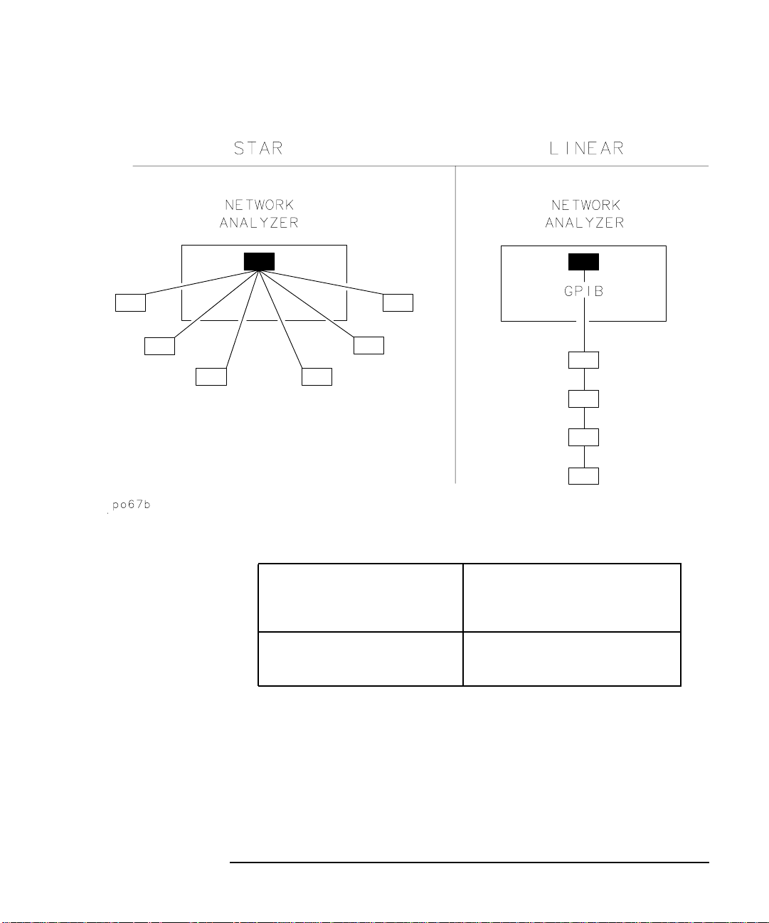
Figure 1-5 GPIB Connection Conﬁgurations

Installing the Analyzer

Step 4. Conﬁgure the Analyzer

Table 1-1 Maximum GPIB Cable Lengths

Instruments/Peripherals in System

Two

Fifteen (max)

ET User’s Guide 1-13

Maximum GPIB Cable Length between Each Pair of Devices

4 m

20 m (total)

Installing the Analyzer

Select Copy Port

Select

Print/Plot GPIB Addr

Enter

Select Copy Port

Select

Print/Plot GPIB Addr

Enter

Step 4. Conﬁgure the Analyzer

Parallel and Serial Connections

Other Connections If you plan to use a keyboard, barcode reader, external video monitor, or

To Set GPIB Addresses

Parallel and serial devices often require speciﬁc cables—check their manuals for details. Parallel cable length should not exceed 25 feet. The analyzer may experience problems talking to a printer if this length is exceeded. Connect the required control cables and secure them. (Tighten the knurled screws or comparable fasteners.)

external detectors, connect them to the appropriate rear panel connectors. See Figure 1-4, “Analyzer Rear Panel Line Module and

Selected Connectors.” Also see Chapter 7, “Front/Rear Panel,” for more

information on front and rear panel connectors. To communicate via GPIB, each external device must have a unique

address and the network analyzer must recognize each address. T o check or set each external device's actual address, refer to the device's manual (most addresses are set with switches).

The following are examples of how to check or set the device's recognized address on the network analyzer:

Printer: Press . Use the

front panel knob to highlight the line that reads HP Printer PCL GPIB. Press . The second line of the screen displays settings: in this case the address. The default address is 5, however most printers are factory set to address 1 (one). To change the recognized address, press

HARDCOPY

number

NOTE Only one hardcopy GPIB address can be set at a time. Changing the

Plotter: Press . Use the

front panel knob to highlight the line that reads HP Plotter HPGL GPIB. Press . The second line of the screen displays settings: in this case the address. The default address is 5 and most plotters are factory set to address 5, so changing the address is probably not necessary. To change the recognized address, press

printer address, for example, changes the plotter to the same address.

1-14 ET User’s Guide

HARDCOPY

number

Installing the Analyzer

GPIB

8712ET Address

8714ET Address

Enter

Select Copy Port

Select

Select Copy Port

Select

Select Copy Port

Select

LAN Printr IP Addr

Select Copy Port

Step 4. Conﬁgure the Analyzer

To Conﬁgure Peripheral Settings

Analyzer: Press ,

network analyzer's address will appear (the default is

16). To change the address, press , .

If your system uses serial or parallel peripherals, follow the guidelines below to conﬁgure the system. Refer to the peripheral's manual for correct cables and settings. The parallel and serial ports have standard Centronics DB-25 and RS232 pinouts respectively as explained in

Chapter 7, “Front/Rear Panel.”

Serial Devices: Press . Use the

entry controls to highlight your type of printer or plotter, and press . If the baud rate or handshake at the top of the screen are incorrect, use the softkeys to change them.

Parallel Devices: Press . Use the

entry controls to highlight your type of printer or plotter, and press .

LAN Printer: Press . Use the

entry controls to highlight HP LaserJet PCL5/6 PCL5 LAN, and press . If the printer IP

address at the top of the screen is incorrect, press

SYSTEM OPTIONS

or . The

number

HARDCOPY

to enter the correct IP address.

NOTE When is selected, the ﬁrst two lines in the box at

NOTE Use a PCL5 printer for fastest hardcopies. See “Conﬁgure the Hardcopy

the top of the display screen show the current settings.

Port” on page 4-72 for more information.

ET User’s Guide 1-15

Installing the Analyzer

Step 4. Conﬁgure the Analyzer

Installing the Analyzer in a Rack

Use only the recommended rack mount kit (Option 1CM when ordered with the analyzer or part number 08712-60036 when ordered separately) with this instrument; it needs side support rails. Do not attempt to mount it by the front panel (handles) only. This rack mount kit allows you to mount the analyzer with or without handles.

To install the network analyzer in an HP/Agilent 85043D rack, follow the instructions in the rack manual.

CAUTION To install the network analyzer in other racks, note that they may

promote shock hazards, overheating, dust contamination, and inferior system performance. Consult your Agilent customer engineer about installation, warranty, and support details.

CAUTION VENTILATION REQUIREMENTS: When installing the product in a

cabinet, the convection into and out of the instrument must not be restricted. The ambient temperature (outside the cabinet) must be less than the maximum operating temperature of the instrument by 4 °C for every 100 watts dissipated in the cabinet. If the total power dissipated in the cabinet is greater than 800 watts, then forced convection must be used.

Place other system instruments (computer, printer, plotter) where convenient, within the GPIB cable length limits (see Table 1-1,

“Maximum GPIB Cable Lengths,” on page 1-13) or other interface

cabling limits.

1-16 ET User’s Guide

Installing the Analyzer

Preventive Maintenance

Preventive maintenance consists of two tasks. It should be performed at least every six months—more often if the instrument is used daily on a production line or in a harsh environment.

Clean the Display Use a soft cloth and, if necessary, a mild cleaning solution to clean the

display.

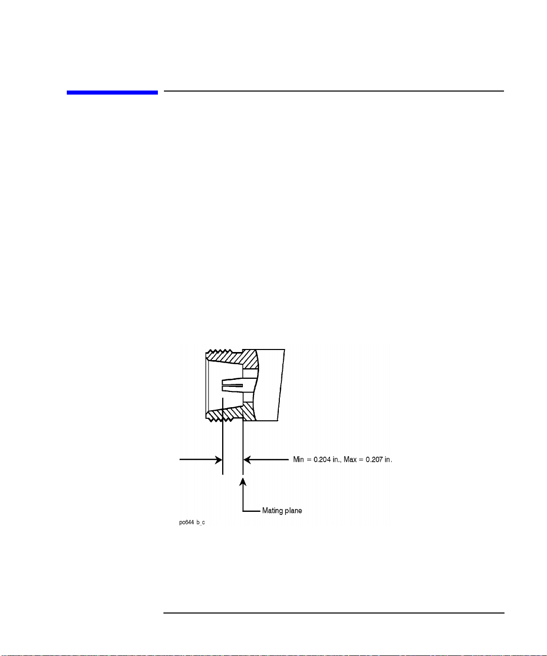
Check the RF Front Panel Connectors

Figure 1-6 Maximum and Minimum Protrusion of Center Conductor from

Visually inspect the front panel connectors. The most important connectors are those to which the DUT is connected, typically the RF cable end or the RF IN connector. All connectors should be clean and the center pins centered. The ﬁngers of female connectors should be unbroken and uniform in appearance. If you are unsure whether the connectors are good, gauge the RF IN and RF OUT connectors to conﬁrm that their dimensions are correct.

Mating Plane

ET User’s Guide 1-17

2 Getting Started

ET User’s Guide 2-1

Getting Started

Introduction

The 8712ET and 8714ET are easy-to-use, fully integrated RF component test systems.Each instrument includes a synthesized source, a wide dynamic range receiver, and a built-in test set. Controls are grouped by functional block, and settings are displayed on the instrument screen. This section familiarizes new users with the layout of the front panel and the process of entering measurement parameters into the analyzer.

Figure 2-1 Network Analyzer Front Panel Features

2-2 ET User’s Guide

Getting Started

Softkeys

Sweep Time

Front Panel Tour

1 The CRT Display The analyzer's large CRT displays data, markers, limit lines, Instrument BASIC

(IBASIC) programming code, softkey menus, and measurement parameters quickly and clearly. Refer to “Display” on page 7-16 for more information.

2 The key simpliﬁes measurement setups. The key allows quick

BEGIN BEGIN BEGIN

and easy selection of basic measurement parameters for a user-selected class of devices (e.g., ﬁlters, ampliﬁers, or mixers). For example, when making a transmission measurement, selecting Filter as your device type puts the analyzer into narrowband detection mode, maximizing measurement dynamic range. In comparison, selecting Mixer as your device type puts the analyzer into broadband detection mode, enabling frequency-translation measurements. This capability allows new users to start making measurements with as few as four keystrokes.

3 MEAS The measure keys select the measurements for each measurement channel. The

analyzer's measurement capabilities include transmission, reﬂection, power, conversion loss, and multiport selection (for use with multiport test sets).

4 SOURCE The source keys select the desired source output signal to the device under test, for

example, selecting source frequency range or output power. The source keys also control sweep time, number of points, and sweep triggering.

5 CONFIGURE The conﬁgure keys control receiver and display parameters. These parameters include

receiver bandwidth and averaging, display scaling and format, marker functions, and instrument calibration.

6 SYSTEM The system keys control system level functions. These include instrument preset,

save/recall, and hardcopy output. GPIB parameters and IBASIC are also controlled with these system keys.

7 The Numeric Keypad Use the number keys to enter a speciﬁc numeric value for a chosen parameter. Use the

key or the softkeys to terminate the numeric entry with the appropriate

HARDKEYS

ENTER

units. You can also use the front panel knob for making continuous adjustments to parameter values, while the keys allow you to change values in steps. Hardkeys are front panel keys physically located on the instrument front panel. In text,

these keys will be represented by the key name with a box around it such as:

PRESET

Softkeys are keys whose labels are determined by the analyzer's ﬁrmware. The labels are on the screen next to the 8 blank keys, which are located along the right edge of the analyzer’s display. In text, these softkeys will be represented by the key name with

shading behind it such as: .

ET User’s Guide 2-3

Getting Started

42.5

Entering Measurement Parameters

This section describes how to input measurement parameter information into the network analyzer.

NOTE When entering parameters, you can use the numeric key pad, as

described in each example, or you can use the keys or the front panel knob to enter data.

NOTE When you are instructed to enter numeric values in this manual, it often

can get cluttered and confusing to depict each key stroke. So in this manual, numbers (no matter how many characters) are depicted inside one keycap. F or example, if you are instructed to enter the number−42.5, it will be depicted inside one keycap like this: . To enter this number , the following keys need to be pressed in succession:

You can follow along with these examples by connecting the ﬁlter and cable that were supplied with your instrument as shown in Figure 2-2.

−

− 4 2

Figure 2-2 Connect the Filter to the Analyzer

2-4 ET User’s Guide

Getting Started

User Preset

Factory Preset

User Preset

Factory Preset

Entering Measurement Parameters

Presetting the Analyzer

Press the key and then press either or

PRESET

. The key returns the analyzer to user-deﬁned preset settings you may have saved as ﬁle UPRESET.STA. If this ﬁle doesn’t exist, you can create it by following the instructions in the pop-up message that appears when the key is pressed. When the

key is pressed, the following major default conditions apply:

Frequency range (8712ET) 0.3 to 1300 MHz Frequency range (8714ET) 0.3 to 3000 MHz Power level Measurement Channel 1

0 dBm Transmission

measurement Measurement Channel 2

Off

measurement Format Log Magnitude Number of points 201 Sweep time Auto

NOTE The measurement parameters that you enter will be retained in the

NOTE Refer to Chapter 11, “Factory Preset State and Memory Allocation, ” for a

Scale 10 dB/div Reference 0 dB System Bandwidth Medium wide

1. Preset power level can be set to other than 0 dBm if desired. See “Entering Source Power Level” on page 2-6 for more information.

analyzer's memory when the power is turned off, and will be restored when the power is turned back on.

comprehensive table of factory preset conditions.

ET User’s Guide 2-5

Getting Started

Start

MHz

Stop

MHz

Center

Span

Disp Freq Resolution

Level

dBm

Level

1.6

dBm

Pwr Level at Preset

2.5

dBm

Autoscale

Scale/Div

Enter

Reference Position

Enter

Reference Level

Enter

Entering Measurement Parameters

Entering Frequency Range

1. Press the key to access the frequency softkey menu.

FREQ

2. To change the low end of the frequency range to 10 MHz, press

3. To change the high end of the frequency range to 900 MHz, press

900

4. You can also set the frequency range by using the and softkeys. For instance, if you set the center frequency to

160 MHz and the span to 300 MHz, the resulting frequency range would be 10 to 310 MHz.

NOTE When entering frequencies, be sure to terminate your numeric entry

with the appropriate softkey to obtain the correct units. If you use the

ENTER

key to terminate a frequency entry, the units default to Hz.

The default displayed frequency resolution is kHz. You can change the resolution by pressing , and then

FREQ

selecting a new resolution.

Entering Source Power Level

1. Press the key to access the power level softkey menu.

2. To change the power level to 3 dBm, press and or

ENTER

3. To change the power level to−1.6 dBm, press

or .

ENTER

POWER

−

Scaling the Measurement Trace

4. To change the power level that will always be restored when you

preset the analyzer, press and or . This entry does not affect the current power level.

ENTER

1. Press the key to access the scale menu.

SCALE

2. To view the complete measurement trace on the display, press

3. To change the scale per division to 5 dB/division, press

4. To move the reference position (indicated by the symbol on the left

side of the display) to the ﬁrst division down from the top of the display, press . Figure 2-3 shows

how each reference position is identiﬁed.

5. To change the reference level to 0 dB, press

2-6 ET User’s Guide

Figure 2-3 Reference Positions

User Preset

Factory Preset

Transmissn

Reﬂection

Getting Started

Entering Measurement Parameters

Entering Active Measurement Channel and Measurement Type

The and keys allow you to choose which

MEAS 1 MEAS 2

measurement channels are active, and measurement parameters for the channels. When a particular measurement channel is selected, its display is brighter than the other channel, and any changes made to measurement parameters will affect only the selected measurement channel. (Some measurement parameters cannot be independently set on each measurement channel. F or these parameters , both c hannels will be affected regardless of selected channel status.)

1. To measure transmission on measurement channel 1 and reﬂection on measurement channel 2, press the following keys:

PRESET

MEAS 2

2. Both channels' measurements are now visible on the analyzer's display screen. Note that the selected measurement channel's (channel 2) measurement trace is brighter than the other measurement channel's trace. Refer to Figure 2-4.

MEAS 1

ET User’s Guide 2-7

Getting Started

Meas OFF

More Display

Split Disp FULL split

Entering Measurement Parameters

Figure 2-4 Both Measurement Channels Active

Viewing Measurement Channels

3. To view only the measurement channel 2 reﬂection measurement, press .

4. To view both measurement channels again, press .

5. To view both measurement channels separately on a split screen, press . Refer to

Figure 2-5, “Split Display.”

2-8 ET User’s Guide

MEAS 1

DISPLAY

Figure 2-5 Split Display

Getting Started

Entering Measurement Parameters

You have now learned how to enter common measurement parameters and how to manipulate the display for optimum viewing of your measurement. You can now proceed on to performing the operator's check, or refer to Chapter 3, “Making Measurements,” for detailed information on making speciﬁc types of measurements.

ET User’s Guide 2-9

Getting Started

Performing the Operator's Check

The operator's check should be performed when you receive your instrument, and any time you wish to have conﬁdence that the analyzer is working properly. The operator's check does not verify performance to speciﬁcations, but should give you a high degree of conﬁdence that the instrument is performing properly if it passes.

The operator's check consists of making the following measurements with the cable that was supplied with your analyzer:

• transmission

• broadband power

• reﬂection

• reﬂection (with a 50 Ω or 75 Ω load, instead of the cable)

Equipment List

To perform the operator's check, you will need the following:

• A known good cable such as the one that was supplied with your analyzer. The cable you use should have ≤0.5 dB of insertion loss up to 1.3 GHz and ≤0.75 dB of insertion loss from 1.3 to 3.0 GHz.

• A known good load (> 40 dB return loss) that matches the test port impedance of your analyzer such as one from calibration kit 85032B/E (50 Ω) or 85036B/E (75 Ω).

2-10 ET User’s Guide

Getting Started

User Preset

Factory Preset

Enter

dBm

Default Response

Performing the Operator's Check

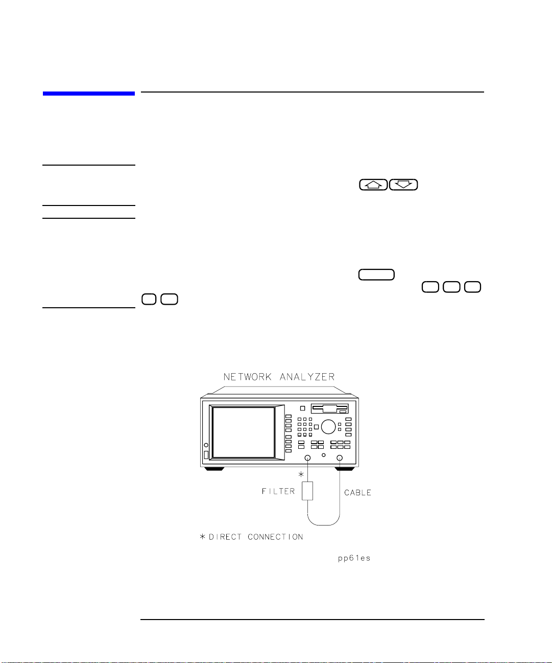
Make a Transmission Measurement

1. Connect the equipment as shown in Figure 2-6. Use a known good cable such as the one that was supplied with your analyzer.

NOTE The quality of the cable will affect these measurements; make sure you

use a cable with the characteristics described in “Equipment List” on

page 2-10.

Figure 2-6 Equipment Setup for Performing the Operator’s Check

2. Press or

3. Press .

4. Press .

5. Verify that the data trace falls within ±0.5 dB of 0 dB. See Figure 2-7 for a typical 8714ET result. The 8712ET should look similar, but end at 1300 MHz.

ET User’s Guide 2-11

PRESET

POWER 0 CAL

SCALE .1

Getting Started

Performing the Operator's Check

Figure 2-7 Verify Transmission Measurement

2-12 ET User’s Guide

Getting Started

Power

Start

MHz

Enter

dBm

Performing the Operator's Check

Make a Broadband Power Measurement

1. Leave the cable connected to the analyzer as shown in Figure 2-6.

NOTE The quality of the cable will affect these measurements; make sure you

use a cable with the characteristics described in “Equipment List” on

page 2-10.

2. Press

3. Press (unless done in the previous measurement).

4. V erify that the data trace is within±2 dB of 0 dBm. See Figure 2-8 for a typical 8714ET result. The 8712ET should look similar, but end at 1300 MHz.

Figure 2-8 Verify Broadband Power Measurement

MEAS 1

POWER 0

FREQ

SCALE

ET User’s Guide 2-13

Getting Started

User Preset

Factory Preset

Reﬂection

Enter

dBm

Default 1-Port

Performing the Operator's Check

Make a Reﬂection Measurement

1. Leave the cable connected to the analyzer as shown in Figure 2-6.

NOTE The quality of the cable will affect these measurements; make sure you

use a cable with the characteristics described in “Equipment List” on

page 2-10.

Press or

PRESET

SCALE 10

MEAS 1

3. Press .

4. Press .

5. Verify that the data trace falls completely below −16 dB. See Figure

2-9 for a typical 8714ET result. The 8712ET should look similar, but

end at 1300 MHz.

POWER 0 CAL

2-14 ET User’s Guide

Figure 2-9 Verify Reﬂection Measurement

Getting Started

Performing the Operator's Check

6. Disconnect the cable and connect a known good load to the RF OUT port as shown in Figure 2-10.

ET User’s Guide 2-15

Getting Started

Reference Level

Trigger

Hold

Performing the Operator's Check

Figure 2-10 Connect the Load

7. Verify that the data trace falls below −30 dB. If the data trace is off the screen, press and the key until the trace moves up onto the screen.

SCALE

This concludes the operator's check. However, further conﬁdence can be obtained by performing the following:

• Measure a known ﬁlter to verify that its measured response is the same as is expected. (A 175 MHz ﬁlter is supplied with the analyzer.) Verify both the frequency accuracy and noise ﬂoor.

• Check broadband response with the ﬁlter using conversion-loss mode (same as B*/R*).

• If the analyzer's frequency accuracy is critical for your application, verify a CW frequency using a frequency counter. Verify to ±.005% accuracy (for example, ± 2500 Hz at 500 MHz). Ensure that the analyzer is placed in trigger-hold mode (press

) to measure frequencies.

2-16 ET User’s Guide

Getting Started

Performing the Operator's Check

If the Analyzer Fails the Operator's Check

First, repeat the operator's check using a different cable and load to eliminate these as a possible cause of failure. If your analyzer does not meet the criteria in the operator's check, your analyzer may need adjustment or servicing. Contact any Agilent Technologies sales or service ofﬁce for assistance. Refer to Table 9-8, “Agilent Technologies

Sales and Service Ofﬁces,” on page 9-48 for the nearest ofﬁce. Before

shipping your analyzer, ﬁll out and attach the blue repair tag, located at the back of the analyzer’s Service Guide.

ET User’s Guide 2-17

3 Making Measurements

ET User’s Guide 3-1

Making Measurements

Introduction

This chapter provides an overview of basic network analyzer measurement theory, a section explaining the typical measurement sequence, a segment describing the use of the key, and detailed examples of the following measurements:

• “Measuring Transmission Response” on page 3-16

• “Measuring Reﬂection Response” on page 3-33

• “Making a Power Measurement using Broadband Detection” on

page 3-40

• “Measuring Conversion Loss” on page 3-46

• “Making Measurements with the Auxiliary Input” on page 3-52

• “Measuring Group Delay” on page 3-54

• “Measuring Impedance using the Smith Chart” on page 3-58

• “Measuring Impedance Magnitude” on page 3-64

BEGIN

3-2 ET User’s Guide

Measuring Devices with Your Network Analyzer

This section provides a basic overview of how the network analyzer measures devices. The analyzer has an RF signal source that produces an incident signal that is used as a stimulus to the device under test. Your device responds by reﬂecting a portion of the incident signal and transmitting the remaining signal. If the device is passive, some of the transmitted signal will be absorbed, indicating a “lossy” device. If the device is active, the transmitted signal may be ampliﬁed, indicating that the device has gain. Figure 3-1 shows how a device under test (DUT) responds to an RF source stimulus.

Figure 3-1 DUT Response to an RF Signal

Making Measurements

Measuring Devices with Your Network Analyzer

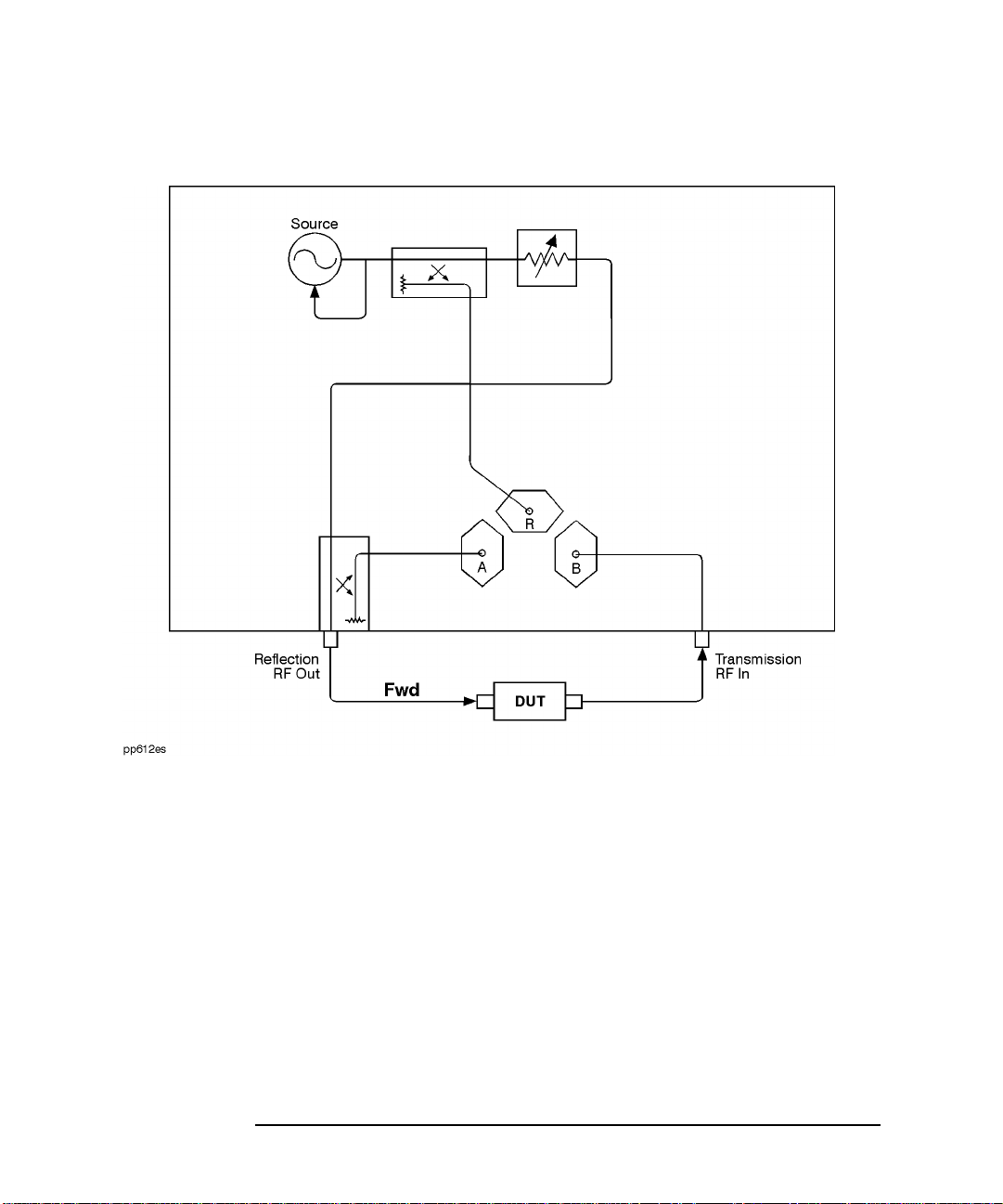
Refer to Figure 3-2 for the following discussion regarding detection schemes and modes. The transmitted signal (routed to input B) and the reﬂected signal (input A) are measured by comparison to the incident signal. The analyzer couples off a small portion of the incident signal to use as a reference signal (routed to input R). Sweeping the source frequencies, the analyzer measures and displays the response of your test device. Figure 3-2 shows the transmitted, reﬂected, and reference signal inputs.

ET User’s Guide 3-3

Making Measurements

Measuring Devices with Your Network Analyzer

Figure 3-2 Simpliﬁed Block Diagram

3-4 ET User’s Guide

This page intentionally left blank.

Making Measurements

Measuring Devices with Your Network Analyzer

ET User’s Guide 3-5

Making Measurements

Measuring Devices with Your Network Analyzer

Refer to Figure 3-3 for the following discussion. The network analyzer receiver has two signal detection modes:

• broadband detection mode

• narrowband detection mode

There are two internal broadband detectors: B* and R*. External broadband detectors can also be used when connected to the X and Y ports on the rear panel of the analyzer. When the network analyzer is in the broadband detection mode, it measures the total power of all signals present at these measurement ports, independent of signal frequency. This enables the characterization of frequency translation devices such as mixers, receivers, and tuners, where the RF input and output frequencies are not the same. Figure 3-3 labels the transmitted signal for broadband detection input as B*, and the reference signal as R*.

When the network analyzer is in the narrowband detection mode, the receiver is tuned to the source frequency. This technique provides greater dynamic range by decreasing the receiver's bandwidth. Figure 3-3 shows receiver B as the narrowband detection input for the transmitted signal, and receiver R as the narrowband detection input for the reference signal.

3-6 ET User’s Guide

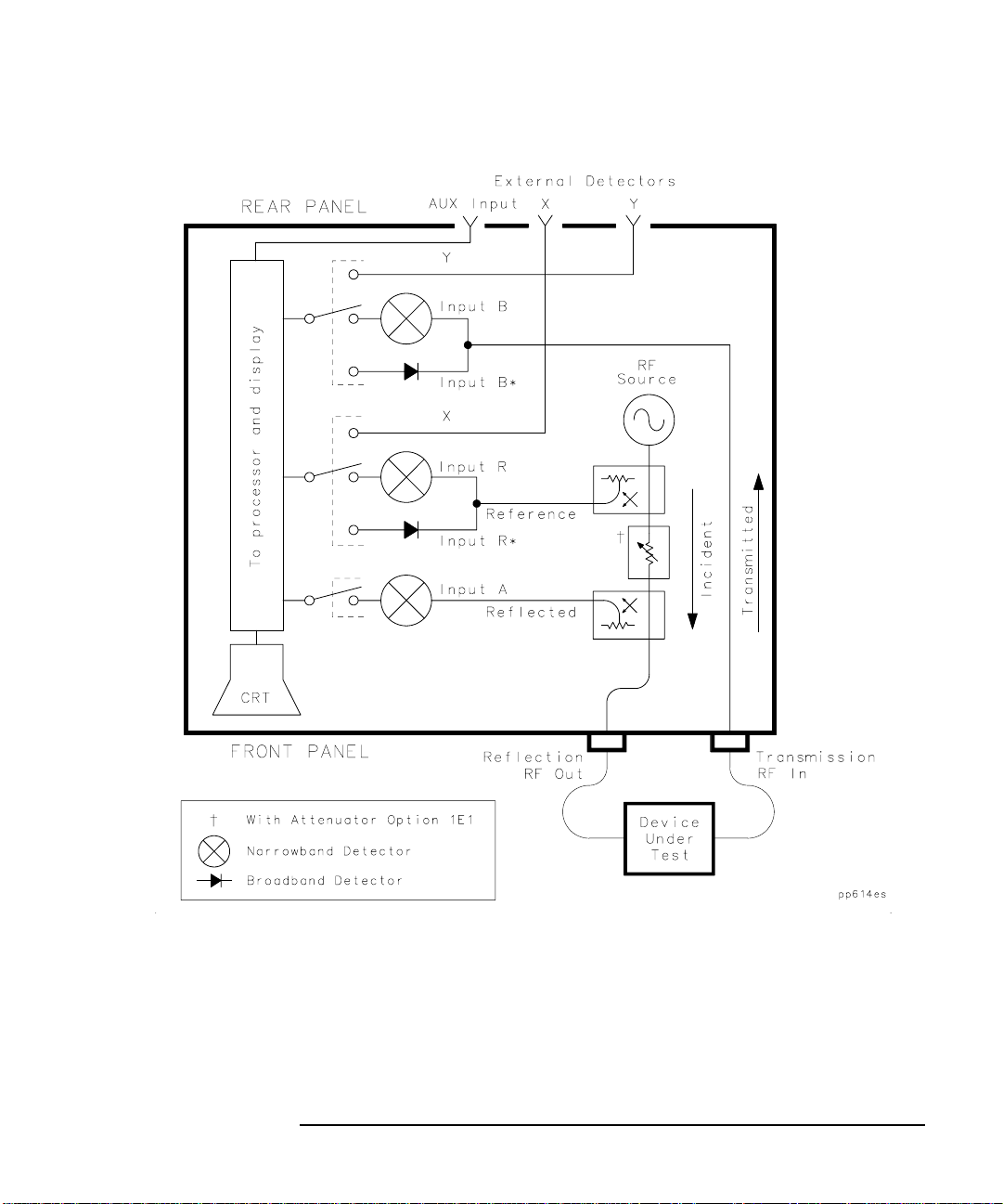
Figure 3-3 Block Diagram

Making Measurements

Measuring Devices with Your Network Analyzer

ET User’s Guide 3-7

Making Measurements

Measuring Devices with Your Network Analyzer

The following table shows the correlation between different types of measurements, input channels, and signals.

Measurement Detection Mode Input Channels Input Signals

Transmission Reﬂection Power Conversion Loss

Narrowband Narrowband Broadband Broadband

B/R A/R

B*/R*

transmitted/incident reﬂected/incident transmitted transmitted/incident

Attenuation and Ampliﬁcation in a Measurement Setup

The measurement setup that you use may require attenuation or ampliﬁcation. The following sections describe when to use them.

When to Use Attenuation

• For accurate measurements, use external attenuation to limit the power at the RF IN port to +10 dBm (for narrowband-detection measurements) or +16 dBm (for broadband measurements).

CAUTION Always use attenuation on the TRANSMISSION RF IN port if your test

device's output power exceeds the receiver damage limit of +20 dBm or ±30 Vdc.

• Use attenuation on the RF IN port to reduce mismatch errors. See

“Reducing Mismatch Errors” on page 5-15 for more information.

3-8 ET User’s Guide

Making Measurements

More Cal

System Z0

50Ω 75

Measuring Devices with Your Network Analyzer

When to Use Ampliﬁcation

• For accurate measurements, ampliﬁcation may be needed on the analyzer's RF OUT port. Use ampliﬁcation when your test device requires input power that exceeds the analyzer's maximum speciﬁed output power.

NOTE If you use an ampliﬁer between the analyzer’s output port and your DUT,

you won’t be able to measure the reﬂection response of your DUT.

The maximum speciﬁed output power is dependent upon the option conﬁguration of your analyzer as well as the frequency range of your test setup. It ranges from +6 to +16 dBm. See Chapter 9,

“Speciﬁcations,” to determine the maximum speciﬁed output power of

your analyzer.

When to Change the System Impedance

Your analyzer has a system characteristic impedance of either 50 or 75 ohms, yet may be changed to the alternate impedance. If using minimum-loss pads for impedance conversions, the alternate impedance should be selected so that the measurement results are displayed relative to the conversion impedance.

For example, if you have a 50 ohm instrument and are making 75 ohm measurements, you may be using 50 to 75 ohm minimum-loss pads. Measurement results can be reported relative to 75 ohms, not 50 ohms, if the alternate system impedance is selected. This includes marker readouts, Smith chart results, or SRL impedance computations (Option 100).

To change the system impedance, press the following keys on the analyzer:

CAL

οr

The built-in cal kit selections will be converted to the selected system impedance.

ET User’s Guide 3-9

Ω

Making Measurements

Measuring Devices with Your Network Analyzer

The Typical Measurement Sequence

A typical measurement consists of performing four major steps:

Step 1. Enter the Measurement Parameters

Step 2. Calibrate the Analyzer

Step 3. Connect the Equipment

Step 4. View and Interpret the Measurement

The easiest way to set up the analyzer's parameters for a simple measurement is to use the key. When this key is selected, the analyzer automatically sets up a generic set of parameters to match the device type you choose. (See “Using the BEGIN Key to Make

Measurements” on page 3-11.)

For measurements that require you to enter your own speciﬁc measurement parameters (such as frequency range, source power level, number of points, and sweeptime), use the instrument’s keys to enter your selections rather than using the key. See the measurement examples, located later in this chapter.

Your analyzer can provide highly accurate measurements without performing any additional user-deﬁned calibrations if certain conditions are met. Chapter 6, “Calibrating for Increased Measurement Accuracy,” explains when additional user-deﬁned calibration is necessary.

Connect the DUT and any other required test equipment. See the measurement examples later in this chapter for typical equipment setup conﬁgurations.

Use the , , and functions to optimize viewing of the measurement results.

Markers, limit lines, and hard copies of the display are common means of interpreting measurement results.

SCALE DISPLAY FORMAT

BEGIN

See Chapter 4, “Using Instrument Functions,” for detailed information on using instrument functions to view and interpret your measurements.

3-10 ET User’s Guide

Using the BEGIN Key to Make Measurements

Figure 3-4 The BEGIN Key

Making Measurements

Using the BEGIN Key to Make Measurements

The key allows you to quickly and easily conﬁgure the analyzer

BEGIN

(from the condition) to measure the following:

• ampliﬁers

• ﬁlters

• broadband passive devices (a cable, for example)

• mixers

• cable fault location and structural return loss (Option 100 only)

Conﬁguring basic measurements from the key helps you ensure correct instrument setup. The analyzer guides you through the initial steps and conﬁgures itself for the device type you select.

ET User’s Guide 3-11

PRESET

BEGIN

Making Measurements

Using the BEGIN Key to Make Measurements

BEGIN Key Overview

The key sets up a generic instrument state for the testing of

BEGIN

various types of devices. The key has two different behaviors, depending on whether

BEGIN

you are selecting a new device type, or a new measurement type.

Selecting a New Device

Selecting a New Measurement

When you use the key to select a new device type and measurement, the analyzer does the following:

• presets the analyzer (except for external reference parameters, and trigger mode)

• takes a sweep

• autoscales the measurement

• places a marker on the maximum or minimum point (depending on the type of measurement)

• makes the marker active

• modiﬁes the sweep time (Option 100 only)

See Table 3-1, “Measurement Conﬁgurations from the BEGIN Key,” on

page 3-14 for a table of parameters for each measurement type.

Once you have selected your device, you can use the softkeys to select the measurement you wish to make. When you select a new measurement, a preset is not done. It is assumed that you are simply changing measurement types and that you may have already changed some of the analyzer's parameters (such as frequency, power, etc.) for your DUT. In this situation, you would probably not want these parameters changed for subsequent measurements.

BEGIN

NOTE If the new measurement selected is a broadband measurement such as

power, or conversion loss, the start frequency is limited to at least 10 MHz. Therefore, if your customized setup contains a start frequency below 10 MHz and you choose power, or conversion loss, the start frequency will be changed to 10 MHz. The stop frequency will remain unchanged, unless it was set to below 10 MHz.

3-12 ET User’s Guide

Making Measurements

User Preset

Factory Preset

Transmissn

Reﬂection

Power

Ampliﬁer

Conversion Loss

Mixer

Using the BEGIN Key to Make Measurements

The BEGIN Key and Measurement Channels

The key is designed to work when measurement channel 1 is

BEGIN

active. However, it does change the mode of measurement channel 2 as well.

If measurement channel 2 is active when the key is used to select a new device type, measurement channel 2 is turned off, and measurement channel 1 is made active.

If measurement channel 2 is active when the key is used to select a new measurement type, measurement channel 2 will be left on and active. However, the analyzer then proceeds to set up channel 1 for the requested measurement type, even though channel 2 is the active channel.

BEGIN

Using the BEGIN Key to Conﬁgure Measurements

This procedure shows you how to conﬁgure the network analyzer for measurements.

1. Press ( or ). Presetting the instruments puts it into a known state with predeﬁned parameters.

2. Press and then use a softkey to select the type of device that you will be measuring (ampliﬁer, ﬁlter, broadband passive device, mixer, or cable—Option 100 only).

PRESET

BEGIN

3. Connect your test device to the network analyzer.

4. Use the softkeys to select the type of measurement you want to make:

• Press if you want to measure the transmission

characteristics of an ampliﬁer, ﬁlter, or broadband passive device.

• Press if you want to measure the reﬂection

characteristics of your device.

• Press if you want to measure the RF power of a device.

(The selection is under the menu.)

• Press if you want to measure the conversion

loss of a device. (The selection is under the

menu.)

ET User’s Guide 3-13

Making Measurements

SRL

Cable

Fault Location

Cable

SRL

Fault Location

Using the BEGIN Key to Make Measurements

• Press (Option 100 only) if you want to measure the structural return loss of a cable. (The selection is under the

menu.)

• Press (Option 100 only) if you want to measure the cable fault location. (The selection is under the menu.)

Depending on your selection, the analyzer is set to one of the following conﬁgurations. (The and conﬁgurations are discussed in the Option 100 User's Guide Supplement.)

Table 3-1 Measurement Conﬁgurations from the BEGIN Key

Transmission Reﬂection Power Conversion Loss

Frequency Range (8712ET)

Frequency Range (8714ET)

Measurement Channel 1

Detection Mode Narrowband Narrowband Broadband Internal Broadband Internal Measurement

Paths

0.300 MHz to 1300 MHz

0.300 MHz to 3000 MHz

Transmission Reﬂection Power Conversion Loss

B/R A/R B* B*/R*

0.300 MHz to 1300 MHz

0.300 MHz to 3000 MHz

10 MHz to 1300 MHz

10 MHz to 3000 MHz

10 MHz to 1300 MHz

10 MHz to 3000 MHz

The following measurement conﬁgurations apply to all of the measurement types in the previous table:

Power Level Factory preset or user preset power

level

Measurement Channel 2 Off Format Log Mag Number of Points 201 Sweep Time Mode Auto Sweep Triggering Continuous Averaging Off System Bandwidth Medium Wide

1. Factory preset power level is user-deﬁned by using the “Pwr Level at Preset” softkey. The factory default is 0 dBm.

3-14 ET User’s Guide

Making Measurements

Autost

User BEGIN

Recall Program

User BEGIN on OFF

User BEGIN

Using the BEGIN Key to Make Measurements

AUTOST Files

When the analyzer's power is turned on, it ﬁrst checks for an IBASIC autostart ﬁle (AUTOSTART.BAS) on the non-volatile RAM disk and then on the 3.5” disk. If found, the ﬁle is loaded and run. This feature simpliﬁes the task of turning on an automated test station at the beginning of a working day or test session. To manually load and run an autostart ﬁle, press .

BEGIN

The User BEGIN Function

The softkey gives you the capability to redeﬁne the

BEGIN

key to deﬁne macros such as:

• softkeys to implement fast save/recall

• softkeys to implement most-used functions or features

• softkeys to implement often-used features that involve a number of

Macros must be deﬁned with an IBASIC program. If no program is currently installed (either by AUTOST or

program.

key menu and install user-deﬁned macro functions. Use this

steps

), the analyzer will automatically create a default

selects the key menu to "user" mode

when on, and to normal operation when off. Once you have changed the mode to on, the same menu

will be displayed for subsequent key presses of the hardkey. (This is not true if your IBASIC program has changed. If the program has changed, the mode is reset to off.)

Use of the function does not restrict access to any normally available instrument feature (such as marker functions), nor does this key affect sweep update rates.

Refer to the IBASIC example programs provided on the Example Programs Disk for implementation requirements. Keystroke recording may be used to modify or update programs.

See the Automating Measurements User’s Guide Supplement for more information.

ET User’s Guide 3-15

BEGIN

Making Measurements

User Preset

Factory Preset

Measuring Transmission Response

This section uses an example measurement to describe how to calibrate for and make a basic transmission response measurement. This example uses an enhanced response calibration. See the table below for a list of all possible calibration choices for a transmission response measurement.

TIP An optimum calibration is critical for achieving best measurement

accuracy. Refer to Chapter 6, “Calibrating for Increased Measurement

Accuracy,” for detailed information about all of the various aspects of

calibration.

Table 3-2 Calibration Choices for a Transmission Response Measurement

Measurement Type Calibration Choices

Transmission Default Response

Response Response & Isolation Enhanced Response Normalize

NOTE This example measurement uses the default instrument parameters for

In this example, a bandpass ﬁlter like the one that was supplied with your network analyzer is used.

Enter the Measurement Parameters

Press ( or ) on the analyzer to set the analyzer to the default mode which includes measuring transmission on measurement channel 1.

a transmission measurement. If your particular transmission measurement requires speciﬁc parameters (such as frequency range, source power level, number of data points, and sweeptime), enter them now.

3-16 ET User’s Guide

PRESET

Making Measurements

Measuring Transmission Response

Perform an Enhanced Response Calibration

An enhanced response calibration uses known standards to correct for source match and frequency response errors when using narrowband detection. When you perform an enhanced transmission response calibration, the analyzer performs correction at each data point across the selected frequency band. The default number of data points per sweep is 201, but you can select any number between 3 and 1601. Interpolation recalculates the error correction array for reduced frequency spans. If the frequency span is increased, the calibration is invalidated, and the default response calibration is automatically restored.

To perform an enhanced transmission response calibration, you will need one of the following calibration kits depending on the nominal impedance of your analyzer:

Cal Kit Model

Number

85039B 75 Ω type-F ✓✓ 85036B 75 Ω type-N ✓✓ 85036E 75 Ω type-N ✓ 85032B 50 Ω type-N ✓✓ 85032E 50 Ω type-N ✓ 85031B 50 Ω APC-7 N/A N/A 85033D 50 Ω 3.5 mm ✓✓ 85038A 50 Ω 7-16 ✓✓ 85038F 50 Ω 7-16 ✓

85038M 50 Ω 7-16 ✓

Impedance

Connector

Type

For Use with Male Test Ports

For Use

with Female

Test Ports

ET User’s Guide 3-17

Making Measurements

More Cal

Cal Kit

Enhanced Response

Measuring Transmission Response

NOTE By convention, cal kit labels in the analyzer indicate the sex of the port

with which they are used. For example, the default cal kit for the analyzer is type-N female because the front panel RF ports are female (the calibration standards, in turn, have male connectors).

Calibrating for Insertable Devices

When measuring a through-standard during calibration, the test ports normally mate directly together. For example, two cables with the appropriate connectors can be connected directly without a through-adapter, resulting in a zero-length through-standard. An insertable device is a device that can be inserted in place of a zero-length through-standard. It has the same type of connector on each port, but with a different sex, or the same type of sexless connector on each port (APC-7, for example).

Chapter 6 provides detail about when this calibration is necessary, and

information about other calibrations available for transmission measurements. If you wish to perform an enhanced response calibration on your insertable device, perform the following steps:

NOTE If you are going to be using calibration standards other than the default

(female type-N), you must select the connector type by pressing

and then selecting the appropriate type.

1. Press .

2. The instrument prompts you to connect four standards—open, short, load, and through cable—as shown in the following graphic.

3-18 ET User’s Guide

CAL

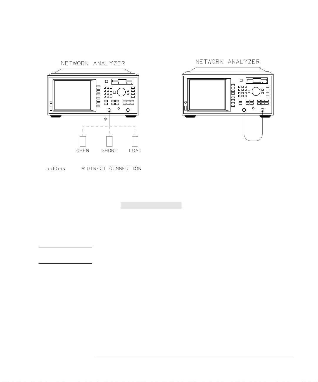
Making Measurements

Measure Standard

Measuring Transmission Response

Open, Short, Load Connections Through-Cable Connection

3. Press after connecting each standard.

4. The analyzer will measure each standard and then calculate the new calibration coefﬁcients. The message "Calibration complete." will appear for a few seconds when the analyzer is done calculating the new error correction array.

NOTE Changing sweep frequencies (and other source parameters) may affect

your calibration. See Chapter 6 for more information.

ET User’s Guide 3-19

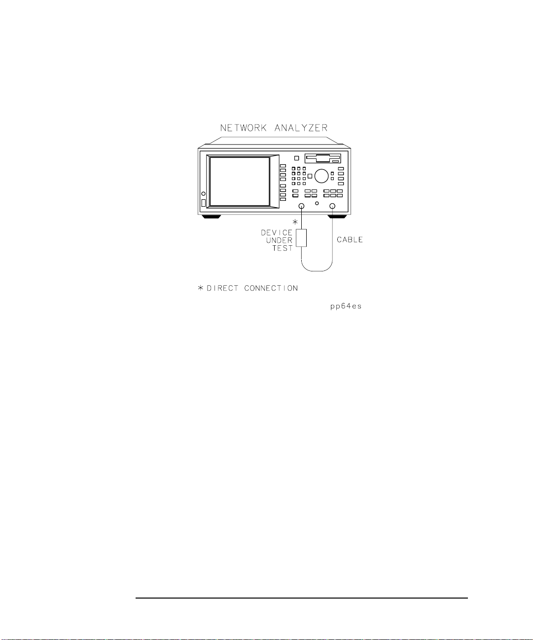
Making Measurements

Measuring Transmission Response

Connect the DUT.

Figure 3-5 Equipment Setup for a Transmission Response Measurement

3-20 ET User’s Guide

Making Measurements

Autoscale

Marker Search

Max Search

Mkr−> Max

Measuring Transmission Response

View and Interpret the Transmission Measurement Results.

1. To view the entire measurement trace on the display, press

2. To interpret the transmission measurement, refer to Figure 3-6,

“Example of a Transmission Response Measurement Display,” or your

analyzer's display if you are making this measurement on your instrument.

a. The values shown on the horizontal axis are the frequencies in

MHz. The values shown on the vertical axis are the power ratios in decibels (dB) of the transmitted signal through the device divided by the incident power. To display the result in logarithmic magnitude format (designated by "Log Mag" at the top of the measurement screen), the analyzer computes the measurement trace using the following formula:

trans



Transmission dB() 10 log

where P where P

b. A level of 0 dB would indicate a lossless through cable or device

(no loss or gain). Values greater than 0 dB indicate that the DUT has gain. Values less than 0 dB indicate loss.

= the power transmitted through the device and

trans

= the incident power.

inc

------------- -



inc

SCALE

3. To quickly determine the ﬁlter's minimum insertion loss, press

MARKER

4. Note the marker readout in Figure 3-6 provides the frequency and amplitude of the minimum insertion loss point.

ET User’s Guide 3-21

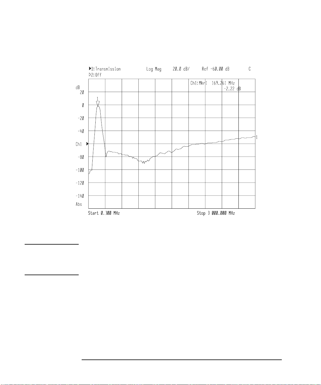
Making Measurements

Measuring Transmission Response

Figure 3-6 Example of a Transmission Response Measurement Display

5. See “Using Markers” on page 4-3 for more detailed information on using markers to interpret measurements.

NOTE For the measurement to be valid, input signals must fall within the

dynamic range of the analyzer. See Chapter 5, “Optimizing

Measurements,” for techniques to increase the dynamic range of the

analyzer.

3-22 ET User’s Guide

Making Measurements

More Cal

Cal Kit

Type-N(m)

Measuring Transmission Response

Calibrating for Noninsertable Devices

A noninsertable device is one that cannot be inserted in place of a zero-length through-standard. It has the same connectors on each port (type and sex) or has a different type of connector on each port (SMA on one port, and type-N on the other, for example). The following two calibration methods are available for noninsertable devices:

• swap equal adapters

• modify the calibration kit deﬁnition of the through standard In the following examples, the noninsertable device is type-N, with

female input and output connectors.

Method A: Swap Equal Adapters.

With this method, you use two precision matched adapters which are “equal.” To be equal, the adapters must have the same match, characteristic impedance (Z0), insertion loss, and electrical delay. The adapters in most HP/Agilent calibration kits have matched electrical lengths, even if the physical lengths appear different.

NOTE For analyzers with 50 ohm input impedance only: in the 50 ohm type-N

calibration kit (85032B), there are four equal adapters: two APC-7 to type-N(f), and two APC-7 to type-N(m). To create adapter A in the following example, connect an APC-7-to-type-N(f) adapter with an APC-7 to type-N(m) adapter. To create adapter B, connect two APC-7 to type-N(m) adapters.

NOTE By convention, cal kit labels in the analyzer indicate the sex of the port

with which they are used. For example, the default cal kit for the analyzer is type-N female because the front panel RF ports are female (the calibration standards, in turn, have male connectors).

1. Connect a test cable with type-N(m) connectors to the TRANSMISSION port.

2. To select a calibration kit for the REFLECTION port, press

, and use the front panel knob or the

keys to highlight the REFLECTION port in the display’s table.

Press .

3. Connect adapter A (type-N(m) to type-N(f)) to the REFLECTION port.

ET User’s Guide 3-23

CAL

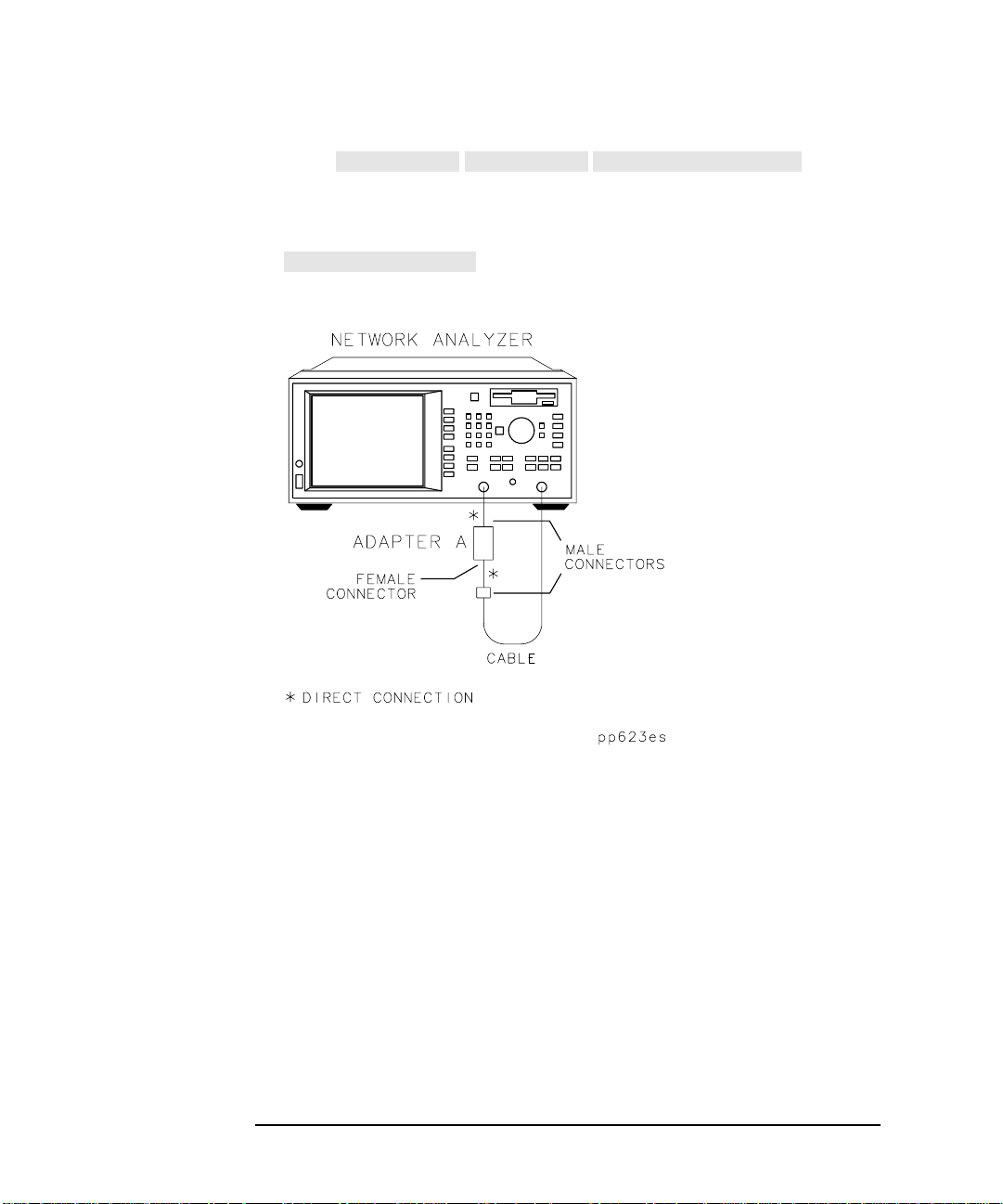
Making Measurements

Prior Menu

Enhanced Response

Measure Standard

Measuring Transmission Response

4. Press .

5. When the instrument prompts you to connect a through cable, connect the TRANSMISSION port test cable to adapter A on the REFLECTION port as shown in Figure 3-7. Press

Figure 3-7 Through-Cable Connection

6. Remove adapter A, and place adapter B (type-N(m) to type-N(m)) on the REFLECTION port. Adapter B becomes the effective test port.

7. When the instrument prompts you, connect three standards (open, short, and load) to adapter B—as shown in Figure 3-8.

3-24 ET User’s Guide

Figure 3-8 Open, Short, Load Connections

Measure Standard

Making Measurements

Measuring Transmission Response

NOTE Changing sweep frequencies (and other source parameters) may affect

8. Press after connecting each standard.

9. The analyzer will measure each standard and then calculate the new calibration coefﬁcients. The message "Calibration complete." will appear for a few seconds when the analyzer is done calculating the new error correction array.

your calibration. See Chapter 6 for more information.

ET User’s Guide 3-25

Making Measurements

Measuring Transmission Response

Connect the DUT.

10.Measure the test device with adapter B in place as shown in

Figure 3-9.

Figure 3-9 Equipment Setup for a Transmission Response Measurement of

a Noninsertable Two-Port Device

3-26 ET User’s Guide

Making Measurements

User Preset

Factory Preset

More Cal

Cal Kit

Type-N(m)

Reﬂection

Measuring Transmission Response

Method B: Modify the Calibration Kit Deﬁnition of the Through Standard.

With this method, it is only necessary to use one adapter. The DUT has type-N(f) input and output connectors. The calibration kit through-standard deﬁnition is modiﬁed to compensate for the adapter and then saved as a user kit. However, the electrical delay of the adapter must ﬁrst be found.

NOTE By convention, cal kit labels in the analyzer indicate the sex of the port

with which they are used. For example, the default cal kit for the analyzer is type-N female because the front panel RF ports are female (the calibration standards, in turn, have male connectors).

NOTE For analyzers with 50 ohm input impedance only: in the 50 ohm type-N

calibration kit (85032B), there are four equal adapters: two APC-7-to-type-N(f), and two APC-7-to-type-N(m). To create the adapter in the following example, connect two APC-7-to-type-N(f) adapters.

1. Connect a test cable with type-N(m) connectors to the REFLECTION port.

2. Connect a test cable with type-N(m) connectors to the TRANSMISSION port.

3. To select a calibration kit for the REFLECTION port, press

PRESET

highlight the REFLECTION port in the display’s table. Press

4. Press . Perform a one-port reﬂection calibration using type-N(f) standards on the type-N(m) open-end of the REFLECTION port test cable. Refer to “Perform a One-Port

Reﬂection Calibration” on page 3-34.

5. Connect the type-N female-to-female adapter to the type-N(m) openend of the REFLECTION port test cable.

6. Add a type-N(m) short to the open end of the adapter as shown in

Figure 3-10.

ET User’s Guide 3-27

( or )

, and use the front panel knob or the keys to

MEAS 1

CAL

Making Measurements

Delay

Marker Functions

Marker Math

Statistics

More Cal

Cal Kit

Type-N(f)

Measuring Transmission Response

Figure 3-10 Short Connection to the Adapter

7. Select the delay format for your measurement by pressing

FORMAT

8. Press to automatically select marker 1 as the active marker. Position marker 1 to the left edge of the measurement trace.

9. Press to select marker 2 as the active marker. Position marker 2 to the right edge of the measurement trace.

10.Press . Find the mean value, located in the upper right corner of the display.

11.Divide the mean value by 2. Record this value for use later in the procedure.

12.Select a type-N(f) calibration kit for the REFLECTION port. This is necessary because the type-N(m) short (connected to the adapter on port 2) is a component in a type-N(f) calibration kit. Press

Press .

3-28 ET User’s Guide

MARKER

keys to highlight the REFLECTION port in the display’s table.

CAL

, and use the front panel knob or the

Measuring Transmission Response

Operating Parameters

Next Screen

More Cal

Cal Kit

Type-N(m)

More Cal

Cal Kit

Modify Type-N(m)

Thru

Delay

Prior Menu

Mod Kit SaveRecall

Save

Add Kit Description

Select Char

Enter

Enhanced Response

13.Determine the offset delay of the calibration short:

Making Measurements

• Press

• Press until the Cal Kit screen is displayed.

• In the “CAL KIT: Type N(m)” display, ﬁnd the numeric value for the delay of the short.

14.Subtract this value from the value calculated in Step 11. This corresponds to the delay of the adapter.

15.Remove the short from the adapter.

16.Reselect a type-N(m) calibration kit for the REFLECTION port. This is necessary because the type-N(m) short has been removed from the adapter. Press , and use the front panel knob or the keys to highlight the REFLECTION port in the display’s table. Press .

17.Modify the calibration kit deﬁnition of the through-standard by entering the electrical delay of the adapter. To do so:

• Press

18.Save (and automatically assign) the modiﬁed cal kit buffer as a user-deﬁned cal kit for the REFLECTION port. To do so:

• Press . Use the front panel

knob or the keys to highlight the desired User Kit in the display’s table. (In this example, highlight Cal Kit A.) Press

SYSTEM OPTIONS

CAL

. Enter the delay value with the keypad and softkeys.

If you want to enter a cal kit description in the display’s table, press . Use a keyboard connected to the analyzer’s DIN KEYBOARD connector to enter the description. (If you don’t have a keyboard, you can use the analyzer’s

keys or the front panel knob and the key to select and enter characters from the top of the analyzer’s display. Press when done.)

19.Start the calibration process by pressing

CAL

ET User’s Guide 3-29

MEAS 1

Transmissn

Making Measurements

Measure Standard

Measuring Transmission Response

20.When the instrument prompts you, connect three standards (open, short, and load) to the REFLECTION port test cable as shown in

Figure 3-11.

21.Press after connecting each standard.

Figure 3-11 Open, Short, Load Connections

3-30 ET User’s Guide

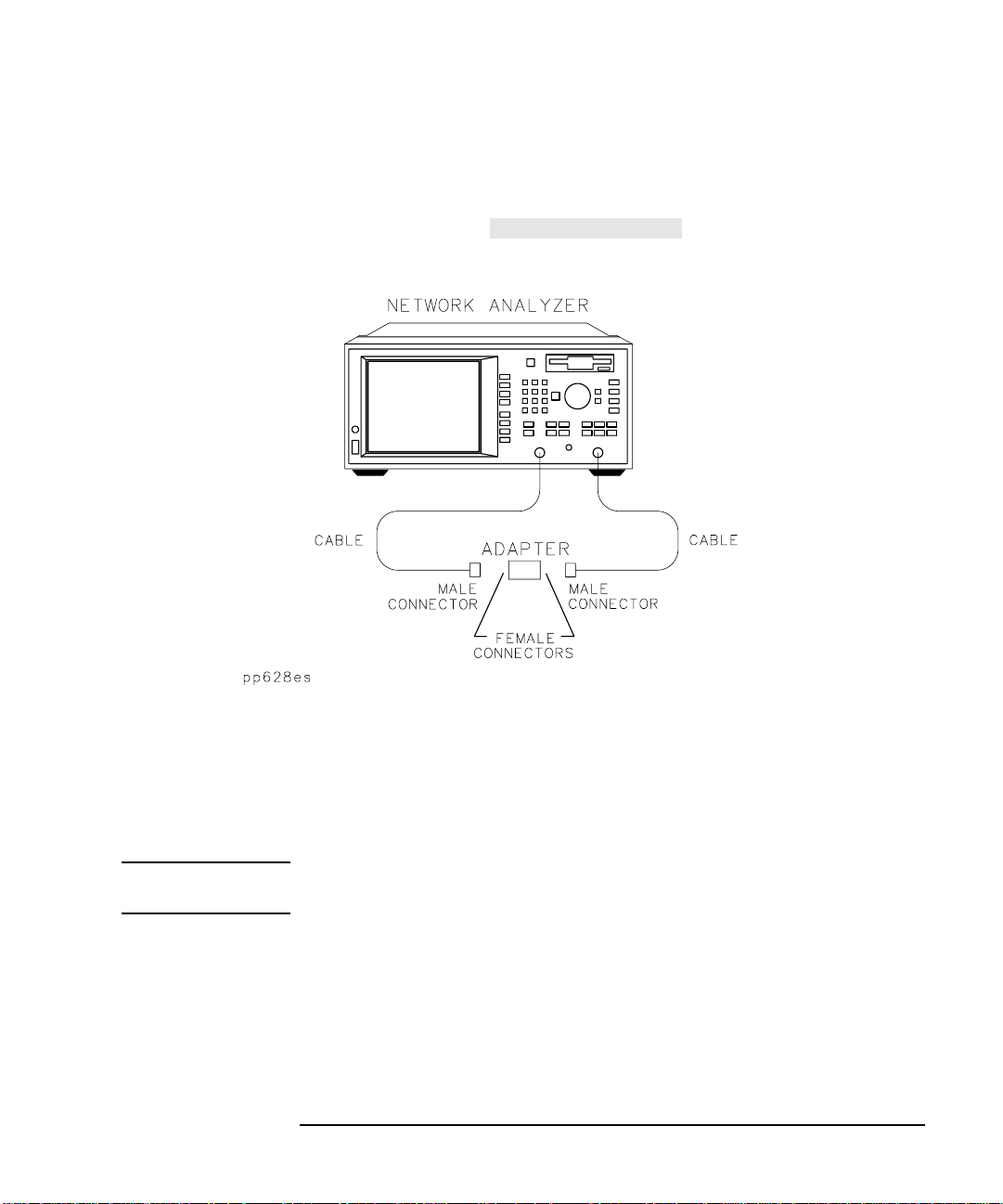
22.When the instrument prompts you to connect a through cable, insert

Measure Standard

the female-to-female adapter between the test cables connected to the REFLECTION port and the TRANSMISSION port as shown in

Figure 3-12. Press .

Figure 3-12 Through-Cable Connection

Making Measurements

Measuring Transmission Response

NOTE Changing sweep frequencies (and other source parameters) may affect

23.The analyzer will measure each standard and then calculate new calibration coefﬁcients. The message "Calibration complete." will appear for a few seconds when the analyzer is done calculating the new error correction array.

24.Remove the adapter between the test cables connected to the REFLECTION port and the TRANSMISSION port.

your calibration. See Chapter 6 for more information.

ET User’s Guide 3-31

Making Measurements

Measuring Transmission Response

Connect the DUT.

25.Measure the test device using the setup shown in Figure 3-13.

Figure 3-13 Equipment Setup for a Transmission Response Measurement of

a Type-N(f) Two-Port Noninsertable Device

3-32 ET User’s Guide

Making Measurements

User Preset

Factory Preset

Reﬂection

Measuring Reﬂection Response

This section uses an example measurement to describe how to calibrate for and make a basic reﬂection response measurement. In this example, a user-deﬁned one-port calibration is used. See the table below for a list of all possible calibration choices for a reﬂection response measurement.

TIP An optimum calibration is critical for achieving best measurement

accuracy. Refer to Chapter 6, “Calibrating for Increased Measurement

Accuracy,” for detailed information about all of the various aspects of

calibration.

Table 3-3 Calibration Choices for a Reﬂection Response Measurement

Measurement Type Calibration Choices

Reﬂection Default 1-Port

1-Port

In this example, a bandpass ﬁlter like the one that was supplied with your network analyzer is used.

NOTE This example measurement uses the default instrument parameters for

Enter the Measurement Parameters

Press the following keys on the analyzer:

PRESET

( or )

MEAS 1

a reﬂection response measurement. If your particular reﬂection measurement requires speciﬁc parameters (such as frequency range, source power level, number of data points, and sweep time), enter them now.

ET User’s Guide 3-33

Making Measurements

Measuring Reﬂection Response

Perform a One-Port Reﬂection Calibration

A one-port reﬂection calibration uses known standards to correct for directivity, source match, and frequency response errors when using narrowband detection. When you perform a one-port reﬂection calibration, the analyzer performs correction at each data point across the selected frequency band. The default number of data points per sweep is 201, but you can select any number between 3 and 1601. Interpolation recalculates the error correction array for reduced frequency spans. If the frequency span is increased, the calibration is invalidated, and the default one-port calibration is automatically restored.

To perform a one-port reﬂection calibration, you will need one of the following calibration kits depending on the nominal impedance of your analyzer:

Cal Kit Model

Number

85038M 50 Ω 7-16 ✓

Impedance

Connector

Type

For Use with Male Test Ports

For Use

with Female

Test Ports

3-34 ET User’s Guide

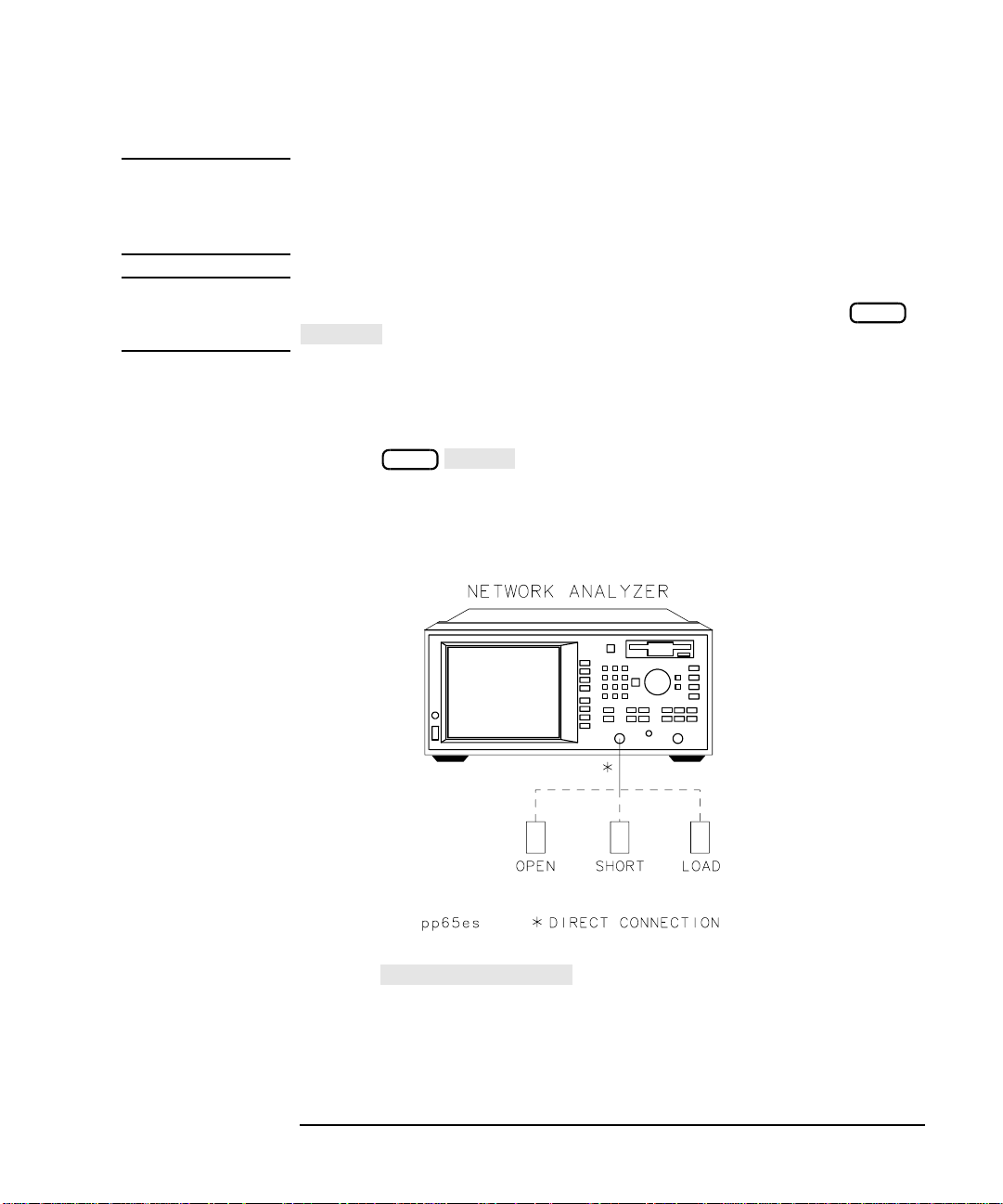
Making Measurements

Cal Kit

1-Port

Measure Standard

Measuring Reﬂection Response

NOTE By convention, cal kit labels in the analyzer indicate the sex of the port

with which they are used. For example, the default cal kit for the analyzer is type-N female because the front panel RF ports are female (the calibration standards, in turn, have male connectors).

NOTE If you are going to be using calibration standards other than the default

(female type-N), you must select the connector type by pressing

and then selecting the appropriate type.

Chapter 6 provides detail about when this calibration is necessary. If you

wish to perform a one-port reﬂection calibration on your instrument for a reﬂection response measurement, execute the following steps:

CAL

1. Press .

2. The instrument will prompt you to connect three standards (open, short and load) and measure them. See Figure 3-14.

Figure 3-14 Open, Short, Load Connections

3. Press after connecting each standard.

CAL

4. The analyzer will measure each standard and then calculate new calibration coefﬁcients. The message "Calibration complete." will appear for a few seconds when the analyzer is done calculating the new error correction array.

ET User’s Guide 3-35

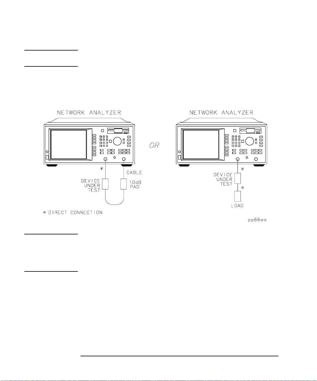
Making Measurements

Measuring Reﬂection Response

NOTE Changing sweep frequencies (and other source parameters) may affect

your calibration. See Chapter 6 for more information.

Connect the DUT

Figure 3-15 Equipment Setup for a Reﬂection Measurement of a Two-Port

Device

NOTE If you connect the DUT between both analyzer ports, it is recommended

that you use a 10 dB pad on the output of the DUT to improve measurement accuracy. If you connect a two-port DUT to the REFLECTION port only, it is recommended that you use a high-quality load (such as a calibration standard) on the output of the DUT.

3-36 ET User’s Guide

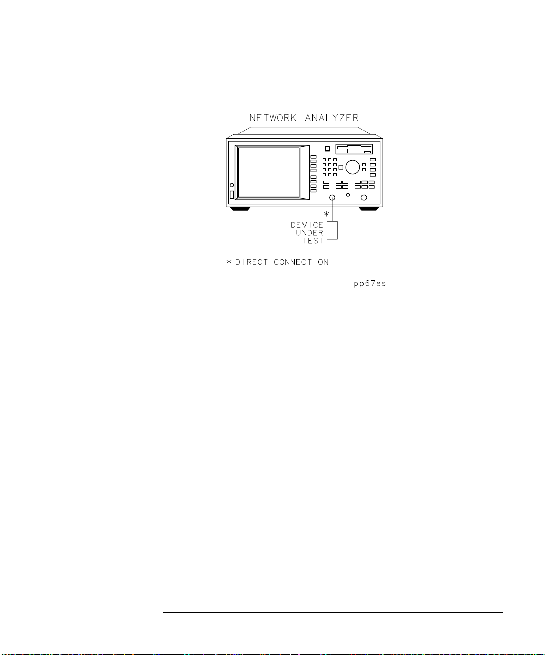
Making Measurements

Measuring Reﬂection Response

Figure 3-16 Equipment Setup for a Reﬂection Measurement of a One-Port

Device

ET User’s Guide 3-37

Making Measurements

Autoscale

Measuring Reﬂection Response

View and Interpret the Reﬂection Measurement Results

1. To view the entire measurement trace on the display, press ,

2. To interpret the reﬂection measurement, refer to Figure 3-17,

“Example of a Reﬂection Measurement Display,” or your analyzer's

display if you are making this measurement on your instrument. a. The values shown on the horizontal axis are the frequencies in

MHz. The values shown on the vertical axis are the power ratios in decibels (dB) of the reﬂected signal divided by the incident power. To display the result in logarithmic magnitude format (designated by Log Mag at the top of the measurement screen), the analyzer computes the measurement trace using the following formula:

refl



Reflection dB() 10 log

where P where P

b. A level of 0 dB indicates that all of the power applied to the DUT is

reﬂected back, and that none of it passes through the DUT or is absorbed by the DUT.

c. Values less than 0 dB indicate that power is either absorbed or

transmitted by the DUT. Although they are not typically seen, values greater than 0 dB do occur under certain circumstances such as when the measurement needs to be enhanced by calibration, or when the device is active (an ampliﬁer for instance) and perhaps oscillating.

= the power of the signal reﬂected from the device and

reﬂ

= the incident power.

inc

----------



inc

SCALE

3-38 ET User’s Guide

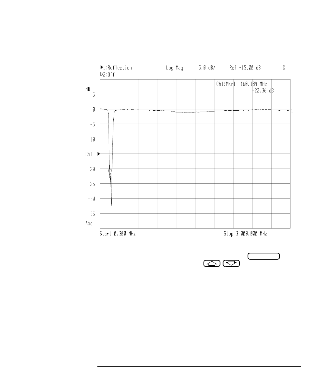
Measuring Reﬂection Response

Figure 3-17 Example of a Reﬂection Measurement Display

Making Measurements

3. To quickly determine the ﬁlter's return loss, press and then use the front panel knob, the keys, or the numeric keypad to read the value of return loss at the desired frequency.

4. See “Using Instrument Functions” on page 4-1 for detailed information on using markers to interpret measurements.

ET User’s Guide 3-39

MARKER

Making Measurements

Detection Options

Narrowband Internal

Making a Power Measurement using Broadband Detection

Power measurements can be made using either narrowband or broadband detection. The example in this section is of a broadband power measurement. If you are only interested in the output power of your device at the same frequency as the analyzer's source, you can select for a narrowband-detection power measurement. A narrowband-detection power measurement only measures the power within the tuned receiver's bandwidth, centered at the source frequency.

When you measure a device for absolute output power, the network analyzer uses the broadband detection mode and measures the total power of all frequencies present in the transmitted signal (B*). This signal may contain frequencies other than the source frequency such as when the DUT is a mixer.

This section uses an example measurement to describe how to normalize the data and measure the total output power of an ampliﬁer.

MEAS 1

NOTE Broadband power measurements are only speciﬁed for measurements

with a start frequency of ≥10 MHz.

3-40 ET User’s Guide

Making Measurements

User Preset

Factory Preset

Power

Making a Power Measurement using Broadband Detection

Enter the Measurement Parameters

Press the following keys on the analyzer:

PRESET

( or )

MEAS 1

NOTE This example measurement uses the default instrument parameters for

a power measurement. If your particular power measurement requires different parameters (such as source power level, number of data points, and sweep time), enter them now.

CAUTION Damage to your analyzer will occur if the receiver input power exceeds

+20 dBm or ±30 Vdc. The analyzer's source cannot signiﬁcantly exceed this level, however if your DUT has gain, then attenuation on the analyzer’s RF IN port may be necessary. See “Attenuation and

Ampliﬁcation in a Measurement Setup” on page 3-8 for more

information.

ET User’s Guide 3-41

Making Measurements

Start

MHz

Normalize

Normalize on OFF

Making a Power Measurement using Broadband Detection

Perform a Normalization Calibration

Normalization is the simplest type of calibration. The analyzer stores a measurement trace into memory and divides subsequent measurements by the stored data to remove unwanted frequency response errors. This calibration is used for the power measurement to remove the insertion-loss error of the test cable. Changing the frequency span or number of measurement points will invalidate a normalization calibration.

Execute the following steps to perform a normalization calibration:

1. Connect the equipment as shown in Figure 3-18.

Figure 3-18 Through-Cable Connection

2. Set the following frequency parameters:

FREQ

3. Press or . This stores the data into memory and divides subsequent

measurements by the stored data to remove frequency response errors.

3-42 ET User’s Guide

DISPLAY

CAL

Making a Power Measurement using Broadband Detection

4. Insert the ampliﬁer as shown in Figure 3-19.

Connect the DUT

Figure 3-19 Equipment Setup for a Power Measurement

Making Measurements

ET User’s Guide 3-43

Making Measurements

Autoscale

Making a Power Measurement using Broadband Detection

View and Interpret the Power Measurement Results

1. To view the measurement trace, press .

2. To interpret the power measurement, refer to Figure 3-20 or your analyzer's display if you are making this measurement on your instrument.

a. When making a power measurement, the display shows the power

measured at the analyzer's RF IN connector. This power is absolute power, as opposed to a power ratio.

b. Note that when making a power measurement, the values

associated with the vertical axis are in units of dBm, which is the power measured in reference to 1 mW.

• 0 dBm = 1 mW

• −10 dBm = 100 µW

• +10 dBm = 10 mW Other units available for a power measurement include dBW,

dBµW, W, mW, and µW.

SCALE

3-44 ET User’s Guide

Making a Power Measurement using Broadband Detection

Figure 3-20 Example of a Power Measurement

Making Measurements

CAUTION If the analyzer's RF output power level is set to higher than the speciﬁed

output power for your analyzer, the source could go unleveled. See

Chapter 9, “Speciﬁcations,” for source and receiver speciﬁcations. If your

device requires input power greater than your analyzer's speciﬁed output power, you may need to use a preampliﬁer in your measurement setup. However, remember to not exceed the receiver damage limit of +20 dBm.

ET User’s Guide 3-45

Making Measurements

Measuring Conversion Loss

Conversion loss is the ratio of IF output power to RF input power expressed in dB. This section uses an example measurement to describe how to measure the conversion loss of a broadband mixer.

When characterizing a device's conversion loss, the analyzer uses broadband detection to compare the transmitted signal (B*) to the reference signal (R*). This is because the input and output signals of a frequency-translating device may be different. Since broadband detection measures signals at all frequencies, you may want to use a ﬁlter to remove unwanted signals such as LO feedthrough when performing this measurement.

For example, an RF signal at 900 MHz mixed with an LO signal at 200 MHz, results in mixing products at 700 MHz and 1100 MHz, as well as the original 900 MHz and 200 MHz RF and LO signals.

Figure 3-21 Filtering Out the Unwanted Mixing Products

3-46 ET User’s Guide

Making Measurements

User Preset

Factory Preset

Conversion Loss

Measuring Conversion Loss

Inserting a 700 MHz bandpass ﬁlter in the measurement setup removes the unwanted signals at 200 MHz, 900 MHz, and 1100 MHz, providing an accurate measurement of the desired IF signal at 700 MHz.

In the following example, the conversion loss of a mixer will be measured with RF input frequencies over a 15 MHz span centered at 900 MHz. With an LO frequency of 200 MHz, the mixer IF frequency will sweep over a 15 MHz span centered at 700 MHz.

Enter the Measurement Parameters

Press the following keys on the analyzer:

PRESET

( or )

MEAS 1

NOTE This example measurement uses the default instrument parameters for

a conversion loss measurement. If your particular conversion loss measurement requires different parameters (such as source power level, number of data points, and sweeptime), enter them now.

Perform a Normalization Calibration

Normalization is the simplest type of calibration. The analyzer stores a measurement trace into memory and divides subsequent measurements by the stored data to remove unwanted frequency-response errors. This calibration is used for this measurement to remove the insertion loss errors of the IF ﬁlter and the interconnect cables. Changing the frequency span or number of measurement points will invalidate a normalization calibration.

Perform the following steps to perform a normalization calibration:

1. Connect the equipment as shown in Figure 3-22.

ET User’s Guide 3-47

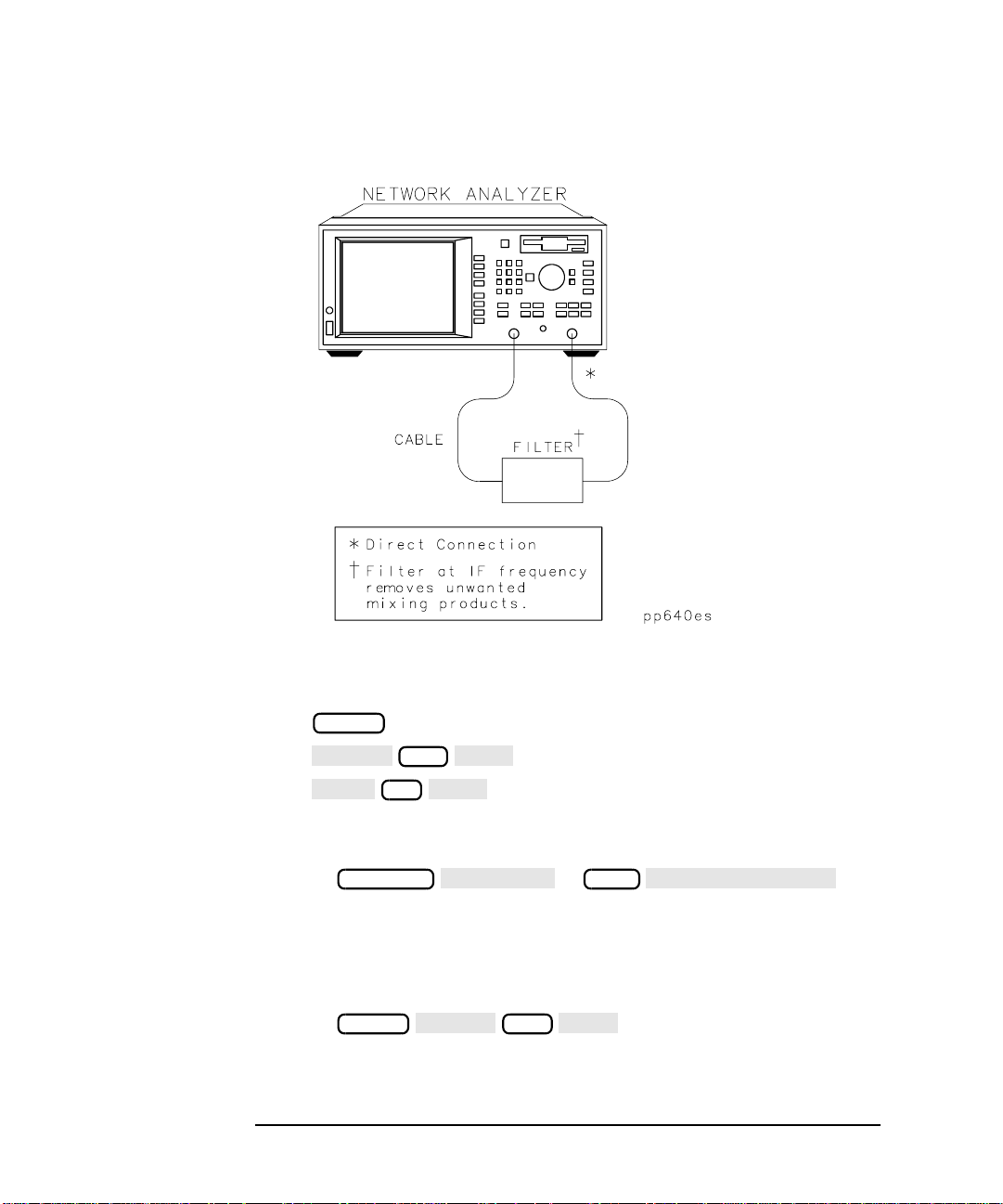
Making Measurements

Center

700

MHz

Span

MHz

Normalize

Normalize on OFF

Center

MHz

Measuring Conversion Loss

Figure 3-22 Through-Cable Connection

2. Set the following frequency parameters:

FREQ

This sets the analyzer frequency range to sweep over the passband of the IF ﬁlter (700 MHz).

3. Press or . This stores the ﬁlter response passband into memory, and sets up a

normalized trace so that the ﬁlter response magnitude is removed from the measurement.

4. Insert the mixer as shown in Figure 3-23.

5. Press to change the center frequency so that the mixing product of the mixer is in the passband of the IF ﬁlter.

3-48 ET User’s Guide

DISPLAY

FREQ

CAL

900

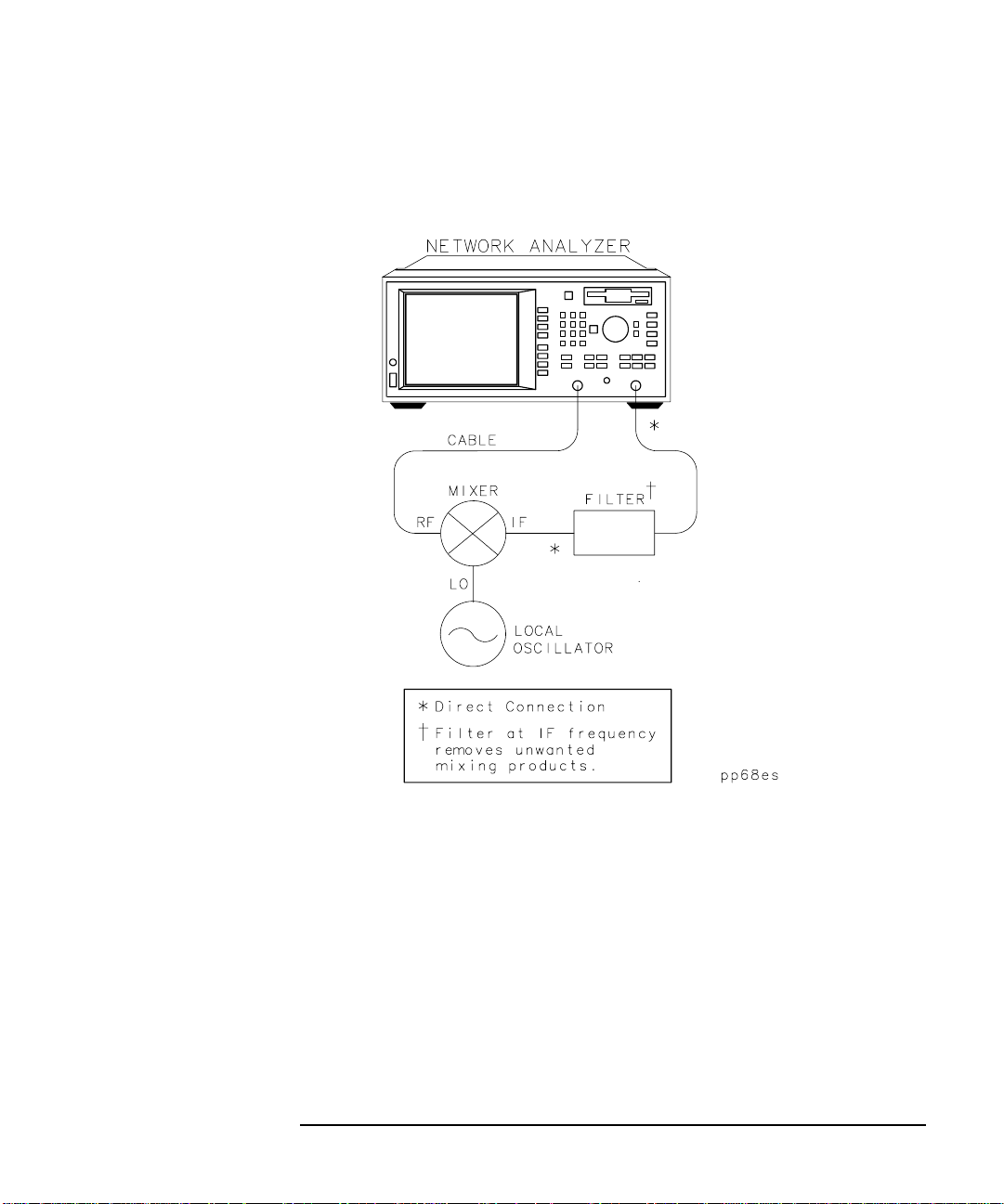
Making Measurements

Measuring Conversion Loss

Connect the DUT

Figure 3-23 Equipment Setup for a Conversion Loss Measurement

ET User’s Guide 3-49

Making Measurements

Autoscale

Marker Search

Max Search

Mkr−> Max

Measuring Conversion Loss

View and Interpret the Conversion Loss Results

1. If necessary to view the measurement trace, press

2. To interpret the conversion loss measurement, refer toFigure 3-24 or your analyzer's display if you are making this measurement on your instrument.

a. The values shown on the horizontal axis represent the source RF

output. The values shown on the vertical axis are the power ratio in decibels (dB) of the transmitted signal through the device divided by the incident power. To display the result in logarithmic magnitude format (designated by Log Mag at the top of the measurement screen), the analyzer computes the measurement trace using the following formula:

Conversion Loss dB() 10 log

where P and where P

b. A level of 0 dB would indicate a perfect device (no loss or gain).

Values greater than 0 dB indicate that the mixer has gain. Values less than 0 dB indicate mixer conversion loss.

3. If you wish, you can quickly determine the mixer's minimum conversion loss by pressing

= the power measured at the IF output of the mixer

trans

= the incident power at the RF input.

inc

MARKER

SCALE

trans



------------- -



inc

3-50 ET User’s Guide

Figure 3-24 Example of a Conversion Loss Measurement

Making Measurements

Measuring Conversion Loss

NOTE For the measurement to be valid, input signals must fall within the

dynamic range and frequency range of the analyzer. See Chapter 5 for techniques to increase the dynamic range of the analyzer.

ET User’s Guide 3-51

Agilent 8712ET User Manual

Specifications and Main Features

Frequently Asked Questions

User Manual

Introducing the Analyzer

1 Installing the Analyzer

Introduction

Step 1. Check the Shipment

Step 2. Meet Electrical and Environmental Requirements

Step 3. Check the Analyzer Operation

Connecting Peripherals and Controllers

Installing the Analyzer in a Rack

Preventive Maintenance

Clean the Display Use a soft cloth and, if necessary, a mild cleaning solution to clean the

Check the RF Front Panel Connectors

2 Getting Started

Introduction

Front Panel Tour

Entering Measurement Parameters

Presetting the Analyzer

Entering Frequency Range

Entering Source Power Level

Scaling the Measurement Trace

Entering Active Measurement Channel and Measurement Type

Viewing Measurement Channels

Performing the Operator's Check

Equipment List

Make a Transmission Measurement

Make a Broadband Power Measurement

If the Analyzer Fails the Operator's Check

3 Making Measurements

Introduction

Measuring Devices with Your Network Analyzer

When to Change the System Impedance

The Typical Measurement Sequence

Using the BEGIN Key to Make Measurements

BEGIN Key Overview

AUTOST Files

The User BEGIN Function

Measuring Transmission Response

Enter the Measurement Parameters

Perform an Enhanced Response Calibration

Enter the Measurement Parameters

Connect the DUT

Making a Power Measurement using Broadband Detection

Enter the Measurement Parameters

Perform a Normalization Calibration

Connect the DUT

View and Interpret the Power Measurement Results

Measuring Conversion Loss

Enter the Measurement Parameters

Perform a Normalization Calibration

Connect the DUT

View and Interpret the Conversion Loss Results