Agilent 86030A Users Guide

Download

User’s Guide

Agilent Technologies 86030A Lightwave Component Analyzer System

Agilent Technologies Part No. 86030-90001 Printed in USA April 2000

Agilent Technologies, Inc. Lightwave Division 1400 Fountaingrove Parkway Santa Rosa, CA 95403-1799, USA (707) 577-1400

Notice.

The information contained in this document is subject to change without notice. Companies, names, and data used in examples herein are fictitious unless otherwise noted. Agilent Technologies makes no warranty of any kind with regard to this material, including but not limited to, the implied warranties of merchantability and fitness for a particular purpose. Agilent Technologies shall not be liable for er rors contained herein or for incidental or consequential damages in connection with the furnishing, performance, or use of this material.

Restricted Rights Legend.

Use, duplication, or disclosure by the U.S. Government is subject to restrictions as set forth in subparagraph (c) (1) (ii) of the Rights in Technical Data and Computer Software clause at DFARS 252. 227-7013 for DOD agencies, and subparagraphs (c) (1) and (c) (2 ) of the Commercial Computer

Software Restricted Rights clause at FAR 52.227-1 9 for other agencies.

Warranty.

This Agilent Technologies instrument product is warranted against defects in material and workmanship for a period of one year from date of shipment. During the warranty period, Agilent Technologies Company will, at its option, either repair or replace products which prove to be defective. For warranty service or repair, this product must be returned to a service facility designated by Agilent Technologies. Buyer shall prepay shipping charges to Agilent Technologies and Agilent Technologies shall pay shipping charges to return the product to Buyer. However, Buyer shall pay all shipping charges, duties, and taxes for products returned to Agilent Technologies from another country.

Agilent Technologies warrants that its software and firmware designated by Agilent Technologies for use with an instrument will execute its programming instructions when properly installed on that instrument. Agilent Technologies does not warrant that the operation of the instrument, or sof tware, or firmware will be uninterrupted or errorfree.

Limitation of Warranty.

The foregoing warranty shall not apply to defects resulting from improper or inadequate maintenance by Buyer, Buyersupplied software or interfacing, unauthorized modification or misuse, operation outside of the environmental

specifications for the product, or improper site preparation or maintenance.

No other warranty is expressed or implied. Agilent Technologies specifically disclaims the implied warranties of merchantability and fitness for a particular purpose.

Exclusive Remedies.

The remedies provided herein are buyer's sole and exclusive remedies. Agilent Technologies shall not be liable for any direct, indirect, special, incidental, or consequential damages, whether based on contract, tort, or any other legal theory.

Safety Symbols.

CAUTION

The caution sign denotes a hazard. It calls attention to a procedure which, if not correctly performed or adhered to, could result in damage to or destruction of the product. Do not proceed beyond a caution sign until the indicated conditions are fully understood and met.

WARNING

The warning sign denotes a hazard. It calls attention to a procedure which, if not correctly performed or adhered to, could result in injury or loss of life. Do not proceed beyond a warning sign until the indicated conditions are fully understood and met.

The instruction manual symbol. The product is marked with this warning symbol when it is necessary for the user to refer to the instructions in the manual.

The laser radiation symbol. This warning symbol is marked on products which have a laser output.

The AC symbol is used to indicate the required nature of the line module input power.

| The ON symbols are used to mark the positions of the instrument power line switch.

❍The OFF symbols are used to mark the positions of the instrument power line switch.

The CE mark is a registered trademark of the European Community.

The CSA mark is a registered trademark of the Canadian Standards Association.

The C-Tick mark is a registered trademark of the Australian Spectrum Management Agency.

This text denotes the

ISM1-A

instrument is an Industrial Scientific and Medical Group 1 Class A product.

Software License

The following License Terms govern your use of the accompanying Software unless you have a separate signed agreement with Agilent.

License Grant. Agilent grants you a license to Use one copy of the Software. “Use” means storing, loading, installing, executing or displaying the Software. You may not modify the Software or disable any licensing or control features of the Software. If the Software is licensed for “concurrent use,” you may not allow more than the maximum number of authorized users to Use the Software concurrently.

Ownership. The Software is owned and copyrighted by Agilent or its third party suppliers. Your license confers no title to, or ownership in, the Software and is not a sale of any rights in the Software. Agilent’s third party suppliers may protect their rights in the event of any violation of these License Terms.

Copies and Adaptations. You may only make copies or adaptations of the Software for archival purposes or when copying or adaptation is an essential step in the authorized Use of the Software. You must reproduce all copyright notices in the original Software on all copies or adaptations. You may not copy the Software onto any public network.

No Disassembly or Decryption. You may not disassemble or decompile the Software unless Agilent’s prior written consent is obtained. In some jurisdictio ns, Agilen t’s consent may not be required for limited disassembly or decompi-

lation. Upon request, you will provide Agilent with reasonably detailed information regarding any disassembly or decompilation. You may not decrypt the Software unless decryption is a necessary part of the operation of the Software.

Transfer. Your license will automatically terminate upon any transfer of the Software. Upon transfer, you must deliver the Software, including any copies and related documentation, to the transferee. The transferee must accept these License Terms as a condition of the transfer.

Termination. Agilent may terminate your license upon notice for failure to comply with any of these License Terms. Upon termination, you must immediately destroy the Software, together with all copies, adaptations and merged portions in any form.

Export Requirements. You may not export or re-export the Software or any copies or adapt ation in violatio n of any applicable laws or regulations.

U.S. Government Restricted Rights. The Software and Documentation have been developed entirely at private expense. They are delivered and licensed as “commercial computer software” as defined in DFARS 252.227-7013 (Oct

1988), DFARS 252.211-7015 (May 1991) or DFARS

252.227-7014 (Jun 1995), as a “commercial item” as defined in FAR 2.101(a), or as “Restricted computer software” as defined in FAR

52.227-19 (Jun 1987) (or any equivalent agency regulation or contract clause), whichever is applicable. You have those

rights provided for such Software and Documentation by the applicable FAR or DFARS clause or the Agi lent standard software agreement for the product involved.

Limited Software Warranty

Software. Agilent Technologies warrants for a period of one year from the date of purchase that the software product will execute its programming instructions when properly installed on the instrument indicated on this package. Agilent Technologies does not warrant that the operation of the software will be uninterrupted or error free. In the event that this software product fails to execute its programming instructions during the warranty period, Customer’s remedy shall be to return the media to Agilent Technologies for replacement. Should Agilent Technologies be unable to replace the media within a reasonable amount of time, Customer’s alternate remedy shall be a refund of the purchase price upon return of the product and all copies.

Media. Agilent Technologies warrants the media upon which this product is recorded to be free from defects in materials and workmanship under normal use for a period of one year from the date of purchase. In the event any media prove to be defective during the warranty period, Customer’s remedy shall be to return the media to Agilent Technologies for replacement. Should Agilent Technologies be unable to replace the media within a reasonable amount of time, Customer’s alternate remedy shall be a

refund of the purchase price upon return of the product and all copies.

Notice of Warranty Claims. Customer must notify Agilent Technologies in writing of any warranty claim not later than thirty (30) days after the expiration of the warranty period.

Limitation of Warranty. Agilent Technologies makes no other express warranty, whether written or oral, with respect to this product. Any implied warranty of merchantability or fitness is limited to the one year duration of this written warranty.

This warranty gives specific legal rights, and Customer may also have other rights which vary from state to state, or province to province.

Exclusive Remedies. The remedies provided above are Customer’s sole and exclusive remedies. In no event shall Agilent Technologies be liable for any direct, indirect, special, inci dental, or consequential damages (including lost profit) whether based on warranty, contract, tort, or any other legal theory.

Warranty Service. Warranty service may be obtained from the nearest Agilent Technologies sales office or other location indicated in the owner’s manual or service booklet.

iii

General Safety Considerations

This product has been designed and tested in accordance with IEC Publication 1010, Safety Requirements for Electronic Measuring Apparatus, and has been supplied in a safe condition. The instruction documentation contains information and warnings which must be followed by the user to ensure safe operation and to maintain the product in a safe condition.

WARNING If this product is not used as specified, the protection provided by the

equipment could be impaired. This product must be used in a normal condition (in which all means for protection are intact) only.

WARNING No operator serviceable parts inside. Refer servicing to qualified

personnel. To prevent electrical shock, do not remove covers.

General Safety Considerations iv

1 Getting Started

Configuration Options 1-6 Front Panel Features 1-8 Rear Panel Features 1-11 Software Overview 1-12 File Menu 1-13 Options Menu 1-20 Tools Menu 1-27 Laser Safety Considerations 1-30 Accurate Measurements 1-33 Electrostatic Discharge Information 1-43 Quick Start 1-46

2 Measurement Techniques

The Calibrations 2-2 O/O Response and Isolation Bandwidth Calibration 2-5 O/E Response and Isolation Bandwidth Calibration 2-8 O/E Response and Match Bandwidth Calibration 2-11 E/O Response and Isolation Bandwidth Calibration 2-20 Agilent 86030A System Example Measurements 2-24 Electrical Mismatch Ripple and its Effects on Measurements. 2-25 Magnitude Response and Deviation From Linear Phase of a Lightwave Receiver 2-37 O/E RF Overload Detection Measurement 2-47

3 Theory of Operation

System Operation 3-2 Lightwave Test Set Operation 3-3 Measurement Calibration 3-6 O/O Measurement Calibration 3-7 O/E Measurement Calibration 3-9 E/O Measurement Calibration 3-11 Electrical Measurement Calibration 3-13 O/E Display Scaling Calculations 3-14 E/O Display Scaling Calculations 3-15

Contents-1

Contents

O/O Display Scaling Calculations 3-16

4 Installation

Installation 4-2 Step 1. Prepare the site 4-4 Step 2. Install the monitor mount assembly 4-6 Step 3. Install the keyboard/mouse transmitter and the work surface 4-8 Step 4. Confirm front and rear panel connections 4-9 Step 5. Turn the system on 4-11

5 System Verification

Lightwave Verification 5-3 If the Lightwave Verification Test Fails 5-7

6 Maintenance

86032A Test Set Troubleshooting Diagnostics 6-6 Verifying the RF Path Integrity of the 86032A 6-12 Modulator Troubleshooting Tips 6-16 Agilent Technologies Support and Maintenance 6-17 Electrostatic Discharge Information 6-19 Returning the System for Service 6-22 Agilent Technologies Sales and Service Offices 6-25 After Repair 6-26

7 Specifications and Regulatory Information

General Specifications 7-3 Electrical Specifications 7-4 Optical to Optical (O/O) Specifications 7-6 Optical to Electrical (O/E) Specifications 7-7 Electrical to Optical (E/O) Specifications 7-12 Characteristics 7-16 Optical to Electrical (O/E) Characteristics 7-18 Electrical to Optical (E/O) Characteristics 7-21 Regulatory Information 7-24 Declaration of Conformity 7-25

Contents-2

“Front Panel Features” on page 1-8 “Rear Panel Features” on page 1-11 “Software Overview” on page 1-12 “File Menu” on page 1-13 “Options Menu” on page 1-20 “Tools Menu” on page 1-27 “Laser Safety Considerations” on page 1-30 “Accurate Measurements” on page 1-33 “Electrostatic Discharge Information” on page 1-43 “Quick Start” on page 1-46

Getting Started

System Overview

The Agilent 86030A 50 GHz lightwave component analyzer provides accurate and repeatable characterization of electro-optical, optical, and electrical components.

Components such as O/E photodiode receivers, E/O photodiodes, lightwave modulators, and other optical and electrical components used in 40 Gb/s lightwave systems can be characterized in either a research and development or manufacturing environment.

The Agilent 86030A system consists of an Agilent 85107B vector network analyzer system, an 86032A 50 GHz lightwave test set, system software, and a personal computer serving as the system controller.

1-2

Getting Started

System Overview

1-3

Getting Started

System Overview

Calibrated Measurements

One of the key benefits of the 50 GHz lightwave component analyzer is its ability to perform calibrated measurements of optical components. The system contains an O/E receiver that has been factory calibrated in magnitude, and characterized in phase. The ability to make calibrated measurements assures accuracy, reliability, and confidence in the components being measured. Additionally, the laser source, optical modulator, and calibrated O/E receiver are temperature stabilized which also improves the accuracy and repeatability of measurements.

Verification Device

A verification device is included with the system. It consists on an Agilent 83440D O/E photodetector and its associated amplitude and phase data. This verification device can be used at any time to verify the measurement integrity of your system. A guided verification routine is provided which measures the verification device, and displays a graph of its response versus acceptable tolerances. The verification device can be used periodically to monitor system calibration, and indicate when the optical test set needs to be recalibrated. It can also be used to resolve uncertainty if unexpected results are obtained from a test device. This verification capability provides confidence in the measurement integrity of the system.

Measurement Software

Guided measurement software provides an easy-to-use operator interface. It provides pictorial diagrams of interconnections for configuration, calibration, and measurements. On-screen prompts also guide you through the entire measurement process, from the calibration to the measurement.

Data Management

Display, analysis, and archiving of data is easy and straightforward with the system. The measured data is displayed on the Agilent 8510C network analyzer. Full use of the analyzer’s functions such as markers, data formats, and data scaling features are available. Data can be archived to disk in either ASCII text or Microsoft Excel formats. The include Excel software allows data to be displayed and analyzed using standard Excel features and formats. Data connectivity to a local area network (LAN) is provided via a LAN card in the system’s PC.

1-4

Accessories Supplied

The accessories described below are shipped with your system.

Table 1-1. System Accessories

Description Agilent Model/Part Number Quantity

86030A Verification Kit

0 to 32 GHz Light Wave Detector 83440D 1

Cable Assembly 86030-60005 1

Power Supply 87421A 1

Reference Reflector Cable Assembly 81000BR 1

System Software Disk Set 86030-10001 1

Fiber Optic 4M Cable 1005-0173 3

Getting Started

System Overview

BNC Termination 1250-0207 2

6 dB (2.4 mm) Attenuator 8490D Opt 006 1

50 ohm load (2.4 mm) F 00901-60004 1

Adapter (2.4 mm), F/F 85056-60006 1

Other Accessories

86030A User’s Guide 86030-90001 1

2.4 mm 8510C Calibration Kit 85056A

2.4 mm Flexible Cables 85133F

1-5

Getting Started

Configuration Options

The standard Agilent/HP 86030A system is supplied with FC/PC optical connectors. If other optical connectors are desired, ordering one of the following connector options will replace the FC/PC connectors with the desired optical connectors.

Table 1-2. Available Options for the 86032A System

Option Number Description

011 Diamond HMS-10 connector interface

013 DIN 47256 connector interface

014 ST optical connector interface

017 SC optical connector interface

Other Options

230 220-240 VAC operation

UK6 Test data for ISO 9001/2 commercial calibration

WARNING During measurements, laser light emits from the front-panel OPTICAL

OUTPUT connector and the LASER OUTPUT connector. This light

originates from the system’s laser source. Always keep these connectors covered when not in use.

1-6

Getting Started

Configuration Options

CAUTION The warranty and calibration will be voided on systems where the individual

instruments are removed by the customer. The system should only be disassembled by a Agilent Technologies Customer Engineer. Instruments should not be replaced by non Agilent Technologies personnel.

Measurement accuracy—it’s up to you!

Fiber-optic connectors are easily damaged when connected to dirty or damaged cables and accessories. The 86030A’s front-panel SOURCE OUTPUT and RECEIVER INPUT con- nectors, 86032A Laser Output and External Laser Input are no exception. When you use improper cleaning and handling techniques, you risk expensive instrument repairs, damaged cables, and compromised measurements. Before you connect any electrical cable to the 86030A, refer to “Electrostatic Discharge Information” on page 6-19.

1-7

Getting Started

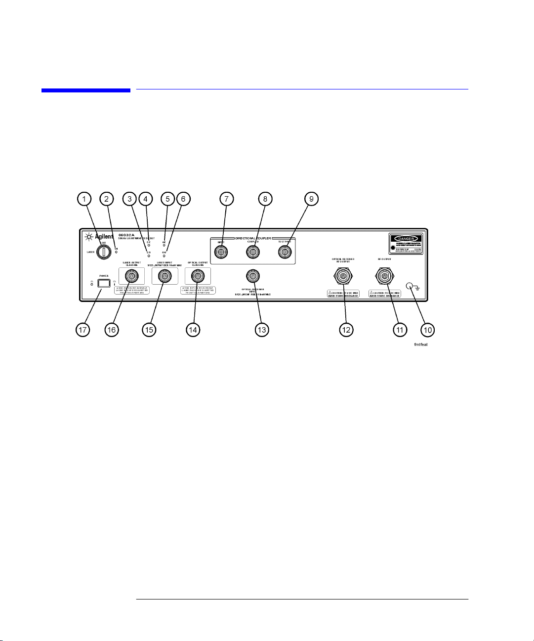
Front Panel Features

Figure 1-1. 86032A Front Panel

1-8

Getting Started

Front Panel Features

1. LASER Key Turns the laser on and off. Note that the laser is not operational until it is activated by the 86030A software program. You can turn on the laser manually from the Diagnostic software. From the Windows Start menu, select Programs, Agilent Technologies 50 GHz LCA, 50 GHz Diagnostics. From the Laser menu, click Laser ON. Make sure the laser key on the 86032A is in the on position.

WARNING Do NOT, under any circumstances, look into the optical output or any

fiber/device attached to the output while the laser is in operation.

Refer to “Laser Safety Considerations” on page 1-30.

2. Laser LED Indicates the state of the laser. When the LED is lit, the laser is on. Note that the laser is not operational until it is activated by the 86030A software program. You can turn on the laser manually from the Diagnostic software. From the Windows Start menu, select Programs, Agilent Technologies 50 GHz LCA, 50 GHz Diagnostics. From the Laser menu, click Laser ON.

3. E/O LED When on, indicates the internal measurement path is selected for an E/O (electrical-to-optical) device.

4. E/E LED When on, the internal measurement path is selected for an E/E (electrical-to-electrical) device. The test set is in a bypass mode for E/E device selection and the laser is shut down. The test set will need to be in the ON position for use in E/E mode.

5. O/E LED When on, the internal measurement path is selected for an (optical-to-electrical) O/E device.

6. O/O LED When on, the internal measurement path is selected for an (optical-to-optical) O/O device.

7. DIRECTIONAL COUPLER

INPUT

8. DIRECTIONAL COUPLER

COUPLED

9. DIRECTIONAL COUPLER

TEST PORT

10. Grounding Receptacle Ground path that is provided to connect a static strap.

11. RF OUTPUT RF output that provides RF drive power for E/O devices.

12. OPTICAL RECEIVER RF

OUTPUT

Input for the optical direction coupler. This port is usually connected to the OPTICAL OUTPUT.

Port for the coupler output. This port is usually connected to the OPTICAL RECEIVER INPUT.

Coupler output port (transmission) or test port (reflection).

Test set optical receiver output

1-9

Getting Started

Front Panel Features

13.OPTICAL RECEIVER INPUT

14. OPTICAL OUTPUT Modulator output.

15. LASER INPUT External laser input

16. LASER OUTPUT Output of internal laser

17. POWER Switch Turns the instrument power on.

Test set optical receiver input

CAUTION Use care in handling optical connectors. Damage to an optical test port

connector can require a costly repair and lost productivity for the system. Keep optical cables connected to the test ports to protect the connectors from damage. Also, make sure to clean the connectors before each use. Refer to

“Accurate Measurements” on page 1-33.

1-10

Rear Panel Features

Getting Started

Rear Panel Features

Figure 1-2. 86032A Rear Panel

1. Remote Programming

Connector

2. Laser Remote Shutdown Turns the laser on or off. When the BNC short is connected, the

3. Line Module This assembly houses the line cord connector.

4. RF REF OUTPUT RF output of the test set that is used to route the 8517B electrical

5. EXT ALC DC output from the levelling detector on the internal ALC circuit.

6. RF INPUT RF input port from the source output of the network analyzer.

Allows for remote control of the instrument’s front panel via the 86030A software installed on the system PC.

laser is enabled. When removed, the laser is disabled.

test set for phase locking.

This output is routed to the EXT ALC port of the network analyzer source.

1-11

Getting Started

Software Overview

The 86030A software sets up instrument states on the network analyzer and lightwave test set, and guides you through the measurement calibration and measurement procedures. The program combines the measurement calibration traces with the calibration data response of the lightwave receiver, and loads the result back into the network analyzer to provide calibrated lightwave measurements. You can save and view trace data using Microsoft Excel, and manually control the 86032A test set operation.

1-12

Getting Started

File Menu

The File menu is used to save data as either an ASCII text file or an Excel worksheet. Using Graph Excel Data allows you to automatically view saved data in an Excel worksheet as tabular data, or as graphical data in log magnitude, phase or delay formats. The File menu is also used to exit the application.

Save Data

Text File Text File allows you to save data as an ASCII text file in four different formats:

Raw Data, Log Magnitude, Phase, or Delay.

1-13

Getting Started

File Menu

Raw Data saves trace data in a ASCII text format (.txt) known as a CITIFile (common instrumentation transfer and interchange file). The CITIFile format is useful when data will be exchanged with another network analyzer. The data file saves both real and imaginary pairs independent of the format of the active screen. However, any trace smoothing that was applied to the measurement will not be saved (that is, Smoothing On is activated from the 8510C Response menu).

Formatted Data, Log Mag, Phase, Delay saves trace data with any trace smoothing that was applied to the measurement (that is, Smoothing On is activated from the 8510C Response menu), but only retains the values of the format that was selected for saving (that is, Log Magnitude, Phase, or Delay).

Excel File Excel File allows you to save the trace display as a Microsoft Excel workbook

(.xls extension). The Excel format is useful when you want to view or edit the data in an Excel spreadsheet.

Raw Data saves both real and imaginary pairs independent of the format of the active screen. This data can later be viewed in either Log Magnitude or Phase format from the File, Graph Excel Data menu. Any trace smoothing that was applied to the measurement will not be saved (that is, if Smoothing On is activated from the 8510C Response menu).

Formatted Data saves trace data and any trace smoothing that was applied to the measurement, but only viewed using the format that the data was originally saved (that is, Log Magnitude, Phase, or Delay).

1-14

Getting Started

File Menu

Log Mag saves the log magnitude format. This is the standard Cartesian format used to display magnitude-only measurements of insertion loss, return loss, or absolute power in dB versus frequency.

Phase saves the phase of data versus frequency in a Cartesian format. Delay saves the group delay format, with marker values given in seconds.

Group delay is the measurement of signal transmission time through a test device. It is defined as the derivative of the phase characteristic with respect to frequency. Since the derivative is basically the instantaneous slope (or rate of change of phase with frequency), a perfectly linear phase shift results in a constant slope, and therefore a constant group delay.

Graph Excel Data

Raw Data Data allows you to view trace data in either Log Magnitude or Phase format.

However, any trace smoothing that was applied to the measurement will not be captured. (that is, if Smoothing On was activated from the 8510C Response menu).

Log Magnitude displays the trace data in Cartesian format as logarithmic (dB) magnitude versus frequency.

Phase displays the trace data in Cartesian format as phase versus frequency.

Formatted Data, Formatted Data allows you to view trace data in the format that it was saved

(that is, Log Magnitude, Phase, or Delay) including any trace smoothing that was applied to the measurement

1-15

Getting Started

File Menu

Log Mag displays the log magnitude format. This is the standard Cartesian format used to display magnitude-only measurements of insertion loss, return loss, or absolute power in dB versus frequency.

Phase displays the phase shift of data versus frequency in a Cartesian format. Delay displays the group delay format, with marker values given in seconds.

Figure 1-3.

Note, however, that the phase characteristic typically consists of both linear and higher order (deviations from linear) components. The linear component can be attributed to the electrical length of the test device, and represents the average signal transit time. The higher order components are interpreted as variations in transit time for different frequencies, and represent a source of signal distortion. See Figure 1-4.

1-16

Figure 1-4.

Getting Started

File Menu

Group Delay τ

Gφ



Gω

in Radians in Radians

1



360°

Gφ

⋅

φ in Degrees

I in Hz (ω 2πI )

The analyzer computes group delay from the phase slope. Phase data is used to find the phase change, ∆φ, over a specified frequency aperture, ∆ƒ, to obtain an approximation for the rate of change of phase with frequency (Fig-

ure 1-5). This value, τ

, represents the group delay in seconds assuming linear

phase change over ∆ƒ. It is important that ∆φ be ≤180°, or errors will result in the group delay data. These errors can be significant for long delay devices.

Figure 1-5.

When deviations from linear phase are present, changing the frequency step can result in different values for group delay. Note that in this case the computed slope varies as the aperture ∆ƒ is increased (Figure 1-6). A wider aper-

1-17

Getting Started

File Menu

ture results in loss of the fine grain variations in group delay. This loss of detail is the reason that in any comparison of group delay data it is important to know the aperture used to make the measurement.

Figure 1-6.

In determining the group delay aperture, there is a trade-off between resolution of fine detail and the effects of noise. Noise can be reduced by increasing the aperture, but this will tend to smooth out the find detail. More detail will become visible as the aperture is decreased, but the noise will also increase, possibly to the point of obscuring the detail. A good practice is to use a smaller aperture to assure that small variations are not missed, then increase the aperture to smooth the trace.

1-18

Exit

Exit closes the 86030A software application.

Getting Started

File Menu

1-19

Getting Started

Options Menu

The Options menu allows you to set and monitor system functions.

Auto Bias

Auto Bias allows you bias the modulator to operate at quadrature or at maximum optical power. Under typical circumstances the lightwave modulator is biased to operate at quadrature. Quadrature is the point where the slope of the optical power versus voltage is maximally positive. Refer to Figure .

1-20

Getting Started

Options Menu

Power at Quadrature (1)

Voltage at Quadrature (2)

Figure 1-7. Effect of Bias Voltage on Modulated Optical Power

The power where the optical power versus bias voltage slope is maximum for a positive slope.

The voltage where the optical power versus bias voltage slope is maximum for a positive slope.

1-21

Getting Started

Options Menu

Voltage at Maximum Optical Power (3)

Voltage at Minimum Optical Power (4)

Maximum Optical Power (5)

Minimum Optical Power (6)

The voltage at which the maximum output power occurs (V

The voltage at which the minimum output power occurs (V

min

max

The maximum output power.

The minimum output power.

How to Determine if Auto Bias Values are Reasonable

The following formulas will help you to determine if the modulator auto bias settings are valid. Refer to Figure .

Voltage at Maximum Optical Power – Voltage at Minimum Optical Power should between 3 and 6 volts.

Voltage at Quadrature should be approximately

Maximum Optical Power should be > 3 dBm Power at Quadrature should be > 0dBm Tip: You can set the this value manually. From the Tools menu, click on Moni-

tor Test Set. In the Modify Bias Voltage text box, enter the desired value and then click Set Modulator Bias Voltage to.

Refer to “Modulator Troubleshooting Tips” on page 6-16 for more information.

9PD[ 9PLQ 

1-22

Getting Started

Options Menu

Auto Bias At Cal

Auto Bias At Cal when selected, an auto bias is performed before each calibration. The auto bias is performed after you click either Resp Cal or Resp-Isol Cal.

Customize

Customize allows you to set and monitor certain parameters that affect the operation of the system.

Standard The Standard Settings dialog box allows you to set and monitor certain param-

eters controlled by the network analyzer.

1-23

Getting Started

Options Menu

GPIB Address displays the current address setting for the analyzer. This value must correspond to the actual address on the 8510 GPIB address bus. Failure of these two numbers to match will prevent operation.

Average Factor is used to improve the sensitivity of the measurement. For the Step Mode of operation for each modulation frequency point, multiple data point samples (equal to the number of averages) are measured by the system, and averaged together to provide a single average value. Averaging multiple data points together reduces the effects of noise on the measurement. The improvement in sensitivity is equal to:

log number of averages

Note the 8510C network analyzer only averages with powers of 2 (that is, 1, 2, 4, 8, 16, 32, 64, 128, 256, 512, 1024, and so on). Therefore, if an averaging factor of 500 is set on the analyzer, the analyzer will default to 256 averages.

Bias Interval, mins corresponds to the number of minutes before prompting you to perform another modulator auto bias.

Refl Standard% corresponds to the percent of reflection of the Reflection Standard used in the system. This is useful for O/O reflection modes.

Averaging when selected, the network analyzer will perform averaging at each data point.

Split Screen E/O when selected, the network analyzer displays both the bandwidth and reflection measurement on the display. This function is only valid with an E/O Bandwidth and Reflection measurement. Bandwidth is displayed on channel 1 and Reflection is displayed on channel 2. When this function is cleared, use the network analyzer front panel channel buttons to select between the two measurements.

1-24

Getting Started

Options Menu

Time Date Stamp when selected, the time and date stamp is applied to the trace on the network analyzer.

Scale Excel Chart when selected, the trace data saved from the network analyzer will be auto-scaled to fit into an Excel chart.

Step Sweep/Ramp Sweep toggles between step sweep and ramp sweep modes.

Step Sweep is a digital sweep beginning at the start frequency and ending at the stop frequency with the source phase locked and the data measured at a frequency interval determined by the number of points selected on the network analyzer (STIMULUS MENU, STEP). An up arrow on the trace identifies the data point just measured. The ramp mode is recommended when you need the best modulation frequency accuracy and repeatability.

Dwell time prior to measurement at each frequency point is controlled by the sweep time setting. Measurement time at each point is determined by the averaging factor.

NOTE System specifications are only warranted when using the Step Sweep mode of

operation.

Ramp Sweep selects continuous linear analog sweeps beginning at the start frequency and ending at the stop frequency. The rate is determined by the sweep time, measuring data at frequency intervals set by the number of points. (8510 access, STIMULUS MENU, RAMP)

Advanced The Advanced Settings dialog box allows changing of default power values.

1-25

Getting Started

Options Menu

External Leveling when checked, the system uses external leveling. When cleared, the system uses internal leveling. Normal system operation uses external leveling.

Src Pwr, E to X, dBV for E/O mode and E/ E mode, displays the 83651A external leveling source power.

Src Pwr, O to X, dBV for O/E mode and O/O mode, displays the 83651A external leveling source power.

Default Settings when selected, resets the source power to its factory default values.

System Verification

A System Verification performs a measurement on the verification device over the entire frequency range. The verification device is the 83440D lightwave detector supplied in the system verification kit. Once the verification is completed, the results are displayed in an Excel worksheet along with the error bars that were computed from the factory measurement of the verification device. For the system verification to pass, the verification device trace must fit within the error bars. A pass or fail indicator is displayed at the bottom of the worksheet. Refer to “Lightwave Verification” on page 5-3 for more inforation.

1-26

Getting Started

Tools Menu

The Tools menu is used to monitor and modify 86032A test set parameters.

Modify Test Set

Curent Laser Output Power (dBm) displays the value of the laser power coming from the LASER OUTPUT port of the test set.

Set Laser Output Power to:(dBm), when Modify Power is selected, the value will be updated to the value specified in this text box.

1-27

Getting Started

Tools Menu

Modify Power sets the internal laser of the 86030A test set to the power specified in the Modify Power text box. This value will be used until you restart the 86030A software. Valid settings are from 0 dBm to 10 dBm.

Set Optical Output Pwr to Nominal Setting sets the laser to its factory default setting. When the software is started, the power always defaults back to the factory setting.

Current Modulator Bias Voltage (V) displays the value last applied to the internal modulator bias tee attached to the optical modulator.

Set Modulator Bias Voltage to: (V), when Modify Bias Voltage is selected, the bias voltage will be updated to the value specified in this text box. The range is –10 to +10 volts.

Modify Bias Voltage sets the bias voltage to the value entered in the Set Modulator Bias Voltage text box.

Turn Laser On turns on the laser inside the 86032A test set. This command does not change the power of the laser. This function is useful in E/O mode when you may want to use the internal high power laser as a stimulus for testing optical modulators. The optical power is normally off in the E/O mode.

Turn Laser Off turns off the laser inside the 86032A test set. This command does not change power of the laser. If the laser is turned off and then turned back on again, the original power of the laser will be used.

Set Mod. Bias to Quadrature when clicked, performs an auto bias on the modulator and sets the modulator bias voltage to the midpoint of the average optical power curve and the peak of the modulated optical power curve. Biasing at quadrature maximizes the modulation response and minimizes distortion of the modulated signal.

The power of the laser is assumed to have been previously set. If the laser power is too low or if the laser is turned off, the auto bias routine will fail and display a message indicating that a bias point could not be found. For this command to function properly, the laser power should left at its default setting or set to a reasonable power value (between 3 and 10 dBm) prior to performing this function.

Set Mod Bias to Maximum when selected, performs an auto bias on the modulator and sets the modulator at maximum optical output power.

The power of the laser is assumed to have been previously set. If the laser power is too low or if the laser is turned off, the auto bias routine will fail and display a message indicating that a bias point could not be found. For this command to function properly, the laser power should be left to its default setting or set to a reasonable power value (between 3 and 10 dBm) prior to performing this function.

1-28

Getting Started

Tools Menu

E/X when selected, puts the 86032A test set into electrical excitation mode. The RF signal coming into the test set will be routed out of the front panel marked “RF OUTPUT.” Therefore, the RF signal will not be routed to the optical modulator in the test set.

O/X when selected, puts the 86032A test set into optical excitation mode. The RF signal coming into the test set will be routed to the optical modulator.

Monitor Test Set

The Monitor Test Set dialog box is used to monitor and update the power and voltage levels of the 86032A test set.

Optical Output Power (dBm) displays the current optical power coming from the 86032A OPTICAL OUTPUT port.

Optical Receiver Input (dBm) displays the current optical power coming into the 86032A OPTICAL RECEIVER INPUT port.

Current Modulator Bias Setting (V) displays the current value of the 86032A bias voltage on the modulator.

1-29

Getting Started

Laser Safety Considerations

Laser Safety Laser radiation in the ultraviolet and far infrared parts of the spectrum can

cause damage primarily to the cornea and lens of the eye. Laser radiation in the visible and near infrared regions of the spectrum can cause damage to the retina of the eye.

The CW laser sources use a laser from which the greatest dangers to exposure are:

1 To the eyes, where aqueous flare, cataract formation, and/or corneal burn are

possible.

2 To the skin, where burning is possible.

WARNING Do NOT, under any circumstances, look into the optical output or any

fiber/device attached to the output while the laser is in operation.

This system should be serviced only by authorized personnel. Do not enable the laser unless fiber or an equivalent device is attached to the

optical output connector.

CAUTION Use of controls or adjustments or performance of procedures other than those

specified herein can result in hazardous radiation exposure.

Laser Classifications

United States-FDA Laser Class IIIb. The system is rated USFDA (United States Food and Drug Administration) Laser Class IIIb according to Part 1040, Performance Standards for Light Emitting Products, from the Center for Devices and Rad iological Health.

International-IEC Laser Class 3B. The system is rated IEC (International Electrotechnical Commission) Laser Class 3B laser products according to Publication 825.

International-IEC 825. The system helps satisfy the International (IEC825) safety requirements with the use of a REMOTE SHUTDOWN and a KEY SWITCH.

1-30

Getting Started

Laser Safety Considerations

Laser Warning Labels

The 86030A is shipped with the following warning labels. For systems used outside of the USA, both laser aperture and laser warning labels will be included with the shipment (The labels are located in the same box as this manual). Place these labels directly over the USA laser warning and aperture labels.

Figure 1-8. Laser safety label locations

Electrical Safety The electrical safety considerations are documented in the section “General

Safety Considerations” on page -iv. Familiarize yourself with the safety mark-

ings and instructions before operating this system.

Service Limited service may be performed on this system in accordance with informa-

tion provided in Chapter 6, “Maintenance”. For all other repairs the system must be returned to Agilent Technologies.

Maintenance On a daily basis, practice the techniques for proper connector use and care.

Refer to the Lightwave Connection Techniques for Better Measurements booklet. If you should ever need to clean the cabinet, use a damp cloth only.

CAUTION Exposure to temperatures above 55°C may cause the front panel fiber to

retract. In this case a matching compound can be used to temporarily improve return loss. However, the system should be returned to Agilent Technologies for repair.

CAUTION This product is designed for use in INSTALLATION CATEGORY II and

POLLUTION DEGREE 2, per IEC 1010 and 664 respectively.

1-31

Getting Started

Laser Safety Considerations

Learn proper connector care

When you use improper cleaning and handling techniques, you risk expensive system repairs, damaged cables, and compromised measurements. Repair of damaged connectors due to improper use is not covered under warranty.

Clean all cables before applying to any connector. Refer to the Lightwave Connections Techniques for Better Measurements booklet.

1-32

Getting Started

Accurate Measurements

Today, advances in measurement capabilities make connectors and connection techniques more important than ever. Damage to the connectors on calibration and verification devices, test ports, cables, and other devices can degrade measurement accuracy and damage instruments. Replacing a damaged connector can cost thousands of dollars, not to mention lost time! This expense can be avoided by observing the simple precautions presented in this book. This book also contains a brief list of tips for caring for electrical connectors.

Choosing the Right Connector

A critical but often overlooked factor in making a good lightwave measurement is the selection of the fiber-optic connector. The differences in connector types are mainly in the mechanical assembly that holds the ferrule in position against another identical ferrule. Connectors also vary in the polish, curve, and concentricity of the core within the cladding. Mating one style of cable to another requires an adapter. Agilent Technologies offers adapters for most instruments to allow testing with many different cables. The Figure 1-9

on page 1-34 shows the basic components of a typical connectors.

The system tolerance for reflection and insertion loss must be known when selecting a connector from the wide variety of currently available connectors. Some items to consider when selecting a connector are:

• How much insertion loss can be allowed?

• Will the connector need to make multiple connections? Some connectors are

better than others, and some are very poor for making repeated connections.

• What is the reflection tolerance? Can the system take reflection degradation?

• Is an instrument-grade connector with a precision core alignment required?

• Is repeatability tolerance for reflection and loss important? Do your specifica-

1-33

Getting Started

Accurate Measurements

tions take repeatability uncertainty into account?

• Will a connector degrade the return loss too much, or will a fusion splice be required? For example, many DFB lasers cannot operate with reflections from connectors. Often as much as 90 dB isolation is needed.

Figure 1-9. Basic components of a connector.

Over the last few years, the FC/PC style connector has emerged as the most popular connector for fiber-optic applications. While not the highest performing connector, it represents a good compromise between performance, reliability, and cost. If properly maintained and cleaned, this connector can withstand many repeated connections.

However, many instrument specifications require tighter tolerances than most connectors, including the FC/PC style, can deliver. These instruments cannot tolerate connectors with the large non-concentricities of the fiber common with ceramic style ferrules. When tighter alignment is required, Agilent instruments typically use a connector such as the Diamond HMS-10, which has concentric tolerances within a few tenths of a micron. Agilent then uses a special universal adapter, which allows other cable types to mate with this precision connector. See Figure 1-10 on page 1-35.

1-34

Getting Started

Accurate Measurements

Figure 1-10. Universal adapters

The HMS-10 encases the fiber within a soft nickel silver (Cu/Ni/Zn) center which is surrounded by a tough tungsten carbide casing, as shown in Figure

1-11.

Figure 1-11. Cross-section of the Diamond HMS-10 connector.

The nickel silver allows an active centering process that permits the glass fiber to be moved to the desired position. This process first stakes the soft nickel silver to fix the fiber in a near-center location, then uses a post-active staking to shift the fiber into the desired position within 0.2 µm. This process, plus the keyed axis, allows very precise core-to-core alignments. This connector is found on most Agilent lightwave instruments.

1-35

Getting Started

Accurate Measurements

The soft core, while allowing precise centering, is also the chief liability of the connector. The soft material is easily damaged. Care must be taken to minimize excessive scratching and wear. While minor wear is not a problem if the glass face is not affected, scratches or grit can cause the glass fiber to move out of alignment. Also, if unkeyed connectors are used, the nickel silver can be pushed onto the glass surface. Scratches, fiber movement, or glass contamination will cause loss of signal and increased reflections, resulting in poor return loss.

Inspecting Connectors

Because fiber-optic connectors are susceptible to damage that is not immediately obvious to the naked eye, bad measurements can be made without the user even being aware of a connector problem. Although microscopic examination and return loss measurements are the best way to ensure good connections, they are not always practical. An awareness of potential problems, along with good cleaning practices, can ensure that optimum connector performance is maintained. With glass-to-glass interfaces, it is clear that any degradation of a ferrule or the end of the fiber, any stray particles, or finger oil can have a significant effect on connector performance.

Figure 1-12 shows the end of a clean fiber-optic cable. The dark circle in the

center of the micrograph is the fiber’s 125 µm core and cladding which carries the light. The surrounding area is the soft nickel-silver ferrule. Figure 1-13 shows a dirty fiber end from neglect or perhaps improper cleaning. Material is smeared and ground into the end of the fiber causing light scattering and poor reflection. Not only is the precision polish lost, but this action can grind off the glass face and destroy the connector.

Figure 1-14 shows physical damage to the glass fiber end caused by either

repeated connections made without removing loose particles or using improper cleaning tools. When severe, the damage on one connector end can be transferred to another good connector that comes in contact with it.

The cure for these problems is disciplined connector care as described in the following list and in “Cleaning Connectors” on page 1-40.

Use the following guidelines to achieve the best possible performance when making measurements on a fiber-optic system:

• Never use metal or sharp objects to clean a connector and never scrape the connector.

• Avoid matching gel and oils.

1-36

Figure 1-12. Clean, problem-free fiber end and ferrule.

Getting Started

Accurate Measurements

Figure 1-13. Dirty fiber end and ferrule from poor cleaning.

Figure 1-14. Damage from improper cleaning.

While these often work well on first insertion, they are great dirt magnets. The oil or gel grabs and holds grit that is then ground into the end of the fiber. Also, some early gels were designed for use with the FC, non-contacting con-

1-37

Getting Started

Accurate Measurements

nectors, using small glass spheres. When used with contacting connectors, these glass balls can scratch and pit the fiber. If an index matching gel or oil must be used, apply it to a freshly cleaned connector, make the measurement, and then immediately clean it off. Never use a gel for longer-term connections and never use it to improve a damaged connector. The gel can mask the extent of damage and continued use of a damaged fiber can transfer damage to the instrument.

• When inserting a fiber-optic cable into a connector, gently insert it in as straight a line as possible. Tipping and inserting at an angle can scrape material off the inside of the connector or even break the inside sleeve of connectors made with ceramic material.

• When inserting a fiber-optic connector into a connector, make sure that the fiber end does not touch the outside of the mating connector or adapter.

• Avoid over tightening connections. Unlike common electrical connections, tighter is not better. The purpose of

the connector is to bring two fiber ends together. Once they touch, tightening only causes a greater force to be applied to the delicate fibers. With connectors that have a convex fiber end, the end can be pushed off-axis resulting in misalignment and excessive return loss. Many measurements are actually improved by backing off the connector pressure. Also, if a piece of grit does happen to get by the cleaning procedure, the tighter connection is more likely to damage the glass. Tighten the connectors just until the two fibers touch.

• Keep connectors covered when not in use.

• Use fusion splices on the more permanent critical nodes. Choose the best con-

nector possible. Replace connecting cables regularly. Frequently measure the return loss of the connector to check for degradation, and clean every connector, every time.

All connectors should be treated like the high-quality lens of a good camera. The weak link in instrument and system reliability is often the inappropriate use and care of the connector. Because current connectors are so easy to use, there tends to be reduced vigilance in connector care and cleaning. It takes only one missed cleaning for a piece of grit to permanently damage the glass and ruin the connector.

Measuring insertion loss and return loss

Consistent measurements with your lightwave equipment are a good indication that you have good connections. Since return loss and insertion loss are key factors in determining optical connector performance they can be used to determine connector degradation. A smooth, polished fiber end should pro-

1-38

Getting Started

Accurate Measurements

duce a good return-loss measurement. The quality of the polish establishes the difference between the “PC” (physical contact) and the “Super PC” connectors. Most connectors today are physical contact which make glass-to-glass connections, therefore it is critical that the area around the glass core be clean and free of scratches. Although the major area of a connector, excluding the glass, may show scratches and wear, if the glass has maintained its polished smoothness, the connector can still provide a good low level return loss connection.

If you test your cables and accessories for insertion loss and return loss upon receipt, and retain the measured data for comparison, you will be able to tell in the future if any degradation has occurred. Typical values are less than 0.5 dB of loss, and sometimes as little as 0.1 dB of loss with high performance connectors. Return loss is a measure of reflection: the less reflection the better (the larger the return loss, the smaller the reflection). The best physically contacting connectors have return losses better than 50 dB, although 30 to 40 dB is more common.

To Te st Ins er t i on L os s

Use an appropriate lightwave source and a compatible lightwave receiver to test insertion loss. Examples of test equipment configurations include the following equipment:

• 71450A or 71451A Optical Spectrum Analyzers with Option 002 built-in white light source.

• 8702 or 8703 Lightwave Component Analyzer system.

• 83420 Chromatic Dispersion Test Set with an 8510 Network Analyzer.

• 8153 Lightwave Multimeter with a source and power sensor module.

To Te st Re t ur n L o s s

Use an appropriate lightwave source, lightwave receiver, and lightwave coupler to test return loss. Examples of test equipment configurations include the following equipment:

• Agilent 8703 Lightwave Component Analyzer.

• Agilent 8702 Lightwave Component Analyzer with the appropriate source,

receiver, and lightwave coupler.

• Agilent 8504 Precision Reflectometer.

• Agilent 8153 Lightwave Multimeter with a source and power sensor module in

conjunction with a lightwave coupler.

• Agilent 81554SM Dual Source and Agilent 81534A Return Loss Module.

1-39

Getting Started

Accurate Measurements

Visual inspection of fib er ends

Visual inspection of fiber ends can be helpful. Contamination or imperfections on the cable end face can be detected as well as cracks or chips in the fiber itself. Use a microscope (100X to 200X magnification) to inspect the entire end face for contamination, raised metal, or dents in the metal as well as any other imperfections. Inspect the fiber for cracks and chips. Visible imperfections not touching the fiber core may not affect performance (unless the imperfections keep the fibers from contacting).

Cleaning Connectors

The procedures in this section provide the proper steps for cleaning fiberoptic cables and Agilent universal adapters. The initial cleaning, using the alcohol as a solvent, gently removes any grit and oil. If a caked-on layer of material is still present, (this can happen if the beryllium-copper sides of the ferrule retainer get scraped and deposited on the end of the fiber during insertion of the cable), a second cleaning should be performed. It is not uncommon for a cable or connector to require more than one cleaning.

CAUTION Agilent strongly recommends that index matching compounds not be applied

to their instruments and accessories. Some compounds, such as gels, may be difficult to remove and can contain damaging particulates. If you think the use of such compounds is necessary, refer to the compound manufacturer for information on application and cleaning procedures.

Table 1-3. Cleaning Accessories

Item Agilent Part Number

Isopropyl alcohol 8500-5344

Cotton swabs 8520-0023

Small foam swabs 9300-1223

Compressed dust remover (non-residue) 8500-5262

1-40

Getting Started

Accurate Measurements

Table 1-4. Dust Caps Provided with Lightwave Instruments

Item Agilent Part Number

Laser shutter cap 08145-64521

FC/PC dust cap 08154-44102

Biconic dust cap 08154-44105

DIN dust cap 5040-9364

HMS10/Agilent dust cap 5040-9361

ST dust cap 5040-9366

To clean a non-lensed connector

CAUTION Do not use any type of foam swab to clean optical fiber ends. Foam swabs can

leave filmy deposits on fiber ends that can degrade performance.

1 Apply pure isopropyl alcohol to a clean lint-free cotton swab or lens paper.

Cotton swabs can be used as long as no cotton fibers remain on the fiber end after cleaning.

2 Clean the ferrules and other parts of the connector while avoiding the end of

the fiber.

3 Apply isopropyl alcohol to a new clean lint-free cotton swab or lens paper. 4 Clean the fiber end with the swab or lens paper.

Do not scrub during this initial cleaning because grit can be caught in the swab and become a gouging element.

5 Immediately dry the fiber end with a clean, dry, lint-free cotton swab or lens

paper.

6 Blow across the connector end face from a distance of 6 to 8 inches using

filtered, dry, compressed air. Aim the compressed air at a shallow angle to the fiber end face.

Nitrogen gas or compressed dust remover can also be used.

CAUTION Do not shake, tip, or invert compressed air canisters, because this releases

particles in the can into the air. Refer to instructions provided on the compressed air canister.

1-41

Getting Started

Accurate Measurements

Caring for Electrical Connections

The following list includes the basic principles of microwave connector care. For more information on microwave connectors and connector care, consult the Connector Care Manual, part number 08510-90064.

Handling and Storage

• Keep connectors clean

• Extend sleeve or connector nut

• Use plastic endcaps during storage

• Do not touch mating plane surfaces

• Do not set connectors contact-end down

Visual Inspection

• Inspect all connectors carefully before every connection

• Look for metal particles, scratches, and dents

• Do not use damaged connectors

Cleaning

• Try cleaning with compressed air first

• Clean the connector threads

• Do not use abrasives

• Do not get liquid onto the plastic support beads

Making Connections

• Align connectors carefully

• Make preliminary connection lightly

• To tighten, turn connector nut only

• Do not apply bending force to connection

• Do not overtighten preliminary connection

• Do not twist or screw in connectors

• Do not tighten past the “break” point of the torque wrench

1-42

Getting Started

Electrostatic Discharge Information

Electrostatic discharge (ESD) can damage or destroy electronic components. All work on electronic assemblies should be performed at a static-safe work station. The following figure shows an example of a static-safe work station using two types of ESD protection:

• Conductive table-mat and wrist-strap combination.

NOTE For the 86030A 50 GHz LCA system, the static strap is attached to the 86032A

front panel grounding receptacle. Refer to “Front Panel Features” on page 1-8.

• Conductive floor-mat and heel-strap combination.

1-43

Getting Started

Electrostatic Discharge Information

Both types, when used together, provide a significant level of ESD protection. Of the two, only the table-mat and wrist-strap combination provides adequate ESD protection when used alone.

To ensure user safety, the static-safe accessories must provide at least 1 MΩ of isolation from ground. Refer to Table 15 on page 1-45 for information on ordering static-safe accessories.

WARNING These techniques for a static-safe work station should not be used

when working on circuitry with a voltage potential greater than 500 volts.

1-44

Getting Started

Electrostatic Discharge Information

Reducing ESD Damage

The following suggestions may help reduce ESD damage that occurs during testing and servicing operations.

• Personnel should be grounded with a resistor-isolated wrist strap before removing any assembly from the unit.

• Be sure all instruments are properly earth-grounded to prevent a buildup of static charge.

Table 15. Static-Safe Accessories

Agilent Part Number

9300-0797

9300-0980 Wrist-strap cord 1.5 m (5 ft.)

9300-1383 Wrist-strap, color black, stainless steel, without cord, has four adjustable

9300-1169 ESD heel-strap (reusable 6 to 12 months).

Description

Set includes: 3M static control mat 0.6 m ft.) ground wire. (The wrist-strap and wrist-strap cord are not included. They must be ordered separately.)

links and a 7 mm post-type connection.

× 1.2 m (2 ft.× 4 ft.) and 4.6 cm (15

1-45

Getting Started

Quick Start

This procedure steps you through the process of making your first measurement. The verification kit supplied with your system contains a photo detector, which we will use to make an optical-to electrical (O/E) bandwidth response measurement.

Photodiode responsivity (amps/watt) refers to how a change in optical power is converted to a change in output electrical current. As the frequency of modulation increases, eventually the receiver responsivity will rolloff. Thus, the device has a limited modulation bandwidth. The measurement of modulation bandwidth consists of stimulating the photodiode with a source of modulated light and measuring the output response current with an electrical receiver. The frequency of the modulation is swept to allow examination of the photodiode over a wide range of modulation frequencies.

1 From the Windows Start menu, select Programs, Agilent Technologies 50 GHz

LCA, 50 GHz LCA Main to open the software.

1-46

2 Follow the instructions for the Laser power prompt, then press OK.

Getting Started

Quick Start

3 When the software is first opened, a modulator auto-bias will automatically be

performed, which takes approximately 2 minutes. The modulator is automatically biased to the optimum (quadrature) performance condition.

An auto-bias does not need to be performed before each individual measurement but should be performed for any of the following conditions:

• at least once every eight hours

• if the temperature has drifted more than 3°C from the user calibration tem-

perature

• if the jumper between the 86032A LASER OUTPUT and LASER INPUT has

been removed and replaced. This routine takes approximately two minutes and the results will be displayed on the screen. Refer to “Auto Bias” on page 1-20.

1-47

Getting Started

Quick Start

4 When the auto bias is finished, click OK to close the Modulator Auto Bias

window.

The system has finished setup procedures.

1-48

Getting Started

Quick Start

Making an Optical to Electrical Measurement

1 In the System Modes area, click on O/E (the default mode) to set up for an

optical to electrical measurement.

2 In the Measurement Types area, click on BandWidth. 3 In the Control Options area, click on the New User Cal. 4 The message, “Set 8510 to desired Start Frequency, Stop Frequency, and the

Number of Points” appears. To do this:

a On the 8510 analyzer under the STIMULUS area, set the Start frequency to

45 MHz and the Stop Frequency to 50 GHz.

b From the STIMULUS MENU, select NUMBER of POINTS, then 801. c From the RESPONSE MENU, select AVERAGING ON and set to 128 points.

5 Click OK in the application message box.

1-49

Getting Started

Quick Start

6 Follow the onscreen instructions to configure the test set for calibration, then

press OK.

7 In the Control Options area, click on Resp-Isol to perform a response plus

isolation calibration.

8 Follow the on-screen instructions for the Response portion of the calibration

procedure.

9 Follow the on-screen instructions for the Isolation portion of the calibration

procedure. The system first takes an uncorrected measurement of the internal O/E con-

verter in the 86032A test set. This raw data along with factory calibration data for the internal O/E are used to construct a calibration file for the system.

You can monitor the System Status area as the calibration is in progress. Once the calibration is completed, you can view the calibration results in the Calibration Information area.

You are now ready to make a bandwidth response measurement.

10 Follow the on-screen instructions for the measurement setup. 11 From the 8510 RESPONSE menu, adjust the scale to best fit the trace on the

screen.

a Select REF VALUE and use the knob to center the trace around the display line. b Select SCALE and decrease the dB/div to expand the trace across the display

(approximately 2 dB/div).

c Repeat steps a and b to get the best view.

12 Select the RESPONSE MENU key, then SMOOTHING ON. 13 Save the trace data to an Excel file by selecting File, Save Data, Excel File, then,

Form Log Mag.

14 In the Save to Excel dialog box, enter quick_start as the trace file name then click

OK.

You can now view the trace by selecting File, Graph Excel Data, Form Log Mag and then Open the Quick_Start file. Alternately, you can open a session of Excel and view or manipulate the trace file from there.

Or, you can further analyze the trace data by using the controls on the 8510C.

1-50

Getting Started

Quick Start

1-51

Getting Started

Quick Start

1-52

“The Calibrations” on page 2-2 “O/O Response and Isolation Bandwidth Calibration” on page 2-5 “O/E Response and Isolation Bandwidth Calibration” on page 2-8 “O/E Response and Match Bandwidth Calibration” on page 2-11 “E/O Response and Isolation Bandwidth Calibration” on page 2-20 “Electrical Mismatch Ripple and its Effects on Measurements.” on page 2-25 “Magnitude Response and Deviation From Linear Phase of a Lightwave Receiver” on page 2-37 “O/E RF Overload Detection Measurement” on page 2-47

Measurement Techniques

The Calibrations

The 86030A software can perform many different types of calibrations depending on your device type and measurement needs. Following is a list of all of the available calibrations.

• O/O

• Bandwidth Measurement Response Response/Isolation

• Reflection Measurement Response Response/Isolation

• O/E

• Bandwidth Response Response/Isolation Response/Match

• Reflection Response Response/Isolation

• Bandwidth & Reflection Response Response/Isolation

• E/O

• Bandwidth Response Response/Isolation

• Reflection Response

• Bandwidth & Reflection Response Response/Isolation

• Reflection Sensitivity Response

• E/E

Use the 8510C for electrical calibrations and measurements.

2-2

Table 2-1. Purpose and Use of Different Calibration Procedures

Measurement Techniques

The Calibrations

Calibration Procedure

Response Transmission or reflection measurement

Response & Isolation

S11 1-port Reflection of any one-port device or well

S22 1-port Reflection of any one-port device or well

Full 2-port Transmission or reflection of highest

Response Transmission or reflection measurement

Corresponding Measurement Errors Removed Standard Procedure

Electrical

when the highest accuracy is not required.

Transmission of high insertion loss devices or reflection of high return loss devices. Not as accurate as 1-port or 2-port calibration.

terminated two-port device.

accuracy for two-port devices.

Optical (O, O/O)

when the highest accuracy is not required.

Frequency response Thru for transmission,

open or short for reflection

Frequency response plus isolation in transmission or directivity in reflection.

Directivity, source match, frequency response

Directivity, source match, load match, isolation, frequency response, each in forward and reverse directions.

Frequency response Optical thru for

Same as response plus isolation std (load)

Short, open, and load(s)

Short, open, and load(s). Two loads needed for isolation.

transmission, Fresnel or Reflector for reflection

Response & Isolation

Response Transmission measurement Frequency response Optical and/or electrical

Response & Isolation

Transmission of high insertion loss devices or reflection of high return loss devices.

Optical (O/E)

Transmission of high Insertion loss devices Frequency response plus

Frequency response, plus isolation in transmission or directivity in reflection.

isolation

Same as response plus disconnect cable or turn off laser.

thrus Same as Response plus

disconnect cable or turn off laser.

2-3

Measurement Techniques

The Calibrations

Table 2-1. Purpose and Use of Different Calibration Procedures

Calibration Procedure

Response & Match

Corresponding Measurement Errors Removed Standard Procedure

Transmission measurement for devices with large electrical reflectivity.

Optical (E/O)

Response Transmission or reflection sensitivity

measurement.

Response and

Transmission of high insertion loss devices. Frequency response plus

Isolation

Note: If cables, connectors, or adapters are removed fro the measurement setup that

were used in the calibration, their effect must be accounted for by adding a port extension equivalent to the electrical length of the missing component(s).

Frequency response plus electrical mismatch

Same as Response plus short, opens, and loads.

Frequency response Optical and /or electrical

thrus for transmission, optical load for reflection sensitivity

Same as response plus

isolation

disconnect the cable or turn off the laser.

2-4

Measurement Techniques

O/O Response and Isolation Bandwidth Calibration

The following procedure shows you how to make a response and isolation bandwidth calibration.

1 In the System Modes area in the Setup Screen, click on O/O to setup for an

optical to electrical measurement.

2 In the Measurement Types area, click on BandWidth. 3 In the Control Options area, click on New User Cal. 4 The message, “Set 8510 to desired Start Frequency, Stop Frequency,

Averaging, and the Number of Points” appears. To do this: a On the 8510 analyzer under the STIMULUS area, set the Start frequency and

the Stop Frequency to the frequency range required for your measurement.

b From the STIMULUS MENU, select NUMBER of POINTS, then select the number

of data points, for example, 801 points.

c From the RESPONSE MENU, select AVERAGING ON/restart, then enter the

number of averages. For example, for 128 averages enter 128 x1.

5 In the Control Options area, click on Resp-Isol to perform a response plus

isolation calibration.

6 Follow the on-screen instructions to complete the calibration procedure.

2-5

Measurement Techniques

O/O Response and Isolation Bandwidth Calibration

2-6

Measurement Techniques

O/O Response and Isolation Bandwidth Calibration

The figure below shows the results of an optical to optical measurement of a through line with 0 dB loss. The magnitude of the trace (that is, the vertical axis) is measured in dBo. For more information, refer to “O/O Display Scaling

Calculations” on page 3-16.

Figure 2-1. Measurement results of a through line

2-7

Measurement Techniques

O/E Response and Isolation Bandwidth Calibration

The following procedure shows you how to make an Optical to Electrical response and isolation bandwidth calibration.

1 In the System Modes area in the Setup Screen, click on O/E to setup for an

optical to electrical measurement.

2 In the Measurement Types area, click on BandWidth. 3 In the Control Options area, click on New User Cal. 4 The message, “Set 8510 to desired Start Frequency, Stop Frequency,

Averaging, and the Number of Points” appears. To do this: a On the 8510 analyzer under the STIMULUS area, set the Start frequency and

the Stop Frequency to the frequency range required for your measurement.

b From the STIMULUS MENU, select NUMBER of POINTS, then select the number

of data points, for example, 801 points.

c From the RESPONSE MENU, select AVERAGING ON/restart, then enter the

number of averages. For example, for 128 averages enter 128 x1.

5 In the Control Options area, click on Resp-Isol to perform a response plus

isolation calibration.

2-8

Measurement Techniques

O/E Response and Isolation Bandwidth Calibration

6 Follow the on-screen instructions for the response portion of the calibration

procedure. See figure below.

2-9

Measurement Techniques

O/E Response and Isolation Bandwidth Calibration

7 Follow the on-screen instructions for the isolation portion of the calibration

procedure. See figure below.

2-10

Measurement Techniques

O/E Response and Match Bandwidth Calibration

The 86030A provides a capability to mathematically reduce the effects of electrical mismatch. In order to do this, the DUT response information is modified using measurements of the electrical reflectivity of the DUT and the electrical reflectivity of the 86030A. Significant reduction of electrical mismatch error results.

For this calibration, you will need to use some the accessories supplied in the 85056A 2.4 mm Calibration Kit.

The following procedure shows you how to make an Optical to Electrical response and match bandwidth calibration.

1 In the System Modes area in the Setup Screen, click on O/E to setup for an

optical to electrical measurement.

2 In the Measurement Types area, click on BandWidth. 3 In the Control Options area, click on New User Cal. 4 The message, “Set 8510 to desired Start Frequency, Stop Frequency,

Averaging, and the Number of Points” appears. To do this: a On the 8510 analyzer under the STIMULUS area, set the Start frequency and

the Stop Frequency to the frequency range required for your measurement.

b From the STIMULUS MENU, select NUMBER of POINTS, then select the number

of data points, for example, 801 points.

c From the RESPONSE MENU, select AVERAGING ON/restart, then enter the

number of averages. For example, for 128 averages enter 128 x1.

2-11

Measurement Techniques

O/E Response and Match Bandwidth Calibration

5 When the following message appears, click OK to continue.

6 In the Control Options area, click on Resp-Match to perform a response plus

impedance match calibration.

2-12

Measurement Techniques

O/E Response and Match Bandwidth Calibration

One-Port Calibration on Port 2

7 Connect the equipment as shown on-screen, choosing an Open to connect to

the end of the 8517B Port 2 cable.

8 From the 8510C function keys, press Open.

Once a sweep of the trace is completed, the message “Connect STD then press key to Measure” appears, and you will notice that the Open function key on the 8510C is now underlined. This indicates that the Open portion of the

2-13

Measurement Techniques

O/E Response and Match Bandwidth Calibration

calibration process is completed and you are ready to continue with a Short.

9 Connect the equipment as shown onscreen, choosing a Short to connect to the

end of the 8517B Port 1 cable.

10 From the 8510C function keys, press Short.

Once a sweep of the trace is completed, the message “Connect STD then press key to Measure” appears, and you will notice that the Short function key on the 8510C is now underlined. This indicates that the Short portion of the calibration process is completed and you are ready to continue with a Load.

11 Connect the equipment as shown onscreen, choosing a 50 ohm load to connect

to the end of the 8517B Port 1 cable.

12 From the 8510C function keys, press Loads then Broadband.

Once a sweep of the trace is completed, you will notice that the Broadband function key on the 8510C is now underlined. This indicates that the Load Broadband portion of the calibration process is completed.

13 From the 8510C function keys, press Done Loads. 14 From the 8510C function keys, press Save 1-Port Cal.

NOTE When the 8510C message “Select Calibration Set” appears, do not select a cal

set to save. This completes the Port 2 portion of the match calibration.

15 From the 86030A software, click OK to continue with the Port 1 portion of the

match calibration.

2-14

Measurement Techniques

O/E Response and Match Bandwidth Calibration

One-Port Calibration on Port 1

16 Repeat Step 7 through Step 15 by attaching the Open, Short, and Load to the

8517B Port 2 instead of Port 1. Refer to “” on page 2-15.

Figure 2-2.

2-15

Measurement Techniques

O/E Response and Match Bandwidth Calibration

Measurement of Port One Reflectivity

17 Connect the equipment as shown in Figure 2-3 then click OK.

Figure 2-3.

2-16

Measurement Techniques

O/E Response and Match Bandwidth Calibration

Measurement of Port 1 Reflectivity

18 Connect the equipment as shown in Figure 2-4 then click OK.

Figure 2-4.

2-17

Measurement Techniques

O/E Response and Match Bandwidth Calibration

Measurement of 86032A Internal O/E Response

19 Connect the equipment as shown in Figure 2-5 then click OK.

Figure 2-5.

Once the calibration is completed, the results will be displayed in the User Calibration Information area.

2-18

Measurement Techniques

O/E Response and Match Bandwidth Calibration

New DUT

The disadvantages of a response plus match calibration is that it is a more complicated and lengthy procedure and it is only valid for a particular DUT.

Using the New Dut function, in the Control Options area, repeats only the DUT reflectivity portion of the calibration. This greatly reduces the calibration time when a measurement of a new test device is desired, or if the electrical port match has changed.

The 86030A also provides a capability to mathematically reduce the effects of electrical mismatch. In order to do this, the DUT response information is modified using measurements of the electrical reflectivity of the DUT and the electrical reflectivity of the 86030A. Significant reduction of electrical mismatch error results.

2-19

Measurement Techniques

E/O Response and Isolation Bandwidth Calibration

The following procedure shows you how to make an Electrical to Optical response and isolation bandwidth calibration.

1 In the System Modes area in the Setup Screen, click on E/O to setup for an

optical to electrical measurement.

2 In the Measurement Types area, click on BandWidth. 3 In the Control Options area, click on New User Cal. 4 The message, “Set 8510 to desired Start Frequency, Stop Frequency,

Averaging, and the Number of Points” appears. To do this: a On the 8510 analyzer under the STIMULUS area, set the Start frequency to

and the Stop Frequency to the frequency range required for your measurement.

b From the STIMULUS MENU, select NUMBER of POINTS, then select the number

of data points, for example, 801 points.

c From the RESPONSE MENU, select AVERAGING ON/restart, then enter the

number of averages. For example, for 128 averages enter 128 x1.

5 In the Control Options area, click on Resp-Isol to perform a response plus

isolation calibration.

2-20

Measurement Techniques

E/O Response and Isolation Bandwidth Calibration

6 Follow the on-screen instructions to perform the Response portion of the

calibration procedure. See figure below.

2-21

Measurement Techniques

E/O Response and Isolation Bandwidth Calibration

7 Follow the on-screen instructions to perform the Isolation portion of the

calibration procedure. See figure below.

2-22

Measurement Techniques

E/O Response and Isolation Bandwidth Calibration

The figure below shows the results of a measurement of an external E/O modulator. The magnitude of the trace (that is, the vertical axis) is measured in dBe. For more information, refer to “E/O Display Scaling Calculations” on page

3-15.

2-23

Measurement Techniques

Agilent 86030A System Example Measurements

This section provides example measurements. These examples are not intended to cover all applications of the systems.

This section contains the following:

• Electrical mismatch ripple and its effects on measurements

• Optical reflection measurement between a splice and a cleave

• Bandwidth and reflection measurement of a lightwave source

• Magnitude response and deviation from linear phase for an optical receiver

CAUTION Costly replacement of an entire lightwave assembly will result from damage to

an optical test port connector. Keep optical cables connected to the test ports to protect the connectors from damage.

CAUTION When you use improper cleaning and handling techniques, you risk expensive

system repairs, damaged cables, and compromised measurements. Repair of damaged connectors due to improper use is not covered under warranty.

Clean all cables before applying to any connector. Refer to “Choosing the Right

Connector” on page 1-33 and to “Cleaning Connectors” on page 1-40.

WARNING Do NOT under any circumstances, look into the optical output of any

fiber/device attached to the output while the laser is in operation.

Refer to “Laser Safety Considerations” on page 1-30 for more

information.

2-24

Measurement Techniques

Electrical Mismatch Ripple and its Effects on Measurements.

Trace ripple is caused by a mismatch between the impedance of the device under test and the nominal 50 ohm input port on the 8517B test set. Depending on the phase of the desired (incident signal) and undesired signal (twice reflected signal), the effect either adds or subtracts to the magnitude of the desired signal. This phenomenon, called ripple, causes the trace to periodically deviate above and below the correct value. For devices that have high electrical reflectivity, the ripple is quite apparent. For devices well matched to 50 ohms, the trace ripple is much less visible.

Figure 2-6 will help to explain the effects of the trace ripple.

2-25

Measurement Techniques

Electrical Mismatch Ripple and its Effects on Measurements.

Figure 2-6. Effects of Electrical Mismatch Ripple

2-26

Measurement Techniques

Electrical Mismatch Ripple and its Effects on Measurements.

Spacing between successive peaks of this mismatch ripple is described by the equation:

Velocity in cable

ripple period Hz =



⋅

2 /

cabl e

As an example, the 85133-60017 cable has a physical length of approximately

1 meter and a velocity of . In this case,

ripple period HZ =

210

×

210

×

 110×

21 meter⋅

or 100 MHz

For devices that have high reflectivity in the electrical port, the addition of a 6 dB attenuator on the electrical test port will substantially reduce the trace ripple. (A 6 dB attenuator is supplied in the verification kit.) However, there is a trade off of system sensitivity since the signal to noise floor will be reduced by 6 dB. Refer to “801 Data Points and No Attenuation Added” on page 2-31 and to “Ripple Measurement, 201 Points, with 6 dB Attenuator” on page 2-34.

The appearance of the trace ripple is also affected by the number of points selected for measurement.

When 801 points is used for a 50 GHz frequency span, there is approximately

62.5 MHz between data points. Figure 2-7 When 201 points is used for a 50 GHz frequency span, there is approximately

250 MHz between data points. Refer to “201 Data Points and 6 dB Attenuator”

on page 2-34.

2-27

Measurement Techniques

Electrical Mismatch Ripple and its Effects on Measurements.

Figure 2-7. The Number of Points for Measurement Effect Mismatch Ripple

Compare the trace data taken with 201 points versus the trace data taken with 801 points. Notice that the 201 point trace has more of a sawtooth appearance. When fewer data points are taken, it affects your ability to discern the response of the device under test (DUT) from the effects of the ripple.

To demonstrate the effects of the system ripple, we will measure the 83440D lightwave detector supplied in the verification kit. The lightwave detector was selected for this example since it has high reflectivity (reflectivity = 1) in the electrical port which will show the worst-case ripple.

2-28

O/E Calibration

Measurement Techniques

Electrical Mismatch Ripple and its Effects on Measurements.

Ripple Measurement, 801 Points, No Attenuator

The first measurement example will use the maximum number of data points allowed by the network analyzer, but with no attenuation on the electrical port of the DUT.

1 Connect a BNC 50 ohm load on Port 1 Bias on the 86032A rear panel.

A BNC 50 ohm load can be found in the verification kit.

2 In the System Modes area, click on O/E to setup for an optical to electrical

measurement.

3 In the Measurement Types area, click on BandWidth. 4 In the Control Options area, click on New Cal.

5 Follow the on-screen instructions to configure and perform the test set

2-29

Detector Response Measurement

Measurement Techniques

Electrical Mismatch Ripple and its Effects on Measurements.

calibration.

6 The message, “Set 8510 to desired Start Frequency, Stop Frequency, and the

Number of Points” appears. To do this:

a On the 8510 analyzer under the STIMULUS area, set the Start frequency to

45 MHz and the Stop Frequency to 50 GHz.

b From the STIMULUS MENU, select NUMBER of POINTS, then 801.

7 In the Control Options area, click on Resp-Isol Cal.

8 When the calibration is complete connect the 83440D lightwave detector as

shown. Remember to connect the 87421A power supply (found in the verification kit) to the DC bias port of the detector.

9 From the 8510 RESPONSE menu, adjust the scale to display the entire trace with

the best sensitivity.

a Select REF VALUE and use the knob to center the trace around the display line. b Select SCALE and decrease the dB/div to expand the trace across the display

(approximately 2 dB/div).

c Repeat steps a and b to scale the trace across the display. d Note the REF VALUE ___________ and SCALE ___________ as these set-

tings will be used for the following comparison measurements.

2-30

Measurement Techniques

Electrical Mismatch Ripple and its Effects on Measurements.

Figure 2-8. 801 Data Points and No Attenuation Added

10 Save the trace data to an Excel file by selecting File, Save Data, Excel File, Form

Mag Log.

11 In the Save dialog box, enter the file name ripple_801pts_nopad.

Once the following measurement methods had been completed and the data saved, you can compare the results of the different measurement methods.

2-31

Measurement Techniques

Electrical Mismatch Ripple and its Effects on Measurements.

Ripple Measurement, 801 Points, with 6 dB Attenuator

For devices that have a high reflectivity in their electrical port, adding an attenuator will reduce the effects of electrical mismatch ripple. However, you trade off system sensitivity for the reduced ripple since the signal to noise floor will decrease by 6 dB.

1 Connect a 6 dB attenuator to the end of the 8517B Port 1 cable that connects

to the electrical port of the 83340D lightwave detector.

The attenuator must be present for both the calibration and measurement procedures. Keep the attenuator and cable mated during the entire calibration and measurement procedure.

NOTE The addition of the 6 dB attenuator to the test port cable causes this port to

have a dc connection to ground. Insure that your DUT is compatible with having a dc path to ground

Figure 2-9. O/E measurement with 6 dB attenuator

2 Repeat “O/E Calibration” on page 2-29.

2-32

Measurement Techniques

Electrical Mismatch Ripple and its Effects on Measurements.

3 Repeat “Detector Response Measurement” on page 2-30. In Step 11, enter the

file name ripple_801pts_6dbpad.

Figure 2-10. 801 Data Points and 6 dB Attenuator

2-33

Measurement Techniques

Electrical Mismatch Ripple and its Effects on Measurements.

Ripple Measurement, 201 Points, with 6 dB Attenuator

The appearance of trace ripple is affected by the number of data points used for the measurement. When 201 point is selected for a 50 GHz span, there is approximately 250 MHz between data points. Thus, when viewing the trace data, it makes it difficult to discern the effects of the system ripple and the device characteristics.

1 Repeat “O/E Calibration” on page 2-29. In Step b of Step 6, select 201 points. 2 Repeat “Detector Response Measurement” on page 2-30. In Step 11, enter the

file name ripple_201pts_6dbpad. Compare the trace data taken with 201 points versus the trace data taken with

801 points. Notice that the 201 point trace has more of a sawtooth appearance. When fewer data points are taken, it affects your ability to discern the response of the device under test (DUT) from the effects of the ripple.

Figure 2-11. 201 Data Points and 6 dB Attenuator

2-34

Measurement Techniques

Electrical Mismatch Ripple and its Effects on Measurements.

Ripple Measurement, 801 Points, Smoothing On, and 6 dB Attenuator

Turning Smoothing on can also help reduce ripple. Smoothing averages the points within the specified span. For this example, we will smooth the trace using 0.3% of the trace width. In this case, we have a 50 GHz trace width with each segment being 0.3% of 50 GHz or 150 MHz. If the DUT has features that do not vary significantly over a 150 MHz window, accurate measurements will be made. If this is not the case, then some distortion of the measurement will occur. Care should be taken when using this function, as important trace data may be masked by the effects of smoothing.

1 Repeat “O/E Calibration” on page 2-29. In Step b of Step 6, select 801 points. 2 Repeat “Detector Response Measurement” on page 2-30. In Step 9, select

Smoothing On and set to 0.3% of span. In Step 11, enter the file name ripple_801pts_smoothingon_6dbpad.

Use of Response and Match Calibration

The disadvantage of a response plus match calibration is that it is a more complicated and lengthy procedure.

A response and match calibration is only valid for a particular DUT. If a measurement of a new DUT is desired, or if the electrical port match has changed, clicking on New DUT, in the Control Options area, will repeat the DUT reflectivity portion of the calibration.

1 Perform a Response and Match calibration. Refer to “Follow the on-screen

instructions for the isolation portion of the calibration procedure. See figure below.” on page 2-10.

2 Repeat “Detector Response Measurement” on page 2-30. In Step 11, enter the

file name ripple_matchcal.

2-35

Measurement Techniques

Electrical Mismatch Ripple and its Effects on Measurements.

2-36

Measurement Techniques

Magnitude Response and Deviation From Linear Phase of a Lightwave Receiver

This example measures a lightwave receiver’s transfer characteristics and deviation from linear phase. A receiver’s transfer function is expressed in terms of receiver slope responsivity. This is the ratio of the RF current out to the intensity-modulated optical power in and is expressed in amp/watt or dB referenced to 1 A/W.

Calibrating the system

1 Perform an O/E Bandwidth calibration. Refer to “O/E Response and Isolation

Bandwidth Calibration” on page 2-8.

2-37

Measurement Techniques

Magnitude Response and Deviation From Linear Phase of a Lightwave Receiver

Connecting the device

2 When the calibration is complete, connect the device as shown in the Measure

window.

2-38

Measurement Techniques

Magnitude Response and Deviation From Linear Phase of a Lightwave Receiver

The 8510C displays the transfer characteristics of the lightwave receiver as shown in Figure 2-12. The measured device is an amplified photodiode receiver.

3 To locate the maximum amplitude of the receiver, press, MARKER, MORE, then

MAXIMUM.

Figure 2-12. Maximum Amplitude of the Lightwave Receiver

Measuring Deviation from Linear Phase

The analyzer can measure and display phase over the range of –180° to +180°. As phase changes beyond these values, a sharp 360° transition occurs in the displayed data. The electrical length effect can be removed to view the deviation from linear phase. To remove length effect, the analyzer mathematically implements a function similar to the mechanical “line stretchers” of earlier analyzers. This feature simulates a variable length of lossless transmission line. The simulation can be added to or removed from the analyzer’s internal reference port to compensate for the length of interconnecting cables, and so forth.

In this example, the electronic line stretcher measures the electrical delay of a lightwave receiver.

1 In the RESPONSE area, press MENU, ELECTRICAL DELAY. 2 Enter the delay time.

2-39

Measurement Techniques

Magnitude Response and Deviation From Linear Phase of a Lightwave Receiver

Pressing the AUTO DELAY function key on the 8510C will correctly perform a delay measurement if the device length is within the alias-free range of the measurement. The alias-free range is the range where you can correctly measure a response.

3 To view the insertion phase response of the lightwave receiver, in the FORMAT

area, press PHASE. The modulation phase of the lightwave receiver is shown in Figure 2-13.

Figure 2-13. Modulation Phase Response of the Receiver

The analyzer measures and displays phase over the range of –180 ° to +180 °. As phase changes beyond these values, a sharp 360 ° transition occurs in the displayed data. The ∆ measured between two adjacent frequency points must be <180°. If the phase is >180°, incorrect delay information may result. For example, the first set of frequency points shown in Figure 2-13 has a ∆ = <180°. If the delta is < 180 ° between adjacent frequency points, the network analyzer will be successful in making group delay measurements on the DUT.

Figure 2-14 illustrates an example where the delta is > 180 °. In this example

there is a data point measuring –165 ° and the following data point measuring –5 ° (but on a different tooth of the sawtooth waveform). In order to compare the absolute phase difference between these two points, you must translate the –165 ° upward by 360 ° (one revolution on the cartesian scale). Resulting in a translated phase value of + 195 °. The difference between the points can

2-40

Measurement Techniques

Magnitude Response and Deviation From Linear Phase of a Lightwave Receiver

now be compared. 195 ° – –5 ° = 200 °, Since the delta between points is > 180 °, this situation will lead to erroneous values while making delay measurements.

Figure 2-14. Phase Samples

To measure a correct phase response, the electrical delay must be within the alias free range.

4 Calculate the alias-free range for the measurement parameters of the analyzer.

This range can be determined by:

then:

201 1

±

2 ∆I()

2-41

AFR=

I∆ frequency spacing between points

start frequency stop frequency

I∆



number of points 1

For example, if:

start frequency = 130 MHz

stop frequency = 20 GHz

number of data points = 201

AFR=

 5 ns±±

× 1306×()

220







Measurement Techniques

Magnitude Response and Deviation From Linear Phase of a Lightwave Receiver

This means that the alias-free range is ±5 ns. Figure 2-15 shows a time domain response from an electrical delay of 8 ns with a ±5 ns alias free range. Notice the response repeats every 10 ns. The correct response is at 8 ns, but the auto delay function on the 8510C would give delay information of –3 ns since it is closest to zero.

If the electrical delay is set to the true value, the phase response is correct, but the time response is only correct in 1 alias free range around the delay time.

Figure 2-15. Time Domain Response with the Alias Free Range

Alias Free Range

The number of data points may be increased to obtain an alias-free range larger than the electrical length of the device. If the number of data points is increased to 401, then the alias-free range is calculated as follows.

AFR=

 10 ns±±

220







Note

The frequency span can also be made smaller to increase the alias-free range.

2-42

× 1306×()

401 1

Agilent 86030A Users Guide

Specifications and Main Features

Frequently Asked Questions

User Manual

Agilent Technologies 86030A Lightwave Component Analyzer System

General Safety Considerations

Contents

Getting Started

System Overview

Accessories Supplied

Configuration Options

Front Panel Features

Rear Panel Features

Software Overview

File Menu

Save Data

Graph Excel Data

Exit

Options Menu

Auto Bias

How to Determine if Auto Bias Values are Reasonable

Auto Bias At Cal

Customize

System Verification

Tools Menu

Modify Test Set

Monitor Test Set

Laser Safety Considerations

Accurate Measurements

Choosing the Right Connector

Inspecting Connectors

Cleaning Connectors

Caring for Electrical Connections

Electrostatic Discharge Information

Reducing ESD Damage

Quick Start

Making an Optical to Electrical Measurement

Measurement Techniques

The Calibrations

O/O Response and Isolation Bandwidth Calibration

O/E Response and Isolation Bandwidth Calibration

O/E Response and Match Bandwidth Calibration

One-Port Calibration on Port 2

One-Port Calibration on Port 1

Measurement of Port One Reflectivity

Measurement of Port 1 Reflectivity

Measurement of 86032A Internal O/E Response

New DUT

E/O Response and Isolation Bandwidth Calibration

Agilent 86030A System Example Measurements

Electrical Mismatch Ripple and its Effects on Measurements.

Ripple Measurement, 801 Points, No Attenuator

Ripple Measurement, 801 Points, with 6 dB Attenuator

Ripple Measurement, 201 Points, with 6 dB Attenuator

Ripple Measurement, 801 Points, Smoothing On, and 6 dB Attenuator

Use of Response and Match Calibration

Magnitude Response and Deviation From Linear Phase of a Lightwave Receiver

Calibrating the system

Connecting the device

Measuring Deviation from Linear Phase

Alias Free Range