

Page 1

User’s Guide
HP 8560 E-Series and EC-Series Spectrum Analyzers
Manufacturing Part Number: 08560-90158
Printed in USA
December 1999
© Copyright 1990 − 1999 Hewlett-Packard Company
Page 2

Notice
Hewlett-Packard makes no warranty of any kind with regard to this
material, including but not limited to, the implied warranties of
merchantability and fitness for a particular purpose. Hewlett-Packard
shall not be liable for errors contained herein or for incidental or
consequential damages in connection with the furnishing, performance,
or use of this material.
All Rights Reserved. Reproduction, adaptation, or translation without
prior written permission is prohibited, except as allowed under the
copyright laws.
The information contained in this document is subject to change
without notice.
Certification
Hewlett-Packard Company certifies that this product met its published
specifications at the time of shipment from the factory.
Hewlett-Packard further certifies that its calibration measurements
are traceable to the United States National Institute of Standards and
Technology, to the extent allowed by the Institute's calibration facility,
and to the calibration facilities of other International Standards
Organization members.
General Safety Considerations
The following safety notes are used throughout this manual.
Familiarize yourself with these notes before operating this instrument.
WARNING Warning denotes a hazard. It calls attention to a procedure
which, if not correctly performed or adhered to, could result in
injury or loss of life. Do not proceed beyond a warning note
until the indicated conditions are fully understood and met.
CAUTION Always use the three-prong AC power cord supplied with this product.
Failure to ensure adequate grounding may cause product damage.
2
Page 3

CAUTION Caution denotes a hazard. It calls attention to a procedure that, if not
correctly performed or adhered to, could result in damage to or
destruction of the instrument. Do not proceed beyond a caution sign
until the indicated conditions are fully understood and met.
WARNING This is a Safety Class 1 Product (provided with a protective
earth ground incorporated in the power cord). The mains plug
shall be inserted only in a socket outlet provided with a
protected earth contact. Any interruption of the protective
conductor inside or outside of the product is likely to make the
product dangerous. Intentional interruption is prohibited.
WARNING No operator serviceable parts inside. Refer servicing to
qualified personnel. To prevent electrical shock do not remove
covers.
WARNING Before this instrument is switched on, make sure it has been
properly grounded through the protective conductor of the ac
power cable to a socket outlet provided with protective earth
contact.
WARNING There are many points in the instrument which can, if
contacted, cause personal injury. Be extremely careful. Any
adjustments or service procedures that require operation of the
instrument with protective covers removed should be
performed only by trained service personnel
WARNING Any interruption of the protective (grounding) conductor,
inside or outside the instrument, or disconnection of the
protective earth terminal can result in personal injury.
WARNING If this instrument is used in a manner not specified by
Hewlett-Packard Co., the protection provided by the
instrument may be impaired.
CAUTION Before this instrument is turned on, make sure its primary power
circuitry has been adapted to the voltage of the ac power source. Failure
to set the ac power input to the correct voltage could cause damage to
the instrument when the ac power cable is plugged in.
This product conforms to Enclosure Protection IP 2 0 according to
IEC-529. The enclosure protects against finger access to hazardous
parts within the enclosure; the enclosure does not protect against the
entrance of water.
3
Page 4

Warranty
This Hewlett-Packard instrument product is warranted against defects
in material and workmanship for a period of three years from date of
shipment. During the warranty period, Hewlett-PackardCompanywill,
at its option, either repair or replace products that prove to be defective.
For warranty service or repair, this product must be returned to a
service facility designated by Hewlett-Packard. Buyer shall prepay
shipping charges to Hewlett-Packard and Hewlett-Packard shall pay
shipping charges to return the product to Buyer. However, Buyer shall
pay all shipping charges, duties, and taxes for products returned to
Hewlett-Packard from another country.
Hewlett-Packard warrants that its software and firmware designated
by Hewlett-Packard for use with an instrument will execute its
programming instructions when properly installed on that instrument.
Hewlett-Packard does not warrant that the operation of the
instrument, or software, or firmware will be uninterrupted or
error-free.
LIMITATION OF WARRANTY
The foregoing warranty shall not apply to defects resulting from
improper or inadequate maintenance by Buyer, Buyer-supplied
software or interfacing, unauthorized modification or misuse, operation
outside of the environmental specifications for the product, or improper
site preparation or maintenance.
NO OTHER WARRANTY IS EXPRESSED OR IMPLIED.
HEWLETT-PACKARD SPECIFICALLY DISCLAIMS THE IMPLIED
WARRANTIES OF MERCHANTABILITY AND FITNESS FOR A
PARTICULAR PURPOSE.
EXCLUSIVE REMEDIES
THE REMEDIES PROVIDED HEREIN ARE BUYER’S SOLE AND
EXCLUSIVE REMEDIES. HEWLETT-PACKARD SHALL NOT BE
LIABLE FOR ANY DIRECT, INDIRECT, SPECIAL,INCIDENTAL,OR
CONSEQUENTIAL DAMAGES, WHETHER BASED ON CONTRACT,
TORT, OR ANY OTHER LEGAL THEORY.
4
Page 5

Contents
1. Quick Start Guide
What You'll Find in This Chapter . . . . . . . . . . . . . . . . . . . . . . . . . . . . . . . . . . . . . . . . . . . . . . 22
Initial Inspection . . . . . . . . . . . . . . . . . . . . . . . . . . . . . . . . . . . . . . . . . . . . . . . . . . . . . . . . . . . . 25
Turning the Spectrum Analyzer On for the First Time . . . . . . . . . . . . . . . . . . . . . . . . . . . . . 28
Making a Basic Measurement . . . . . . . . . . . . . . . . . . . . . . . . . . . . . . . . . . . . . . . . . . . . . . . . . 30
Reference Level Calibration . . . . . . . . . . . . . . . . . . . . . . . . . . . . . . . . . . . . . . . . . . . . . . . . . . .34
Front Panel Overview . . . . . . . . . . . . . . . . . . . . . . . . . . . . . . . . . . . . . . . . . . . . . . . . . . . . . . . . 35
Rear Panel Overview . . . . . . . . . . . . . . . . . . . . . . . . . . . . . . . . . . . . . . . . . . . . . . . . . . . . . . . . . 40
Assistance. . . . . . . . . . . . . . . . . . . . . . . . . . . . . . . . . . . . . . . . . . . . . . . . . . . . . . . . . . . . . . . . . . 43
General Safety Considerations . . . . . . . . . . . . . . . . . . . . . . . . . . . . . . . . . . . . . . . . . . . . . . . . . 44
HP 8560 E-Series and EC-Series Spectrum Analyzer Documentation Description. . . . . . . . 45
Manuals Available Separately. . . . . . . . . . . . . . . . . . . . . . . . . . . . . . . . . . . . . . . . . . . . . . . . . . 46
2. Making Measurements
Making Measurements . . . . . . . . . . . . . . . . . . . . . . . . . . . . . . . . . . . . . . . . . . . . . . . . . . . . . . .48
Example 1: Resolving Closely Spaced Signals (with Resolution Bandwidth) . . . . . . . . . . . . 49
Example 2: Improving Amplitude Measurements with Ampcor . . . . . . . . . . . . . . . . . . . . . . 54
Example 3: Modulation . . . . . . . . . . . . . . . . . . . . . . . . . . . . . . . . . . . . . . . . . . . . . . . . . . . . . . . 58
Example 4: Harmonic Distortion . . . . . . . . . . . . . . . . . . . . . . . . . . . . . . . . . . . . . . . . . . . . . . . 65
Example 5: Third-Order Intermodulation Distortion . . . . . . . . . . . . . . . . . . . . . . . . . . . . . . . 73
Example 6: AM and FM Demodulation . . . . . . . . . . . . . . . . . . . . . . . . . . . . . . . . . . . . . . . . . . 79
Example 7: Stimulus-Response Measurements . . . . . . . . . . . . . . . . . . . . . . . . . . . . . . . . . . . . 82
Example 8: External Millimeter Mixers (Unpreselected) . . . . . . . . . . . . . . . . . . . . . . . . . . . . 96
Example 9: Adjacent Channel Power Measurement . . . . . . . . . . . . . . . . . . . . . . . . . . . . . . . 106
Example 10: Power Measurement Functions . . . . . . . . . . . . . . . . . . . . . . . . . . . . . . . . . . . . 123
Example 11: Time-Gated Measurement . . . . . . . . . . . . . . . . . . . . . . . . . . . . . . . . . . . . . . . . 127
Example 12: Making Time-Domain Measurements with Sweep Delay . . . . . . . . . . . . . . . . 152
Example 13: Making Pulsed RF Measurements . . . . . . . . . . . . . . . . . . . . . . . . . . . . . . . . . . 156
3. Softkey Menus
Menu Trees . . . . . . . . . . . . . . . . . . . . . . . . . . . . . . . . . . . . . . . . . . . . . . . . . . . . . . . . . . . . . . . 164
4. Key Function Descriptions
Key Function Tables . . . . . . . . . . . . . . . . . . . . . . . . . . . . . . . . . . . . . . . . . . . . . . . . . . . . . . . . 182
Key Descriptions . . . . . . . . . . . . . . . . . . . . . . . . . . . . . . . . . . . . . . . . . . . . . . . . . . . . . . . . . . . 202
5. Programming
Programming Features . . . . . . . . . . . . . . . . . . . . . . . . . . . . . . . . . . . . . . . . . . . . . . . . . . . . . . 286
Setup Procedure for Remote Operation . . . . . . . . . . . . . . . . . . . . . . . . . . . . . . . . . . . . . . . . . 287
Communication with the System . . . . . . . . . . . . . . . . . . . . . . . . . . . . . . . . . . . . . . . . . . . . . . 289
Initial Program Considerations . . . . . . . . . . . . . . . . . . . . . . . . . . . . . . . . . . . . . . . . . . . . . . . 293
Program Timing . . . . . . . . . . . . . . . . . . . . . . . . . . . . . . . . . . . . . . . . . . . . . . . . . . . . . . . . . . . 294
Data Transfer to Computer . . . . . . . . . . . . . . . . . . . . . . . . . . . . . . . . . . . . . . . . . . . . . . . . . . 299
Input and Output Buffers . . . . . . . . . . . . . . . . . . . . . . . . . . . . . . . . . . . . . . . . . . . . . . . . . . . . 312
Math Functions . . . . . . . . . . . . . . . . . . . . . . . . . . . . . . . . . . . . . . . . . . . . . . . . . . . . . . . . . . . . 315
Creating Screen Titles . . . . . . . . . . . . . . . . . . . . . . . . . . . . . . . . . . . . . . . . . . . . . . . . . . . . . . 320
Generating Plots and Prints Remotely . . . . . . . . . . . . . . . . . . . . . . . . . . . . . . . . . . . . . . . . . 323
Monitoring System Operation . . . . . . . . . . . . . . . . . . . . . . . . . . . . . . . . . . . . . . . . . . . . . . . . 328
5
Page 6

Contents
6. Programming Command Cross Reference
Programming Command Cross Reference Features . . . . . . . . . . . . . . . . . . . . . . . . . . . . . . . .336
Front Panel Key Versus Command . . . . . . . . . . . . . . . . . . . . . . . . . . . . . . . . . . . . . . . . . . . . .337
Programming Command Versus Front Panel Key . . . . . . . . . . . . . . . . . . . . . . . . . . . . . . . . .348
7. Language Reference
Language Reference Features. . . . . . . . . . . . . . . . . . . . . . . . . . . . . . . . . . . . . . . . . . . . . . . . . .366
Syntax Diagram Conventions . . . . . . . . . . . . . . . . . . . . . . . . . . . . . . . . . . . . . . . . . . . . . . . . .367
Programming Commands . . . . . . . . . . . . . . . . . . . . . . . . . . . . . . . . . . . . . . . . . . . . . . . . . . . .373
ACPACCL Accelerate Adjacent Channel Power Measurement . . . . . . . . . . . . . . . . . . . . . . .374
ACPALPHA Adjacent Channel Power Alpha Weighting . . . . . . . . . . . . . . . . . . . . . . . . . . . .376
ACPALTCH Adjacent Channel Power Alternate Channels . . . . . . . . . . . . . . . . . . . . . . . . . .377
ACPBRPER Adjacent Channel Power Burst Period . . . . . . . . . . . . . . . . . . . . . . . . . . . . . . . .378
ACPBRWID Adjacent Channel Power Burst Width . . . . . . . . . . . . . . . . . . . . . . . . . . . . . . . .379
ACPBW Adjacent Channel Power Channel Bandwidth . . . . . . . . . . . . . . . . . . . . . . . . . . . . .380
ACPCOMPUTE Adjacent Channel Power Compute . . . . . . . . . . . . . . . . . . . . . . . . . . . . . . .381
ACPFRQWT Adjacent Channel Power Frequency Weighting . . . . . . . . . . . . . . . . . . . . . . . .383
ACPGRAPH Adjacent Channel Power Graph . . . . . . . . . . . . . . . . . . . . . . . . . . . . . . . . . . . .385
ACPLOWER Lower Adjacent Channel Power . . . . . . . . . . . . . . . . . . . . . . . . . . . . . . . . . . . .387
ACPMAX Maximum Adjacent Channel Power . . . . . . . . . . . . . . . . . . . . . . . . . . . . . . . . . . . .388
ACPMEAS Measure Adjacent Channel Power . . . . . . . . . . . . . . . . . . . . . . . . . . . . . . . . . . . .389
ACPMETHOD Adjacent Channel Power Measurement Method . . . . . . . . . . . . . . . . . . . . . .391
ACPMSTATE Adjacent Channel Power Measurement State . . . . . . . . . . . . . . . . . . . . . . . .394
ACPPWRTX Total Power Transmitted . . . . . . . . . . . . . . . . . . . . . . . . . . . . . . . . . . . . . . . . . .396
ACPRSLTS Adjacent Channel Power Measurement Results . . . . . . . . . . . . . . . . . . . . . . . .397
ACPSP Adjacent Channel Power Channel Spacing . . . . . . . . . . . . . . . . . . . . . . . . . . . . . . . .400
ACPT Adjacent Channel Power T Weighting . . . . . . . . . . . . . . . . . . . . . . . . . . . . . . . . . . . . .402
ACPUPPER Upper Adjacent Channel Power . . . . . . . . . . . . . . . . . . . . . . . . . . . . . . . . . . . . .403
ADJALL LO and IF Adjustments . . . . . . . . . . . . . . . . . . . . . . . . . . . . . . . . . . . . . . . . . . . . . .404
ADJCRT Adjust CRT Alignment . . . . . . . . . . . . . . . . . . . . . . . . . . . . . . . . . . . . . . . . . . . . . . .405
ADJIF Adjust IF . . . . . . . . . . . . . . . . . . . . . . . . . . . . . . . . . . . . . . . . . . . . . . . . . . . . . . . . . . . .407
AMB Trace A Minus Trace B . . . . . . . . . . . . . . . . . . . . . . . . . . . . . . . . . . . . . . . . . . . . . . . . . .409
AMBPL Trace A Minus Trace B Plus Display Line . . . . . . . . . . . . . . . . . . . . . . . . . . . . . . . .411
AMPCOR Amplitude Correction . . . . . . . . . . . . . . . . . . . . . . . . . . . . . . . . . . . . . . . . . . . . . . .413
AMPCORDATA Amplitude Correction Data . . . . . . . . . . . . . . . . . . . . . . . . . . . . . . . . . . . . .414
AMPCORSIZE Amplitude Correction Data Array Size . . . . . . . . . . . . . . . . . . . . . . . . . . . . .416
AMPCORRCL Amplitude Correction Recall . . . . . . . . . . . . . . . . . . . . . . . . . . . . . . . . . . . . . .417
AMPCORSAVE Amplitude Correction Save . . . . . . . . . . . . . . . . . . . . . . . . . . . . . . . . . . . . . .418
ANNOT Annotation On/Off . . . . . . . . . . . . . . . . . . . . . . . . . . . . . . . . . . . . . . . . . . . . . . . . . . .419
APB Trace A Plus Trace B . . . . . . . . . . . . . . . . . . . . . . . . . . . . . . . . . . . . . . . . . . . . . . . . . . . .420
AT Input Attenuation . . . . . . . . . . . . . . . . . . . . . . . . . . . . . . . . . . . . . . . . . . . . . . . . . . . . . . . .421
AUNITS Absolute Amplitude Units . . . . . . . . . . . . . . . . . . . . . . . . . . . . . . . . . . . . . . . . . . . .423
AUTOCPL Auto Coupled . . . . . . . . . . . . . . . . . . . . . . . . . . . . . . . . . . . . . . . . . . . . . . . . . . . . .425
AXB Trace A Exchange Trace B . . . . . . . . . . . . . . . . . . . . . . . . . . . . . . . . . . . . . . . . . . . . . . .426
BLANK Blank Trace . . . . . . . . . . . . . . . . . . . . . . . . . . . . . . . . . . . . . . . . . . . . . . . . . . . . . . . .427
BML Trace B Minus Display Line . . . . . . . . . . . . . . . . . . . . . . . . . . . . . . . . . . . . . . . . . . . . . .428
CARROFF Carrier Off Power . . . . . . . . . . . . . . . . . . . . . . . . . . . . . . . . . . . . . . . . . . . . . . . . .429
CARRON Carrier On Power . . . . . . . . . . . . . . . . . . . . . . . . . . . . . . . . . . . . . . . . . . . . . . . . . . .430
CF Center Frequency . . . . . . . . . . . . . . . . . . . . . . . . . . . . . . . . . . . . . . . . . . . . . . . . . . . . . . . .431
6
Page 7

Contents
CHANPWR Channel Power . . . . . . . . . . . . . . . . . . . . . . . . . . . . . . . . . . . . . . . . . . . . . . . . . . 433
CHANNEL Channel Selection . . . . . . . . . . . . . . . . . . . . . . . . . . . . . . . . . . . . . . . . . . . . . . . . 435
CHPWRBW Channel Power Bandwidth . . . . . . . . . . . . . . . . . . . . . . . . . . . . . . . . . . . . . . . . 436
CLRW Clear Write . . . . . . . . . . . . . . . . . . . . . . . . . . . . . . . . . . . . . . . . . . . . . . . . . . . . . . . . . 437
CNVLOSS Conversion Loss . . . . . . . . . . . . . . . . . . . . . . . . . . . . . . . . . . . . . . . . . . . . . . . . . . 438
CONTS Continuous Sweep . . . . . . . . . . . . . . . . . . . . . . . . . . . . . . . . . . . . . . . . . . . . . . . . . . . 440
COUPLE Input Coupling . . . . . . . . . . . . . . . . . . . . . . . . . . . . . . . . . . . . . . . . . . . . . . . . . . . . 441
DELMKBW Occupied Power Bandwidth Within Delta Marker . . . . . . . . . . . . . . . . . . . . . . 442
DEMOD Demodulation . . . . . . . . . . . . . . . . . . . . . . . . . . . . . . . . . . . . . . . . . . . . . . . . . . . . . . 444
DEMODAGC Demodulation Automatic Gain Control . . . . . . . . . . . . . . . . . . . . . . . . . . . . . 446
DEMODT Demodulation Time . . . . . . . . . . . . . . . . . . . . . . . . . . . . . . . . . . . . . . . . . . . . . . . . 448
DET Detection Modes . . . . . . . . . . . . . . . . . . . . . . . . . . . . . . . . . . . . . . . . . . . . . . . . . . . . . . . 450
DL Display Line . . . . . . . . . . . . . . . . . . . . . . . . . . . . . . . . . . . . . . . . . . . . . . . . . . . . . . . . . . . . 452
DLYSWP Delay Sweep . . . . . . . . . . . . . . . . . . . . . . . . . . . . . . . . . . . . . . . . . . . . . . . . . . . . . . 454
DONE Done . . . . . . . . . . . . . . . . . . . . . . . . . . . . . . . . . . . . . . . . . . . . . . . . . . . . . . . . . . . . . . . 456
ERR Error . . . . . . . . . . . . . . . . . . . . . . . . . . . . . . . . . . . . . . . . . . . . . . . . . . . . . . . . . . . . . . . . 457
ET Elapsed Time . . . . . . . . . . . . . . . . . . . . . . . . . . . . . . . . . . . . . . . . . . . . . . . . . . . . . . . . . . . 459
EXTMXR External Mixer Mode . . . . . . . . . . . . . . . . . . . . . . . . . . . . . . . . . . . . . . . . . . . . . . . 460
FA Start Frequency . . . . . . . . . . . . . . . . . . . . . . . . . . . . . . . . . . . . . . . . . . . . . . . . . . . . . . . . . 461
FB Stop Frequency . . . . . . . . . . . . . . . . . . . . . . . . . . . . . . . . . . . . . . . . . . . . . . . . . . . . . . . . . 463
FDIAG Frequency Diagnostics . . . . . . . . . . . . . . . . . . . . . . . . . . . . . . . . . . . . . . . . . . . . . . . . 465
FDSP Frequency Display Off . . . . . . . . . . . . . . . . . . . . . . . . . . . . . . . . . . . . . . . . . . . . . . . . . 467
FFT Fast Fourier Transform . . . . . . . . . . . . . . . . . . . . . . . . . . . . . . . . . . . . . . . . . . . . . . . . . . 469
FOFFSET Frequency Offset . . . . . . . . . . . . . . . . . . . . . . . . . . . . . . . . . . . . . . . . . . . . . . . . . . 471
FREF Frequency Reference . . . . . . . . . . . . . . . . . . . . . . . . . . . . . . . . . . . . . . . . . . . . . . . . . . 473
FS Full Span . . . . . . . . . . . . . . . . . . . . . . . . . . . . . . . . . . . . . . . . . . . . . . . . . . . . . . . . . . . . . . 474
FULBAND Full Band . . . . . . . . . . . . . . . . . . . . . . . . . . . . . . . . . . . . . . . . . . . . . . . . . . . . . . . 475
GATE Gate . . . . . . . . . . . . . . . . . . . . . . . . . . . . . . . . . . . . . . . . . . . . . . . . . . . . . . . . . . . . . . . . 477
GATECTL Gate Control . . . . . . . . . . . . . . . . . . . . . . . . . . . . . . . . . . . . . . . . . . . . . . . . . . . . . 479
GD Gate Delay . . . . . . . . . . . . . . . . . . . . . . . . . . . . . . . . . . . . . . . . . . . . . . . . . . . . . . . . . . . . . 480
GL Gate Length . . . . . . . . . . . . . . . . . . . . . . . . . . . . . . . . . . . . . . . . . . . . . . . . . . . . . . . . . . . . 481
GP Gate Polarity . . . . . . . . . . . . . . . . . . . . . . . . . . . . . . . . . . . . . . . . . . . . . . . . . . . . . . . . . . . 482
GRAT Graticule On/Off . . . . . . . . . . . . . . . . . . . . . . . . . . . . . . . . . . . . . . . . . . . . . . . . . . . . . . 483
HD Hold . . . . . . . . . . . . . . . . . . . . . . . . . . . . . . . . . . . . . . . . . . . . . . . . . . . . . . . . . . . . . . . . . . 484
HNLOCK Harmonic Number Lock . . . . . . . . . . . . . . . . . . . . . . . . . . . . . . . . . . . . . . . . . . . . 485
HNUNLK Unlock Harmonic Number . . . . . . . . . . . . . . . . . . . . . . . . . . . . . . . . . . . . . . . . . . 487
ID Output Identification . . . . . . . . . . . . . . . . . . . . . . . . . . . . . . . . . . . . . . . . . . . . . . . . . . . . . 488
IDCF Signal Identification to Center Frequency . . . . . . . . . . . . . . . . . . . . . . . . . . . . . . . . . . 489
IDFREQ Signal Identified Frequency . . . . . . . . . . . . . . . . . . . . . . . . . . . . . . . . . . . . . . . . . . 490
IP Instrument Preset . . . . . . . . . . . . . . . . . . . . . . . . . . . . . . . . . . . . . . . . . . . . . . . . . . . . . . . 491
LG Logarithmic Scale . . . . . . . . . . . . . . . . . . . . . . . . . . . . . . . . . . . . . . . . . . . . . . . . . . . . . . . 496
LN Linear Scale . . . . . . . . . . . . . . . . . . . . . . . . . . . . . . . . . . . . . . . . . . . . . . . . . . . . . . . . . . . . 498
MBIAS Mixer Bias . . . . . . . . . . . . . . . . . . . . . . . . . . . . . . . . . . . . . . . . . . . . . . . . . . . . . . . . . 499
MEANPWR Mean Power Measurement . . . . . . . . . . . . . . . . . . . . . . . . . . . . . . . . . . . . . . . . 501
MEAS Measurement Status . . . . . . . . . . . . . . . . . . . . . . . . . . . . . . . . . . . . . . . . . . . . . . . . . . 503
MINH Minimum Hold . . . . . . . . . . . . . . . . . . . . . . . . . . . . . . . . . . . . . . . . . . . . . . . . . . . . . . . 504
MKA Marker Amplitude . . . . . . . . . . . . . . . . . . . . . . . . . . . . . . . . . . . . . . . . . . . . . . . . . . . . . 505
MKBW Marker Bandwidth . . . . . . . . . . . . . . . . . . . . . . . . . . . . . . . . . . . . . . . . . . . . . . . . . . . 506
MKCF Marker to Center Frequency . . . . . . . . . . . . . . . . . . . . . . . . . . . . . . . . . . . . . . . . . . . 507
7
Page 8

Contents
MKCHEDGE Marker to Channel Edges . . . . . . . . . . . . . . . . . . . . . . . . . . . . . . . . . . . . . . . . .508
MKD Marker Delta . . . . . . . . . . . . . . . . . . . . . . . . . . . . . . . . . . . . . . . . . . . . . . . . . . . . . . . . . .509
MKDELCHBW Delta Markers to Channel Power Bandwidth . . . . . . . . . . . . . . . . . . . . . . .511
MKDR Reciprocal of Marker Delta . . . . . . . . . . . . . . . . . . . . . . . . . . . . . . . . . . . . . . . . . . . . .512
MKF Marker Frequency . . . . . . . . . . . . . . . . . . . . . . . . . . . . . . . . . . . . . . . . . . . . . . . . . . . . . .514
MKFC Frequency Counter . . . . . . . . . . . . . . . . . . . . . . . . . . . . . . . . . . . . . . . . . . . . . . . . . . . .516
MKFCR Frequency Counter Resolution . . . . . . . . . . . . . . . . . . . . . . . . . . . . . . . . . . . . . . . . .517
MKMCF Marker Mean to the Center Frequency . . . . . . . . . . . . . . . . . . . . . . . . . . . . . . . . . .519
MKMIN Marker to Minimum . . . . . . . . . . . . . . . . . . . . . . . . . . . . . . . . . . . . . . . . . . . . . . . . .520
MKN Marker Normal . . . . . . . . . . . . . . . . . . . . . . . . . . . . . . . . . . . . . . . . . . . . . . . . . . . . . . . .521
MKNOISE Marker Noise . . . . . . . . . . . . . . . . . . . . . . . . . . . . . . . . . . . . . . . . . . . . . . . . . . . . .523
MKOFF Marker Off . . . . . . . . . . . . . . . . . . . . . . . . . . . . . . . . . . . . . . . . . . . . . . . . . . . . . . . . .525
MKPK Peak Search . . . . . . . . . . . . . . . . . . . . . . . . . . . . . . . . . . . . . . . . . . . . . . . . . . . . . . . . .526
MKPT Marker Threshold . . . . . . . . . . . . . . . . . . . . . . . . . . . . . . . . . . . . . . . . . . . . . . . . . . . . .528
MKPX Peak Excursion . . . . . . . . . . . . . . . . . . . . . . . . . . . . . . . . . . . . . . . . . . . . . . . . . . . . . . .530
MKRL Marker to Reference Level . . . . . . . . . . . . . . . . . . . . . . . . . . . . . . . . . . . . . . . . . . . . . .533
MKSP Marker Delta to Span . . . . . . . . . . . . . . . . . . . . . . . . . . . . . . . . . . . . . . . . . . . . . . . . . .534
MKSS Marker to Center Frequency Step-Size . . . . . . . . . . . . . . . . . . . . . . . . . . . . . . . . . . . .535
MKT Marker Time . . . . . . . . . . . . . . . . . . . . . . . . . . . . . . . . . . . . . . . . . . . . . . . . . . . . . . . . . .536
MKTRACK Signal Track . . . . . . . . . . . . . . . . . . . . . . . . . . . . . . . . . . . . . . . . . . . . . . . . . . . . .537
ML Mixer Level . . . . . . . . . . . . . . . . . . . . . . . . . . . . . . . . . . . . . . . . . . . . . . . . . . . . . . . . . . . .539
MXMH Maximum Hold . . . . . . . . . . . . . . . . . . . . . . . . . . . . . . . . . . . . . . . . . . . . . . . . . . . . . .541
MXRMODE Mixer Mode . . . . . . . . . . . . . . . . . . . . . . . . . . . . . . . . . . . . . . . . . . . . . . . . . . . . .542
NORMLIZE Normalize Trace Data . . . . . . . . . . . . . . . . . . . . . . . . . . . . . . . . . . . . . . . . . . . . .543
NRL Normalized Reference Level . . . . . . . . . . . . . . . . . . . . . . . . . . . . . . . . . . . . . . . . . . . . . .545
NRPOS Normalized Reference Position . . . . . . . . . . . . . . . . . . . . . . . . . . . . . . . . . . . . . . . . .547
OCCUP Percent Occupied Power Bandwidth . . . . . . . . . . . . . . . . . . . . . . . . . . . . . . . . . . . . .549
OP Output Display Parameters . . . . . . . . . . . . . . . . . . . . . . . . . . . . . . . . . . . . . . . . . . . . . . . .550
PLOT Plot Display . . . . . . . . . . . . . . . . . . . . . . . . . . . . . . . . . . . . . . . . . . . . . . . . . . . . . . . . . .551
PLOTORG Display Origins . . . . . . . . . . . . . . . . . . . . . . . . . . . . . . . . . . . . . . . . . . . . . . . . . . .553
PLOTSRC Plot Source . . . . . . . . . . . . . . . . . . . . . . . . . . . . . . . . . . . . . . . . . . . . . . . . . . . . . . .555
PP Preselector Peak . . . . . . . . . . . . . . . . . . . . . . . . . . . . . . . . . . . . . . . . . . . . . . . . . . . . . . . . .557
PRINT Print . . . . . . . . . . . . . . . . . . . . . . . . . . . . . . . . . . . . . . . . . . . . . . . . . . . . . . . . . . . . . . .558
PSDAC Preselector DAC Number . . . . . . . . . . . . . . . . . . . . . . . . . . . . . . . . . . . . . . . . . . . . . .560
PSTATE Protect State . . . . . . . . . . . . . . . . . . . . . . . . . . . . . . . . . . . . . . . . . . . . . . . . . . . . . . .562
PWRBW Power Bandwidth (Full Trace) . . . . . . . . . . . . . . . . . . . . . . . . . . . . . . . . . . . . . . . . .564
RB Resolution Bandwidth . . . . . . . . . . . . . . . . . . . . . . . . . . . . . . . . . . . . . . . . . . . . . . . . . . . .566
RBR Resolution Bandwidth to Span Ratio . . . . . . . . . . . . . . . . . . . . . . . . . . . . . . . . . . . . . . .568
RCLOSCAL Recall Open/Short Average . . . . . . . . . . . . . . . . . . . . . . . . . . . . . . . . . . . . . . . . .570
RCLS Recall State . . . . . . . . . . . . . . . . . . . . . . . . . . . . . . . . . . . . . . . . . . . . . . . . . . . . . . . . . .572
RCLT Recall Trace . . . . . . . . . . . . . . . . . . . . . . . . . . . . . . . . . . . . . . . . . . . . . . . . . . . . . . . . . .573
RCLTHRU Recall Thru . . . . . . . . . . . . . . . . . . . . . . . . . . . . . . . . . . . . . . . . . . . . . . . . . . . . . .574
REV Revision Number . . . . . . . . . . . . . . . . . . . . . . . . . . . . . . . . . . . . . . . . . . . . . . . . . . . . . . .576
RL Reference/Range Level . . . . . . . . . . . . . . . . . . . . . . . . . . . . . . . . . . . . . . . . . . . . . . . . . . . .577
RLCAL Reference Level Calibration . . . . . . . . . . . . . . . . . . . . . . . . . . . . . . . . . . . . . . . . . . . .580
ROFFSET Amplitude Reference Offset . . . . . . . . . . . . . . . . . . . . . . . . . . . . . . . . . . . . . . . . . .582
RQS Request Service Conditions . . . . . . . . . . . . . . . . . . . . . . . . . . . . . . . . . . . . . . . . . . . . . . .584
SAVES Save State . . . . . . . . . . . . . . . . . . . . . . . . . . . . . . . . . . . . . . . . . . . . . . . . . . . . . . . . . .586
SAVET Save Trace . . . . . . . . . . . . . . . . . . . . . . . . . . . . . . . . . . . . . . . . . . . . . . . . . . . . . . . . . .587
8
Page 9

Contents
SER Serial Number . . . . . . . . . . . . . . . . . . . . . . . . . . . . . . . . . . . . . . . . . . . . . . . . . . . . . . . . . 588
SIGID Signal Identification . . . . . . . . . . . . . . . . . . . . . . . . . . . . . . . . . . . . . . . . . . . . . . . . . . 589
SNGLS Single Sweep . . . . . . . . . . . . . . . . . . . . . . . . . . . . . . . . . . . . . . . . . . . . . . . . . . . . . . . 591
SP Frequency Span . . . . . . . . . . . . . . . . . . . . . . . . . . . . . . . . . . . . . . . . . . . . . . . . . . . . . . . . . 592
SQUELCH Squelch . . . . . . . . . . . . . . . . . . . . . . . . . . . . . . . . . . . . . . . . . . . . . . . . . . . . . . . . . 594
SRCALC Source Leveling Control . . . . . . . . . . . . . . . . . . . . . . . . . . . . . . . . . . . . . . . . . . . . . 596
SRCCRSTK Coarse Tracking Adjust . . . . . . . . . . . . . . . . . . . . . . . . . . . . . . . . . . . . . . . . . . . 597
SRCFINTK Fine Tracking Adjust . . . . . . . . . . . . . . . . . . . . . . . . . . . . . . . . . . . . . . . . . . . . . 599
SRCPOFS Source Power Offset . . . . . . . . . . . . . . . . . . . . . . . . . . . . . . . . . . . . . . . . . . . . . . . 601
SRCPSTP Source Power Step . . . . . . . . . . . . . . . . . . . . . . . . . . . . . . . . . . . . . . . . . . . . . . . . . 603
SRCPSWP Source Power Sweep . . . . . . . . . . . . . . . . . . . . . . . . . . . . . . . . . . . . . . . . . . . . . . . 605
SRCPWR Source Power . . . . . . . . . . . . . . . . . . . . . . . . . . . . . . . . . . . . . . . . . . . . . . . . . . . . . 607
SRCTKPK Source Tracking Peak . . . . . . . . . . . . . . . . . . . . . . . . . . . . . . . . . . . . . . . . . . . . . . 609
SRQ Service Request . . . . . . . . . . . . . . . . . . . . . . . . . . . . . . . . . . . . . . . . . . . . . . . . . . . . . . . . 610
SS Center Frequency Step-Size . . . . . . . . . . . . . . . . . . . . . . . . . . . . . . . . . . . . . . . . . . . . . . . 611
ST Sweep Time . . . . . . . . . . . . . . . . . . . . . . . . . . . . . . . . . . . . . . . . . . . . . . . . . . . . . . . . . . . . 613
STB Status Byte Query . . . . . . . . . . . . . . . . . . . . . . . . . . . . . . . . . . . . . . . . . . . . . . . . . . . . . . 615
STOREOPEN Store Open . . . . . . . . . . . . . . . . . . . . . . . . . . . . . . . . . . . . . . . . . . . . . . . . . . . . 617
STORESHORT Store Short . . . . . . . . . . . . . . . . . . . . . . . . . . . . . . . . . . . . . . . . . . . . . . . . . . 619
STORETHRU Store Thru . . . . . . . . . . . . . . . . . . . . . . . . . . . . . . . . . . . . . . . . . . . . . . . . . . . . 621
SWPCPL Sweep Couple . . . . . . . . . . . . . . . . . . . . . . . . . . . . . . . . . . . . . . . . . . . . . . . . . . . . . 623
SWPOUT Sweep Output . . . . . . . . . . . . . . . . . . . . . . . . . . . . . . . . . . . . . . . . . . . . . . . . . . . . . 625
TDF Trace Data Format . . . . . . . . . . . . . . . . . . . . . . . . . . . . . . . . . . . . . . . . . . . . . . . . . . . . . 627
TH Threshold . . . . . . . . . . . . . . . . . . . . . . . . . . . . . . . . . . . . . . . . . . . . . . . . . . . . . . . . . . . . . . 629
TITLE Title Entry . . . . . . . . . . . . . . . . . . . . . . . . . . . . . . . . . . . . . . . . . . . . . . . . . . . . . . . . . . 631
TM Trigger Mode . . . . . . . . . . . . . . . . . . . . . . . . . . . . . . . . . . . . . . . . . . . . . . . . . . . . . . . . . . . 633
TRA/TRB Trace Data Input/Output . . . . . . . . . . . . . . . . . . . . . . . . . . . . . . . . . . . . . . . . . . . . 635
TRIGPOL Trigger Polarity . . . . . . . . . . . . . . . . . . . . . . . . . . . . . . . . . . . . . . . . . . . . . . . . . . . 638
TS Take Sweep . . . . . . . . . . . . . . . . . . . . . . . . . . . . . . . . . . . . . . . . . . . . . . . . . . . . . . . . . . . . 639
TWNDOW Trace Window . . . . . . . . . . . . . . . . . . . . . . . . . . . . . . . . . . . . . . . . . . . . . . . . . . . . 640
VAVG Video Average . . . . . . . . . . . . . . . . . . . . . . . . . . . . . . . . . . . . . . . . . . . . . . . . . . . . . . . . 642
VB Video Bandwidth . . . . . . . . . . . . . . . . . . . . . . . . . . . . . . . . . . . . . . . . . . . . . . . . . . . . . . . . 644
VBR Video Bandwidth to Resolution Bandwidth Ratio . . . . . . . . . . . . . . . . . . . . . . . . . . . . 646
VIEW View Trace . . . . . . . . . . . . . . . . . . . . . . . . . . . . . . . . . . . . . . . . . . . . . . . . . . . . . . . . . . 648
VTL Video Trigger Level . . . . . . . . . . . . . . . . . . . . . . . . . . . . . . . . . . . . . . . . . . . . . . . . . . . . . 649
8. Options and Accessories
Options . . . . . . . . . . . . . . . . . . . . . . . . . . . . . . . . . . . . . . . . . . . . . . . . . . . . . . . . . . . . . . . . . . . 652
Accessories Available . . . . . . . . . . . . . . . . . . . . . . . . . . . . . . . . . . . . . . . . . . . . . . . . . . . . . . . 655
9. If You Have a Problem
What You'll Find in This Chapter . . . . . . . . . . . . . . . . . . . . . . . . . . . . . . . . . . . . . . . . . . . . . 662
Spectrum Analyzer Problems . . . . . . . . . . . . . . . . . . . . . . . . . . . . . . . . . . . . . . . . . . . . . . . . . 663
HP 85629B Test and Adjustment Module . . . . . . . . . . . . . . . . . . . . . . . . . . . . . . . . . . . . . . . 665
HP 85620A Mass Memory Module . . . . . . . . . . . . . . . . . . . . . . . . . . . . . . . . . . . . . . . . . . . . . 666
Replacing the Battery . . . . . . . . . . . . . . . . . . . . . . . . . . . . . . . . . . . . . . . . . . . . . . . . . . . . . . . 667
Power Requirements . . . . . . . . . . . . . . . . . . . . . . . . . . . . . . . . . . . . . . . . . . . . . . . . . . . . . . . . 668
Procedures . . . . . . . . . . . . . . . . . . . . . . . . . . . . . . . . . . . . . . . . . . . . . . . . . . . . . . . . . . . . . . . . 671
9
Page 10

Contents
Servicing the Spectrum Analyzer Yourself . . . . . . . . . . . . . . . . . . . . . . . . . . . . . . . . . . . . . . .674
Calling Hewlett-Packard Sales and Service Offices . . . . . . . . . . . . . . . . . . . . . . . . . . . . . . . .675
Returning Your Spectrum Analyzer for Service . . . . . . . . . . . . . . . . . . . . . . . . . . . . . . . . . . .676
Serial Numbers . . . . . . . . . . . . . . . . . . . . . . . . . . . . . . . . . . . . . . . . . . . . . . . . . . . . . . . . . . . . .680
Electrostatic Discharge . . . . . . . . . . . . . . . . . . . . . . . . . . . . . . . . . . . . . . . . . . . . . . . . . . . . . .681
Error Messages . . . . . . . . . . . . . . . . . . . . . . . . . . . . . . . . . . . . . . . . . . . . . . . . . . . . . . . . . . . . .683
10
Page 11

Figures
Figure 1-1 . Accessories Supplied . . . . . . . . . . . . . . . . . . . . . . . . . . . . . . . . . . . . . . . . . . . . . . 27
Figure 1-2 . Selecting the Correct Line Voltage . . . . . . . . . . . . . . . . . . . . . . . . . . . . . . . . . . . . 28
Figure 1-3 . 300 MHz Calibration Signal Connection . . . . . . . . . . . . . . . . . . . . . . . . . . . . . . . 30
Figure 1-4 . Softkey Menu . . . . . . . . . . . . . . . . . . . . . . . . . . . . . . . . . . . . . . . . . . . . . . . . . . . . 31
Figure 1-5 . 300 MHz Center Frequency . . . . . . . . . . . . . . . . . . . . . . . . . . . . . . . . . . . . . . . . . 31
Figure 1-6 . 20 MHz Frequency Span . . . . . . . . . . . . . . . . . . . . . . . . . . . . . . . . . . . . . . . . . . . . 32
Figure 1-7 . Activated Normal Marker . . . . . . . . . . . . . . . . . . . . . . . . . . . . . . . . . . . . . . . . . . . 33
Figure 1-8 . −10 dBm Reference Level . . . . . . . . . . . . . . . . . . . . . . . . . . . . . . . . . . . . . . . . . . 33
Figure 1-9 . Peaked Signal to Reference Level . . . . . . . . . . . . . . . . . . . . . . . . . . . . . . . . . . . . . 34
Figure 1-10 . Front Panel of an HP 8560 E-Series or EC- Series Spectrum Analyzer . . . . . . . 35
Figure 1-11 . Display Annotation . . . . . . . . . . . . . . . . . . . . . . . . . . . . . . . . . . . . . . . . . . . . . . . 38
Figure 1-12 . Rear Panel Functions - 8560 E-series . . . . . . . . . . . . . . . . . . . . . . . . . . . . . . . . . 40
Figure 1-13 . Rear Panel Functions - 8560 EC-series . . . . . . . . . . . . . . . . . . . . . . . . . . . . . . . . 40
Figure 2-1 . 1 kHz Signal Separation . . . . . . . . . . . . . . . . . . . . . . . . . . . . . . . . . . . . . . . . . . . . 50
Figure 2-2 . 2 kHz Signal Separation . . . . . . . . . . . . . . . . . . . . . . . . . . . . . . . . . . . . . . . . . . . . 50
Figure 2-3 . Bandwidth Shape Factor . . . . . . . . . . . . . . . . . . . . . . . . . . . . . . . . . . . . . . . . . . . . 52
Figure 2-4 . 100 kHz Bandwidth Resolution . . . . . . . . . . . . . . . . . . . . . . . . . . . . . . . . . . . . . . 53
Figure 2-5 . 300 kHz Bandwidth Resolution . . . . . . . . . . . . . . . . . . . . . . . . . . . . . . . . . . . . . . 53
Figure 2-6 . Ampcor Measurement Setup . . . . . . . . . . . . . . . . . . . . . . . . . . . . . . . . . . . . . . . . . 55
Figure 2-7 . An Amplitude-Modulated Signal . . . . . . . . . . . . . . . . . . . . . . . . . . . . . . . . . . . . . 59
Figure 2-8 . Percentage of Modulation . . . . . . . . . . . . . . . . . . . . . . . . . . . . . . . . . . . . . . . . . . . 59
Figure 2-9 . FM Deviation Test Setup . . . . . . . . . . . . . . . . . . . . . . . . . . . . . . . . . . . . . . . . . . . 60
Figure 2-10 . Bessel Functions for Determining Modulation Index . . . . . . . . . . . . . . . . . . . . . 61
Figure 2-11 . Markers Show Modulating Frequency . . . . . . . . . . . . . . . . . . . . . . . . . . . . . . . . 62
Figure 2-12 . A Frequency-Modulated Signal . . . . . . . . . . . . . . . . . . . . . . . . . . . . . . . . . . . . . 63
Figure 2-13 . FM Signal with Carrier at a Null . . . . . . . . . . . . . . . . . . . . . . . . . . . . . . . . . . . . . 64
Figure 2-14 . FM Signal with First Sidebands at a Null . . . . . . . . . . . . . . . . . . . . . . . . . . . . . . 64
Figure 2-15 . Input Signal and Harmonics . . . . . . . . . . . . . . . . . . . . . . . . . . . . . . . . . . . . . . . . 66
Figure 2-16 . Peak of Signal is Positioned at Reference Level for Maximum Accuracy . . . . . 67
Figure 2-17 . Harmonic Distortion in dBc (marker threshold set to −70 dB) . . . . . . . . . . . . . . 68
Figure 2-18 . Percentage of Distortion versus Harmonic Amplitude . . . . . . . . . . . . . . . . . . . . 69
Figure 2-19 . Input Signal Displayed in a 1 MHz Span . . . . . . . . . . . . . . . . . . . . . . . . . . . . . . 71
Figure 2-20 . Second Harmonic Displayed in dBc . . . . . . . . . . . . . . . . . . . . . . . . . . . . . . . . . . 72
Figure 2-21 . Third-Order Intermodulation Test Setup . . . . . . . . . . . . . . . . . . . . . . . . . . . . . . 74
Figure 2-22 . Signals Centered on Spectrum Analyzer Display . . . . . . . . . . . . . . . . . . . . . . . . 75
Figure 2-23 . Signal Peak Set to Reference Level . . . . . . . . . . . . . . . . . . . . . . . . . . . . . . . . . . 76
Figure 2-24 . Intermodulation Distortion Measured in dBc . . . . . . . . . . . . . . . . . . . . . . . . . . . 77
Figure 2-25 . Display with Title . . . . . . . . . . . . . . . . . . . . . . . . . . . . . . . . . . . . . . . . . . . . . . . . 78
Figure 2-26 . AM and FM Demodulation Test Setup . . . . . . . . . . . . . . . . . . . . . . . . . . . . . . . . 80
Figure 2-27 . FM Band . . . . . . . . . . . . . . . . . . . . . . . . . . . . . . . . . . . . . . . . . . . . . . . . . . . . . . . 80
Figure 2-28 . Place a marker on the signal of interest, then demodulate. . . . . . . . . . . . . . . . . . 81
Figure 2-29 . Block Diagram of a Spectrum Analyzer and Tracking Generator System . . . . . 82
Figure 2-30 . Transmission Measurement Test Setup . . . . . . . . . . . . . . . . . . . . . . . . . . . . . . . 83
Figure 2-31 . Tracking-Generator Output Power Activated . . . . . . . . . . . . . . . . . . . . . . . . . . . 84
Figure 2-32 . Adjust analyzer settings according to the measurement requirement. . . . . . . . . 85
11
Page 12

Figures
Figure 2-33 . Decrease the resolution bandwidth to improve sensitivity. . . . . . . . . . . . . . . . . 86
Figure 2-34 . Manual tracking adjustment compensates for tracking error. . . . . . . . . . . . . . . 87
Figure 2-35 . Guided calibration routines prompt the user. . . . . . . . . . . . . . . . . . . . . . . . . . . . 88
Figure 2-36 . The thru trace is displayed in trace B. . . . . . . . . . . . . . . . . . . . . . . . . . . . . . . . . 88
Figure 2-37 . Normalized Trace . . . . . . . . . . . . . . . . . . . . . . . . . . . . . . . . . . . . . . . . . . . . . . . . 89
Figure 2-38 . Measure the rejection range with delta markers. . . . . . . . . . . . . . . . . . . . . . . . . 90
Figure 2-39 . NORM REF LVL adjusts the trace without changing analyzer settings. . . . . . 91
Figure 2-40 . Increase the dynamic measurement range by using RANGE LVL. . . . . . . . . . 92
Figure 2-41 . Normalized Frequency Response Trace of a Preamplifier . . . . . . . . . . . . . . . . 93
Figure 2-42 . NORM REF LVL is a trace function. . . . . . . . . . . . . . . . . . . . . . . . . . . . . . . . . 94
Figure 2-43 . RANGE LVL adjusts analyzer for compression-free measurements. . . . . . . . . 94
Figure 2-44 . External Mixer Setup (a) without Bias; (b) with Bias . . . . . . . . . . . . . . . . . . . . 97
Figure 2-45 . Select the band of interest. . . . . . . . . . . . . . . . . . . . . . . . . . . . . . . . . . . . . . . . . . 99
Figure 2-46 . Store and correct for conversion loss. . . . . . . . . . . . . . . . . . . . . . . . . . . . . . . . 100
Figure 2-47 . Signal Responses Produced by a 50 GHz Signal in U Band . . . . . . . . . . . . . . 101
Figure 2-48 . Response for Invalid Signals . . . . . . . . . . . . . . . . . . . . . . . . . . . . . . . . . . . . . . 102
Figure 2-49 . Response for Valid Signals . . . . . . . . . . . . . . . . . . . . . . . . . . . . . . . . . . . . . . . 102
Figure 2-50 . SIG ID AT MKR Performed on an Image Signal . . . . . . . . . . . . . . . . . . . . . . 103
Figure 2-51 . SIG ID AT MKR Performed on a True Signal . . . . . . . . . . . . . . . . . . . . . . . . 104
Figure 2-52 . Adjacent Channel Power Measurement Test Setup . . . . . . . . . . . . . . . . . . . . . 107
Figure 2-53 . Adjacent Channel Power Parameters . . . . . . . . . . . . . . . . . . . . . . . . . . . . . . . . 108
Figure 2-54 . Adjacent Channel Power Measurement Results . . . . . . . . . . . . . . . . . . . . . . . 109
Figure 2-55 . ACP Graph Display . . . . . . . . . . . . . . . . . . . . . . . . . . . . . . . . . . . . . . . . . . . . . 110
Figure 2-56 . Trigger Configuration for Gated Method, Non-Option 001 . . . . . . . . . . . . . . 122
Figure 2-57 . Trigger Configuration for Gated Method, Option 001 . . . . . . . . . . . . . . . . . . . 122
Figure 2-58 . Simplified Digital Mobile-Radio Signal in Time Domain . . . . . . . . . . . . . . . . 127
Figure 2-59 . Frequency of the Combined Signals of the Radios . . . . . . . . . . . . . . . . . . . . . 128
Figure 2-60 . Time-Gated Spectrum of Signal Number 1 . . . . . . . . . . . . . . . . . . . . . . . . . . . 128
Figure 2-61 . Time-Gated Spectrum of Signal Number 2 . . . . . . . . . . . . . . . . . . . . . . . . . . . 129
Figure 2-62 . Block Diagram of the Spectrum Analyzer with Time Gate . . . . . . . . . . . . . . . 130
Figure 2-63 . Timing Relationship of Signals During Gating . . . . . . . . . . . . . . . . . . . . . . . . 131
Figure 2-64 . Spectrum within pulse #1 . . . . . . . . . . . . . . . . . . . . . . . . . . . . . . . . . . . . . . . . . 131
Figure 2-65 . Using Time-Gating to View Signal 1 . . . . . . . . . . . . . . . . . . . . . . . . . . . . . . . . 132
Figure 2-66 . Spectrum within pulse #2 . . . . . . . . . . . . . . . . . . . . . . . . . . . . . . . . . . . . . . . . . 132
Figure 2-67 . Using Time-Gating to View Signal 2 . . . . . . . . . . . . . . . . . . . . . . . . . . . . . . . . 133
Figure 2-68 . Connection Diagram for Time-Gated Spectrum Measurements . . . . . . . . . . . 135
Figure 2-69 . Connection Diagram for Example . . . . . . . . . . . . . . . . . . . . . . . . . . . . . . . . . . 135
Figure 2-70 . Frequency Spectrum of Signal without Gating . . . . . . . . . . . . . . . . . . . . . . . . 138
Figure 2-71 . Oscilloscope Display . . . . . . . . . . . . . . . . . . . . . . . . . . . . . . . . . . . . . . . . . . . . 138
Figure 2-72 . Spectrum Analyzer Display . . . . . . . . . . . . . . . . . . . . . . . . . . . . . . . . . . . . . . . 139
Figure 2-73 . Using Positive or Negative Triggering . . . . . . . . . . . . . . . . . . . . . . . . . . . . . . 140
Figure 2-74 . Time-domain Parameters . . . . . . . . . . . . . . . . . . . . . . . . . . . . . . . . . . . . . . . . . 141
Figure 2-75 . Positioning the Gate . . . . . . . . . . . . . . . . . . . . . . . . . . . . . . . . . . . . . . . . . . . . . 143
Figure 2-76 . Best Position for Gate . . . . . . . . . . . . . . . . . . . . . . . . . . . . . . . . . . . . . . . . . . . 143
Figure 2-77 . Setup Time for Interpulse Measurement . . . . . . . . . . . . . . . . . . . . . . . . . . . . . 144
12
Page 13

Figures
Figure 2-78 . Resolution Bandwidth Filter Charge-Up Effects . . . . . . . . . . . . . . . . . . . . . . . 145
Figure 2-79 . Gate Positioning Parameters . . . . . . . . . . . . . . . . . . . . . . . . . . . . . . . . . . . . . . . 149
Figure 2-80 . Pulsed-RF Signal in Time Domain . . . . . . . . . . . . . . . . . . . . . . . . . . . . . . . . . . 152
Figure 2-81 . Display of Zero-Span without Sweep Delay . . . . . . . . . . . . . . . . . . . . . . . . . . . 154
Figure 2-82 . Display of Zero-Span with Sweep Delay . . . . . . . . . . . . . . . . . . . . . . . . . . . . . 154
Figure 2-83 . Main Lobe and Side Lobes . . . . . . . . . . . . . . . . . . . . . . . . . . . . . . . . . . . . . . . . 157
Figure 2-84 . Trace Displayed as a Solid Line . . . . . . . . . . . . . . . . . . . . . . . . . . . . . . . . . . . . 158
Figure 2-85 . Center Frequency at Center of Main Lobe . . . . . . . . . . . . . . . . . . . . . . . . . . . . 158
Figure 2-86 . Markers Show Sidelobe Ratio . . . . . . . . . . . . . . . . . . . . . . . . . . . . . . . . . . . . . . 159
Figure 2-87 . Markers Show Pulse Width . . . . . . . . . . . . . . . . . . . . . . . . . . . . . . . . . . . . . . . . 160
Figure 2-88 . Measuring Pulse Repetition Frequency . . . . . . . . . . . . . . . . . . . . . . . . . . . . . . 161
Figure 3-1 . AMPLITUDE Key Menu Tree . . . . . . . . . . . . . . . . . . . . . . . . . . . . . . . . . . . . . . 164
Figure 3-2 . AUTO COUPLE Menu Tree . . . . . . . . . . . . . . . . . . . . . . . . . . . . . . . . . . . . . . . . 165
Figure 3-3 . AUX CTRL (1 of 3) Key Menu Tree. . . . . . . . . . . . . . . . . . . . . . . . . . . . . . . . . . 166
Figure 3-4 . AUX CTRL (2 of 3) Key Menu Tree. . . . . . . . . . . . . . . . . . . . . . . . . . . . . . . . . . 167
Figure 3-5 . AUX CTRL (3 of 3) Key Menu Tree. . . . . . . . . . . . . . . . . . . . . . . . . . . . . . . . . . 168
Figure 3-6 . BW Key Menu . . . . . . . . . . . . . . . . . . . . . . . . . . . . . . . . . . . . . . . . . . . . . . . . . . 168
Figure 3-7 . CAL Key Menu Tree . . . . . . . . . . . . . . . . . . . . . . . . . . . . . . . . . . . . . . . . . . . . . . 169
Figure 3-8 . CONFIG Key Menu Tree. . . . . . . . . . . . . . . . . . . . . . . . . . . . . . . . . . . . . . . . . . . 170
Figure 3-9 . COPY Key . . . . . . . . . . . . . . . . . . . . . . . . . . . . . . . . . . . . . . . . . . . . . . . . . . . . . . 171
Figure 3-10 . DISPLAY Key Menu Tree. . . . . . . . . . . . . . . . . . . . . . . . . . . . . . . . . . . . . . . . . 171
Figure 3-11 . FREQ COUNT Key Menu. . . . . . . . . . . . . . . . . . . . . . . . . . . . . . . . . . . . . . . . . 172
Figure 3-12 . FREQUENCY Key Menu Tree . . . . . . . . . . . . . . . . . . . . . . . . . . . . . . . . . . . . . 172
Figure 3-13 . HOLD Key. . . . . . . . . . . . . . . . . . . . . . . . . . . . . . . . . . . . . . . . . . . . . . . . . . . . . 172
Figure 3-14 . MEAS/USER Key Menu Tree. . . . . . . . . . . . . . . . . . . . . . . . . . . . . . . . . . . . . . 173
Figure 3-15 . ACP MENU Key Menu Tree. . . . . . . . . . . . . . . . . . . . . . . . . . . . . . . . . . . . . . . 174
Figure 3-16 . MKR Key Menu. . . . . . . . . . . . . . . . . . . . . . . . . . . . . . . . . . . . . . . . . . . . . . . . . 174
Figure 3-17 . MKR-> Key Menu. . . . . . . . . . . . . . . . . . . . . . . . . . . . . . . . . . . . . . . . . . . . . . . 175
Figure 3-18 . MODULE Key Menus. . . . . . . . . . . . . . . . . . . . . . . . . . . . . . . . . . . . . . . . . . . . 175
Figure 3-19 . PEAK SEARCH Key Menu Tree . . . . . . . . . . . . . . . . . . . . . . . . . . . . . . . . . . . 176
Figure 3-20 . PRESET Key . . . . . . . . . . . . . . . . . . . . . . . . . . . . . . . . . . . . . . . . . . . . . . . . . . . 176
Figure 3-21 . RECALL Key Menu Tree . . . . . . . . . . . . . . . . . . . . . . . . . . . . . . . . . . . . . . . . . 177
Figure 3-22 . SAVE Key Menu Tree. . . . . . . . . . . . . . . . . . . . . . . . . . . . . . . . . . . . . . . . . . . . 178
Figure 3-23 . SGL SWP Key . . . . . . . . . . . . . . . . . . . . . . . . . . . . . . . . . . . . . . . . . . . . . . . . . . 178
Figure 3-24 . SPAN Key Menu . . . . . . . . . . . . . . . . . . . . . . . . . . . . . . . . . . . . . . . . . . . . . . . . 178
Figure 3-25 . SWEEP Key Menu Tree . . . . . . . . . . . . . . . . . . . . . . . . . . . . . . . . . . . . . . . . . . 179
Figure 3-26 . TRACE Key Menu Tree . . . . . . . . . . . . . . . . . . . . . . . . . . . . . . . . . . . . . . . . . . 179
Figure 3-27 . TRIG Key Menu . . . . . . . . . . . . . . . . . . . . . . . . . . . . . . . . . . . . . . . . . . . . . . . . 179
Figure 4-1 . Channel Bandwidth Parameters . . . . . . . . . . . . . . . . . . . . . . . . . . . . . . . . . . . . . 208
Figure 4-2 . ACP Graph Display . . . . . . . . . . . . . . . . . . . . . . . . . . . . . . . . . . . . . . . . . . . . . . . 211
Figure 4-3 . CRT Alignment Pattern . . . . . . . . . . . . . . . . . . . . . . . . . . . . . . . . . . . . . . . . . . . . 225
Figure 4-4 . Tracking Error . . . . . . . . . . . . . . . . . . . . . . . . . . . . . . . . . . . . . . . . . . . . . . . . . . . 243
Figure 4-5 . PEAK EXCURSN defines the peaks on a trace. . . . . . . . . . . . . . . . . . . . . . . . . . 254
Figure 5-1 . HP 8560E connected to an HP 9000 Series 300 computer. . . . . . . . . . . . . . . . . 288
Figure 5-2 . Output Statement Example (I) . . . . . . . . . . . . . . . . . . . . . . . . . . . . . . . . . . . . . . . 290
13
Page 14

Figures
Figure 5-3 . Output Statement Example (II). . . . . . . . . . . . . . . . . . . . . . . . . . . . . . . . . . . . . . 290
Figure 5-4 . Output Statement Example (III) . . . . . . . . . . . . . . . . . . . . . . . . . . . . . . . . . . . . . 291
Figure 5-5 . Invalid Trace Information . . . . . . . . . . . . . . . . . . . . . . . . . . . . . . . . . . . . . . . . . 295
Figure 5-6 . Updated Trace Information . . . . . . . . . . . . . . . . . . . . . . . . . . . . . . . . . . . . . . . . 296
Figure 5-7 . Update trace with TS before executing marker commands. . . . . . . . . . . . . . . . 298
Figure 5-8 . Data Transferred in TDF M Format . . . . . . . . . . . . . . . . . . . . . . . . . . . . . . . . . . 305
Figure 5-9 . Buffer Summary . . . . . . . . . . . . . . . . . . . . . . . . . . . . . . . . . . . . . . . . . . . . . . . . . 314
Figure 5-10 . Display Units . . . . . . . . . . . . . . . . . . . . . . . . . . . . . . . . . . . . . . . . . . . . . . . . . . 319
Figure 5-11 . Screen Titles Appear in the Upper-Right Corner of the Graticule . . . . . . . . . . 320
Figure 5-12 . P1 and P2 Coordinates . . . . . . . . . . . . . . . . . . . . . . . . . . . . . . . . . . . . . . . . . . . 324
Figure 7-1 . Command Syntax Figure . . . . . . . . . . . . . . . . . . . . . . . . . . . . . . . . . . . . . . . . . . 367
Figure 7-2 . Numeric Value Query Response . . . . . . . . . . . . . . . . . . . . . . . . . . . . . . . . . . . . 368
Figure 7-3 . Binary State Query Response . . . . . . . . . . . . . . . . . . . . . . . . . . . . . . . . . . . . . . . 368
Figure 7-4 . ACPACCL Syntax . . . . . . . . . . . . . . . . . . . . . . . . . . . . . . . . . . . . . . . . . . . . . . . 374
Figure 7-5 . ACPACCL Query Response. . . . . . . . . . . . . . . . . . . . . . . . . . . . . . . . . . . . . . . . 375
Figure 7-6 . ACPALPHA Syntax . . . . . . . . . . . . . . . . . . . . . . . . . . . . . . . . . . . . . . . . . . . . . . 376
Figure 7-7 . ACPALPHA Query Response . . . . . . . . . . . . . . . . . . . . . . . . . . . . . . . . . . . . . . 376
Figure 7-8 . ACPALTCH Syntax . . . . . . . . . . . . . . . . . . . . . . . . . . . . . . . . . . . . . . . . . . . . . . 377
Figure 7-9 . ACPALTCH Query Response . . . . . . . . . . . . . . . . . . . . . . . . . . . . . . . . . . . . . . 377
Figure 7-10 . ACPBRPER Syntax . . . . . . . . . . . . . . . . . . . . . . . . . . . . . . . . . . . . . . . . . . . . . 378
Figure 7-11 . ACPBRPER Query Response. . . . . . . . . . . . . . . . . . . . . . . . . . . . . . . . . . . . . . 378
Figure 7-12 . ACPBRWID Syntax . . . . . . . . . . . . . . . . . . . . . . . . . . . . . . . . . . . . . . . . . . . . . 379
Figure 7-13 . ACPBRWID Query Response . . . . . . . . . . . . . . . . . . . . . . . . . . . . . . . . . . . . . 379
Figure 7-14 . ACPBW Syntax . . . . . . . . . . . . . . . . . . . . . . . . . . . . . . . . . . . . . . . . . . . . . . . . 380
Figure 7-15 . ACPBW Query Response. . . . . . . . . . . . . . . . . . . . . . . . . . . . . . . . . . . . . . . . . 380
Figure 7-16 . ACPCOMPUTE Syntax . . . . . . . . . . . . . . . . . . . . . . . . . . . . . . . . . . . . . . . . . . 381
Figure 7-17 . ACPFRQWT Syntax. . . . . . . . . . . . . . . . . . . . . . . . . . . . . . . . . . . . . . . . . . . . . 383
Figure 7-18 . ACPFRQWT Query Response . . . . . . . . . . . . . . . . . . . . . . . . . . . . . . . . . . . . . 383
Figure 7-19 . ACPGRAPH Syntax . . . . . . . . . . . . . . . . . . . . . . . . . . . . . . . . . . . . . . . . . . . . . 385
Figure 7-20 . ACPGRAPH Query Response . . . . . . . . . . . . . . . . . . . . . . . . . . . . . . . . . . . . . 386
Figure 7-21 . ACPLOWER Syntax. . . . . . . . . . . . . . . . . . . . . . . . . . . . . . . . . . . . . . . . . . . . . 387
Figure 7-22 . ACPLOWER Query Response . . . . . . . . . . . . . . . . . . . . . . . . . . . . . . . . . . . . . 387
Figure 7-23 . ACPMAX Syntax . . . . . . . . . . . . . . . . . . . . . . . . . . . . . . . . . . . . . . . . . . . . . . . 388
Figure 7-24 . ACPMAX Query Response . . . . . . . . . . . . . . . . . . . . . . . . . . . . . . . . . . . . . . . 388
Figure 7-25 . ACPMEAS Syntax . . . . . . . . . . . . . . . . . . . . . . . . . . . . . . . . . . . . . . . . . . . . . . 389
Figure 7-26 . ACPMETHOD Syntax . . . . . . . . . . . . . . . . . . . . . . . . . . . . . . . . . . . . . . . . . . . 391
Figure 7-27 . ACPMETHOD Query Response. . . . . . . . . . . . . . . . . . . . . . . . . . . . . . . . . . . . 393
Figure 7-28 . ACPMSTATE Syntax. . . . . . . . . . . . . . . . . . . . . . . . . . . . . . . . . . . . . . . . . . . . 394
Figure 7-29 . ACPMSTATE Query Response . . . . . . . . . . . . . . . . . . . . . . . . . . . . . . . . . . . . 395
Figure 7-30 . ACPPWRTX Syntax. . . . . . . . . . . . . . . . . . . . . . . . . . . . . . . . . . . . . . . . . . . . . 396
Figure 7-31 . ACPPWRTX Query Response . . . . . . . . . . . . . . . . . . . . . . . . . . . . . . . . . . . . . 396
Figure 7-32 . ACPRSLTS Syntax. . . . . . . . . . . . . . . . . . . . . . . . . . . . . . . . . . . . . . . . . . . . . . 397
Figure 7-33 . ACPRSLTS Query Response . . . . . . . . . . . . . . . . . . . . . . . . . . . . . . . . . . . . . . 399
Figure 7-34 . ACPSP Syntax . . . . . . . . . . . . . . . . . . . . . . . . . . . . . . . . . . . . . . . . . . . . . . . . . 400
Figure 7-35 . ACPSP Query Response. . . . . . . . . . . . . . . . . . . . . . . . . . . . . . . . . . . . . . . . . . 401
14
Page 15

Figures
Figure 7-36 . ACPT Syntax . . . . . . . . . . . . . . . . . . . . . . . . . . . . . . . . . . . . . . . . . . . . . . . . . . . 402
Figure 7-37 . ACPT Query Response . . . . . . . . . . . . . . . . . . . . . . . . . . . . . . . . . . . . . . . . . . . 402
Figure 7-38 . ACPUPPER Syntax . . . . . . . . . . . . . . . . . . . . . . . . . . . . . . . . . . . . . . . . . . . . . . 403
Figure 7-39 . ACPUPPER Query Response . . . . . . . . . . . . . . . . . . . . . . . . . . . . . . . . . . . . . . 403
Figure 7-40 . ADJALL Syntax. . . . . . . . . . . . . . . . . . . . . . . . . . . . . . . . . . . . . . . . . . . . . . . . . 404
Figure 7-41 . ADJCRT Syntax. . . . . . . . . . . . . . . . . . . . . . . . . . . . . . . . . . . . . . . . . . . . . . . . . 405
Figure 7-42 . CRT Alignment Pattern . . . . . . . . . . . . . . . . . . . . . . . . . . . . . . . . . . . . . . . . . . . 406
Figure 7-43 . ADJIF Syntax. . . . . . . . . . . . . . . . . . . . . . . . . . . . . . . . . . . . . . . . . . . . . . . . . . . 407
Figure 7-44 . ADJIF Query Response . . . . . . . . . . . . . . . . . . . . . . . . . . . . . . . . . . . . . . . . . . . 408
Figure 7-45 . AMB Syntax. . . . . . . . . . . . . . . . . . . . . . . . . . . . . . . . . . . . . . . . . . . . . . . . . . . . 409
Figure 7-46 . AMB Query Response . . . . . . . . . . . . . . . . . . . . . . . . . . . . . . . . . . . . . . . . . . . . 410
Figure 7-47 . AMBPL Syntax . . . . . . . . . . . . . . . . . . . . . . . . . . . . . . . . . . . . . . . . . . . . . . . . . 411
Figure 7-48 . AMBPL Query Response. . . . . . . . . . . . . . . . . . . . . . . . . . . . . . . . . . . . . . . . . . 412
Figure 7-49 . AMPCOR Syntax. . . . . . . . . . . . . . . . . . . . . . . . . . . . . . . . . . . . . . . . . . . . . . . . 413
Figure 7-50 . AMPCOR Query Response . . . . . . . . . . . . . . . . . . . . . . . . . . . . . . . . . . . . . . . . 413
Figure 7-51 . AMPCORDATA Syntax . . . . . . . . . . . . . . . . . . . . . . . . . . . . . . . . . . . . . . . . . . 414
Figure 7-52 . AMPCORDATA Query Response . . . . . . . . . . . . . . . . . . . . . . . . . . . . . . . . . . 415
Figure 7-53 . AMPCORSIZE Syntax . . . . . . . . . . . . . . . . . . . . . . . . . . . . . . . . . . . . . . . . . . . 416
Figure 7-54 . AMPCORSIZE Query Response. . . . . . . . . . . . . . . . . . . . . . . . . . . . . . . . . . . . 416
Figure 7-55 . AMPCORRCL Syntax. . . . . . . . . . . . . . . . . . . . . . . . . . . . . . . . . . . . . . . . . . . . 417
Figure 7-56 . AMPCORSAVE Syntax . . . . . . . . . . . . . . . . . . . . . . . . . . . . . . . . . . . . . . . . . . 418
Figure 7-57 . ANNOT Syntax . . . . . . . . . . . . . . . . . . . . . . . . . . . . . . . . . . . . . . . . . . . . . . . . . 419
Figure 7-58 . ANNOT Query Response . . . . . . . . . . . . . . . . . . . . . . . . . . . . . . . . . . . . . . . . . 419
Figure 7-59 . APB Syntax . . . . . . . . . . . . . . . . . . . . . . . . . . . . . . . . . . . . . . . . . . . . . . . . . . . . 420
Figure 7-60 . AT Syntax . . . . . . . . . . . . . . . . . . . . . . . . . . . . . . . . . . . . . . . . . . . . . . . . . . . . . 421
Figure 7-61 . AT Query Response. . . . . . . . . . . . . . . . . . . . . . . . . . . . . . . . . . . . . . . . . . . . . . 422
Figure 7-62 . AUNITS Syntax. . . . . . . . . . . . . . . . . . . . . . . . . . . . . . . . . . . . . . . . . . . . . . . . . 423
Figure 7-63 . AUNITS Query Response . . . . . . . . . . . . . . . . . . . . . . . . . . . . . . . . . . . . . . . . . 424
Figure 7-64 . AUTOCPL Syntax. . . . . . . . . . . . . . . . . . . . . . . . . . . . . . . . . . . . . . . . . . . . . . . 425
Figure 7-65 . AXB Syntax. . . . . . . . . . . . . . . . . . . . . . . . . . . . . . . . . . . . . . . . . . . . . . . . . . . . 426
Figure 7-66 . BLANK Syntax . . . . . . . . . . . . . . . . . . . . . . . . . . . . . . . . . . . . . . . . . . . . . . . . . 427
Figure 7-67 . BML Syntax. . . . . . . . . . . . . . . . . . . . . . . . . . . . . . . . . . . . . . . . . . . . . . . . . . . . 428
Figure 7-68 . CARROFF Syntax . . . . . . . . . . . . . . . . . . . . . . . . . . . . . . . . . . . . . . . . . . . . . . . 429
Figure 7-69 . CARROFF Query Response . . . . . . . . . . . . . . . . . . . . . . . . . . . . . . . . . . . . . . . 429
Figure 7-70 . CARRON Syntax. . . . . . . . . . . . . . . . . . . . . . . . . . . . . . . . . . . . . . . . . . . . . . . . 430
Figure 7-71 . CARRON Query Response . . . . . . . . . . . . . . . . . . . . . . . . . . . . . . . . . . . . . . . . 430
Figure 7-72 . CF Syntax. . . . . . . . . . . . . . . . . . . . . . . . . . . . . . . . . . . . . . . . . . . . . . . . . . . . . . 431
Figure 7-73 . CF Query Response . . . . . . . . . . . . . . . . . . . . . . . . . . . . . . . . . . . . . . . . . . . . . . 432
Figure 7-74 . CHANPWR Syntax . . . . . . . . . . . . . . . . . . . . . . . . . . . . . . . . . . . . . . . . . . . . . . 433
Figure 7-75 . CHANPWR Query Response . . . . . . . . . . . . . . . . . . . . . . . . . . . . . . . . . . . . . . 434
Figure 7-76 . CHANNEL Syntax. . . . . . . . . . . . . . . . . . . . . . . . . . . . . . . . . . . . . . . . . . . . . . . 435
Figure 7-77 . CHPWRBW Syntax. . . . . . . . . . . . . . . . . . . . . . . . . . . . . . . . . . . . . . . . . . . . . . 436
Figure 7-78 . CHPWRBW Query Response . . . . . . . . . . . . . . . . . . . . . . . . . . . . . . . . . . . . . . 436
Figure 7-79 . CLRW Syntax . . . . . . . . . . . . . . . . . . . . . . . . . . . . . . . . . . . . . . . . . . . . . . . . . . 437
Figure 7-80 . CNVLOSS Syntax . . . . . . . . . . . . . . . . . . . . . . . . . . . . . . . . . . . . . . . . . . . . . . . 438
15
Page 16

Figures
Figure 7-81 . CNVLOSS Query Response. . . . . . . . . . . . . . . . . . . . . . . . . . . . . . . . . . . . . . . 439
Figure 7-82 . CONTS Syntax . . . . . . . . . . . . . . . . . . . . . . . . . . . . . . . . . . . . . . . . . . . . . . . . . 440
Figure 7-83 . COUPLE Syntax. . . . . . . . . . . . . . . . . . . . . . . . . . . . . . . . . . . . . . . . . . . . . . . . 441
Figure 7-84 . COUPLE Query Response . . . . . . . . . . . . . . . . . . . . . . . . . . . . . . . . . . . . . . . . 441
Figure 7-85 . DELMKBW Syntax . . . . . . . . . . . . . . . . . . . . . . . . . . . . . . . . . . . . . . . . . . . . . 442
Figure 7-86 . DELMKBW Query Response. . . . . . . . . . . . . . . . . . . . . . . . . . . . . . . . . . . . . . 443
Figure 7-87 . DEMOD Syntax . . . . . . . . . . . . . . . . . . . . . . . . . . . . . . . . . . . . . . . . . . . . . . . . 444
Figure 7-88 . DEMOD Query Response. . . . . . . . . . . . . . . . . . . . . . . . . . . . . . . . . . . . . . . . . 444
Figure 7-89 . DEMODAGC Syntax . . . . . . . . . . . . . . . . . . . . . . . . . . . . . . . . . . . . . . . . . . . . 446
Figure 7-90 . DEMODAGC Query Response . . . . . . . . . . . . . . . . . . . . . . . . . . . . . . . . . . . . 446
Figure 7-91 . DEMODT Syntax . . . . . . . . . . . . . . . . . . . . . . . . . . . . . . . . . . . . . . . . . . . . . . . 448
Figure 7-92 . DEMODT Query Response . . . . . . . . . . . . . . . . . . . . . . . . . . . . . . . . . . . . . . . 449
Figure 7-93 . DET Syntax. . . . . . . . . . . . . . . . . . . . . . . . . . . . . . . . . . . . . . . . . . . . . . . . . . . . 450
Figure 7-94 . DET Query Response . . . . . . . . . . . . . . . . . . . . . . . . . . . . . . . . . . . . . . . . . . . . 451
Figure 7-95 . DL Syntax . . . . . . . . . . . . . . . . . . . . . . . . . . . . . . . . . . . . . . . . . . . . . . . . . . . . . 452
Figure 7-96 . DT Query Response . . . . . . . . . . . . . . . . . . . . . . . . . . . . . . . . . . . . . . . . . . . . . 453
Figure 7-97 . DLYSWP Syntax . . . . . . . . . . . . . . . . . . . . . . . . . . . . . . . . . . . . . . . . . . . . . . . 454
Figure 7-98 . DLYSWP Query Response. . . . . . . . . . . . . . . . . . . . . . . . . . . . . . . . . . . . . . . . 455
Figure 7-99 . DONE Syntax . . . . . . . . . . . . . . . . . . . . . . . . . . . . . . . . . . . . . . . . . . . . . . . . . . 456
Figure 7-100 . DONE Query Response . . . . . . . . . . . . . . . . . . . . . . . . . . . . . . . . . . . . . . . . . 456
Figure 7-101 . ERR Syntax. . . . . . . . . . . . . . . . . . . . . . . . . . . . . . . . . . . . . . . . . . . . . . . . . . . 457
Figure 7-102 . ERR Query Response . . . . . . . . . . . . . . . . . . . . . . . . . . . . . . . . . . . . . . . . . . . 457
Figure 7-103 . ET Syntax . . . . . . . . . . . . . . . . . . . . . . . . . . . . . . . . . . . . . . . . . . . . . . . . . . . . 459
Figure 7-104 . ET Query Response. . . . . . . . . . . . . . . . . . . . . . . . . . . . . . . . . . . . . . . . . . . . . 459
Figure 7-105 . EXTMXR Syntax . . . . . . . . . . . . . . . . . . . . . . . . . . . . . . . . . . . . . . . . . . . . . . 460
Figure 7-106 . EXTMXR Query Response. . . . . . . . . . . . . . . . . . . . . . . . . . . . . . . . . . . . . . . 460
Figure 7-107 . FA Syntax . . . . . . . . . . . . . . . . . . . . . . . . . . . . . . . . . . . . . . . . . . . . . . . . . . . . 461
Figure 7-108 . FA Query Response . . . . . . . . . . . . . . . . . . . . . . . . . . . . . . . . . . . . . . . . . . . . 462
Figure 7-109 . FB Syntax . . . . . . . . . . . . . . . . . . . . . . . . . . . . . . . . . . . . . . . . . . . . . . . . . . . . 463
Figure 7-110 . FB Query Response. . . . . . . . . . . . . . . . . . . . . . . . . . . . . . . . . . . . . . . . . . . . . 464
Figure 7-111 . FDIAG Syntax . . . . . . . . . . . . . . . . . . . . . . . . . . . . . . . . . . . . . . . . . . . . . . . . 465
Figure 7-112 . FDIAG Query Response. . . . . . . . . . . . . . . . . . . . . . . . . . . . . . . . . . . . . . . . . 466
Figure 7-113 . FDSP Syntax. . . . . . . . . . . . . . . . . . . . . . . . . . . . . . . . . . . . . . . . . . . . . . . . . . 467
Figure 7-114 . FDSP Query Response . . . . . . . . . . . . . . . . . . . . . . . . . . . . . . . . . . . . . . . . . . 467
Figure 7-115 . FFT Syntax . . . . . . . . . . . . . . . . . . . . . . . . . . . . . . . . . . . . . . . . . . . . . . . . . . . 469
Figure 7-116 . FOFFSET Syntax . . . . . . . . . . . . . . . . . . . . . . . . . . . . . . . . . . . . . . . . . . . . . . 471
Figure 7-117 . FOFFSET Query Response. . . . . . . . . . . . . . . . . . . . . . . . . . . . . . . . . . . . . . . 472
Figure 7-118 . FREF Syntax. . . . . . . . . . . . . . . . . . . . . . . . . . . . . . . . . . . . . . . . . . . . . . . . . . 473
Figure 7-119 . FREF Query Response . . . . . . . . . . . . . . . . . . . . . . . . . . . . . . . . . . . . . . . . . . 473
Figure 7-120 . FS Syntax . . . . . . . . . . . . . . . . . . . . . . . . . . . . . . . . . . . . . . . . . . . . . . . . . . . . 474
Figure 7-121 . FULBAND Syntax . . . . . . . . . . . . . . . . . . . . . . . . . . . . . . . . . . . . . . . . . . . . . 475
Figure 7-122 . GATE Syntax . . . . . . . . . . . . . . . . . . . . . . . . . . . . . . . . . . . . . . . . . . . . . . . . . 477
Figure 7-123 . GATE Query Response. . . . . . . . . . . . . . . . . . . . . . . . . . . . . . . . . . . . . . . . . . 478
Figure 7-124 . GATECTL Syntax . . . . . . . . . . . . . . . . . . . . . . . . . . . . . . . . . . . . . . . . . . . . . 479
Figure 7-125 . GATECTL Query Response. . . . . . . . . . . . . . . . . . . . . . . . . . . . . . . . . . . . . . 479
16
Page 17

Figures
Figure 7-126 . GD Syntax . . . . . . . . . . . . . . . . . . . . . . . . . . . . . . . . . . . . . . . . . . . . . . . . . . . . 480
Figure 7-127 . GD Query Response. . . . . . . . . . . . . . . . . . . . . . . . . . . . . . . . . . . . . . . . . . . . . 480
Figure 7-128 . GL Syntax . . . . . . . . . . . . . . . . . . . . . . . . . . . . . . . . . . . . . . . . . . . . . . . . . . . . 481
Figure 7-129 . GL Query Response. . . . . . . . . . . . . . . . . . . . . . . . . . . . . . . . . . . . . . . . . . . . . 481
Figure 7-130 . GP Syntax. . . . . . . . . . . . . . . . . . . . . . . . . . . . . . . . . . . . . . . . . . . . . . . . . . . . . 482
Figure 7-131 . GP Query Response . . . . . . . . . . . . . . . . . . . . . . . . . . . . . . . . . . . . . . . . . . . . . 482
Figure 7-132 . GRAT Syntax. . . . . . . . . . . . . . . . . . . . . . . . . . . . . . . . . . . . . . . . . . . . . . . . . . 483
Figure 7-133 . GRAT Query Response . . . . . . . . . . . . . . . . . . . . . . . . . . . . . . . . . . . . . . . . . . 483
Figure 7-134 . HD Syntax . . . . . . . . . . . . . . . . . . . . . . . . . . . . . . . . . . . . . . . . . . . . . . . . . . . . 484
Figure 7-135 . HNLOCK Syntax. . . . . . . . . . . . . . . . . . . . . . . . . . . . . . . . . . . . . . . . . . . . . . . 485
Figure 7-136 . HNLOCK Query Response . . . . . . . . . . . . . . . . . . . . . . . . . . . . . . . . . . . . . . . 486
Figure 7-137 . HNUNLK Syntax. . . . . . . . . . . . . . . . . . . . . . . . . . . . . . . . . . . . . . . . . . . . . . . 487
Figure 7-138 . ID Syntax . . . . . . . . . . . . . . . . . . . . . . . . . . . . . . . . . . . . . . . . . . . . . . . . . . . . . 488
Figure 7-139 . ID Query Response . . . . . . . . . . . . . . . . . . . . . . . . . . . . . . . . . . . . . . . . . . . . . 488
Figure 7-140 . IDCF Syntax. . . . . . . . . . . . . . . . . . . . . . . . . . . . . . . . . . . . . . . . . . . . . . . . . . . 489
Figure 7-141 . IDFREQ Syntax. . . . . . . . . . . . . . . . . . . . . . . . . . . . . . . . . . . . . . . . . . . . . . . . 490
Figure 7-142 . IDFREQ Query Response . . . . . . . . . . . . . . . . . . . . . . . . . . . . . . . . . . . . . . . . 490
Figure 7-143 . IP Syntax . . . . . . . . . . . . . . . . . . . . . . . . . . . . . . . . . . . . . . . . . . . . . . . . . . . . . 491
Figure 7-144 . LG Syntax . . . . . . . . . . . . . . . . . . . . . . . . . . . . . . . . . . . . . . . . . . . . . . . . . . . . 496
Figure 7-145 . LG Query Response. . . . . . . . . . . . . . . . . . . . . . . . . . . . . . . . . . . . . . . . . . . . . 496
Figure 7-146 . LN Syntax . . . . . . . . . . . . . . . . . . . . . . . . . . . . . . . . . . . . . . . . . . . . . . . . . . . . 498
Figure 7-147 . MBIAS Syntax. . . . . . . . . . . . . . . . . . . . . . . . . . . . . . . . . . . . . . . . . . . . . . . . . 499
Figure 7-148 . MBIAS Query Response . . . . . . . . . . . . . . . . . . . . . . . . . . . . . . . . . . . . . . . . . 500
Figure 7-149 . MEANPWR Syntax. . . . . . . . . . . . . . . . . . . . . . . . . . . . . . . . . . . . . . . . . . . . . 501
Figure 7-150 . MEANPWR Query Response . . . . . . . . . . . . . . . . . . . . . . . . . . . . . . . . . . . . . 502
Figure 7-151 . MEAS Syntax. . . . . . . . . . . . . . . . . . . . . . . . . . . . . . . . . . . . . . . . . . . . . . . . . . 503
Figure 7-152 . MEAS Query Response . . . . . . . . . . . . . . . . . . . . . . . . . . . . . . . . . . . . . . . . . . 503
Figure 7-153 . MINH Syntax. . . . . . . . . . . . . . . . . . . . . . . . . . . . . . . . . . . . . . . . . . . . . . . . . . 504
Figure 7-154 . MKA Syntax . . . . . . . . . . . . . . . . . . . . . . . . . . . . . . . . . . . . . . . . . . . . . . . . . . 505
Figure 7-155 . MKA Query Response. . . . . . . . . . . . . . . . . . . . . . . . . . . . . . . . . . . . . . . . . . . 505
Figure 7-156 . MKBW Syntax. . . . . . . . . . . . . . . . . . . . . . . . . . . . . . . . . . . . . . . . . . . . . . . . . 506
Figure 7-157 . MKCF Syntax . . . . . . . . . . . . . . . . . . . . . . . . . . . . . . . . . . . . . . . . . . . . . . . . . 507
Figure 7-158 . MKCHEDGE Syntax. . . . . . . . . . . . . . . . . . . . . . . . . . . . . . . . . . . . . . . . . . . . 508
Figure 7-159 . MKD Syntax . . . . . . . . . . . . . . . . . . . . . . . . . . . . . . . . . . . . . . . . . . . . . . . . . . 509
Figure 7-160 . MKD Query Response. . . . . . . . . . . . . . . . . . . . . . . . . . . . . . . . . . . . . . . . . . . 510
Figure 7-161 . MKDELCHBW Syntax . . . . . . . . . . . . . . . . . . . . . . . . . . . . . . . . . . . . . . . . . . 511
Figure 7-162 . MKDR Syntax . . . . . . . . . . . . . . . . . . . . . . . . . . . . . . . . . . . . . . . . . . . . . . . . . 512
Figure 7-163 . MKDR Query Response . . . . . . . . . . . . . . . . . . . . . . . . . . . . . . . . . . . . . . . . . 513
Figure 7-164 . MKF Syntax. . . . . . . . . . . . . . . . . . . . . . . . . . . . . . . . . . . . . . . . . . . . . . . . . . . 514
Figure 7-165 . MKF Query Response . . . . . . . . . . . . . . . . . . . . . . . . . . . . . . . . . . . . . . . . . . . 515
Figure 7-166 . MKFC Syntax . . . . . . . . . . . . . . . . . . . . . . . . . . . . . . . . . . . . . . . . . . . . . . . . . 516
Figure 7-167 . MKFCR Syntax . . . . . . . . . . . . . . . . . . . . . . . . . . . . . . . . . . . . . . . . . . . . . . . . 517
Figure 7-168 . MKFCR Query Response . . . . . . . . . . . . . . . . . . . . . . . . . . . . . . . . . . . . . . . . 517
Figure 7-169 . MKMCF Syntax. . . . . . . . . . . . . . . . . . . . . . . . . . . . . . . . . . . . . . . . . . . . . . . . 519
Figure 7-170 . MKMIN Syntax . . . . . . . . . . . . . . . . . . . . . . . . . . . . . . . . . . . . . . . . . . . . . . . . 520
17
Page 18

Figures
Figure 7-171 . MKN Syntax . . . . . . . . . . . . . . . . . . . . . . . . . . . . . . . . . . . . . . . . . . . . . . . . . . 521
Figure 7-172 . MKN Query Response . . . . . . . . . . . . . . . . . . . . . . . . . . . . . . . . . . . . . . . . . . 522
Figure 7-173 . MKNOISE Syntax . . . . . . . . . . . . . . . . . . . . . . . . . . . . . . . . . . . . . . . . . . . . . 523
Figure 7-174 . MKNOISE Query Response. . . . . . . . . . . . . . . . . . . . . . . . . . . . . . . . . . . . . . 523
Figure 7-175 . MKOFF Syntax. . . . . . . . . . . . . . . . . . . . . . . . . . . . . . . . . . . . . . . . . . . . . . . . 525
Figure 7-176 . MKPK Syntax. . . . . . . . . . . . . . . . . . . . . . . . . . . . . . . . . . . . . . . . . . . . . . . . . 526
Figure 7-177 . MKPT Syntax . . . . . . . . . . . . . . . . . . . . . . . . . . . . . . . . . . . . . . . . . . . . . . . . . 528
Figure 7-178 . MKPT Query Response . . . . . . . . . . . . . . . . . . . . . . . . . . . . . . . . . . . . . . . . . 528
Figure 7-179 . MKPX Syntax. . . . . . . . . . . . . . . . . . . . . . . . . . . . . . . . . . . . . . . . . . . . . . . . . 530
Figure 7-180 . MKPX Determines Which Signals are Considered Peaks . . . . . . . . . . . . . . . 531
Figure 7-181 . MKPX Query Response . . . . . . . . . . . . . . . . . . . . . . . . . . . . . . . . . . . . . . . . . 531
Figure 7-182 . MKRL Syntax. . . . . . . . . . . . . . . . . . . . . . . . . . . . . . . . . . . . . . . . . . . . . . . . . 533
Figure 7-183 . MKSP Syntax . . . . . . . . . . . . . . . . . . . . . . . . . . . . . . . . . . . . . . . . . . . . . . . . . 534
Figure 7-184 . MKSS Syntax . . . . . . . . . . . . . . . . . . . . . . . . . . . . . . . . . . . . . . . . . . . . . . . . . 535
Figure 7-185 . MKT Syntax . . . . . . . . . . . . . . . . . . . . . . . . . . . . . . . . . . . . . . . . . . . . . . . . . . 536
Figure 7-186 . MKT Query Response. . . . . . . . . . . . . . . . . . . . . . . . . . . . . . . . . . . . . . . . . . . 536
Figure 7-187 . MKTRACK Syntax. . . . . . . . . . . . . . . . . . . . . . . . . . . . . . . . . . . . . . . . . . . . . 537
Figure 7-188 . MKTRACK Query Response . . . . . . . . . . . . . . . . . . . . . . . . . . . . . . . . . . . . . 538
Figure 7-189 . ML Syntax. . . . . . . . . . . . . . . . . . . . . . . . . . . . . . . . . . . . . . . . . . . . . . . . . . . . 539
Figure 7-190 . ML Query Response . . . . . . . . . . . . . . . . . . . . . . . . . . . . . . . . . . . . . . . . . . . . 539
Figure 7-191 . MXMH Syntax . . . . . . . . . . . . . . . . . . . . . . . . . . . . . . . . . . . . . . . . . . . . . . . . 541
Figure 7-192 . MXRMODE Syntax . . . . . . . . . . . . . . . . . . . . . . . . . . . . . . . . . . . . . . . . . . . . 542
Figure 7-193 . MXRMODE Query Response. . . . . . . . . . . . . . . . . . . . . . . . . . . . . . . . . . . . . 542
Figure 7-194 . NORMALIZE Syntax. . . . . . . . . . . . . . . . . . . . . . . . . . . . . . . . . . . . . . . . . . . 543
Figure 7-195 . NORMALIZE Query Response . . . . . . . . . . . . . . . . . . . . . . . . . . . . . . . . . . . 544
Figure 7-196 . NRL Syntax. . . . . . . . . . . . . . . . . . . . . . . . . . . . . . . . . . . . . . . . . . . . . . . . . . . 545
Figure 7-197 . NRL Query Response . . . . . . . . . . . . . . . . . . . . . . . . . . . . . . . . . . . . . . . . . . . 546
Figure 7-198 . NRPOS Syntax . . . . . . . . . . . . . . . . . . . . . . . . . . . . . . . . . . . . . . . . . . . . . . . . 547
Figure 7-199 . NRPOS Query Response. . . . . . . . . . . . . . . . . . . . . . . . . . . . . . . . . . . . . . . . . 548
Figure 7-200 . OCCUP Syntax . . . . . . . . . . . . . . . . . . . . . . . . . . . . . . . . . . . . . . . . . . . . . . . . 549
Figure 7-201 . OCCUP Query Response . . . . . . . . . . . . . . . . . . . . . . . . . . . . . . . . . . . . . . . . 549
Figure 7-202 . OP Syntax . . . . . . . . . . . . . . . . . . . . . . . . . . . . . . . . . . . . . . . . . . . . . . . . . . . . 550
Figure 7-203 . OP Query Response . . . . . . . . . . . . . . . . . . . . . . . . . . . . . . . . . . . . . . . . . . . . 550
Figure 7-204 . PLOT Syntax. . . . . . . . . . . . . . . . . . . . . . . . . . . . . . . . . . . . . . . . . . . . . . . . . . 551
Figure 7-205 . PLOTORG Syntax . . . . . . . . . . . . . . . . . . . . . . . . . . . . . . . . . . . . . . . . . . . . . 553
Figure 7-206 . PLOTORG Query Response. . . . . . . . . . . . . . . . . . . . . . . . . . . . . . . . . . . . . . 553
Figure 7-207 . PLOTSRC Syntax. . . . . . . . . . . . . . . . . . . . . . . . . . . . . . . . . . . . . . . . . . . . . . 555
Figure 7-208 . PLOT SRC Query Response. . . . . . . . . . . . . . . . . . . . . . . . . . . . . . . . . . . . . . 556
Figure 7-209 . PP Syntax . . . . . . . . . . . . . . . . . . . . . . . . . . . . . . . . . . . . . . . . . . . . . . . . . . . . 557
Figure 7-210 . PRINT Syntax. . . . . . . . . . . . . . . . . . . . . . . . . . . . . . . . . . . . . . . . . . . . . . . . . 558
Figure 7-211 . PSDAC Syntax . . . . . . . . . . . . . . . . . . . . . . . . . . . . . . . . . . . . . . . . . . . . . . . . 560
Figure 7-212 . PSDAC Query Response. . . . . . . . . . . . . . . . . . . . . . . . . . . . . . . . . . . . . . . . . 560
Figure 7-213 . PSTATE Syntax . . . . . . . . . . . . . . . . . . . . . . . . . . . . . . . . . . . . . . . . . . . . . . . 562
Figure 7-214 . PSTATE Query Response. . . . . . . . . . . . . . . . . . . . . . . . . . . . . . . . . . . . . . . . 562
Figure 7-215 . PWRBW Syntax . . . . . . . . . . . . . . . . . . . . . . . . . . . . . . . . . . . . . . . . . . . . . . . 564
18
Page 19

Figures
Figure 7-216 . PWRBW Query Response . . . . . . . . . . . . . . . . . . . . . . . . . . . . . . . . . . . . . . . . 564
Figure 7-217 . RB Syntax . . . . . . . . . . . . . . . . . . . . . . . . . . . . . . . . . . . . . . . . . . . . . . . . . . . . 566
Figure 7-218 . RB Query Response. . . . . . . . . . . . . . . . . . . . . . . . . . . . . . . . . . . . . . . . . . . . . 567
Figure 7-219 . RBR Syntax . . . . . . . . . . . . . . . . . . . . . . . . . . . . . . . . . . . . . . . . . . . . . . . . . . . 568
Figure 7-220 . RBR Query Response . . . . . . . . . . . . . . . . . . . . . . . . . . . . . . . . . . . . . . . . . . . 568
Figure 7-221 . RCLOSCAL Syntax. . . . . . . . . . . . . . . . . . . . . . . . . . . . . . . . . . . . . . . . . . . . . 570
Figure 7-222 . RCLS Syntax . . . . . . . . . . . . . . . . . . . . . . . . . . . . . . . . . . . . . . . . . . . . . . . . . . 572
Figure 7-223 . RCLT Syntax . . . . . . . . . . . . . . . . . . . . . . . . . . . . . . . . . . . . . . . . . . . . . . . . . . 573
Figure 7-224 . RCLTHRU Syntax. . . . . . . . . . . . . . . . . . . . . . . . . . . . . . . . . . . . . . . . . . . . . . 574
Figure 7-225 . REV Syntax . . . . . . . . . . . . . . . . . . . . . . . . . . . . . . . . . . . . . . . . . . . . . . . . . . . 576
Figure 7-226 . REV Query Response . . . . . . . . . . . . . . . . . . . . . . . . . . . . . . . . . . . . . . . . . . . 576
Figure 7-227 . RL Syntax. . . . . . . . . . . . . . . . . . . . . . . . . . . . . . . . . . . . . . . . . . . . . . . . . . . . . 577
Figure 7-228 . RL Query Response . . . . . . . . . . . . . . . . . . . . . . . . . . . . . . . . . . . . . . . . . . . . . 579
Figure 7-229 . RLCAL Syntax. . . . . . . . . . . . . . . . . . . . . . . . . . . . . . . . . . . . . . . . . . . . . . . . . 580
Figure 7-230 . ROFFSET Syntax . . . . . . . . . . . . . . . . . . . . . . . . . . . . . . . . . . . . . . . . . . . . . . 582
Figure 7-231 . ROFFSET Query Response . . . . . . . . . . . . . . . . . . . . . . . . . . . . . . . . . . . . . . . 583
Figure 7-232 . RQS Syntax . . . . . . . . . . . . . . . . . . . . . . . . . . . . . . . . . . . . . . . . . . . . . . . . . . . 584
Figure 7-233 . RQS Query Response. . . . . . . . . . . . . . . . . . . . . . . . . . . . . . . . . . . . . . . . . . . . 585
Figure 7-234 . SAVES Syntax. . . . . . . . . . . . . . . . . . . . . . . . . . . . . . . . . . . . . . . . . . . . . . . . . 586
Figure 7-235 . SAVET Syntax. . . . . . . . . . . . . . . . . . . . . . . . . . . . . . . . . . . . . . . . . . . . . . . . . 587
Figure 7-236 . SER Syntax . . . . . . . . . . . . . . . . . . . . . . . . . . . . . . . . . . . . . . . . . . . . . . . . . . . 588
Figure 7-237 . SER Query Response. . . . . . . . . . . . . . . . . . . . . . . . . . . . . . . . . . . . . . . . . . . . 588
Figure 7-238 . SIGID Syntax. . . . . . . . . . . . . . . . . . . . . . . . . . . . . . . . . . . . . . . . . . . . . . . . . . 589
Figure 7-239 . SIGID Query Response . . . . . . . . . . . . . . . . . . . . . . . . . . . . . . . . . . . . . . . . . . 590
Figure 7-240 . SNGLS Syntax. . . . . . . . . . . . . . . . . . . . . . . . . . . . . . . . . . . . . . . . . . . . . . . . . 591
Figure 7-241 . SP Syntax. . . . . . . . . . . . . . . . . . . . . . . . . . . . . . . . . . . . . . . . . . . . . . . . . . . . . 592
Figure 7-242 . SP Query Response . . . . . . . . . . . . . . . . . . . . . . . . . . . . . . . . . . . . . . . . . . . . . 593
Figure 7-243 . SQUELCH Syntax. . . . . . . . . . . . . . . . . . . . . . . . . . . . . . . . . . . . . . . . . . . . . . 594
Figure 7-244 . SQUELCH Query Response . . . . . . . . . . . . . . . . . . . . . . . . . . . . . . . . . . . . . . 595
Figure 7-245 . SRCALC Syntax . . . . . . . . . . . . . . . . . . . . . . . . . . . . . . . . . . . . . . . . . . . . . . . 596
Figure 7-246 . SRCALC Query Response. . . . . . . . . . . . . . . . . . . . . . . . . . . . . . . . . . . . . . . . 596
Figure 7-247 . SRCCRSTK Syntax. . . . . . . . . . . . . . . . . . . . . . . . . . . . . . . . . . . . . . . . . . . . . 597
Figure 7-248 . SRCCRSTK Query Response . . . . . . . . . . . . . . . . . . . . . . . . . . . . . . . . . . . . . 597
Figure 7-249 . SRCFINTK Syntax . . . . . . . . . . . . . . . . . . . . . . . . . . . . . . . . . . . . . . . . . . . . . 599
Figure 7-250 . SRCFINTK Query Response. . . . . . . . . . . . . . . . . . . . . . . . . . . . . . . . . . . . . . 600
Figure 7-251 . SRCPOFS Syntax . . . . . . . . . . . . . . . . . . . . . . . . . . . . . . . . . . . . . . . . . . . . . . 601
Figure 7-252 . SRCPOFS Query Response . . . . . . . . . . . . . . . . . . . . . . . . . . . . . . . . . . . . . . . 602
Figure 7-253 . SRCPSTP Syntax. . . . . . . . . . . . . . . . . . . . . . . . . . . . . . . . . . . . . . . . . . . . . . . 603
Figure 7-254 . SRCPSTP Query Response . . . . . . . . . . . . . . . . . . . . . . . . . . . . . . . . . . . . . . . 603
Figure 7-255 . SRCPSWP Syntax . . . . . . . . . . . . . . . . . . . . . . . . . . . . . . . . . . . . . . . . . . . . . . 605
Figure 7-256 . SRCPSWP Query Response . . . . . . . . . . . . . . . . . . . . . . . . . . . . . . . . . . . . . . 606
Figure 7-257 . SRCPWR Syntax . . . . . . . . . . . . . . . . . . . . . . . . . . . . . . . . . . . . . . . . . . . . . . . 607
Figure 7-258 . SRCPWR Query Response . . . . . . . . . . . . . . . . . . . . . . . . . . . . . . . . . . . . . . . 608
Figure 7-259 . SRCTKPK Syntax . . . . . . . . . . . . . . . . . . . . . . . . . . . . . . . . . . . . . . . . . . . . . . 609
Figure 7-260 . SRQ Syntax . . . . . . . . . . . . . . . . . . . . . . . . . . . . . . . . . . . . . . . . . . . . . . . . . . . 610
19
Page 20

Figures
Figure 7-261 . SS Syntax . . . . . . . . . . . . . . . . . . . . . . . . . . . . . . . . . . . . . . . . . . . . . . . . . . . . 611
Figure 7-262 . SS Query Response. . . . . . . . . . . . . . . . . . . . . . . . . . . . . . . . . . . . . . . . . . . . . 612
Figure 7-263 . ST Syntax . . . . . . . . . . . . . . . . . . . . . . . . . . . . . . . . . . . . . . . . . . . . . . . . . . . . 613
Figure 7-264 . ST Query Response. . . . . . . . . . . . . . . . . . . . . . . . . . . . . . . . . . . . . . . . . . . . . 614
Figure 7-265 . STB Syntax . . . . . . . . . . . . . . . . . . . . . . . . . . . . . . . . . . . . . . . . . . . . . . . . . . . 615
Figure 7-266 . STB Query Response . . . . . . . . . . . . . . . . . . . . . . . . . . . . . . . . . . . . . . . . . . . 616
Figure 7-267 . STOREOPEN Syntax . . . . . . . . . . . . . . . . . . . . . . . . . . . . . . . . . . . . . . . . . . . 617
Figure 7-268 . STORESHORT Syntax. . . . . . . . . . . . . . . . . . . . . . . . . . . . . . . . . . . . . . . . . . 619
Figure 7-269 . STORETHRU Syntax. . . . . . . . . . . . . . . . . . . . . . . . . . . . . . . . . . . . . . . . . . . 621
Figure 7-270 . SWPCPL Syntax. . . . . . . . . . . . . . . . . . . . . . . . . . . . . . . . . . . . . . . . . . . . . . . 623
Figure 7-271 . SWPCPL Query Response . . . . . . . . . . . . . . . . . . . . . . . . . . . . . . . . . . . . . . . 623
Figure 7-272 . SWPOUT Syntax . . . . . . . . . . . . . . . . . . . . . . . . . . . . . . . . . . . . . . . . . . . . . . 625
Figure 7-273 . SWPOUT Query Response. . . . . . . . . . . . . . . . . . . . . . . . . . . . . . . . . . . . . . . 626
Figure 7-274 . TDF Syntax. . . . . . . . . . . . . . . . . . . . . . . . . . . . . . . . . . . . . . . . . . . . . . . . . . . 627
Figure 7-275 . TDF Query Response . . . . . . . . . . . . . . . . . . . . . . . . . . . . . . . . . . . . . . . . . . . 628
Figure 7-276 . TH Syntax . . . . . . . . . . . . . . . . . . . . . . . . . . . . . . . . . . . . . . . . . . . . . . . . . . . . 629
Figure 7-277 . TH Query Response . . . . . . . . . . . . . . . . . . . . . . . . . . . . . . . . . . . . . . . . . . . . 630
Figure 7-278 . TITLE Syntax . . . . . . . . . . . . . . . . . . . . . . . . . . . . . . . . . . . . . . . . . . . . . . . . . 631
Figure 7-279 . TM Syntax . . . . . . . . . . . . . . . . . . . . . . . . . . . . . . . . . . . . . . . . . . . . . . . . . . . 633
Figure 7-280 . TM Query Response . . . . . . . . . . . . . . . . . . . . . . . . . . . . . . . . . . . . . . . . . . . . 634
Figure 7-281 . TRA/TRB Syntax . . . . . . . . . . . . . . . . . . . . . . . . . . . . . . . . . . . . . . . . . . . . . . 635
Figure 7-282 . TRA/TRB Query Response. . . . . . . . . . . . . . . . . . . . . . . . . . . . . . . . . . . . . . . 636
Figure 7-283 . TRIGPOL Syntax . . . . . . . . . . . . . . . . . . . . . . . . . . . . . . . . . . . . . . . . . . . . . . 638
Figure 7-284 . TRIGPOL Query Response. . . . . . . . . . . . . . . . . . . . . . . . . . . . . . . . . . . . . . . 638
Figure 7-285 . TS Syntax . . . . . . . . . . . . . . . . . . . . . . . . . . . . . . . . . . . . . . . . . . . . . . . . . . . . 639
Figure 7-286 . TWNDOW Syntax . . . . . . . . . . . . . . . . . . . . . . . . . . . . . . . . . . . . . . . . . . . . . 640
Figure 7-287 . VAVG Syntax. . . . . . . . . . . . . . . . . . . . . . . . . . . . . . . . . . . . . . . . . . . . . . . . . 642
Figure 7-288 . VAVG Query Response . . . . . . . . . . . . . . . . . . . . . . . . . . . . . . . . . . . . . . . . . 643
Figure 7-289 . VB Syntax. . . . . . . . . . . . . . . . . . . . . . . . . . . . . . . . . . . . . . . . . . . . . . . . . . . . 644
Figure 7-290 . VB Query Response . . . . . . . . . . . . . . . . . . . . . . . . . . . . . . . . . . . . . . . . . . . . 645
Figure 7-291 . VBR Syntax . . . . . . . . . . . . . . . . . . . . . . . . . . . . . . . . . . . . . . . . . . . . . . . . . . 646
Figure 7-292 . VBR Query Response. . . . . . . . . . . . . . . . . . . . . . . . . . . . . . . . . . . . . . . . . . . 647
Figure 7-293 . VIEW Syntax . . . . . . . . . . . . . . . . . . . . . . . . . . . . . . . . . . . . . . . . . . . . . . . . . 648
Figure 7-294 . VTL Syntax. . . . . . . . . . . . . . . . . . . . . . . . . . . . . . . . . . . . . . . . . . . . . . . . . . . 649
Figure 7-295 . VTL Query Response . . . . . . . . . . . . . . . . . . . . . . . . . . . . . . . . . . . . . . . . . . . 650
Figure 9-1 . Voltage Selection Switch and Line Fuse Locations . . . . . . . . . . . . . . . . . . . . . . 668
Figure 9-2 . AC Power Cables Available . . . . . . . . . . . . . . . . . . . . . . . . . . . . . . . . . . . . . . . . 670
Figure 9-3 . CRT Adjustment Pattern . . . . . . . . . . . . . . . . . . . . . . . . . . . . . . . . . . . . . . . . . . 671
Figure 9-4 . Shipping Container and Cushioning Materials . . . . . . . . . . . . . . . . . . . . . . . . . 677
Figure 9-5 . Serial Number Label Example . . . . . . . . . . . . . . . . . . . . . . . . . . . . . . . . . . . . . . 680
Figure 9-6 . Example of a Static-Safe Workstation . . . . . . . . . . . . . . . . . . . . . . . . . . . . . . . . 681
20
Page 21

1 Quick Start Guide
21
Page 22

Quick Start Guide
What You'll Find in This Chapter
What You'll Find in This Chapter
• How to Use This Guide
• Differences between 8560 E-Series and EC-Series Instruments
• Initial Inspection
• Turning the Spectrum Analyzer On for the First Time
• Making a Basic Measurement
• Setting Reference Level Calibration
• Front Panel Overview
• Rear Panel Overview
• Cleaning the Instrument
• Safety Considerations
• Documentation Description
How to Use This Guide
Where to Start
If you are familiar with spectrum analyzers:
• Briefly review the front and rear panel overview sections in Chapter
1 for a short introduction to the HP 8560E/EC, HP 8561E/EC, HP
8563E/EC, HP 8564E/EC, and HP 8565E/EC spectrum analyzers.
• If you want more information about a particular spectrum analyzer
function, refer to Chapter 4.
If you are not familiar with spectrum analyzers:
• Read Chapter 1, "Quick Start Guide," which introduces you to the
spectrum analyzer.
• Continue on to Chapter 2, "Making Measurements," to gain
experience with spectrum analyzer measurements.
This manual uses the following conventions:
Front-Panel Key
Screen Text This font indicates text displayed on the instrument's
22 Chapter1
This font represents either a hard key, which is physically
located on the instrument, or a softkey, whose label is
determined by the instrument’s firmware.
screen.
Page 23

Quick Start Guide
What You'll Find in This Chapter
Differences between HP 8560 EC-Series and
HP E-Series Spectrum Analyzers
Features HP 8560 EC-Series HP 8560 E-Series
Display — LCD display
— color
— display not adjustable
— backlight bulbs are
replacable (replace both
bulbs when display is dim)
— requires A17 LCD driver
board
Fast ADC
sweep times
(FADC)
enables sweep
times of 30 ms
to 50 µs
VGA port — located on rear panel
— FADC is standard
— FADC circuitry integrated
into A2 controller board
— always active
— does not require user
interface
— CRT display
— monochrome
— display adjustable for
focus, intensity, and
quadrature
— requires high voltage
module (HVM), which is
located in the A6 power
supply
— requires A17 CRT driver
board
— FADC is available as an
option (Option 007)
— separate A16 FADC board
required
Not available
In all other operational respects the EC-series and E-series are
identical. Unless otherwise noted, the information in this manual
applies to all EC-series and E-series instruments.
Chapter 1 23
Page 24

Quick Start Guide
What You'll Find in This Chapter
Introducing Your New Spectrum Analyzer
Table 1-1 Spectrum Analyzer Operating Range
Spectrum
Analyzer
HP 8560E/EC −145 dBm to +30 dBm 30 Hz to 2.9 GHz
HP 8561E/EC −145 dBm to +30 dBm 30 Hz to 6.5 GHz
HP 8562E/EC −148 dBm to +30 dBm 30 Hz to 13.2 GHz
HP 8563E/EC −148 dBm to +30 dBm 9 kHz to 26.5 GHz
HP 8564E/EC −147 dBm to +30 dBm 9 kHz to 40 GHz
HP 8565E/EC −147 dBm to +30 dBm 9 kHz to 50 GHz
Amplitude Range Frequency Range
30 Hz to 26.5 GHz
(with Option 006)
30 Hz to 40 GHz
(with Option 006)
30 Hz to 50 GHz
(with Option 006)
24 Chapter1
Page 25

Quick Start Guide
Initial Inspection
Initial Inspection
Inspect the shipping container upon receipt. Retain it and the
cushioning materials. If the container or cushioning material is
damaged, verify that the contents are complete and that the analyzer
functions correctly mechanically and electrically.
If the contents are incomplete or the analyzer fails the verification tests
in the calibration guide, notify one of the Hewlett-Packard Sales and
Service Offices listed in Table 9-2 on page 670. Show any container or
cushioning materials damages to the carrier. The Hewlett-Packard
Sales and Service Office will arrange for repair or replacement without
waiting for a claim settlement.
The shipping container and cushioning materials are shown in the "If
You Have A Problem" chapter, Figure 9-4 on page 677. Instructions for
repackaging the analyzer are included in that chapter.
Part Numbers of Accessories Supplied
Item HP Part Number
Front cover 5063-0274
Mass memory module HP 85620A
(not included with Option 104)
BNC cable, 23 cm (9 in.) HP 10502A
4 mm hex (Allen) wrench 8710-1755
Power cord see Figure 9-2 on page 670
Fuse: 5 A, 250 V (supplied in fuse holder) 2110-0709
Adapter, Type-N (m) to SMA (f) (HP 8563E/EC
only)
Adapter, Type-N (m) to BNC (f) 1250-0780
(not included with Option 026)
(2 per Option 002)
Adapter, SMA (m) to BNC (f) 1250-1200
(Option 026, HP 8564E/EC or HP 8565E/EC only)
1250-1250
Adapter, APC 3.5 (f) to APC 3.5 (f) 5061-5311
(Option 026 only)
Adapter, K (f) to 2.4 mm (f) 1250-2187
(HP 8564E/EC or HP 8565E/EC only)
Chapter 1 25
Page 26

Quick Start Guide
Initial Inspection
Item HP Part Number
Adapter, 2.4 mm (f) to 2.4 mm (f) 1250-2188
(HP 8564E/EC or HP 8565E/EC only)
Termination, 50 Ω SMA (m) 1810-0118
Power holes will occur when using adapters and cables beyond their specified range.
26 Chapter1
Page 27

Figure 1-1 Accessories Supplied
Quick Start Guide
Initial Inspection
* See Figure 9-2 on page 670 for HP part numbers.
Chapter 1 27
Page 28
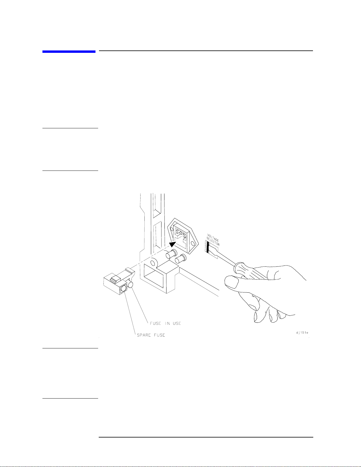
Quick Start Guide
Turning the Spectrum Analyzer On for the First Time
Turning the Spectrum Analyzer On for the
First Time
The spectrum analyzer requires no installation other than connection
to an ac power source. If you want to install your spectrum analyzer
into an HP System II cabinet or a standard 19 inch (486.2 mm)
equipment rack, complete instructions are provided with the Option
908 and Option 909 Rack mounting Kits.
CAUTION Do not connect the analyzer to an ac power source before verifying that
the line voltage is correct, the line-voltage selector switch located on the
analyzer rear panel is set to the correct voltage, and the proper fuse is
installed. Failure to verify that these items are correct could result in
equipment damage.
Figure 1-2 Selecting the Correct Line Voltage
CAUTION When installing the instrument in a cabinet, the convection into and
out of the instrument must not be restricted. The ambient temperature
(outside the cabinet) must be less than the maximum operating
temperature of the instrument by 4 degrees C for every 100 watts of
power dissipated in the cabinet. If the total power dissipated in the
cabinet is greater than 800 watts, then forced convection must be used.
28 Chapter1
Page 29

Quick Start Guide
Turning the Spectrum Analyzer On for the First Time
1. Press LINE to turn the analyzer on.
2. The analyzer takes about half a minute to perform a series of
self-diagnostic and adjustment routines. At completion, the screen
displays the analyzer model number and the firmware date (for
example, 890802 indicates August 2, 1989). If you should ever need
to call Hewlett-Packard for service or have any questions regarding
your analyzer, it is helpful to know the firmware date to get the most
accurate information.
3. Allow the analyzer a 5-minute warmup. Refer to the warmup
specification in the calibration guide.
4. The reference level calibration adjustment procedure in this chapter
should be performed before checking the specifications.
5. The trace alignment procedure can be performed to optimize the
display location.
6. The HP-IB address may need to be changed for remote operation.
Chapter 1 29
Page 30
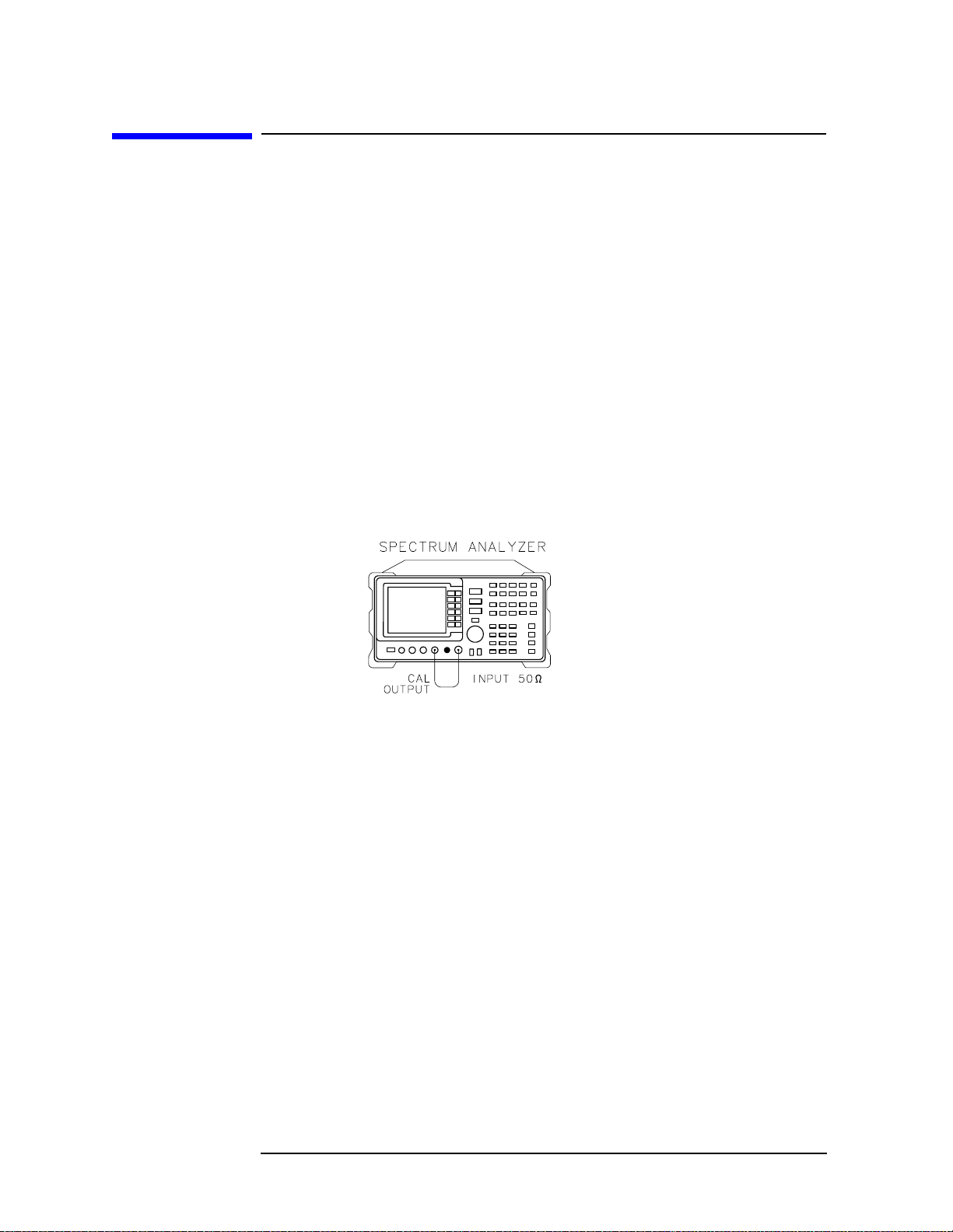
Quick Start Guide
Making a Basic Measurement
Making a Basic Measurement
A basic measurement involves tuning the spectrum analyzer to place a
signal on the screen, then measuring the frequency and amplitude of
the signal with a marker. We can measure an input signal in four
simple steps.
1. Set the center frequency.
2. Set the frequency span.
3. Activate the marker.
4. Set the amplitude.
As an example, we will measure the front panel 300 MHz calibration
signal. First, switch on the spectrum analyzer. (Formaximum accuracy,
if the analyzer has just been powered up, allow for a 5-minute warmup.)
Figure 1-3 300 MHz Calibration Signal Connection
Connect a short cable from the analyzer CAL OUTPUT connector to the
INPUT 50 Ω connector (both connectors are on the front panel of the
spectrum analyzer). Then perform the following steps:
1. Set the center frequency.
a. Press
FREQUENCY. This activates the center frequency function,
indicated by CENTER appearing in the active function block on the
left side of the display (see Figure 1-5 on page 31). It also brings
up a menu of other frequency functions. See Figure 1-4 on page
31.
These functions are called softkeys and are designated in the
manual by shading. (e.g.
CENTER FREQ) Most front panel keys
access menus of softkey functions.
30 Chapter1
Page 31

Figure 1-4 Softkey Menu
b. Toset the center frequency to 300 MHz, use the keys in the DATA
section of the front panel and enter 300 MHz. These data keys
allow you to select the exact numeric value of the active function,
which, in this case, is the center frequency. The step keys and
knob also allow you to select values for the function.
Quick Start Guide
Making a Basic Measurement
NOTE When entering some data values, such as unitless entries, ENTER must
be used to terminate the data entry.
ENTER is located in the lower right
corner of the spectrum analyzer front panel. It is also labeled Hz/µV/µs.
Figure 1-5 300 MHz Center Frequency
2. Set the frequency span.
a. Press
SPAN. Note that SPAN is now displayed in the active
function block, identifying it as the current active function.
b. To reduce the frequency span—for example, to 20 MHz—either
press 20 MHz on the data keypad, or use the
Chapter 1 31
⇓ key to "step down"
Page 32
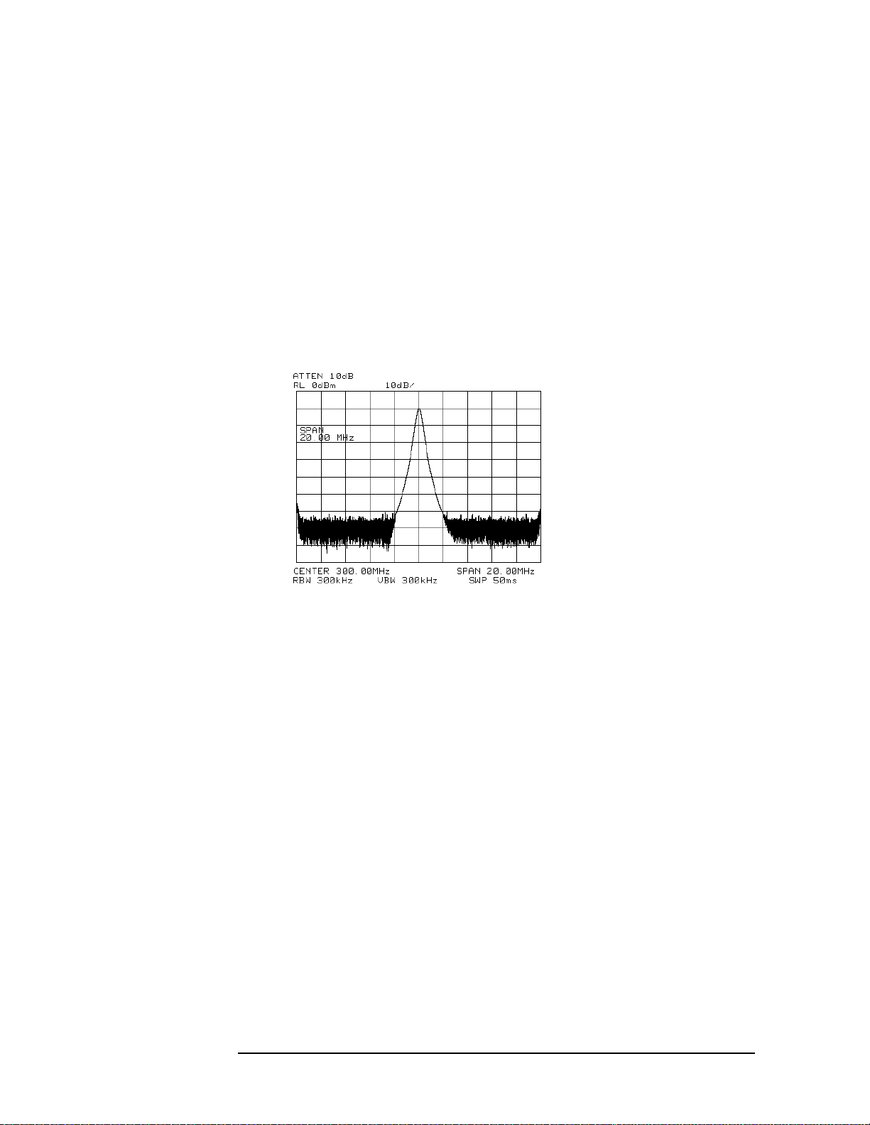
Quick Start Guide
Making a Basic Measurement
to this value. (Like data keys, step keys can also be used to
change the numeric value of the active function.)
The resulting display is shown in Figure 1-6. Note that the
resolution and video bandwidths are coupled to the frequency
span; they are automatically adjusted to appropriate values for a
given span. Sweeptime is also a coupled function.
c. Press
SWEEP and notice the SWP TIME AUTO MAN softkey. The
softkey can be used to make the sweeptime be auto-coupled or
manually controlled; the underline indicates which part of the
function is enabled. For example, the
function is auto-coupled when AUTO is underlined.
Figure 1-6 20 MHz Frequency Span
3. Activate the marker.
a. Press
MKR, which is located in the MARKER section of the front
panel. This activates the normal marker and places it at the
center of the trace (in this case, at or near the peak of the signal).
SWP TIME AUTO MAN
The marker reads both the frequency and the amplitude, and
displays these values in the active function block. In this case, the
marker reads 300.00 MHz and −10.00 dBm, as shown in Figure
1-7 on page 33.
b. If the marker is not on the peak of the signal, it can be placed on
the highest point by pressing
PEAK SEARCH, or by using the knob
to move the marker manually.
32 Chapter1
Page 33
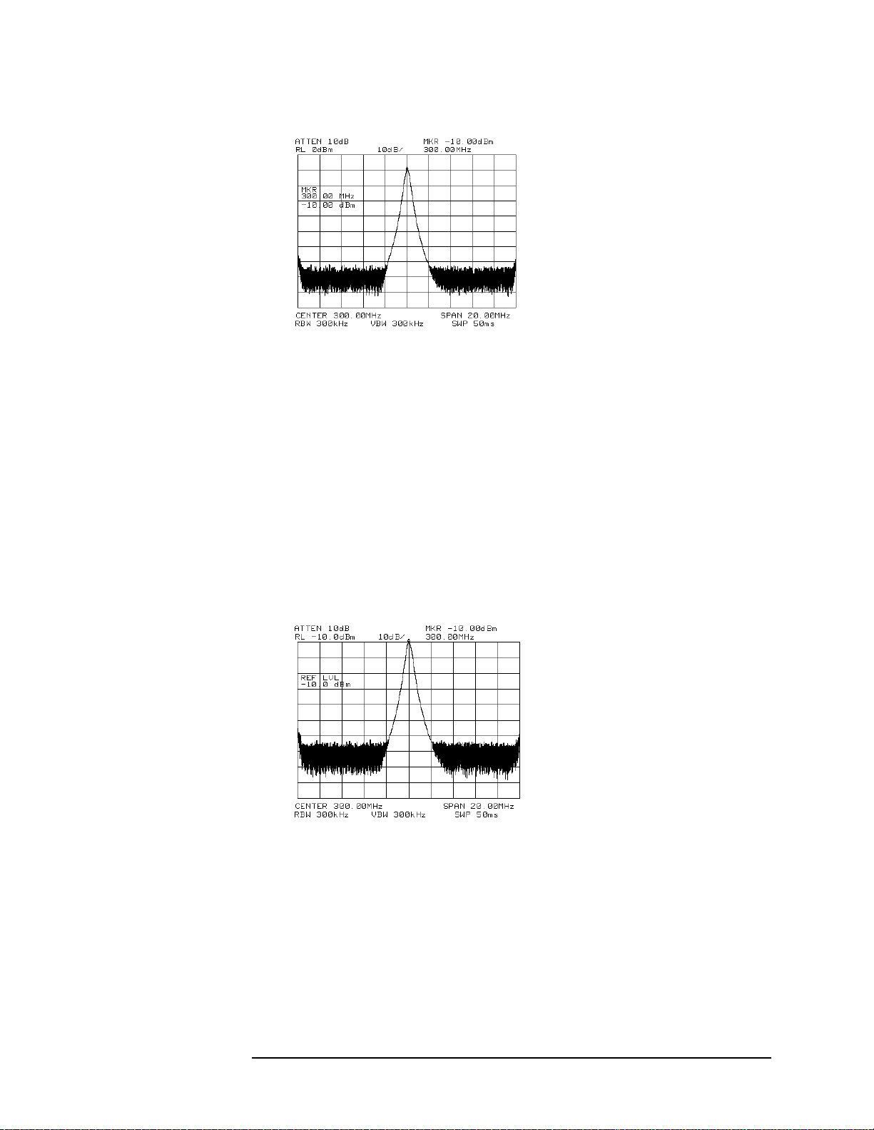
Figure 1-7 Activated Normal Marker
4. Set the amplitude.
a. Generally, placing the signal peak at the reference level provides
the best measurement accuracy. To adjust the signal peak to the
reference level ( Figure 1-8), press
dBm, or use either the step keys or the knob.
Using the knob is the easiest way to fine-tune the signal peak to
the reference level, which is located at the top of the graticule.
Quick Start Guide
Making a Basic Measurement
AMPLITUDE. Then key in −10
b. Because the marker is active, a faster method to fine-tune the
signal peak to the reference level is to press
which is located under the
reference level equal to the marker amplitude value.
Figure 1-8 −10 dBm Reference Level
MARKER → REF LVL,
MKR → key. This function sets the
Chapter 1 33
Page 34
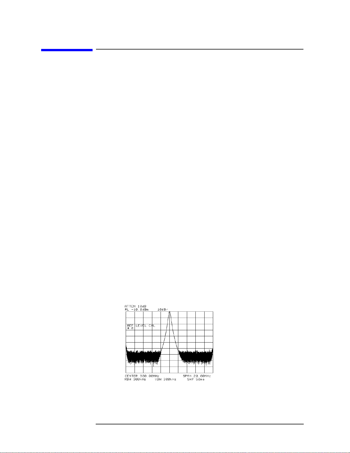
Quick Start Guide
Reference Level Calibration
Reference Level Calibration
Recalibrating the reference level is usually necessary only when the
ambient temperature changes more than 10 degrees Celsius. Because
the spectrum analyzer continually monitors and reduces any IF errors,
executing the reference-level calibration is seldom necessary.
The reference-level calibration function
REF LVL ADJ allows the
analyzer internal gain to be adjusted. When the calibrator signal is
connected to the input, selecting a reference level equal to the
calibrator amplitude will display the signal at top-screen.
1. Turn the markers off by pressing
2. Press
CAL. This accesses a menu of calibration routines. The fifth
function on this new list, labeled
MKR, then MARKERS OFF.
REF LVL ADJ, allows you to
calibrate the amplitude of the instrument.
3. Press REF LVL ADJ to activate the function.
4. To calibrate the spectrum analyzer, use the knob on the front panel
and adjust the peak of the signal to the reference level as shown in
Figure 1-9. Note the number that appears in the active function
block (number 0 in this example). This number ranges from −528 to
+528 (−33 to +33 in earlier instruments). It is a relative value
indicating how much amplitude correction was required to calibrate
the spectrum analyzer. The number is usually around 0.
If the amplitude is at either end of the range, or if it cannot be
adjusted to a value within this range, consult the calibration guide.
5. To store the value, press the
STORE REF LVL softkey. When entering
or storing a value using the data keys, the entry must be terminated
with the
ENTER key, located in the lower-right corner of the analyzer.
Figure 1-9 Peaked Signal to Reference Level
34 Chapter1
Page 35
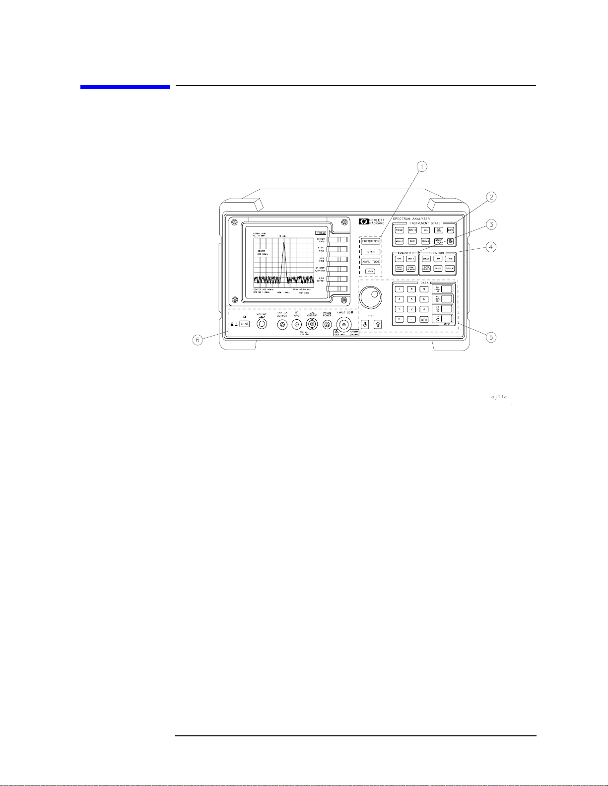
Quick Start Guide
Front Panel Overview
Front Panel Overview
Figure 1-10 Front Panel of an HP 8560 E-Series or EC- Series Spectrum
Analyzer
1. FREQUENCY, SPAN, and AMPLITUDE are the fundamental
functions for most measurements. The HOLD key freezes the active
function and holds it at the current value until a function key is
pressed.
2. INSTRUMENT STATE functions affect the state of the entire
spectrum analyzer, not just the state of a single function.
3. MARKER functions read out frequencies and amplitudes on the
spectrum analyzer trace, let you make relative measurements,
automatically locate the signal of highest amplitude on a trace, and
tune the spectrum analyzer to track a signal automatically.
4. CONTROL functions allow you to adjust the resolution and video
bandwidths, the sweep time, the display, and other functions that
control spectrum analyzer measurement capabilities.
5. DATA keys, STEP keys, and the knob allow you to change the
numeric value of the active function. Use the data keys to enter an
exact value or to move quickly from one value to another. The step
keys vary a value in predefined increments or, for some functions, in
increments that you choose. The knob allows you to fine-tune most
numeric values.
Chapter 1 35
Page 36

Quick Start Guide
Front Panel Overview
6. The front-panel connectors include an RF input, an active-probe
power, a 300 MHz calibrator signal, a 310.7 MHz IF input, and a
first LO output. Table 1-2 has a short specification summary of these
connectors. The IF input is not available with the HP 8560E/EC,
Option 002. A volume knob is provided for making adjustments to
the volume of the built-in speaker. The LINE button turns the
spectrum analyzer on and off.
CAUTION The maximum input level to the INPUT 50 Ω is +30 dBm with a
minimum of 10 dB input attenuation.
For the HP 8560E/EC, HP 8561E/EC, or HP 8562E/EC only: When ac
coupled, the maximum dc voltage to the RF input is ±50 V. When dc
coupled, the maximum dc voltage is ±0.2 V. Default power-up mode is ac
coupled. It is best to leave the analyzer in ac coupled mode for
maximum protection. Exceeding the maximum safe input levels can
damage the input attenuator and the input mixer.
For the HP 8563E/EC, HP 8564E/EC, or HP 8565E/EC only: The
maximum dc voltage to the RF input is ±0.2 V. Exceeding this voltage
can damage the input attenuator and the input mixer. Option 006
extends the frequency range down to 30 Hz and is more susceptible to
damage from dc voltages.
36 Chapter1
Page 37

Table 1-2
Quick Start Guide
Front Panel Overview
Connector Frequency Range Amplitude/ Voltage
Limits
INPUT 50 Ω HP 8560E/EC:
30 Hz–2.9 GHz (dc coupled)
100 kHz–2.9 GHz (ac coupled)
HP 8561E/EC:
30 Hz–6.5 GHz (dc coupled)
100 kHz–6.5 GHz (ac coupled)
HP 8562E/EC:
30 Hz–13.2 GHz (dc coupled)
100 kHz–13.2 GHz (ac coupled)
HP 8563E/EC:
9 kHz–26.5 GHz (dc coupled)
30 Hz–26.5 GHz (Option 006)
HP 8564E/EC:
9 kHz–40 GHz (dc coupled)
30 Hz–40 GHz (Option 006)
HP 8565E/EC:
9 kHz–50 GHz (dc coupled)
30 Hz–50 GHz (Option 006)
PROBE POWER —— +15 V, −12.6 V (150 mA max)
CAL OUTPUT 300 MHz −10 dBm
IF INPUT*
(foruse with external
mixers)
310.7 MHz 0 V dc Max
+30 dBm Max
±0.2 V dc Max (dc coupled)
±50 V dc Max (ac coupled)
+30 dBm Max
±0.2 V dc Max (dc coupled)
±50 V dc Max (ac coupled)
+30 dBm Max
±0.2 V dc Max (dc coupled)
±50 V dc Max (ac coupled)
+30 dBm Max
±0.2 V dc Max (dc coupled)
+30 dBm Max
±0.2 V dc Max (dc coupled)
+30 dBm Max
±0.2 V dc Max (dc coupled)
1ST LO
OUTPUT
RF OUT 50 Ω†
(tracking generator
output)
* Not available with an HP 8560E/EC Option 002 or Option 327.
† Available only with an HP 8560E/EC Option 002.
‡ LO output of an HP 8560E/EC Option 002.
Chapter 1 37
3.00 GHz–6.81 GHz +16.5 dBm ±2.0 dB
+14.5 dBm ± 3.0 dB‡
300 kHz–2.9 GHz −10 dBm to +1 dBm
Page 38
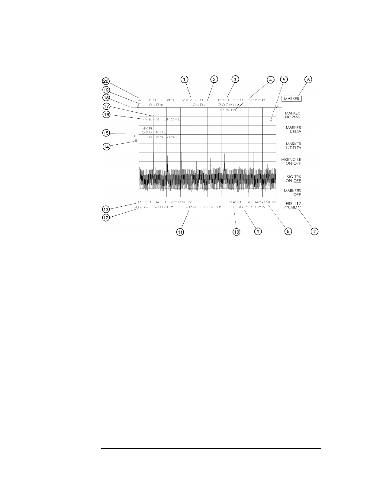
Quick Start Guide
Front Panel Overview
Display Annotation
Figure 1-11 Display Annotation
1. Number of video averages.
2. Logarithmic or linear amplitude scale per division.
3. Marker amplitude and frequency.
4. Title area.
5. Data invalid indicator, displayed when analyzer settings are
changed before completion of a full sweep.
6. Menu title and softkey menu.
7. Error message area.
8. Frequency span or stop frequency.
9. Sweep time.
10.Indicator of uncoupled function for sweep time, resolution
bandwidth, video bandwidth, or input attenuation.
11.Video bandwidth.
12.Resolution bandwidth.
13.Center or start frequency.
38 Chapter1
Page 39

Table 1-3
Quick Start Guide
Front Panel Overview
14.Active special functions: the following characters appear in a
vertical line alongside the graticule. This information is also
available by pressing
A = IF adjust turned OFF
C = DC coupling selected (The HP 8563E/EC, HP 8564E/EC, and HP
8565E/EC are always dc coupled. AC coupling is available only for
an HP 8560E/EC, HP 8561E/EC or HP 8562E/EC spectrum
analyzers. The default setting for an HP 8560E/EC, HP 8561E/EC
or HP 8562E/EC is ac coupling.)
D = Detector mode set to sample, negative peak, or positive peak
E = Special sweep-time equations in use (refer to tracking generator
menus)
F = Frequency offset is less than or greater than 0 Hz
G = Internal tracking generator is ON
DISPLAY, then ANNOT HELP.
K = Signal track is ON
M = Trace math is ON
N = Normalization is ON
R = Reference level offset is less than or greater than 0 dB
S = Single-sweep mode
T = Trigger mode set to line, video, or external
W = Amplitude correction (ampcor) is on
X = 10 MHz reference is external
+ = External mixer bias is greater than 0 mA
− = External mixer bias is less than 0 mA
15.Active function area
16.Message area (for example, messages such as MEAS UNCAL, PEAKING,
and Sampling are displayed in the message area)
17.Marker indicator
18.Indicator of reference-level position when in normalized mode
19.Reference level
20.Input attenuator value (internal mixing) or conversion loss (external
mixing)
Chapter 1 39
Page 40
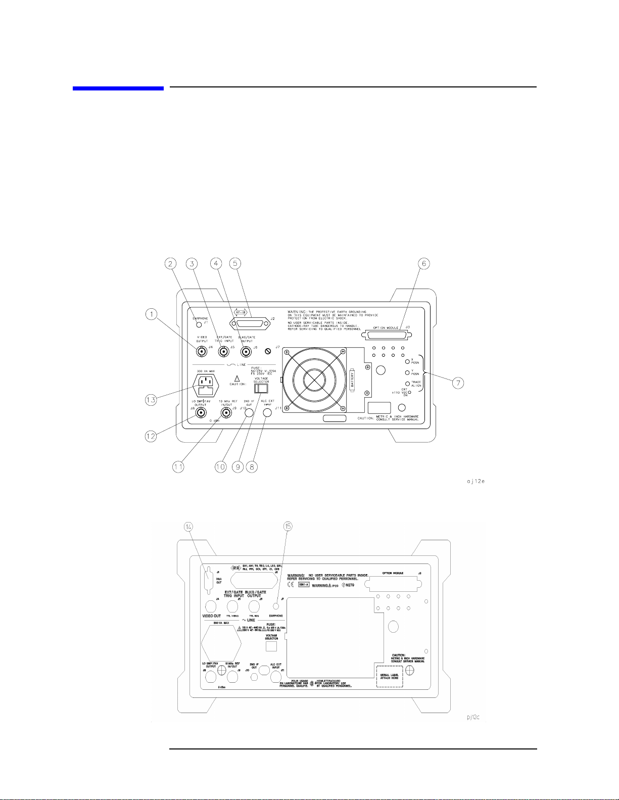
Quick Start Guide
Rear Panel Overview
Rear Panel Overview
The rear panels of the E-series and EC-series are identical except
the earjack on the E-series instruments is located at J1 (see 2, Figure
1-12) while on EC-series instruments, the earjack is located at J7 (see
15, Figure 1-13). EC-series instruments have a VGA port at J1, while
E-series instruments do not have a VGA port. Three CRT display
adjustment pots are accessed through the rear of E-series instruments
(see 7, Figure 1-12), which are not present on EC-series instruments.
Figure 1-12 Rear Panel Functions - 8560 E-series
Figure 1-13 Rear Panel Functions - 8560 EC-series
40 Chapter1
Page 41

Quick Start Guide
Rear Panel Overview
CAUTION Toprevent damage to the instrument, be sure to set the voltage selector
to the appropriate value for your local line-voltage output. For more
information, refer to the "If You Have A Problem" chapter.
1. J4 VIDEO OUTPUT provides a detected video signal that is
proportional to the vertical deflection of the trace on the display. The
output range is 0 V to 1 V when terminated in 50 Ω. It can be used
when the display is in 10 dB/div or LINEAR mode. For resolution
bandwidth settings less than 300 Hz, a 4.8 kHz IF signal with a dc
offset is present at J4. The VIDEO OUTPUT connector is not
available with Option 327.
2. J1 on 8560 E-series instruments (see 14 for information on J1 in
EC-series instruments) EARPHONE provides a 4 Ω impedance
earphone jack .
3. J5 EXT/GATE TRIG INPUT accepts a TTL signal as an external
trigger, or as a trigger for gated video. The input signal range is 0 V
to 5 V (TTL). For external triggering, the instrument sweep triggers
on the rising or falling edge (as determined by
TRIG POL POS NEG)of
the signal (about +1.5 V).
For gated video triggering, the instrument sweep trigger depends upon
the setting of
GATE CTL EDGE LVL. If GATE CTL EDGE LVL is set to
EDGE, either the positive or negative edge of the trigger input
signal initiates the gate delay. (Set
GATE CTL EDGE LVL is set to level (LVL),either the TTL high level or
TTL low level opens the gate. (Set
control functions can be accessed by pressing
EDGE POL POS NEG.) If
LVL POL POS NEG.) The gate
SWEEP.
4. J6 BLKG/GATE OUTPUT provides either a blanking output or a
gate output.
The blanking output is a 0 V to 5 V (TTL) signal that is low (0 V)
during spectrum analyzer sweeps. The output is high (5 V) during
retrace and when the instrument is between bands in multiband
sweeps. Use this output for pen lift when plotting with nondigital
plotters. It is also useful for synchronizing instruments.
The gate output provides a TTL signal that indicates the status of
the gate when the gate is in edge trigger mode. A high TTL signal
indicates the gate is on; a low TTL signal indicates the gate is off.
The gate output is not active in level mode.
5. J2 HP-IB is the Hewlett-Packard Interface Bus connector.
6. J3 OPTION MODULE allows connection of option modules such as
the HP 85620A mass memory module or the HP 85629B test and
adjustment module.
7. X POSN, Y POSN, and TRACE ALIGN on 8560 E-series
instruments allow you to align the spectrum analyzer display of
Chapter 1 41
Page 42

Quick Start Guide
Rear Panel Overview
using a special CRT pattern. Refer to the softkey CRT ADJ PATTERN
under the CAL menu, or consult the service guide for your model of
spectrum analyzer. 8560 EC-Series instruments are not adjustable.
8. J11 ALC EXT INPUT provides either an external leveling input or
an alternate sweep output that corresponds to the sweep ramp that
tunes the local oscillator.
For an HP 8560E/EC, Option 002 (which has a built-in tracking
generator), J11 provides an external leveling input. For an Option
005, J11 provides a 0 V to 10 V ramp that corresponds to the sweep
ramp that tunes the local oscillator (the same local oscillator sweep
ramp that J8 provides).
9. VOLTAGE SELECTOR switchadapts the spectrum analyzer to the
power source: either 115 V or 230 V.
10.J10 2ND IF OUT is the Option 001, 310.7 MHz IF output.
11. J9 10 MHz REF IN/OUT provides a 10 MHz, 0 dBm minimum,
time-base reference signal. This connector can be switched to an
input, to use an external reference. An external reference must be 10
MHz at a minimum of −2 dBm. To select the external reference
mode, press
AUX CTRL, REAR PANEL, 10 MHZ EXT INT.
12. J8 LO SWP|FAV OUTPUT provides different signals at connector
J8: a 0 V to 10 V ramp corresponding to the local oscillator tune
ramp, or a sweeping dc output of 0.5 V per GHz of tuned frequency
(and 0.25 V for the HP 8564E/EC and HP 8565E/EC). The voltage
range of the sweeping dc output depends on the spectrum analyzer
frequency range. Select the output with the softkeys that are
accessed when you press
AUX CTRL, REAR PANEL.
The 0.25 V/GHz output is needed for frequency ranges above 26
GHz. External tracking generators, such as the HP 85640A, HP
85644A, or HP 85645A use the 0.5 V/GHz output. When you have
selected preselected external mixers, the 0.5 V/GHz output provides
approximately 1.5 V per GHz of LO frequency, to control the
preselected mixer.
13.The LINE input operates at nominally 115 V (47 to 440 Hz) or at
nominally 230 V (47 to 66 Hz).
14.J1 VGA OUT port on 8560 EC-series instruments provides a VGA
port. The VGA port is always active and does not require user
interface.
15. J7 EARPHONE provides a 4 Ω impedance earphone jack on 8560
EC-series instruments.
42 Chapter1
Page 43

Quick Start Guide
Assistance
Assistance
Product maintenance agreements and other customer assistance
agreements are available for Hewlett-Packard products.
For any assistance, contact your nearest Hewlett-Packard Sales and
Service Office.
Cleaning
The instrument front and rear panels should be cleaned using a soft
cloth with water or a mild soap and water mixture.
Safety Symbols
The following safety symbols are used throughout this manual.
Familiarize yourself with each of the symbols and its meaning before
operating this instrument.
CAUTION The caution sign denotes a hazard. It calls attention to a procedure
which, if not correctly performed or adhered to, could result in damage
to or destruction of the instrument. Do not proceed beyond a caution
until the indicated conditions are fully understood and met.
WARNING The warning sign denotes a hazard. It calls attention to a
procedure which, if not correctly performed or adhered to,
could result in injury or loss of life. Do not proceed beyond a
warning until the indicated conditions are fully understood
and met.
Instruction
Documentation
The product is marked with this symbol when it is
necessary for you to refer to the instructions in the
documentation.
Chapter 1 43
Page 44

Quick Start Guide
General Safety Considerations
General Safety Considerations
WARNING Before this instrument is switched on, make sure it has been
properly grounded through the protective conductor of the ac
power cable to a socket outlet provided with protective earth
contact.
Any interruption of the protective (grounding) conductor,
inside or outside the instrument, or disconnection of the
protective earth terminal can result in personal injury.
If this instrument is used in a manner not specified by
Hewlett-Packard Co., the protection provided by the
instrument may be impaired.
There are many points in the instrument which can, if
contacted, cause personal injury. Be extremely careful. Any
adjustments or service procedures that require operation of the
instrument with protective covers removed should be
performed only by trained service personnel.
CAUTION Before this instrument is switched on, make sure its primary power
circuitry has been adapted to the voltage of the ac power source.
Failure to set the ac power input to the correct voltage could cause
damage to the instrument when the ac power cable is plugged in.
This product conforms to Enclosure Protection IP 2 0 according to
IEC-529. The enclosure protects against finger access to hazardous
parts within the enclosure; the enclosure does not protect against the
entrance of water.
44 Chapter1
Page 45

Quick Start Guide
HP 8560 E-Series and EC-Series Spectrum Analyzer Documentation Description
HP 8560 E-Series and EC-Series Spectrum
Analyzer Documentation Description
User's Guide
The HP 8560 E-Series and EC-Series User's Guide applies to the HP
8560E/EC, HP 8561E/EC, HP 8562E/EC, HP 8563E/EC, HP 8564E/EC,
and HP 8565E/EC spectrum analyzers. The HP 8560 E-Series and
EC-Series User's Guide includes information about preparing the
spectrum analyzer for use, spectrum analyzer functions, common
spectrum analyzer measurements, programming fundamentals, and
definitions for remote programming commands.
In addition to the user's guide, the following manuals are shipped with
your spectrum analyzer:
Calibration Guide
The HP 8560 E-Series and EC-Series Calibration Guide includes the
specifications and characteristics, and information about how to test
your spectrum analyzer to determine if the spectrum analyzer meets its
specifications.
Quick Reference Guide
The HP 8560 E-Series and EC-Series Quick Reference Guide applies to
the HP 8560E/EC, HP 8561E/EC, HP 8562E/EC, HP 8563E/EC, HP
8564E/EC, and HP 8565E/EC spectrum analyzers. The HP 8560
E-Series and EC-Series Quick Reference Guide includes information
about how to make a simple measurement with your spectrum
analyzer, briefly describes the spectrum analyzer functions,and lists all
the programming commands.
Chapter 1 45
Page 46

Quick Start Guide
Manuals Available Separately
Manuals Available Separately
Service Guide
The service guide provides information for servicing an instrument to
the assembly level. The manual includes instrument adjustments,
troubleshooting, major assembly replaceable parts lists, and
replacement procedures. For ordering information, contact a
Hewlett-Packard Sales and Service Office. This manual is not always
immediately available for new products.
Component-Level Information
The component-level information manual provides component level
information for the assemblies used in the instrument. Schematic
drawings, component locators and assembly parts list are provided for
the current vintage of assemblies. Component-level information is not
always immediately available for new assemblies.
How to Order Manuals
Each of the manuals listed above can be ordered individually. To order,
contact your local HP Sales and Service Office. See Table 9-3 on
page 679 for a listing of HP sales and service offices.
46 Chapter1
Page 47

2 Making Measurements
47
Page 48

Making Measurements
Making Measurements
Making Measurements
This chapter demonstrates spectrum analyzer measurement
techniques with examples of typical applications. Each application
focuses on different features of the HP 8560 E-Series and EC-Series
spectrum analyzers. The measurement application and procedures
covered in this chapter are:
• Resolving Closely Spaced Signals (with Resolution Bandwidth)
• Improving Amplitude Measurements with Ampcor
• Modulation
• Harmonic Distortion
• Third-Order Intermodulation Distortion
• AM and FM Demodulation
• Stimulus-Response Measurements
• External Millimeter Mixers
• Adjacent Channel Power Measurement
• Power Measurements Functions
• Time-gated Measurement
• Making Time-Domain Measurements Using Sweep Delay
• Making Pulsed RF Measurements
48 Chapter2
Page 49

Making Measurements
Example 1: Resolving Closely Spaced Signals (with Resolution Bandwidth)
Example 1: Resolving Closely Spaced Signals
(with Resolution Bandwidth)
What Is Resolution Bandwidth?
Signal resolution is determined by the intermediate frequency (IF)
filter bandwidth. The spectrum analyzer traces the shape of its IF filter
as it tunes past a signal. Thus, if two equal-amplitude signals are close
enough in frequency, the filter shapes for the two signals can fall on top
of one another and appear as a single response. If two signals are not
equal in amplitude but are still close together,the smaller signal can be
hidden under the response of the larger one.
Spectrum Analyzer Function Used
The resolution bandwidth function (RESBW)selects the appropriate IF
bandwidth for a measurement. (Hewlett-Packard specifies resolution
bandwidth as the 3 dB bandwidth of a filter.) The following guidelines
can help you determine the appropriate resolution bandwidth to choose.
Stepping Through a Measurement of Two Equal
Amplitude Signals
Generally, to resolve two signals of equal amplitude, the resolution
bandwidth must be less than or equal to the frequency separation of the
two signals. For example, to resolve two signals of equal amplitude with
a frequency separation of 1 kHz, a resolution bandwidth of 1 kHz or less
should be used.
1. Connect two signal sources to the spectrum analyzer INPUT 50 Ω.
Set the frequency of one source to 499.5 kHz and the other source to
500.5 kHz. Set both sources to the same amplitude.
2. Press
a preset state,and set the spectrum analyzer center frequency to 500
kHz.
3. Set the span to 10 kHz.
4. Set the resolution bandwidth to 1 kHz. See Figure 2-1.
5. Change the resolution bandwidth to a wider value and notice that
you can no longer see that there are two signals present.
6. Change the two source frequencies to 499 kHz and 501 kHz.
PRESET on the spectrum analyzer to start the procedure from
Chapter 2 49
Page 50

Making Measurements
Example 1: Resolving Closely Spaced Signals (with Resolution Bandwidth)
To resolve two signals with a frequency separation of 2 kHz, a 1 kHz
resolution bandwidth again must be used (see Figure 2-2). Since the
spectrum analyzer uses bandwidths in a 1, 3, 10 sequence, the next
larger filter, 3 kHz, would exceed the 2 kHz separation and thus would
not resolve the signals.
Keep in mind that noise sidebands (phase noise) can also affect
resolution.
Figure 2-1 1 kHz Signal Separation
Figure 2-2 2 kHz Signal Separation
50 Chapter2
Page 51

Making Measurements
Example 1: Resolving Closely Spaced Signals (with Resolution Bandwidth)
Stepping Through a Measurement of Two Signals of
Unequal Amplitude
This example resolves a third-order intermodulation distortion product
with a frequency separation of 700 kHz and an amplitude separation of
about 60 dB.
1. Connect two signal sources to the spectrum analyzer INPUT 50 Ω.
Set the frequency of one source to 10 MHz and the other source to
10.7 MHz. Set both sources to an amplitude of about −10 dBm.
2. Press
a preset state and set the spectrum analyzer center frequency to
10.35 MHz.
3. Set the span to 5 MHz.
4. Set the resolution bandwidth to 100 kHz and the video bandwidth to
1 kHz. See Figure 2-4 on page 53.
To resolve two signals of unequal amplitude, the resolution bandwidth
must be less than or equal to the frequency separation of the two
signals (the same as resolving two equal amplitude signals). However,
in this case the largest resolution bandwidth that will resolve the two
unequal signals is determined primarily by the shape factor of the IF
filter, rather than by the 3 dB bandwidth. Shape factor is defined as the
ratio of the 60 dB bandwidth to the 3 dB bandwidth of the IF filter,as in
Figure 2-3.
The wider IF filters in this spectrum analyzer have shape factors of
15:1 or better. The IF filters less than or equal to 100 Hz have a better
shape factor of 5:1 or better. Therefore, to resolve two signals of unequal
amplitude, the half-bandwidth of a filter at the point equal to the
amplitude separation of the two signals must be lessthanthe frequency
separation of the two signals.
PRESET on the spectrum analyzer to start the procedure from
Chapter 2 51
Page 52
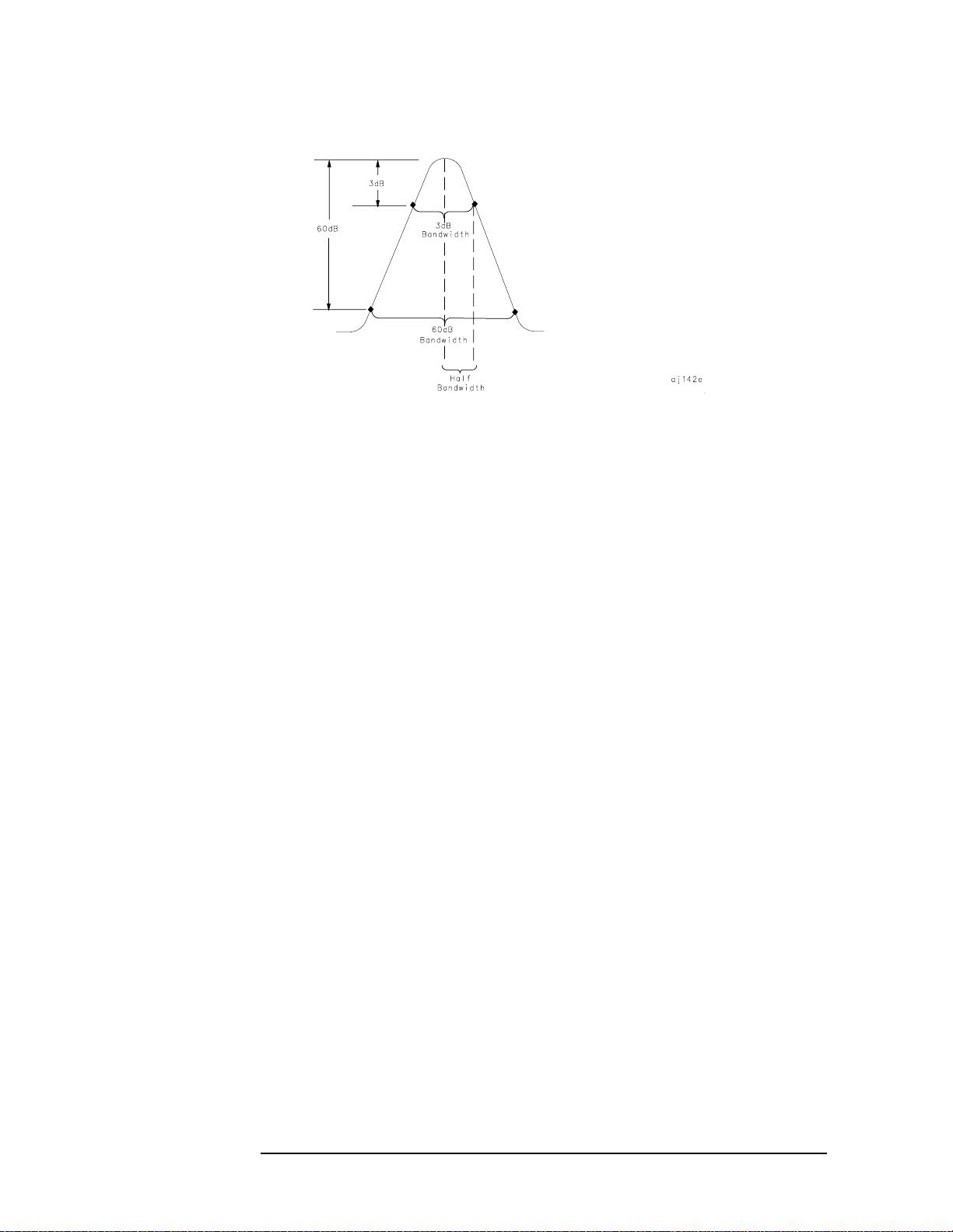
Making Measurements
Example 1: Resolving Closely Spaced Signals (with Resolution Bandwidth)
Figure 2-3 Bandwidth Shape Factor
Use a 100 kHz resolution bandwidth filter to resolve this third-order
intermodulation distortion product. The 100 kHz filter has a typical
shape factor of 12:1, a 60 dB bandwidth of 1.2 MHz, and a
half-bandwidth value of 600 kHz. This half-bandwidth isnarrower than
the frequency separation, so the two input signals will be resolved. See
Figure 2-4.
However, using a 300 kHz filter, the 60 dB bandwidth is 3.6 MHz and
the half-bandwidth value is 1.8 MHz. Since this half-bandwidth is
wider than the frequency separation, the signals most likely would not
be resolved
• Change the resolution bandwidth to 300 kHz and notice that you can
no longer see that the distortion product is present. See Figure 2-5
on page 53.
52 Chapter2
Page 53

Example 1: Resolving Closely Spaced Signals (with Resolution Bandwidth)
Figure 2-4 100 kHz Bandwidth Resolution
Figure 2-5 300 kHz Bandwidth Resolution
Making Measurements
NOTE Spectrum analyzer sweep time is inversely proportional to the square of
the resolution bandwidth, for bandwidths greater than or equal 300 Hz.
So, if the resolution bandwidth is reduced by a factor of ten, the sweep
time is increased by a factor of 100. Forfastest measurement times, use
the widest resolution bandwidth that still permits resolution of all
desired signals.
Chapter 2 53
Page 54

Making Measurements
Example 2: Improving Amplitude Measurements with Ampcor
Example 2: Improving Amplitude
Measurements with Ampcor
What Is Ampcor?
The amplitude correction function is used to improve the amplitude
accuracy of your measurement system. System flatness is often
degraded by many things includingcable and adapter losses. Additional
systematic amplitude errors such as IF gain uncertainty, resolution
bandwidth switching uncertainty, and attenuator switching
uncertainty can also be corrected. These system effects can be
normalized out of the displayed measurement results using the ampcor
function. Pairs of frequency/amplitude correction points are entered
into the spectrum analyzer. Turning on the ampcor function causes
real-time correction of the measurement data using these points. This
real-time correction is updated as the frequency and amplitude
parameters of the spectrum analyzer are changed.
Spectrum Analyzer Functions Used
This example uses the amplitude correction function, ampcor. It
illustrates the use of some of the ampcor data entry and editing
functions that help with the entry of the frequency-amplitude
correction pairs. Once you have entered a set of correction values, they
can be saved and recalled for later use.
Stepping Through an Ampcor Measurement
The ampcor function will be used to correct for variations in the flatness
of a measurement system. Suppose we want to make measurements on
a personal digital cellular system (PDC). The PDC frequency range is 1
GHz to 1.6 GHz, and in this frequency range the spectrum analyzer
frequency response has a small amount of ripple. The ampcor function
will be used to correct for this and for some cable losses.
Substitute a source and power meter for the PDC signal and set up the
measurement with the system cable. The flatness correction values are
identified, and then entered and saved.
54 Chapter2
Page 55
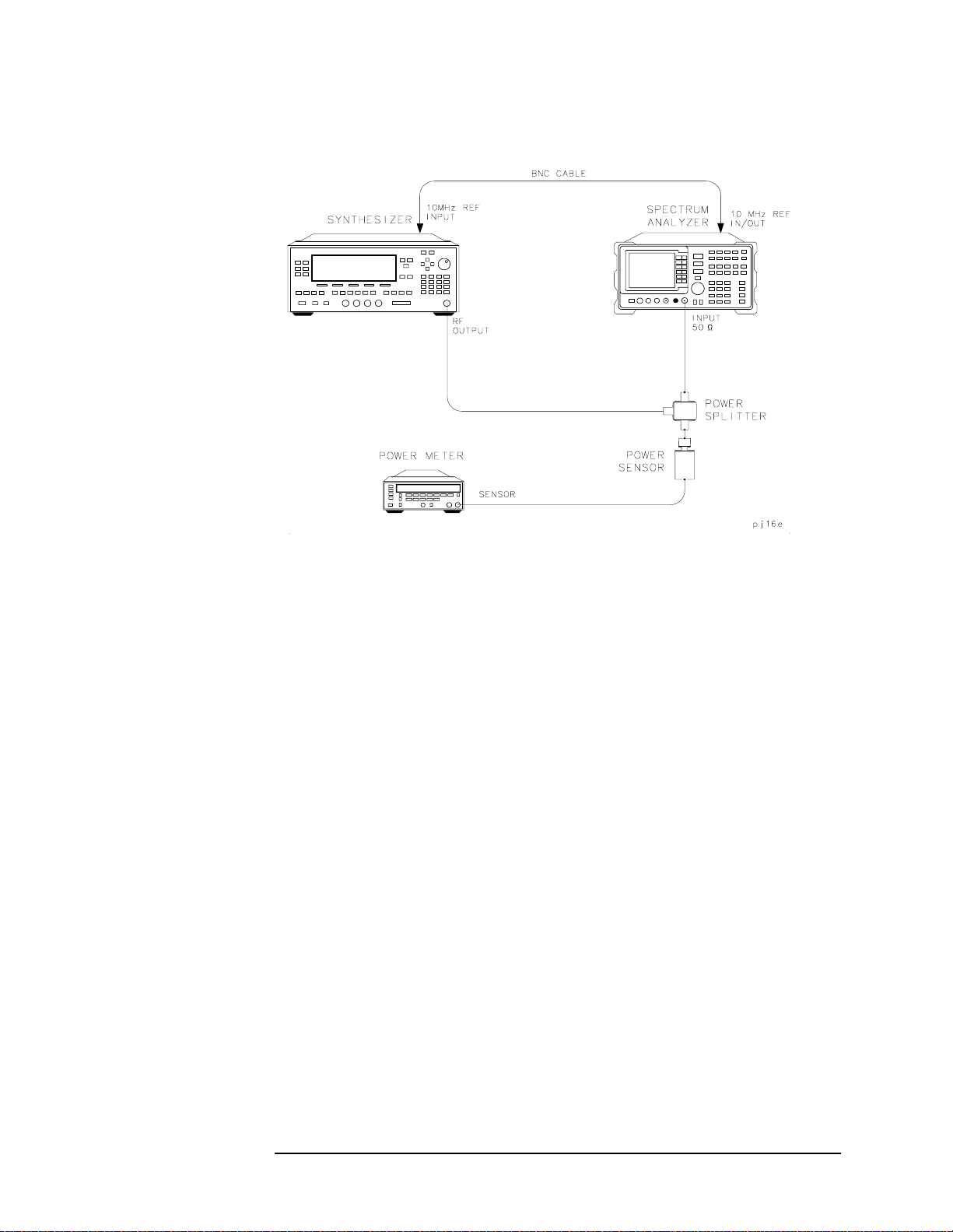
Example 2: Improving Amplitude Measurements with Ampcor
Figure 2-6 Ampcor Measurement Setup
Making Measurements
Set up the measurement.
1. Zero and calibrate the power meter and power sensor.
2. Connect the source output to the power splitter input. Connect the
system cable from the spectrum analyzer input to one of the power
splitter outputs. Connect the power sensor to the other power
splitter output. See Figure 2-6.
3. Set the source output to:
CW ............................................................................1.0 GHz
Amplitude................................................................... 0 dBm
4. On the power meter, enter the 1 GHz power sensor calibration factor.
5. The correction values should be determined using the same
measurement setup as the intended measurement will use. For the
purpose of this example, we will use the following spectrum analyzer
setup:
Center frequency......................................................1.0 GHz
Frequency span .........................................................5 MHz
Resolution bandwidth ............................................ 300 kHz
Log scale .......................................................... 1 dB/division
Chapter 2 55
Page 56

Making Measurements
Example 2: Improving Amplitude Measurements with Ampcor
6. On the spectrum analyzer, press CAL, MORE 1 OF 2, AMPCOR MENU,
and
EDIT AMPCOR. If there is a correction already loaded, purge it by
pressing
MORE 1 OF 2, DONE EDIT, PURGE CORR, PURGE DATA. (Or
you can save the correction first and then purge it. Refer to the
procedures that follow.) If data was purged, press
EDIT AMPCOR
again before continuing.
Enter the correction points.
1. On the spectrum analyzer, press
2 OF 2.
MORE 1 OF 2, PEAK SEARCH, MORE
2. Enter the marker frequency.
3. Use the knob to adjust AMPL until the marker amplitude reads the
same as the power meter.The ampcor function will be automatically
turned on after the first point is entered. Note the "W" along the left
edge of the display.
4. Set the source CW frequency to the next frequency to be corrected.
5. Enter the power sensor calibration factor for this frequency into the
power meter.
6. On the spectrum analyzer, press
FREQUENCY and enter the next
frequency to be corrected.
7. Press CAL, MORE 1 OF 2, AMPCOR MENU, EDIT AMPCOR, MORE 1 OF
2, PEAK SEARCH, MORE 2 OF 2, NEW CORR PT.
8. Use the knob to adjust AMPL until the marker amplitude reads the
same as the power meter.
9. Repeat steps 4 through 8 for each additional correction point.
Storing the ampcor data.
1. Press
MORE 1 OF 2, DONE EDIT, SAVE AMPCOR. Select a convenient
register number.
2. If you would like to create a softkey label under which the correction
data will be saved, press
the ampcor menu, press
DISPLAY and enter a screen title. Return to
SAVE AMPCOR and select a correction
register number. The first 16 characters of the screen title will be
used as a softkey label.
You have now completed the process for entering amplitude correction
points. At this point you can disconnect the source from the spectrum
analyzer input and connect the test signal, using the same system
cable. You can recall the correction points and begin to make
measurements.
56 Chapter2
Page 57

Making Measurements
Example 2: Improving Amplitude Measurements with Ampcor
Using the ampcor data.
1. With ampcor on, the amplitude measured by the analyzer at the
correction-point frequencies should agree with the power meter
reading ±0.2 dB. This error is due primarily to the spectrum
analyzer marker amplitude resolution, which ranges from 0.017 dB
to 0.17 dB, depending upon the log scale selected.
2. If you want to turn off ampcor,press
AMPCOR ON OFF so that OFF is
selected. The correction to the trace is now turned off, but the
correction values remain in memory.
3. If you want to purge the ampcor correction data, press
PURGE CORR
and purge the correction data. The correction values are now gone
from active memory.
Ampcor Limitations
When using the ampcor function consider the following:
Trace data above or below the graticule
If any of the uncorrected trace data is above or below
the graticule, the ampcor function will not properly
correct it. The spectrum analyzer amplitude accuracy is
not specified above or below the graticule. Anytime
ampcor applies a correction such that data outside the
graticule is moved to within the graticule, an error
(error number 921 or 922) is generated. In order to
avoid these errors, make sure that the trace data which
is being corrected is within the graticule before the
correction is applied.
Measurements near the bottom of the graticule
If you are using 10 dB/division and the measurements
occur in the bottom division of the display, imperfect log
fidelity will cause errors in the correction.
Flatness correction and temperature drift
If the factors that contribute to poor flatness are
temperature dependent, the corrections will not be as
effective.
Chapter 2 57
Page 58

Making Measurements
Example 3: Modulation
Example 3: Modulation
What Is Modulation?
Modulation is the act of translating some low frequency or baseband
signal (voice, music, data) to a higher frequency. In the modulation
process, some characteristic of a carrier signal (usually amplitude or
frequency) is changed in direct proportion to the instantaneous
amplitude of the baseband signal.
More information about amplitude and frequency modulation can be
found in Hewlett-Packard Application Note 150-1, literature number
5954-9130.
Spectrum Analyzer Functions Used
The following procedure describes how to measure signals with AM and
FM types of modulation on them. It shows how to tune the signal onto
the spectrum analyzer display. It demonstrates using the frequency
count function and several marker functions to make measurements.
Stepping Through Modulation Measurements
Amplitude Modulation
1. Connect the signal source to the spectrum analyzer INPUT 50Ω.
2. Set the source to a carrier frequency of 100 MHz with amplitude
modulation of about 34 kHz.
3. Set the spectrum analyzer center frequency to 100 MHz. Set the
span to 500 kHz.
4. Figure 2-7 on page 59 illustrates the amplitude-modulated signal as
seen on the spectrum analyzer display. Note the carrier signal. To
determine its frequency, simply press
5. Additional modulation information can be easily determined from
the carrier signal and a sideband. For example, the difference
between the carrier frequency and the sideband frequency can be
found by pressing
The markers read the frequency difference between the two signals,
which is equal to the modulating frequency. The marker also reads
the difference in amplitude. This difference in amplitude between
the two signals can be used to determine percentage of modulation
(refer to Figure 2-8 on page 59).
PEAK SEARCH, MARKER DELTA, and NEXT PEAK.
PEAK SEARCH.
58 Chapter2
Page 59

Figure 2-7 An Amplitude-Modulated Signal
Making Measurements
Example 3: Modulation
NOTE Unequal amplitudes of the lower and upper sidebands indicate
incidental FM on the input signal. Incidental FM can reduce the
accuracy of percentage-of-modulation measurements.
Figure 2-8 Percentage of Modulation
Chapter 2 59
Page 60

Making Measurements
Example 3: Modulation
The following equation also determines percentage of modulation using
amplitude units in volts:
100×
2A
M
s
------------------------=
A
c
where A
A
c
= sideband amplitude, in volts
s
= carrier amplitude, in volts
Frequency Modulation
This section contains general information about frequency modulation,
as well as a procedure for calculating FM deviation using a spectrum
analyzer.
For sinusoidal modulation where either the modulation frequency or
the FM deviation can be varied, the spectrum analyzer can be used to
accurately set up a modulation index corresponding to a Bessel null.
The following example illustrates how to verify the FM deviation
accuracy of a signal generator with FM capability. We will use a carrier
frequency of 100 MHz and test for FM deviation accuracy at a 25 kHz
rate using the modulation index for the first carrier null (2.401). Figure
2-9 illustrates how to set up the equipment for this measurement.
Figure 2-9 FM Deviation Test Setup
1. Connect the signal source to the spectrum analyzer INPUT 50Ω. Set
the source to 100 MHz.
2. Press
PRESET to begin with the spectrum analyzer in a preset state
and change the settings as follows:
a. Set center frequency to 100 MHz.
b. Set span to 100 kHz.
c. Set resolution bandwidth to 1 kHz.
d. Set video bandwidth to 1 kHz.
60 Chapter2
Page 61

Making Measurements
Example 3: Modulation
3. Figure 2-10 contains Bessel functions for determining modulation.
(Table 2-1 and Table 2-2 on page 61 also contain modulation index
numbers for carrier nulls and first sideband nulls.)
Figure 2-10 Bessel Functions for Determining Modulation Index
Table 2-1 Carrier Nulls and Modulation Indexes
Order of Carrier Null Modulation Index
1 2.401
2 5.520
3 8.653
4 11.791
5 14.931
6 18.071
n (n > 6) 18.071 + π(n − 6)
Table 2-2 Sideband Nulls and Modulation Indexes
Order of First Sideband Null Modulation Index
1 3.83
2 7.02
3 10.17
4 13.32
5 16.47
6 19.62
Chapter 2 61
Page 62

Making Measurements
Example 3: Modulation
4. Knowing that the desired deviation is 25 kHz, and choosing the
modulation index of the first carrier null, calculate the modulating
frequency as follows:
Modulating Frequency
Modulating Frequency 10.412kHz=
5. Set the modulation rate on the signal generator to 10.412 kHz. If the
signal source doesn't have an accurate internal modulation source,
use an external source. You can use the delta count mode of the
analyzer to accurately set the audio source frequency as follows:
Table 2-3
a. Press FREQ COUNT to activate the counter function, then press
COUNTER RES and set the counter resolution.
b. Press COUNTER ON OFF so that ON is underlined, and use the delta
count mode to read the difference between two sideband peaks (see
Figure 2-11).
25kHz
--------------- -=
2.401
c. Now adjust the frequency deviation for a maximum null of the carrier.
d. Calculate the FM deviation by multiplying the modulation index
(from Table 2-10) by the modulation rate:
e. FM Deviation = 10.39 kHz × 2.401
f. FM Deviation = 24.95 kHz
Figure 2-11 Markers Show Modulating Frequency
62 Chapter2
Page 63

• Gradually change the modulation frequency (or change the
amplitude of the modulation signal) and observe the changes in the
displayed nulls. Figure 2-12 illustrates a frequency-modulated
signal with a small modulation index (modulation index of about 0.2)
as it appears on a spectrum analyzer. Figure 2-13 on page 64 and
Figure 2-14 on page 64 illustrate larger modulation index values. In
the first figure the null is at the carrier.In the second figure the null
is at the first sideband.
Figure 2-12 A Frequency-Modulated Signal
Making Measurements
Example 3: Modulation
Chapter 2 63
Page 64
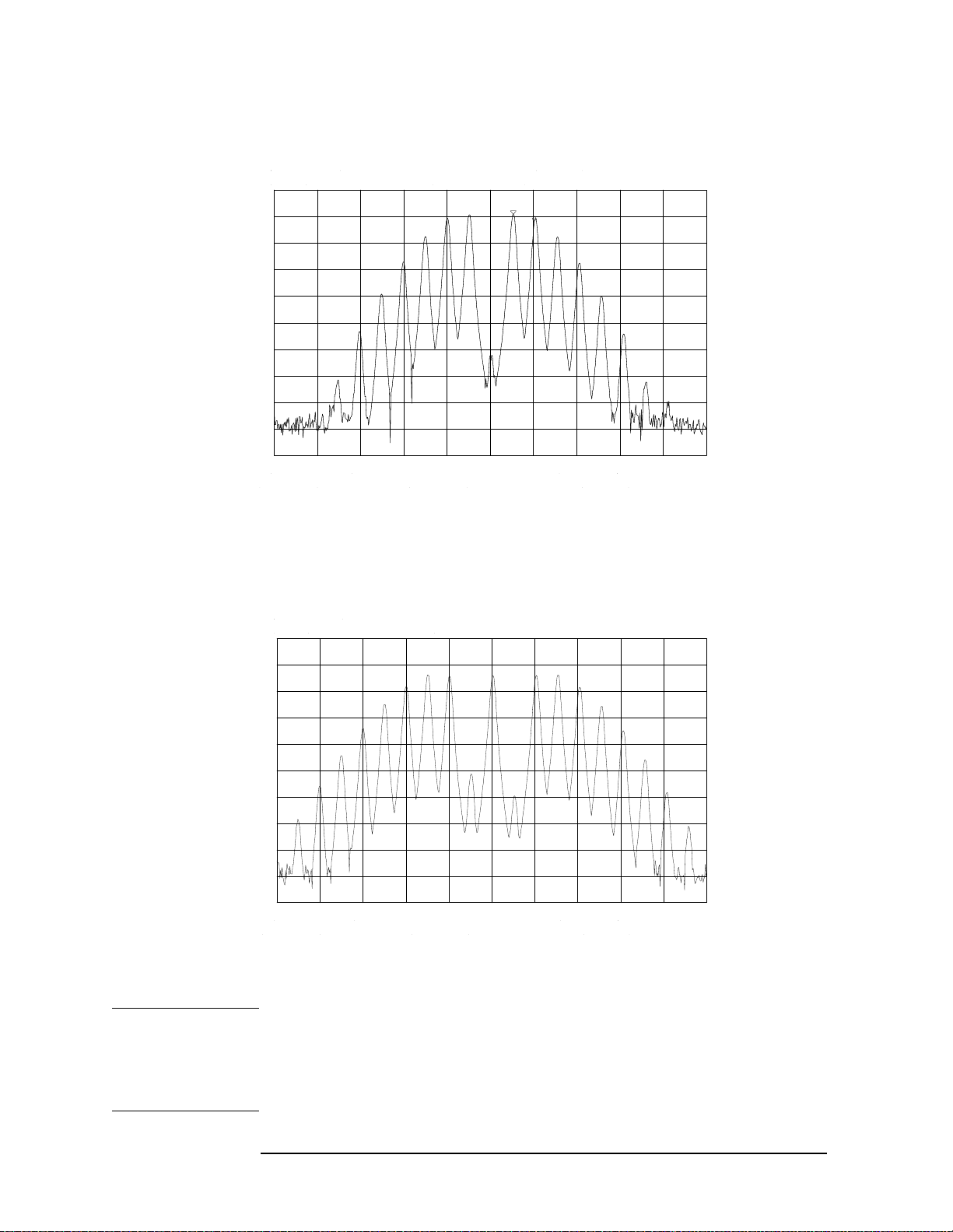
Making Measurements
Example 3: Modulation
Figure 2-13 FM Signal with Carrier at a Null
Figure 2-14 FM Signal with First Sidebands at a Null
NOTE Incidental AM from a source signal can cause the frequency null to shift, resulting in
errors to the procedure above. Incidental AM is very low for most RF signal generators,
but can be significant in microwave signal generators. Nonsymmetrical side lobes
indicate the presence of incidental AM. In such cases, the best technique for measuring
FM is to down-convert and use a modulation analyzer such as the HP 8901A/B.
64 Chapter2
Page 65

Making Measurements
Example 4: Harmonic Distortion
Example 4: Harmonic Distortion
What Is Harmonic Distortion?
Most transmitting devices and signal sources contain harmonics.
Measuring the harmonic content of such sources is frequently required.
In fact, measuring harmonic distortion is one of the most common uses
of a spectrum analyzer. Harmonic distortion can be checked very
quickly by using the measurement routine described below. This
measurement routine measures harmonic amplitudes relative to the
source frequency.
Spectrum Analyzer Functions Used
The following harmonic distortion measurement applies an important
group of spectrum analyzer operating skills: setting the frequency span
using start and stop frequencies; setting the video bandwidth; and
making relative measurements using two markers. It also
demonstrates setting a signal to center frequency using a marker, and
setting the frequency step size to the value of the center frequency.
There are two common ways to measure harmonic distortion using a
spectrum analyzer. Procedure A illustrates the faster method, which
permits a simultaneous display of the fundamental and its harmonics.
Procedure B takes longer to perform but provides a better
measurement of harmonics closer to the noise floor.
Stepping through the Fast Harmonic Measurements:
Procedure A
This example measures the harmonic content of a 1 MHz signal
provided by a signal generator. You may use the 300 MHz calibrator
signal of the spectrum analyzer, but be sure to adjust the spectrum
analyzer start and stop frequencies to accommodate the source
frequency and its harmonics.
1. Connect the signal source to the spectrum analyzer INPUT 50 Ω.
Press
Measure the 1 MHz fundamental and its first two harmonics
1. Set the start frequency to 450 kHz.
2. Set the stop frequency to 3.5 MHz.
PRESET to start the procedure from a preset state.
This displays the fundamental frequency and the second and third
harmonics as shown in Figure 2-15 on page 66.
Chapter 2 65
Page 66
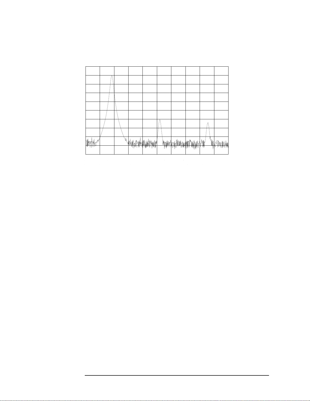
Making Measurements
Example 4: Harmonic Distortion
Figure 2-15 Input Signal and Harmonics
1. Set the video bandwidth to improve visibility by smoothing the
noise:
a. Press
b. Press
c. Use the step down
BW.
VIDEO BW AUTO MAN until MAN is selected.
⇓ key to select the video bandwidth.
2. Formeasurement accuracy, raise the peak of the fundamental to the
reference level:
a. Press
PEAK SEARCH, MKR →, MARKER → REF LVL. The result is
shown in Figure 2-16.
66 Chapter2
Page 67
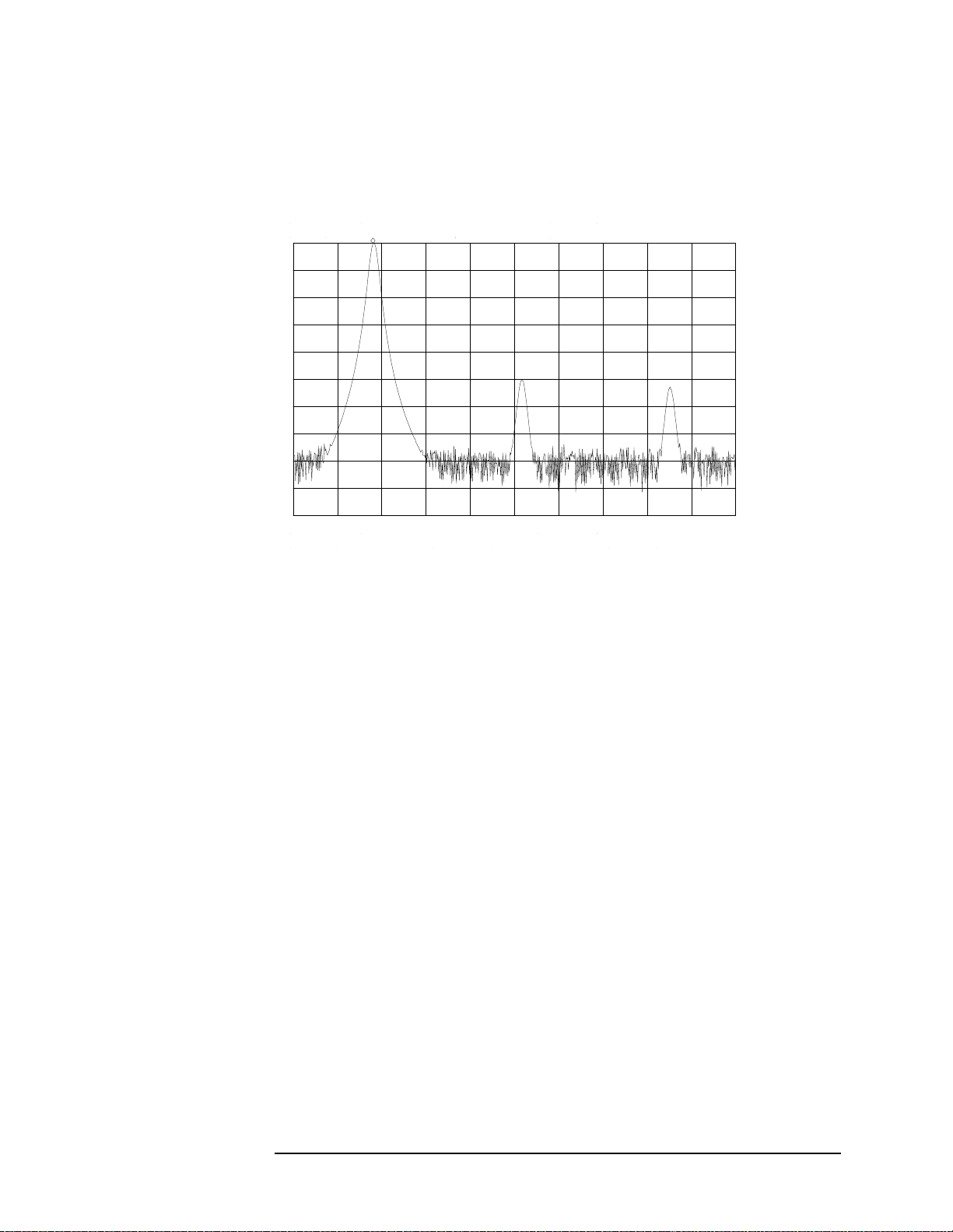
Making Measurements
Example 4: Harmonic Distortion
Figure 2-16 Peak of Signal is Positioned at Reference Level for Maximum
Accuracy
Place a second marker on the second harmonic
1. Set the peak threshold above the noise:
a. Press PEAK SEARCH, MORE 1 OF 2, PEAK THRESHLD.
b. Adjust the dashed line to a level above the noise using either the
step keys or the knob.
2. Activate the second marker:
a. Press
PEAK SEARCH, MARKER DELTA, NEXT PK RIGHT.
This places the anchor marker on the fundamental, and a second
marker on the peak of the second harmonic, as shown in Figure 2-17 on
page 68.
Chapter 2 67
Page 68
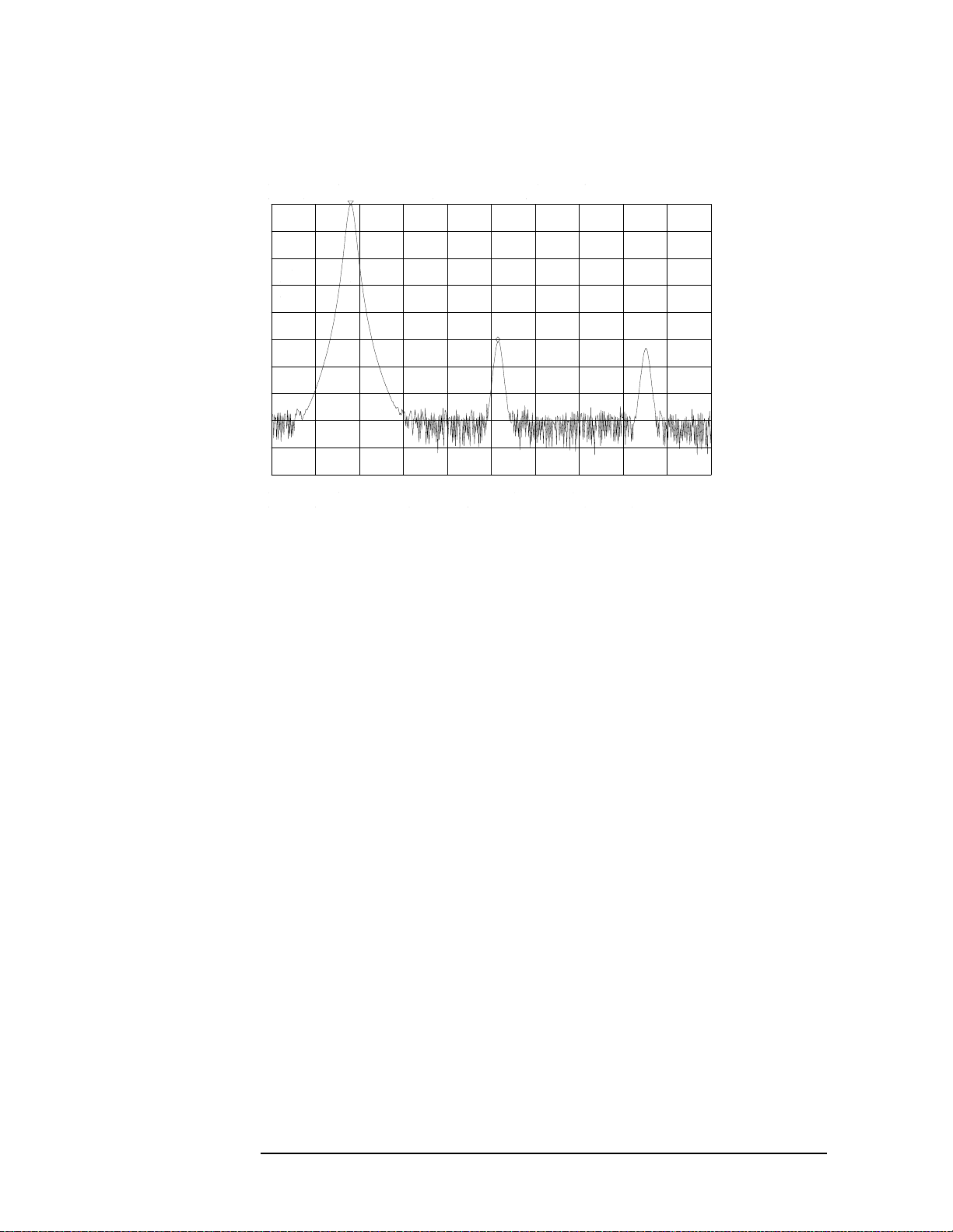
Making Measurements
Example 4: Harmonic Distortion
Figure 2-17 Harmonic Distortion in dBc (marker threshold set to −70 dB)
Find the harmonic distortion (method 1)
The difference in amplitude between the fundamental and second
harmonic shown in the figure is about −50 dB, or 0.33 percent harmonic
distortion (see Figure 2-18).
1. To measure the third harmonic, press
NEXT PK RIGHT again.
Measure additional harmonics
1. Continue reading amplitudes and comparing them to Figure 2-18 for
each additional harmonic you want to measure.
PEAK EXCURSN
defines what is and what is not a peak; the next-peak routines find
the corresponding peak.
68 Chapter2
Page 69

Making Measurements
Example 4: Harmonic Distortion
Figure 2-18 Percentage of Distortion versus Harmonic Amplitude
Find the harmonic distortion (method 2)
1. Another easy way of determining the percent of distortion is to
change the units to volts:
a. Press
AMPLITUDE, MORE 1 OF 3, AMPTD UNITS, VOLTS. The
marker readout automatically changes to voltage units.
b. To determine the percentage of distortion, use the ratio given by
the marker and move the decimal point of this value two places to
the right. However, the displayed ratio is limited to a minimum of
0.01, or 1 percent, before reaching zero.
Plot the display
1. You may want to plot the display for hard-copy documentation:
a. Connect a graphics plotter (such as an HP 7440A ColorPro) to the
analyzer via HP-IB.
b. Set the plotter address to 5.
c. On the spectrum analyzer, press
PLT until PLT is selected.
d. Press
e. Press
PLOTTER CONFIG to view available plot functions.
COPY to transfer the entire display to the plotter.
CONFIG, then COPY DEV PRNT
Other plotter functions let you select certain traces or parts of the
display for plotting. The PLOT ORG DSP GRAT function lets you choose
the plotter reference points to correlate to the display (DSP) or to the
display graticule (GRAT).
Chapter 2 69
Page 70

Making Measurements
Example 4: Harmonic Distortion
An Alternative Harmonic Measurement Method:
Procedure B
This method is somewhat longer, but because each signal is measured
in a narrower span and resolution bandwidth, the signal-to-noise ratio
is improved, making the results more accurate.
1. Using the present setup, clear the markers from the screen by
pressing
HOLD is pressed, the display expands to the full size of the screen, for
easier viewing.
Measure the 1 MHz fundamental
1. Reduce the frequency span:
MKR, MARKERS OFF. Notice that when MARKERS OFF or
a. Press
PEAK SEARCH, which activates a marker on the
highest-level signal on-screen.
b. Reduce the frequency span to 1 MHz by pressing SPAN, SPAN
ZOOM.
c. Enter 1 MHz. The span zoom function lets you quickly "zoom" to a
narrower frequency span without losing the signal from the
screen (because signal track is activated).
d. After the frequency span is reduced, turn off the signal-track
function by pressing
MKR, and setting SIG TRK ON OFF to OFF.
2. Set the center-frequency step-size to the frequency of the
fundamental:
a. Press
MKR →, MARKER → CF STEP
3. For better amplitude accuracy, move the signal to the top of the
graticule:
a. Press
MARKER → REF LVL. The resulting display should resemble
Figure 2-19 on page 71.
70 Chapter2
Page 71
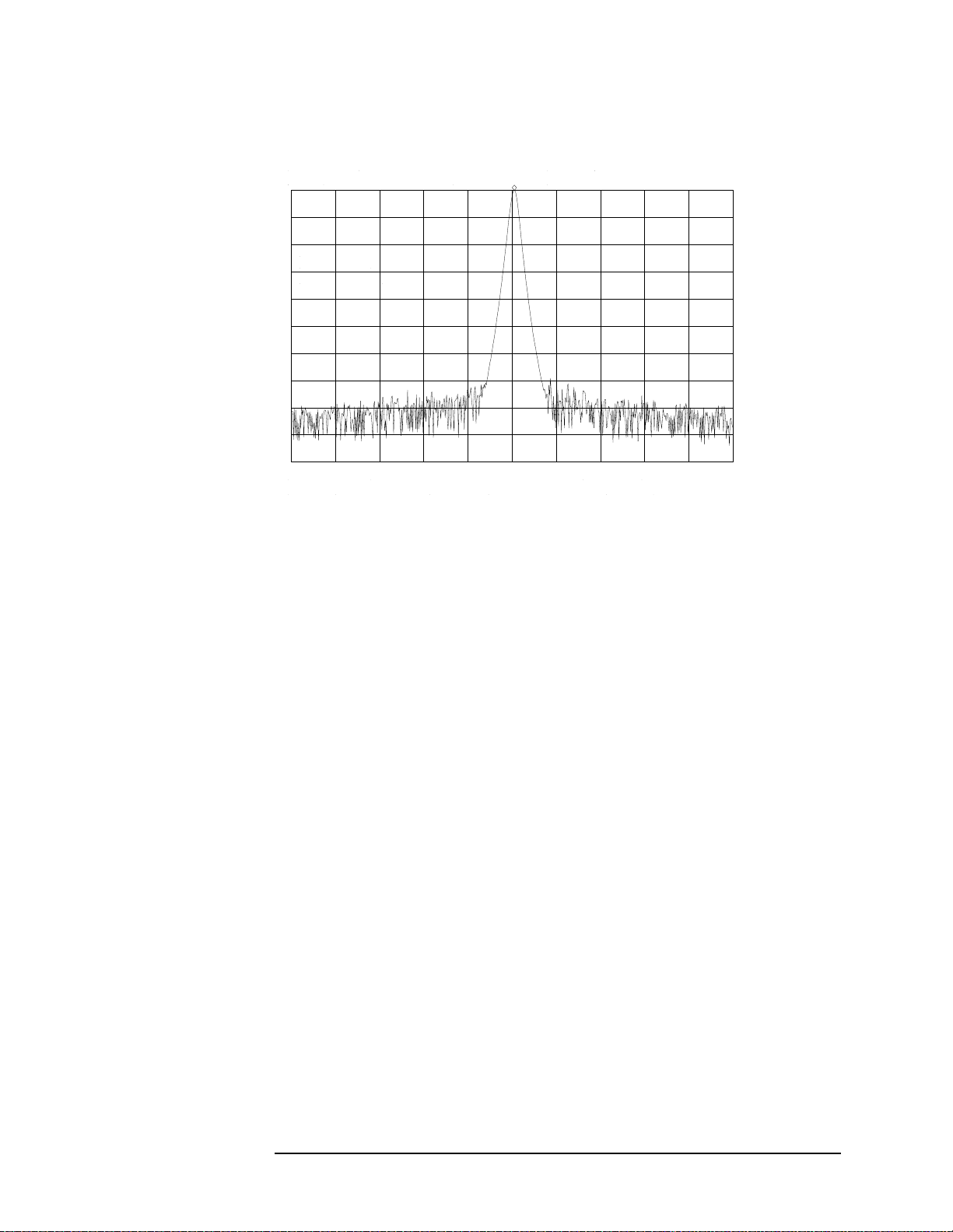
Figure 2-19 Input Signal Displayed in a 1 MHz Span
Making Measurements
Example 4: Harmonic Distortion
Measure the second harmonic
1. Press
MKR, MARKER DELTA, FREQUENCY, and the step up › key. This
step retunes the spectrum analyzer center frequency to the second
harmonic.
2. Adjust the harmonic to the reference level. (Note that the
REF LVL function is not available in marker-delta mode.) This
MARKER →
displays the amplitude of the second harmonic as shown in Figure
2-20 on page 72.
Find the harmonic distortion
1. Use Figure 2-18 on page 69 to convert the difference between the
second harmonic and the fundamental to a percentage of distortion.
Again, units can be changed to volts in order to read the voltage ratio
of the two signals.
Measure additional harmonics
1. Foreach additional harmonic you wish to measure, press the step up
› key and adjust the reference level. Note the arrow in the upper-left
corner of the graticule indicates that the anchor markerisoff-screen.
However, the results are still valid.
Chapter 2 71
Page 72
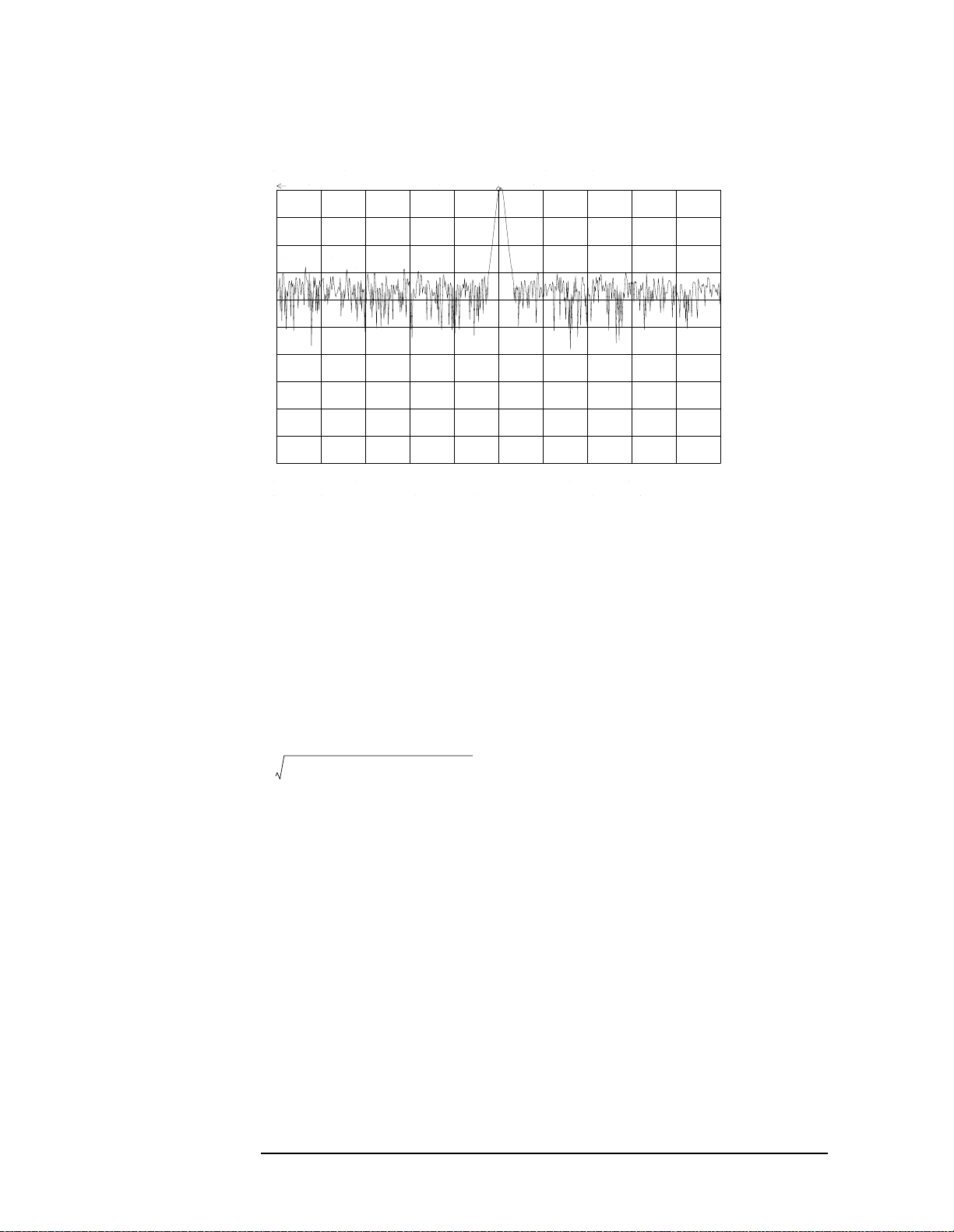
Making Measurements
Example 4: Harmonic Distortion
Figure 2-20 Second Harmonic Displayed in dBc
Percent of Harmonic Distortion
The total percent of harmonic distortion of a signal is also measured
frequently. For this measurement, the amplitude of each harmonic
must be measured in linear units (for example, volts) instead of dBc. To
display amplitude units in volts, press
AMPTD UNITS, and VOLTS. The amplitude values of these signals are
used in the equation below to compute total harmonic distortion:
A2()2A3()2A4()2.... An()
+ + + 100×
----------------------------------------------------------------------------------------------------
A
1
2
1. Where:
= the amplitude of the fundamental frequency, in volts
A
1
A
= the amplitude of the second harmonic, in volts
2
A
= the amplitude of the third harmonic, in volts
3
A
= the amplitude of the fourth harmonic, in volts
4
A
= the amplitude of the nth harmonic, in volts
n
If the signal amplitudes are measured carefully, as in the previous
example, this procedure measures percent-of-harmonic distortion very
accurately.
AMPLITUDE, MORE 1 OF 3,
72 Chapter2
Page 73

Making Measurements
Example 5: Third-Order Intermodulation Distortion
Example 5: Third-Order Intermodulation
Distortion
What Is Intermodulation Distortion?
In crowded communication systems, signal interference of one device
with another is a common problem. For example, two-tone, third-order
intermodulation often is a problem in narrow-band systems. When two
signals (F
second-order harmonics that are generated (2F
third-order intermodulation distortion products,which are located close
to the original signals at 2F
intermodulation distortion can also occur. These distortion products are
generated by such system components as amplifiers and mixers.
Spectrum Analyzer Functions Used
and F2) are present in a system, they can mix with the
1
and 2F2), creating
1
and 2F1−F2. Higher order
2−F1
The following procedure describes how to measure third-order
intermodulation distortion. It shows how to tune two signals onto the
spectrum analyzer display and demonstrates setting the resolution
bandwidth, mixer level, and reference level. It also incorporates several
marker functions.
Stepping through the Measurement
Set up the test
1. To test a device for third-order intermodulation, connect the
equipment as shown in Figure 2-21 on page 74. This example uses a
6 dB directional coupler, and two sources set to 20 MHz and 21 MHz.
You may substitute other source frequencies, but for this example,
maintain a frequency separation of about 1 MHz. The device under
test is a 26 dB preamplifier. The low-pass filters are required to stop
the signal from the two sources from causing distortion due to
reflecting the signal. If you are performing this procedure only for
practice using the instrument, you don't need the low-pass filters.
Chapter 2 73
Page 74

Making Measurements
Example 5: Third-Order Intermodulation Distortion
Figure 2-21 Third-Order Intermodulation Test Setup
2. Set one source to 20 MHz and the other source to 21 MHz, for a
frequency separation of 1 MHz.
3. Set the sources equal in amplitude (for this example, we have set the
sources to −30 dBm).
Reduce the frequency span
4. Tune both signals onto the display by setting the center frequency to
20.5 MHz.
5. Reduce the frequency span to 5 MHz for a span wide enough to
include the distortion products on the display. For frequency
separations other than those used in this example, choose a span
greater than three times the separation of the source signals.
NOTE A quick way to get to a smaller frequency span is to use SPAN ZOOM.
SPAN ZOOM activates a highest-peak marker, turns signal track on, and
zooms down to the span selected by the user.
To activate the span zoom function, press SPAN, SPAN ZOOM, and enter
5 MHz. Be sure to turn signal track off before changing other spectrum
analyzer settings.
Center and adjust the signals on the display
6. Press
FREQUENCY.
7. Using the knob, center the two signals on the display, as shown in
Figure 2-22 on page 75.
8. To resolve the distortion products, reduce the resolution bandwidth
until the distortion products are visible:
74 Chapter2
Page 75

a. Press BW.
Making Measurements
Example 5: Third-Order Intermodulation Distortion
b. Use the step down
⇓ key to reduce the resolution bandwidth.
9. Reduce the video bandwidth, if necessary.
10.To make sure the input signals are equal in amplitude:
a. Press
PEAK SEARCH, MARKER DELTA, and NEXT PEAK.
b. Adjust the signal source with the corresponding marker on it
until the difference in amplitude reads zero.
NOTE If you need to choose a specific resolution bandwidth to verify that the
distortion products are at a certain level below the source signal, refer
to Example 1 in this chapter.
Figure 2-22 Signals Centered on Spectrum Analyzer Display
Set the reference level
11.Forgreatest measurement accuracy, position the peaks of the source
signals at the reference level. The spectrum analyzer function
MARKER → REF LVL lets you set the reference level using a marker:
a. Place a marker on the source signal of highest amplitude by
pressing
b. Set the reference level to this value by pressing
MARKER → REF LVL. Figure 2-23 on page 76 illustrates the
PEAK SEARCH, MARKER NORMAL.
MKR →,
resulting display.
Chapter 2 75
Page 76

Making Measurements
Example 5: Third-Order Intermodulation Distortion
Figure 2-23 Signal Peak Set to Reference Level
Maximize dynamic range
12.Distortion-free dynamic range is important for this type of
measurement. To maximize such dynamic range:
a. Set the mixer input level to −30 dBm by pressing
MORE 1 OF 3, MAX MXR LEVEL.
AMPLITUDE,
b. Enter −30 dBm.
The spectrum analyzer automatically sets the attenuation so the
maximum signal level is −30 dBm at the input mixer when the signal is
at or below the reference level (see Example 1). You will hear the input
attenuator click; notice that the value of the attenuator is now 20 dB
(see Figure 2-24 on page 77).
This change to the maximum mixer level can affect the noise, so you
may need to adjustment the resolution and video bandwidths.
Set a second marker and measure the distortion product
Once a marker is activated, the marker delta function activates a
second marker and displays the difference between the two markers.
Relative measurements can then be performed easily.
13.To measure a distortion product:
a. Press
b. To activate a second marker, press
76 Chapter2
PEAK SEARCH to place a marker on a source signal.
MARKER DELTA.
Page 77

Example 5: Third-Order Intermodulation Distortion
c. Press NEXT PK LEFT or NEXT PK RIGHT to set the second marker
on the peak of the distortion product that is beside the signal
source (see Figure 2-24).
The difference in frequency and amplitude between the two markers is
displayed in the active function block.
Figure 2-24 Intermodulation Distortion Measured in dBc
Making Measurements
Create a title for the measurement
The screen title function lets you create a title on the screen, and a label
for the recall menu.
14.To create a title:
a. Press
DISPLAY, SCREEN TITLE.
b. Use the softkeys from the screen-title menu and the knob (to
choose the letters) to create a title. The title appears in the
upper-right corner of the graticule; it can be up to two rows of 16
characters each (see Figure 2-25).
c. Press
TITLE DONE when the title is complete.
Chapter 2 77
Page 78

Making Measurements
Example 5: Third-Order Intermodulation Distortion
Figure 2-25 Display with Title
Save the measurement information
The save and recall functions allow you to store data for later viewing.
15.To save the instrument state:
a. Press
SAVE, SAVE STATE.
b. Press a softkey to enter the instrument state data into the
register (0 to 9) you select. The first 16 characters of the title are
used to label the register on the recall menu.
16.To view this menu, press RECALL, RECALL STATE. If a stored state
has not been titled, the menu reads STATE followed by the register
number chosen.
78 Chapter2
Page 79

Making Measurements
Example 6: AM and FM Demodulation
Example 6: AM and FM Demodulation
What is AM and FM Demodulation?
Amplitude modulation (AM) and frequency modulation (FM) are
common modulation techniques used to broadcast information. In the
United States and Canada, the AM broadcast band is 535 kHz to 1605
kHz, while the FM broadcast band covers 88 MHz to 108 MHz.
Demodulation of AM and FM signals can be done with any spectrum
analyzer with zero span capability and with a wide enough bandwidth
to fully encompass the modulated signal. An easier method of
examining a demodulated signal is to use the built-in AM and FM
demodulator and speaker in the HP 8560 E-Series and EC-Series
spectrum analyzers.
Forsimplicity, in our example we will demodulate only an FM signal. To
demodulate and listen to an AM signal, repeat the same steps, but
activate
AM DEMOD ON OFF instead of FM DEMOD ON OFF.
Spectrum Analyzer Functions Used
The following procedure illustrates the use of the built-in AM and FM
demodulator and speaker. The example includes tuning the spectrum
analyzer to a band of interest, activating and moving a marker to the
signal that is to be demodulated, and demodulating and listening to the
signal with the built-in demodulator and speaker.
Stepping through the Measurement
Set up the test
1. Provide a signal to the spectrum analyzer by connecting an antenna
to the input port of the spectrum analyzer.
Chapter 2 79
Page 80
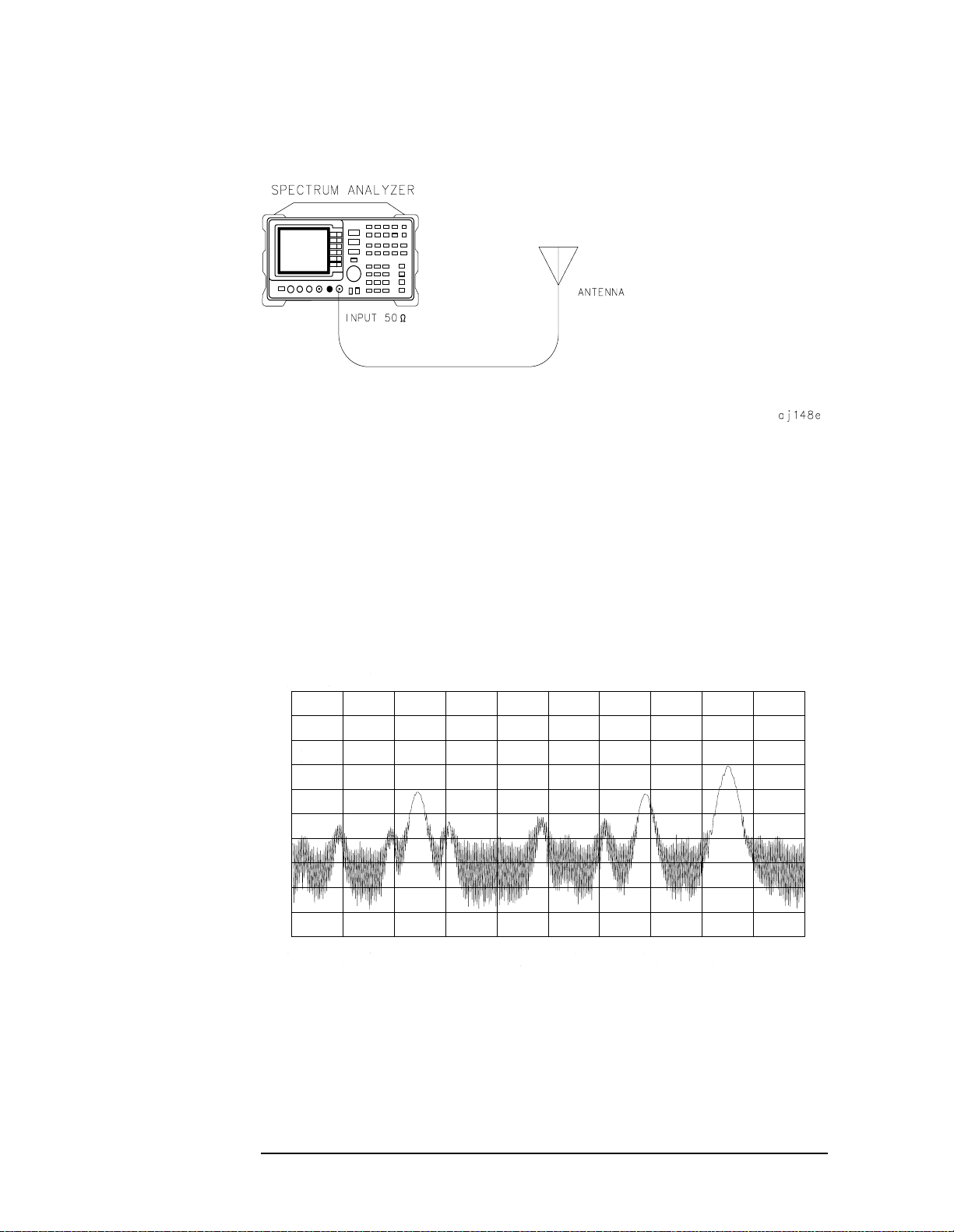
Making Measurements
Example 6: AM and FM Demodulation
Figure 2-26 AM and FM Demodulation Test Setup
Set the start and stop frequencies
2. Tune to the FM band by setting the start frequency of the spectrum
analyzer to 88 MHz, and the stop frequency to 108 MHz:
a. Press
b. Press
c. Press
Figure 2-27 FM Band
FREQUENCY.
START FREQ; enter 88 MHz.
STOP FREQ; enter 108 MHz (see Figure 2-27).
Set a marker
3. Todemodulate an FM signal, you must activate a marker before you
turn on the demodulator. For your convenience, the AM and FM
demodulation menu contains the marker functions.
80 Chapter2
Page 81
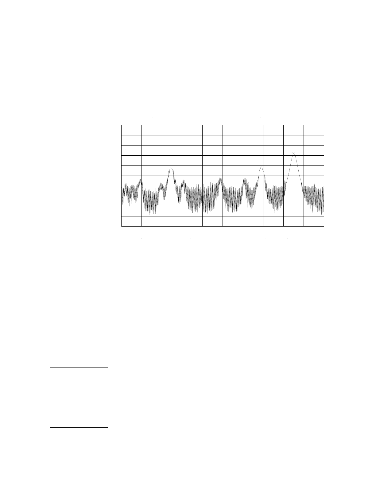
Making Measurements
Example 6: AM and FM Demodulation
a. Press AUX CTRL AM/FM DEMOD to access the demodulation menu.
b. Activate a marker by pressing
MARKER NORMAL.
c. Position the marker on the signal of interest. If the signal of
interest is the highest in amplitude, press PEAK SEARCH directly,
as in Figure 2-28 on page 81.
Figure 2-28 Place a marker on the signal of interest, then demodulate.
Set the time
4. For this example, before demodulating the signal, set the
demodulation time to 30 seconds:
a. pressing
MORE 1 OF 2, DEMOD TIME.
b. Enter 30 seconds. This sets the actual time that the built-in
demodulator will demodulate the signals so you may listen to it.
Demodulate the signal
5. Press
MORE 2 OF 2, then set FM DEMOD ON OFF to ON.Youmay have
to adjust the volume of the speaker using the volume knob located on
the front panel, under the display.
NOTE You also can use AM or FM demodulation when the frequency span of
the spectrum analyzer is zero. To obtain continuous demodulation in
zero span, set the trigger mode to external by pressing
EXTERNAL. Setting the spectrum analyzer to the external trigger mode
TRIG,
(without actually supplying a trigger) gives you an uninterrupted
signal. Otherwise, demodulation will occur only during the spectrum
analyzer sweep.
Chapter 2 81
Page 82
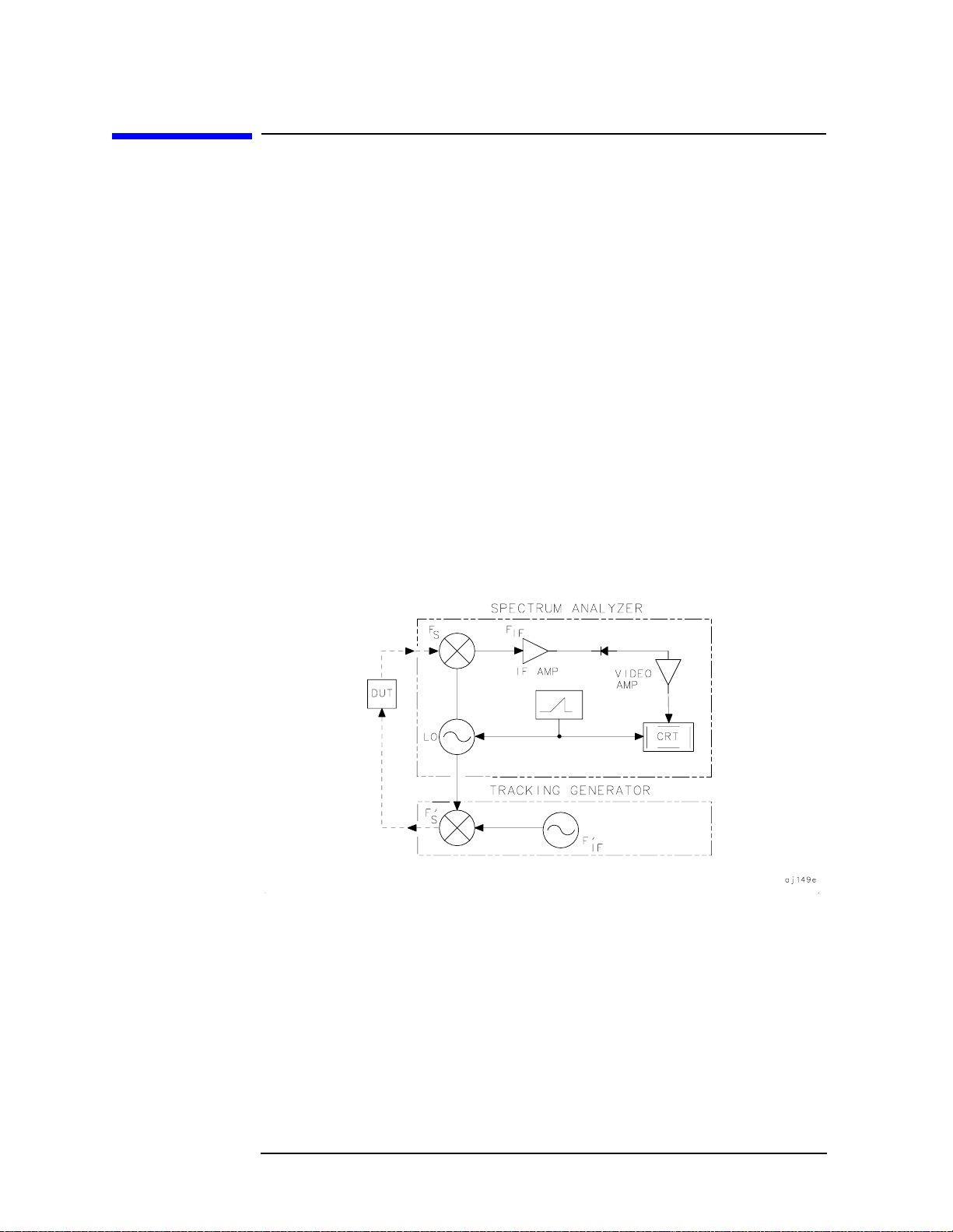
Making Measurements
Example 7: Stimulus-Response Measurements
Example 7: Stimulus-Response Measurements
What Are Stimulus-Response Measurements?
Stimulus-response measurements require a source to stimulate a
device under test (DUT), and a receiver to analyze the
frequency-response characteristics of the DUT. Characterization of a
DUT can be made in terms of its transmission or reflection parameters.
Ripple, flatness, and rejection are examples of transmission
measurements. A typical reflection measurement is return loss.
A spectrum analyzer combined with a tracking generator forms a
stimulus-response measurement system. With the tracking generator
as the swept source and the spectrum analyzer as the receiver,
operation is analogous to a single-channel scalar network analyzer.
Because the tracking generator is a narrow-band system, its output
frequency must be made to track the spectrum analyzer input
frequency precisely, resulting in a wide dynamic range. This wide
dynamic range will be illustrated in the following example.
Figure 2-29 Block Diagram of a Spectrum Analyzer and Tracking Generator
System
Spectrum Analyzer Functions Used
The following procedure describes how to use the HP 8560E/EC Option
002 spectrum analyzer with built-in tracking generator system to
measure the rejection range of a bandpass filter, which is a type of
transmission measurement. The same measurement can be made using
an HP 8560E/EC (without Option 002), HP 8561E/EC, HP 8562E/EC,
HP 8563E/EC, HP 8564E/EC or HP 8565E/EC spectrum analyzer with
an HP 85640A, HP 85644A, or HP 85645A tracking generator. This
82 Chapter2
Page 83
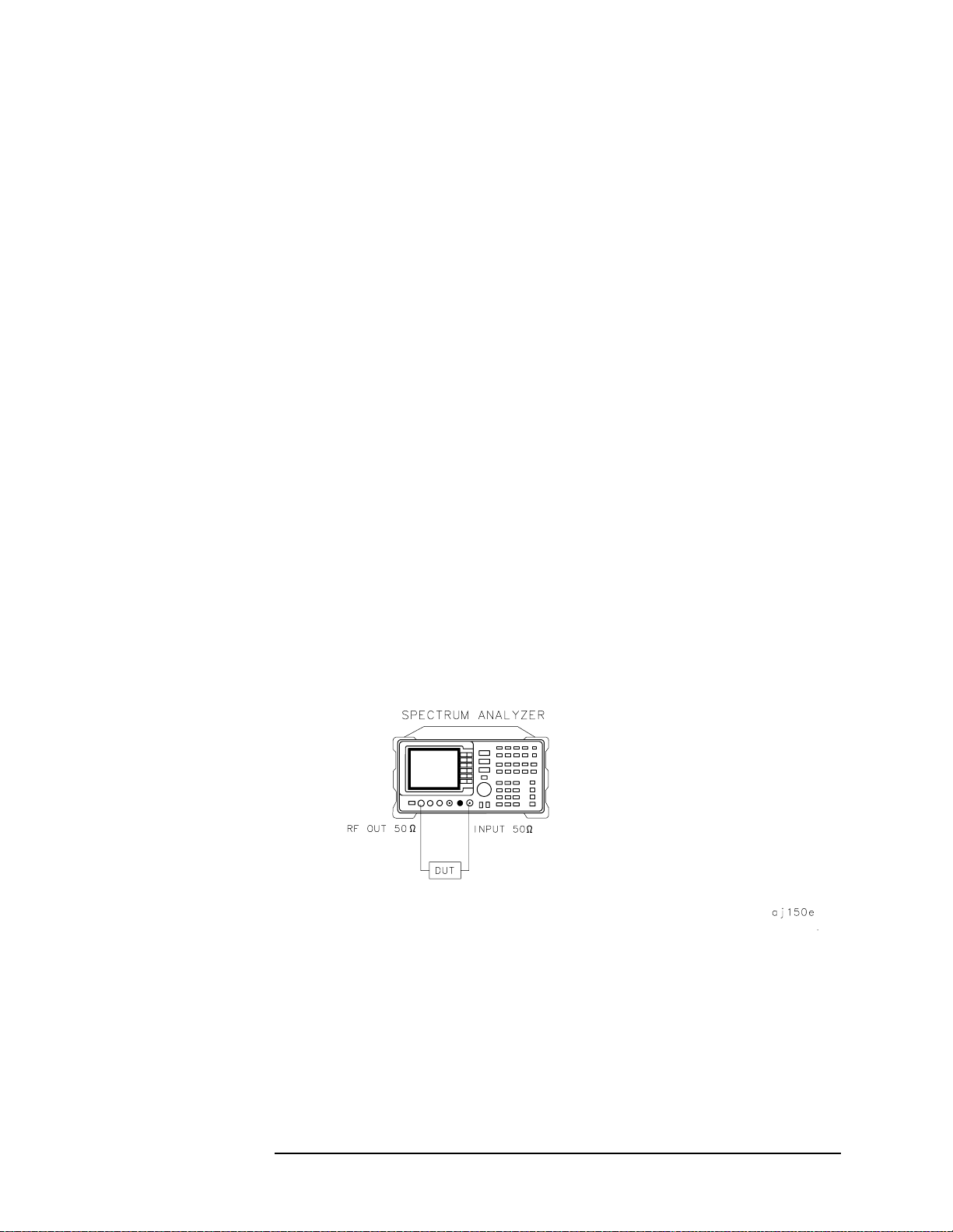
Making Measurements
Example 7: Stimulus-Response Measurements
example illustrates several functions in the HP 8560E/EC Option 002
tracking-generator menu: adjusting the tracking-generator output
power, source calibration, and normalization.
Because the procedure for conducting a reflection measurement is
similar, use this example as your guide. You may also refer to the
HP Spectrum Analyzer Seminar, Application Note 150-7, or
Applicaton Note 1212 for more information about reflection
measurements.
Stepping through the Measurement
There are four basic steps for performing any stimulus-response
measurement (either transmission or reflection):
1. Set up the spectrum analyzer settings
2. Calibrate
3. Normalize
4. Measure
Set up the test
1. To measure the rejection of a bandpass filter, connect the equipment
as shown in Figure 2-30. This example uses a bandpass filter with a
center frequency of 321.4 MHz and a specified rejection of −85 dB, as
the device under test (DUT).
Figure 2-30 Transmission Measurement Test Setup
Set the spectrum analyzer
2. To activate the tracking generator menu, press
TRACKING GENRATOR. The tracking-generator output power is
AUX CTRL,
displayed in the active function block. Because the filter (DUT) is not
particularly sensitive, an output power of −10 dBm should not
damage it.
Chapter 2 83
Page 84
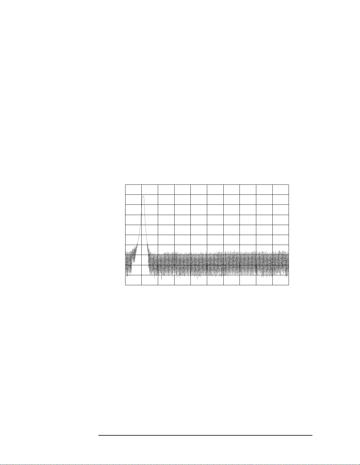
Making Measurements
Example 7: Stimulus-Response Measurements
3. Activate the tracking-generator power level by pressingSRC PWR ON
OFF until ON is selected.
If ERR 901 TGFrqLmt appears in the error message area, set the
start frequency to 300 kHz.(Stimulus-response measurements using
an HP 8560E/EC Option 002 are specified from 300 kHz to 2.9 Ghz.)
Due to the current resolution of the annotation, changing the start
frequency to 300 kHz will be denoted only in smaller spans.
4. Put the sweep time of the analyzer into stimulus-response
auto-coupled mode by pressing
MORE 1 OF 3, then SWP CPL SR SA
until SR is selected. In stimulus-response mode, the auto-coupled
sweep times usually are much faster for swept-response
measurements (see Figure 2-31).
Figure 2-31 Tracking-Generator Output Power Activated
5. Because we are interested only in bandpass-filter rejection, tune the
center frequency so the filter roll off takes up most of the trace on the
display (see Figure 2-32).
84 Chapter2
Page 85
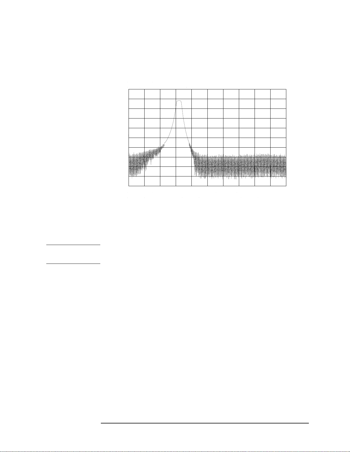
Making Measurements
Example 7: Stimulus-Response Measurements
Figure 2-32 Adjust analyzer settings according to the measurement
requirement.
6. Decrease the resolution bandwidth to increase sensitivity, and
narrow the video bandwidth to smooth the noise. In Figure 2-33, the
resolution bandwidth has been decreased to 3 kHz.
NOTE The minimum resolution bandwidth supported in stimulus-response
measurements is 300 Hz.
Chapter 2 85
Page 86
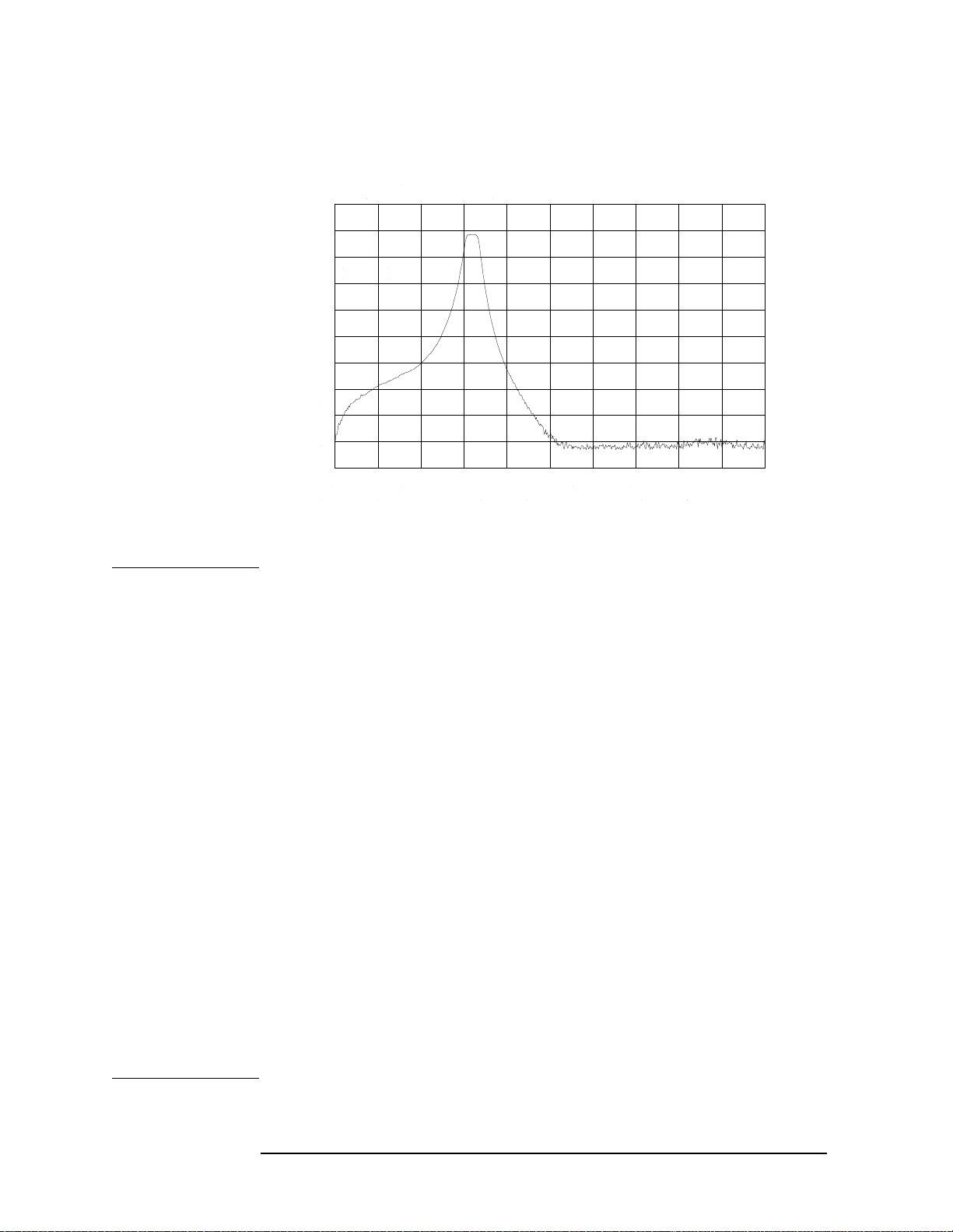
Making Measurements
Example 7: Stimulus-Response Measurements
Figure 2-33 Decrease the resolution bandwidth to improve sensitivity.
NOTE Tracking Error
Adjusting the resolution bandwidth may result in a decrease in
amplitude of the signal. This is known as a tracking error. Tracking
errors occur when the tracking generator output frequency does not
exactly match the input frequency of the spectrum analyzer. The
resulting product from the spectrum analyzer input mixer is not at the
center of the IF bandwidth. Tracking errors are most notable when
using narrow resolution bandwidths.
Compensate for the tracking error, by using either the manual or the
automatic tracking adjustment. These keys are on the second softkey
menu page of
TRACKING GENRATOR under the AUX CTRL key.
Automatic Tracking
Once the automatic tracking routine is activated in a wide resolution
bandwidth, it is not necessary to use the tracking adjust again when
decreasing the resolution bandwidth. The automatic tracking routine
uses the 300 Hz resolution bandwidth to perform the tracking
adjustment.
Toactivate the automatic tracking routine, press
press
MAN TRK ADJ to display the DAC values of the coarse- and
fine-tracking adjustments. In this example, the automatic tracking
routine was performed, and the resolution bandwidth was decreased to
300 Hz, without encountering any tracking error (see Figure 2-34).
TRACKING PEAK, then
86 Chapter2
Page 87
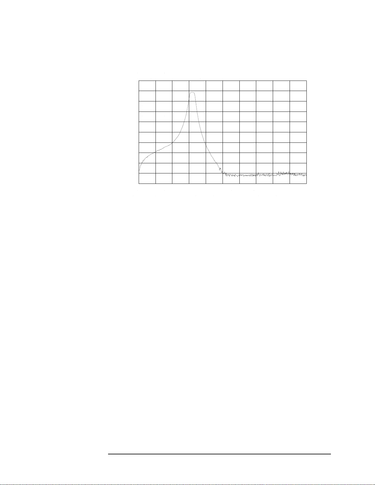
Making Measurements
Example 7: Stimulus-Response Measurements
Figure 2-34 Manual tracking adjustment compensates for tracking error.
Calibrate
Calibration in a transmission measurement is done using a through
(thru). A thru essentially is a conductor that is connected in place of the
device under test.
7. To calibrate using a thru:
a. Press
THRU.
AUX CTRL, TRACKING GENRATOR, SOURCE CAL MENU, CAL
b. The guided calibration routine prompts you to connect the thru,
as illustrated in Figure 2-35. Connect the thru, then press STORE
THRU to store the thru trace in trace B and in an internal memory
location in the analyzer.
The state information of the thru-calibration trace is stored in
state register number 9. This trace can be recalled for future use.
Figure 2-36 shows what appears on-screen after the thru trace is
stored.
Chapter 2 87
Page 88

Making Measurements
Example 7: Stimulus-Response Measurements
Figure 2-35 Guided calibration routines prompt the user.
Figure 2-36 The thru trace is displayed in trace B.
Normalize
Normalization eliminates the frequency response error in the test
setup. When normalization is on, trace math is performed on the active
trace:
A − B + NRP → A
1. where:
A is the active trace.
B is the stored thru calibration trace.
NRP is the normalized reference position.
88 Chapter2
Page 89
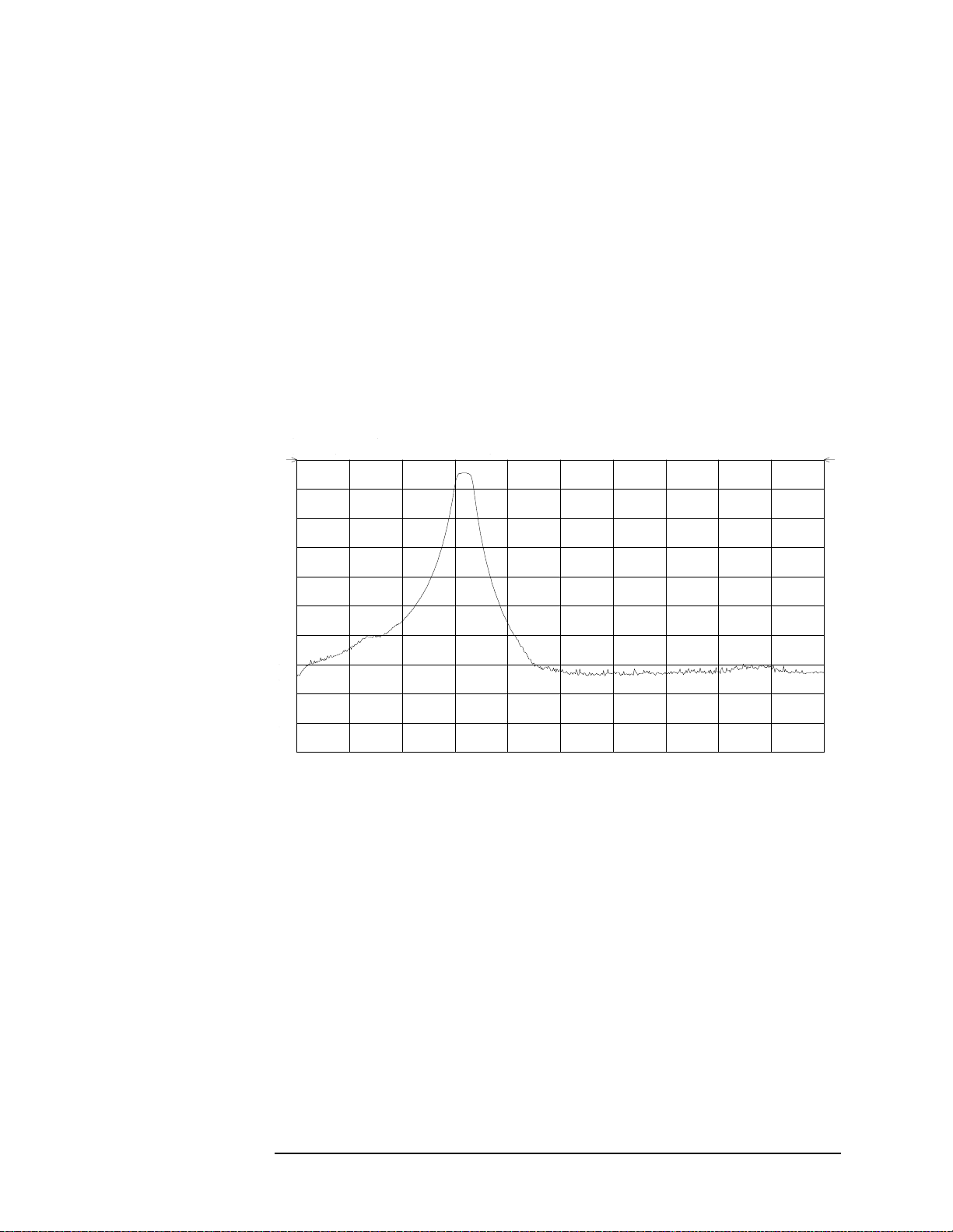
Making Measurements
Example 7: Stimulus-Response Measurements
The units of the reference level, dB, reflect this relative measurement
(see Figure 2-37).
• To normalize, press
softkey is located on the first page of the tracking-generator menu.)
An arrow appears on each side of the graticule when normalization is
activated. These two arrows mark the normalized reference position, or
the position where 0 dB insertion loss (transmission measurements) or
0 dB return loss (reflection measurements) will normally reside.
You can set the dB value of the normalized reference position using the
NORM REF LVL adjustment under the AMPLITUDE key. Changing
NORM REF POSN changes the position of the normalized trace, within
the range of the graticule.
Figure 2-37 Normalized Trace
NORMLIZE ON OFF until ON is selected. (This
Measure
Measure the range using the delta markers:
1. Press
PEAK SEARCH, MARKER DELTA.
2. Use the knob to position the second marker in the rejection area of
the bandpass filter as shown in Figure 2-38.
Chapter 2 89
Page 90

Making Measurements
Example 7: Stimulus-Response Measurements
Figure 2-38 Measure the rejection range with delta markers.
Activating normalization changes the softkeys that appear in the
amplitude menu:
REF LVL. Although both these functions reposition the trace on the
display,
RANGE LVL adjusts attenuation and gain, while NORM REF LVL
RANGE LVL appears, and REF LVL is replaced by NORM
does not change the spectrum analyzer settings.
NORM REF LVL, like NORM REF POSN, is a trace math function that lets
you change the position of the normalized trace within the range of the
graticule, without changing spectrum analyzer settings. See Figure
2-39. As a result, your measurement remains calibrated. However,
using these two trace math functions may mean that the top of the
screen does not represent the gain-compression limit.
90 Chapter2
Page 91

Making Measurements
Example 7: Stimulus-Response Measurements
Figure 2-39 NORM REF LVL adjusts the trace without changing analyzer
settings.
RANGE LVL increases the dynamic range of the measurement by
changing the input attenuator and IF gain. It is equivalent to
REF LVL
used in signal analysis measurements. Both RANGE LVL and REF LVL
ensure that the input signal is not in gain compression.
To increase the dynamic range of the measurement, press
RANGE LVL.
Note that while increasing the dynamic range, more errors are
introduced into the measurement, such as attenuator switching.
However, as Figure 2-40 shows, the dynamic range level has increased
by 18 dB, when using
RANGE LVL.
Chapter 2 91
Page 92

Making Measurements
Example 7: Stimulus-Response Measurements
Figure 2-40 Increase the dynamic measurement range by using RANGE LVL.
If the actual measured signal is beyond the gain-compression limit, or
below the bottom graticule of the display, an error message will appear
in the lower right corner of the display. In the case shown here, the
passband information is adjusted off-screen in order to view the
rejection range with better resolution. Changing the analyzer settings
to raise the passband information above the top of the screen results in
an ERR 903
A>DLMT.
In normalized mode, ERR 904 B>DLMT also may appear if:
• The calibration trace is off-screen, or
• No calibration has been performed after a preset, or
• Trace B is blank.
To clear this error and ensure a calibrated measurement, recalibrate
and perform a store-thru operation.
92 Chapter2
Page 93

Making Measurements
Example 7: Stimulus-Response Measurements
Using Range Level versus Using Normalized Reference Level
The following example illustrates the difference between
RANGE LVL
and NORM REF LVL. The normalized frequency response of a
preamplifier is shown in Figure 2-41. The normalized trace is cut off at
the top of the graticule. This is confirmed by the step up
⇓ key when a
marker is activated, and the ERR 903 A>DLMT error message appears in
the error message block.
Figure 2-41 Normalized Frequency Response Trace of a Preamplifier
By increasing
NORM REF LVL to 30 dB, as shown in Figure 2-42, the
trace moves down on the screen. Note that (1) the input attenuator
value remains at 10 dB, (2) the marker-amplitude readout displays 13.2
dB, and (3) the ERR 903 A>DLMT error message is still displayed, even
though the signal appears to be fully within the graticule.
Chapter 2 93
Page 94

Making Measurements
Example 7: Stimulus-Response Measurements
Figure 2-42 NORM REF LVL is a trace function.
Figure 2-43
After returning
NORM REF LVL to 0 dB, increase RANGE LVL to 30 dB. As
shown in Figure 2-43, the trace moves fully within the graticule.
Compare the settings: (1) input attenuator value has changed to 40 dB,
(2) the marker-amplitudereadout displays −6.3 dB,and (3) the ERR 903
A>DLMT error message no longer appears.
RANGE LVLadjusts analyzer for compression-free measurements.
94 Chapter2
Page 95

Making Measurements
Example 7: Stimulus-Response Measurements
Figure 2-42 shows that NORM REF LVL is a trace function that can
position the active trace without changing analyzer settings. The ERR
903 A>DLMT error message is an indicator that the actual measured
trace may fall outside of the analyzer measurement range with the
current settings. Compression-free measurements are assured by
adjusting
RANGE LVL and changing the input attenuator and IF gain.
Chapter 2 95
Page 96

Making Measurements
Example 8: External Millimeter Mixers (Unpreselected)
Example 8: External Millimeter Mixers
(Unpreselected)
External millimeter mixers can be used to extend the frequency
coverage of the HP 8560 E-Series and EC-Series spectrum analyzers.
(The HP 8560E/EC Option 002 and Option 327 do not have external
mixing capability.) Hewlett-Packardmanufactures external mixers that
do not require biasing and cover frequency ranges from 18 GHz to 110
GHz. Other manufacturers sell mixers that extend the range to 325
GHz, but may require biasing. The HP 8560 E-Series and EC-Series
spectrum analyzers support both types of mixers.
Spectrum Analyzer Functions Used
The HP 8560 E-Series and EC-Series spectrum analyzers contain an
extensive menu of functions that help with millimeter measurements.
This example explains how to connect external mixers to the spectrum
analyzer, how to choose the band of interest, how to store
conversion-loss factors, and how to use the optional automatic
signal-identification functions.
Stepping through the Measurement
Set up the equipment
1. Figure 2-44 illustrates how to connect an external harmonic mixer to
the spectrum analyzer.
CAUTION The spectrum analyzer local-oscillator output power is +16.5 dBm. Be
sure that your external harmonic mixer can accommodate this power
level before connecting it to the analyzer.
96 Chapter2
Page 97
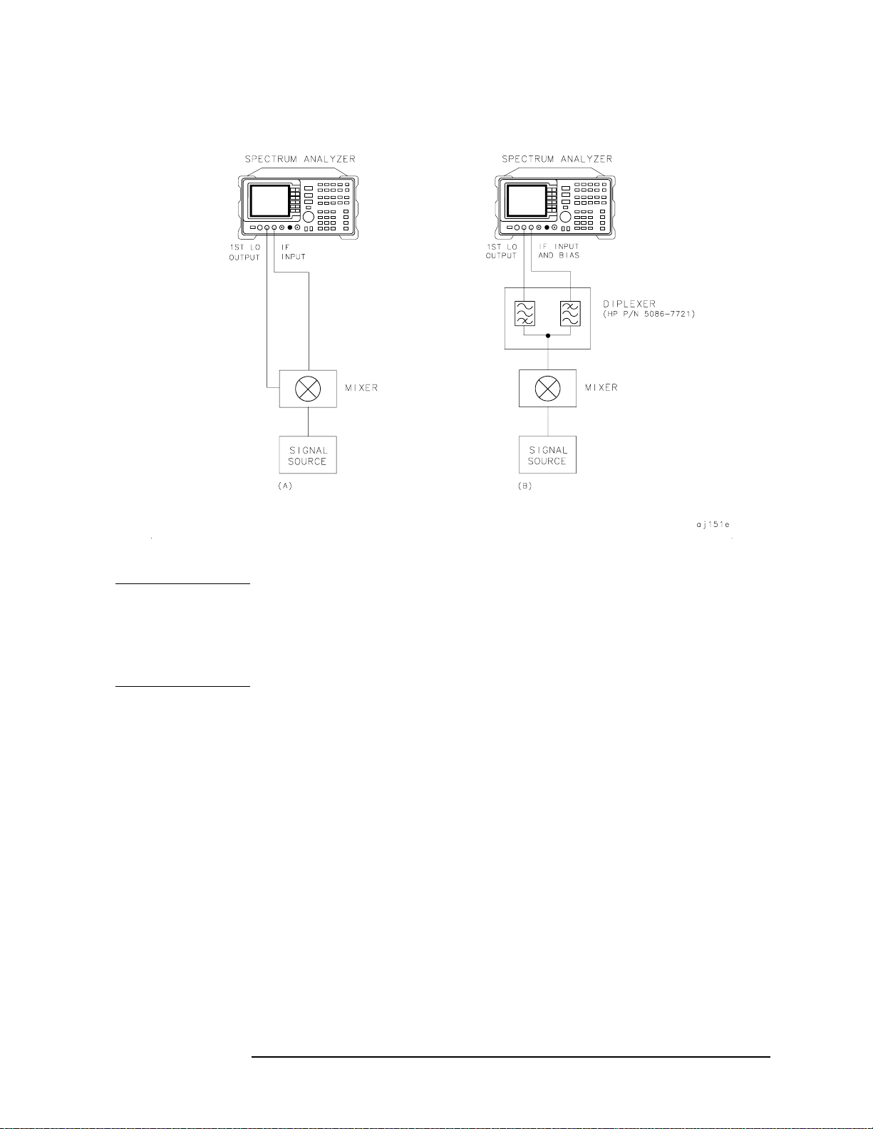
Making Measurements
Example 8: External Millimeter Mixers (Unpreselected)
Figure 2-44 External Mixer Setup (a) without Bias; (b) with Bias
NOTE Good-quality shielded SMA-type cables should be used to connect the
mixer to the spectrum analyzer to ensure that no signal attenuation
occurs. HP 5061-5458 SMA-type cables may be used. Do not
over-tighten the cables; the maximum torque should not exceed 112
N-cm (10 in-lb).
Select the Frequency Band
2. Specify unpreselected external mixing by pressing
MXR PRE UNPR until UNPR is selected.
CONFIG, then EXT
3. To select a frequency above 18 GHz:
a. Press
AUX CTRL, EXTERNAL MIXER to set the analyzer to external
mixer mode.
b. Enter the desired frequency directly using the center-frequency
function.
c. Notice in Table that some frequencies overlap and fall into two
bands. Tobe sure that the desired band is selected, refer to Table
and select the desired frequency band, then use the full band
function to enter this band.
Chapter 2 97
Page 98

Making Measurements
Example 8: External Millimeter Mixers (Unpreselected)
d. In the external mixer menu, press FULL BAND, then press the
step up
› key until the letter preceding BAND in the active function
area corresponds to the desired frequency band.
In this example, we'll look at U-band, which ranges from 40 GHz to 60
GHz, as shown in Figure 2-45. The
LOCK HARMONIC function "locks"
the spectrum analyzer in that band, ensuring that the spectrum
analyzer sweeps only the chosen band.
set to ON when
FULL BAND is pressed.
LOCK ON OFF is automatically
Table 2-4 External Mixer Frequency Ranges
Frequency
Band
K 18.0 to 26.5 6− 30 dB
A 26.5 to 40.0 8− 30 dB
Q 33.0 to 50.0 10− 30 dB
U 40.0 to 60.0 10− 30 dB
V 50.0 to 75.0 14− 30 dB
E 60.0 to 90.0 16− 30 dB
W 75.0 to 110.0 18− 30 dB
F 90.0 to 140.0 24− 30 dB
D 110.0 to 170.0 30− 30 dB
G 140.0 to 220.0 36− 30 dB
Y 170.0 to 260.0 44− 30 dB
J 220.0 to 325.0 54− 30 dB
Frequency
Range (GHz)
Mixing
Harmonic
Conversion
Loss
98 Chapter2
Page 99
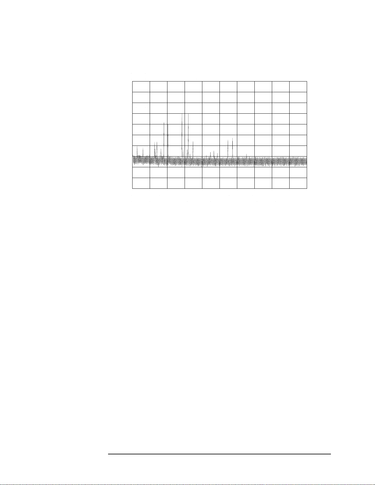
Figure 2-45 Select the band of interest.
Making Measurements
Example 8: External Millimeter Mixers (Unpreselected)
Save the average conversion-loss value
4. Table lists default conversion-loss values that are stored in the
analyzer for each frequency band. These values approximate the
values for the HP 11970 series mixers. Other conversion-loss values
may be entered into the spectrum analyzer in two ways. The first
method lets you to save the average conversion-loss value for the
entire band using
a. Press
CNV LOSS.
AUX CTRL, EXTERNAL MIXER, AMPTD CORRECT, AVERAGE
AVERAGE CNV LOSS. To activate this function:
b. Enter the appropriate average conversion-loss value. On HP
11970 Series harmonic mixers, these values are charted on the
mixer. The U-band mixer used for this example had an average
conversion loss of 23.5 dB, as shown in Figure 2-46.
Chapter 2 99
Page 100
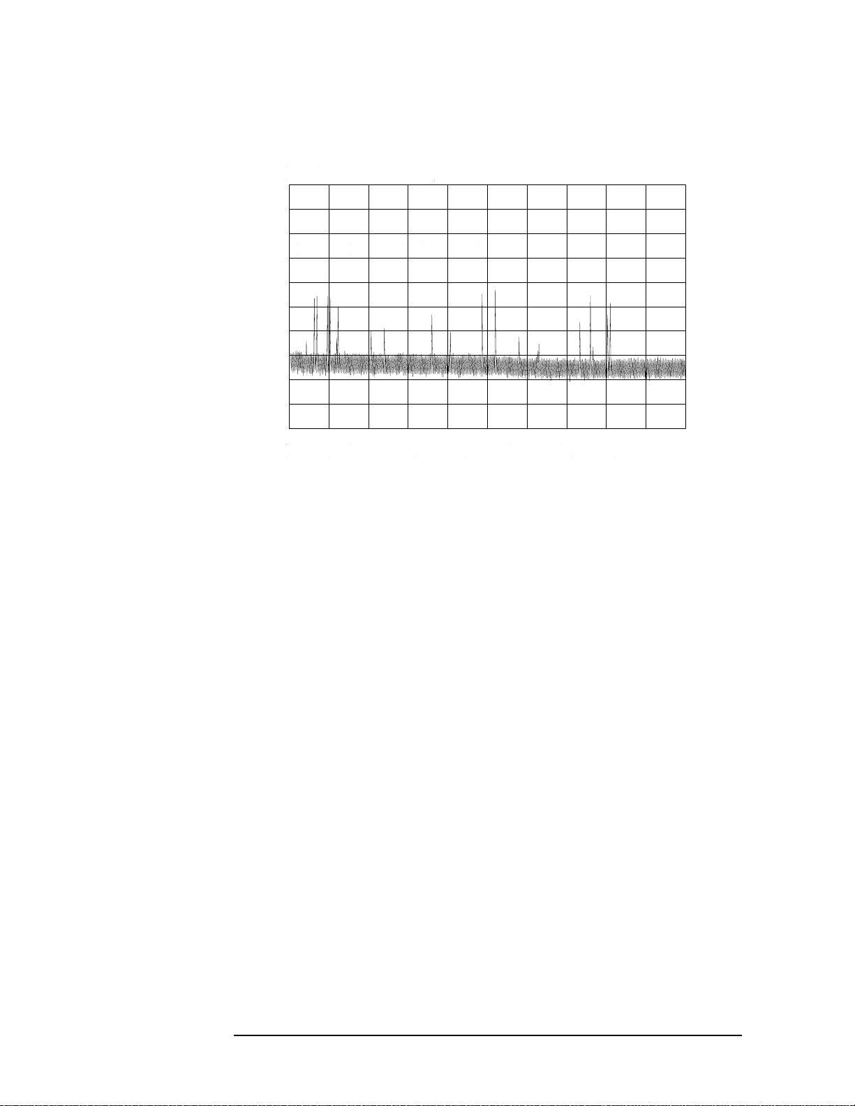
Making Measurements
Example 8: External Millimeter Mixers (Unpreselected)
Figure 2-46 Store and correct for conversion loss.
The second method for storing conversion-loss information lets you
save individual conversion-loss data points at specific intervals
across the harmonic band, using
CNV LOSS VS FREQ.
To view or enter a conversion-loss data point:
a. Press
CNV LOSS VS FREQ.
b. Enter the conversion-loss data at the frequency shown.
c. Use the step up
› key to step through the band, entering the
conversion loss at each step.
Signal Identification (unpreselected mixers only)
5. The IF output of a harmonic mixer contains many mixer products
(frequencies of LO ± source, 2LO ± source, 3LO ± source…nLO ±
source). As a result, within a single harmonic band, a single input
signal can produce many responses, only one of which is valid.
These responses come in pairs, where the members of the valid pair
are spaced 621.4 MHz apart (see Figure 2-47) and the right-most
member for the pair is the correct response (for this analyzer,the left
member of a pair is not valid).
100 Chapter2
 Loading...