Agilent 6100 Familiarization Guide

Download

Agilent 6100 Series Quadrupole LC/MS Systems

Familiarization Guide

Agilent Technologies

Notices

CAUTION

WARNING

No p art o f this manu al may be re produce d in any form or by any means (including electronic storage and retrieval or translation into a foreign language) without prior agreement and written consent from Agilent Technologies, Inc. as governed by United States and international copyright laws.

Manual Part Number

G1960-90080

Edition

Revision A, September 2011

Printed in USA

Agilent Technologies, Inc. 5301 Stevens Creek Blvd. Santa Clara, CA 95051

This guide is valid for the B.03.01 or later revision of the Agilent ChemStation software for the Agilent 6100 Series Quadrupole LC/MS systems, until superseded.

If you have any comments about this guide, please send an e-mail to

feedback_lcms@agilent.com.

Warranty

The material contained in this document is provided “as is,” and is subject to being changed, without notice, in future editions. Further, to the maximum extent permitted by applicable law, Agilent disclaims all warranties, either express or implied, with regard to this manual and any information contained herein, including but not limited to the implied warranties of merchantability and fitness for a particular purpose. Agilent shall not be liable for errors or for incidental or consequential damages in connection with the furnishing, use, or performance of this document or of any information contained herein. Should Agilent and the user have a separate written agreement with warranty terms covering the material in this document that conflict with these terms, the warranty terms in the separate agreement shall control.

Technology Licenses

The hardware and/or software described in this document are furnished under a license and may be used or copied only in accordance with the terms of such license.

Restricted Rights Legend

U.S. Government Restricted Rights. Software and technical data rights granted to the federal government include only those rights customarily provided to end user customers. Agilent provides this customary commercial license in Software and technical data pursuant to FAR 12.211 (Technical Data) and 12.212 (Computer Software) and, for the Department of Defense, DFARS

252.227-7015 (Technical Data - Commercial Items) and DFARS 227.7202-3 (Rights in Commercial Computer Software or Computer Software Documentation).

Safety Notices

A CAUTION notice denotes a hazard. It calls attention to an operating procedure, practice, or the like that, if not correctly performed or adhered to, could result in damage to the product or loss of important data. Do not proceed beyond a CAUTION notice until the indicated conditions are fully understood and met.

A WARNING notice denotes a hazard. It calls attention to an operating procedure, practice, or the like that, if not correctly performed or adhered to, could result in personal injury or death. Do not proceed beyond a WARNING notice until the indicated conditions are fully understood and met.

Agilent 6100 Series Quadrupole LC/MS Systems Familiarization Guide

In this Guide...

This guide presents a series of exercises to help you learn the basic operation of your Agilent 6100 Series LC/MS system.

If you have any comments about this guide, please send an e-mail to feedback_lcms@agilent.com.

1 Prepare for the Analysis

Use these exercises to prepare the LC, to dilute a sulfa demonstration sample, and to check the tune on the MS.

2 Set Up and Run a Scan Method

Learn how to set up a scan method and acquire data for the sulfa demonstration mix.

3 Qualitative Data Analysis

Learn how to examine chromatograms and spectra to identify sample components. In these exercises, you review data from the sulfa sample you analyzed in Chapter 2, or from a data file that you received with your ChemStation software.

4 Set Up and Run a SIM Method

Learn how to set up a selected ion monitoring (SIM) method and acquire data for the sulfa demonstration mix.

5Set Up and Run a Sequence

Use these exercises to set up an automated sequence for SIM analyses of the sulfa mix at various concentrations, and to acquire data with that sequence.

6 Quantitative Data Analysis

Learn how to analyze data when you need to quantify sample components. These exercises use caffeine data files that you received with your ChemStation software.

Agilent 6100 Series Quadrupole LC/MS Systems Familiarization Guide 3

4 Agilent 6100 Series Quadrupole LC/MS Systems Familiarization Guide

Contents

1 Prepare for the Analysis 7

Exercise 1. Prepare the LC to run the sample 8

Task 1. Start up ChemStation 8 Tas k 2 . P ur ge t he pu mp 9 Task 3. Prepare the column for the analyses 10

Exercise 2. Prepare the samples for the analyses 12

Exercise 3. Check the current MS tune values and adjust if

necessary 14

2 Set Up and Run a Scan Method 15

Exercise 1. Set up a full-scan acquisition method 16

Task 1. Enter LC acquisition parameters 16 Task 2. Enter MS acquisition parameters 19

Exercise 2. Acquire data with the full-scan method 23

Task 1. Enter sample information 24 Task 2. Acquire the data 25

3 Qualitative Data Analysis 27

Exercise 1. Display and manipulate chromatograms 28

Exercise 2. Examine mass spectra 31

Exercise 3. Integrate the chromatogram 36

Exercise 4. Print a report 40

4 Set Up and Run a SIM Method 43

Exercise 1. Set up a SIM acquisition method 44

Agilent 6100 Series Quadrupole LC/MS Systems Familiarization Guide 5

Contents

Task 1. Load the scan method you created previously 44 Task 2. Enter MS acquisition parameters 45

Exercise 2. Acquire data with the SIM method 48

Task 1. Enter sample information 49 Task 2. Acquire the data 50

5Set Up and Run a Sequence51

Exercise 1. Set up a sequence 52

Task 1. Prepare to create a new sequence 52 Task 2. Edit sequence parameters 53 Task 3. Set up the sequence table 55 Task 4. Set up the sequence output 58

Exercise 2. Run the sequence 60

6 Quantitative Data Analysis 61

Exercise 1. Create a method for quantification 62

Task 1. Create a new method 62 Task 2. Set up the signal for quantification 63 Task 3. Integrate the low-level standard 65 Task 4. Set general calibration parameters 67 Task 5. Set up the calibration curve 68 Task 6. Explore options to refine the calibration 72

Exercise 2. Process a sample and print a report 73

6 Agilent 6100 Series Quadrupole LC/MS Systems Familiarization Guide

Agilent 6100 Series Quadrupole LC/MS System Familiarization Guide

1 Prepare for the Analysis

Exercise 1. Prepare the LC to run the sample 8

Task 1. Start up ChemStation 8 Task 2. Purge the pump 9

Task 3. Prepare the column for the analyses 10 Exercise 2. Prepare the samples for the analyses 12 Exercise 3. Check the current MS tune values and adjust if necessary 14

This chapter presents exercises to help you learn how to:

• Prepare the LC and column for an analysis

• Prepare the samples that you analyze in these exercises

• Check the tune settings of the MS and adjust if necessary.

Before you start

• Order the sample: Agilent Electrospray LC Demo Sample,

p/n 59987-20033.

• Order the column: Agilent ZORBAX SB-C18, 2.1 mm x 30 mm,

3.5 µm, p/n 873700-902.

• You may use another similar column, but you may need to adjust the HPLC conditions to obtain good separation.

• Make sure that the electrospray source is installed.

• Read the Agilent 6100 Series Quadrupole LC/MS Systems

Quick Start Guide and Chapter 2 of the Agilent 6100 Series Quadrupole LC/MS Systems Concepts Guide.

Agilent Technologies

1 Prepare for the Analysis

Exercise 1. Prepare the LC to run the sample

For the following tasks, try the steps in the first column. If you need more help, follow the detailed instructions in the middle column.

Task 1. Start up ChemStation

Steps Detailed Instructions Comments

1 Open the ChemStation window. • Click the ChemStation icon on the

desktop.

Alternate method:

• From the Start menu, select:

All Programs > Agilent ChemStation > Instrument 1 online.

8 Agilent 6100 Series Quadrupole LC/MS Systems Familiarization Guide

Prepare for the Analysis 1

Task 2. Purge the pump

Use these instructions with the binary and quaternary pumps. See the ChemStation online Help for instructions for the capillary and nanoflow pumps.

Steps Detailed Instructions Comments

1 Display the Method and Run Control

view.

2 Place the pump in standby mode. a Click More Pump > Control HPLC

3 Prepare solvents used in these

familiarization exercises.

• A – 5 mM ammonium formate in

water

• B – 5 mM ammonium formate in

methanol

4 Replace the solvent bottles with the

ones you just prepared.

5 Open the purge valve. a Turn the black purge valve on the

6 Enter a flow of 5 mL/min and

50% B, using water in channel A and methanol in channel B.

• In the view selection area in the lower left, click Method and Run

Control.

Pump on the Instrument menu to

open the Pump Control dialog box.

b Select Standby and click OK.

a Into a 1-liter reservoir of

HPLC-grade water, add 1 mL of 5 M ammonium formate.

b Into a 1-liter reservoir of

HPLC-grade methanol, add 1 mL of 5 M ammonium formate.

• Replace the bottles for channels A and B.

front of the pump counter-clockwise two turns.

b Place the tubing that exits the pump

into a 250-mL or larger beaker.

a Click the pump icon. b Select Set up Pump. c Enter the parameters in step 6 and

click OK.

Alternate method:

• Select Standby from the Pump context menu.

• The part number for ammonium formate is G1946-85021.

• Each ampoule contains 2.2 mL of ammonium formate solution.

• Be sure to use HPLC-grade solvents.

7 Turn the pump on and monitor the

tubing for bubbles.

a To turn the pump on, click the

little button to the lower right of the solvent delivery (pump) icon.

b Monitor for bubbles.

• Purge for about 3 minutes to pass

3X the volume for the binary pump.

• If you wish, you may purge each channel individually first, to ensure that neither is air-locked.

Agilent 6100 Series Quadrupole LC/MS Systems Familiarization Guide 9

1 Prepare for the Analysis

Task 3. Prepare the column for the analyses

Steps Detailed Instructions Comments

8 After the bubbles are gone and the

purge is complete, enter a flow of 1 mL/min and 100% B.

9 Purge a short while longer, and then

close the purge valve.

a Right-click the pump icon. b Select Set up pump. c Enter the new parameters in step 8,

and click OK.

a Continue to purge for a short while. b Close the black valve.

For more information on purging the pump, see the reference manual that you received with your pump.

Task 3. Prepare the column for the analyses

In the exercises in the next chapters, you analyze a mixture of four sulfonamide compounds. To perform the analyses in the following chapters, you must first condition and equilibrate your column.

Steps Detailed Instructions Comments

1 Disconnect the column from the

detector and MS.

a Turn the pump off by clicking

the little button to the lower right of the solvent delivery (pump) icon.

b Disconnect the column from the

detector and MS.

c Place the open end of the tubing

that exits the column into the beaker.

• To prevent detector contamination, allow the column effluent to go directly to the waste beaker.

2 Flush the column with 100%

methanol at 1 mL/min (5 to 10 min).

• ZORBAX SB-C18, 2.1 mm

3.5 µm, p/n 873700-902

× 30 mm,

a Tur n t h e pum p o n. b Flow methanol through the column

under the conditions used in Task 2,

step 8.

• The data sheet shipped with the column cartridge recommends that you flush with 20 to 30 columnvolumes of 100% methanol (approximately 5 to 7.5 mL).

10 Agilent 6100 Series Quadrupole LC/MS Systems Familiarization Guide

Prepare for the Analysis 1

Task 3. Prepare the column for the analyses

Steps Detailed Instructions Comments

3 Condition the column as follows,

using the solvents made up in Task 2,

step 6:

• Flow rate – 0.4 mL/min

• 100% B for 1/2 hour

• 50% B for 1/2 hour

4 Equilibrate the column at the analysis

conditions:

• 12% B for 1/2 hour at 40 °C

5 While the column equilibrates, set

parameters for the MS spray chamber so it can heat and equilibrate as well.

• Drying gas flow: 8 L/min

• Nebulizer pressure: 35 psig

• Drying gas temperature: 300

• Capillary voltage: 3000 V

For 6150 with Agilent Jet Stream technology:

• Sheath Gas Flow: 12 L/min

• Sheath Gas Temp: 360°C

• Nozzle Voltage: 0 V

a Click Set up Instrument Method on

the Instrument menu to open the Setup Method dialog box.

b Click the Pump tab. c Enter the flow rate in step 3. d For Solvent B, type 100 and click

Apply. e Wait 30 minutes. f For Solvent B, type 50 and click

Apply. g Wait 30 minutes.

a For Solvent B, type 12 and click

OK. b Click the TCC tab on the Setup

Method dialog box.

c For Temperature, type 40 and click

OK.

a Right-click the MSD

icon on the system

diagram and select

Spray Chamber. b Enter the parameters described in

step 5.

c Click OK. d Wait 10 minutes before you tune the

MS.

• At a flow rate of 0.4 mL/min, the checkout column should produce about 70 to 80 bar pressure (measured without any fittings at the column exit).

• If, after you perform these steps, the pump pressure through the column is too high, order a replacement SB-C18 column (p/n 873700-902).

• If your column is not new, you can reduce the length of time that you condition the column.

• While you condition and equilibrate the column, you may complete

step 5 in this exercise and then

work on the rest of the exercises in this chapter. Be sure to complete

step 6 before you go on to the next

chapter.

6 Reconnect the column to the DAD

and MS.

• You can complete “Exercise 3.

Check the current MS tune values and adjust if necessary” either with

or without the column connected to the DAD and MS, but you do need to reconnect prior to the exercises in

Chapter 2, “Set Up and Run a Scan

Method.”

Agilent 6100 Series Quadrupole LC/MS Systems Familiarization Guide 11

1 Prepare for the Analysis

Exercise 2. Prepare the samples for the analyses

In the exercises in the next chapters, you analyze a mixture of four sulfonamide compounds. The Electrospray LC Demo Sample (p/n 59987-20033), contains five ampoules with 100 ng/µL each of these compounds:

• sulfamethizole (M+H)

• sulfamethazine (M+H)

• sulfachloropyridazine (M+H)

• sulfadimethoxine (M+H)

= 271

= 279

= 311.

= 285

Sulfamethizole Sulfamethazine Sulfachloropyridazine Sulfadimethoxine

To perform the analyses in the following chapters, you must first prepare the sample at various dilutions. The final concentrations will be 1, 5 and 10 ng/µL. You will also prepare a solvent blank.

12 Agilent 6100 Series Quadrupole LC/MS Systems Familiarization Guide

Prepare for the Analysis 1

Exercise 2. Prepare the samples for the analyses

Steps Detailed Instructions Comments

1 Prepare a 1:10 dilution of the original

sample in a 1-mL autosampler vial.

• Final concentration is 10 ng/µL

• You will use this sample for the

scan analysis in Chapter 2, and for the SIM analyses in Chapter 4 and

Chapter 5.

2 Prepare a 1:20 dilution of the original

sample in a 1-mL autosampler vial.

• Final concentration is 5 ng/µL

• You will use this sample for the SIM

analysis in Chapter 5.

3 Prepare a 1:100 dilution of the original

sample in a 1-mL autosampler vial.

• Final concentration is 1 ng/µL

• You will use this sample for the SIM

analysis in Chapter 5.

4 Prepare a solvent blank in a 1-mL

autosampler vial.

• You will use this sample for the SIM

analysis in Chapter 5.

a Transfer 100 µL of the sulfa mixture

into the autosampler vial.

b Add 900 µL of 90:10 water:methanol

that contains 5 mM ammonium formate (NH

c Cap the vial.

a Transfer 50 µL of the sulfa mixture

into the autosampler vial.

b Add 950 µL of 90:10 water:methanol

that contains 5 mM ammonium formate.

c Cap the vial.

a Transfer 10 µL of the sulfa mixture

into the autosampler vial.

b Add 990 µL of 90:10 water:methanol

that contains 5 mM ammonium formate.

c Cap the vial.

a Into the autosampler vial, transfer

990 µL of 90:10 water:methanol that contains 5 mM ammonium formate.

b Cap the vial.

HCO2).

• The original sulfa mixture is dissolved in a solvent mixture of 70% water and 30% acetonitrile.

Agilent 6100 Series Quadrupole LC/MS Systems Familiarization Guide 13

1 Prepare for the Analysis

Exercise 3. Check the current MS tune values and adjust if necessary

The MS is very stable and does not need to be tuned very often. You can usually tune just once a month, or once a week at most. You can use the Check Tune program described in this exercise to confirm that the MS is in adjustment.

Steps Detailed Instructions Comments

1 Switch to the MSD Tune view. • In the view selection area in the

lower left, click MSD Tune.

2 Select the tune file. a In the Select Tune File dialog box,

select ATU NE S.TU N.

b Keep the default of Positive Polarity

(Standard). c Click OK. d In the status bar near the top of the

MSD Tune view, verify that you see

the following:

• Mode is API-ES

• Source is ESI (electrospray)

3 Run a Check Tune. • From the Tune menu, select Check

Tune.

Note that Check Tune requires

values for comparison that are

determined from a previous

Autotune. Autotune is normally run

during installation.

4 If Check Tune report suggests that

you adjust peak widths or mass axis, then do that.

5 If the Check Tune report shows poor

sensitivity, which indicates that your MS settings are significantly out of adjustment, then run a full Autotune.

a From the Tune menu, select Adjust

Mass Peak Width. b From the Tune menu, select

Calibrate Mass Axis.

• From the Tune menu, select

Autotune > Positive Polarity.

• Make sure that you use an

appropriate calibrant with an appropriate source.

• Check Tune is normally all that you need to do to confirm that the MS settings are correct.

• If Check Tune indicates a problem with your MS settings, then proceed to step 4 and/or step 5.

• The exercises in this manual use only the positive ion mode and standard scan speeds, so it is not necessary to tune for negative polarity or fast scan.

14 Agilent 6100 Series Quadrupole LC/MS Systems Familiarization Guide

Agilent 6100 Series Quadrupole LC/MS System Familiarization Guide

2 Set Up and Run a Scan Method

Exercise 1. Set up a full-scan acquisition method 16

Task 1. Enter LC acquisition parameters 16 Task 2. Enter MS acquisition parameters 19

Exercise 2. Acquire data with the full-scan method 23

Task 1. Enter sample information 24 Task 2. Acquire the data 25

These exercises show you how to set up a scan data acquisition method for the demonstration sample (sulfa mix) and to acquire data with that method.

The LC parameters that you enter in these exercises are appropriate for the standard Agilent 1100/1200/1260/1290 Series liquid chromatography (LC) systems. You must enter LC parameters that are appropriate for your LC model.

To view the results of these exercises, see Chapter 3, “Qualitative Data Analysis.”

Before you start

• Review the Agilent 6100 Series Quadrupole LC/MS Systems Quick Start Guide and Chapter 3 of the Agilent 6100 Series Quadrupole LC/MS Systems Concepts Guide.

• Prepare the LC, column and sample as described in

Chapter 1, “Prepare for the Analysis.”

For the tasks on the following pages, try the steps on the left without the detailed instructions. If you need more help, follow the detailed instructions on the right.

Agilent Technologies

2 Set Up and Run a Scan Method

Exercise 1. Set up a full-scan acquisition method

This exercise changes the default method and saves it as a new method. This exercise consists of the following tasks:

• “Task 1. Enter LC acquisition parameters” on page 16

• “Task 2. Enter MS acquisition parameters” on page 19

Task 1. Enter LC acquisition parameters

Steps Detailed Instructions Comments

1 Display the Method and Run Control

view.

2 Open the method DEF_LC.M. a Select File > Load > Method.

3 Save the method under a new name,

SULFAMSSCAN1.M.

4 Enter a volume of

injection.

1 µL for the

• In the view selection area in the

lower left of the ChemStation window, click Method and Run

Control.

b If necessary, navigate to

C:\CHEM32\1\METHODS.

c Select DEF_LC.M and click OK.

a Select File > Save As > Method. b In the dialog box, for Name, type

SULFA MS SCAN 1.M.

c Click OK. d In the box for Comment for method

history, type a comment.

e Click OK.

a Click Set up Instrument Method on

the Instrument menu to open the Setup Method dialog box.

b Click the ALS tab. c Click Standard injection. d In the Injection volume box, type 1

for a 1-µL injection.

• You save the method now with a new name to avoid inadvertently overwriting the default method later.

16 Agilent 6100 Series Quadrupole LC/MS Systems Familiarization Guide

Set Up and Run a Scan Method 2

Task 1. Enter LC acquisition parameters

Steps Detailed Instructions Comments

5 Enter pump parameters. a Click the Pump tab on the Setup

Method dialog box.

b Set the parameters as follows:

Flow=0.400mL/min StopTime=7.00 min PostTime=3.00min

Solvent A=Water 88% Solvent B=Methanol 12%

6 Set up the gradient timetable as it

appears in the figure below.

7 Enter a column compartment

temperature of 40

8 Enter parameters for the diode-array

detector (DAD).

a Open the Timetable area in the

lower part of the tab, click Insert, and type the first line.

b Click Append and type the second

line.

c Repeat step b for lines 3 and 4.

a Click the TCC tab on the Setup

Method dialog box.

b Click the option button for oC. c Ty p e 40.0 for

a Click the DAD tab on the Setup

Method dialog box.

b Enter the parameters shown below:

• Use Signal A: Wavelength 272nm,

Bandwidth16 nm

• Reference Wavelength: 360 nm,

Reference Bandwidth 100 nm

• Spectrum Store: All in peak

• Peakwidth: > 0.1 min

c Click OK to close the Setup Method

dialog box with the new setpoints.

Set the timetable parameters as follows:

Line 1 Time 1:00, %B=12, Flow=0.4 Line 2 Time 3:00, %B=100, Flow=0.4 Line 3 Time 6:00, %B=100, Flow=0.4 Line 4 Time 7:00, %B=12, Flow=0.4

• The DAD is used in this example, but the variable wavelength detector (VWD) may be used analogously.

Agilent 6100 Series Quadrupole LC/MS Systems Familiarization Guide 17

2 Set Up and Run a Scan Method

Task 1. Enter LC acquisition parameters

Steps Detailed Instructions Comments

9 Select Data Acquisition only in the

Run Time Checklist.

10 Save the new parameters to the

method file, SULFA MS SCAN 1.M.

a Click Run Time Checklist on the

RunControl menu.

b Mark the Data Acquisition check

box.

c Click OK.

a Select File > Save > Method. b In the box for Comment for method

history, type a comment.

c Click OK.

• While it is common to include Data

Analysis in the Run Time Checklist, for these exercises, you will view the results in Chapter 3, “Qualitative Data Analysis.”

18 Agilent 6100 Series Quadrupole LC/MS Systems Familiarization Guide

Set Up and Run a Scan Method 2

Set to 100 for 6120 Set to 125 for 6130 or 6150

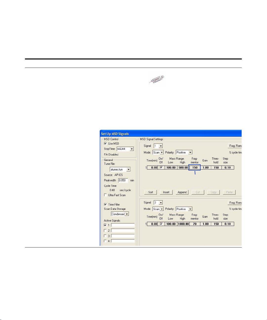
Task 2. Enter MS acquisition parameters

Steps Detailed Instructions Comments

1 Enter parameters for the quadrupole

mass spectrometer (MS):

• Signal 1, scan mode, positive

polarity

• Scan range: 100 to 500

• Fragmentor:

100 V for the Agilent 6120; 125 V for the 6130 or 6150

• Gain: 1.00

• Threshold: 150

• Stepsize: 0.10

• Peakwidth: 0.05 min

• Scan data storage: Condensed

• Active signals: 1 only

a Right-click the MSD

icon on the system diagram and select Set

up MSD Signals.

b Enter the parameters described in

step 1 and shown in the figure

below. Take care to enter the appropriate Fragmentor voltage for your MS model.

c Click OK.

• To save disk space you usually acquire line spectra (Scan Data Storage = Condensed). However,

when you acquire spectra from intact proteins or protein digests/peptides, you must acquire and deconvolute profile spectra. (Scan Data Storage = Full).

Agilent 6100 Series Quadrupole LC/MS Systems Familiarization Guide 19

2 Set Up and Run a Scan Method

Task 2. Enter MS acquisition parameters

Steps Detailed Instructions Comments

2 Enter parameters for the spray

chamber of the ion source:

• Drying gas flow: 9 L/min

• Nebulizer pressure: 40 psig

• Drying gas temperature: 300

• Capillary voltage: 3000 V

For 6150 with Agilent Jet Stream technology:

• Nebulizer pressure: 30 psi

• Drying gas flow: 7 L/min

• Drying gas temperature: 350°C

• Sheath gas flow: 12 L/min

• Sheath gas temperature: 360 C°

• Capillary voltage: 4000 V

• Nozzle voltage: 0 V

• Fragmentor: 200 V

• Multiplier gain: 3

a Right-click the MSD

icon on the system diagram and select

Spray Chamber.

b Enter the parameters described in

step 2 and shown in the figure

below.

c Click OK.

For all models except 6150 with Agilent Jet Stream technology

For 6150 with Agilent Jet Stream technology

20 Agilent 6100 Series Quadrupole LC/MS Systems Familiarization Guide

Set Up and Run a Scan Method 2

Task 2. Enter MS acquisition parameters

Steps Detailed Instructions Comments

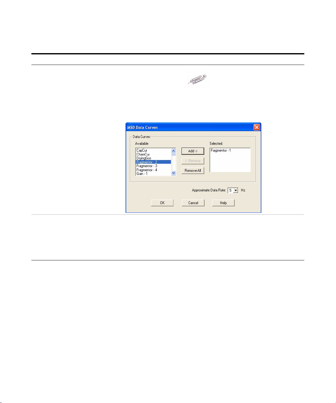
3 Set up to store the fragmentor voltage

throughout the run.

4 Save the method. a Select Method > Save Method to

a Right-click the MSD

icon on the system diagram and select

Data Curves. b Select Fragmentor - 1. c Click the Add button. d Click OK.

overwrite the method

SULFA MS SCAN 1.M. b In the box for Comment for method

history, type a comment. c Click OK.

Agilent 6100 Series Quadrupole LC/MS Systems Familiarization Guide 21

2 Set Up and Run a Scan Method

Task 2. Enter MS acquisition parameters

Steps Detailed Instructions Comments

5 Print the method. a Select Method > Print Method.

b Mark the check boxes as shown in

the figure below.

c Click the Print button.

22 Agilent 6100 Series Quadrupole LC/MS Systems Familiarization Guide

Set Up and Run a Scan Method 2

Exercise 2. Acquire data with the full-scan method

Now you are ready to acquire data for the sulfa mix with the method you just created. This exercise consists of the following tasks:

• “Task 1. Enter sample information” on page 24

• “Task 2. Acquire the data” on page 25

Agilent 6100 Series Quadrupole LC/MS Systems Familiarization Guide 23

2 Set Up and Run a Scan Method

Task 1. Enter sample information

Steps Detailed Instructions Comments

1 Display the Single Sample toolbar. • In the top toolbar, click

the single sample icon.

1 Display the Sample Information dialog

box.

2 Enter the sample information:

• Operator name

• Subdirectory: Sulfas

• Prefix: Sulfa_scan

• Location: Vial 1

• Sample Name: Sulfas 10 ng/µ

• Comment: Scan familiarization

exercise

a Click Sample Info on the

RunControl menu.

a Enter the parameters described in

step 2 and shown in the figure

below.

b Click OK.

• If you select Prefix/Counter, the

file names increment automatically from one run to the next.

24 Agilent 6100 Series Quadrupole LC/MS Systems Familiarization Guide

Set Up and Run a Scan Method 2

Task 2. Acquire the data

Steps Detailed Instructions Comments

1 Place the vial of sulfa sample you

prepared at 10 ng/µL into position 1 in the autosampler.

2 Inject the sulfa mix sample. • Click the Single Sample button to

start the run.

3 Monitor the total ion chromatogram

and the UV chromatogram during data acquisition.

a From the Online Plot window, click

the Change button. b In the list of Available Signals,

select DAD A: Signal=272,16

Reference=360,100 and click Add. c In the list of available signals, select

MSD: Signal 1 and click Add. d Monitor the MS signal to ensure a

stable baseline.

• You prepared this sample in

“Exercise 2. Prepare the samples for the analyses” on page 12.

This button is present only when you have selected Single Sample mode from the top toolbar.

• If the baseline fluctuation for the MS signal is greater than 10%, the nebulizer and source chamber may require maintenance. See the

Agilent 6100 Series Single Quad LC/MS System Maintenance Guide.

Agilent 6100 Series Quadrupole LC/MS Systems Familiarization Guide 25

2 Set Up and Run a Scan Method

Task 2. Acquire the data

Steps Detailed Instructions Comments

4 Save the signals for the Online Plot

window.

5 When the analysis is done, view the

results.

a In the Edit Signal Plot dialog box,

click the Apply to Method button.

b Save the method.

• To view the results, go to the next

exercise.

• The C18 column may require one or two injections of the sample to be fully conditioned. During these initial injections, everything may be eluted from the column in the void volume. Repeat the process and separation will occur.

26 Agilent 6100 Series Quadrupole LC/MS Systems Familiarization Guide

Agilent 6100 Series Quadrupole LC/MS System Familiarization Guide

3 Qualitative Data Analysis

Exercise 1. Display and manipulate chromatograms 28 Exercise 2. Examine mass spectra 31 Exercise 3. Integrate the chromatogram 36 Exercise 4. Print a report 40

This chapter shows you how to analyze data when you need to identify or confirm sample components.

These exercises use the data file you generated in Chapter 2. Alternatively, you can use the sulfa demo data file that you received with the ChemStation software.

Before you start

• Read the Agilent 6100 Series Quadrupole LC/MS Systems Quick Start Guide.

• Read the chapter on Data Analysis in the Agilent 6100 Series Quadrupole LC/MS Systems Concepts Guide.

• Set up and run the acquisition method in Chapter 2, “Set Up and Run a Scan Method” or that you have the mssulfas.d data file in the MSDEMO data folder on your system.

For the tasks on the following pages, perform the exercises in the order they appear. Try the steps on the left without the detailed instructions. If you need more help, follow the detailed instructions on the right.

Agilent Technologies

3 Qualitative Data Analysis

Exercise 1. Display and manipulate chromatograms

In this exercise, you load chromatograms and change the chromatographic display.

Steps Detailed Instructions Comments

1 Display Data Analysis view. • In the view selection area of the

ChemStation window, click Data Analysis.

2 Load the method

SULFAMSSCAN1.M.

3 Display the Signal Toolset. • Click the Signal icon,

a Select File > Load > Method. b Navigate to the folder

C:\CHEM32\1\METHODS.

c Select the method file and click OK.

which is near the middle of the window.

• If you just completed the previous exercise, that method is already loaded.

28 Agilent 6100 Series Quadrupole LC/MS Systems Familiarization Guide

Qualitative Data Analysis 3

Exercise 1. Display and manipulate chromatograms

Steps Detailed Instructions Comments

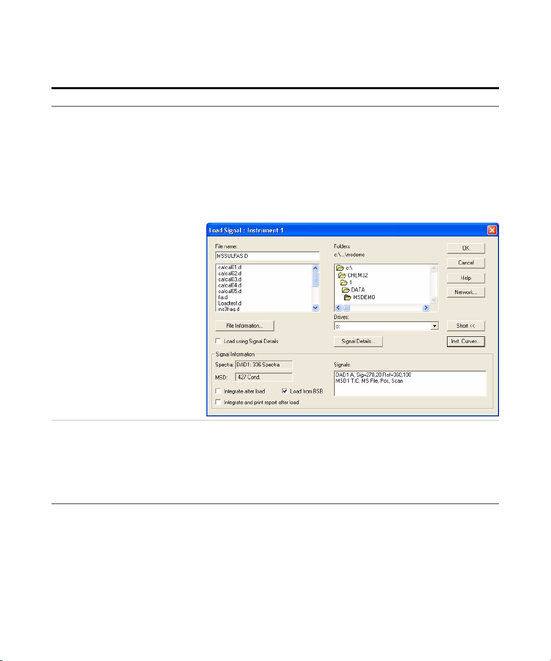
4 Do one of the following:

• Open the data file,

SULFA_SCAN00001.D, which you

acquired in Chapter 2.

• Open the data file mssulfas.d,

located in the MSDEMO folder.

a Select File > Load Signal. b Navigate to the appropriate folder,

either:

• C:\CHEM32\1\DATA\SULFAS,

• C:\CHEM32\1\DATA\MSDEMO.

c Select the data file. d Set other parameters as shown

below and click OK.

• For other ways to load signals, see

the Data Analysis chapter in the Concepts Guide.

• If you wish to complete Chapter 4, “Set Up and Run a SIM Method”, then you need to process the data file you generated in Chapter 2. You need the report from that data file to set up your SIM groups.

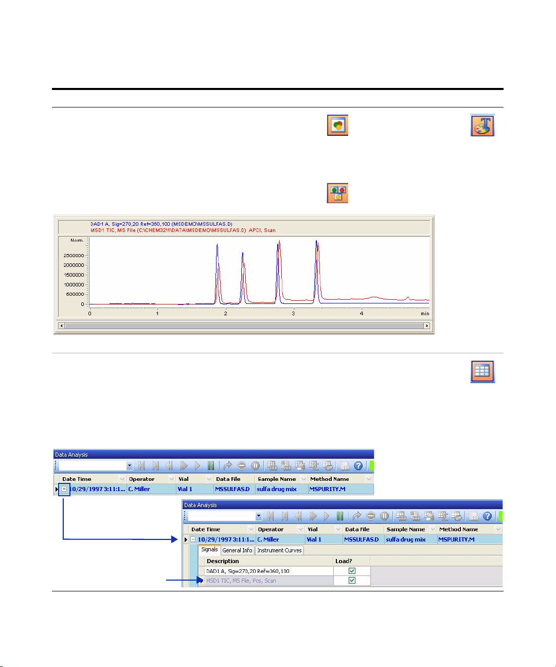
5 Verify that you see the DAD and MS

chromatograms.

a Check that you see a display that is

similar to the one shown below.

b Verify that you see the DAD signal

in the top chromatogram.

c Confirm that you see the MSD

signal in the bottom chromatogram.

Agilent 6100 Series Quadrupole LC/MS Systems Familiarization Guide 29

3 Qualitative Data Analysis

Exercise 1. Display and manipulate chromatograms

Steps Detailed Instructions Comments

6 Change the chromatogram view so

that the MS and UV chromatograms are overlaid in the display.

7 Remove the DAD signal from the

display.

a In the Signal Toolset near

the middle of the window, click the icon to display overlaid signals.

b Check that you see the overlaid

chromatograms, as shown below.

c Click the icon to display

separate signals.

a In the Navigation Table, click the +

to display more information.

b Under the Signals tab, double-click

the signal labeled MSD1 TIC.

c When you see the message about

the method, click OK.

d Verify that the DAD window is gone

and only the TIC is displayed.

• The icon in step a is also available in the Graphics Toolset, but in that toolset it toggles overlaid/separate. You click the icon shown above to turn on the display of the Graphics Toolset.

• If you do not see the Navigation Table shown below, in the top toolbar, click the icon shown above.

• For other ways to remove signals, see the chapter on Data Analysis in the Concepts Guide.

30 Agilent 6100 Series Quadrupole LC/MS Systems Familiarization Guide

Qualitative Data Analysis 3

Exercise 2. Examine mass spectra

In this exercise, you learn to display mass spectra. You choose background (reference) spectra that you can later subtract from the spectra of the peaks of interest. You learn how to display a single spectrum and an averaged spectrum for a peak.

Steps Detailed Instructions Comments

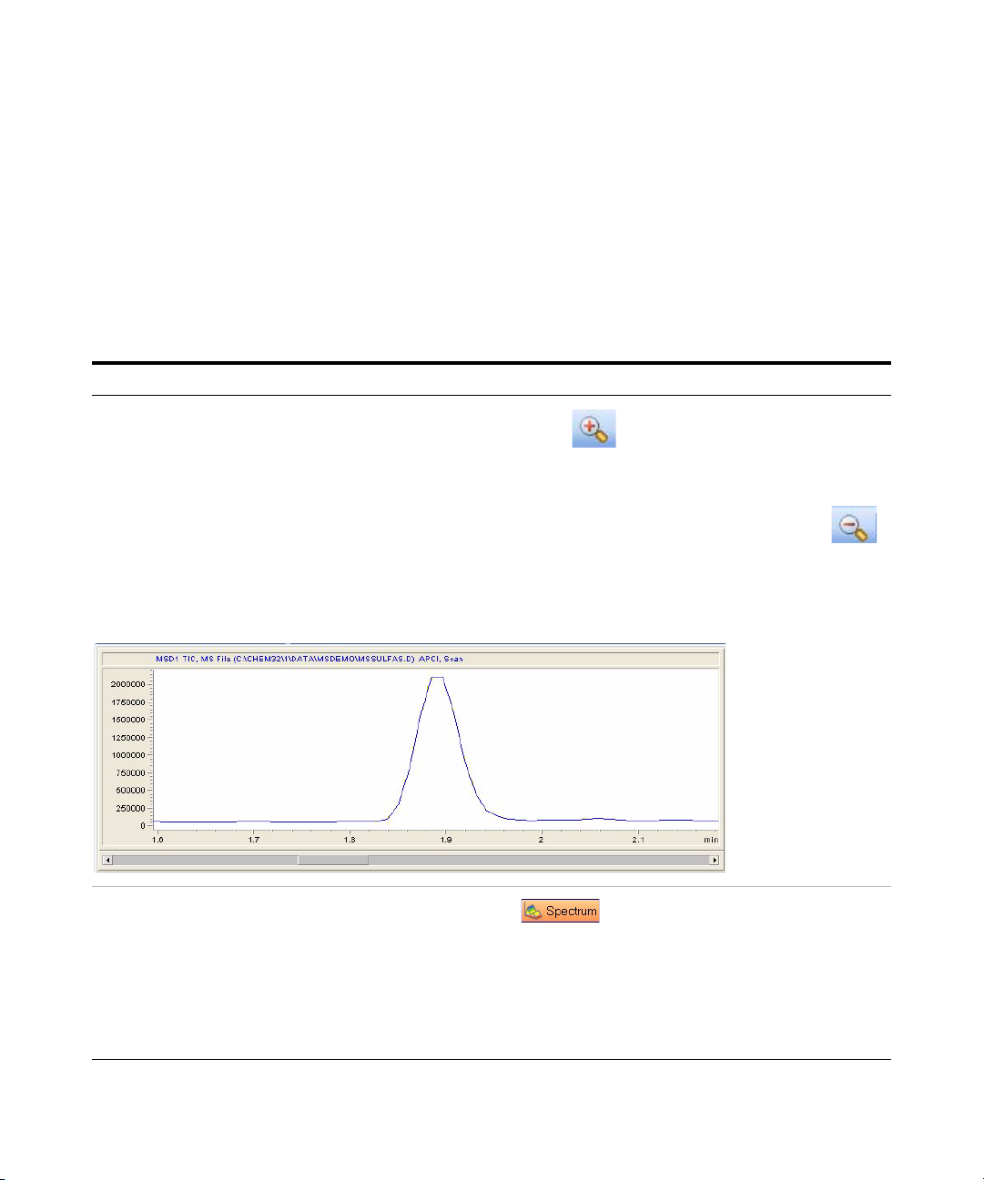
1 Zoom in on the first peak in the

chromatogram.

2 Display the Spectrum Toolset. a Click the Spectrum

a Click the icon to zoom in. b Use the mouse pointer to

draw a rectangle around the peak. Take care to include the chromatographic baseline.

c Check that your peak looks similar

to the one below.

d Note the width of the peak at half

height. You will need this information to set up the SIM analysis in Chapter 4.

icon, which is near the middle of the window.

b If there is not room under your

chromatogram window to display spectra, use your mouse pointer to reduce the height of the chromatogram window.

• If you want to try again, you can zoom back out. Do one of the following:

• Double-click the chromatogram

window.

• Click the icon to zoom

out.

Agilent 6100 Series Quadrupole LC/MS Systems Familiarization Guide 31

3 Qualitative Data Analysis

Exercise 2. Examine mass spectra

Steps Detailed Instructions Comments

3 Get the first reference spectrum, to

the left of the peak.

4 Get a second reference spectrum, to

the right of the peak.

5 View your reference spectra. a If you cannot see the spectra, adjust

a To s e le ct th e f ir st

reference spectrum, click the icon that is highlighted here.

b In the chromatogram window, do

one of the following at the chromatographic baseline just before the peak:

• Click to select a single spectrum.

• Click and drag to select an

average spectrum.

a To select the second

reference spectrum, click the icon that is highlighted here.

b In the chromatogram window, do

one of the following at the chromatographic baseline just after the peak:

• Click to select a single spectrum.

• Click and drag to select an

average spectrum.

the size and location of the window labeled Reference Mass

Spectrum(a).

b Note the two background spectra

— one before the peak and one after.

32 Agilent 6100 Series Quadrupole LC/MS Systems Familiarization Guide

Qualitative Data Analysis 3

Exercise 2. Examine mass spectra

Steps Detailed Instructions Comments

6 Set the spectral options to do manual

background subtraction.

a Click the icon to display the

Spectral Options dialog box.

b Click the MS Reference tab. c Under Reference Spectrum, click

Manual.

d Mark the check boxes for Ref1 and

Ref2. Note that the time ranges of

the reference spectra that you just selected are specified there.

e Click OK.

• The spectral options apply to all

subsequent spectra until you change the options.

• If the chromatographic baseline changes over the course of the run, select new reference spectra that are close in time to each peak of interest.

• Near the middle of the Data Analysis window, you can view and change the setting for background subtraction.

Agilent 6100 Series Quadrupole LC/MS Systems Familiarization Guide 33

3 Qualitative Data Analysis

Exercise 2. Examine mass spectra

Steps Detailed Instructions Comments

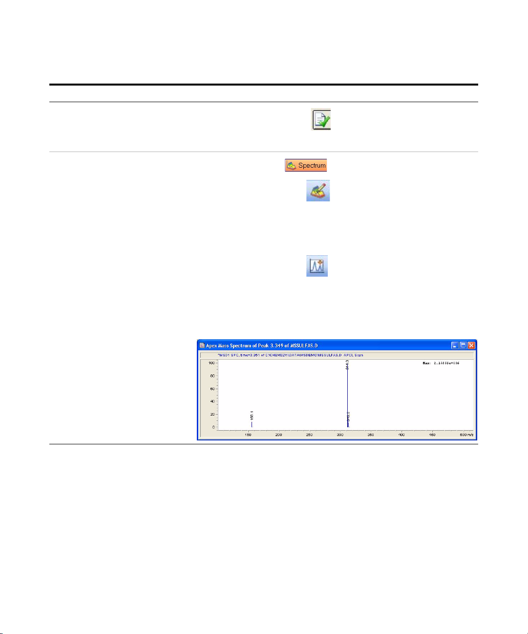
7 Get a single background-subtracted

spectrum for the first LC peak.

a Click the icon to get a mass

spectrum at any time point.

b In the chromatogram

window, click somewhere on the peak to get the spectrum.

c If necessary for easier viewing,

adjust the size and location of the window labeled MS Spectrum.

d Verify that the spectrum is similar to

the one shown below.

• Under the conditions used to acquire the demo data file (mssulfas.d), the compounds elute in the following order:

Sulfamethizole, m/z = 271 Sulfachloropyridazine, m/z = 285 Sulfamethazine, m/z = 279 Sulfadimethoxine, m/z = 311

• Depending on the organic mobile phase and the modifiers, the elution order for the 279 and 285 may change.

34 Agilent 6100 Series Quadrupole LC/MS Systems Familiarization Guide

Qualitative Data Analysis 3

Exercise 2. Examine mass spectra

Steps Detailed Instructions Comments

8 Get a average background-subtracted

spectrum for the first LC peak.

9 Be sure to see step 6 in “Exercise 3.

Integrate the chromatogram” for an

easier, faster way to display spectra.

a Click the icon to get an

averaged mass spectrum.

b In the chromatogram

window, click and drag the mouse across the peak, as shown below.

c View the average spectrum in the

window labeled MS Spectrum.

• When a chromatographic peak consists of a single compound, an average spectrum is usually more accurate.

Agilent 6100 Series Quadrupole LC/MS Systems Familiarization Guide 35

3 Qualitative Data Analysis

Exercise 3. Integrate the chromatogram

In this exercise, you learn to set integration events and integrate the chromatogram. Even if you do not care about quantitation, integration helps locate peaks for other purposes. For example, after integration, mass spectra of each peak can be printed with a report.

Steps Detailed Instructions Comments

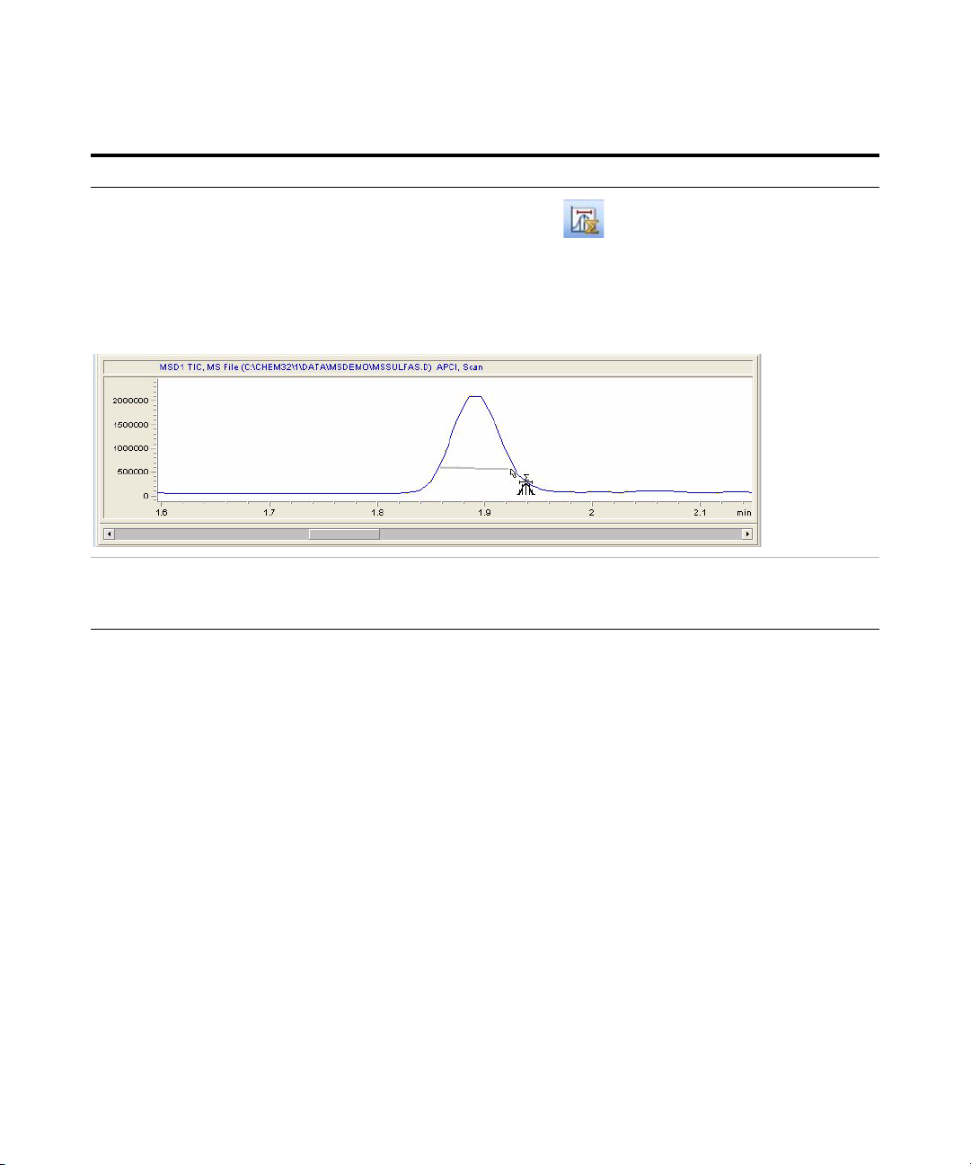
1 Display the total ion chromatogram in

its entirety.

2 Display the Integration Toolset. • Click the Integration

a Minimize any spectral windows that

hide the chromatogram window.

b Click the icon to zoom out.

icon, which is near the middle of the window.

36 Agilent 6100 Series Quadrupole LC/MS Systems Familiarization Guide

Qualitative Data Analysis 3

Exercise 3. Integrate the chromatogram

Steps Detailed Instructions Comments

3 Integrate the chromatogram. a Click the Auto Integrate

icon, which is near the middle of the window.

b Verify that the results are similar to

those shown below.

• Auto Integrate estimates initial integration parameters.

• If you do not see the retention times, in the graphics tools, click the icon to display retention times.

• If you do not see the pink integration baseline, in the graphics tools, click the icon to display baselines.

Agilent 6100 Series Quadrupole LC/MS Systems Familiarization Guide 37

3 Qualitative Data Analysis

Exercise 3. Integrate the chromatogram

Steps Detailed Instructions Comments

4 Adjust the integration parameters to

get only four integrated peaks.

a Click the icon for Edit/Set

Integration Events Table.

b In the Integration Events

table, for Baseline Correction, select Advanced.

c For Height Reject, type 500000. d Click the Integrate current

Chromatogram icon.

e Verify that your results are

similar to those shown below.

• For detailed information about integration events, see Agilent

ChemStation: Understanding Your ChemStation.

38 Agilent 6100 Series Quadrupole LC/MS Systems Familiarization Guide

Qualitative Data Analysis 3

Exercise 3. Integrate the chromatogram

Steps Detailed Instructions Comments

5 Save the integration events to the

method in memory.

6 Use the integrated chromatogram as

the basis for a faster way to display background-subtracted spectra.

• Click the icon to exit and save the integration results.

a Click the Spectrum

icon.

b Click the icon to display the

Spectral Options dialog box.

c Click the MS Reference tab. d Under Reference Spectrum, click

Automatic. e Click OK. f Click the icon to get a mass

spectrum at the peak apex. g In the chromatogram

window, click somewhere on the

fourth peak to get the spectrum. h Verify that the spectrum is similar to

the one shown below.

• To save the events to the method on disk, you also need to save the method to disk, as described in

step 3 on page 41.

• When you set Reference Spectrum, to Automatic, the software automatically takes the reference spectra for each peak, as described in the Spectral Options dialog box.

• The icon to get the mass spectrum at the peak apex is available only if you have integrated the chromatogram. No matter where you click on the peak, it gets the spectrum at the apex. With this tool, you may not need to zoom in on the chromatogram to achieve a precise location for the spectrum.

Agilent 6100 Series Quadrupole LC/MS Systems Familiarization Guide 39

3 Qualitative Data Analysis

Exercise 4. Print a report

In this exercise, you print a report, which you will use in

Chapter 4, “Set Up and Run a SIM Method.”

Steps Detailed Instructions Comments

1 Specify the LCMS Qualitative report

style, with the report printed to the screen.

a Select Report > Specify Report. b In the Specify Report dialog box,

under Destination, mark the check box for Screen.

c For Report Style, select LCMS

Qualitative.

d Check that other settings are as

shown below.

e Click OK.

40 Agilent 6100 Series Quadrupole LC/MS Systems Familiarization Guide

Qualitative Data Analysis 3

Exercise 4. Print a report

Steps Detailed Instructions Comments

2 Print the report. a Select Report > Print Report.

b After a short wait, view the Report

window.

c Verify that page 1 of the report

contains header information and an integrated chromatogram.

d At the bottom of the report window,

click the Next button.

e Verify that page 2 of the report

shows extracted ion chromatograms and a mass spectrum of the first chromatographic peak.

f Continue to click the Next button to

view results for the three additional chromatographic peaks.

g At the bottom of the report window,

click the Print button. This prints a hard copy of the report.

h At the bottom of the report window,

click the Close button.

3 Save the method. a Select File > Save > Method to

overwrite the method

SULFA MS SCAN 1.M.

b In the box for Comment for method

history, type a comment.

c Click OK.

• If you wish to complete Chapter 4,

“Set Up and Run a SIM Method”, then save the hard copy and refer to it when you set up your SIM groups.

• The extracted ion chromatograms are indicators of peak purity; if the retention times fail to coincide, the peak likely represents more than one compound.

• You save the method now so that your integration parameters, spectral display options, report settings, and other data analysis settings become part of the method.

Agilent 6100 Series Quadrupole LC/MS Systems Familiarization Guide 41

3 Qualitative Data Analysis

Exercise 4. Print a report

42 Agilent 6100 Series Quadrupole LC/MS Systems Familiarization Guide

Agilent 6100 Series Quadrupole LC/MS System Familiarization Guide

4 Set Up and Run a SIM Method

Exercise 1. Set up a SIM acquisition method 44

Task 1. Load the scan method you created previously 44 Task 2. Enter MS acquisition parameters 45

Exercise 2. Acquire data with the SIM method 48

Task 1. Enter sample information 49 Task 2. Acquire the data 50

These exercises show you how to set up a data acquisition method that uses selected ion monitoring (SIM). You set up the method for the demonstration sample (sulfa mix) and then run the sample with that method.

To set up the SIM method, you modify the scan method that you created in Chapter 2. To set up the SIM acquisition, you need the following for each of the four sulfa compounds:

• The LC retention time

• The masses of ions in the spectrum

You get that information from the report you generated in

Chapter 3.

Before you start

• Complete the previous exercises in this manual.

Agilent Technologies

4 Set Up and Run a SIM Method

Exercise 1. Set up a SIM acquisition method

In this exercise, you start with your existing scan method and modify it for SIM analysis. You keep the same LC conditions and modify only the MS conditions. This exercise consists of the following tasks:

• “Task 1. Load the scan method you created previously” (below)

• “Task 2. Enter MS acquisition parameters” on page 45

Task 1. Load the scan method you created previously

Steps Detailed Instructions Comments

4 Display Method and Run Control

view.

5 Open the method

SULFAMSSCAN1.M.

6 Save the method under a new name,

SULFA MS SIM 1.M.

• In the view selection area of the

ChemStation window, click Method and Run Control.

a Select File > Load > Method. b If necessary, navigate to

C:\CHEM32\1\METHODS.

c Select SULFA MS SCAN 1.M and

click OK.

a Select File > Save As > Method. b In the dialog box, for Name, type

SULFA MS SIM 1.M.

c Click OK. d In the box for Comment for method

history, type a comment.

e Click OK.

• You save the method now to avoid

inadvertent overwrites of your scan method.

44 Agilent 6100 Series Quadrupole LC/MS Systems Familiarization Guide

Set Up and Run a SIM Method 4

Task 2. Enter MS acquisition parameters

Steps Detailed Instructions Comments

1 Enter the chromatographic peak

width for the SIM analysis.

a Right-click the MSD

icon on the system diagram and select Set

up MSD Signals.

b When the Set Up MSD Signals

dialog box is displayed, type 0.05 For Peakwidth.

c Click OK.

• The peak width is an important

setting. It is used to calculate the appropriate SIM dwell times to deliver sufficient points across a chromatographic peak to give good quantitation.

• Peak width is defined as the full width at half maximum (FWHM), the width at 50% of the peak height.

Agilent 6100 Series Quadrupole LC/MS Systems Familiarization Guide 45

4 Set Up and Run a SIM Method

Task 2. Enter MS acquisition parameters

Steps Detailed Instructions Comments

2 Set up the first SIM ions using the

masses (to the nearest 0.1) that you observed in the spectra from your scan analysis:

• Sulfamethizole: Time 0,

SIM Ions 271 and 156.

a Under MSD Signal Settings, Signal

1, for Mode, select SIM.

b In the table, for Fragmentor, type

one of the following:

• 150 for the Agilent 6120

• 200 for the Agilent 6130 or 6150

c In the table, change Group 1 to

Sulfamethizole, and for SIM Ion,

refer to the spectrum on your printout and type the mass (to the nearest 0.1) for the 271 ion.

d Click Add Ion, and type the mass for

the sulfamethizole 156 ion.

• In this example, each SIM group includes a pseudo-molecular ion and one fragment ion for confirmation.

• Note that the figure below does not show the fourth sulfa drug.

46 Agilent 6100 Series Quadrupole LC/MS Systems Familiarization Guide

Set Up and Run a SIM Method 4

Task 2. Enter MS acquisition parameters

Steps Detailed Instructions Comments

3 Set up the remaining SIM ions, using

the masses (to the nearest 0.1) that you observed in the spectra from your scan analysis:

• Sulfachloropyridazine: Time 1.3,

SIM Ions 285, 287, and 156.

• Sulfamethazine: Time 2.3,

SIM Ions 279 and 186.

• Sulfadimethoxine: Time 3.3,

SIM Ions 311 and 156.

4 Save the method. a Select Method > Save Method to

a Click Add Grp, and type the name,

start time and mass (approximately

285) for sulfachloropyridazine.

b Click Add Ion, and type the mass for

the sulfachloropyridazine 156 ion.

c Click Add Ion, and type the mass for

the sulfachloropyridazine 287 ion.

d Repeat these steps until you have

entered two or three ions for each of the remaining compounds.

e Click OK to close the Set Up MSD

Signals dialog box.

overwrite the method

SULFA MS SIM 1.M.

b In the box for Comment for method

history, type a comment.

c Click OK.

• Alternatively, instead of making

separate groups for each compound as described here, all of the SIM ions could be entered into “Group 1", which could be re-named “Sulfonamides”. The first SIM group can contain up to 100 ions.

• You may need to adjust the start time for each SIM group. Refer to your printout from Chapter 3 to determine a start time so that each group change occurs about midway between the chromatographic peaks.

• If the retention time difference between sulfachloropyridazine and sulfamethazine is less than 0.3 minutes, merge these ions into one group.

• The sulfachloropyridazine additionally includes the chlorine isotope at m/z 287.

Agilent 6100 Series Quadrupole LC/MS Systems Familiarization Guide 47

4 Set Up and Run a SIM Method

Exercise 2. Acquire data with the SIM method

Now you are ready to acquire data for the sulfa mix with the method you just created. This exercise consists of the following tasks:

• “Task 1. Enter sample information” on page 49

• “Task 2. Acquire the data” on page 50

48 Agilent 6100 Series Quadrupole LC/MS Systems Familiarization Guide

Set Up and Run a SIM Method 4

Task 1. Enter sample information

Steps Detailed Instructions Comments

1 Display the Single Sample toolbar. • In the top toolbar, click

the single sample icon.

1 Display the Sample Information dialog

box.

2 Enter the sample information:

• Operator name

• Subdirectory: Sulfas

• Prefix: Sulfa_SIM

• Location: Vial 1

• Sample Name: Sulfas 10 ng/µL

• Comment: SIM familiarization

exercise

a Click Sample Info on the

RunControl menu.

a Enter the parameters described in

step 2 and shown in the figure

below.

b Click OK.

• If you select Prefix/Counter, the

file names increment automatically from one run to the next.

Agilent 6100 Series Quadrupole LC/MS Systems Familiarization Guide 49

4 Set Up and Run a SIM Method

Task 2. Acquire the data

Steps Detailed Instructions Comments

1 Place the vial of sulfa sample you

prepared at 10 ng/µL into position 1 in the autosampler.

2 Inject the sulfa mix sample. • Click the Single Sample start

button.

3 Monitor the total ion chromatogram

and the UV chromatogram during data acquisition.

4 When the analysis is done, view the

results.

a Activate the Online Plot window. b Monitor the MS signal to ensure a

stable baseline.

a Display Data Analysis view. b Load the data file you just created. c Examine the DAD and MS

chromatograms.

• You prepared this sample in

“Exercise 2. Prepare the samples for the analyses” on page 12.

This button is present only when you have selected Single Sample mode from the top toolbar.

• If the baseline fluctuation for the MS signal is greater than 10%, the nebulizer and source chamber may require maintenance. See the

Agilent 6100 Series Single Quad LC/MS System Maintenance Guide.

• If you need help, follow the general procedure in “Exercise 1. Display

and manipulate chromatograms” on

page 28 in Chapter 3.

50 Agilent 6100 Series Quadrupole LC/MS Systems Familiarization Guide

Agilent 6100 Series Quadrupole LC/MS System Familiarization Guide

5 Set Up and Run a Sequence

Exercise 1. Set up a sequence 52

Task 1. Prepare to create a new sequence 52 Task 2. Edit sequence parameters 53 Task 3. Set up the sequence table 55 Task 4. Set up the sequence output 58

Exercise 2. Run the sequence 60

These exercises show you how to set up a sequence for the SIM analysis of the demonstration sample (sulfa mix), and to acquire data with that sequence.

In the sequence, you run the sulfa mix at three concentrations: 1, 5 and 10 ng/µL. You also run a solvent blank.

Before you start

• Read the Agilent 6100 Series Quadrupole LC/MS Systems Quick Start Guide and Chapter 3 of the Agilent 6100 Series Quadrupole LC/MS Systems Concepts Guide.

• Complete the previous exercises in this manual.

For details about sequences, see the automation chapter in Agilent ChemStation: Understanding Your ChemStation.

Agilent Technologies

5 Set Up and Run a Sequence

Exercise 1. Set up a sequence

Task 1. Prepare to create a new sequence

Steps Detailed Instructions Comments

1 Display Method and Run Control

view.

2 Display the Sequence Toolset. • In the top toolbar, click

3 Display the Autosampler Tray

diagram.

• In the view selection area of the

ChemStation window, click Method and Run Control.

the icon to display the

Sequence Toolset.

• Click Sampling Diagram on the View menu.

4 Initiate setup of a new sequence. • Select Sequence> New sequence. The empty default sequence file,

DEF_LC.S, is loaded automatically.

5 Save the sequence under a new

name, SULFA MS SIM 1.S

a Select Sequence > Save Sequence As. b For Name, type SULFA MS SIM 1.S. c Click OK.

52 Agilent 6100 Series Quadrupole LC/MS Systems Familiarization Guide

Set Up and Run a Sequence 5

Task 2. Edit sequence parameters

Steps Detailed Instructions Comments

1 Open Sequence Parameters dialog

box.

2 Enter the sequence parameters for

Operator Name and Data File.

• Click Sequence > Sequence

Parameters.

a Enter the following parameters,

shown in step 1.

• Operator name: You r na m e

• Subdirectory: Sulfas

• Prefix: Sulfa_seq

• The sequence parameters are

settings that are common to all the samples in the sequence.

• To avoid overwrite of data files, type a new subdirectory for each sequence. The directory will be created if it doesn’t already exist on your computer.

• Unique file names are automatically created for each data file within the subdirectory.

Agilent 6100 Series Quadrupole LC/MS Systems Familiarization Guide 53

5 Set Up and Run a Sequence

Task 2. Edit sequence parameters

Steps Detailed Instructions Comments

3 Enter the rest of the sequence

parameters:

a Enter the following parameters

shown in the figure below.

• Parts of methods to run:

According to Runtime Checklist

• Wait: 10 minutes after loading a

new method

• Shutdown: STANDBY

• Not Ready Timeout: 15 minutes

• Sequence Comment: Sequence

familiarization exercise

b Click OK.

• If you wanted to run only

reprocessing (data analysis), you would set that in Part of methods to

run.

• The Wait allows the instrument to

equilibrate when a new method is loaded.

Post-Sequence Command/Macros are a convenient way to turn off lamps, pumps, etc. The command or macro is run at the end of the sequence or in the event of an error.

Two examples of Post-Sequence Command/Macros are:

• MSSetState is a command that can change the MS state to standby. See the online Help for commands.

• SHUTDOWN.MAC is a macro that will shut down the system, but you must customize it before using it.

54 Agilent 6100 Series Quadrupole LC/MS Systems Familiarization Guide

Set Up and Run a Sequence 5

Task 3. Set up the sequence table

Steps Detailed Instructions Comments

1 Set up the sequence table to:

• Run duplicate injections of a blank.

• Run duplicate injections of the

sulfa mix at three concentrations: 1, 5 and 10 ng/µL.

• Use the method

SULFA MS SIM 1.M, that you

created in Chapter 4, “Set Up and Run a SIM Method”.

a Click Sequence > Sequence Table. b Select the first line of the sequence

table. In the sequence table, under

Line, click the number 1.

c Click the Cut button to delete the

line.

d Click the button for the

Insert/Filldown Wizard, shown

below.

e Fill in the values and click OK.

• In this step, you set up the parts of

the sequence table that are common to all the samples.

• You will specify the sample names later in this exercise.

• There are a number of ways to add samples to the sequence table. This exercise illustrates just one of the ways — use of the Insert/Filldown

Wizard.

Agilent 6100 Series Quadrupole LC/MS Systems Familiarization Guide 55

5 Set Up and Run a Sequence

Task 3. Set up the sequence table

Steps Detailed Instructions Comments

2 View the sequence table that you

have created so far.

3 (Optional) Customize the sequence

table to match the format in step 2.

a Compare your table with the one

below.

b Note any differences, such as

columns that are included and column widths.

a In the lower right-hand

corner of the dialog box, click the icon to customize the sequence table.

b Clear the check boxes for any

unnecessary columns, as shown below.

c Increase the width of the column for

the sample name, as shown below.

d Decrease the width of the column

for the method name, as shown below.

e Click OK.

• Your results will likely differ, but in

the next step you may recreate the table format below.

• For descriptions of any columns you removed, see the online Help.

56 Agilent 6100 Series Quadrupole LC/MS Systems Familiarization Guide

Set Up and Run a Sequence 5

Task 3. Set up the sequence table

Steps Detailed Instructions Comments

4 Type the following sample names into

the table:

• Vial 1 – blank

• Remaining vials – sulfa mix at 1, 5

and 10 ng/µL

5 Save the sequence. • Click the Save Sequence

a Modify the Sample Name for each

sample, as shown below.

b Click OK.

button in the Sequence toolset.

Agilent 6100 Series Quadrupole LC/MS Systems Familiarization Guide 57

5 Set Up and Run a Sequence

Task 4. Set up the sequence output

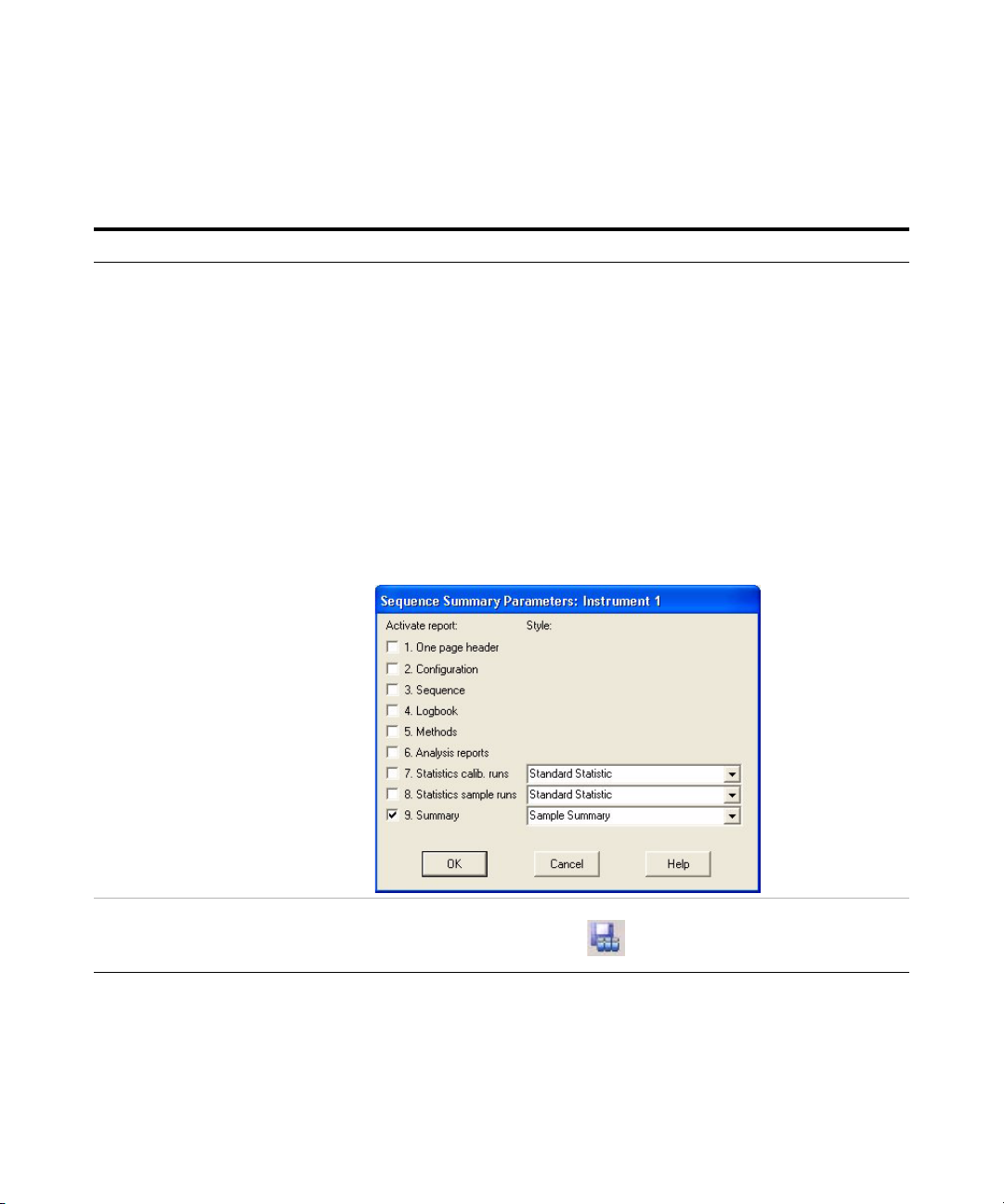
Steps Detailed Instructions Comments

1 Set up the sequence to print a short

sequence summary to the printer.

a Click Sequence > Sequence

Output.

b Mark the check box for Print

Sequence Summary Report.

c Mark the check box for Report to

Printer. d Click the Setup button. e Fill in the dialog box as shown

below. f Click OK in the Sequence Summary

Parameters dialog box. g Click OK in the Sequence Output

dialog box.

• In addition to the sequence summary report, you can print individual sample reports, as specified in your method. (You do not print individual reports in this exercise.)

• For details about sequence reports, see the chapter on ChemStation reports in Agilent ChemStation: Understanding Your ChemStation.

• The setup shown in the dialog box below prints the simplest summary report.

2 Save the sequence. • Click the Save Sequence

button in the Sequence toolset.

58 Agilent 6100 Series Quadrupole LC/MS Systems Familiarization Guide

Set Up and Run a Sequence 5

Task 4. Set up the sequence output

Steps Detailed Instructions Comments

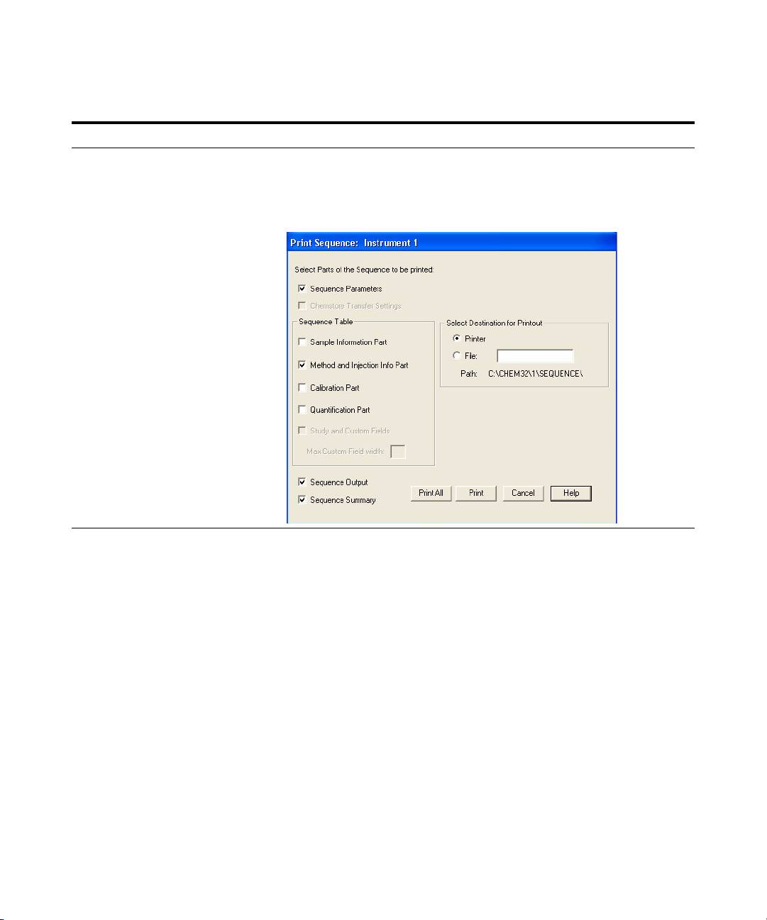
3 Print the sequence. a Select Sequence > Print Sequence.

b Mark the check boxes as shown in

the figure below.

c Click the Print button.

If you click the Print All button, you print all the parts of the sequence rather than the items you just specified.

Agilent 6100 Series Quadrupole LC/MS Systems Familiarization Guide 59

5 Set Up and Run a Sequence

Exercise 2. Run the sequence

Now you are ready to acquire data with the sequence you just created.

Steps Detailed Instructions Comments

1 Confirm that your sequence includes

four samples.

2 Place the samples you prepared in

Chapter 1 into the appropriate

positions in the autosampler.

3 Inject the samples. • Click the Sequence

4 (Optional) For the first blank analysis,

monitor the total ion chromatogram and the UV chromatogram during data acquisition.

5 When the sequence is done, view the

Sequence Summary Report.

6 When the sequence is finished, view

the results.

• Verify that the Autosampler Tray diagram shows four samples.

start button on the Run Control Bar.

a Activate the Online Plot window. b Monitor the MS signal to ensure a

stable baseline.

a Retrieve the report from the printer. b Examine the report to confirm that

all the samples ran.

a Display Data Analysis view. b Load the first data file you just

created.

c Examine the DAD and MS

chromatograms.

d Repeat step b and step c for the

other data files.

You prepared the samples in “Exercise

2. Prepare the samples for the analyses” on page 12.

This button is only available if you have selected Sequence mode on the main toolbar.

As the sequence progresses, the Autosampler Tray diagram is color-coded as follows:

Gray - samples that have been analyzed.

White - samples not yet analyzed.

Blue - the current sample.

• If you need help, follow the general procedure in “Exercise 1. Display

and manipulate chromatograms” on

page 28 in Chapter 3.

• When you analyze your own samples, you can set up your method to automatically generate a data analysis report for each sample in the sequence.

60 Agilent 6100 Series Quadrupole LC/MS Systems Familiarization Guide

Agilent 6100 Series Quadrupole LC/MS System Familiarization Guide

6 Quantitative Data Analysis

Exercise 1. Create a method for quantification 62

Exercise 2. Process a sample and print a report 73

This chapter shows you how to use the ChemStation Data Analysis to perform quantification. The exercises in this chapter illustrate a simple calibration that uses data files that you received with your ChemStation software.

Before you start

• Read the Agilent 6100 Series Quadrupole LC/MS Systems Quick Start Guide.

• Read the chapter on Data Analysis in the Agilent 6100 Series Quadrupole LC/MS Systems Concepts Guide.

• Make sure that you have the caffeine data files on your ChemStation. Check for the files under

C:\CHEM32\1\DATA\MSDEMO. The file names are CAFCAL0X.D, where x is a number from 1 to 5.

Agilent Technologies

6 Quantitative Data Analysis

Exercise 1. Create a method for quantification

In this exercise, you create a calibrated method that you can use to quantify caffeine in the demo data.

Task 1. Create a new method

In this task, you load a default method and save it to a new name. You later modify the new method to create a calibrated method.

Steps Detailed Instructions Comments

1 Display Data Analysis view. • In the view selection area in the

lower left of the ChemStation window, click Data Analysis.

2 Load the method DEF_LC.M. a Click File > Load > Method.

b Navigate to the folder

C:\CHEM32\1\METHODS.

c Select the method file and click OK.

3 Save the method under the new name

CAFFEINE CAL.M.

a Select File > Save As > Method. b Navigate to the folder

C:\CHEM32\1\METHODS.

c In the dialog box, for Name, type

CAFFEINE CAL.M.

d Click OK. e In the box for Comment for method

history, type a comment.

f Click OK.

62 Agilent 6100 Series Quadrupole LC/MS Systems Familiarization Guide

Quantitative Data Analysis 6

Task 2. Set up the signal for quantification

In this exercise, you add an extracted ion chromatogram (EIC) to the list of available signals for the method. Then you add this EIC to the Signal Details, so you can automatically load and integrate signals for the rest of the caffeine standards.

Steps Detailed Instructions Comments

1 Open the data file CAFCAL01.D,

located in the MSDEMO folder.

2 Extract the major ion of caffeine. a Select File > Extract Ions.

3 Display the Calibration Toolset. • Click the Calibration

a Select File > Load Signal. b Navigate to the folder:

C:\CHEM32\1\DATA\MSDEMO. c Select the data file CAFCAL01.D. d If necessary, clear the check box for

Load using Signal Details. e In the Signals box, click the signal

that begins with MSD1 TIC. f Click OK.

b For Ion 1, type 195.1. c For Ion 2, type 195.1. d Click OK.

icon, which is near the middle of the window.

• For other ways to load signals, see the chapter on Data Analysis in the Concepts Guide.

• The 195 ion is the (M+H)

ion.

Agilent 6100 Series Quadrupole LC/MS Systems Familiarization Guide 63

6 Quantitative Data Analysis

Task 2. Set up the signal for quantification

Steps Detailed Instructions Comments

4 Set up the signal for quantification. a Do one of the following:

• Click the icon to Edit

current method signals.

• Select Calibration >

Signal Details.

b From the list of Available Signals,

select MSD1 195, EIC=195.1:195.1. c Click Add to Method. d Click OK.

5 (Optional) Save the method under the

same name (CAFFEINE CAL.M).

a Select File > Save > Method. b In the box for Comment for method

history, type a comment. c Click OK.

• The EIC signal is available only

because you loaded the 195 EIC in

step 2.

• For these exercises, you save the method frequently, but you could wait instead until you had established all the method settings.

64 Agilent 6100 Series Quadrupole LC/MS Systems Familiarization Guide

Quantitative Data Analysis 6

Task 3. Integrate the low-level standard

In this exercise, you establish integration parameters for your calibrated method. You use the low-level standard because it is usually the most difficult to integrate.

Steps Detailed Instructions Comments

1 Display the Integration Toolset. • Click the

Integration icon,

which is near the middle of the window.

2 Integrate the chromatogram. a Click the Auto Integrate

icon, which is near the middle of the window.

b Check that you have five integrated

peaks with these initial settings.

• Auto Integrate estimates initial integration parameters and then performs the integration.

Agilent 6100 Series Quadrupole LC/MS Systems Familiarization Guide 65

6 Quantitative Data Analysis

Task 3. Integrate the low-level standard

Steps Detailed Instructions Comments

3 Adjust the integration parameters to

get one integrated peak.

a Click the icon to Edit/Set

Integration Events Table.

b In the integration events for

all signals, for Baseline Correction, select Advanced.

c Click the Auto Integrate

icon.

d When you are prompted to

save the events table, click Yes .

e Verify that your results are the same

or very similar to those shown below.

• For detailed information about integration events, see Agilent

ChemStation: Understanding Your ChemStation.

4 Save the integration events with the

method in memory.

5 (Optional) Save the method under the

same name (CAFFEINE CAL.M).

• Click the icon to exit and save the integration results.

a Select File > Save > Method. b In the box for Comment for method

history, type a comment.

c Click OK.

66 Agilent 6100 Series Quadrupole LC/MS Systems Familiarization Guide

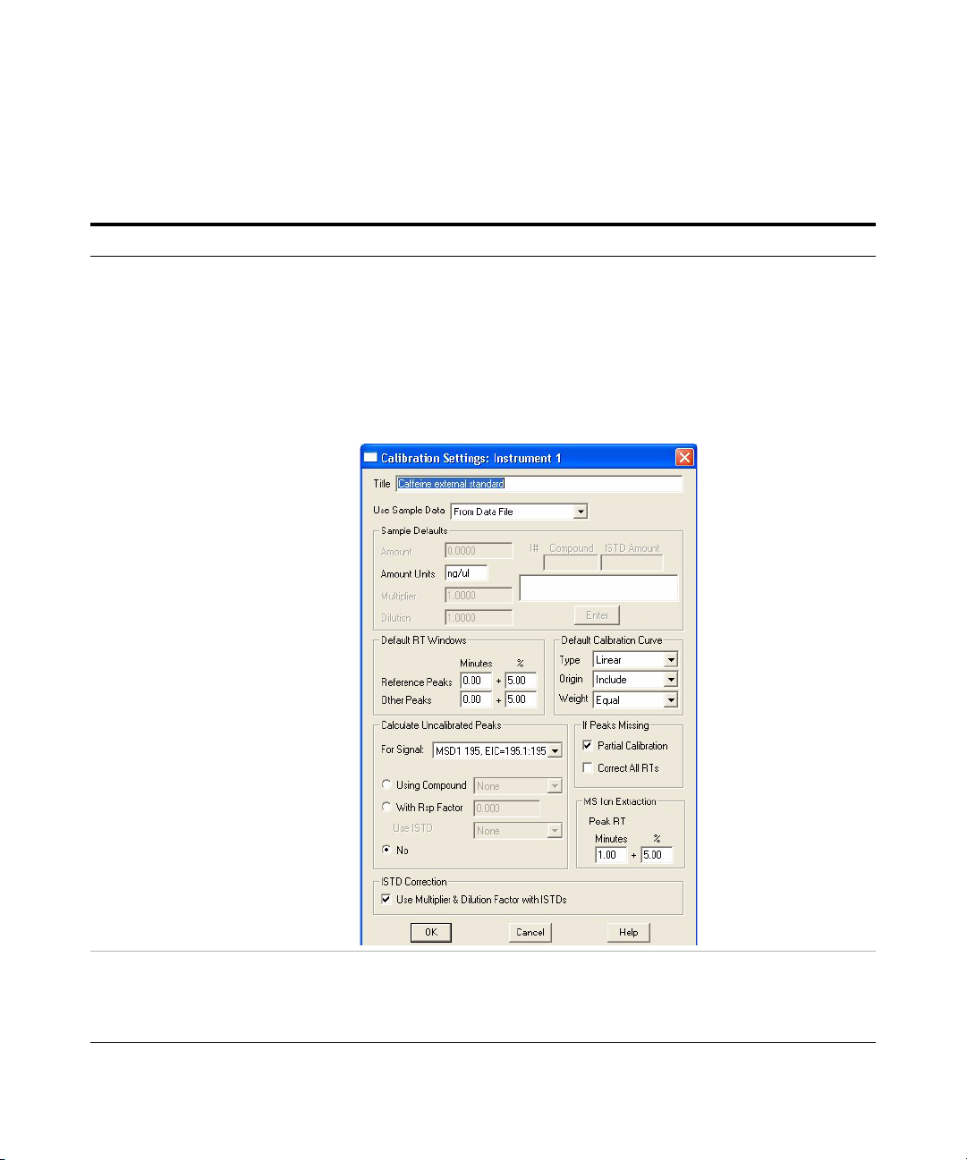
Quantitative Data Analysis 6

Task 4. Set general calibration parameters

Steps Detailed Instructions Comments

1 Establish calibration parameters. a Select Calibration > Calibration

Settings.

b In the Title box, type a title, for

example Caffeine external standard.

c Leave the rest of the items at the

default settings, shown below.

d Click OK.

2 (Optional) Save the method under the

same name (CAFFEINE CAL.M).

a Select File > Save > Method. b In the box for Comment for method

history, type a comment.

c Click OK.

Agilent 6100 Series Quadrupole LC/MS Systems Familiarization Guide 67

6 Quantitative Data Analysis

Task 5. Set up the calibration curve

In this exercise, you integrate the rest of the standards and add all standards to the calibration curve.

Steps Detailed Instructions Comments

1 Display the Calibration Toolset. • Click the Calibration

icon, which is near the middle of the window.

2 Add the low-level standard to the

calibration curve.

a Do one of the following:

• Click the New

Calibration Table icon.

• Select Calibration >

New Calibration Table. b Click Automatic Setup Level 1. c Click OK. d In the Calibration Table pane

(shown below), under Compound, type caffeine and under Amt (amount), type 0.5.

• Do not worry at this point if your calibration curve displays a message that says the curve is invalid.

68 Agilent 6100 Series Quadrupole LC/MS Systems Familiarization Guide

Quantitative Data Analysis 6

Task 5. Set up the calibration curve

Steps Detailed Instructions Comments

3 Load and integrate the second

standard.

a Select File > Load Signal. b Under File name, select

CAFCAL02.D.

c Mark the check box for Load using

Signal Details.

d Mark the check box for Integrate

after load.

e Check that your dialog box looks like

the one below.

f Click OK.

• These settings enable you in a

single step to load the appropriate signal(s) and integrate them.

4 Add the second standard to the

calibration curve.

a Click the icon to Add new

level.

b In the dialog box, for

Default Amount, type 1 and click OK.

c Verify that the calibration table now

has two entries, and the calibration curve contains two points.

Agilent 6100 Series Quadrupole LC/MS Systems Familiarization Guide 69

6 Quantitative Data Analysis

Task 5. Set up the calibration curve

Steps Detailed Instructions Comments

5 Add the remaining three standards to

the calibration table:

• CAFCAL03.D: 5 ng/µL

• CAFCAL04.D: 25 ng/µL

• CAFCAL05.D: 50 ng/µL

a Select File > Load Signal. b Under File name, select the next

data file.

c Verify that the chromatogram is

properly integrated.

d Click the icon to Add new

level.

e In the dialog box, for

Default Amount, type the amount shown in step 5 and click OK.

f Verify that the calibration table and

the calibration curve contain the new entry.

g Repeat step a through step f until

you have added all the standards.

h Confirm that your calibration table

and calibration curve look like the ones below.

• If multiple peaks are integrated in a chromatogram, retention time is used to find the correct peak for the calibration curve.

70 Agilent 6100 Series Quadrupole LC/MS Systems Familiarization Guide

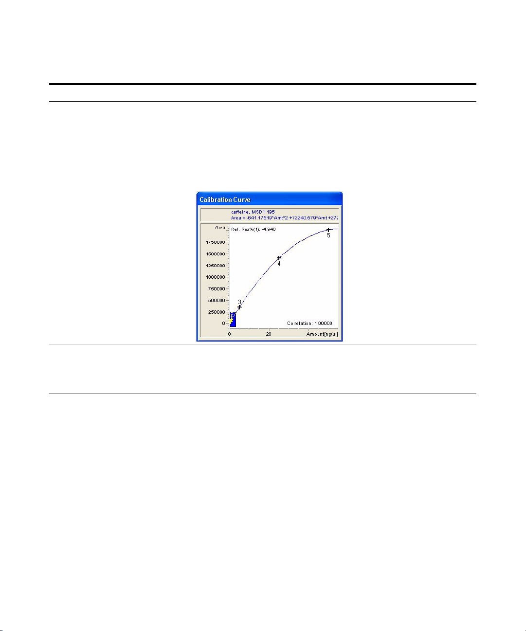
Quantitative Data Analysis 6

Task 5. Set up the calibration curve

Steps Detailed Instructions Comments

6 Refine the calibration curve. a Select Calibration > Calibration

Settings.

b Under Default Calibration Curve,

for Ty p e , select Quadratic. c Click OK. d Verify that your calibration curve

now looks like the one below.

7 (Optional) Save the method under the

same name (CAFFEINE CAL.M).

a Select File > Save > Method. b In the box for Comment for method

history, type a comment. c Click OK.

Agilent 6100 Series Quadrupole LC/MS Systems Familiarization Guide 71

6 Quantitative Data Analysis

Task 6. Explore options to refine the calibration

This exercise describes additional calibration table layouts that give you more calibration options. You do not need these options to process the caffeine demonstration data, but you may need them when you process your own samples.

Steps Detailed Instructions Comments

1 Explore options to change the way

calibration curves are constructed.

2 Explore options to add qualifier ions. a Select Calibration Table Options >

3 Display the original options for the

calibration table.

a Select Calibration Table Options >

Peak Details. b Verif y that you see these columns in

the calibration table:

• Curve Type

• Origin

• Weight

Identification Details. b Verif y that you see these columns in

the calibration table:

• Resp % (response percent)

• +- (window for the response

percent)

• Pk Usage (peak usage)

a Select Calibration Table Options >

Overview. b Verify that the calibration table

looks the same as in step 5 on

page 70.

• Note that this calibration table layout lets you change:

• Curve Type: The type of

calibration curve (linear, quadratic, etc.)

• Origin: How the origin (zero

point) is treated.

• Weight: The relative weights of

the data points.

• Note that this calibration table layout lets you define:

• Pk Usage: How the calibration

uses the peak, for example, as a main calibration ion or a qualifier ion

• Resp %: The expected response

of the qualifier ion, as a percentage of the main peak

• +-: A window for the expected

percentage.

72 Agilent 6100 Series Quadrupole LC/MS Systems Familiarization Guide

Quantitative Data Analysis 6

Exercise 2. Process a sample and print a report

In this exercise, you specify a report and test your calibration method by processing one of the standards as if it were a sample. You print a report of the results.

Steps Detailed Instructions Comments

1 Specify a report with the following

settings:

• Report destination: Screen

• External standard (ESTD)

calculation, based on area

• Report style: Detail

a Do one of the following:

• Select Report > Specify Report.

• Click the Specify Report

icon.

b Enter parameters as

described in step 1 and shown in the figure below.

c Click OK.

Agilent 6100 Series Quadrupole LC/MS Systems Familiarization Guide 73

6 Quantitative Data Analysis

Exercise 2. Process a sample and print a report

Steps Detailed Instructions Comments

2 Save the method under the same

name (CAFFEINE CAL.M).

3 Load the standard of medium

concentration.

4 Process the medium-level standard

and print the report.

a Select File > Save > Method. b In the box for Comment for method

history, type a comment.

c Click OK.

a Select File > Load Signal. b Under File name, select

CAFCAL03.D.

a Do one of the following:

• Select Report > Print Report.

• Click the icon to preview

results.

b Verify that page 1 of the

report contains header information, an integrated chromatogram, and an external standard report.

c Check that the caffeine amount is

about 5 ng/µL.

d At the bottom of the report window,

click the Next button.

e Verify that page 2 of the report

shows the calibration curve with the measured point identified with dotted lines.

f (Optional) At the bottom of the

report window, click the Print button so you get a hard copy.

g At the bottom of the report window,

click the Close button.

• Another way to generate a hard copy is to click the

Print Report icon.

74 Agilent 6100 Series Quadrupole LC/MS Systems Familiarization Guide

www.agilent.com

In This Book

When you do the exercises in this book, you learn how to:

• Prepare your LC/MS system for an analysis

•Set up methods for scan and selected ion monitoring analyses

•Acquire data

• Set up sequences for automated sample analyses

• Perform qualitative and quantitative analyses.

Printed in USA Revision A, September 2011

*G1960-90080*

G1960-90080

Agilent Technologies

Agilent 6100 Familiarization Guide

Specifications and Main Features

Frequently Asked Questions

User Manual