Agilent 54621D Programmer’s Guide

Download

Programmer’s Guide

Publication Number 54622-97001 May 2000

For Safety information, Warranties, and Regulatory information, see the pages behind the Index.

54621A/22A/24A Oscilloscopes and 54621D/22D Mixed-Signal Oscilloscopes

Programming the Oscilloscope

When you attach an interface module to the rear of the oscilloscope, it becomes programmable. That is, you can hook a controller (such as a PC or workstation) to it, and write programs on that controller to automate oscilloscope setup and data capture.

The following figure shows the basic structure of every program you will write for the oscilloscope.

Initialize

To ensure consistent, repeatable performance, you need to start the program, controller, and oscilloscope in a known state. Without correct initialization, your program may run correctly in one instance and not in another. This might be due to changes made in configuration by previous program runs or from the front panel of the oscilloscope.

• Program initialization defines and initializes variables, allocates memory, or tests system configuration.

• Controller initialization ensures that the interface to the oscilloscope (either GPIB or RS-232) is properly set up and ready for data transfer.

• Oscilloscope initialization sets the channel configuration and labels, threshold voltages, trigger specification and mode, timebase, and acquisition type.

Capture

Once you initialize the oscilloscope, you can begin capturing data for analysis. Remember that while the oscilloscope is responding to commands from the controller, it is not performing acquisitions. Also, when you change the oscilloscope configuration, any data already captured will most likely be rendered.

To collect data, you use the :DIGitize command. This command clears the waveform buffers and starts the acquisition process. Acquisition continues until acquisition memory is full, then stops. The acquired data is displayed by the oscilloscope, and the captured data can be measured, stored in trace memory in the oscilloscope, or transferred to the controller for further analysis. Any additional commands sent while :DIGitize is working are buffered until :DIGitize is complete.

You could also put the oscilloscope into run mode, then use a wait loop in your program to ensure that the oscilloscope has completed at least one acquisition before you make a measurement. HP does not recommend this because the needed length of the wait loop may vary, causing your program to fail. :DIGitize, on the other hand, ensures that data capture is complete. Also, :DIGitize, when complete, stops the acquisition process so that all measurements are on displayed data, not on a constantly changing data set.

Analyze

After the oscilloscope has completed an acquisition, you can find out more about the data, either by using the oscilloscope measurements or by transferring the data to the controller for manipulation by your program. Built-in measurements include frequency, duty cycle, period, and positive and negative pulse width.

Using the :WAVeform commands, you can transfer the data to your contro l ler. You may wa nt t o d isplay the da t a, c ompar e it to a known good measurement, or simply check logic patterns at various time intervals in the acquisition.

iii

In This Book

This Programmer’s Guide is your introduction to programming the oscilloscope using an instrument controller. This book, with the Programmer’s Reference, provides a comprehensive description of the oscilloscope’s programmatic interface. The Programmer’s Reference is supplied as a Microsoft Windows Help file on a 3.5" diskette.

The oscilloscope has a built-in RS-232-C port for programming. To program the oscilloscope over GP-IB, you need the N2757A GPIB Interface Module. You also need an instrument controller that supports either the IEEE-488 or RS-232-C interface standards, and a programming language capable of communicating with these interfaces.

This book contains the following information: Chapter 1 Introduction to Programming, gives a general overview of

oscilloscope programming. Chapter 2 Programming Getting Started, shows a simple program, explains

its operation, and discusses considerations for data types. Chapter 3 GPIB, discusses the general considerations for programming the

instrument over an GPIB interface. Chapter 4 P rogramming over RS-232-C, discus ses the general considerations

for programming the instrument over an RS-232-C interface. Chapter 5 Programming and Documentation Conventions, describes the

conven ti o ns use d in repr e s enting the syn t ax of com m ands throu gh out this book and the Programmer’s Reference, and gives an overview of the oscilloscope command set.

Chapter 6 Status Reporting, discusses the oscilloscope status registers and how to use them in your programs.

Chapter 7 Installing and Using the Programmer’s Reference, tells how to install the Programmer’s Reference online help file in Microsoft Windows, and explains help file navigation.

Chapter 8 Programmer’s Quick Reference, lists all the commands and queries available for programming the oscilloscope.

For information on oscilloscope operation, see the User’s Guide. For information on interface configuration, see the documentation for the oscilloscope interface module and the interface card used in your controller (for example, the HP82350A interface for IBM PC-compatible computers).

1 Introduction to Programming

Talking to the Instrument 1-3 Program Message Syntax 1-4 Combining Commands from the Same Subsystem 1-7 Duplicate Mnemonics 1-8 Query Command 1-9 Program Header Options 1-10 Program Data Syntax Rules 1-11 Program Message Terminator 1-13 Selecting Multiple Subsystems 1-14

2 Programming Getting Started

Initialization 2-3 Autoscale 2-4 Setting Up the Instrument 2-5 Example Program 2-6 Using the DIGitize Command 2-7 Receiving Information from the Instrument 2-9 String Variables 2-10 Numeric Variables 2-11 Definite-Length Block Response Data 2-12 Multiple Queries 2-13 Instrument Status 2-13

3 Programming over GPIB

Interface Capabilities 3-3 Command and Data Concepts 3-3 Addressing 3-4 Communicating Over the Bus 3-5 Lockout 3-6 Bus Commands 3-6

4 Programming over RS-232-C

Interface Operation 4-3 Cables 4-3 Minimum Three-Wire Interface with Software Protocol 4-4 Extended Interface with Hardware Handshake 4-5 Configuring the Interface 4-7 Interface Capabilities 4-7 Communicating Over the RS-232-C Bus 4-8

Contents-1

Contents

5 Programming and Documentation Conventions

Command Set Organization 5-3 The Command Tree 5-6 Obsolete and Discontinued Commands 5-10 Truncation Rules 5-14 Infinity Representation 5-15 Sequential and Overlapped Commands 5-15 Response Generation 5-15 Notation Conventions and Definitions 5-16 Program Examples 5-17

6 Status Reporting

Status Reporting Data Structures 6-5 Status Byte Register (SBR) 6-8 Service Request Enable Register (SRER) 6-10 Trigger Event Register (TRG) 6-10 Standard Event Status Register (SESR) 6-11 Standard Event Status Enable Register (SESER) 6-12 User Event Register (UER) 6-13 Local Event Register (LCL) 6-13 Operation Status Register (OPR) 6-13 Limit Test Event Register (LTER) 6-14 Mask Test Event Register (MTER) 6-15 Histogram Event Register (HER) 6-16 Arm Event Register (ARM) 6-16 Error Queue 6-17 Output Queue 6-18 Message Queue 6-18 Key Queue 6-18 Clearing Registers and Queues 6-18

7 Installing and Using the Programmer’s Reference

To install the help file under Microsoft Windows 7-3 To get updated help and program files via the Internet 7-4 To start the help file 7-5 To navigate through the help file 7-5

8 Programmer’s Quick Reference

Conventions 8-3 Suffix Multipliers 8-3 Commands and Queries 8-4

Contents-2

Introduction to Programming

Chapters 1 and 2 introduce the basics for remote programming of an oscilloscope. The programming instructions in this manual conform to the IEEE488.2 Standard Digital Interface for Programmable Instrumentation. The programming instructions provide the means of remote control.

To program the oscilloscope you must add either a GPIB (N2757A) interface, or program over the built-in RS-232-C interface on the rear panel.

You can perform the following basic operations with a controller and an oscilloscope:

• Set up the instrument.

• Make measurements.

• Acquire data (waveform, measurements, configuration) from the oscilloscope.

• Send information (pixel images, configurations) to the oscilloscope.

Other tasks are accomplished by combining these basic functions.

Languages for Program Examples

The programming examples for individual commands in this manual are written in HPBASIC 6.3 or C.

1-2

Introduction to Programming

Talking to the Instrument

Computers acting as controllers communicate with the instrument by sending and receiving messages over a remote interface. Instructions for programming normally appear as ASCII character strings embedded inside the output statements of a host language available on your controller. The input statements of the host language are used to read in responses from the oscilloscope.

For example, HPBASIC uses the OUTPUT statement for sending commands and queries. After a query is sent, the response is usually read in using the ENTER statement.

Messages are placed on the bus using an output command and passing the device address, program message, and terminator. Passing the device address ensures that the program message is sent to the correct interface and instrument.

The following HP BASIC statement sends a command which turns on label desplay.

OUTPUT < device address > ;":CHANNEL1:BWLIMIT ON"<terminator>

The < dev ice ad d r ess > rep r e sents t h e add ress o f the devi c e bei n g pr ogramme d . Each of the other parts of the above statement are explained in the following pages.

1-3

Figure 1-1

Introduction to Programming

Program Message Syntax

To program the instrument remotely, you must understand the command format and structure expected by the instrument. The IEEE 488.2 syntax rules govern how individual elements such as headers, separators, program data, and terminators may be grouped together to form complete instructions. Syntax definitions are also given to show how query responses are formatted. The following figure shows the main syntactical parts of a typical program statement.

Program Message Syntax

Output Command

The output command is entirely dependent on the programming language. Throughout this manual, HPBASIC is used in most examples of individual commands. If you are using other languages, you will need to find the equivalents of HP BASIC commands like OUTPUT, ENTER, and CLEAR to convert the examples. The instructions listed in this manual are always shown between quotation marks in the example programs.

Device Address

The location where the device address must be specified is also dependent on the programming language you are using. In some languages, this may be specified outside the output command. In HP BASIC, this is always specified after the keyword OUTPUT. The examples in this manual assume the oscilloscope is at device address 707 . When writing programs, the address varies according to how the bus is configured.

1-4

Introduction to Programming

Program Message Syntax

Instructions

Instructions (both commands and queries) normally appear as a string embedded in a statement of your host language, such as BASIC, Pascal, or C. The only time a parameter is not meant to be expressed as a string is when the instruction’s syntax definition specifies <block data>, such as <learnstring>. There are only a few instructions that use block data.

Instructions are composed of two main parts:

• The header, which specifies the command or query to be sent.

• The program data, which provide additional information needed to clarify the meaning of the instruction.

Instruction Header

The instruction header is one or more mnemonics separated by colons (:) that represent the operation to be performed by the instrument. The command tree in chapter 5 illustrates how all the mnemonics can be joined together to form a complete header (see chapter 5, “Programming and Documentation Conventions”).

The example in Figure 1-1 is a command. Queries are indicated by adding a question mark (?) to the end of the header. Many instructions can be used as either commands or queries, depending on whether or not you have included the question mark. The command and query forms of an instruction usually have different program data. Many queries do not use any program data.

White Space (Separator)

White space is used to separate the instruction header from the program data. If the instruction does not require any program data parameters, you do not need to include any white space. In this manual, white space is defined as one or more space characters. ASCII defines a space to be character 32 (in decimal).

Program Data

Program data are used to clarify the meaning of the command or query. They provide necessary information, such as whether a function should be on or off, or which waveform is to be displayed. Each instruction’s syntax definition shows the program data, as well as the values they accept. The section “Program Data Syntax Rules” in this chapter has all of the general rules about acceptable values.

When there is more than one data parameter, they are separated by commas(,). Spaces can be added around the commas to improve readability.

1-5

Introduction to Programming

Program Message Syntax

Header Types

There are three types of headers:

• Simple Command headers

• Compound Command headers

• Common Command headers Simple Command Header Simple command headers contain a single

mnemonic. AUTOSCALE and DIGITIZE are examples of simple command headers typically used in this instrument. The syntax is:

Simple command headers must occur at the beginning of a program message; if not, they must be preceded by a colon.

When program data must be included with the simple command header (for example, :DIGITIZE CHANNEL1), white space is added to separate the data from the header. The syntax is:

Compound Command Header Compound command headers are a combination of two program mnemonics. The first mnemonic selects the subsystem, and the second mnemonic selects the function within that subsystem. The mnemonics within the compound message are separated by colons. For example:

To execute a single function within a subsystem:

:<subsystem>:<function><separator> <program data><terminator>

(For example :CHANNEL1:BWLIMIT ON) Common Command Header Common command headers control IEEE

488.2 functions within the instrument (such as clear status). Their syntax is:

*<command header><terminator>

No space or separator is allowed between the asterisk (*) and the command header. *CLS is an example of a common command header.

1-6

Introduction to Programming

Combining Commands from the Same Subsystem

To execute more than one function within the same subsystem, separate the functions with a semicolon (;):

:<subsystem>:<function><separator><data>; <function><separator><data><terminator>

(For example :CHANNEL1:COUPLING DC;BWLIMIT ON)

1-7

Introduction to Programming

Duplicate Mnemonics

Identical function mnemonics can be used in more than one subsystem. For example, the function mnemonic RANGE may be used to change the vertical range or to change the horizontal range:

:CHANNEL1:RANGE .4

sets the vertical range of channel 1 to 0.4 volts full scale.

:TIMEBASE:RANGE 1

sets the horizontal time base to 1 second full scale. CHANNEL1 and TIMEBASE are subsystem selectors and determine which

range is being modified.

1-8

Introduction to Programming

Query Command

Command headers immediately followed by a question mark (?) are queries. After receiving a query, the instrument interrogates the requested function and places the answer in its output queue. The answer remains in the output queue until it is read or another command is issued. When read, the answer is transmitted across the bus to the designated listener (typically a controller). For example, the query :TIMEBASE:RANGE? places the current time base setting in the output queue. In HP BASIC, the controller input statement:

ENTER < device address > ;Range

passes the value across the bus to the controller and places it in the variable Range.

Query commands are used to find out how the instrument is currently configured. They are also used to get results of measurements made by the instrument. For example, the command :MEASURE:RISETIME? instructs the instrument to measure the rise time of your waveform and places the result in the output queue.

The output queue must be read before the next program message is sent. For example, when you send the query :MEASURE:RISETIME? you must follow that query with an input statement. In HP BASIC, this is usually done with an ENTER statement immediately followed by a variable name. This statement reads the result of the query and places the result in a specified variable.

Read the Query Result First

Sending another command or query before reading the result of a query clears the output buffer and the current response. It also generates a query interrupted error in the error queue.

1-9

Introduction to Programming

Program Header Options

You can send program headers using any combination of uppercase or lowercase ASCII characters. Instrument responses, however, are always returned in uppercase.

Program command and query headers may be sent in either long form (complete spelling), short form (abbreviated spelling), or any combination of long form and short form.

TIMEBASE:DELAY 1US - long form TIM:DEL 1US - short form

Programs written in long form are easily read and are almost self-documenting. The short form syntax conserves the amount of controller memory needed for program storage and reduces I/O activity.

Command Syntax Programming Rules

The rules for the short form syntax are shown in chapter 5, “Programming and Documentation Conventions.”

1-10

Introduction to Programming

Program Data Syntax Rules

Program data is used to convey a parameter information related to the command header. At least one space must separate the command header or query header from the program data.

When a program mnemonic or query has multiple program data, a comma separates sequential program data.

For example, :CHANNEL:THRESHOLD POD1,TTL has two program data: POD1 and TTL.

Two main types of program data are used in commands: character and numeric.

Character Program Data

Character program data is used to convey parameter information as alpha or alphanumeric strings. For example, the :TIMEBASE:MODE command can be set to normal, delayed, XY, or ROLL. The character program data in this case may be NORMAL, DELAYED, XY, or roll. The command :TIMEBASE:MODE DELAYED sets the time base mode to delayed.

The available mnemonics for character program data are always included with the instruction’s syntax definition. See the online Programmer’s Reference for more information. When sending commands, you may either the long form or short form (if one exists). Uppercase and lowercase letters may be mixed freely. When receiving query responses, uppercase letters are used exclusively.

Numeric Program Data

Some command headers require program data to be expressed numerically. For example, :TIMEBASE:RANGE requires the desired full scale range to be expressed numerically.

For numeric program data, you have the option of using exponential notation or using suffix multipliers to indicate the numeric value. The following numbers are all equal:

28 = 0.28E2 = 280e-1 = 28000m = 0.028K = 28e-3K.

When a syntax definition specifies that a number is an integer, that means that the number should be whole. Any fractional part be ignored, truncating the number. Numeric data parameters accept fractional values are called real numbers.

1-11

Introduction to Programming

Program Data Syntax Rules

All numbers must be strings of ASCII characters. Thus, when sending the number 9, you would send a byte repre sentin g the ASCII code for the character 9 (which is 57). A three-digit number like 102 would take up three bytes (ASCII codes 49, 48, an d 50 ). Th i s is ha n d led a u tomati c a ll y w h e n yo u inc l u de th e enti r e instruction in a string.

Embedded Strings

Embedded strings contain groups of alphanumeric characters, which are treated as a uni t of da t a by th e os c illoscope . Fo r exam p le, t h e lin e of te x t wri tt e n to the advisory line of the instrument with the :SYSTEM:DSP command:

:SYSTEM:DSP "This is a message."

Embedded strings may be delimited with either single (’) or double () quotes. These strings are case-sensitive, and spaces act as legal characters just like any other character.

1-12

Introduction to Programming

Program Message Terminator

The program instructions within a data message are executed after the program message terminator is received. The terminator may be either an NL (New Line) character, an EOI (End-Or-Identify) asserted in the GPIB interface, or a combination of the two. Asserting the EOI sets the EOI control line low on the last byte of the data message. The NL character is an ASCII linefeed (decimal

10).

New Line Terminator Functions

The NL (New Line) terminator has the same function as an EOS (End Of String) and EOT (End Of Text) terminator.

1-13

Introduction to Programming

Selecting Multiple Subsystems

You can send multiple program commands and program queries for different subsystems on the same line by separating each command with a semicolon. The colon following the semicolon enables you to enter a new subsystem. For example:

:CHANNEL1:RANGE 0.4;:TIMEBASE:RANGE 1

Combining Compound and Simple Commands

Multiple commands may be any combination of compound and simple commands.

1-14

Programming Getting Started

Th is ch a pte r ex pl ain s ho w to s et up t he in st ru men t , h ow to r et rie ve se tu p information and measurement results, how to digitize a waveform, and how to pass data to the controller.

Languages for Programming Examples

The programming examples in this manual are written in HPBASIC 6.3 or C.

2-2

Programming Getting Started

Initialization

To make sure the bus and all appropriate interfaces are in a known state, begin every program with an initialization statement. HP BASIC provides a CLEAR command which clears the interface buffer:

CLEAR 707 ! initializes the interface of the instrument

When you are using GPIB, CLEAR also resets the oscilloscope’s parser. The parser is the program which reads in the instructions which you send it.

After clearing the interface, initialize the instrument to a preset state:

OUTPUT 707;"*RST" ! initializes the instrument to a preset state.

Information for Initializing the Instrument

The actual commands and syntax for initializing the instrument are discussed in the common commands section of the online Programmer’s Reference.

Refer to your controller manual and programming language reference manual for information on initializing the interface.

2-3

Programming Getting Started

Autoscale

The AUTOSCALE feature performs a very useful function for unknown waveforms by setting up the vertical channel, time base, and trigger level of the instrument.

The syntax for the autoscale function is:

:AUTOSCALE<terminator>

2-4

Programming Getting Started

Setting Up the Instrument

A typical oscilloscope setup would set the vertical range and offset voltage, the horizontal range, delay time, delay reference, trigger mode, trigger level, and slope. An example of the commands that might be sent to the oscilloscope are:

:CHANNEL1:PROBE 10;RANGE 16;OFFSET 1.00<terminator> :TIMEBASE:MODE NORMAL;RANGE 1E-3;DELAY 100E-6<terminator>

Vertical is set to 16V full-scale (2 V/div) with center of screen at 1V and probe attenuation set to 10. This example sets the time base at 1 ms full-scale (100 ms/div) with a delay of 100 ms.

2-5

Programming Getting Started

Example Program

This program demonstrates the basic command structure used to program the oscilloscope.

10 CLEAR 707 ! Initialize instrument interface 20 OUTPUT 707;"*RST" ! Initialize inst to preset state 30 OUTPUT 707;":TIMEBASE:RANGE 5E-4" ! Time base to 50 us/div 40 OUTPUT 707;":TIMEBASE:DELAY 0" ! Delay to zero 50 OUTPUT 707;":TIMEBASE:REFERENCE CENTER" ! Display reference at center 60 OUTPUT 707;":CHANNEL1:PROBE 10" ! Probe attenuation to 10:1 70 OUTPUT 707;":CHANNEL1:RANGE 1.6" ! Vertical range to 1.6 V full scale 80 OUTPUT 707;":CHANNEL1:OFFSET -.4" ! Offset to -0.4 90 OUTPUT 707;":CHANNEL1:COUPLING DC" ! Coupling to DC 100 OUTPUT 707;":TRIGGER:SWEEP NORMAL" ! Normal triggering 110 OUTPUT 707;":TRIGGER:LEVEL -.4" ! Trigger level to -0.4 120 OUTPUT 707;":TRIGGER:SLOPE POSITIVE" ! Trigger on positive slope 130 OUTPUT 707;":ACQUIRE:TYPE NORMAL" ! Normal acquisition 140 END

• Line 10 initializes the instrument interface to a known state.

• Line 20 initializes the instrument to a preset state.

• Lines 30 through 50 set the time base mode to normal with the horizontal time at 50 ms/div with 0 s of delay referenced at the center of the graticule.

• Lines 60 through 90 set the vertical range to 1.6 volts full scale with center screen at -0.4 volts with 10:1 probe attenuation and DC coupling.

• Lines 100 through 120 configure the instrument to trigger at -0.4 volts with normal triggering.

• Line 130 configures the instrument for normal acquisition.

2-6

Programming Getting Started

Using the DIGitize Command

The DIGitize command is a macro that captures data satisfying the specifications set up by the ACQuire subsystem. When the digitize process is complete, the acquisition is stopped. The captured data can then be measured by the instrument or transferred to the controller for further analysis. The captured data consists of two parts: the waveform data record and the preamble.

Ensure New Data is Collected

When you change the oscilloscope configuration, the waveform buffers are cleared. Before doing a measurement, send the DIGitize command to the oscilloscope to ensure new data has been collected.

When you send the DIGitize command to the oscilloscope, the specified channel signal is digitized with the current ACQuire parameters. To obtain waveform data, you must specify the WAVEFORM parameters for the waveform data prior to sending the :WAVEFORM:DATA? query.

Set :TIMebase:MODE to NORMal when using :DIGitize

:TIMebase:MODE must be set to NORMal to perform a :DIGitize command or to perform any WAVeform subsystem query. A "Settings conflict" error message will be returned if these commands are executed when MODE is set to ROLL, XY, or DELayed. Sending the *RST (reset) command will also set the time base mode to normal.

The number of data points comprising a waveform varies according to the number requested in the ACQuire subsystem. The ACQuire subsystem determines the number of data points, type of acquisition, and number of averag e s us e d by th e DIGit i ze com m a nd. T h is a l l ows y o u to spec i f y e x a c tly wh a t the digitized information contains.

2-7

Programming Getting Started

Using the DIGitize Command

The following program example shows a typical setup:

OUTPUT 707;":ACQUIRE:TYPE AVERAGE"<terminator> OUTPUT 707;":ACQUIRE:COMPLETE 100"<terminator> OUTPUT 707;":WAVEFORM:SOURCE CHANNEL1"<terminator> OUTPUT 707;":WAVEFORM:FORMAT BYTE"<terminator> OUTPUT 707;":ACQUIRE:COUNT 8"<terminator> OUTPUT 707;":WAVEFORM:POINTS 500"<terminator> OUTPUT 707;":DIGITIZE CHANNEL1"<terminator> OUTPUT 707;":WAVEFORM:DATA?"<terminator>

This setup places the instrument into the averaged mode with eight averages. This means that when the DIGitize command is received, the command will execute until the signal has been averaged at least eight times.

After receiving the :WAVEFORM:DATA? query, the instrument will start passing the waveform information when addressed to talk.

Di g it ize d w av ef o r m s a re pa ss ed fr o m t he in str u m e n t t o t h e c o n tr ol l er by se nd i ng a numerical representation of each digitized point. The format of the numerical representation is controlled with the :WAVEFORM:FORMAT command and may be selected as BYTE, WORD, or ASCII.

The easiest method of transferring a digitized waveform depends on data structures, formatting available and I/O capabilities. You must scale the integers to determine the voltage value of each point. These integers are passed starting with the leftmost point on the instrument’s display. For more information, see the waveform subsystem commands and corresponding program code examples in the online Programmer’s Reference.

Aborting a Digitize Operation Over GPIB

When using GPIB, you can abort a digitize operation by sending a Device Clear over the bus (CLEAR 707).

2-8

Programming Getting Started

Receiving Information from the Instrument

After receiving a query (command header followed by a question mark), the instrument interrogates the requested function and places the answer in its output queue. The answer remains in the output queue until it is read or another command is issued. When read, the answer is transmitted across the interface to the designated listener (typically a controller). The input statement for receiving a response message from an instrument’s output queue typically has two parameters; the device address, and a format specification for handling the response message. For example, to read the result of the query command :CHANNEL1:COUPLING? you would execute the HP BASIC statement:

ENTER <device address> ;Setting$

where <device address> represents the address of your device. This would enter the current setting for the channel one coupling in the string variable Setting$.

All results for queries sent in a program message must be read before another program message is sent. For example, when you send the query :MEASURE:RISETIME?, you must follow that query with an input statement. In HP BASIC, this is usually done with an ENTER statement.

Sending another command before reading the result of the query clears the output buffer and the current response. This also causes an error to be placed in the error queue.

Executing an input statement before sending a query causes the controller to wait indefinitely.

The format specification for handling response messages is dependent on both the controller and the programming language.

2-9

Programming Getting Started

String Variables

The output of the instrument may be numeric or character data depending on what is queried. Refer to the specific commands for the formats and types of data returned from queries.

Express String Variables Using Exact Syntax

In HP BASIC 6.3, string variables are case sensitive and must be expressed exactly the same each time they are used.

Address Varies According to Configuration

For the example programs in the help file, assume that the device being programmed is at device address 707. The actual address varies according to how you configured the bus for your own application.

The following example shows the data being returned to a string variable:

10 DIM Rang$[30] 20 OUTPUT 707;":CHANNEL1:RANGE?" 30 ENTER 707;Rang$ 40 PRINT Rang$ 50 END

After running this program, the controller displays:

+40.0E-00

2-10

Programming Getting Started

Numeric Variables

The following example shows the data being returned to a numeric variable:

10 OUTPUT 707;":CHANNEL1:RANGE?" 20 ENTER 707;Rang 30 PRINT Rang 40 END

After running this program, the controller displays:

2-11

Figure 2-1

Programming Getting Started

Definite-Length Block Response Data

Definite-length block response data allows any type of device-dependent data to be transmitted over the system interface as a series of 8-bit binary data bytes. This is particularly useful for sending large quantities of data or 8-bit extended ASCII codes. The syntax is a pound sign ( # ) followed by a non-zero digit representing the number of digits in the decimal integer. After the non-zero digit is the decimal integer that states the number of 8-bit data bytes being sent. This is followed by the actual data.

For example, for transmitting 4000 bytes of data, the syntax would be:

Definite-length block response data

The “8” states the number of digits that follow, and “00004000” states the number of bytes to be transmitted.

2-12

Programming Getting Started

Multiple Queries

You can send multiple queries to the instrument within a single program message, but you must also read them back within a single program message. This can be accomplished by either reading them back into a string variable or into multiple numeric variables. For example, you could read the result of the query :TIMEBASE:RANGE?;DELAY? into the string variable Results$ with the command:

ENTER 707;Results$

When you read the result of multiple queries into string variables, each response is separated by a semicolon. For example, the response of the query :TIMEBASE:RANGE?;DELAY? would be:

<range_value>; <delay_value>

Use the following program message to read the query :TIMEBASE:RANGE?;DELAY? into multiple numeric variables and then display them:

ENTER 707;Result1,Result2 PRINT 707;Result1,Result2

Instrument Status

Status registers track the current status of the instrument. By checking the instrument status, you can find out whether an operation has been completed, whether the instrument is receiving triggers, and more. Chapter 6, “Status Reporting” explains how to check the status of the instrument.

2-13

2-14

Programming over GPIB

This section describes the GPIB interface functions and some general concepts. In general, these functions are defined by IEEE 488.1. They deal with general interface management issues, as well as messages which can be sent over the interface as interface commands.

For more information on connecting the controller to the oscilloscope, see the documentation for the GPIB interface card you are using.

The optional Agilent N2757A GPIB Interface Module must be connected to the oscilloscope to allow programming over GPIB.

3-2

Programming over GPIB

Interface Capabilities

The interface capabilities of the oscilloscope, as defined by IEEE 488.1, are SH1, AH1, T5, L4, SR1, RL1, PP0, DC1, DT1, C0, and E2.

Command and Data Concepts

The interface has two modes of operation:

• command mode

• data mode The b u s is in the c omma n d mo d e wh e n the ATN li n e is t r u e. Th e co m m a n d mo de

is used to send talk and listen addresses and various bus commands, such as a group execute trigger (GET).

The bus is in the data mode when the ATN line is false. The data mode is used to convey device-dependent messages across the bus. The device-dependent messages include all of the instrument commands and responses.

3-3

Programming over GPIB

Addressing

To set up the GPIB interface (optional Agilent N2757A GPIB Interface Module must be connected to the oscilloscope), refer to the “To set up the I/O port to use a controller” topic in the Utilities chapter of the User’s Guide.

• Each d e vice o n th e GP I B r e sides a t a pa r ticular ad d r ess, r a n ging from 0 to 30 .

• The active controller specifies which devices talk and which listen.

• An instrument may be talk addressed, listen addressed, or unaddressed by the controller.

If the controller addresses the instrument to talk, the instrument remains configured to talk until it receives an interface clear message (IFC), another instrument’s talk address (OTA), its own listen address (MLA), or a universal untalk command (UNT).

If the controller addresses the instrument to listen, the instrument remains configured to listen until it receives an interface clear message (IFC), its own talk address (MTA), or a universal unlisten command (UNL).

3-4

Programming over GPIB

Communicating Over the Bus

Because GPIB can address multiple devices through the same interface card, the device address passed with the program message must include not only the correct interface select code, but also the correct instrument address.

Interface Select Code (Selects Interface)

Each interface card has a unique interface select code. This code is used by the controller to direct commands and communications to the proper interface. The default is typically 7 for GPIB controllers.

Instrument Address (Selects Instrument)

Each instrument on an GPIB must have a unique instrument address between decimal 0 and 30. The device address passed with the program message must include not only the correct instrument address, but also the correct interface select code.

DEVICE ADDRESS = (Interface Select Code * 100) + (Instrument Address) For example, if the instrument address for the oscilloscope is 4 and the interface

select code is 7, when the program message is passed, the routine performs its function on the instrument at device address 704.

For the oscilloscope, the instrument address is typically set to 707.

Oscilloscope Device Address

The examples in this manual and in the online Programmer’s Reference assume the oscilloscope is at device address 707.

See the documentation for your GPIB interface card for more information on select codes and addresses.

3-5

Programming over GPIB

Lockout

With GPIB, the instrument is placed in the lockout mode by sending the local lockout command (LLO). The instrument can be returned to local by sending the go-to-local (GTL) command to the instrument.

Bus Commands

The following commands are IEEE 488.1 bus commands (ATN true). IEEE

488.2 defines many of the actions which are taken when these commands are

received by the instrument.

Device Clear

The device clear (DCL) or selected device clear (SDC) commands clear the input and output buffers, reset the parser, and clear any pending commands. If you send either of these commands during a digitize operation, the digitize operation is aborted.

Interface Clear (IFC)

The interface clear (IFC) command halts all bus activity. This includes unaddressing all listeners and the talker, disabling serial poll on all devices, and returning control to the system controller.

3-6

Programming over RS-232-C

This section describes the interface functions and some general concepts of the RS-232-C interface. The RS-232-C interface on this instrument is HewlettPackard’s implementation of EIA Recommended Standard RS-232-C, Interface Between Data Terminal Equipment and Data Communications Equipment Employing Serial Binary Data Interchange. With this interface, data is sent one bit at a time and characters are not synchronized with preceding or subsequent data characters. Each character is sent as a complete entity without relationship to other events.

IEEE 488.2 Operates with IEEE 488.1 or RS-232-C

IEEE 488.2 is designed to work with IEEE 488.1 as the physical interface. When RS232-C is used as the physical interface, as much of IEEE 488.2 is retained as the hardware differences will allow. No I EEE 488.1 messages such as DCL, GET, and END are available.

4-2

Programming over RS-232-C

Interface Operation

The oscilloscope can be programmed with a controller over RS-232-C using either a minimum three-wire or extended hardwire interface. The operation and exact connections for these interfaces are described in more detail in subsequent sections of this chapter. When you are programming the oscilloscope over RS-232-C with a controller, you are normally operating directly between two DTE (Data Terminal Equipment) devices as compared to operating between a DTE device and a DCE (Data Communications Equipment) device.

When operating directly between two RS-232-C devices, certain considerations must be taken into account. For three-wire operation, an XON/XOFF software handshake must be used to handle handshaking between the devices. For extended hardwire operation, handshaking may be handled either with XON/ XOFF or by manipulating the CTS and RTS lines of the oscilloscope. For both three-wire and extended hardwire operation, the DCD and DSR inputs to the oscilloscope must remain high for proper operation.

With extended hardwire operation, a high on the CTS input allows the oscilloscope to send data and a low on this line disables the oscilloscope data transmission. Likewise, a high on the RTS line allows the controller to send data and a low on this line signals a request for the controller to disable data transmission. Because three-wire operation has no control over the CTS input, internal pull-up resistors in the oscilloscope ensure that this line remains high for proper three-wire operation.

Cables

Selecting a cable for the RS-232-C interface is dependent on your specific application. The following paragraphs describe which lines of the oscilloscope are used to control the operation of the RS-232-C bus relative to the oscilloscope. To locate the proper cable for your application, refer to the reference manual for your controller. This manual should address the exact method your controller uses to operate over the RS-232-C bus.

4-3

Programming over RS-232-C

Minimum Three-Wire Interface with Software Protocol

With a three-wire interface, the software (as compared to interface hardware) controls the data flow between the oscilloscope and the controller. This provides a much simpler connection between devices because you can ignore hardware handshake requirements. The oscilloscope uses the following connections on its RS-232-C interface for three-wire communication:

• Pin 7 SGND (Signal Ground)

• Pin 2 TD (Transmit Data from oscilloscope)

• Pin 3 RD (Receive Data into oscilloscope)

The TD (Transmit Data) line from the oscilloscope must connect to the RD (Receive Data) line on the controller. Likewise, the RD line from the oscilloscope must connect to the TD line on the controller. Internal pull-up resistors in the oscilloscope ensure the DCD, DSR, and CTS lines remain high when you are using a three-wire interface.

No Hardware Means to Control Data Flow

The three-wire interface provides no hardware means to control data flow between the controller and the oscilloscope. XON/OFF protocol is the only means to control this data flow.

4-4

Programming over RS-232-C

Extended Interface with Hardware Handshake

With the extended interface, both the software and the hardware can control the data flow between the oscilloscope and the controller. This allows you to have more control of data flow between devices. The oscilloscope uses the following connections on its RS-232-C interface for extended interface communication (on a 25-pin connector):

• Pin 7 SGND (Signal Ground)

• Pin 2 TD (Transmit Data from oscilloscope)

• Pin 3 RD (Receive Data into oscilloscope) The additional lines you use depends on your controller’s implementation of the

extended hardwire interface.

• Pin 4 RTS (Request To Send) is an output from the oscilloscope which can be used to control incoming data flow.

• Pin 5 CTS (Clear To Send) is an input to the oscilloscope which controls data flow from the oscilloscope.

• Pin 6 DSR (Data Set Ready) is an input to the oscilloscope which controls data flow from the oscilloscope within two bytes.

• Pin 8 DCD (Data Carrier Detect) is an input to the oscilloscope which controls data flow from the oscilloscope within two bytes.

• Pin 20 DTR (Data Terminal Ready) is an output from the oscilloscope which is enabled as long as the oscilloscope is turned on.

4-5

Programming over RS-232-C

Extended Interface with Hardware Handshake

The RTS (Request To Send) line is an output from the oscilloscope which can be used to control incoming data flow. A high on the RTS line allows the controller to send data, and a low on this line signals a request for the controller to disable data transmission.

The CTS (Clear To Send), DSR (Data Set Ready), and DCD (Data Carrier Detect) lines are inputs to the oscilloscope which control data flow from the oscilloscope (Pin 2). Internal pull-up resistors in the oscilloscope assure the DCD and DSR lines remain high when they are not connected.

If DCD or DSR are connected to the controller, the controller must keep these lines and the CTS line high to enable the oscilloscope to send data to the controller. A low on any one of these lines will disable the oscilloscope data transmission. Dropping the CTS line low during data transmission will stop oscilloscope data transmission immediately. Dropping either the DSR or DCD line low during data transmission will stop oscilloscope data transmission, but as many as two additional bytes may be transmitted from the oscilloscope.

4-6

Programming over RS-232-C

Configuring the Interface

Use the controller mode when you operate the instrument with a controller over RS-232-C. To set up the RS-232-C interface on the oscilloscope, refer to teh “To set up the I/O port to use a controller” topic in the Utilities chapter of the User’s Guide.

Interface Capabilities

The baud rate, stop bits, parity, handshake protocol, and data bits must be configured exactly the same for both the controller and the oscilloscope to properly communicate over the RS-232-C bus. The oscilloscope’s RS-232-C interface capabilities are as follows:

• Baud Rate: 9600, 19,200, 38,400, or 57,600

• Stop Bits: preset to 1

• Parity: preset to None

• Protocol: DTR or XON/XOFF

• Data Bits: preset to 8

Protocol DTR (Data Terminal Ready) With a three-wire interface, selecting DTR for

the handshake protocol does not allow the sending or receiving device to control data flow. No con trol o ver the data flow increases the poss ibility of missing data or transferring incomplete data.

With an extended hardwire interface, selecting DTR allows a hardware handshake to occur. With hardware handshake, hardware signals control data flow.

XON/XOFF XON/XOFF stands for Transmit On/Transmit Off. With this mode the receiver (controller or oscilloscope) controls data flow and can request that the sender (oscilloscope or controller) stop data flow. By sending XOFF (ASCII

17) over its transmit data line, the receiver requests that the sender disables

data transmission. A subsequent XON (ASCII 19) allows the sending device to resume data transmission.

A controller sending data to the oscilloscope should send no more than 32 bytes of data after an XOFF.

4-7

Programming over RS-232-C

Communicating Over the RS-232-C Bus

The oscilloscope will not send any data after an XOFF is received until an XON is received.

Data Bits

Data bits are the number of bits sent and received per character that represent the binary code of that character.

Information is stored in bytes (8 bits at a time) in the oscilloscope. Data can be sent and received just as it is stored, without the need to convert the data.

Communicating Over the RS-232-C Bus

Each RS-232-C interface card has its own interface select code. This code is used by the controller to direct commands and communications to the proper interface. Unlike GPIB, which allows multiple devices to be connected through a single interface card, RS-232-C is only connected between two devices at a time through the same interface card. Because of this, only the interface code is required for the device address.

Generally, the interface select code can be any decimal value between 0 and 31, ex c e p t f or th o s e in te rfa ce co de s w hi c h a re re ser v e d by th e c on tr o ll er f o r i n te rn a l peripherals and other internal interfaces. This value can be selected through switches on the interface card. For more information, refer to the reference manual for your interface card or controller.

For example, if your RS-232-C interface select code is 20, the device address required to communicate over the RS-232-C bus is 20.

4-8

Programming and Documentation Conventions

This chapter covers conventions used in programming the instrument, as well as conventions used in the online Programmer’s Reference and the remainder of this manual. This chapter also contains a detailed description of the command tree and command tree traversal.

5-2

Programming and Documentation Conventions

Command Set Organization

The comman d set is divided into common comman ds, root level commands and sets of subsystem commands. Each of the groups of commands is described in the Programmer’s Reference, which is supplied as an online help file for Microsoft Windows. See chapter 7, “Installing and Using the Programmer’s Reference” for information on installing and using the help file.

The commands shown use upper and lowercase letters. As an example, AUToscale indicates that the entire command name is AUTOSCALE. To speed up the transfer, the short form AUT is also accepted by the oscilloscope. Each command listing contains a description of the command and its arguments and command syntax. Some commands have a programming example.

The subsystems are listed below:

Subsystem Description

ACQuire sets the parameters for acquiring and storing data CALibrate provides utility commands for determining t he state of the calibration factor

CHANnel controls all oscilloscope functions associated with individual analog

Common commands defined by IEEE 488.2 standard common to all instruments DIGital controls all oscilloscope functions associated with individual digital

DISPlay controls how waveforms, graticule, and text are displayed and written on

FUNCtion controls functions in the Measurement/Storage Module HARDcopy provides commands to set and query the selection of hardcopy device and

MEASure selects automatic measurements to be made and controls time markers POD controls all oscilloscope functions associated with groups of digitial

Root controls many of the basic functions of the oscilloscope and reside at the

SYStem controls some basic functions of the oscilloscope TIMebase controls all horizontal sweep functions TRIGger controls the trigger modes and parameters for each trigger type WAVeform provides access to waveform data

protection switch

channels or groups of channels

channels

the screen

formatting options

channels.

root of the command tree

5-3

Programming and Documentation Conventions

Command Set Organization

Table 5-1 Alphabetic Command Reference

Command Subsystem

Where used

ACTivity CHANnel<n> ACTivity Root level ADDRess TRIGger:IIC:PATTern AER Root level AUToscale Root level

BLANk Root level BWLimit CHANnel<n> BYTeorder WAVeform

CDISplay Root CENTer FUNCtion CLEAR MEASure CLOCk TRIGger:IIC:SOURce *CLS Common COMPlete ACQuire CONNect DISPlay COUNt TRIGger:SEQuence COUNt WAVeform COUPling CHANnel COUPling TRIGger:EDGE

DATA DISPlay DATA TRIGger:IIC:PATTern DATA TRIGger:IIC:SOURce DATA WAVeform DATE CALibrate DATE SYSTem DELay TIMebase DESTinatin HARDcopy DEVice HARDcopy DIGitize Root level DISPlay CHANnel<n> DISPlay DIGital DISPlay FUNCtion DISPlay POD *DMC Common DSP SYSTem DUTycycle MEASure

Command Subsystem

Where used

DURation TRIGger:GLITch

EDGE TRIGger:SEQuence *EMC Common ERASe Root level ERRor SYSTem *ESE Common *ESR Common

FACTors HARDcopy FALLtime MEASure FFEed HARDcopy FIND TRIGger:SEQuence FORMat HARDcopy FORMat WAVeform FREQuency MEASure

*GMC Common GRAYscale HARDcopy GREaterthan TRIGger:DURation GREaterthan TRIGger:GLITch

HFReject TRIGger HOLDoff TRIGger

*IDN Common IMPedance CHANnel<n> INPut CHANnel<n> INVert CHANnel<n>

LABel CALibrate LABel CHANnel LABel CHANnel<n> LABel DIGital LABel DISPLay LABList DISPlay LESSthan TRIGger:DURation LESSthan TRIGger:GLITch LEVel TRIGger:EDGE

Command Subsystem

Where used

LINE TRIGger:TV *LMC Common *LRN Common

MERGe Root level MODE ACQuire MODE TIMebase MODE TRIGger MODE TRIGger:TV

NREJect TRIGger NWIDth MEASure

OFFSet CHANnel<n> OFFSet FUNCtion *OPC Common OPEE Root level OPER Root level *OPT Common ORDer DISPlay OVERshoot MEASure

PERiod MEASure PERSistence DISPlay *PMC Common PMODe CHANnel<n> POINts ACQuire POINts WAVeform POLarity TRIGger:TV POLarity TRIGger:GLITch POSition DIGital POSition TIMebase POSition TIMebase:WINDow PREamble WAVeform PREShoot MEASure PRINt Root level PROBe CHANnel<n> PWIDth MEASure

5-4

Programming and Documentation Conventions

Command Set Organization

Command Subsystem

Where used

QUALifier TRIGger:DURation QUALifier TRIGger:GLITch

RANGe CHANnel<n> RANGe FUNCtion RANGe TIMebase RANGe TIMebase:WINDow RANGe TRIGger:DURAtion RANGe TRIGger:GLITch *RCL Common REFerence FUNCtion REFerence TIMebase REJect TRIGger:EDGE RESet TRIGger:SEQuence RISetime MEASure *RST Common RUN Root level

*SAV Common SCALe CHANnel<n> SCALe FUNCtion SCALe TIMebase SCALe TIMebase:WINDow SCRatch MEASure SERial Root level SETup SYSTem SHOW MEASure SINGle Root level SLOPe TRIGger:EDGE SOUrce DISPlay SOURce FUNCtion SOURce MEASure SOURce TRIGger:GLITch SOURce TRIGger:TV SOURce WAVeform SPAN FUNCtion *SRE Common STANdard TRIGger:TV STATus Root level *STB Common STOP Root level SWEep TRIGger

Command Subsystem

Where used

SWITch CALibrate TEDGe MEASure TER Root level THReshold CHANnel THReshold DIGital THReshold POD THReshold TRIGger TIMer TRIGger:SEQuence TMAX MEASure *TRG Common TRIGger TRIGger:SEQuence TRIGger TRIGger:IIC *TST Common TVALue MEASure TVMode TRIGger:TV TVOLt MEASure TYPE ACQuire TYPE WAVeform

UNSigned WAVeform

VAMPlitude MEASure VAVerage MEASure VBASe MEASure VECTors DISPlay VIEW FUNCtion VIEW Root level VIEW WAVeform VMAX MEASure VMIN MEASure VPP MEASure VRMS MEASure VTIMe MEASure VTOP MEASure

*WAI Common WINDow FUNCtion

XINCrement WAVeform XMAX MEASure XORigin WAVeform XREFerence WAVeform

Command Subsystem

Where used

YINCrement WAVeform YORigin WAVeform YREFerence WAVeform

5-5

Programming and Documentation Conventions

The Command Tree

The command tree shows all of the commands and the relationships of the commands to each other. The IEEE 488.2 common commands are not listed as part of the command tree because they do not affect the position of the parser within the tree. When a program message terminator (<NL>, linefeed-ASCII decimal 10) or a leading colon (:) is sent to the instrument, the parser is set to the root of the command tree.

Command Types

The commands for this instrument are in three categories:

• Common commands

• Root level commands

• Subsystem commands Common Commands The common commands are the commands defined by

IEEE 488.2. These commands control some functions that are common to all IEEE 488.2 instruments.

Common commands are independent of the tree, and do not affect the position of the parser within the t ree. Th ese comman ds differ from root level commands in that root level commands place the parser back at the root of the command tree.

Example:

*RST

Root Level Commands The root level commands control many of the basic functions of the instrument. These commands reside at the root of the command tree. Root level commands are always parsable if they occur at the beginning of a program message, or are preceded by a colon.

Example:

:AUTOSCALE

5-6

URRW





Programming and Documentation Conventions

The Command Tree

$&7LYLW\ $(5 $87RVFDOH %/$1N &',6SOD\ ',*LWL ]H 0(5*H 23(( 23(5 35,1W 581 6(5LDO 6,1*OH 67$7XV 6723 7(5 9,(:

)81&WLRQ

&(17HU ',63OD\

2))6HW 23(5DWLRQ 5$1*H 5()HUHQFH 6&$/H 6285FH 63$1 :,1'RZ

6<67HP

'$7( '63 (55RU 6(7XS 7,0(

&RPPRQ&RPPDQGV,(((

+$5'FRS\

'(67LQDWLRQ )$&7RUV ))(HG )250DW *5$<VFDOH

&/6 '0& (0& (6( (65

$&4XLUH

&203OHWH &281W 02'( 32,1WV 7<3(

*0& ,'1 /0& /51 23&

&/(DU '87<F\FOH )$//WLPH )5(4XHQF\ 1:,'WK 29(5VKRRW 3(5LRG 35(6KRRW 3:,'WK 5,6HWLPH 6+2: 6285FH

237 30& 5&/ 567 6$9

75,*JHU

&$/LEUDWH

'$7( /$%HO 6:,7FK 7(03HUDWXUH 7,0(

65( 67% 75* 767 :$,

0($6XUH

7('*H 70$; 79$/XH 9$03OLWXGH 9$9HUDJH 9%$6H 90$; 90,1 933 9506 97,0H 9723 ;0$;

&+$1QHOQ!

%:/LPLW &283OLQJ ',63OD\ ,03HGDQFH ,19HUW /$%HO

2))6HW 352%H 5$1*H 6&$/H

32'

',63OD\ 7+5HVKROG

',*LWDOQ!

',63OD\ /$%HO 326LWLRQ 7+5HVKROG

7,0HEDVH

02'( 326LWLRQ 5$1*H 5()HUHQFH 6&$/H :,1'RZ 326LWLRQ 5$1*H 6&$/H

',63OD\

&/(DU '$7$ /$%HO /$%/LVW 25'HU 3(56LVWHQFH 6285FH 9(&WRUV

:$9HIRUP

%<7HRUGHU &281W '$7$ )250DW 32,1WV 35(DPEOH 6285FH 7<3( 816LJQHG 9,(: ;,1&UHPHQW ;25LJLQ ;5()HUHQFH <,1&UHPHQW <25LJLQ <5()HUHQFH

+)5HMHFW +2/'RII 02'( 15(-HFW 3$77HUQ 6:(HS

1RWH6RPHFRPPDQGVDUHVSHFLILFWRWKHPL[HGVLJQDORVFLOORVFRSH &RQVXOW

'85DWLRQ *5(DWHUWKDQ /(66WKDQ 3$77HUQ 48$/LILHU 5$1*H

WKHRQOLQH3URJUDPPHUV5HIHUHQFHIRUPRUHLQIRUPDWLRQ

('*( &283OLQJ /(9HO 5(-HFW 6/23H 6285FH

*/,7FK *5(DWHUWKDQ /(66WKDQ /(9HO 32/DULW\ 48$/LILHU 5$1*H 6285FH

,,& 75,*JHU 6285FH &/2&N '$7$ 3$77HUQ $''5HVV '$7$

6(4XHQFH &281W ('*( ),1' 3$77HUQ 5(6HW 7,0HU 75,*JHU

79 /,1( 02'( 32/DULW\ 6285FH 67$1GDU

FPGFGU

5-7

Programming and Documentation Conventions

The Command Tree

Subsystem Commands

Subsystem commands are grouped together under a common node of the command tree, such as the TIMEBASE commands. Only one subsystem may be selected at any given time. When the instrument is initially turned on, the command pars e r is set to the ro o t of th e comm a n d tre e , the r e fore, no s ubsyst em is selected.

Tree Traversal Rules

Command headers are created by traversing down the command tree. A legal command header from the command tree would be :CHANNEL1:RANGE. This is called a compound header. A compound header is a header made of two or more mnemonics separated by colons. The mnemonic created contains no spaces. The following rules apply to traversing the tree:

• A leading colon or a <program message terminator> (either an <NL> or EOI true on the last byte) places the parser at the root of the command tree. A leading colon is a colon that is the first character of a program header.

• Executing a subsystem command places you in that subsystem until a leading colon or a <program message terminator> is found. In the Command Tree, use the last mnemonic in the compound header as a reference point (for example, RANGE). Then find the last colon above that mnemonic (CHANNEL<n>). That is the point where the parser resides. Any command below that point can be sent within the current program message without sending the mnemonics that appear above them (for example, OFFSET).

Examples

The OUTPUT statements in the examples are written using HPBASIC 6.3. The quoted string is placed on the bus, followed by a carriage return and linefeed (CRLF).

Example 1:

OUTPUT 707;":CHANNEL1:RANGE 0.5 ;OFFSET 0"

The colon between CHANNEL1 and RANGE is necessary because CHANNEL1:RANGE is a compound command. The semicolon between the RANGE command and the OFFSET command is the required program message unit separator. The OFFSET command does not need CHANNEL1 preceding it, since the CHANNEL1:RANGE command sets the parser to the CHANNEL1 node in the tree.

5-8

Programming and Documentation Conventions

The Command Tree

Example 2:

OUTPUT 707;":TIMEBASE:REFERENCE CENTER ; DELAY 0.00001"

OUTPUT 707;":TIMEBASE:REFERENCE CENTER" OUTPUT 707;":TIMEBASE:DELAY 0.00001"

OUTPUT 707;":TIMEBASE:REFERENCE CENTER; :TIMEBASE:DELAY

0.00001"

In the first line of example 2, the subsystem selector is implied for the DELAY command in the compound command. The DELAY command must be in the same program message as the REFERENCE command, since the program message terminator places the parser back at the root of the command tree.

Example 3:

OUTPUT 707;":TIMEBASE:REFERENCE CENTER; :CHANNEL1:OFFSET ’0’"

The leading colon before CHANNEL1 tells the parser to go back to the root of the command tree. The parser can then see the CHANNEL1:OFFSET command.

5-9

Programming and Documentation Conventions

Obsolete and Discontinued Commands

Core Commands

Core commands are a common set of commands that provide basic oscilloscope functionality on this oscilloscope and future Agilent 54600-series oscilloscopes. Core commands are unlikely to modified in the future. If you restrict your programs to core commands, the programs should work across product offerings in the future, assuming appropriate programming methods are employed.

Non-Core Commands

Non-core commands are commands that provide specific features, but are not universal across all oscilloscope models. Non-core commands may be modified or deleted in the future. With a command structure as complex as the 54621A/ 21D/22A/22D/24A, some evolution over time is inevitable. Agilent’s intent is to continue to expand command subsystems, such as the rich and evolving trigger feature set.

Obsolete Commands

Obsolete commands are older forms of commands that are provided to reduce customer rework for existing systems and programs. Generally, these commands are mapped onto some of the Core and Non-core commands, but may not strictly have the same behavior as the new command. None of the obsolete commands are guaranteed to functional in future products. New systems and programs should use the Core (and Non-core) commands.

Obsolete Commands

Obsolete Command Current Command Equivalent Behavior Differences

ANALog<n>:BWLimit CHANnel<n>:BWLimit ANALog<n>:COUPling CHANnel<n>:COUPling ANALog<n>:INVert CHANnel<n>:INVert ANALog<n>:LABel CHANnel<n>:LABel ANALog<n>:OFFSet CHANnel<n>:OFFSet ANALog<n>:PROBe CHANnel<n>:PROBe ANALog<n>:PMODe none ANALog<n>:RANGe CHANnel<n>:RANGe CHANnel:ACTivity ACTivity

5-10

Programming and Documentation Conventions

Obsolete and Discontinued Commands

CHANnel:LABel CHANnel<n>:LABel or

DIGital<n>:LABel

CHANnel:THReshold POD:THReshold or

DIGital<n>:THReshold CHANnel<n>:PMODe none ERASe CDISplay DISPlay:CONNect DISPlay:VECTors FUNCtion1, FUNCtion2 FUNCtion subsystem ADD not included FUNCtion:VIEW FUNCtion:DISPlay HARDcopy:DEVice HARDcopy:FORMat PLOTter, THINkjet not supported; TIF,

MEASure:SCRatch MEASure:CLEar MEASure:TVOLt MEASure:TVALue TVALue measures additional values

TIMebase:DELay TIMebase:POSition or

TIMebase:WINDow:POSition

TRIGger:THReshold POD:THREshold or

DIGital<n>:THREshold TRIGger:TV:TVMode TRIGger:TV:MODE

use CHANnel<n>:LABel for analog channels and use DIGital<n>:LABel for digital channels

BMP, CSV, SEIko added

such as db, Vs, etc. TIMebase:POSition is position value

of main time base; TIMebase:WINDow:POSition is position value of delayed time base window.

Discontinued Commands

Discontinued commands are commands that were used by previous oscilloscopes, but are not supported by the 5462x-series oscilloscopes. Listed below are the Discontinued commands and the nearest equivalent command available (if any).

Discontinued Commands

Discontinued Command Current Command Equivalent Comments

ASTore DISPlay:PERSistence INFinite CHANnel:MATH FUNCtion:OPERation ADD not included DISPlay:INVerse none

5-11

Programming and Documentation Conventions

Obsolete and Discontinued Commands

DISPlay:COLumn none DISPlay:GRID none DISPLay:LINE none DISPlay:PIXel none DISPlay:POSition none DISPlay:ROW none DISPlay:TEXT none FUNCtion:MOVE none FUNCtion:PEAKs none HARDcopy:ADDRess none Only parallel printer port is supported.

GPIB printing not supported

MASK none All commands discontinued, feature

MEASure:DELay none Refer to the MEASure:TEDGe

MEASure:PHASe none Refer to the MEASure:TEDGe

MEASure:TDELta none MEASure:TSTArt none MEASure:TSTOp none MEASure:VDELta none MEASure:VSTArt none MEASure:VSTOp none SYSTem:KEY none SYSTem:LOCK none TEST:ALL *TST TRACE subsystem none All commands discontinued, feature

TRIGger: ADVanced subsyst em Use new GLITch, PATTern or TV trigger

TRIGger:TV:FIELd TRIGger:TV:MODE

not available

command

not available

modes

TRIGger:TV:TVHFrej

5-12

TRIGger:TV:VIR none VAUToscale none

Discontinued Parameters

Some previous oscilloscope queries returned control setting values of OFF and ON. The 5462x-series oscilloscopes only return the enumerated values 0 (for off) and 1 (for on).

Programming and Documentation Conventions

Obsolete and Discontinued Commands

5-13

Programming and Documentation Conventions

Truncation Rules

The truncation rule for the mnemonics used in headers and alpha arguments is:

The mnemonic is the first four characters of the keyword unless:

The fourth character is a vowel, then the mnemonic is the first three characters of the keyword.

This rule is not used if the length of the keyword is exactly four characters.

Some examples of how the truncation rule is applied to various commands are shown in the following table.

Table 5-2

Mnemonic Truncation

Long Form Short Form

RANGE RANG PATTERN PATT TIMEBASE TIM DELAY DEL TYPE TYPE

5-14

Programming and Documentation Conventions

Infinity Representation

The representation of infinity is 9.9E+37. This is also the value returned when a measurement cannot be made.

Sequential and Overlapped Commands

IEEE 488.2 distinguishes between sequential and overlapped commands. Sequential commands finish their task before the execution of the next command starts. Overlapped commands run concurrently. Commands following an overlapped command may be started before the overlapped command is completed. All of the commands are sequential.

Response Generation

As defined by IEEE 488.2, query responses may be buffered for the following conditions:

• When the query is parsed by the instrument.

• When the controller addresses the instrument to talk so that it may read the response.

The responses to a query are buffered when the query is parsed.

5-15

Programming and Documentation Conventions

Notation Conventions and Definitions

The following conventions and definitions are used in this manual and the online Programmer’s Reference in descriptions of remote operation:

Conventions

< > Angle brackets enclose words or characters that symbolize a program code

parameter or an interface command.

::= is defined as. For example, <A> ::= indicates that <A> can be replaced by

in any statement containing <A>.

| or. Indicates a choice of one element from a list. For example, <A> |

indicates <A> or , but not both.

... An ellipsis (trailing dots) indicates that the preceding element may be repeated

one or more times.

[ ] Square brackets indicate that the enclosed items are optional.

{ } When several items are enclosed by braces, one, and only one of these elements

d ::= A single ASCII numeric character, 0-9.

n ::= A single ASCII non-zero, numeric character, 1-9. <NL> ::= Newline or Linefeed (ASCII decimal 10).

::= 0 through 32 (decimal) except linefeed (decimal 10). The nominal value is 32

must be selected.

Definitions

(the space character).

5-16

Programming and Documentation Conventions

Program Examples

The BASIC program examples given for commands in the online Programmer’s Reference were written using the HPBASIC 6.3 programming language. The

programs always assume the oscilloscope is at address 7 and the interface is at address 7 for a program address of 7 07. If a printer is used, it is always assumed to be at address 701.

In these examples, give special attention to the ways in which the command or query can be sent. The way the instrument is set up to respond to a command or query has no bearing on how you send the command or query. That is, the command or query can be sent u sing the long fo rm or short form, if a short form exists for that command. You can send the command or query using upper case (capital) letters or lower case (small) letters. Also, the data can be sent using almost any form you wish. If you are sending a timebase range value of 100 ms, that value could be sent using a decimal (.1), or an exponential (1e-1 or 1.0E-

1), or a suffix (100 ms or 100MS). As an example, set the sweep speed to 100 ms by sending one of the following:

• Commands in long form using the decimal format.

OUTPUT 707;":CHANNEL1:RANGE .1"

• Commands in short form using an exponential format.

OUTPUT 707;":CHAN1:RANG 1E-1"

• Commands using lower case letters, short forms, and a suffix.

OUTPUT 707;":chan1:rang 100 mV"

Including the Colon Is Optional

In these examples, placing the colon as the first character of the command is optional. The space between RANGE and the argument is required.

5-17

5-18

Status Reporting

Figure 6-1 is an overview of the oscilloscope’s status reporting structure. The status reporting structure allows monitoring specified events in the oscilloscope. The ability to monitor and report these events allows determination of such things as the status of an operation, the availability and reliability of the measured data, and more.

• To monitor an event, first clear the event, then enable the event. All of the events are cleared when you initialize the instrument.

• To generate a service request (SRQ) interrupt to an external controller, enable at least one bit in the Status Byte Register.

The Status Byte Register, the Standard Event Status Register group, and the Output Queue are defined as the Standard Status Data Structure Model in IEEE 488.2-1987.

IEEE 488.2 defines data structures, commands, and common bit definitions for status reporting. There are also instrument-defined structures and bits.

The bits in the status byte act as summary bits for the data structures residing behind them. In the case of queues, the summary bit is set if the queue is not empty. For registers, the summary bit is set if any enabled bit in the event register is set. The events are enabled with the corresponding event enable register. Events captured by an event register remain set until the register is read or cleared. Registers are read with their associated commands. The *CLS command clears all event registers and all queues except the output queue. If you send *CLS is sent immediately after a program message terminator, the output queue is also cleared.

6-2

Figure 6-1

Status Reporting

Status Reporting Overview Block Diagram

The status reporting structure consists of the registers in figure 6-1.

6-3

Status Reporting

Table 6-1 is a list of the bit definitions for the bit in the status reporting data structure.

Table 6-1

Status Reporting Bit Definition

Bit Description Indicates

PON Power On Power is turned on. URQ User Request Whether a front-panel key has been pressed. CME Command Error Whether the parser detected an error. EXE Execution Error Whether a parameter was out of range, or

inconsistent with the current settings.

DDE Device Dependent Error Whether the device was unable to complete an

operation for device dependent reasons. QYE Query Error If the protocol for queries has been violated. RQL Request Control Whether the device is requesting control. OPC Operation Complete Whether the device has completed all pending

operations. OPER Operation Status Register If any of the enabled conditions in the Operation

Status Register have occurred. RQS Request Service That the device is requesting service. MSS Master Summary Status Whether a device has a reason for requesting

service. ESB Event Status Bit If any of the enabled conditions in the Standard

Event Status Register have occurred. MAV Message Available If there is a response in the output queue. MSG Message An advisory has been displayed. USR User Event Register If any of the enabled conditions have occurred in

the User Event Register. TRG Trigger Whether a trigger has been received. LCL Local If a remote-to-local transition occurs. FAIL Fail That the specified test has failed. COMP Complete That the specified test has completed. LTEST Limit Test If any of the enabled conditions have occurred in

the Limit Test Register. MTEST Mask Test If any of the enabled conditions have occurred in

the Mask Test Register. HIST Histogram If any of the enabled conditions have occurred in

the Histogram Register. WAIT TRIG Wait for Trigger Instrument is armed and ready for trigger.

6-4

Status Reporting

Status Reporting Data Structures

Figure 6-2 brings together the different status reporting data structures mentioned in this chapter and shows how they work together. To make it possible for any of the Standard Event Status Register bits to generate a summary bit, the bits must be enabled. These bits are enabled by using the *ESE common command to set the corresponding bit in the Standard Event Status Enable Register.

To generate a service request (SRQ) interrupt to an external controller, at least one bit in the Status Byte Register must be enabled. These bits are enabled by using the *SRE common command to set the corresponding bit in the Service Request Enable Register. These enabled bits can then set RQS and MSS (bit 6) in the Status Byte Register.

6-5

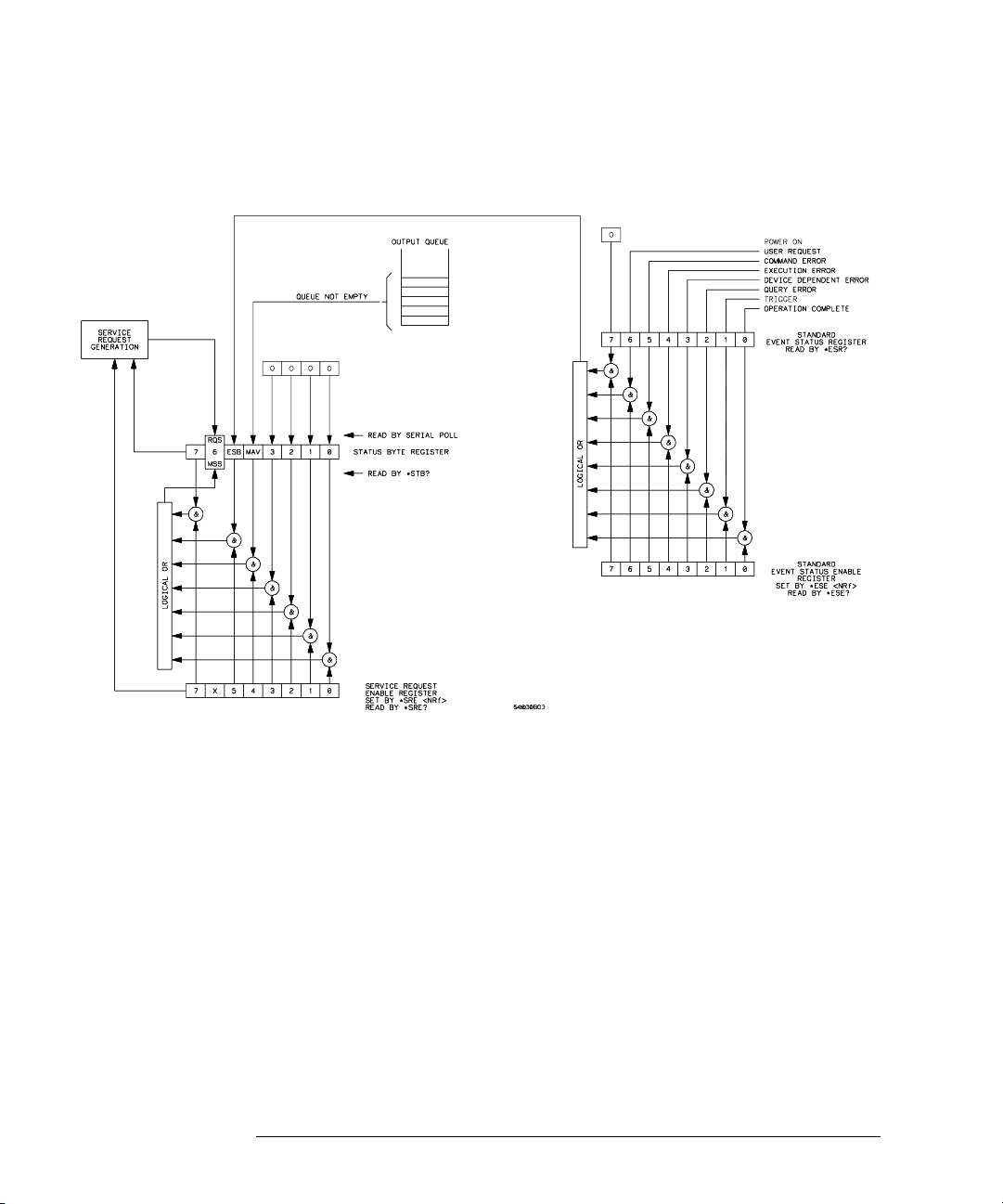
Figure 6-2

Status Reporting

Status Reporting Data Structures

6-6

Figure 6-2 (continued)

$UP

5HJ

6WDQGDUG(YHQW

6WDWXV(QDEOH 5 HJL VWHU

23(5

Status Reporting

Status Reporting Data Structures

2SHUDWLRQ 6WDWXV 5HJLVWHU

2SHUDWLRQ 6WDWXV(QDEOH 5HJLVWHU

$(5"

5XQELWV HWLI  VFRSHQRWVWRSS HG

:DLW 7ULJ

5XQ

23(5"

      

23(( 23(("



321

854

(;( ''( 4<( 54/ 23&&0(

(65"

6WDQGDUG(YHQW 6WDWXV5HJL VWHU



(6( (6("



Status Reporting Data Structures

546 06*

2XWSXW 4XHXH

75*

7(5"

5HJ

67%"

75*0$9(6%



65( 65("

7 UL JJHU (Y HQW 5HJLVWHU

6WDWXV%\WH 5HJLVWHU

6WDWXV%\WH (QDEOH5HJLVWHU



VWDWXVFGU

6-7

Status Reporting

Status Byte Register (SBR)

The Status Byte Register is the summary-level register in the status reporting structure. It contains summary bits that monitor activity in the other status registers and queues. The Status Byte Register is a live register. That is, its summary bits are set and cleared by the presence and absence of a summary bit from other event registers or queues.

If the Status Byte Register is to be used with the Service Request Enable Register to set bit 6 (RQS/MSS) and to generate an SRQ, at least one of the summary bits must be enabled, then set. Also, event bits in all other status registers must be specifically enabled to generate the summary bit that sets the associated summary bit in the Status Byte Register.

The Status Byte Register can be read using either the *STB? Common Command or the GPIB serial poll command. Both commands return the decimal-weighted sum of all set bits in the register. The difference between the two methods is that the serial poll command reads bit 6 as the Request Service (RQS) bit and clears the bit which clears the SRQ interrupt. The *STB? command reads bit 6 as the Master Summary Status (MSS) and does not clear the bit or have any affect on the SRQ interrupt. The value returned is the total bit weights of all of the bits that are set at the present time.

The use of bit 6 can be confusing. This bit was defined to cover all possible computer interfaces, including a computer that could not do a serial poll. The important point to remember is that, if you are using an SRQ interrupt to an external computer, the serial poll command clears bit 6. Clearing bit 6 allows the oscilloscope to generate another SRQ interrupt when another enabled event occurs.

No other bits in the Status Byte Register are cleared by either the *STB? query or the serial poll, except the Message Available bit (bit 4). If there are no other messages in the Output Queue, bit 4 (MAV) can be cleared as a result of reading the response to the *STB? command.

If bit 4 (weight = 16) and bit 5 (weight = 32) are set, the program prints the sum of the two weights. Since these bits were not enabled to generate an SRQ, bit 6 (weight = 64) is not set.

6-8

Status Reporting

Status Byte Register (SBR)

Example The following example uses the *STB? query to read the contents of the

oscilloscopes Status Byte Register.

10 OUTPUT 707;"*STB?" !Query the Status Byte Register 20 ENTER 707;Result !Place result in a numeric variable 30 PRINT Result !Print the result 40 End

The next program prints 112 and clears bit 6 (RQS ) of the Status Byte R egister. The difference in the decimal value between this example and the previous one is the value of bit 6 (weight = 64). Bit 6 is set when the first enabled summary bit is set and is cleared when the Status Byte Register is read by the serial poll command.

Example The following example uses the HP BASIC serial poll (SPOLL) command (GPIB

only) to read the contents of the oscilloscopes Status Byte Register.

10 Result = SPOLL(707) 20 PRINT Result 30 END

Use Serial Polling to Read Status Byte Register

Serial polling is the preferred method to read the contents of the Status Byte Register because it resets bit 6 and allows the next enabled event that occurs to generate a new SRQ interrupt.

6-9

Status Reporting

Service Request Enable Register (SRER)

Setting the Service Request Enable Register bits enable corresponding bits in the Status Byte Register. These enabled bits can then set RQS and MSS (bit 6) in the Status Byte Register.

Bits are set in the Service Request Enable Register using the *SRE command and the bits that are set are read with the *SRE? query.

Refer to figure 6-2.

Example The following example sets bit 4 (MAV) and bit 5 (ESB) in the Service Request

Enable Register.

OUTPUT 707;"*SRE 48"

This example uses the parameter 48 to enable the oscilloscope to generate an SRQ interrupt under the following conditions:

• When one or more bytes in the Output Queue set bit 4 (MAV).

• When an enabled event in the Standard Event Status Register generates a

summary bit that sets bit 5 (ESB).

Trigger Event Register (TRG)

This register sets the TRG bit in the status byte when a trigger event occurs. The TRG event register stays set until it is cleared by reading the register or

using the *CLS command. If your application needs to detect multiple triggers, the TRG event register must be cleared after each one.

If you are using the Service Request to interrupt a program or controller operation, you must clear the event register each time the trigger bit is set.

6-10

Status Reporting

Standard Event Status Register (SESR)

The Standard Event Status Register (SESR) monitors the following oscilloscope status events:

• PON - Power On

• URQ - User Request

• CME - Command Error

• EXE - Execution Error

• DDE - Device Dependent Error

• QYE - Query Error

• RQC - Request Control

• OPC - Operation Complete When one of these events occur, the event sets the corresponding bit in the

register. If the bits are enabled in the Standard Event Status Enable Register, the bits set in this register generate a summary bit to set bit 5 (ESB) in the Status Byte Register.

You can read the contents of the Standard Event Status Register and clear and the register cleared by sending the *ESR? query. The value returned is the total bit weights of all of the bits that are set at the present time.

Example The following example uses the *ESR query to read the contents of the Standard

Event Status Register.

10 OUTPUT 707;"*ESR?" 20 ENTER 707;Result !Place result in a numeric variable 30 PRINT Result !Print the result 40 End

If bit 4 (weight = 16) and bit 5 (weight = 32) are set, the program prints the sum of the two weights.

6-11

Status Reporting

Standard Event Status Enable Register (SESER)

To allow any of the Standard Event Status Register (SESR) bits to generate a summary bit, you must first enable that bit. Enable the bit by using the *ESE (Event Status Enable) common command to set the corresponding bit in the Standard Event Status Enable Register (SESER).

Set bits are read with the *ESE? query.

Example Suppose your application requires an interrupt whenever any type of error

occurs. The error related bits in the Standard Event Status Register are bits 2 through 5. The sum of the decimal weights of these bits is 60. Therefore, you can enable any of these bits to generate the summary bit by sending:

OUTPUT 707;"*ESE 60"

Whenever an error occurs, it sets one of these bits in the Standard Event Status Register. Because the bits are all enabled, a summary bit is generated to set bit 5 (ESB) in the Status Byte Register.

If bit 5 (ESB) in the Status Byte Register is enabled (via the *SRE command), an SRQ service request interrupt is sent to the external computer.

Function of SESR Bits

Standard Event Status Register bits that are not enabled still respond to their corresponding conditions (that is, they are set if the corresponding event occurs). However, because they are not enabled, they do not generate a summary bit to the Status Byte Register.

6-12

Status Reporting

User Event Register (UER)

This register hosts the LCL bit (bit 0) from the Local Event Register. The other 15 bits are reserved. You can read and clear this register using the UER? query. This register is enabled with the UEE command. For example, if you want to enable the LCL bit, you send a mask value of 1 with the UEE command; otherwise, send a mask value of 0.

Local Event Register (LCL)

This register sets the LCL bit in the User Event Register and the USR bit (bit

1) in the stat us byte. It indicates a r emote-to-local transi tion has occu rred. Th e LER? query is used to read and to clear this register.

Operation Status Register (OPR)

This register hosts the WAIT TRIG bit (bit 5), the LTEST bit (bit 8), the HIST bit (bit 9), the MASK bit (bit 10), and the PROG bit (bit 14).

• The WAIT TRIG bit is set by the Trigger Armed Event Register and indicates that the trigger is armed.

• The LTEST bit is set when a limit test fails or is completed and sets the corresponding FAIL or COMP bits in the Limit Test Event Register.

• The HI ST bit is set whe n the CO MP b it is se t in the His togram Eve n t R e g ister, indicating that the histogram measurement has satisfied the specified completion criteria.

• The MASK bit is set when the Mask Test either fails specified conditions or satisfies its completion criteria, setting the corresponding FAIL or COMP bits in the Mask Test Event Register.

• The PROG bit is reserved for future use.

• If any of these bits are set, the OPER bit (bit 7) of the Status Byte Register is set. The Operation Status Register is read and cleared with the OPER? query. The register output is enabled or disabled using the mask value supplied with the OPEE command.

6-13

Status Reporting

Limit Test Event Register (LTER)

Bit 0 (COMP) of the Limit Test Event Register is set when the Limit Test completes. The Limit Test completion criteria are set by the LTESt:RUN command.

Bit 1 (FAIL) of the Limit Test Event Register is set when the Limit Test fails. Failure criteria for the Limit Test are defined by the LTESt:FAIL command.

The Limit Test Event Register is read and cleared with the LTER? query. When either the COMP or FAIL bits are set, they in turn set the LTEST bit (bit

8) of the Operation Status Register. You can mask the COMP and FAIL bits, thus preventing them from setting the LTEST bit, by defining a mask using the LTEE command.

Enable Mask Value

Block COMP and FAIL 0 Enable COMP, block FAIL 1 Enable FAIL, block COMP 2 Enable COMP and FAIL 3

6-14

Status Reporting

Mask Test Event Register (MTER)

Bit 0 (COMP) of the Mask Test Event Register is set when the Mask Test completes. The Mask Test completion criteria are set by the MTESt:RUMode command.

Bit 1 (FAIL) of the Mask Test Event Register is set when the Mask Test fails. This will occur whenever any sample is recorded within any polygon defined in the mask.

The Mask Test Event Register is read and cleared with the MTER? query. When either the COMP or FAIL bits are set, they in turn set the MASK bit (bit

10) of the Operation Status Register. You can mask the COMP and FAIL bits,

thus preventing them from setting the MASK bit, by defining a mask using the MTEE command.

Enable Mask Value

Block COMP and FAIL 0 Enable COMP, block FAIL 1 Enable FAIL, block COMP 2 Enable COMP and FAIL 3

6-15

Status Reporting

Histogram Event Register (HER)

Bit 0 (COMP) of the Histogram Event Register is set when the Histogram completes. The Histogram completion criteria are set by the HISTogram:RUNTil command. The Histogram Event Register is read and cleared with the HER? query.

When the COMP bit is set, it in turn sets the HIST bit (bit 9) of the Operation Status Register. Results from the Histogram Register can be masked by using the HEEN command to set the Histogram Event Enable Register to the value

0. You enable the COMP bit by setting the mask value to 1.

Arm Event Register (ARM)

This register sets bit 5 (Wait Trig bit) in the Operation Status Register and the OPER bit (bit 7) in the Status Byte Register when the instrument becomes armed.

The ARM event register stays set until it is cleared by reading the register with the AER? query or using the *CLS command. If your application needs to detect multiple triggers, the ARM event register must be cleared after each one.

If you are using the Service Request to interrupt a program or controller operation when the trigger bit is set, then you must clear the event register after each time it has been set.

6-16

Status Reporting

Error Queue

As errors are detected, they are placed in an error queue. This queue is first in, first out. If the error queue overflows, the last error in the queue is replaced with error 350, Queue overflow. Any time the queue overflows, the least recent errors remain in the queue, and the most recent error is discarded. The length of the oscilloscope’s error queue is 30 (29 positions for the error messages, and 1 position for the Queue overflow message).

The error queue is read with the SYSTEM:ERROR? query. Executing this query reads and removes the oldest error from the head of the queue, which opens a position at the tail of the queue for a new error. When all the errors have been read from the queue, subsequent error queries return 0, No error.

The error queue is cleared when:

• the instrument is powered up,

• the instrument receives the *CLS common command, or

• the last item is read from the error queue.

6-17

Status Reporting

Output Queue

The output queue stores the oscilloscope-to-controller responses that are generated by certain instrument commands and queries. The output queue generates the Message Available summary bit when the output queue contains one or more bytes. This summary bit sets the MAV bit (bit 4) in the Status Byte Register.

The output queue may be read with the HP Basic ENTER statement.

Message Queue

The message queue contains the text of the last message written to the advisory line on the screen of the oscilloscope. The length of the oscilloscope’s message queue is 1. The queue is read with the SYSTEM:DSP? query. Note that messages sent with the SYSTem:DSP command do not set the MSG status bit in the Status Byte Register.

Key Queue

The key queue contains the key codes for the last 10 keys pressed on the front panel. This queue is first in, first out. If the key queue overflows, the oldest key codes are discarded as additional keys are pressed. The key queue is read with the SYSTEM:KEY? query.

Clearing Registers and Queues

The *CLS common command clears all event registers and all queues except the output queue. If *CLS is sent immediately following a program message terminator, the output queue is also cleared.

6-18

Figure 6-3

Status Reporting

Clearing Registers and Queues

Status Reporting Decision Chart

6-19

6-20

Installing and Using the Programmer’s Reference

The Programmer’s Reference is supplied as an online help file readable with the Microsoft Windows help viewer. Sample programs for the oscilloscopes are included in the Examples subdirectory.

This chapter explains how to install the help file on your system, discusses the text and program files, and explains how you can get the programs and help file via the Internet.

7-2

Installing and Using the Programmer’s Reference

To install the help file under Microsoft Windows

The help file requires Microsoft Windows 95/98/NT or greater running on an IBM-compatible PC. The file uses the Microsoft Windows help viewer, WINHELP.EXE.

1 Insert the 3.5" floppy disk labeled “Programmer’s Reference” into the

floppy disk drive of your PC.

2 Select

following:

<drive>:\setup.exe

where <drive> is your floppy disk drive letter.

3 Follow the instructions onscreen to complete the installation.

The installer copies the help file to a directory named c:\Program Files\Agilent 5462x Programmers Reference.

You can choose a different directory if desired. It also creates a Program Manager group and icon that you can use to open the help file with the Microsoft Windows help viewer.

Start | Run from the Program Manager, then type in the

7-3

Installing and Using the Programmer’s Reference

To get updated help and program files via the Internet

The latest versions of the help and example program files are available via the internet.

1 Log on to your Internet service. 2 Connect to www.agilent.com/find/5462xsw. 3 Under the “Other Software” heading in the web page, click on the

“5462x-Series Oscilloscope Programming Reference Help File,” then follow the instructions on the web page to download the help file.

7-4

Installing and Using the Programmer’s Reference

To start the help file

To open the help file under Microsoft Windows, double-click the Programmer’s Reference icon in the Programmer’s Reference program group in the Program Manager.

The help file requires the program WINHELP.EXE for Microsoft Windows 95/98/NT. The properties for the Program Manager icon are set to expect this file in the Windows directory.

To navigate through the help file

• Navigate through the help file by clicking on highlighted text and buttons.

See your Microsoft Windows documentation for more information.

7-5

7-6

Programmer’s Quick Reference

Introduction

Th e P ro gr amm er ’s Qu ic k R ef ere n ce prov ide s t h e c o mm an ds an d q u eri es with their corresponding arguments and returned formats for the oscilloscopes. The arguments for each command list the minimum argument required. The part of the command or query listed in uppercase letters refers to the short form of that command or query. The long form is the combination of the uppercase and lowercase letters. Any optional parameters are listed at the end of each parameter listing.

8-2

Programmer’s Quick Reference

Conventions

The following conventions used in this guide include:

Conventions

< > Indicates that words or characters enclosed in angular brackets

::= "is defined as." <A>::= indicates that <A> can be replaced by in any

| "or" Indicates a choice of one element from a list. For example, <A> |

... Indicates that the element preceding the ellipses may be repeated

[ ] Indicates that the bracketed items are optional. { } Indicates that when items are enclosed by braces, one, and only

{N,..,P} Indicates selection of one integer between N and P inclusive.

symbolize a program code parameter or an HP-IB command.

statement containing <A>.

indicates <A> or but not both.

one or more times.

one of the elements may be selected.

Suffix Multipliers

The following suffix multipliers are available for arguments.

EX::= 1E18 M::= 1E-3 PE::= 1E15 U::= 1E-6 T::= 1E12 N::= 1E-9 G::= 1E9 P::= 1E-12 MA::= 1E6 F::= 1E-15 K::= 1E3 A::= 1E-18

For more information regarding specific commands or queries, please refer to the online Programmer’s Reference.

8-3

Programmer’s Quick Reference

Commands and Queries

The following tables facilitate easy access to each command and query for the oscilloscopes. The commands and queries are divided into separate categories with each entry alphabetized.

The arguments for each command list the minimum argument required. The part of the command or query listed in uppercase letters refers to the short form of that command or query. The long form is the combination of the uppercase and lowercase letters. The NR1 and NR3 formats refer only to the Query Return values. Input arguments are not restricted by these formats.

These commands also show specific information about how the command operates on a particular oscilloscope model. For additional information, refer to the online oscilloscopes Programmer’s Reference.

Command Query Options and Query Returns

:ACQuire:COMPlete <complete> :ACQuire:COMPlete? <complete> ::= 100; an integer in NR1 format :ACQuire:COUNt <count> :ACQuire:COUNT? <count> ::= an integer from 1 to 16384 in NR1 format :ACQuire:MODE <mode> :ACQuire:MODE? <mode> ::= {RTIMe | ETIMe} n/a :ACQuire:POINts? 2,000; an integer in NR1 format. :ACQuire:TYPE <type> :ACQuire:TYPE? <type> ::= {NORMal | AVERage | PEAK} :ACTivity :ACTivity? <return value> ::= <edges>, <levels>

n/a :AER? {0 | 1}; an integer in NR1 format :AUToscale n/a n/a :BLANk <source> n/a <source> ::= {CHANnel<n> | POD{1 | 2} | FUNCtion} for 5462xA

n/a :CALibrate:DATE? <return value> ::= <day>,<month>,<year>; all in NR1 format :CALibrate:LABel <string> :CALibrate:LABel? <string> ::= quoted ASCII string up to 32 characters

n/a :CALibrate:SWITch? {PROTected | UNPRotected} n/a :CALibrate:TIME? <return value> ::= <hours>,<minutes>,<seconds>; all in NR1

:CDISplay n/a n/a :CHANnel<n>:BWLimit

{{0 | OFF} | {1 | ON}} :CHANnel<n>:COUPling <coupling> :C HANnel<n>:COUPling? <coupling> ::= {AC | DC | GND}; <n> ::= 1-2 or 1-4; an integer in NR1

:CHANnel<n>:DISPlay {{0 | OFF} | {1 | ON}}

:CHANnel<n>:IMPedence <impedence>

:CHANnel<n>:BWLimit? {0 | 1}; <n> ::= 1-2 or 1-4; an integer in NR1 format

:CHANnel<n>:DISPlay? {0 | 1}; <n> ::= 1-2 or 1-4; an integer in NR1 format

:CHANnel<n>:IMPedence? <impedence> ::= {ONEMeg}; <n> ::= 1-2 or 1-4; an integer in NR1

<edges> ::= presence of edges (32-bit integer in NR1 format) <levels> ::= logical highs or lows (32-bit integer in NR1 format)

<source> ::= {CHANnel<n> | DIGital0,...,DIGital15 | POD{1 | 2} | FUNCtion} for 5462xD

<n> ::= 1-2 or 1-4; an integer in NR1 format

format

8-4

Programmer’s Quick Reference

Commands and Queries

Command Query Options and Query Returns

:CHANnel<n>:INVert {{0 | OFF} | {1 | ON}}

:CHANnel<n>:LABel <string> :CHANnel<n>:LABel? <string>::= any series of 6 or less ASCII characters enclosed in

:CHANnel<n>:OFFSet <offset> [suffix]

:CHANnel<n>:PROBe <attenuation> :CHANnel<n>:PROBe? <attenuation> ::= Probe attenuation ratio in NR3 format

:CHANnel<n>:RANGe <range> [suffix]

:CHANnel<n>:SCALe <scale> [suffix] :CHANnel<n>:SCALe? <scale> ::= Vertical units per division value in NR3 format.

*CLS n/a n/a :DIGital<n>:DISPlay {{0 | OFF} | {1 |

ON}} :DIGital<n>:LABel <string> :DIGital<n>:LABel? <string>::= any series of 6 or less ASCII characters enclosed in

:DIGital<n>:POSition <position> :DIGital<n>:POSition? <n> ::= 0-15; an integer in NR1 format

:DIGital<n>:THReshold <value>[suffix]

:DIGitize [<source>[,...,<source>]] n/a <source> ::= {CHANnel<n> | POD1 | POD2 | FUNCtion} for 5462xA

:DISPlay:CLEar n/a n/a :DISPlay:DATA [format][,][area]

:DISPlay:LABel {{0 | OFF} | {1 | ON}} :DISPlay:LABel? {0 | 1} :DISPlay:LABList #80000524 <binary

block> :DISPlay:PERSistence <value> :DISPlay:PERSistence? <value> ::= {MINimum | INFinite}} :DISPlay:SOURce <value> :DISPlay:SOURce? <value> ::= {PMEMory{0 | 1 | 2}} :DISPlay:VECTors {{1 | ON} | {0 | OFF}} :DISPlay:VECTors? {1 | 0}

:CHANnel<n>:INVert? {0 | 1}; <n> ::= 1-2 or 1-4; an integer in NR1 format

quotation marks <n> ::= 1-2 or 1-4; an integer in NR1 format

:CHANnel<n>:OFFSet? <offset> ::= Vertical offset value in NR3 format.

:CHANnel<n>:RANGe? <range> ::= Vertical full-scale range value in NR3 format.

:DIGital<n>:DISPlay? {0 | 1}; <n> ::= 0-15; an integer in NR1 format

:DIGital<n>:THReshold? <n> ::= 0-15; an integer in NR1 format

:DISPlay:DATA? [format][,][area] <format> ::= {TIFF} (command only)

:DISPlay:LABList? <binary block> ::= a time-ordered list of 75 labels. Each label can

[suffix] ::= {V} <n> ::= 1-2 or 1-4; an integer in NR1 format

::= X1, X10, X20, X100 (obsolete form) <n> ::= 1-2 or 1-4; an integer in NR1 format

[suffix] ::= {V} <n> ::= 1-2 or 1-4; an integer in NR1 format

quotation marks <n> ::= 0-15; an integer in NR1 format

<position> ::= 1-8 if display size = large, 1-16 if size = medium, 132 if size = small

<value> ::= {CMOS | ECL | TTL | <user defined value>} <user defined value> ::= value in NR3 format from -8.00 to +8.00 [suffix] ::= {V | mV (-3) | mV (-6)}

<source> ::= {CHANnel<n> | DIGital0,...,DIGital15 | POD1 | POD2 | FUNCtion} for 5462xD

<source> can be repeated up to 5 times. <n> ::= 1-2 or 1-4; an integer in NR1 format

<area> ::= {GRATicule} (command only) <format> ::= {TIFF | BMP} (query only) <area> ::= {GRATicule | SCReen} (query only) <binary block_data> ::= data in IEEE 488.2 # format

be a maximum of 6 characters followed by a comma.

8-5

Programmer’s Quick Reference

Commands and Queries

Command Query Options and Query Returns

*DMC <macro label>,<macro definition>

*EMC {{0 | OFF} | {1 | ON}} *EMC? {0 | 1} *ESE <mask> *ESE? <mask> ::= 0 to 255; an integer in NR1 format

n/a *ESR? <status> ::= 0 to 255; an integer in NR1 format :FUNCtion:CENTer <frequency> :FUNCtion:CENTer? <frequency> ::= the current center frequency in NR3 format.

:FUNCtion: DISPlay {{0 | OFF} | {1 | ON}} :FUNCtion:DISPlay? {0 | 1} :FUNCtion:OFFSet <offset> :FUNCtion:OFFSet? <offset> ::= the value at center screen in NR3 format.

:FUNCtion:OPERation <operation> :FUNCtion:OPERat ion? < operation> ::= {SUBTra ct | MULTiply | INTegrate | DIF Ferentiat e

:FUNCtion:RANGe <range> :FUNCtion:RANGe? <range> ::= the full-scale vertical axis value in NR3 format.

:FUNCtion:REFerence <level> :FUNCtion:REFerence? <level> ::= the current reference level in NR3 format.

:FUNCtion:SCALe <scale value>[<suffix>]

:FUNCtion:SOURce <source> :FUNCtion:SOURce? <source> ::= {CHANnel<n> | ADD | SUBT | MULT}; <n> ::= 1-2 or

:FUNCtion:SPAN :FUNCtion:SPAN? ::= the current frequency span in NR3 format.

:FUNCtion:WINDow <window> :FUNCtion:WINDow? <window> ::= {RECTangular | HANNing | FLATtop} n/a *GMC? <macro label> <macro label> ::= quoted ASCII string, block data in IEEE 488.2 #

:HARDcopy:DESTination <destination>

:HARDcopy:FACTors {{0 | OFF} | {1 | ON}}

:HARDcopy:FFEed {{0 | OFF} | {1 | ON}} :HARDcopy:FFEed? {0 | 1} :HARDcopy:FORMat <device> :HARDcopy:FORMat? <format> ::= {TIFF | BMP | CSV | LASerjet | DESKjet | EPSon |

n/a <macro label> ::= quoted ASCII string

:FUNCtion:SCALe <scale value> ::= integer in NR1 format

:HARDcopy:DESTination <destination> ::= {CENTronics | FLOPpy}

:HARDcopy:FACTors? {0 | 1}

<macro definition> ::= block data in IEEE 488.2 # format

Bit Weight Enables 7 128 PON - Power On 6 64 URQ - User Request 5 32 CME - Command Error 4 16 EXE - Execution Error 3 8 DDE - Device Dependent Error 2 4 QYE - Query Error 1 2 TRG - Trigger Query 0 1 OPC - Operation Complete

The range of legal values is from 0 Hz to 25.00 GHz.

The range of legal values is +/-10 times the current sensitivity of the selected function.

| FFT}

The range for ADD, SUBT, MULT is 8E-6 to 800E+3. The range for the INTegrate function is 8E-9 to 400E+3. The range for the DIFFerentiate function is 80E-3 to 8.0E12

(depends on current sweep speed). The range for the FFT function is 8 to 800 dBV.

The range of legal values is from 400.0 dBV to +400.0 dBV (depending on current range value).

<suffix> ::= {V | dB}

1-4 in NR1 format

Legal values are 1 Hz to 100 GHz

format

SEIKo}

8-6

Programmer’s Quick Reference

Commands and Queries

Command Query Options and Query Returns

:HARDcopy:GRAYscale {{0 | OFF} | {1 | ON}}

n/a *IDN? AGILENT TECHNOLOGIES,<model>, <serial number>,X.XX.XX

n/a *LMC? <ascii string> ::= string list seperated by commas n/a *LRN? <learn_string> ::= current instrument setup as a block of data in

:MEASure:CLEar n/a n/a :MEASure:DUTYcycle [<source>] :MEASure:DUTYcycle?

:MEASure:FALLtime [<source>] :MEASure:FALLtime? [<source>] <source> ::= {CHANnel<n> | FUNCtion | MATH} for 5462xA

:MEASure:FREQuency [<source>] :MEASure:FREQuency?

:MEASure:NWIDth [<source>] :MEASure:NWIDth? [<source>] <source> ::= {CHANnel<n> | FUNCtion | MATH} for 5462xA

:MEASure:OVERshoot [<source>] :MEASure:OVERshoot?

:MEASure:PERiod [<source>] :MEASure:PERiod? [<source>] <source> ::= {CHANnel<n> | FUNCtion | MATH} for 5462xA

:MEASure:PREShoot [<source>] :MEASure:PREShoot? [<source>] <source> ::= {CHANnel<n> | FUNCtion | MATH}

:MEASure:PWIDth [<source>] :MEASure:PWIDth? [<source>] <source> ::= {CHANnel<n> | FUNCtion | MATH} for 5462xA

:HARDcopy:GRAYscale? {0 | 1}

<model> ::= the model number of the instrument <serial number> ::= the serial number of the instrument <X.XX.XX> ::= the software revision of the instrument

IEEE 488.2 # format

[<source>]

<source> ::= {CHANnel<n> | FUNCtion | MATH} for 5462xA <source> ::= {CHANnel<n> | DIGital0,...,DIGital15 | FUNCtion |

MATH} for 5462xD <n> ::= 1-2 or 1-4 in NR1 format <return_value> ::= ratio of positive pulse width to period in NR3

format

<source> ::= {CHANnel<n> | DIGital0,...,DIGital15 | FUNCtion | MATH} for 5462xD

<n> ::= 1-2 or 1-4 in NR1 format <return_value> ::= time in seconds between the lower and upper

thresholds in NR3 format <source> ::= {CHANnel<n> | FUNCtion | MATH}

<n> ::= 1-2 or 1-4 in NR1 format <return_value> ::= frequency in Hertz in NR3 format

<source> ::= {CHANnel<n> | DIGital0,...,DIGital15 | FUNCtion | MATH} for 5462xD

<n> ::= 1-2 or 1-4 in NR1 format <return_value> ::= negative pulse width in seconds-NR3 format

<source> ::= {CHANnel<n> | FUNCtion | MATH} <n> ::= 1-2 or 1-4 in NR1 format <return_value> ::= the percent of the overshoot of the selected

waveform in NR3 format

<source> ::= {CHANnel<n> | DIGital0,...,DIGital15 | FUNCtion | MATH} for 5462xD

<n> ::= 1-2 or 1-4 in NR1 format <return_value> ::= waveform period in seconds in NR3 format

<n> ::= 1-2 or 1-4 in NR1 format <return_value> ::= the percent of preshoot of the selected

waveform in NR3 format

<source> ::= {CHANnel<n> | DIGital0,...,DIGital15 | FUNCtion | MATH} for 5462xD

<n> ::= 1-2 or 1-4 in NR1 format <return_value> ::= width of positive pulse in seconds in NR3

format

8-7

Programmer’s Quick Reference

Commands and Queries

Command Query Options and Query Returns

:MEASure:RISEtime [<source>] :MEASure: RISEtime? [<source>] <source> ::= {CHANnel<n> | FUNCtion | MATH}

:MEASure:SHOW {1 | ON} :MEASure:SHOW? {1} :MEASure:SOURce [<source>] :MEASure:SOURce? <source> ::= {CHANnel<n> | FUNCtion | MATH} for 5462xA

:MEASure:TEDGe <slope><occurrence>[,<source>]

:MEASure:TMAX [<source>] :MEASure:TMAX? <source> ::= {CHANnel<n> | FUNCtion | MATH} for 5462xA

n/a :MEASure:TVALue? <value>,

:MEASure:VAMPlitude [<source>] :MEASure:VAMPlitude?

:MEASure:VAVerage [<source>] :MEASure:VAVerage? [<source>] <source> ::= {CHANnel<n> | FUNCtion | MATH}

:MEASure:VBASe [<source>] :MEASure:VBASe? [<source>] <source> ::= {CHANnel<n> | FUNCtion | MATH}

:MEASure:VMAX [<source>] :MEASure:VMAX? [<source>] <source> ::= {CHANnel<n> | FUNCtion | MATH}

:MEASure:VMIN [<source>] :MEASure:VMIN? [<source>] <source> ::= {CHANnel<n> | FUNCtion | MATH}

:MEASure:TEDGe? <slope> ::= direction of the waveform

[<slope>]<occurrence>[,<source >]

[<source>]

<n> ::= 1-2 or 1-4 in NR1 format <return_value> ::= rise time in seconds in NR3 format

<source> ::= {CHANnel<n> | DIGital0,...,DIGital15 | FUNCtion | MATH} for 5462xD

<n> ::= 1-2 or 1-4 in NR1 format for HP5462xA <return_value> ::= {<source> | <none>} <none> ::= query returns “NONE” if all channels are off

<occurrence> ::= the transition to be reported. <source> ::= {CHANnel<n> | FUNCtion | MATH} for 5462xA <source> ::= {CHANnel<n> | DIGital0,...,DIGital15 | FUNCtion |

MATH} for 5462xD <n> ::= 1-2 or 1-4 in NR1 format for HP5462xA <return_value> ::= time in seconds of the specified transition

<source> ::= {CHANnel<n> | DIGital0,...,DIGital15 | FUNCtion | MATH} for 5462xD

<n> ::= 1-2 or 1-4 in NR1 format for HP5462xA <value> ::= voltage level that the waveform must cross.

<slope> ::= direction of the waveform when <value> is crossed. <occurrence> ::= transitions reported. <return_value> ::= time in seconds of specified voltage crossing

in NR3 format <source> ::= {CHANnel<n> | FUNCtion | MATH} for 5462xA <source> ::= {CHANnel<n> | DIGital0,...,DIGital15 | FUNCtion |

MATH} for 5462xD <n> ::= 1-2 or 1-4 in NR1 format

<source> ::= {CHANnel<n> | FUNCtion | MATH} <n> ::= 1-2 or 1-4 in NR1 format <return_value> ::= the amplitude of the selected waveform in

volts in NR3 format

<n> ::= 1-2 or 1-4 in NR1 format <return_value> ::= calculated average voltage in NR3 format

<n> ::= 1-2 or 1-4 in NR1 format <base_voltage> ::= voltage at the base of the selected waveform

in NR3 format

<n> ::= 1-2 or 1-4 in NR1 format <ret urn_value > ::= max imum vol tage of th e selec ted wavef orm in

NR3 format

<n> ::= 1-2 or 1-4 in NR1 format <return_value> ::= minimum voltage of the selected waveform in

NR3 format

8-8

Agilent 54621D Programmer’s Guide

Specifications and Main Features

Frequently Asked Questions

User Manual

Programming the Oscilloscope

In This Book

Contents

Introduction to Programming

Talking to the Instrument

Program Message Syntax

Combining Commands from the Same Subsystem

Duplicate Mnemonics

Query Command

Program Header Options

Program Data Syntax Rules

Program Message Terminator

Selecting Multiple Subsystems

Programming Getting Started

Initialization

Autoscale

Setting Up the Instrument

Example Program

Using the DIGitize Command

Receiving Information from the Instrument

String Variables

Numeric Variables

Definite-Length Block Response Data

Multiple Queries

Instrument Status

Programming over GPIB

Interface Capabilities

Command and Data Concepts

Addressing

Communicating Over the Bus

Lockout

Bus Commands

Programming over RS-232-C

Interface Operation

Cables

Minimum Three-Wire Interface with Software Protocol

Extended Interface with Hardware Handshake

Configuring the Interface

Interface Capabilities

Communicating Over the RS-232-C Bus

Programming and Documentation Conventions

Command Set Organization

The Command Tree

Obsolete and Discontinued Commands

Truncation Rules

Infinity Representation

Sequential and Overlapped Commands

Response Generation

Notation Conventions and Definitions

Program Examples

Status Reporting

Status Reporting Data Structures

Status Byte Register (SBR)

Service Request Enable Register (SRER)

Trigger Event Register (TRG)

Standard Event Status Register (SESR)

Standard Event Status Enable Register (SESER)

User Event Register (UER)

Local Event Register (LCL)

Operation Status Register (OPR)

Limit Test Event Register (LTER)

Mask Test Event Register (MTER)

Histogram Event Register (HER)

Arm Event Register (ARM)

Error Queue

Output Queue

Message Queue

Key Queue

Clearing Registers and Queues

Installing and Using the Programmer’s Reference

To install the help file under Microsoft Windows

To get updated help and program files via the Internet

To start the help file

To navigate through the help file

Programmer’s Quick Reference

Conventions