Agilent 0B Series Programming Datasheet

Download

Page 1

Agilent 86140B Series Optical Spectrum Analyzer

Programming Guide

Agilent Technologies

Page 2

Notices

This document contains proprietary information that is protected by copyright. All rights are reserved.

No part of this document may reproduced in (including electronic storage and retrieval or translation into a foreign language) without prior agreement and written consent from Agilent Technologies GmbH as governed by United States and international copyright laws.

Agilent Technologies Deutschland GmbH Herrenberger Str. 130 71034 Böblingen Germany

Manual Part Number

86140-90069

Edition

Second edition, January 2005

First edition, January 2002

Warranty

This Agilent Technologies instrument product is warranted against defects in material and workmanship for a period of one year from date of shipment. During the warranty period, Agilent will, at its option, either repair or replace products that prove to be defective. For warranty service or repair, this product must be returned to a service facility designated by Agilent. Buyer shall prepay shipping charges to Agilent and Agilent shall pay shipping charges to return the product to Buyer. However, Buyer shall pay all shipping charges, duties, and taxes for products returned to Agilent from another country.

Agilent warrants that its software and firmware designated by Agilent for use with an instrument will execute its programming instructions when

properly installed on that instrument. Agilent does not warrant that the operation of the instrument, software, or firmware will be uninterrupted or error free.

Limitation of Warranty

The foregoing warranty shall not apply to defects resulting from improper or inadequate maintenance by Buyer, Buyer-supplied software or interfacing, unauthorized modification or misuse, operation outside of the environmental specifications for the product, or improper site preparation or maintenance. No other warranty is expressed or implied. Agilent Technologies specifically disclaims the implied warranties of Merchantability and Fitness for a Particular Purpose.

Exclusive Remedies

The remedies provided herein are Buyer's sole and exclusive remedies. Agilent Technologies shall not be liable for any direct, indirect, special, incidental, or consequential damages whether based on contract, tort, or any other legal theory.

Assistance

Product maintenance agreements and other customer assistance agreements are available for Agilent Technologies products. For any assistance contact your nearest Agilent Technologies Sales and Service Office.

Certification

Agilent Technologies Inc. certifies that this product met its published specifications at the time of shipment from the factory. Agilent Technologies further certifies that its calibration measurements are traceable to the United States National Institute of Standards and Technology, NIST (formerly the United States

National Bureau of Standards, NBS) to the extent allowed by the Institutes’s

calibration facility, and to the calibration facilities of other International Standards Organization members.

ISO 9001 Certification

Produced to ISO 9001 international quality system standard as part of our objective of continually increasing customer satisfaction through improved process control.

Safety Notices

CAUTION

A CAUTION notice denotes a hazard. It calls attention to an operating procedure, practice, or the like that, if not correctly per formed or adhered to, could result in damage to the product or loss of important data. Do not proceed beyond a CAUTION notice until the indicated conditions are fully understood and met.

WARNING

A WARNING notice denotes a hazard. It calls attention to an operating procedure, practice, or the like that, if not correctly performed or adhered to, could result in personal injury or death. Do not proceed beyond a WARNING notice until the indi cated conditions are fully understood and met.

Page 3

Warnings and Notices

WARNING

To avoid the possibility of injury or death, you must observe the fol lowing precautions before switching on the instrument. Insert the power cable plug only into a socket outlet provided with a protective earth contact. Do not negate this protective action by the using an extension cord without a protective conductor.

WARNING

Never look directly into the end of a fiber or a connector, unless you are absolutely certain that there is no signal in the fiber.

Page 4

Agilent Technologies Sales and Service Offices

For more information about Agilent Technologies test and measurement products, applications, services, and for a current sales office listing, viesit our web site:

http://www.agilent.com/comms/lightwave

You can also contact one of the following centers and ask for a test and measurement sales representative.

United States: 1 800 452 4844

1 888 900 8921 (FAX)

Canada: 1 877 894 4414

(905) 282 6495 (FAX)

Europe: (31 20) 547 2111

(43 20) 547 2190 (FAX)

Japan: 0120 421 345

0120 421 678 (FAX)

Mexico (52 55) 5081 9469

(52 55) 5081 9467 (FAX)

Australia: 1 800 629 485

1 800 142 134 (FAX)

Asia-Pacific: (852) 3197 7889

(852) 2506 9233 (FAX)

Brazil (55 11) 4197 3600

(55 11) 4197 3800 (FAX)

Page 5

Remote Operation 7

General Safety Considerations 8

Safety Symbols 8

Summary for Experienced GPIB Programmers 11 Working with Older OSA Applications 16 Introduction to Controlling an OSA 18 SCPI Syntax Rules 23 Monitoring the Instrument 29 Amplitude Correction Remote Commands 32 Techniques to Improve Throughput 34 Sending Remote Commands over the LAN 39

SICL LAN Set-up Information 40 Setting Up Your Analyzer as a SICL LAN Server 40 Setting Up Your Controller as a SICL LAN Client 41

Example Programs 43

Example 1. Initialization and a simple measurement 44 Example 2. Locating the largest signal 46 Example 3. Bandwidth 47 Example 4. Maximum and minimum amplitude values 49 Example 5. Maximum and minimum values over time 51 Example 6. Returning trace data 52 Example 7. Trace normalization 54 Example 8. Total power measurement 55 Example 9. Monitoring the status registers 56 Example 10 SMSR calculation with display off 58

Front Panel Functions to Remote Commands 60

Programming Commands 67

Introduction 68 Command Conventions 69 Command Trees 71

Agilent 86140B Optical Spectrum Analyzer, Second Edition 5

Page 6

Common Commands 79 CALCulate Subsystem Commands 89 CALibration Subsystem Commands 156 DISPlay Subsystem Commands 172 FORMat Subsystem Commands 184 HCOPy Subsystem Commands 185 INITiate Subsystem Commands 189 INPut Subsystem Commands 191 INSTrument Subsystem Commands 200 MEMory Subsystem Commands 203 MMEMory Subsystem Commands 204 ROUTe Subsystem Commands 208 SENSe Subsystem Commands 209 SOURce[n] Subsystem Commands 230 STATus Subsystem Commands 233 SYSTem Subsystem Commands 238 TRACe Subsystem Commands 247 TRIGger Subsystem Commands 254 UNIT Subsystem Commands 258 Agilent 71450 Series Commands to Agilent 86140B

Series Equivalents

Agilent 71450 series commands available on the Agilent 86140B series 273

260

Index 275

6 Agilent 86140B Optical Spectrum Analyzer, Second Edition

Page 7

Remote Operation

General Safety Considerations. . . . . . . . . . . . . . . . . . . . . . . .8

Safety Symbols . . . . . . . . . . . . . . . . . . . . . . . . . . . . . . . . . . . . . . . . . 8

Summary for Experienced GPIB Programmers . . . . . . . . . 11

Working with Older OSA Applications . . . . . . . . . . . . . . . .16

Introduction to Controlling an OSA . . . . . . . . . . . . . . . . . . .18

SCPI Syntax Rules . . . . . . . . . . . . . . . . . . . . . . . . . . . . . . . . .23

Monitoring the Instrument . . . . . . . . . . . . . . . . . . . . . . . . . .29

Techniques to Improve Throughput. . . . . . . . . . . . . . . . . . .34

Sending Remote Commands over the LAN . . . . . . . . . . . .39

SICL LAN Set-up Information . . . . . . . . . . . . . . . . . . . . . . . . . . . .40

Setting Up Your Analyzer as a SICL LAN Server . . . . . . . . . . . . 40

Setting Up Your Controller as a SICL LAN Client . . . . . . . . . . . .41

Example Programs . . . . . . . . . . . . . . . . . . . . . . . . . . . . . . . . .43

Example 1. Initialization and a simple measurement . . . . . . . .44

Example 2. Locating the largest signal . . . . . . . . . . . . . . . . . . . .46

Example 3. Bandwidth . . . . . . . . . . . . . . . . . . . . . . . . . . . . . . . . . .47

Example 4. Maximum and minimum amplitude values. . . . . . .49

Example 5. Maximum and minimum values over time . . . . . . . 51

Example 6. Returning trace data. . . . . . . . . . . . . . . . . . . . . . . . . .52

Example 7. Trace normalization . . . . . . . . . . . . . . . . . . . . . . . . . .54

Example 8. Total power measurement. . . . . . . . . . . . . . . . . . . . .55

Example 9. Monitoring the status registers . . . . . . . . . . . . . . . .56

Example 10 SMSR calculation with display off . . . . . . . . . . . . .58

Front Panel Functions to Remote Commands . . . . . . . . . .60

Agilent 86140B Optical Spectrum Analyzer, Second Edition 7

Page 8

Remote Operation General Safety Considerations

General Safety Considerations

This product has been designed and tested in accordance with the standards listed on the Manufacturer’s Declaration of Conformity, and has been supplied in a safe condition. The documentation contains information and warnings that must be followed by the user to ensure safe operation and to maintain the product in a safe condition.

Install the instrument according to the enclosure protection provided. This instrument does not protect against the ingress of water. This instrument protects against finger access to hazardous parts within the enclosure.

CAUTION

WARNING

Safety Symbols

The caution sign denotes a hazard. It calls attention to a procedure which, if not correctly performed or adhered to, could result in damage to or destruction of the product. Do not proceed beyond a caution sign until the indicated conditions are fully understood and met.

The warning sign denotes a hazard. It calls attention to a procedure which, if not correctly performed or adhered to, could result in injury or loss of life. Do not proceed beyond a warning sign until the indicated conditions are fully understood and met.

8 Agilent 86140B Optical Spectrum Analyzer, Second Edition

Page 9

General Safety Considerations Remote Operation

WARNING

If this product is not used as specified, the protection provided by the equipment could be impaired. This product must be used in a normal condition (in which all means for protection are intact) only.

No operator serviceable parts inside. Refer servicing to qualified service personnel. To prevent electrical shock do not remove covers.

This is a Safety Class 1 Product (provided with a protective earthing ground incorporated in the power cord). The mains plug shall only be inserted in a socket outlet provided with a protective earth contact. Any interruption of the protective conductor inside or outside of the instrument is likely to make the instrument dangerous. Intentional interruption is prohibited.

To prevent electrical shock, disconnect the instrument from mains before cleaning. Use a dry cloth or one slightly dampened with water to clean the external case parts. Do not attempt to clean internally.

CAUTION

or damaged cables and accessories. The Agilent 86140B series’s front-panel INPUT connector is no exception. When you use improper cleaning and handling techniques, you risk expensive instrument repairs, damaged cables, and compromised measurements. Before you connect any fiber-optic cable to the Agilent 86140B series, refer to “Cleaning Connectors for Accurate Measurements” in the usesr’s guide.

This product is designed for use in Installation Category II and

Fiber-optic connectors are easily damaged when connected to dirty

CAUTION

Pollution Degree 2 per IEC 61010-1C and 664 respectively.

Do not use too much liquid in cleaning the Optical Spectrum

CAUTION

Analyzer. Water can enter the front-panel keyboard, damaging sensitive electronic components.

Agilent 86140B Optical Spectrum Analyzer, Second Edition 9

Page 10

Remote Operation General Safety Considerations

CAUTION

VENTILATION REQUIREMENTS: When installing the product in a cabinet, the convection into and out of the product must not be restricted. The ambient temperature (outside the cabinet) must be less than the maximum operating temperature of the product by 4 C for every 100 watts dissipated in the cabinet. If the total power dissipated in the cabinet is greater than 800 watts, then forced convection must be used.

Install the instrument so that the detachable power cord is readily identifiable and is easily reached by the operator. The detachable power cord is the instrument disconnecting device. It disconnects the mains circuit from the mains supply before other parts of the instrument. The front panel switch is only a standby switch and is not a LINE switch. Alternatively, an externally installed switch or circuit breaker (which is readily identifiable and is easily reached by the operator) may be used as a disconnecting device.

Always use the three-prong AC power cord supplied with this instrument. Failure to ensure adequate earth grounding by not using this cord may cause instrument damage.

CAUTION

This instrument has autoranging line voltage input. Be sure the supply voltage is within the specified range.

The Agilent 86140B, 86141B, and 86142B Option 004/005 EELED sources contain an IEC Class 1 LED, according to IEC 60825.

Use of controls or adjustment or performance of procedures other than those specified herein may result in hazardous radiation exposure.

10 Agilent 86140B Optical Spectrum Analyzer, Second Edition

Page 11

Summary for Experienced GPIB Programmers Remote Operation

Summary for Experienced GPIB Programmers

This section is intended for people who are familiar with GPIB instrument programming. Terms like EOI, command synchronization and SCPI should be familiar to you. If not, review the following sections in this chapter. This section is a summary to get your OSA application operating quickly, focusing on ways in which the OSA differs from other instruments you may have encountered.

Auto Align

The optical spectrum analyzer contains optics that can drift out of alignment with environmental variations such as air pressure, temperature and humidity. To compensate for this, the Auto Align routine should be run when the instrument has been turned on, warmed up and stabilized, and whenever the temperature changes more than 1 degree centigrade. Since temperature is difficult to monitor, the rule of thumb is to auto align every 8 hours for normal applications, and once an hour for applications that require high amplitude stability or accuracy.

To perform the Auto Align routine, connect a stable input signal and then send a CAL marker 1 on the desired signal and use the marker align command CALIBRATE:ALIGN:MARKER 1. Using the marker allows you to select the appropriate signal.

IBRATE:ALIGN command. The preferred method is to position

EOI required

Before sending remote commands to the instrument, set your GPIB interface to assert the GPIB END message (also called EOI) with the last character of the transmission. There is a separate GPIB signal line dedicated to EOI, and when the OSA sees the EOI, it closes the buffer and begins processing the commands. The OSA will not accept any more commands until it has parsed and launched (but not necessarily completed) all the commands in the buffer.

Most interfaces use EOI by default. If, for example, you are using a National Instruments GPIB card with Visual C or Visual Basic, EOI is probably on. Similarly, if you are using an Agilent GPIB card in a HP-UX workstation, programming in C or C++, EOI is probably on. If you are using Basic for Windows, you will need to enable EOI each time you open a session to the instrument. This is done using the ASSIGN @OSA key words, and associating the END keyword with the session.

Agilent 86140B Optical Spectrum Analyzer, Second Edition 11

Page 12

Remote Operation Summary for Experienced GPIB Programmers

Turn the input buffer on

To provide compatibility with earlier firmware revisions, the input buffer is disabled in the OSA default state. In order to get the faster and more regular behavior, turn the buffer on each time you preset the instrument using:

SENDCOMMAND SYST:COMM:GPIB:BUFF ON

Note that front panel preset or remote *RST will reset the OSA to default conditions and also turns the input buffer off. You may also wish to turn the buffer off by sending:

SENDCOMMAND SYST:COMM:GPIB:BUFF OFF

Use device clear

The OSA uses the Selected Device Clear interface message to free the instrument from error conditions. Clearing the instrument at the start of any control application will avoid confusing the instrument. You may find it useful to write a small program that does nothing but clear the instrument, so you can clear it when you need to as you debug your application.

Note that Selected Device Clear is not a text message like *CLS. It is an interface level command. For VISA, use

VICLEAR(). For NI 488.2, use IBCLR().

For Agilent SICL, use ICLEAR(). For Basic for windows, use CLEAR 723 or CLEAR @OSA.

Use single sweep mode

When using remote programming, you will want the instrument to take a sweep only after it is set up and you want the sweep to occur. Allowing the instrument to sweep while you are sending commands significantly slows the instrument down. In general, unless an operator is tuning a device, it is best to turn continuous sweep off with:

INITIATE:CONTINUOUS OFF

The *RST command automatically turns continuous sweep off.

Command synchronization

The OSA may start executing the next command before finishing the previous one. This is common among GPIB controlled instruments - it allows the instrument’s multi-tasking operating system to execute commands as quickly as possible. Because of this, you will need to use *OPC, *OPC? or *WAI to find out when a sweep is finished before attempting to read data from the instrument. Most commonly, you will send an INIT

IATE command to take a single sweep, then wait for the sweep

12 Agilent 86140B Optical Spectrum Analyzer, Second Edition

Page 13

Summary for Experienced GPIB Programmers Remote Operation

to finish before executing the next command. You also need to wait for any command that starts with “AUTO”, such as automeasure or autoalign, and for any commands that perform a calibration.

The recommended technique for waiting is to use the query form of *OPC (*OPC?). This way, after initiating the sweep, you can do other things while waiting for the instrument. When you do wait, make sure your GPIB timeout is longer than what the instrument needs to finish the command. A typical sequence would be:

SENDMESSAGE INIT;*OPC? // take a sweep

//perform other tasks while waiting

RECEIVEINTEGER // wait for “1” indicating end of sweep

Other alternatives involve polling the instrument for status, and that in turn slows the instrument down by making it respond to the queries. If you must poll for status, it is recommended that you send *ESE 1 to enable the OPC bit to set bit 5 of the main status register, then use serial poll to query the main status register.

Serial poll is a GPIB interface level operation, not a command like *STB?. It is accessed using special commands. For VISA, use

VIREADSTB. For NI

488.2, use IBRSP. For SICL, use IREADSTB(). For Basic for Windows, use SPOLL 723 or SPOLL @OSA.

Once the OPC bit is set, you will need to manually clear the status register. The easiest way to do this is to send *CLS. You can also clear it by reading the register with *ESR?

If you don’t need an explicit response from the instrument, the *WAI command will cause the instrument to finish processing all prior commands before continuing.

Maximum query rate

If you are waiting for a bit in a status byte, avoid writing a tight loop that continuously queries the instrument. This causes the instrument firmware to spend an excessive amount of time responding to your queries rather than running the instrument. Do not query the instrument more than once every 5 ms. For Visual Basic and Visual C, use the SLEEP command to put 5 ms delay in your query loop. For posix compliant platforms, use the

NANOSLEEP() function to delay the loop. For Basic for Windows, use WAIT

0.005.

Watching for error messages

Whenever an error occurs, it appears briefly on the instrument display and is added to the error queue. Whenever there are messages in the error queue, bit 2 of the status byte is set. The recommended practice is to use serial poll to read the status byte and then use a bitwise ‘and’ against the

Agilent 86140B Optical Spectrum Analyzer, Second Edition 13

Page 14

Remote Operation Summary for Experienced GPIB Programmers

value 4 to see if the bit is set. If it is set, you should use SYSTEM:ERROR? to read all the error messages until you get a response that begins with “+0”, indicating no further errors.

As you are developing your application, you should check the error status every time you read from or write to the instrument.

Most commonly used commands

The most commonly used commands are listed here. For commands that are listed twice, the first listing is the short form, the second is the long form. Most SCPI commands have a long form that is easier to understand but takes longer to send. The long form is listed only for your understanding and for cross referencing elsewhere in the manual. In practice, you should use the short form.

Table 1 Most commonly used GPIB commands

Command Usage

SELECTED DEVICE CLEAR This is not a text command - it is a GPIB hardware message

you should use to start off your application.

*RST The second thing you should do in your application to return

the instrument to a known state and set single sweep mode.

SYST:COMM:GPIB:BUFF ON

EM:COMM:GPIB:BUFFER ON|OFF

SYST

CENT 1550

Turn the GPIB input buffer on and allow parallel command execution.

Program the center wavelength, in nm.

[SENSE:][WAVELENGTH:]CENTER

SPAN, STAR

BAND 2

T, STOP Other wavelength oriented commands.

Set the resolution bandwidth to 2 nm.

[SENSE:]BANDWIDTH:[RESOLUTION]

POW:RANG:LOW -45

DBM

[SENSE:]POWER:[DC:]RANGE:LOWER

Tell the instrument the lowest power you expect to see, causing the instrument to adjust its sensitivity. Impacts sweep time.

POW:RANG:AUTO OFF [SENS

E:]POWER:[DC:]RANGE:AUTO ON|OFF

Turn off auto-ranging - the automatic changing of gain range during a sweep. Use POW:RANG:LOW and DISP:TRAC:Y:RLEV to select the minimum and maximum powers expected.

DISP:TRAC:Y:RLEV-10

DBM

DISPLAY:[WINDOW[1]:]TRACE:Y[1,2]:[SCALE:]RLEVEL

INIT

IATE:[IMMEDIATE]

INIT

Set the display reference level - the maximum power expected to display.

Tak e a s we ep.

*OPC? Instrument returns a “1” when all GPIB commands received

prior to the *OPC? are complete.

*WAI Instrument stops processing new GPIB commands until all

GPIB commands receiver prior to *WAI are complete.

14 Agilent 86140B Optical Spectrum Analyzer, Second Edition

Page 15

Summary for Experienced GPIB Programmers Remote Operation

Table 1 Most commonly used GPIB commands

Command Usage

CALC:MARK1:MAX CALC

ULATE:MARKER[1|2|3|4]:MAXIMUM

CALC:MARK1:X?

ULATE:MARKER[1|2|3|4]:X?

CALC

CALC:MARK1:Y?

ULATE:MARKER[1|2|3|4]:Y?

CALC

CALC:MARK1:FUNC:NOISE ON

ULATE:MARKER[1|2|3|4]:FUNCTION:NOISE:[STATE:]

CALC

Positions marker 1 to the maximum amplitude point.

Read back marker 1 wavelength.

Read back marker 1 amplitude.

Turn noise marker on for marker 1.

ON|OFF

CALC:MARK1:FUNC:NOIS:RES?

ULATE:MARKER[1|2|3|4]:FUNCTION:NOISE:RESULT?

CALC

Read back noise marker value, noise power normalized to 1 nm (or 0.1 nm if specified with noise marker bandwidth function).

TRAC? TRA

E:[DATA:][Y]? TRA|TRB|TRC|TRD|TRE|TRF

TRAC

Transfer entire trace, according to format set with the FORM command.

*IDN? Return string describing model number, serial number and

software version.

SYST:ERR? Read error at top of queue.

DISP OFF

LAY:[WINDOW[1]] ON|OFF

DISP

Turn the display off, without affecting the instrument state. Takes about 12 seconds.

Agilent 86140B Optical Spectrum Analyzer, Second Edition 15

Page 16

Remote Operation Working with Older OSA Applications

Working with Older OSA Applications

This user’s guide applies to OSA’s with firmware revision B.04.00 and later. If you have an application written for OSA’s with earlier firmware, your application will still run. The instrument defaults to a backward-compatible mode. There will be a small speed improvement (about 10% for typical applications) and you may notice that there is more error checking.

You can upgrade the firmware to the latest version by obtaining the upgrade from http://www.agilent.com/comms/osaupgrade. See

“Firmware Upgrade” on page 3-28 in the User’s Guide for instructions on

how to install the upgrade.

To take advantage of the new capabilities, you need to:

• Turn the GPIB input buffer on after every *RST by sending SYST

EM:COMM:GPIB:BUFFER ON.

• Use *OPC? whenever you take a sweep, do an automeasure, do an autoalign, or perform a calibration. You can also use *OPC and *WAI.

• Closely monitor error messages and error conditions.

The older firmware has no input buffer, and all commands are executed serially. That is, the first command is parsed and fully executed before the characters for the next command are accepted from GPIB. This has the benefit of not needing *OPC to synchronize a sweep, but holds up the GPIB interface, making it very difficult to get status information when the instrument is busy.

The new firmware has an optional software input buffer. If you turn it on using SYST characters as fast as possible until the END (also known as EOI) message is received. At that point, the instrument will parse the buffer and launch the commands. Once the commands have begun execution, the instrument will go back and look for more incoming commands, even though the prior commands may not have finished executing. To upgrade an application to take full advantage of the new firmware you will need to use *OPC, *OPC? or *WAI to synchronize sweeps.

For example, if you initiate a sweep and then immediately read a marker value, the OSA may return the marker value before the new sweep has finished. You will have no way of knowing whether the marker data came from the previous sweep or the new sweep.

EM:COMM:GPIB:BUFFER ON, the instrument will handshake in

To avoid this problem, use *OPC?. This causes the instrument to return a “1” when all commands received prior to the *OPC? have completed.

16 Agilent 86140B Optical Spectrum Analyzer, Second Edition

Page 17

Working with Older OSA Applications Remote Operation

SENDMESSAGE INITITIATE;*OPC? RECEIVEINTEGER

Or, use *WAI inside the message to force synchronization:

SENDMESSAGE INITIATE;*WAI;:CALCULATE1:MARKER1:MAXIMUM

This command takes a sweep and finds the highest peak once the sweep is complete.

If you are writing an application that works with older and newer OSA firmware, avoid turning the input buffer on. Turning on the input buffer places the responsibility on the programmer to control command execution order.

Agilent 86140B Optical Spectrum Analyzer, Second Edition 17

Page 18

Remote Operation Introduction to Controlling an OSA

Introduction to Controlling an OSA

One of the easiest ways to learn how to write programs to control the instrument is to look at simple examples. In “Example Programs” on

page 43, you’ll find several useful example programs. Although they are

written using the BASIC language, you can easily convert them to the language that you are using. The Agilent 86140B series’ GPIB address is configured a t the factory to a value of 23. You must set the output and input functions of your programming language to send the commands to this address. Pressing the green P

To change the GPIB address

1 Press the front-panel SYSTEM key.

RESET key does not change the GPIB address.

2 Press the M

3 Press the R

ORE SYSTEM FUNCTIONS.... softkey.

EMOTE SETUP.... softkey, and change the GPIB address.

Remote mode and front-panel lockout

Whenever the instrument is in Remote mode, the RMT message is displayed on the instrument’s screen and all keys are disabled except for the front-panel LOCAL key. This key can be pressed by the user to restore front-panel control of the instrument.

You can specify a local lockout mode that deactivates the front-panel LOCAL key. If the instrument is in local lockout mode, all the front-panel keys are disabled.

Consult the documentation for your programming environment to determine which commands are used to put an instrument in the remote and local lockout modes. These are not Agilent 86140B series commands; they are GPIB interface control level commands.

Remote command buffering

The OSA has an optional GPIB input buffer. With this buffer turned off, (the default state), the OSA accepts command data via GPIB, testing each byte. Once a complete command is received and interpreted, the GPIB handshake is held until the command operation is completed. Once completed, the next command byte is read by the instrument. If several commands are included in a single output statement, the computer will not be able to complete the controller output operation until the OSA has executed all of the commands. This process can hold the GPIB interface, or program control, past a timeout cycle.

18 Agilent 86140B Optical Spectrum Analyzer, Second Edition

Page 19

Introduction to Controlling an OSA Remote Operation

Using the Input Buffer

If the command :SYSTEM:COMM:GPIB:BUFFER ON is sent, the 4 kbyte input buffer is activated.

With the presence of the software buffer:

• An entire GPIB message up to 4 kbyte can be read in a single operation.

• The commands within the buffer are executed faster.

• The instrument does not necessarily block other commands until the buffer is finished, allowing status query during long operations such as sweeps, calibrations, auto-align and auto-measure.

When the OSA recognizes that GPIB commands are available on the bus, it reads all the available characters and releases the bus while it processes the commands. You can then talk to other instruments or use serial poll to query the status of the OSA. It is possible to send additional commands to the OSA, and the OSA will respond to new commands while it is still processing the original commands. It is recommended that you use *OPC and serial poll to determine when the instrument has finished processing the commands.

EOI (End or Identify) is required to separate command strings. EOI is part of the command structure suggested by IEEE 488.2 and SCPI programming standards. You must use the proper command terminator to verify that the end of message command is sent with EOI enabled. Check the definition of the command terminator in your programming language. Without EOI present, the buffer will be waiting for EOI to begin execution and a pause will be generated while the OSA buffer is waiting for execution instructions.

It is important to remember that *RST, or front panel reset, disables the input buffer operation.

Synchronization Commands

If you turn the input buffer on, the OSA executes commands faster and is easier to synchronize with the controller. However, the presence of the buffer means that the OSA will not necessarily execute the commands in the order they are received. That is, it will not necessarily wait until one command completes before starting the next one. Two synchronization commands are provided, *OPC (operation complete) and *WAI (wait), that allow you to tell the instrument when to execute as fast as possible and when to stop and wait for a command to complete. In particular, it is important to wait for a sweep to complete before reading markers or trace data.

Agilent 86140B Optical Spectrum Analyzer, Second Edition 19

Page 20

Remote Operation Introduction to Controlling an OSA

*OPC Command

The more frequently used command, operation complete, or *OPC, has two command forms:

• *OPC tells the instrument to set the OPC bit (bit zero of extended status register) when all the commands received prior to OPC have completed.

• *OPC? tells the instrument to respond with a "1" when all the commands receiver prior to OPC have completed. The status bit is not set in this case.

*OPC works for any command, as in taking sweeps, doing calibrations, auto measure, and so on. Of the two command forms, Agilent recommends that you use *OPC? in most cases. Using Visua l Basic, a typical transaction may be:

SENDCOMMAND INST, ":SENSE:START 1320 NM;:SENSE:STOP

1325

NM;:INITIATE:IMMEDIATE; *OPC?" VALUE = READINTREPLY(INST) SENDCOMMAND INST,

":CALC

ULATE:MARKER1:MAXIMUM;:CALCULATE:MARKER1:X?"

VALUE = READDOUBLEREPLY(INST)

where:

• SENDCOMMAND is a routine in your favorite language using your favorite interface to send a command to the OSA.

INST is a handle to the OSA appropriate to the interface you are using.

•

READINTREPLY is a routine in your favorite language using your favorite interface

• to read a reply from the OSA and convert it to an integer.

READDOUBLEREPLY is a routine in your favorite language using your favorite inter-

• face to read a reply from the OSA and convert it to a double precision real number.

In the above example, the OSA is set up for a measurement, a sweep is initiated, then the OSA pauses until the sweep is completed. Once the sweep is complete, a marker is set to the maximum peak and then the marker wavelength is read. If *OPC? was not used to force the instrument to wait, the OSA would have started the sweep, and then moved the marker to the maximum peak on the partially completed sweep. In general, it is necessary to use OPC synchronization before any command that moves markers or reads data back into the controller.

Status byte command form

If you wish to use the status byte form of the command, the most efficient approach is to enable the extended status byte mask to reflect the OPC bit through to the main status register. The main status register can be read with a serial poll, which is a bus-level operation. Serial poll executes far faster than a command transaction with the OSA.

20 Agilent 86140B Optical Spectrum Analyzer, Second Edition

Page 21

Introduction to Controlling an OSA Remote Operation

An example using serial poll is:

’ enable the OPC bit to reflect through to main status byte

SENDCOMMAND INST, "*ESE 1" SENDCOMMAND INST, ":SENSE:START 1320 NM;:SENSE:STOP 1325 NM;:INI-

IATE:IMMEDIATE; *OPC"

’ Talk to other instruments, and so on, until you want to check on sweep

VALUE = SERIALPOLL(INST)

’ if bit 5 is set, the sweep is done

IF (VALUE & 32) THEN

‘sweep is done, read status register to clear condition

SENDCOMMAND INST, "*ESR?") VALUE = READINTREPLY(INST)

END IF

where:

• SERIALPOLL is a routine written in your favorite language using your favorite interface to perform a serial poll.

*WAI Command

The other synchronization command provided is *WAI. This command is identical to *OPC, but there is no external indication that the command is complete. It forces the instrument to finish the commands received prior to the *WAI command before executing the subsequent commands.

To take a sweep and transfer data as quickly as possible, you could:

’ configure ascii binary transfer. FORM BIN,32 is faster, but harder to convert

SENDCOMMAND INST, "FORM ASCII" SENDCOMMAND INST,

":SENS

E:START 1320 NM;:SENSE:STOP 1325 NM;:INITIATE:IMMEDIATE;*WAI;TR

E:DATA:Y? TRA"

ALL READASCIITRACE(INST, TRACE)

where:

• READASCIITRACE is a routine written in your favorite language using your favorite interface to read the ascii data and convert it into an array.

Controlling the sweep

Placing the optical spectrum analyzer in remote mode and sending the DISP

LAY:WINDOW:TRACE:ALL:SCALE:AUTO command finds the largest

signal and optimizes the instrument settings. This command also sets single sweep mode on the instrument. If the DISPLAY:WINDOW:TRACE:ALL:SCALE:AUTO command is not used, single sweep can be set using the INITIATE:CONTINUOUS OFF command. The trace data present in the instrument must be updated by taking a sweep when appropriate using the INIT update the sweep after changing settings.

IATE:IMMEDIATE command. Use this command to

Agilent 86140B Optical Spectrum Analyzer, Second Edition 21

Page 22

Remote Operation Introduction to Controlling an OSA

This mode of operation allows the program to control the sweep and ensure that data read from, or operated on in the instrument, is updated correctly. Controlling the sweep also minimizes the amount of time the instrument spends sweeping. At high sensitivity and high resolution settings, sweeps can take a significant amount of time. Controlling the sweep ensures that the amount of time spent acquiring data is optimized and that the data being displayed is valid for the current settings.

22 Agilent 86140B Optical Spectrum Analyzer, Second Edition

Page 23

SCPI Syntax Rules Remote Operation

SCPI Syntax Rules

The following information applies to the common and instrument-specific commands. All measurement values and parameters are sent and received only as ASCII strings with the exception of the following commands. These commands can send and receive floating point binary data in IEEE 488.2 indefinite or definite length blocks:

HCOPY:DATA? MMEM

ORY:DATA

TRAC

E:DATA:Y:POWER

TRAC

E:DATA:Y:RATIO

TRACE:DATA:Y? MEM

ORY:STATE:EXTENDED?

Agilent 86140B Optical Spectrum Analyzer, Second Edition 23

Page 24

Remote Operation SCPI Syntax Rules

Table 2 Syntax Notation Conventions

Convention Description

::=

[ ]

{ }

<file_name>

<trace_name> TRA, TRB, TRC, TRD, TRE, TRF

<data_block> This parameter represents the arbitrary block program data as defined by IEEE

Means is defined as.

Indicates a choice of one element from a list. For example, A | B indicates A or B, but not both.

Indicates the enclosed item is optional.

Indicates the enclosed item can be incorporated in the command several times, once, or not at all.

File names must conform to standard MS-DOS®

488.2. Arbitrary block program data allows any 8-bit bytes to be transmitted. This includes extended ASCII control codes and symbols. Two types of data blocks are defined: definite-length blocks and indefinite-length blocks.

The definite-length block consists of a “#” character, followed by one digit (in ASCII) specifying the number of length bytes to follow, followed by the length (in ASCII), followed by length bytes of binary data. For example, two bytes of binary data would be sent as follows:

#12<8 bit data byte><8 bit data byte>

The indefinite-length block consists of a “#” character, followed by a “0” character (in ASCII), followed by any number of bytes of binary data. The data stream is terminated by a new line character with EOI set. For example, two bytes of binary data would be sent as follows:

#0<8 bit data byte><8 bit data byte>NL^EOI

file naming conventions.

MS-DOS is a U.S. registered trademark of Microsoft Corporation.

SCPI commands are grouped in subsytems

In accordance with IEEE 488.2, the instrument’s commands are grouped into “subsystems.” Commands in each subsystem perform similar tasks. The first page of Chapter , “Programming Commands” lists where each subsystem is documented.

Sending a command

To send a command to the instrument, create a command string from the commands listed in this book, and place the string in your program language’s output statement. For example, the following string places marker1 on the peak of the active trace:

OUTPUT 723;”CALCULATE:MARKER1:MAXIMUM”

24 Agilent 86140B Optical Spectrum Analyzer, Second Edition

Page 25

SCPI Syntax Rules Remote Operation

Use either short or long forms

Commands and queries may be sent in either long form (complete spelling) or short form (abbreviated spelling). The description of each command in this manual shows both versions; the extra characters for the long form are shown in lowercase. The following is a long form of a command:

OUTPUT 723;”:SENSE:WAVELENGTH:START?”

And this is the short form of the same command:

OUTPUT 723;”:SENS:WAV:STAR?”

Programs written in long form are easily read and are almost selfdocumenting. Using short form commands conserves the amount of controller memory needed for program storage and reduces the amount of I/O activity.

The rules for creating short forms from the long form are as follows:

The mnemonic is the first four characters of the keyword unless the fourth character is a vowel, in which case the mnemonic is the first three characters of the keyword.

Table 3 Examples of Short Forms

This rule is not used if the length of the keyword is exactly four characters.

Long Form Equivalent Short Form

DISPLAY DISP

MODE MODE

SYSTEM SYST

ERROR ERR

You can use upper or lowercase letters

Program headers can be sent using any combination of uppercase or lowercase ASCII characters. In commands, uppercase lettering indicates that the uppercase portion of the command is the short form of the command. For example, in the command WAVELENGTH, WAV is the short form.

Instrument responses, however, are always returned in uppercase.

Agilent 86140B Optical Spectrum Analyzer, Second Edition 25

Page 26

Remote Operation SCPI Syntax Rules

Combine commands in the same subsystem

You can combine commands from the same subsystem provided that they are both on the same level in the subsystem’s hierarchy. Commands are separated with a semi-colon (;). For example, the following two lines,

OUTPUT 723;”:SENSE:WAVELENGTH:START 1300NM” OUTPUT 723;”:SENS

E:WAVELENGTH:STOP 1400NM”

can be combined into one line:

OUTPUT 723;”:SENSE:WAVELENGTH:START 1300NM;STOP 1400NM”

The semicolon separates the two functions.

Combine commands from different subsystems

You can send commands and program queries from different subsystems on the same line by preceding the new subsystem by a semicolon followed by a colon. In the following example, the colon and semicolon pair before CALC

ULATE allows you to send a command from another subsystem.

OUTPUT 723;”:SENSE:WAVELENGTH:SPAN:FULL;:CALCULATE:MARKER1: MAX

IMUM”

Sending common commands

If a subsystem has been selected and a common command is received by the instrument, the instrument remains in the selected subsystem. For example, if the command

OUTPUT 723;”:SENSE:WAVELENGTH:START 1300NM;*CLS;STOP 1400NM”

is sent to the instrument, the Sense subsystem remains selected. If some other type of command is received within a program message, you must reenter the original subsystem after the command.

Adding parameters to a command

Many commands have parameters that specify an option. Use a space character to separate the parameter from the command, as shown in the following line:

OUTPUT 723;”:SENSE:BWIDTH:RES 0.1NM”

Separate multiple parameters with a comma (,). Spaces can be added around the commas to improve readability.

OUTPUT 723;”:DISPLAY:WINDOW:TRACE:STATE TRB, ON”

26 Agilent 86140B Optical Spectrum Analyzer, Second Edition

Page 27

SCPI Syntax Rules Remote Operation

White space

White space is defined to be one or more characters from the ASCII set of 0 through 32 decimal, excluding 10 (NL). White space is usually optional, and can be used to increase the readability of a program.

Numbers

All numbers are expected to be strings of ASCII characters. Thus, when sending the number 9, you would send a byte representing the ASCII code for the character “9” (which is 57). A three-digit number like 102 would require three bytes (ASCII codes 49, 48, and 50). This is taken care of automatically when you include the entire instruction in a string. Several representations of a number are possible. For example, the following numbers are all equal: 28, 0.28E2 and 280E-1. The table below lists the available multipliers.

Table 4 Multipliers

Multiplier Mnemonic Multiplier Mnemonic

1E18 EX 1E-3 M

1E15 PE 1E-6 U

1E12 T 1E-9 N

1E9 G 1E-12 P

1E6 MA 1E-15 F

1E3 K 1E-18 A

If a measurement cannot be made, no numerical response is given and an error is placed into the error queue. For example,

*RST :CALC

ULATE1:MARKER1:X?

will timeout the controller and place a Settings conflict error in the error queue because no marker has been enabled.

Program message terminator

The string of instructions sent to the instrument is executed after the instruction terminator is received. The terminator may be either a new-line (NL) character, the End-Or-Identify (EOI) line asserted, or a combination of the two. All three ways are equivalent. Asserting the EOI sets the EOI control line low on the last byte of the data message. The NL character is an ASCII linefeed (decimal 10). The NL terminator has the same function as an EOS (End Of String) and EOT (End Of Text) terminator. Note that if the input buffer is activated, EOI is required.

Agilent 86140B Optical Spectrum Analyzer, Second Edition 27

Page 28

Remote Operation SCPI Syntax Rules

Querying data

Data is requested from the instrument using a query. Queries can be used to find out how the instrument is currently configured. They are also used to obtain results of measurements made by the instrument, with the query actually activating the measurement. String responses are returned as uppercase letters.

Queries take the form of a command followed by a question mark (?). After receiving a query, the instrument places the answer in its output queue. The answer remains in the output queue until it is read or another command is issued. For example, the query

OUTPUT 723;”:CALCULATE:MARKER1:X?”

places the wavelength of marker 1 in the output queue. In BASIC, the controller input statement

ENTER 723;RANGE

passes the value across the bus to the controller and places it in the variable “Range”. Sending another command or query before reading the result of a query causes the output queue to be cleared and the current response to be lost. This generates an error in the error queue. The output of the instrument may be numeric or character data depending on what is queried. Refer to the specific commands for the formats and types of data returned from queries. You can send multiple queries to the instrument within a single program message, but you must also read them back within a single program message. This can be accomplished by either reading them back into a string variable or into multiple numeric variables. When you read the result of multiple queries into string variables, each response is separated by a semicolon.

28 Agilent 86140B Optical Spectrum Analyzer, Second Edition

Page 29

Monitoring the Instrument Remote Operation

Monitoring the Instrument

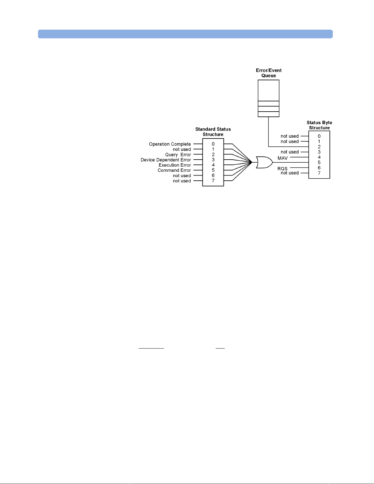
Your programs can monitor the Agilent 86140B series for its operating status, including querying execution or command errors and determining whether or not measurements have been completed. Several status registers and queues are provided to accomplish these tasks as shown in

Figure on page 30. The status structures shown in the figure consist of

condition registers, event registers, event enable registers, and, in the case of the Operation Status Structure, transition filters. For example, there exists the Standard Status Condition Register, the Standard Status Event Register, and the Standard Status Event Enable Register. Condition registers show the current condition of the status lines. Event registers show that an event has occurred. Once latched, these registers stay set until cleared. Event enable registers are masks that you can use to enable or disable the reporting of individual bits from an event register.

Querying a register always returns the value as a weighted sum of all set bits. Refer to Tab l e 5 . For example, if the value returned was 528, this would indicate that bits 4 and 9 were set. Mask registers are set using these same values. For example, the *ESE 60 command sets bits 2 through 5 of the Standard Status Event Enable Register. Whenever any one of bits 2 through 5 of the Standard Status Event Register goes high, bit 5 of the status byte will be set.

Table 5 Decimal Values of Event Enable Register Bits

Bit Decimal Value Bit Decimal Value Bit Decimal Value Bit Decimal Value

0 1 4 16 8 256 12 4096

1 2 5 32 9 512 13 8192

2 4 6 64 10 1024 14 16,384

3 8 7 128 11 2048 15 32,768

Agilent 86140B Optical Spectrum Analyzer, Second Edition 29

Page 30

Remote Operation Monitoring the Instrument

Figure 1 Status Registers

The STATUS:PRESET command clears all event registers and sets all bits in the event enable registers. Use the *CLS common command to clear all event registers and all queues except the output queue. If *CLS is sent immediately following a program message terminator, the output queue is also cleared. In addition, the request for the *OPC bit is also cleared.

For an example program using the status registers, refer to “Example 9.

Monitoring the status registers” on page 56.

Status Byte

The Status Byte contains summary bits that monitor activity in the other status registers and queues. The register’s bits are set and cleared by summary bits from other registers or queues. If a bit in the Status Byte goes high, query the value of the source register to determine the cause.

Command Use

GPIB serial poll command Returns the status byte value. Reads bit 6 as the

Request Service (RQS) bit and clears the bit which clears the SRQ interrupt.

*STB? common command Returns the status byte value. Reads bit 6 as the

Master Summary Status (MSS) and does not clear the bit or have any effect on the SRQ inter rupt.

*SRE common command Sets or reads the event enable register value

(mask).

30 Agilent 86140B Optical Spectrum Analyzer, Second Edition

Page 31

Monitoring the Instrument Remote Operation

Standard Status Structure

The Standard Status Structure monitors the following instrument status events: operation complete, query error, device dependent error, execution error, and command error. When one of these events occurs, the event sets the corresponding bit in the register.

Command Use

*ESR? common command Returns and clears the value of the event register.

*OPC common command When all operations have finished, sets bit 0 of

the event register. The query returns a 1 when all operations have finished.

*ESE common command Sets or returns the value of the event enable reg

ister (mask).

Output Queue

The output queue stores the instrument responses that are generated by certain commands and queries that you send to the instrument. The output queue generates the Message Available Summary bit when the output queue contains one or more bytes. This summary bit sets the MAV bit (bit

4) in the Status Byte. The method used to read the output queue depends

upon the programming language and environment. For example, with BASIC, the output queue may be read using the ENTER statement.

Error Queue

As errors are detected, they are placed in an error queue. Instrument specific errors are indicated by positive values. General errors have negative values. You can clear the error queue by reading its contents, sending the *CLS command, or by cycling the instrument’s power. The error queue is first in, first out. If the error queue overflows, the last error in the queue is replaced with error -350, “Queue overflow.” Any time the queue overflows, the least recent errors remain in the queue, and the most recent error is discarded. The length of the instrument’s error queue is 30 (29 positions for the error messages, and 1 position for the “Queue overflow” message). Querying errors removes the oldest error from the head of the queue, which opens a position at the tail of the queue for a new error. When all the errors have been read from the queue, subsequent error queries return 0, “No error.”

Command Use

*CLS common command Clears the error queue (and all event registers).

EM:ERROR? Returns and removes the oldest error from the

SYST

head of the queue.

Agilent 86140B Optical Spectrum Analyzer, Second Edition 31

Page 32

Remote Operation Amplitude Correction Remote Commands

Amplitude Correction Remote Commands

Multi-Point Amplitude Correction (AMPCOR) gives you the ability to compensate for amplitude errors introduced by optical connectors or cable losses at the input port of a device. For example, if an optical connector or cable is placed between the OSA and an optical component, AMPCOR can compensate for the connector or cable loss. With AMPCOR, amplitude levels (including markers) indicate the power at the optical component’s output. The true characteristics of the device are revealed by moving the measurement (or reference) point beyond the connector or cable to the optical component. Higher measurement accuracy is achieved by eliminating optical connector or cable loss errors.

Correction factors are entered in wavelength and amplitude pairs. The wavelength values entered must be equal or increasing in value to prevent an error condition. If more than one offset is entered for a given wavelength, a step in amplitude can be created. For example, if the following data set was entered into correction set 1:

:SENSE:CORRECTION:CSET1 :SENS

E:CORRECTION:DATA 1200E-9,0,1300E-9,0, 1300E-9,2,1400E-9,4

wavelengths up to and including 1300 nm will have a 0 dB offset. Wavelengths between 1300 nm and 1400 nm will be interpolated between 2 dB and 4 dB (logarithmically or linearly, depending on the setting selection). If more than two offsets are entered for a given wavelength, the first and last offsets entered will be used to correct the trace. Any intermediate points will be disregarded. For example, if the following correction data was entered into correction set 2:

:SENSE:CORRECTION:CSET 2 :SENS

E:CORRECTION:DATA 1200E-9,0,1300E-9,0,1300E-9,5,1300E-9,2,1400E-9,4

the OSA would use the 0 dB offset and the 2 dB offset as correction points and interpolation endpoints, and disregard the 5 dB offset. In normal usage, correction offsets should be continuous, and the wavelengths in increasing order.

Four sets of correction factors are available and stored in memory. Only one set may be selected at a time.

When AMPCOR is turned on, the correction points are applied across the active measurement range and added to all measurement results. Betwe

en points, the correction values are interpolated linearly or logarithmically. When measuring at wavelengths outside the first and last correction points, the first or last value (as appropriate) is used as the

32 Agilent 86140B Optical Spectrum Analyzer, Second Edition

Page 33

Amplitude Correction Remote Commands Remote Operation

correction value. Refer to page 32 for a listing of the AMPCOR remote commands. Since AMPCOR consumes processing power, you should only use AMPCOR if necessary.

Tip: You can turn on amplitude corrections and select a correction set by

pressing AMPLITUDE > AMPLITUDE SETUP from the OSA front panel. Refer to

“Amplitude Setup” on page 3-5 in the User’s Guide for Amplitude Setup

panel information.

The following commands will select correction set number 1, set the correction factor, and turn AMPCOR ON.

:SENSE:CORRECTION:CSET 1 :SENS

E:CORRECTION:DATA 1200E-9,0,1201E-9,2, 1202E-9,3,1203E-9,0

:SENS

E:CORRECTION:STATE ON

The following commands will enter values to correction set number 2, 3, and 4.

:SENSE:CORRECTION:CSET 2 :SENS

E:CORRECTION:DATA 1200E-9,0,1201E-9,1, 1202E-9,2,1203E-9,0

:SENS

E:CORRECTION:CSET 3

:SENS

E:CORRECTION:DATA 1200E-9,0,1201E-9,2, 1202E-9,3,1203E-9,0

NOTE

:SENS

E:CORRECTION:CSET 4

:SENS

E:CORRECTION:DATA 1200E-9,0,1201E-9,1, 1202E-9,3,1203E-9,0

While AMPCOR is ON, selecting a different correction set will immediately correct the measured data to the new correction set. For example, to select correction set number three use:

:SENS:CORR:CSET 3

If AMPCOR is used when auto-ranging is turned OFF, the signal may get clipped. To avoid signal clipping, limit the correction factor to a range from –3dB to +12dB.

Agilent 86140B Optical Spectrum Analyzer, Second Edition 33

Page 34

Remote Operation Techniques to Improve Throughput

Techniques to Improve Throughput

This section provides a series of suggestions and rules of thumb that are useful in increasing measurement throughput.

Take control of the sweep

Put the instrument in single sweep mode using INIT:CONT:OFF, and sweep only to acquire data. The sweep is the most time consuming operation in the OSA. You should send all your sweep related settings and then take the sweep, taking as few sweeps as possible.

Turn the display off

The single most effective thing you can do to increase measurement throughput is turn the display off. If the operator is interacting with the computer display rather than the instrument display, consider turning the display off. This does not make the internal motors or the data acquisition system operate any faster. Instead, it removes all the OSA system overhead associated with maintaining a real time display. This makes software intensive operations much faster, but sweep associated operations won’t change very much. As a result, the speed improvement you will see depends on your application. With the display off, you can expect a typical application that is taking sweeps, using markers and transferring traces to run about twice as fast.

To t u rn t h e di s p l a y o f f :

SENDMESSAGE DISP OFF; *OPC? RECEIVEINTEGER

This takes about 12 seconds and does not affect the instrument state. You can turn the display back on whenever you want to, either by sending DISP ON or by pressing the local key on the instrument front panel. It again will take about 12 seconds. Note that you cannot turn off the display from the front panel.

The instrument behavior with the display off is identical to behavior with display on, only faster. You can develop your application with the display on for easy debugging, then turn the display off once everything is working.

The DISP OFF command is unusual in that a *RST or a SYST:PRES does not turn the display back on. Once off, the display stays off until you want it to come back on.

34 Agilent 86140B Optical Spectrum Analyzer, Second Edition

Page 35

Techniques to Improve Throughput Remote Operation

Combine commands into a single message

The instrument will execute commands faster if it receives them all in a single message. For example:

SENDMESSAGE INIT // take a sweep SENDMESSAGE *OPC? // instrument tells us when done RECEIVEINTEGER // wait for reply

This is inefficient because the instrument will receive and parse the INIT command, and actually launch the sweep before returning to GPIB to receive and parse the *OPC?. The instrument will hold off GPIB for several hundred milliseconds before accepting the *OPC? message. Instead, combine them into a single message:

SENDMESSAGE INIT;OPC? // take a sweep, instrument tells us when

done

RECEIVERINTEGER // wait for reply

A good rule of thumb is to combine closely related commands. For example, sending the OPC with the command it waits for makes good sense. If you are only changing one or two sweep parameters, you might include that in the message also. Avoid putting too much in a single message, as this makes it difficult to read and rearrange your application program contents.

Transfer traces with more than 2 marker operations

Modern controllers have plenty of processing power to calculate trace statistics, and can often calculate faster than the instrument. The rule of thumb is that if you perform more than two marker functions (and associated value read back), it is more efficient to transfer the trace and do the post-processing in your computer. It takes about 1/4 second to transfer a 1000 point trace using a 32 bit binary transfer.

The primary exception to this rule is the noise markers. The noise markers use the actual resolution bandwidth (measured on an instrument-byinstrument basis) to normalize the measured power to a 1 or 0.1 nm span. This calculation is difficult to perform in the controller because it doesn’t have direct access to the actual resolution bandwidth values.

Use 32 bit binary trace transfers

The most convenient trace transfer is an ASCII trace transfer, but downloading the data in REAL32 format is substantially faster. Binary can take half as long as ASCII, which saves about 100 ms for every 1000 points transferred. ASCII format sends the trace value reformatted as 12 character strings, whereas a 32 bit binary transfer sends the data in IEEE 32 bit format. This is the same representation used inside the instrument and takes only 4 8-bit data bytes. There are two binary transfer formats

Agilent 86140B Optical Spectrum Analyzer, Second Edition 35

Page 36

Remote Operation Techniques to Improve Throughput

available - IEEE 32 bit and IEEE 64 bit formats. The instrument does not carry more than 32 bits of data resolution internally, so there is no benefit to doing a 64 bit transfer. To configure for a 32 bit binary transfer:

SENDMESSAGE FORMAT REAL,32

The advantage of binary over ASCII can be even greater for automation projects using Visual Basic and C++. With short binary transfer times, the data transfer process is faster than the hardware. This makes it possible to devise ways to process the data faster to keep up with the hardware. Note that in Visual C++ it is possible to download and convert the trace in one step by changing the format string.

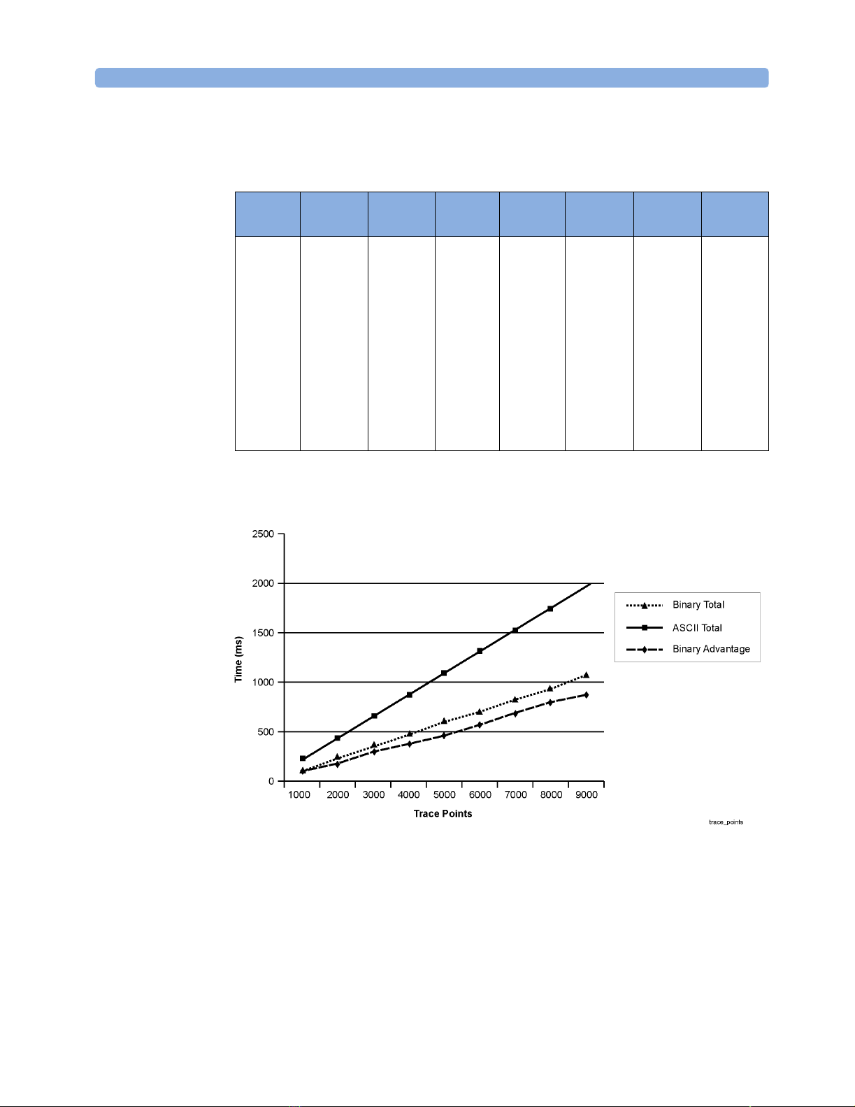
The following table and chart compare the different times it takes to transfer trace data. The data was taken using Visual C++ with National Instruments VISA. Since the data must be converted to be useful, both transfer and conversion times are listed.

36 Agilent 86140B Optical Spectrum Analyzer, Second Edition

Page 37

Techniques to Improve Throughput Remote Operation

Table 6 Binary vs. ASCII Downloads

Trace Points

1000 47 78 125 219 16 235 110

2000 79 171 250 422 16 438 188

3000 110 250 360 640 31 671 311

4000 140 344 484 844 31 875 391

5000 172 437 609 1063 31 1094 485

6000 203 515 718 1282 31 1313 595

7000 234 594 828 1484 47 1531 703

8000 266 687 953 1703 63 1766 813

9000 297 781 1078 1906 63 1969 891

Binary

Transfer

Binary

Conversion

Binary Total

ASCII

Transfer

ASCII

Conversion

ACSII Total

Binary

Advantage

Figure 2 Binary vs. ASCII Downloads

Agilent 86140B Optical Spectrum Analyzer, Second Edition 37

Page 38

Remote Operation Techniques to Improve Throughput

One of the biggest challenges to transferring binary data on a Windows platform is the necessity to swap the byte order. For a 32 bit floating point number, you have 4 bytes. If we number them 0, 1, 2, and 3, we need to swap 0 and 3 and then swap 1 and 2. The C algorithm below does this:

INT CNT; CHAR TEMPBYTE; CHAR *TRACEBYTES;

// allocate buffer and transfer trace into traceBytes

FOR (CNT=0;CNT<NUMBYTES;CNT+=4)

{

// swap bytes 3 and 0

TEMPBYTE = TRACEBYTES[CNT]; TRACEBYTES[CNT] = TRACEBYTES[CNT + 3]; TRACEBYTES[CNT+3] = TEMPBYTE;

// swap bytes 2 and 1

TEMPBYTE = TRACEBYTES[CNT+1]; TRACEBYTES[CNT+1] = TRACEBYTES[CNT+2]; TRACEBYTES[CNT+2] = TEMPBYTE;

}

Because of the type casting and byte manipulation involved, it is very difficult to do this in Visual Basic. It is possible to write a DLL in Visual C to do the conversion.

Optimize Sweep Parameters

It is common practice to use conservative sweep parameters when first developing a test, perhaps sweeping broader or using narrower resolution bandwidth than necessary, to get reliable data. Once the application is running reliably, evaluate your sweep settings:

• Consider a wider resolution bandwidth.

• Consider a narrower span.

• Consider taking one larger sweep instead of several small ones.

• Set sensitivity at a higher level.

• Experiment with sweep time.

• Take as few sweeps as possible to obtain test data.

38 Agilent 86140B Optical Spectrum Analyzer, Second Edition

Page 39

Sending Remote Commands over the LAN Remote Operation

Sending Remote Commands over the LAN

The Standard Instrument Control Library (SICL) Local Area Network (LAN) enables you to control your remote analyzer over the LAN as if your local analyzer is connected directly to the controller with the GPIB. SICL provides control of your analyzer over the LAN, using a variety of computing platforms, I/O interfaces, and operating systems.

Your analyzer implements a SICL LAN server. To control the analyzer, you need a SICL LAN client application running on a computer or workstation that is connected to the analyzer over a LAN. Typical applications implementing a SICL LAN client include:

• Agilent VEE

•HT BASIC

• National Instrument’s LabView with Agilent VISA/SICL client drivers

SICL LAN can be used with Windows 95, Windows 98, Windows NT, and HP-UX.

Agilent 86140B Optical Spectrum Analyzer, Second Edition 39

Page 40

Remote Operation Sending Remote Commands over the LAN

SICL LAN Set-up Information

Before setting up your controller as a SICL LAN client, you will need to collect the following information:

GPIB name The GPIB name is the name given to a device used to

communicate with the analyzer. Your analyzer is shipped with hpib7 as the GPIB name.

GPIB logical unit

GPIB device address

The SICL LAN client uses the GPIB name, GPIB logical unit number, and GPIB address to communicate with the server. You must match these parameters exactly when you set up the SICL LAN client and server.

The logical unit number is a unique integer assigned to the device to be controlled using SICL LAN. Your analyzer is shipped with the logical unit number set to 7.

The device address is the GPIB device address (bus address) assigned to the device to be controlled using SICL LAN. Your analyzer is shipped with the GPIB device address set to 23.

Setting Up Your Analyzer as a SICL LAN Server

Your analyzer becomes an active SICL LAN server when configured for networking. Please refer to “SICL LAN Set-up Information” on page 40 for the network setup information. See “To change the GPIB address´´ on

page 18 to change the GPIB address from the front panel.

40 Agilent 86140B Optical Spectrum Analyzer, Second Edition

Page 41

Sending Remote Commands over the LAN Remote Operation

Setting Up Your Controller as a SICL LAN Client

For Windows 95, Windows 98, and Windows NT:

1 Install Agilent I/O Libraries.

2 Run I/0 configuration.

3 Select LAN Client from the Available Interface Types.

4 Click Configure.

5 Click OK.

6 Select VISA LAN Client from the Available Interface Types.

7 Click Configure.

8 Enter the hostname or IP address of your analyzer.

9 Enter hpib7 in the remote SICL interface name field. 10 Click OK. 11 Select the new VISA LAN Client then click Edit.

12 Click Edit VISA Config.

13 Clear the Unselect Identify devices at run-time check box.

14 Click Add Device.

15 Enter the GPIB address of your analyzer, then Click OK three times to exit the

application.

For HPUX:

1 Install Agilent SICL Libraries.

2 Run iosetup.

3 Select LAN Client from the Available Interface Types.

4 Click Configure.

5 Click OK.

Limitations:

1 The re m ay be a perio d of u p to 5 second s when yo u will be una ble to op en a LAN

interface with the OSA. It is common for LAN clients to open an Interface Session for device actions. If your client application opens an interface session, there will be a delay between the time the interface is closed and when you will be able to open a new interface.

Agilent 86140B Optical Spectrum Analyzer, Second Edition 41

Page 42

Remote Operation Sending Remote Commands over the LAN

2 You will receive separate responses to SCPI queries that are combined on a

single line. For example if you send SENS:START?STOP? you will have to read twice to get both responses.

iprintf (osa, “SENS:START?;STOP?\n”); iscanf (osa, “%t”, startWavelength); /* +6.00000000E-007 */ iscanf (osa, “%t”, stopWavelength); /* +1.70000000E-006 */

Normally (with GPIB) you would receive both responses separated with a semicolon.

iprintf (osa, “SENS:START?;STOP?\n”); iscanf (osa, “%t”, startStop); /* +6.00000000E-007;+1.70000000E-006 */

3 You must not set a time-out of less then 1-second.

42 Agilent 86140B Optical Spectrum Analyzer, Second Edition

Page 43

Example Programs Remote Operation

Example Programs

These programs are provided to give you examples of using Agilent 86140B series remote programming commands in typical applications. They are not meant to teach general programming techniques or provide ready-to-use solutions. They should allow you to see how measurements are performed and how to return data to the computer. The programs are written in BASIC for Windows.

The following example programs are provided in this section:

Example 1. Initialization and a simple measurement . . . . . . . .44

Example 2. Locating the largest signal . . . . . . . . . . . . . . . . . . . .46

Example 3. Bandwidth . . . . . . . . . . . . . . . . . . . . . . . . . . . . . . . . . .47

Example 4. Maximum and minimum amplitude values. . . . . . .49

Example 5. Maximum and minimum values over time . . . . . . .51

Example 6. Returning trace data. . . . . . . . . . . . . . . . . . . . . . . . . .52

Example 7. Trace normalization . . . . . . . . . . . . . . . . . . . . . . . . . .54

Example 8. Total power measurement. . . . . . . . . . . . . . . . . . . . .55

Example 9. Monitoring the status registers . . . . . . . . . . . . . . . .56

Example 10 SMSR calculation with display off . . . . . . . . . . . . .58

Agilent 86140B Optical Spectrum Analyzer, Second Edition 43

Page 44

Remote Operation Example Programs

Example 1. Initialization and a simple measurement

Description

This program provides the basic building block for beginning development of a measurement routine. The *RST common command resets the instrument to predetermined settings to provide a common starting point. The automeasure function locates the largest signal in the spectrum and optimizes the display of the signal. The maximum signal is located and a marker placed on the signal. This signal is then used for the autoalign function. Autoalign aligns the internal components of the OSA to compensate for any effects of handling, temperature, and humidity. This operation should be performed whenever the instrument is moved or the environmental conditions change. It should be performed after the instrument is at operating temperature. Periodic use of autoalign assures optimum performance. The program sets the start and stop wavelength and the amplitude sensitivity.

Program

! Initialization and a simple measurement ! PRINT "Single Measurement Example" CLEAR 7 ! Clear GPIB interface ASSIGN @Osa TO 723;EOL CHR$(10) END ! Turn on END message CLEAR @Osa ! Selected device clear OUTPUT @Osa;"disp:wind:text:data 'Single Measurement'" ! !******************************Initialization Routine****************************** ! PRINT PRINT "Presetting the instrument" OUTPUT @Osa;"*rst;*opc?" ENTER @Osa;Temp ! PRINT "Turning buffer on" OUTPUT @Osa;"syst:comm:gpib:buff on" ! Turn OSA GPIB input buffer on ! PRINT PRINT "Performing AutoMeasure" ! Automeasure OUTPUT @Osa;"disp:wind:trac:all:scal:auto;*Opc?" ENTER @Osa;Temp ! PRINT "Performing Autoalign" ! Autoalign OUTPUT @Osa;"cal:alig:mark1;*opc?" ENTER @Osa;Temp ! !**************************************************************************** ! PRINT PRINT "...measurement begins" ! OUTPUT @Osa;"sens:wav:star 1314nm" ! Set start wavelength OUTPUT @Osa;"sens:wav:stop 1316nm" ! Set stop wavelength OUTPUT @Osa;"sens:pow:dc:rang:low -70dbm" ! Set amplitude sensitivity OUTPUT @Osa;"sens:bwid:res 0.1nm" ! Set the resolution bandwidth OUTPUT @Osa;"init:imm;*opc?" ! Take a sweep ENTER @Osa;Temp OUTPUT @Osa;"calc:mark1:max" ! Locate max signal

44 Agilent 86140B Optical Spectrum Analyzer, Second Edition

Page 45

Example Programs Remote Operation

OUTPUT @Osa;"calc:mark1:scen" ! Marker to center OUTPUT @Osa;"init:imm;*opc?" ! Take a sweep ENTER @Osa;Temp ! LOCAL @Osa ! Return to local operation END

Agilent 86140B Optical Spectrum Analyzer, Second Edition 45

Page 46

Remote Operation Example Programs

Example 2. Locating the largest signal

Description

This program finds the largest signal, zooms to a narrow span, and then uses markers to return signal wavelength and amplitude to the computer.

Program

! Locating the Largest Signal ! PRINT "OSA Zoom Example" CLEAR 7 ! Clear GPIB interface ASSIGN @Osa TO 723;EOL CHR$(10) END ! Turn on END message CLEAR @Osa ! Selected device clear OUTPUT @Osa;"disp:wind:text:data 'Display the largest Signal'" ! PRINT PRINT "Presetting the instrument" OUTPUT @Osa;"*rst;*opc?" ! Preset the instrument ENTER @Osa;Temp PRINT ! PRINT "Turning buffer on" OUTPUT @Osa;"syst:comm:gpib:buff on" ! Turn OSA GPIB input buffer on ! PRINT PRINT "Performing AutoMeasure" ! Automeasure OUTPUT @Osa;"disp:wind:trac:all:scal:auto;*opc?" ENTER @Osa;Temp ! PRINT "Performing Autoalign" ! Autoalign OUTPUT @Osa;"cal:alig:mark1;*opc?" ENTER @Osa;Temp ! PRINT "...Measurement begins" ! OUTPUT @Osa;"init:imm;*opc?" ! Take a sweep, wait for completion ENTER @Osa;Temp OUTPUT @Osa;"calc1:mark1:max" ! Marker to peak OUTPUT @Osa;"calc1:mark1:scen" ! Marker to center OUTPUT @Osa;"sens:wav:span 10nm" ! Set span ! OUTPUT @Osa;"init:imm;*opc?" ! Take a sweep, wait for completion ENTER @Osa;Temp OUTPUT @Osa;"calc1:mark1:max" ! Marker to peak OUTPUT @Osa;"calc1:mark1:scen" ! Marker to center ! OUTPUT @Osa;"init:imm;*opc?" !Take a sweep, wait for completion ENTER @Osa;Temp ! OUTPUT @Osa;"calc1:mark1:x?" ! Read marker wavelength ENTER @Osa;Markwl ! OUTPUT @Osa;"calc1:mark1:y?" ! Read marker amplitude ENTER @Osa;Markamp ! PRINT PRINT "Marker values:" Markwl=Markwl*1.E+9 ! Convert to nm PRINT "wavelength: ",Markwl;"nm" PRINT "amplitude: ",Markamp;"dBm" ! LOCAL @Osa ! Return OSA to local operation END

46 Agilent 86140B Optical Spectrum Analyzer, Second Edition

Page 47

Example Programs Remote Operation

Example 3. Bandwidth

Description

The 20 dB marker BW function is used to determine the bandwidth of the signal. The program assumes a narrowband signal as an input.

Program

! Bandwidth ! CLEAR 7 ! Clear GPIB interface ASSIGN @Osa TO 723;EOL CHR$(10) END ! Turn on END message CLEAR @Osa ! Selected device clear PRINT "Signal Bandwidth Measurement" OUTPUT @Osa;"disp:wind:text:data 'Signal Bandwidth Measurement'" ! PRINT PRINT "Presetting the instrument" OUTPUT @Osa;"*rst;*opc?" ! Preset the instrument ENTER @Osa;Temp ! PRINT "Turning buffer on" OUTPUT @Osa;"syst:comm:gpib:buff on" ! Turn OSA GPIB input buffer on ! PRINT "...Measurement Begins" ! OUTPUT @Osa;"sens:wav:star 1530nm" ! Set start wavelength OUTPUT @Osa;"sens:wav:stop 1570nm" ! Set stop wavelength OUTPUT @Osa;"sens:pow:dc:rang:low -60dBm" ! Set sensitivity OUTPUT @Osa;"init:imm;*opc?" ! Take a sweep ENTER @Osa;Temp ! OUTPUT @Osa;"calc1:mark1:max" ! Marker to peak OUTPUT @Osa;"calc1:mark1:srl" ! Marker to reference level OUTPUT @Osa;"calc1:mark1:scen" ! Marker to center OUTPUT @Osa;"sens:wav:span 10nm" ! Set span ! OUTPUT @Osa;"calc1:mark1:x?" ! Read marker wavelength ENTER @Osa;Markwl OUTPUT @Osa;"calc1:mark1:y?" ! Read marker amplitude ENTER @Osa;Markamp Markwl=Markwl*1.E+9!Convert to standard measurement units (nm) PRINT "Marker wavelength";Markwl;"nm" PRINT "Marker amplitude";Markamp;"dBm" PRINT ! OUTPUT @Osa;"sens:bwid:res 0.1 nm" ! Set resolution bandwidth to min OUTPUT @Osa;"sens:wav:span 2nm" ! Set span OUTPUT @Osa;"init:imm;*opc?" ! Take a sweep ENTER @Osa;Temp ! OUTPUT @Osa;"calc1:mark1:max" ! Marker to peak for reference point OUTPUT @Osa;"calc1:mark1:func:bwid:ndb -20.0 db" ! Select db down where bw is calculated OUTPUT @Osa;"calc1:mark1:func:bwid:int on" ! Enable bw marker interpolation OUTPUT @Osa;"calc1:mark1:func:bwid:read wav" ! Set the BW unit of measurement to WL OUTPUT @Osa;"calc1:mark1:func:bwid:stat on" ! Enable bandwidth marker ! OUTPUT @Osa;"calc1:mark1:func:bwid:res?" ! Return axis values between markers ENTER @Osa;Rbw IF Rbw<9.E+37 THEN Cnt! test for valid result PRINT "BW not found" STOP

Agilent 86140B Optical Spectrum Analyzer, Second Edition 47

Page 48

Remote Operation Example Programs

Cnt:! label ! OUTPUT @Osa;"calc1:mark1:func:bwid:x:left?" ! Read left BW marker X axis value ENTER @Osa;Markleft OUTPUT @Osa;"calc1:mark1:func:bwid:x:righ?" ! Read right BW marker X axis value ENTER @Osa;Markright OUTPUT @Osa;"calc1:mark1:func:bwid:x:cent?" ! Read center BW marker X axis value ENTER @Osa;Markcent ! ! Convert to standard measurement units (nm) Rbw=Rbw*1.E+9 Markleft=Markleft*1.E+9 Markright=Markright*1.E+9 Markcent=Markcent*1.E+9 ! PRINT "-20 db Marker bandwidth",Rbw;"nm" PRINT "Left marker";Markleft;"nm" PRINT "Right marker";Markright;"nm" PRINT "Center";Markcent;"nm"

LOCAL @Osa END

48 Agilent 86140B Optical Spectrum Analyzer, Second Edition

Page 49

Example Programs Remote Operation

Example 4. Maximum and minimum amplitude values

Description

The marker delta function is used to find the maximum and minimum (peak and pit) values of the signal.

Program

! Maximum and Minimum amplitude values ! CLEAR 7 ! Clear GPIB interface ASSIGN @Osa TO 723;EOL CHR$(10) END ! Turn on END message CLEAR @Osa ! Selected device clear ! PRINT "Peak to Pit Example" OUTPUT @Osa;"disp:wind:text:data 'Minimum and Maximum Signals'" ! PRINT PRINT "Presetting the instrument" OUTPUT @Osa;"*rst;*opc?" ! Preset the instrument ENTER @Osa;Temp ! PRINT "Turning buffer on" OUTPUT @Osa;"syst:comm:gpib:buff on" ! Turn OSA GPIB input buffer on ! OUTPUT @Osa;"sens:wav:star 1530nm" ! Set start wavelength OUTPUT @Osa;"sens:wav:stop 1570nm" ! Set stop Wavelength OUTPUT @Osa;"init:imm;*opc?" ! Take a sweep ENTER @Osa;Temp OUTPUT @Osa;"calc1:mark1:max" ! Marker to peak OUTPUT @Osa;"calc1:mark1:scen" ! Marker to center OUTPUT @Osa;"calc:mark1:srl" ! Marker to reference level OUTPUT @Osa;"sens:wav:span 10nm" ! Set span ! PRINT "Measurement begins" PRINT ! OUTPUT @Osa;"sens:pow:dc:rang:low -60dBm" ! Set sensitivity OUTPUT @Osa;"init:imm;*opc?" ! Take a sweep ENTER @Osa;Temp ! OUTPUT @Osa;"calc1:mark1:max" ! Marker to peak OUTPUT @Osa;"calc1:mark1:x?" ! Read marker wavelength ENTER @Osa;Markwl OUTPUT @Osa;"calc1:mark1:y?" ! Read marker amplitude ENTER @Osa;Markamp ! OUTPUT @Osa;"calc1:mark1:func:delt:stat on" !Turn delta marker on ! OUTPUT @Osa;"calc1:mark1:min" ! Marker to pit ! OUTPUT @Osa;"calc1:mark1:func:delt:y:offs?" ! Read Delta Y marker ENTER @Osa;Markdelty OUTPUT @Osa;"calc1:mark1:func:delt:x:offs?" ENTER @Osa;Markdeltx ! PRINT " Marker values" PRINT Markwl=Markwl*1.E+9 ! Convert to nm PRINT Markwl;"nm",Markamp;"dBm" ! Markdeltx=Markdeltx*1.E+9 ! Convert to nm

Agilent 86140B Optical Spectrum Analyzer, Second Edition 49

Page 50

Remote Operation Example Programs

! PRINT PRINT "Marker Delta Values" PRINT PRINT Markdeltx;"nm",Markdelty;"dBm" ! LOCAL @Osa ! Return control to local END

50 Agilent 86140B Optical Spectrum Analyzer, Second Edition

Page 51

Example Programs Remote Operation

Example 5. Maximum and minimum values over time

Description

This program locates the largest signal using automeasure, and adjusts the center wavelength, span, and sensitivity settings. Trace B is then viewed and updated and set to maximum hold. Trace C is then viewed, updated, and set to minimum hold. Signal variations with time can now be monitored.

Program

! Maximum and minimum values over time ! CLEAR 7 ! Clear GPIB interface ASSIGN @Osa TO 723;EOL CHR$(10) END ! Turn on END message CLEAR @Osa ! Selected device clear ! PRINT "Min/Max Hold Example" OUTPUT @Osa;"disp:wind:text:data 'Minimum and Maximum Signals'" ! PRINT PRINT "Presetting the instrument" OUTPUT @Osa;"*rst;*opc?" ! Preset the instrument ENTER @Osa;Temp ! PRINT "Turning buffer on" OUTPUT @Osa;"syst:comm:gpib:buff on" ! Turn OSA GPIB input buffer on ! PRINT "...measurement begins" ! OUTPUT @Osa;"sens:wav:star 1530nm" ! Set start wavelength OUTPUT @Osa;"sens:wav:stop 1570nm" ! Set stop Wavelength OUTPUT @Osa;"init:imm;*opc?" ! Take a sweep ENTER @Osa;Temp OUTPUT @Osa;"calc1:mark1:max" ! Marker to peak OUTPUT @Osa;"calc1:mark1:scen" ! Marker to center OUTPUT @Osa;"calc:mark1:srl" OUTPUT @Osa;"sens:wav:span 20nm" ! Set span ! OUTPUT @Osa;"sens:pow:dc:rang:low -65dBm" ! Set the sensitivity ! ! Update and view trace B and set it to max hold ! OUTPUT @Osa;"disp:wind:trac:stat trB, on" ! View trace B OUTPUT @Osa;"trac:feed:cont trB, Alw" ! Update trace B OUTPUT @Osa;"calc2:max:stat on” ! Set trace B to max hold ! ! Update and view trace C and set it to min hold ! OUTPUT @Osa;"disp:wind:trac:stat trC, on" ! View trace C OUTPUT @Osa;"trac:feed:cont trC, Alw" ! Update trace C OUTPUT @Osa;"calc3:min:stat on" ! Set trace C to min hold ! OUTPUT @Osa;"init:cont on" ! Turn continuous sweep on ! LOCAL @Osa ! Return to local control END

Agilent 86140B Optical Spectrum Analyzer, Second Edition 51

Page 52

Remote Operation Example Programs

Example 6. Returning trace data

Description

This program locates the largest signal and then zooms to a narrow span. The trace length is changed to 101 points and the entire trace data is read in and printed on the display.

Program

! Returning trace data ! CLEAR 7 ! Clear GPIB interface ASSIGN @Osa TO 723;EOL CHR$(10) END ! Turn on END message CLEAR @Osa ! Selected device clear ! PRINT "OSA Trace Example" OUTPUT @Osa;"disp:wind:text:data 'Trace Readout'" ! DIM Tdata(1:101) ! Create a trace array DIM Wdata(1:101) ! Wavelength data ! PRINT PRINT "Presetting the instrument" OUTPUT @Osa;"*rst;*opc?" ! Preset the instrument ENTER @Osa;Temp ! PRINT "Turning buffer on" OUTPUT @Osa;"syst:comm:gpib:buff on" ! Turn OSA GPIB input buffer on ! OUTPUT @Osa;"sens:wav:star 1530nm" ! Set start wavelength OUTPUT @Osa;"sens:wav:stop 1570nm" ! Set stop Wavelength OUTPUT @Osa;"init:imm;*opc?" ! Take a sweep ENTER @Osa;Temp OUTPUT @Osa;"calc1:mark1:max" ! Marker to peak OUTPUT @Osa;"calc1:mark1:scen" ! Marker to center OUTPUT @Osa;"calc:mark1:srl" ! Marker to reference level ! PRINT "Measurement begins" ! OUTPUT @Osa;"sens:wav:span 10nm" ! Set span OUTPUT @Osa;"init:imm;*opc?" ENTER @Osa;Temp OUTPUT @Osa;"calc1:mark1:max" ! Marker to peak OUTPUT @Osa;"calc1:mark1:scen" ! Marker to center OUTPUT @Osa;"init:imm;*opc?" ! Take a sweep ENTER @Osa;Temp ! ! Read in the trace data ! OUTPUT @Osa;"sens:swe:poin 101" ! Set trace length to 101 OUTPUT @Osa;"init:imm;*Opc?" ! Take a sweep ENTER @Osa;Temp ! ! !OUTPUT @Osa;"form ascii" ! Set data format to ASCII OUTPUT @Osa;"trac:data:y? tra" ! Request data ENTER @Osa;Tdata(*) ! Read trace data ! ! Read start, stop and trace length ! OUTPUT @Osa;"sens:wav:star?" ! Read start wavelength ENTER @Osa;Startw OUTPUT @Osa;"sens:wav:stop?" ! Read stop wavelength

52 Agilent 86140B Optical Spectrum Analyzer, Second Edition

Page 53

Example Programs Remote Operation

ENTER @Osa;Stopw OUTPUT @Osa;"sens:swe:poin?" ! Read trace length ENTER @Osa;Tlength Bucket=(Stop-Start)/(Tlength-1) ! Calculate bucket length PRINT "Data Point Size",Bucket;"nm" ! PRINT "Point","Wavelength","Amplitude" ! ! The following lines calculate the wavelength value of each point of the trace. ! Note that wavelength values of a trace cannot be directly queried. ! FOR I=1 TO 101

Wlength=Startw+(Bucket*(I-1))! Calculate point wavelength Wlength=Wlength*1.E+9 ! Convert to nm PRINT I,Wlength,Tdata(I)

NEXT I ! LOCAL @Osa ! Return to local control END

Agilent 86140B Optical Spectrum Analyzer, Second Edition 53

Page 54

Remote Operation Example Programs

Example 7. Trace normalization

Description

This program demonstrates trace normalization. Normalization is used to observe changes to a displayed response. For example, run the program and then bend the fiber to observe the change in signal level across the spectrum. Trace C displays the difference between trace A and trace B.

Program

! Trace Normalization ! CLEAR 7 ! Clear GPIB interface ASSIGN @Osa TO 723;EOL CHR$(10) END ! Turn on END message CLEAR @Osa ! Selected device clear ! PRINT "OSA Normalization Example" OUTPUT @Osa;"disp:wind:text:data 'OSA Normalization Example'" ! PRINT PRINT "Presetting the instrument" OUTPUT @Osa;"*rst;*opc?" ! Preset the instrument ENTER @Osa;Temp ! PRINT "Turning buffer on" OUTPUT @Osa;"syst:comm:gpib:buff on" ! Turn OSA GPIB input buffer on ! OUTPUT @Osa;"init:imm;*opc?" ENTER @Osa;Temp OUTPUT @Osa;"calc1:mark1:max" ! Marker to peak OUTPUT @Osa;"calc1:mark1:scen" ! Marker to center OUTPUT @Osa;"calc:mark1:srl" ! Marker to reference level OUTPUT @Osa;"calc:mark1:stat off" ! Turn marker 1 off ! PRINT "...Measurement begins" ! OUTPUT @Osa;"Sens:bwid:res 10nm" ! Fix resolution bw ! OUTPUT @Osa;"init:imm;*opc?" ! Take a sweep ENTER @Osa;Temp ! ! Trace A is the active trace OUTPUT @Osa;"Disp:Wind:Trac:Stat TrA,On" ! Turn on Trace A OUTPUT @Osa;"Trac:Feed:Cont TrA, Alw" ! ! Trace B is the reference trace OUTPUT @Osa;"disp:Wind:Trac:Stat TrB,ON" ! Turn on Trace B OUTPUT @Osa;"Trac:Feed:Cont TrB, Alw" ! ! Trace C displays the difference between A & B OUTPUT @Osa;"disp:Wind:Trac:Stat TrC,ON" ! Turn on Trace C OUTPUT @Osa;"Trac:Feed:Cont TrC, Alw"! ! OUTPUT @Osa;"Trac:Feed:Cont TrB,Nev" ! Stop updating B ! OUTPUT @Osa;"init:cont on" ! Set up continuous sweep ! ! Trace math function Log Math C=A-B OUTPUT @Osa;"Calc3:Math:Expr ( TRA/TRB )" ! Normalize Trace A to B OUTPUT @Osa;"Calc3:Math:Stat On" ! Turn on normalization ! LOCAL @Osa ! Return to local control END

54 Agilent 86140B Optical Spectrum Analyzer, Second Edition

Page 55

Example Programs Remote Operation

Example 8. Total power measurement

Description

This program demonstrates the total power function. The ASE broadband noise power of an EDFA source is measured. Two sweeps are taken, one of the entire trace and one, using line markers, of just the noise hump. The total power of the two different traces are displayed.

Program

! Total power measurement ! CLEAR 7 ! Clear GPIB interface ASSIGN @Osa TO 723;EOL CHR$(10) END ! Turn on END message CLEAR @Osa ! Selected device clear ! PRINT PRINT "Presetting the instrument" OUTPUT @Osa;"*rst;*opc?" ! Preset the instrument ENTER @Osa;Temp ! PRINT "Turning buffer on" OUTPUT @Osa;"syst:comm:gpib:buff on" ! Turn OSA GPIB input buffer on ! OUTPUT @Osa;"sens:wav:cent 1550nm" ! Set center wavelength of signal OUTPUT @Osa;"sens:wav:span 10nm" ! Set the span OUTPUT @Osa;"sens:bwid:res .1nm" ! Set resolution bandwidth OUTPUT @Osa;"sens:pow:rang:low -60dbm" ! Set sensitivity to -60 dBm ! OUTPUT @Osa;"init:imm;*opc?" ! Take a sweep ENTER @Osa;Temp ! OUTPUT @Osa;"calc1:tpow:stat 1" ! Turn the power state on OUTPUT @Osa;"calc1:tpow:data?" ! Query the total power ENTER @Osa;Tpower PRINT "Entire trace:";Tpower ! Print the total power PRINT ! ! Select portion of trace OUTPUT @Osa;"calc1:tpow:iran:low 1547.6nm" ! Set the upper & lower OUTPUT @Osa;"calc1:tpow:iran:upp 1552.6nm" ! limits for the calculation ! OUTPUT @Osa;"calc1:tpow:data?" ! Query the total power ENTER @Osa;Tpower PRINT "Portion of trace:";Tpower ! Print the total power ! LOCAL @Osa ! Return to local operation END

Agilent 86140B Optical Spectrum Analyzer, Second Edition 55

Page 56

Remote Operation Example Programs

Example 9. Monitoring the status registers

Description

This program presets the instrument and then selects the largest signal in the span. This program demonstrates the use of status registers to detect programming errors. A serial poll is performed to read the instrument status byte. The same status byte is read with *STB?. The internal error register is also read and displayed. The error queue is queried to display the error condition.

Program

! Monitoring the status registers ! CLEAR 7 ! Clear GPIB interface ASSIGN @Osa TO 723;EOL CHR$(10) END ! Turn on END message CLEAR @Osa ! Selected device clear ! PRINT "OSA Status Byte example" OUTPUT @Osa;"disp:wind:text:data 'OSA Status Byte Example'" PRINT !******************************Initialization routine****************************** ! PRINT "Presetting the instrument" OUTPUT @Osa;"*rst;*opc?" ! Preset the instrument ENTER @Osa;Temp ! PRINT "Turning buffer on" OUTPUT @Osa;"syst:comm:gpib:buff on" ! Turn OSA GPIB input buffer on ! OUTPUT @Osa;"init:imm;*opc?" ENTER @Osa;Temp OUTPUT @Osa;"calc1:mark1:max" ! Marker to peak OUTPUT @Osa;"calc1:mark1:scen" ! Marker to center OUTPUT @Osa;"calc:mark1:srl" ! Marker to reference level OUTPUT @Osa;"sens:wav:span 20nm" ! Set the Span OUTPUT @Osa;"calc:mark1:stat off" ! Turn marker 1 off ! !******************************End Initialization****************************** ! OUTPUT @Osa;"*CLS" ! Clear Error Queue ! OUTPUT @Osa;"*ESE 32" ! Set Standard Event Enable bit 5 (32) ! OUTPUT @Osa;"init:imm;*opc?" ! Take a sweep ENTER @Osa;Temp ! Sbyte=SPOLL(@Osa) ! Read serial poll status byte PRINT PRINT "Serial Poll Status Byte";Sbyte PRINT ! OUTPUT @Osa;"*stb?" ! Read the Status Byte Register ENTER @Osa;Stat PRINT "Status Byte Register:";Stat PRINT ! OUTPUT @Osa;"*esr?" ! Read and clear the Std Event Status Register ENTER @Osa;Stat PRINT "Standard Event Status Register:";Stat PRINT

56 Agilent 86140B Optical Spectrum Analyzer, Second Edition

Page 57

Example Programs Remote Operation

! REPEAT OUTPUT @Osa;"system:error?" ! Query error queue entries ENTER @Osa;Errno;Error$ PRINT "Error Queue";Errno;Error$ UNTIL Errno=0 !Error=0 is end of error queue ! LOCAL @Osa ! Return to local operation END

Agilent 86140B Optical Spectrum Analyzer, Second Edition 57

Page 58

Remote Operation Example Programs

Example 10 SMSR calculation with display off

Description

This program calculates the side mode suppression ratio with the display off.

Program

! SMSR calculation with display off ! CLEAR 7 ! Clear GPIB interface ASSIGN @Osa TO 723;EOL CHR$(10) END ! Turn on END message CLEAR @Osa ! Selected device clear ! PRINT "SMSR example with display off" OUTPUT @Osa;"disp:wind:text:data 'SMSR Measurement'" ! !******************************Initialization Routine****************************** PRINT "Turning display off" OUTPUT @Osa;"disp:wind off;*opc?" ! Turn display off ENTER @Osa;Temp ! PRINT PRINT "Presetting the instrument" OUTPUT @Osa;"*rst;*opc?" ENTER @Osa;Temp ! PRINT "Turning buffer on" OUTPUT @Osa;"syst:comm:gpib:buff on" ! Turn OSA GPIB input buffer on ! ! assumes a light source at approx 1550 nm OUTPUT @Osa;"SENS:WAV:CENT 1550nm" ! Set center to 1550 nm OUTPUT @Osa;"SENS:WAV:SPAN 20nm" ! Set span to 20 nm OUTPUT @Osa;"INIT:IMM;*opc?" ! Take a sweep ENTER @Osa;Temp ! OUTPUT @Osa;"CALC:MARK:MAX" ! Place marker one at Max OUTPUT @Osa;"CALC:MARK:SCEN" ! Set marker to center OUTPUT @Osa;"CALC:MARK:SRL" ! Set marker to reference level OUTPUT @Osa;"SENS:POW:DC:RANGe:LOW -61DBM" ! Set sensitivity to -61 dBm OUTPUT @Osa;"INIT:IMM;*opc?" ! Take a sweep ENTER @Osa;Temp OUTPUT @Osa;"CALC:MARK1:MAX" ! Set marker 1 to Max ! OUTPUT @Osa;"CALC:MARK1:Y?" ! Get the peak amplitude ENTER @Osa;Peakamp OUTPUT @Osa;"CALC:MARK1:MAX:NEXT" ! Set marker 1 to the next highest peak OUTPUT @Osa;"CALC:MARK1:Y?" ! Get amplitude of the next highest peak ENTER @Osa;Nextpeakamp ! PRINT PRINT "Peak Amplitude",Peakamp;"dBm" Smsr=Peakamp-Nextpeakamp ! Calculate Side Mode Suppression mode PRINT "SMSR = ",Smsr ! PRINT PRINT "Turning the display back on" OUTPUT @Osa;"disp:wind on;*Opc?" ! Turn the display back on ENTER @Osa;Temp PRINT "*******Measurement complete*******"

58 Agilent 86140B Optical Spectrum Analyzer, Second Edition

Page 59

Example Programs Remote Operation

LOCAL @Osa ! Return control to OSA END

Agilent 86140B Optical Spectrum Analyzer, Second Edition 59

Page 60

Remote Operation Front Panel Functions to Remote Commands

Front Panel Functions to Remote Commands

This is a table of the front-panel functions of the Agilent 86140B series and the corresponding remote commands.

Table 7 Front Panel Function to Remote Command for the Agilent 86140B Series (Sheet 1 of 7)

Front Panel Function Remote Command

Amplitude

Reference Level DISPlay:WINDow:TRACe:Y:SCALe:RLEVel

Scale/Div DISPlay:WINDow:TRACe:Y:SCALe:PDIVision

Display Mode DISPlay:WINDow:TRACe:Y:SCALe:SPACing

Sensitivity Automatic: SENSe:POWer:DC:RANGe:LOWer:AUTO

Manual: SENSe:POWer:DC:RANGe:LOWer

Peak to Reference Level CALCulate:MARKer:MAXimum

CALCulate:MARKer:SRLevel

Trace Integ CALCulate:TPOWer:STATe

Amplitude Setup

Reference Level Position DISPlay:WINDow:TRACe:Y:SCALe:RPOSition

Amplitude Units UNITs:POWer

Auto Ranging SENSe:POWer:DC:RANGe:AUTO

Auto Zero CALibration:ZERO:AUTO

Auto Chop Mode

Power Calibration CALibration:POWer:STATe

Amplitude Correction Set SENSe:CORRection:CSET

Amplitude Correction Mode SENSe:CORRection:STATe

Applications

Get a list of measurement modes and applications

Select mode and application INSTrument:SELect

Select the instrument mode or application using a numeric value

Auto Align

Auto Measure

SENSe:CHOP:STATe

INSTrument:CATalog? INSTrument:CATalog:FULL?

INSTrument:NSELect

CALibration:ALIGn CALibration:ALIGn:MARKer

DISPlay:WINDow:TRACe:ALL:SCALe:AUTO

60 Agilent 86140B Optical Spectrum Analyzer, Second Edition

Page 61

Front Panel Functions to Remote Commands Remote Operation

Table 7 Front Panel Function to Remote Command for the Agilent 86140B Series (Sheet 2 of 7)

Front Panel Function Remote Command

Bandwidth/Sweep

Res BW SENSe:BANDwidth:RESolution:AUTO

SENSe:BANDwidth:RESolution

Video BW SENSe:BANDwidth:VIDeo:AUTO

SENSe:BANDwidth:VIDeo

Sweep Time SENSe:SWEep:TIME:AUTO

SENSe:SWEep:TIME

Repeat Sweep INITiate:CONTinuous

Single Sweep INITiate:IMMediate

Select Path

More BW/Sweep Functions

Trigger Mode

Internal TRIGger[:SEQuence]:SOURce

Gated

ROUTe:Path

External TRIGger[:SEQuence]:SOURce

ADC+ TRIGger[:SEQuence]:SLOPe

ADC- TRIGger[:SEQuence]:SLOPe

ADC AC TRIGger[:SEQuence]:SLOPe

Trigger Delay TRIGger[:SEQuence]:DELay

ADC Trig Sync TRIGger[:SEQuence]:OUTPut

ADC Sync Out TRIGger[:SEQuence]:OUTPut:PULSe:STATe

ADC Sync Out Duty Cycle TRIGger[:SEQuence]:OUTPut:PULSe:DCYCle

ADC Sync Out Pulse Width TRIGger[:SEQuence]:OUTPut:PULSe:WIDTh

Local

Marker

Active Marker CALCulate:MARKer:STATe

Active Trace CALCulate:MARKer:TRACe

Peak Search CALCulate:MARKer:MAXimum

Marker to CENTER CALCulate:MARKer:SCENter

Marker to REF LEVEL CALCulate:MARKer:SRLevel

Marker Setup

GPIB GoToLocal Command

CALCulate:MARKer:AOFF

Normal Marker Units CALCulate:MARKer:X:READout

BW Marker Units CALCulate:MARKer:FUNCtion:BANDwidth:READout

Delta Marker Units CALCulate:MARKer:FUNCtion:DELTa:X:READout

Agilent 86140B Optical Spectrum Analyzer, Second Edition 61

Page 62

Remote Operation Front Panel Functions to Remote Commands

Table 7 Front Panel Function to Remote Command for the Agilent 86140B Series (Sheet 3 of 7)

Front Panel Function Remote Command

Normal/Delta Marker Interpolation CALCulate:MARKer:INTerpolation

Bandwidth/Marker Interpolation

Peak Excursion CALCulate:MARKer:PEXCursion:PEAK

Pit Excursion CALCulate:MARKer:PEXCursion:PIT

Use Marker Search Threshold CALCulate:THReshold

Noise Marker Reference Bandwidth CALCulate:MARKer:FUNCtion:NOISe:BANDwidth

Peak Search at End of Each Sweep

OSNR Noise CALCulate:MARKer:FUNCtion:OSNR:MODE

More Marker Functions

Marker Search Menu

Search Mode Peak

Peak Search CALCulate:MARKer:MAXimum

Next Peak Down

↓

CALCulate:MARKer:FUNCtion:BANDwidth:INTerpolati on

CALCulate:MARKer:FUNCtion:OSNR:OFFSet

CALCulate:MARKer:MAXimum:NEXT

Next Peak Left ← CALCulate:MARKer:MAXimum:LEFT Next Peak Right → CALCulate:MARKer:MAXimum:RIGHt

Active Marker CALCulate:MARKer:STATe

CALCulate:MARKer:AOFF

Search Mode Pit

Pit Search CALCulate:MARKer:MINimum Next Pit Up − CALCulate:MARKer:MINimum:NEXT Next Pit Left ← CALCulate:MARKer:MINimum:LEFT Next Pit Right → CALCulate:MARKer:MINimum:RIGHt

Active Marker CALCulate:MARKer:STATe

CALCulate:MARKer:AOFF

Marker BW CALCulate:MARKer:FUNCtion:BANDwidth:STATe

Noise Marker CALCulate:MARKer:FUNCtion:NOISe:STATe

Delta Marker CALCulate:MARKer:FUNCtion:DELTa:STATe

OSNR Marker CALCulate:MARKer[1|2|3|4]:FUNCtion:OSNR[:STAT

Line Marker Menu

Wavelength Marker 1 Integration Limit: CALCulate:TPOWer:IRANge:LOWer

Search Limit: CALCulate:MARKer:SRANge:LOWer Sweep Limit: SENSe:WAVelength:SRANge:LOWer

62 Agilent 86140B Optical Spectrum Analyzer, Second Edition

Page 63

Front Panel Functions to Remote Commands Remote Operation

Table 7 Front Panel Function to Remote Command for the Agilent 86140B Series (Sheet 4 of 7)

Front Panel Function Remote Command

Wavelength Marker 2 Integration Limit: CALCulate:TPOWer:IRANge:UPPer

Search Limit: CALCulate:MARKer:SRANge:UPPer Sweep Limit: SENSe:WAVelength:SRANge:UPPer

Line Markers Off CALCulate:MARKer:SRANge Off

Advanced Line Marker Functions

Integrate Limit CALCulate:TPOWer:IRANge:STATe

Search Limit CALCulate:MARKer:SRANge:STATe

Sweep Limit SENSe:WAVelength:SRANge:STATe

Trace Integ CALCulate:TPOWer:STATe

Preset

SYSTem:PRESet

Save/Recall

Save Menu

Measurement *SAV

Trace Only MMEMory:STORe:TRACe

Save Graphics

Graphic Format HCOPy:DEVice:LANGuage

Save To

File Name

Recall Menu

Measurement *RCL

Trace MMEMory:LOAD:TRACe

Recall From

Delete Menu MMEMory:DELete

Format Floppy Disk MMEMory:INITialize

Backup/Restore Menu

Backup Internal Memory

Restore Internal Memory

Fast Meas SAVE

HCOPy:IMMediate

Fast Meas RECALL

System

Help

Show Critical Errors SYSTem:ERRor?

Show BW Errors SYSTem:ERRor?

Agilent 86140B Optical Spectrum Analyzer, Second Edition 63

Page 64

Remote Operation Front Panel Functions to Remote Commands

Table 7 Front Panel Function to Remote Command for the Agilent 86140B Series (Sheet 5 of 7)

Front Panel Function Remote Command

Show Notices

Show Warnings SYSTem:ERRor?

Revision *IDN?

Set Title DISPlay:WINDow:TEXT:DATA

Options

Current Source Setup SOURce:CATalog?

SOURce:CURRent:PULSe:STATe SOURce:CURRent:LIMit SOURce:STATe

Light Source Setup SOURce:STATe

Printer Setup

Printer Location HCOPy:DESTination

Calibration

Power Cal Setup

Factory Power Cal Date CALibration:DATE?

User Power Cal Date CALibration:POWer:DATE?

Set Calibration Power CALibration:POWer:VALue

Execute Power Calibration CALibration:POWer

Calibrate Second Path

Wavelength Calibration Setup

Factory Wavelength Cal Date CALibration:DATE?

User Wavelength Cal Date CALibration:WAVelength:DATE?

Signal Source Wavelengths Referenced In

Set Calibration Wavelength CALibration:WAVelength:VALue

Perform Calibration CALibration:WAVelength:EXTernal

Calibrate Second Path

Move Active Area No command

More System Functions

OSA State

Display Setup

Agilent Logo

CALibration:POWer:PATh[1|2] on|off

SENSe:CORRection:RVELocity:MEDium

CALibration:WAVelength:INTernal

CALibration:WAV:PATh[1|2] on|off

Date/Time

Title

Active Function Area Assist

64 Agilent 86140B Optical Spectrum Analyzer, Second Edition

Page 65

Front Panel Functions to Remote Commands Remote Operation

Table 7 Front Panel Function to Remote Command for the Agilent 86140B Series (Sheet 6 of 7)

Front Panel Function Remote Command

Set Time/ Date

Current Time

Current Date

Time Zone

Service Menu

Power State SYSTem:PON:TYPE

Factory Preset

Configure Network

Firmware Upgrade

Adv Service Functions

Zero Now CALibration:ZERO:AUTO

Grating Order SENSe:GORDer:AUTO

Wavelength Limit SENSe:WAVelength:LIMit

More Adv Service Functions

TransZ 2 - 3 Lock SENSe:POWer:DC:RANGe:LOCK

Multipoint Align CALibration:ALIGn:EXTernal

Enhanced WL Cal Setup

Perform EWC CALibration:WAVelength:EXTernal

Calibration Range CALibration:WAVelength:EWC

OSA Extended State

Auto Measure Setup

Span DISPlay:WINDow:TRACe:X:SCALe:AUTO:SPAN

DISPlay:WINDow:TRACe:X:SCALe:AUTO:SPAN:AUTO

Scale/div DISPlay:WINDow:TRACe:Y:SCALe:AUTO:PDIVision

DISPlay:WINDow:TRACe:Y:SCALe:AUTO:PDIVision:AU TO

Auto Meas at Marker DISPlay:WINDow:TRACe:ALL:SCALe:AUTO:MARKer

Optimize Sensitivity DISPlay:WINDow:TRACe:ALL:SCALe:AUTO:OPTimize

GPIB and Network Setup

User Share Identity

User Name SYSTem:COMMunicate:NETWork:USERname

Password SYSTem:COMMunicate:NETWork:PASSword

Workgroup SYSTem:COMMunicate:NETWork:WORKgroup

File Shares

1 through 4 MMEMory:FSHare:PATH

Agilent 86140B Optical Spectrum Analyzer, Second Edition 65

Page 66

Remote Operation Front Panel Functions to Remote Commands

Table 7 Front Panel Function to Remote Command for the Agilent 86140B Series (Sheet 7 of 7)

Front Panel Function Remote Command

Printer Shares

1 through 4 HCOPy:DEVice:PSHare:ADDRess

Traces

Active Trace Update and View commands below will affect active trace.

Update A...F TRACe:FEED:CONTrol

View A...F DISPlay:WINDow:TRACe:STATe

Hold A...F CALCulate[1 | 2 | 3 | 4 | 5 | 6]:MAXimum:STATe

CALCulate[1 | 2 | 3 | 4 | 5 | 6]:MINimum:STATe

Reset Min/Max Hold CALCulate[1 | 2 | 3 | 4 | 5 | 6]:MAXimum:CLEar

CALCulate[1 | 2 | 3 | 4 | 5 | 6]:MINimum:CLEar

Trace Math CALCulate:MATH:STATe

Default Math... CALCulate:MATH:EXPRession:DEFine

Exchange Menu TRACe:EXCHange

Offset CALCulate[1 | 2 | 3 | 4 | 5 | 6]:OFFSet

All Math Off CALCulate[1 | 2 | 3 | 4 | 5 | 6]:MATH:STATe

Averaging On | Off CALCulate:AVERage:STATe

Trace Setup...

Sweep Points SENSe:SWEep:POINts

Wavelength

Center Wavelength SENSe:WAVelength:CENTer

Span SENSe:WAVelength:SPAN

Start WL SENSe:WAVelength:STARt

Stop WL SENSe:WAVelength:STOP

Peak to Center CALCulate:MARKer:MAXimum

CALCulate:MARK:SCENter

Wavelength Setup

Wavelength Units

Wavelength Calibration CALibrate:WAVelength:STATe

Wavelength Offset SENSe:WAVelength:OFFSet

Center Wavelength Step Size SENse:WAVelength:CENTer:STEP:INCRement

Wavelength Referenced In SENSe:CORRection:RVELocity:MEDium

Not available on the 86144B or 86146B.

Available on the 86144B and 86146A only.

For 86146B only.

66 Agilent 86140B Optical Spectrum Analyzer, Second Edition

Page 67

Programming Commands

Introduction. . . . . . . . . . . . . . . . . . . . . . . . . . . . . . . . . . . . . . .68

Command Conventions . . . . . . . . . . . . . . . . . . . . . . . . . . . . .69

Command Trees . . . . . . . . . . . . . . . . . . . . . . . . . . . . . . . . . . .71

Common Commands . . . . . . . . . . . . . . . . . . . . . . . . . . . . . . .79

CALCulate Subsystem Commands . . . . . . . . . . . . . . . . . . .89

CALibration Subsystem Commands . . . . . . . . . . . . . . . . .156

DISPlay Subsystem Commands. . . . . . . . . . . . . . . . . . . . .172

FORMat Subsystem Commands . . . . . . . . . . . . . . . . . . . .184

HCOPy Subsystem Commands . . . . . . . . . . . . . . . . . . . . .185

INITiate Subsystem Commands. . . . . . . . . . . . . . . . . . . . .189

INPut Subsystem Commands . . . . . . . . . . . . . . . . . . . . . .191

INSTrument Subsystem Commands . . . . . . . . . . . . . . . . .200

MEMory Subsystem Commands . . . . . . . . . . . . . . . . . . . .203

MMEMory Subsystem Commands . . . . . . . . . . . . . . . . . .204

ROUTe Subsystem Commands. . . . . . . . . . . . . . . . . . . . . .208

SENSe Subsystem Commands . . . . . . . . . . . . . . . . . . . . .209

STATus Subsystem Commands . . . . . . . . . . . . . . . . . . . . .233

SYSTem Subsystem Commands . . . . . . . . . . . . . . . . . . . .238

TRACe Subsystem Commands. . . . . . . . . . . . . . . . . . . . . .247

UNIT Subsystem Commands . . . . . . . . . . . . . . . . . . . . . . .258

Agilent 71450 series commands available on the Agilent 86140B

series . . . . . . . . . . . . . . . . . . . . . . . . . . . . . . . . . . . . . . . . . . . . . . .273

Agilent 86140B Optical Spectrum Analyzer, Second Edition 67

Page 68

Programming Commands Introduction

Introduction

This chapter is the reference for all Agilent 86140B commands. In accordance with IEEE 488.2, the instrument’s commands are grouped into subsystems. Commands in each subsystem perform similar tasks. The following subsystems are provided:

Common commands CALCulate CALibration DISPlay FORMat HCOPy INITiate INPut INSTrument MEMory MMEMory ROUTe SENSe SOURce STATus SYSTem TRACe TRIGger UNIT

68 Agilent 86140B Optical Spectrum Analyzer, Second Edition

Page 69

Command Conventions Programming Commands

Command Conventions

Table 8 Notation Conventions and Definitions

Convention Description

< > Angle brackets indicate text strings entered by the developer.

[ ]

| Indicates a choice of one element from a list.

{ } Braces indicate a group of constants to select from. Each constant is separated

<string> The <string> is used to represent quoted strings and allows any character in

name Indicates the variable for which you provide a descriptive name. Any letter

<file_name>

<trace_name> TRA, TRB, TRC, TRD, TRE, TRF

<data_block> This parameter represents the arbitrary block program data as defined by IEEE

Square brackets indicate that the keyword value or a variable for that parameter. Refer to the actual command description for the behavior when the

by the | character.

the ASCII 7 bit code (including nonprintable characters) to be transmitted as a message. This data field is particularly useful where text is to be displayed (for example, on a printer or CRT type device). The OSA accepts either single or double quotes.

(Aa-Zz) followed by letters, digits (0-9) and underscore (_). Only the first 32 characters are significant.

File names must conform to standard MS-DOS®

#12<8 bit data byte><8 bit data byte>

#0<8 bit data byte><8 bit data byte>NL^EOI

DEFAULT keyword is used for a parameter.

DEFAULT can be used instead of a

file naming conventions.

spec_min

–infinity. The parameter spec_min cannot be a variable, only a constant or

DEFAULT.

spec_max

+infinity. The parameter spec_max cannot be a variable, only a constant or

DEFAULT.

from Start wavelength or frequency of trace in nm (default) or THz.

Agilent 86140B Optical Spectrum Analyzer, Second Edition 69

Page 70

Programming Commands Command Conventions

Table 8 Notation Conventions and Definitions

Convention Description

to Stop wavelength or frequency of trace in nm (default) or THz.

excursion +excursion: means excursion dBs up (for example, from a pit).

-excursion: means excursion dBs down (for example, from a peak).

ref_pt The reference point to be used for a measurement keyword.

MS-DOS is a U.S. registered trademark of Microsoft Corporation.

70 Agilent 86140B Optical Spectrum Analyzer, Second Edition

Page 71

Command Trees Programming Commands

Command Trees

Common Commands

*CLS *ESE <numeric_value> *ESR? *IDN? *OPC *OPT? *RCL <numeric_value>|<filename>[INTernal|FLOPpy] *RST *SAV <numeric_value>|<filename>[INTernal|FLOPpy] *SRE <numeric_value> *STB? *TST? *WAI

CALCulate

:AVER age

:CLEar :COUNt <numeric_value> [:STATe] ON|OFF|1|0

:CENTermass

[:DATA] :STATe ON|OFF|1|0

:FWHM

[:DATA] :STATe ON|OFF|1|0

:MARKer [1|2|3|4]

:AOFF :FUNCtion

:BWIDth|BANDwidth

:INTerpolate ON|OFF|1|0 :NDB <numeric_value> :READout FREQuency|WAVelength|TIME :RESult? [:STATe] ON|OFF|1|0 :X

:CENTer? :LEFT? :RIGHt?

:DELTa

:RESet [:STATe] :X

:OFFSet?

:FREQuency <numeric_value> :TIME <numeric_value>

[:WAVelength] <numeric_value> :READout FREQuency|WAVelength|TIME :REFerence?

:OFFSet?

Agilent 86140B Optical Spectrum Analyzer, Second Edition 71

Page 72

Programming Commands Command Trees

:REFerence?

:NOISe

:BWIDth|BANDwidth :RESult? [:STATe] ON|OFF|1|0

:OSNR

:MODE PIT|MANual|AUTO :OFFSet <numeric_value> M|UM|NM|A :RESult? [:STATe] ON|OFF|1|0 :X

:CENTer? :LEFT? :RIGHt?

:PRESet :INTerpolate ON|OFF|1|0 :MAXimum

:LEFT

:NEXT

:RIGHt :MINimum

:LEFT

:NEXT

:RIGHt :PEXCursion

[:PEAK] <numeric_value>

:PIT <numeric_value> :SCENter :SRANge

:LOWer?

:FREQuency <param> :TIME <param>

[:WAVelength] <param> [:STATe] ON|OFF|1|0 :UPPer?

:FREQuency <param>

:TIME <param>

[:WAVelength] <param>

:SRLevel [:STATe] ON|OFF|1|0 :TRACe TRA|TRB|TRC|TRD|TRE|TRF :X?

:FREQuency <numeric_value> :READout FREQuency|WAVelength|TIME :TIME <numeric_value> [:WAVelength] <param>

:Y?

:MATH

[:EXPRession][:DEFine] (<expression>) :STATe ON|OFF|1|0

:MAXimum

:CLEar

72 Agilent 86140B Optical Spectrum Analyzer, Second Edition

Page 73

Command Trees Programming Commands

[:STATe] ON|OFF|1|0

:MEAN

[:DATA]? :RANGe

:LOWer?

:FREQuency <numeric_value>[HZ|KHZ|MHZ|GHZ|THZ] :TIME <numeric_value>[NS|US|MS|S]

[:WAVelength] <numeric_value>[M|UM|NM|A] [:STATe] ON|OFF|1|0 :UPPer?

:FREQuency <numeric_value>[HZ|KHZ|MHZ|GHZ|THZ]

:TIME <numeric_value>[NS|US|MS|S]

[:WAVelength] <numeric_value>[M|UM|NM|A]

:STATe ON|OFF|1|0

:MINimum

:CLEar

[:STATe] ON|OFF|1|0 :OFFset <param> :POWer[:DATA]? :SIGMa[:DATA]? :THReshold <param>[W|MW|UW|DBM]

:STATe ON|OFF|1|0 :TPOWer

[:DATA]?

:IRANge

:LOWer [:STATe] :UPPer

:STATe

CALibration

:ALIGn

[:AUTO]:MARKer

EXTernal

:FILTER

:INTernal

:MARKer

:PRESet

:TADD :DATE? :POWer

:DATE?

:PATH OFF|ON|0|1

:EXTernal

:STATe ON|OFF|1|0

:VALue <param>

:WAVelength <numeric_value>[M|UM|NM|A|HZ|KHZ|MHZ|GHZ] :PRESet :STATe OFF|ON|0|1 :WAVelength

:DATE?

:EWC

:FUNCtion OFF|ON|0|1 :RANGe FULL|TELEcom

[:EXTernal]

Agilent 86140B Optical Spectrum Analyzer, Second Edition 73

Page 74

Programming Commands Command Trees

:MULTipoint

:DATA :DELete :MARKer

[:NORMal]

:MARKer

:VALue

:INTernal

:MULTipoint

[:NORMal] :MODE NORMal|MULTipoint :PATH OFF|ON|0|1 :STATe OFF|ON|0|1 :USER:DATA <string>

:ZERO[:AUTO] OFF|ON|0|1|ONCE

DISPlay

[:WINDow] [:WINDow[1]]

:ANNotation[:ALL] OFF|ON|0|1 :POPup[1|2|3|4][:ALL] OFF|ON|0|1 :TEXT

:CLEar

:DATA <string> | <data_block> :TRACe

:ALL [:SCALe][:AUTO]

:MARKer OFF|ON|0|1

:OPTimize OFF|ON|0|1 :GRATicule:GRID[:STATe] OFF|ON|0|1 [:STATe] <trace_name>, OFF|ON|0|1 :X[:SCALe]:AUTO:SPAN <numeric_value> [M|NM|UM]

;AUTO OFF|ON|0|1 :Y[SCALe]

:AUTO:PDIVision <numeric_value>[DB]

:SPACing LINear|LOGarithmic :Y[1|2][SCALe]

:AUTO:PDIVision:AUTO OFF|ON|0|1

:LINear OFF|ON|0|1

:PDIVision <numeric_value>[DB]

:RLEVel <numeric_value>[DBM|W|MW|UM|NW|DB]

:RPOSition <numeric_value>

FORMat

[:DATA] REAL[32,64]|ASCii

HCOPy

:DATA?

:DESTination “SYSTem:COMMunicate:CENTronics”|”SYSTem:COMMunicate:FSHare[1|2|3| 4]”| ”SYSTem:COMMunicate:INTernal”

:DEVice

74 Agilent 86140B Optical Spectrum Analyzer, Second Edition

Page 75

Command Trees Programming Commands

:LANGuage <PCL|CGM> :PSHare[1|2|3|4]

:ADDRess [:PATH]<param>

:IMMediate

INITiate

:CONTinuous OFF|ON|0|1

:IMMediate]

INPut

:FILTer

:MAXimum

:LEFT :NEXT

:RIGHt

:MINimum

:LEFT :NEXT

:RIGHt

::SCENT

:SRLevel :X :Y?

INSTrument

:CATalog?

:FULL? :NSELect <numeric value> :SELect

MEMory

:STATe[:EXTended]?

MMEMory

:CATalog? FSHare[1|2|3|4]|INTernal|FLOPpy :DATA <file_name>, <data_block> :DELete <file_name> FSHare[1|2|3|4]|INTernal|FLOPpy :FSHAre[1|2|3|4]

:ADDRess

[:PATH] :INITialize [:INTernal|FLOPpy] :LOAD:TRACe <trace_name>, <file_name>

FSHare[1|2|3|4]|INTernal|FLOPpy :STORe:TRACe <trace_name>, <file_name>

FSHare[1|2|3|4]|INTernal|FLOPpy

ROUte

:PATH <INTernal|EXTernal>

Agilent 86140B Optical Spectrum Analyzer, Second Edition 75

Page 76

Programming Commands Command Trees

SENSe

:BANDwidth|BWIDth

[:RESolution]

:AUTO OFF|ON|0|1 :RATio <numeric_value>

:VIDeo <numeric_value> [HZ|KHZ|MHZ|GHZ]

:AUTO OFF|ON|0|1 :CHOP[:STATe] OFF|ON|0|1 :CORRection

:CSET[:SELect] 1|2|3|4 :DATA wvl,ratio{wvl,ratio...} :RVELocity:MEDium :STATe OFF|ON|0|1

:X:SPACing LOG|LIN :GORDer[:AUTO] OFF|ON|0|1 :POWer[:DC]:RANGe

:AUTO OFF|ON|0|1

:LOCK OFF|ON|0|1

:LOWer <numeric_value> [DBM|W|MW|UW|NW]

:AUTO OFF|ON|0|1

:SWEep

:POINts <numeric_value>

:TIME

:AUTO OFF|ON|0|1

[:WAVelength]

:CENTer <numeric_value> [M|UM|NM|PM|A|HZ|KHZ|MHZ|GHZ|THZ]

:STEP

:AUTO OFF|ON|0|1

[:INCRement] <numeric_value> [M|UM|NM|A] :LIMit OFF|ON|0|1 :OFFSet <numeric_value> [M|UM|NM|A] :SPAN <numeric_value> [M|UM|NM|A]

:FULL

:SRANge

:LOWer <numeric_value>

[M|UM|NM|PM|A|HZ|KHZ|MHZ|GHZ|THZ]

[:STATe] OFF|ON|0|1 :UPPer <numeric_value>

[M|UM|NM|PM|A|HZ|KHZ|MHZ|GHZ|THZ]

:STARt <numeric_value> [M|UM|NM|PM|A|HZ|KHZ|MHZ|GHZ|THZ] :STOP <numeric_value> [M|UM|NM|PM|A|HZ|KHZ|MHZ|GHZ|THZ]

SOURce[n]

:CATalog? :CURRent

[:LEVel][:IMMediate][:AMPLitude] <param> :LIMit[:AMPLitude] <param> :PULSe:STATe OFF|ON|0|1

:PULSe

:DCYCle <param> :WIDTh <param>

:STATe <identifier> OFF|ON|0|1

76 Agilent 86140B Optical Spectrum Analyzer, Second Edition

Page 77

Command Trees Programming Commands

STATus

:OPERation

:CONDition? ENABle [:EVENt]? :NTRansition <int_value>

:PTRansition <int_value> :PRESet :QUEStionable

:CONDition?

:ENABle <int_value>

[:EVENt]?

SYSTem

:COMMunicate

:GPIB[:SELF]:BUFFer OFF|ON|0|1

:NETWork

:PASSword :USERname

:WORKgroup <oaran> :DATE? :ERRor:[:NEXT]? :HELP:HEADers :PON[:TYPE] PRESet|LAST :PRESet :TIME? :TZONe:NAME? :VERSion?

TRACe

[:DATA]

:STARt? <trace_name>

:STOP? <trace_name>

:TIMe:SSTop <trace_name>,<numeric_value>,<numeric_value>

:TYPE? <trace_name>

[:WAVelength]:SSTop <trace_name>,<numeric_value>,<numeric_value>

[:Y]? <trace_name>

:[:POWER] <trace_name>,<data_block>|<numeric_value>{,<numeric_value>}

:RATio <trace_name>,<data_block>|<numeric_value>{,<numeric_value>}

:EXCHange <trace_1> | <trace_2> :FEED:CONTrol <trace_name>, ALWays | NEVer :POINts <trace_name>,<numeric_value>

TRIGger

[:SEQuence]

:DELay <numeric_value> [S|MS|US|NS] :OUTPut OFF|ON|0|1

:PULSe

:DCYCle <numeric_value>

Agilent 86140B Optical Spectrum Analyzer, Second Edition 77

Page 78

Programming Commands Command Trees

:STATe OFF|ON|0|1

UNIT

:POWer DBM|W :RATio DB|LINear|AUTO

78 Agilent 86140B Optical Spectrum Analyzer, Second Edition

Page 79

Common Commands Programming Commands

Common Commands

Common commands control generic device functions that are common among many different types of instruments. They can be received and processed by the instrument whether they are sent over the GPIB as separate program messages of within other program messages.

Common Commands

*CLS *ESE <numeric_value> *ESR? *IDN? *OPC *OPT? *RCL <numeric_value>|<filename>[INTernal|FLOPpy] *RST *SAV <numeric_value>|<filename>[INTernal|FLOPpy] *SRE <numeric_value> *STB? *TST? *WAI

*CLS (Clear Status)

Clears all the event status registers summarized in the status byte register. This command resets the status data structure. It does this by emptying the error queue and clearing all bits in all of the event registers.

Syntax

*CLS

Example

This example clears the status data structures of the Agilent 86140B series.

10 OUTPUT 723;"*CLS" 20 END

*ESE (Event Status Enable)

Sets the bits in the Standard Event Enable register. The Standard Event register monitors GPIB errors and synchronization conditions such as operation complete, request control, query error, device dependent error, execution error, command error, and power on. The parameter is rounded to an integer value and interpreted as a binary number, representing the bit values of the register.

Agilent 86140B Optical Spectrum Analyzer, Second Edition 79

Page 80

Programming Commands Common Commands

The Standard Event Status Enable Register contains a mask value for the bits to be enabled in the Standard Event Status Register. A "1" in the Standard Event Status Enable Register enables the corresponding bit in the Standard Event Status Register. A "0" in the enable register disables the corresponding bit.

The *ESE? query returns the current contents of the Standard Event Status Enable Register as an integer from 0 to 255.

Table 9 Standard Event Status Enable Register Bits

Bit Weight Enables Definition

7 128 PON - Power On Indicates power is turned on.

6 64 Not used. Permanently set to zero.

5 32 CME - Command Error Indicates whether the parser detected an error.

4 16 EXE - Execution Error Indicates whether a parameter was out-of-

range, or was inconsistent with the current settings.

3 8 DDE - Device Dependent

Error

2 4 QYE - Query Error Indicates if the protocol for queries has been

1 2 RQC - Request Control Indicates whether the device is requesting

0 1 OPC - Operation Complete Indicates whether the device has completed all

Indicates whether the device was unable to complete an operation for device-dependent reasons.

violated.

control.

pending operations.

Syntax

*ESE <integer> *ESE?

<integer> is a mask from 0 to 255.

Example

This example enables the User Request (URQ) bit of the Standard Event Status Enable Register. When this bit is enabled and a front-panel key is pressed, the Event Summary bit (ESB) in the Status Byte Register is also set.

10 OUTPUT 723;"*ESE 64" 20 END

80 Agilent 86140B Optical Spectrum Analyzer, Second Edition

Page 81

Common Commands Programming Commands

*ESR? (Event Status Register)

Reads and clears the Standard Event Status register.

The register is cleared when it is read. The response value is an integer, to be interpreted as a binary number, representing the bit values of the register.

When the standard event status register is read, the value returned is the total of the weights of all the bits that are set to one at the time the byte is read. The following table shows each bit in the event status register and its bit weight. The register is cleared when it is read.

The query response value is an integer, to be interpreted as a binary number, representing the bit values of the register. The integer ranges from 0 to 255.

Bit Bit Weight Bit Name Condition

7 128 PON 1 = OFF to ON transition has occurred.

6 64 Not Used. Permanently set to zero.

5 32 CME 0 = no command errors.

1 = a command error has been detected.

4 16 EXE 0 = no execution error.

1 = an execution error has been detected.

3 8 DDE 0 = no device-dependent errors.

1 = a device-dependent error has been detected.

2 4 QYE 0 = no query errors.

1 = a query error has been detected.

1 2 RQC 0 = request control - NOT used - always 0.

0 1 OPC 0 = operation is not complete.

1 = operation is complete.

0 = False = Low 1 = True = High

Syntax

*ESR?

Agilent 86140B Optical Spectrum Analyzer, Second Edition 81

Page 82

Programming Commands Common Commands

*IDN? (Identification Number)

The *IDN? query returns a string value which identifies the instrument type and firmware revision.

An *IDN? query must be the last query in a program message. Any queries after the *IDN? query in a program are ignored.

The maximum length of the identification string is 50 bytes.

The return string is a comma-separated list consisting of Manufacturer, Model Number, Serial Number, and Firmware Revision.

Syntax

*IDN?

Example

This example places the Agilent 86140B series's identification information in the string variable, Identify$, then prints the identification information to the computer screen.

10 DIM Identify$[50]!Dimension variable 20 OUTPUT 723;"*IDN?" 30 ENTER 723;Identify$ 40 PRINT Identify$ 50 END

Related Key

REVISION

*OPC (Operation Complete)

Sets bit 0 in the Standard Event Status register when all pending operations have finished.

This command is useful when the computer is sending commands to other instruments. The computer can poll the event status register to check when the instrument has completed the operation. Use the *OPC? query to ensure all operations have completed before continuing the program. By following a command with an *OPC? query and an ENTER statement, the program will pause until the response (ASCII 1) is returned by the instrument.

Be sure the computer’s time-out limit is at least two seconds, since some of the instrument commands take approximately one second to complete.

The *OPC query allows synchronization between the computer and the Agilent 86140B series by using the message available (MAV) bit in the

82 Agilent 86140B Optical Spectrum Analyzer, Second Edition

Page 83

Common Commands Programming Commands

Status Byte, or by reading the output queue. Unlike the *OPC command, the *OPC query does not affect the OPC Event bit in the Standard Event Status Register.

The *OPC? query places an ASCII character “1” in the Agilent 86140B series's output queue when all pending selected device operations have finished.

Syntax

*OPC *OPC?

Example

This example sets the operation complete bit in the Standard Event Status Register when the PRINT operation is complete.

10 OUTPUT 723;":PRINT;*OPC" 20 END

*OPT? (Option)

The OPT? query returns a string with a list of installed options. If no options are installed, the string will have a 0 as the first character.

The return string is a comma-separated list that identifies the optical spectrum analyzer’s option configuration. A 0 indicates no options are present.

The length of the returned string may increase as options become available in the future. Once implemented, an option name will be appended to the end of the returned string, delimited by a comma.

Syntax

*OPT?

Example

This example places all options into the string variable, Options$, then prints the option model and serial numbers to the computer's screen.

10 DIM Options$[100] 20 OUTPUT 723;"*OPT?" 30 ENTER 723;Options$ 40 PRINT Options$ 50 END

Agilent 86140B Optical Spectrum Analyzer, Second Edition 83

Page 84

Programming Commands Common Commands

*RCL (Recall)

Recalls previously saved instrument settings from the requested register or file.

The *RCL command restores the state of the Agilent 86140B series to a setup previously stored in the specified save/recall register. A Agilent 86140B series setup must have been stored previously in the specified register. Registers 0 through 9 are general-purpose registers and can be used by the *RCL command. When using the *SAV command, you can save states using an 8 character, caps insensitive, name.

An integer, 0 through 9, specifies the save/recall register that contains the Agilent 86140B series setup you want to recall.

NOTE

The auto span value will not be saved with the measurement.

Syntax

*RCL 0-9| “NAME” *RCL <filename>, [INTernal| FLOP

PY|FSHARE1| FSHARE2| FSHARE3| FSHARE4]

Example

This example restores the Agilent 86140B series to the Agilent 86140B series setup stored in register 3.

10 OUTPUT 723;"*RCL 3" 20 END

Related Commands

*SAV. An error message appears on the Agilent 86140B series display if nothing has been previously saved in the specified register.

Related Key

(RECALL MENU) MEASUREMENT (TRACE AND STATE)|TRACE (DATA ONLY)

84 Agilent 86140B Optical Spectrum Analyzer, Second Edition

Page 85

Common Commands Programming Commands

*RST (Reset)

The *RST command returns the instrument to a known condition.

Executes a device reset for single sweep mode and returns the instrument to a known state.

Syntax

*RST

Related Commands

SYSTem:PRESet (for continuous sweep mode)

*SAV (Save)

Saves instrument settings to the designated register or file. An integer, 0 through 9, specifies which register to save the current Agilent 86140B series setup to.

Syntax

*SAV 0-9| “NAME”, [INT| FLOP| FSH1|FSH2|FSH3|FSH4]

Example

This example stores the current Agilent 86140B series setup to register 3.

10 OUTPUT 723;"*SAV 3" 20 END

This example stores the current OSA setup onto the floppy disk as data.dat

10 OUTPUT 723;"*SAV ‘data’, FLOP” 20 END

Related Commands

*RCL (Recall)

Related Key

(SAVE MENU) MEASUREMENT (TRACE AND STATE)|TRACE (DATA ONLY)

Agilent 86140B Optical Spectrum Analyzer, Second Edition 85

Page 86

Programming Commands Common Commands

*SRE (Service Request Enable)

The *SRE command sets the bits in the Service Request Enable register.

This parameter is rounded to an integer value and interpreted as a binary number, representing the bit values of the register. The Service Request Enable register serves as a mask for the Status Byte. When a bit in the Status Byte goes to 1, if the corresponding bit in the Service Request Enable register is a 1, the instrument asserts the Service Request line on the GPIB.

An integer, 0 to 255, represents a mask value for the bits enabled in the Service Request Enable Register.

The *SRE? query returns the current contents of the Service Request Enable Register.

Syntax

*SRE *SRE?

Example

This example enables a service request to be generated when a message is available in the output queue. When a message is available, the MAV bit is high.

10 OUTPUT 723;"*SRE 16" 20 END

*STB? (Status Byte)

Returns the current value of the instrument’s Status Byte.

The master summary status (MSS) bit 6 indicates whether or not the device has at least one reason for requesting service.

This will not change the Status Byte register. The response value is an integer, to be interpreted as a binary number, representing the bit values of the register. Performing a serial poll on the instrument also reads the Status Byte register, except that bit 6 indicates whether there is a service request that has not been serviced. The most convenient way to clear the Status Byte register is to send a *CLS command. The Status Byte register summarizes the states of the other register sets. It is also responsible for generating service requests.

*STB? returns an integer, 0 to 255, representing a mask value for the bits enabled in the Status Byte.

86 Agilent 86140B Optical Spectrum Analyzer, Second Edition

Page 87

Common Commands Programming Commands

Bit Bit Weight Bit Name Condition

7 128 OPER 0 = no enabled operation status conditions have occurred

1 = an enabled operation status condition has occurred

6 64 RQS/MSS 0 = Agilent 86140B series has no reason for service

1 = Agilent 86140B series is requesting service

5 32 ESB 0 = no event status conditions have occurred

1 = an enabled event status condition occurred

4 16 MAV 0 = no output messages are ready

1 = an output message is ready

38 — 0 = not used

2 4 MSG 0 = no message has been displayed

1 = message has been displayed

1 2 USR 0 = no enabled user event conditions have occurred

1 = an enabled user event condition has occurred

0 1 TRG 0 = no trigger has occurred

1 = a trigger occurred

0 = False = Low 1 = True = High

Syntax

*STB?

Example

This example reads the contents of the Status Byte into the numeric variable, Value, then prints the value of the variable to the computer's screen.

10 OUTPUT 723;"*STB?" 20 ENTER 723;Value 30 PRINT Value 40 END

Related Command

*CLS

Agilent 86140B Optical Spectrum Analyzer, Second Edition 87

Page 88

Programming Commands Common Commands

*TST? (Test)

Tests the analyzer interface hardware and returns 0 if the interface is funcitonal.

Syntax

*TST?

Example

This example performs a self-test on the OSA and places the results in the numeric variable, Results. The program then prints the results to the computer screen.

10 OUTPUT 723;"*TST?" 20 ENTER 723;Results 30 PRINT Value 40 END

*WAI (Wait-to-Continue)

Prevents the instrument from executing any further commands until the current command has finished executing.

The *WAI command ensures that overlapped commands are completely processed before subsequent commands, those sent after the *WAI command, are processed. This command is not needed by the

Agilent 86140B series in non-buffered mode, since all commands are nonoverlapped.

Syntax

*WAI

Example

This example executes a single acquisition, and causes the instrument to wait until acquisition is complete before executing any additional commands.

10 OUTPUT 723;"SINGle;*WAI" 20 END

88 Agilent 86140B Optical Spectrum Analyzer, Second Edition

Page 89

CALCulate Subsystem Commands Programming Commands

CALCulate Subsystem Commands

The CALCulate subsystem performs post-acquisition data processing. The CALCulate subsystem operates on data acquired by a SENSe function.

NOTE

CALC: is interpreted as CALC1:. CALC1 controls TRA, CALC2 controls TRB, CALC3 controls TRC, CALC4 controls TRD, CALC5 controls TRE, and CALC6 controls TRF.

The commands in this subsystem have the following command hierarchy:

CALCulate

:AVERage

:CLEar :COUNt <numeric_value> [:STATe] ON|OFF|1|0

:CENTermass

[:DATA] :STATe ON|OFF|1|0

:FWHM

[:DATA] :STATe ON|OFF|1|0

:MARKer [1|2|3|4]

:AOFF :FUNCtion

:BWIDth|BANDwidth

:INTerpolate ON|OFF|1|0 :NDB <numeric_value> :READout FREQuency|WAVelength|TIME :RESult? [:STATe] ON|OFF|1|0 :X

:CENTer? :LEFT? :RIGHt?

:DELTa

:RESet [:STATe] :X

:OFFSet?

:FREQuency <numeric_value> :TIME <numeric_value>

[:WAVelength] <numeric_value> :READout FREQuency|WAVelength|TIME :REFerence?

Agilent 86140B Optical Spectrum Analyzer, Second Edition 89

Page 90

Programming Commands CALCulate Subsystem Commands

:OFFSet? :REFerence?

:NOISe

:BWIDth|BANDwidth :RESult? [:STATe] ON|OFF|1|0

:OSNR

:MODE PIT|MANual|AUTO :OFFSet <numeric_value> M|UM|NM|A :RESult? [:STATe] ON|OFF|1|0 :X

:CENTer? :LEFT? :RIGHt?

:PRESet :INTerpolate ON|OFF|1|0 :MAXimum

:LEFT

:NEXT

:RIGHt :MINimum

:LEFT

:NEXT

:RIGHt :PEXCursion

[:PEAK] <numeric_value>

:PIT <numeric_value> :SCENter :SRANge

:LOWer?

:FREQuency <param> :TIME <param>

[:WAVelength] <param> [:STATe] ON|OFF|1|0 :UPPer?

:FREQuency <param>

:TIME <param>

[:WAVelength] <param>

:SRLevel [:STATe] ON|OFF|1|0 :TRACe TRA|TRB|TRC|TRD|TRE|TRF :X?

:FREQuency <numeric_value> :READout FREQuency|WAVelength|TIME :TIME <numeric_value> [:WAVelength] <param>

:Y?

:MATH

[:EXPRession][:DEFine] (<expression>) :STATe ON|OFF|1|0

:MAXimum

90 Agilent 86140B Optical Spectrum Analyzer, Second Edition

Page 91

CALCulate Subsystem Commands Programming Commands

:CLEar [:STATe] ON|OFF|1|0

:MEAN

[:DATA]? :RANGe

:LOWer?

:FREQuency <numeric_value>[HZ|KHZ|MHZ|GHZ|THZ] :TIME <numeric_value>[NS|US|MS|S]

[:WAVelength] <numeric_value>[M|UM|NM|A] [:STATe] ON|OFF|1|0 :UPPer?

:FREQuency <numeric_value>[HZ|KHZ|MHZ|GHZ|THZ]

:TIME <numeric_value>[NS|US|MS|S]

[:WAVelength] <numeric_value>[M|UM|NM|A]

:STATe ON|OFF|1|0

:MINimum

:CLEar

[:STATe] ON|OFF|1|0 :OFFset <param> :POWer[:DATA]? :SIGMa[:DATA]? :THReshold <param>[W|MW|UW|DBM]

:STATe ON|OFF|1|0 :TPOWer

[:DATA]?

:IRANge

:LOWer [:STATe] :UPPer

:STATe

CALCulate[1|2|3|4|5|6]:AVERage:CLEar

Causes the average data to be cleared and the average counter to be reset to zero.

Syntax

CALC[1|2|3|4|5|6]:AVER:CLE

Agilent 86140B Optical Spectrum Analyzer, Second Edition 91

Page 92

Programming Commands CALCulate Subsystem Commands

CALCulate[1|2|3|4|5|6]:AVERage:COUnt

Sets the number of measurements to be averaged. When the number of measurements taken is less than the count, the following formula is used to calculate the data.

AVG

sum of all measurements

------ ------ ----- ---- ------ ----- ---- ------ ----- ---- ------ ----- ---- --= number of measurements

If the number of measurements is greater than or equal to the count, the following formula is used to calculate the data:

New average

count 1–

----- ------- ---- ---- ----- last average count

new measurement

------ ------ ----- ---- ------ ----- ---- ------ ----- --+×=

count

Syntax

CALC[1|2|3|4|5|6]:AVER:COUN <numeric_value>

CALC[1|2|3|4|5|6]:AVER:COUN?

Related Key

AVERAGING ON|OFF

92 Agilent 86140B Optical Spectrum Analyzer, Second Edition

Page 93

CALCulate Subsystem Commands Programming Commands

CALCulate[1|2|3|4|5|6]:AVERage[:STATe]

Turns trace averaging on and off. CACLulate[1|2|3|4|5|6] refers to traces A, B, C, D, E, and F respectively.

Each trace can be set to one of four mutually exclusive states: normal, average (CALCulate[1|2|3|4|5|6]:AVERage[:STATe]), maximum hold (CALCulate[1|2|3|4|5|6]:MAXimum[:STATe]), or minimum hold (CALCulate[1|2|3|4|5|6]:MINimum[:STATe]). Enabling one state will disable any previous setting. For example, turning on trace averaging for trace B (CALCulate2:AVERage ON) would turn off a minimum hold state (CALCulate2:MINimum OFF).

Trace averaging, maximum, and minimum holds can be used in conjunction with trace math. If the trace that you wish to average is the result of a math expression (C=log A–B), the result of the math expression will be averaged. TRC will be the averaged difference of TRA and TRB.

Trace averaging is a point-by-point average of the current data with previous data.

Syntax

CALC[1|2|3|4|5|6]:AVER[:STAT] OFF|ON|0|1

CALC[1|2|3|4|5|6]:AVER[:STAT]?

Example

OUTPUT @OSA;”INIT:CONT off” ! go to single sweep mode

OUTPUT @OSA;”CALC1:AVER:STAT on” ! turns averaging on trace A

OUTPUT @OSA;”CALC1:AVER:COUN 10” ! set averaging for 10 sweep

OUTPUT @OSA;”INIT:IMM;*OPC?” ! take sweep

ENTER @OSA; Temp ! trace A is averaged over 10 sweeps

OUTPUT @OSA; “CALC1:AVER:CLEAR” ! clears average data, averaging remains on

OUTPUT @OSA; “CALC1:AVER:STAT off” ! turn averaging off

Related Key

AVERAGING ON|OFF

Agilent 86140B Optical Spectrum Analyzer, Second Edition 93

Page 94

Programming Commands CALCulate Subsystem Commands

CALCulate[1|2|3|4|5|6]:CENTermass:[DATA]?

Returns the Center of Mass calculation results in meters.

Trace A corresponds to CALCulate1 and so on. Corrections to all calculations are made for the slope and variation of the resolution bandwidth filter over the wavelength range of the trace. When CALCulate[1|2|3|4|5|6]:TPOWer:IRANge is on, the calculation is performed over the upper and lower range limits. All calculations (SOURce, CENTermass, FWHM, SIGMA, and TPOWer) share the same line marker limits. Sending this query when the CALCulate[1|2|3|4|5|6]:CENTermass :STATe is off will generate an error.

Syntax

CALC:CENT:[DATA]?

Example

OUTPUT @Osa;"calc1:cent:state on" ! turn center of mass calculation on for trace a

OUTPUT @Osa;"calc1:cent:data?" ! query for center of mass calculation results

ENTER @Osa;Data ! place center of mass data into variable

PRINT Data ! print Center of Mass value

94 Agilent 86140B Optical Spectrum Analyzer, Second Edition

Page 95

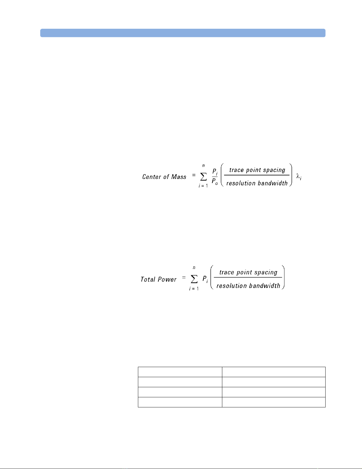
CALCulate Subsystem Commands Programming Commands

CALCulate[1|2|3|4|5|6]:CENTermass:STATe

Turns the Center of Mass (Mean Wavelength) calculation on.

Trace A corresponds to CALCulate1 and so on. Only one Center of Mass calculation may be ON. For instance, if Center of Mass is ON for Trace A, turning Center of Mass ON for Trace B will disable the Center of Mass calculation for Trace A. The data is returned in either ASCII or binary form as determined by the FORMat:DATA command.

The Center of Mass of the trace points is normalized by the ratio of the trace point spacing and the resolution bandwidth. The power and wavelength of each trace point are used to calculate the Center of Mass. The formula used is:

where:

is the wavelength of a single trace point

is the power of a single trace point

is total power as defined below

Total Power

is the summation of the power at each trace point, normalized by the ratio of the trace point spacing and the resolution bandwidth. The formula used is:

where:

is the power of a single trace point

Syntax

CALC:CENT:STAT OFF|ON|0|1

Example

OUTPUT @Osa;"calc1:cent:state on" ! turn center of mass calculation on for trace a

OUTPUT @Osa;"calc1:cent:data?" ! query for center of mass calculation results

ENTER @Osa;Data ! place center of mass data into variable

PRINT Data ! print Center of Mass value

Agilent 86140B Optical Spectrum Analyzer, Second Edition 95

Page 96

Programming Commands CALCulate Subsystem Commands

FWHM 2,355

CALCulate[1|2|3|4|5|6]:FWHM[:DATA]?

Returns the FWHM calculation results in meters.

Trace A corresponds to CALCulate 1 and so on. Corrections to all calculations are made for the slope and variation of the resolution bandwidth filter over the wavelength range of the trace. When CALCulate[1|2|3|4|5|6]:TPOWer:IRANge is on, the calculation is performed over the upper and lower range limits. All calculations (SOURce, CENTermass, FWHM, SIGMa, and TPOWer) share the same line marker limits. Sending this query when the CALCulate[1|2|3|4|5|6]:FWHM:STATe is off will generate an error.

Syntax

CALC:FWHM: [DATA]?

Example

OUTPUT @OSA;”calc1:fwhm:state on” ! turn full width half max on for trace a

OUTPUT @OSA;”calc1:fwhm:data?” ! query for fwhm calculation results

ENTER @OSA; Data ! place fwhm data into variable

PRINT Data ! print Full Width Half Max value

CALCulate[1|2|3|4|5|6]:FWHM:STATe

Turns the Full Width Half Maximum (FWHM) calculation on.

Trace A corresponds to CALCulate 1 and so on. Only one of each calculation may be on. For instance if FWHM is on for Trace A, turning FWHM on for Trace B will disable the FWHM calculation for Trace A. The data is returned in either ASCII or binary form as determined by the FORMat:DATA command.

FWHM (Full Width at Half Maximum) describes the spectral width of the

half-power (-3 dB) points of the trace, assuming a continuous, Gaussian power distribution. The half-power points are those where the power spectral density is one-half that of the peak amplitude. The formula used is:

96 Agilent 86140B Optical Spectrum Analyzer, Second Edition

σ=

where: is sigma as defined in CALCulate[1|2|3|4|5|6]:SIGMa

Page 97

CALCulate Subsystem Commands Programming Commands

Syntax

CALC:FWHM:STAT OFF|ON|0|1

Example

OUTPUT @OSA;”calc1:fwhm:state on” ! turn full width half max on for trace a

OUTPUT @OSA;”calc1:fwhm:data?” ! query for fwhm calculation results

ENTER @OSA; Data ! place fwhm data into variable

PRINT Data ! print Full Width Half Max value

CALCulate:MARKer:AOFF

This command is not available for the filter mode application in the Agilent 86144B/86146B, because this command turns off all markers, including filter mode tune marker.

NOTE

Turns off all markers and marker functions.

Going to zero span will turn off all markers. This is because markers are referenced to a particular time or wavelength not a particular display position. Going out of zero span will restore the markers to the state they were in before going to zero span. Changing to or from zero span changes the fundamental units for the X-axis.

If no marker number is given in the following marker commands, the command is interpreted as referring to marker number 1. For example, CALC:MARK ON is equivalent to CALC:MARK1 ON.

Syntax

CALC:MARK:AOFF

Example

OUTPUT @Osa;"calc:mark:aoff" ! all markers turned off

Related Keys

ACTIVE MARKER 1|2|3|4|OFF

Agilent 86140B Optical Spectrum Analyzer, Second Edition 97

Page 98

Programming Commands CALCulate Subsystem Commands

CALCulate:MARKer[1|2|3|4]:FUNCtion:BWIDth|BANDwidth :INTerpolate

Turns the bandwidth marker interpolation on or off.

When interpolation is on, the bandwidth markers will be placed at the exact number of dB (NDB) setting from the normal marker if the trace data allows. The position of the marker will be linearly interpolated between two true trace data points. The default state is on. If interpolate is off, for negative NDB values, the bandwidth markers will be at values closest to and more negative than the NDB value. For positive NDB values, the bandwidth markers will be at values closest to and more positive than the NDB values. This will typically result in a wider bandwidth measurement.

This is a global setting and controls the interpolation state for all four bandwidth markers.

The query response indicates whether interpolation is turned on or off.

Syntax

CALC:MARK[1|2|3|4]:FUNC:BWID|BAND:INT OFF|ON|0|1

CALC:MARK[1|2|3|4]:FUNC:BWID|BAND:INT?

Example

OUTPUT @Osa;"calc:mark1:func:band:stat on" ! turn bandwidth marker 1 on trace a

OUTPUT @Osa;"calc:mark1:func:band:int on" ! turn bandwidth interpolation on

Related Key

(MARKER SETUP) BANDWIDTH INTERPOLATION ON|OFF

98 Agilent 86140B Optical Spectrum Analyzer, Second Edition

Page 99

CALCulate Subsystem Commands Programming Commands

CALCulate:MARKer[1|2|3|4]:FUNCtion:BWIDth|BANDwidth:NDB

Sets the desired vertical offset from the numbered marker of the bandwidth markers.The parameter units are as specified in the UNIT:RATio command.

This value can be set or queried anytime. The marker does not have to be on or in the bandwidth function.

Syntax

CALC:MARK[1|2|3|4]:FUNC:BWID|BAND:NDB <numeric_value>

CALC:MARK[1|2|3|4]:FUNC:BWID|BAND:NDB?

Example

OUTPUT @Osa;"calc:mark1:func:band:stat on"

OUTPUT @Osa;"calc:mark1:func:band:ndb 3db"

! turn bandwidth marker 1 on trace a

! set the vertical offset of the bandwidth markers

Related Key

(MARKER BW ON OFF) -0.5 DB | -3 DB | -6 DB | -10 DB | -20 DB

CALCulate:MARKer[1|2|3|4]:FUNCtion:BWIDth|BANDwidth:READout

Sets the X-axis readout for frequency or wavelength when the instrument is in a non-zero span.

This setting controls only the bandwidth marker X-axis readouts and the X:Left? and X:Right? queries. The delta markers have their own setting. This setting controls all four bandwidth markers.

Trying to set the readout to TIME when in a non-zero span generates a “Settings conflict” error. Trying to set the readout to FREQuency or WAVelength when in zero span also generates a “Settings conflict” error. When the instrument is set to zero span, the readout will automatically change to TIME. This command is primarily useful for non-zero spans.

Syntax

CALC:MARK[1|2|3|4]:FUNC:BWID|BAND:READ FREQ

Agilent 86140B Optical Spectrum Analyzer, Second Edition 99

Page 100

Programming Commands CALCulate Subsystem Commands

|WAV|TIME

:CALC:MARK[1|2|3|4]:FUNC:BWID|BAND:READ?

Example

OUTPUT @Osa;"calc:mark1:func:band:stat on"

OUTPUT @Osa;"calc:mark1:func:band:read FREQ"

! turn bandwidth marker 1 on trace a

! sets bandwidth marker x query values to !FREQuency

Related Key

(MARKER SETUP) BW MARKER UNITS

CALCulate:MARKer[1|2|3|4]:FUNCtion:BWIDth|BANDwidth:RESult?

Returns the difference in the X-axis values between the left and right bandwidth markers. The units returned are determined by the CALCulate:MARKer:FUNCtion:BWIDth|BANDwidth:X:READout state.

This query generates a “Settings conflict” error if the bandwidth function is

OFF for the specified marker.

For READout of FREQuency, the result is returned in Hertz. For READout of WAVelength, the result is returned in meters. If the bandwidth markers cannot find the desired number of dB (NDB) setting relative to the normal marker, the result returned will be 9.91e37. This value is defined by the SCPI standard to represent NaN (not a number).

Syntax

CALC:MARK[1|2|3|4]:FUNC:BWID|BAND:RES?

Example

OUTPUT @Osa;"calc:mark1:func:band:stat on"

OUTPUT @Osa;"calc:mark1:max" ! set bandwidth marker to strongest signal

OUTPUT @Osa;"calc:mark1:func:bwid:res?" ! query the difference in X values between

ENTER @Osa;Res !left and right bandwidth markers

PRINT Res

! turn bandwidth marker 1 on trace a

100 Agilent 86140B Optical Spectrum Analyzer, Second Edition

Agilent 0B Series Programming Datasheet

Agilent 86140B Series Optical Spectrum Analyzer

Warnings and Notices

Agilent Technologies Sales and Service Offices

Table of Contents

Remote Operation

General Safety Considerations

Safety Symbols

Summary for Experienced GPIB Programmers

Working with Older OSA Applications

Introduction to Controlling an OSA

SCPI Syntax Rules

Monitoring the Instrument

Amplitude Correction Remote Commands

Techniques to Improve Throughput

Sending Remote Commands over the LAN

SICL LAN Set-up Information

Setting Up Your Analyzer as a SICL LAN Server

Setting Up Your Controller as a SICL LAN Client

Example Programs

Example 1. Initialization and a simple measurement

Example 2. Locating the largest signal

Example 3. Bandwidth

Example 4. Maximum and minimum amplitude values

Example 5. Maximum and minimum values over time

Example 6. Returning trace data

Example 7. Trace normalization

Example 8. Total power measurement

Example 9. Monitoring the status registers

Example 10 SMSR calculation with display off

Front Panel Functions to Remote Commands

Programming Commands

Introduction

Command Conventions

Command Trees

Common Commands

*CLS (Clear Status)

*ESE (Event Status Enable)

*ESR? (Event Status Register)

*IDN? (Identification Number)

*OPC (Operation Complete)

*OPT? (Option)

*RCL (Recall)

*RST (Reset)

*SAV (Save)

*SRE (Service Request Enable)

*STB? (Status Byte)

*TST? (Test)

*WAI (Wait-to-Continue)

CALCulate Subsystem Commands

CALCulate[1|2|3|4|5|6]:AVERage:CLEar

CALCulate[1|2|3|4|5|6]:AVERage:COUnt

CALCulate[1|2|3|4|5|6]:CENTermass:[DATA]?

CALCulate[1|2|3|4|5|6]:FWHM[:DATA]?

CALCulate[1|2|3|4|5|6]:FWHM:STATe

CALCulate:MARKer:AOFF

CALCulate:MARKer[1|2|3|4]:FUNCtion:BWIDth|BANDwidth :INTerpolate

CALCulate:MARKer[1|2|3|4]:FUNCtion:BWIDth|BANDwidth:NDB

CALCulate:MARKer[1|2|3|4]:FUNCtion:BWIDth|BANDwidth:READout

CALCulate:MARKer[1|2|3|4]:FUNCtion:BWIDth|BANDwidth:RESult?