

Xovis PC Series, PC2, PC3 User Manual
PC-Series
User manual
Copyright reminder
Copyright © 2016 by Xovis AG, Switzerland.
All rights reserved. No part of this publication may be reproduced, stored in a retrieval
system, or transmitted, in any form by any means, electronic, mechanical, photocopying,
recording, or otherwise, without the prior written permission of the publisher. Printed and
published in Switzerland.
While Xovis AG believes the information included in this publication is correct as of the date
of publication, it is subject to change without notice.
All cited trademarks and registered trademarks are the property of their respective owners.
Non-disclosure reminder
All information in this document is strictly confidential and may only be published by Xovis
AG, Switzerland.
Document history
Version
Date
Author
Comment
1.0
17.11.2014
CG / FLM
First Release
1.1
27.03.2015
CG
Updates for SW release 2.2
1.2
16.04.2015
CG
Updates for SW release 2.2.1
1.3
30.06.2015
CG
Updates for SW release 2.3.1
1.4
22.07.2015
CG / FLM
Mounting instructions now described
in separate document
1.5
29.09.2015
CG / FLM
Updates for SW release 3.0.1
1.6
30.10.2015
CG / FLM
Updates for SW release 3.1.0
1.7
23.12.2015
CG
Updates for SW release 3.2.0
1.8
12.06.2016
CG
Updates for SW release 3.3.0
1.9
22.12.2016
CG
Updates SW release 3.4.0
Table of contents
1 Overview ................................................................................................... 5
Content Declaration ...............................................................................................5
PC-Series hardware concept ..................................................................................5
PC-Series 3D sensor ................................................................................................5
2 Installation Fundamentals ......................................................................... 6
Network requirements ...........................................................................................6
Power over Ethernet ...............................................................................................6
Sensor LED ..............................................................................................................6
3 Configuration & Usage ............................................................................. 7
Person tracking .......................................................................................................7
3.1.1 Person generation ........................................................................................................ 7
3.1.2 Person position / coordinate mode ............................................................................. 8
Setting up a sensor .................................................................................................9
3.2.1 Introduction ................................................................................................................. 9
3.2.2 Setting up the sensor in the network .......................................................................... 9
3.2.3 Xovis Sensor Explorer ................................................................................................. 10
3.2.4 Access the web interface ........................................................................................... 14
3.2.5 Login to the sensor .................................................................................................... 15
3.2.6 Navigation .................................................................................................................. 15
3.2.7 Setup Wizard .............................................................................................................. 17
3.2.8 Live View .................................................................................................................... 42
3.2.9 Analytics View ............................................................................................................ 48
3.2.10 Config View ................................................................................................................ 57
3.2.11 Status View ................................................................................................................. 82
3.2.12 Firmware upgrade ...................................................................................................... 84
3.2.13 Extended analytics ..................................................................................................... 86
3.2.14 Configuration changes from another client ............................................................... 87
3.2.15 Connection warning ................................................................................................... 88
4 Troubleshooting ...................................................................................... 89
False behavior ....................................................................................................... 89
Masks .................................................................................................................... 89
4.2.1 Exclusion masks ......................................................................................................... 89
4.2.2 Taboo masks .............................................................................................................. 90
4.2.3 Example for mask differentiation ............................................................................... 92
Placement of dwell zones ..................................................................................... 93
Time synchronization mechanism ....................................................................... 95
5 Technical data ......................................................................................... 97
6 Certificates / Tests ................................................................................... 98
7 Custom Integration ................................................................................. 99
API ......................................................................................................................... 99
Plugin Architecture ............................................................................................... 99
5 / 99 www.xovis.com
1 Overview
Content Declaration
This manual is intended for administrators and users of the PC-Series sensor and is
applicable for software version 3.3.0 and later. It includes instructions for installing, using
and managing the sensor on your network. Basic knowledge of network configuration and
knowledge of the specific network in which the sensor is operated are required when using
this product. Later versions of this document will be published in the customer section on
the Xovis website at www.xovis.com.
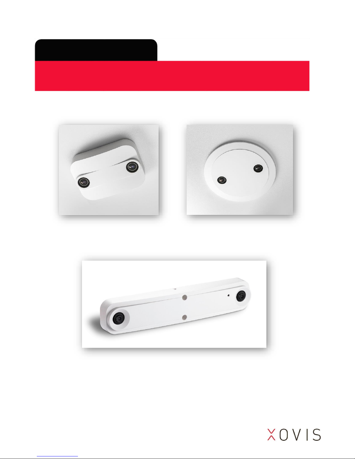
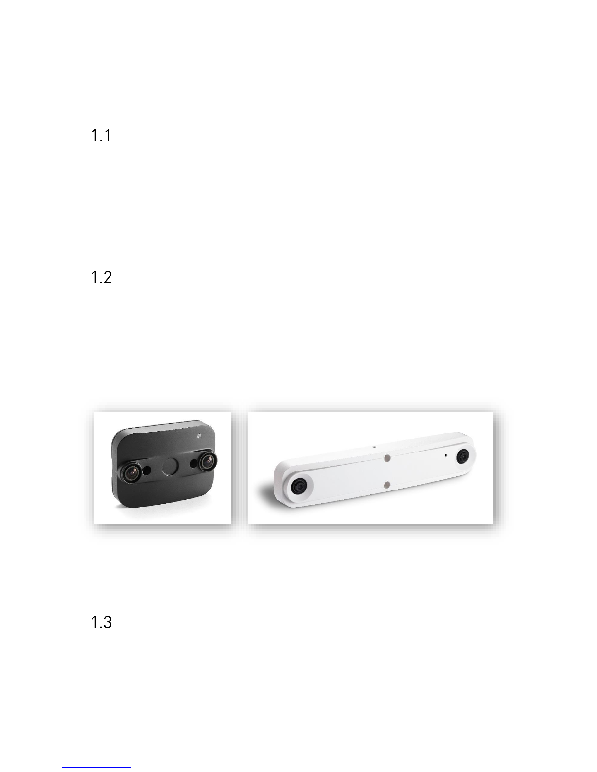
PC-Series hardware concept
The housing of a PC-Series sensor is designed to be mounted directly on the ceiling. Xovis
offers several accessories allowing different installation alternatives. Please refer to the
accessory overview and the mounting instruction showing all versions.
The housing has two holes for sensor positioning and fixation. The Ethernet connector is on
the backside.
Figure 1: PC2 (left) and PC3 (right) 3D sensor
PC-Series 3D sensor
The PC2 3D sensor comes in a black metal housing and supports ceiling heights up to 6.0m.
The PC3 3D sensor comes in a white metal housing and supports ceiling heights up to 20m.
6 / 99 www.xovis.com
2 Installation Fundamentals
Network requirements
The device needs to be connected to the network by a shielded Cat 5 RJ45 Cable. The plug
and the sensor need to be free from any mechanical pressure. The sensor supports Ethernet
10/100Mb Full/Half/Auto negotiation based on the IEEE 802.3 standard. It is highly
recommended to set the switch port to auto negotiation.
Power over Ethernet
The sensor is powered by PoE Class 0 compliant to IEEE 802.3af. As defined by the standard,
the network switch port needs to provide 15 Watts at 48 V.
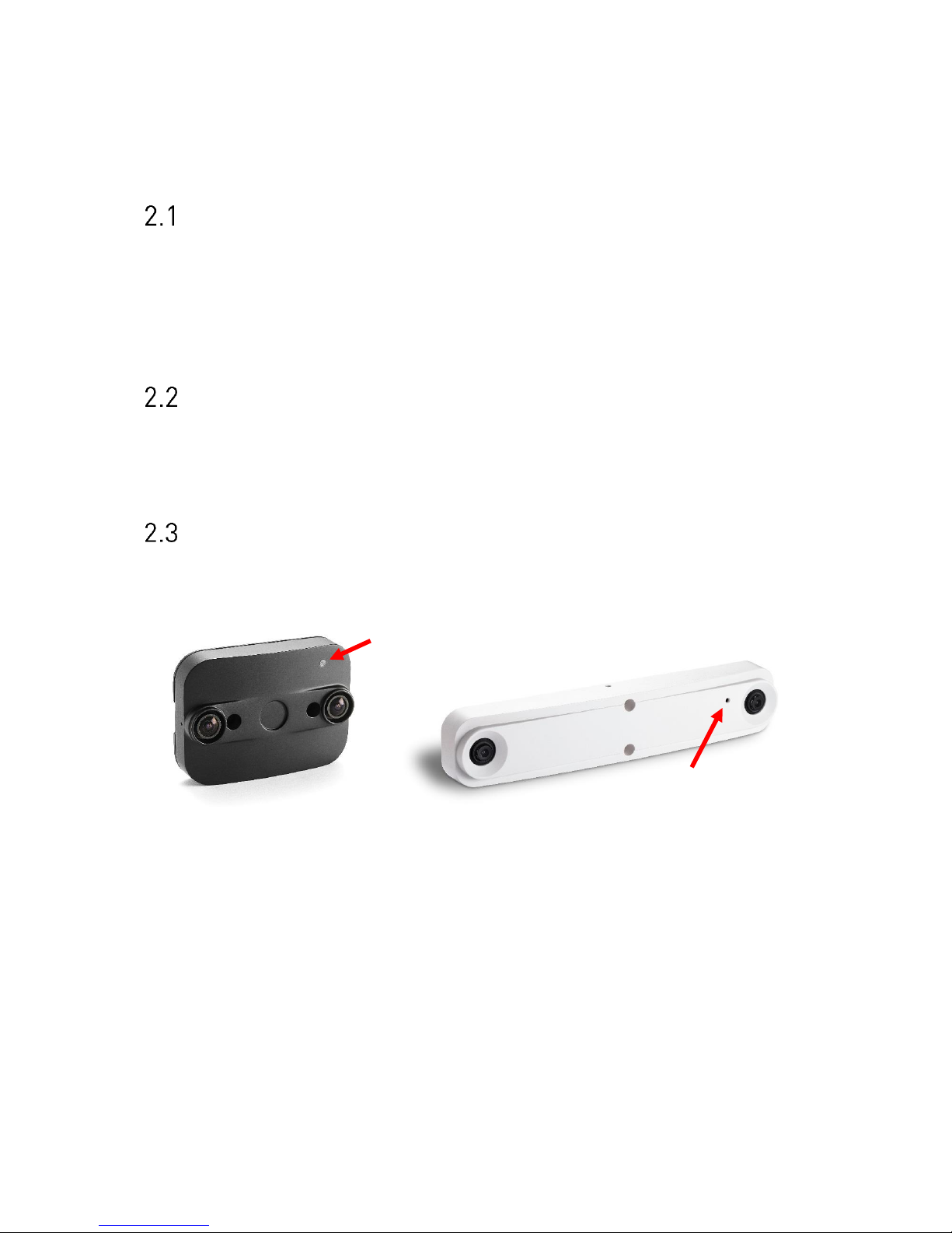
Sensor LED
The PC-Series sensor provides a multifunctional LED on the front side. The red arrow on the
next picture indicate the LED on the PC2 and PC3 models.
Figure 2: PC2 LED (left) and PC3 LED (right)
The LED indicates the following states:
- Green: Device is powered by PoE
- Orange/Green blinking: Device is up and running
The LED state can be useful during installation. When using the optional housing, the LED
will be covered after successful mounting.
7 / 99 www.xovis.com
3 Configuration & Usage
Person tracking
The Xovis PC-Series sensor tracks persons. A few things have to be taken into account to
understand how the detection and tracking of persons works:
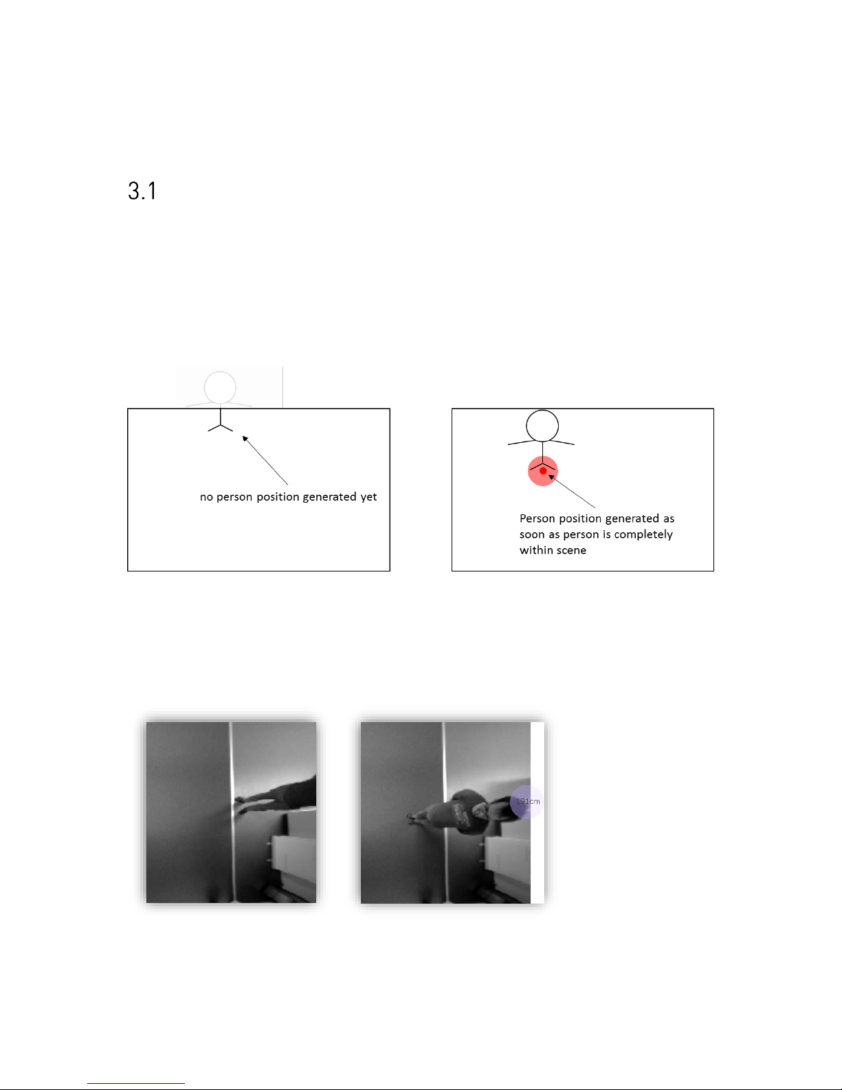
3.1.1 Person generation
The PC-Series sensor generates a person first when the person is completely within the
visible scene (see Figure 3).
Figure 3: Person generation
When a person track once was generated, the person stays tracked until it leaves the scene
again and its head is touching the visible scene border. Tracking/counting at border is
therefore not supported for persons only partially within the scene.
The following situation illustrates the person generation capability:
Figure 4: Demonstration of person generation with coordinate mode “head”
The situation shows that a person is first detected by the sensor when its head is completely
visible i.e. within the scene.
8 / 99 www.xovis.com
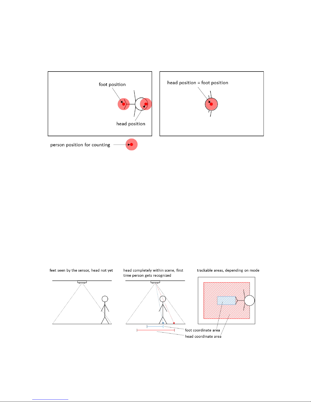
3.1.2 Person position / coordinate mode
The PC-Series sensor uses one specific position per person to evaluate the counting on lines
and zones. This position is either located at the head of a person or at its feet. Figure 5
illustrates the two possible positions.
Figure 5: Person position
Due to the visual perspective of the overhead mounted sensor, the head and foot positions
are congruent directly underneath (in the plump) of the sensor but at different positions at
the scene borders. The user can choose which position shall be used on the sensor by
defining the coordinate mode. This coordinate mode, which can either be “foot” or “head”,
then defines where to show the tracking of a person.
The displaying of the person tracks (paths) on the other hand influences the definition of the
counting elements: When choosing foot coordinates, the person paths will first be displayed
after an offset from the border, as persons get detected by the sensor first, when their head
is seen by the sensor. And, due to the visual perspective, the feet of a person will be seen by
the sensor long before the head of the same person is seen. Or, in other words, when a
persons head is seen by the sensor, its feet will be located within the sceen with a certain
distance to the border / to the head of the person. The following situation demonstrates this
fact:
Figure 6: Different tracking areas depending on the coordinate mode
9 / 99 www.xovis.com
Theoretically the foot coordinates will always be the easier way to use, as all counting items
(e.g. count line) can then just be oriented on the scenes floor (all possible locations of a
persons feet are given by considering the floor of the scene). But due to the visual
perspecitive, feet positions will not be displayed within the complete visible floor which can
complicate the proper drawing of counting items, especially on lower mounting heights
where the difference between the trackable areas of both coordinate modes is quite big (see
Figure 6). Therefore, in some situations, head coordinates can be the preferred choice.
The following situation illustrates the two different coordinate positions:
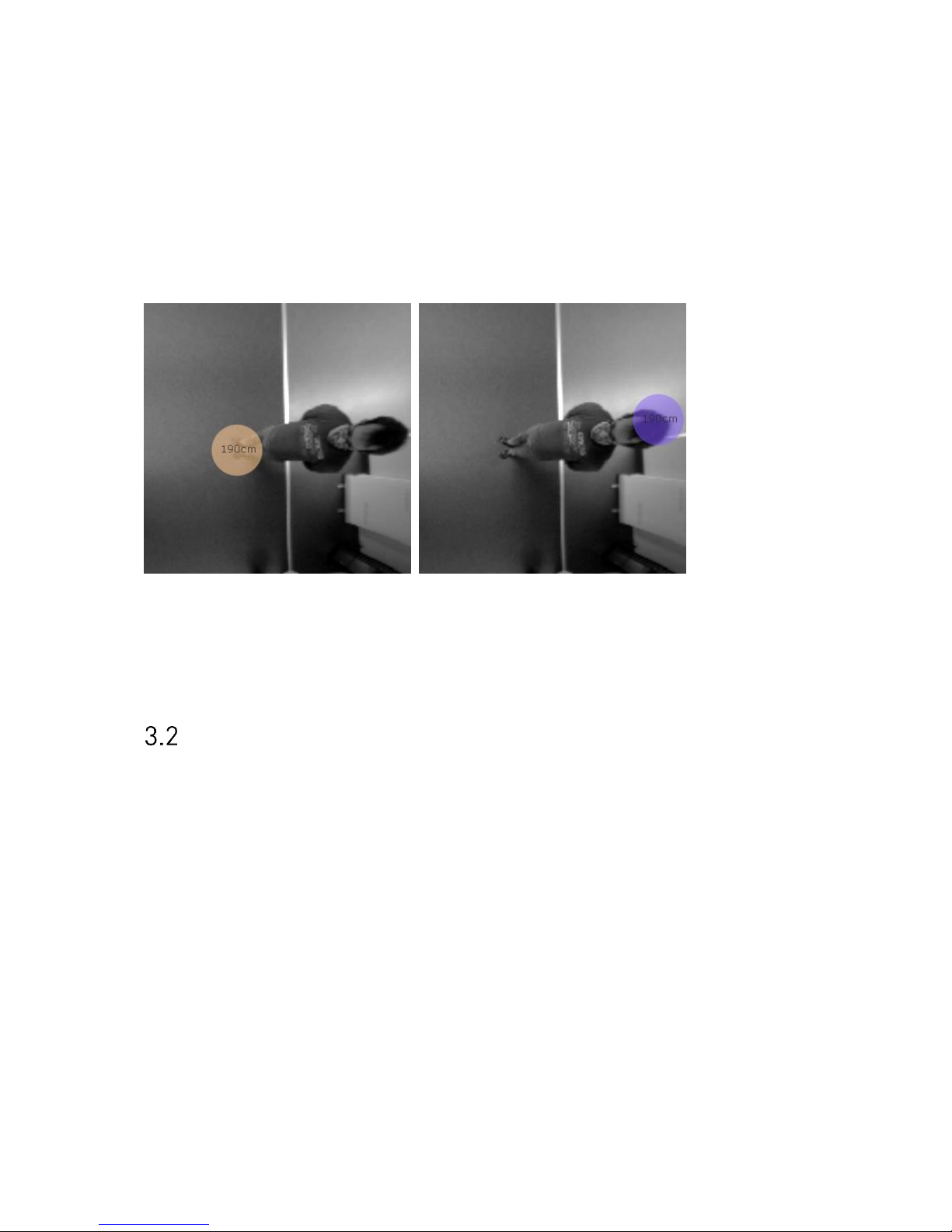
Figure 7: Demonstration of coordinate modes
In the left image, foot coordinates are in use. In the right image, head coordinates are in use.
The situation shows that the first possible position of person “bubbles” is clearly closer at
the border when using head positions.
Setting up a sensor
3.2.1 Introduction
This chapter describes the recommended procedure how to set up a new PC-Series sensor.
3.2.2 Setting up the sensor in the network
The sensor is setup for use in a DHCP environment by default. If a sensor is attached to a
network, it is expecting an IP address assignment by a DHCP server in the network. This is
the simplest way to install a new sensor.
If no DHCP server is present, a static IP setting needs to be applied to the sensor. For this
purpose, a Windows PC attached to the same physical subnet as the sensor is required. The
static network settings can then be applied with the Xovis Sensor Explorer tool, which is
described in the next chapter.
10 / 99 www.xovis.com
3.2.3 Xovis Sensor Explorer
The Xovis Sensor Explorer tool offers a simple way to install and manage Xovis sensors in the
network.
3.2.3.1 Discover sensor on the network
The Xovis Sensor Explorer can be run without installation directly by double-clicking the
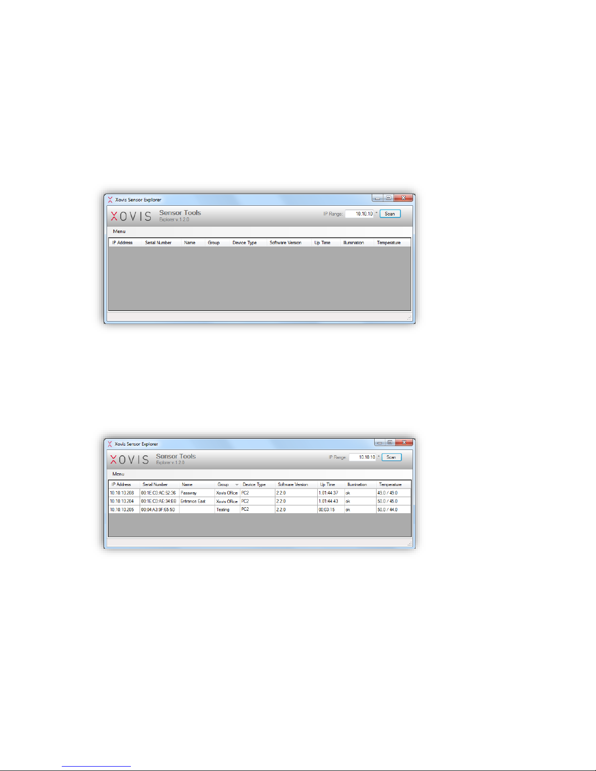
XovisSensorExplorer.exe file. The following screen shows up:
Figure 8: Xovis Sensor Explorer
On the top right of the screen, an IP range can be specified. This range will be scanned for
Xovis sensors when clicking on the “Scan” button. Every sensor properly configured in the
specified IP subnet will be discovered and listed in the Xovis Sensor Explorer. Figure 9
shows an example:
Figure 9: Found sensors on the network
11 / 99 www.xovis.com
For all discovered sensors the Xovis Sensor Explorer will display a series of information
which can be useful for maintaining the Xovis sensors in a network:
Item
Description
IP Address
The sensors IP address
Serial Number
Serial number of the sensor
Name
The sensor name, if set
Group
The sensor group, if set
Device Type
The type of the sensor (e.g. PC2, PC2-UL, PC3)
Software Version
The version of the software currently running on the sensor
Up Time
The sensors uptime in the format d.hh:mm:ss
Illumination
The illumination status of the scene in which the sensor is operating,
can be “ok” or “insufficient”
Temperature
The sensors temperature in degrees Celsius whereby the first number
represents the sensors housing temperature and the second number
the sensors internal temperature
3.2.3.2 Installing a sensor in a fix IP environment
The Xovis Sensor Explorer will only display sensors properly configured and reachable on the
network. In a fix IP environment, a newly attached sensor needs to be setup with a valid IP
configuration first to be able to get discovered by the Xovis Sensor Explorer (the default IP
address of the sensor when no DHCP is in use is 192.168.1.168). For this purpose, the Xovis
Sensor Explorer allows to temporarily apply a specific IP setting to any sensor physically
attached to the same subnet, regardless of whether the sensor was already discovered and
therefore displayed in the Xovis Sensor Explorer list or not, just by specifying the sensors
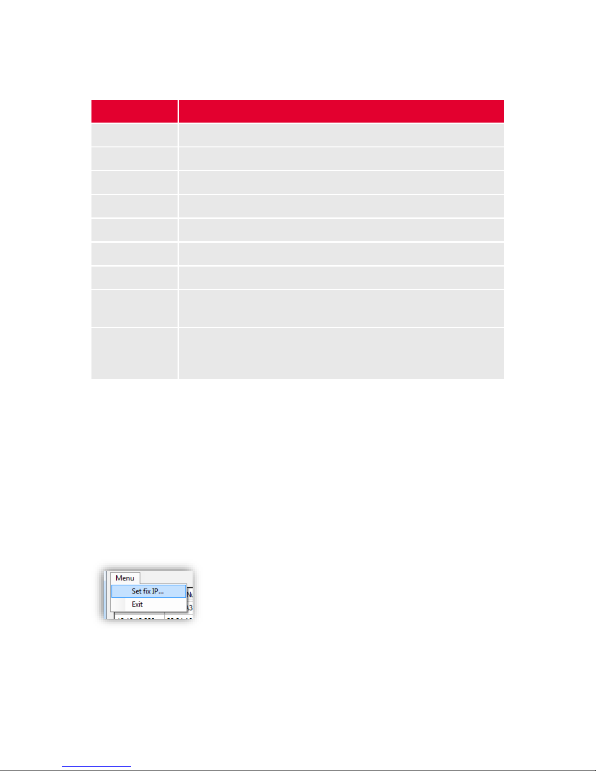
serial number and the desired network configuration. The menu located directly beneath the
Xovis lettering in the top left of the screen contains the menu item “Set fix IP…” (see Figure
10).
Figure 10: Set fix IP menu item
12 / 99 www.xovis.com
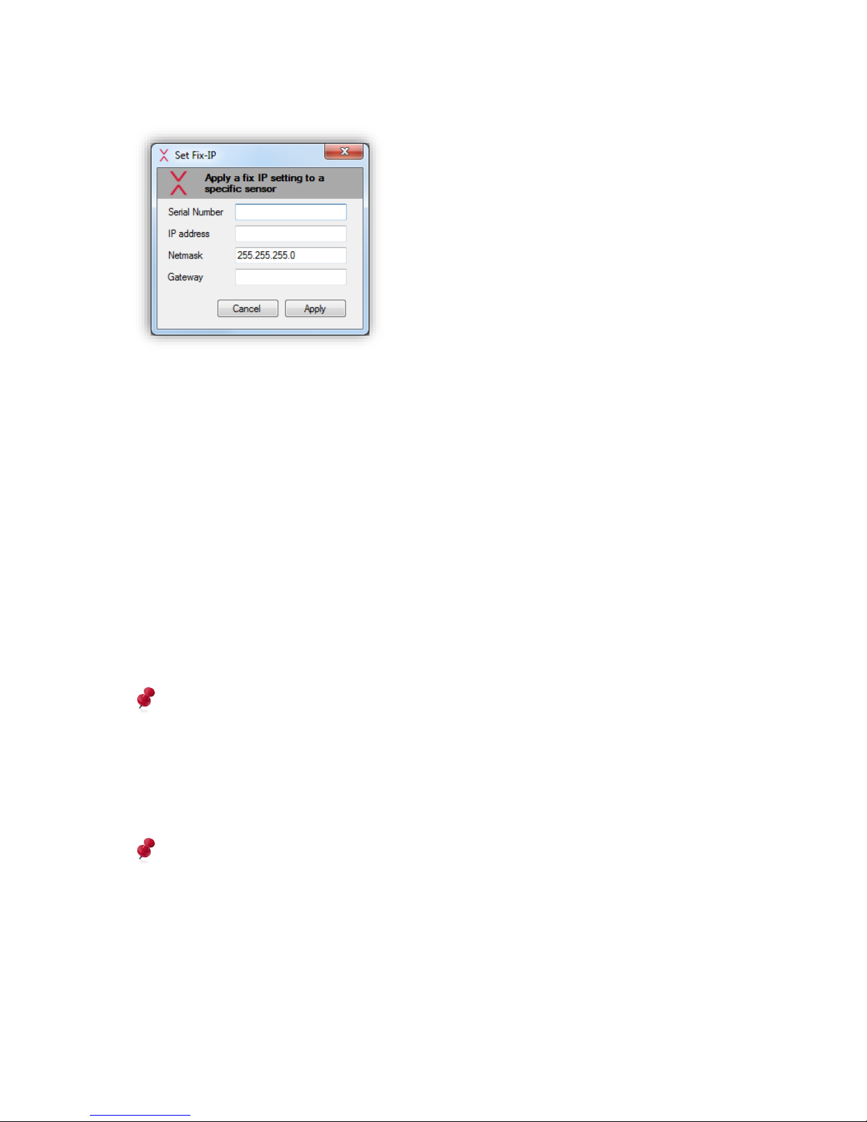
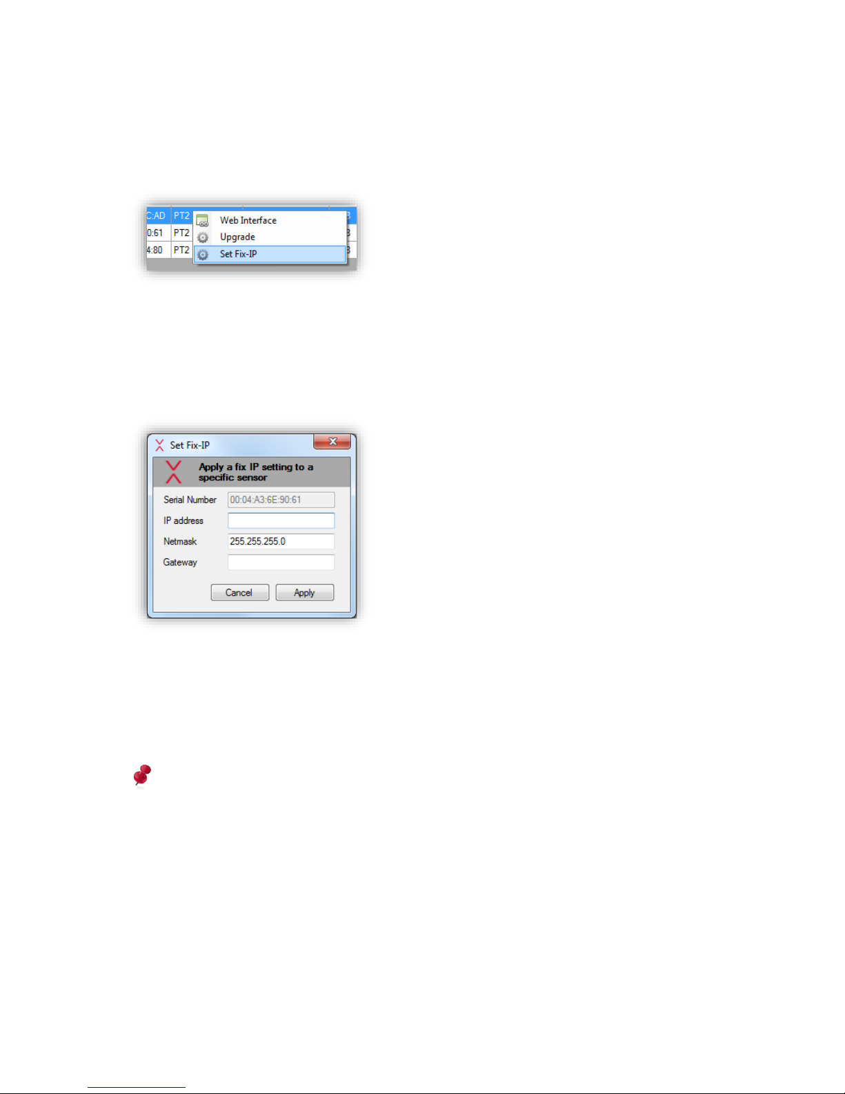
By clicking it, the following dialog appears:
Figure 11: Set Fix-IP dialog
In the first field, the serial number of the sensor needs to be specified. The correctness of
this number is very important and needs to be in the format XX:XX:XX:XX:XX:XX (X to be
replaced). The serial number can be found on the back side of the sensor or on the package
in which the sensor was delivered.
In the fields “IP address”, “Netmask” and “Gateway”, the desired network settings need to be
specified, i.e. the fix IP settings to be applied on this sensor. All fields are required. When
pressing “Apply”, the specified settings are sent to the sensor and a message informs the
user to be patient for 20 seconds. After this time, the sensor should have come up with the
new IP settings.
If the PC running the Xovis Sensor Explorer is located in the same IP range or allows routing
to the IP range of the previously configured sensor, the Xovis Sensor Explorer is now able to
discover the sensor when specifying the proper IP range and clicking again on the “Scan”
button.
The sensor needs to be attached to the same physical subnet as the Windows PC running
the Xovis Sensor Explorer.
As the static IP was only set temporarily and will be lost with the next reboot of the sensor it
is now important to apply the desired IP settings permanently using the web interface (see
following chapters).
After temporarily applying a static IP with this procedure, it is important to permanently
set the fixed IP-address in the web interface afterwards!
13 / 99 www.xovis.com
3.2.3.3 Setting a fix IP address to a discovered sensor
The Fix-IP dialog (see chapter “3.2.3.2 Installing a sensor in a fix IP environment”) can also
be opened for any sensor already discovered by the Xovis Sensor Explorer by simply rightclicking on it in the list and choosing “Set Fix-IP” in the popping up menu (see Figure 12).
Figure 12: Set Fix-IP
The same dialog as described in chapter 3.2.3.2 shows up with the single difference that the
serial number field is already filled with the one of the selected sensor. The remaining fields
again request the user to specify the IP address, the subnet mask and the gateway for the
specific sensor:
Figure 13: Set Fix-IP dialog
After applying the IP settings to the sensor by clicking the “Apply” button, the specified
settings are sent to the sensor and a message informs the user to be patient for 20 seconds.
After this time, the sensor should have come up with the new IP settings and can be found in
the according network and IP range.
After temporarily applying a static IP with this procedure, it is important to permanently
set the fixed IP-address in the web interface afterwards!
3.2.3.4 Upgrading a sensor
A sensors software / firmware can be upgraded by right clicking on a specific sensor in the
list of the Xovis Sensor Explorer and choosing “Upgrade” in the appearing dropdown menu.
In the appearing file dialog, an upgrade file of the type “xfw” (file extension) needs to be
selected. After applying a valid upgrade file, the sensor will instantaneously start with the
upgrade procedure which usually takes about 3 minutes. When refreshing the list of sensors
in the network by clicking again on the “Scan” button of the Xovis Sensor Explorer after these
3 minutes, the upgraded sensor will appear with updated software version.
14 / 99 www.xovis.com
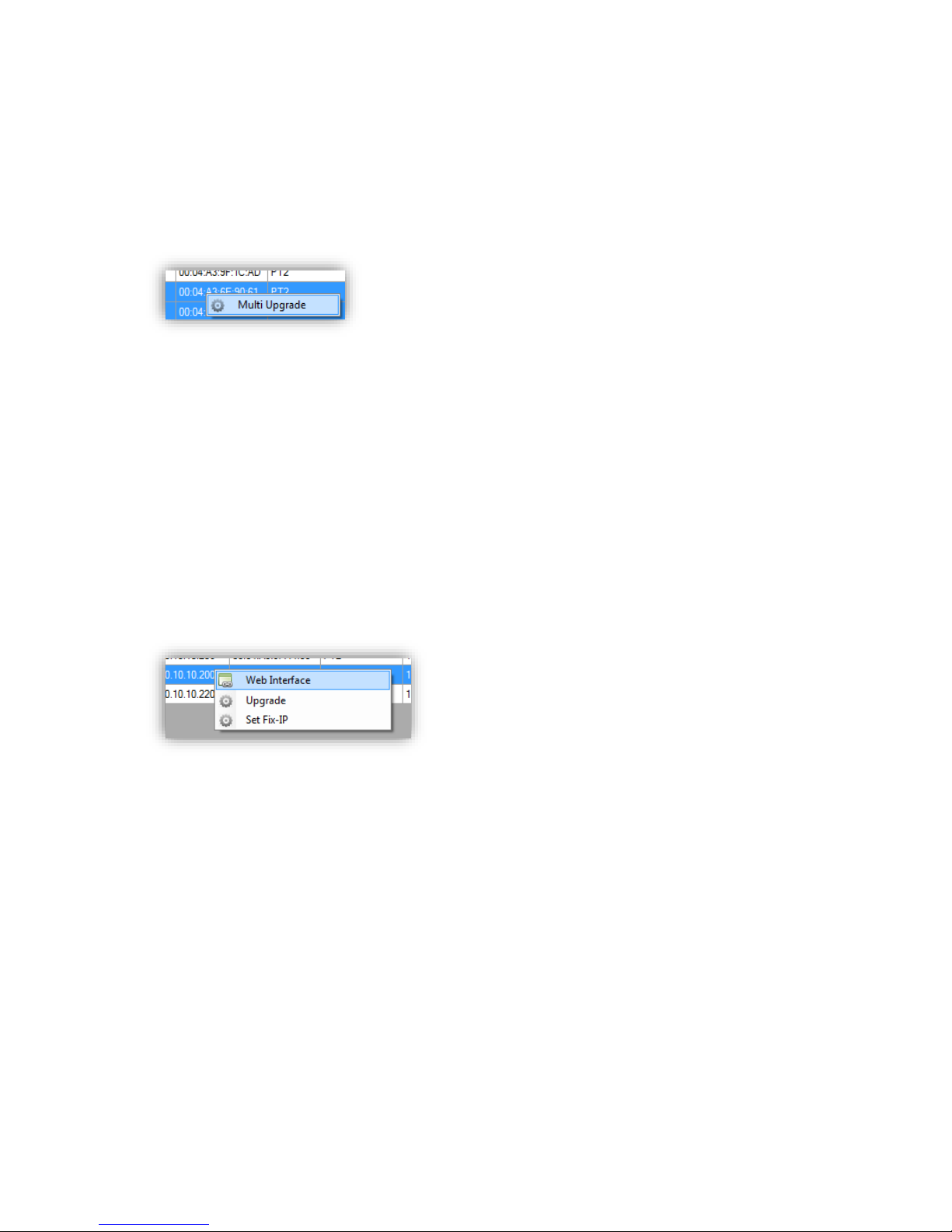
An upgrade can also be applied to multiple sensors at the same time by selecting all or a
part of the sensor in the list of the Xovis Sensor Explorer with [Ctrl] + [A] or pressed [Ctrl]
and left mouse click on the desired sensors. A right click on the selection opens a popup
menu with the only item “Multi Upgrade” (see Figure 14). Clicking it opens the same file
dialog as for upgrading a single sensor but will distribute the chosen upgrade file to all
selected sensors at the same time when applying.
Figure 14: Multi Upgrade
A sensors software / firmware can also be upgraded via its web interface. This procedure is
described in chapter 3.2.12.
3.2.4 Access the web interface
The sensor web interface is accessed by typing its IP address directly into a web browser on
a PC connected to the same network as the sensor. Alternatively, the sensors web page can
be opened by double-clicking a sensor in the Xovis Sensor Explorer or by clicking the menu
item “Web Interface” in the popup menu appearing when right-clicking on a sensor in the
Xovis Sensor Explorer (see Figure 15). The web page will be opened in the default browser of
the operating system.
Figure 15: Menu item “Web Interface” in Xovis Sensor Explorer
3.2.4.1 HTTPS
The sensor web interface can also be accessed over HTTPS by just declaring the protocol
accordingly (https://).
3.2.4.2 Supported browsers
The sensor user interface is an HTML/JavaScript based website. The following web browsers
offer a proper functionality of the website:
- Firefox 4 or newer
- Google Chrome version 10 or newer
- Microsoft Internet Explorer version 10 or newer
- Apple Safari version 5 or newer
- Opera version 12 or newer
15 / 99 www.xovis.com
Recommended browsers are Firefox, Chrome, Opera and Internet Explorer.
For all browsers JavaScript support needs to be enabled and all caching for this website
needs to be switched off!
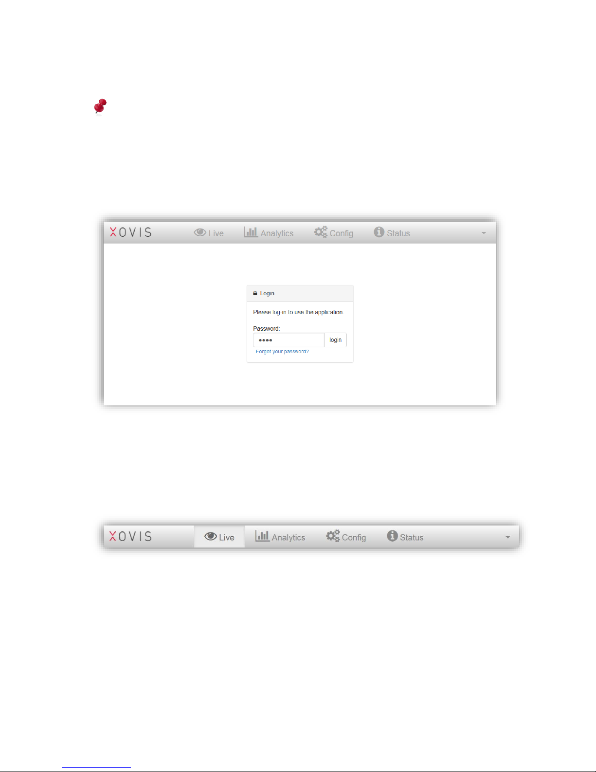
3.2.5 Login to the sensor
The arrival page of the website shows a log-in dialog. The default password is “pass”
(without the “”).
Figure 16: Login screen
The login screen holds a “Forgot your password” link. This allows to reset the sensor using
the Sensor Master Key (SMK). The reset procedure is described in chapter 3.2.10.4.5.
3.2.6 Navigation
The navigation bar is located at the top of the web GUI. It basically holds three sections: The
logo, the menu buttons and a context menu.
The menu buttons allow the user to switch between the four main views “Live”, “Analytics”,
“Config” and “Status”. The purpose of these views is described in their respective chapters
3.2.8 to 3.2.11. These buttons are disabled when logged out and in the setup wizard mode
(see next chapter).
16 / 99 www.xovis.com
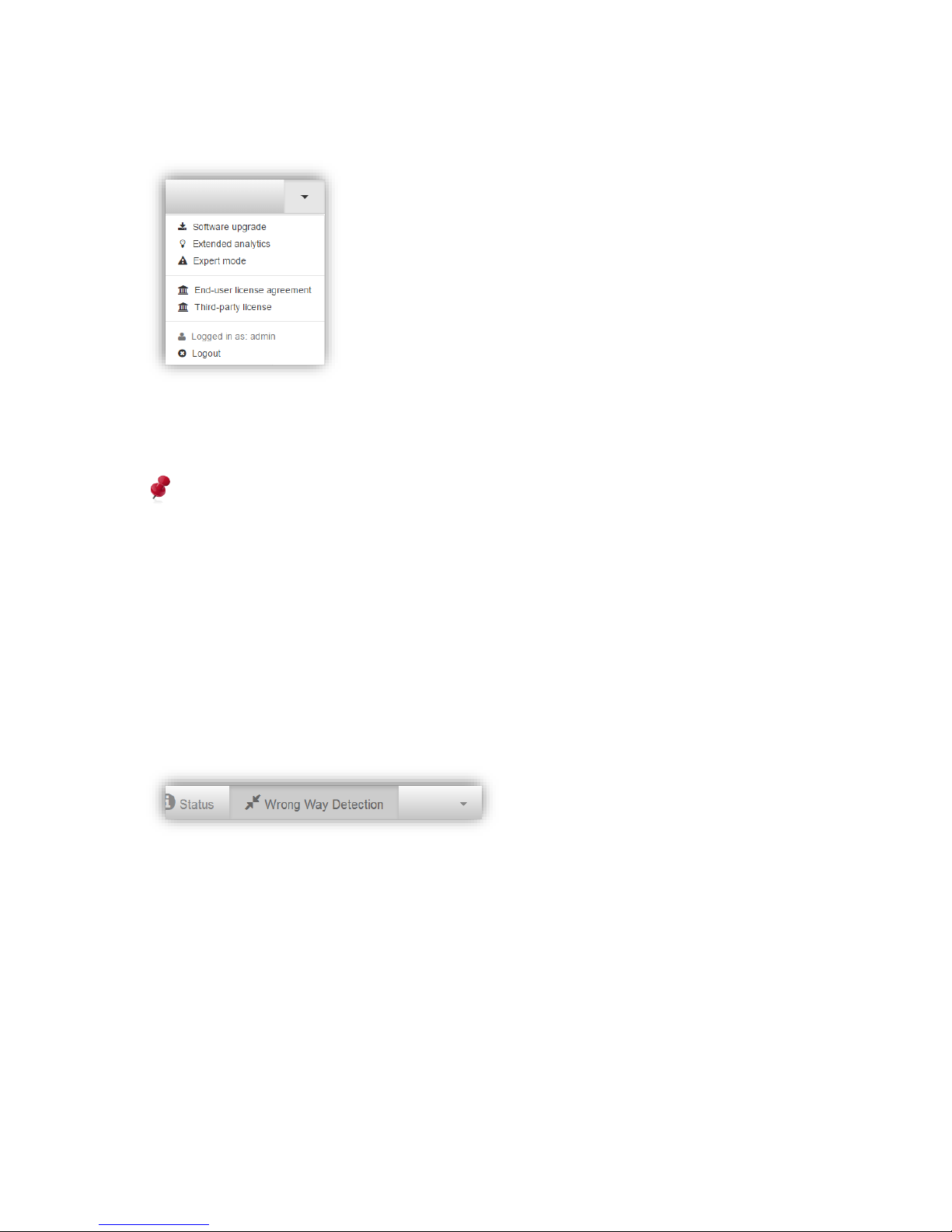
The context menu holds additional functionalities for maintaining the sensor and to logout
the current user:
The “Software Upgrade” procedure will be explained in chapter 3.2.12. “Extended Analytics”
is covered in chapter 3.2.13. The “Expert Mode” is not documented in this manual as it is
reserved for expert use only.
Xovis strongly recommends to NOT USE the expert mode at all as changes made with the
expert mode can cause the sensor to become unresponsive.
The two entries for EULA and third-party licenses display the respective licenses.
The “Logout” button ends the session of the currently logged in user and returns to the login
page. The currently logged in user is displayed directly above the “Logout” button.
3.2.6.1 Plugins
The PC2 sensor can be enriched with various plugins. The plugin installation procedure is
described in chapter 3.2.10.4.3. Plugins which offer a frontend component will also be listed
in the navigation bar. Figure 17 shows an example with the “Wrong Way Detection” plugin:
Figure 17: Plugin button in the navigation bar
A plugins functionality and usage is documented in the documentation of the specific plugin.
17 / 99 www.xovis.com
3.2.7 Setup Wizard
As long as the sensor is not configured, the setup wizard will be shown directly after loggingin.
It is strongly recommended to use the setup wizard for setting up the sensor as the wizard
ensures to gather all information needed for a proper usage of the sensor.
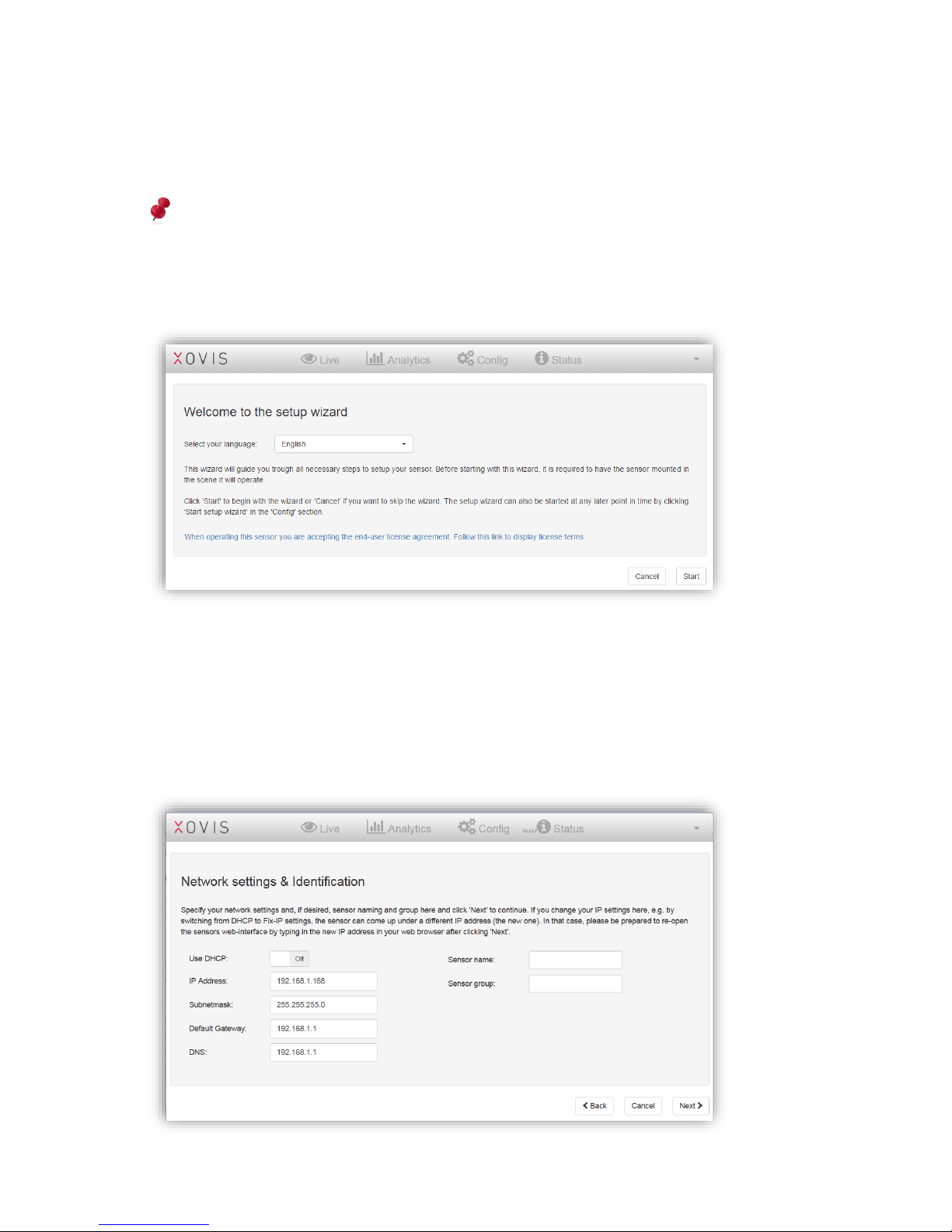
3.2.7.1 Welcome screen
Figure 18: Setup wizard
The welcome screen of the wizard gives a quick description of the intent of the wizard and
allows the user to choose the desired GUI language. The wizard can be started by clicking
“Start”. At any step of the wizard, it can be ended by clicking “Cancel”. The setup wizard can
be re-started anytime in the config view (see chapter 3.2.10.1.3).
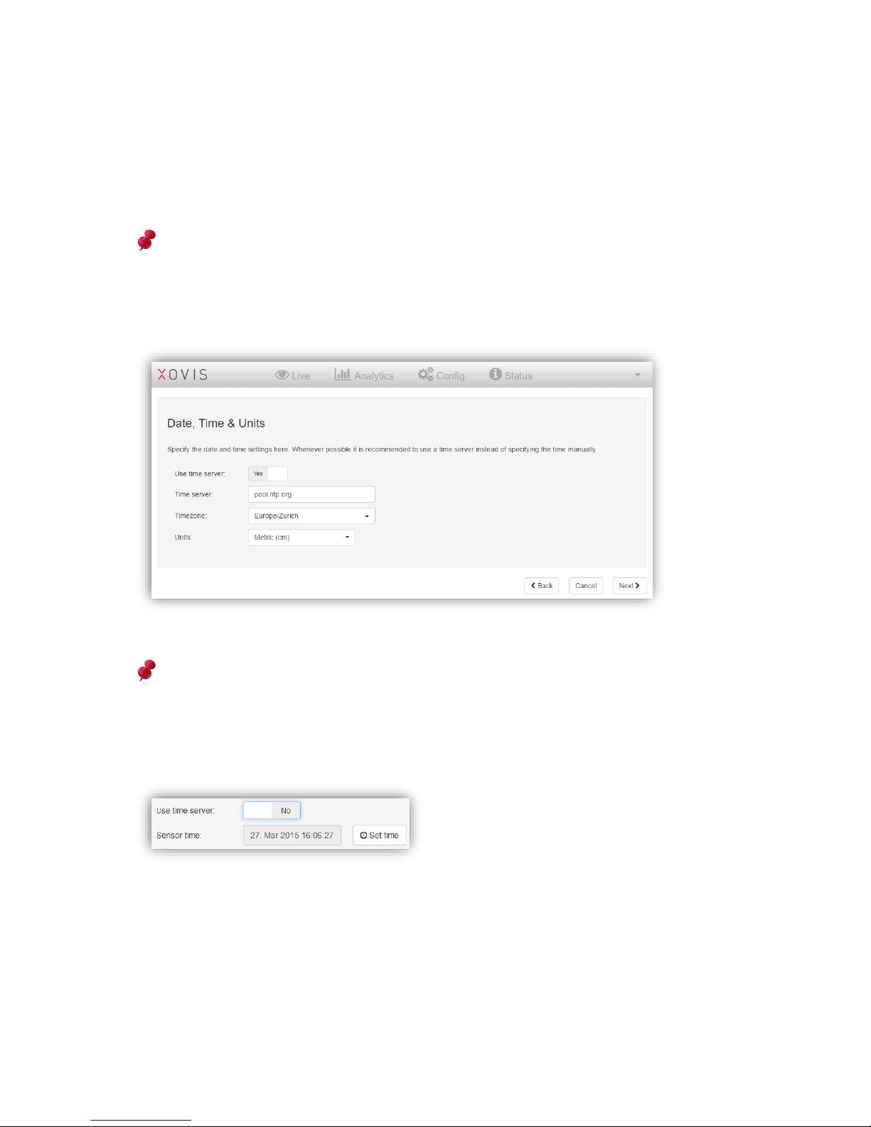
3.2.7.2 Network settings & Identification
18 / 99 www.xovis.com
As first step, the wizard is asking for the network settings and identification naming. The
sensor can be run with DHCP or a fix IP address. If not using DHCP and the IP settings have
been applied already by using the Xovis Sensor Explorer (see chapter 3.2.3.2), it is
recommended to double check the network settings here. Optionally, a name and group can
be specified for the sensor. By clicking “Next”, the network settings are applied to the
sensor.
If the IP address of the sensor is changed here, the sensor will instantaneously come up
under the new address after pressing “Save”. In that case the new IP address needs to be
entered in the web browser after saving.
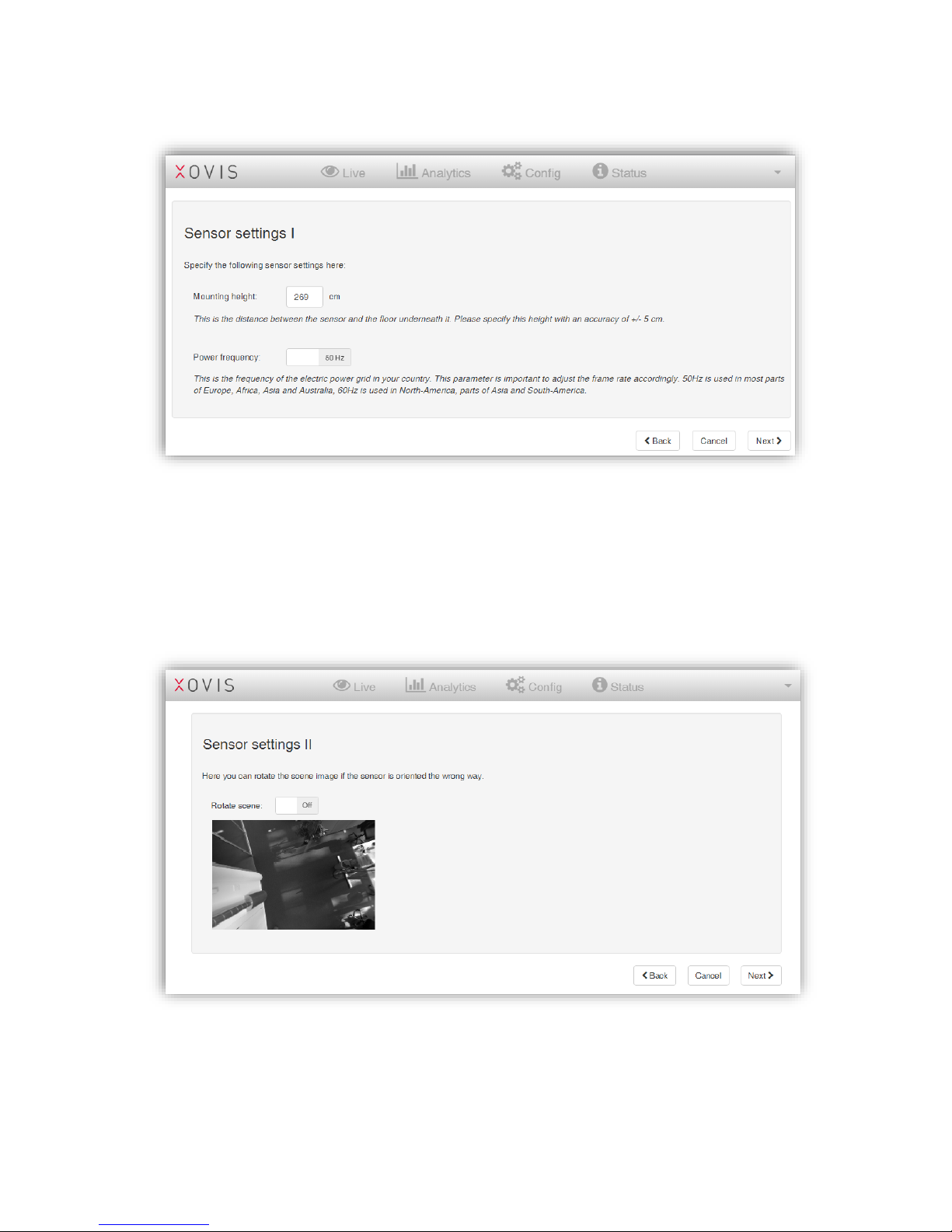
3.2.7.3 Date & Time
In the next screen the wizard is asking for setting the sensors date, time and units.
Whenever possible it is recommended to use a timeserver, as a correct time can be
crucial for stored counting data statistics.
When not using a time server, the sensor time can be set manually by switching the “Use
time server” toggle to “No” and then clicking on “Set time”:
The time zone dropdown is ordered by continents / geographic regions and cities. The time
zone should be set according to the sensors location.
The “Units” dropdown allows to choose between Metric (cm) and Imperial (feet/inch) units.
By clicking “Next”, the date and time settings are applied to the sensor.
19 / 99 www.xovis.com
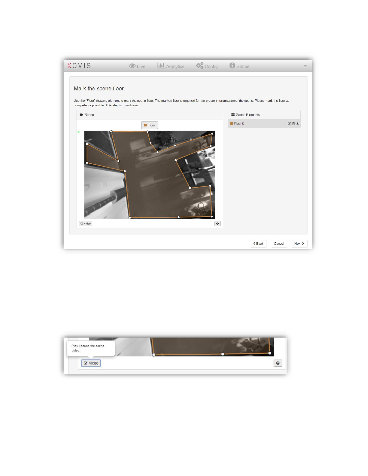
3.2.7.4 Sensor settings I
In the next screen, some base settings for the sensor operation need to be specified. First,
the mounting height needs to be set as accurate as possible. Second, the user is asked to
specify the power frequency of the country of operation. This is needed to adjust the sensors
frame rate to the illumination frequency. By clicking “Next”, these settings are applied to the
sensor.
3.2.7.5 Sensor settings II
In the succeeding screen, the scene image can be rotated by 180 degrees if desired. This can
be of use if the user’s sense of the scene view differs from the orientation of the mounted
sensor. The orientation is applied by clicking “Next”.
20 / 99 www.xovis.com
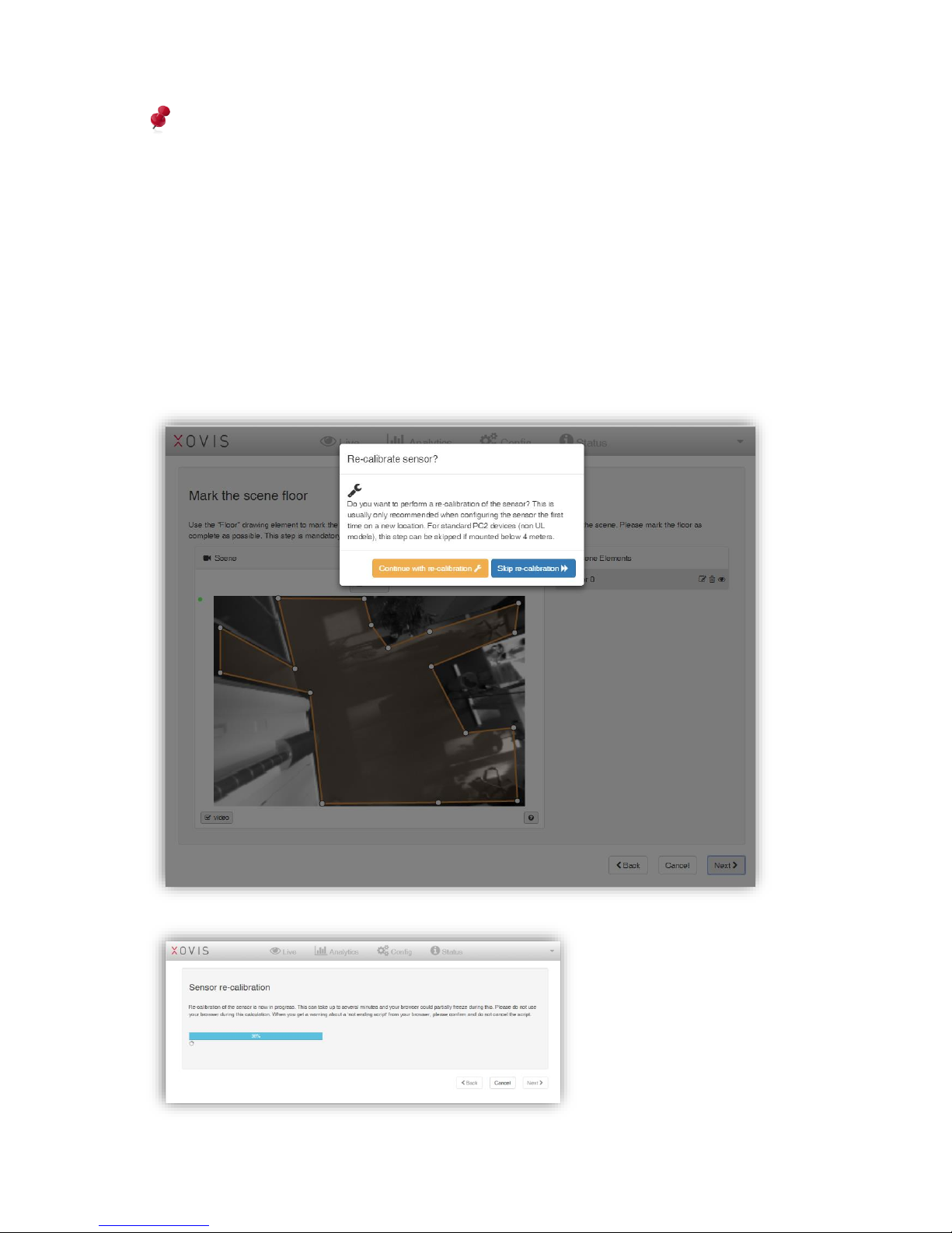
3.2.7.6 Mark the scene floor
Figure 19: Drawn scene floor
In the next screen, the user is asked to mark the scene floor. The displayed scene image by
default is a still image as this usually simplifies the analysis of the scene environment.
However, if a video stream is preferred or maybe to just recapture a new still image, the live
stream can be displayed by clicking on the play button located below the scene image. The
help button beside the play button also offers a short explanation when hovering over it with
the mouse:
The floor is masked by selecting the drawing tool “Floor” and directly drawing the whole
floor as a polygon in the scene (see Figure 19). With the “Floor” tool activated, one can simply
click in the scene image to draw corners of a floor area. A floor area is finished by clicking on
the first corner again, by double-clicking to create the last corner, by disabling the “Floor”
tool or by pressing [Esc] on the keyboard. After finishing a floor area, one is asked to name it
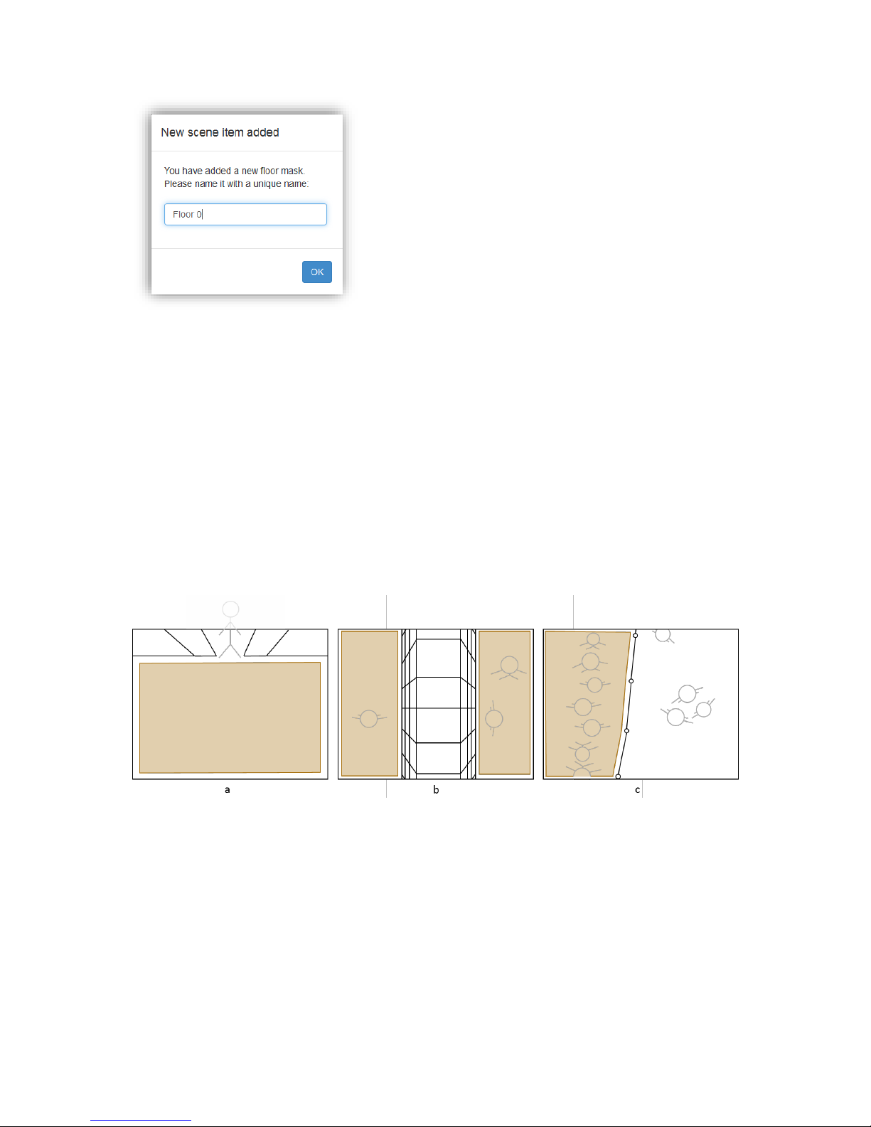
(see Figure 20). A default name is proposed.
21 / 99 www.xovis.com
Figure 20: Name a scene item
As for all scene elements, this name must be unique among all other scene elements like
count lines and count zones. But at this point, the floor item will be the first scene item
added. After specifying a name, the floor is automatically added to the scene element list on
the right. There can also be more than one floor area (element) in the scene, e.g. for two
corridors covered by one sensor or just to simplify the drawing procedure for the user (see
Figure 21 b).
The floor mask defines the area in which persons should be detected by the sensor and
refers to the feet positions of a person. Usually the whole floor contained in a scene should
be covered by the floor mask. For special situations it can be desired to limit the floor mask
to a part of the actual floor only, e.g. when persons passing in a neighboring zone should be
ignored (see Figure 21 c).
Figure 21: Floor mask in different scene situations
As Figure 21 shows, it is a good practice to keep a small distance between the floor mask
and limiting objects like walls, doors or shelves. As mentioned already, it is also possible to
use more than one floor masks if the situation is demanding this.
To modify a floor mask the polygon points can simply be moved with the mouse. Doubleclicking on a polygon point will delete it, double-clicking on the polygon line will add an
additional point to the polygon. The whole polygon can be moved by clicking and holding the
mouse within the floor mask area and moving it to the desired location (drag-and-drop).
22 / 99 www.xovis.com
The wizard requires the user to add at least one floor mask before continuing. However,
after finishing the wizard, the floor mask can theoretically be removed again. In that case,
if no floor mask is used, the whole scene is considered as floor and therefore enabled for
person detection.
The floor mask is applied when clicking “Next”.
3.2.7.7 Re-calibrate Sensor
The wizard will now ask if a re-calibration should be applied. It is recommended to recalibrate the sensor when installing it for the first time in a new location. This step can be
skipped for standard PC2 devices being installed below 4 meters height and not in use in a
multisensor.
23 / 99 www.xovis.com
The recalibration requires a data exchange between the sensor and the web browser. If
performed by remote, the connection bandwidth will impact the duration and can take
several minutes. In such case we suggest a connection with at least 200kbytes/s.
When the re-calibration is done, it is applying to the sensors by clicking on “Next”.
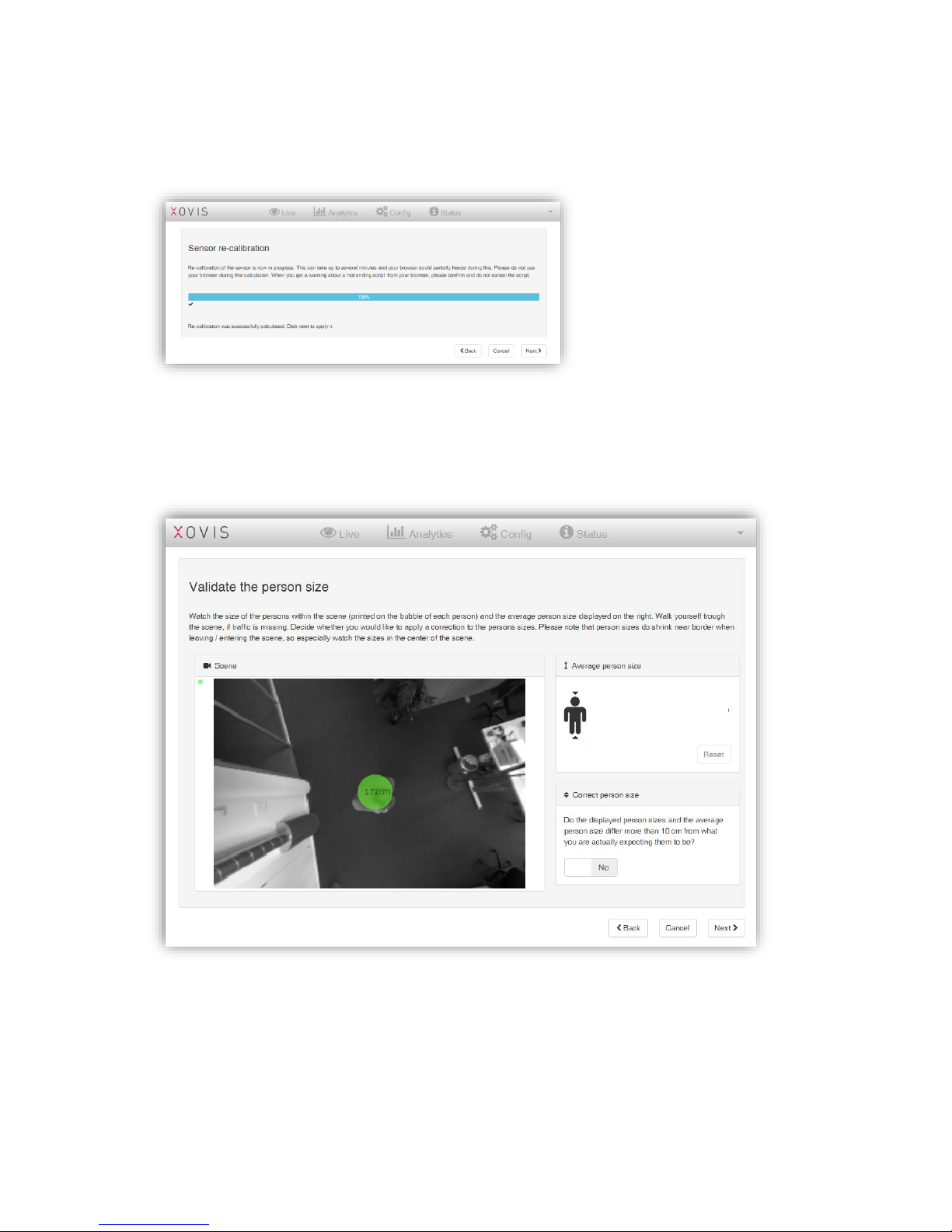
3.2.7.8 Validate the person size
In the succeeding screen, the user is asked to verify the person size. This is important to
validate the distance measurement of the sensor. In most cases, especially on mounting
heights below 3.5 meters, the person sizes will be quite exact without an additional
correction (precision is better than +/- 10 cm). But in several situations, the sensor might not
be able to correctly measure the scene and therefore measures the person sizes incorrectly.
If the average person size or the sizes printed on the bubbles within the scene seem to be
unrealistic, a correction can be applied. For this, the toggle switch in the “Correct person
172 cm
24 / 99 www.xovis.com
size” box on the right must be set to “Yes”. Now, using the slider, a size correction can be
applied (the resolution is 5 centimeter based as this is the accuracy range the sensor is
operating).
When modifying the slider, the correction is automatically applied to the scene, so the effect
can be observed immediately. Also the average person size is reset every time the slider is
moved.
Please note that person sizes do shrink near border when leaving / entering the scene, so
especially watch the sizes in the center of the scene. The average person size uses the
maximum height of each person detected within the scene, so it is more representative.
After verifying the person sizes, any correction is applied to the sensor after clicking “Next”.
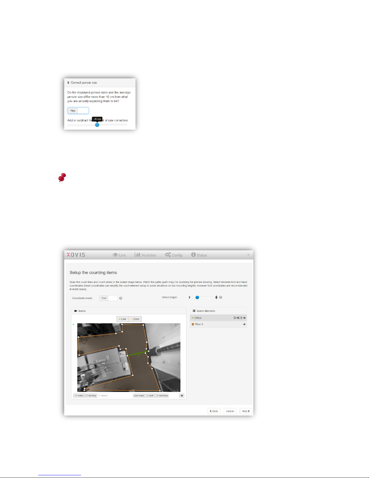
3.2.7.9 Setup the counting items
25 / 99 www.xovis.com
In the next screen, the counting setup can be performed. In the upper part of the screen, the
coordinate mode and the detect height can be set.
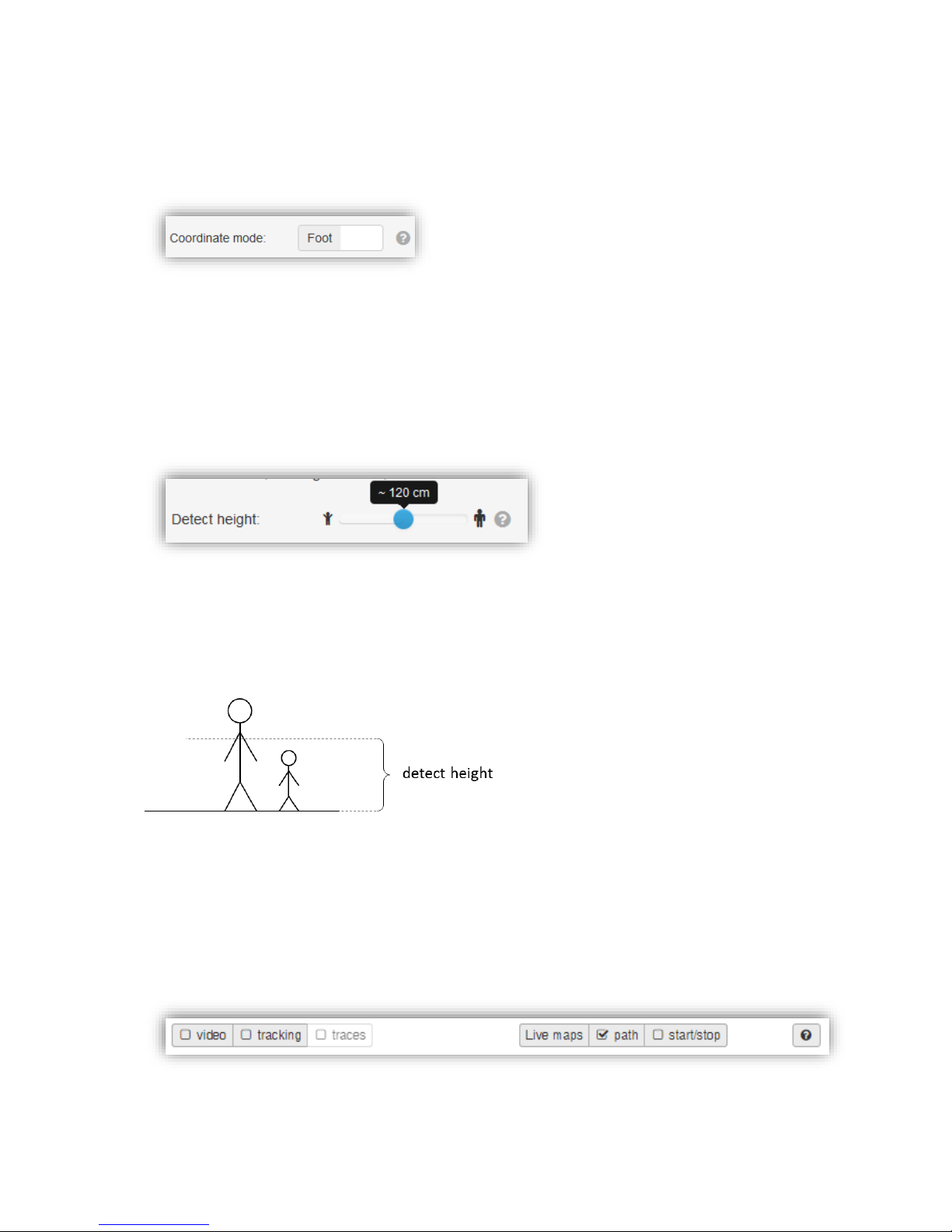
3.2.7.9.1. Coordinate mode
The coordinate mode defines where to show the tracking of a person, either at its head or at
its feet. The purpose of the coordinate mode and the difference between “head” and “foot” is
explained in detail in chapter 3.1.2.
When toggling between the two coordinate modes, the sensor will automatically apply the
changed mode and switch the displaying of the person positions accordingly.
3.2.7.9.2. Detect height
The detect height defines the height from floor, at which a person gets detected and analyzed
by the sensor. This parameter influences the detection of small persons (children) and can
be reduced to 80 cm at least. With this parameter the exclusion from persons below a
specific size can be realized, i.e. to ignore children from being counted. The detect height can
be parameterized between 80 cm and 160 cm. Figure 22 visualizes the detect height.
Figure 22: Detect height
When changing the detect height with the slider, the changes will automatically be applied to
the sensor so they can immediately be verified in the scene view.
3.2.7.9.3. Scene view controls
The scene view offers several controls which can be helpful when setting up the counting
elements.
The first control, the video checkbox, allows to activate or de-activate the live video.

26 / 99 www.xovis.com
The “tracking” checkbox controls whether to show a bubble on every tracked person. This
bubble will be located either on the person’s head or feet, depending on the chosen
coordinate mode (see chapter 3.2.7.9.1).
Figure 23: Bubble displayed on tracked person
The “traces” checkbox is only activated when the “tracking” checkbox is selected. If “traces”
is selected, the most recent part of the track of every person within the scene is visualized:
Figure 24: Displayed path of tracked person
The “Live maps” section allows to show/hide several types of visualization maps: If the
“path” checkbox is selected, the whole tracks of all persons are kept and visualized in the
scene image. This path map can be of great use while drawing the counting elements
properly as the displayed paths help the user to identify the areas where tracking actually
occurs:
Figure 25: Pathmap helps to identify the actual tracking while setting up the counting elements
27 / 99 www.xovis.com
Note: When the “path” checkbox gets unchecked, the tracks will disappear from the scene
view and be reset (when re-selecting the path live map checkbox, the old paths will not be
included again).
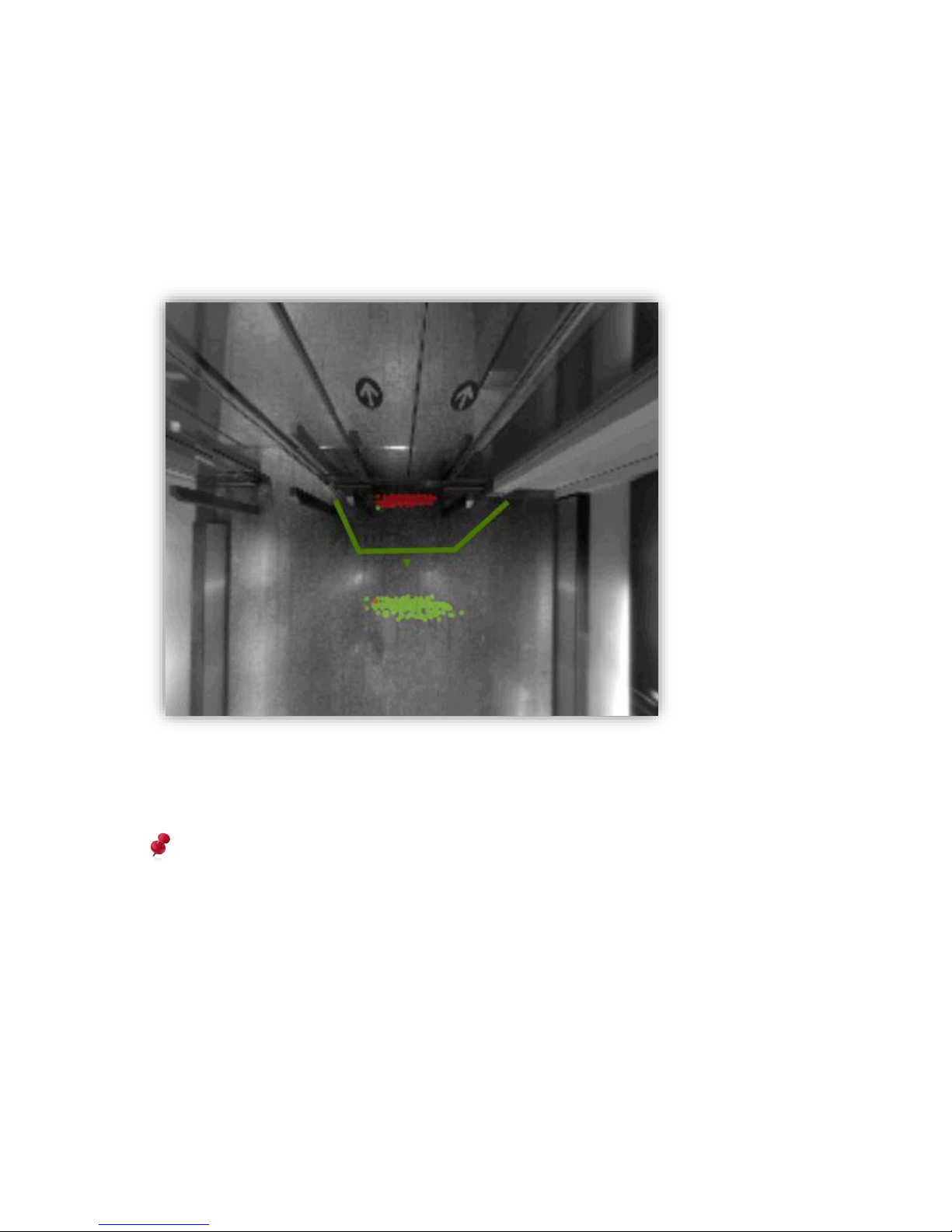
If the “start/stop” checkbox is selected, generation and deletion points of all persons will be
displayed as green and red dots. This allows to analyze, where people actually start to get
tracked and where they disappear again. Using this point map, a count line can be easily
adjusted properly to ensure to not miss any person.
Figure 26: Start/stop map visualizes generation and deletion points of persons
As with the path live map, when the “start/stop” checkbox gets unchecked, the points will
disappear from the scene and be reset.
Please note that all live visualizations are influenced by network bandwidth. As the
visualization are drawn by the client (web-browser) here, it is likely that some frames are
missed when low bandwidth is given. This leads to a visualization not showing the actual
truth, as, for example, start points will be drawn later as they actually occurred (location
will be more towards the inside of the scene).
Whenever using the maps for proper analytics, and especially with low bandwidth, it is
highly recommended to use the “visualization maps” instead, as they are based on
persisted, sensor-stored data. See chapter 3.2.9.2 for more details.
28 / 99 www.xovis.com
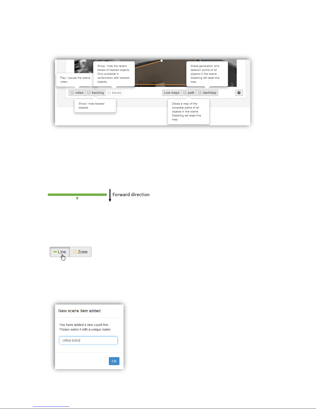
The help button offers quick explanations for all the control elements mentioned so far.
Hovering over it with the mouse will pop-up the help information:
3.2.7.9.4. Count lines
The count line is the first of the two counting and observation tools available with a PCSeries sensor. A count line measures the number of persons crossing a defined line.
Forward and backward crossings are counted separately. A line therefore has a directional
property, i.e. an orientation. This orientation is indicated with a centered arrow pointing in
the direction of forward crossing (see Figure 27).
Figure 27: Orientation of a count line
A count line offers several ways to analyze person crossings for its counts. These strategies
are explained in section “Example Situations” in chapter 3.2.7.9.7 “Count line configuration”.
Drawing a count line
A line can be drawn by selecting the drawing tool “Line” and directly drawing the corners of
the line in the scene image. A line is finished with a second click on the last corner, by a
double click to create the last corner, by disabling the drawing tool “Line” or by pressing
[Esc] on the keyboard. After finishing a line, the user is asked to name it.
29 / 99 www.xovis.com
As with the floor masks, this name must be unique among all other scene elements. After
naming the line it is automatically added to the scene element list.
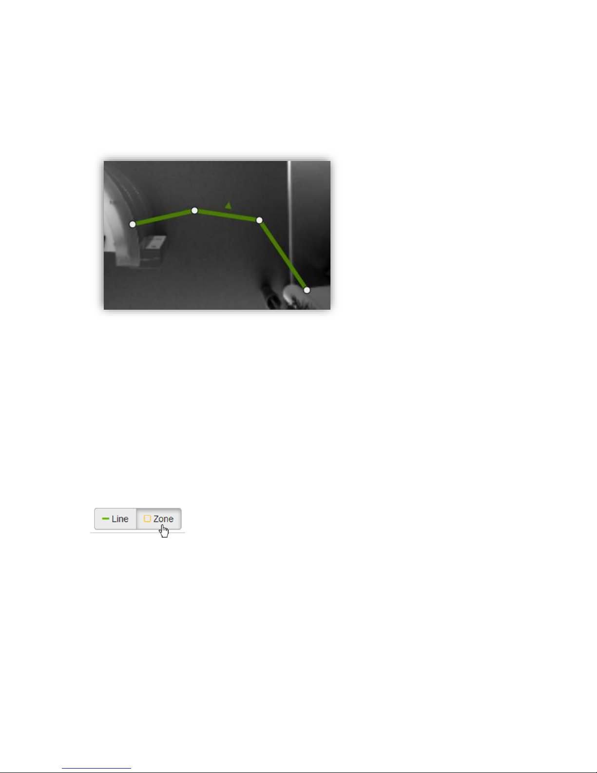
In the examples shown above, a line always has two corners / points. However, a line can
have multiple points (corners) to fit all situations. Such a multi-point line can be created by
just going ahead drawing corner points in the scene. Figure 28 shows an example:
Figure 28: A multi-point line
An existing line can be modified by moving its corners or by dragging the whole line by
clicking-and-holding on a line edge.
The sensor supports up to 8 count lines. When the 8th line is drawn, the line drawing tool gets
disabled. One or more lines then need to be deleted to re-enable the line drawing tool.
3.2.7.9.5. Count zone
The count zone is the second counting and observation tool available with the PC2. A count
zone measures the occupancy of a defined zone. Every count zone provides a count level
which indicates the number of persons currently situated within the zone.
Drawing a count zone
A count zone can be drawn similar to the floor mask. By selecting the drawing tool “Zone”
one can simply draw the corner points of the zone polygon in the scene image. A count zone
can be finished by clicking on the first corner again, by double-clicking to create the last
corner, by disabling the “Zone” tool or by pressing [Esc] on the keyboard. As with the count
lines, after finishing, the user is asked to name the count zone before it gets automatically
added to the scene element list.
30 / 99 www.xovis.com
Figure 29: A count zone
Editing a count zone is the same as with the floor masks.
The sensor supports up to 8 count zones. When the 8th zone is drawn, the zone drawing tool
gets disabled. One or more count zones then need to be deleted to re-enable the zone
drawing tool.
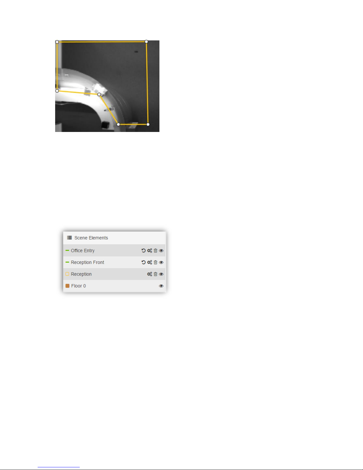
3.2.7.9.6. Scene elements
All the scene elements described so far (floor masks, count lines, count zones) are listed in
the scene elements box:
Figure 30: Scene elements
When hovering over the elements within the list, the element gets hightlighted both within
the list and within the scene. When clicking on a specific element, it gets marked red both
within the list and within the scene. At the same time the selected element is brought to the
front of the scene view, allowing to modify it even if it was actually lying behind another
element (e.g. count line behind a count zone). Clicking again on the element or selecting
another element will unmark it again. The vice-versa procedure is also supprted, i.e.
hovering and selecting the scene elements within the scene view. Figure 31 shows an
example:
 Loading...