

Page 1
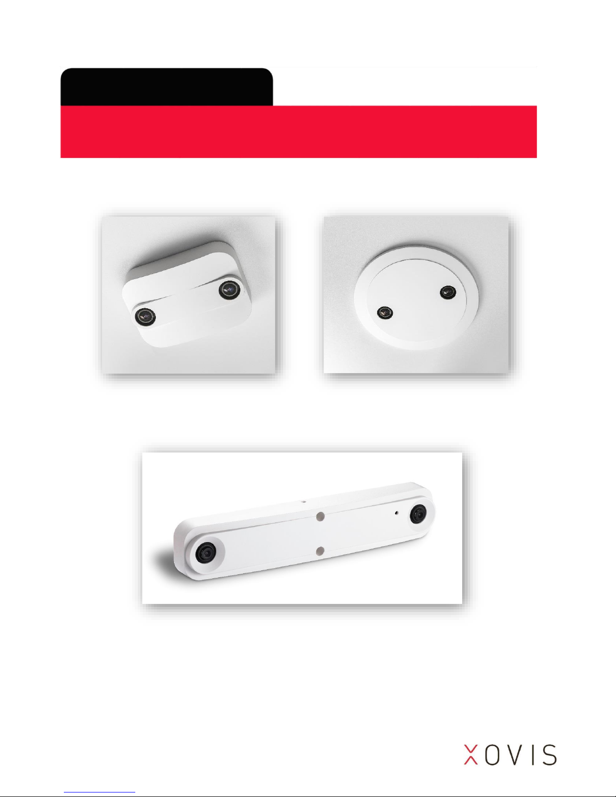
PC-Series
User manual
Page 2
Copyright reminder
Copyright © 2016 by Xovis AG, Switzerland.
All rights reserved. No part of this publication may be reproduced, stored in a retrieval
system, or transmitted, in any form by any means, electronic, mechanical, photocopying,
recording, or otherwise, without the prior written permission of the publisher. Printed and
published in Switzerland.
While Xovis AG believes the information included in this publication is correct as of the date
of publication, it is subject to change without notice.
All cited trademarks and registered trademarks are the property of their respective owners.
Non-disclosure reminder
All information in this document is strictly confidential and may only be published by Xovis
AG, Switzerland.
Document history
Version
Date
Author
Comment
1.0
17.11.2014
CG / FLM
First Release
1.1
27.03.2015
CG
Updates for SW release 2.2
1.2
16.04.2015
CG
Updates for SW release 2.2.1
1.3
30.06.2015
CG
Updates for SW release 2.3.1
1.4
22.07.2015
CG / FLM
Mounting instructions now described
in separate document
1.5
29.09.2015
CG / FLM
Updates for SW release 3.0.1
1.6
30.10.2015
CG / FLM
Updates for SW release 3.1.0
1.7
23.12.2015
CG
Updates for SW release 3.2.0
1.8
12.06.2016
CG
Updates for SW release 3.3.0
1.9
22.12.2016
CG
Updates SW release 3.4.0
Page 3
Table of contents
1 Overview ................................................................................................... 5
Content Declaration ...............................................................................................5
PC-Series hardware concept ..................................................................................5
PC-Series 3D sensor ................................................................................................5
2 Installation Fundamentals ......................................................................... 6
Network requirements ...........................................................................................6
Power over Ethernet ...............................................................................................6
Sensor LED ..............................................................................................................6
3 Configuration & Usage ............................................................................. 7
Person tracking .......................................................................................................7
3.1.1 Person generation ........................................................................................................ 7
3.1.2 Person position / coordinate mode ............................................................................. 8
Setting up a sensor .................................................................................................9
3.2.1 Introduction ................................................................................................................. 9
3.2.2 Setting up the sensor in the network .......................................................................... 9
3.2.3 Xovis Sensor Explorer ................................................................................................. 10
3.2.4 Access the web interface ........................................................................................... 14
3.2.5 Login to the sensor .................................................................................................... 15
3.2.6 Navigation .................................................................................................................. 15
3.2.7 Setup Wizard .............................................................................................................. 17
3.2.8 Live View .................................................................................................................... 42
3.2.9 Analytics View ............................................................................................................ 48
3.2.10 Config View ................................................................................................................ 57
3.2.11 Status View ................................................................................................................. 82
3.2.12 Firmware upgrade ...................................................................................................... 84
3.2.13 Extended analytics ..................................................................................................... 86
3.2.14 Configuration changes from another client ............................................................... 87
3.2.15 Connection warning ................................................................................................... 88
4 Troubleshooting ...................................................................................... 89
False behavior ....................................................................................................... 89
Masks .................................................................................................................... 89
4.2.1 Exclusion masks ......................................................................................................... 89
4.2.2 Taboo masks .............................................................................................................. 90
4.2.3 Example for mask differentiation ............................................................................... 92
Page 4

Placement of dwell zones ..................................................................................... 93
Time synchronization mechanism ....................................................................... 95
5 Technical data ......................................................................................... 97
6 Certificates / Tests ................................................................................... 98
7 Custom Integration ................................................................................. 99
API ......................................................................................................................... 99
Plugin Architecture ............................................................................................... 99
Page 5
5 / 99 www.xovis.com
1 Overview
Content Declaration
This manual is intended for administrators and users of the PC-Series sensor and is
applicable for software version 3.3.0 and later. It includes instructions for installing, using
and managing the sensor on your network. Basic knowledge of network configuration and
knowledge of the specific network in which the sensor is operated are required when using
this product. Later versions of this document will be published in the customer section on
the Xovis website at www.xovis.com.
PC-Series hardware concept
The housing of a PC-Series sensor is designed to be mounted directly on the ceiling. Xovis
offers several accessories allowing different installation alternatives. Please refer to the
accessory overview and the mounting instruction showing all versions.
The housing has two holes for sensor positioning and fixation. The Ethernet connector is on
the backside.
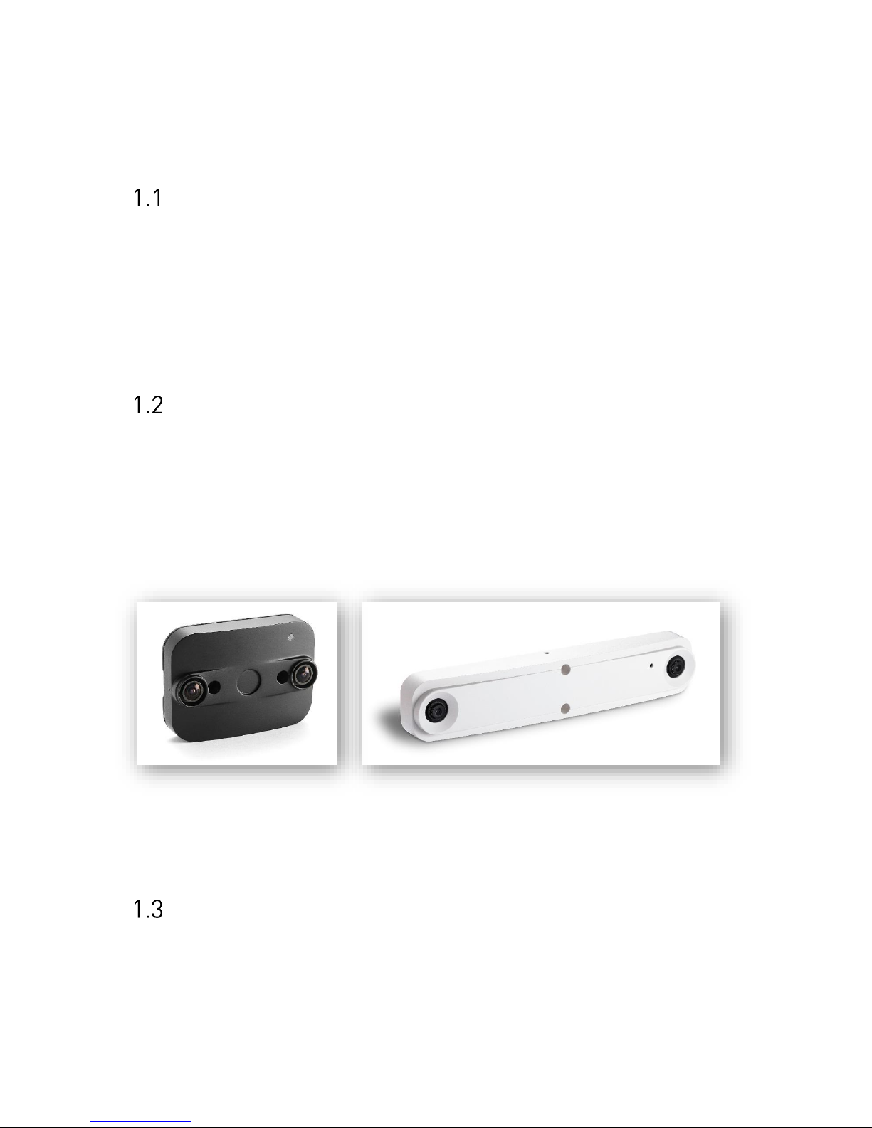
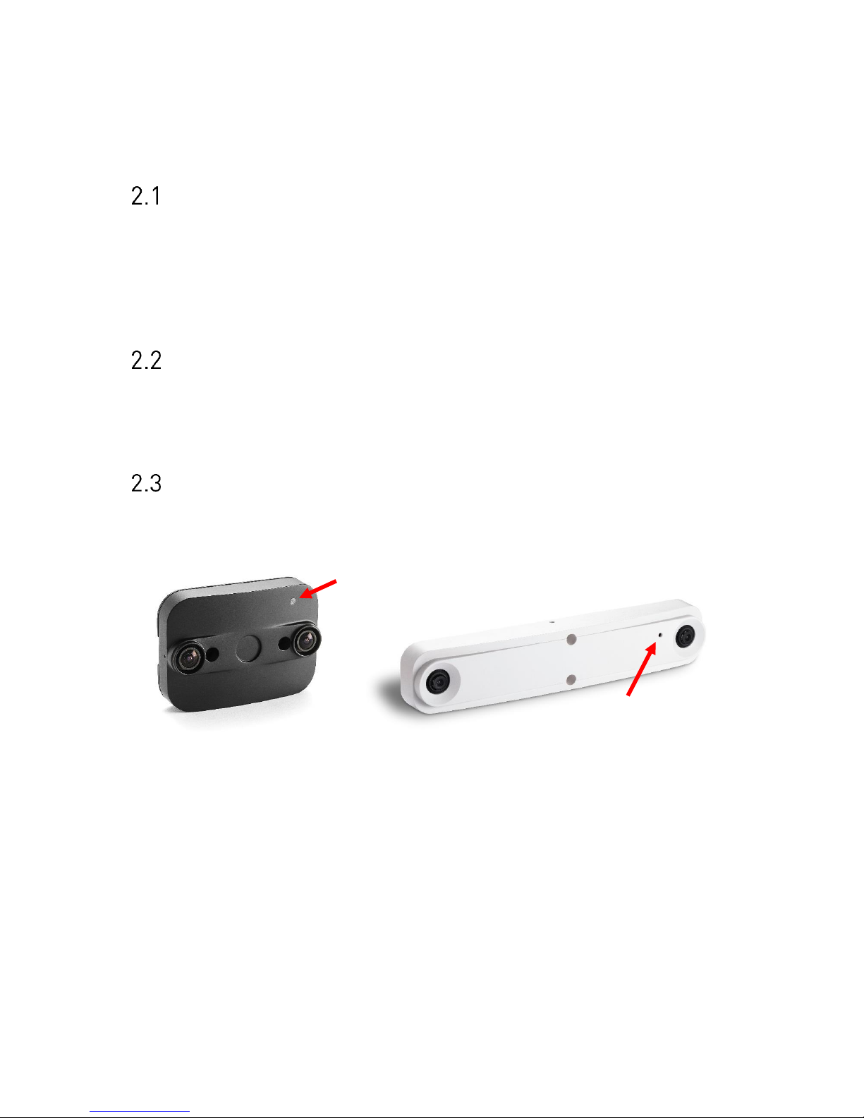
Figure 1: PC2 (left) and PC3 (right) 3D sensor
PC-Series 3D sensor
The PC2 3D sensor comes in a black metal housing and supports ceiling heights up to 6.0m.
The PC3 3D sensor comes in a white metal housing and supports ceiling heights up to 20m.
Page 6
6 / 99 www.xovis.com
2 Installation Fundamentals
Network requirements
The device needs to be connected to the network by a shielded Cat 5 RJ45 Cable. The plug
and the sensor need to be free from any mechanical pressure. The sensor supports Ethernet
10/100Mb Full/Half/Auto negotiation based on the IEEE 802.3 standard. It is highly
recommended to set the switch port to auto negotiation.
Power over Ethernet
The sensor is powered by PoE Class 0 compliant to IEEE 802.3af. As defined by the standard,
the network switch port needs to provide 15 Watts at 48 V.
Sensor LED
The PC-Series sensor provides a multifunctional LED on the front side. The red arrow on the
next picture indicate the LED on the PC2 and PC3 models.
Figure 2: PC2 LED (left) and PC3 LED (right)
The LED indicates the following states:
- Green: Device is powered by PoE
- Orange/Green blinking: Device is up and running
The LED state can be useful during installation. When using the optional housing, the LED
will be covered after successful mounting.
Page 7
7 / 99 www.xovis.com
3 Configuration & Usage
Person tracking
The Xovis PC-Series sensor tracks persons. A few things have to be taken into account to
understand how the detection and tracking of persons works:
3.1.1 Person generation
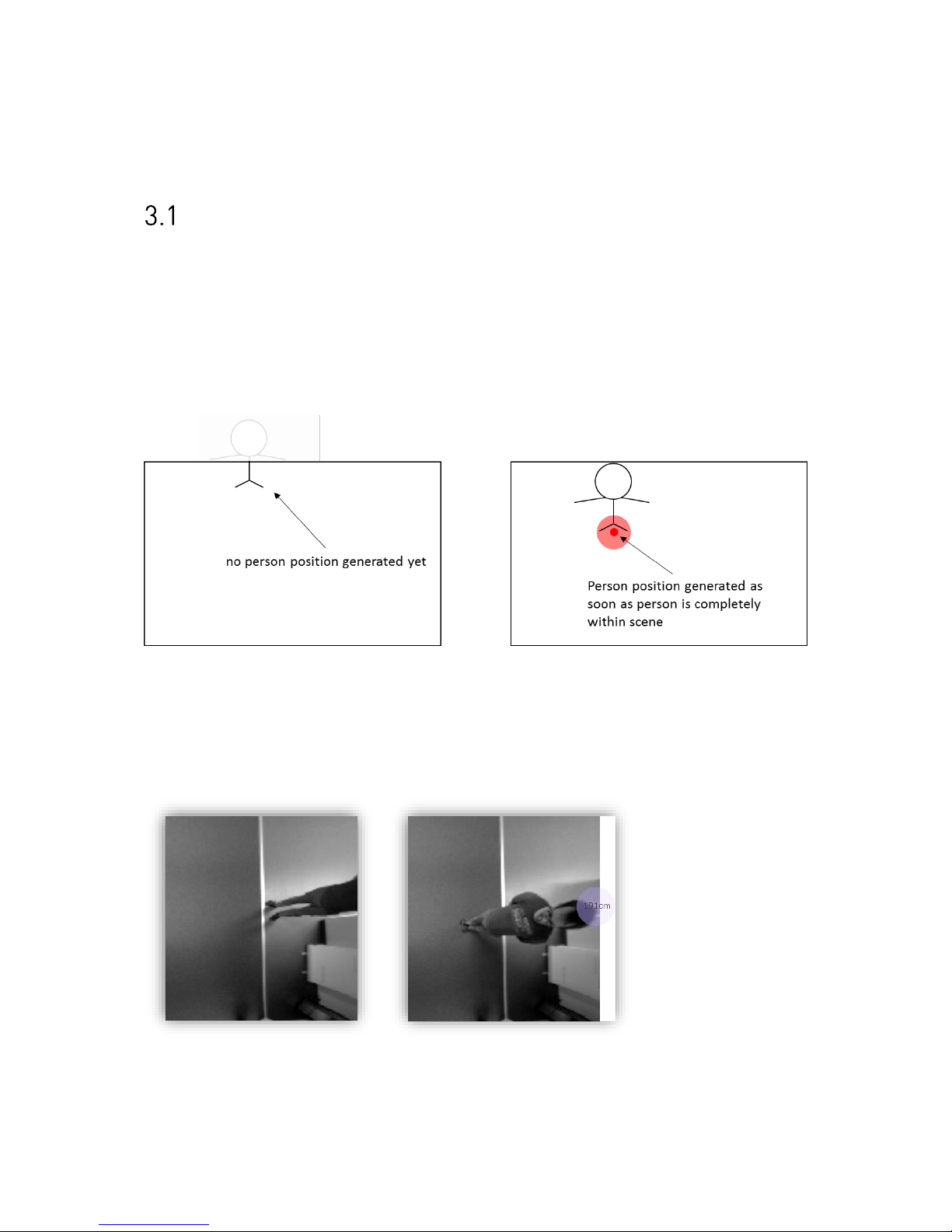
The PC-Series sensor generates a person first when the person is completely within the
visible scene (see Figure 3).
Figure 3: Person generation
When a person track once was generated, the person stays tracked until it leaves the scene
again and its head is touching the visible scene border. Tracking/counting at border is
therefore not supported for persons only partially within the scene.
The following situation illustrates the person generation capability:
Figure 4: Demonstration of person generation with coordinate mode “head”
The situation shows that a person is first detected by the sensor when its head is completely
visible i.e. within the scene.
Page 8
8 / 99 www.xovis.com
3.1.2 Person position / coordinate mode
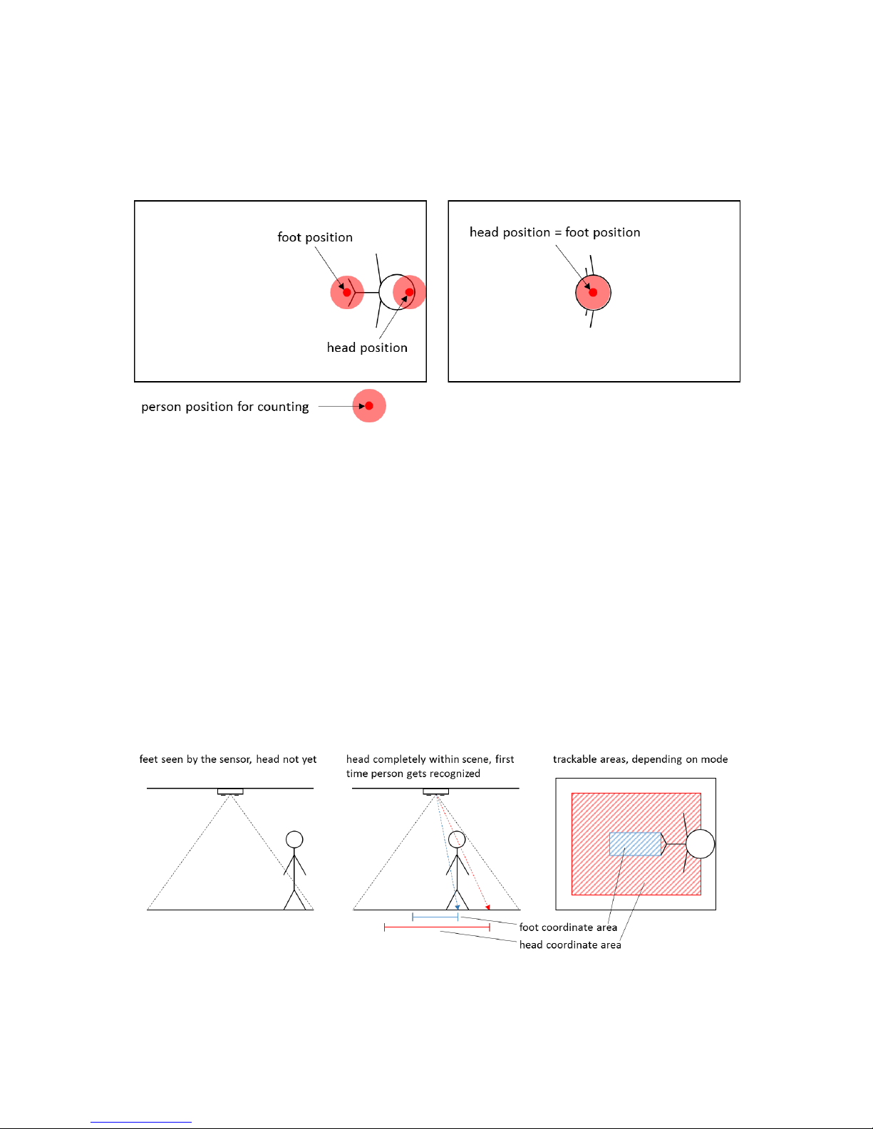
The PC-Series sensor uses one specific position per person to evaluate the counting on lines
and zones. This position is either located at the head of a person or at its feet. Figure 5
illustrates the two possible positions.
Figure 5: Person position
Due to the visual perspective of the overhead mounted sensor, the head and foot positions
are congruent directly underneath (in the plump) of the sensor but at different positions at
the scene borders. The user can choose which position shall be used on the sensor by
defining the coordinate mode. This coordinate mode, which can either be “foot” or “head”,
then defines where to show the tracking of a person.
The displaying of the person tracks (paths) on the other hand influences the definition of the
counting elements: When choosing foot coordinates, the person paths will first be displayed
after an offset from the border, as persons get detected by the sensor first, when their head
is seen by the sensor. And, due to the visual perspective, the feet of a person will be seen by
the sensor long before the head of the same person is seen. Or, in other words, when a
persons head is seen by the sensor, its feet will be located within the sceen with a certain
distance to the border / to the head of the person. The following situation demonstrates this
fact:
Figure 6: Different tracking areas depending on the coordinate mode
Page 9
9 / 99 www.xovis.com
Theoretically the foot coordinates will always be the easier way to use, as all counting items
(e.g. count line) can then just be oriented on the scenes floor (all possible locations of a
persons feet are given by considering the floor of the scene). But due to the visual
perspecitive, feet positions will not be displayed within the complete visible floor which can
complicate the proper drawing of counting items, especially on lower mounting heights
where the difference between the trackable areas of both coordinate modes is quite big (see
Figure 6). Therefore, in some situations, head coordinates can be the preferred choice.
The following situation illustrates the two different coordinate positions:
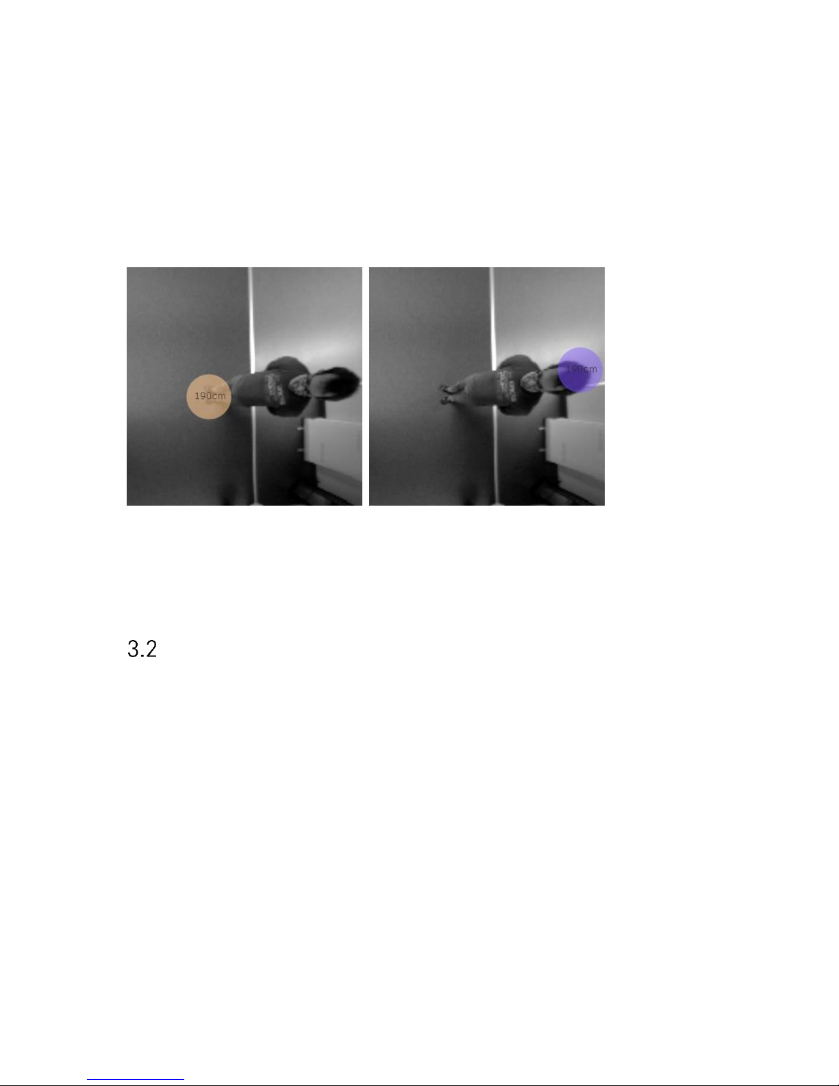
Figure 7: Demonstration of coordinate modes
In the left image, foot coordinates are in use. In the right image, head coordinates are in use.
The situation shows that the first possible position of person “bubbles” is clearly closer at
the border when using head positions.
Setting up a sensor
3.2.1 Introduction
This chapter describes the recommended procedure how to set up a new PC-Series sensor.
3.2.2 Setting up the sensor in the network
The sensor is setup for use in a DHCP environment by default. If a sensor is attached to a
network, it is expecting an IP address assignment by a DHCP server in the network. This is
the simplest way to install a new sensor.
If no DHCP server is present, a static IP setting needs to be applied to the sensor. For this
purpose, a Windows PC attached to the same physical subnet as the sensor is required. The
static network settings can then be applied with the Xovis Sensor Explorer tool, which is
described in the next chapter.
Page 10
10 / 99 www.xovis.com
3.2.3 Xovis Sensor Explorer
The Xovis Sensor Explorer tool offers a simple way to install and manage Xovis sensors in the
network.
3.2.3.1 Discover sensor on the network
The Xovis Sensor Explorer can be run without installation directly by double-clicking the
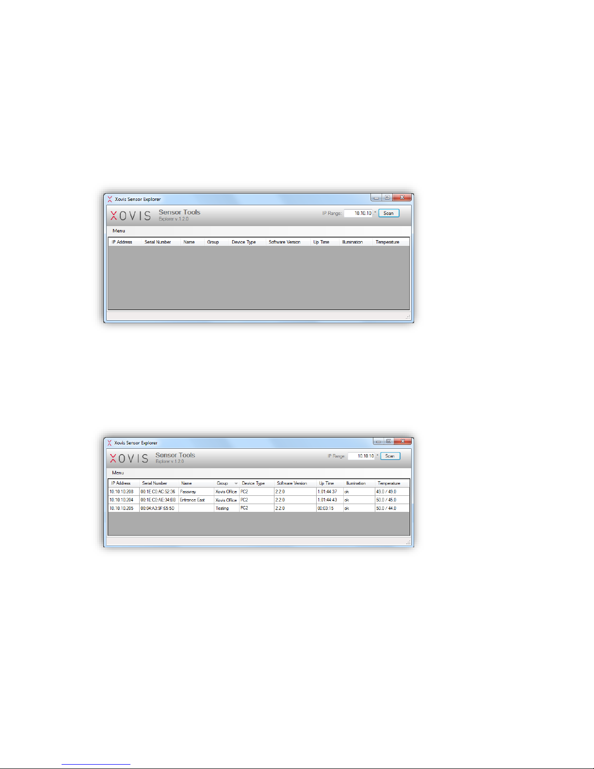
XovisSensorExplorer.exe file. The following screen shows up:
Figure 8: Xovis Sensor Explorer
On the top right of the screen, an IP range can be specified. This range will be scanned for
Xovis sensors when clicking on the “Scan” button. Every sensor properly configured in the
specified IP subnet will be discovered and listed in the Xovis Sensor Explorer. Figure 9
shows an example:
Figure 9: Found sensors on the network
Page 11
11 / 99 www.xovis.com
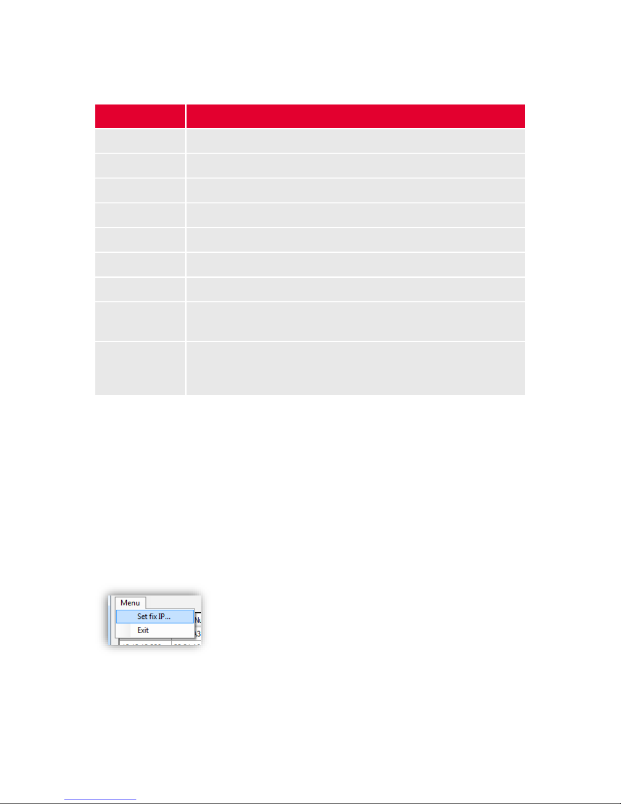
For all discovered sensors the Xovis Sensor Explorer will display a series of information
which can be useful for maintaining the Xovis sensors in a network:
Item
Description
IP Address
The sensors IP address
Serial Number
Serial number of the sensor
Name
The sensor name, if set
Group
The sensor group, if set
Device Type
The type of the sensor (e.g. PC2, PC2-UL, PC3)
Software Version
The version of the software currently running on the sensor
Up Time
The sensors uptime in the format d.hh:mm:ss
Illumination
The illumination status of the scene in which the sensor is operating,
can be “ok” or “insufficient”
Temperature
The sensors temperature in degrees Celsius whereby the first number
represents the sensors housing temperature and the second number
the sensors internal temperature
3.2.3.2 Installing a sensor in a fix IP environment
The Xovis Sensor Explorer will only display sensors properly configured and reachable on the
network. In a fix IP environment, a newly attached sensor needs to be setup with a valid IP
configuration first to be able to get discovered by the Xovis Sensor Explorer (the default IP
address of the sensor when no DHCP is in use is 192.168.1.168). For this purpose, the Xovis
Sensor Explorer allows to temporarily apply a specific IP setting to any sensor physically
attached to the same subnet, regardless of whether the sensor was already discovered and
therefore displayed in the Xovis Sensor Explorer list or not, just by specifying the sensors
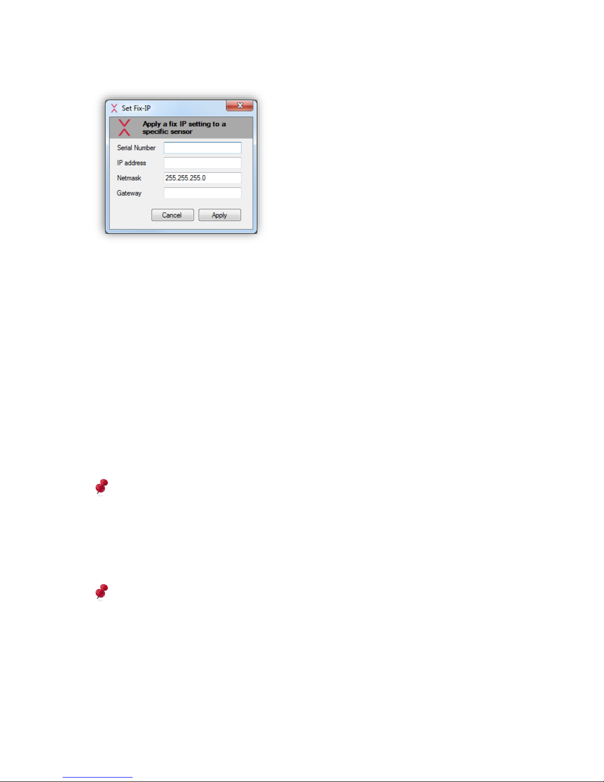
serial number and the desired network configuration. The menu located directly beneath the
Xovis lettering in the top left of the screen contains the menu item “Set fix IP…” (see Figure
10).
Figure 10: Set fix IP menu item
Page 12
12 / 99 www.xovis.com
By clicking it, the following dialog appears:
Figure 11: Set Fix-IP dialog
In the first field, the serial number of the sensor needs to be specified. The correctness of
this number is very important and needs to be in the format XX:XX:XX:XX:XX:XX (X to be
replaced). The serial number can be found on the back side of the sensor or on the package
in which the sensor was delivered.
In the fields “IP address”, “Netmask” and “Gateway”, the desired network settings need to be
specified, i.e. the fix IP settings to be applied on this sensor. All fields are required. When
pressing “Apply”, the specified settings are sent to the sensor and a message informs the
user to be patient for 20 seconds. After this time, the sensor should have come up with the
new IP settings.
If the PC running the Xovis Sensor Explorer is located in the same IP range or allows routing
to the IP range of the previously configured sensor, the Xovis Sensor Explorer is now able to
discover the sensor when specifying the proper IP range and clicking again on the “Scan”
button.
The sensor needs to be attached to the same physical subnet as the Windows PC running
the Xovis Sensor Explorer.
As the static IP was only set temporarily and will be lost with the next reboot of the sensor it
is now important to apply the desired IP settings permanently using the web interface (see
following chapters).
After temporarily applying a static IP with this procedure, it is important to permanently
set the fixed IP-address in the web interface afterwards!
Page 13
13 / 99 www.xovis.com
3.2.3.3 Setting a fix IP address to a discovered sensor
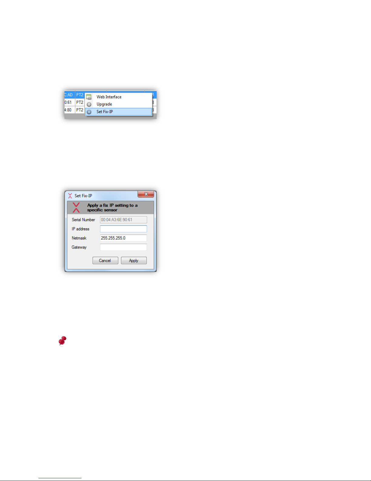
The Fix-IP dialog (see chapter “3.2.3.2 Installing a sensor in a fix IP environment”) can also
be opened for any sensor already discovered by the Xovis Sensor Explorer by simply rightclicking on it in the list and choosing “Set Fix-IP” in the popping up menu (see Figure 12).
Figure 12: Set Fix-IP
The same dialog as described in chapter 3.2.3.2 shows up with the single difference that the
serial number field is already filled with the one of the selected sensor. The remaining fields
again request the user to specify the IP address, the subnet mask and the gateway for the
specific sensor:
Figure 13: Set Fix-IP dialog
After applying the IP settings to the sensor by clicking the “Apply” button, the specified
settings are sent to the sensor and a message informs the user to be patient for 20 seconds.
After this time, the sensor should have come up with the new IP settings and can be found in
the according network and IP range.
After temporarily applying a static IP with this procedure, it is important to permanently
set the fixed IP-address in the web interface afterwards!
3.2.3.4 Upgrading a sensor
A sensors software / firmware can be upgraded by right clicking on a specific sensor in the
list of the Xovis Sensor Explorer and choosing “Upgrade” in the appearing dropdown menu.
In the appearing file dialog, an upgrade file of the type “xfw” (file extension) needs to be
selected. After applying a valid upgrade file, the sensor will instantaneously start with the
upgrade procedure which usually takes about 3 minutes. When refreshing the list of sensors
in the network by clicking again on the “Scan” button of the Xovis Sensor Explorer after these
3 minutes, the upgraded sensor will appear with updated software version.
Page 14
14 / 99 www.xovis.com
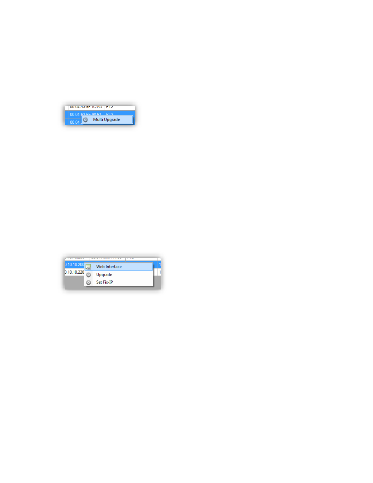
An upgrade can also be applied to multiple sensors at the same time by selecting all or a
part of the sensor in the list of the Xovis Sensor Explorer with [Ctrl] + [A] or pressed [Ctrl]
and left mouse click on the desired sensors. A right click on the selection opens a popup
menu with the only item “Multi Upgrade” (see Figure 14). Clicking it opens the same file
dialog as for upgrading a single sensor but will distribute the chosen upgrade file to all
selected sensors at the same time when applying.
Figure 14: Multi Upgrade
A sensors software / firmware can also be upgraded via its web interface. This procedure is
described in chapter 3.2.12.
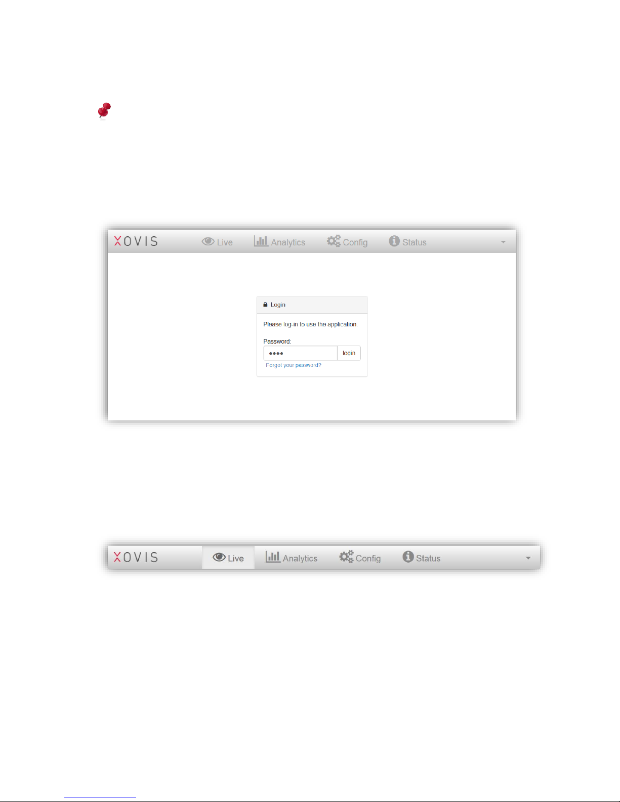
3.2.4 Access the web interface
The sensor web interface is accessed by typing its IP address directly into a web browser on
a PC connected to the same network as the sensor. Alternatively, the sensors web page can
be opened by double-clicking a sensor in the Xovis Sensor Explorer or by clicking the menu
item “Web Interface” in the popup menu appearing when right-clicking on a sensor in the
Xovis Sensor Explorer (see Figure 15). The web page will be opened in the default browser of
the operating system.
Figure 15: Menu item “Web Interface” in Xovis Sensor Explorer
3.2.4.1 HTTPS
The sensor web interface can also be accessed over HTTPS by just declaring the protocol
accordingly (https://).
3.2.4.2 Supported browsers
The sensor user interface is an HTML/JavaScript based website. The following web browsers
offer a proper functionality of the website:
- Firefox 4 or newer
- Google Chrome version 10 or newer
- Microsoft Internet Explorer version 10 or newer
- Apple Safari version 5 or newer
- Opera version 12 or newer
Page 15
15 / 99 www.xovis.com
Recommended browsers are Firefox, Chrome, Opera and Internet Explorer.
For all browsers JavaScript support needs to be enabled and all caching for this website
needs to be switched off!
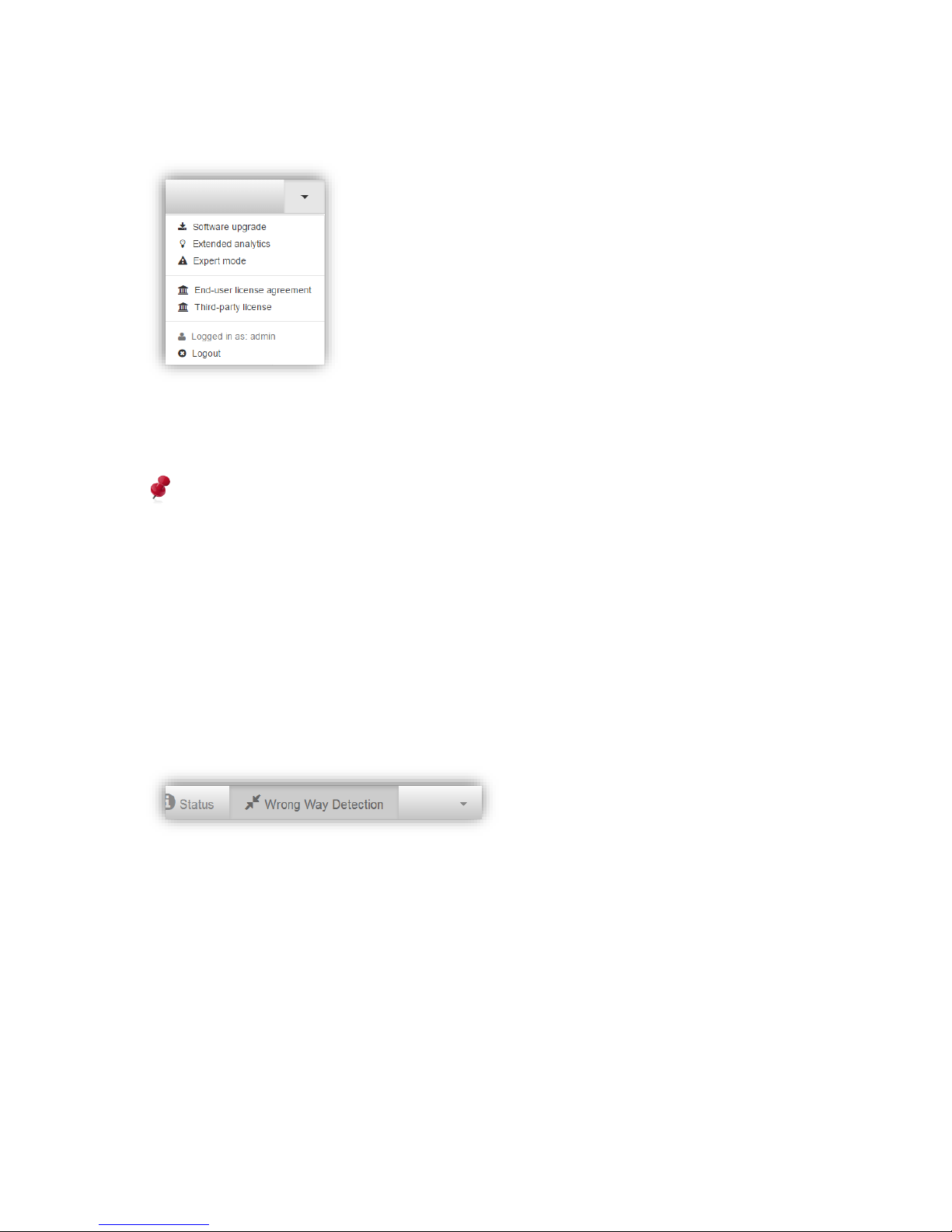
3.2.5 Login to the sensor
The arrival page of the website shows a log-in dialog. The default password is “pass”
(without the “”).
Figure 16: Login screen
The login screen holds a “Forgot your password” link. This allows to reset the sensor using
the Sensor Master Key (SMK). The reset procedure is described in chapter 3.2.10.4.5.
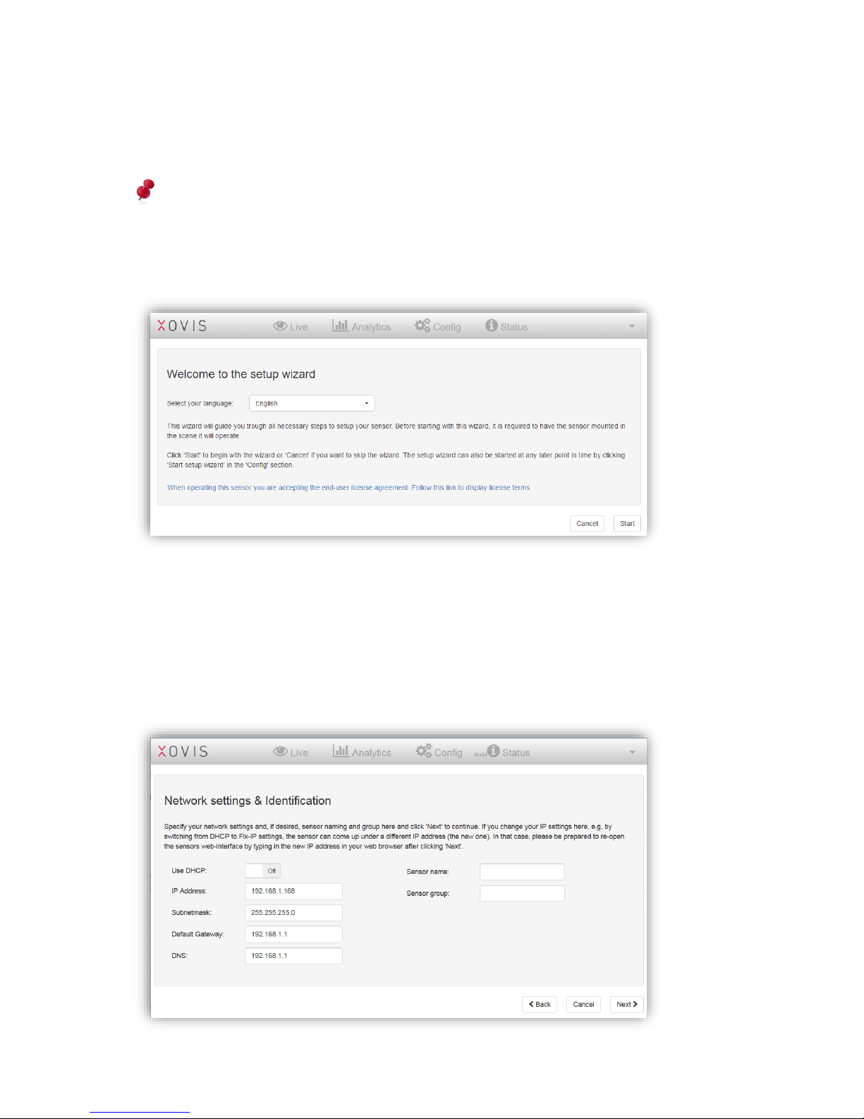
3.2.6 Navigation
The navigation bar is located at the top of the web GUI. It basically holds three sections: The
logo, the menu buttons and a context menu.
The menu buttons allow the user to switch between the four main views “Live”, “Analytics”,
“Config” and “Status”. The purpose of these views is described in their respective chapters
3.2.8 to 3.2.11. These buttons are disabled when logged out and in the setup wizard mode
(see next chapter).
Page 16
16 / 99 www.xovis.com
The context menu holds additional functionalities for maintaining the sensor and to logout
the current user:
The “Software Upgrade” procedure will be explained in chapter 3.2.12. “Extended Analytics”
is covered in chapter 3.2.13. The “Expert Mode” is not documented in this manual as it is
reserved for expert use only.
Xovis strongly recommends to NOT USE the expert mode at all as changes made with the
expert mode can cause the sensor to become unresponsive.
The two entries for EULA and third-party licenses display the respective licenses.
The “Logout” button ends the session of the currently logged in user and returns to the login
page. The currently logged in user is displayed directly above the “Logout” button.
3.2.6.1 Plugins
The PC2 sensor can be enriched with various plugins. The plugin installation procedure is
described in chapter 3.2.10.4.3. Plugins which offer a frontend component will also be listed
in the navigation bar. Figure 17 shows an example with the “Wrong Way Detection” plugin:
Figure 17: Plugin button in the navigation bar
A plugins functionality and usage is documented in the documentation of the specific plugin.
Page 17
17 / 99 www.xovis.com
3.2.7 Setup Wizard
As long as the sensor is not configured, the setup wizard will be shown directly after loggingin.
It is strongly recommended to use the setup wizard for setting up the sensor as the wizard
ensures to gather all information needed for a proper usage of the sensor.
3.2.7.1 Welcome screen
Figure 18: Setup wizard
The welcome screen of the wizard gives a quick description of the intent of the wizard and
allows the user to choose the desired GUI language. The wizard can be started by clicking
“Start”. At any step of the wizard, it can be ended by clicking “Cancel”. The setup wizard can
be re-started anytime in the config view (see chapter 3.2.10.1.3).
3.2.7.2 Network settings & Identification
Page 18
18 / 99 www.xovis.com
As first step, the wizard is asking for the network settings and identification naming. The
sensor can be run with DHCP or a fix IP address. If not using DHCP and the IP settings have
been applied already by using the Xovis Sensor Explorer (see chapter 3.2.3.2), it is
recommended to double check the network settings here. Optionally, a name and group can
be specified for the sensor. By clicking “Next”, the network settings are applied to the
sensor.
If the IP address of the sensor is changed here, the sensor will instantaneously come up
under the new address after pressing “Save”. In that case the new IP address needs to be
entered in the web browser after saving.
3.2.7.3 Date & Time
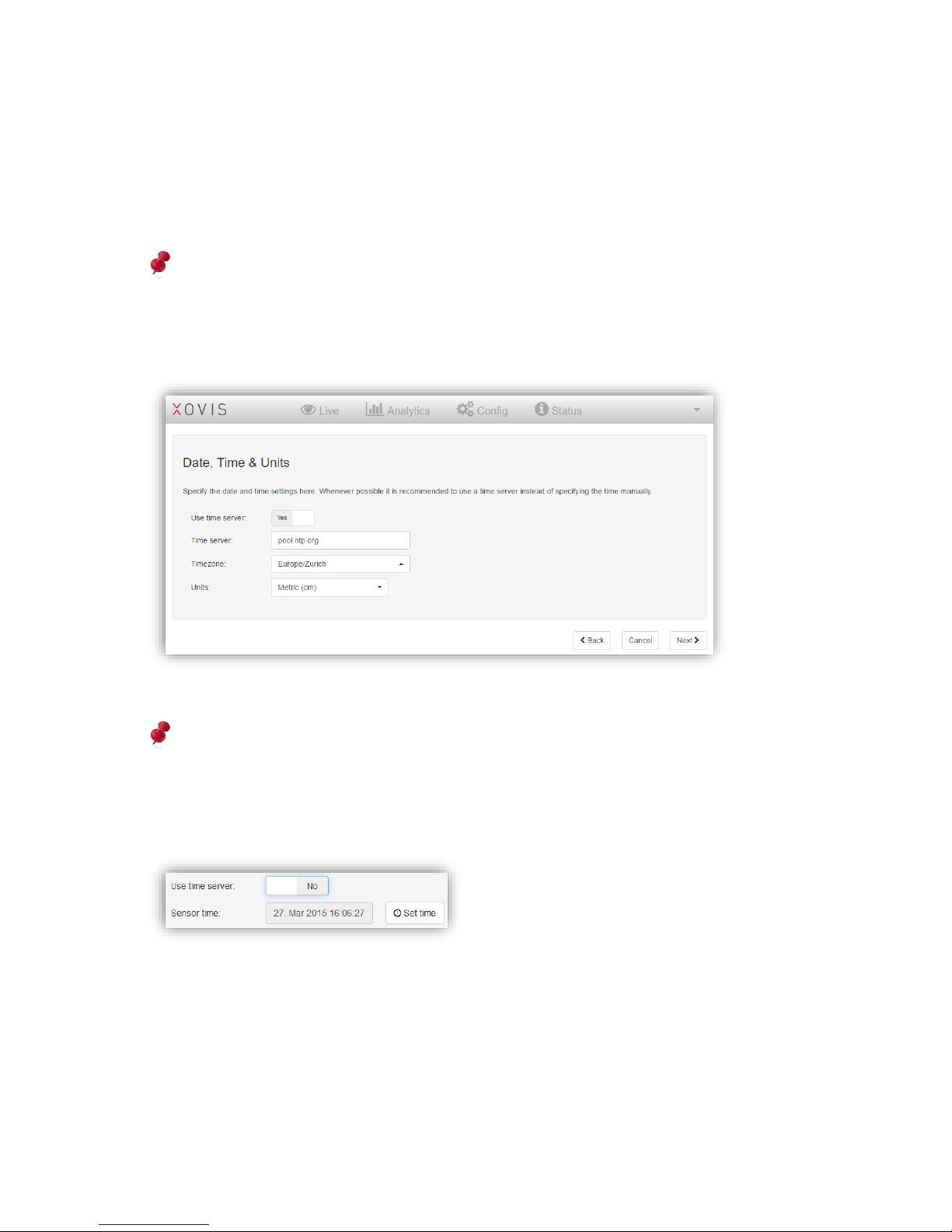
In the next screen the wizard is asking for setting the sensors date, time and units.
Whenever possible it is recommended to use a timeserver, as a correct time can be
crucial for stored counting data statistics.
When not using a time server, the sensor time can be set manually by switching the “Use
time server” toggle to “No” and then clicking on “Set time”:
The time zone dropdown is ordered by continents / geographic regions and cities. The time
zone should be set according to the sensors location.
The “Units” dropdown allows to choose between Metric (cm) and Imperial (feet/inch) units.
By clicking “Next”, the date and time settings are applied to the sensor.
Page 19
19 / 99 www.xovis.com
3.2.7.4 Sensor settings I
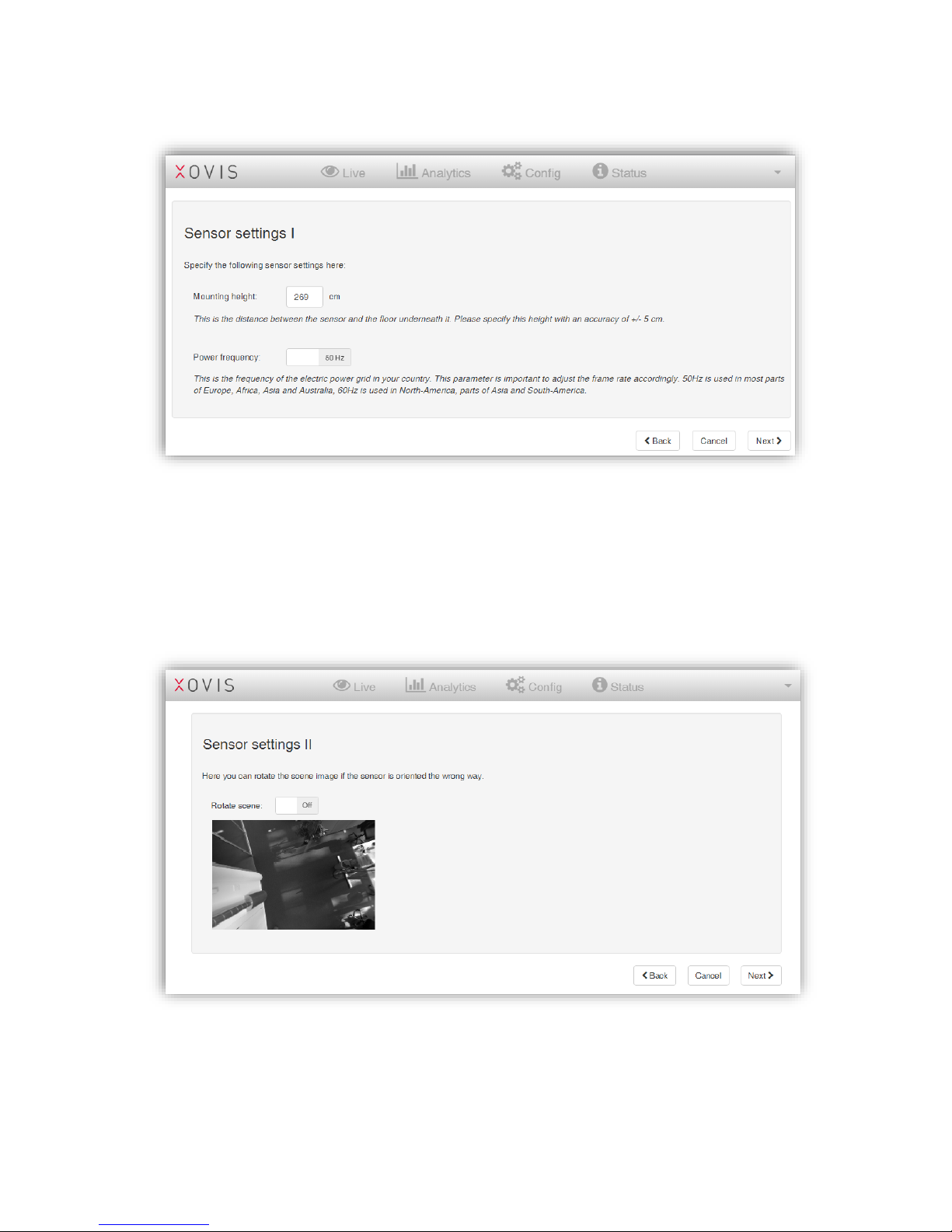
In the next screen, some base settings for the sensor operation need to be specified. First,
the mounting height needs to be set as accurate as possible. Second, the user is asked to
specify the power frequency of the country of operation. This is needed to adjust the sensors
frame rate to the illumination frequency. By clicking “Next”, these settings are applied to the
sensor.
3.2.7.5 Sensor settings II
In the succeeding screen, the scene image can be rotated by 180 degrees if desired. This can
be of use if the user’s sense of the scene view differs from the orientation of the mounted
sensor. The orientation is applied by clicking “Next”.
Page 20
20 / 99 www.xovis.com
3.2.7.6 Mark the scene floor
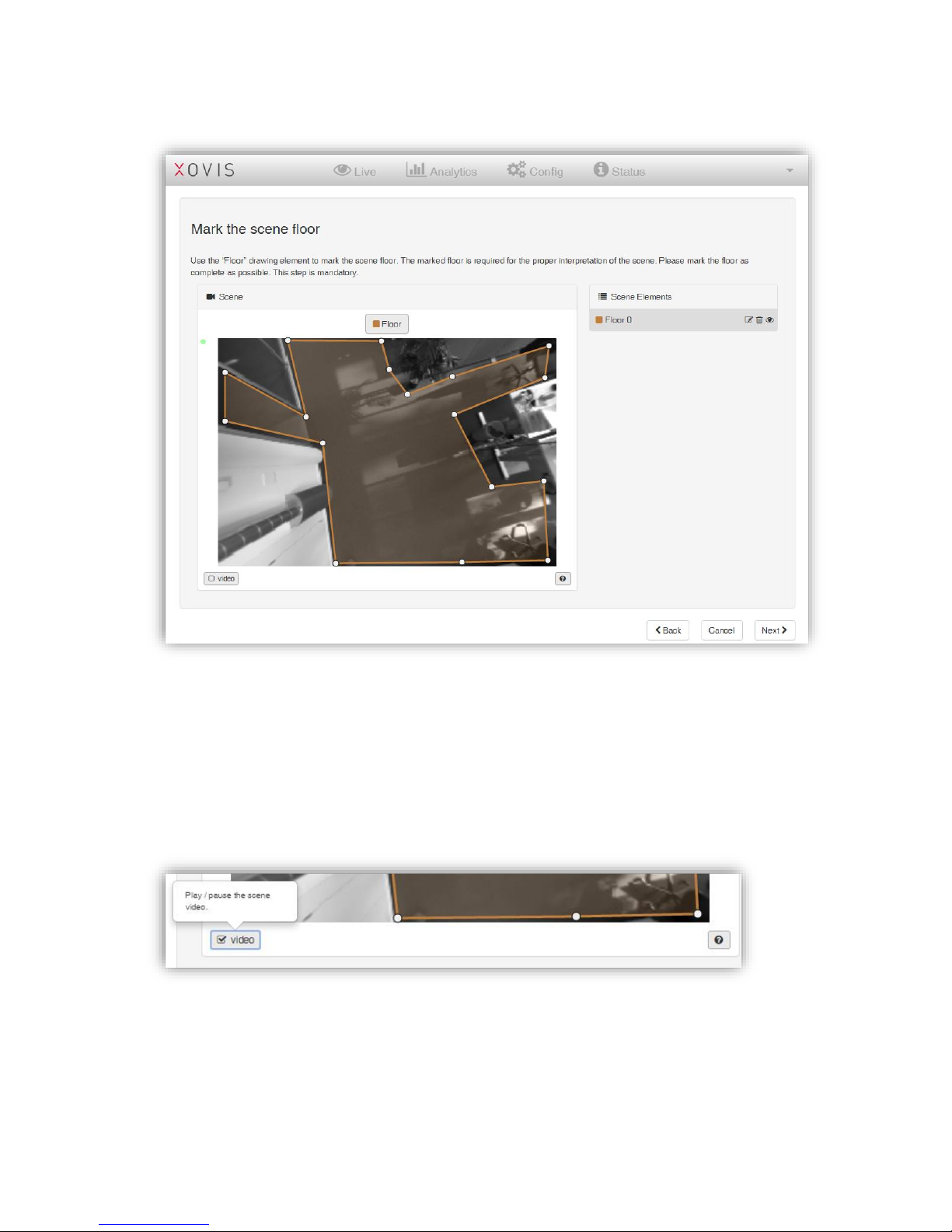
Figure 19: Drawn scene floor
In the next screen, the user is asked to mark the scene floor. The displayed scene image by
default is a still image as this usually simplifies the analysis of the scene environment.
However, if a video stream is preferred or maybe to just recapture a new still image, the live
stream can be displayed by clicking on the play button located below the scene image. The
help button beside the play button also offers a short explanation when hovering over it with
the mouse:
The floor is masked by selecting the drawing tool “Floor” and directly drawing the whole
floor as a polygon in the scene (see Figure 19). With the “Floor” tool activated, one can simply
click in the scene image to draw corners of a floor area. A floor area is finished by clicking on
the first corner again, by double-clicking to create the last corner, by disabling the “Floor”
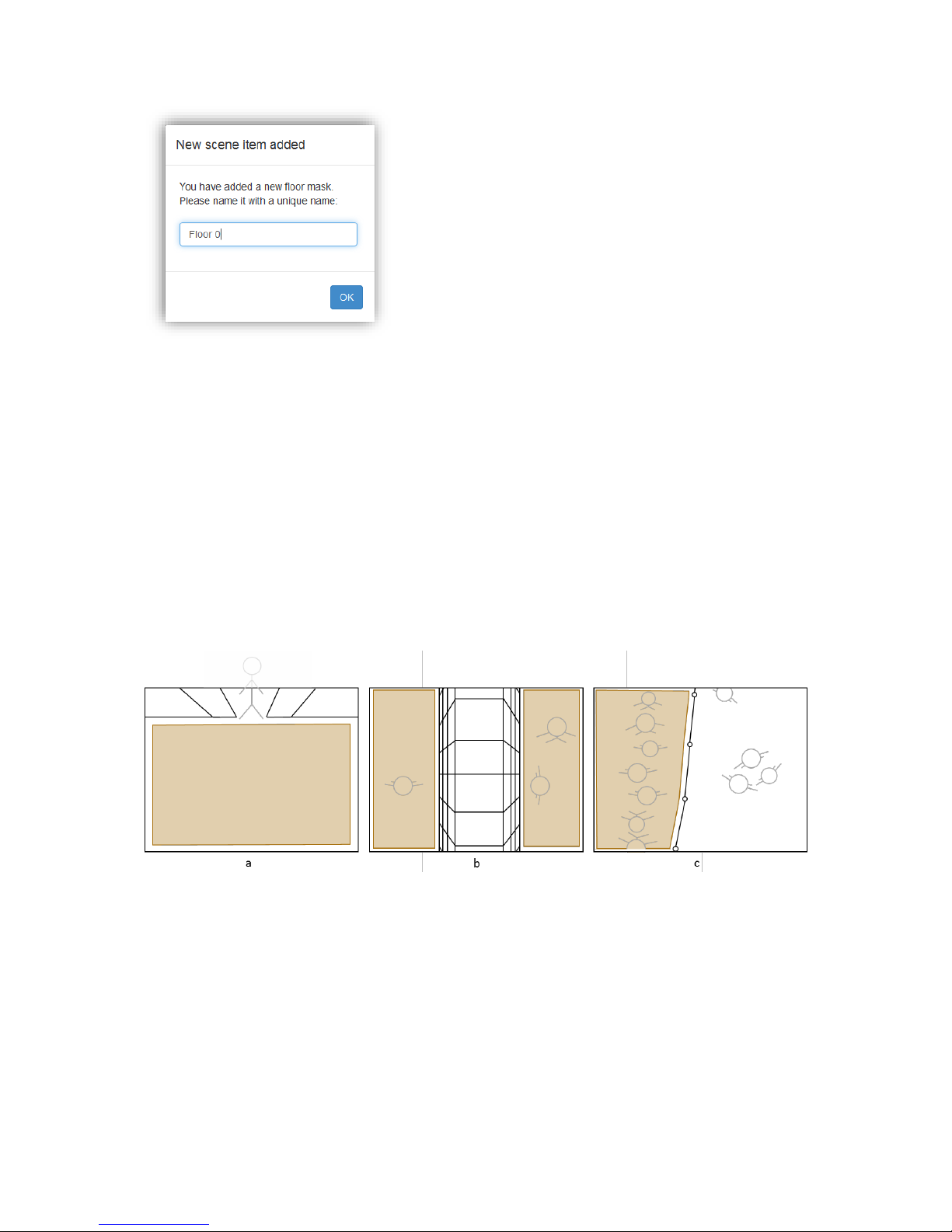
tool or by pressing [Esc] on the keyboard. After finishing a floor area, one is asked to name it
(see Figure 20). A default name is proposed.
Page 21
21 / 99 www.xovis.com
Figure 20: Name a scene item
As for all scene elements, this name must be unique among all other scene elements like
count lines and count zones. But at this point, the floor item will be the first scene item
added. After specifying a name, the floor is automatically added to the scene element list on
the right. There can also be more than one floor area (element) in the scene, e.g. for two
corridors covered by one sensor or just to simplify the drawing procedure for the user (see
Figure 21 b).
The floor mask defines the area in which persons should be detected by the sensor and
refers to the feet positions of a person. Usually the whole floor contained in a scene should
be covered by the floor mask. For special situations it can be desired to limit the floor mask
to a part of the actual floor only, e.g. when persons passing in a neighboring zone should be
ignored (see Figure 21 c).
Figure 21: Floor mask in different scene situations
As Figure 21 shows, it is a good practice to keep a small distance between the floor mask
and limiting objects like walls, doors or shelves. As mentioned already, it is also possible to
use more than one floor masks if the situation is demanding this.
To modify a floor mask the polygon points can simply be moved with the mouse. Doubleclicking on a polygon point will delete it, double-clicking on the polygon line will add an
additional point to the polygon. The whole polygon can be moved by clicking and holding the
mouse within the floor mask area and moving it to the desired location (drag-and-drop).
Page 22
22 / 99 www.xovis.com
The wizard requires the user to add at least one floor mask before continuing. However,
after finishing the wizard, the floor mask can theoretically be removed again. In that case,
if no floor mask is used, the whole scene is considered as floor and therefore enabled for
person detection.
The floor mask is applied when clicking “Next”.
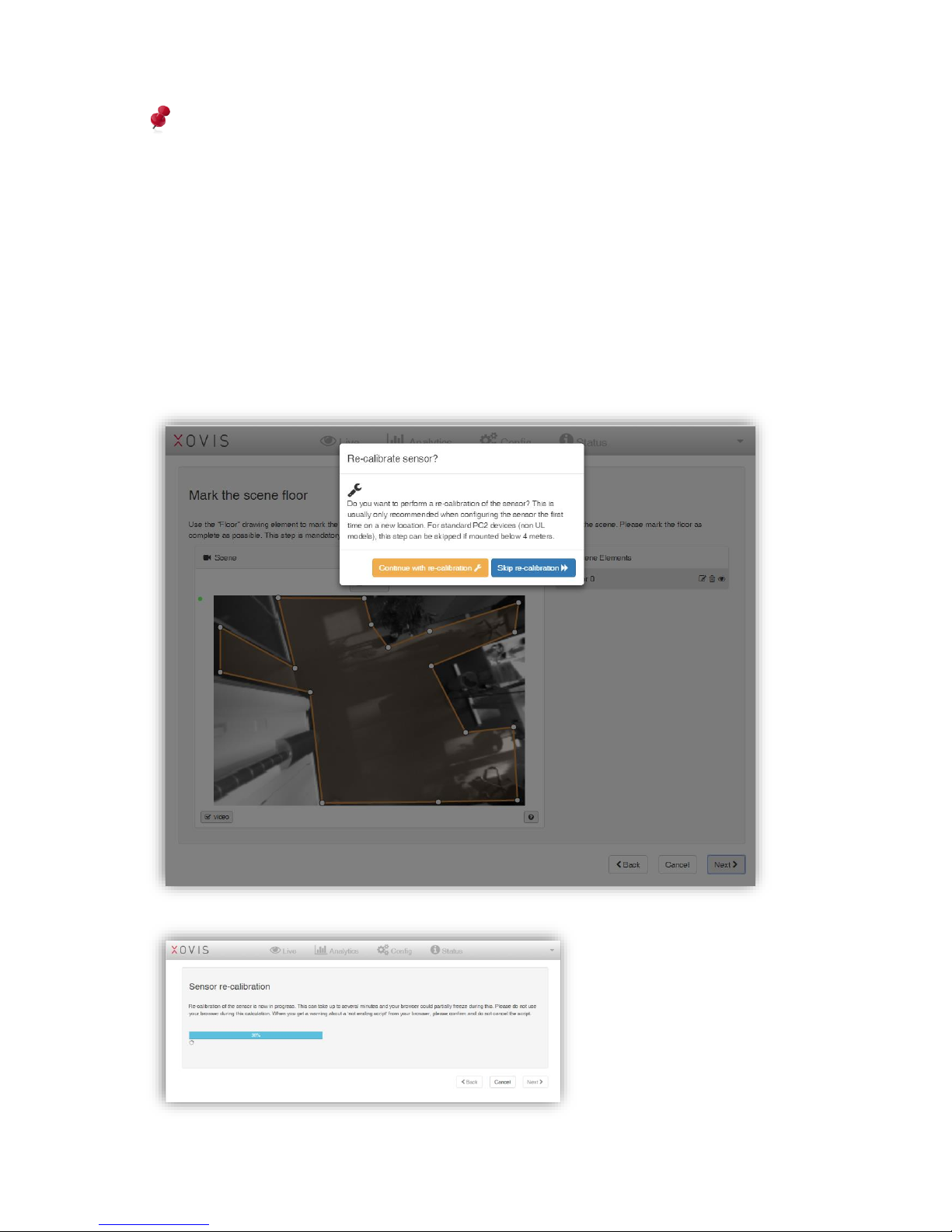
3.2.7.7 Re-calibrate Sensor
The wizard will now ask if a re-calibration should be applied. It is recommended to recalibrate the sensor when installing it for the first time in a new location. This step can be
skipped for standard PC2 devices being installed below 4 meters height and not in use in a
multisensor.
Page 23
23 / 99 www.xovis.com
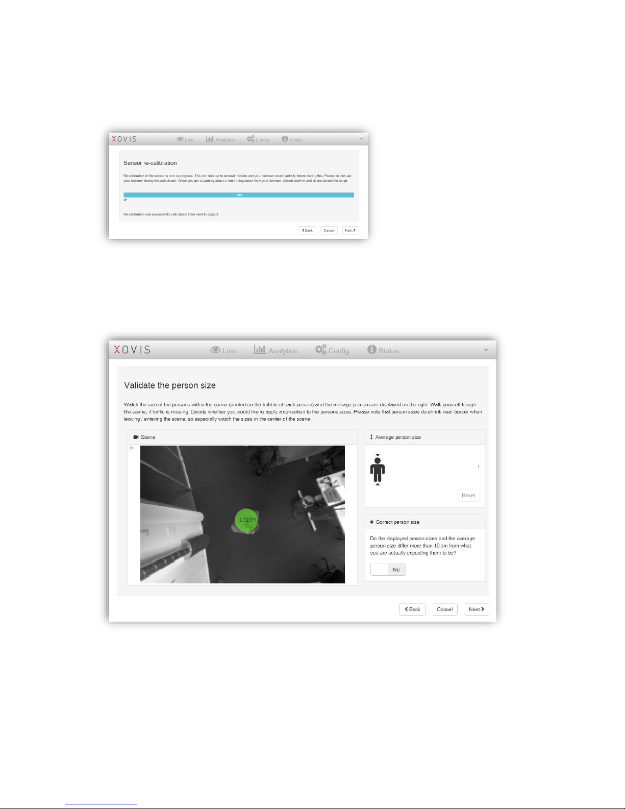
The recalibration requires a data exchange between the sensor and the web browser. If
performed by remote, the connection bandwidth will impact the duration and can take
several minutes. In such case we suggest a connection with at least 200kbytes/s.
When the re-calibration is done, it is applying to the sensors by clicking on “Next”.
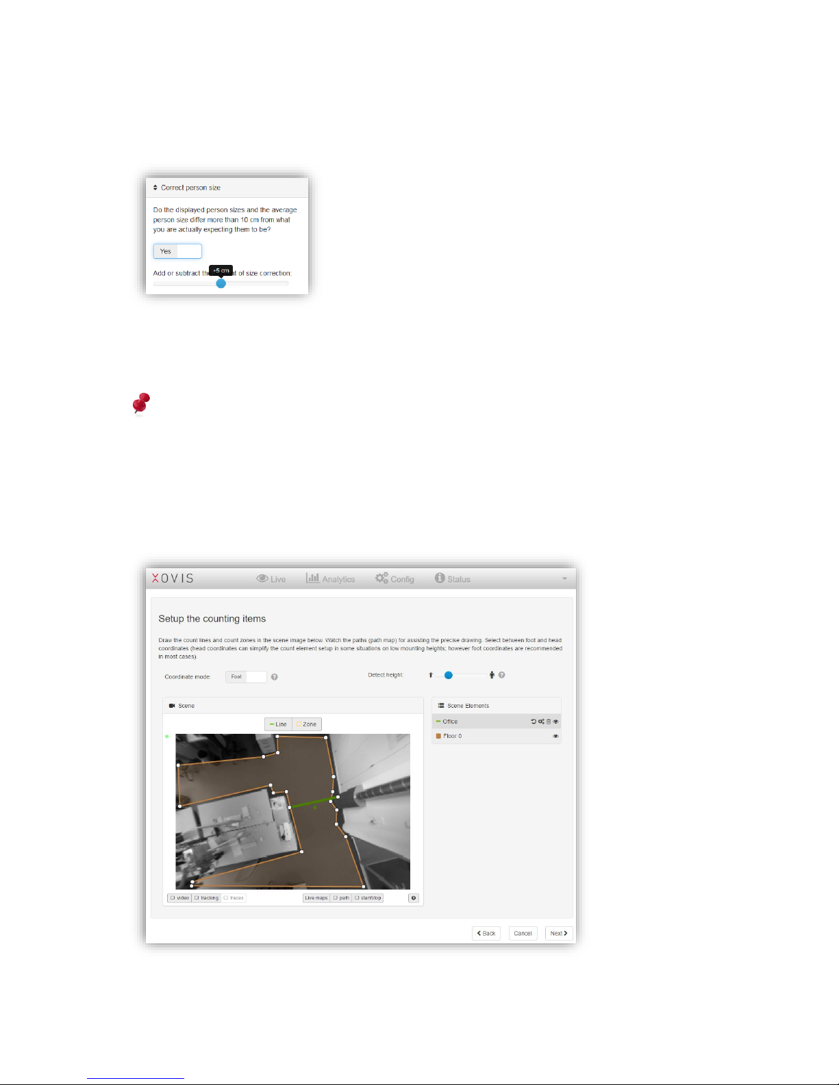
3.2.7.8 Validate the person size
In the succeeding screen, the user is asked to verify the person size. This is important to
validate the distance measurement of the sensor. In most cases, especially on mounting
heights below 3.5 meters, the person sizes will be quite exact without an additional
correction (precision is better than +/- 10 cm). But in several situations, the sensor might not
be able to correctly measure the scene and therefore measures the person sizes incorrectly.
If the average person size or the sizes printed on the bubbles within the scene seem to be
unrealistic, a correction can be applied. For this, the toggle switch in the “Correct person
172 cm
Page 24
24 / 99 www.xovis.com
size” box on the right must be set to “Yes”. Now, using the slider, a size correction can be
applied (the resolution is 5 centimeter based as this is the accuracy range the sensor is
operating).
When modifying the slider, the correction is automatically applied to the scene, so the effect
can be observed immediately. Also the average person size is reset every time the slider is
moved.
Please note that person sizes do shrink near border when leaving / entering the scene, so
especially watch the sizes in the center of the scene. The average person size uses the
maximum height of each person detected within the scene, so it is more representative.
After verifying the person sizes, any correction is applied to the sensor after clicking “Next”.
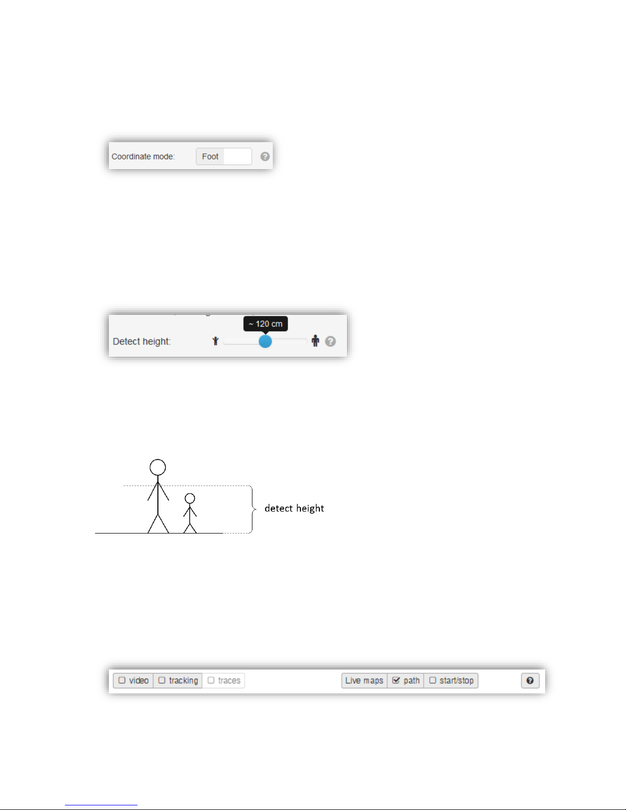
3.2.7.9 Setup the counting items
Page 25
25 / 99 www.xovis.com
In the next screen, the counting setup can be performed. In the upper part of the screen, the
coordinate mode and the detect height can be set.
3.2.7.9.1. Coordinate mode
The coordinate mode defines where to show the tracking of a person, either at its head or at
its feet. The purpose of the coordinate mode and the difference between “head” and “foot” is
explained in detail in chapter 3.1.2.
When toggling between the two coordinate modes, the sensor will automatically apply the
changed mode and switch the displaying of the person positions accordingly.
3.2.7.9.2. Detect height
The detect height defines the height from floor, at which a person gets detected and analyzed
by the sensor. This parameter influences the detection of small persons (children) and can
be reduced to 80 cm at least. With this parameter the exclusion from persons below a
specific size can be realized, i.e. to ignore children from being counted. The detect height can
be parameterized between 80 cm and 160 cm. Figure 22 visualizes the detect height.
Figure 22: Detect height
When changing the detect height with the slider, the changes will automatically be applied to
the sensor so they can immediately be verified in the scene view.
3.2.7.9.3. Scene view controls
The scene view offers several controls which can be helpful when setting up the counting
elements.
The first control, the video checkbox, allows to activate or de-activate the live video.
Page 26

26 / 99 www.xovis.com
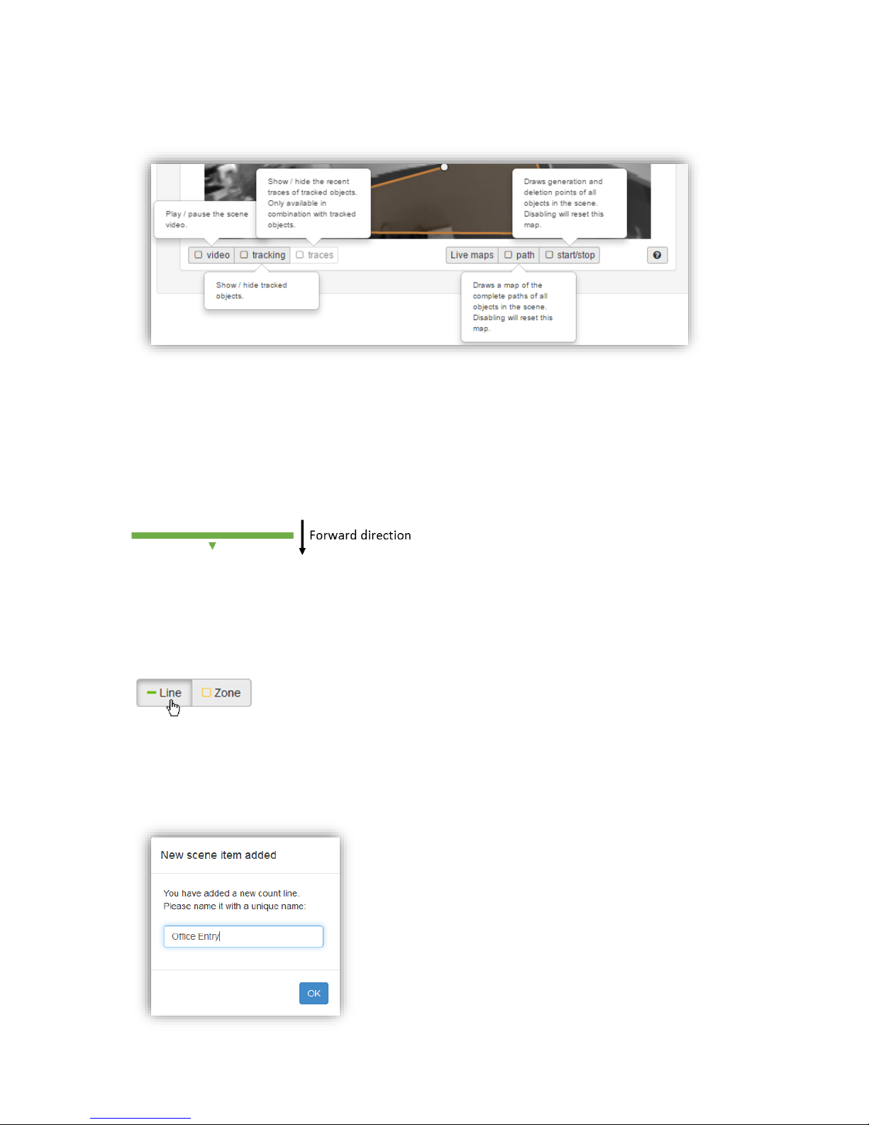
The “tracking” checkbox controls whether to show a bubble on every tracked person. This
bubble will be located either on the person’s head or feet, depending on the chosen
coordinate mode (see chapter 3.2.7.9.1).
Figure 23: Bubble displayed on tracked person
The “traces” checkbox is only activated when the “tracking” checkbox is selected. If “traces”
is selected, the most recent part of the track of every person within the scene is visualized:
Figure 24: Displayed path of tracked person
The “Live maps” section allows to show/hide several types of visualization maps: If the
“path” checkbox is selected, the whole tracks of all persons are kept and visualized in the
scene image. This path map can be of great use while drawing the counting elements
properly as the displayed paths help the user to identify the areas where tracking actually
occurs:
Figure 25: Pathmap helps to identify the actual tracking while setting up the counting elements
Page 27
27 / 99 www.xovis.com
Note: When the “path” checkbox gets unchecked, the tracks will disappear from the scene
view and be reset (when re-selecting the path live map checkbox, the old paths will not be
included again).
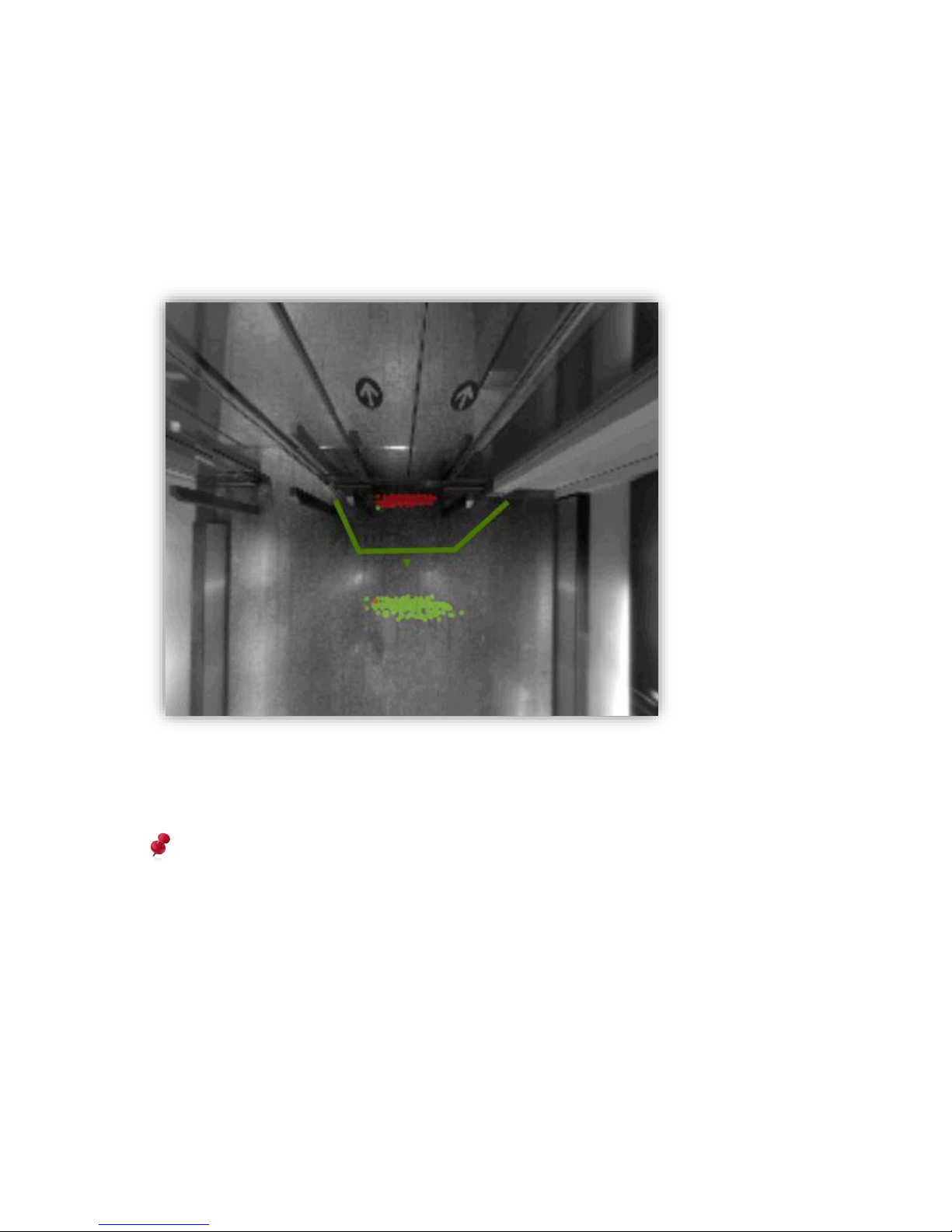
If the “start/stop” checkbox is selected, generation and deletion points of all persons will be
displayed as green and red dots. This allows to analyze, where people actually start to get
tracked and where they disappear again. Using this point map, a count line can be easily
adjusted properly to ensure to not miss any person.
Figure 26: Start/stop map visualizes generation and deletion points of persons
As with the path live map, when the “start/stop” checkbox gets unchecked, the points will
disappear from the scene and be reset.
Please note that all live visualizations are influenced by network bandwidth. As the
visualization are drawn by the client (web-browser) here, it is likely that some frames are
missed when low bandwidth is given. This leads to a visualization not showing the actual
truth, as, for example, start points will be drawn later as they actually occurred (location
will be more towards the inside of the scene).
Whenever using the maps for proper analytics, and especially with low bandwidth, it is
highly recommended to use the “visualization maps” instead, as they are based on
persisted, sensor-stored data. See chapter 3.2.9.2 for more details.
Page 28
28 / 99 www.xovis.com
The help button offers quick explanations for all the control elements mentioned so far.
Hovering over it with the mouse will pop-up the help information:
3.2.7.9.4. Count lines
The count line is the first of the two counting and observation tools available with a PCSeries sensor. A count line measures the number of persons crossing a defined line.
Forward and backward crossings are counted separately. A line therefore has a directional
property, i.e. an orientation. This orientation is indicated with a centered arrow pointing in
the direction of forward crossing (see Figure 27).
Figure 27: Orientation of a count line
A count line offers several ways to analyze person crossings for its counts. These strategies
are explained in section “Example Situations” in chapter 3.2.7.9.7 “Count line configuration”.
Drawing a count line
A line can be drawn by selecting the drawing tool “Line” and directly drawing the corners of
the line in the scene image. A line is finished with a second click on the last corner, by a
double click to create the last corner, by disabling the drawing tool “Line” or by pressing
[Esc] on the keyboard. After finishing a line, the user is asked to name it.
Page 29
29 / 99 www.xovis.com
As with the floor masks, this name must be unique among all other scene elements. After
naming the line it is automatically added to the scene element list.
In the examples shown above, a line always has two corners / points. However, a line can
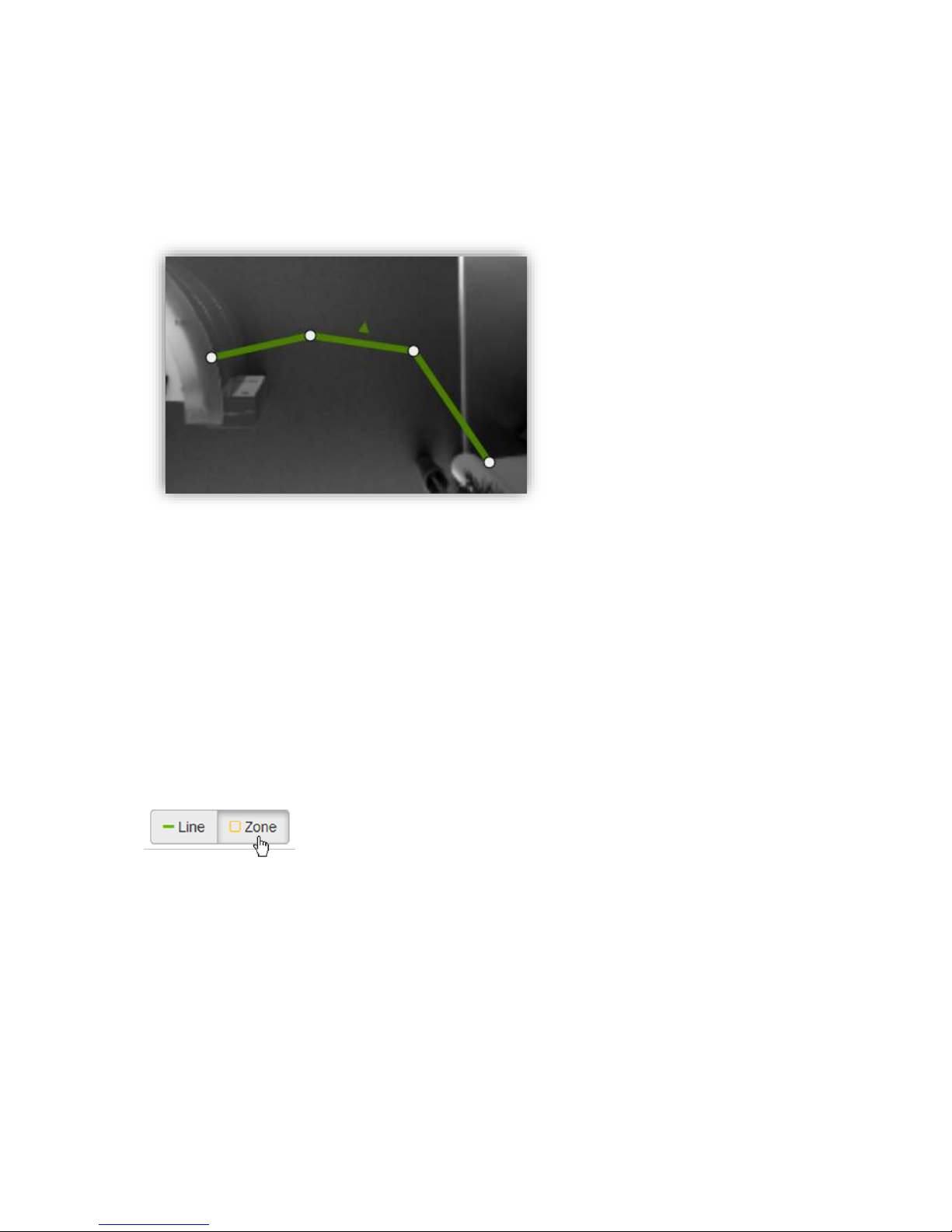
have multiple points (corners) to fit all situations. Such a multi-point line can be created by
just going ahead drawing corner points in the scene. Figure 28 shows an example:
Figure 28: A multi-point line
An existing line can be modified by moving its corners or by dragging the whole line by
clicking-and-holding on a line edge.
The sensor supports up to 8 count lines. When the 8th line is drawn, the line drawing tool gets
disabled. One or more lines then need to be deleted to re-enable the line drawing tool.
3.2.7.9.5. Count zone
The count zone is the second counting and observation tool available with the PC2. A count
zone measures the occupancy of a defined zone. Every count zone provides a count level
which indicates the number of persons currently situated within the zone.
Drawing a count zone
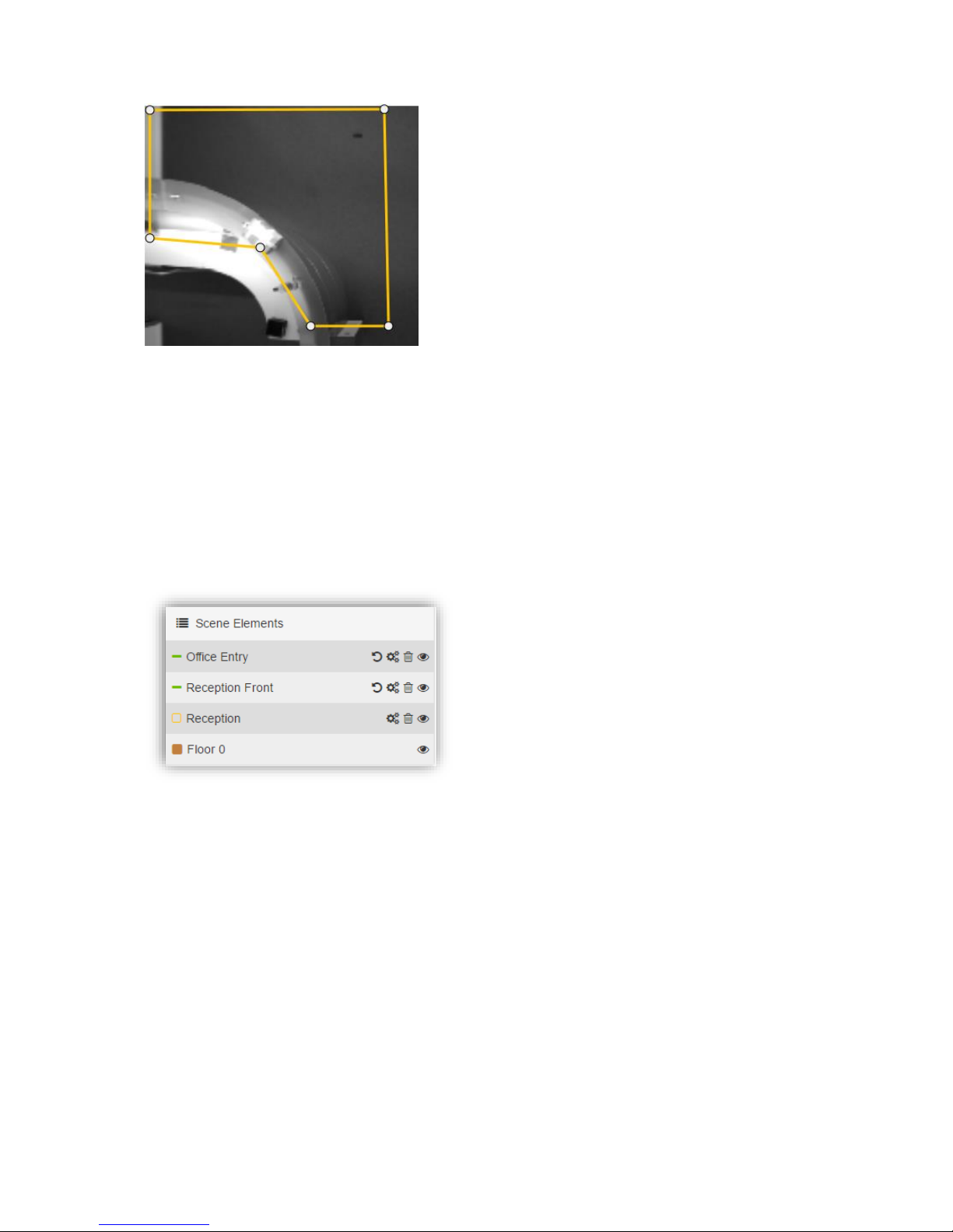
A count zone can be drawn similar to the floor mask. By selecting the drawing tool “Zone”
one can simply draw the corner points of the zone polygon in the scene image. A count zone
can be finished by clicking on the first corner again, by double-clicking to create the last
corner, by disabling the “Zone” tool or by pressing [Esc] on the keyboard. As with the count
lines, after finishing, the user is asked to name the count zone before it gets automatically
added to the scene element list.
Page 30
30 / 99 www.xovis.com
Figure 29: A count zone
Editing a count zone is the same as with the floor masks.
The sensor supports up to 8 count zones. When the 8th zone is drawn, the zone drawing tool
gets disabled. One or more count zones then need to be deleted to re-enable the zone
drawing tool.
3.2.7.9.6. Scene elements
All the scene elements described so far (floor masks, count lines, count zones) are listed in
the scene elements box:
Figure 30: Scene elements
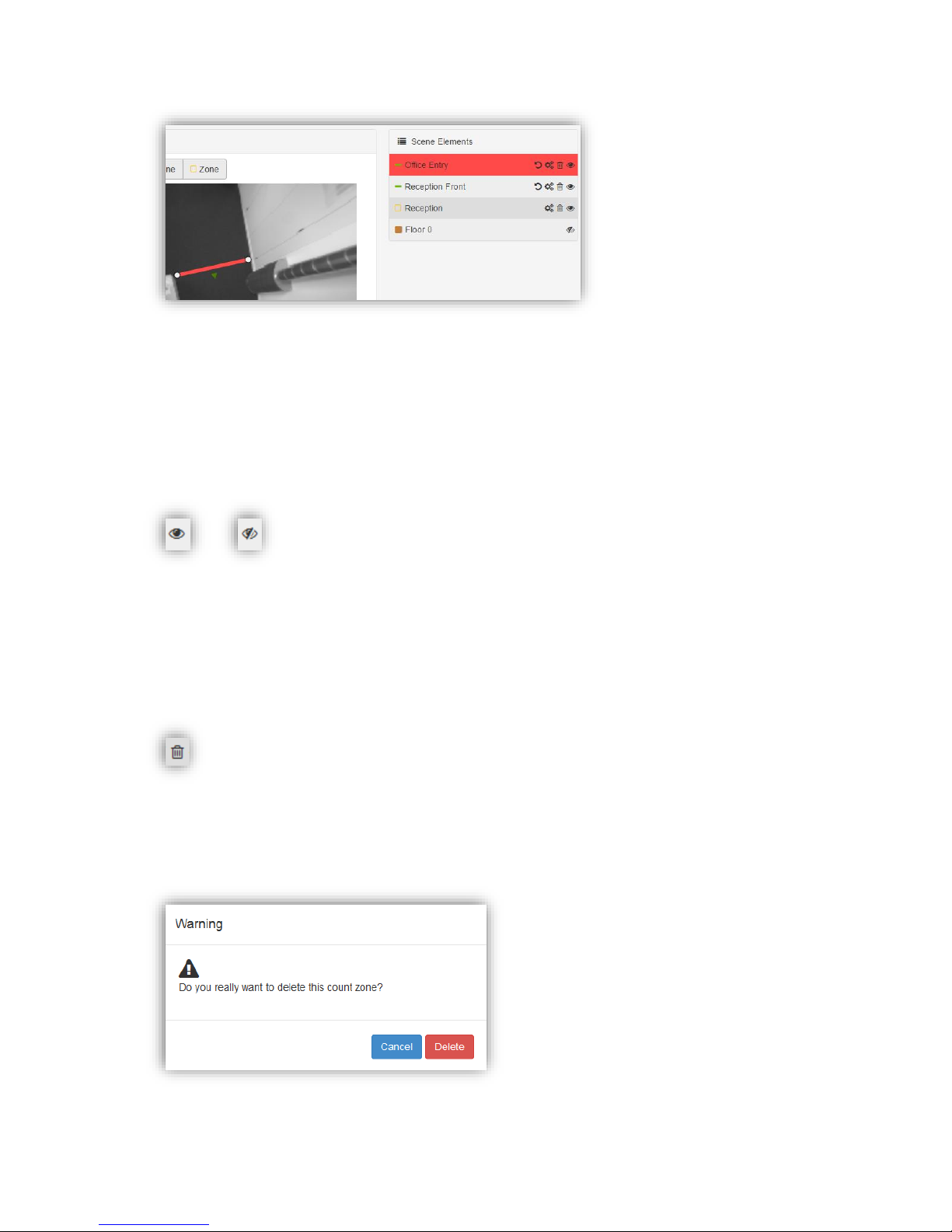
When hovering over the elements within the list, the element gets hightlighted both within
the list and within the scene. When clicking on a specific element, it gets marked red both
within the list and within the scene. At the same time the selected element is brought to the
front of the scene view, allowing to modify it even if it was actually lying behind another
element (e.g. count line behind a count zone). Clicking again on the element or selecting
another element will unmark it again. The vice-versa procedure is also supprted, i.e.
hovering and selecting the scene elements within the scene view. Figure 31 shows an
example:
Page 31
31 / 99 www.xovis.com
Figure 31: Highlighted scene element
Every scene element offers a series of icons on the right side of the list entry:
Show / hide a scene element
The eye icon allows to hide and show any scene element. This can be of use especially when
dealing with a certain amount of scene elements. As the floor mask usually covers a big part
of the scene image, it can be helpful to hide it when modifying other scene elements.
Figure 32: Hide / show a scene element
Delete a scene element
The trash bin icon allows to delete any scene element. During the wizard, the floor mask,
once set, cannot be deleted as it is mandatory. However, after finishing the wizard, even the
floor masks can be deleted the same way as any other scene element.
Figure 33: Delete a scene element
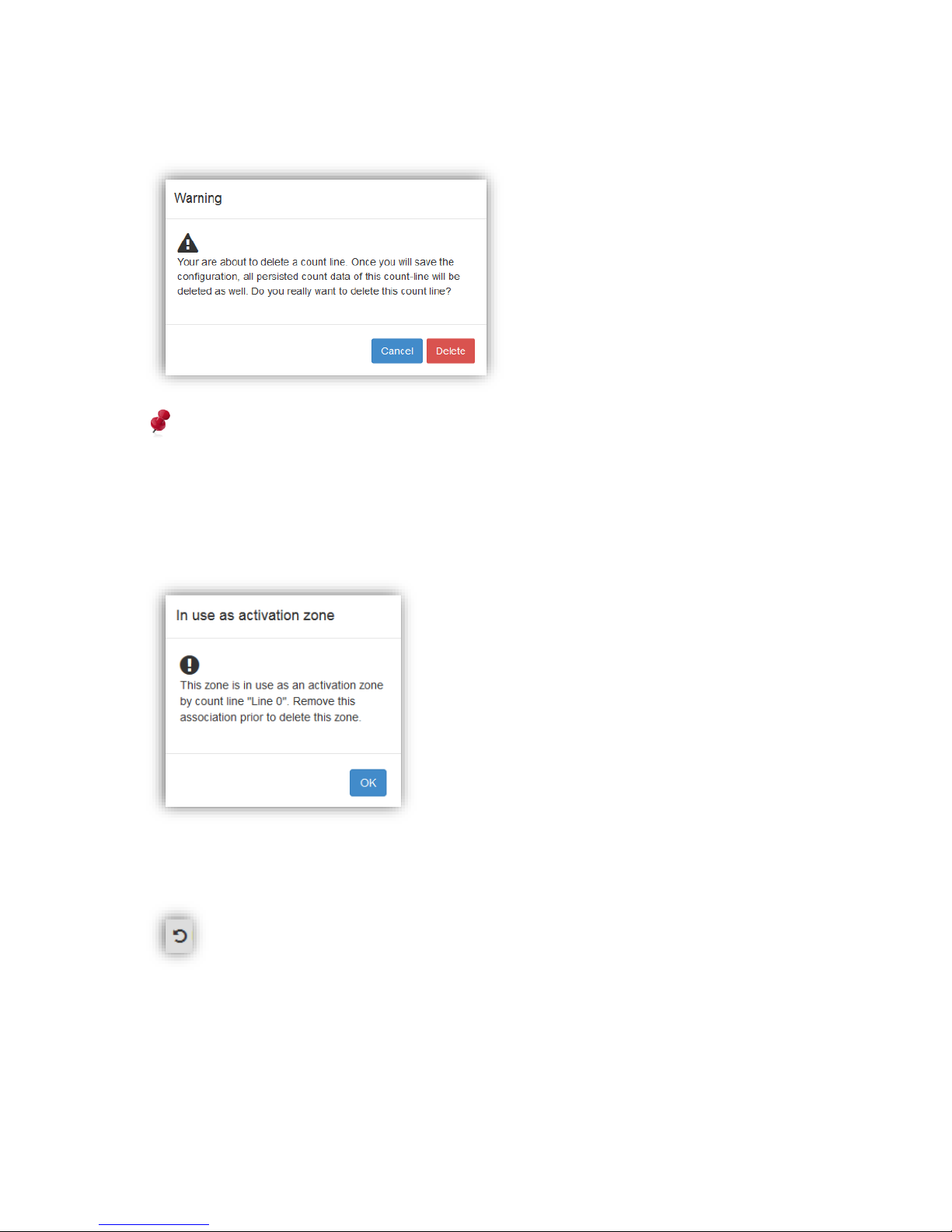
When clicking on the trash bin icon, the user is asked to confirm the deletion of the specific
scene element:
Page 32
32 / 99 www.xovis.com
When deleting a count line, a special warning will inform the user that all persisted count
data belonging to this count line will be deleted as well:
Attention: When deleting a count line, all persisted count data of this count line will also be
deleted!
When trying to delete a count zone which is in use as an activation or deactivation zone (more
on this later), a special warning will inform the user that the association has to be removed
prior to be able to delete the count zone:
Switch count line orientation
The count lines offer an additional icon within the scene element list, the rotate icon:
Figure 34: Switch count line orientation
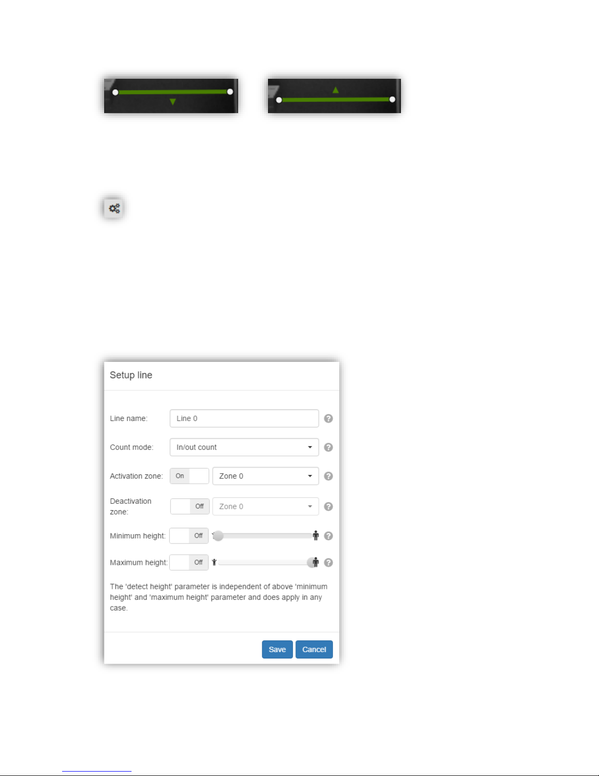
When clicking on this icon, the specific count line switches its orientation. Thereby the arrow
indicating the lines forward direction will appear on the other side of the line, indicating that
the counting direction changed:
Page 33
33 / 99 www.xovis.com
Count item configuration
The count lines and count zones offer an additional icon within the scene element list, the
gear-wheel icon:
Figure 35: Open count item configuration
When clicking on this icon, a dialog is displayed allowing the user to control a series of
parameters associated with this count item. These parameters are explained in the following
two chapters, Count line configuration and Count zone configuration.
3.2.7.9.7. Count line configuration
The count line configuration displays the following dialog:
Figure 36: Count line configuration
Page 34
34 / 99 www.xovis.com
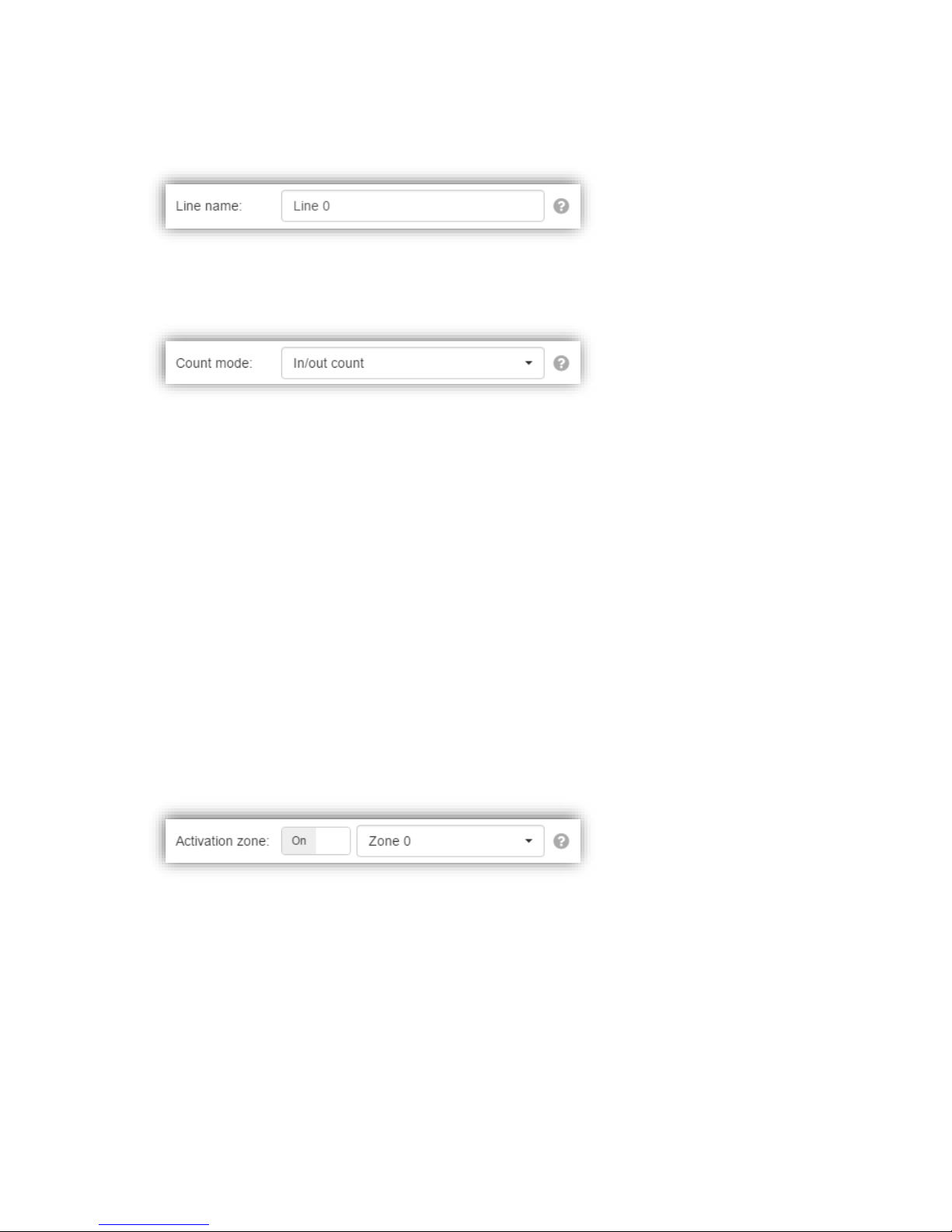
Line name
The first text field allows to change the name of the count line:
Count Mode
The dropdown menu located just below, allows to specify the count mode of this count line:
The count mode defines the strategy how line crossings of a person shall be processed. Two
different count modes are available:
In/out count: The first crossing of a person is updated immediately. When the person
exits where entered, this count will be updated as well as soon the person gets
deleted. This mode is activated by default.
Late count: Every person’s line crossings are first evaluated and counted when he
leaves the scene. Forward and backward counts of a single person on the same line
thereby cancel out each other. That way, multiple counting of one and the same
person which moves continuously forward and backward in the region of the count
line is ignored. This is the preferred mode to get exact counting per person with the
limitation of possible delayed counter updates due to the fact that the counters are
first updated when a person leaves the scene.
Activation zone
The activation zone toggle allows to enable the use of any zone as an activation zone for this
count line:
If toggled to “On”, the dropdown allows to define any of the configured count zones as an
“activation zone”. Whenever an activation zone is associated to a count line, person crossings
are only counted on this count line when the person is either generated or deleted within the
activation zone.
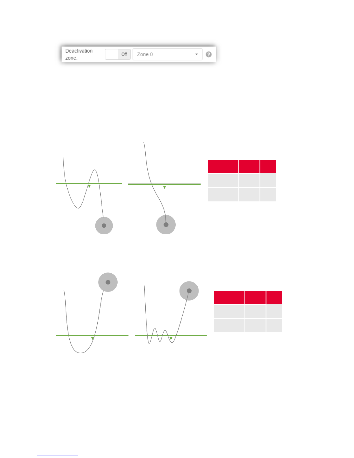
Deactivation zone
The deactivation zone toggle allows to enable the use of any zone as a deactivation zone for
this count line:
Page 35
35 / 99 www.xovis.com
The deactivation is the opposite to an activation zone. If toggled to “On”, the dropdown allows
to define any of the configured count zones as a “deactivation zone”. Whenever a deactivation
zone is associated to a count line, person crossings are only counted on this count line when
the person is neither generated nor deleted within the deactivation zone.
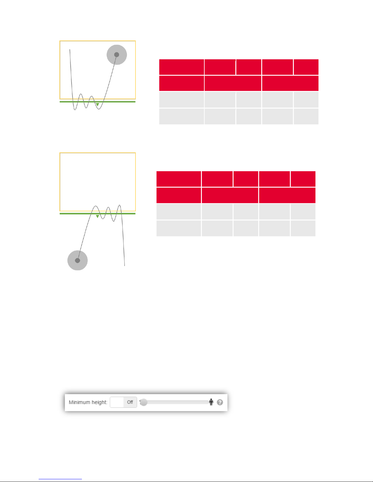
Example situations
In the following, several examples demonstrate the difference between the two count modes
and the effect of an associated activation/deactivation zone:
Counts
In/out
Late
Forward
1 1 Backward
0
0
Figure 37: Count mode example 1
Counts
In/out
Late
Forward
1
0
Backward
1
0
Figure 38: Count mode example 2
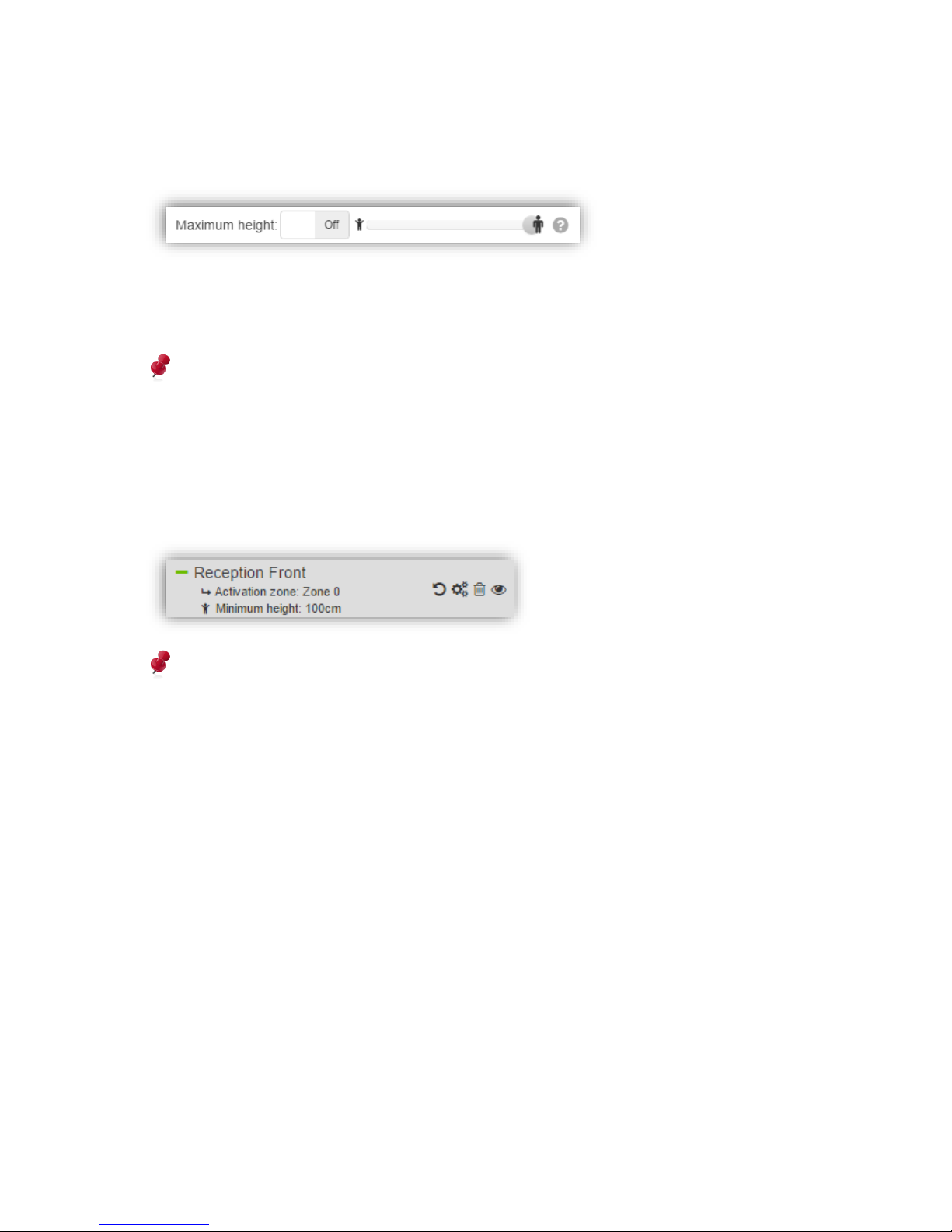
Page 36
36 / 99 www.xovis.com
Counts
In/out
Late
In/out
Late
Activation Zone
Deactivation Zone
Forward
1 0 0
0
Backward
1 0 0
0
Figure 39: Count mode example 3
Counts
In/out
Late
In/out
Late
Activation Zone
Deactivation Zone
Forward
0 0 1
0
Backward
0 0 1
0
Figure 40: Count mode example 4
The examples show that the chosen counting mode as well as the use of an
activation/deactivation zone can be crucial to the desired behavior. “In/out count” is
recommended count mode as it combines instantaneous update of the first crossing plus
filtering of person wobbling on the line.
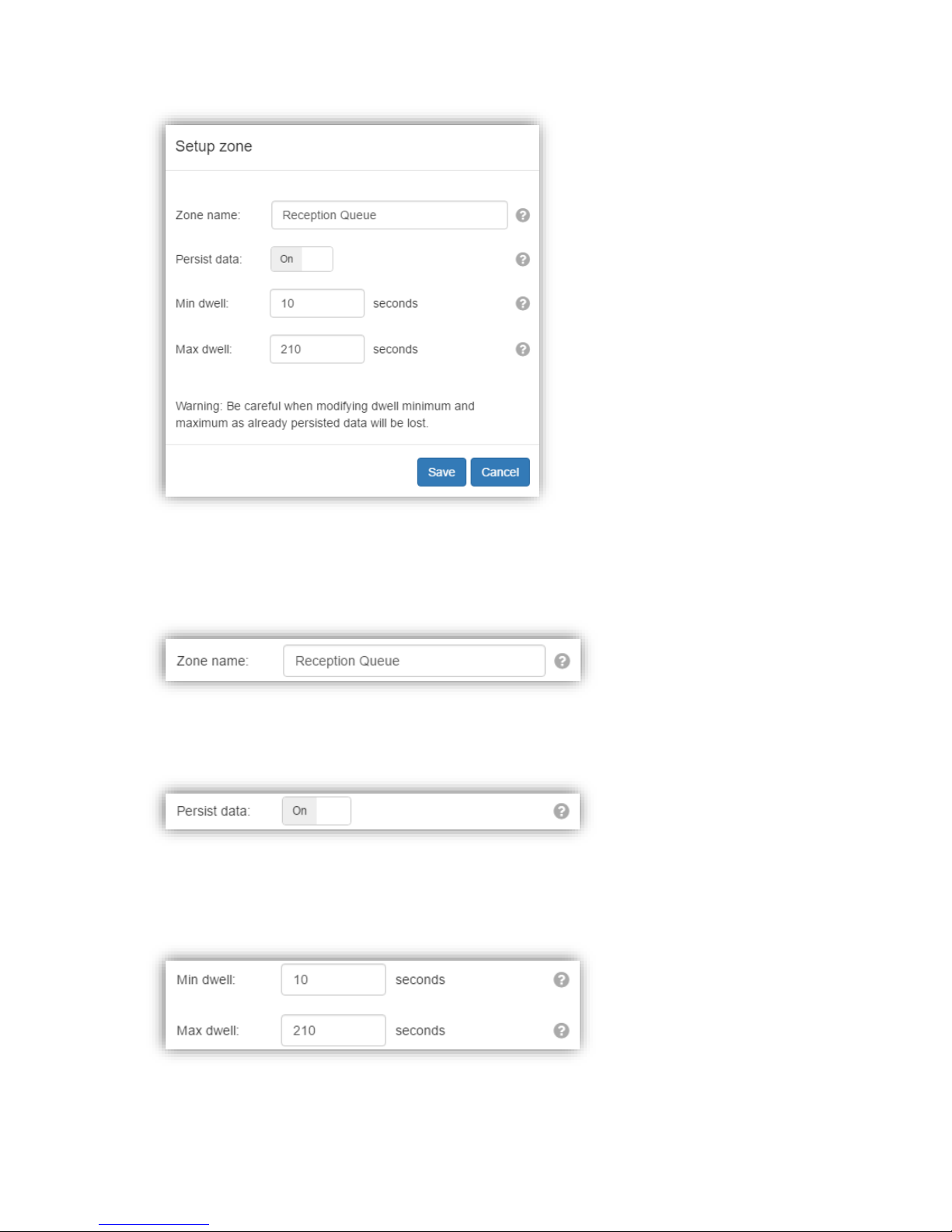
Minimum height
The minimum height toggle allows to enable a specific minimal height of persons considered
for counting:
All persons showing a height smaller than this defined minimum height will not lead to a
count on this count line. This can for example be of use for excluding children to be counted.
Page 37
37 / 99 www.xovis.com
Maximum height
The maximum height toggle allows to enable a specific maximal height of persons
considered for counting:
All persons showing a height taller than this defined maximum height will not lead to a count
on this count line. This can for example be of use for only counting children on this count
line.
For counting children and adults separately at the same location, two individual count
lines can be drawn, one with a minimum height rule applied, the other with a maximum
height rule applied.
Specific settings of a count line are directly displayed in the scene item list. The example
below indicates that “Zone 0” is set as activation zone and that persons below 100 cm height
are not considered for counting for this count line:
Please be aware, that some of the above count line settings require a delayed evaluation
of person tracks. Counts can therefore first show up after the deletion of a person,
independent of the count mode. For example, when specifying a minimum height on a
count line, the average height of all crossings of a person is used for evaluating the
criterion. Therefore the counting can fist be done when a person gets deleted.
3.2.7.9.8. Count zone configuration
The count zone configuration displays the following dialog:
Page 38
38 / 99 www.xovis.com
Figure 41: Count zone configuration
Zone name
The first text field allows to change the name of the count zone:
Zone data persistence & dwell time
If toggled to “On”, fill level and dwell time statistics are stored on the sensor:
When set to “On”, a minimum and a maximum dwell time have to be specified. Persons
dwelling for a shorter time than the minimum dwell time set here are not considered for
dwell time statistics. Same with the maximum dwell time.
Page 39
39 / 99 www.xovis.com
The time span between the minimum and maximum dwell time is divided into 10 bins of
equal size for dwell time distribution. See also chapter 3.2.9.1.1 “Count zone charts” for
more details on this.
For meaningful dwell time statistics, it is important to place the zone correctly inside the
sensor actual tracking area. Only tracks started and ended outside the zone are
considered for dwell time calculation. Please refer to chapter 4.3 “Placement of dwell
zones” for more information on this.
3.2.7.10 Privacy mode
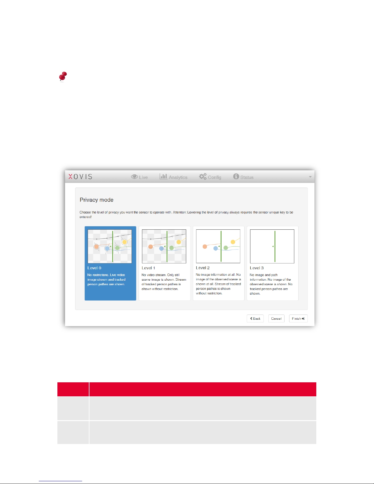
After setting up the counting items, the next screen allows to define the privacy mode. The
sensor offers 4 level of privacy:
Level
0
No restrictions. Live video of the scene as well as tracking is shown without any
restrictions.
1
Only a still image of the scene is shown, no video stream. This still image can
be refreshed on request. Tracking is shown without restrictions.
Page 40

40 / 99 www.xovis.com
2
No image information is shown at all. The scene background is just displayed
as a white area. Tracking is shown without restrictions.
3
No image information and no tracking information is shown. Only the counting
values are updated.
Page 41
41 / 99 www.xovis.com
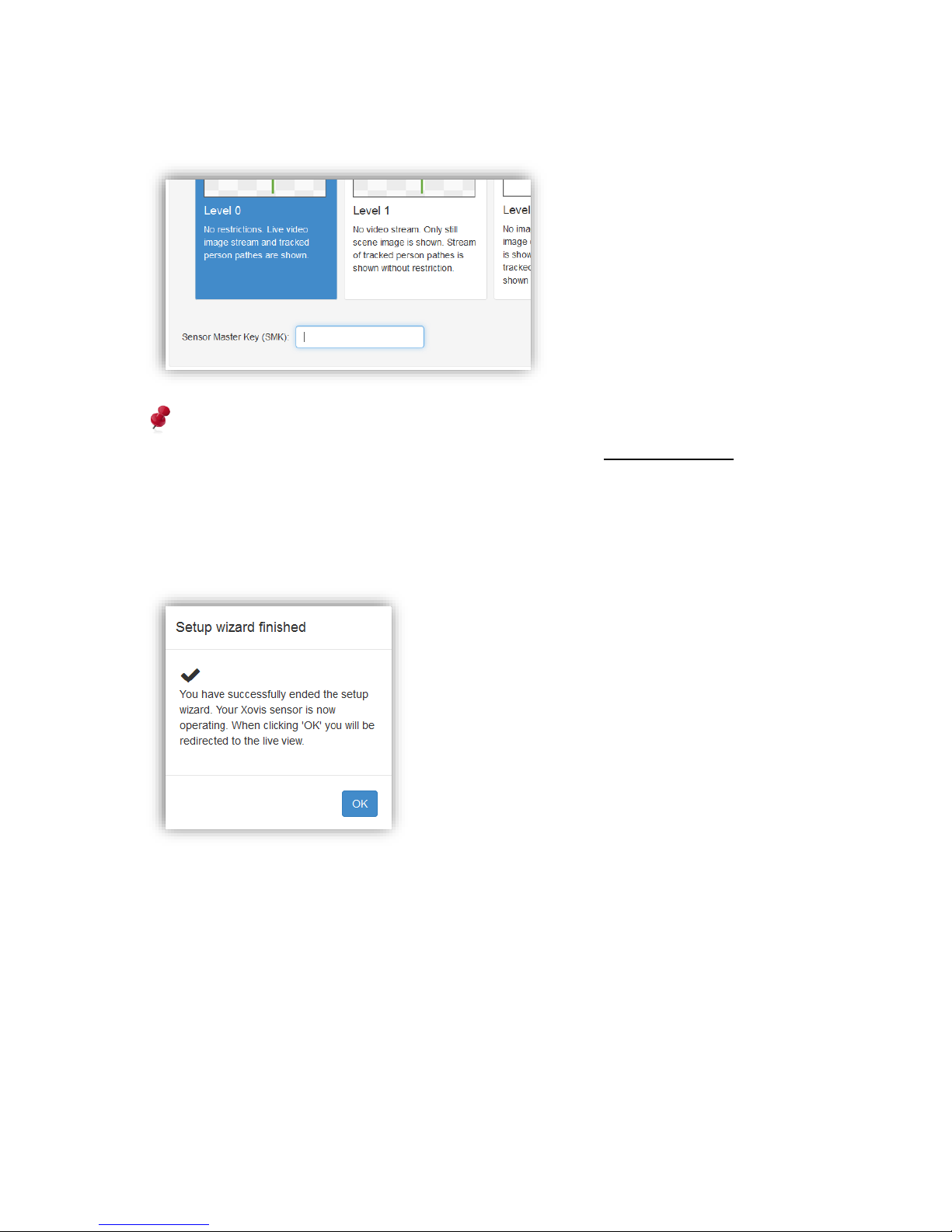
Increasing the privacy mode to a higher level can always be done. However, when lowering
the privacy mode, the Sensor Master Key (SMK) has to be specified:
The Sensor Master Key is unique for every sensor and is provided together with the
corresponding order invoice. Alternatively send a request to [email protected]
3.2.7.11 Finishing the wizard
When the privacy mode is set, the wizard will be finished by clicking on “Finish”. After
applying all settings to the sensor, the wizard will end with the following message:
After clicking “OK”, the wizard will be closed and the user is redirected to the live view.
Page 42
42 / 99 www.xovis.com
3.2.8 Live View
The live view is the default landing page after logging in to the sensor or after finishing the
setup wizard.
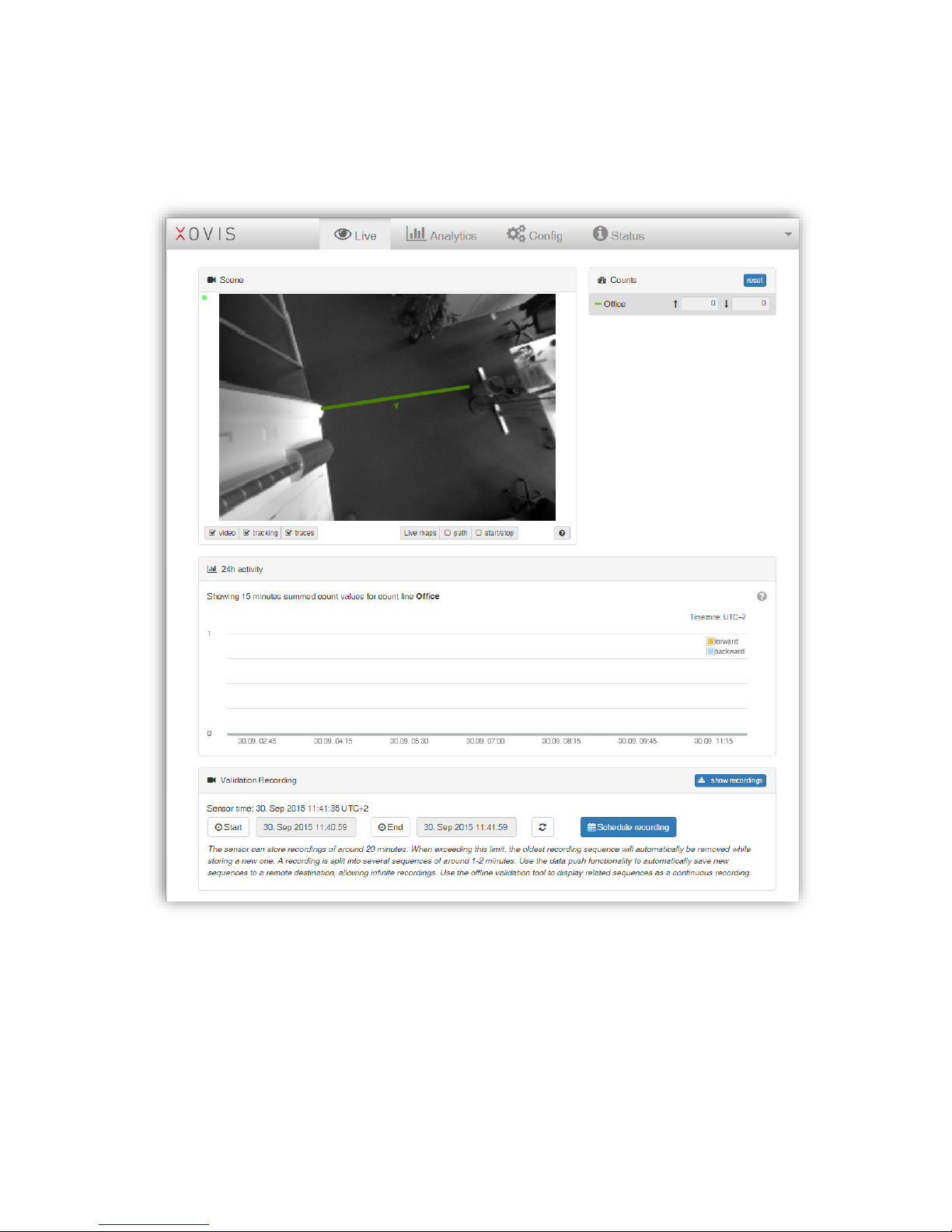
Figure 42: Live view
Page 43
43 / 99 www.xovis.com
The live view holds four main parts:
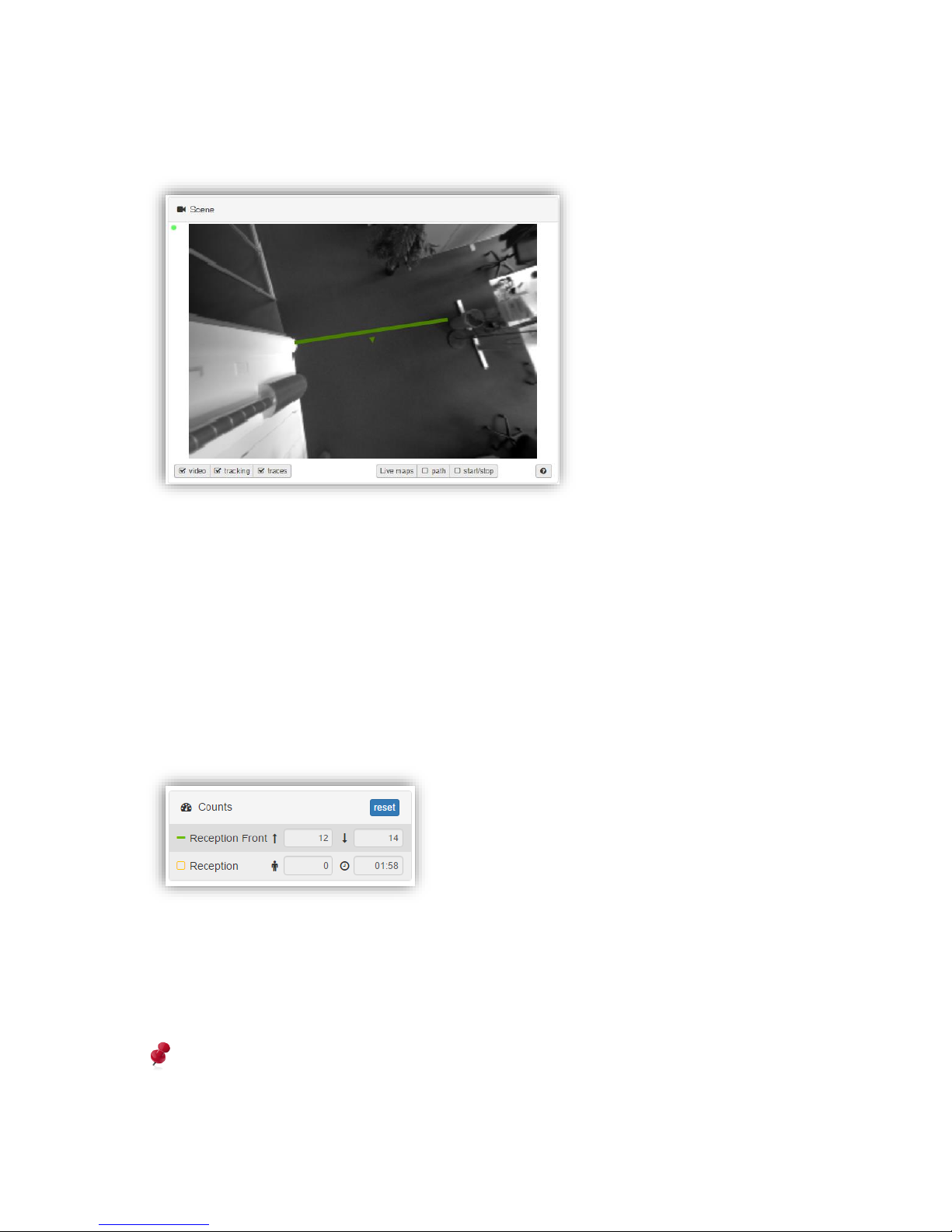
3.2.8.1 Scene live view
The “Scene” box holds the live view of the sensors scene. Configured count lines and count
zones are overlaid in the scene image. The monitoring can be controlled by the scene view
controls described in chapter 3.2.7.9.3.
When hovering over the count elements within the scene, the element gets hightlighted both
within the scene and within the “counts” list (mentioned in the next chapter). When clicking
on a specific element, it gets marked red both within the scene and within the “counts” list.
The blinking small green dot displayed in the upper left corner of the “Scene” box indicates
an intact connection to the sensor.
3.2.8.2 Live count states
The “Counts” box lists all configured count elements on the sensor, i.e. count lines and count
zones. For each count line the current values of their forward and backward counts are
displayed beside the count line name. For every count zone, the current person occupancy
i.e. the number of persons currently located within the zone as well as the average dwelling
time of the last 15 minutes is shown. The displayed values are updated every 3 seconds.
If no valid dwell times of a zone have been measured in the past 15 minutes, the dwell
time of a count zone will be displayed as “n/a” (not available).
Page 44
44 / 99 www.xovis.com
When hovering over the count elements within the list, the element gets hightlighted both
within the list and within the scene. When clicking on a specific element, it gets marked red
both within the list and within the scene.
The count values of the count lines can be reset to 0 by clicking on the small blue “reset”
button located in the header of the “Counts” box. Resetting the count values can be of use to
do a measurement starting at a specific point in time.
Resetting the count values can influence additional software that depends on the sensors
count data. However, as the sensor stores the count line values every minute, the stored
statistics will only be influenced for the last single minute.
3.2.8.3 24h live statistics
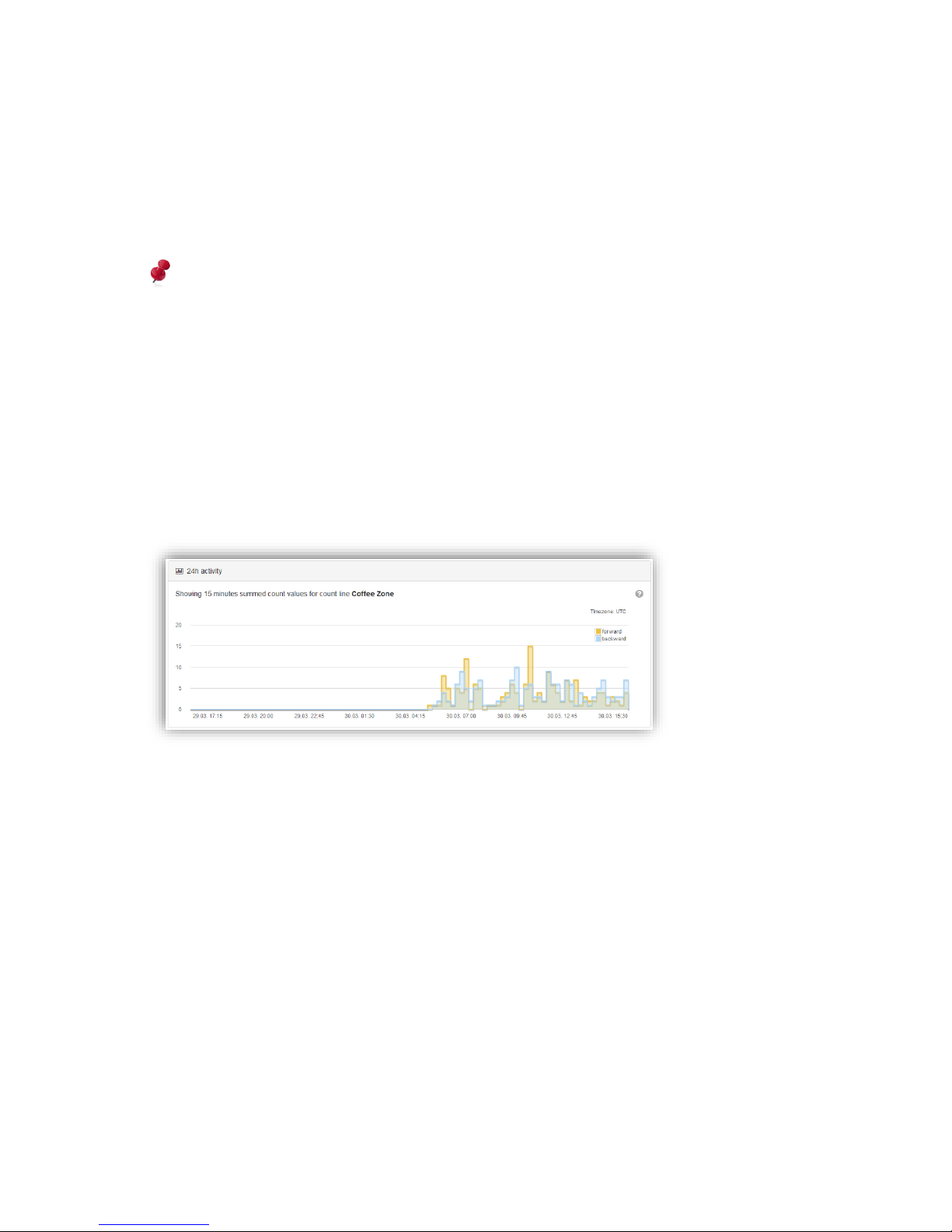
The 24h activity shows measurements of a specific count item of the past day. Per default,
the chart shows data for the top most count item (if at least one if defined). When clicking on
a count item, be it a line or a zone, the chart will display the corresponding data.
For count lines, both, the forward and the backward counts are displayed within the chart.
The values are summed up to 15 minute bins.
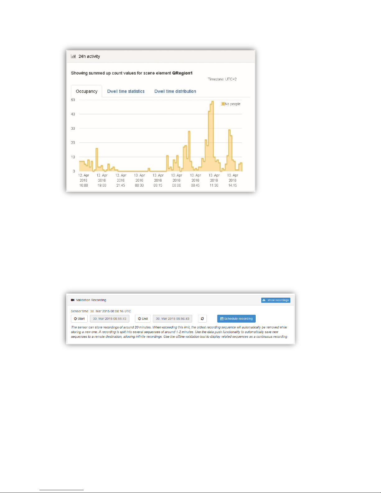
For count zones, in case the data persistence feature has been activated (see 3.2.7.9.8), the
occupancy as well as dwell times are available. The individual charts for occupancy, dwell
time statistics and dwell time distribution are accessible by selecting the respective tab:
Page 45
45 / 99 www.xovis.com
Occupancy and dwell time statistics represent the values in 15 minute bins. Dwell time
distribution shows a histogram of 10 bins with equal size, holding the values of the past 24
hours.
Refer to chapter 3.2.9.1.1 “Count zone charts” for more information on the persisted zone
data.
The chart is automatically updated every minute.
3.2.8.4 Validation Recording
The “Validation Recording” box allows to manage validation recordings of the sensor. A
validation recording contains the scene video, the person tracks, the count item
configuration and all line counting and crossing events. With these information, the sensors
functionality can easily be validated. Xovis provides the “Xovis Validation Viewer” tool to
analyze validation recordings offline.
The recordings are split into several sequences of 5MB. Use the Xovis Validation Viewer to
visualize the sequences belonging together (it can be downloaded from the Xovis Customer
Portal).
Page 46
46 / 99 www.xovis.com
3.2.8.4.1. Schedule a recording
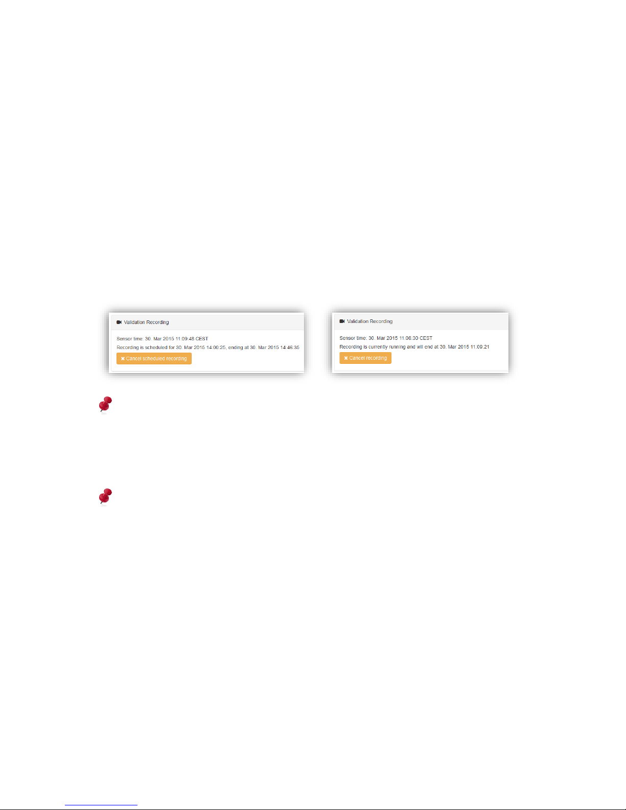
With the two date fields “Start” and “End”, a validation recording can be scheduled to a
specific period, starting now or in the future. When clicking “Schedule recording”, the
scheduling is stored. As soon the start time of the scheduling is reached, the sensor will
start to record the validation data. The recording is automatically stopped when reaching the
end time.
As the scheduling is always based on the sensors time which does not need to be the same
as the local time of the user’s computer currently configuring the sensor, the sensors time is
shown directly above the schedule items and is automatically refreshed periodically. By
clicking the “refresh”-icon (arrows in a circle) the scheduling start time is immediately
updated to the latest sensor time and the end time will hold the start time value plus 1
minute. This can be helpful to quickly start a short validation recording, i.e. if an interesting
situation seems to happen right that moment.
Whenever a recording is scheduled or running, the state is presented accordingly:
The sensor can store recordings of around 40 minutes. When exceeding this limit, the
oldest recording sequence will automatically be removed while storing a new one. A
recording is split into several sequences of 5MB. Using the data push functionality,
recorded sequences can be stored on a remote destination (FTP) allowing recordings of
any length.
A configuration change of any count line will not stop a pre-scheduled validation
recording, even though it is already ongoing. By saving a new configuration the sensor
stops a currently running recording and starts a new one immediately after completion of
the saving process.
Page 47
47 / 99 www.xovis.com
3.2.8.4.2. Manage recordings
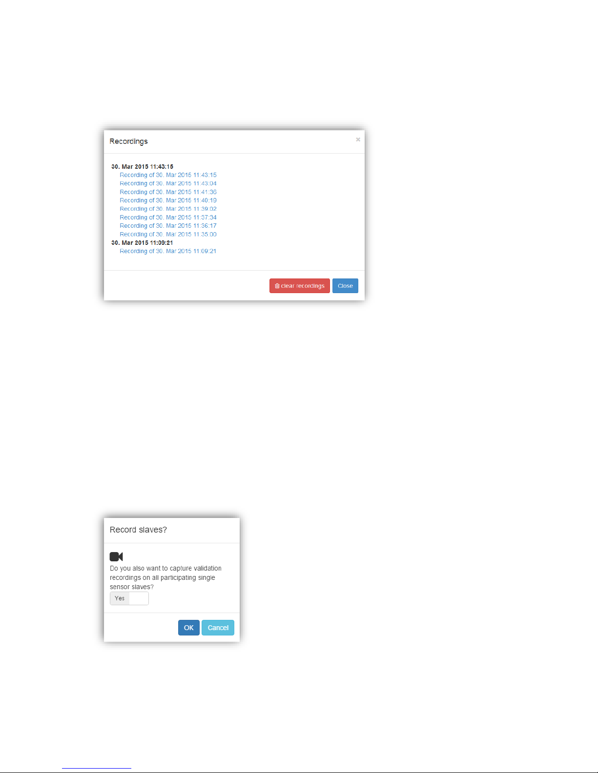
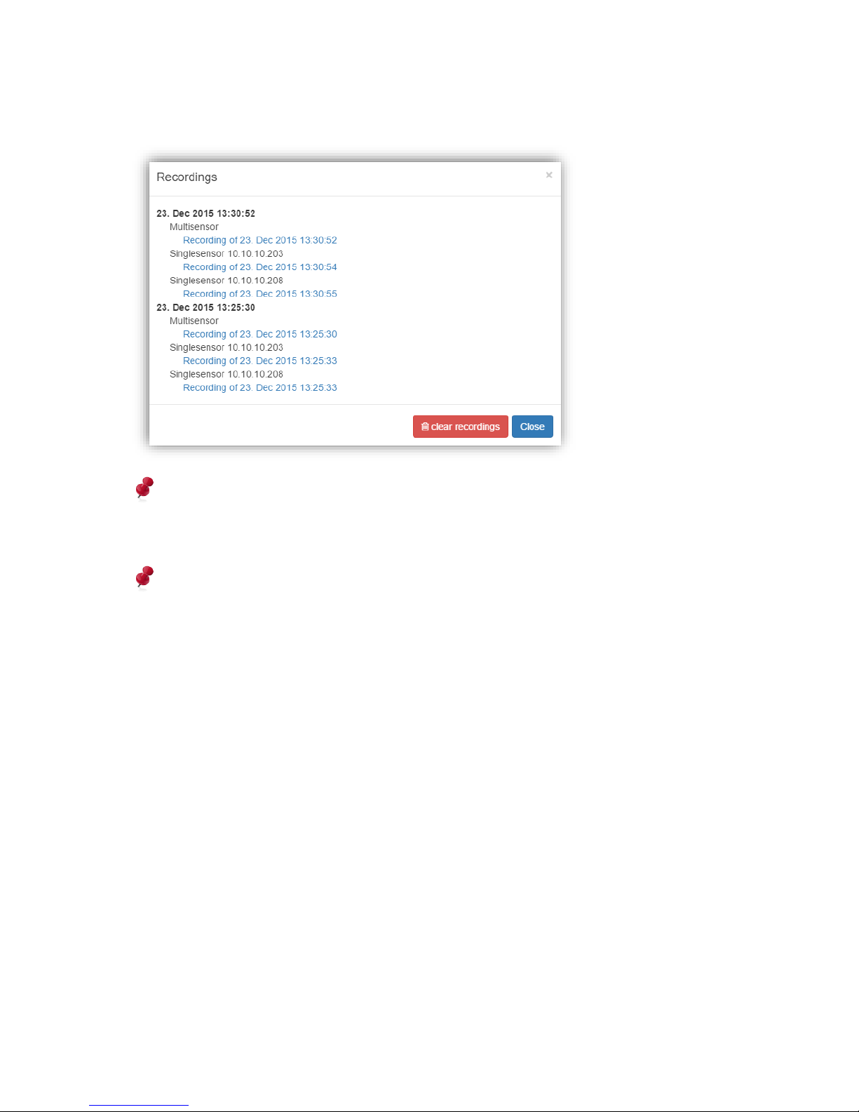
By clicking on “show recordings”, all recorded sequences stored on the sensors are
displayed:
All sequences are grouped into their corresponding recording, displayed with the date of the
latest sequence of every recording. A single sequence file can be downloaded by clicking on
it. To analyze a complete recording, all sequence files should be downloaded in one
directory. The Xovis Validation Viewer can then interpret all these single sequence files as
one recording and display the recording accordingly.
The button “clear recordings” allows to remove all sequence files from the sensor.
3.2.8.4.3. Multisensor Validation Recording
The multisensor supports validation recordings as well. The operation and management of
recordings is equal to the behavior on singlesensor. The only difference is, that, when
scheduling a validation recording, the user gets asked to also schedule validation recordings
on all participating slave sensors:
This is highly recommended for a ground-truth analysis of a multisensor. The Xovis
Validation Viewer supports multisensor validation including belonging singlesensor slave
recordings.
Page 48
48 / 99 www.xovis.com
Belonging singlesensor recordings will also be listed in the “show recordings” modal in the
multisensor view and can directly be downloaded here:
Please note, that when using Validation Recording data push (see chapter 3.2.10.4.2) on
the multisensor master sensor, only the recording files from the master device will be
pushed. All participating singlesensor slaves need to also have data push configured if
common provisioning of these files is desired on the remote side.
Please see the Xovis Validation Viewer manual to learn how to evaluate validation
recordings offline.
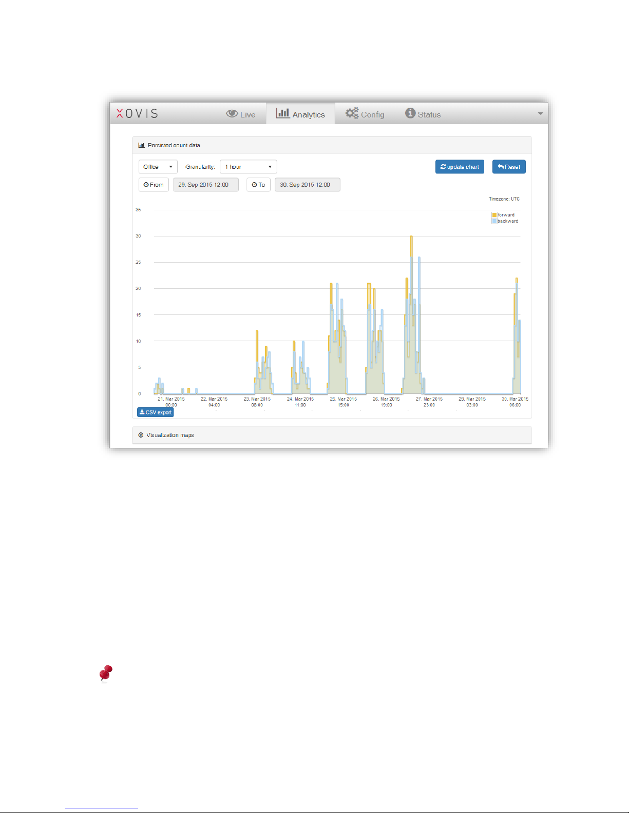
3.2.9 Analytics View
The analytics view contains two boxes named “Persisted count data” and “Visualization
maps”. With the persisted count data box it’s possible to display custom charts of the
persisted count data. The visualization maps box allows to display the start/stop, height and
heat map based on persisted data on the sensor.
Page 49
49 / 99 www.xovis.com
3.2.9.1 Persisted count data
To display the count data based on a specific time frame, start by selecting the count item of
interest in the first drop-down menu. Both, count lines as well as count zones with activated
data persistence are listed.
The second drop-down menu allows the user to choose a granularity. The following
granularities are available: 1 minute, 5 minutes, 15 minutes, 30 minutes, 1 hour, 6 hours, 12
hours, 1 day.
With the “From” and “To” buttons, the time range can be specified on a minute basis.
After selecting the properties, the chart can be updated by clicking on the “update chart”
button.
To reset the properties to the default values and display the chart accordingly, the “reset”
button can be clicked.
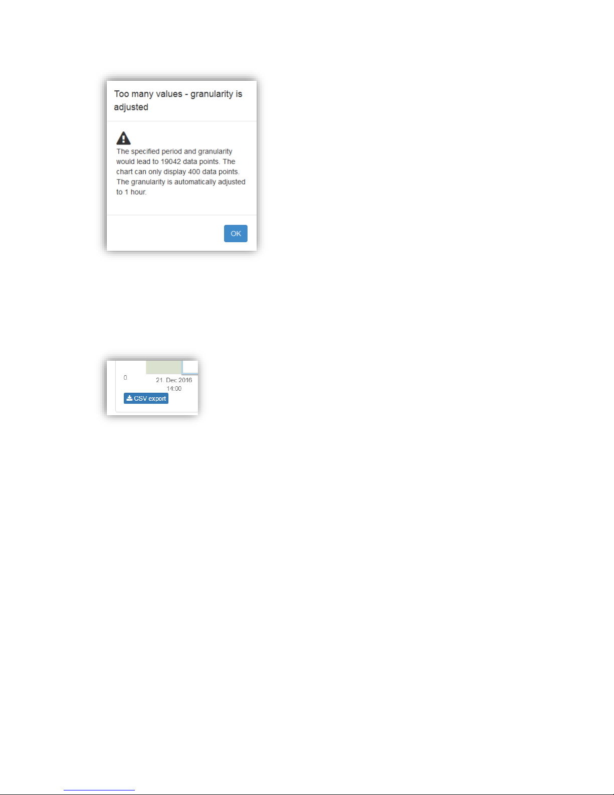
The chart in the statistics view can only display 400 data points in a meaningful manner.
When choosing a granularity and period which would lead to more than 400 data points, a
warning message will be displayed and the granularity will automatically be reduced to the
next coarse value that will lead to 400 values at maximum (see Figure 43).
Page 50
50 / 99 www.xovis.com
Figure 43: Warning of too many data points
Persisted count line data can be exported to a CSV file by clicking on the “CSV export” button
located all on the bottom of the dialog:
All settings are also applied to the CSV export, e.g. the chosen granularity and period.
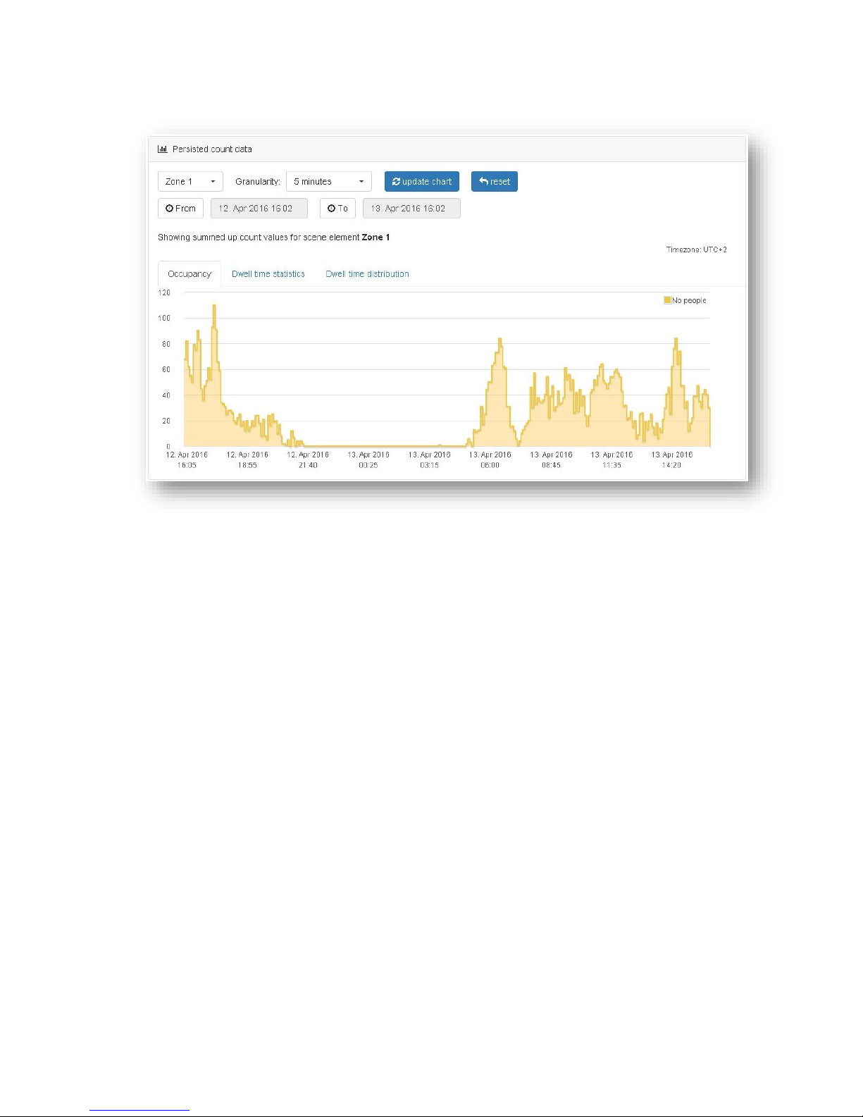
3.2.9.1.1. Count zone charts
When displaying the persisted data of a count zone, a tab navigation offers three types of
charts:
Page 51
51 / 99 www.xovis.com
Occupancy
The occupancy shows the number of persons that have been measured within the zone at the
end of each time-bin. When changing the granularity to rougher granularities than “1
minute”, the new time bins will contain the occupancies of their last included minute bin. For
example, when selecting a “5 minutes” granularity, the bin from 9:00 to 9:05 will contain the
occupancy level of the persisted value from 9:04 to 9:05.
Page 52
52 / 99 www.xovis.com
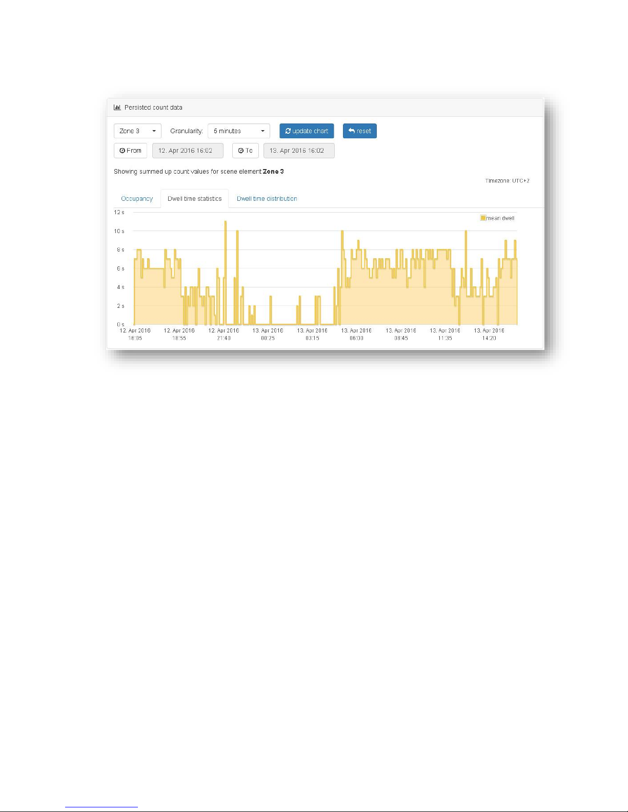
Dwell time statistics
The dwell time statistics value shows the average dwell time during every time bin. When
choosing rougher granularities than “1 minute” the data from the stored 1 minute values are
combined. For correct statistical combination of these dwell times, the sensor internally
stores the number of persons for each 1-minute value and uses a weighted average.
Page 53
53 / 99 www.xovis.com
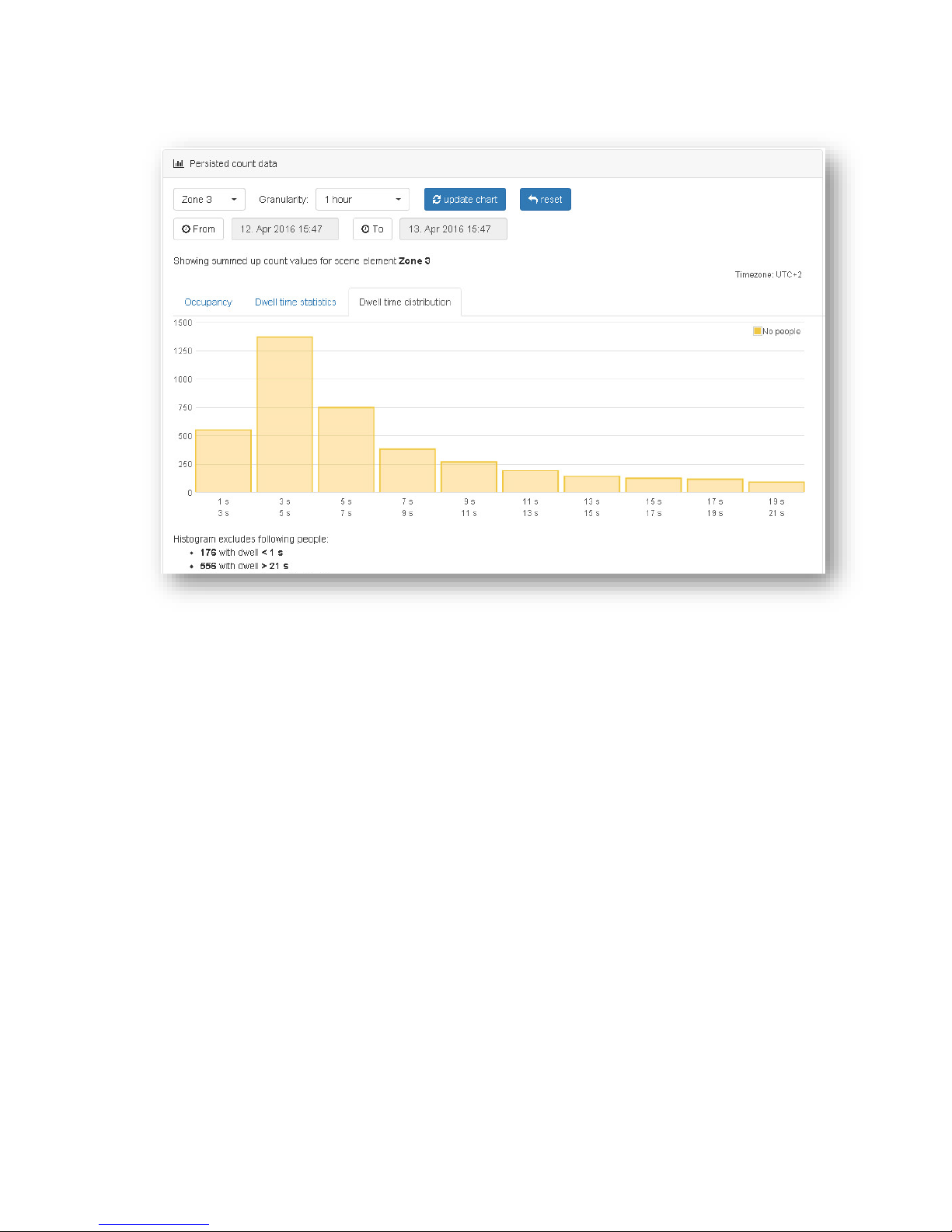
Dwell time distribution
The Dwell time distribution shows a histogram of all dwell times during the selected time
period. The values are shown in 10 equally distributed bins between the minimal dwell time
and the maximal dwell time.
The information text below the histogram shows a list of dwell times which are not
considered in the histogram:
- Too short dwell times: Shows the number of tracks with dwell times, shorter than the
minimal dwell time
- Too long dwell times: Shows the number of tracks with dwell times, longer than the
maximal dwell time
- Invalid tracks: Shows the number of tracks which have not been created and deleted
outside the dwell zone (for further information see the chapter “4.3 dwell zone
placement”)
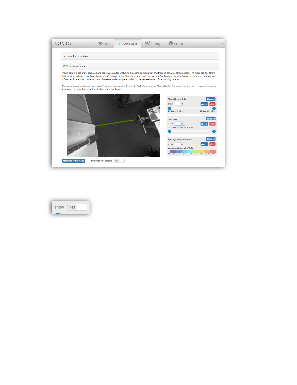
3.2.9.2 Visualization maps
The “Visualization maps” box shows persisted and accurate map data for analyzing the scene
configuration and tracking behavior of the sensor. The maps are built from historic data
gathered directly on the sensor. Compared to the "live maps" from the Live view and Config
view, the visualization maps shown here are not influenced by network connectivity and
therefore hold a complete and accurate representation of the tracking situation.
Page 54
54 / 99 www.xovis.com
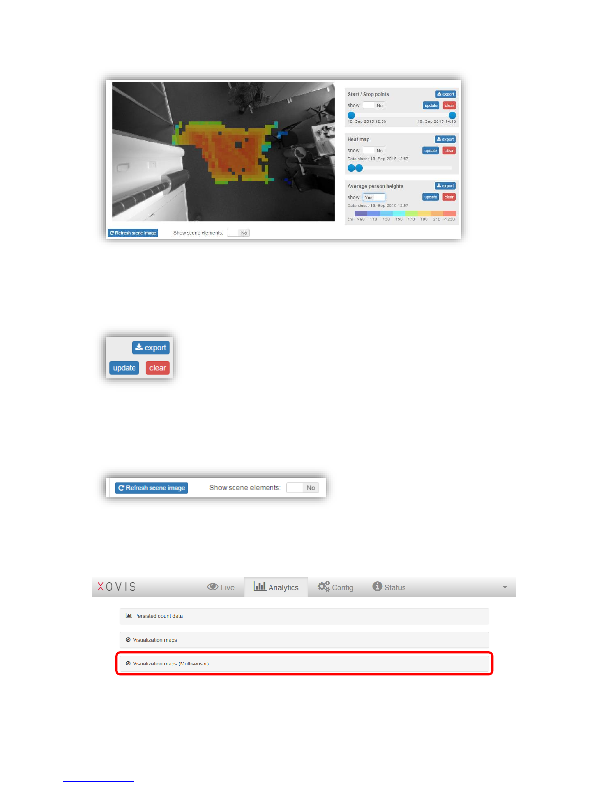
Each single map type can be overlaid on the scene by just toggling the dedicated “show”-
toggle.
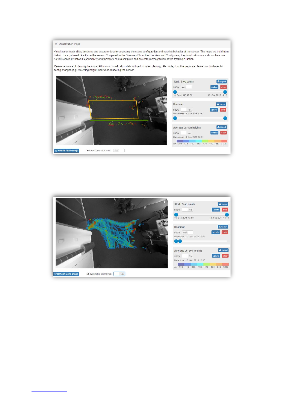
In the next example the Start / Stop points are shown on the scene. The slide bar allows to
navigate through the monitored time period and to visualize the start / stop points depending
on it. Based on this it is now possible to see how the start / stop points have been generated
over the time. The sensor holds the past 10’000 points and will replace the oldest point with a
new one when the limit is reached.
Page 55
55 / 99 www.xovis.com
The heat map shows a dwell-time based coloring of the scene traffic. With the slide bar it is
possible to adjust the saturation. Using it allows to also highlight paths with less traffic.
The Height map displays the average person heights within the scene. This averaged map
can help to if a sensor was moved after configuration. The averaged map will then show a
clear slope. It also helps to validate a proper calibration of the sensor (heights differ too
much from excepted value). The colors are explained in the legend on the side.
Page 56
56 / 99 www.xovis.com
All three maps can be exported to a PNG image. The chosen settings like the time period for
start/stop points or the saturation for the heat map are also applied to the exported images.
All maps can be reset by clicking on “clear”. The user is the asked to confirm the reset. As
these maps are not updated live, for refreshing them the button “update” has to be clicked.
All below the map view, the button “Refresh scene image” allows to re-capture the displayed
scene image. Toggling the switch “Show scene elements” allows to overlay or hide count
lines and count zones. This is very helpful to verify proper drawing of the count items, e.g.
when looking at the start/stop points.
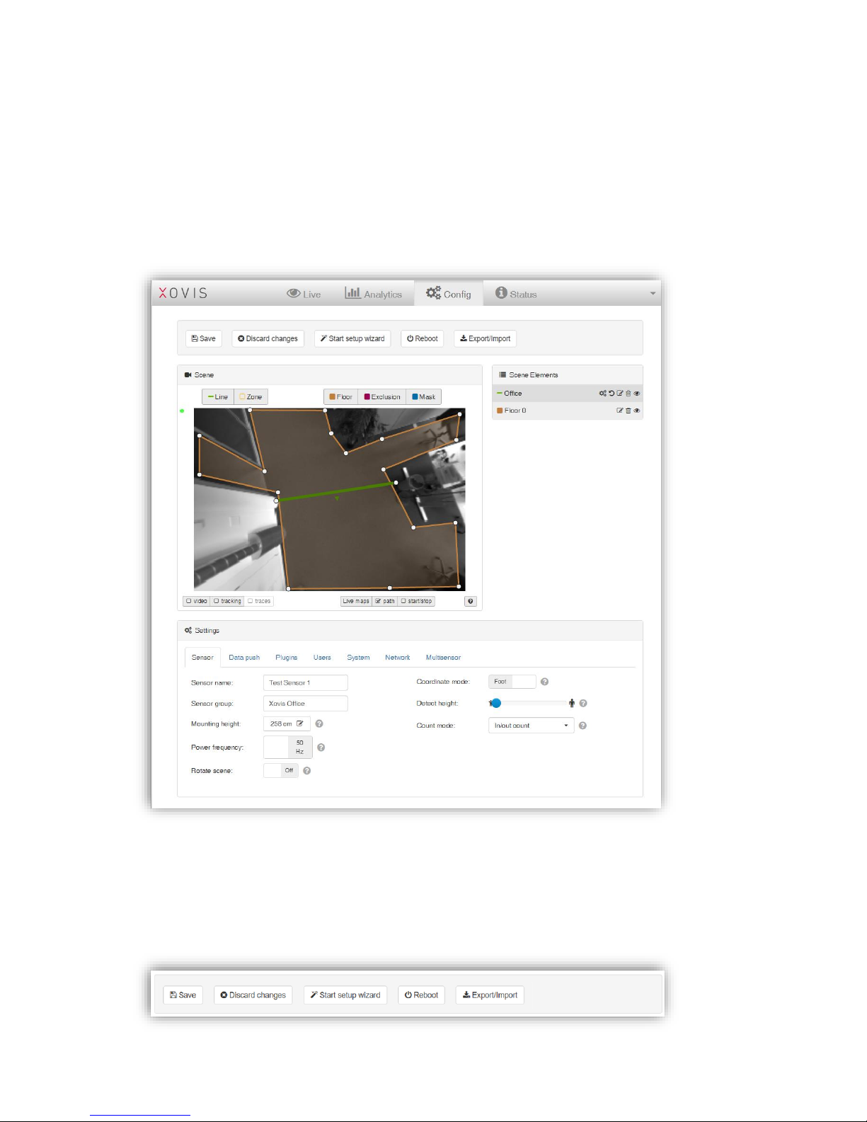
3.2.9.3 Multisensor visualization maps
After configuring a multisensor according chapter “3.2.10.4.7 Multisensor” a third analytics
bar appears:
There are the same features accessible like for a single sensor:
- Start / Stop points
Page 57
57 / 99 www.xovis.com
- Heat map
- Average person heights
Please note that the map controlling elements are located on the bottom of the background
image here, other than with the single sensor “visualization maps”.
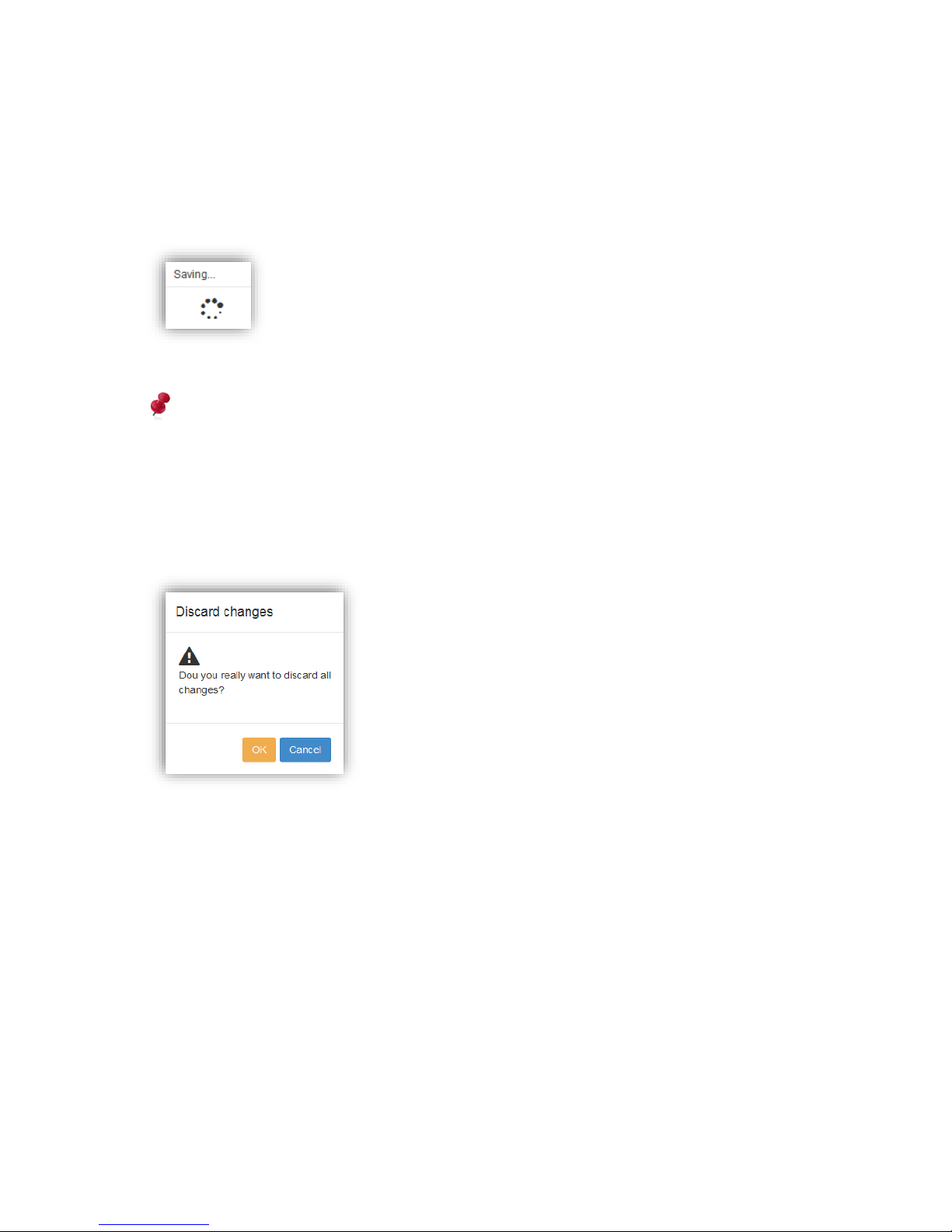
3.2.10 Config View
The config view allows the complete configuration of the sensor. However, it is usually
recommended to configure the sensor using the setup wizard (explained in chapter 3.2.7).
The config view is divided into four parts:
3.2.10.1 Control buttons
Page 58
58 / 99 www.xovis.com
3.2.10.1.1. Save
The “Save” button applies all settings to the sensor. Depending on the changes made, the reinitializing of the sensor after configuration changes can take up to 20 seconds.
While applying the settings and re-initializing the sensor, the web GUI is blocked with the
following indicator:
Figure 44: Configuration save indicator
Important: All changes made in the config view will first be applied to the sensor when
pressing the “Save” button.
3.2.10.1.2. Discard changes
The „Discard changes“ button discards all changes made since saving the last time.
Discarding the changes will prompt for a confirmation:
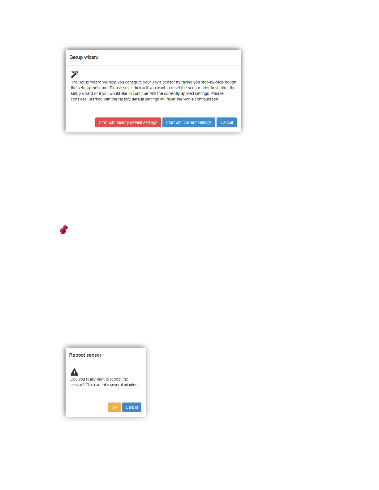
3.2.10.1.3. Start setup wizard
The “start setup wizard” button allows to re-start the setup wizard at any time. When clicking
this button, the user gets asked to choose to either start the wizard with the currently
applied settings or by first resetting the sensor to the factory-default configuration:
Page 59
59 / 99 www.xovis.com
“Start with current settings” is recommended when the user just wants to use the wizard for
updating some parts of the sensor configuration, e.g. the coordinate mode or the count
elements.
“Start with factory default settings” is recommended when the user wants to start the
configuration completely from the beginning with a fresh, un-configured device as it gets
delivered right out of the factory. All settings will then be reset to their origin state expect the
network configuration. This ensures that the sensor will still be reachable under the same IP
address after applying the factory default settings.
Attention: Applying the factory default settings will delete all custom made settings,
including all count elements. All stored count data will be removed irreversibly!
After choosing to start the wizard with or without resetting the settings, the start page of the
wizard will be displayed.
3.2.10.1.4. Reboot
The “Reboot” button allows the user to reboot the sensor. This can be necessary for example
when configuration changes are made on a DHCP based network and the network clients
need to reassign their leases anticipated.
After pressing this button, the user is asked to confirm the requested reboot.
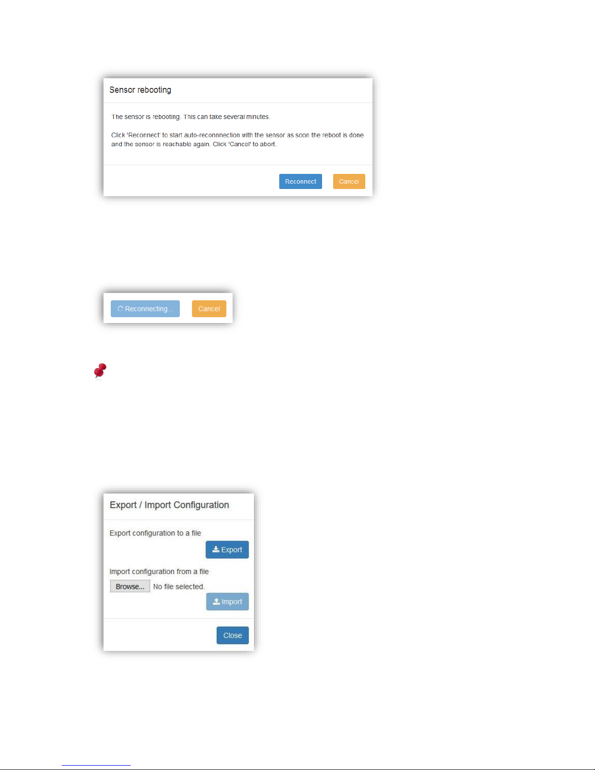
When clicking “OK”, the sensor will reboot which usually takes about 2 minutes. The
following dialog will be displayed:
Page 60
60 / 99 www.xovis.com
By clicking “Reconnect”, the web GUI will automatically poll the sensor to observe when it is
back online and then automatically reconnect the web GUI. While waiting for the sensor to be
online again, the “Reconnect” button will indicate the reconnection with a rotating spinner
icon as shown in Figure 45:
Figure 45: Reconnecting to the web GUI while rebooting
Reconnection will fail if the sensor is assigned to a different IP address by the DHCP
server after rebooting.
3.2.10.1.5. Export/Import
The “Export/Import” button offers a convenient way to save the whole sensor configuration to
a file or to import and apply a configuration from such a file.
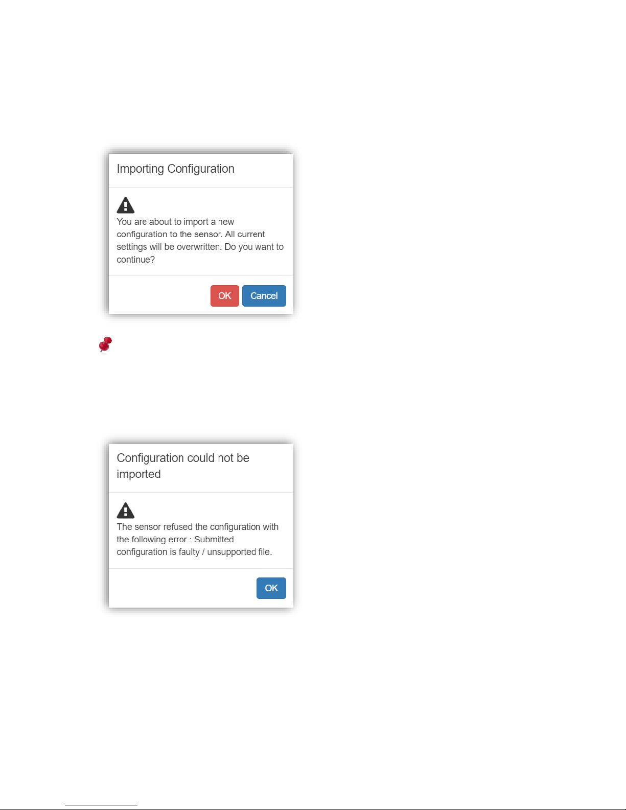
By clicking the button, the following dialog offers these two options to the user:
Clicking on “Export” leads to a download of the sensor configuration file. Depending on the
browser settings, the file is automatically downloaded to a default folder or the user gets
asked where to save the file.
Page 61
61 / 99 www.xovis.com
For importing a sensor configuration from a configuration file stored locally on the user’s
computer, the user simply can browse for the file by clicking on “Browse…”. After selecting
the desired file, the import is started by clicking on “Import”.
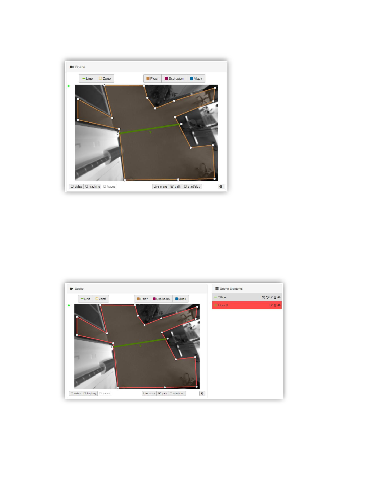
The user then is asked to confirm the import process of the configuration.
Please be aware, that the configuration currently applied to the sensor will be completely
overwritten by the imported configuration.
If the file trying to import is not a valid Xovis PC-sensor configuration file or the configuration
is not applicable to the sensor, the user gets notified by a respective message dialog:
Page 62
62 / 99 www.xovis.com
3.2.10.2 Scene view
Similar to the “Scene live view” in the live view (see chapter 3.2.8.1) the “Scene” box holds
the live view of the sensors scene. All configured scene elements are overlaid in the scene
image. The monitoring can be controlled by the scene view controls described in chapter
3.2.7.9.3.
When hovering over the count elements within the scene, the element gets hightlighted both
within the scene and within the “counts” list (mentioned in the next chapter). When clicking
on a specific element, it gets marked red both within the scene and within the “counts” list.
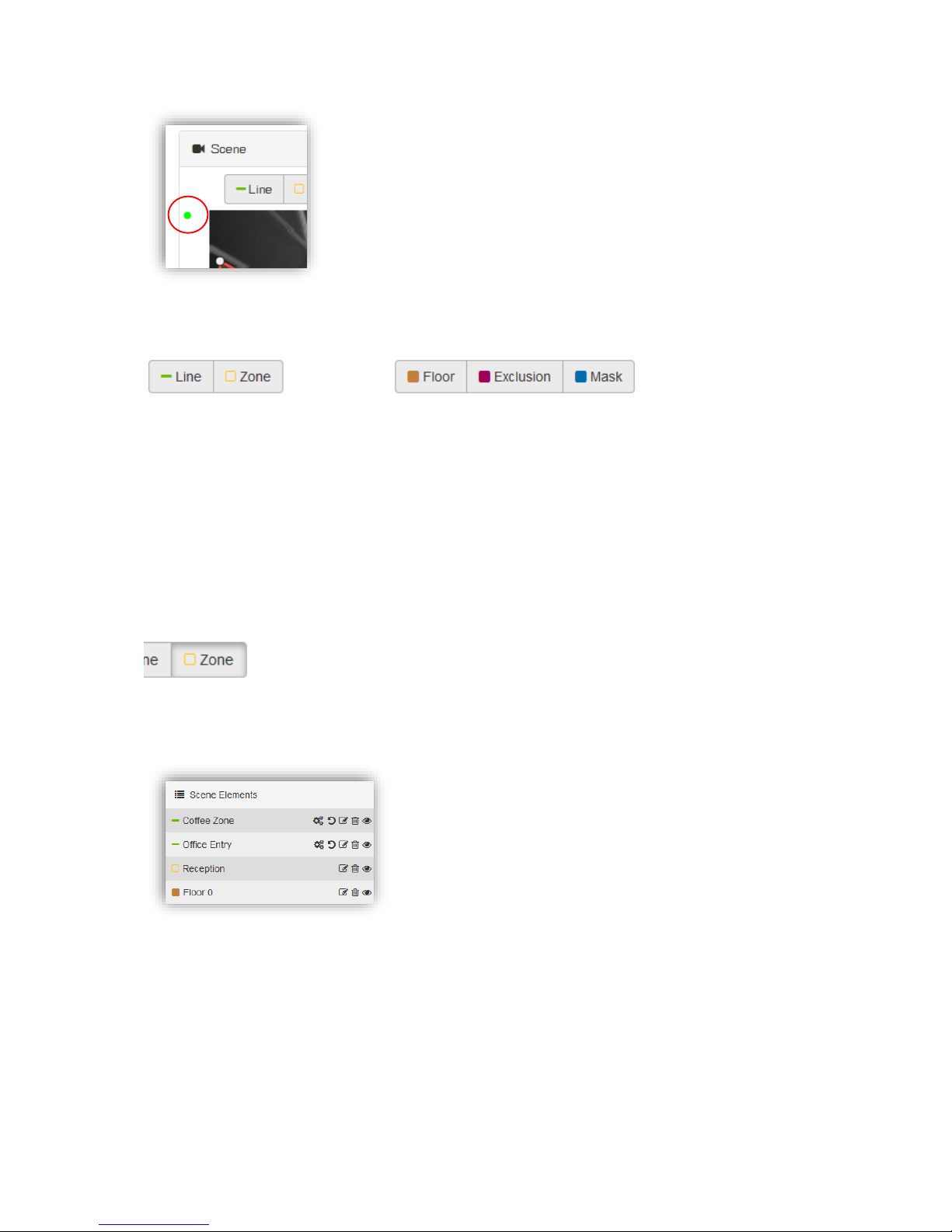
The blinking small green dot displayed in the upper left corner of the “Scene” box indicates
an intact connection to the sensor.
Page 63
63 / 99 www.xovis.com
In addition, the “Scene” box now holds a series of drawing buttons located over the scene
image:
These buttons allow the user to add new scene elements like count lines and zones but also
floor, exclusion and taboo masks.
The drawing procedure and functionality of count lines, count zones and floor masks are
described in chapters 3.2.7.6, 3.2.7.9.4 and 3.2.7.9.5. Please refer to these chapters to learn
about the functionality and purpose of the scene elements. The exclusion and taboo masks
(violet and blue icon) are used rarely and only for troubleshooting. The drawing procedure is
the same as for floor masks. The meaning and usage of exclusion and taboo masks will be
explained in the troubleshooting section in chapter 4.2.
The currently active drawing tool is indicated as a pressed button as shown in Figure 46:
Figure 46: Active drawing tool
3.2.10.3 Scene elements
The “Scene elements” box has already been explained in chapter 3.2.7.9.6. The functionality
and purpose in the config view is exactly the same. Other than during the setup wizard, the
floor masks can now be deleted also. Please refer to the mentioned chapter to learn more
about the “Scene elements” box.
Page 64
64 / 99 www.xovis.com
3.2.10.4 Settings
The “Settings” box holds elements for all settings of the sensor. Most of these settings are
part of the setup wizard and it is strongly recommended to setup a PC-Series sensor by
using the wizard (see chapter 3.2.7). However, users familiar with all the settings can change
them here. Beside those basic settings, the “Settings” box also allows to manage users,
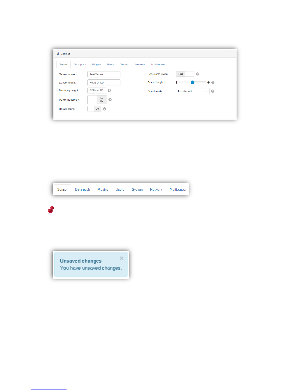
plugins and data push configuration. The settings are divided into 7 sections which can be
displayed using the tab navigation:
Important: All changes made in the config view will first be applied to the sensor when
pressing the “Save” button (see chapter 3.2.10.1.1). An “unsaved changes” reminder
pops-up as soon as any changes will be performed. It will disappear only after clicking on
the save button, by undoing any changes or by clicking the cross symbol on the upper right
side of the blue reminder box.
3.2.10.4.1. Sensor
The “Sensor” section holds all parameters relevant to the counting / tracking functionality of
the sensor as well as the sensor identification fields “Sensor name” and “Sensor group”. All
these settings have already been described in chapter 3.2.7 “Setup Wizard”.
3.2.10.4.2. Data Push
This section allows to manage the data push capability of the sensor. Using data push, the
sensor can automatically inform a remote point about count data, person coordinates,
sensor status or validation recordings. These data can be pushed using HTTP(S) and (S)FTP.
Page 65
65 / 99 www.xovis.com
Please refer to the API documentation to learn more about the data push mechanism
including formats and requirements to the remote destination.
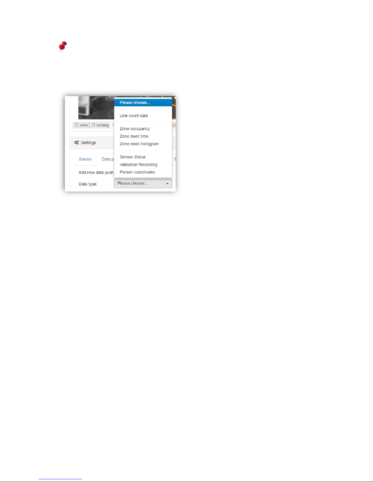
To add a new data push agent, first the data type has to be selected:
As soon the data type is set, all remaining fields will appear and let the user select:
- The interval: How often the data shall be pushed.
- The Granularity (for line & zone data and person coordinates only): Which granularity
to apply to the count data or person coordinates. See chapter 3.2.9.1 “Persisted
count data” to learn more about granularity for count data.
- The protocol: Which method to use for pushing the data (HTTP(S), FTP or SFTP/SSH,
validation recording uses FTP/SFTP only).
- Data push format (for line & zone data only): Which data format to use for the pushed
data (XML v2 or JSON). For legacy reason, line count data offer XML v1 as well.
- All parameters required for the chosen protocol.
For pushing with FTP and SFTP/SSH a custom port can be specified by just declaring it after
the host (IP or domain) separated by a colon (“:”).
When pushing using HTTP(S), only the URL needs to be specified. The URL requires to
declare the protocol which can be http:// or https://. Please refer to the RFC 3986 declaration
to learn more about URL format. Figure 47 shows an example of count data push
configuration using HTTP(S):
Page 66
66 / 99 www.xovis.com
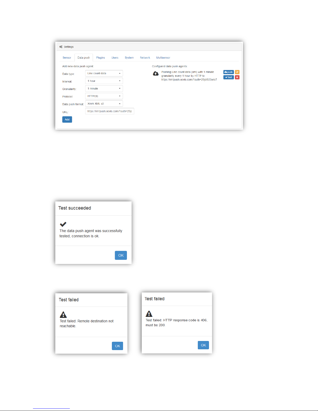
Figure 47: Example configuration for pushing count data to remote destination
This setup will push count data of 1 minute granularity every hour to rmtpush.xovis.com with
a custom URL parameter “auth”.
The “test” button allows to instantaneously test the connectivity to the remote destination.
When clicking on it, the sensor tries to send a sample message to the specified destination.
The status is the shown to the user in the Web GUI:
If testing fails, the error is added to the status message to support the debugging procedure:
Page 67
67 / 99 www.xovis.com
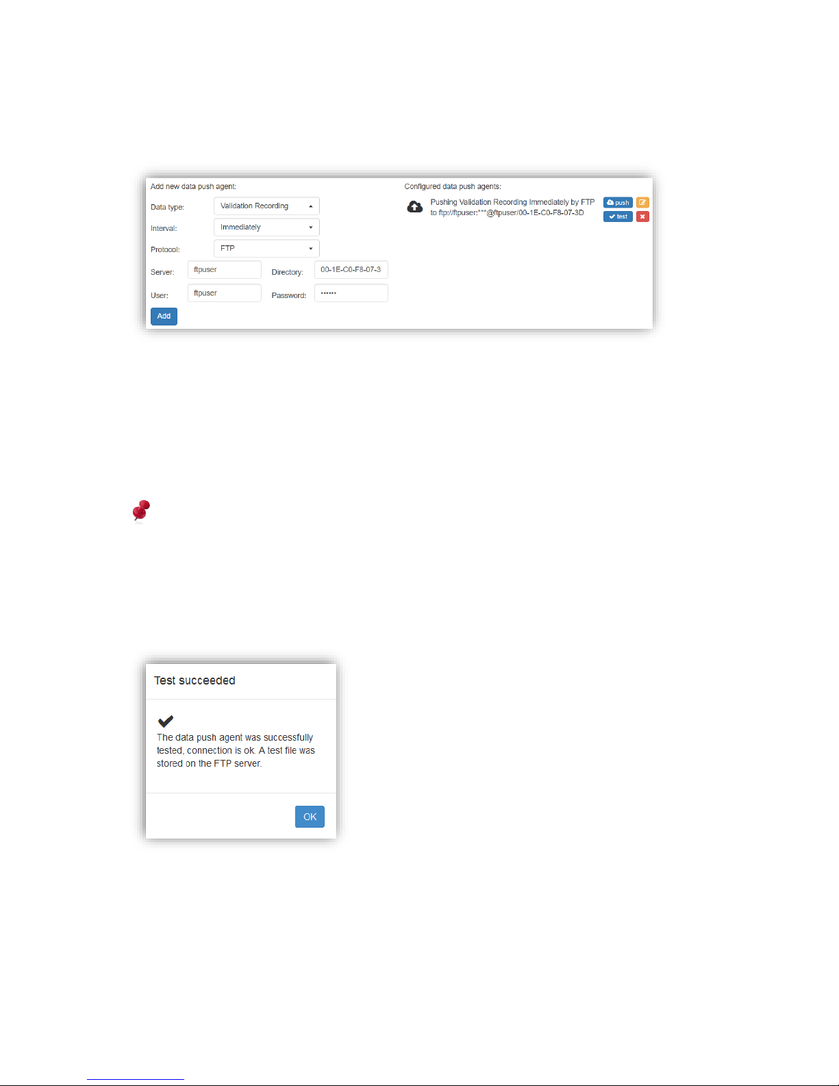
When pushing using FTP or SFTP/SSH, the server and login credentials need to be provided.
Optionally a directory can be specified. The following figure shows an example of validation
recording push configuration (only FTP/SFTP is supported for validation recording):
Figure 48: Example configuration for pushing validation recordings to remote destination
This setup will push validation recording sequences immediately, i.e. directly after a
sequence file is stored, to the FTP server with IP 10.10.10.88 using user “ftpuser” with a
specified password. The recordings will be stored in the directory /sensor/00-1E-C0-DF-65D9/rec.
The password will never be displayed and will also be stored in an encrypted format on the
sensor. Once set, a password therefore cannot be looked up in plaintext anymore.
As with the count data push agent, connectivity can also be tested using the “test” button. If
the connection succeeds, a file with sample content will be stored on the FTP server. The
status message informs about this:
The sensor supports up to 8 data push agents. A configured data push agent can be removed
by clicking on the “remove” button on the right side of every agent.
As with the whole config section, changes to the data push configuration are first applied
when pressing the “Save” button.
Page 68
68 / 99 www.xovis.com
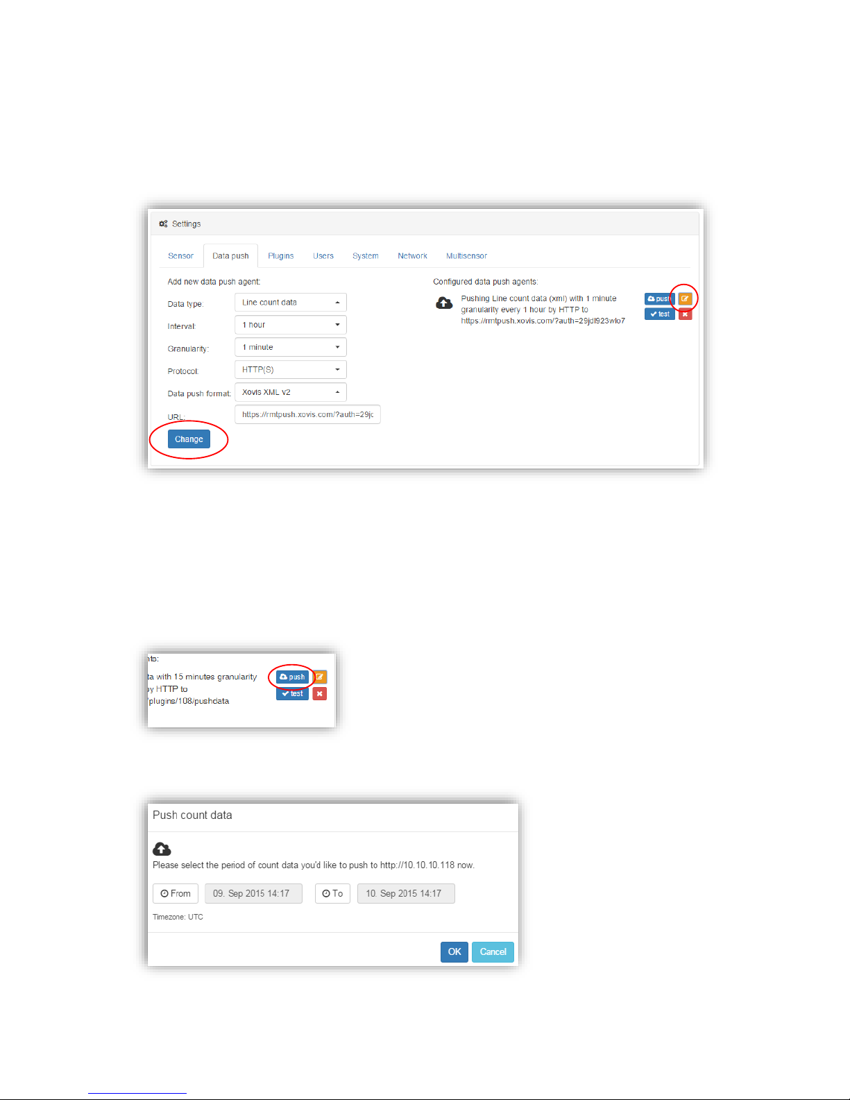
Any already configured push agent can be modified by just clicking on the orange icon
highlighted on the next picture. To confirm any setting changes just click on the button
“Change” and afterwards “Save” again.
The button “push” allows to immediately push count data, sensor status or a validation
recording sequence to the selected destination at any time.
This can be useful for example when a sensor was installed two weeks ago but outgoing
network connectivity was first possible after these two weeks. Using the “manual data push”
functionality now, the count data of these past two weeks can now be pushed to the remote
side manually.
Manually pushing count data allows the user to specify the desired period to push:
Page 69
69 / 99 www.xovis.com
Manually pushing validation recording will transfer all currently stored recordings to the
remote destination and manually pushing the sensor status will push the current sensor
status.
Person coordinates
Person coordinates represent all person positions tracked by the sensor in a defined period
whereby this period is set by the granularity of the push agent. With other words, the
granularity defines the resolution of person tracks. As finer the granularity, as higher the
temporal resolution of the pushed coordinates.
Person coordinate push can be compared to the Object Stream functionality (refer to the
respective documentation to learn more about the Object Stream) with the difference, that
the client asking for person tracks does not have to initiate a session and therefore does not
need direct access to the sensor. Using person coordinate push, the sensor can be set to
send person tracks to a remote site even if the sensor is located behind a firewall.
The finest/highest granularity available here is 0.25 seconds, the lowest one is 2.5 seconds.
The interval defines how often the person coordinates shall be transmitted to the remote
site.
Due to the possibly high amount of data, person coordinates are not persisted on the sensor
but only cached. Not all combinations of interval vs. granularity are supported. For example,
when using the largest interval of 1 hour, the finest granularity supported is 2.5 seconds. On
the other hand, when demanding for the finest possible granularity of 0.25 seconds, the
maximum interval period is 30 seconds. The following table shows which granularities are
available at which interval:
Interval
Granularity
5 s
30 s
1 min
5 min
15 min
1 h
0.25 s X X
0.5 s X X
1 s X X X X
2.5 s X X X X X X
Person coordinates do not support manual push as these data are not persisted on the
sensor.
Please refer to the API documentation to learn how to receive and parse person push data.
Page 70
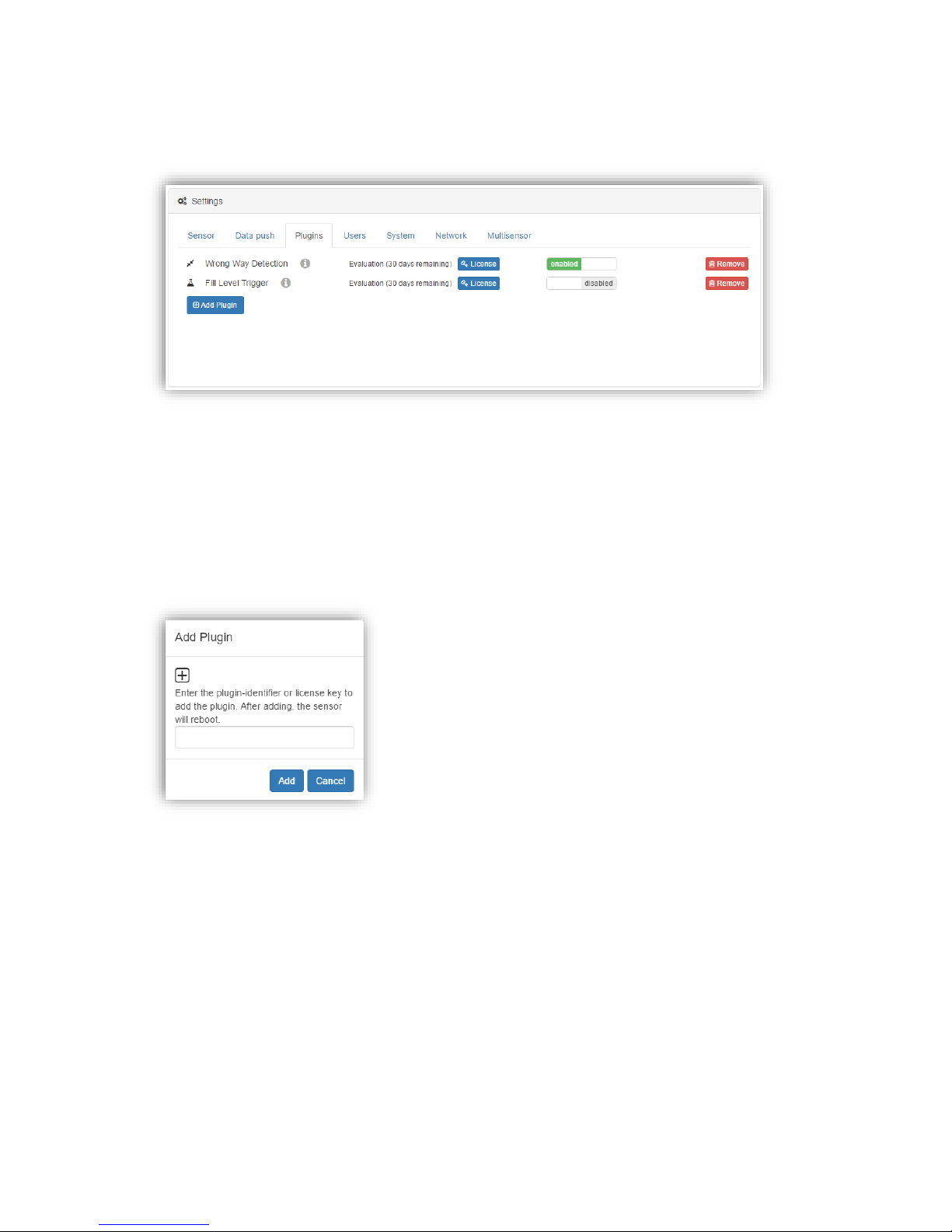
70 / 99 www.xovis.com
3.2.10.4.3. Plugins
The “Plugins” sections shows an overview of all plugins currently activated on the sensor:
By default, the sensor comes with four plugins pre-activated, the “Object Stream” and the
“Event Stream” both, for single-sensor and multi-sensor. These four plugins cannot be
removed. The “Event Stream” plugin is included and free to use, the other plugins can be
evaluated for 30 days (only counting when enabled) and needs to be licensed afterwards.
Please refer to the separate plugin manuals to learn more about these default plugins.
Additional plugins can be added by clicking on the “Add Plugin” button. In the subsequently
dialog, the plugin identifier can be entered. After adding the plugin, the sensor will reboot.
Please contact Xovis to learn more about all available plugins and the respective plugin
identifier, if you are interested in evaluation.
Plugins can be disabled and enabled again by toggling the “enable/disable” switch
accordingly. To license a plugin, the blue “License” button needs to be pressed. In the
following dialog, the license key needs to be entered:
Page 71
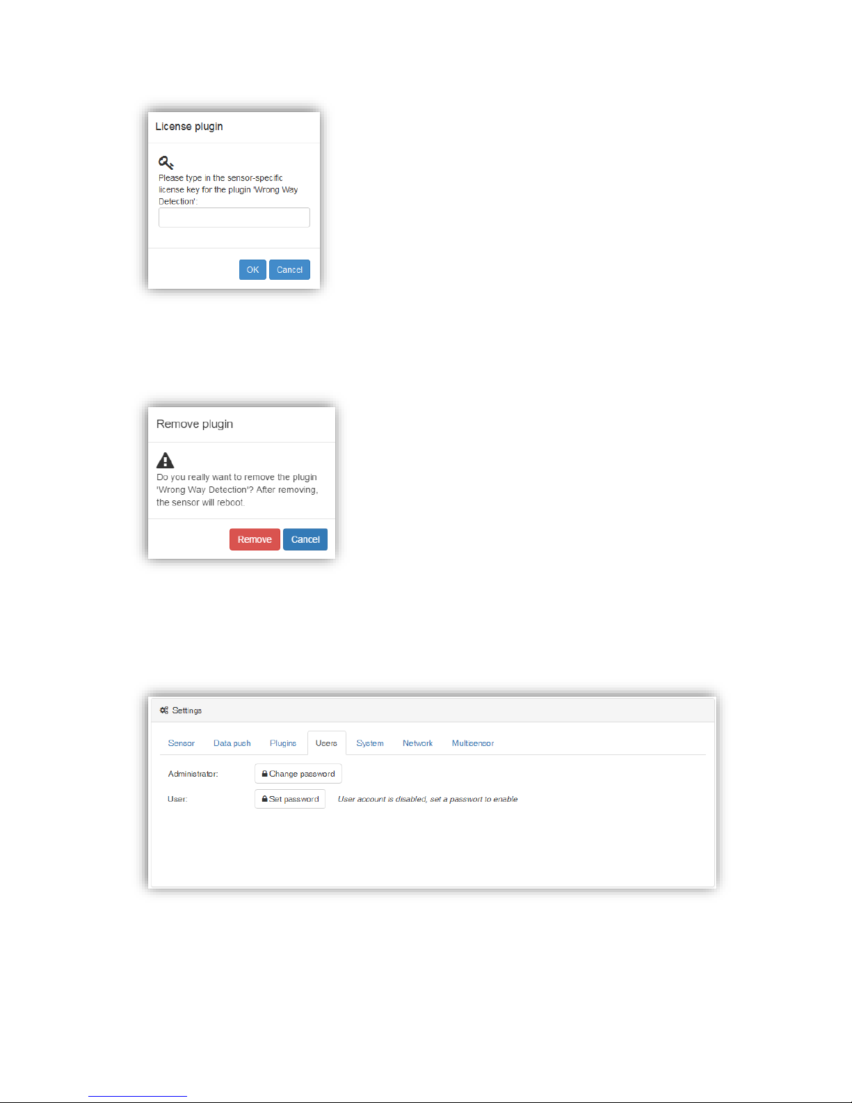
71 / 99 www.xovis.com
Any non-default plugin can also be removed from the sensor. To do so, the red “Remove”
button needs to be pressed. Before the plugin is removed, the user has to confirm a warning
dialog:
After confirming, the plugin will be removed and the sensor will reboot.
3.2.10.4.4. Users
The “Users” section allows to manage the users:
The PC2 sensor offers an Administrator and a User account. The User account is disabled by
default and can be enabled by specifying a password for this user. When the user account is
enabled, the decision to login with one of the two accounts is only based on the password
entered in the login screen. For the case that both accounts, the Administrator and the User,
use the same password, the Administrator user will be logged in.
Page 72
72 / 99 www.xovis.com
The User account offers read-only privileges. When logged in with the User account, the
complete “Config” view is disabled and no operation which could influence the sensors state
can be performed. Figure 49 shows the navigation when logged in with the User account:
Figure 49: Disabled Config view when logged in with User account
When logged in as Administrator and the User account is enabled, the “Users” section
presents a “Disable account” button to disable the User account again (see Figure 50).
Clicking on it will instantaneously disable the user Account.
Figure 50: User account enabled
Page 73
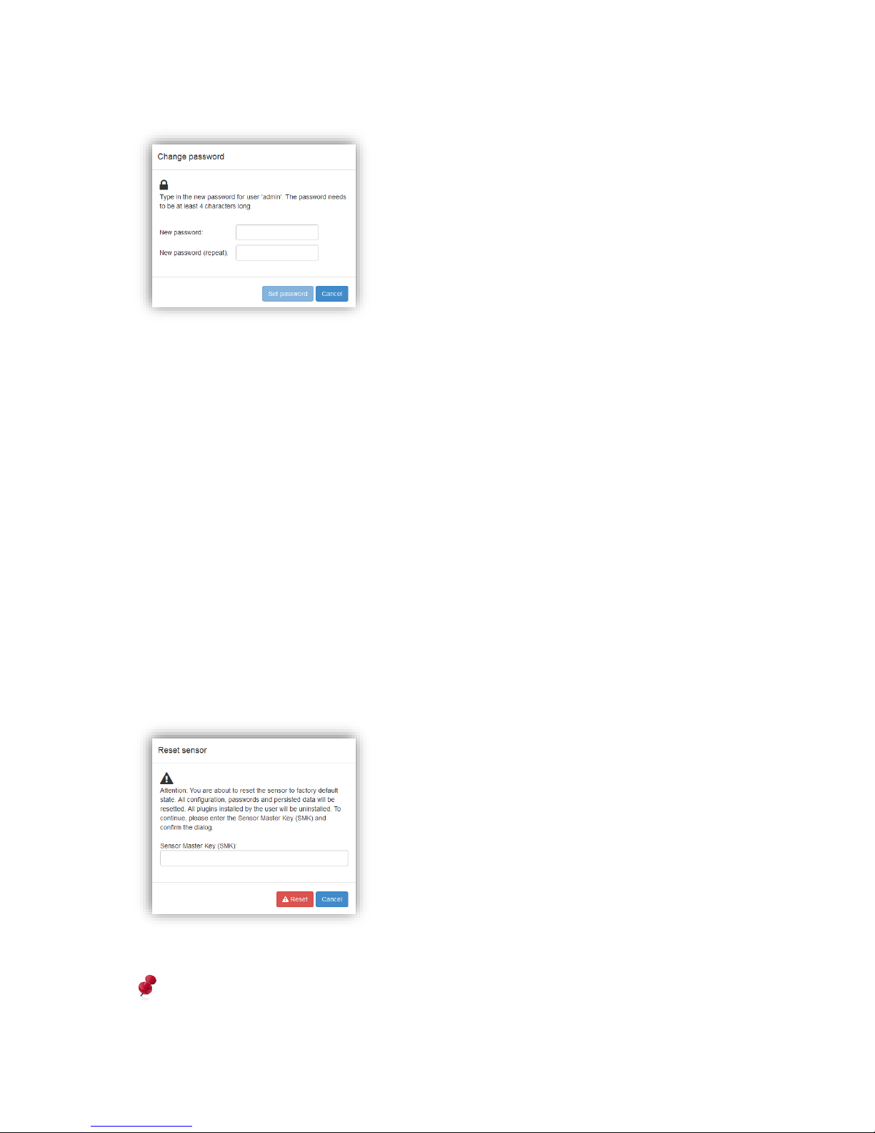
73 / 99 www.xovis.com
Whenever changing or setting a password, the following dialog appears:
To change the password, the user is asked to enter twice the new password for the chosen
user which has to be at least 4 characters long. The new password is set by clicking on “Set
password”. After applying the new password to the sensor, the web GUI will automatically
logout and return to the login screen (see chapter 3.2.5).
3.2.10.4.5. System
The “System” section allows to manage the time zone and the time server or to apply a time
manually, to setup the user interface language, to define the privacy mode level and to
perform a complete sensor reset.
For time zone, sensor time, UI language and privacy mode, please refer to the corresponding
chapters in the wizard section, see chapter 3.2.7 “Setup Wizard”.
The sensor reset allows to complete reset the sensor to its factory state. Other than with the
factory default settings which can be applied when starting the setup wizard (see chapter
3.2.10.1.3), this reset will not only apply the default configuration but will also reset all
passwords, reset all plugins and remove any custom added plugins, remove any validation
recordings, reset the privacy mode to level 0 and enable HTTP again if it was disabled by
configuration. The sensor reset requires the Sensor Master Key (SMK) to be entered:
Please refer to chapter 3.2.7.10 to learn more about the Sensor Master Key (SMK).
Attention: Resetting the sensor will erase any configuration and data and set back the
sensor to the factory default state.
Page 74
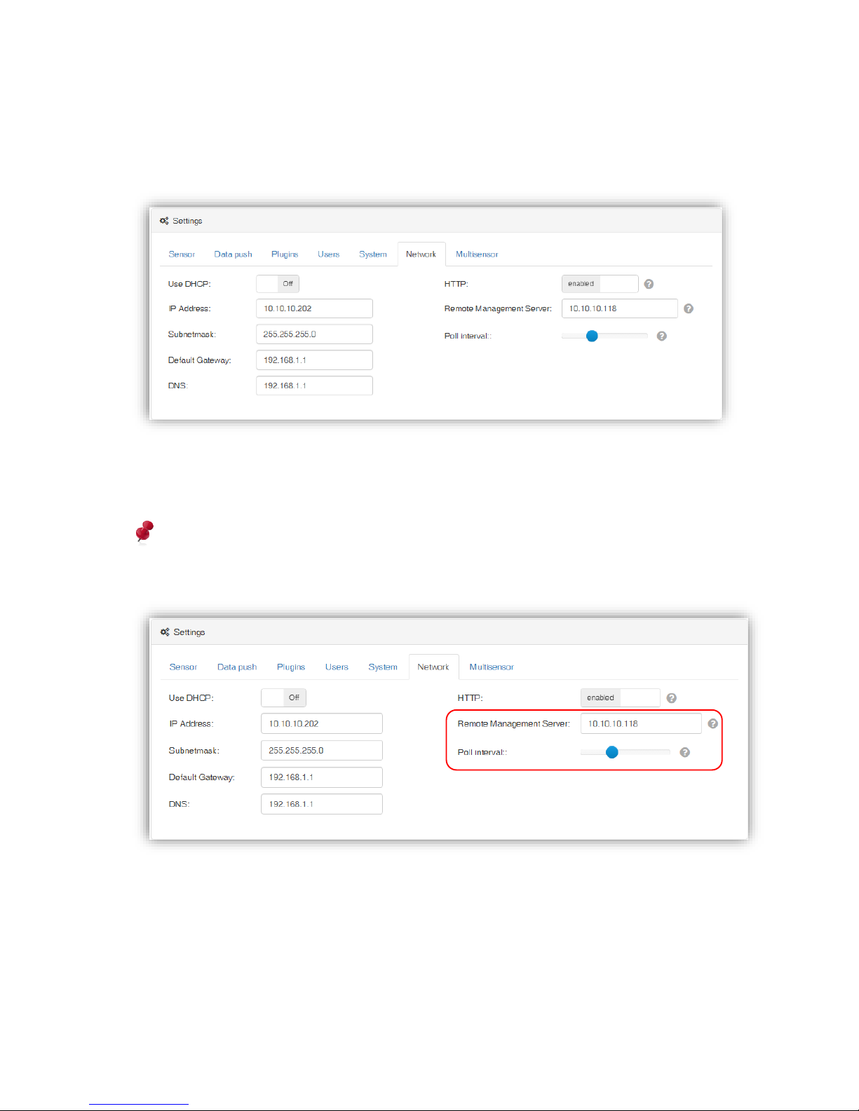
74 / 99 www.xovis.com
3.2.10.4.6. Network
The “Network” section holds the network parameters similar to the corresponding step in
the setup wizard (see chapter 3.2.7.2). In addition it contains the HTTP and Remote
Management Server settings.
The HTTP can be disabled permanently here. This way, any non-encrypted access to the
sensor API and WebGUI is prevented. When toggling this switch to disabled, a popup will
inform the user about the deactivation of the http-WebGUI.
Attention: When disabling HTTP here, the WebGUI will not be reachable anymore under
http://... after saving the configuration.
To allow the communication with the Remote Management Server just enter its URL/IP and
the polling interval. For any further details about the Remote Management Server please
refer to the dedicated documentation.
Page 75
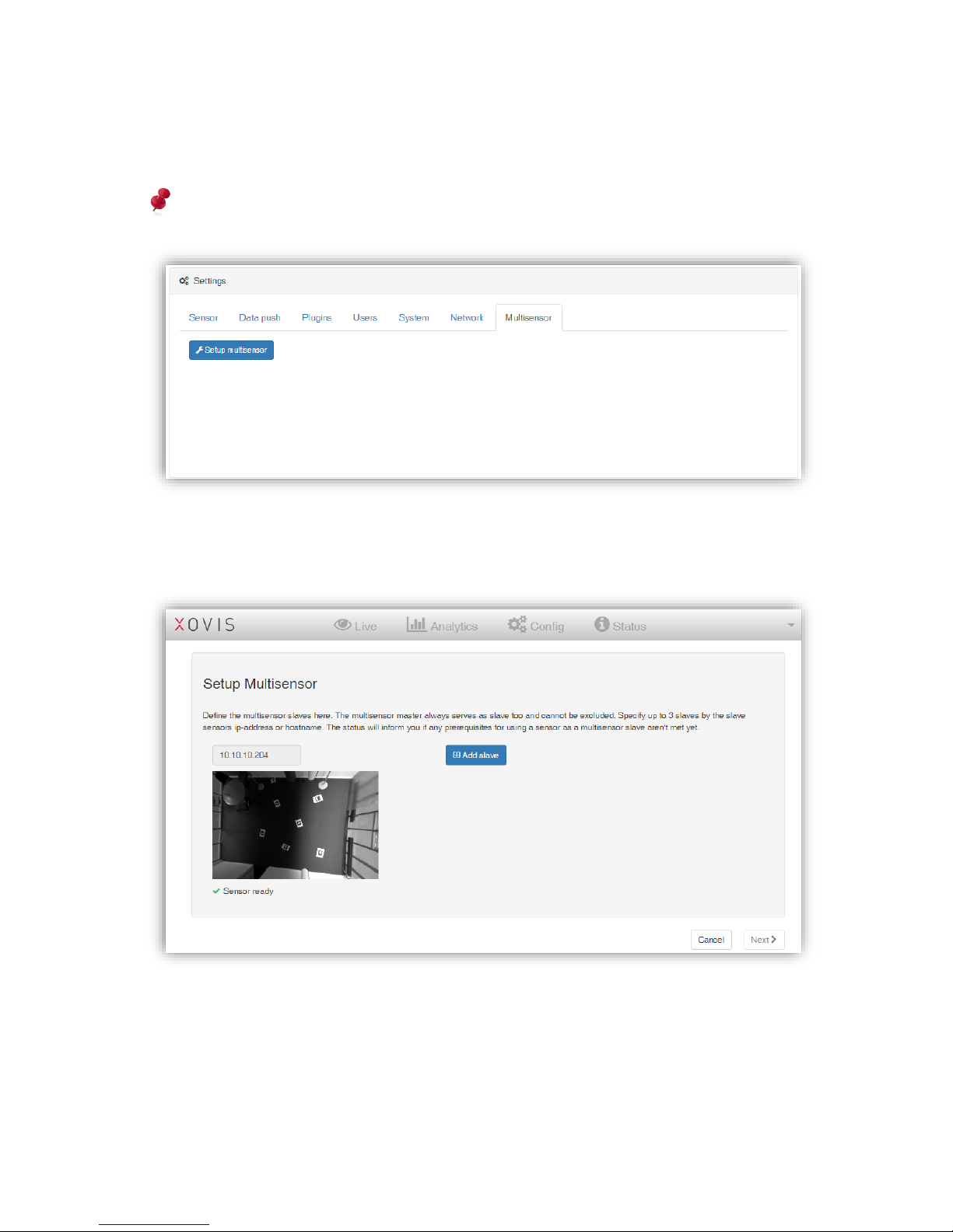
75 / 99 www.xovis.com
3.2.10.4.7. Multisensor
This section allows to configure the multisensor feature. A multisensor today can consist of
up to 9 sensors.
Attention: Make sure that before starting the multisensor configuration each involved
sensor is already configured as single sensor.
With a click on the “Setup multisensor” button the dedicated configuration wizard will start.
In the first screen all involved single sensors can now be added to the multisensor. The
device the multisensor master is running on will always be included here.
Add a sensor by clicking “Add slave” and specify its IP. When leaving the IP field, the wizard
will try to connect to the slave sensor and check, if the slave is ready to become part of a
multisensor.
Page 76
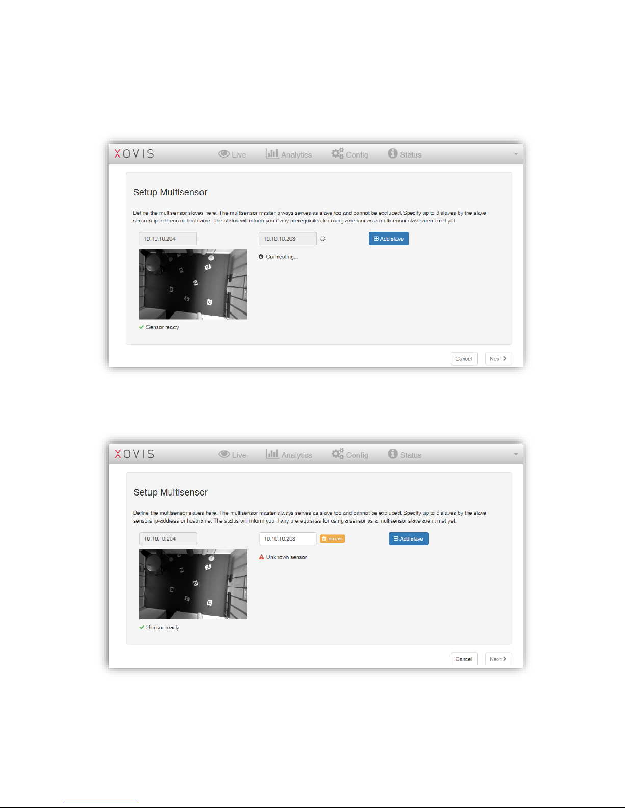
76 / 99 www.xovis.com
This is given when:
- The admin passwords are matching
- The time server is set up
- Privacy Mode is set to 0 or 1
If one of those conditions is not met, an error message will inform the user about the reason.
In this example the IP was wrong and after retrying the sensor availability was confirmed.
Page 77
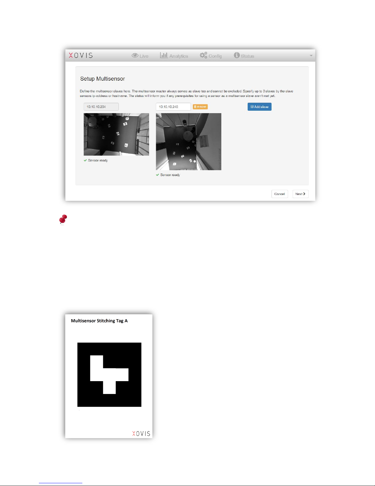
77 / 99 www.xovis.com
Note: The use of different PC-Series models like for example a PC2 with a PC2-UL or a
PC3 is supported. In the above example there is a PC2 on the left and a PC2-UL on the
center.
When all slaves are added, clicking “Next” will bring up the stitching page. The automated
stitching is based on tags which have to be placed underneath the involved sensors with a
distance between each other of minimum 1 meter. Xovis provides a PDF-file
(Xovis_multisensor_stitching_tags_v2.pdf) containing a set of 30 predefined tags, each one to
be printed on an A3-sized paper sheet.
Page 78
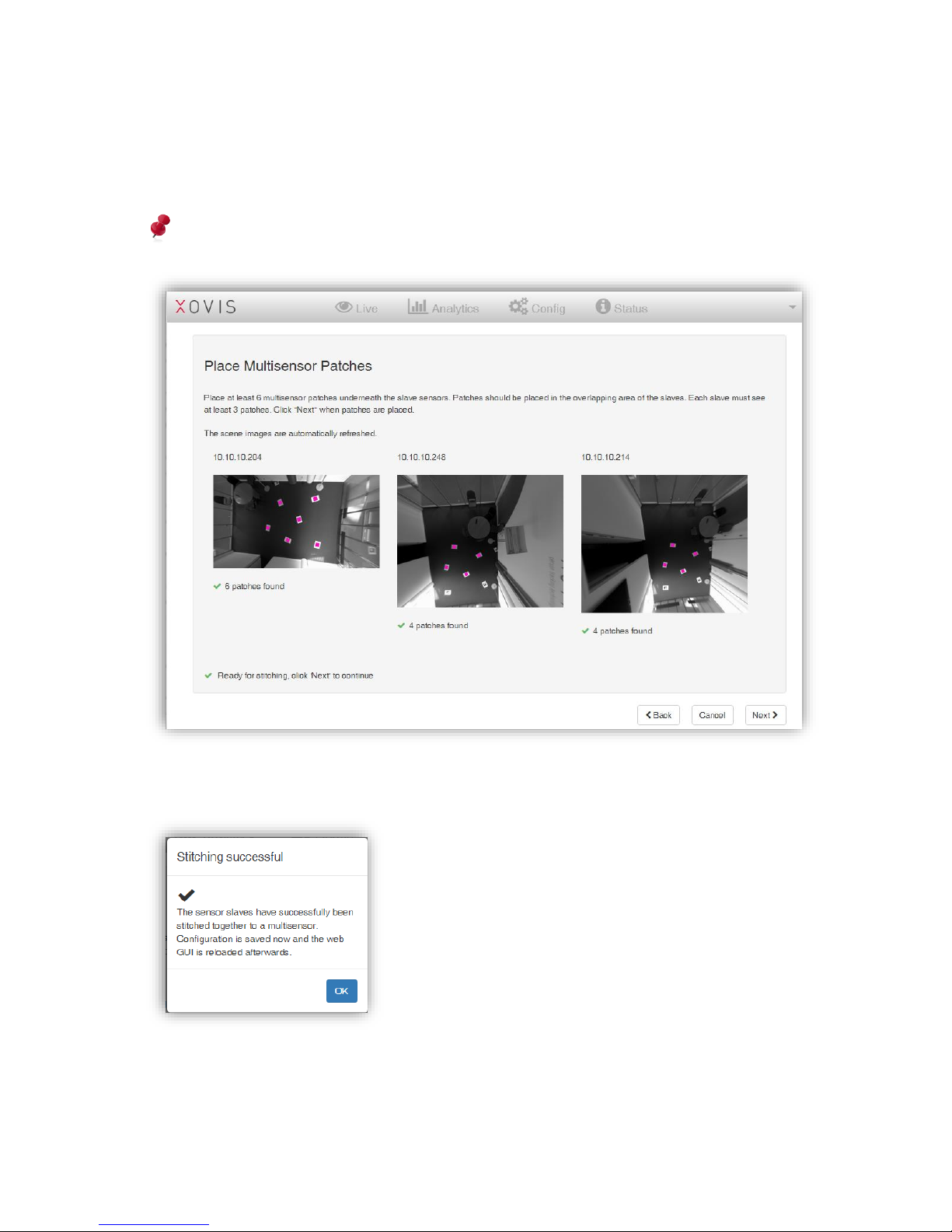
78 / 99 www.xovis.com
On the stitching screen the wizard indicates the number of tags recognized through each
sensor. The accepted tags will be highlighted in purple color. If there are enough visible tags
(at least 3 per sensor), the notification “Ready for stitching” appears on the bottom left side.
Attention: Make sure to never use a specific tag (e.g. ‘A’) more than once in a multisensor
stitching process.
After clicking on the button “Next” the master sensor performs the stitching and confirms it
with the following popup:
After clicking “OK”, the GUI is reloaded. The “Live” and the “Config” tab now contain a “Multi-
Sensor” and a “Single-Sensor”-View.
Page 79
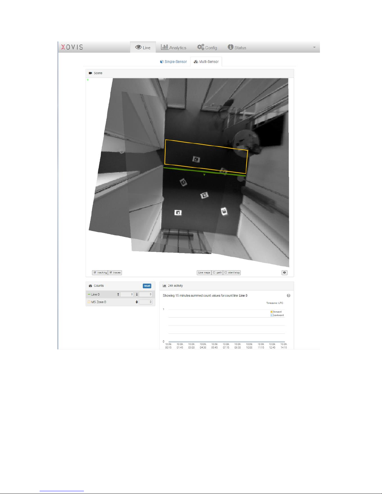
79 / 99 www.xovis.com
The multisensor page on the “Live”-view contains the same four sections as known from the
singlesensor page:
Scene
The “Scene” view shows the stitched still image of the multisensor. It is possible to activate
the tracking (shows the bubbles), the traces and the live maps “path” and “start/stop”.
Counts
The section “Counts” will show the counts of the count lines and zones of the multisensor.
24h activity
The section “24h activity” will show the activities of the last 24 hours with 15 minute
granularity.
Page 80
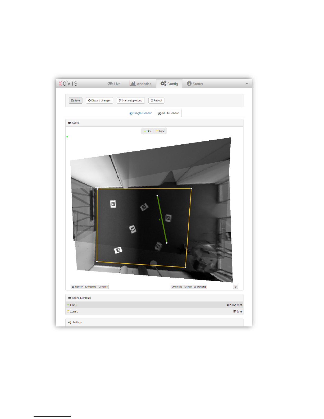
80 / 99 www.xovis.com
Validation Recording
Schedule and manage multisensor validation recordings.
The multisensor view in the “Config” tab allows to setup count lines and zones for the
multisensor:
Likewise when configuring a Single-Sensor, a multisensor allows to draw up to 8 count lines
and zones by using the same drawing method. The drawn multisensor element will be shown
in the section “Scene Elements”.
Page 81
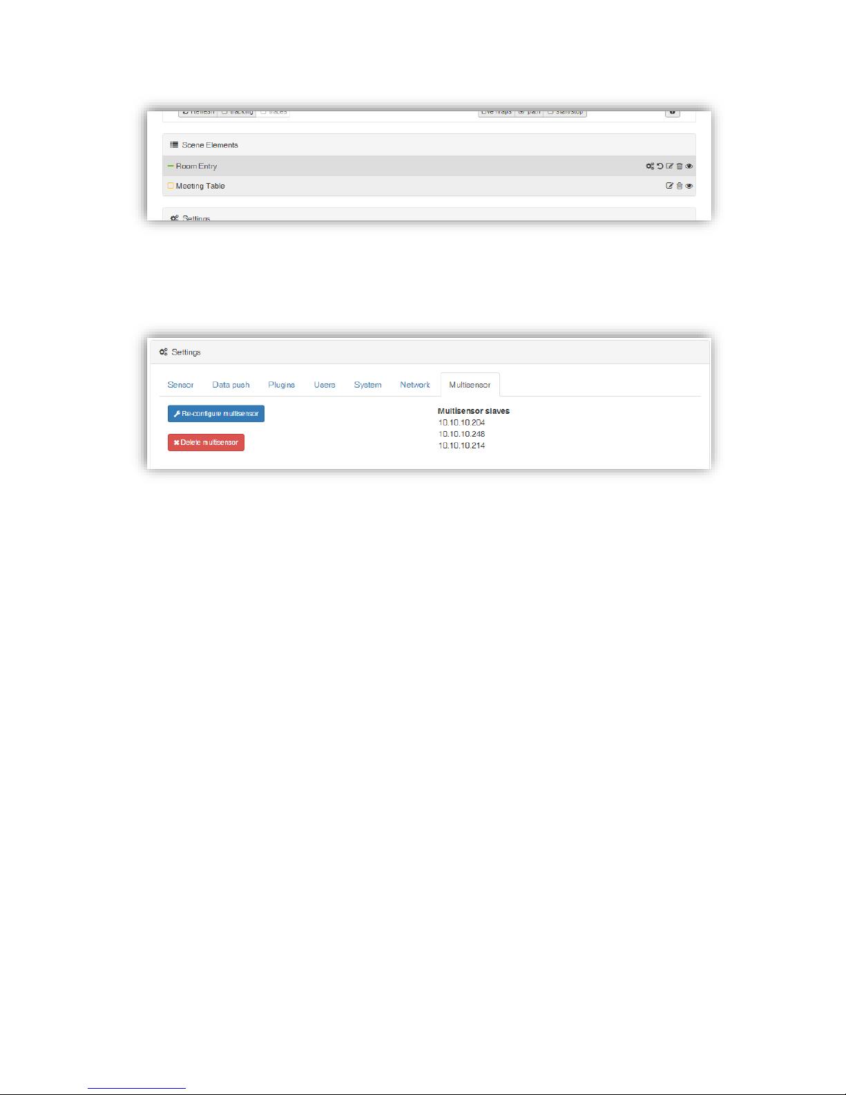
81 / 99 www.xovis.com
The sections “Settings” “Multisensor” contains a list of all involved sensors with their IP
address. Furthermore, the multisensor stitching wizard can be restarted here and the
multisensor can be deleted permanently.
Page 82
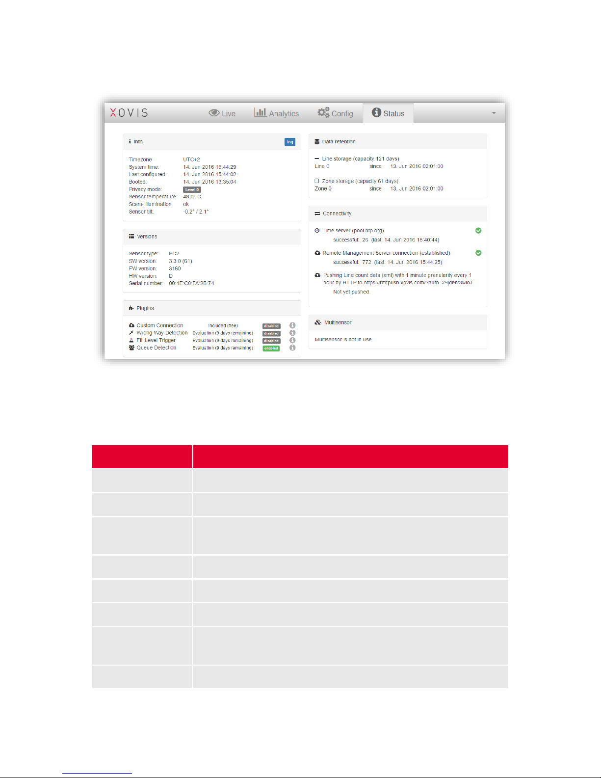
82 / 99 www.xovis.com
3.2.11 Status View
The status view provides various information about the sensor:
3.2.11.1 Info
The “Info” box holds a series of status information of the sensor:
Item
Description
Timezone
The configured time zone, displayed as actual offset from UTC
System time
The sensors internal time/date
Last configured
The time of last configuration change, or “not configured (factory
default)” when the sensor was not yet configured
Booted
The last boot time
Privacy mode
The configured level of privacy (Level 0 – Level 3)
Sensor temperature
The sensors temperature in degrees Celsius
Scene illumination
The illumination status of the scene in which the sensor is
operating, can be “ok” or “insufficient”
Sensor tilt
The current tilt of the sensor
Page 83
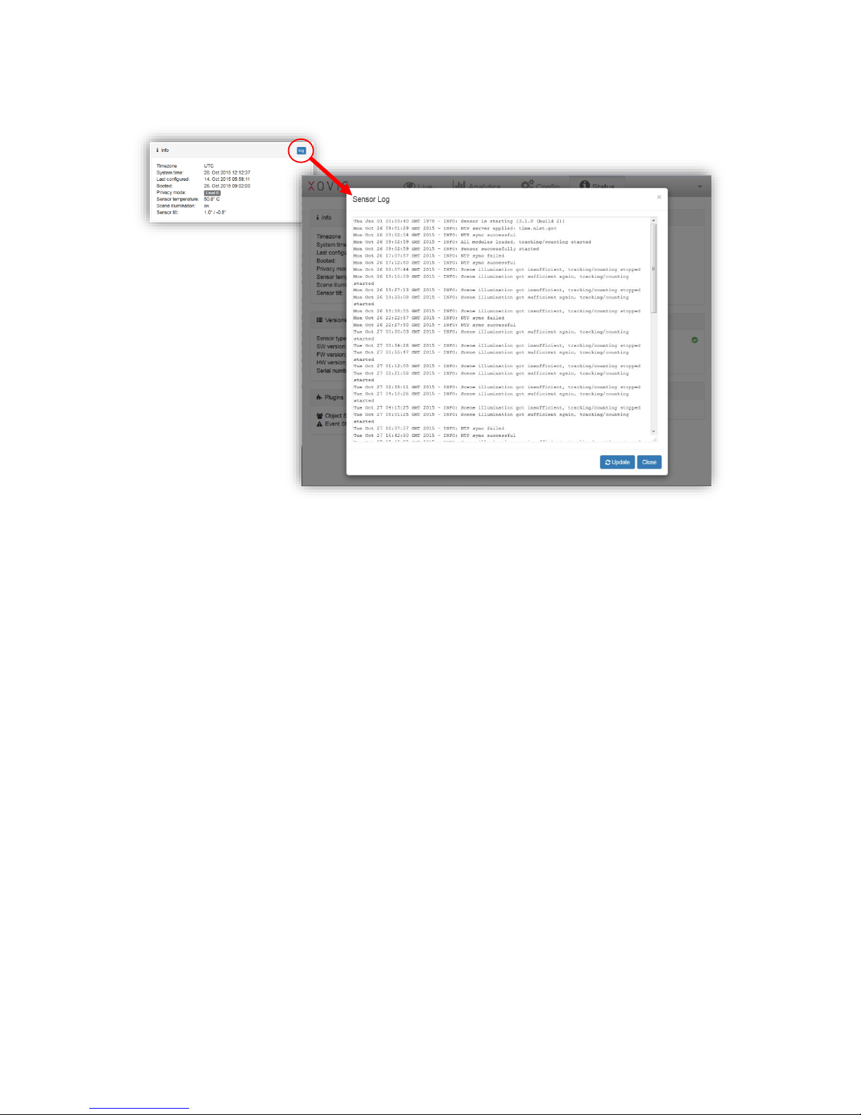
83 / 99 www.xovis.com
The “log”-button on the upper right corner of the Info box opens the detailed log view:
The log holds details about:
- Boot process
- NTP connectivity
- Push agent connectivity
- Scene illumination
- Configuration change
- Sensor reset
- Software upgrade
The log file size is limited to 200 KB. When reaching this limit, the log is automatically
rotated, i.e. the oldest entries are removed when new ones are added.
3.2.11.2 Data retention
The “Data retention” box informs about the amount of days that are stored on the sensor.
The sensor can store up to 122 full days for count lines and up to 61 full days for count zones.
This number of days is shared between the configured count items of each type (lines,
zones). For example, when using just one count line, the count values of this line will be
stored for 122 days. When using 2 count lines, both line values are stored for 61 days and so
on.
The date stated after “since” represents the oldest data available on the sensor for this count
item.
3.2.11.3 Version
The “Version” box holds a series of version information of the sensor:
Page 84
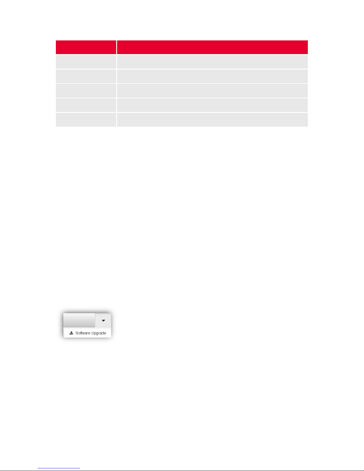
84 / 99 www.xovis.com
Item
Description
Sensor type
The device type, e.g. PC2
SW version
The version of the software currently running on the sensor
FW version
The firmware version
HW version
The hardware version
Serial number
Serial number/Ethernet MAC of the sensor
3.2.11.4 Connectivity
The “Connectivity” box shows the state of outgoing connections (NTP server, all configured
data push agents and the remote management server, if set). For every connection the
number of successful and failed tries is shown. The icon on the right of each connection
indicates, if the latest try succeeded or not (green check if succeeded, red alert if not).
3.2.11.5 Plugins
In the “Plugins” box, all plugins currently activated on the sensor are listed. The license state
as well as the running state (enabled / disabled) are shown.
3.2.11.6 Multisensor
The “Multisensor” box shows the status of the multisensor and the status of each single
sensor with its IP address connected in the multisensor array.
3.2.12 Firmware upgrade
The sensor allows to easily upgrade its software / firmware. The installation of firmware
upgrades can be done by clicking on the “Software Upgrade” menu entry in the context menu
(see chapter 3.2.6):
The following dialog appears:
Page 85
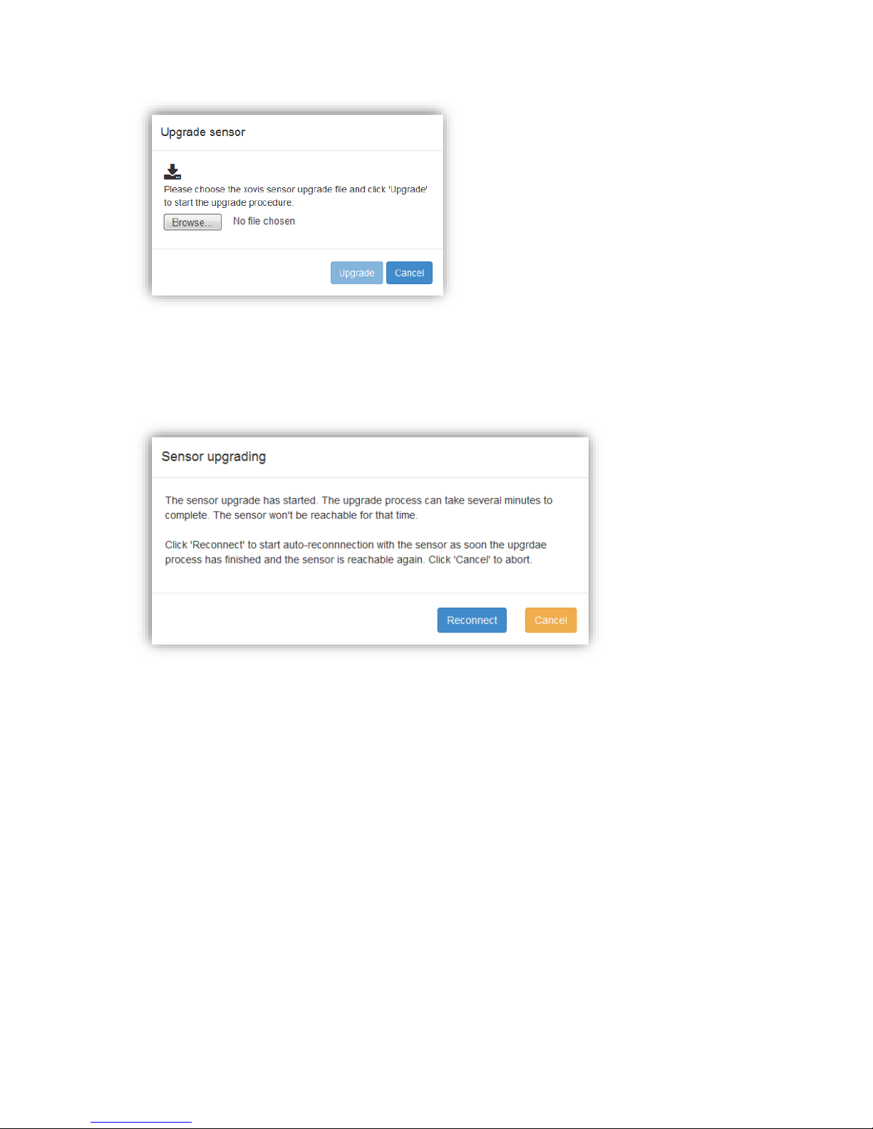
85 / 99 www.xovis.com
By clicking on the “Browse…” button, the firmware upgrade file can be chosen on the local
file system. The only supported file extension is .xfw. When a valid file is chosen, the
“Upgrade” button will get enabled. Clicking on it will start the upgrade / installation
procedure. The following dialog will be displayed:
By clicking “Reconnect”, the web GUI will automatically poll the sensor to observe when it is
back online and then automatically reconnect the web GUI.
Page 86
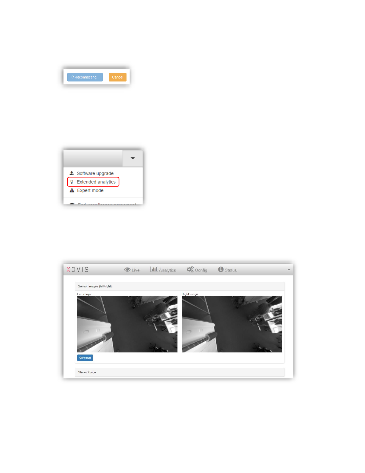
86 / 99 www.xovis.com
While waiting for the sensor to be online again, the “Reconnect” button will indicate the
reconnection with a rotating spinner icon as shown in Figure 51:
Figure 51: Reconnecting to the web GUI while upgrading
3.2.13 Extended analytics
The extended analytics offers two additional views helping in case of trouble shooting.
“Sensor images (left/right)” shows the grayscale image of both lenses. This can help to
identify dirt and scratches on the lenses. Furthermore, it also helps identifying obstacles
hanging from the ceiling which demand for a mask. Clicking on “Reload” gathers new
images.
The “Stereo image” box shows the actually processed depths image of the sensor. This can
help to verify the scene-calibration: If the floor is not colored blueish or shows a slope in
coloring, this indicates a false calibration.
Page 87
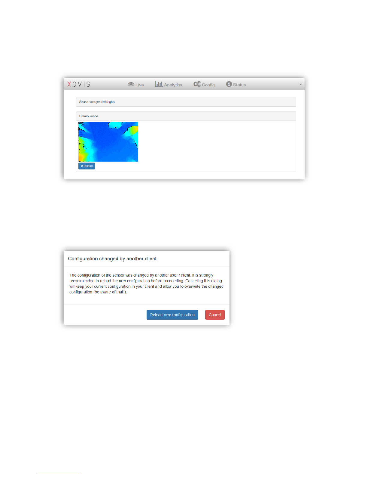
87 / 99 www.xovis.com
It is then recommended to perform a recalibration of the sensor (either re-start the setup
wizard or use the “shortcut” by clicking on the “mounting height” in the “Settings” part of the
“Config” view).
3.2.14 Configuration changes from another client
Whenever the sensors configuration gets changed by another client, i.e. when more than one
user is working on the sensor configuration at the same time, the web GUI will inform the
user about changes made by another client with the following dialog:
It is recommended to reload the new configuration to be up to date with the latest sensor
configuration. This can be done by just clicking on “Reload new configuration” in the dialog.
Page 88
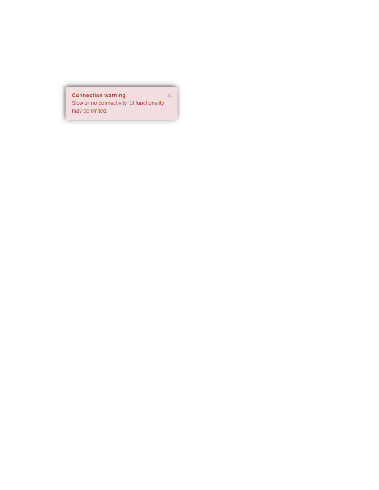
88 / 99 www.xovis.com
3.2.15 Connection warning
Whenever the network connection between the client and the sensor gets slow or broken,
the web GUI will inform the user with the following popup, appearing on the bottom right:
Figure 52: Connection warning
A connection break can be caused by multiple reasons, e.g. by a rebooting sensor, a running
firmware upgrade or just a communication issue in the local network (e.g. very low
bandwidth).
Whenever this message appears, working with the UI could get limited. With low connectivity,
image stream and count value updates can get delayed, for example. When the connection is
completely broken, the UI will not be updated at all. However, switching between the tabs
(Live, Statistics, Config, Status) and changes to the configuration can still be made. However,
saving the configuration changes will not succeed until the connection is established again.
Page 89
89 / 99 www.xovis.com
4 Troubleshooting
False behavior
Under some special conditions, the sensor can show an unwanted behavior. Examples for
such behavior are wrongly detected/generated persons or bubbles of a tracked person which
jumps to an object, e.g. a pillar.
Such issues occur rarely and are caused by a scene situation which disturbs the sensors
algorithm and leads to a false detection. Even if it is unlikely that such false behavior would
influence the counting accuracy of a sensor, it can be desirable to reduce such issues.
Masks
Depending on the actual disturbance, two types of masks can be used: Exclusion and taboo
masks.
As the sensor is robust against disturbances in most situations, masks will only be
necessary in few situations. Proactively drawing masks is therefore not required.
4.2.1 Exclusion masks
Exclusion masks define a zone as invalid for tracking. Same as with the floor mask, the
exclusion mask is oriented on the floor. As soon a person enters an exclusion mask, it will be
deleted immediately. A new person which is located in an exclusion mask won’t be generated
until it leaves the mask. The location thereby is always referenced to a persons’ foot position.
The exclusion mask can help to hinder false detections or bubbles sticking on objects like
pillars, walls or lamps. To identify situations where this mask could be used, it is
recommended to switch the sensor to foot coordinates. That way bubbles are projected to
the floor and potential problematic objects/regions can be identified easily. Refer to chapters
3.2.7.9.1 and 3.2.10.4 to learn how to change the coordinate mode.
A mirroring wall (metal or glass wall) is a common example where exclusion masks can be
used. When a sensor shows problems with bubbles occurring or jumping to the region on the
mirroring wall, the whole wall can simply be covered by an exclusion mask.
Another example for using an exclusion mask could be an information column in the
peoples’ pass way. Especially when located close to the border, the bubbles of persons
leaving the scene could jump to the column and stick there for a short period. To hinder this,
a simple exclusion mask covering the footprint of this column can be drawn.
Figure 53 shows an example for both of these situations. The left image (a) shows a scene
with a big mirroring wall on the left and an information column on the right bottom. The right
image (b) shows the same scene with exclusion masks applied.
Page 90
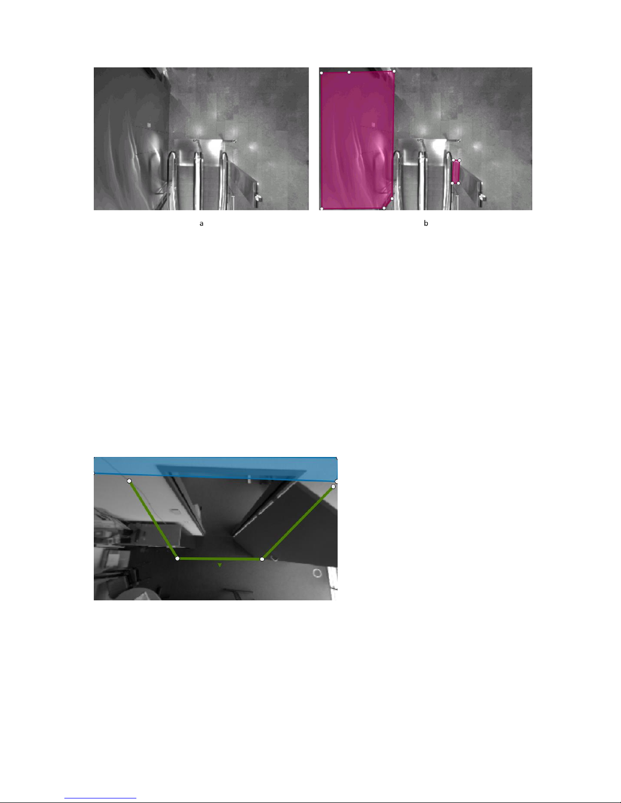
90 / 99 www.xovis.com
Figure 53: Exclusion mask on mirroring wall and information column
The drawing procedure is the same as with the floor mask (see chapter 3.2.7.6). Exclusion
masks are also added to the scene element list as soon as the initial drawing is finished.
4.2.2 Taboo masks
Taboo masks define areas completely excluded from the sensor’s processing. They can be
understood like black holes, i.e. areas where no image information at all is kept. In addition,
taboo masks act as artificial scene boundaries. The sensors algorithms benefit from the
information of such scene boundaries, e.g. for proper handling people leaving the scene.
Therefore scene boundaries which differ from the actual sensors view boundaries should be
marked by using taboo masks for everything behind that scene boundary.
Figure 54 shows an example situation where the doorway is masked by a taboo mask to
guarantee fast deletion of persons leaving through the door:
Figure 54: Taboo mask for marking the scene boundary
Furthermore taboo masks can be important to eliminate disturbing influence caused by
scene situations not processable by the sensors stereo vision algorithm. Such influences can
for example be caused by:
Signboards or monitors mounted within the sensors view
Unstructured or mirroring walls
Dark regions in strongly inhomogeneous illumination situations
Page 91
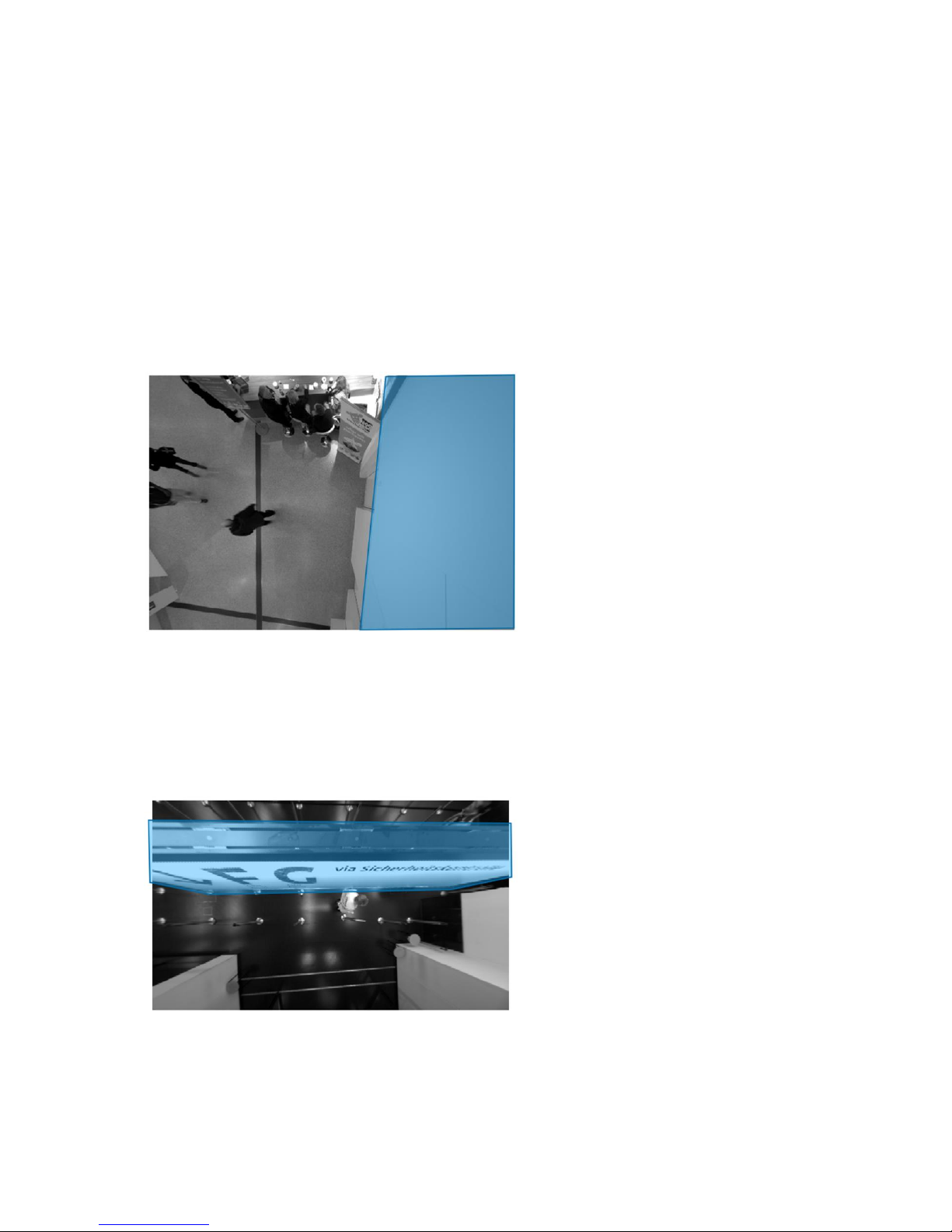
91 / 99 www.xovis.com
For better identifying objects influencing the internal processing, it is best to switch the
sensor to head coordinates. Refer to chapters 3.2.7.9.1 and 3.2.10.4 to learn how to change
the coordinate mode. Now, with coordinate mode set to “head”, false detections are shown
where they really appear.
Figure 55 shows a situation combining two reasons for using taboo masks in the same
scene: First, a significant part of the scene is covered by the wall which reaches towards the
sensor. This can cause disturbing artefacts which can influence the sensors vision
algorithms. Second, the situation shows two doors in the inner area of the scene, i.e. not at
the scene border, same as already in Figure 54. Telling the sensor about this artificial scene
boundary helps for proper person deletion when leaving through the doors. Masking out the
area appropriate eliminates such possible misbehavior:
Figure 55: Taboo mask on unstructured white wall and marking the scene boundary over two doors
Figure 56 shows a situation with a big sign located within the sensors view. As this sign is
very close to the sensor, the stereo vision processing could be disturbed. And, again as with
the situations in Figure 54 and Figure 55, it is important to tell the sensor about this scene
boundary. Otherwise person bubbles could stick at the sign when the person walks
underneath it. Masking out the sign appropriate eliminates such possible misbehavior.
Figure 56: Taboo mask on a sign within the sensor view
Note that, other than with floor masks, taboo masks usually cover slightly more than
necessary. This is important due to the fact, that disturbing artefacts which are masked out
by taboo masks show inexact dimensions and can slightly slop over their actual region.
Page 92
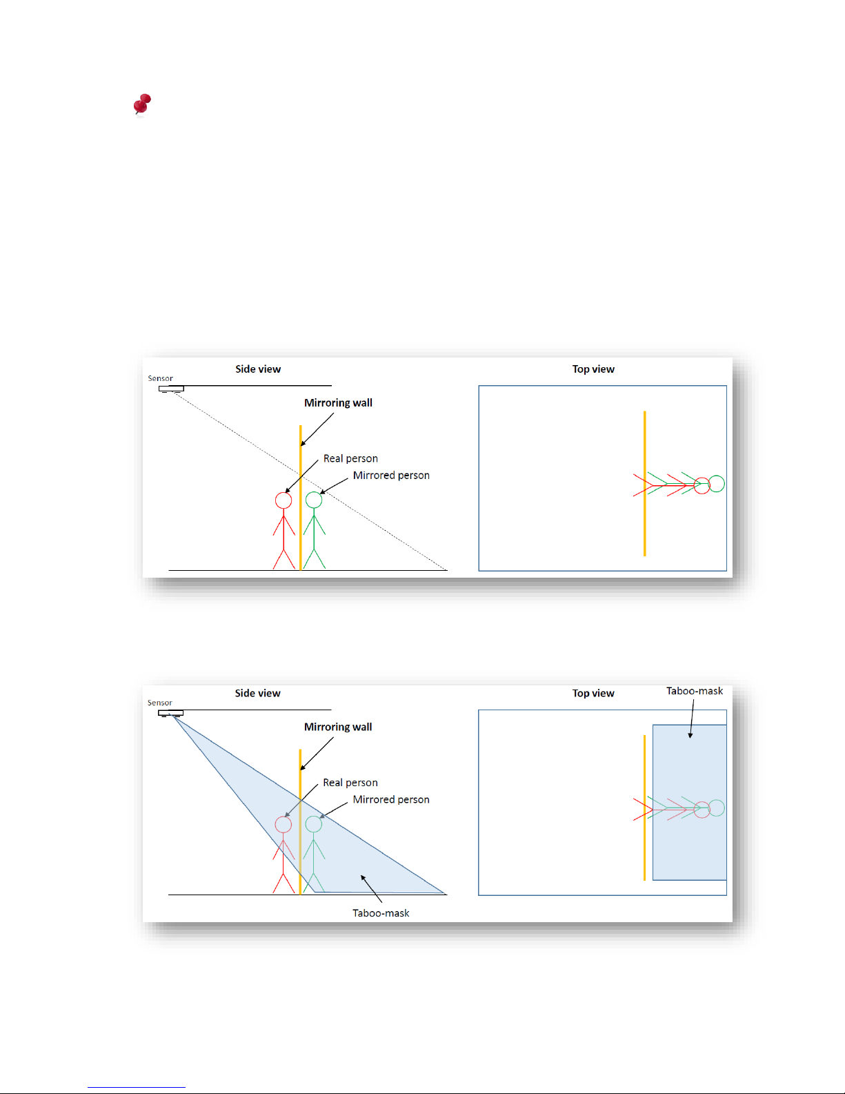
92 / 99 www.xovis.com
Taboo masks should cover slightly more than necessary to ensure robustness against a
slightly slopping over of disturbing artefacts.
The drawing procedure is the same as with the floor mask (see chapter 3.2.7.6). Taboo
masks are also added to the scene element list as soon as the initial drawing is finished.
4.2.3 Example for mask differentiation
The following example gives a better understanding on how the two masks work.
The following image illustrates a person walking close to a mirror (red) and the reflection of
the person (green).
As the green mirrored person shows valid criteria to the sensor for being a real person as
well, the sensor will track both of them. This is unwanted and can be addressed by using a
mask.
When using a blue mask, the complete area covered by this mask is cleared, i.e. shows no
information anymore. The sensor is blind in this area. This leads to the fact, that not only the
Page 93
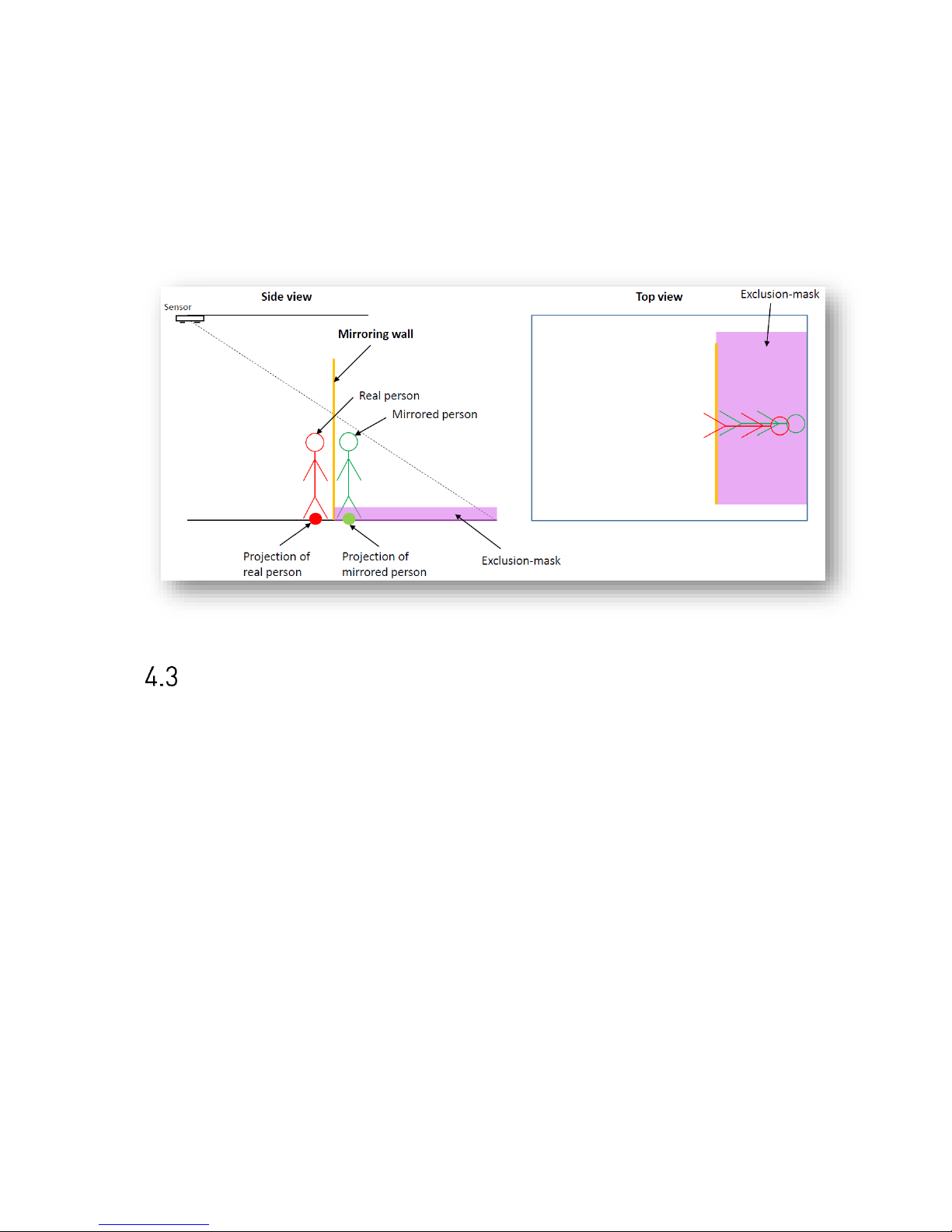
93 / 99 www.xovis.com
green (unwanted) person gets deleted but also big parts of the red one (it will be cut by the
blue mask). This will therefore also eliminate the track of the red person, which is unwanted.
Other with a purple mask. As the sensor scene is still completely processed, also in the area
covered by the purple mask, internally both persons will be tracked. But an additional check
will now lead to the deletion of the green person: As soon the foot position of a person is
located within the purple mask, it will get deleted immediately. For the sample situation, this
is exactly what the user was looking for.
Placement of dwell zones
The dwell time analysis uses a regular zone which is configured in the Config View. When
placing the zone, special care has to be taken that the dwell zone correctly lies within the
sensor’s tracking area.
The dwell time analysis only considers tracks which enter the zone across the zone’s border
and also leave the zone across the zone’s border. Tracks that are created or deleted within
the zone are not considered by the dwell time analysis.
The below image shows three tracks A, B and C:
Page 94
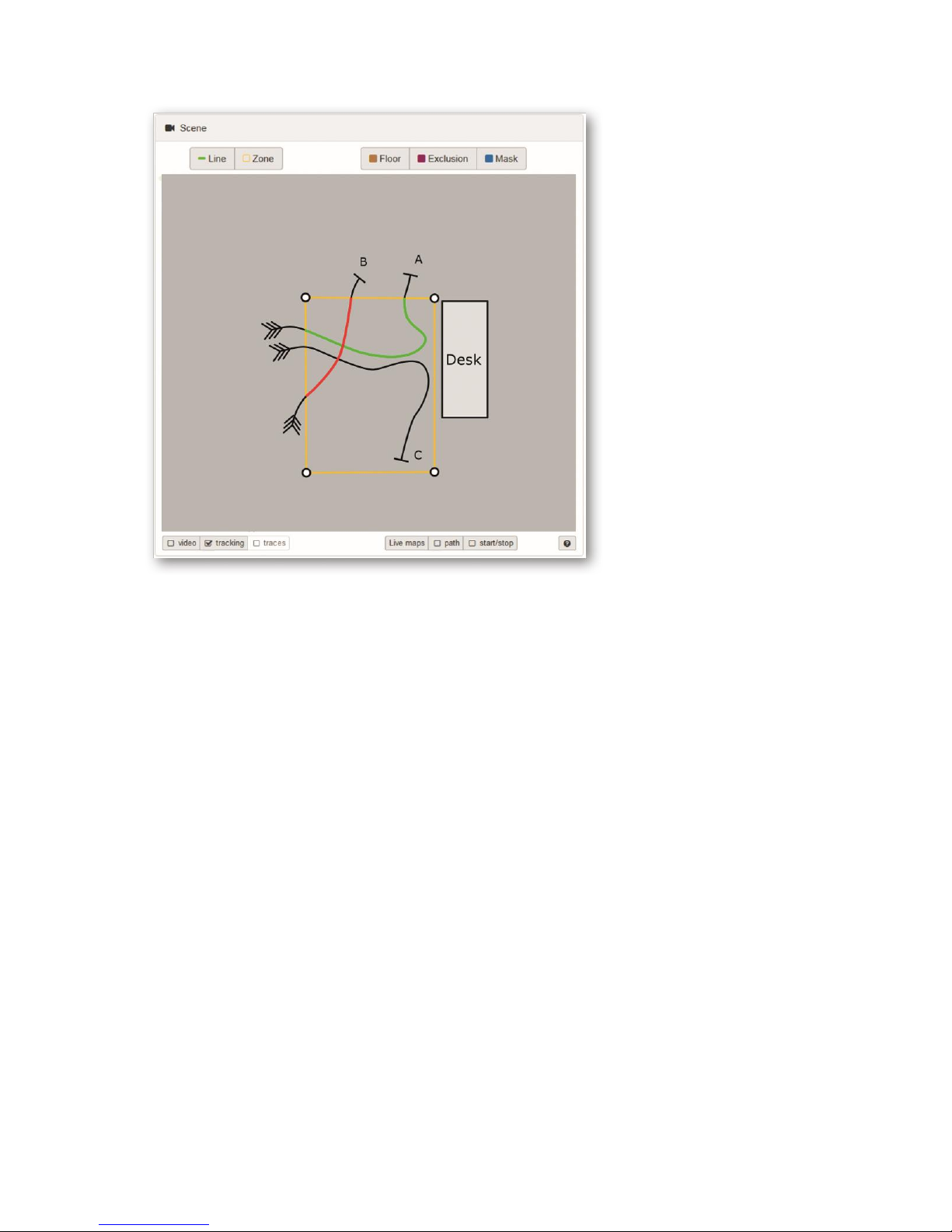
94 / 99 www.xovis.com
Figure 57: Illustration of different tracks and their influence on dwell time calculation
- Track A enters the dwell zone from the left, walks to the desk (where it is
waiting during the desk process) and then leaves the sensor’s tracking area
towards the top. The track is created AND deleted outside the dwell zone. Its
dwell time is calculated (time between the zone entry and the zone exit, green)
and is then used in the statistical dwell time analysis.
- Track B enters the dwell zone from the left, doesn’t go to the desk, but quickly
moves on and leaves towards the top. As its track is correctly created AND
deleted outside the dwell zone, the dwell time is calculated (time between the
zone entry and the zone exit, red). But as its dwell time was shorter than the
minimal dwell time its dwell time value will not be considered for further
statistical dwell time analysis.
- Track C enters the dwell zone from the left, walks to the desk and leaves the
sensor towards the bottom. Unfortunately, the sensor’s tracking area is not
large enough and the track is deleted before the track leaves the dwell zone.
The dwell time of this track is not calculated, because its deletion point is
inside the dwell zone.
The example of track C shows that special care has to be taken when placing the dwell zone
in order assure correct dwell time analysis, otherwise it could lead to a rather high amount
of not calculated dwell times
As shown in the figures below, the activation of start/stop points can be useful in order to
optimize the dwell zone placement.
Page 95
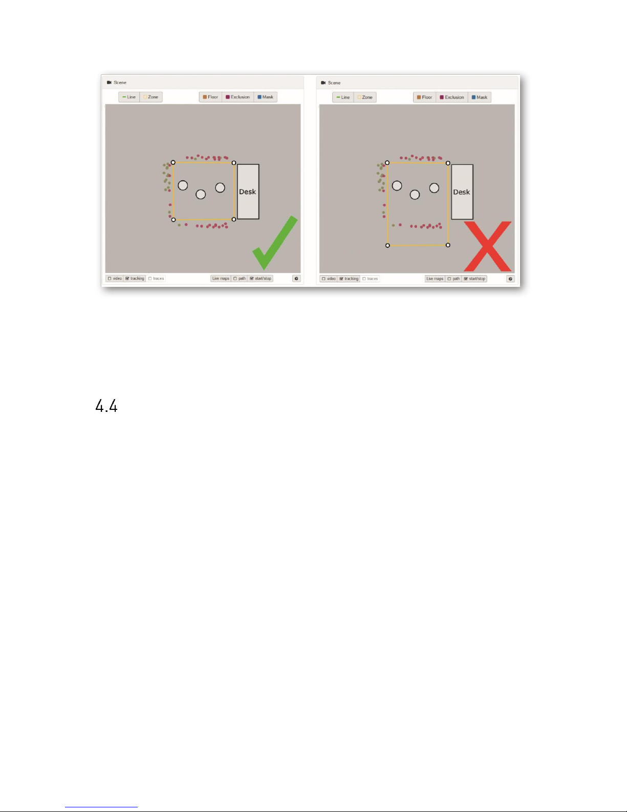
95 / 99 www.xovis.com
Figure 58: Start/stop points help identifying actual tracking area
The start/stop points (indicated as red and green points) show the limits of the sensor’s
tracking area. For optimal dwell time analysis, the dwell zone has to be placed inside the
sensor’s tracking area.
Time synchronization mechanism
The below flow diagram describes the time synchronization behavior depending on power or
internet connection loss.
Page 96
96 / 99 www.xovis.com
Prower Break Down
Internet connection OK
NTP-server set and reachable
Is this the first time you set-up
the sensor? Are you setting the
time manually now?
Yes
No
NTP time sync =>
time is valid
Quite valid time,
synchronization
recommended
Yes
No
Was the power break
only short, e.g. a
power cut only?
No
Invalid time,
synchronization
required
Yes
Sensor uses manually set time
Sensor uses last known time
before rebooting
and adds the
expected time of
the rebooting process => time is quite accurate
Sensor uses last known time before rebooting and adds the
expected time of
the rebooting process => due to long power
shutdown, time now is in the past
Page 97

97 / 99 www.xovis.com
5 Technical data
General
Temperature 0 – 45 °C
-25 – 60 °C (only PC2 with outdoor housing PA-PC2-OH)
Humidity 20 - 80 %
Size PC2: 130 mm x 94 mm x 30 mm (LxWxH)
PC3: 34.5 mm x 6.7 mm x 3.7 mm (LxWxH)
Weight PC2: 350 g (with plastic cover)
PC3: 750 g
Power max. 5 W
Connection RJ-45 Ethernet, Power over Ethernet (IEEE 802.3af), Class 0
Mounting height PC2: 2.2 – 6.0 m
PC3: 6.0 – 20.0 m
Data bandwidth Ideal bandwidth: >200 KB/s
sensor works best including the WebGUI (up to 4 frames per second
are delivered in the live view)
Recommended minimum for configuration: 100 KB/s
sensor works moderate with the WebGUI in use (live view provides limited
fps only)
Needed bandwidth for data transmission: <20 KB/s
sensor works, but without using the WebGUI (ok for operational use after
configuration). Actual needed bandwidth depends on how many DataPush
Agents, Object Streams etc. are in use.
Analytics
8 Multipoint count lines for counting in forward and backward direction
8 Multipoint count zones for measuring number of persons within the zone (occupancy)
“In/out” and “Late” count mode
Activation zones
Data retention of 122 days in total, divided by the amount of count lines in use
Plugin architecture
The sensors functionality can be extended by various plugins which run directly on the
sensor. Xovis offers a list of all available plugins.
Page 98

98 / 99 www.xovis.com
6 Certificates / Tests
Emission – Requirements
IEC/CISPR 22: 2005 +A1:2005; EN 55022:2006 A1:2007
Information technology equipment - Radio disturbance characteristics - Limits and methods of
measurement
Immunity – Requirements
IEC/CISPR 24: 1997 +A1:2001 + A2:2002; EN 55024:1998 A1:2001 +A2:2003
Information technology equipment - Immunity characteristics - Limits and methods of
measurements
Safety – Requirements
IEC 60950-1: 2005 (Second Edition) +Am 1: 2009 + Am 2: 2013
Safety of information technology equipment
FCC
Note: This equipment has been tested and found to comply with the limits for a Class B
digital device, pursuant to part 15 of the FCC Rules. These limits are designed to provide
reasonable protection against harmful interference in a residential installation. This
equipment generates, uses and can radiate radio frequency energy and, if not installed and
used in accordance with the instructions, may cause harmful interference to radio
communications. However, there is no guarantee that interference will not occur in a
particular installation.
If this equipment does cause harmful interference to radio or television reception, which can
be determined by turning the equipment off and on, the user is encouraged to try to correct
the interference by one or more of the following measures:
- Reorient or relocate the receiving antenna.
- Increase the separation between the equipment and receiver.
- Connect the equipment into an outlet on a circuit different from that to which the
receiver is connected.
- Consult the dealer or an experienced radio/TV technician for help.
Page 99

99 / 99 www.xovis.com
7 Custom Integration
API
Xovis offers the possibility to access raw sensor data directly by a platform independent API
and thereby provides an easy way to integrate Xovis sensors into third-party applications.
Detailed information on the sensor interface and custom integration can be found in the API
documentation. Interested integrators can contact Xovis to receive a copy of the API
documentation.
Plugin Architecture
The plugin architecture provided by the PC2 sensor can also be used for custom plugins.
Xovis offers service and guidelines for developing custom plugins which can be run directly
on the sensor. Interested integrators can contact Xovis for more information.
 Loading...